Embed Size (px)
Citation preview
1 / 11
Quantum correlations and entanglement infar-from-equilibrium spin systems
Mauritz van den Worm
National Institute of Theoretical Physics
Stellenbosch University
NITheP Bursars Workshop

| Introductory words 2 / 11
| Introductory words 2 / 11
| Introductory words 2 / 11
| Introductory words 2 / 11

| Introductory words 2 / 11
| Introductory words 2 / 11
| Introductory words 2 / 11
| Introductory words 2 / 11
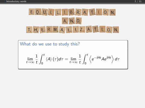
What do we use to study this?
limt→∞
1
t
∫ t
0〈A〉 (τ)dτ = lim
t→∞
1
t
∫ t
0
⟨e−iHtAe iHt
⟩dτ
| Introductory words 2 / 11
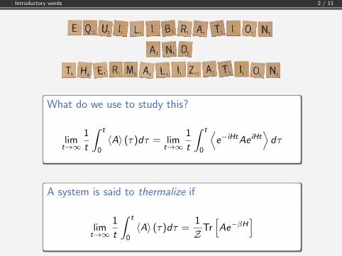
What do we use to study this?
limt→∞
1
t
∫ t
0〈A〉 (τ)dτ = lim
t→∞
1
t
∫ t
0
⟨e−iHtAe iHt
⟩dτ
A system is said to thermalize if
limt→∞
1
t
∫ t
0〈A〉 (τ)dτ =
1
ZTr[Ae−βH
]
| Introductory words 2 / 11
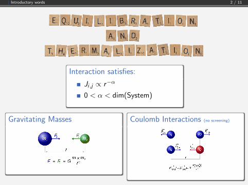
Interaction satisfies:
Ji ,j ∝ r−α
0 < α < dim(System)
Gravitating Masses Coulomb Interactions (no screening)
| Exact analytic results 3 / 11
| Exact analytic results 4 / 11
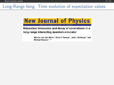
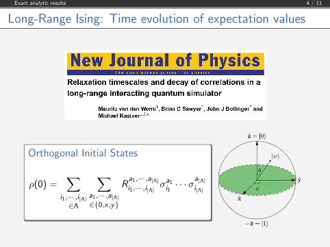
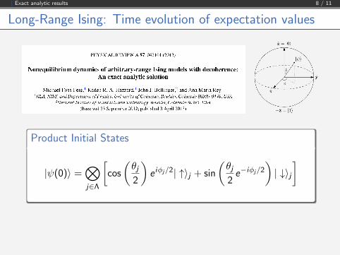
Long-Range Ising: Time evolution of expectation values

| Exact analytic results 4 / 11
Long-Range Ising: Time evolution of expectation values
Ingredients
D dimensional lattice Λ
H =⊗
j∈Λ C2j
Ji ,j = |i − j |−α
Long-range Ising Hamiltonian
H = −∑
(i ,j)∈Λ×Λ
Ji ,jσzi σ
zj − B
∑i∈Λ
σzi
| Exact analytic results 4 / 11
Long-Range Ising: Time evolution of expectation values
Orthogonal Initial States
ρ(0) =∑
i1,··· ,i|Λ|∈Λ
∑a1,··· ,a|Λ|∈{0,x ,y}
Ra1,··· ,a|Λ|i1,··· ,i|Λ| σ
a1i1· · ·σa|Λ|i|Λ|

| Exact analytic results 4 / 11
Long-Range Ising: Time evolution of expectation valuesGraphical Representation of Correlation Functions
XΣ0x\HtL
XΣ-1x Σ1
x\HtLXΣ-1
yΣ1
y\HtLXΣ-1
yΣ1
z \HtL
Α = 0.4
0.01 0.1 1 10t
0.2
0.4
0.6
0.8
1.0
XΣiaΣ j
b\HtL
Figure : Time evolution of the normalized spin-spin correlators. The respectivegraphs were calculated for N = 102, 103 and 104. Notice the presence of thepre-thermalization plateaus of the two spin correlators.

| Exact analytic results 5 / 11
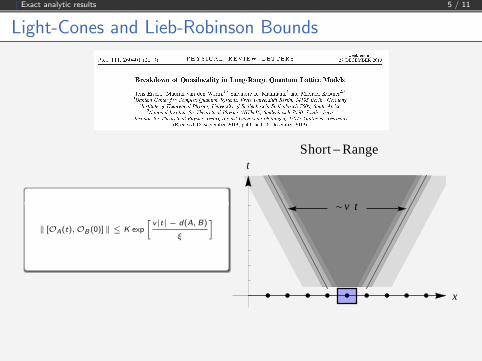
Light-Cones and Lieb-Robinson Bounds
| Exact analytic results 5 / 11
Light-Cones and Lieb-Robinson Bounds
‖ [OA(t),OB (0)] ‖ ≤ K exp
[v|t| − d(A, B)
ξ
] ~v t
x
t
Short-Range
| Exact analytic results 5 / 11
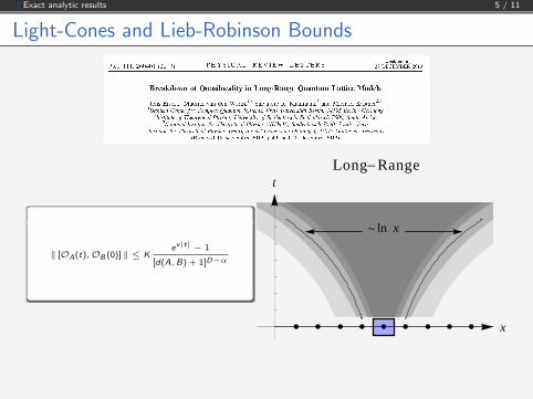
Light-Cones and Lieb-Robinson Bounds
‖ [OA(t),OB (0)] ‖ ≤ Kev|t| − 1
[d(A, B) + 1]D−α
~ ln x
x
t
Long-Range
| Exact analytic results 5 / 11
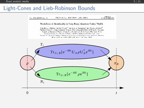
Light-Cones and Lieb-Robinson Bounds
Ρ Π B
TrL� B @e- iHt UA ΡUA†
e iHt D
TrL� B @e- itH ΡeiHt D
0 t
Tt
N t
| Exact analytic results 5 / 11
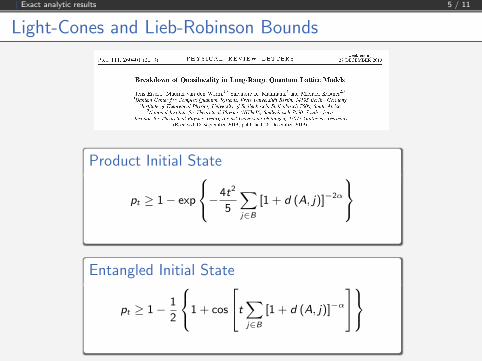
Light-Cones and Lieb-Robinson Bounds
Product Initial State
pt ≥ 1− exp
−4t2
5
∑j∈B
[1 + d (A, j)]−2α
Entangled Initial State
pt ≥ 1− 1
2
1 + cos
t∑j∈B
[1 + d (A, j)]−α
| Exact analytic results 5 / 11
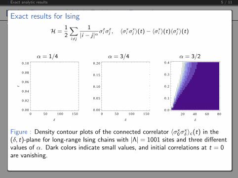
Light-Cones and Lieb-Robinson BoundsExact results for Ising
H =1
2
∑i 6=j
1
|i − j |α σzi σ
zj , 〈σx
i σxj 〉(t)− 〈σx
i 〉(t)〈σxj 〉(t)
α = 1/4 α = 3/4 α = 3/2
0 50 100 150
0.00
0.02
0.04
0.06
0.08
0.10
∆
t
0 50 100 150
0.00
0.05
0.10
0.15
0.20
∆
20 40 60 80
0.0
0.1
0.2
0.3
0.4
∆
Figure : Density contour plots of the connected correlator 〈σx0σ
xδ 〉c(t) in the
(δ, t)-plane for long-range Ising chains with |Λ| = 1001 sites and three differentvalues of α. Dark colors indicate small values, and initial correlations at t = 0are vanishing.
| Exact analytic results 5 / 11
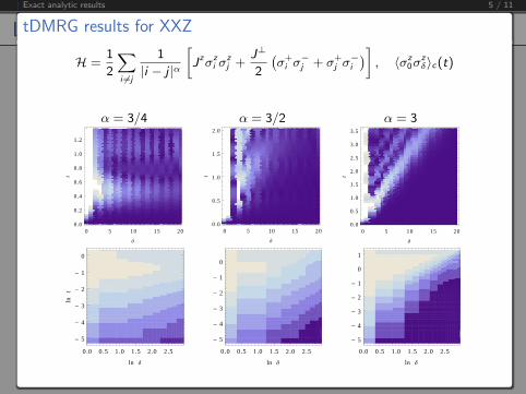
Light-Cones and Lieb-Robinson BoundstDMRG results for XXZ
H =1
2
∑i 6=j
1
|i − j |α
[Jzσz
i σzj +
J⊥
2
(σ+i σ−j + σ+
j σ−i
)], 〈σz
0σzδ〉c(t)
α = 3/4 α = 3/2 α = 3
0 5 10 15 20
0.0
0.2
0.4
0.6
0.8
1.0
1.2
∆
t
0 5 10 15 20
0.0
0.5
1.0
1.5
2.0
∆
t
0 5 10 15 20
0.0
0.5
1.0
1.5
2.0
2.5
3.0
3.5
∆
t
0.0 0.5 1.0 1.5 2.0 2.5
- 5
- 4
- 3
- 2
- 1
0
ln ∆
lnt
0.0 0.5 1.0 1.5 2.0 2.5
- 5
- 4
- 3
- 2
- 1
0
ln ∆
0.0 0.5 1.0 1.5 2.0 2.5
- 5
- 4
- 3
- 2
- 1
0
1
ln ∆
| What is being done experimentally? 6 / 11

| What is being done experimentally? 6 / 11
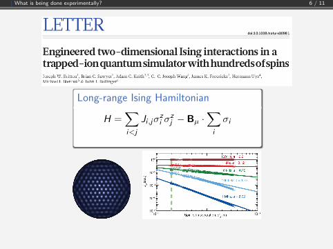
Current state of the art
H =1
2
∑i 6=j
[JxijS
xi S
xj + Jy
ij Syj S
yi + Jz
ijSzi S
zj
][To appear in PRA, Arxiv:1406.0937 - Kaden Hazzard, MVDW, Michael Foss-Feig, et al.]
| What is being done experimentally? 6 / 11
Long-range Ising Hamiltonian
H =∑i<j
Ji ,jσzi σ
zj − Bµ ·
∑i
σi
| What is being done experimentally? 6 / 11
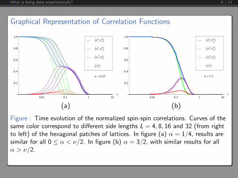
Graphical Representation of Correlation Functions
YΣix]
YΣiy
Σ jz]
YΣiy
Σ jy]
YΣix
Σ jx]
Α = 0.25
0.01 0.1 1 10t
0.2
0.4
0.6
0.8
1.0
YΣix]
YΣiy
Σ jz]
YΣiy
Σ jy]
YΣix
Σ jx]
Α = 1.5
0.01 0.1 1 10t
0.2
0.4
0.6
0.8
1.0
(a) (b)
Figure : Time evolution of the normalized spin-spin correlations. Curves of thesame color correspond to different side lengths L = 4, 8, 16 and 32 (from rightto left) of the hexagonal patches of lattices. In figure (a) α = 1/4, results aresimilar for all 0 ≤ α < ν/2. In figure (b) α = 3/2, with similar results for allα > ν/2.

| What is being done experimentally? 6 / 11
Ising XXZ
| Exact analytic results 7 / 11
| Exact analytic results 8 / 11
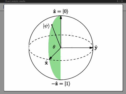
Long-Range Ising: Time evolution of expectation values
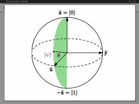
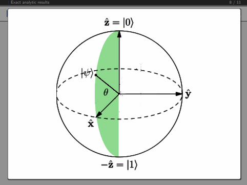
Product Initial States
|ψ(0)〉 =⊗j∈Λ
[cos
(θj2
)e iφj/2| ↑〉j + sin
(θj2e−iφj/2
)| ↓〉j
]

| Exact analytic results 8 / 11
Long-Range Ising: Time evolution of expectation values
Product Initial States
|ψ(0)〉 =⊗j∈Λ
[cos
(θj2
)e iφj/2| ↑〉j + sin
(θj2e−iφj/2
)| ↓〉j
]
| Exact analytic results 8 / 11
Long-Range Ising: Time evolution of expectation values
Product Initial States
|ψ(0)〉 =⊗j∈Λ
[cos
(θj2
)e iφj/2| ↑〉j + sin
(θj2e−iφj/2
)| ↓〉j
]
| Exact analytic results 8 / 11
Long-Range Ising: Time evolution of expectation values
Product Initial States
|ψ(0)〉 =⊗j∈Λ
[cos
(θj2
)e iφj/2| ↑〉j + sin
(θj2e−iφj/2
)| ↓〉j
]
| Exact analytic results 8 / 11
Long-Range Ising: Time evolution of expectation values
Product Initial States
|ψ(0)〉 =⊗j∈Λ
[cos
(θj2
)e iφj/2| ↑〉j + sin
(θj2e−iφj/2
)| ↓〉j
]
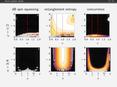
| Exact analytic results 9 / 11
dB spin squeezing entanglement entropy concurrenceϕ
=π/2
a
0.0 0.5 1.0 1.5 2.00
2
4
6
8
Α
t
b
0.0 0.5 1.0 1.5 2.00
2
4
6
8
Α
t
c
0.0 0.5 1.0 1.5 2.00
2
4
6
8
Α
t
α=
3/4
d
0Π
4
Π
2
3 Π
4Π
0
2
4
6
8
j
t
e
0Π
4
Π
2
3 Π
4Π
0
2
4
6
8
j
tf
0Π
4
Π
2
3 Π
4Π
0
2
4
6
8
jt
| Take home message 10 / 11
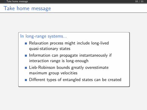
Take home message
In long-range systems...
Relaxation process might include long-livedquasi-stationary states
Information can propagate instantaneously ifinteraction range is long-enough
Lieb-Robinson bounds greatly overestimatemaximum group velocities
Different types of entangled states can be created
| Collaborators 11 / 11
Collaborators
Michael KastnerSupervisor
John BollingerNIST
Boulder, Colorado
Brian SawyerNIST
Boulder, Colorado
Emanuele Dalla TorreBar Ilan UniversityTel Aviv, Isreal
Tilman PfauUniversitat StuttgartStuttgart, Germany
Ana Maria ReyJILA
Boulder, Colorado
Kaden HazzardJILA
Boulder, Colorado
Michael Foss-FeigJQI
Gaithersburg, Maryland
Salvatorre ManmanaUniversity of GottingenGottingen, Germanay
Jens EisertFreie UniversitatBerlin, Germany