A

summer internship report

on

Instrumentation for dayglow photometry

Submitted by:

Praveen Kumar Singh Department of Environmental Science

Central University of Rajasthan

Under guidance of:

Prof. Duggirala Pallamraju Space and Atmospheric Science Division (SPA-SC),

Physical Research Laboratory

Physical Research Laboratory Navrangpura, Ahmedabad-380009

Certificate

This is to certify that the report entitled “Instrumentation for dayglow

photometry” is a bonafied work carried out by Mr. Praveen Kumar Singh under

the guidance and supervision of Prof. Duggirala Pallamraju at Physical Research

Laboratory, Ahmedabad.

To the best of my knowledge and belief, this work embodies the work of candidate

himself, has duly been completed and fulfills the requirement of the summer

internship Program (SIP-2015).

Prof. Duggirala Pallamraju

Space and Atmospheric Science Division (SPA-SC),

Physical Research laboratory,

Ahmedabad

i

Acknowledgement

I acquire this opportunity with much pleasure to acknowledge the invaluable

assistance of Physical Research Laboratory and all the people who have helped me

through the course of my journey in successful completion of this summer

internship.

I wish to express my sincere gratitude to my Guide, Prof. Duggirala Pallamraju,

Professor, Space and Atmospheric Science Division for his guidance, help and

motivation. Apart from the subject of my study, I learnt a lot from him, which I

am sure, will be useful in different stages of my life. I would like to thank Mr.

Kedar A. Phadke, Scientist-SC for his help in understanding methodology as well

as various instruments I came across.

I would like to thank Dr. Bhushit G. Vaishnav, Head, Academic Services for

providing me with this wonderful opportunity to work at Physical Research

Laboratory. I express my thanks to Mr. Deepak Kumar Karan, Senior Research

Fellow for his kind cooperation during the period of my summer internship. I also

express my thanks to Dirgha and Sharanya, who shared work space with me.

I am grateful to my friends who gave me a pleasant environment to work for entire

duration of my internship. Last but not the least I would like to express my special

thanks to my family for their continuous motivation and support.

Regards,

Praveen Kumar Singh

Dated:

ii

Index

No. Contents Page no.

Certificate i

Acknowledgement ii

1 Airglow 1

2 Significance of airglow measurements 3

3 Challenges of dayglow measurements 4

4 PMT based dayglow photometer 7

5 CCD based dayglow photometer 8

6 Production Mechanisms of Dayglow 12

7 Summary 14

8 Bibliography 15

1

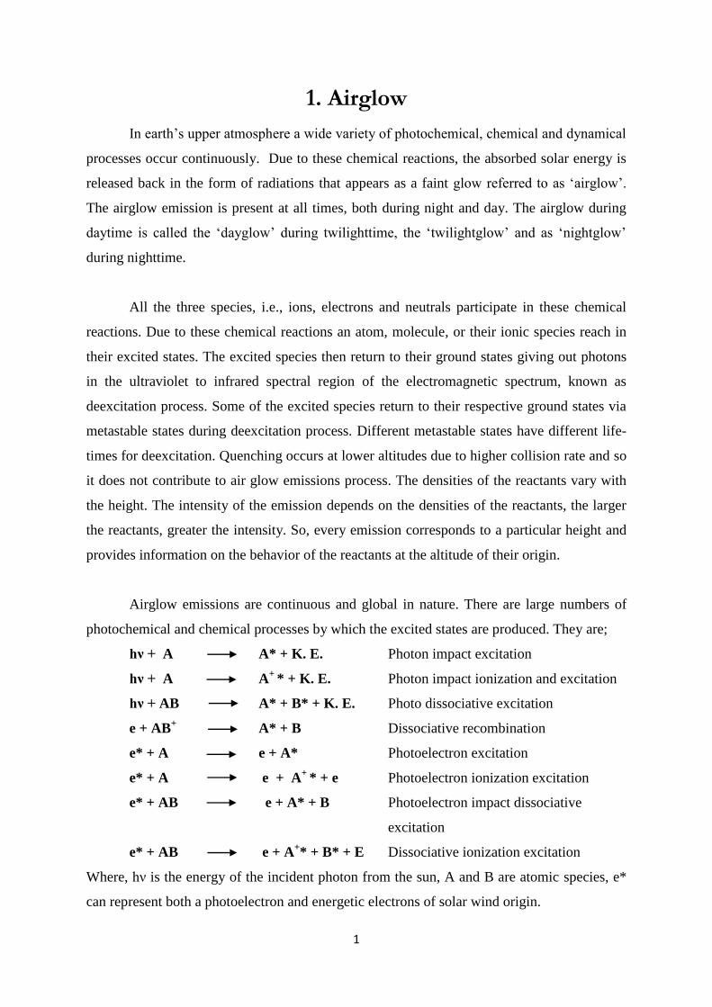
1. Airglow

In earth’s upper atmosphere a wide variety of photochemical, chemical and dynamical

processes occur continuously. Due to these chemical reactions, the absorbed solar energy is

released back in the form of radiations that appears as a faint glow referred to as ‘airglow’.

The airglow emission is present at all times, both during night and day. The airglow during

daytime is called the ‘dayglow’ during twilighttime, the ‘twilightglow’ and as ‘nightglow’

during nighttime.

All the three species, i.e., ions, electrons and neutrals participate in these chemical

reactions. Due to these chemical reactions an atom, molecule, or their ionic species reach in

their excited states. The excited species then return to their ground states giving out photons

in the ultraviolet to infrared spectral region of the electromagnetic spectrum, known as

deexcitation process. Some of the excited species return to their respective ground states via

metastable states during deexcitation process. Different metastable states have different life-

times for deexcitation. Quenching occurs at lower altitudes due to higher collision rate and so

it does not contribute to air glow emissions process. The densities of the reactants vary with

the height. The intensity of the emission depends on the densities of the reactants, the larger

the reactants, greater the intensity. So, every emission corresponds to a particular height and

provides information on the behavior of the reactants at the altitude of their origin.

Airglow emissions are continuous and global in nature. There are large numbers of

photochemical and chemical processes by which the excited states are produced. They are;

hν + A A* + K. E. Photon impact excitation

hν + A A+

* + K. E. Photon impact ionization and excitation

hν + AB A* + B* + K. E. Photo dissociative excitation

e + AB+ A* + B Dissociative recombination

e* + A e + A* Photoelectron excitation

e* + A e + A+

* + e Photoelectron ionization excitation

e* + AB e + A* + B Photoelectron impact dissociative

excitation

e* + AB e + A+* + B* + E Dissociative ionization excitation

Where, hν is the energy of the incident photon from the sun, A and B are atomic species, e*

can represent both a photoelectron and energetic electrons of solar wind origin.

2

The excitation processes can be categorized as; (a) the excitation by external agencies

such as solar photons and particle precipitation, and, (b) the mutual interaction amongst the

atmospheric species. The process (b) does not require external source and so it can be

operative at all the times i.e. day and night, where-as processes of the first category, those are

due to solar photons they are operative only during the daytime.

Airglow studies carried out at different time periods give information about the

dynamics present at that time and about their various parameters. There are a number of

experiments performed successfully to measure the twilightglow and nightglow.

Measurement of nightglow is easy because background continuum is absent. The dayglow

emission intensity is very low in comparison to the background solar continuum and

measurement is not easy as compared to nightglow.

Airglow emissions occur in wavelengths ranging from ultraviolet to infrared but we

are interested here in 630.0 nm emission line only, which is also known as oxygen red line

and it occurs in the thermosphere.

3

2. Significance of airglow measurements

In remote sensing technique we collect data from a distance without being in contact

with the object, when we illuminate the object by an artificial source then it is called active

remote sensing. When we collect photon of the object illuminated by natural source then it is

called passive remote sensing. Optical investigation of airglow is somewhat similar to passive

remote sensing of the upper atmosphere. Ground-based investigations by photometry and

spectrometry can provide us enough data to understand the behavior of the upper atmosphere

at different heights.

1. Airglow emission intensity has a direct relationship with the reacting species and

we can obtain information about the vertical distribution of species in ionosphere.

2. The optical techniques have their major importance in the study of neutral

dynamics of thermosphere because we cannot obtain data by using RADAR techniques.

3. Gravity waves influence the chemistry and composition of the thermosphere. The

airglow emission intensity also changes due to it. The spatial variation in emission intensity

reflects the characteristics of the gravity waves.

4. Various airglow emissions originate at different heights. By measuring the

intensities at different wavelengths nearly simultaneously one can infer the vertical

propagation of waves from one region to another thereby giving important clues on the mode

of coupling of these different regions.

In nighttime all the above mentioned studies have been carried out. Some of these

studies have also been centered at during twilighttime. However, very less number of studies

have been carried out in daytime.

Next section deals with the challenges of daytime measurement of emissions and

includes a brief note on experiments performed in past, around the globe.

4

3. Challenges of dayglow measurements

The presence of solar scattered background continuum which is of the order of Mega

Rayleighs of magnitude is much greater than the dayglow emission intensity which of the

order of Kilo Rayleighs makes the measurement of dayglow emissions very challenging.

Therefore, innovative and efficient methods have to be employed to extract the dayglow

emissions from strong solar continuum. There had been few attempts in the past to separate

out the weak emission features from the strong continuum background and with limited

success.

Blamont and Donahue (1964) tried to measure the sodium D lines by scanning the

line at 0.2-Å resolution and subtracting the normalized solar spectrum to remove the

Fraunhofer structure. The output was unexpectedly of high intensities of ~ 30 KR and it could

be contribution of direct solar radiation along with the scattered part of the solar radiation.

This technique was used for those limited dayglow lines, which can be resonantly scattered

by a vapor cell.

Bens et al. (1965) employed a combination of high and low resolution Fabry-Perots

(F-P) in series and an interference filter acted as monochromator at fixed wavelength and

obtained signatures of dayglow intensities. They performed a sequence of experiments with

varied instrumentation and made a comparison between the sky spectrum with the solar

spectrum. They just detected the emission lines and no conclusions were obtained.

Jarrett and Hoey (1963) employed a single low resolution F-P etalon and an

interference filter to obtain a fringe system at 630.0 nm on photographic plate. The observed

fringe system was questionable because Fraunhofer lines could also produce such images.

Noxon and Goody (1962) used the polarization property of the background to reduce

it. They employed a chopping mechanism at the entrance slit of an Ebert Scanning

spectrometer. The one half of the slit was covered with a polarizer and the other half with an

optical attenuator. The signals through the two halves of the slit were made equal for the

strongly polarized, scattered, sunlight at right angles to the sun so that the resulting

cancellation is independent of the intensity i.e. independent of the presence of Fraunhofer

lines. Dayglow emission lines which were unpolarized were efficiently modulated and

detected. The spectral scanning polarimeter was insensitive to the Fraunhofer lines but

random noise and real fluctuations in polarization associated with these lines were

responsible for the failure of this technique.

5

A photometer with a unique radial chopping mechanism was developed by Desai et al

(1979). They had used it for detection of rocket released lithium clouds during daytime. It

was constructed by using pressure tuned F-P, an interference filter of 7.5 Å bandwidth and a

mask that isolates two concentric zones of equal angular width. They had isolated two zones

of the same area, one containing the line of interest and the other just beyond this line, and

obtained the difference between these two which gave the contribution due to the signal

alone. The basic assumption is that the contribution due to the background at and

immediately away from the emission feature is identical.

Narayanan et al (1989) had developed a unique photometer for the measurement of

daytime OI 630.0 nm emission. The photometer employed a pressure tuned low resolution

(104) F-P etalon, temperature tuned narrowband (3 Å) interference filter, radial chopper and

up/down counting system. The radial chopper had two masks one is fixed and other is

rotating. The fixed disk passed through a optocouplar and enabled the generation of reference

pulses. Due to rotation of rotating mask the light passed through the system alternatively,

once through the central zone (signal plus background) and second time through the annular

zone (background). Reference pulse had acted as control pulse for the up/down counter and

difference between the number of pulses corresponding to the inner and outer zones

measured. The difference in counts had added up for defined time duration, passed onto a

digital to analog converter and plotted in X-T recorder. Total number of counts had recorded

in the other channel of X-T recorder simultaneously. The basic problem with the radial

chopping mechanism in this system was that the zones were never completely isolated and

there had always been a finite contribution from one zone when the measurements are made

through the other. Proper and complete subtraction of the background light is thus not

possible.

Figure 1. Schematic diagram of the dayglow photometer developed by

Narayanan et al (1989)

6

Rees et al (2000) developed an instrument and obtained a true image of daytime

aurora which consists an imaging optical spectrograph illuminated by a wide angle lens based

on two capacitance stabilized F-P etalon operated in series with each other and a narrow band

interference filter. The etalon plate gaps were 3.0 mm and 278 µm respectively. Interference

fringes formed by the etalons were imaged by a 300 mm lens onto a 1024×1024 pixel 16 bit

charge coupled device (CCD) chip. They captured two dimensional image of the sky in

which wavelength was a unique function of radius. They obtained image of 630.0 nm aurora

emission as a bright ring approximately 80% of the radial distance from the image center to

the edge. By varying the optical path differences of both etalons, a sequence of ten images, as

the 630.0 nm ring were captured at different radii and a complete two dimensional image of

sky at λ=630.0 nm was build. The procedure

followed in three steps; first, wavelength map was

generated for each individual sky image such that

each pixel represented the central wavelength of the

spectral distribution that illuminated the

corresponding pixel in the sky image. In second step,

the sky emission feature was extracted from each

image. The third analysis step was to construct the 2-

dimensional monochromatic image from ten different

image radii.

Figure 2. The sky image captured

by Rees et al (2000)

7

4. PMT based dayglow photometer

An instrument called dayglow photometer (DGP) was developed by Narayanan et al

(1989) to conduct daytime airglow studies. The photometer employed a pressure tuned low

resolution (104) F-P etalon, temperature tuned narrowband (3 Å) interference filter centered

(tuned) at 630.0 nm, a mask system, photo-multiplier tube (PMT) and data acquisition

system. The combination of two masks, a stator and a rotor made up the mask system. The

stator was divided into zones of 12 sections of equal areas, six segments are opaque and six

are transparent. The triangular and 'trapezoidal' segments are radially separated and hence

form the 'inner' and 'outer' annular zones. The rotor mask also had sections divided in a

similar way, except that there were only three transparent triangular segments, the diameter

of the same being equal to the outer dimensions of the outer zone (Pallamraju, 1996). This

mask had overcome the limitation encountered in the earlier version employed by Narayanan

et al. (1989). Another advantage was the area of light collection was more now; the flux

gathered is increased by a factor of 2 to 3 for the same intensity level. This mask system in

conjunction with the F P etalon, and synchronous photon counting systems made it possible

to remove the background contribution. Further, the signal plus background and the

background channels were now clearly separated in time due to the presence of the null zone.

This version of dayglow photometer yielded several exciting results of low and equatorial

electrodynamics.

8

5. CCD based dayglow photometer

In the present project multiple changes have been made in the old design of DGP. The

new instrument has many improvements over PMT based photometer. It uses CCD detector

instead of PMT. The use of CCD improved the resolution of the instrument significantly and

the chances of adverse effects due to the use of high voltage are now reduced to zero. The

instrument does not use any rotating parts because the mask system is removed. We are able

to capture two dimensional images which can be stored in the computers digitally and

processed by using digital techniques.

5.1. Technical details

This instrument makes use of a narrow bandwidth (3 Å) interference filter to isolate

the wavelength of interest and a F-P etalon of 500 µm air gap is used to produce a fringe

pattern and essentially work as a very high spectral resolution filter. The fringe pattern

obtained from F P etalon is imaged onto a CCD of 1391×1039 pixel size by using a lens of

100 mm focal length. The following section deals with the working of each of the above

mentioned components:

i. Interference filter:

The inference filter used in this instrument has a narrow bandwidth of 3 Å and

centered at the wavelength 630.0 nm.

ii. Fabry-Perot etalon:

The F-P used in this instrument has an air gap (optical thickness) of 500 µm and

reflectance of 0.85. The interference formula for this etalon can be written as,

where, n, λ, µ and t are the order of the wavelength interference, wavelength of the radiation,

refractive index of the medium between the etalon plates and optical thickness, respectively.

The spectral resolution of the etalon at any wavelength λ depends upon the distance between

the two optical plates i.e. optical thickness t.

If the medium between the plates is air, then µ = 1 and our operating wavelength λ = 630 nm,

the order of the wavelength n is given by,

9

n = 1587

Inter fringe distance better known as free spectral range of an etalon at that wavelength, is

given as,

For etalon used in this instrument the FSR turns out to 0.3969 nm or 0.4 nm (for λ = 630 nm).

Resolving power is given as the product of the order n (for wavelength λ) and finesse

F, of an F P. Hence,

Finesse F of an F-P depends upon the reflectivity of the plates, here r = 0.85

F = 19.31 for r = 0.85

Figure 3. Schematic diagram of CCD based DGP

10

Resolving power of a F-P is,

R = 0.31×105

If we examine the fringe pattern formed when a F-P etalon is illuminated by a

monochromatic light source, the maxima occurs when, satisfied, and

minima when

.

iii. The Charge Coupled Device (CCD):

A Sony ICX285AL CCD sensor used in this instrument. It is a diagonal 11 mm (Type

2/3) interline CCD solid-state image sensor with a square pixel array. The CCD is

monochrome and has pixel resolution of 1391×1039, nearly 1.45 Mega Pixels. The size of

each pixel is 6.45µm×6.45µm. The peak value of quantum efficiency is 65% at 540 nm and

sensitivity range is 300 nm – 1050 nm. The value of dark current is 0.0005 eˉ/pixel/sec at

0°C. Readout noise is 3.7 eˉ and gain is 0.267 eˉ/ADU. Minimum exposure possible is 1/1000

seconds and maximum is 10000 seconds. Analog to digital converter (ADC) is of 16 bits and

data format is RAW flexible image transport system (FITS). The cooling system is thermo

electrical with one level peltier element and permanent ventilation. We operate it at 0°C or

below 0°C to improve signal to noise ratio. An optimum value of exposure is selected to

avoid saturation. The CCD operates at 12 V DC which is provided by an AC adapter. We

connect the CCD to computer with USB cable. A driver softer is used to control the CCD and

capture images.

iv. Lens:

A lens of 100 mm focal length used to focus fringes formed by the F-P etalon onto

CCD.

5.2. Functioning of the instrument:

The light enters in the instrument through the interference filter. The interference

filter is centered on 630.0 nm wavelength and isolates light in the wavelength interval of

interest within its bandwidth of 3 Å. The isolated light falls on the F-P etalon. The fringe

pattern formed by F-P etalon is focused on the CCD chip with a 100 mm lens. The CCD chip

creates a two dimensional image for a given exposure. The two dimensional image contains

data for both the dayglow emission and the background continuum.

11

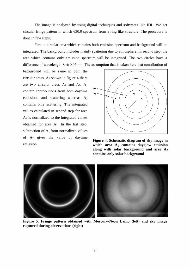
The image is analyzed by using digital techniques and softwares like IDL. We get

circular fringe pattern in which 630.0 spectrum from a ring like structure. The procedure is

done in few steps;

First, a circular area which contains both emission spectrum and background will be

integrated. The background includes mainly scattering due to atmosphere. In second step, the

area which contains only emission spectrum will be integrated. The two circles have a

difference of wavelength λ=± 0.05 nm. The assumption that is taken here that contribution of

background will be same in both the

circular areas. As shown in figure 4 there

are two circular areas A1 and A2. A1

contain contributions from both daytime

emissions and scattering whereas A2

contains only scattering. The integrated

values calculated in second step for area

A2 is normalized to the integrated values

obtained for area A1. In the last step,

subtraction of A1 from normalized values

of A2 gives the value of daytime

emission.

Figure 5. Fringe pattern obtained with Mercury-Neon Lamp (left) and sky image

captured during observations (right)

Figure 4. Schematic diagram of sky image in

which area A1 contains dayglow emission

along with solar background and area A2

contains only solar background

12

6. Production mechanisms of dayglow

There are three different important emission lines recognized in which the emission line

at 630.0 nm is used extensively to study the dynamics of thermosphere worldwide. The

production mechanisms of these lines are presented here.

1. OI 557.7 nm or Oxygen Green Line

When transition of atomic oxygen from O(1S) to O(

1D) state takes place then we obtain

OI 557.7 nm emission line. There are a number of sources from which the emission arises;

they include electron impact, dissociative recombination, photo-dissociation of O2, and some

other chemical reactions.

Production of O(1S);

A. Photoelectrons (ep) which have sufficient energy are responsible for excitation O(1S)

and it is known as P E excitation,

O + ep O(1S) + ep

B. The N2 is excited due to impact of photoelectron and energy is transferred through

collision, known as Collisional deactivation of N2.

N2 + ep N2 (A3Σu

+)

N2 (A3Σu

+) + O N2 + O(

1S)

C. Photodissociation by the solar photons in the wavelength range of (90 nm - 120 nm),

O2 + hν O(1S) + O

D. Dissociative recombination takes place when O+

2 recombine with et to produce O(1D).

O+

2 + et O(1S) + O

E. In three-body recombination process an oxygen atom is excited to the O(1S) state by

the three body recombination with two other atoms.

O + O + O O2 + O(1S)

Loss of O(1S);

A. De-excitation by emitting photon known as radiative transition

O(1S) O(

1D) + hν (557.7 nm)

B. Collisional deactivation,

O(1D) + X O + X

2. OI 630.0 nm or Oxygen Red Line

The OI 630.0 nm emission is a result of transition from O(1D) to O(

3P) state.

13

Production of O(1D);

A. Photoelectron impact (PE) on the ground state oxygen, O (3P).

O(3P) + ep O(

1D) + e

B. Photodissociation (PD) of molecular oxygen in the Schumann-Runge continuum

(135-175 nm) of the solar radiation.

O2 + hν O(1D) + O(

3P)

C. Dissociative recombination (DR) of molecular oxygen ion.

O2+ + e O(

1D) + O(

3P)

Loss of O(1D);

A. Collisional quenching,

O(1D) + X O + X, where X may be N2, O2, O, or et

B. Radiative transition to red doublet:

O (1D) O + hν (630.0 nm, 636.4 nm)

3. OI 777.4 nm Line

When transition of O(5P) to O(

5S) state occur emission of this wavelength takes place.

Radiative recombination of O+ with electron gives rise to its excited state O(

5P),

O+ + e O(

5P)

The loss of O(5P) is through radiative transition,

O(5P) O(

5S) + hν (777.4 nm)

From the techniques described above, all these emissions as mentioned here can be

measured. A filter wheel type arrangement will be required. Further, the fringe pattern will be

different for different wavelengths. All these can be changed in an automated mode.

14

7. Summary

I worked in Space and Atmospheric Science Division of Physical Research Laboratory during

my internship. My work focused on both the theoretical and experimental aspects, to

understand the dynamics of thermosphere. In this project I studied about the different type of

techniques used to measure the dayglow emissions around the globe, problems associated

with them and dayglow photometer, an instrument which was developed at PRL.

15

8. Bibliography

1. Spectrophysics, Anne P. Thorne

2. Physics of the Aurora and Airglow, Joseph W. Chamberlain

3. Dayglow photometry: a new approach, Narayanan et al. (1989)

4. The First Daytime Ground-Based Optical image of the Aurora, Rees et al.

(2000)

5. Studies of Daytime Upper Atmospheric Phenomena Using Ground-Based

Optical Techniques, Prof. D. Pallamraju (1996)

6. Effects of Lower Atmospheric and Solar Forcings on Daytime Upper

Atmospheric Dynamics, Fazlul Islam Laskar (2015)