Paleo-constraints on future tropical Pacific climateKim M. Cobb

Pamela Grothe, Hussein Sayani, Alyssa Atwood, Tianran Chen, Intan NurhatiEarth and Atmospheric Sciences, Georgia Tech

Chris Charles, SIO, UCSDLarry Edwards, Hai Cheng, UMN

• Pa

leocli

mate R

esearch • Georgia Tech •

Cobb Lab

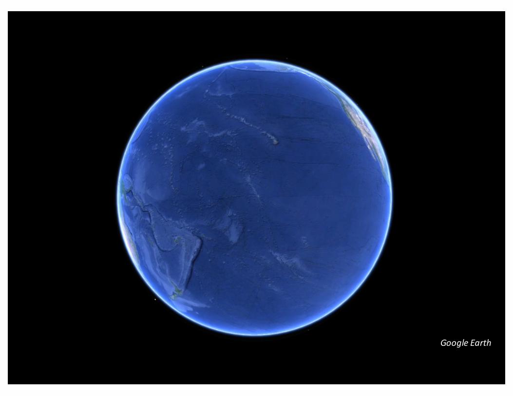
GoogleEarth

GoogleEarth

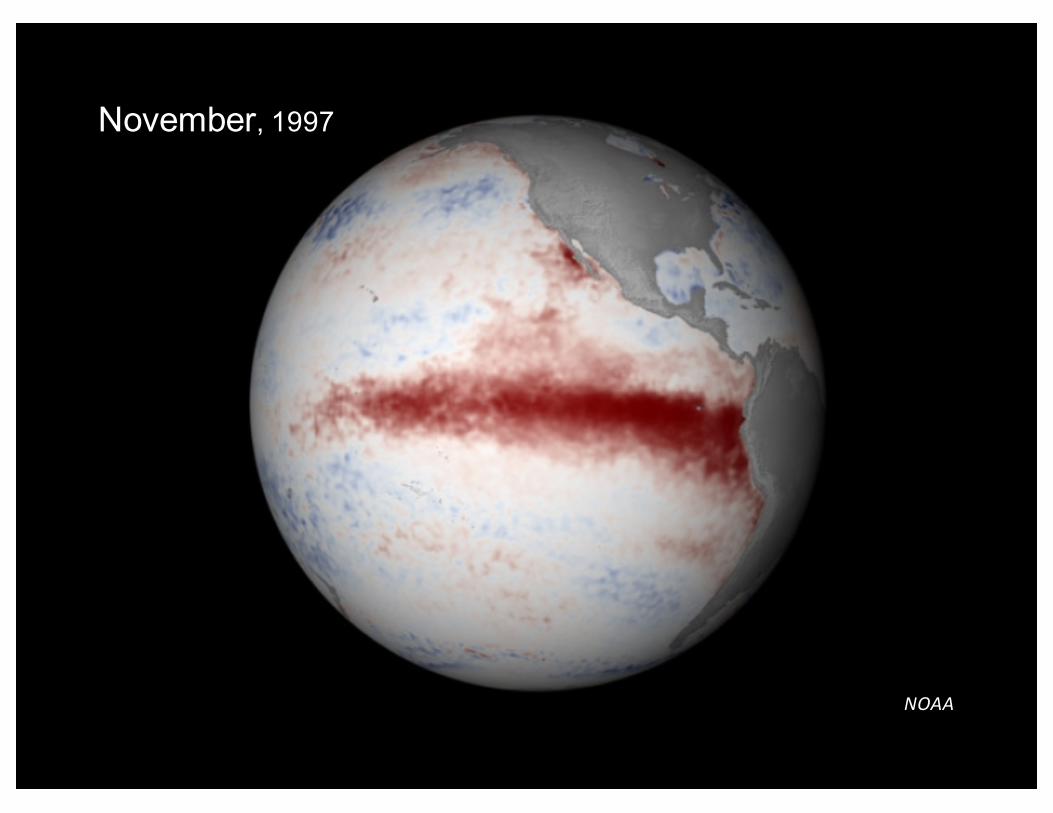
NOAA

November, 1997

https://socialforecasting.files.wordpress.com/2015/08/el-nino-godzilla.jpg

2015/2016 El Niño

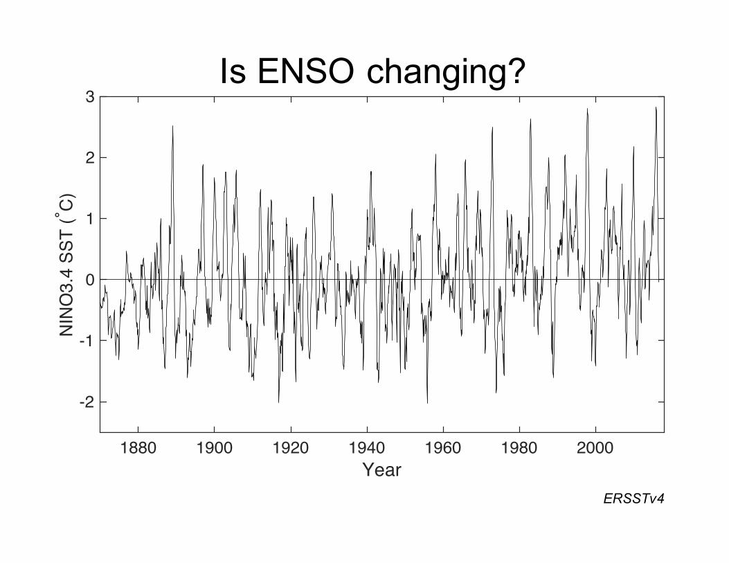
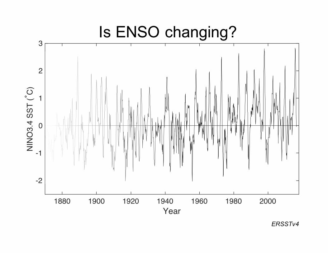
ERSSTv4

1880 1900 1920 1940 1960 1980 2000Year

-2

-1

0

1

2

3NI

NO3.

4 SS

T (° C)

Is ENSO changing?

ERSSTv4

1880 1900 1920 1940 1960 1980 2000Year

-2

-1

0

1

2

3NI

NO3.

4 SS

T (° C)

Is ENSO changing?

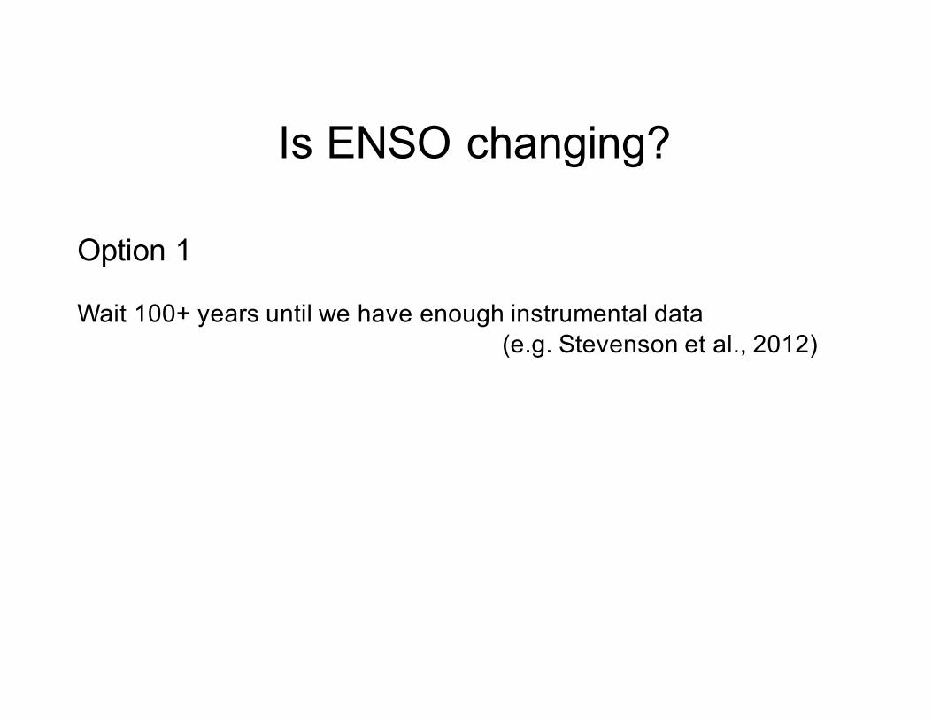
Option 1

Wait 100+ years until we have enough instrumental data(e.g. Stevenson et al., 2012)

Is ENSO changing?

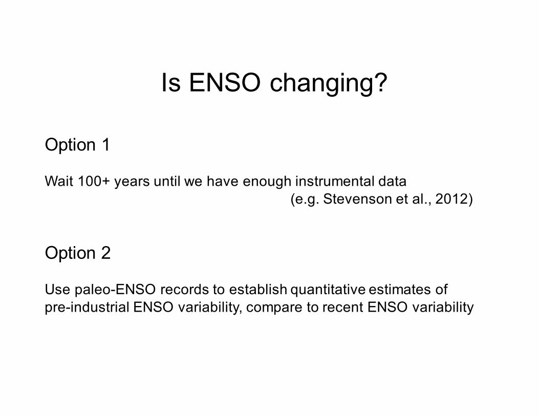
Option 1

Wait 100+ years until we have enough instrumental data(e.g. Stevenson et al., 2012)

Option 2

Use paleo-ENSO records to establish quantitative estimates of pre-industrial ENSO variability, compare to recent ENSO variability

Is ENSO changing?

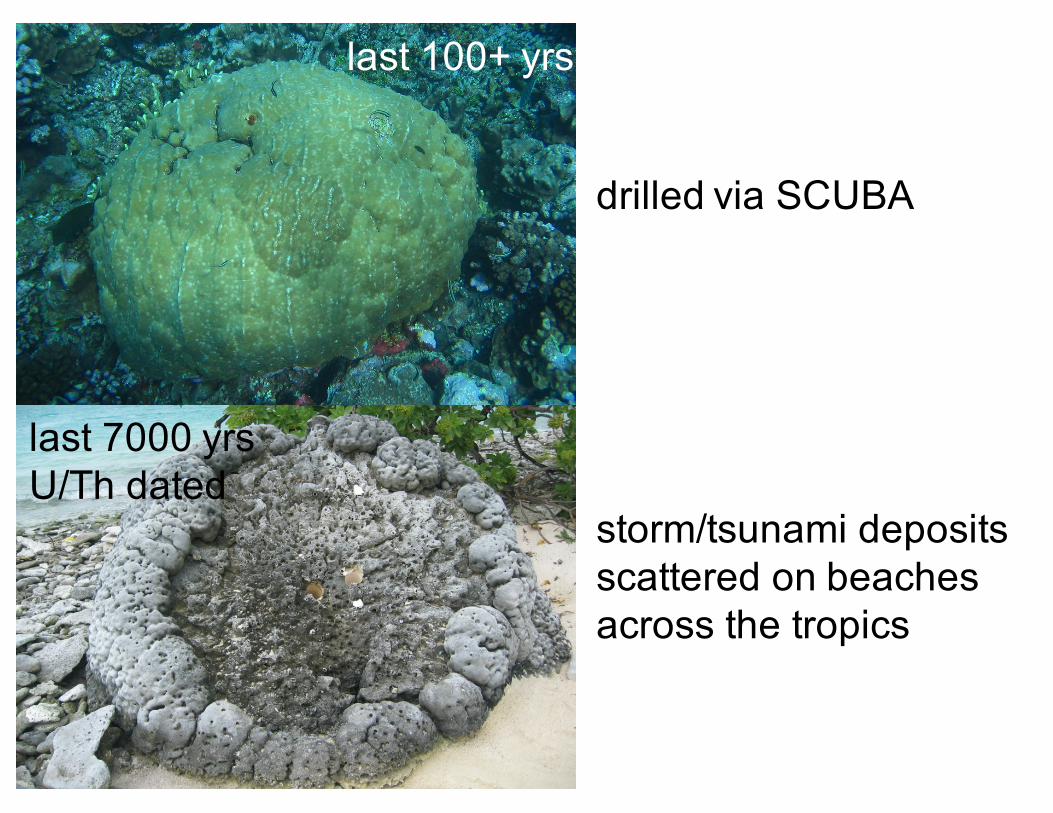
last 100+ yrs

last 7000 yrsU/Th dated

drilled via SCUBA

storm/tsunami depositsscattered on beachesacross the tropics

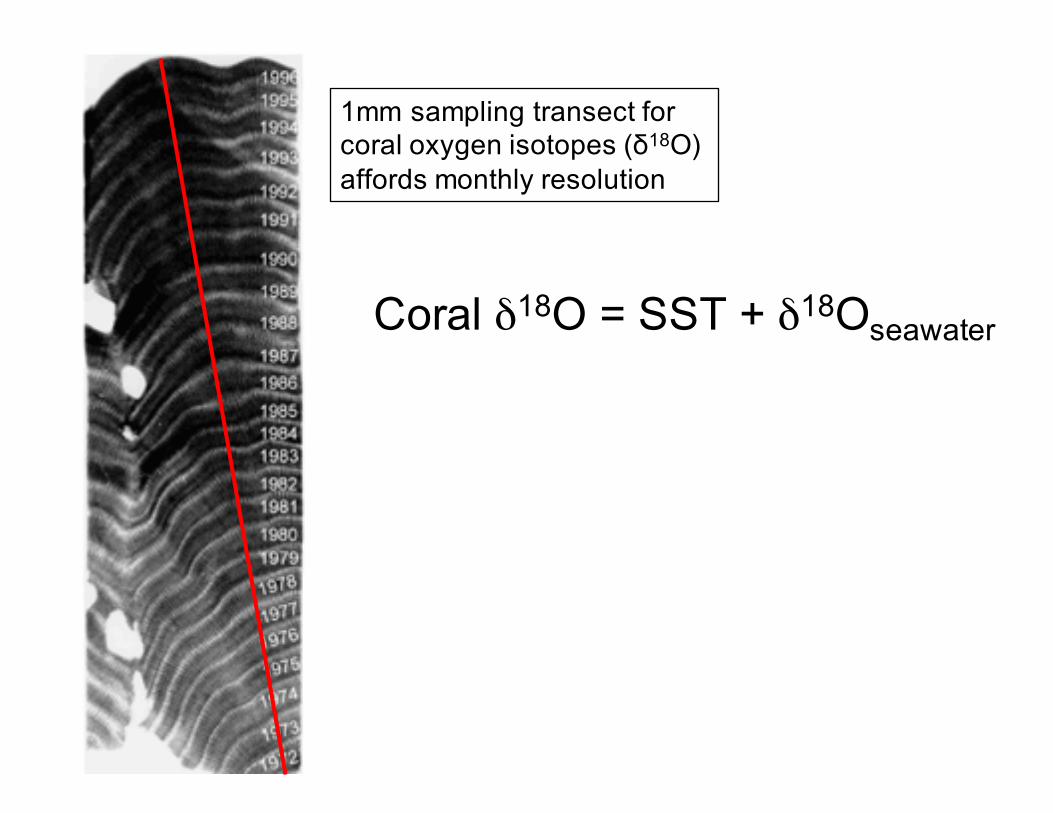
1mm sampling transect for coral oxygen isotopes (δ18O)affords monthly resolution

Coral δ18O = SST + δ18Oseawater

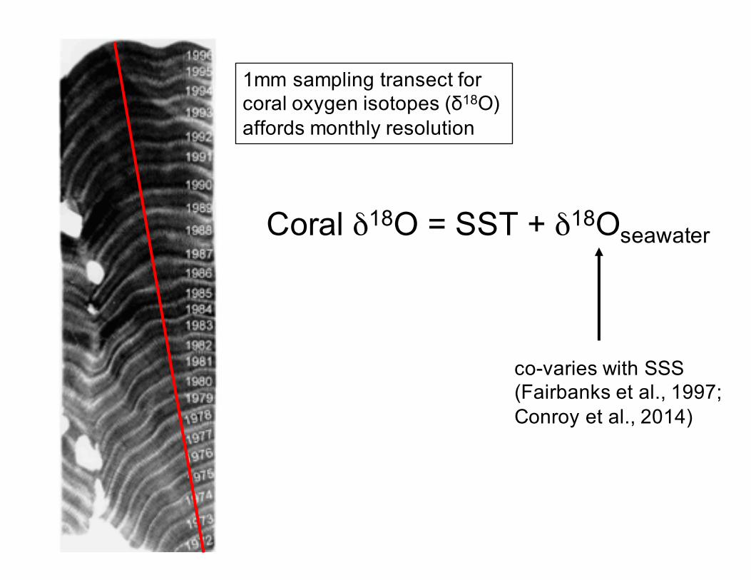
1mm sampling transect for coral oxygen isotopes (δ18O)affords monthly resolution

Coral δ18O = SST + δ18Oseawater

co-varies with SSS(Fairbanks et al., 1997;Conroy et al., 2014)

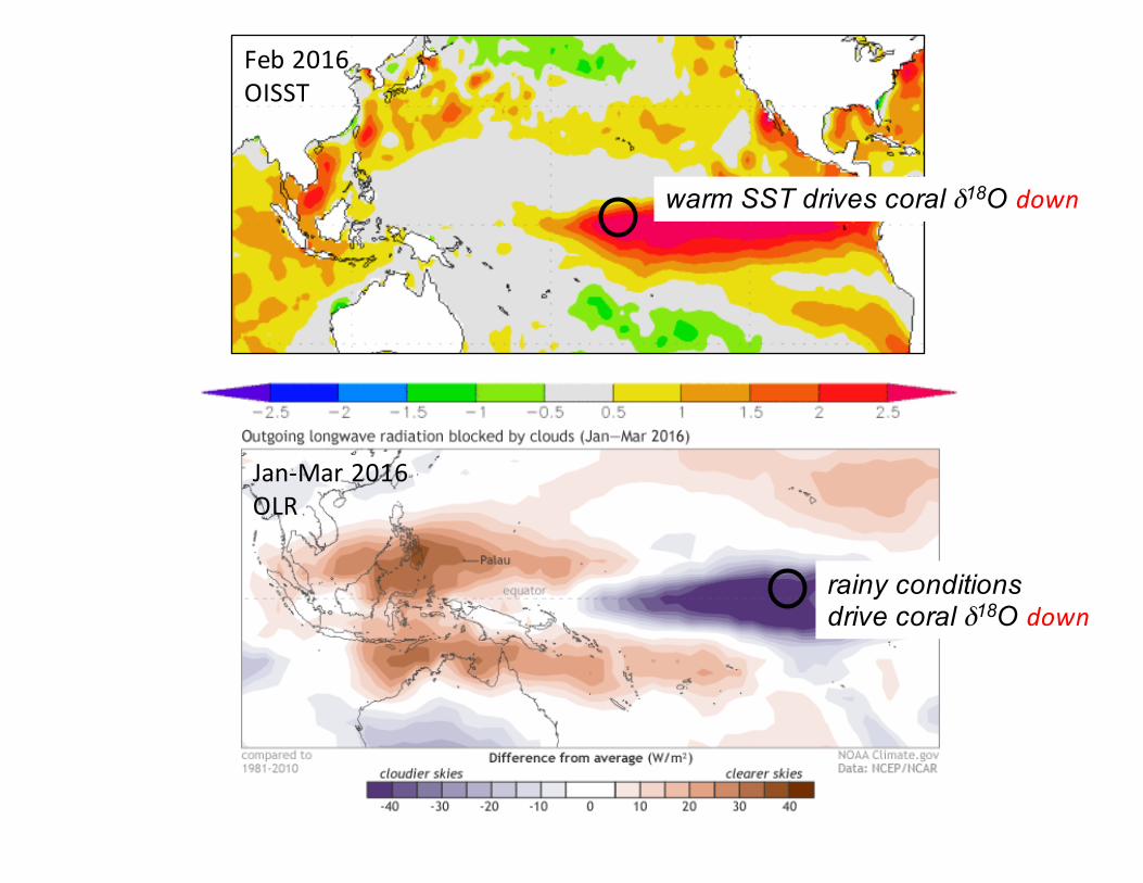
Feb2016

OISST

Jan-Mar2016

OLR

warm SST drives coral δ18O down

rainy conditionsdrive coral δ18O down

1970 1975 1980 1985 1990 1995 2000 2005 2010 2015

-5.5

-5

-4.5

-4

22

24

26

28

30

Nurhati09 Evans99 x126 x123 Minicore1 Minicore2 OISSTv2

SS

T (º

C)

δ18 O

(‰)

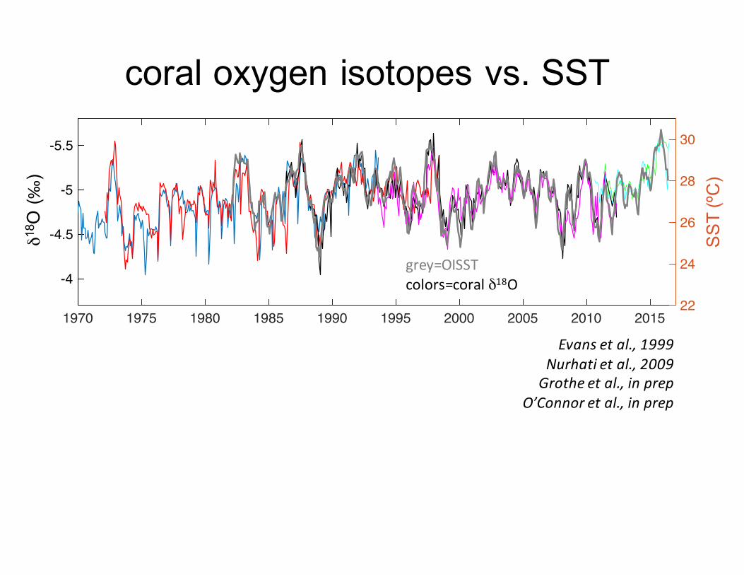
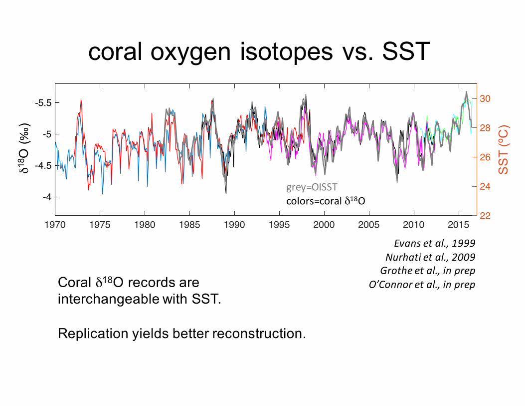
coral oxygen isotopes vs. SST

grey=OISST

colors=coralδ18O

Evansetal.,1999Nurhati etal.,2009Grothe etal.,inprep

O’Connoretal.,inprep

1970 1975 1980 1985 1990 1995 2000 2005 2010 2015

-5.5

-5

-4.5

-4

22

24

26

28

30

Nurhati09 Evans99 x126 x123 Minicore1 Minicore2 OISSTv2

SS

T (º

C)

δ18 O

(‰)

coral oxygen isotopes vs. SST

grey=OISST

colors=coralδ18O

Evansetal.,1999Nurhati etal.,2009Grothe etal.,inprep

O’Connoretal.,inprepCoral δ18O records are interchangeable with SST.

Replication yields better reconstruction.

800 1000 1200 1400 1600 1800 2000

−5.5

−5

−4.5

−4

Year CE

Xmas coral d18O last millennium

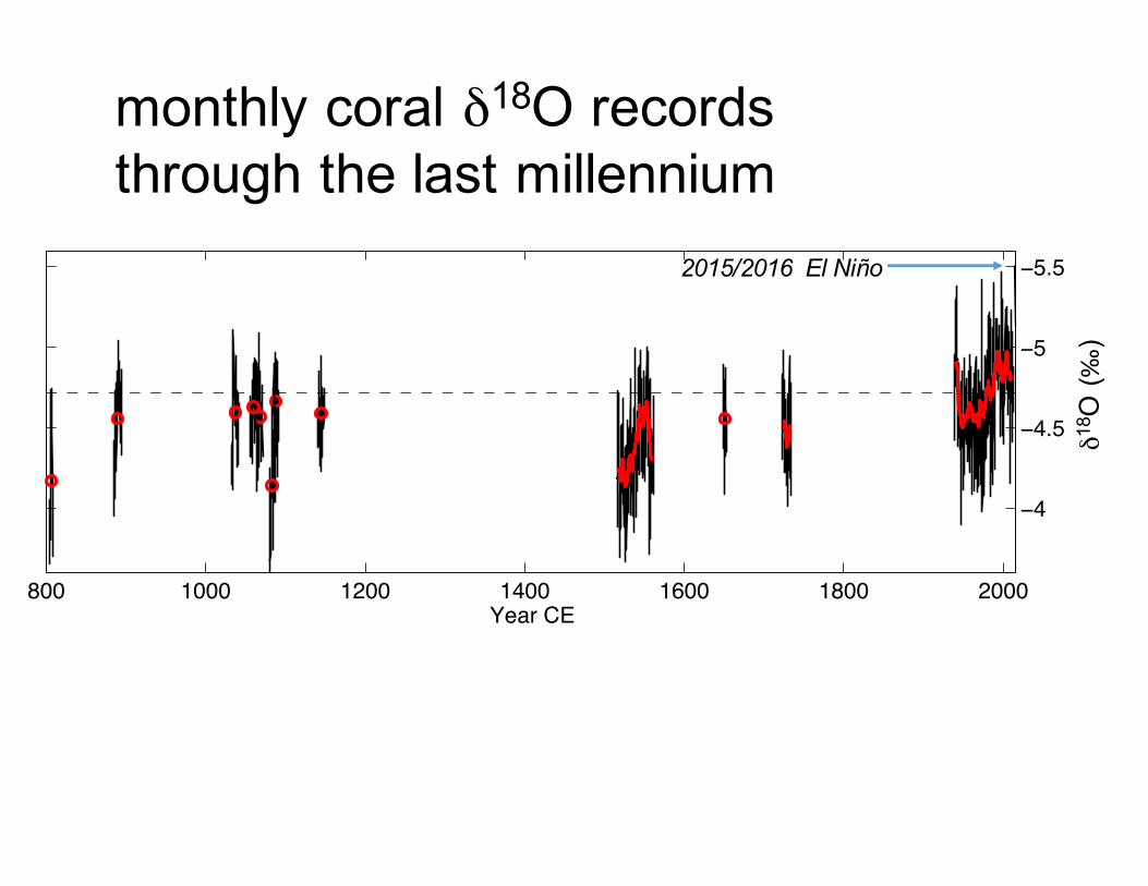
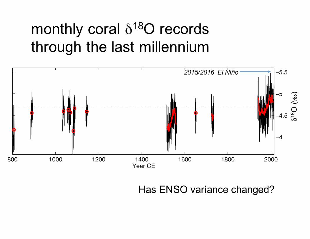
monthly coral δ18O recordsthrough the last millennium

2015/2016 El Niño

δ18 O

(‰)

800 1000 1200 1400 1600 1800 2000

−5.5

−5

−4.5

−4

Year CE

Xmas coral d18O last millennium

monthly coral δ18O recordsthrough the last millennium

2015/2016 El Niño

δ18 O

(‰)

Has ENSO variance changed?

01000200030004000500060007000

−60

−40

−20

0

20

40

Year BP

Cha

nge

in s

tdev

of E

NSO

(%)

Fanning

Christmas

Palmyra

20th century

range

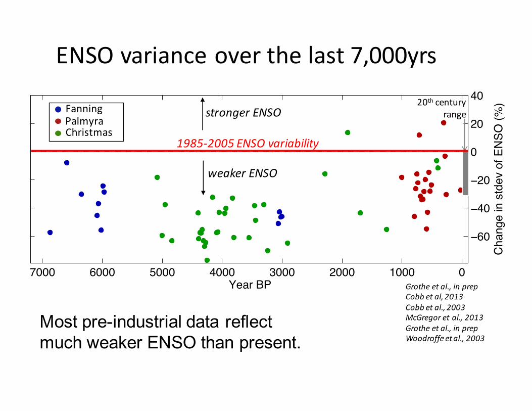
Grothe etal.,inprepCobbetal,2013Cobbetal.,2003McGregoretal.,2013Grothe etal.,inprepWoodroffe etal.,2003

1985-2005ENSOvariability

ENSOvarianceoverthelast7,000yrs

strongerENSO

weakerENSO

Most pre-industrial data reflectmuch weaker ENSO than present.

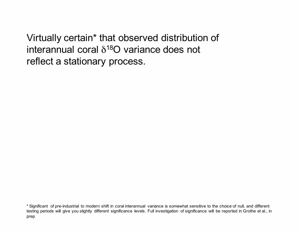
Virtually certain* that observed distribution ofinterannual coral δ18O variance does not reflect a stationary process.

* Significant of pre-industrial to modern shift in coral interannual variance is somewhat sensitive to the choice of null, and different testing periods will give you slightly different significance levels. Full investigation of significance will be reported in Grothe et al., in prep

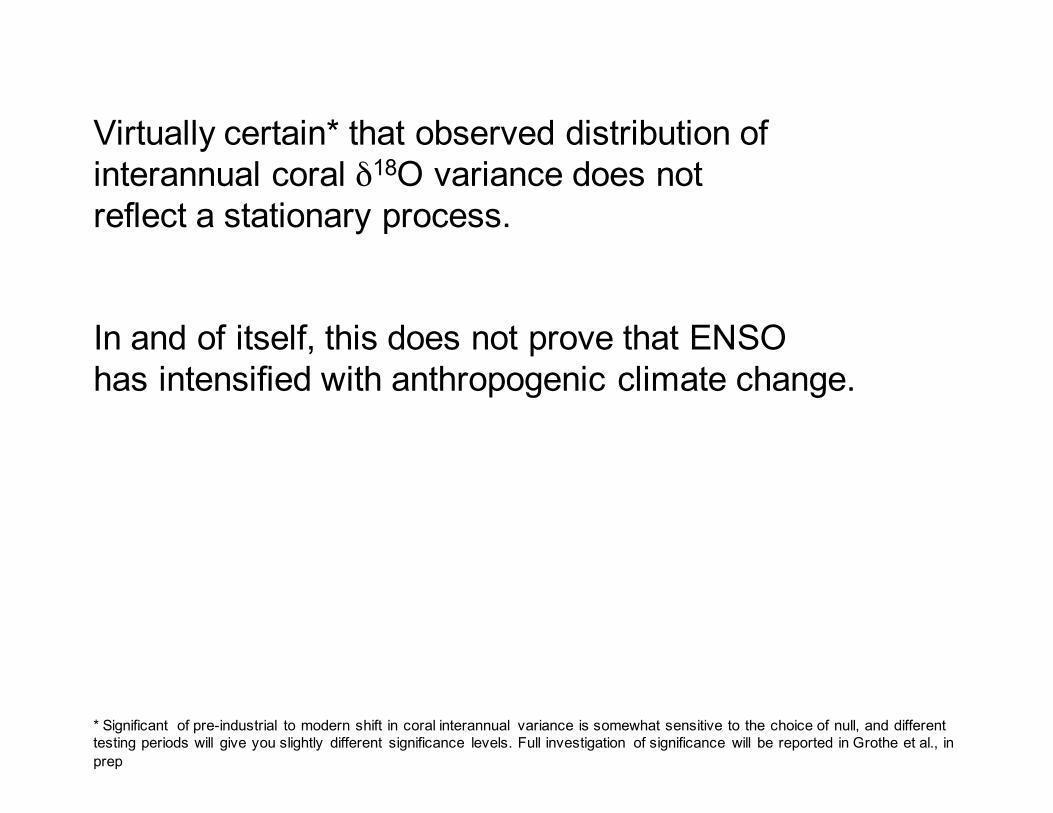
Virtually certain* that observed distribution ofinterannual coral δ18O variance does not reflect a stationary process.

In and of itself, this does not prove that ENSOhas intensified with anthropogenic climate change.

* Significant of pre-industrial to modern shift in coral interannual variance is somewhat sensitive to the choice of null, and different testing periods will give you slightly different significance levels. Full investigation of significance will be reported in Grothe et al., in prep

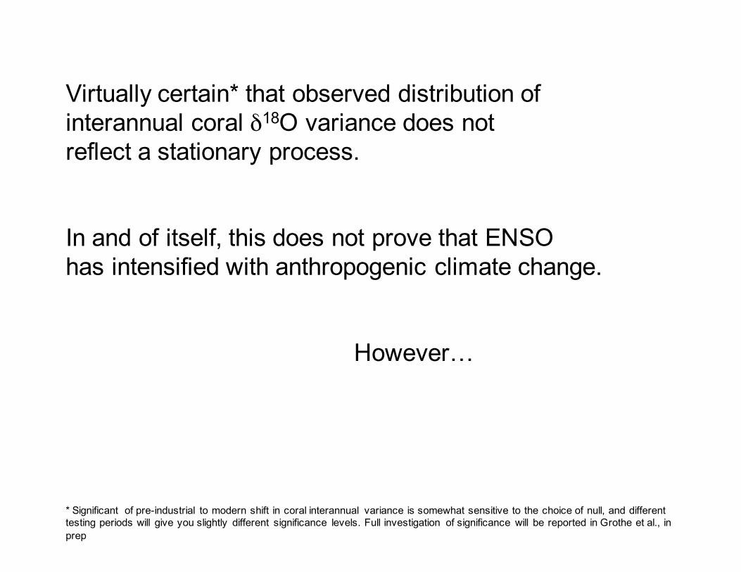
Virtually certain* that observed distribution ofinterannual coral δ18O variance does not reflect a stationary process.

In and of itself, this does not prove that ENSOhas intensified with anthropogenic climate change.

However…

* Significant of pre-industrial to modern shift in coral interannual variance is somewhat sensitive to the choice of null, and different testing periods will give you slightly different significance levels. Full investigation of significance will be reported in Grothe et al., in prep

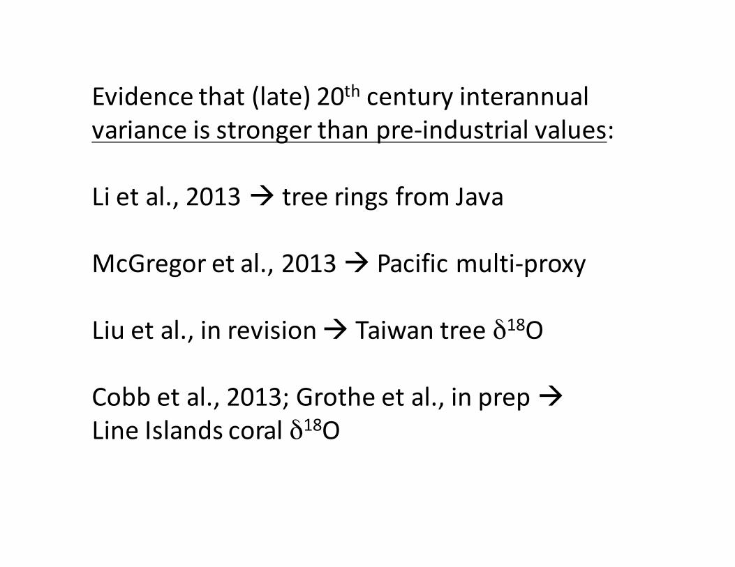
Evidencethat(late)20th centuryinterannual

varianceisstrongerthanpre-industrialvalues:

Lietal.,2013à treeringsfromJava

McGregoretal.,2013à Pacificmulti-proxy

Liuetal.,inrevisionà Taiwantreeδ18O

Cobbetal.,2013;Grothe etal.,inprepàLineIslandscoralδ18O

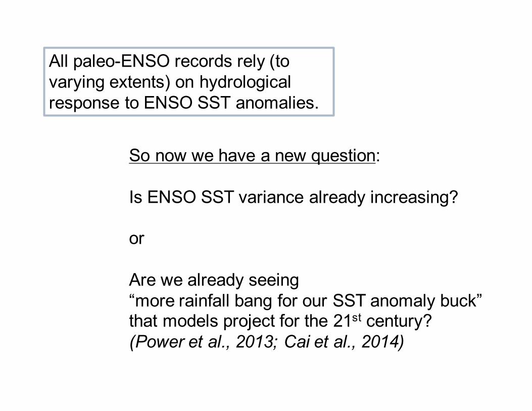
All paleo-ENSO records rely (to varying extents) on hydrological response to ENSO SST anomalies.

So now we have a new question:

Is ENSO SST variance already increasing?

or

Are we already seeing “more rainfall bang for our SST anomaly buck” that models project for the 21st century?(Power et al., 2013; Cai et al., 2014)

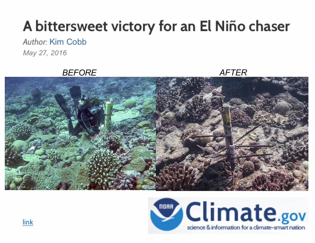
BEFORE AFTER

link

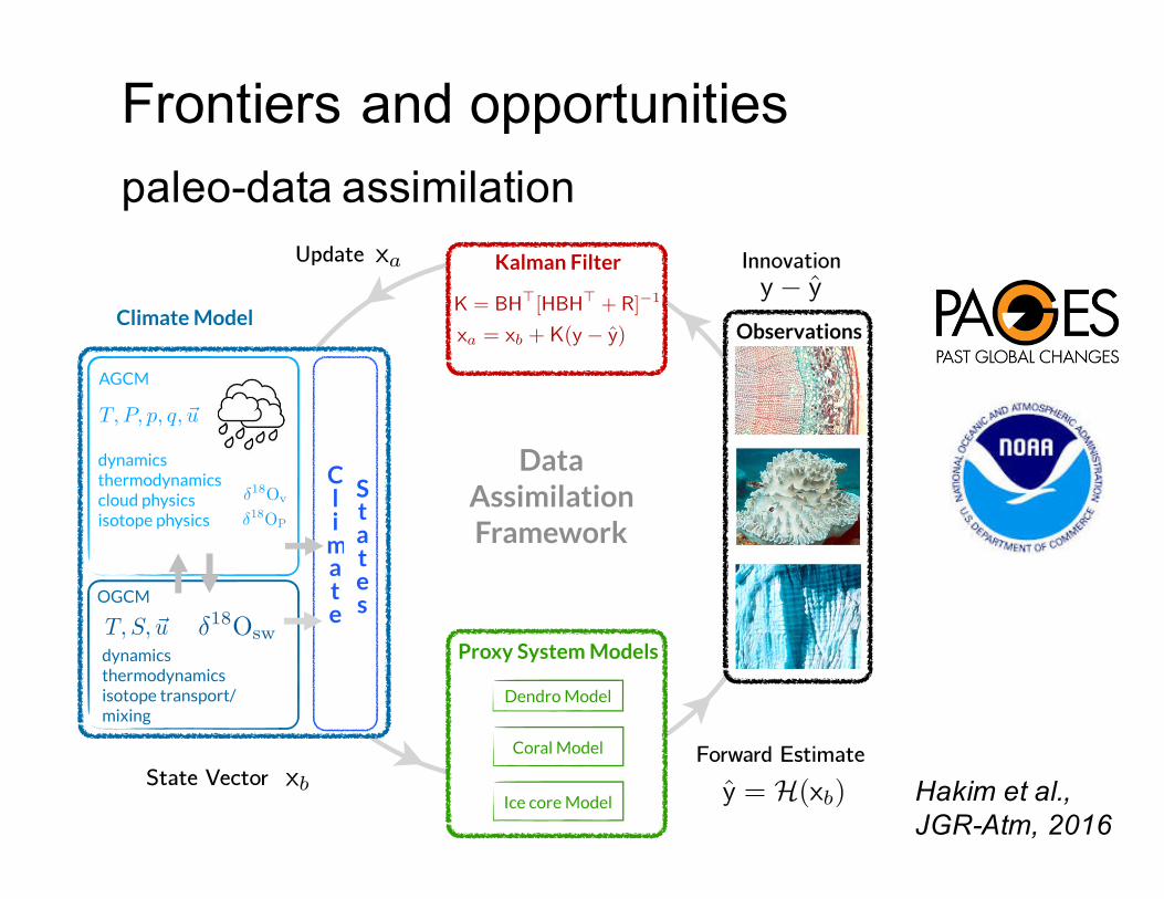
Frontiers and opportunitiespaleo-data assimilation

Journal of Geophysical Research: Atmospheres 10.1002/2016JD024751

Figure 1. Conceptual framework for the Last Millennium Reanalysis, outlining our paleoassimilation approach. Startingfrom the prior (a collection of simulated climate states) from which random draws are pulled, the states are mappedto proxy space via a proxy system model (PSM). These predictions y are compared to the actual proxy measurements yto compute the innovation, y − y. These innovations are then used to update the prior via the Kalman filter equations,which also update the error covariance. The cycle is repeated many (104) times to sample the distribution of the priorensemble.

diagonal matrix, and the diagonal values represent the error variance for each proxy (defined in section 2.4).A 100-member ensemble is used, and results are insensitive to this choice provided that the ensemble has atleast 50 members.

As an explicit illustration of how multivariate fields are recovered, consider a single tree ring width proxymeasurement for 1 year and assume a PSM that depends only on 2 m air temperature. We take the prior toconsist of 2 m air temperature at the location of the proxy and a globally gridded 500 hPa geopotential heightfield. The prior fields consist of an ensemble of annual-mean values, randomly drawn from a long climatesimulation. From this, we should expect that the prior estimate of the proxy, (xp), will differ considerablyfrom the proxy value; i.e., the innovation will be large. How much weight the innovation gets in equation (1)depends on R (see equation (2)), which in this example is simply a scalar variance, r. Given the innovation,which in this case is a scalar value, K determines the weight and transfers information from the innovation(in units of tree ring width) to the 500 hPa geopotential height field. Consider the 500 hPa geopotential heightat a single point in the global grid and call it x. From (2),

BHT ∼ 1n − 1

x(Hxp)T (3)

where n is the ensemble size and x is a row vector containing the ensemble of n values of 500 hPa geopo-tential heights (x) at the point, with the ensemble mean removed. The right side of equation (3) representsthe covariance between the 500 hPa height at the point and the prior estimate of the proxy. In the denomi-nator of K, HBHT is a scalar, representing the variance of the ensemble estimate of the proxy, var(ye) (directlycomparable to r). Therefore, we update the ensemble mean 500 hPa geopotential height at the point by

xa = xp + cov(xp, ye)var(ye) + r

(y − ye) (4)

where ye =Hxp is the prior estimated proxy; i.e., this equation says that the analysis 500 hPa geopotentialheight at the point is determined by linearly regressing the prior estimate against the innovation.

HAKIM ET AL. LAST MILLENNIUM REANALYSIS 6748

Hakim et al., JGR-Atm, 2016

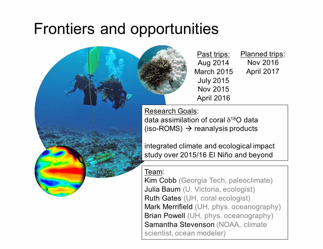
Past trips:

Aug 2014

March 2015

July 2015

Nov 2015

April 2016

Team:

Kim Cobb (Georgia Tech, paleoclimate)

Julia Baum (U. Victoria, ecologist)

Ruth Gates (UH, coral ecologist)

Mark Merrifield (UH, phys. oceanography)

Brian Powell (UH, phys. oceanography)

Samantha Stevenson (NOAA, climate

scientist, ocean modeler)

Planned trips:

Nov 2016

April 2017

Research Goals:

data assimilation of coral δ18O data

(iso-ROMS) à reanalysis products

integrated climate and ecological impact

study over 2015/16 El Niño and beyond

Frontiers and opportunities

Summary

The paleoclimate community needs CLIVARto unlock the vast potential of their data.

Summary

The paleoclimate community needs CLIVARto unlock the vast potential of their data.

CLIVAR needs the paleoclimate communityto address some of the most pressingquestions concerning the impacts of anthropogenic climate change.

Summary

The paleoclimate community needs CLIVARto unlock the vast potential of their data.

CLIVAR needs the paleoclimate communityto address some of the most pressingquestions concerning the impacts of anthropogenic climate change.

Rapid progress is possible but requires interdisciplinary teams of scientistsworking towards shared goals.