Grid design in estuaries and lagoons

using Delft3D Flexible Mesh

Bas van Maren, Arnold van Rooijen, Arthur van Dam,

Giselle Lemos (Technital), Herman Kernkamp

10 november 2014

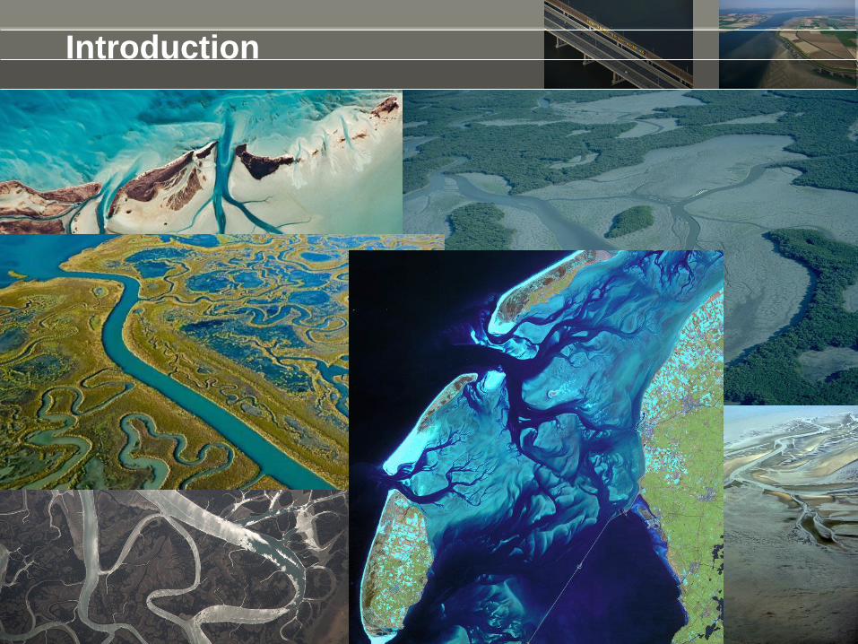
Introduction

Introduction

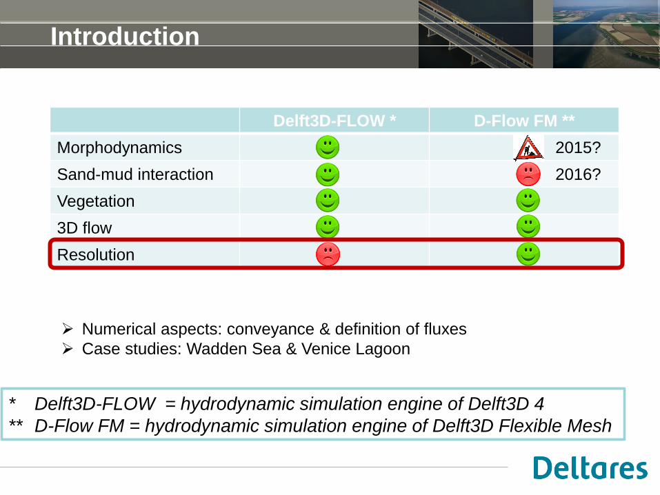
Delft3D-FLOW * D-Flow FM **

Morphodynamics 2015?

Sand-mud interaction 2016?

Vegetation

3D flow

Resolution

Numerical aspects: conveyance & definition of fluxes

Case studies: Wadden Sea & Venice Lagoon

* Delft3D-FLOW = hydrodynamic simulation engine of Delft3D 4

** D-Flow FM = hydrodynamic simulation engine of Delft3D Flexible Mesh

Model resolution

This presentation:

- Short introduction on computational methods in D-Flow FM related

to model resolution (conveyance and 2nd order fluxes)

- Comparison of D-Flow FM – Delft3D-FLOW, for two lagoons:

- Wadden Sea

- Venice Lagoon

5

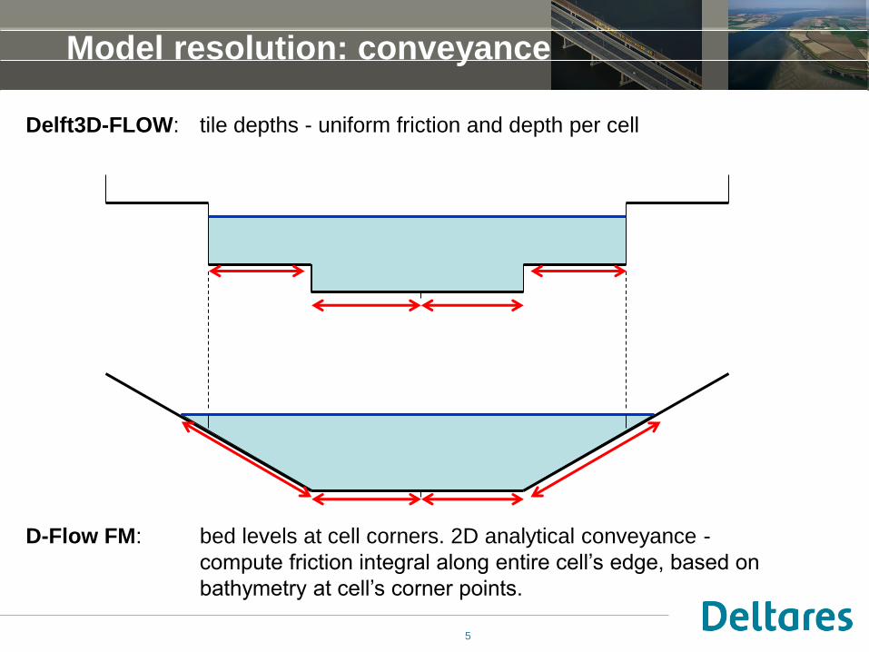
Delft3D-FLOW: tile depths - uniform friction and depth per cell

D-Flow FM: bed levels at cell corners. 2D analytical conveyance -

compute friction integral along entire cell’s edge, based on

bathymetry at cell’s corner points.

Model resolution: conveyance

KfKI, Bremerhaven, 2 November 2011 6

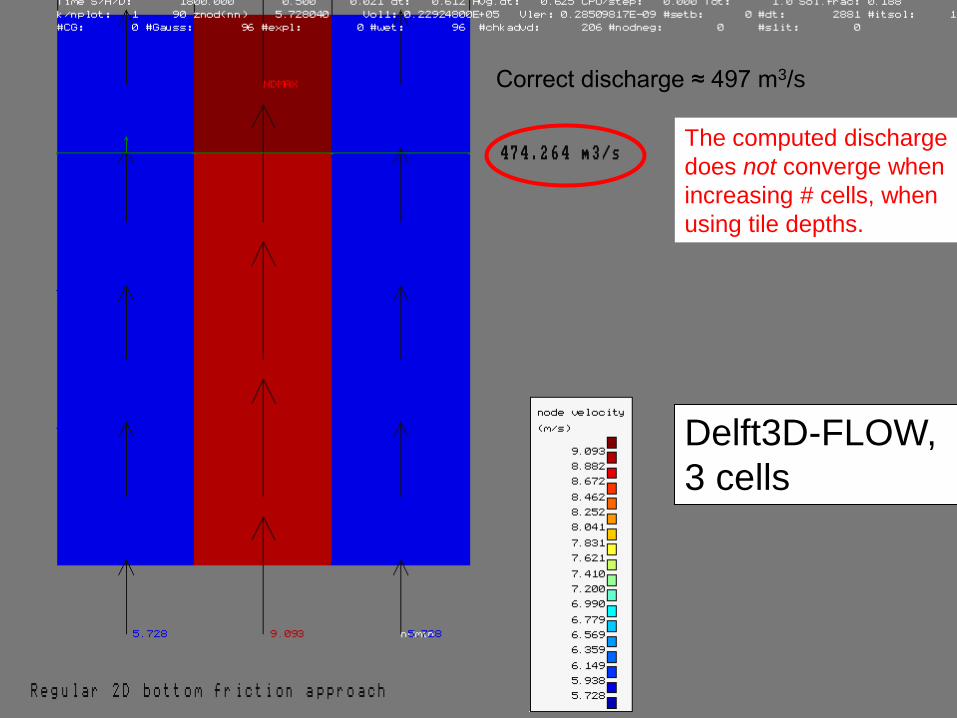
Delft3D-FLOW,

3 cells

The computed discharge

does not converge when

increasing # cells, when

using tile depths.

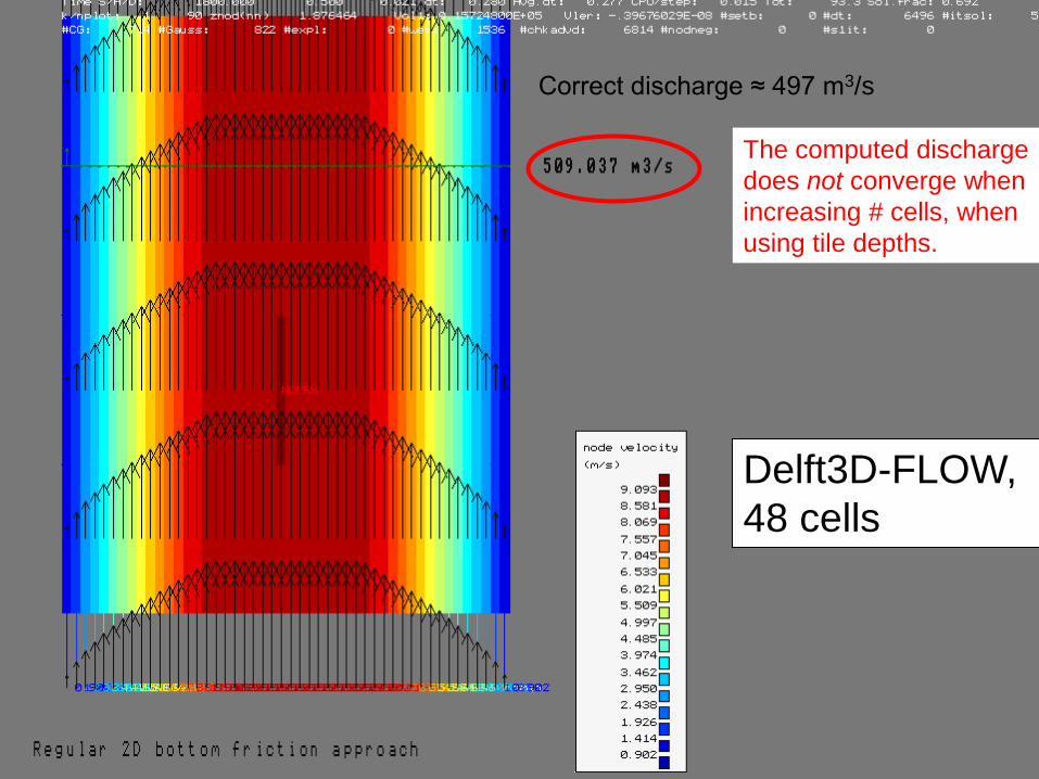
Correct discharge ≈ 497 m3/s

KfKI, Bremerhaven, 2 November 2011 7

The computed discharge

does not converge when

increasing # cells, when

using tile depths.

Correct discharge ≈ 497 m3/s

Delft3D-FLOW,

48 cells

KfKI, Bremerhaven, 2 November 2011 8

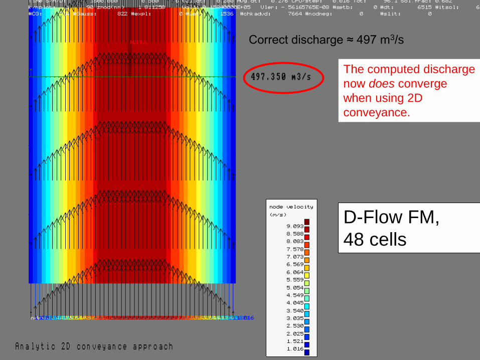
The computed discharge

now does converge

when using 2D

conveyance.

Correct discharge ≈ 497 m3/s

D-Flow FM,

48 cells

KfKI, Bremerhaven, 2 November 2011 9

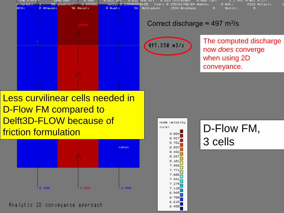
The computed discharge

now does converge

when using 2D

conveyance.

Correct discharge ≈ 497 m3/s

D-Flow FM,

3 cells

Less curvilinear cells needed in

D-Flow FM compared to

Delft3D-FLOW because of

friction formulation

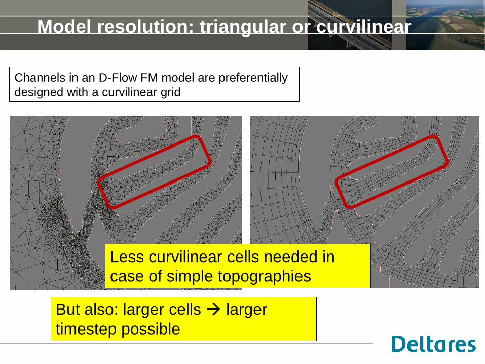
Model resolution: triangular or curvilinear

Less curvilinear cells needed in

case of simple topographies

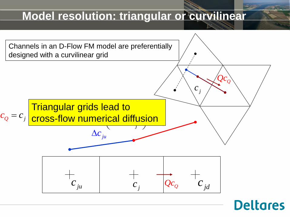
Channels in an D-Flow FM model are preferentially

designed with a curvilinear grid

But also: larger cells larger

timestep possible

QQc

QQc

juc

jdcjcjuc

1

12

,ju

j

j jQ

j

j

u tc c S

xc cc

jc

jc

Triangular grids lead to

cross-flow numerical diffusion

Model resolution: triangular or curvilinear

Channels in an D-Flow FM model are preferentially

designed with a curvilinear grid

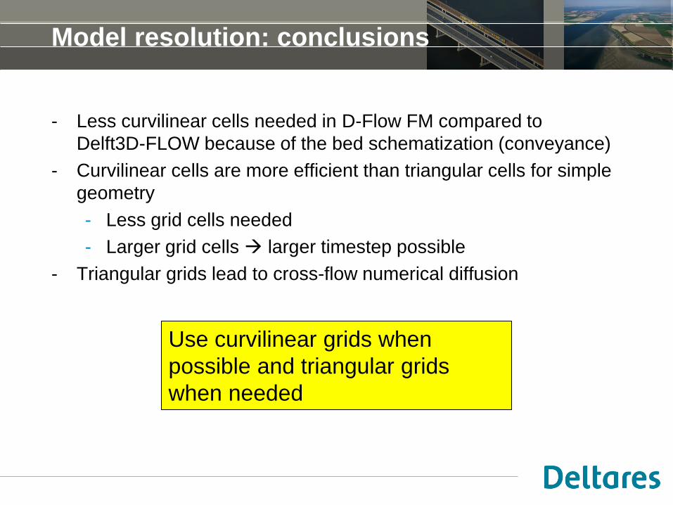
Model resolution: conclusions

- Less curvilinear cells needed in D-Flow FM compared to

Delft3D-FLOW because of the bed schematization (conveyance)

- Curvilinear cells are more efficient than triangular cells for simple

geometry

- Less grid cells needed

- Larger grid cells larger timestep possible

- Triangular grids lead to cross-flow numerical diffusion

Use curvilinear grids when

possible and triangular grids

when needed

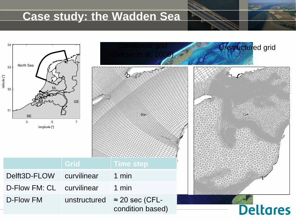
Case study: the Wadden Sea

Curvilinear grid

(Borsje et al. 2008) Unstructured grid

Grid Time step

Delft3D-FLOW curvilinear 1 min

D-Flow FM: CL curvilinear 1 min

D-Flow FM unstructured ≈ 20 sec (CFL-

condition based)

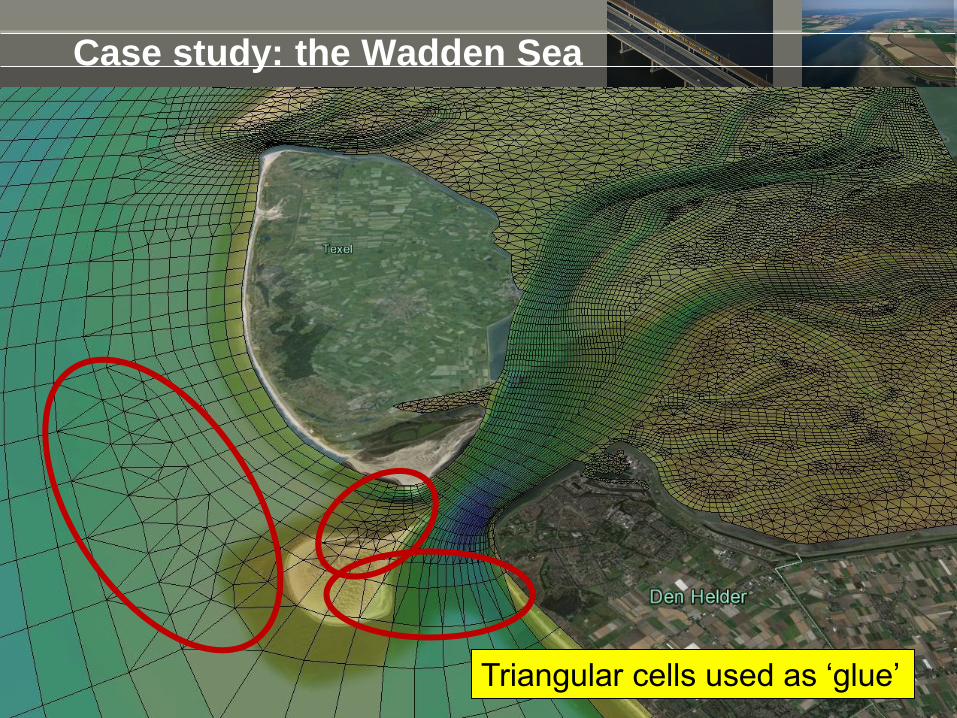
Case study: the Wadden Sea

10 november 2014

Triangular cells used as ‘glue’

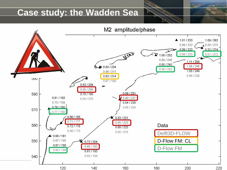
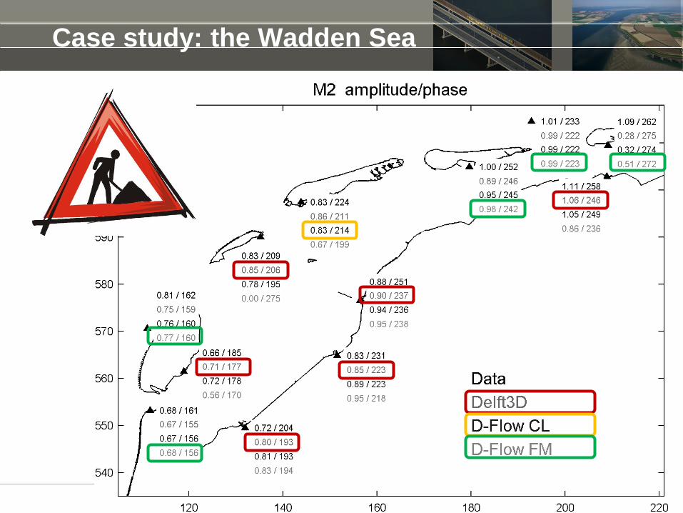
Case study: the Wadden Sea

Delft3D-FLOW

D-Flow FM: CL

D-Flow FM

Data

Case study: the Wadden Sea

10 november 2014

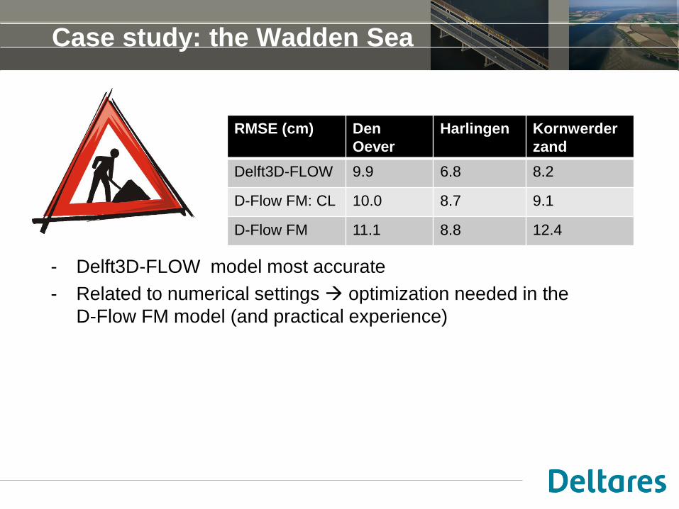
Case study: the Wadden Sea

- Delft3D-FLOW model most accurate

- Related to numerical settings optimization needed in the

D-Flow FM model (and practical experience)

RMSE (cm) Den

Oever

Harlingen Kornwerder

zand

Delft3D-FLOW 9.9 6.8 8.2

D-Flow FM: CL 10.0 8.7 9.1

D-Flow FM 11.1 8.8 12.4

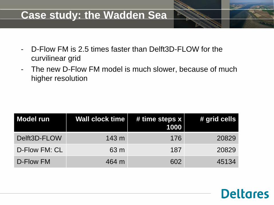
Case study: the Wadden Sea

- D-Flow FM is 2.5 times faster than Delft3D-FLOW for the

curvilinear grid

- The new D-Flow FM model is much slower, because of much

higher resolution

Model run Wall clock time # time steps x

1000

# grid cells

Delft3D-FLOW 143 m 176 20829

D-Flow FM: CL 63 m 187 20829

D-Flow FM 464 m 602 45134

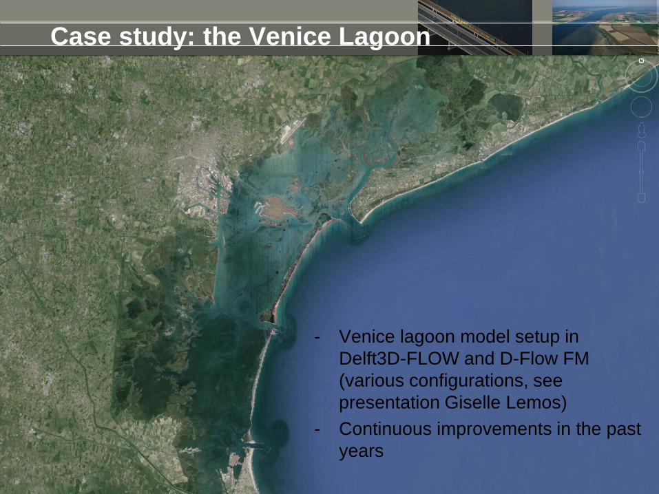
Case study: the Venice Lagoon

- Venice lagoon model setup in

Delft3D-FLOW and D-Flow FM

(various configurations, see

presentation Giselle Lemos)

- Continuous improvements in the past

years

Case study: the Venice Lagoon

10 november 2014

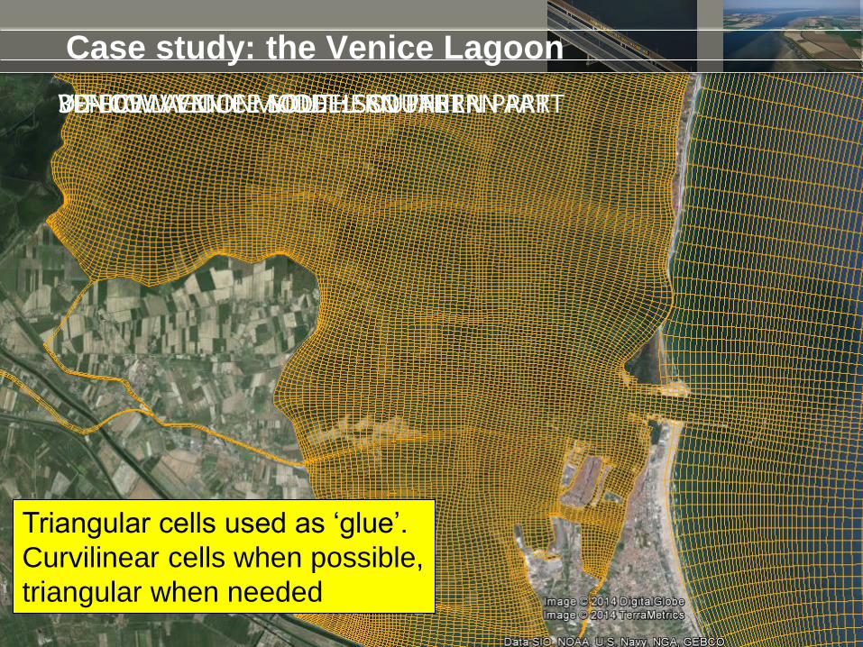
VENICE LAGOON: SOUTHERN PART 3D-FLOW VENICE MODEL: SOUTHERN PART D-FLOW VENICE MODEL: SOUTHERN PART

Triangular cells used as ‘glue’.

Curvilinear cells when possible,

triangular when needed

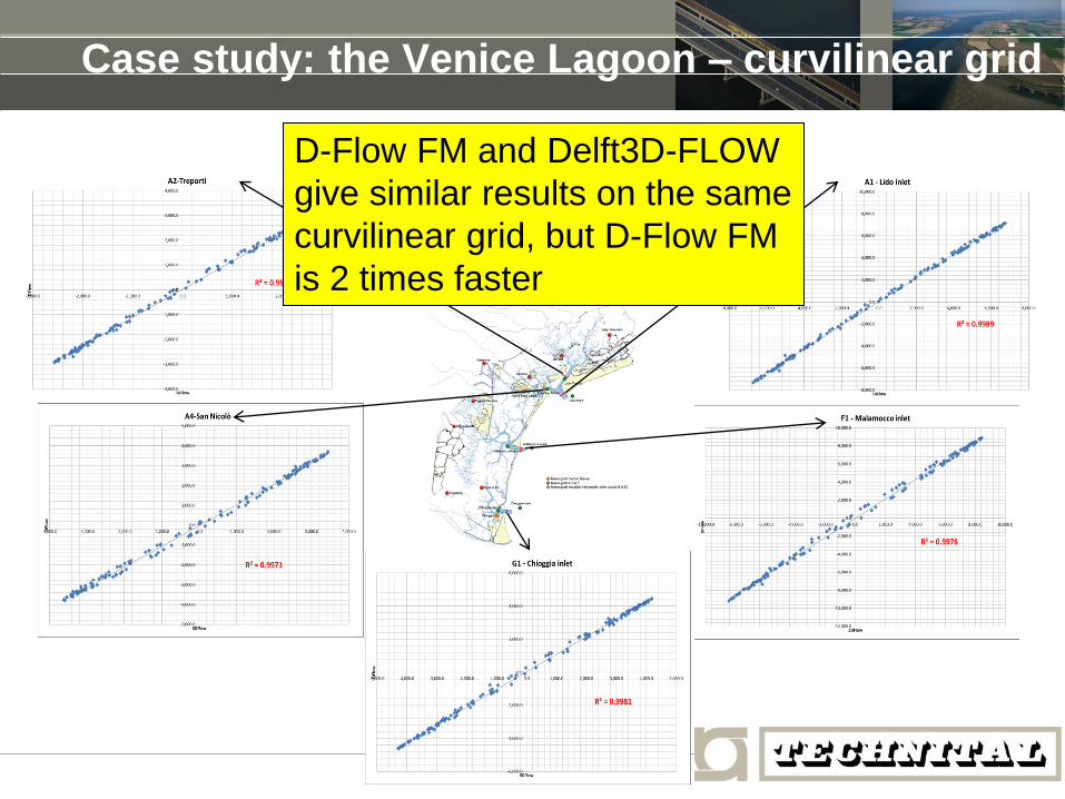
Case study: the Venice Lagoon – curvilinear grid

10 november 2014

D-Flow FM and Delft3D-FLOW

give similar results on the same

curvilinear grid, but D-Flow FM

is 2 times faster

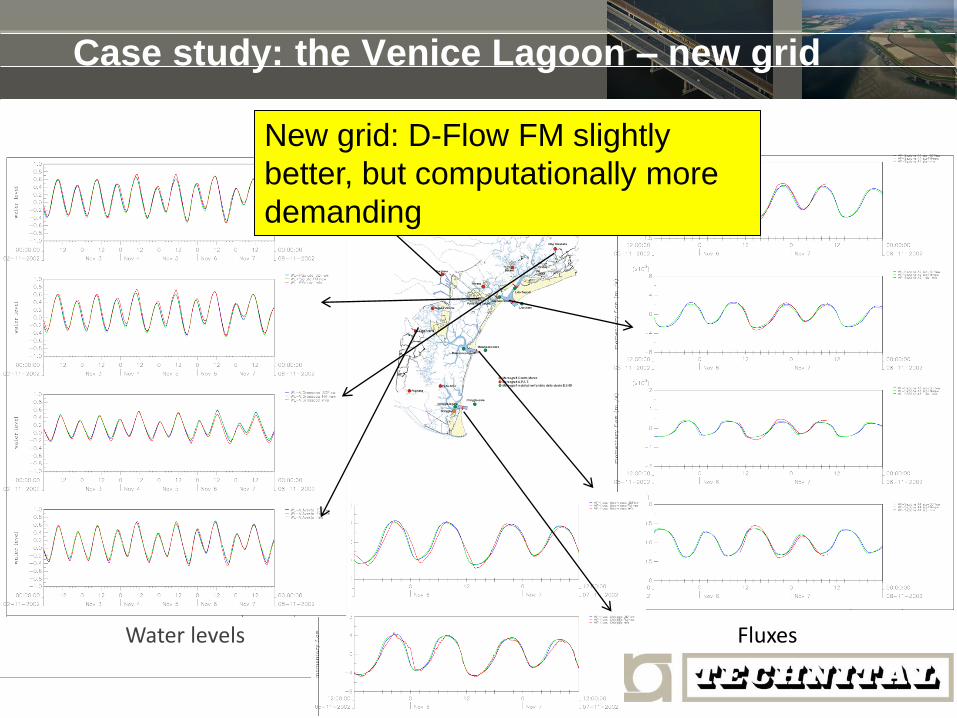
Case study: the Venice Lagoon – new grid

Fluxes Water levels

New grid: D-Flow FM slightly

better, but computationally more

demanding

Conclusions

D-Flow FM is more accurate in complex topographies less grid

cells required

D-Flow FM is faster combined with less grid cells the model should

be much faster

Case studies: D-Flow FM is >2 times faster on same curvilinear grid

and comparably accurate

Pitfall: increase the horizontal resolution (too much…) resulting in

(much) slower models

Setting up an D-Flow FM grid takes time – think carefully before actual

grid design

Need to improve hands-on experience for accurate numerical settings

Use curvilinear grids when possible and triangular grids when needed

(‘glue’)