Computationally Efficient Protocols to

Evaluate the Fatigue Resistance of Polycrystalline Materials

Noah H. Paulson, Matthew W. Priddy, Surya R. Kalidindi, and

David L. McDowell

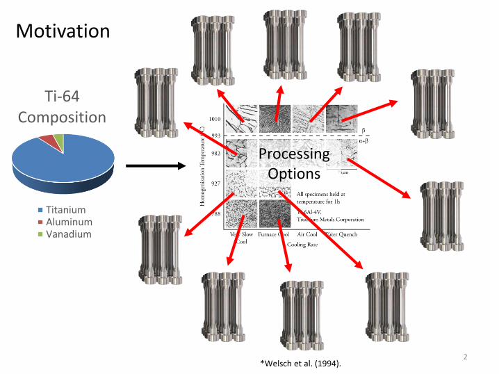
Motivation

*Welsch et al. (1994).

Processing Options

2

Ti-64Composition

TitaniumAluminumVanadium

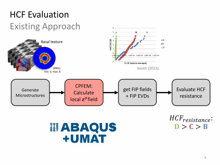
Generate Microstructures

CPFEM: Calculate

local 𝜺𝑝field

get FIP fields + FIP EVDs

Evaluate HCF resistance

HCF EvaluationExisting Approach

Smith (2013).

+UMAT

𝐻𝐶𝐹𝑟𝑒𝑠𝑖𝑠𝑡𝑎𝑛𝑐𝑒:𝐃 > 𝐂 > 𝐁

(0001)min: 0, max: 8

Basal texture

3

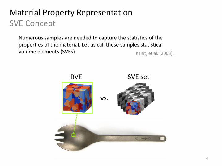
Material Property RepresentationSVE Concept

Kanit, et al. (2003).

Numerous samples are needed to capture the statistics of the properties of the material. Let us call these samples statistical volume elements (SVEs)

4

RVE SVE set

vs.

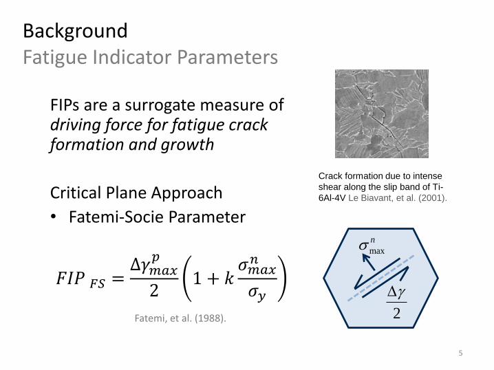
BackgroundFatigue Indicator Parameters

FIPs are a surrogate measure of driving force for fatigue crack formation and growth

Critical Plane Approach

• Fatemi-Socie Parameter

𝐹𝐼𝑃 𝐹𝑆 =∆𝛾𝑚𝑎𝑥

𝑝

21 + 𝑘

𝜎𝑚𝑎𝑥𝑛

𝜎𝑦

max

n

2

Crack formation due to intense

shear along the slip band of Ti-

6Al-4V Le Biavant, et al. (2001).

5

Fatemi, et al. (1988).

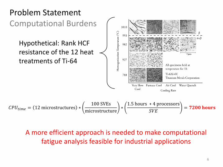
Problem StatementComputational Burdens

Hypothetical: Rank HCF resistance of the 12 heat treatments of Ti-64

𝐶𝑃𝑈𝑡𝑖𝑚𝑒 = 12 microstructures ∗100 SVEs

microstructure∗

1.5 hours ∗ 4 processors

𝑆𝑉𝐸= 𝟕𝟐𝟎𝟎 𝐡𝐨𝐮𝐫𝐬

A more efficient approach is needed to make computational fatigue analysis feasible for industrial applications

6

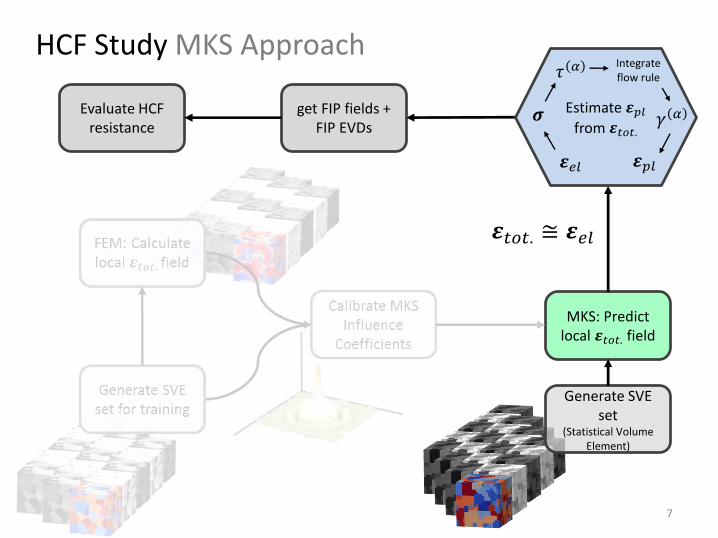
HCF Study MKS Approach

MKS: Predict local 𝜺𝑡𝑜𝑡. field

Generate SVE set

(Statistical Volume Element)

get FIP fields + FIP EVDs

Evaluate HCF resistance

Estimate 𝜺𝑝𝑙from 𝜺𝑡𝑜𝑡.

𝜺𝑒𝑙

𝝈

𝜏 𝛼 Integrate flow rule

𝛾 𝛼

𝜺𝑝𝑙

𝜺𝑡𝑜𝑡. ≅ 𝜺𝑒𝑙

7

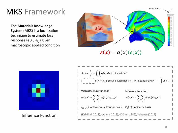
The Materials Knowledge System (MKS) is a localization technique to estimate local response (e.g., 𝜀𝑖𝑗) given

macroscopic applied condition

MKS Framework

𝜺 𝒙

𝜺 𝑥 = 𝑰 − 𝑅

𝐻

𝜶 𝑟, 𝑛 𝑚 𝑥 + 𝑟, 𝑛 𝑑𝑛𝑑𝑟

+ 𝑅

𝑅

𝐻

𝐻

𝜶 𝑟, 𝑟′, 𝑛, 𝑛′ 𝑚 𝑥 + 𝑟, 𝑛 𝑚 𝑥 + 𝑟 + 𝑟′, 𝑛′ 𝑑𝑛𝑑𝑛′𝑑𝑟𝑑𝑟′ −⋯ 𝜺 𝑥

𝑚 𝑥, 𝑛 =

𝐿

𝑠

𝑀𝑠𝐿𝑄𝐿(𝑛)𝑋𝑠(𝑥)

Microstructure function:

𝜶 𝑟, 𝑛 =

𝐿

𝑡

𝑨𝑡𝐿𝑄𝐿 𝑛 𝜒𝑡 𝑟

Influence function:

𝑄𝐿 𝑛 : orthonormal Fourier basis 𝑋𝑠(𝑥): indicator basis

(Kalidindi 2012), (Adams 2012), (Kröner 1986), Yabansu (2014)

𝜺 𝒙 = 𝒂 𝒙 𝜺 𝒙

Influence Function

8

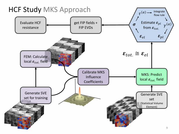
HCF Study MKS Approach

MKS: Predict local 𝜺𝑡𝑜𝑡. field

Generate SVE set

(Statistical Volume Element)

get FIP fields + FIP EVDs

Evaluate HCF resistance

Calibrate MKS Influence

Coefficients

Generate SVE set for training

FEM: Calculate local 𝜺𝑡𝑜𝑡. field

Estimate 𝜺𝑝𝑙from 𝜺𝑡𝑜𝑡.

𝜺𝑒𝑙

𝝈

𝜏 𝛼 Integrate flow rule

𝛾 𝛼

𝜺𝑝𝑙

𝜺𝑡𝑜𝑡. ≅ 𝜺𝑒𝑙

9

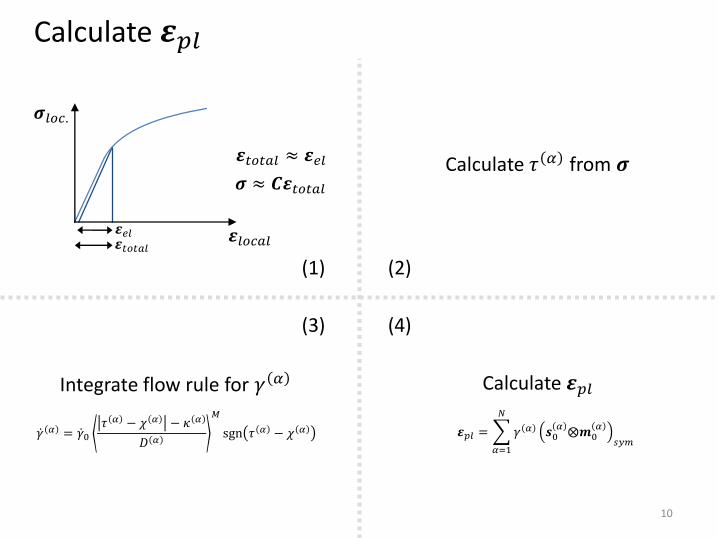
𝜺𝑝𝑙 =

𝛼=1

𝑁

𝛾 𝛼 𝒔0𝛼⨂𝒎0

𝛼

𝑠𝑦𝑚

Calculate 𝜺𝑝𝑙

Calculate 𝜺𝑝𝑙

Calculate 𝜏 𝛼 from 𝝈

𝜺𝑙𝑜𝑐𝑎𝑙

𝝈𝑙𝑜𝑐.

𝜺𝑒𝑙𝜺𝑡𝑜𝑡𝑎𝑙

𝜺𝑡𝑜𝑡𝑎𝑙 ≈ 𝜺𝑒𝑙

𝝈 ≈ 𝑪𝜺𝑡𝑜𝑡𝑎𝑙

𝛾 𝛼 = 𝛾0𝜏 𝛼 − 𝜒 𝛼 − 𝜅 𝛼

𝐷 𝛼

𝑀

sgn 𝜏 𝛼 − 𝜒 𝛼

Integrate flow rule for 𝛾 𝛼

(1) (2)

(3) (4)

10

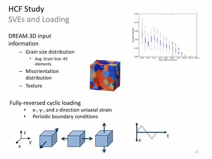
HCF StudySVEs and Loading

DREAM.3D input information

– Grain size distribution• Avg. Grain Size: 43

elements

– Misorientation distribution

– Texture

xy

z

εt

Fully-reversed cyclic loading• x-, y-, and z-direction uniaxial strain• Periodic boundary conditions

11

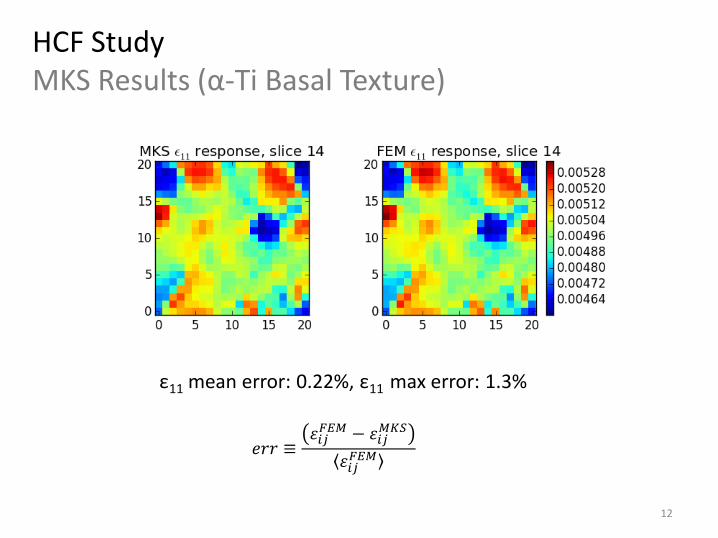
HCF StudyMKS Results (α-Ti Basal Texture)

ε11 mean error: 0.22%, ε11 max error: 1.3%

𝑒𝑟𝑟 ≡𝜀𝑖𝑗𝐹𝐸𝑀 − 𝜀𝑖𝑗

𝑀𝐾𝑆

𝜀𝑖𝑗𝐹𝐸𝑀

12

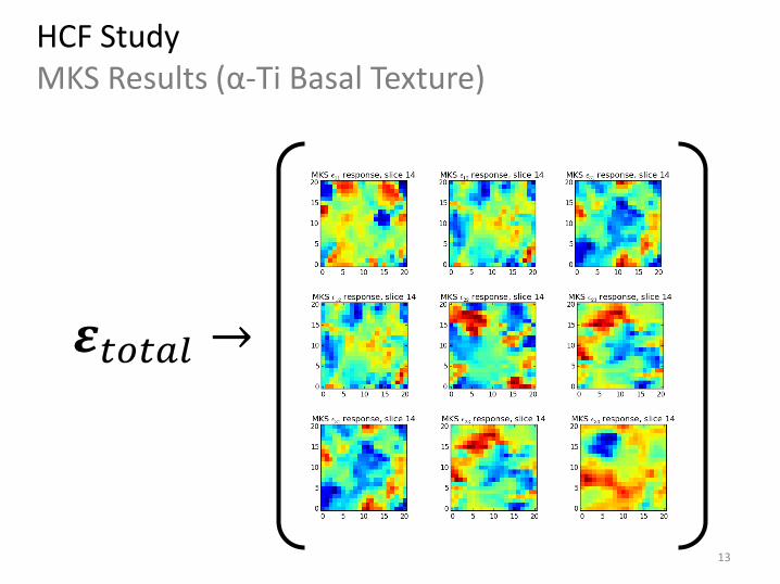
HCF StudyMKS Results (α-Ti Basal Texture)

𝜺𝑡𝑜𝑡𝑎𝑙 →

13

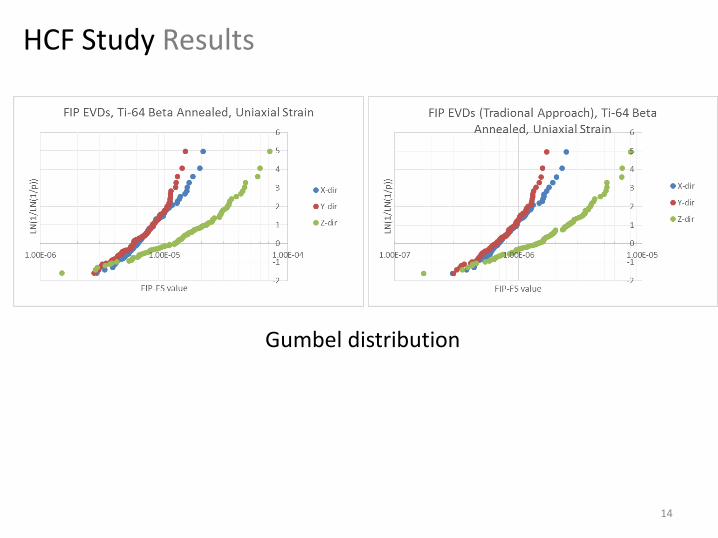
HCF Study Results

14

Gumbel distribution

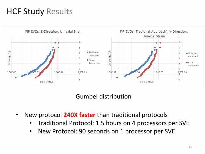
HCF Study Results

15

Gumbel distribution

• New protocol 240X faster than traditional protocols• Traditional Protocol: 1.5 hours on 4 processors per SVE• New Protocol: 90 seconds on 1 processor per SVE

• Protocols have been developed to evaluate the HCF and LCF resistance of polycrystalline materials

𝛾 𝛼 = 𝛾 𝛼 𝜏 𝛼 , 𝜺𝑝𝑙 =

𝛼=1

𝑁

𝛾 𝛼 𝑷 𝛼

• HCF Study: New protocol 240X faster than traditional protocols

HCF/LCF StudyConclusions

16

Acknowledgements

Also thanks to Donald S. Shih (Boeing), Yuksel C. Yabansu(GT), Dipen Patel (GT), and David Brough (GT)

GOALIFunding provided by:

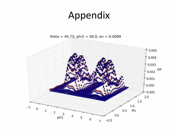
Appendix

References

• Alharbi HF, Kalidindi SR. Int J Plasticity 2015;66:71.

• Adams BL, Kalidindi SR, Fullwood DT. Microstructure Sensitive Design for Performance Optimization: Elsevier Science, 2012.

• Bunge HJ, Moris PR. Texture Analysis in Materials Science: Butterworth & Co, 1982

• Fast T, Kalidindi SR. Acta Mater 2011;59:4595.

• Kalidindi SR. ISRN Mater Sci 2012;2012:13.

• Kröner E. J Mech Phy Solids 1977;25:137.

• Landi G, Niezgoda SR, Kalidindi SR. Acta Mater 2010;58:2716.

• Przybyla C., Prasannavenkatesan R., Salajegheh N., McDowell D.L. Microstructure-sensitive modeling of high cycle fatigue. International Journal of Fatigue, Vol. 32, Iss. 3, (2010) pg. 512-525

• Przybyla C.P., McDowell D.L. Simulation-based extreme value marked correlations in fatigue of advanced engineering alloys. Procedia Engineering, Vol. 2, Iss. 1, (2010) pg. 1045-1056

• Smith BD. Masters Thesis 2013.

• Yabansu YC, Patel DK, Kalidindi SR. Acta Mater 2014;81:151.

19