Buyer-Vendor Integrated system – the Technique of EOQ Dependent Shipment Size to Achieve Steady Level and Cost Minimization

IOSR Journal of Mathematics (IOSR-JM)

e-ISSN: 2278-5728,p-ISSN: 2319-765X, 6, Issue 6 (May. - Jun. 2013), PP 46-57 www.iosrjournals.org

www.iosrjournals.org 46 | Page

Buyer-Vendor Integrated system – the Technique of EOQ

Dependent Shipment Size to Achieve Steady Level and Cost

Minimization

Dr. Pradeep .j.jha L.J. Institute of engineering and technology

Abstract: Study of buyer-vendor integrated system, in general, has two major features; determining delivery

schedule with supply quantity in each shipment and minimization of total incremental cost. Researchers in this

area concentrate on latter part, which probably may not justify both the features.

Many models developed so far, without considering both the features, begin with some pre-determined shipment

pattern and establish cost minimization but may not establish stability in supply or shipment size that may vary

in reality. In fact along with cost minimization stability in shipment size should also be a dominant feature of the

doubly effective inventory model. Stable supply within a normal limit of small fluctuation will allow the carrying charges to be considered constant.

The importance of the model lies in making all shipment size dependent on EOQ. The shipment size gets stable

after two or three shipments and achieves optimization of total incremental cost.

I. Introduction: As mentioned in the abstract we confront with two major points; developing an organized policy for

determining size of each shipment along with shipment schedule, and minimization of total incremental cost.

Authors on the same line have analyzed these two points with different perspectives and approaches.

Mr. Banerjee (1986) is, as known so far, the first one to envisage and construct a mathematical model in the area

of integrated system. He examined the case as 'lot for lot' model. In this pattern, the manufacturer produces in a

separate batch the total requirement of each buyer. Forking away from this, Dr. Goyal (1988) tried to establish that the integral number of equal shipments in a production run produces the lower cost. His work assumed that

shipments should be done only upon the completion of total production that meets the buyer‘s requirement.

In the heuristic approach, Mr. Lu (1995) gave a solution to the problem of single vendor and multiple

buyers. He also made the same assumption of the integral number of equal shipments. Taking the same

example, Mr.Goyal (1995) tried to establish that making shipments with sequentially increasing size in each

successive shipment is more justifiable with the fundamental objectives. Once the size of the initial shipment is

determined then the size of successive shipments, as he planned, keeps on increasing by a constant factor. This

factor was the ratio of production rate (P) to the demand rate (d).

On the top of this, Mr. Roger Hill (1996) tried to establish that not this factor (P/d) but some other

constant number in the range (1, P/d); could play a better role in minimizing the total incremental cost.

The problem is to unfold the approach of finding this constant number. Any algorithm working for the

search of this number, I think, should be satisfactory enough to justify his approach. Also in addition to the above point, the shipment sizes as derived by the above approach found to have incomparable and non-realistic

variations. In the example, as shown in his paper (Hill R.M. (1996)), establishes four shipments and the size of

the fourth shipment is ten times that of the first one!! This is not a realistic approach. It may be true theoretically

but fails in practical situations

The wide gaps between the number of units in the size of the first and each consecutive shipment,

unbalance the pattern of (i) transportation and (ii) inventory holding. It in turn becomes responsible in increasing

the incremental cost. As what found in reality, there are always slabs / intervals indicating minimum number of

units in the dispatch in the case of transportation or minimum amount of units in storage in the case of holding

the items of inventory. This is because of agencies dealing with such works have designed a pattern of

applying inventory holding charges depending on the number of units in each shipment. The holding charges

vary for different intervals. Any amount less than the upper limit of an internal is bound to generate an opportunity loss and

eventually increase the total incremental cost.

Also, any amount just more than the upper limit of an internal is subjected to the charge for the rate

applicable for that interval. In addition, the charges for the successive intervals keep on increasing. In

connection with this facts, if the shipment size increases at the rate P/d or by a number just greater than 1.5 then

it generates a wide gap between the size of successive shipments and eventually the estimates for the

incremental costs hardly match with that of in real life situation.

Buyer-Vendor Integrated system – The Technique of EOQ Dependent Shipment Size to Achieve Steady


Summing-up all the discussions above, and heading towards solution, it is recommended that shipment size

initially in first two or at the most three dispatches should moderately increase and then over the remaining

shipments should go steady. In addition, that too may not create a wide gap between the sizes of any two

shipments. This is the concept of "Promotional Increments."

II. Notations and Key-words: a. Notations: (1) i,j,n : Integer (positive) variables (Generally n > 3)

(2) P : Production Rate

(3) d : Demand Rate

(4) A1 : Set - up cost per unit time.

(5) A2 : Ordering Cost per order

(6) h1 : Holding Cost per unit per unit time for Vendor

(7) h2 : Holding Cost per unit per unit time for buyer (8) T : One cycle time.

(9) qs : Average inventory per unit time for the system.

(10) qB : Average inventory per unit time for the buyer.

(11) qV : Average inventory per unit time for the Vendor.

(12) TIC (q,n) Total Incremental Cost function.

(13) qj Basic shipment quantity for j = 1 to n

(14) n : Number of orders/ number of shipments (Decision

Variable)

Note:

Some notations like k1, k2, and k3 etc. are temporarily introduced which help deriving final results more easily;

they are well defined at the proper point of time.

3.2 Key-words:

(1) Basic quantity (2) Promotional Increments (3) Steady flow in shipment size

(4) Carrying cost (5) Total incremental cost (6) Inventory management

3.3 Assumptions: Assuming that the unknown factors affecting the system shall remain within control limits,

assumptions to substantiate the procedure of the model are as follows.

(1) The production rate and the demand rate are pre-known and remain constant.

(2) Shortages are not allowed. There is no lead time.

(3) Replenishment rate is instantaneous and infinite.

(4) Stock at the vendor's end at the time of supply is always greater than buyer's order size.

(5) The vendor and the buyer both begin their operations simultaneously at the onset of the cycle.

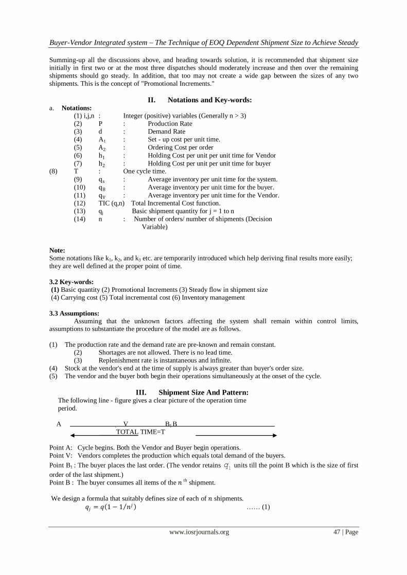
III. Shipment Size And Pattern: The following line - figure gives a clear picture of the operation time

period.

A V B1 B

TOTAL TIME=T

Point A: Cycle begins. Both the Vendor and Buyer begin operations.

Point V: Vendors completes the production which equals total demand of the buyers.

Point B1 : The buyer places the last order. (The vendor retains q1

units till the point B which is the size of first

order of the last shipment.)

Point B : The buyer consumes all items of the 𝑛 th shipment.

We design a formula that suitably defines size of each of 𝑛 shipments.

𝑞𝑗 = 𝑞 1 − 1 𝑛𝑗 …… (1)



[For a fixed n > 3 and j =1, 2, 3 …n]

From the above formula, we have

q q q qj n

j

n

1 2

1

....

=

= /jq d

2

1

( 1) 1/

1

nn

j

j

n n nq q

n

For greater value of n, 1 0/ nn and hence we ignore its contribution.

2

1

( 1)

1

n

j

j

n nq q

n

….… (2)

In connection of the time line above, different time-Slots are as follows.

AV = /jq P ….… (3)

AB = /jq d ……… (4)

IV. Inventory Levels:

Now, we discuss inventory levels for buyer and the combined system of buyer and seller.

5.1 Inventory Level for Buyer:

According to the assumption (5) both – Buyer and the vendor – start their operations at the same time.

The buyer receives the shipment of q1 items and d being the demand rate on buyer; it takes q1/d time units to run out of the stock.

In the vicinity of point A1 (time period = q1/d ).

We have two events;

(1) Buyer runs stock–out status and places an order.

(2) Following the assumption (3), the buyer receives a lot of 𝑞2 items.

Average inventory level during the first time slot is q q1 1

0

2 2

Time weighted average during this period = 1 1.

2

q q

d

Continuing in this manner, the average inventory level in the jth slot

1

1n

jj

q nn

A

𝑞1

𝑞1 𝑑

Demand rate = d dd

A1



is 2.

2

j j

j

q qq

d

/2d. j = 1 to n.

The total time weighted average inventory during the consumption period

becomes q dj

j

j n2

1

2/

.

We find time weighted average inventory per unit time for buyer‘s cycle.

which is 2

1 1

/ 2 / /j n j n

j j

j j

q d q d

. The expression can be simplified

as 2

1 1

/ 2.j n j n

j j

j j

q q

= qB (5)

As defined, 𝑞𝑗 = 𝑞 1 − 1 𝑛𝑗 for all j = 1 to n. We find qj

j

j n2

1

.

2

2 2 2 1. 1j j j

q qn n

2

2 2

1 1 1

1 1. 2.

j n j n j n

j j jj j j

q q nn n

On simplification, we get,

3

11

2 1

nq

n n

As1

0nn

, we get

32 2

21

3 1.

1

j n

j

j

n nq q

n

Also we have,

2

1

( 1)

1

n

j

j

n nq q

n

We use these two results in (5),

2

1 1

/ 2.j n j n

j j

j j

q q

= qB =

3. 1

2 2 1

q n

n n

(6)

5.2 Inventory level of system:

Since the initial period of simultaneous beginning till the time jq / P the vendor has produced qj

j

n

1

units. Since the beginning of the operation of integrated system, production process and the consumption

process are simultaneously in operation, during this period inventory level in the system, rises at the rate (P-d)

units. Once the total production equals total demand of the buyer, production assembly may continue, for a

specific period, to work in favor of some other buyers or switches over to some other set-up. From this point of

time the existing inventory of the system falls at the rate d per unit time till it is left with q1 items on the

vendor‘s stock. Since then till the consumption of the last shipment the vendor retains q1 units. These q1 units are supplied on the placement of the new order of q1 units as the first order of the next combined

cycle.

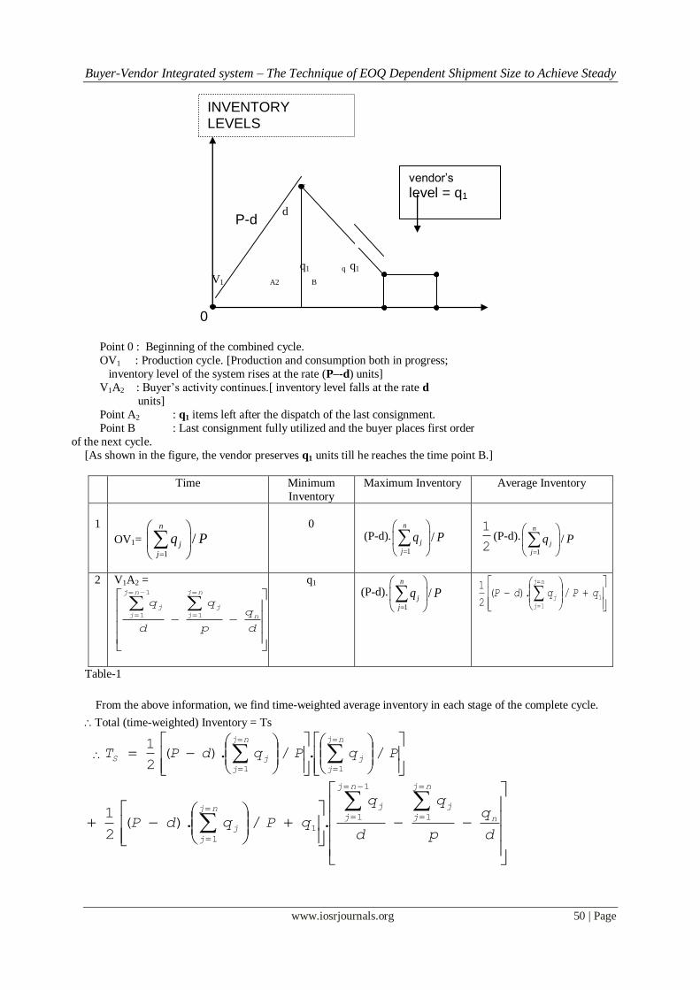
The following figure clarifies the complete behavior of the system.



d

q1 q q1

V1 A2 B

Point 0 : Beginning of the combined cycle.

OV1 : Production cycle. [Production and consumption both in progress;

inventory level of the system rises at the rate (P–-d) units]

V1A2 : Buyer‘s activity continues.[ inventory level falls at the rate d

units]

Point A2 : q1 items left after the dispatch of the last consignment.

Point B : Last consignment fully utilized and the buyer places first order

of the next cycle.

[As shown in the figure, the vendor preserves q1 units till he reaches the time point B.]

Time Minimum

Inventory

Maximum Inventory Average Inventory

1

OV1=

1

/n

j

j

q P

0

(P-d).

1

/n

j

j

q P

1

2(P-d).

1

/n

j

j

q P

2 V1A2 =

d

q

p

q

d

q

n

nj

j

j

nj

j

j

1

1

1

q1

(P-d).

1

/n

j

j

q P

1

1

/).(2

1qPqdP

nj

j

j

Table-1

From the above information, we find time-weighted average inventory in each stage of the complete cycle.

Total (time-weighted) Inventory = Ts

PqPqdPT

nj

j

j

nj

j

jS/./).(

2

1

11

d

q

p

q

d

q

qPqdP n

nj

j

j

nj

j

jnj

j

j

1

1

1

1

1

./).(2

1

P-d

2V

2V

2V

2V

0

2V

2V

2V

vendor’s

level = q1

INVENTORY LEVELS



=

PqPqdP

nj

j

j

nj

j

j//).(

2

1

11

d

q

pdqqPqdP n

nj

j

j

nj

j

j

11/).(

2

1

1

1

1

Simplifying this expression we get,

TS =

1 1

1

1

.2.

2

j n

j j nj n

j n

j

p d qq q

q q qpd d

We divide this expression by

q

d

j

j

j n

1

to get average inventory of the

system per unit time.

qS =

1

1

1

1

.2.

2

j n

nj n j n

j

j

j

p d q qq q q

pq

(7)

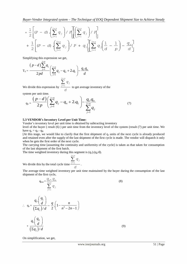
5.3 VENDOR’s Inventory Level per Unit Time:

Vendor‘s inventory level per unit time is obtained by subtracting inventory

level of the buyer ( result (6) ) per unit time from the inventory level of the system (result (7) per unit time. We

have qv = qS - qB

[At this stage, we would like to clarify that the first shipment of q1 units of the next cycle is already produced

and retained even after the supply of the last shipment of the first cycle is made. The vendor will dispatch it only when he gets the first order of the next cycle.

The carrying time [assuming the continuity and uniformity of the cycle] is taken as that taken for consumption

of the last shipment of the first batch.

The time weighted inventory during this segment is (q1).(qn/d).

We divide this by the total cycle time

q

d

j

j

j n

1

.

The average time weighted inventory per unit time maintained by the buyer during the consumption of the last

shipment of the first cycle,

qlast =q q

q

n

j

j

j n

1

1

.

(8)

qv =

11.

/j

qq

d

q d

--

3. 1

2 2 1

q n

n n

+

1

/

n

j

qq

d

q d

(9)

On simplification, we get,



qv =

1

1

. 2.2

j n

j n

j

p dq q q

p

--

3. 1

2 2 1

q n

n n

(10)

V. Structure of the Cost Function and Optimization: Using the above facts, we construct cost function TIC(q, n).

It is composed of three parts.

1 Set-up Cost

2 Ordering Cost

1 Carrying Cost (of Buyer and Vendor)

BV

jj

qhqhq

dAn

q

PAnqTIC

2131..,

.

(11)

Where q q nn

n .( / )1 1 , 1

1. 1q q

n

1

12

1

n

nnqq

nj

j

j = 1

.1

q nn

qv =

1

1

. 2.2

j n

j n

j

p dq q q

p

--

3. 1

2 2 1

q n

n n

qB = 3

. 12 2 1

q n

n n

In order to simplify and extend the calculations, we introduce the following notations.

k1 = A1P+nA3d k2 = (P-d) /2P k3 = 1

1n

n

k4 = 1

1nn

k5 = (1 – 1/n) k6 =

31

2 1

n

n n

Introducing these notations in the above equation (11), we write

2

11 2 3 4 5 6 1

3

, . . 2 .. 2

k qTIC q n h k k k k k h h

q k .. (12)

We differentiate (12) partially w.r.to q treating ‗n‘ as an integer constant. (We have considered n>3, an integer).

( , )TIC q n

q

11 2 3 4 5 6 2 12

3

1 1. . . 2 .

2

kh k k k k k h h

k q

. . (13)

Also, 2

1

2 3

3

, 2 1.

TIC q n k

q k q

> 0 .(14)



It ensures minimization of TICq n( , ) at q = q* obtained by equating the result

(13) with zero. This, in turn, gives

q q *=

1

1/ 2

1

3 1 2 3 4 5 6 2 1

2

. . 2

k

k h k k k k k h h

(15)

This value of q q * gives basic quantity which is useful to derive the size of shipment in each quantity.(for

a fixed value of n—number of shipments; n 3.)

TIC q n( , )*

= 1

1/ 2

1 3 1 2 3 4 5 6 2 12 . . 2k k h k k k k k h h (16)

All Ki, i = 1 to 6.are pre-defined as above.

Note:

1. In the above results (15) and (16), All Ki, i = 1 to 6 are constants depending on given situation (data) and

n>3, is a fixed integer.

2. We have already assumed that h1 < h2; as inventory items stream down from manufacturer to buyers, the

holding cost increases.

Even if both are equal then

E.O.Q.= q q *=

1/ 2

1

3 1 2 3 4 5

2

. . . 2

k

k h k k k k

(17)

And,

TIC q n( , )*

= 1/ 2

1 3 1 2 3 4 52. . . . 2k k h k k k k (18)

VI. Some Related Deductions: 7.1 Shipment and quantity pattern: As we know, qj = q (1 – 1/nj ) with j = 1, 2, 3, 4……. and n>3

For a fixed n, we have, for q = q*

Shipment Quantity

1 q1 = q* (1 - 1/n)

2 q2 = q* (1 - 1/n2)

3 q3 = q* (1 - 1/n3)

, ………………………..

. …………………………

i qi = q* (1 - 1/ni)

This implies that

n

i

jjn

nqq1

* 1

and

n

n

nn

nn

j

j11

1111

1

1

11

n

n

n

for large values of n. 1

0nn

Comment:

This clearly implies that after three or four shipments the remaining shipments



are integrally of the same size. This is what we wanted to achieve - stability in the shipment size.

This gives qj

= * 1

1q n

n

qj

= q*.k3 (19)

7.2 Cycle Times: In one complete cycle of the system,

Vendor‘s Production Time Pqj/

Using above formula,

Vendor‘s Production Time P

kq3

.

….(20)

Buyer‘s active participation =

2

1

/j

j

j

q d

q k

d

*.

3 ….(21)

From the above results, we find the time-slot for which the production process remains busy for another buyer

with the demand of the same type of units or changes the set-up in favor of some new buyer with different

pattern, is given by the following result.

This time period is Pd

qj

11.

We denote this by the notation TF.

TF =

Pd

dPq

j. =

d

kkq

.2

..32

*

(22)

7.3 Review Period: This is the time-slot, a part of one complete cycle, during which both the buyer and vendor can review the

discrepancies and issues observed during the execution of the operation. This time-period is between the

dispatch of the last shipment and placement of the first order of the next cycle.

The nth shipment is scheduled on complete consumption of (n-1) shipment.

Time to consume nth shipment is,.

Denoting the review period by the notation Tr we have:

Tr = dnqd

q nn /)/11.(*

Ignoring nn

1 as 1/nn 0,

Tr =

2

1

/j

j

j

q d

….(23)

7.4 Incremental Production: It is defined as the number of units that the system can produce after completion of its total production of the

first buyer. The vendor gets the free time (defined in last section of (7.2) = TF

Production during this period = P.TF = P.dk

kq

3

2

*

.2

. ….(24)



8. Illustration:

We clarify our views by the following example.

Vendor‘s facts Buyer‘s facts

(1) P = 3200 units (1) d = 1000 units

(2) A1 = 400 (2) h2 = 5

(3) A3 = 25

(4) h1 = 4 We take n = 5, 6, 7, 8 etc.

We find q*(EOQ), TIC(q*, n)--Total incremental cost--, qj, and cycle length Finally we plot graphs of ‗n‘ and corresponding TIC(q*, n)

We calculate K1, K2, K3, etc. using the following relations (already defined in earlier section.) Necessary results

and formulae are given below.

k1 = A1P+nA3d k2 = (P-d) /2P k3 = 1

1n

n

k4 = 1

1nn

k5 = (1 – 1/n) k6 =

31

2 1

n

n n

EOQ = q* =

1

1/ 2

1

3 1 2 3 4 5 6 2 1

2

. . 2

k

k h k k k k k h h

TIC q n( , )*

= 1

1/ 2

1 3 1 2 3 4 5 6 2 12 . . 2k k h k k k k k h h

The following table shows EOQ thw case of n = 3,4,5,6 number of shipments. It is seen that after two or three

shipments each less than the size of EOQ; the shipment size tends to consistency.

Shipment size

n EOQ Q1 Q2 Q3 Q4 Q5 Q6 Q7

3 475 352 422 457 -- --- --- --

4 336 252 315 331 335 ---- --- --

5 234 187 225 232 234 234 --- --

6 224 187 218 223 224 224 224 --

7 224 219 223 224 224 224 224 224

Table-2

Total Shipment and Unit incremental cost

Number of

shipments

EOQ Total units of

shipment

TIC Unit Cost

3 475 1196 5701 4.77

4 336 1232 8211 6.66

5 234 1112 9257 8.32

6 224 1300 12750 9.84

7 194 1530 15028 9.82

Table-3

It can be seen that as the number of shipments increases; the shipment size tends to attain consistency.



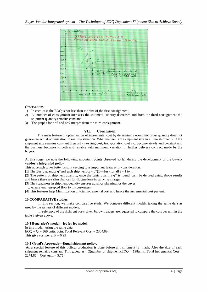
Observations:

1) In each case the EOQ is not less than the size of the first consignment.

2) As number of consignment increases the shipment quantity decreases and from the third consignment the

shipment quantity remains constant.

3) The graphs for n=6 and n=7 merges from the third consignment.

VII. Conclusion: The main feature of optimization of incremental cost by determining economic order quantity does not

guarantee actual optimization in real life situation. What matters is the shipment size in all the shipments. If the

shipment size remains constant then only carrying cost, transportation cost etc. become steady and constant and

the business becomes smooth and reliable with minimum variation in further delivery contract made by the

buyers.

At this stage, we note the following important points observed so far during the development of the buyer-

vendor’s integrated policy

This approach gives better results keeping four important features in consideration.

[1] The Basic quantity q*and each shipment qj = q*(1—1/nj) for all j = 1 to n.

[2] The pattern of shipment quantity, once the basic quantity q* is found, can be derived using above results

and hence there are slim chances for fluctuations in carrying charges.

[3] The steadiness in shipment quantity ensures advance planning for the buyer to ensure uninterrupted flow to his customers.

[4] This features help Minimization of total incremental cost and hence the incremental cost per unit.

10 COMPARATIVE studies: In this section, we make comparative study. We compare different models taking the same data as

used by the writers of different models.

In reference of the different costs given below, readers are requested to compare the cost per unit in the

table 3 given above.

10.1 Benerajee’s model—lot for lot model. In this model, using the same data, EOQ = Q*= 369 units, Joint Total Relevant Cost = 2304.89

This give cost per unit = 6.25

10.2 Goyal’s Approach—Equal shipment policy.

As a special feature of this policy, production is done before any shipment is made. Also the size of each

shipment remains constant. This gives; n = 2(number of shipment),EOQ = 198units. Total Incremental Cost =

2274.86 Cost /unit = 5.75



10.3 Goyal’s approach—Increasing (At a constant rate) size of shipment.

First Lot = Q*= 36 units incremental factor = 3.2 (= P/D), n = 3

Shipment 1 – size 36 units, Shipment 2—size 116 units, Shipment 3—Size 371

units. Total incremental cost = 1818

cost / unit = 3.48

(The variation in the size of shipments may not be acceptable in reality. The third shipment is more than ten

times in size than that of the first one. This very unrealistic situations is liable to affect the carrying charges which practically

changes or depends not on a linear rule.

10.4 Roger Hill’s approach—increasing size of shipment.

The cost function has three variables— q, n, and ; q — the size of first lot. [For a fixed value of n, q* is derived and it becomes the first shipment in a sequence of n shipments. As against this, the plans suggested in

this paper, determines the basic quantity q* which in turn is used to derive the size of each one of n shipments],

the incremental factor = (1 P/D), and n= number of shipments.

Extending the plans of Dr.Roger Hills, we derive that = 1.16 and for n=8 shipments, the size of the first shipment= q* = 41 items.

According to his recommended pattern, for the value of (approximated using algorithm),the shipments quantity in eight shipments shall be 41,48,55,64,74,86,100 and 118 units in order, which adds up to 584 items in

total.

This finally gives $ 3.5 as incremental cost/unit

Also it reflects that eighth shipment size is nearly three times that of the first one.!!

We, just by concentrating upon the number of shipments and the size of each shipment having high fluctuations in consecutive shipments(which is liable to fluctuations in carrying charges), have recommended the steady plan

and steady flow that ensures both the constant flow of items to the buyer, uniformity in carrying charges, and

minimal joint incremental cost and hence steady and pre-planned business.

References: [1]. Benerjee, A, (1986) ,‘ A joint economic lot size model for purchaser and vendor ‗, Decision Science 17,292. 311

[2]. Goyal. S. K (1977),‘Determination of optimum production quantity for a two- stage production system‖ , Operational Research

Quartely 28, 865-870

[3]. Goyal. S. K. (1988) ,‖ A joint economic lot size model for purchaser and vendor; A comment , Decision Sciences 19,236-241

[4]. Goyal S. K.( 1995), ― a one – vendor multi-buyer integrated inventory Model‖ . A Comment‖ European Journal if Operations Research

82, 209- 210

[5]. Lu. L (1995) ― A one vendor multi buyer integrated inventory Models‖ European Journal of Operations Research.

[6]. Jha.Pradeep.j ( 2009) , ― Buyer Vendor Integrated System( time Scaling and Normalization), Ph.D. Thesis to North _Gujarat

University, 5, 56-75