Embed Size (px)
Citation preview
Analysis of Branch Misses in Quicksort
Sebastian [email protected]
based on joint work with Conrado Martínez and Markus E. Nebel
04 January 2015
Meeting on Analytic Algorithmics and Combinatorics
Sebastian Wild Branch Misses in Quicksort 2015-01-04 1 / 15

Instruction Pipelines
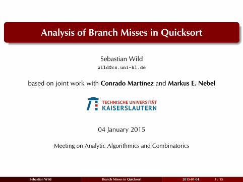
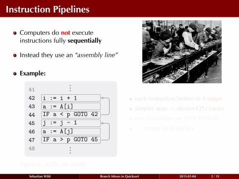
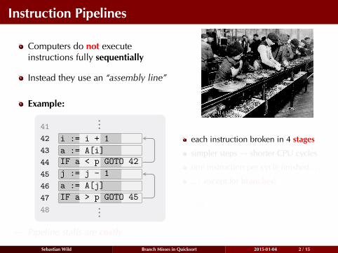
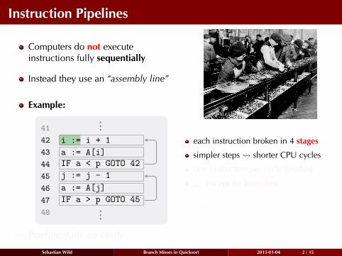
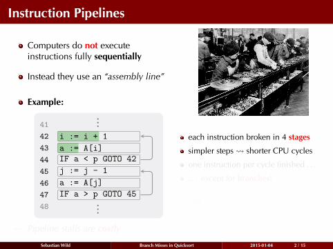
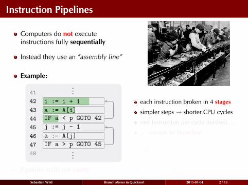
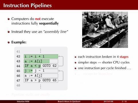
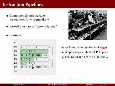
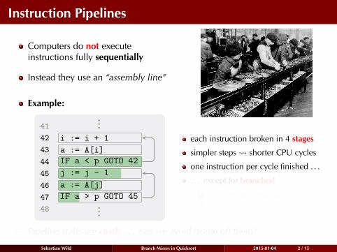
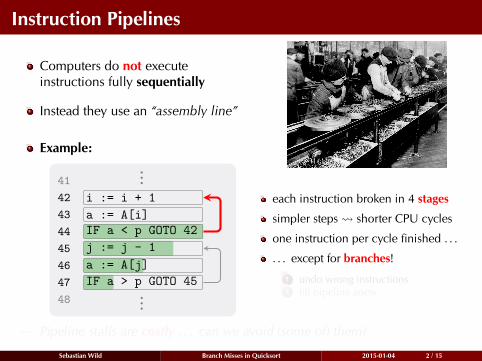
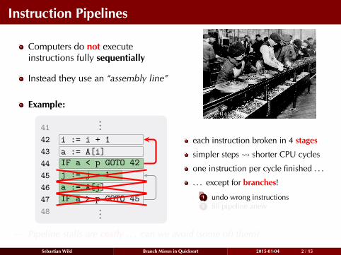
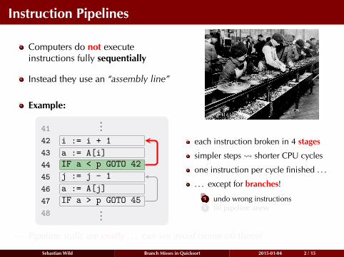
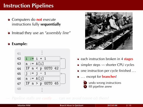
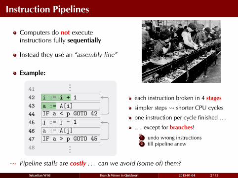
Computers do not executeinstructions fully sequentially
Instead they use an “assembly line”
Example:
424344454647
41
48
...i := i + 1a := A[i]IF a < p GOTO 42j := j - 1a := A[j]IF a > p GOTO 45
...
each instruction broken in 4 stages
simpler steps shorter CPU cycles
one instruction per cycle finished . . .
. . . except for branches!
1 undo wrong instructions2 fill pipeline anew
Pipeline stalls are costly . . . can we avoid (some of) them?
Sebastian Wild Branch Misses in Quicksort 2015-01-04 2 / 15
Instruction Pipelines
Computers do not executeinstructions fully sequentially
Instead they use an “assembly line”
Example:
424344454647
41
48
...i := i + 1a := A[i]IF a < p GOTO 42j := j - 1a := A[j]IF a > p GOTO 45
...
each instruction broken in 4 stages
simpler steps shorter CPU cycles
one instruction per cycle finished . . .
. . . except for branches!
1 undo wrong instructions2 fill pipeline anew
Pipeline stalls are costly . . . can we avoid (some of) them?
Sebastian Wild Branch Misses in Quicksort 2015-01-04 2 / 15
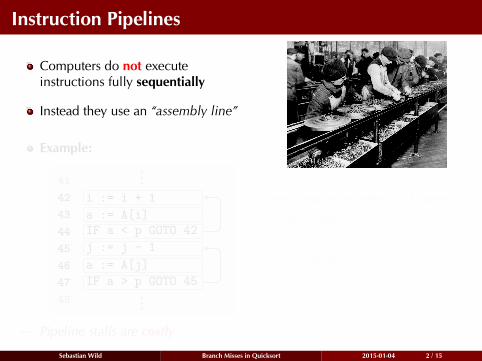
Branch Prediction
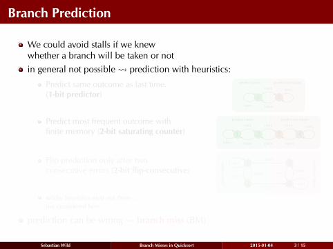
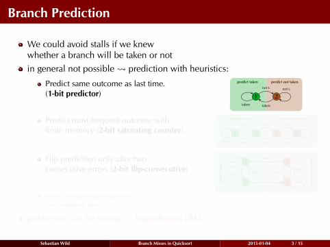
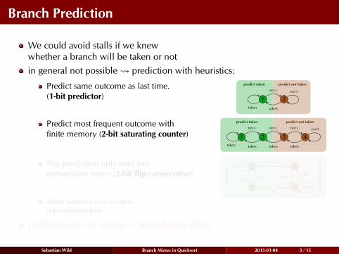
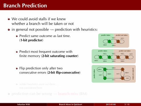
We could avoid stalls if we knewwhether a branch will be taken or notin general not possible prediction with heuristics:
Predict same outcome as last time.(1-bit predictor) 1 2
predict taken predict not taken
taken
not t. not t.
taken
Predict most frequent outcome withfinite memory (2-bit saturating counter) 1 2 3 4
predict taken predict not taken
taken
not t. not t. not t. not t.
takentakentaken
Flip prediction only after twoconsecutive errors (2-bit flip-consecutive)
pred
ictt
aken
predictnottaken
1
2
3
4
taken
not t.taken
not t.not t.
takennot t.
taken
wilder heuristics exist out there . . .not considered here
prediction can be wrong branch miss (BM)
Sebastian Wild Branch Misses in Quicksort 2015-01-04 3 / 15
Branch Prediction
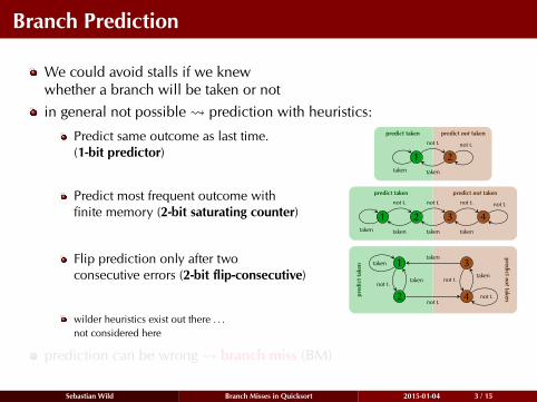
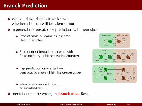
We could avoid stalls if we knewwhether a branch will be taken or notin general not possible prediction with heuristics:
Predict same outcome as last time.(1-bit predictor) 1 2
predict taken predict not taken
taken
not t. not t.
taken
Predict most frequent outcome withfinite memory (2-bit saturating counter) 1 2 3 4
predict taken predict not taken
taken
not t. not t. not t. not t.
takentakentaken
Flip prediction only after twoconsecutive errors (2-bit flip-consecutive)
pred
ictt
aken
predictnottaken
1
2
3
4
taken
not t.taken
not t.not t.
takennot t.
taken
wilder heuristics exist out there . . .not considered here
prediction can be wrong branch miss (BM)
Sebastian Wild Branch Misses in Quicksort 2015-01-04 3 / 15

Why Should We Care?
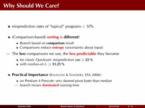
misprediction rates of “typical” programs < 10%
(Comparison-based) sorting is different!Branch based on comparison resultComparisons reduce entropy (uncertainty about input)
The less comparisons we use, the less predictable they becomefor classic Quicksort: misprediction rate > 25 %with median-of-3: > 31.25 %
Practical Importance (KALIGOSI & SANDERS, ESA 2006):
on Pentium 4 Prescott: very skewed pivot faster than median branch misses dominated running time
Sebastian Wild Branch Misses in Quicksort 2015-01-04 4 / 15

Why Should We Care?
misprediction rates of “typical” programs < 10%
(Comparison-based) sorting is different!Branch based on comparison resultComparisons reduce entropy (uncertainty about input)
The less comparisons we use, the less predictable they becomefor classic Quicksort: misprediction rate > 25 %with median-of-3: > 31.25 %
Practical Importance (KALIGOSI & SANDERS, ESA 2006):
on Pentium 4 Prescott: very skewed pivot faster than median branch misses dominated running time
Sebastian Wild Branch Misses in Quicksort 2015-01-04 4 / 15
Track Record of Dual-Pivot Quicksort
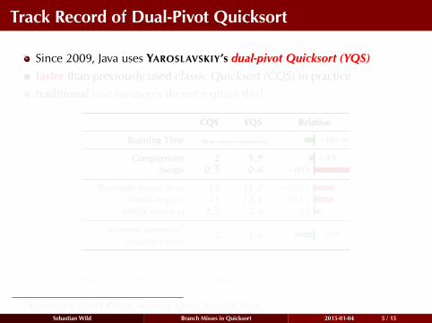
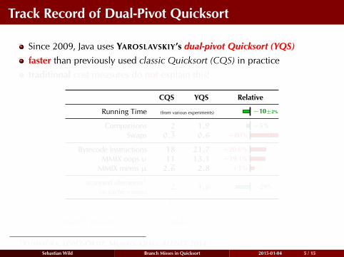
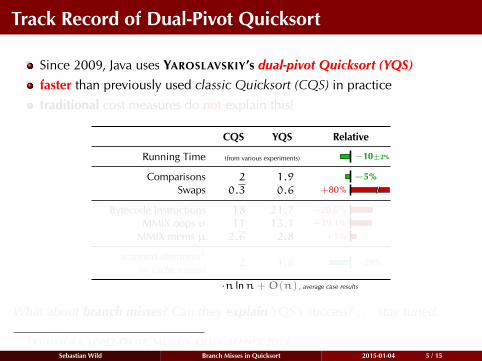
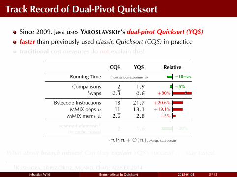
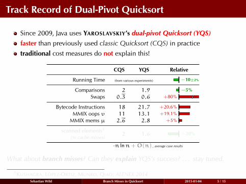
Since 2009, Java uses YAROSLAVSKIY’s dual-pivot Quicksort (YQS)faster than previously used classic Quicksort (CQS) in practicetraditional cost measures do not explain this!
CQS YQS Relative
Running Time (from various experiments) −10±2%
Comparisons 2 1.9 −5%Swaps 0.3 0.6 +80%
Bytecode Instructions 18 21.7 +20.6%MMIX oops υ 11 13.1 +19.1%
MMIX mems µ 2.6 2.8 +5%
scanned elements1
(≈ cache misses)2 1.6 −20%
·n lnn+O(n) , average case results
What about branch misses? Can they explain YQS’s success? . . . stay tuned.
1KUSHAGRA, LÓPEZ-ORTIZ, MUNRO, QIAO; ALENEX 2014Sebastian Wild Branch Misses in Quicksort 2015-01-04 5 / 15
Track Record of Dual-Pivot Quicksort
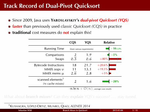
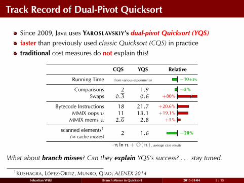
Since 2009, Java uses YAROSLAVSKIY’s dual-pivot Quicksort (YQS)faster than previously used classic Quicksort (CQS) in practicetraditional cost measures do not explain this!
CQS YQS Relative
Running Time (from various experiments) −10±2%
Comparisons 2 1.9 −5%Swaps 0.3 0.6 +80%
Bytecode Instructions 18 21.7 +20.6%MMIX oops υ 11 13.1 +19.1%
MMIX mems µ 2.6 2.8 +5%
scanned elements1
(≈ cache misses)2 1.6 −20%
·n lnn+O(n) , average case results
What about branch misses? Can they explain YQS’s success? . . . stay tuned.
1KUSHAGRA, LÓPEZ-ORTIZ, MUNRO, QIAO; ALENEX 2014Sebastian Wild Branch Misses in Quicksort 2015-01-04 5 / 15
Random Model
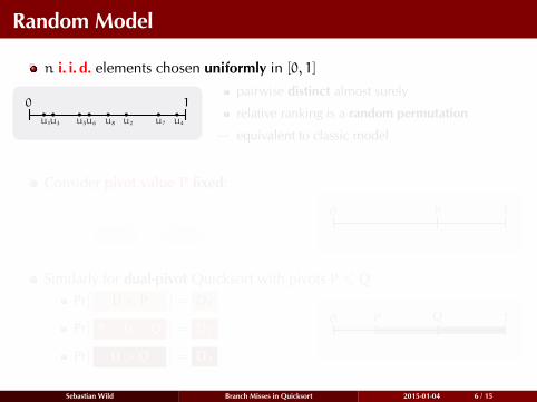
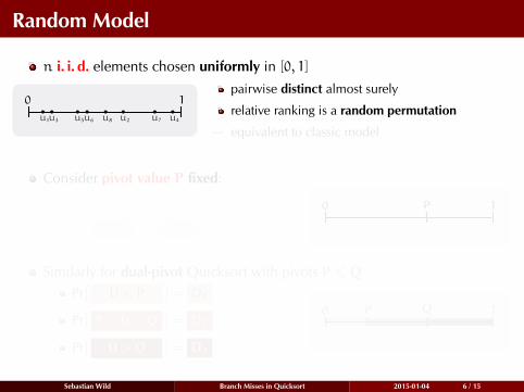
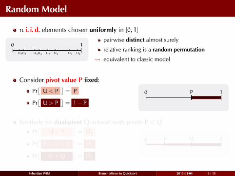
n i. i. d. elements chosen uniformly in [0, 1]
0 1
U1 U2U3 U4U5U6 U7U8
pairwise distinct almost surely
relative ranking is a random permutation
equivalent to classic model
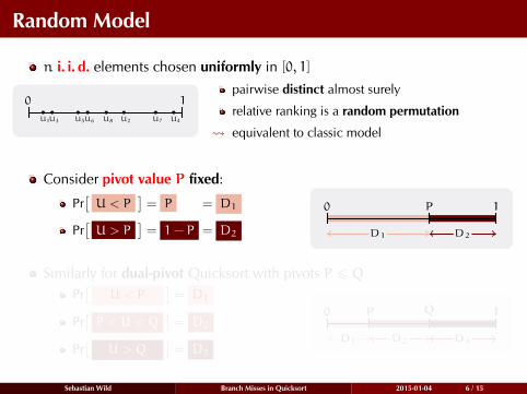
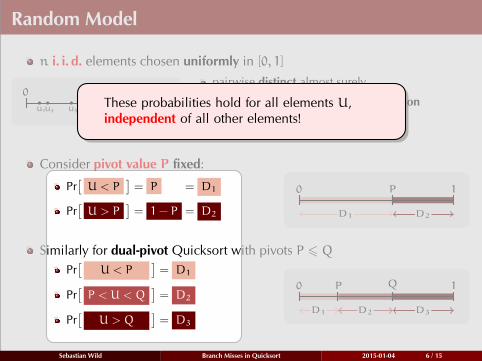
Consider pivot value P fixed:
Pr[U < P
]= P
= D1
Pr[U > P
]= 1− P
= D2
0 1P
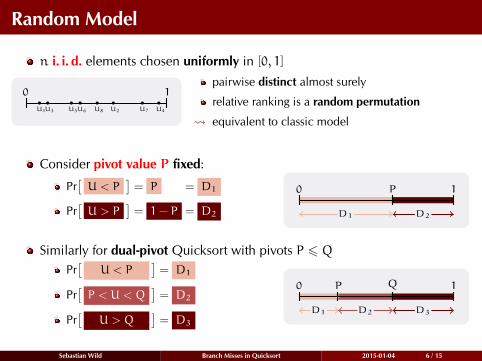
Similarly for dual-pivot Quicksort with pivots P 6 QPr[
U < P]= D1
Pr[P < U < Q
]= D2
Pr[
U > Q]= D3
0 1P Q
These probabilities hold for all elements U,independent of all other elements!
Sebastian Wild Branch Misses in Quicksort 2015-01-04 6 / 15
Random Model
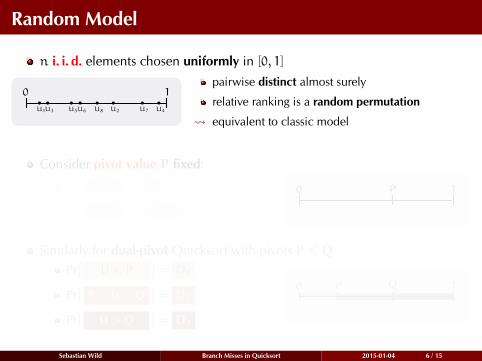
n i. i. d. elements chosen uniformly in [0, 1]
0 1
U1 U2U3 U4U5U6 U7U8
pairwise distinct almost surely
relative ranking is a random permutation
equivalent to classic model
Consider pivot value P fixed:
Pr[U < P
]= P
= D1
Pr[U > P
]= 1− P
= D2
0 1P
Similarly for dual-pivot Quicksort with pivots P 6 QPr[
U < P]= D1
Pr[P < U < Q
]= D2
Pr[
U > Q]= D3
0 1P Q
These probabilities hold for all elements U,independent of all other elements!
Sebastian Wild Branch Misses in Quicksort 2015-01-04 6 / 15
Random Model
n i. i. d. elements chosen uniformly in [0, 1]
0 1
U1 U2U3 U4U5U6 U7U8
pairwise distinct almost surely
relative ranking is a random permutation
equivalent to classic model
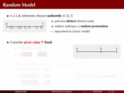
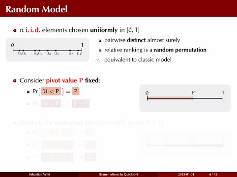
Consider pivot value P fixed:
Pr[U < P
]= P = D1
Pr[U > P
]= 1− P = D2
0 1P
D1 D2
Similarly for dual-pivot Quicksort with pivots P 6 QPr[
U < P]= D1
Pr[P < U < Q
]= D2
Pr[
U > Q]= D3
0 1P Q
D1 D2 D3
These probabilities hold for all elements U,independent of all other elements!
Sebastian Wild Branch Misses in Quicksort 2015-01-04 6 / 15
Random Model
n i. i. d. elements chosen uniformly in [0, 1]
0 1
U1 U2U3 U4U5U6 U7U8
pairwise distinct almost surely
relative ranking is a random permutation
equivalent to classic model
Consider pivot value P fixed:
Pr[U < P
]= P = D1
Pr[U > P
]= 1− P = D2
0 1P
D1 D2
Similarly for dual-pivot Quicksort with pivots P 6 QPr[
U < P]= D1
Pr[P < U < Q
]= D2
Pr[
U > Q]= D3
0 1P Q
D1 D2 D3
These probabilities hold for all elements U,independent of all other elements!
Sebastian Wild Branch Misses in Quicksort 2015-01-04 6 / 15

Branches in CQS
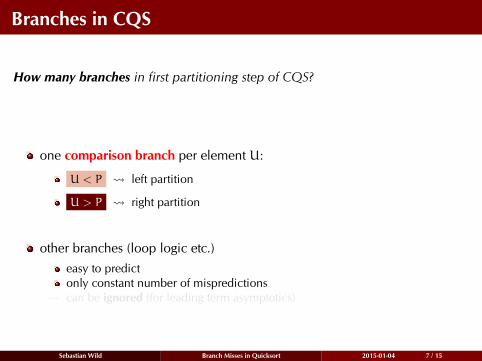
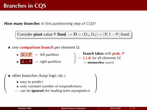
How many branches in first partitioning step of CQS?
Consider pivot value P fixed. D = (D1, D2) = (P, 1− P) fixed.
one comparison branch per element U:
U < P left partition
U > P right partition
}
branch taken with prob. Pi. i. d. for all elements U! memoryless source
other branches (loop logic etc.)easy to predictonly constant number of mispredictions
can be ignored (for leading term asymptotics)
Sebastian Wild Branch Misses in Quicksort 2015-01-04 7 / 15

Branches in CQS
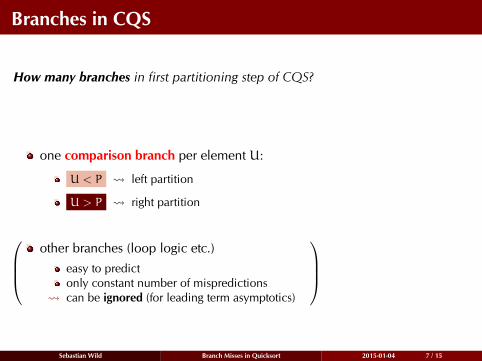
How many branches in first partitioning step of CQS?
Consider pivot value P fixed. D = (D1, D2) = (P, 1− P) fixed.
one comparison branch per element U:
U < P left partition
U > P right partition
}
branch taken with prob. Pi. i. d. for all elements U! memoryless source
other branches (loop logic etc.)easy to predictonly constant number of mispredictions
can be ignored (for leading term asymptotics)
Sebastian Wild Branch Misses in Quicksort 2015-01-04 7 / 15
Branches in CQS
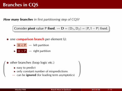
How many branches in first partitioning step of CQS?
Consider pivot value P fixed. D = (D1, D2) = (P, 1− P) fixed.
one comparison branch per element U:
U < P left partition
U > P right partition
}
branch taken with prob. Pi. i. d. for all elements U! memoryless source
other branches (loop logic etc.)easy to predictonly constant number of mispredictions
can be ignored (for leading term asymptotics)
Sebastian Wild Branch Misses in Quicksort 2015-01-04 7 / 15
Branches in CQS
How many branches in first partitioning step of CQS?
Consider pivot value P fixed. D = (D1, D2) = (P, 1− P) fixed.
one comparison branch per element U:
U < P left partition
U > P right partition
}
branch taken with prob. Pi. i. d. for all elements U! memoryless source
other branches (loop logic etc.)
easy to predictonly constant number of mispredictions
can be ignored (for leading term asymptotics)
Sebastian Wild Branch Misses in Quicksort 2015-01-04 7 / 15
Branches in CQS
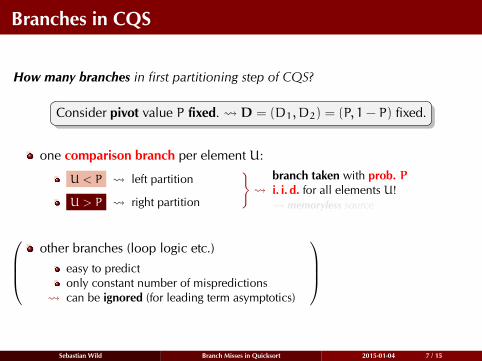
How many branches in first partitioning step of CQS?
Consider pivot value P fixed. D = (D1, D2) = (P, 1− P) fixed.
one comparison branch per element U:
U < P left partition
U > P right partition
}
branch taken with prob. Pi. i. d. for all elements U! memoryless source
other branches (loop logic etc.)
easy to predictonly constant number of mispredictions
can be ignored (for leading term asymptotics)
Sebastian Wild Branch Misses in Quicksort 2015-01-04 7 / 15
Misprediction Rate for Memoryless Sources
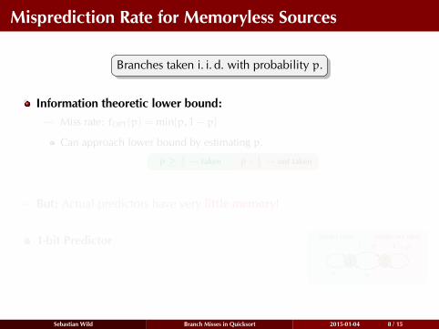
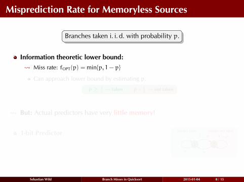
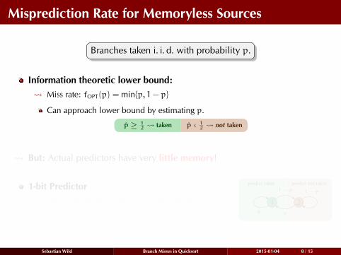
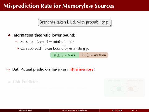
Branches taken i. i. d. with probability p.
Information theoretic lower bound: Miss rate: fOPT(p) = min{p, 1− p}
Can approach lower bound by estimating p.
p̂ ≥ 12 taken p̂ < 1
2 not taken
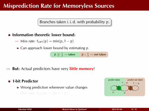
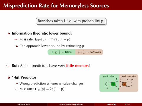
But: Actual predictors have very little memory!
1-bit PredictorWrong prediction whenever value changes
Miss rate: f1bit(p) = 2p(1− p)
1 2
predict taken predict not taken
p
1−p 1−p
p
Sebastian Wild Branch Misses in Quicksort 2015-01-04 8 / 15
Misprediction Rate for Memoryless Sources
Branches taken i. i. d. with probability p.
Information theoretic lower bound: Miss rate: fOPT(p) = min{p, 1− p}
Can approach lower bound by estimating p.
p̂ ≥ 12 taken p̂ < 1
2 not taken
But: Actual predictors have very little memory!
1-bit PredictorWrong prediction whenever value changes
Miss rate: f1bit(p) = 2p(1− p)
1 2
predict taken predict not taken
p
1−p 1−p
p
Sebastian Wild Branch Misses in Quicksort 2015-01-04 8 / 15
Misprediction Rate for Memoryless Sources [2]
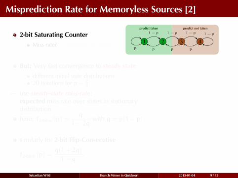
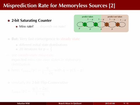
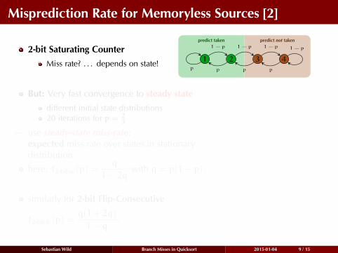
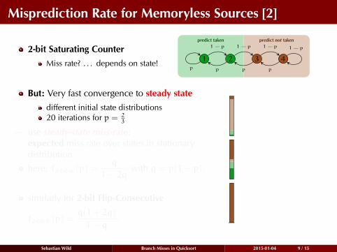
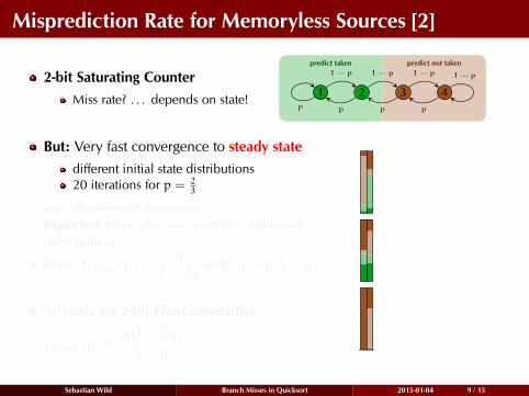
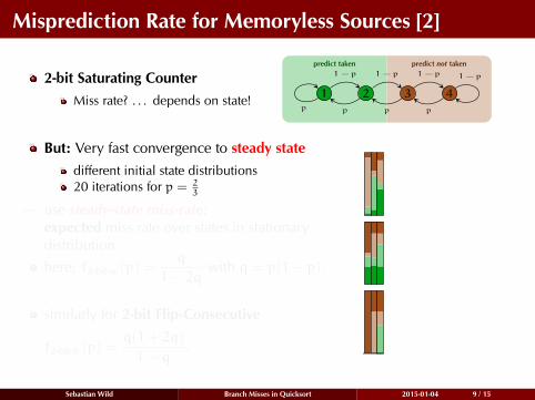
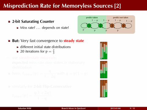
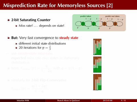
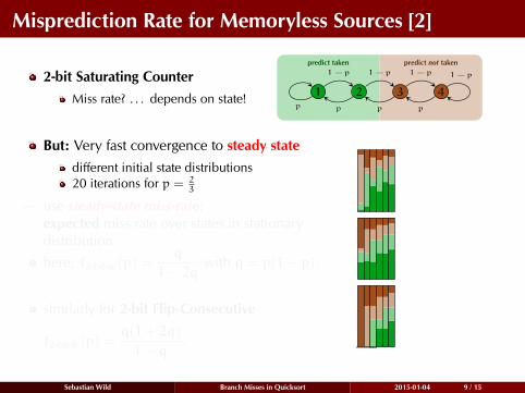
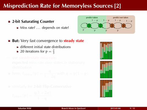
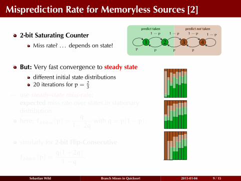
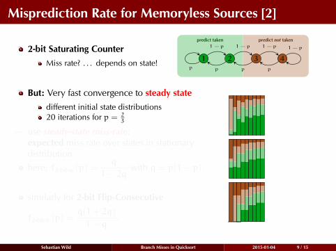
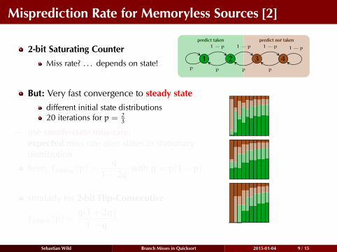
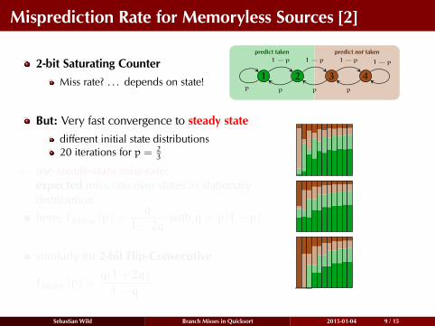
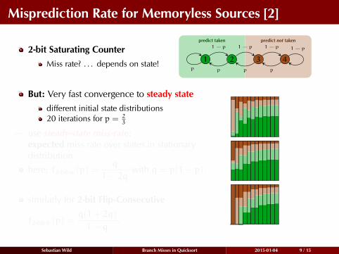
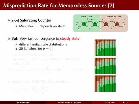
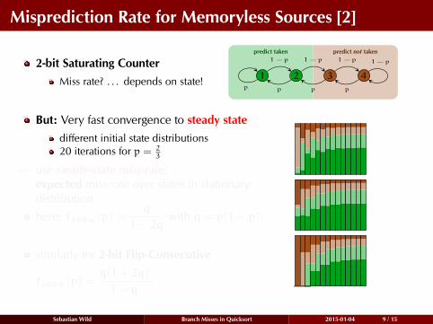
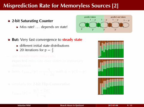
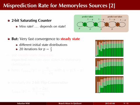
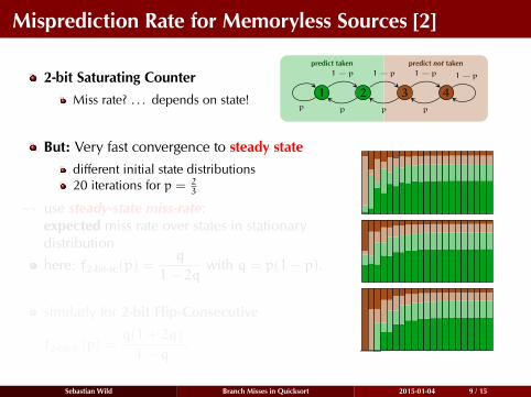
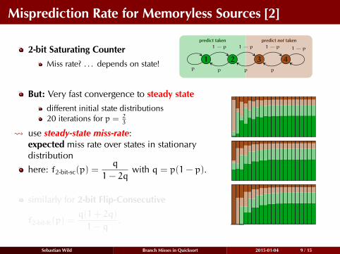
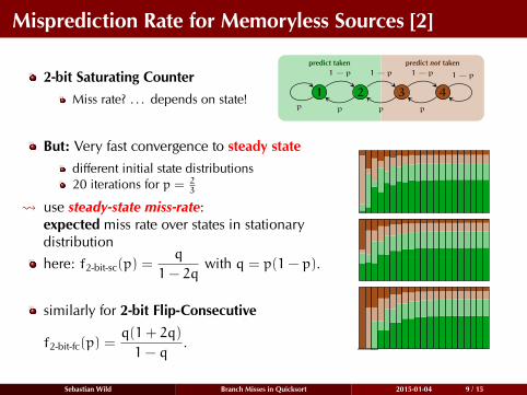
2-bit Saturating CounterMiss rate? . . . depends on state! 1 2 3 4
predict taken predict not taken
p
1−p 1−p 1−p 1−p
ppp
But: Very fast convergence to steady statedifferent initial state distributions20 iterations for p = 2
3
use steady-state miss-rate:expected miss rate over states in stationarydistributionhere: f2-bit-sc(p) =
q
1− 2qwith q = p(1− p).
similarly for 2-bit Flip-Consecutive
f2-bit-fc(p) =q(1+ 2q)
1− q.
Sebastian Wild Branch Misses in Quicksort 2015-01-04 9 / 15
Misprediction Rate for Memoryless Sources [2]
2-bit Saturating CounterMiss rate? . . . depends on state! 1 2 3 4
predict taken predict not taken
p
1−p 1−p 1−p 1−p
ppp
But: Very fast convergence to steady statedifferent initial state distributions20 iterations for p = 2
3
use steady-state miss-rate:expected miss rate over states in stationarydistributionhere: f2-bit-sc(p) =
q
1− 2qwith q = p(1− p).
similarly for 2-bit Flip-Consecutive
f2-bit-fc(p) =q(1+ 2q)
1− q.
Sebastian Wild Branch Misses in Quicksort 2015-01-04 9 / 15
Distribution of Pivot Values
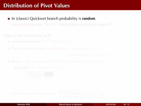
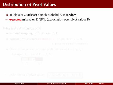
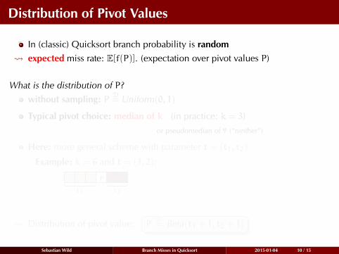
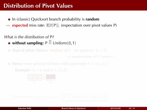
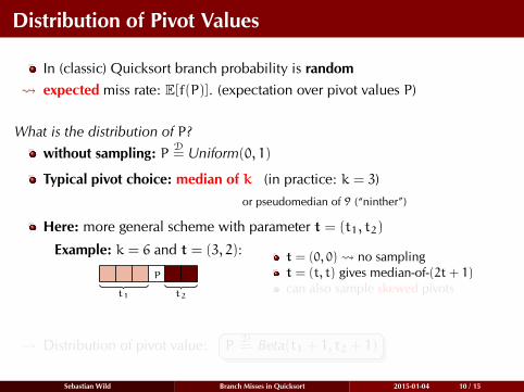
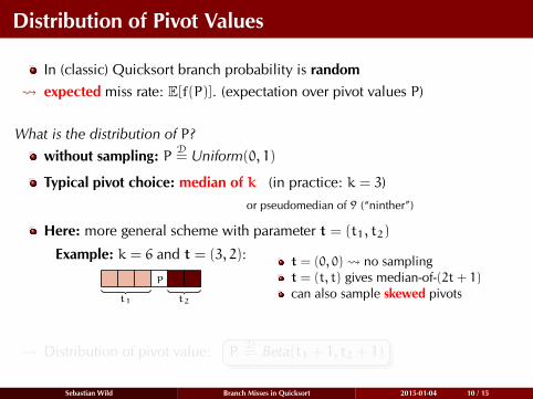
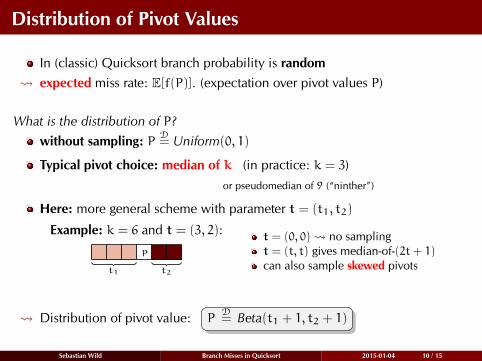
In (classic) Quicksort branch probability is random expected miss rate: E[f(P)]. (expectation over pivot values P)
What is the distribution of P?without sampling: P D
= Uniform(0, 1)
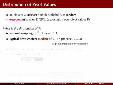
Typical pivot choice: median of k (in practice: k = 3)or pseudomedian of 9 (“ninther”)
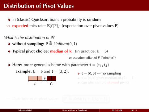
Here: more general scheme with parameter t = (t1, t2)
Example: k = 6 and t = (3, 2):
P
t1 t2
t = (0, 0) no samplingt = (t, t) gives median-of-(2t+ 1)can also sample skewed pivots
Distribution of pivot value: PD= Beta(t1 + 1, t2 + 1)
Sebastian Wild Branch Misses in Quicksort 2015-01-04 10 / 15
Distribution of Pivot Values
In (classic) Quicksort branch probability is random expected miss rate: E[f(P)]. (expectation over pivot values P)
What is the distribution of P?without sampling: P D
= Uniform(0, 1)
Typical pivot choice: median of k (in practice: k = 3)or pseudomedian of 9 (“ninther”)
Here: more general scheme with parameter t = (t1, t2)
Example: k = 6 and t = (3, 2):
P
t1 t2
t = (0, 0) no samplingt = (t, t) gives median-of-(2t+ 1)can also sample skewed pivots
Distribution of pivot value: PD= Beta(t1 + 1, t2 + 1)
Sebastian Wild Branch Misses in Quicksort 2015-01-04 10 / 15
Miss Rates for Quicksort Branch
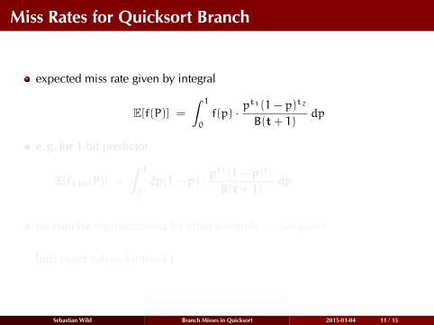
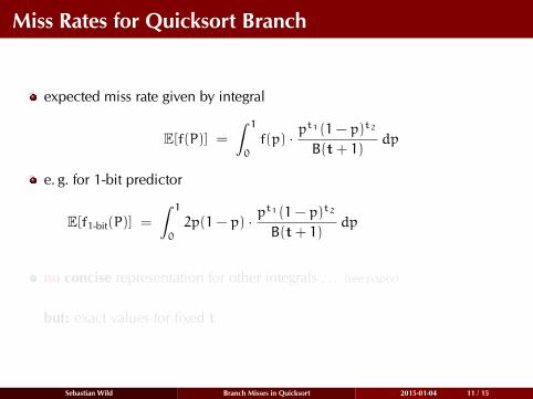
expected miss rate given by integral
E[f(P)] =
ˆ 10
f(p) · pt1(1− p)t2
B(t+ 1)dp
e. g. for 1-bit predictor
E[f1-bit(P)] =
ˆ 10
2p(1− p) · pt1(1− p)t2
B(t+ 1)dp
= 2(t1 + 1)(t2 + 1)
(k+ 2)(k+ 1)
no concise representation for other integrals . . . (see paper)
but: exact values for fixed t
Sebastian Wild Branch Misses in Quicksort 2015-01-04 11 / 15
Miss Rates for Quicksort Branch
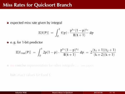
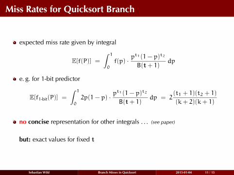
expected miss rate given by integral
E[f(P)] =
ˆ 10
f(p) · pt1(1− p)t2
B(t+ 1)dp
e. g. for 1-bit predictor
E[f1-bit(P)] =
ˆ 10
2p(1− p) · pt1(1− p)t2
B(t+ 1)dp = 2
(t1 + 1)(t2 + 1)
(k+ 2)(k+ 1)
no concise representation for other integrals . . . (see paper)
but: exact values for fixed t
Sebastian Wild Branch Misses in Quicksort 2015-01-04 11 / 15
Miss Rates for Quicksort Branch
expected miss rate given by integral
E[f(P)] =
ˆ 10
f(p) · pt1(1− p)t2
B(t+ 1)dp
e. g. for 1-bit predictor
E[f1-bit(P)] =
ˆ 10
2p(1− p) · pt1(1− p)t2
B(t+ 1)dp = 2
(t1 + 1)(t2 + 1)
(k+ 2)(k+ 1)
no concise representation for other integrals . . . (see paper)
but: exact values for fixed t
Sebastian Wild Branch Misses in Quicksort 2015-01-04 11 / 15
Miss Rate and Branch Misses
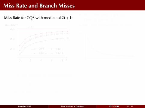
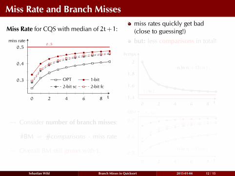
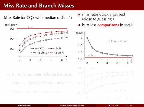
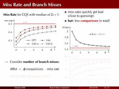
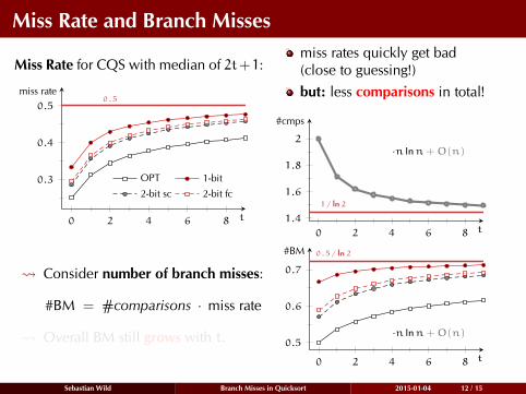
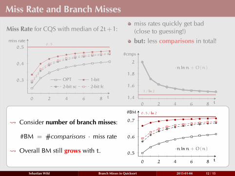
Miss Rate for CQS with median of 2t+1:
0 2 4 6 8
0.3
0.4
0.50.5
t
miss rate
OPT 1-bit
2-bit sc 2-bit fc
miss rates quickly get bad(close to guessing!)but: less comparisons in total!
0 2 4 6 8
1.4
1.6
1.8
2
1/ ln2
·n lnn+O(n)
t
#cmps
Consider number of branch misses:
#BM = #comparisons · miss rate
Overall BM still grows with t.
0 2 4 6 8
0.5
0.6
0.7
0.5/ ln2
·n lnn+O(n)
t
#BM
Sebastian Wild Branch Misses in Quicksort 2015-01-04 12 / 15
Miss Rate and Branch Misses
Miss Rate for CQS with median of 2t+1:
0 2 4 6 8
0.3
0.4
0.50.5
t
miss rate
OPT 1-bit
2-bit sc 2-bit fc
miss rates quickly get bad(close to guessing!)but: less comparisons in total!
0 2 4 6 8
1.4
1.6
1.8
2
1/ ln2
·n lnn+O(n)
t
#cmps
Consider number of branch misses:
#BM = #comparisons · miss rate
Overall BM still grows with t.
0 2 4 6 8
0.5
0.6
0.7
0.5/ ln2
·n lnn+O(n)
t
#BM
Sebastian Wild Branch Misses in Quicksort 2015-01-04 12 / 15
Branch Misses in YQS
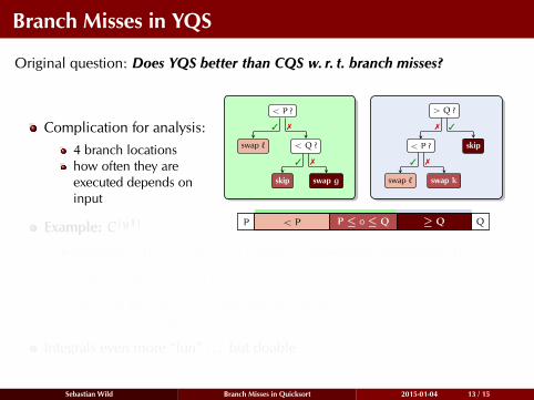
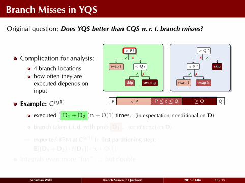
Original question: Does YQS better than CQS w. r. t. branch misses?
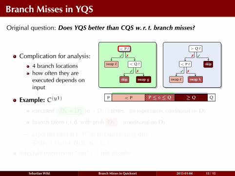
Complication for analysis:4 branch locationshow often they areexecuted depends oninput
< P ?
swap ` < Q ?
skip swap g
3 7
3 7
>Q ?
< P ? skip
swap ` swap k
37
3 7
< P P ≤ ◦ ≤ Q ≥ QP QExample: C(y1)
executed ( D1 +D2 )n+O(1) times. (in expectation, conditional on D)
branch taken i. i. d. with prob D1 . (conditional on D)
expected #BM at C(y1) in first partitioning step:E[(D1 +D2) · f(D1)] · n+O(1)
Integrals even more “fun” . . . but doable
Sebastian Wild Branch Misses in Quicksort 2015-01-04 13 / 15
Branch Misses in YQS
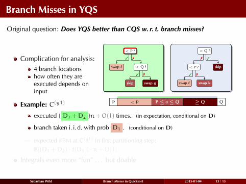
Original question: Does YQS better than CQS w. r. t. branch misses?
Complication for analysis:4 branch locationshow often they areexecuted depends oninput
< P ?
swap ` < Q ?
skip swap g
3 7
3 7
>Q ?
< P ? skip
swap ` swap k
37
3 7
< P P ≤ ◦ ≤ Q ≥ QP QExample: C(y1)
executed ( D1 +D2 )n+O(1) times. (in expectation, conditional on D)
branch taken i. i. d. with prob D1 . (conditional on D)
expected #BM at C(y1) in first partitioning step:E[(D1 +D2) · f(D1)] · n+O(1)
Integrals even more “fun” . . . but doable
Sebastian Wild Branch Misses in Quicksort 2015-01-04 13 / 15
Branch Misses in YQS
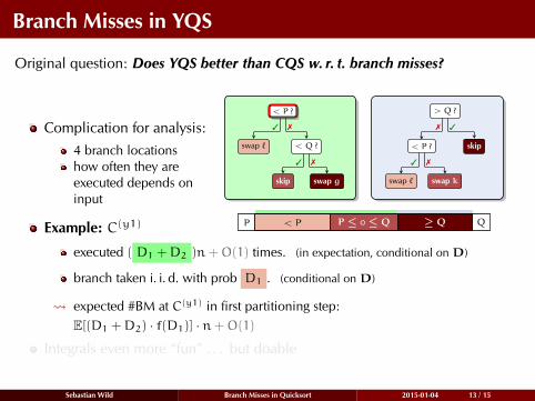
Original question: Does YQS better than CQS w. r. t. branch misses?
Complication for analysis:4 branch locationshow often they areexecuted depends oninput
< P ?
swap ` < Q ?
skip swap g
3 7
3 7
>Q ?
< P ? skip
swap ` swap k
37
3 7
< P P ≤ ◦ ≤ Q ≥ QP QExample: C(y1)
executed ( D1 +D2 )n+O(1) times. (in expectation, conditional on D)
branch taken i. i. d. with prob D1 . (conditional on D)
expected #BM at C(y1) in first partitioning step:E[(D1 +D2) · f(D1)] · n+O(1)
Integrals even more “fun” . . . but doable
Sebastian Wild Branch Misses in Quicksort 2015-01-04 13 / 15
Branch Misses in YQS
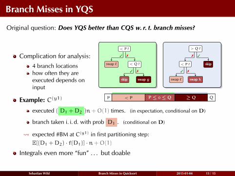
Original question: Does YQS better than CQS w. r. t. branch misses?
Complication for analysis:4 branch locationshow often they areexecuted depends oninput
< P ?
swap ` < Q ?
skip swap g
3 7
3 7
>Q ?
< P ? skip
swap ` swap k
37
3 7
< P P ≤ ◦ ≤ Q ≥ QP QExample: C(y1)
executed ( D1 +D2 )n+O(1) times. (in expectation, conditional on D)
branch taken i. i. d. with prob D1 . (conditional on D)
expected #BM at C(y1) in first partitioning step:E[(D1 +D2) · f(D1)] · n+O(1)
Integrals even more “fun” . . . but doable
Sebastian Wild Branch Misses in Quicksort 2015-01-04 13 / 15
Branch Misses in YQS
Original question: Does YQS better than CQS w. r. t. branch misses?
Complication for analysis:4 branch locationshow often they areexecuted depends oninput
< P ?
swap ` < Q ?
skip swap g
3 7
3 7
>Q ?
< P ? skip
swap ` swap k
37
3 7
< P P ≤ ◦ ≤ Q ≥ QP QExample: C(y1)
executed ( D1 +D2 )n+O(1) times. (in expectation, conditional on D)
branch taken i. i. d. with prob D1 . (conditional on D)
expected #BM at C(y1) in first partitioning step:E[(D1 +D2) · f(D1)] · n+O(1)
Integrals even more “fun” . . . but doable
Sebastian Wild Branch Misses in Quicksort 2015-01-04 13 / 15

Results CQS vs. YQS
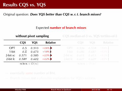
Original question: Does YQS better than CQS w. r. t. branch misses?
Expected number of branch misses
without pivot sampling
CQS YQS Relative
OPT 0.5 0.513 +2.6%
1-bit 0.6 0.673 +1.0%
2-bit sc 0.571 0.585 +2.5%
2-bit fc 0.589 0.602 +2.2%
·n lnn+O(n)
CQS median-of-3 vs. YQS tertiles-of-5
CQS YQS Relative
OPT 0.536 0.538 +0.4%
1-bit 0.686 0.687 +0.1%
2-bit sc 0.611 0.613 +0.3%
2-bit fc 0.627 0.629 +0.3%
·n lnn+O(n)
essentially same number of BM. Branch misses not a plausible explanation for YQS’s success.
Sebastian Wild Branch Misses in Quicksort 2015-01-04 14 / 15
Results CQS vs. YQS
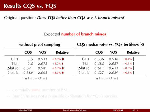
Original question: Does YQS better than CQS w. r. t. branch misses?
Expected number of branch misses
without pivot sampling
CQS YQS Relative
OPT 0.5 0.513 +2.6%
1-bit 0.6 0.673 +1.0%
2-bit sc 0.571 0.585 +2.5%
2-bit fc 0.589 0.602 +2.2%
·n lnn+O(n)
CQS median-of-3 vs. YQS tertiles-of-5
CQS YQS Relative
OPT 0.536 0.538 +0.4%
1-bit 0.686 0.687 +0.1%
2-bit sc 0.611 0.613 +0.3%
2-bit fc 0.627 0.629 +0.3%
·n lnn+O(n)
essentially same number of BM. Branch misses not a plausible explanation for YQS’s success.
Sebastian Wild Branch Misses in Quicksort 2015-01-04 14 / 15
Results CQS vs. YQS
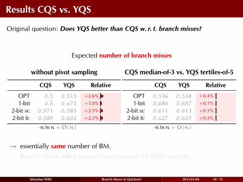
Original question: Does YQS better than CQS w. r. t. branch misses?
Expected number of branch misses
without pivot sampling
CQS YQS Relative
OPT 0.5 0.513 +2.6%
1-bit 0.6 0.673 +1.0%
2-bit sc 0.571 0.585 +2.5%
2-bit fc 0.589 0.602 +2.2%
·n lnn+O(n)
CQS median-of-3 vs. YQS tertiles-of-5
CQS YQS Relative
OPT 0.536 0.538 +0.4%
1-bit 0.686 0.687 +0.1%
2-bit sc 0.611 0.613 +0.3%
2-bit fc 0.627 0.629 +0.3%
·n lnn+O(n)
essentially same number of BM. Branch misses not a plausible explanation for YQS’s success.
Sebastian Wild Branch Misses in Quicksort 2015-01-04 14 / 15
Results CQS vs. YQS
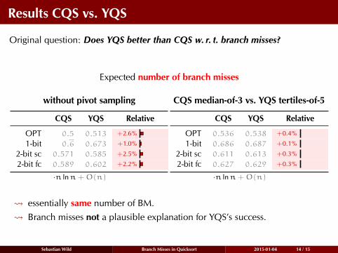
Original question: Does YQS better than CQS w. r. t. branch misses?
Expected number of branch misses
without pivot sampling
CQS YQS Relative
OPT 0.5 0.513 +2.6%
1-bit 0.6 0.673 +1.0%
2-bit sc 0.571 0.585 +2.5%
2-bit fc 0.589 0.602 +2.2%
·n lnn+O(n)
CQS median-of-3 vs. YQS tertiles-of-5
CQS YQS Relative
OPT 0.536 0.538 +0.4%
1-bit 0.686 0.687 +0.1%
2-bit sc 0.611 0.613 +0.3%
2-bit fc 0.627 0.629 +0.3%
·n lnn+O(n)
essentially same number of BM. Branch misses not a plausible explanation for YQS’s success.
Sebastian Wild Branch Misses in Quicksort 2015-01-04 14 / 15
Results CQS vs. YQS
Original question: Does YQS better than CQS w. r. t. branch misses?
Expected number of branch misses
without pivot sampling
CQS YQS Relative
OPT 0.5 0.513 +2.6%
1-bit 0.6 0.673 +1.0%
2-bit sc 0.571 0.585 +2.5%
2-bit fc 0.589 0.602 +2.2%
·n lnn+O(n)
CQS median-of-3 vs. YQS tertiles-of-5
CQS YQS Relative
OPT 0.536 0.538 +0.4%
1-bit 0.686 0.687 +0.1%
2-bit sc 0.611 0.613 +0.3%
2-bit fc 0.627 0.629 +0.3%
·n lnn+O(n)
essentially same number of BM. Branch misses not a plausible explanation for YQS’s success.
Sebastian Wild Branch Misses in Quicksort 2015-01-04 14 / 15
Conclusion
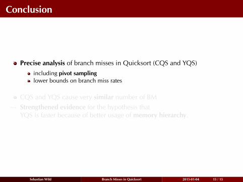
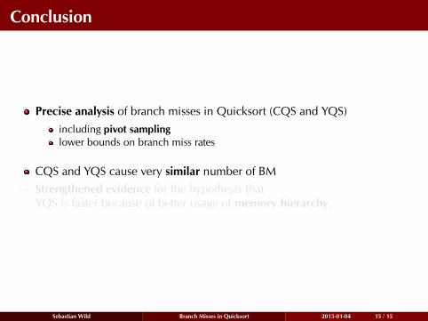
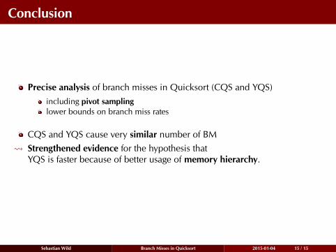
Precise analysis of branch misses in Quicksort (CQS and YQS)including pivot samplinglower bounds on branch miss rates
CQS and YQS cause very similar number of BM Strengthened evidence for the hypothesis that
YQS is faster because of better usage of memory hierarchy.
Sebastian Wild Branch Misses in Quicksort 2015-01-04 15 / 15
Conclusion
Precise analysis of branch misses in Quicksort (CQS and YQS)including pivot samplinglower bounds on branch miss rates
CQS and YQS cause very similar number of BM Strengthened evidence for the hypothesis that
YQS is faster because of better usage of memory hierarchy.
Sebastian Wild Branch Misses in Quicksort 2015-01-04 15 / 15
Miss Rate for Branches in Quicksort
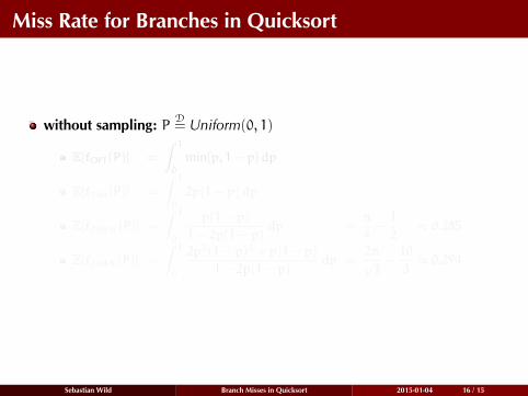
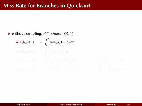
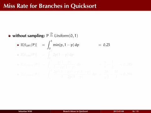
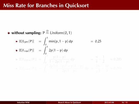
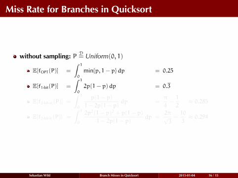
without sampling: P D= Uniform(0, 1)
E[fOPT(P)] =
ˆ 10
min{p, 1− p}dp
= 0.25
E[f1-bit(P)] =
ˆ 10
2p(1− p)dp
= 0.3
E[f2-bit-sc(P)] =
ˆ 10
p(1− p)
1− 2p(1− p)dp =
π
4−1
2≈ 0.285
E[f2-bit-fc(P)] =
ˆ 10
2p2(1− p)2 + p(1− p)
1− 2p(1− p)dp =
2π√3−10
3≈ 0.294
Sebastian Wild Branch Misses in Quicksort 2015-01-04 16 / 15
Miss Rate for Branches in Quicksort
without sampling: P D= Uniform(0, 1)
E[fOPT(P)] =
ˆ 10
min{p, 1− p}dp = 0.25
E[f1-bit(P)] =
ˆ 10
2p(1− p)dp = 0.3
E[f2-bit-sc(P)] =
ˆ 10
p(1− p)
1− 2p(1− p)dp =
π
4−1
2≈ 0.285
E[f2-bit-fc(P)] =
ˆ 10
2p2(1− p)2 + p(1− p)
1− 2p(1− p)dp =
2π√3−10
3≈ 0.294
Sebastian Wild Branch Misses in Quicksort 2015-01-04 16 / 15
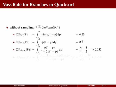
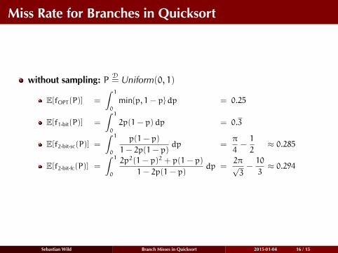