Embed Size (px)
Citation preview

A (quick) introduction to
Magnetic Resonance Imagery (MRI)
preprocessing and analysis
Stephen Larroque
Coma Science Group, GIGA research
University of Liège
24/03/2017

Outline
MRI preprocessing with SPM (long!)
VBM analysis
Functional MRI analysis with CONN
Graph Theory analysis,
by Rajanikant Panda
Diffusion MRI (DTI),
by Stephen Larroque
Parcellation and Freesurfer,
by Jitka Annen
2
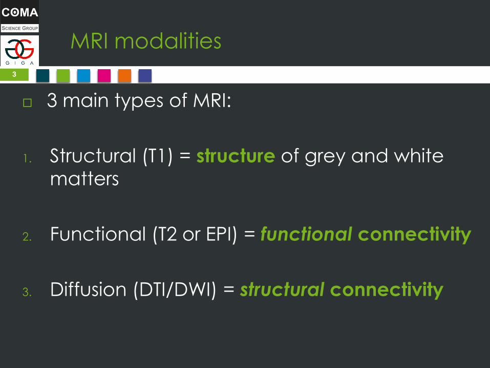
MRI modalities
3 main types of MRI:
1. Structural (T1) = structure of grey and white
matters
2. Functional (T2 or EPI) = functional connectivity
3. Diffusion (DTI/DWI) = structural connectivity
3

MRI vs fMRI
4
From Christophe Phillips course

Nomenclatura
Sequence = multiple volumes of same brain
Volume = one image of brain
Slice = one plane slice of one volume
Voxel = 3D pixel
Voxel < Slice < Volume < Sequence
5

MRI modalities
3 types of MRI:
1. Structural (T1) = 1 volume
high-resolution
2. Functional (T2 or EPI) =
sequence of volumes (low-res)
3. Diffusion (DTI/DWI) = 1 volume
but with lots of vectors (ie, as if there were cameras all around the
subject shooting all at once)
6

MRI modalities: T1 always needed
fMRI and dMRI are too low
resolution to do anything.
Solution: use T1 as a reference
= (intra-subject) coregistration
7

About SPM
SPM = Statistical Parametric Modelling
Both a software and a methodology
Freely downloadable from
www.fil.ion.ucl.ac.uk/spm/
See also documentations, articles and (video)
tutorials
We use SPM for MRI preprocessing (but can
also do analysis)
Alternatives: FSL, AFNI, BrainVoyager, Broccoli,
etc.
8

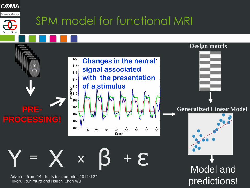
SPM model for functional MRI
Changes in the neural
signal associated
with the presentation
of a stimulus
Generalized Linear Model
Design matrix
Y = X x β + ε
Adapted from “Methods for dummies 2011-12” Hikaru Tsujimura and Hsuan-Chen Wu
Model and
predictions!
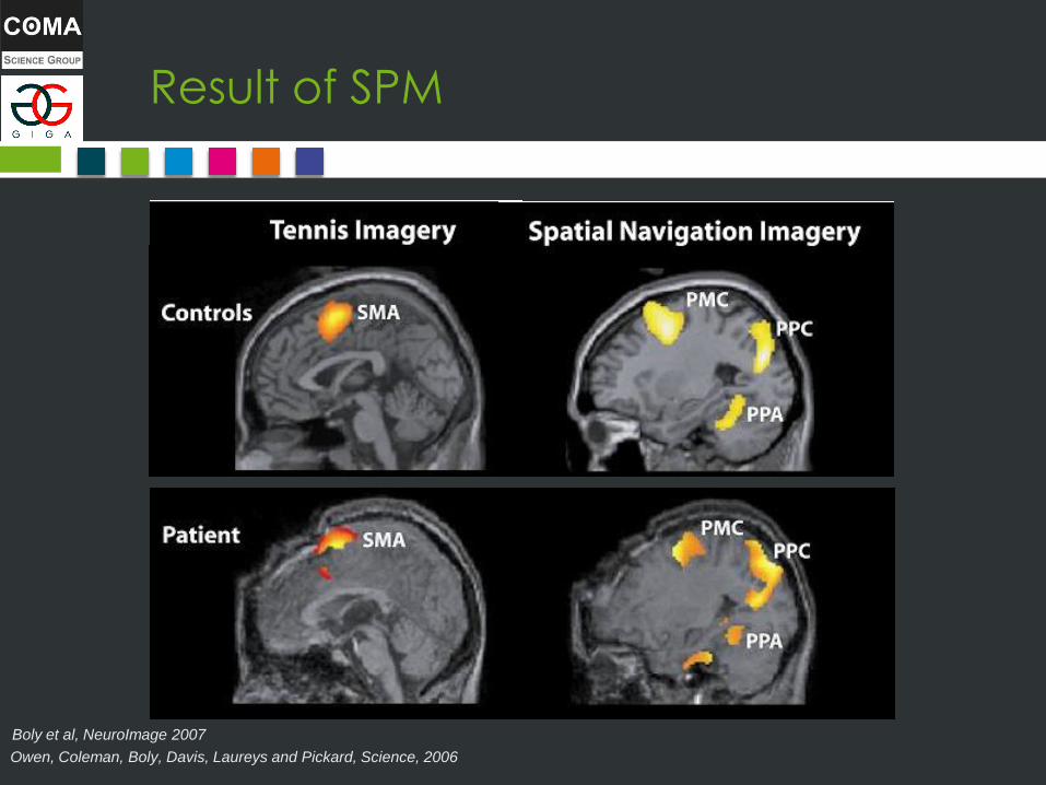
Result of SPM
• 30-seconds period of mental imagery/resting • Each imagery task was repeated 10 times.
Owen, Coleman, Boly, Davis, Laureys and Pickard, Science, 2006
Boly et al, NeuroImage 2007

SPM model for functional MRI
Changes in the neural
signal associated
with the presentation
of a stimulus
Y = X x β + ε
Adapted from “Methods for dummies 2011-12” Hikaru Tsujimura and Hsuan-Chen Wu
Generalized Linear Model
Design matrix
Model and
predictions!
SPM model for functional MRI
Changes in the neural
signal associated
with the presentation
of a stimulus
Y = X x β + ε
Adapted from “Methods for dummies 2011-12” Hikaru Tsujimura and Hsuan-Chen Wu
PRE-
PROCESSING!
Generalized Linear Model
Design matrix
Model and
predictions!
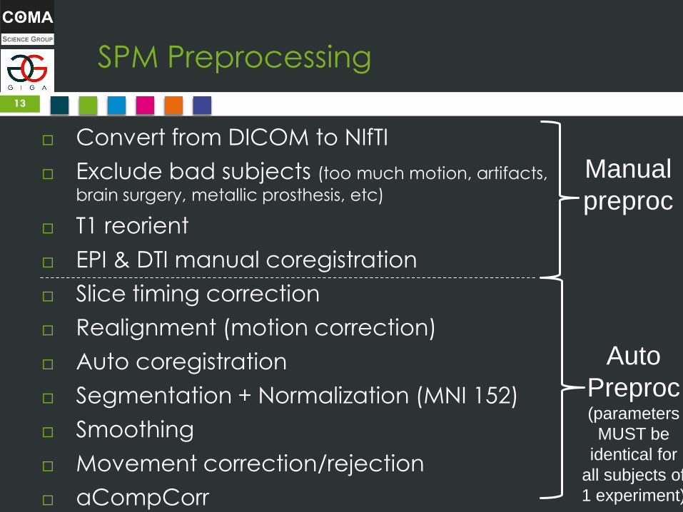
SPM Preprocessing
Convert from DICOM to NIfTI
Exclude bad subjects (too much motion, artifacts,
brain surgery, metallic prosthesis, etc)
T1 reorient
EPI & DTI manual coregistration
Slice timing correction
Realignment (motion correction)
Auto coregistration
Segmentation + Normalization (MNI 152)
Smoothing
Movement correction/rejection
aCompCorr
13
Manual
preproc
Auto
Preproc (parameters
MUST be
identical for
all subjects of
1 experiment)

Manual Preprocessing
Why? Automatic reorientation and coregistration are convex problems Multiple
local optimums
In practice: if brain is upside-down or difficult to
read, automatic algorithms will fail (but without
any error! You just get false results…)
Solution: Manually reorient and coregister, then
use automatic coregistering
Technically, this provides a better starting point
for algorithms to explore the solutions
landscape (because these algos are sensitive to initialization)
14

Manual Preprocessing - Tips
Cumbersome, but can be done as the very first
step (thus you don’t lose time waiting for
automatic steps to compute)
Keep the manually preprocessed nifti files, you
can reuse for another analysis!
15
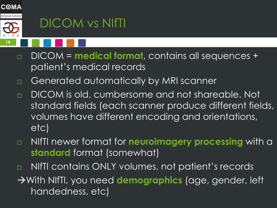
DICOM vs NIfTI
DICOM = medical format, contains all sequences +
patient’s medical records
Generated automatically by MRI scanner
DICOM is old, cumbersome and not shareable. Not
standard fields (each scanner produce different fields,
volumes have different encoding and orientations,
etc)
NIfTI newer format for neuroimagery processing with a
standard format (somewhat)
NIfTI contains ONLY volumes, not patient’s records
With NIfTI, you need demographics (age, gender, left
handedness, etc)
16

DICOM vs NIfTI - 2
Shortcomings: NIfTI strips too much info!
DICOM NIfTI always possible, but NIfTI DICOM
often impossible
An error in conversion is unrecoverable without
DICOM
See https://openfmri.org/dataset-orientation-issues/
Another example: MRIConvert will round DTI gradients
values, so bad results. Prefer mrconvert from MRTRIX3.
17

From DICOM to NIfTI
There are two NIfTI formats: 3D (1 .nii file per volume)
or 4D (1 .nii file per sequence). They are equivalent.
Use MRConvert or dcm2niix for structural and fMRI
Use MRTRIX3 mrconvert for DTI (can also be used for
structural and functional)
Or use SPM (but does not support DTI)
18

Exclude bad subjects
Rejection is CRITICAL: defines what you will get. If you
don’t reject, you will get false or no results. This cannot
be automated.
Criteria of rejection:
Demographics (underage, overage, only
representant of one gender, sedation, etc.)
Bad volumes (metal implants, acquisition artifacts due
to motion, too different brain, too much damage, …)
Bad segmentation (after preprocessing)
Too much movements (might show activity where
there’s none!) – use ART results with LRQ3000/movvis.m
19

Exclude bad subjects
Bad volumes (T1 here but check also functional and DTI)
20
Too much damages,
Will be too different from other brains
Metal implants makes MRI go crazy
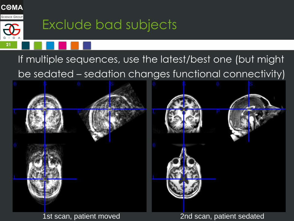
Exclude bad subjects
If multiple sequences, use the latest/best one (but might
be sedated – sedation changes functional connectivity)
21
1st scan, patient moved 2nd scan, patient sedated

Exclude bad subjects
Too much movement
22

Exclude bad subjects
Too much movement
23
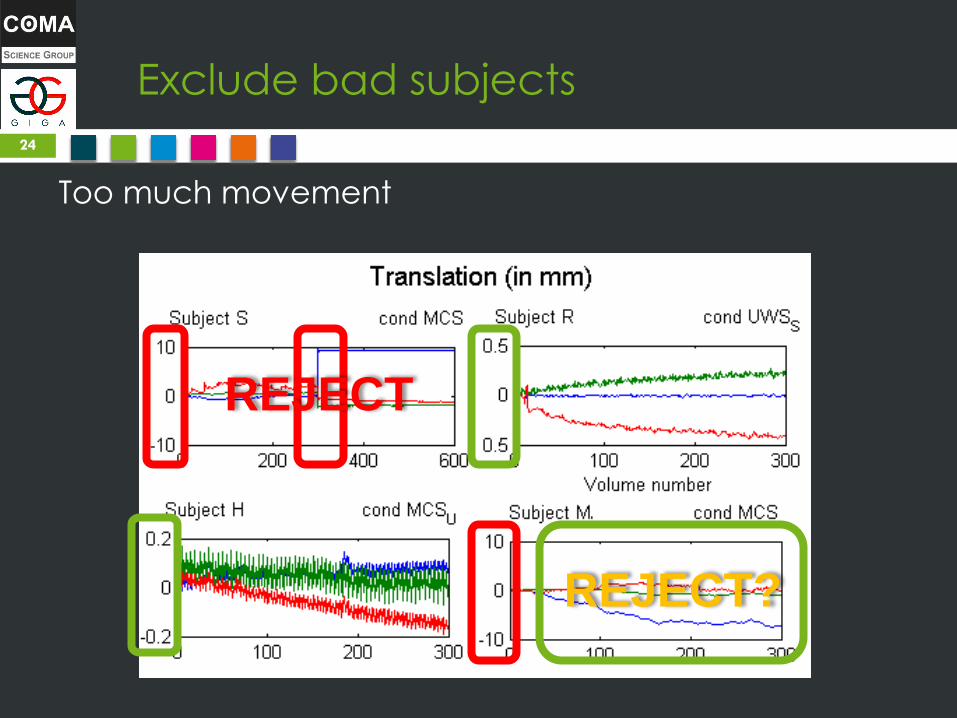
Exclude bad subjects
Too much movement
24
REJECT
REJECT?

SPM Preprocessing
Convert from DICOM to NIfTI
Exclude bad subjects (too much motion, artifacts,
brain surgery, metallic prosthesis, etc)
T1 reorient we are here
EPI & DTI manual coregistration
Slice timing correction
Realignment (motion correction)
Auto coregistration
Segmentation + Normalization (MNI 152)
Smoothing
Movement correction/rejection
aCompCorr
25
Manual
preproc
Auto
Preproc (parameters
MUST be
identical for
all subjects of
1 experiment)

SPM interface
26

SPM interface
27
• Display: T1 reorient
• Check Reg:
Manual coregistration
• Batch: all the rest
Processing progress: here
and in console
Also check console for
detailed errors!
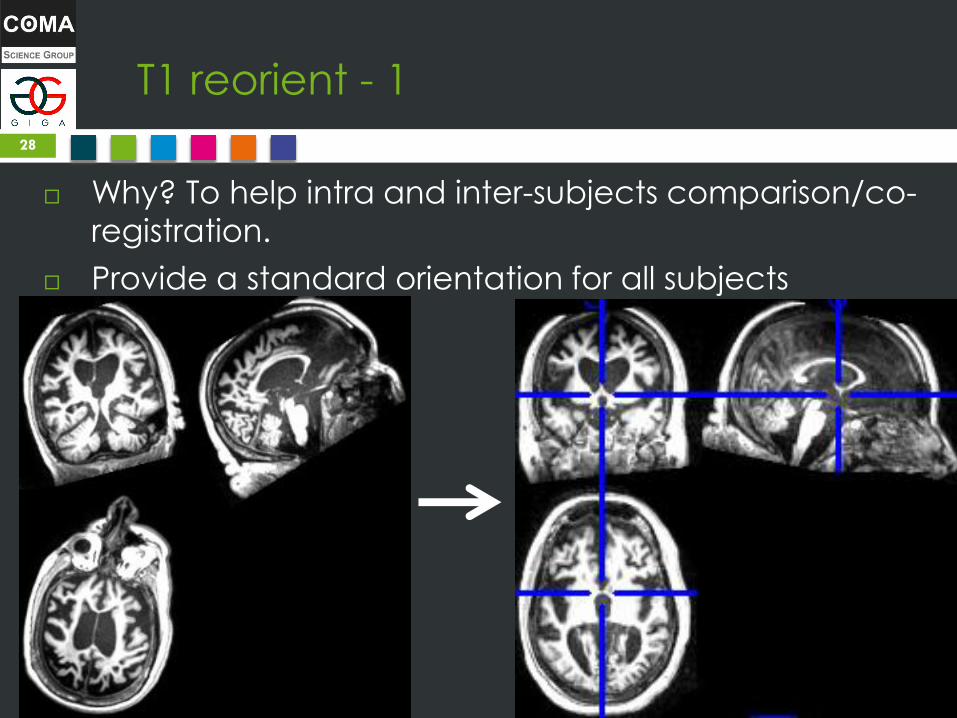
T1 reorient - 1
Why? To help intra and inter-subjects comparison/co-
registration.
Provide a standard orientation for all subjects
28

T1 reorient - 2
Our method: internal reference point AC-PC alignment
29
Estimated time:
< 3 min per subject

T1 reorient – Recipe - 1
Nomenclatura
30

T1 reorient – Recipe - 2
1. Balance eyes on view 2 & 3 for respectively yaw & roll
31
From SABRE documentation (http://sabre.brainlab.ca/docs/processing/stage3.html)

T1 reorient – Recipe - 3
2. Adjust pitch & cursor watching view 1 and 3 to get:
• A winged keyhole shape in View 3
• A extruded ball in View 1. Cursor must be on ball and top
of keyhole.
32
From SABRE documentation (http://sabre.brainlab.ca)
Bottom line
should be thin
and straight!

T1 reorient – Recipe - 4
Tip: to adjust pitch more easily, you can move cursor on
view 1 up and down, until you see the PC as a thin line.
Now, you can just adjust pitch, without moving cursor,
until the AC is in the middle of the cursor.
33
From SABRE documentation (http://sabre.brainlab.ca)

fMRI coregistration on T1
Why? To ensure good start for auto-coregistration. A
precise coregistration ensures activity is attributed to
correct region!
Estimated time: < 10 min per subject
34

fMRI coregistration on T1
35
Perfect coreg =
internal ventricules
aligned (but not
always possible,
particularly with
inhomogenous
scans)
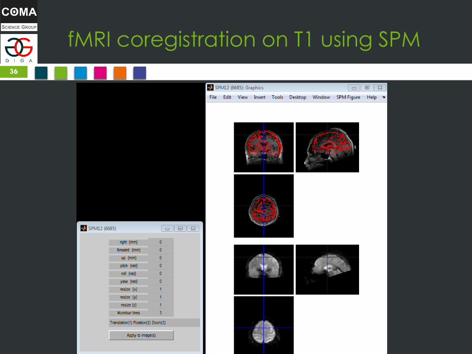
fMRI coregistration on T1 using SPM
36

fMRI coregistration on T1 - Method
Use ventricles as the guiding line to overlay T2
on T1, as ventricles are what is the closest to an
internal structure.
37
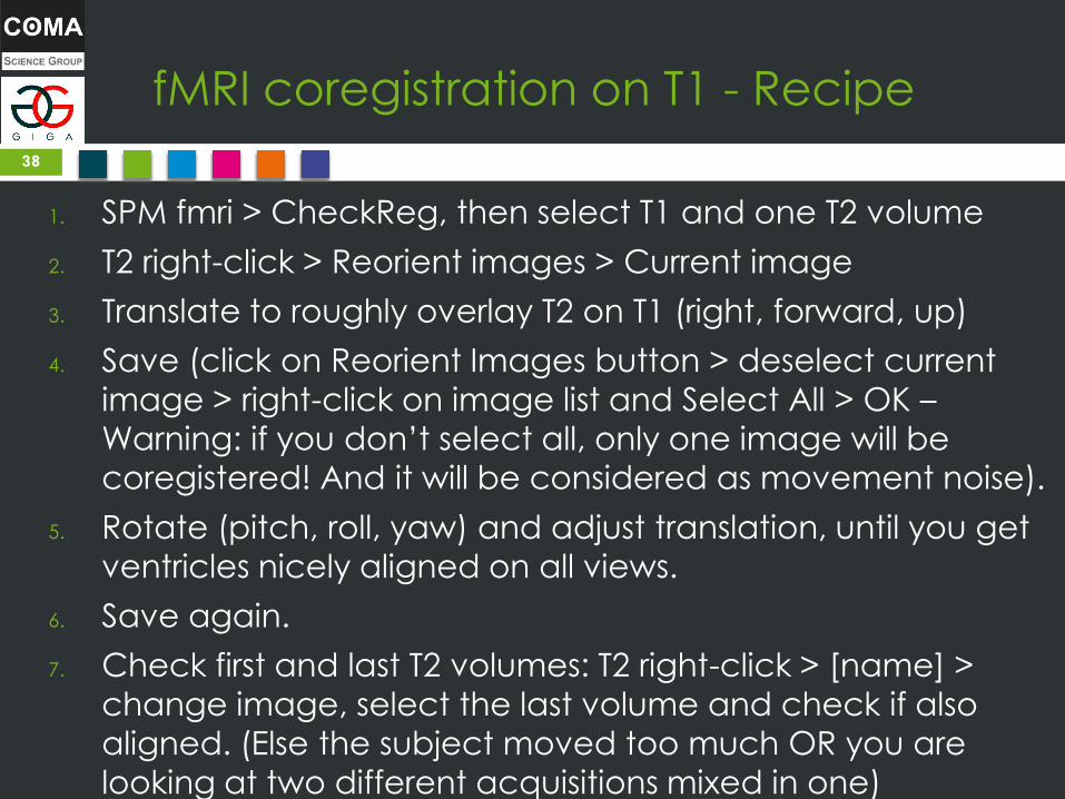
fMRI coregistration on T1 - Recipe
1. SPM fmri > CheckReg, then select T1 and one T2 volume
2. T2 right-click > Reorient images > Current image
3. Translate to roughly overlay T2 on T1 (right, forward, up)
4. Save (click on Reorient Images button > deselect current
image > right-click on image list and Select All > OK –
Warning: if you don’t select all, only one image will be
coregistered! And it will be considered as movement noise).
5. Rotate (pitch, roll, yaw) and adjust translation, until you get
ventricles nicely aligned on all views.
6. Save again.
7. Check first and last T2 volumes: T2 right-click > [name] >
change image, select the last volume and check if also
aligned. (Else the subject moved too much OR you are
looking at two different acquisitions mixed in one)
38

fMRI coregistration on T1 - Tips
Try to set #contours to 2
(instead of 3), usually ventricles
are more easy to see
If T1 intensity is too low: T1 right
click > Image > Intensity
Mapping > Local > Equalised
squared-histogram
To zoom: T2 Right-click > Zoom
> Bbox, this image nonzero OR
Bbox, this image > 100
Check ventricles alignment
not only at 1 point but over
the whole brain. Slide cursor to
animate the brain, very useful
to estimate rotation params.
39

SPM Preprocessing
Convert from DICOM to NIfTI
Exclude bad subjects (too much motion, artifacts,
brain surgery, metallic prosthesis, etc)
T1 reorient
EPI & DTI manual coregistration
Slice timing correction
Realignment (motion correction)
Auto coregistration
Segmentation + Normalization (MNI 152)
Smoothing
Movement correction/rejection
aCompCorr
40
Manual
preproc
Auto
Preproc (parameters
MUST be
identical for
all subjects of
1 experiment)
DO
NE
Automated preprocessing - 1
Slice timing correction = interpolate slices to represent
activity at identical time point. Indeed, slices are NOT
acquired at same time, so in reality a volume is composed
of several slices of slightly different time points, thus of
different activity. Slice timing correction tries to fix this.
Realignment (motion correction) = correct slight motion
artifacts between slices. Do NOT confuse with movement
correction (correct bigger motion between volumes).
Problem: doing one first will affect the other step. Thus,
neuroscientists debate (fight) about what is best.
Future solution: calculate both at the same time using a joint
optimization cost function.
Field maps = optional step just after realignment to correct
magnetic fields bias. Need to acquire a field map.
41

Precision: Slice Timing & Repetition time
Repetition time, slice scheme & order are critical infos (often not
stored in DICOMs) needed for slice timing correction. The scanning crew define them, ask them to be sure! E.g. TR=2.0s , slice scheme=72 slices singleband, slice order=ascending interleaved.
Repetition time = time between two full volumes. In other words:
this is the time it takes to acquire all slices for one volume.
Repetition time is NOT a pause, it is the cumulative sum of the
delay between each slice acquisition.
Leads to a paradox: Last slice of volume X is the closest slice (in
time and neural activity) to the first slice of next volume X+1! Hence the need for slice timing correction!
42
Automated preprocessing - 2
Automatic coregistration = like manual coreg but better at fine-tuning (but worse than human to roughly overlay).
Segmentation = separating grey matter (GM), white matter (WM) and cerebro-spinal fluid (CSF = ventricles). Tips: CSF can be used as exclusion mask, GM mask will be used by VBM and CONN. Always done on T1. NB: Skull-stripping is done here implicitly.
Normalization (to MNI) = transform brain’s shape (affine or non-linear) to overlay subjects between groups. For this, we use a template generated on lots of subjects, usually MNI (152 subjects). Always done on T1 (same transform will be applied to T2 thanks to
coregistration, with no loss of precision – if coregistration was done right ).
Segmentation and normalization are very close processes mathematically, thus there are two main approaches:
• SPM “Unified segmentation”, using Tissue Probability Maps (TPM). Most modern, using bayesian inference. But hard to adapt on brain damaged patients.
• Old segmentation using a “study-template”, generated on your own dataset (or if healthy subjects, can use SPM T1.nii template).
43

Automated preprocessing - 3
Smoothing = “blurring” final normalized T1 & T2 images to
increase SNR (signal-to-noise ratio), at the expense of specifity More significance, but less precise localization of
activity and correlations.
Usually: 8³ FWHM for healthy, 12³ for brain damage patients.
Movement correction/rejection = detect big motion
between volumes. Use NITRC ART toolbox. Use movvis.m to
visualize (all is stored in a .txt file).
44

Automated preprocessing - 4
Can also delete just the volumes where too much
movement (if still got enough volumes, above threshold for
statistical correctness: add ref, eg, for TR 2.0: 5 minutes mini).
45
Can cut here (either before or after)

Automated preprocessing - 5
aCompCor (Component Based Noise Reduction, Behzadi et
al, 2007) = alternative to signal regression, useful to get
meaningful anticorrelations (negative connectivity =
increase of anti-synchronized connectivity) in contrasts.
Indeed, anticorrelations produced after signal regression
can be due to noise (Muschelli et al, 2014).
Included in CONN “denoise” step.
46

SPM Preprocessing
Convert from DICOM to NIfTI
Exclude bad subjects (too much motion, artifacts,
brain surgery, metallic prosthesis, etc)
T1 reorient
EPI & DTI manual coregistration
Slice timing correction
Realignment (motion correction)
Auto coregistration
Segmentation + Normalization (MNI 152)
Smoothing
Movement correction/rejection
aCompCorr
47
Manual
preproc
Auto
Preproc (parameters
MUST be
identical for
all subjects of
1 experiment)
DO
NE
D
ON
E

Always CHECK
Bad T1
Movement records by ART
Segmented images (GM is correctly segmented away from
WM?)
Normalized images (not too deformed compared to original
T1?)
Etc.
48

WARNING: Last point of rejection
After automated preprocessing is the last point where you
can still reject subjects.
After this point, you begin analysis, and you can NOT reject
any subject anymore, else you are p-hacking.
You can reject one or two subjects to match gender and
age (ie, no significance in T-Test) to avoid using regressors
(to decrease degrees of flexibility and thus increase
significance), but only BEFORE analysis, NOT AFTER!
Note: you can test different pipelines and compare at this
point, but NOT after generating results, and as long as the
pipeline is applied to all subjects!
Same for smoothing: do not mix images with different
smoothing, nor with different pipelines: use the same
pipeline for all subjects
49

VBM analysis
Voxel-based morphometry (VBM) = compare
increases/decreases of brain tissue between two groups.
We compare the voxels of T1, while respecting shape of GM.
Whole-brain analysis (no seed).
Need only T1 (manual and auto preprocessing).
50
From Zurich SPM Course 2015 by Ged Ridgway (Oxford & UCL)

Functional analysis
Functional analysis = studying functional connectivity
Infer from neural signal (brain “activity”) functional connectivity by looking at correlations of activity between brain regions (ie, synchronized activity).
Capture temporality (but low-resolution).
Limitations: BOLD (Blood-Oxygen-Level Dependent) signal, not neural signal: BOLD = convol(haemodynamic response , neural signal)
SPM can model and regress haemodynamic response (up to an extent). Always think about haemodynamic response impact in your results!
Compare with:
• M/EEG: capture neural signal directly (change of potential) with high temporal resolution (but low spatial).
• PET: capture radioactive emissions of a biomarker (eg, glucose).
51

Functional analysis: paradigms &
design matrix
1st-level analysis: Look at the activity of each voxel for each
time points for one subject.
2nd-level analysis: Either:
• Inter-subjects (or between-subjects): compare between two groups (need normalization) two-tailed t-test.
• Intra-subject (or within-subject): compare across sessions for same subject (eg, before and after drug administration) paired t-test.
3rd-level: both intra and inter-subjects (multiple groups and multiple sessions
per subject). SPM does NOT support this, use CONN or manual scripts.
Task-based vs resting-state (rsfMRI) paradigms define design matrix:
• Task-based: subject is acquired in at least two sessions: one without
doing anything (resting-state) and one doing the required task. Use 2nd-
level intra-subject analysis or 3rd-level.
• Resting-state: subject is acquired 5 to 10 min doing nothing, with eyes
either closed or open (need to fix this in protocol, changes results). Use
2nd-level inter-subjects on 3rd-level.
52

Functional analysis: paradigms &
design matrix
Design matrix for n subjects doing task (two sessions):
53

Result of SPM
• 30-seconds period of mental imagery/resting • Each imagery task was repeated 10 times.
Owen, Coleman, Boly, Davis, Laureys and Pickard, Science, 2006
Boly et al, NeuroImage 2007

Model error in ResMS.nii
Residual error =
residual activity
which cannot be
explained by the
model (check the
design matrix!)
Note the max value
is very low (so we
are OK).

SPM model = learning to predict neural
stimuli
Changes in the neural
signal associated
with the presentation
of a stimulus
+
Adapted from “Methods for dummies 2011-12” Hikaru Tsujimura and Hsuan-Chen Wu
PRE-
PROCESSING!
Generalized Linear Model
Design matrix
Model and
predictions!
Y = X x β ε

SPM model = learning to predict neural
activity from stimuli
Changes in the neural
signal associated
with the presentation
of a stimulus
Y = X x β + ε
Adapted from “Methods for dummies 2011-12” Hikaru Tsujimura and Hsuan-Chen Wu
PRE-
PROCESSING!
Generalized Linear Model
Design matrix
Learn (Betas, GLM) to predict Y (neural
signal) using X (design matrix).
Map design matrix (stimuli) to neural
signal changes!
Y
X
β

SPM model = learning to predict neural
activity from stimuli
• From stimuli, can we predict a typical brain response?
That’s exactly the hypothesis of SPM.
• You (the experimenter) assume there is a link between
stimuli and brain response
• SPM will learn the model (if there is one) for you
• If no model can fit, then stimuli is not related to recorded
brain response

Linear model v. Generalized Linear Model
59
Y = x0 + x1*β1 + x2*β2 + … Y = f’(x0 + x1*β1 + x2*β2 + …) where f() is the link function
Noise ~ Normal distribution Noise ~ Link function distribution
How to know noise distribution? Visualize data and use descriptive stats!

SPM model: Why?
Neural brain activity = high dimensional data (1 voxel
= 1 feature, eg if 1 volume you have 30x30x30 = 27K! And
that’s just for 1 volume, count for a whole sequence!)
Classical statistics (hypothesis testing, contrasts, etc)
can only work when n > p (~5p <= n, where p is
number of features and n number of samples, so you
need at least 5 samples per dimension).
Machine learning statistics is better fit to high
dimension data (sparsity with L1, etc.)
SPM uses ML (regression) to reduce dimensionality
Then can use classical statistics
Contrasts are comparing models parameters (Betas),
NOT brain activity
60

SPM model: Going further
SPM uses Generalized Linear Model to reduce
dimensionality, but you can use other machine
learning models (see ICA, SearchLight, nilearn, scikit-
learn, etc.).
We use CONN (GabLab’s Connectivity Toolbox) for
functional analysis, as it streamlines SPM analysis and
can go further (voxel-to-voxel, dynamic functional
connectivity, graph theory, etc.) with more ergonomic
interface.
61

CONN toolbox
62

Functional connectivity analyses
ROI = Region of Interest = a defined group of voxels
that you consider to be stable across all subjects.
From intensity to connectivity: Pearson correlation is
done on voxels activity across time to find regions
activating together (and thus are parts of a network).
3 main types of analysis:
Seed-to-Seed (ROI-to-ROI) = analysis of connectivity
between two ROIs across time.
Seed-to-Voxel = connectivity between one ROI and
all voxels
Voxel-to-Voxel = connectivity between each voxel
and every other voxels of the brain.
63

Functional connectivity analyses - 2
1st and 2nd (& 3rd) level analyses are both possible with functional connectivity
1st level = correlation of brain regions activity across time
2nd level = difference of 1st level between conditions (groups/sessions) = difference in the correlations of brain regions activity
Correlation = positive/synchronous/within-network connectivity
Anticorrelation = negative/alternately sync/between-network connectivity. Anticorrelation is still a correlation! Just that when one network turns on, the other one turns off, and inversely. This is not necessarily inhibition, it’s just indirect communication! Warning: need to use aCompCor (CONN denoise) to ensure anticorrelations are not due to noise!
64

Correlations/anticorrelations
Correlation = positive/synchronous/within-network
connectivity
Anticorrelation = negative/alternatively
synchronized/between-network connectivity. NB:
Anticorrelation is still a correlation! Just that when one
network turns on, the other one turns off, and
inversely. This is not necessarily inhibition, it’s just
indirect communication!
65

WARNING: Good practices
Reminder: no p-hacking, no rejection after analysis!
Multiple comparison problem: use voxel-wise FDR or FWE or cluster-wise FWE (not C-FDR) or permutation test, but nothing below! Indeed, without multiple comparison correction (p-uncorrected), you will ALWAYS find something!
Multiple comparison problem (again): FDR/FEW correction does NOT PROTECT against multiple comparison! If you test lots/all seeds, you also do multiple comparison! Define beforehand max 4/5 seeds to explore, and STICK TO IT! Or apply multiple comparison at seed level: FWE = simply dividing p-values by number of seeds explored.
66

WARNING: Good practices - 2
Exploring multiple seeds being bad practice might
seem counter-intuitive
Why clicking to explore results that have already been
computed would skew the validity?
Because clicking generates new results: clicking is like
launching a coin:
67
I win if with 1 launch, I get tails:
50% chances vs
I win if, with as many launches I want,
I get tails:
• 1st launch: 50% chances
• 2nd launch: 50+25=75% chances
• 3rd launch: 87.5% chances
• 5th launch: 96% chances
• 7th launch: 99% chances of winning
Exploring multiple seeds increases chances of getting results just by chance!

WARNING: Good practices - 3
Statistical validity might seem a daunting task
In case of doubt, ask a statistician…
… and look for seminars to learn statistical literacy
Statistical literacy is the ability to understand statistics (ie, when one tool should be used, what are the limitations, etc.) in other words, to develop intuition
Noone would write in a language without understanding its words, but no need to be an expert writer
Statistics are the same: it is possible to understand and get intuition without mastering statistics: the goal is not to be able to derive calculations manually nor to prevent any issue (honest mistakes happen), but just the most common ones
68

At the end of analysis
Check ResMS.nii max value: your model is as good as low
your error is. If error is high, your model can be meaningless!
Check standard functional connectivity results: check that
controls show DMN, or other network of interest. Compare to
literature. If not, either your preprocessing/analysis is buggy,
or your MRI scanner has vibrational artifacts or worse (then
call MRI IT guys to fix that).
Ensure reproducibility: Archive (zip) your progress at at least
3 points:
• Original DICOM files (non anonymized if possible – anonymization might lose critical info).
• After manual preprocessing and before auto preprocessing.
• After whole analysis: zip both auto preprocessed files + SPM/CONN
projects + scripts/jobs used (with all the parameters you used!).
69

Thank you for your
attention Resources:
•Andy’s brain blog & youtube channel
•SPM advanced video tutorials (2011): http://www.fil.ion.ucl.ac.uk/spm/course/video/
•SPM annotated bibliography
•CONN manual (explains very well seed-to-voxel and voxel-to-voxel approaches and
measures •Consult community forums/mailing-list (mrtrix, spm, conn) and ask if necessary!
Courses at Ulg (try to find similar ones close to your university): •SPM course by Christophe Phillips
•Multivariate statistics by Gentiane Haesbroeck
•Learning the CONN toolbox by GabLab
•Neuroimagery course (about MRI technical inner workings etc)
70

BONUS SLIDES

Field maps resources
Field maps tutorials:
• https://en.wikibooks.org/wiki/Neuroimaging_Data_Processing/Field_m
ap_correction#SPM
• http://www.fil.ion.ucl.ac.uk/spm/data/fieldmap/
• Essentially: after realignment, use field map toolbox to generate a vdm
file, and use “Apply VDM” to apply it on functional volumes.
Alternative way is, instead of using “Apply VDM”, to supply the vdm file
in realignment so you can do it at the same time, but this does not
support dynamic correction (more complex acquisition schemes) like RL, high field fMRI (ie, above 3.5T), etc.
72

Neuroimagery analyses outline
73