Embed Size (px)
Citation preview

Methods to enhance the validity of precision guidelines emerging from big data
Chirag J PatelLorenzini Foundation; Venice, Italy
06/16/16
[email protected]@chiragjp
www.chiragjpgroup.org

Data streams in public health are getting large!
Capacity to measure and compute becoming high-throughput and cheaper.

Data streams in public health are getting large!
Capacity to measure and compute becoming high-throughput and cheaper.
N=500,000 1M genetic variants
1000s of phenotypes

Data streams in public health are getting large!
…and alternative data sets (e.g., EMR) are omnipresent!
image: Stan Shaw (MGH)

And new concepts for discovery:The exposome, an analog of the genome!
what to measure? how to measure?
www.sciencemag.org SCIENCE VOL 330 22 OCTOBER 2010 461
PERSPECTIVES
Xenobiotics
Inflammation
Preexisting disease
Lipid peroxidation
Oxidative stress
Gut flora
Internal
chemical
environment
External environm
ent
ExposomeRADIATION
DIET
POLLUTION
INFECTIONS
DRUGS
LIFE-STYLE
STRESS
Reactive electrophiles
Metals
Endocrine disrupters
Immune modulators
Receptor-binding proteins
critical entity for disease eti-ology ( 7). Recent discussion has focused on whether and how to implement this vision ( 8). Although fully charac-terizing human exposomes is daunting, strategies can be developed for getting “snap-shots” of critical portions of a person’s exposome during different stages of life. At one extreme is a “bottom-up” strategy in which all chemi-cals in each external source of a subject’s exposome are measured at each time point. Although this approach would have the advantage of relat-ing important exposures to the air, water, or diet, it would require enormous effort and would miss essential compo-nents of the internal chemi-cal environment due to such factors as gender, obesity, infl ammation, and stress. By contrast, a “top-down” strat-egy would measure all chem-icals (or products of their downstream processing or effects, so-called read-outs or signatures) in a subject’s blood. This would require only a single blood specimen at each time point and would relate directly to the person’s internal chemical environ-ment. Once important exposures have been identifi ed in blood samples, additional test-ing could determine their sources and meth-ods to reduce them.
To make the top-down approach feasible, the exposome would comprise a profi le of the most prominent classes of toxicants that are known to cause disease, namely, reactive elec-trophiles, endocrine (hormone) disruptors, modulators of immune responses, agents that bind to cellular receptors, and metals. Expo-sures to these agents can be monitored in the blood either by direct measurement or by looking for their effects on physiological pro-cesses (such as metabolism). These processes generate products that serve as signatures and biomarkers in the blood. For example, reac-tive electrophiles, which constitute the largest class of toxic chemicals ( 6), cannot generally be measured in the blood. However, metabo-lites of electrophiles are detectable in serum ( 9), and products of their reactions with blood nucleophiles, like serum albumin, offer possi-ble signatures ( 10). Estrogenic activity could be used to monitor the effect of endocrine dis-
ruptors and can be measured through serum biomarkers. Immune modulators trigger the production of cytokines and chemokines that also can be measured in serum. Chemicals that bind to cellular receptors stimulate the production of serum biomarkers that can be detected with high-throughput screens ( 11). Metals are readily measured in blood ( 12), as are hormones, antibodies to pathogens, and proteins released by cells in response to stress. The accumulation of biologically important exposures may also be detected as changes to lymphocyte gene expression or in chemical modifi cations of DNA (such as methylation) ( 13).
The environmental equivalent of a GWAS is possible when signatures and biomarkers of the exposome are characterized in humans with known health outcomes. Indeed, a rel-evant prototype for such a study examined associations between type 2 diabetes and 266 candidate chemicals measured in blood or urine ( 14). It determined that exposure to cer-tain chemicals produced strong associations with the risk of type 2 diabetes, with effect sizes comparable to the strongest genetic loci reported in GWAS. In another study, chromo-
some (telomere) length in peripheral blood mono-nuclear cells responded to chronic psychological stress, possibly mediated by the production of reac-tive oxygen species ( 15).
Characterizing the exposome represents a tech-
nological challenge like that of the human genome project, which began when DNA sequencing was in its infancy ( 16). Analyti-cal systems are needed to pro-cess small amounts of blood from thousands of subjects. Assays should be multiplexed for mea-suring many chemicals in each class of interest. Tandem mass spectrometry, gene and protein chips, and microfl uidic systems offer the means to do this. Plat-forms for high-throughput assays should lead to economies of scale, again like those experienced by the human genome project. And because exposome technologies would provide feedback for thera-peutic interventions and personal-ized medicine, they should moti-vate the development of commer-cial devices for screening impor-tant environmental exposures in blood samples.
With successful characterization of both exposomes and genomes, environmental and genetic determinants of chronic diseases can be united in high-resolution studies that examine gene-environment interactions. Such a union might even push the nature-ver-sus-nurture debate toward resolution.
References and Notes
1. P. Lichtenstein et al., N. Engl. J. Med. 343, 78 (2000). 2. L. A. Hindorff et al., Proc. Natl. Acad. Sci. U.S.A. 106,
9362 (2009). 3. W. C. Willett, Science 296, 695 (2002). 4. P. Vineis, Int. J. Epidemiol. 33, 945 (2004). 5. I. Dalle-Donne et al., Clin. Chem. 52, 601 (2006). 6. D. C. Liebler, Chem. Res. Toxicol. 21, 117 (2008). 7. C. P. Wild, Cancer Epidemiol. Biomarkers Prev. 14, 1847
(2005). 8. http://dels.nas.edu/envirohealth/exposome.shtml 9. W. B. Dunn et al., Int. J. Epidemiol. 37 (suppl. 1), i23
(2008). 10. F. M. Rubino et al., Mass Spectrom Rev. 28, 725 (2009). 11. T. I. Halldorsson et al., Environ. Res. 109, 22 (2009). 12. S. Mounicou et al., Chem. Soc. Rev. 38, 1119 (2009). 13. C. M. McHale et al., Mutat. Res. 10.1016/j.mrrev.
2010.04.001 (2010). 14. C. J. Patel et al., PLoS ONE 5, e10746 (2010). 15. E. S. Epel et al., Proc. Natl. Acad. Sci. U.S.A. 101, 17312
(2004). 16. F. S. Collins et al., Science 300, 286 (2003). 17. Supported by NIEHS through grants U54ES016115 and
P42ES04705.
Characterizing the exposome. The exposome represents the combined exposures from all sources that reach the internal chemical environment. Toxicologically important classes of exposome chemicals are shown. Signatures and biomarkers can detect these agents in blood or serum.
CR
ED
IT: N
. K
EV
ITIY
AG
ALA
/SC
IEN
CE
; (P
HO
TO
CR
ED
ITS
) (L
EF
T, T
OP
FIV
E IM
AG
ES
) T
HIN
KS
TO
CK
.CO
M; (L
EF
T, T
WO
IM
AG
ES
FR
OM
BO
TT
OM
) IS
TO
CK
PH
OT
O.C
OM
; (R
IGH
T) T
HIN
KS
TO
CK
PH
OT
OS
.CO
M
10.1126/science.1192603
Published by AAAS
on
Oct
ober
21,
201
0 ww
w.sc
ienc
emag
.org
Down
load
ed fr
om
how to analyze in health?
Wild, 2005Rappaport and Smith, 2010
Buck-Louis and Sundaram 2012Miller and Jones, 2014
Patel CJ and Ioannidis JPAI, 2014

Can we use these big data sources for discovery? Or, for building guidelines?

Many challenges exist in the use of big data for discovery, guideline development, and causal
researchINSIGHTS
1054 28 NOVEMBER 2014 • VOL 346 ISSUE 6213 sciencemag.org SCIENCE
In 1854, as cholera swept through Lon-
don, John Snow, the father of modern ep-
idemiology, painstakingly recorded the
locations of affected homes. After long,
laborious work, he implicated the Broad
Street water pump as the source of the
outbreak, even without knowing that a Vib-
rio organism caused cholera. “Today, Snow
might have crunched Global Positioning
System information and disease prevalence
data, solving the problem within hours” ( 1).
That is the potential impact of “Big Data” on
the public’s health. But the promise of Big
Data is also accompanied by claims that “the
scientific method itself is becoming obso-
lete” ( 2), as next-generation computers, such
as IBM’s Watson ( 3), sift through the digital
world to provide predictive models based
on massive information. Separating the true
signal from the gigantic amount of noise is
neither easy nor straightforward, but it is a
challenge that must be tackled if informa-
tion is ever to be translated into societal
well-being.
The term “Big Data” refers to volumes of
large, complex, linkable information ( 4). Be-
yond genomics and other “omic” fields, Big
Data includes medical, environmental, fi-
nancial, geographic, and social media infor-
mation. Most of this digital information was
unavailable a decade ago. This swell of data
will continue to grow, stoked by sources that
are currently unimaginable. Big Data stands
to improve health by providing insights into
the causes and outcomes of disease, better
drug targets for precision medicine, and en-
hanced disease prediction and prevention.
Moreover, citizen-scientists will increasingly
use this information to promote their own
health and wellness. Big Data can improve
our understanding of health behaviors
(smoking, drinking, etc.) and accelerate the
knowledge-to-diffusion cycle ( 5).
But “Big Error” can plague Big Data. In
2013, when influenza hit the United States
hard and early, analysis of flu-related Inter-
net searches drastically overestimated peak
flu levels ( 6) relative to those determined
by traditional public health surveillance.
Even more problematic is the potential for
many false alarms triggered by large-scale
examination of putative associations with
disease outcomes. Paradoxically, the pro-
portion of false alarms among all proposed
“findings” may increase when one can mea-
sure more things ( 7). Spurious correlations
and ecological fallacies may multiply. There
are numerous such examples ( 8), such as
“honey-producing bee colonies inversely cor-
relate with juvenile arrests for marijuana.”
The field of genomics has addressed this
problem of signal and noise by requiring
replication of study findings and by asking
for much stronger signals in terms of statisti-
cal significance. This requires the use of col-
laborative large-scale epidemiologic studies.
For nongenomic associations, false alarms
due to confounding variables or other biases
are possible even with very large-scale stud-
ies, extensive replication, and very strong
signals ( 9). Big Data’s strength is in finding
associations, not in showing whether these
associations have meaning. Finding a signal
is only the first step.
Even John Snow needed to start with a
plausible hypothesis to know where to look,
i.e., choose what data to examine. If all he
had was massive amounts of data, he might
well have ended up with a correlation as
spurious as the honey bee–marijuana con-
nection. Crucially, Snow “did the experi-
ment.” He removed the handle from the
water pump and dramatically reduced the
spread of cholera, thus moving from correla-
tion to causation and effective intervention.
How can we improve the potential for
Big Data to improve health and prevent
disease? One priority is that a stronger
epidemiological foundation is needed. Big
Data analysis is currently largely based on
convenient samples of people or informa-
tion available on the Internet. When as-
sociations are probed between perfectly
measured data (e.g., a genome sequence)
and poorly measured data (e.g., adminis-
trative claims health data), research ac-
curacy is dictated by the weakest link. Big
Data are observational in nature and are
fraught with many biases such as selection,
confounding variables, and lack of general-
izability. Big Data analysis may be embed-
ded in epidemiologically well-characterized
and representative populations. This epide-
miologic approach has served the genomics
community well ( 10) and can be extended
to other types of Big Data.
There also must be a means to integrate
knowledge that is based on a highly itera-
tive process of interpreting what we know
and don’t know from within and across sci-
entific disciplines. This requires knowledge
management, knowledge synthesis, and
knowledge translation ( 11). Curation can be
aided by machine learning algorithms. An
example is the ClinGen project ( 12) that will
create centralized resources of clinically an-
notated genes to improve interpretation
of genomic variation and optimize the use
of genomics in practice. And new funding,
such as the Biomedical Data to Knowledge
awards of the U.S. National Institutes of
Health, will develop new tools and training
in this arena.
From validity to utility. Big Data can improve tracking
and response to infectious disease outbreaks, discovery
of early warning signals of disease, and development of
diagnostic tests and therapeutics.
By Muin J. Khoury
1,2
and
John P. A. Ioannidis
3
MEDICINE
1O� ce of Public Health Genomics, Centers for Disease Control and Prevention, Atlanta, GA 30333, USA. 2Epidemiology and Genomics Research Program, National Cancer Institute, Bethesda, MD 20850, USA. 3Stanford Prevention Research Center and Meta-Research Innovation Center at Stanford, Stanford University, Palo Alto, CA 94305, USA. E-mail: [email protected]; [email protected] IL
LU
ST
RA
TIO
N:
V.
AL
TO
UN
IAN
/SCIENCE
Big data meets public healthHuman well-being could benefit from large-scale data if large-scale noise is minimized
Published by AAAS
on
June
20,
201
6ht
tp://
scie
nce.
scie
ncem
ag.o
rg/
Dow
nloa
ded
from
Science, 2014

Many challenges exist in the use of big data for discovery, guideline development, and causal research
Thousands of hypotheses are possible.Multiplicity of hypotheses.
Big data are observational.Multiplicity of biases:
confounding, selection; reverse causal
Millions of analytic scenarios are possible.Multiplicity of analytic methods.

Big data offers a multiplicity of possible hypotheses!A few examples from cohort studies
JECH, 2014

Big Data offers a multiplicity of possible hypotheses! Example: cohort database of E exposures and P phenotypes
Hum Genet 2012 JECH 2014
Curr Env Health Rep 2016
p-2
20
8
1
6
18
7
10
…
p-1
12
2
5
9
4
16
21
11
13
3
17
14
19
p
15
6 101 1482 7 …1311 12 e54 153 9 e-1e-2
…
…
…
…
E exposure factors
P ph
enot
ypic
fact
ors
which ones to test?all?
the ones in blue?
E times P possibilities!how to detect signal from noise?

Big Data offers a multiplicity of possible hypotheses!… that depends on the domain (type of measure)!
JECH, 2014National Health and Nutrition Examination
Survey (NHANES)
Big Data = Big Bias:Confounding, reverse causality, and what
causes what
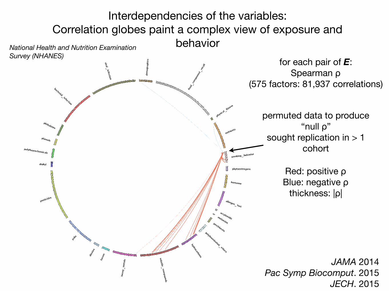
Interdependencies of the variables: Correlation globes paint a complex view of exposure and
behavior
Red: positive ρBlue: negative ρ
thickness: |ρ|
for each pair of E:Spearman ρ
(575 factors: 81,937 correlations)
permuted data to produce“null ρ”
sought replication in > 1 cohort
JAMA 2014Pac Symp Biocomput. 2015
JECH. 2015
National Health and Nutrition Examination Survey (NHANES)
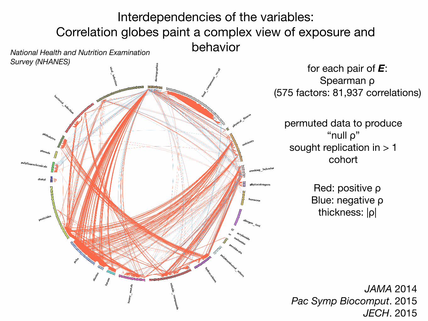
Red: positive ρBlue: negative ρ
thickness: |ρ|
for each pair of E:Spearman ρ
(575 factors: 81,937 correlations)
Interdependencies of the variables: Correlation globes paint a complex view of exposure and
behavior
permuted data to produce“null ρ”
sought replication in > 1 cohort
JAMA 2014Pac Symp Biocomput. 2015
JECH. 2015
National Health and Nutrition Examination Survey (NHANES)
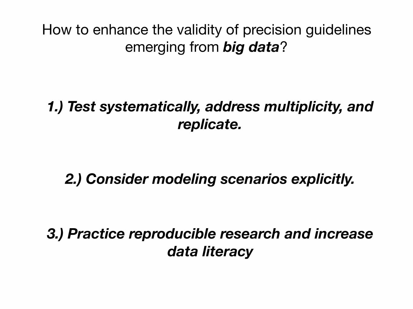
How to enhance the validity of precision guidelines emerging from big data?
1.) Test systematically, address multiplicity, and replicate.
2.) Consider modeling scenarios explicitly.
3.) Practice reproducible research and increase data literacy

Test systematically and replicate. Examples: “environment-wide” or “nutrient-wide”
association studies

A search engine for robust, reproducible genotype-phenotype associations…
580 VOLUME 42 | NUMBER 7 | JULY 2010 NATURE GENETICS
A RT I C L E S
13 autosomal loci exceeded the threshold for genome-wide significance (P ranging from 2.8 × 10⁻⁸ to 1.4 × 10⁻²²) with allele-specific odds ratios (ORs) between 1.06 and 1.14 (Table 1 and Fig. 2). All signals remained close to or beyond genome-wide significance thresholds (the least significant P value was 5.2 × 10⁻⁸) when we repeated analyses after implementing a second (post meta-analysis) round of genomic control adjustment within stage 1 data (Supplementary Note).
We extended our search for susceptibility signals to the X chromo-some, identifying one further signal in the stage 1 discovery samples meeting our criteria for follow-up (represented by rs5945326, near DUSP9, P = 2.3 × 10⁻⁶). This SNP showed strong evidence for replication in 8,535 cases and 12,326 controls (OR (allowing for X-inactivation) 1.32 (95% CI 1.16–1.49), P = 2.3 × 10⁻⁵), for a combined association P value of 3.0 × 10⁻¹⁰ (OR 1.27 (95% CI 1.18–1.37)) (Table 1 and Fig. 2).
Fourteen signals reaching genome-wide significanceTwo of the 14 signals reaching genome-wide significance on joint analysis (those near MTNR1B and IRS1) represent loci for which T2D associations have been recently reported in samples which partially overlap with those studied here10,14–16 (Table 1).
A third signal (rs231362) on 11p15 overlaps both intron 11 of KCNQ1 and the KCNQ1OT1 transcript that controls regional imprint-ing17 and influences expression of nearby genes including CDKN1C, a known regulator of beta-cell development18. This signal maps ~150 kb from T2D-associated SNPs in the 3 end of KCNQ1 first identified in East Asian GWA scans8,9. SNPs within the 3 signal were also detected in the current DIAGRAM+ meta-analysis (for example, rs163184, P = 6.8 × 10⁻⁵), but they failed to meet the threshold for initiating replication. A SNP in the 3 region (rs2237895) that was reported to reach genome-wide significance in Danish samples9 was neither typed nor imputed in the DIAGRAM+ studies. In our European-descent samples, rs231362 and SNPs in the 3 signal were not correlated
(r2 < 0.05), and conditional analyses (see below) establish these SNPs as independent (Fig. 2 and Supplementary Table 4). Further analysis in Icelandic samples has shown that both associations are restricted to the maternally transmitted allele11. Both T2D loci are independent of the common variant associations with electrocardiographic QT intervals that map at the 5 end of KCNQ1 (r2 < 0.02, D < 0.35 in HapMap European CEU data)19,20 (Supplementary Table 5).
Of the remaining loci, two (near BCL11A and HNF1A) have been highlighted in previous studies7,21–23 but are now shown to reach genome-wide significance. Rare mutations in HNF1A account for a substantial proportion of cases of maturity onset diabetes of the young, and a population-specific variant (G319S) influences T2D risk in Oji-Cree Indians24. Confirmation of a common variant association at HNF1A brings to five the number of loci known to harbor both rare mutations causal for monogenic forms of diabetes and common vari-ants predisposing to multifactorial diabetes, the others being PPARG, KCNJ11, WFS1 and HNF1B. A T2D association in the BCL11A region was suggested by the earlier DIAGRAM meta-analysis (rs10490072, P = 3 × 10⁻⁵), but replication was inconclusive7; there is only modest linkage disequilibrium (LD) between rs10490072 and the lead SNP from the present analysis (rs243021, r2 = 0.22, D = 0.73 in HapMap CEU).
The remaining nine signals map near the genes HMGA2, CENTD2, KLF14, PRC1, TP53INP1, ZBED3, ZFAND6, CHCHD9 and DUSP9 (Table 1 and Figs. 1 and 2) and represent new T2D risk loci uncovered by the DIAGRAM+ meta-analysis.
Understanding the genetic architecture of type 2 diabetesCombining newly identified and previously reported loci and assuming a multiplicative model, the sibling relative risk attributable to the 32 T2D susceptibility variants described in this paper is ~1.14. With addition of the five T2D loci recently identified by the Meta-Analysis of Glucose and Insulin-related traits Consortium (MAGIC) investigators12,13 and
50 Locus established previouslyLocus identified by current studyLocus not confirmed by current study
BCL11A
THADANOTCH2
ADAMTS9
IRS1
IGF2BP2
WFS1ZBED3
CDKAL1
HHEX/IDEKCNQ1 (2 signals*: )
TCF7L2
KCNJ11CENTD2MTNR1B
HMGA2 ZFAND6PRC1
FTOHNF1B DUSP9
Conditional analysis
Unconditional analysis
TSPAN8/LGR5HNF1A
CDC123/CAMK1DCHCHD9
CDKN2A/2BSLC30A8
TP53INP1
JAZF1KLF14
PPAR
40
30
–log
10(P
)–l
og10
(P)
20
10
10
1 2 3 4 5 6 7 8Chromosome
9 10 11 12 13 14 15 16 17 18 19 20 21 22 X0
0
Suggestive statistical association (P < 1 10–5)
Association in identified or established region (P < 1 10–4)
Figure 1 Genome-wide Manhattan plots for the DIAGRAM+ stage 1 meta-analysis. Top panel summarizes the results of the unconditional meta-analysis. Previously established loci are denoted in red and loci identified by the current study are denoted in green. The ten signals in blue are those taken forward but not confirmed in stage 2 analyses. The genes used to name signals have been chosen on the basis of proximity to the index SNP and should not be presumed to indicate causality. The lower panel summarizes the results of equivalent meta-analysis after conditioning on 30 previously established and newly identified autosomal T2D-associated SNPs (denoted by the dotted lines below these loci in the upper panel). Newly discovered conditional signals (outside established loci) are denoted with an orange dot if they show suggestive levels of significance (P < 10−5), whereas secondary signals close to already confirmed T2D loci are shown in purple (P < 10−4).
Voight et al, Nature Genetics 2012N=8K T2D, 39K Controls
GWAS in Type 2 Diabetes
A prime example of systematic associations: Genome-wide association studies (GWASs)

The same can be achieved with non-genetic factors.Example: Exposures and behaviors in mortality.

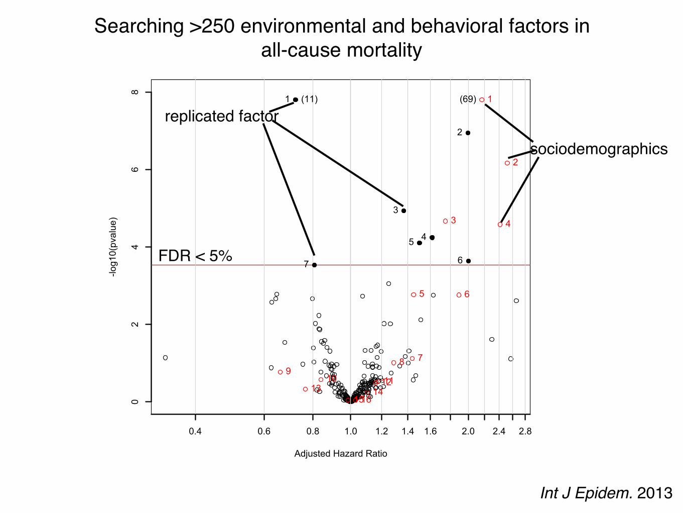
Searching for 246 exposures and behaviors associated with all-cause mortality.
NHANES: 1999-2004National Death Index linked mortality
246 behaviors and exposures (serum/urine/self-report)
NHANES: 1999-2001N=330 to 6008 (26 to 655 deaths)
~5.5 years of followup
Cox proportional hazardsbaseline exposure and time to death
False discovery rate < 5%
NHANES: 2003-2004N=177 to 3258 (20-202 deaths)
~2.8 years of followup
p < 0.05
Int J Epidem. 2013
Adjusted Hazard Ratio
-log10(pvalue)
0.4 0.6 0.8 1.0 1.2 1.4 1.6 2.0 2.4 2.8
02
46
8
1
2
3
45
67
1 Physical Activity2 Does anyone smoke in home?3 Cadmium4 Cadmium, urine5 Past smoker6 Current smoker7 trans-lycopene
(11) 1
2
3 4
5 6
789
10 111213 141516
1 age (10 year increment)2 SES_13 male4 SES_05 black6 SES_27 SES_38 education_hs9 other_eth10 mexican11 occupation_blue_semi12 education_less_hs13 occupation_never14 occupation_blue_high15 occupation_white_semi16 other_hispanic
(69)
Searching >250 environmental and behavioral factors in all-cause mortality
FDR < 5%
sociodemographics
replicated factor
Int J Epidem. 2013

Adjusted Hazard Ratio
-log10(pvalue)
0.4 0.6 0.8 1.0 1.2 1.4 1.6 2.0 2.4 2.8
02
46
8
1
2
3
45
67
1 Physical Activity2 Does anyone smoke in home?3 Cadmium4 Cadmium, urine5 Past smoker6 Current smoker7 trans-lycopene
(11) 1
2
3 4
5 6
789
10 111213 141516
1 age (10 year increment)2 SES_13 male4 SES_05 black6 SES_27 SES_38 education_hs9 other_eth10 mexican11 occupation_blue_semi12 education_less_hs13 occupation_never14 occupation_blue_high15 occupation_white_semi16 other_hispanic
(69) age (10 years)
income (quintile 2)
income (quintile 1)male
black income (quintile 3)
any one smoke in home?
serum and urine cadmium[1 SD]
past smoker?current smoker?serum lycopene
[1SD]
physical activity[low, moderate, high activity]*
*derived from METs per activity and categorized by Health.gov guidelines
R2 ~ 2%
Searching >250 environmental and behavioral factors in all-cause mortality

Searching 82 dietary factors in blood pressure:INTERMAP and NHANES
criterion. In the INTERMAP test dataset, only 3 of these 11 werenominally significant (P!0.05): alcohol, urinary calcium, andurinary sodium-to-potassium ratio (Table IV in the online-onlyData Supplement). For diastolic BP, 40 dietary or supplementvariables entered the initial model, and 10 were selected by AIC(Table IV in the online-only Data Supplement). In the INTER-MAP test dataset, only alcohol intake retained nominal signifi-cance. Thus, although we have evidence pointing to someindependent effects of nutrients for systolic BP, multivariableestimates were attenuated or lost significance compared withtheir main effects documented above (Figures 2 and 3).
The absolute effect sizes (INTERMAP testing set) rangedfrom 2.06 mm Hg lower systolic BP (phosphorus) to0.81 mm Hg lower systolic BP (non-heme iron) per 1-SDdifference in nutrient variable. The effect sizes between the
INTERMAP training set and testing set were not systematicallydifferent (5 estimates were higher and 8 were lower for systolicBP). The effect sizes between nutrients obtained from foods orfrom food and supplements combined were similar in somecases (eg, phosphorus, magnesium, fiber; Tables 1 and 2),though for some tentatively validated nutrients from foods (eg,folacin, riboflavin, and thiamin) effect sizes incorporating sup-plemental and food intake were attenuated and no longerreached the FDR 5% threshold (FDR 10%, 94%, and 97% forfolacin, riboflavin, and thiamin, respectively for systolic BP(Figures 2B and 3B).
NHANESTables 1 and 2 show the associations between the tentativelyvalidated dietary factors with systolic BP and diastolic BP across
Figure 2. Volcano plot graphic showing the nutrient-wide associations with systolic blood pressure levels in INTERMAP training set fornutrients received from foods and urine excretion markers (A) and for nutrients received from foods and supplements (B). y axis indi-cates "log10(P value) of the adjusted linear regression coefficient for each of the nutrients. Horizontal (dotted) line represents the levelof significance corresponding to FDR less than 5%, and the x axis shows the effect sizes (mm Hg) per 1 SD change in the nutrient vari-able. Filled marks represent tentatively validated nutrients in the INTERMAP testing set (P!0.05). Analyses are adjusted for age, sex,reported special diet, use of dietary supplements, moderate or heavy physical activity (hours daily), doctor diagnosed cardiovasculardisease or diabetes mellitus, family history of hypertension, height, weight, and total energy intake. INTERMAP indicates InternationalCollaborative Study on Macro-/Micronutrients and Blood Pressure. FDR indicates false discovery rate.
Tzoulaki et al A Nutrient-Wide Association Study 2459
by guest on May 21, 2016http://circ.ahajournals.org/Downloaded from
Circulation. 2012
association size
FDR < 5%
R2 ~ 7%

Testing all associations systematically:Consideration of multiplicity of hypotheses and correlational web!
Explicit in number of hypotheses tested
False discovery rate; family-wise error rate;Report database size!
Does my correlation matter? How does my new correlation
compare to the family of correlations?
0.17 (e.g., carotene and diabetes)is average ρ much less than 0.17? greater?
ρ
JAMA 2014 JECH 2015
Consideration of multitude modeling scenarios. Example: Vibration of Effects, the empirical
distribution of effect sizes due to model choice

september2011 119
Multiple modelling
This problem is akin to – but less well recognised and more poorly understood than – multiple testing. For example, consider the use of linear regression to adjust the risk levels of two treatments to the same background level of risk. There can be many covariates, and each set of covariates can be in or out of the model. With ten covariates, there are over 1000 possible models. Consider a maze as a metaphor for modelling (Figure 3). The red line traces the correct path out of the maze. The path through the maze looks simple, once it is known. Returning to a linear regression model, terms can be put into and taken out of a regression model. Once you get a p-value smaller than 0.05, the model can be frozen and the model selection justified after the fact. It is easy to justify each turn.
The combination of multiple testing and multiple modelling can lead to a very large search space, as the example of bisphenol A in Box 3 shows. Such large search spaces can give small, false positive p-values somewhere within them. Unfortunately, authors and consumers are often like a deer caught in the headlights and take a small p-value as indicating a real effect.
How can it be fixed? A new, combined strategy
It should be clear by now that more than small-scale remedies are needed. The entire system of observational studies and the claims that are made from them is no longer functional, nor is it fit for purpose. What can be done to fix this broken system? There are no principled
ways in the literature for dealing with model selection, so we propose a new, composite strategy. Following Deming, it is based not upon the workers – the researchers – but on the production system managers – the funding agencies and the editors of the journals where the claims are reported.
We propose a multi-step strategy to help bring observational studies under control (see Table 2). The main technical idea is to split the data into two data sets, a modelling data set and a holdout data set. The main operational idea is to require the journal to accept or reject the paper based on an analysis of the modelling data set without knowing the results of applying the methods used for the modelling set on the holdout set and to publish an addendum to the paper giving the results of the analysis of the holdout set. We now cover the steps, one by one.
1 The data collection and clean-up should be done by a group separate from the analysis group. There can be a tempta-tion on the part of the analyst to do some exploratory data analysis during the data clean up. Exploratory analysis could lead to model selection bias.
Box 2. Publication bias
There is general recognition that a paper has a much better chance of acceptance if something new is found. This means that, for publication, the claim in the paper has to be based on a p-value less than 0.05. From Deming’s point of view5, this is quality by inspection. The journals are placing heavy reliance on a statistical test rather than examination of the methods and steps that lead to a conclusion. As to having a p-value less than 0.05, some might be tempted to game the system10 through multiple testing, multiple modelling or unfair treatment of bias, or some combination of the three that leads to a small p-value. Researchers can be quite creative in devising a plausible story to fit the statistical finding.
2 The data cleaning team creates a modelling data set and a holdout set and gives the modelling data set, less the item to be predicted, to the analyst for examination.
P < 0.05
Figure 3. The path through a complex process can appear quite simple once the path is defined. Which terms are included in a multiple linear regression model? Each turn in a maze is analogous to including or not a specific term in the evolving linear model. By keeping an eye on the p-value on the term selected to be at issue, one can work towards a suitably small p-value. © ktsdesign – Fotolia
Table 2. Steps 0–7 can be used to help bring the observational study process into control. Currently researchers analysing observational data sets are under no effective oversight
Step Process / Action
0 Data are made publicly available
1 Data cleaning and analysis separate
2 Split sample: A, modelling; and B, holdout (testing)
3 Analysis plan is written, based on modelling data only
4 Written protocol, based on viewing predictor variables of A
5 Analysis of A only data set
6 Journal accepts paper based on A only
7 Analysis of B data set gives Addendum
A maze of associations is one way to a fragmented literature and Vibration of Effects
Young, 2011
univariate
sex
sex & age
sex & race
sex & race & age
JCE, 2015

Distribution of associations and p-values due to model choice: Estimating the Vibration of Effects (or Risk)
Variable of Intereste.g., 1 SD of log(serum Vitamin D)
Adjusting Variable Setn=13
All-subsets Cox regression213+ 1 = 8,193 models
SES [3rd tertile]education [>HS]
race [white]body mass index [normal]
total cholesterolany heart disease
family heart diseaseany hypertension
any diabetesany cancer
current/past smoker [no smoking]drink 5/day
physical activity
Data SourceNHANES 1999-2004
417 variables of interesttime to death
N≧1000 (≧100 deaths)
effect sizes p-values
Vibration of EffectsRelative Hazard Ratio (RHR)=HR99/HR1
Range of P-value (RP)=-log10(p-value1) + log10(pvalue99)
●
●
●
●
●
●
●
●
●
●
●
●
●●
0
1
2
3
4
56
78 9 10
111213
1
50
99
1 50 99
2.5
5.0
7.5
0.64 0.68 0.72 0.76Hazard Ratio
−log
10(p
valu
e)
Vitamin D (1SD(log)) RHR = 1.14
RPvalue = 4.68
A
B
C D
E
F
median p-value/HR for k
percentile indicator
JCE, 2015
●
●
●
●
●
●
●
●
●
●
●
●
●●
0
1
2
3
4
56
78 9 10
111213
1
50
99
1 50 99
2.5
5.0
7.5
0.64 0.68 0.72 0.76Hazard Ratio
−log
10(p
valu
e)
Vitamin D (1SD(log)) RHR = 1.14RP = 4.68
●
●
●
●
●
●
●
●
●
●
●
●
●
●
01
2 34
56
78
910
1112
13
1
50
99
1 50 99
1
2
3
4
0.75 0.80 0.85 0.90Hazard Ratio
−log
10(p
valu
e)
Thyroxine (1SD(log)) RHR = 1.15RP = 2.90

The Vibration of Effects: Vitamin D and Thyroxine and attenuated risk in mortality
JCE, 2015
●
●
●
●
●
●
●
●
●
●
●
●
●●
0
1
2
3
4
56
78 9 10
111213
1
50
99
1 50 99
2.5
5.0
7.5
0.64 0.68 0.72 0.76Hazard Ratio
−log
10(p
valu
e)
Vitamin D (1SD(log)) RHR = 1.14RP = 4.68
●
●
●
●
●
●
●
●
●
●
●
●
●
●
01
2 34
56
78
910
1112
13
1
50
99
1 50 99
1
2
3
4
0.75 0.80 0.85 0.90Hazard Ratio
−log
10(p
valu
e)
Thyroxine (1SD(log)) RHR = 1.15RP = 2.90

●
●
●
●
●
●
●
●
●
●
●
●●
●
01
23
45
6
78
910111213
1
50
99
1 50 99
5
10
1.3 1.4 1.5 1.6Hazard Ratio
−log
10(p
valu
e)
Cadmium (1SD(log)) adjustment=drink_five_per_day
●
●
●
●
●
●
●
●
●
●
●
●●
●
01
23
45
6
78
910111213
1
50
99
1 50 99
5
10
1.3 1.4 1.5 1.6Hazard Ratio
−log
10(p
valu
e)
Cadmium (1SD(log)) adjustment=current_past_smoking
●
●
●
●
●
●
●
●
●
●
●
●●
●
01
23
45
6
78
910111213
1
50
99
1 50 99
5
10
1.3 1.4 1.5 1.6Hazard Ratio
−log
10(p
valu
e)
Cadmium (1SD(log)) RHR = 1.29RP = 8.29
The Vibration of Effects: shifts in the effect size distribution due to select adjustments (e.g., adjusting cadmium levels with
smoking status)
JCE, 2015

●●●●●●●●●●●●●● 012345678910111213 1
5099
15099
0
1
2
3
1 2 3 4 5Hazard Ratio
−log
10(p
valu
e)
marital_status(married,widow,divorced,separated,never married,with partner,refused) never married vs. married RHR = 1.43
RP = 0.49
●●●●●●●●●●●●●●
01234
5678910111213 1
50
99
15099
0
1
2
3
1 2 3 4 5Hazard Ratio
−log
10(p
valu
e)
marital_status(married,widow,divorced,separated,never married,with partner,refused) with partner vs. married RHR = 1.69
RP = 0.75
●●●●●●●●●●●●●●
012345678910111213
1
5099
1 50 99
0
1
2
3
1 2 3 4 5Hazard Ratio
−log
10(p
valu
e)
marital_status(married,widow,divorced,separated,never married,with partner,refused) refused vs. married RHR = 3.87
RP = 0.96
●
●
●
●
●● ● ● ●
●●
●●
●
01
23
4 5 6 7 8 9 10111213
1
5099
1 50 99
0.0
0.5
1.0
0.90 0.95 1.00 1.05Hazard Ratio
−log
10(p
valu
e)
Alpha−carotene (1SD(log)) RHR = 1.15RP = 0.42
●
●
●
●
●
●●●●●●
●●●
01
23
45 678910111213
1
50
99
1 50 99
0
1
2
3
0.85 0.90 0.95Hazard Ratio
−log
10(p
valu
e)
Alcohol (1SD(log)) RHR = 1.16RP = 2.41
●
●
●
●
●
●
●
●
●●
●●
●●
0
1
2
34
56
78
9 10111213
1
50
99
1 50 99
1
2
3
4
5
0.75 0.80 0.85 0.90Hazard Ratio
−log
10(p
valu
e)
Vitamin E as alpha−tocopherol (1SD(log)) RHR = 1.15RP = 3.17
●
●
●
●
●
●
●
●
●
●
●●
●●
0
1
2
3
45
67
89
10 111213
1
50
99
1 50 99
1
2
3
0.80 0.85 0.90Hazard Ratio
−log
10(p
valu
e)
Beta−carotene (1SD(log)) RHR = 1.15RP = 2.34
●●●●●●
●●●●●● ●●
01 2345678910111213
1
50
99
1 50 99
1
2
3
0.875 0.900 0.925 0.950 0.975Hazard Ratio
−log
10(p
valu
e)
Caffeine (1SD(log)) RHR = 1.10RP = 1.99
●
●
●
●
●
●
●
●●
●●
●●●
0
1
2
3
45
67
8 910111213
1
50
99
1 50 99
0.0
0.5
1.0
1.5
0.90 0.95 1.00Hazard Ratio
−log
10(p
valu
e)
Calcium (1SD(log)) RHR = 1.13RP = 1.15
●
●
●
●
●
●
●
●
●●
●●●
●
0
1
2
3
45
67
8 9 10111213
1
50
99
1 50 99
0.5
1.0
1.5
2.0
2.5
0.84 0.88 0.92Hazard Ratio
−log
10(p
valu
e)
Carbohydrate (1SD(log)) RHR = 1.12RP = 1.57
●
●
●
●
●
●
●
●●
●●
●●●
0
1
2
3
45
67 8 9
10111213
1
50
99
1 50 99
0.5
1.0
1.5
2.0
2.5
0.80 0.84 0.88Hazard Ratio
−log
10(p
valu
e)
Carotene (1SD(log)) RHR = 1.14RP = 1.53
●●●●●●●●●●●●●●
012345678910111213
1
50
99
1 50 99
0.5
1.0
1.050 1.075 1.100 1.125Hazard Ratio
−log
10(p
valu
e)
Cholesterol (1SD(log)) RHR = 1.08RP = 0.64
●
●
●
●
●
●
●
●●
●●
●●●
0
1
2
3
45
67
8 9 10111213
1
50
99
1 50 99
1
2
3
4
0.80 0.85 0.90 0.95Hazard Ratio
−log
10(p
valu
e)
Copper (1SD(log)) RHR = 1.17RP = 2.86
●
●
●
●
●
●
●
●●
●●
●●●
0
1
2
3
45
67 8 910111213
1
50
99
1 50 99
0.0
0.5
1.0
1.5
0.85 0.90 0.95 1.00Hazard Ratio
−log
10(p
valu
e)
Beta−cryptoxanthin (1SD(log)) RHR = 1.15RP = 1.39
●
●
● ● ● ●●
●●
●●
●●
●01
2 3 4 5 6 7 8 9 101112131
50
99
1 50 99
0.0
0.5
1.0
0.96 0.99 1.02 1.05 1.08Hazard Ratio
−log
10(p
valu
e)
Folic acid (1SD(log)) RHR = 1.09RP = 0.41
●
●
●
●
●
●
●●
●●
●●●
●
0
1
2
34
56
7 8 9 10111213
1
50
99
1 50 99
1
2
3
4
0.80 0.85 0.90Hazard Ratio
−log
10(p
valu
e)
Folate, DFE (1SD(log)) RHR = 1.14RP = 2.39
●
●
●
●
●
●
●
●●
●●
●●●
0
1
2
34
56
7 8 910111213
1
50
99
1 50 99
2
4
6
8
0.76 0.80 0.84 0.88Hazard Ratio
−log
10(p
valu
e)
Food folate (1SD(log)) RHR = 1.14RP = 4.64
●
●
●
●
●
●
●
●
●●
●●
●●
0
1
23
45
67
89
10111213
1
50
99
1 50 99
1
2
3
4
0.80 0.84 0.88 0.92Hazard Ratio
−log
10(p
valu
e)
Dietary fiber (1SD(log)) RHR = 1.15RP = 2.79
●
●
●
●
●
●
●
●●
●●
●●●
0
1
2
34
56
78 9 1011 1213
1
50
99
1 50 99
1
2
3
0.80 0.84 0.88 0.92 0.96Hazard Ratio
−log
10(p
valu
e)
Total Folate (1SD(log)) RHR = 1.15RP = 2.11
●
●
●
●
●
●
●
●
●
●●
●●●
0
1
23
45
67
891011
1213
1
50
99
1 50 99
1
2
0.84 0.88 0.92Hazard Ratio
−log
10(p
valu
e)
Iron (1SD(log)) RHR = 1.12RP = 1.91
β-carotene caffeine
cholesterol
food folate

●
●
●
●
●
●
●
●●
●●
●●●
0
1
2
3
45
67 8
910111213
1
50
99
1 50 99
1
2
3
0.80 0.85 0.90Hazard Ratio
−log
10(p
valu
e)
Potassium (1SD(log)) RHR = 1.14RP = 2.28
●
●
●
●
●
●
●●
●●
●●●●
01
2
34
56
7 8 910111213
1
50
99
1 50 99
0.5
1.0
1.5
2.0
0.850 0.875 0.900 0.925 0.950Hazard Ratio
−log
10(p
valu
e)
Protein (1SD(log)) RHR = 1.11RP = 1.42
●●
● ● ●●
●●
●●
●●
●●
01
2 3 4 5 6 78 910111213
1
50
99
1 50 99
0.0
0.5
1.0
0.95 1.00 1.05 1.10Hazard Ratio
−log
10(p
valu
e)
Retinol (1SD(log)) RHR = 1.13RP = 0.67
●
●
●●
●
●
●
●
●
●
●
●
●●
01
23
45
67
89
1011
1213
1
50
99
1 50 99
0.0
0.5
1.0
1.5
1.00 1.05 1.10Hazard Ratio
−log
10(p
valu
e)
SFA 4:0 (1SD(log)) RHR = 1.11RP = 1.29
●●
●
●
●
●
●●
●
●
●●
●●
01
23
45
67
89
10111213
1
50
99
1 50 99
0.5
1.0
1.5
2.0
2.5
1.04 1.08 1.12 1.16Hazard Ratio
−log
10(p
valu
e)
SFA 6:0 (1SD(log)) RHR = 1.11RP = 1.71
●●
●
●
●
●
●
●
●
●
●
●●●
01
23
45
67
89
10111213
1
50
99
1 50 99
2
3
4
1.12 1.16 1.20Hazard Ratio
−log
10(p
valu
e)
SFA 8:0 (1SD(log)) RHR = 1.10RP = 2.55
●●
●
●
●
●
●
●
●
●
●●●●
0 1
23
45
67
89
10111213
1
50
99
1 50 99
1
2
1.04 1.08 1.12 1.16Hazard Ratio
−log
10(p
valu
e)
SFA 10:0 (1SD(log)) RHR = 1.11RP = 1.87
●●
●
●●
●●
●●
●
●●●●
01
23
45
6 78 910111213
1
50
99
1 50 99
1.0
1.5
2.0
2.5
3.0
1.075 1.100 1.125 1.150 1.175Hazard Ratio
−log
10(p
valu
e)
SFA 12:0 (1SD(log)) RHR = 1.08RP = 1.79
●●
●
●●
●●
●
●●
●●●●
01
23
45
67
8 9 10111213
1
50
99
1 50 99
0.5
1.0
1.5
2.0
1.05 1.10 1.15Hazard Ratio
−log
10(p
valu
e)
SFA 14:0 (1SD(log)) RHR = 1.11RP = 1.61
●●
●
●●
●●
●●
●●
●●●
012
34
5 6 7 8 910111213
1
50
99
1 50 99
0.0
0.5
1.0
1.00 1.05 1.10Hazard Ratio
−log
10(p
valu
e)
SFA 16:0 (1SD(log)) RHR = 1.11RP = 0.84
●●
●●
●●
●●
●●● ●
●●
012 3 4 5 67 8910111213
1
50
99
1 50 99
0.0
0.5
1.0
1.02 1.06 1.10Hazard Ratio
−log
10(p
valu
e)
SFA 18:0 (1SD(log)) RHR = 1.10RP = 0.73
●
●
●
●
●
●
●●
●●●
● ●●
01
2
34
56 7 8 910111213
1
50
99
1 50 99
0.5
1.0
1.5
2.0
0.875 0.900 0.925 0.950Hazard Ratio
−log
10(p
valu
e)
Selenium (1SD(log)) RHR = 1.09RP = 1.24
●●
●
●
●
●
●●
●●
●●●●
012
34
56 7
8910
111213
1
50
99
1 50 99
0.0
0.5
1.0
1.00 1.05 1.10 1.15Hazard Ratio
−log
10(p
valu
e)
Total saturated fatty acids (1SD(log)) RHR = 1.11RP = 0.93
● ●
●●●●●●●●●●●●
0 12 345678910111213
1
50
99
1 50 99
2
4
6
0.650 0.675 0.700 0.725 0.750Hazard Ratio
−log
10(p
valu
e)
Sodium (1SD(log)) RHR = 1.12RP = 3.74
●
●
●
●
●
●
●
●●●
●●●●
0
1
23
45
67 8910111213
1
50
99
1 50 99
1
2
3
4
0.76 0.80 0.84Hazard Ratio
−log
10(p
valu
e)
Total sugars (1SD(log)) RHR = 1.13RP = 2.51
●
●● ●
●●
●●
●●
●●●●
01 2 3 4 5 6 7 8 910111213
1
50
99
1 50 99
0.0
0.5
1.0
0.95 1.00 1.05 1.10Hazard Ratio
−log
10(p
valu
e)
Total fat (1SD(log)) RHR = 1.11RP = 0.54
●
●
●
●
●
●●
●●●
●●●●
0
1
23
45 6 78910111213
1
50
99
1 50 99
0.5
1.0
1.5
0.87 0.90 0.93 0.96Hazard Ratio
−log
10(p
valu
e)
Theobromine (1SD(log)) RHR = 1.08RP = 1.19
●
●
●
●
●
●
●
●
●●
●●
●●
0
1
2
3
45
67
8 910111213
1
50
99
1 50 99
0.4
0.8
1.2
1.6
0.80 0.84 0.88 0.92Hazard Ratio
−log
10(p
valu
e)
Vitamin A (1SD(log)) RHR = 1.13RP = 1.09
●
●
●
●
●
●
●
●
●●
●●
●●
0
1
2
34
56
78
910 111213
1
50
99
1 50 99
0.0
0.5
1.0
1.5
0.85 0.90 0.95 1.00Hazard Ratio
−log
10(p
valu
e)
Vitamin A, RAE (1SD(log)) RHR = 1.16RP = 1.31
●
●
●
●
●
●
●●
●●
● ●●●
01
2
34
56 7 8 910111213
1
50
99
1 50 99
0.5
1.0
0.86 0.90 0.94 0.98Hazard Ratio
−log
10(p
valu
e)
Retinol (1SD(log)) RHR = 1.15RP = 0.74
sodium sugars
SFA 6:0
SFA 8:0 SFA 10:0
JCE, 2015
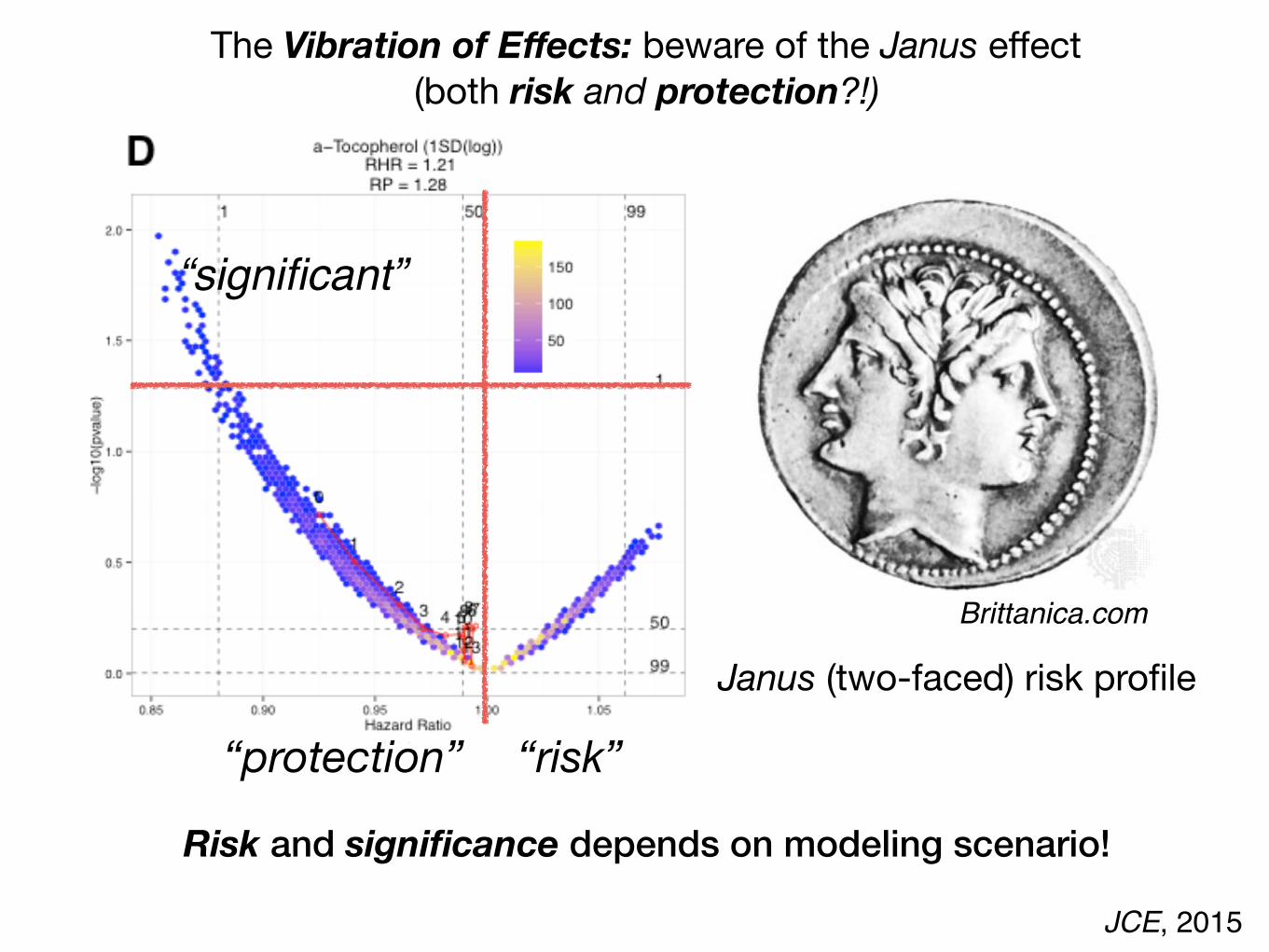
Janus (two-faced) risk profile
Risk and significance depends on modeling scenario!
The Vibration of Effects: beware of the Janus effect(both risk and protection?!)
“risk”“protection”
“significant”
Brittanica.com

Need to document analysis approach(es).
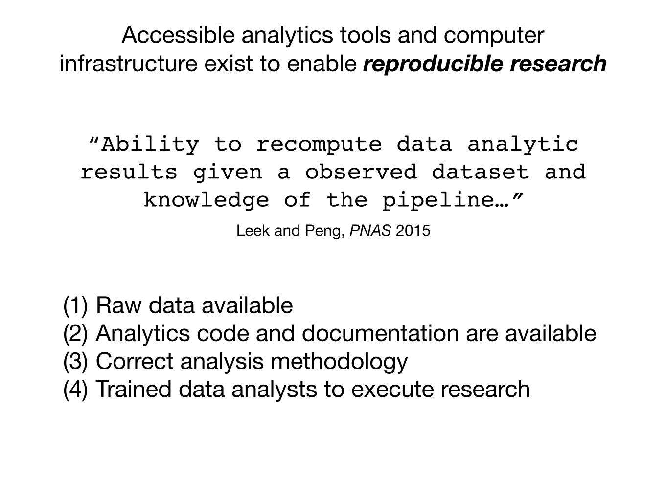
Accessible analytics tools and computer infrastructure exist to enable reproducible research
“Ability to recompute data analytic results given a observed dataset and
knowledge of the pipeline…”Leek and Peng, PNAS 2015
(1) Raw data available(2) Analytics code and documentation are available(3) Correct analysis methodology(4) Trained data analysts to execute research

http://github.comrepository to deposit and control code

“Markdown” files to document analytic process
code
output
annotation
annotation

http://chiragjpgroup.org/exposome-analytics-course

In conclusion: Big data promises multitude of ways to discover precision guidelines
Thousands of hypotheses are possible.Multiplicity of hypotheses.
Big Data are observational.Multiplicity of biases: confounding, selection; reverse causal
Millions of analytic scenarios are possible.Multiplicity of analytic methods.
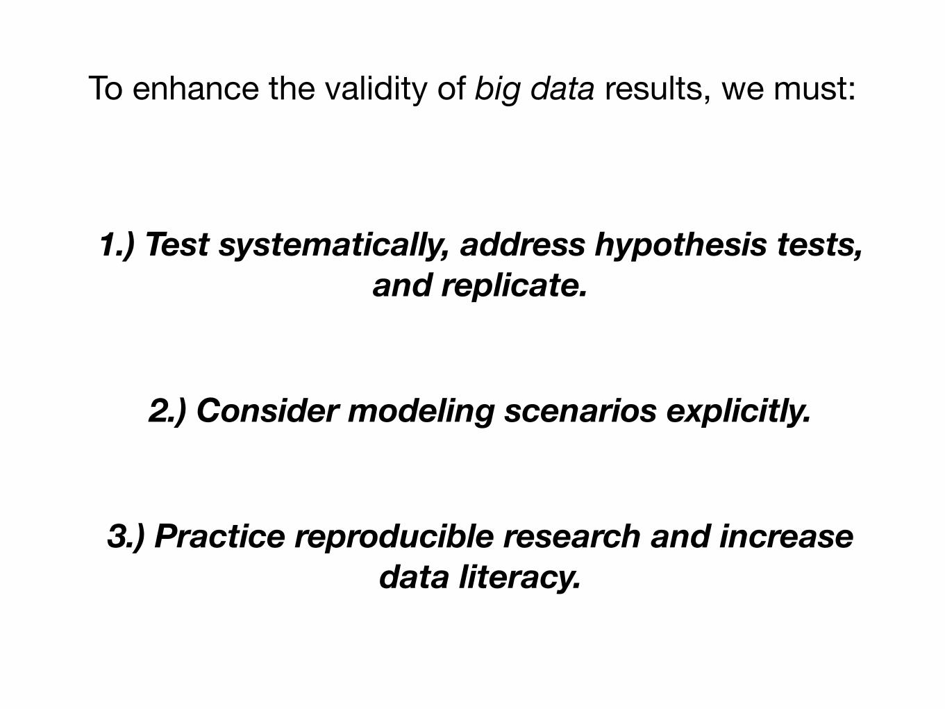
To enhance the validity of big data results, we must:
1.) Test systematically, address hypothesis tests, and replicate.
2.) Consider modeling scenarios explicitly.
3.) Practice reproducible research and increase data literacy.
Harvard DBMI Isaac KohaneSusanne ChurchillStan ShawJenn GrandfieldSunny AlvearMichal Preminger
Harvard Chan Hugues AschardFrancesca Dominici
Chirag J [email protected]
@chiragjpwww.chiragjpgroup.org
NIH Common FundBig Data to Knowledge
AcknowledgementsStanford John IoannidisAtul Butte (UCSF)
U Queensland Jian YangPeter Visscher
Cochrane Belinda Burford
RagGroup Chirag Lakhani Adam Brown Danielle RasoolyArjun ManraiErik CoronaNam Pho
Dennis Bier Emanuela Folco Elena Colombo
Lorenzini Foundation