Embed Size (px)
DESCRIPTION
Journal of applied clinical medical physics Vol 14, No 5 (2013) -- Журнал прикладной клинической медицинской физики (JACMP) публикует статьи, которые помогут клиническим медицинским физиков выполнять свои обязанности более эффективно и результативно, с большей полезностью для пациента. Журнал был основан в 2000 году, является журналом открытого доступа и публикуется дважды в месяц.
Citation preview

The future of medical physics in the US health-care systemThis issue, I would like to digress from the meaning of the JACMP and discuss with you some personal thoughts on the US health-care system and the future of medical physics under the Affordable Care Act. My credentials for discussing this topic include a newly minted PhD in Health Management from the School of Public Health at the University of Louisville. I spent many rewarding hours in classes, seminars, and lectures learning about the changes in US health care and public health over the past 11 years. This is a very difficult topic to explore in the limited space assigned to an editorial, but I would like to point out some themes that we need to bear in mind as we look forward.
1. Efficiency — It is expected that the Affordable Care Act will add approximately 30 million people to the roles of the insured. Health-care workers likely will be expected to absorb the associated additional work with only modest increases in employment. Please keep in mind that hundreds of billions of dollars are being diverted from the Medicare Program over the next decade to fund the services provided to these additional patients and consumers. Now add to this dynamic the large number of retiring baby-boom health-care workers and the loss of a large base of knowledge and experience. It is projected that up to 30% of the health-care workforce could retire within the next five years. While younger workers are usually less expensive to providers, they also may be less efficient in the delivery of quality services. Those health delivery systems that can deliver health services at community standard of care quality will be at a competitive advantage. For example, if a cancer center can treat patients presenting with a certain disease with fewer fractions than another while reporting similar and competitive outcomes, the gatekeepers of the systems likely will seek out and reward a more efficient provider.
2. Training — Barriers are increasing for those seeking to enter the heath-care workforce. Medical physics MS programs are charging up to $20,000 per year for tuition. Student loans for this training are running at a 7.5% annual interest rate. Financing a medical school educa-tion is even more challenging. If a student borrows $200,000 to go to medical school, then moves on to complete a residency program, it may be years before a young physician can begin to make a dent in this liability. Yes, some physicians earn significant financial rewards, but such success is by no means guaranteed. Physicians of tomorrow may very well face student loan debt larger than their mortgages. Although medical physics training pathways are shorter and less expensive, financial barriers are both significant and growing.
3. Reimbursement — If you look at business trends, health-care providers are merging into enormous entities composed of multiple hospitals and clinics. It may be that one primary purpose for this trend is to become large enough to negotiate directly with the primary payers. It is no secret the Center for Medicare and Medicaid Services (CMS) seems to be moving away from the Current Procedural Terminology (CPT)-based fee-for-service reimburse-ment for outpatient health services. Each year, we see more services being bundled under the broader Ambulatory Patient Classification (APC) categories, with the apparent ultimate goal seeming to be to assign a dollar value for each International Classification of Disease (ICD-9 or ICD-10) patient diagnosis. There are dozens of ICD codes for breast cancer (just one example), and most other major cancers you can name. Once the relative values of each code are assigned, it will be possible to name a single multiplier to the entire table to determine the reimbursement of any patient presentation. The multiplier would be deter-mined by the funds available and political realities. This approach could replace the current fee-for-service reimbursement system. The bottom line is that the value of work performed by medical physicists could easily get lost in the consolidation of the reimbursement and payment system, along with the trend of health-care providers merging into larger and even larger entities. We will need to redouble our efforts to be visible and relevant.
JOURNAL OF APPLIED CLINICAL MEDICAL PHYSICS, VOLUME 14, NUMBER 5, 2013
1 1

2 Mills: Editorial 2
Journal of Applied Clinical Medical Physics, Vol. 14, No. 5, 2013
4. Competition — For example, a large not-for-profit US hospital chain and a hospital chain from an Asian nation together are building a hospital in the Cayman Islands. Large investment banks fund this multibillion dollar project. Ultimately the plans include a two thousand-bed hospital, medical school, research center, as well as a biotechnology park and assisted liv-ing complex. It intends to seek Joint Commission International Accreditation. This is only one of many such projects either being constructed or planned in the Caribbean and Central America. The funding for such projects comes from those that anticipate there will be many willing to travel for quality services offered at lower cost. Some aspects of the Cayman Islands project include the importation of health-care professionals from other countries with no additional requirements to practice and no taxes on imported capital equipment, and the purchase of equipment and supplies at the rates that hospital groups in Asia pay. Consider-ing the proximity of the Cayman Islands to Florida, Texas, and the other Gulf Coast states, it seems very likely to me those 2,000 beds might not be enough.
My conclusion from what I have seen in the literature and heard from my instructors is the US health-care system will undergo enormous changes over the next few years. These will be times of uncertainty and struggle for all health professions. Although medical physicists are in some ways better equipped to weather the storm than others, we too might face significant pressures. Are we ready for the challenge?
Michael D. MillsEditor-in-Chief

AAPM Medical Physics Practice Guideline 1.a: CT Protocol Management and Review Practice Guideline
The American Association of Physicists in Medicine (AAPM) is a nonprofit profes-sional society whose primary purposes are to advance the science, education, and professional practice of medical physics. The AAPM has more than 8,000 members and is the principal organization of medical physicists in the United States.
The AAPM will periodically define new practice guidelines for medical physics practice to help advance the science of medical physics and to improve the quality of service to patients throughout the United States. Existing medical physics practice guidelines will be reviewed for the purpose of revision or renewal, as appropriate, on their fifth anniversary or sooner.
Each medical physics practice guideline represents a policy statement by the AAPM, has undergone a thorough consensus process in which it has been sub-jected to extensive review, and requires the approval of the Professional Council. The medical physics practice guidelines recognize that the safe and effective use of diagnostic and therapeutic radiology requires specific training, skills, and techniques, as described in each document. Reproduction or modification of the published practice guidelines and technical standards by those entities not provid-ing these services is not authorized.
1. IntroductionThe review and management of computed tomography (CT) protocols is a facility’s ongoing mechanism of ensuring that exams being performed achieve the desired diagnostic image quality at the lowest radiation dose possible while properly exploiting the capabilities of the equipment being used. Therefore, protocol management and review are essential activities in ensuring patient safety and acceptable image quality. These activities have been explicitly identi-fied as essential by several states(1-2) regulatory and accreditation groups such as the American College of Radiology (ACR) CT Accreditation program,(3) as well as the Joint Commission in its Sentinel Event Alert,(4) among others. The AAPM considers these activities to be essential to any quality assurance (QA) program for CT, and as an ongoing investment in improved quality of patient care.
CT exam protocols are used to obtain the diagnostic image quality required for the exam, while minimizing radiation dose to the patient and ensuring the proper utilization of the scan-ner features and capabilities. Protocol Review refers to the periodic evaluation of all aspects of CT exam protocols. These parameters include acquisition parameters, patient instructions (e.g., breathing instructions), the administration and amounts of contrast material (intravenous, oral, etc.), and postprocessing parameters. Protocol Management refers to the process of review, implementation, and verification of protocols within a facility’s practice.
This is a complex undertaking in the present environment. The challenges in optimization of dose and image quality are compounded by a lack of an automated mechanism to collect and modify protocols system-wide. The manual labor involved in identifying, recording, and compiling for review and subsequent implementation of all relevant parameters of active pro-tocols is not inconsequential.(5) The clinical community needs effective protocol management tools and efficient methods to replicate protocols across different scanners in order to ensure consistent protocol parameters. The ability to quickly view and understand the myriad of CT protocol parameters contained within a single exam type is critical to the success of protocol review. The ability to quickly identify an outlier protocol parameter would also be hugely beneficial to the CT protocol review process.
JOURNAL OF APPLIED CLINICAL MEDICAL PHYSICS, VOLUME 14, NUMBER 5, 2013
3 3

4 AAPM: Medical Physics Practice Guidelines 4
Journal of Applied Clinical Medical Physics, Vol. 14, No. 5, 2013
This MPPG only applies to CT scanners used for diagnostic imaging. It is not applicable to scanners used exclusively for:
a. Therapeutic radiation treatment planning or delivery; b. Only calculating attenuation coefficients for nuclear medicine studies; or c. Image guidance for interventional radiologic procedures.
2. Definitions
a. CT Protocol – the collection of settings and parameters that fully describe a CT exami-nation.(6) Protocols may be relatively simple for some body part specific systems or highly complex for full-featured, general-purpose CT systems.(7)
b. Qualified Medical Physicist –as defined by AAPM Professional Policy 1(8)
3. StaffingQualificationsandResponsibilities
a. The Protocol Review and Management Team Protocol Review and Management requires a team effort; this team must consist of at
least a lead CT radiologist, the lead CT technologist, and qualified medical physicist (QMP). In addition, a senior member of the facility administration team should also be involved. This could be the Chief Medical or Administrative Officer for the facility, or a dedicated Radiology Department Administrator/Manager, as determined by hospital leadership. If a senior member of the facility administration team is not a member of the Protocol Review and Management Team, there should be a clear delineation of the reporting structure.
This team must be responsible for protocol design and review of all parameter settings. Each team member brings different expertise and may have different responsibilities in the Protocol Review and Management process. To be successful, it is very important that the expectations of roles and responsibilities of each member are clearly described. The ability to work together as a team will be an important attribute of each member of this group. The flow chart in Appendix A is an example of how team members should work together and in parallel during the process.(5) Additional examples of protocol management based on one facility’s experience are discussed in References 9 and 10. The team members, their qualifications and expectations are described below.
i. QualifiedMedicalPhysicist(QMP) The first Professional Policy of the AAPM provides a comprehensive definition
of a Qualified Medical Physicist (QMP).(8) The subfield of medical physics appli-cable for CT Protocol Management is Diagnostic Medical Physics. As stated by the Policy, “a [QMP] is an individual who is competent to independently provide clinical professional services in one or more of the subfields of medical physics” and meets each of the following credentials:
a. “Has earned a master’s or doctoral degree in physics, medical physics, bio-physics, radiological physics, medical health physics, or equivalent disciplines from an accredited college or university; and
b. Has been granted certification in the specific subfield(s) of medical physics with its associated medical health physics aspects by an appropriate national certifying body and abides by the certifying body’s requirements for continu-ing education.”
c. For Diagnostic Medical Physics, the acceptable certifying bodies as of 2012 are: the American Board of Radiology, the American Board of Medical Physics, and the Canadian College of Physicists in Medicine.

5 AAPM: Medical Physics Practice Guidelines 5
Journal of Applied Clinical Medical Physics, Vol. 14, No. 5, 2013
ii. Responsibilities of the QMP In the context of CT Protocol Management and Review, the QMP’s responsibilities
may vary, depending on the type of facility being supported; regardless, the QMP must be involved in the review of all protocols. These considerations should be balanced with adequate response times to facility inquiries.
A QMP’s time at a facility should include but not be limited to: a. meeting with the CT Protocol Management and Review team;b. clinical observation; phantom measurements; c. side-by-side image review with radiologist(s);d. artifact review with technologist(s) and/or radiologist(s); and e. discussion of equipment performance and operation, etc.
While regular dialogue is important, the QMP should also remember that facility personnel themselves, in particular the Lead CT Radiologist, should lead the CT Protocol Management and Review process; the QMP is an integral member of the team. The QMP may elect to perform baseline dose measurements and image quality tests at the outset of the project, particularly if the QMP does not have personal historical experience with the scanner(s) in the facility.
iii. In-house QMP For the in-house QMP, this ongoing CT protocol review project may consume
much of his/her time, so the QMP should be sure to adequately communicate with his/her supervisor(s), with other team members, and with department/hospital management in this regard. The facility should understand that the CT Protocol Management and Review process is an ongoing investment in improved quality of patient care.
In-house QMPs may be able to arrange more frequent meetings with CT Protocol Management and Review team members than their consulting colleagues; six to twelve meetings annually may be more appropriate for facilities with in-house QMPs, with the meeting frequency likely decreasing as time goes on and the facility’s protocols are sufficiently improved.
iv. Consulting QMP It is important to note that CT Protocol Management and Review services are
above and beyond normal QMPs consulting services (e.g., the annual physics survey), which have traditionally been limited to image quality, dosimetry, and basic protocol review for a few selected examinations. Consultant QMPs should make this clear to their clients, and negotiate their services appropriately.
QMPs providing consulting services should maintain regular dialogue with the facility via convenient means (e.g., email, phone, and perhaps text message, if appropriate). It may be beneficial to use a communication process that provides a log of these interactions. It is recommended that the consulting QMP discuss with each facility access to images, including, but not limited to, remote access to the facility’s Picture Archiving and Communication System (PACS) for improved consultative capabilities.
Consulting QMP’s should work with the facility to arrange mutually agreeable times to visit the facility for CT protocol portfolio review activities. Three to four visits annually may be reasonable.

6 AAPM: Medical Physics Practice Guidelines 6
Journal of Applied Clinical Medical Physics, Vol. 14, No. 5, 2013
v. QualificationsandExpectationoftheLeadCTTechnologist The American Society of Radiologic Technologists (ASRT) has developed a prac-
tice standard entitled The Practice Standards for Medical Imaging and Radiation Therapy – Computed Tomography Practice Standards, effective June 19, 2011, which describes the education and certification requirements and scopes of practice for CT technologists.(11)
The Lead CT Technologist is expected to provide the interface between the patient, staff, and the equipment. This includes workflow, the assembly and management of the CT portfolio, and education of the technologist pool.
vi. QualificationsoftheCTRadiologist Facilities should refer to the ACR for guidance on the requirements for physicians
for accreditation or those in the Practice Guideline for Performing and Interpreting CT(12) and CT Accreditation Program Requirements.(13)
The CT radiologist leads the CT Protocol Management and Review and defines image quality requirements.(14)
4. The Protocol Management Review Process It is important that the CT Protocol Review and Management team designs and reviews all new or modified protocol settings for existing and new scanners to ensure that both image quality and radiation dose aspects are appropriate. Each member of CT Protocol Management team has a critical role related to his or her specific area of expertise for the evaluation, review, and implementation of protocols. The following elements should be considered for inclusion in a specific facilities’ protocol review process:
• While performing the review process, the CT Protocol Management team should pay particular attention to the oversight and review of existing protocols along with the evaluation and implementation of new and innovative technologies that can improve image quality and/or lower patient dose in comparison to the older protocol.
• Particular attention should be paid to the specific capabilities of each individual scanner (e.g., minimum rotation time, automatic exposure controls including both tube current modulation, as well as kV selection technologies, iterative reconstruction, reconstruc-tion algorithms, etc.) to ensure maximum performance of the system is achieved. In addition, consideration should be made to consolidate protocols or remove legacy protocols that may not be current or applicable any longer.
• The review process should include a review of the most current literature such as ACR practice guidelines,(12) AAPM protocol list,(7) and peer-reviewed journals, etc., to ensure state-of-the-art protocols are being utilized.
The following considerations are important during review of a protocol:
a. Recommendations for State and National Guidance Local, state, and federal law or regulation varies greatly depending on the state in which
the facility is located. The QMP must be familiar with applicable federal law and the specific requirements for the state or local jurisdiction where the facility is located. Protocol review and management, while not always explicitly required by state law or regulation, may often facilitate compliance with many provisions within state laws and regulations relating to radiation dose from CT. Links to applicable state regulations can be found at: http://www.aapm.org/government_affairs/licensure/default.asp.
b. FrequencyofReview The review process must be consistent with federal, state, and local laws and regula-
tions. If there is no specific regulatory requirement, the frequency of protocol review

7 AAPM: Medical Physics Practice Guidelines 7
Journal of Applied Clinical Medical Physics, Vol. 14, No. 5, 2013
should be no less frequent than 24 months. This review should include all new pro-tocols added since the last review. However, the best practice would be to review a facility’s most frequently used protocols at least annually.
c. ClinicallySignificantProtocolsthatRequireAnnualReview For every facility there are protocols that are used frequently or could result in signifi-
cant doses. If a facility performs the following six clinical protocols, the CT Protocol Review and Management team must review these annually (or more frequently if required by state or local regulatory body). Facilities that do not perform all of the exams listed below must select additional protocols at their facility, either the most frequently performed or higher-dose protocols, to a total of at least six for annual review. The six clinical protocols requiring annual review are:
i. Pediatric Head (1 year old) (if performed at the institution)ii. Pediatric Abdomen (5 year old; 40-50 lb. or approx. 20 kg) (if performed at the
institution)iii. Adult Headiv. Adult Abdomen (70 kg)v. High Resolution Chestvi. Brain Perfusion (if performed at the institution)
d. Protocol Naming A facility should consider naming CT protocols in a manner consistent with the RadLex
Playbook ID.(15) This would provide a more consistent experience for patients and referring physicians, and allow more direct comparison among various facilities. This practice may also allow more direct utilization of the ACR Dose Index Registry(16) tools and provide more efficient automated processes with postprocessing workstations. Also, the standardization of protocol names between scanners, even when the scanners are of different makes and models, is strongly encouraged. Appropriate protocol naming will likely result in fewer technologist errors and allow more efficient comparison of protocol parameters between scanners. A facility should consider incorporating version dates in protocol names to easily confirm the latest approved version.
e. Permissions. i. It is important that each facility establish a process for determining who has permis-
sion to access the protocol management systems. Each facility should decide and document who has permission to change protocol parameters on the scanner(s). If the scanner allows password protection of protocols, then the facility is encouraged to use this important safety feature. Facilities should also decide how passwords are protected and archived.
ii. Each facility should decide on the process of making protocol adjustments and the frequency with which these adjustments should be made. This includes decisions as to what approvals need to be secured before a protocol adjustment may be made, and the documentation process (e.g., a change control log documenting the rationale for each change, as well as who authorized or motivated the change).
iii. Each facility should consider how to most effectively utilize the NEMA XR 26 standard (Access Controls for Computed Tomography)(17) when these tools become available on scanners at their facility.
f. Acquisitionparameters including kV, mA, rotation time, collimation or detector configuration, pitch, etc., should be reviewed to ensure they are appropriate for the diagnostic image quality (noise level, spatial resolution, etc.) necessary for the clinical indication(s) for the protocol, while minimizing radiation dose. For example, a slow

8 AAPM: Medical Physics Practice Guidelines 8
Journal of Applied Clinical Medical Physics, Vol. 14, No. 5, 2013
rotation time and/or low pitch value would not be appropriate for a chest CT exam due to breath-hold issues.
i. The facility should explicitly review the expected Volume Computed Tomography Dose Index (CTDIvol) values. For the limited set of protocols where reference values are available, the CTDIvol values should be compared to the reference val-ues of the ACR CT Accreditation Program,(3) Dose Reference Levels (DRLs),(18) AAPM CT Protocols,(7) or other available reference values for the appropriate protocols.
Note: These reference values may be exceeded for individual patient scans (such as for a very large patient, or when the routine protocol is not used because of a different clinical indication, or when the reference value only refers to a single pass in a multipass study).
ii. For a facility’s routine protocol for a standard sized patient, the expected CTDIvol values should be below these reference values.
g. Reconstruction parameters such as the width of the reconstructed image (image thickness), distance between two consecutive reconstructed images (reconstruction interval), reconstruction algorithm/kernel/filter, and the use of additional image planes (e.g., sagittal or coronal planes, etc.) should also be reviewed to ensure appropriate diagnostic image quality (noise level, spatial resolution, etc.) necessary for the clini-cal indication(s) for the protocol. For example, a high-resolution chest exam typically generates thin (~ 1 mm) images using a sharp reconstruction filter.
h. Advanceddosereductiontechniquesshouldbeconsidered when the use of such techniques is consistent with the goals of the exam. Depending on the capabilities of each specific scanner, consider use of the following, if they are available:
i. Automatic exposure control (e.g., tube current modulation or automatic kV selec-tion) methods.
ii. Iterative reconstruction techniques.i. Adjustmentsofacquisitionparametersshouldbeadjustedforpatientsize,
either through a series of manual adjustments or through the use of automatic tech-niques (such as tube current modulation methods that adjust for patient size).
j. Radiation dose management tools fall under two related but different categories, and may provide CT dose data that can be used to determine facility reference dose ranges.
i. Radiation dose management tools that identify when potentially high-radiation dose scans are being prescribed should be implemented when available. This includes dose reporting and tracking software, participation in dose registries, and methods as described in the MITA XR25 standard (“Dose Check”).(19)
ii. Radiation dose management tools may be used to monitor doses and collect data from routine exams. Statistical analysis of dose parameter values for a specific exam or clinical indication (e.g., average CTDIvol for a routine noncontrast head) can be provided. Participation in a national registry (such as the ACR Dose Index Registry)(16) and use of commercial dose tracking products are now available for this purpose.
k. PopulatingProtocolsAcrossScanners Each facility should decide on the process by which protocol parameters are populated
across additional scanners (whether this is done manually or by copy/paste, if the scanners allow). The facility should decide whether there are ‘master’ or ‘primary’ scanners in the facility where manual protocol adjustments are to be made and archived,

9 AAPM: Medical Physics Practice Guidelines 9
Journal of Applied Clinical Medical Physics, Vol. 14, No. 5, 2013
and that set of protocols moved to the other similar scanners, or if another strategy will be employed.
l. Documentation The CT Protocol Review and Management team should maintain documentation
of all changes to protocols, and historical protocols should be available for review. Documentation should include the rationale for changes (e.g., improve temporal resolution, reduce breath-hold time, reduce patient dose, etc.). The latest protocol should be readily and obviously available to users during clinical protocol selection. In some settings it may be helpful to maintain historical protocols on the scanner, in a less conspicuous location or clearly labeled as a legacy protocol.
The facility should decide and document who is responsible for maintaining the overall protocol description documentation. The facility should also describe whether the protocol description documentation is accessible to others for reference, how often it is updated, and how all protocols (on the scanners as well as the protocol description documentation) are archived.
m. PeriodicVendor-specificEducation/RefresherSessions The CT Protocol Management Process team is responsible for ensuring that each
member is adequately trained for protocol review on each scanner used at his or her facility. Each member of the CT Protocol Management Process team should receive refresher training no less than annually or when new technology is introduced that substantially impacts image quality or dose to the patient.
i. Available educational resources should be considered in order to keep staff updated on current best practices.
ii. Periodic refresher training should be scheduled for all members of the CT Protocol Management Process team.
iii. Attendance should be taken at initial and all refresher-training sessions, and consequences identified for failure to complete training.
n. Verification Once a CT Protocol Management Process has been established, the CT Protocol Review
and Management team must institute a regular review process of all protocols to be sure that no unintended changes have been applied that may degrade image quality or unreasonably increase dose.
As a best practice, the CT Protocol Review and Management team should conduct a random survey of specific exam types to verify that the protocols used are acceptable and consistent with protocols specified above. This should involve a limited review of recent patient cases to assess:
i. Acquisition and reconstruction parameters,ii. Image quality, andiii. Radiation dose.
5. Conclusion CT protocol management and review is an important part of a CT facility’s operation and is considered important by many state regulatory bodies, accrediting, and professional organiza-tions. Protocol parameter control and periodic review will help maintain the facility’s image quality to acceptable levels, and will serve to assure patient safety and continuous improvement in the imaging practice.

10 AAPM: Medical Physics Practice Guidelines 10
Journal of Applied Clinical Medical Physics, Vol. 14, No. 5, 2013
ACKNOWLEDGMENTS
This guideline was developed by the Medical Physics Practice Guideline Task Group-225 of the Professional Council of the AAPM.
TG-225 Members:Dianna D. Cody, Chair, PhD, FAAPMTyler S. Fisher, MSDustin A. Gress, MSRick Robert Layman, Jr., MSMichael F. McNitt-Gray, PhD, FAAPMRobert J. Pizzutiello, Jr., MS, FAAPMLynne A. Fairobent, AAPM Staff
AAPM Subcommittee on Practice Guidelines – AAPM Committee responsible for sponsoring the draft through the process.
Joann I. Prisciandaro, PhD, Chair Maria F. Chan, PhD, Vice-Chair TherapyJessica B. Clements, MSDianna D. Cody, PhD, FAAPMIndra J. Das, PhD, FAAPMNicholas A. Detorie, PhD, FAAPMVladimir Feygelman, PhDJonas D. Fontenot, PhDLuis E. Fong de los Santos, PhD David P. Gierga, PhDKristina E. Huffman, MMScDavid W. Jordan, PhDIngrid R. Marshall, PhDYildirim D. Mutaf, PhDArthur J. Olch, PhD, FAAPMRobert J. Pizzutiello Jr., MS, FAAPM, FACMP, FACR Narayan Sahoo, PhD, FAAPMJ. Anthony Seibert, PhD, FAAPM, FACRS. Jeff Shepard, MS, FAAPM, Vice-Chair ImagingJennifer B. Smilowitz, PhD James J. VanDamme, MSGerald A. White Jr., MS, FAAPMNing J. Yue, PhD, FAAPMLynne A. Fairobent, AAPM Staff
REFERENCES
1. AB 510, Radiation control: health facilities and clinics: records. 2011-2012 Reg. Sess. (CA 2012). An act to amend Sections 115111, 115112, and 115113 of the Health and Safety Code, relating to public health, and declaring the urgency thereof, to take effect immediately. Available from: http://leginfo.legislature.ca.gov/faces/billNavClient.xhtml?bill_id=201120120AB510&search_keywords
2. Rules and Regulations – Radiation Control Program [Internet]. Austin, TX: Texas Department of State Health Services (DSHS). Last updated 25 July 2013. Available from: http://www.dshs.state.tx.us/radiation/rules.shtm#227
3. American College of Radiology. CT Accreditation Program. Available from: http://www.acr.org/Quality-Safety/Accreditation/CT
4. The Joint Commission Sentinel Event Alert: Radiation risks of diagnostic imaging. Issue 47, August 24, 2011. Available from: http://www.jointcommission.org/assets/1/18/SEA_47.pdf

11 AAPM: Medical Physics Practice Guidelines 11
Journal of Applied Clinical Medical Physics, Vol. 14, No. 5, 2013
5. Siegelman JR, and Gress DA. Radiology stewardship and quality improvement: the process and costs of imple-menting a CT Radiation Dose Optimization Committee, in a medium sized community hospital system. J Am Coll Radiol. 2013;10(6):416–22.
6. AAPM. CT Lexicon, ver. 1.3, 04/20/2012. Available from: http://www.aapm.org/pubs/CTProtocols/documents/CTTerminologyLexicon.pdf
7. AAPM. CT scan protocols. Available from: http://www.aapm.org/pubs/CTProtocols/ 8. AAPM. Professional Policy Statement, PP 1-H: Definition of A Qualified Medical Physicist. Available from:
http://www.aapm.org/org/policies/details.asp?id=316&type=PP 9. Siegle C, Kofler JM, Torkelson JE, Leitzen SL, McCollough CH. CT scan protocol management. Presented at
the Radiological Society of North America Scientific Assembly and Annual Meeting, Chicago, Illinois, November 2004.
10. Kofler JM, McCollough CH, Vrieze TJ, Bruesewitz MR, Yu L, Leng S. Team-based methods for effectively creat-ing, managing and distributing CT protocols. Presented at the Radiological Society of North America Scientific Assembly and Annual Meeting, Chicago, Illinois, November, 2010.
11. ASRT. The practice standards for medical imaging and radiation therapy – computed tomography practice standards (effective June 19, 2011). Available from: http://www.asrt.org/main/standards-regulations/practice-standards/practice-standards
12. ACR. ACR practice guideline for performing and interpreting diagnostic computer tomography (CT). Available from: http://acr.org/~/media/ACR/Documents/PGTS/guidelines/CT_Performing_Interpreting.pdf
13. ACR. CT accreditation program requirements. Available from: http://acr.org/~/media/ACR/Documents/Accreditation/CT/Requirements.pdf
14. ACR. CT accreditation program clinical image quality guide. Available from: http://www.acr.org/~/media/ACR/Documents/Accreditation/CT/ImageGuide.pdf
15. RSNA. RadLex playbook. Available from: http://rsna.org/RadLex_Playbook.aspx 16. ACR. National radiology data registry: dose index registry [website]. Available from: www.acr.org/nrdr 17. NEMA. Access controls for computed tomography: identification, interlocks, and logs. NEMA XR 26-2012.
Rosslyn, VA: National Electrical Manufacturers Association; 2012. 18. McCollough C, Branham T, Herlihy V, et al. Diagnostic reference levels from the ACR CT Accreditation Program.
J Am Coll Radiol. 2011;8(11):795–803. 19. NEMA. Computed tomography dose check. NEMA XR 25-2010. Rosslyn, VA: National Electrical Manufacturers
Association; 2010.

12 AAPM: Medical Physics Practice Guidelines 12
Journal of Applied Clinical Medical Physics, Vol. 14, No. 5, 2013
APPENDIX
Appendix A: Example of how team members may work together and in parallel during the process.

a Corresponding author: Nianyong Chen, Department of Radiation Oncology, Cancer Center, Sichuan University West China School of Medicine/West China Hospital, 37 Guoxuexiang, Wuhou District, Chengdu, Sichuan 610041, P.R. China; phone: (86) 28 8542 2952; fax: (86) 28 8542 2952; email: [email protected]
Evaluation of the sensitivity of two 3D diode array dosimetry systems to setup error for quality assurance (QA) of volumetric-modulated arc therapy (VMAT)
Guangjun Li,1,2 Sen Bai,1,2 Nianyong Chen,1a Lansdale Henderson,3 Kui Wu,1,2 Jianghong Xiao,1,2 Yingjie Zhang,1,2 Qingfeng Jiang,1,2
Xiaoqin Jiang1,2
Department of Radiation Oncology,1 Cancer Center, West China Hospital, Sichuan University, Chengdu, Sichuan, China; Center for Radiation Physics and Technology,2 Cancer Center, West China Hospital, Sichuan University, Chengdu, Sichuan, China; Department of Neuroscience,3 University of Virginia, Charlottesville, VA, [email protected]
Received 28 November, 2011; accepted 8 April, 2013
The purpose of this study is to evaluate the sensitivities of 3D diode arrays to setup error for patient-specific quality assurance (QA) of volumetric-modulated arc therapy (VMAT). Translational setup errors of ± 1, ± 2, and ± 3 mm in the RL, SI, and AP directions and rotational setup errors of ± 1° and ± 2° in the pitch, roll, and yaw directions were set up in two phantom systems, ArcCHECK and Delta4, with VMAT plans for 11 patients. Cone-beam computed tomography (CBCT) followed by automatic correction using a HexaPOD 6D treatment couch ensured the posi-tion accuracy. Dose distributions of the two phantoms were compared in order to evaluate the agreement between calculated and measured values by using γ analysis with 3%/3 mm, 3%/2 mm, and 2%/2 mm criteria. To determine the impact on setup error for VMAT QA, we evaluated the sensitivity of results acquired by both 3D diode array systems to setup errors in translation and rotation. For the VMAT QA of all patients, the pass rate with the 3%/3 mm criteria exceeded 95% using either phantom. For setup errors of 3 mm and 2°, respectively, the pass rates with the 3%/3 mm criteria decreased by a maximum of 14.0% and 23.5% using ArcCHECK, and 14.4% and 5.0% using Delta4. Both systems are sensitive to setup error, and do not have mechanisms to account for setup errors in the software. The sensitivity of both VMAT QA systems was strongly dependent on the patient-specific plan. The sensitivity of ArcCHECK to the rotational error was higher than that of Delta4. In order to achieve less than 3% mean pass rate reduction of VMAT plan QA with the 3%/3 mm criteria, a setup accuracy of 2 mm/1° and 2 mm/2° is required for ArcCheck and Delta4 devices, respectively. The cumulative effect of the combined 2 mm translational and 1° rotational errors caused 3.8% and 2.4% mean pass rates reduction with 3%/3 mm criteria, respectively, for ArcCHECK and Delta4 systems. For QA of VMAT plans for nasopharyngeal cancer (NPC) using the ArcCHECK system, the setup should be more accurate.
PACS numbers: 87.55.ne, 87.55.Qr, 87.55.km
Key words: VMAT, setup error, patient-specific QA, 3D diode array
JOURNAL OF APPLIED CLINICAL MEDICAL PHYSICS, VOLUME 14, NUMBER 5, 2013
13 13

14 Li et al.: Evaluation of 3D diode array dosimetry systems for VMAT QA 14
Journal of Applied Clinical Medical Physics, Vol. 14, No. 5, 2013
I. INTRODUCTION
Volumetric-modulated arc therapy (VMAT) is a new intensity-modulated radiotherapy (IMRT) technology with single or multiple gantry arcs that achieves appropriate dose-target conformity and permits critical organ sparing. VMAT delivers radiation via dynamic multileaf collimator (MLC) motion, and allows for variable dose rates, gantry speed modulation, and collimator rotation.(1) Thus far, VMAT has been used to treat various tumor sites, including head and neck,(2-5) lung,(5-8) prostate,(4,5,9-12) rectum,(5,13) cervix uteri,(14) spinal metastases,(15,16) and brain metastases.(17) However, the dose calculation and the implementation of VMAT plans are highly complex. It is, therefore, essential to perform patient-specific quality assurance (QA) of VMAT plans.(18)
Various types of dosimetry systems exist for dose verification, including gel dosimetry,(19,20) water phantoms with film and ion chambers,(21) online 2D detector arrays,(22-25) Monte Carlo-based frameworks,(26) and 3D diode arrays.(27-29) With the exception of the 3D diode arrays, these QA systems are limited either by single-plane measurements of the dose distribution or increased off-line processing time for measured data.(27) Two commercial 3D diode array systems, ArcCHECK (Sun Nuclear, Melbourne, FL) and Delta4 (ScandiDos AB, Uppsala, Sweden), were applied for dose verification in IMRT and VMAT.
In our clinical practice, we used ArcCHECK and Delta4 for QA of VMAT plans. During QA measurements, the phantoms were positioned such that the crosslines on the surface aligned with the room lasers. In practice, we noted that the registration errors (e.g., 2 mm) of the room lasers and the radiation isocenter of the linacs affected the phantom positioning error, and thereby obviously influenced the dose verification of VMAT. However, unlike most other commercial systems, the analysis software available in the ArcCHECK and Delta4 systems is unable to correct for positioning errors. Therefore, it is crucial to determine the sensitivity of the 3D detector arrays to setup error for QA of VMAT plans. In one case, Letourneau et al.(27) assessed the sensitivity of the prototype of the ArcCHECK dosimetry system to phantom translational setup error in the right–left and anterior–posterior directions and the results demonstrated that the diode array sensitivity to setup error is strongly dependent on the patient-specific VMAT plans. However, the effect of the rotational setup error on ArcCHECK and other 3D detector arrays with various detector positions is not fully understood. In this study, we examined the sensitivities of ArcCHECK and Delta4 to translational and rotational setup errors in all direc-tions for patient-specific QA of VMAT plans.
II. MATERIALS AND METHODS
A. Patients’ plan selectionEleven patients requiring VMAT plans of differing complexity for cancers, including esophageal, prostate, cervix uteri, rectal, and nasopharyngeal cancer (NPC), were selected for this study. The VMAT plans were designed using a commercial 3D treatment planning system (Pinnacle v9.0, Philips Medical, Madison, WI) with a SmartArc optimization algorithm.(30) Patients’ characteristics and planning states are summarized in Table 1. The plans for NPC had two full arcs with one control point per 4°, and the plans of other cancer sites had only one full arc with one control point per 4°. All TPS calculations in this study were done with a dose grid resolution of 2 mm.

15 Li et al.: Evaluation of 3D diode array dosimetry systems for VMAT QA 15
Journal of Applied Clinical Medical Physics, Vol. 14, No. 5, 2013
B. Measurement devicesTwo 3D dosimetry systems, ArcCHECK and Delta4, were used for measurements. The ArcCHECK dosimetry system,(27,31) consists of 1386 diodes, each with 0.8 × 0.8 mm2 active measuring area, embedded in the cylindrical wall of the phantom. The Delta4 dosimetry system is based on two crossing arrays including 1069 diodes in a fixed cylindrical geometry, providing full coverage of the cross section for any beam direction.(28,29) The spatial locations of the detectors are different between the two dosimetry systems. The dose distribution tested by ArcCHECK forms a cylindrical distribution with a diameter of 21 cm, typically positioned in the region surrounding the tumor target volume. In the Delta4 system, the dose distribution is measured on the two intersected perpendicular planes that cut through the tumor target volume.
C. Delivery and patient-specific QAThe 11 VMAT plans were cast on the reference CT images of ArcCHECK and Delta4 phantoms and the dose distributions were recalculated. Both 3D diode arrays were placed on the HexaPOD 6D robotic treatment couch (Elekta, Crawley, UK) for measurements. Beam attenuation by the treatment couch has been considered in the plans by generating the couch’s model from the contour of the couch, together with the density information. All tests were carried out using an Elekta Synergy accelerator at the nominal energy of 6 MV X-rays with a 1 cm leaf width MLCi and an RTD 7.01 controller system (Elekta). Before recording QA measurements, we performed the quality control (QC) for the linac according to the TG142 report(32) ensuring the coincidence of lasers with the isocenter was within a radius of 1 mm. To minimize the setup error, cone-beam computed tomography (CBCT) and a HexaPOD robotic treatment couch (HRTC) were used to set up the phantoms with 0.5 mm and 0.5° residual errors as prescribed in the studies by Sharpe et al.(33) and Meyer et al.(34) The reference CT images were acquired on a CT scanner with a slice thickness of 1 mm, and the resulting CBCTs possessed a voxel resolution of 0.5 mm in all three dimensions of the reconstructed images. Registration between the reference CT and CBCT was carried out automatically using an inbuilt method in XVI, namely gray value match.
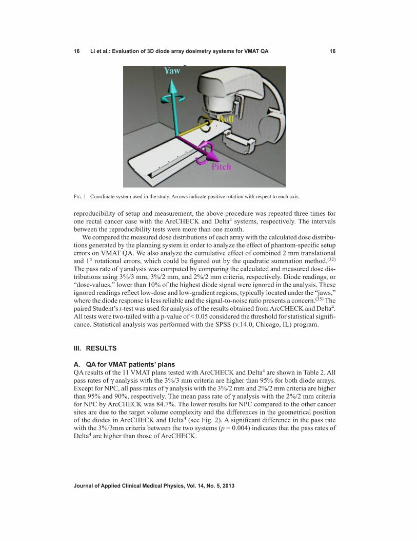
D. Setup error simulationThe ArcCHECK and Delta4 phantoms were translated respectively in the right–left (RL), anterior–posterior (AP), and superior–inferior (SI) directions by ± 1, ± 2, and ± 3 mm and rotated in the pitch, roll, and yaw directions by ± 1° and ± 2° using the 6D treatment couch. Figure 1 shows the definition of pitch, roll, and yaw used in this study. The 11 VMAT plans were separately delivered to the each of the two phantoms for dose verification; in total, 31 measurements (1 without positional error, 18 with translational errors, and 12 with rotational errors) were performed for each patient plan with one dosimetry system. For the combined
Table 1. Patient characteristics and planning states. Using the SIB technique, two or three dose levels are defined for each patient, except for patients with rectal cancer.
Average Field Average Leaf Average Leaf Number of Dose Monitor Width Travel(a) Travel Speed(b)
Disease Site Patients Levels Units (mm) (mm) (mm/s)
Esophageal 3 2 497±108 37±5 579±75 3.8±0.6 Prostate(c) 1 2 1316 51 848 5.4 Cervix uteri 1 2 906 49 818 5.0 Rectal 3 1 1259±136 82±8 610±57 4.2±0.3 NPC(d) 3 3 668±65 26±1 1418±121 4.5±0.3
a Average leaf travel is calculated over all leaves, excluding leaves which remain closed over all treatment.b Average leaf travel speed is average leaf travel divided by delivery time.c The prostate plan is a whole pelvis and prostate boost plan.d The treatment volume for NPC included all sites: primary, upper, and lower neck with a single VMAT plan.
16 Li et al.: Evaluation of 3D diode array dosimetry systems for VMAT QA 16
Journal of Applied Clinical Medical Physics, Vol. 14, No. 5, 2013
reproducibility of setup and measurement, the above procedure was repeated three times for one rectal cancer case with the ArcCHECK and Delta4 systems, respectively. The intervals between the reproducibility tests were more than one month.
We compared the measured dose distributions of each array with the calculated dose distribu-tions generated by the planning system in order to analyze the effect of phantom-specific setup errors on VMAT QA. We also analyze the cumulative effect of combined 2 mm translational and 1° rotational errors, which could be figured out by the quadratic summation method.(32) The pass rate of γ analysis was computed by comparing the calculated and measured dose dis-tributions using 3%/3 mm, 3%/2 mm, and 2%/2 mm criteria, respectively. Diode readings, or “dose-values,” lower than 10% of the highest diode signal were ignored in the analysis. These ignored readings reflect low-dose and low-gradient regions, typically located under the “jaws,” where the diode response is less reliable and the signal-to-noise ratio presents a concern.(35) The paired Student’s t-test was used for analysis of the results obtained from ArcCHECK and Delta4. All tests were two-tailed with a p-value of < 0.05 considered the threshold for statistical signifi-cance. Statistical analysis was performed with the SPSS (v.14.0, Chicago, IL) program.
III. RESULTS
A. QA for VMAT patients’ plansQA results of the 11 VMAT plans tested with ArcCHECK and Delta4 are shown in Table 2. All pass rates of γ analysis with the 3%/3 mm criteria are higher than 95% for both diode arrays. Except for NPC, all pass rates of γ analysis with the 3%/2 mm and 2%/2 mm criteria are higher than 95% and 90%, respectively. The mean pass rate of γ analysis with the 2%/2 mm criteria for NPC by ArcCHECK was 84.7%. The lower results for NPC compared to the other cancer sites are due to the target volume complexity and the differences in the geometrical position of the diodes in ArcCHECK and Delta4 (see Fig. 2). A significant difference in the pass rate with the 3%/3mm criteria between the two systems (p = 0.004) indicates that the pass rates of Delta4 are higher than those of ArcCHECK.
Fig. 1. Coordinate system used in the study. Arrows indicate positive rotation with respect to each axis.

17 Li et al.: Evaluation of 3D diode array dosimetry systems for VMAT QA 17
Journal of Applied Clinical Medical Physics, Vol. 14, No. 5, 2013
B. Sensitivities of two diode arrays to translational setup errorFigure 3 shows the impact of the translational setup error on 11 patient-specific VMAT QA plans. Setup error was separately introduced in the RL, SI, and AP directions, and the impact was measured using ArcCHECK and Delta4. When the translational setup errors are ± 1, ± 2, and ± 3 mm, respectively, the pass rates of γ analysis with the 3%/3 mm criteria decreased by a maximum of 2.5%, 6.4%, and 14.0% for ArcCHECK and 2.5%, 6.9%, and 12.2% for Delta4 in the RL direction; 6.1%, 8.4%, and 13.4% for ArcCHECK and 1.6%, 6.3%, and 14.4% for Delta4 in the SI direction; 2.0%, 4.5%, and 9.5% for ArcCHECK and 1.7%, 5.1%, and 10.5% for Delta4 in the AP direction.
To further test the difference between the two dosimetry systems in sensitivity to setup error, we compared all of their values for the reduction of γ analysis with the 3%/3 mm criteria in each direction. Significant differences in the pass rate of γ analysis in the RL and SI directions (p = 0.019 and < 0.001, respectively) indicate a higher sensitivity of ArcCHECK diodes than Delta4 diodes to translational setup error in both directions; however, only a nominal difference was observed in the AP direction between the two systems (p = 0.074).
Table 2. The QA results of 11 VMAT plans using ArcCHECK and Delta4 phantoms obtained without introducing any setup error.
γ (%)a of ArcCHECK γ (%)a of Delta4
Cancer Site 3%/3 mm 3%/2 mm 2%/2 mm 3%/3 mm 3%/2 mm 2%/2 mm
Esophageal 98.5±0.3 96.8±0.4 91.2±0.7 99.7±0.3 98.2±1.0 95.3±1.7 Prostate 98.7 97.5 92.9 98.6 96.5 90.6 Cervix uteri 98.5 97.2 91.4 99.2 98.0 92.9 Rectal 98.8±0.9 97.2±1.8 93.6±2.4 99.4±0.4 97.8±1.2 95.8±1.0 NPC 95.6±0.8 92.5±0.9 84.7±1.0 98.5±0.5 95.3±1.9 90.1±2.0
a Gamma (γ) results are the percentage of points passing the gamma criterion of 3%/3 mm, 3%/2 mm, and 2%/2 mm, respectively.
Fig. 2. The two systems measured the different section of the dose distribution because of the geometrical position of the diodes. ArcCHECK and Delta4 diodes positioned on the circular line and the crossline, respectively.

18 Li et al.: Evaluation of 3D diode array dosimetry systems for VMAT QA 18
Journal of Applied Clinical Medical Physics, Vol. 14, No. 5, 2013
The tested results also indicated that the pass rate of γ analysis was most affected by transla-tion in the RL and AP directions for NPC and esophageal cancer, but only affected by transla-tion in the SI direction for prostate cancer. For ArcCHECK, the maximum standard deviations (error bars shown in Fig. 3) which were calculated for the three cases of each disease site for each setup error were 4.0%, 3.3%, and 3.1%, respectively, for NPC, esophageal, and rectal cancer; for Delta4 they were 3.8%, 4.5%, and 4.3%. These results indicate that the effects of translational setup errors on VMAT QA are strongly dependent on patient-specific plans in spite of the same disease site.
C. Sensitivities of two diode arrays to rotational setup errorFigure 4 shows the impact of the rotational setup error for 11 patient-specific VMAT QA. Setup error was separately introduced in the pitch, roll, and yaw directions, and the impact was measured using ArcCHECK and Delta4. When the rotational setup errors were ± 1° and ± 2°, respectively, the pass rates of γ analysis with the 3%/3 mm criteria decreased by a maximum of 5.5% and 9.9% for ArcCHECK and 2.5% and 5.0% for Delta4 in the pitch direction; 5.2% and 19.2% for ArcCHECK and 1.8% and 4.9% for Delta4 in the roll direction; and 8.4% and 23.5% for ArcCHECK and 1.7% and 4.9% for Delta4 in the yaw direction. Significant differ-ences between the two systems in all rotation directions (p < 0.001, = 0.001, and < 0.001 in the pitch, roll, and yaw directions, respectively), indicate that the configuration of the ArcCHECK
Fig. 3. The impact of translational setup errors on dosimetric verification of 11 VMAT plans using ArcCHECK and Delta4 phantoms in (a) RL, (b) SI, and (c) AP directions. The simulated translational setup errors are 1, 2, 3, -1, -2, and -3 mm, respectively. The decreased pass rates of γ analysis from the original results are assessed with the 3%/3 mm criteria.

19 Li et al.: Evaluation of 3D diode array dosimetry systems for VMAT QA 19
Journal of Applied Clinical Medical Physics, Vol. 14, No. 5, 2013
system is more sensitive to rotational setup error than the Delta4 system when determining VMAT QA, and emphasize the importance of accurate rotational positioning during measure-ments using ArcCHECK.
From the results gathered by the two systems, we observed the greatest impact on the pass rate of γ analysis with the 3%/3 mm criteria in all directions for NPC and esophageal cancer. For ArcCHECK, the maximum standard deviations (error bars shown in Fig. 4) were 5.8%, 3.4%, and 2.5%, respectively, for NPC, esophageal, and rectal cancer; for Delta4 they were 1.1%, 2.2%, and 1.6%. These results indicate that the effects of the rotational setup errors on VMAT QA are strongly dependent on patient-specific plans in spite of the same disease site.
D. Influence of setup error on the pass rate of γ analysis with various criteriaTable 3 shows the impact of setup errors in translation and rotation on the pass rate of γ analysis with various criteria attained by ArcCHECK and Delta4. Stricter gamma criteria resulted in a greater impact of the setup error on the pass rate of γ analysis. For a translational setup error of 3 mm, the pass rates of γ analysis with the 2%/2 mm criteria decreased by an average of 13.2% ± 5.5% for ArcCHECK and by an average of 14.6% ± 6.7% for Delta4. For the rotational setup error of 2°, the pass rates of γ analysis with the 2%/2 mm criteria decreased by an average of 14.5% ± 6.6% for ArcCHECK and by an average of 7.0% ± 3.7% for Delta4.
Fig. 4. The impact of rotational setup errors on dosimetric verification of 11 VMAT plans using ArcCHECK and Delta4 phantoms in (a) pitch, (b) roll, and (c) yaw directions. The simulated rotational setup errors are 1°, 2°, -1°, and -2°, respec-tively. The decreased pass rates of γ analysis, compared to the original results, are assessed with the 3%/3 mm criteria.

20 Li et al.: Evaluation of 3D diode array dosimetry systems for VMAT QA 20
Journal of Applied Clinical Medical Physics, Vol. 14, No. 5, 2013
E. Combined reproducibility of setup and measurementFigure 5 shows the standard deviation of pass rates with the 3%/3 mm criteria for the reproduc-ibility tests for one rectal cancer case with the ArcCHECK and Delta4 systems, respectively. The mean standard deviations were 0.59% for ArcCHECK and 0.44% for Delta4 for all repro-ducibility tests in this case, and the mean standard deviations for 1, 2, and 3 mm translational setup errors, respectively, were 0.32%, 0.65%, and 0.83% for ArcCHECK and 0.12%, 0.41%, and 0.88% for Delta4; for 1° and 2° rotational setup errors, respectively, they were 0.41% and 0.75% for ArcCheck and 0.29% and 0.54% for Delta4.
Table 3. Translational and rotational setup errors result in a decrease in the pass rate of γ analysis with various criteria on the average and standard deviation.
ArcCHECK Delta4
Setup Error 3%/3 mm 3%/2 mm 2%/2 mm 3%/3 mm 3%/2 mm 2%/2 mm
Translation 1 mm 0.7±1.0 1.4±1.5 2.0±2.0 0.6±0.6 1.6±1.5 2.1±2.2 2 mm 2.8±1.7 5.0±2.9 6.7±3.5 2.3±1.9 5.4±3.3 7.3±4.2 3 mm 6.9±3.3 10.0±4.9 13.2±5.5 6.1±3.8 11.1±5.5 14.6±6.7 Rotation 1° 1.8±1.9 3.7±2.9 4.9±3.7 0.5±0.8 1.5±1.5 2.5±2.6 2° 8.6±4.7 12.1±5.5 14.5±6.6 2.4±1.7 5.0±2.9 7.0±3.7
Fig. 5. The standard deviation of pass rates with the 3%/3 mm criteria for the reproducibility tests for one rectal cancer case with the ArcCHECK and Delta4 systems, respectively. The tests contain all simulated (a) translational and (b) rota-tional setup errors for this case.

21 Li et al.: Evaluation of 3D diode array dosimetry systems for VMAT QA 21
Journal of Applied Clinical Medical Physics, Vol. 14, No. 5, 2013
F. Cumulative effect of both translational and rotational errorFigure 6 shows the cumulative impact of 2 mm translational and 1° rotational setup errors for the 11 patient-specific VMAT QA using ArcCHECK and Delta4, respectively. For ArcCHECK system, the average decreased pass rates of γ analysis with the 3%/3 mm criteria in all direc-tions were 3.4%, 3.1%, 3.3%, 2.9%, and 5.6%, respectively, for esophageal, prostate, cervix uteri, rectal, and nasopharyngeal cancer, and for Delta4 the average decreased pass rates were 2.9%, 3.3%, 1.7%, 1.4%, and 3.0%, respectively.
IV. DISCUSSION
Patient-specific dosimetric verification has been indispensable for IMRT QA. Furthermore, achieving accurate QA results is critical in detecting discrepancies between delivery and plan-ning. The characteristics of Delta4, as reported by Korreman et al.,(36) were determined by comparing consecutive deliveries of the same plan. The results indicated a strong agreement in all cases for the accumulated dose with dose deviations < 1% for all measurement points and cases. Letourneau et al.(27) assessed the combined reproducibility of the ArcCHECK dosimeter system response and the linear accelerator (Elekta Synergy) for VMAT with the repeat delivery of the head and neck plans. The results demonstrated strong performance and stability of both systems. In our study, we tested the combined reproducibility of setup and measurement. The mean standard deviations were 0.59% (0.06%–1.27%) for ArcCHECK and 0.44% (0.06%–1.06%) for Delta4, which shows good reproducibility. However, the results were slightly worse than the reports above because the pass rate altered more significantly as the setup error increased.
Dosimetric verification in the study indicated that the QA of VMAT assessed by both ArcCHECK and Delta4 met therapeutic quality requirements. However, it has been noted that the pass rate of γ analysis for Delta4 was higher than ArcCHECK, referring to the results for zero setup errors (p = 0.004). The reasons for the differences are as follows. First, ArcCHECK and Delta4 dosimetry systems have very different spatial locations of diode detectors. Thus, each system measures a different section of the total dose distribution and samples different dose gradients (see Fig. 2). Compared to Delta4, dose distributions of ArcCHECK are more complex. Moreover, ArcCHECK is more sensitive to the dose delivery errors and the angular discretization effect because of the different diode locations.(37) Second, the dose error nor-malization was different. To establish the percent dose error normalization value, a different method was used for each device, given the different arrangement of the detectors. The Delta4 results were normalized at the isocenter, while the ArcCHECK results were normalized to the
Fig. 6. The cumulative impact of 2 mm translational and 1° rotational errors was evaluated for the pass rate reduction with 3%/3 mm criteria for both ArcCHECK and Delta4 systems. The calculated average and standard deviation of the pass rate reduction contained the translational and rotational errors of combinations in all directions.

22 Li et al.: Evaluation of 3D diode array dosimetry systems for VMAT QA 22
Journal of Applied Clinical Medical Physics, Vol. 14, No. 5, 2013
maximum measured dose in the detector ring. Moreover, the 10% dose cutoff threshold, below which the voxel is excluded from analysis, may not mean the same on the ArcCHECK diode surface as it does on the Delta4 diode planes.(37)
In all tests of the setup error simulation, the two 3D diode arrays exhibited extreme sensitivity to translational and rotational setup errors in all axes for patient-specific QA results of VMAT plans, while exhibiting strong dependence on the patient-specific plan. In general, we have observed an impact of the translational setup error on the QA results of complex VMAT plans and target volumes such as NPC, a cancer contained in the upper and lower neck regions. We have also observed a marked influence of the rotational setup error on the QA results of VMAT plans with long target volumes, such as esophageal cancer. In this paper, we tested three cases for each of the sites of NPC, esophageal, and rectal cancers. Despite the same cancer site amongst case triplets, a difference in sensitivity to setup errors was observed due to the variation of patient-specific plans. Letourneau et al.(27) assessed the sensitivity of the prototype ArcCHECK dosimetry system for phantom setup error after CBCT image-guided setup. Letourneau and colleagues found specifically that the diodes’ sensitivity to setup error in the RL and AP direc-tions were highly plan-dependent; the direction of the steepest dose gradients for a given plan did not necessarily correspond with the direction of the phantom setup.
In addition, the results in Figs. 3 and 4 for both sets of setup errors indicate some differ-ences in the order of 3%–4% reduction rates between the negative and positive setup errors. The differences are mainly due to the following two reasons. Firstly, the residual setup errors up to 0.5 mm and 0.5° were still present when CBCT and HRTC were used. Secondly, plan-specific features along each translational and rotational setup directions were different, such as the dose gradient orientation.
On the other hand, the respective sensitivities to setup error of ArcCHECK and Delta4 were not uniform. Though the diode arrays demonstrated similar sensitivity to translational setup error, ArcCHECK was slightly more sensitive than Delta4 for the gamma criteria 3%/3 mm, likely measuring a section of the dose distribution with more dose gradients. In addition, com-pared to the translational setup error, ArcCHECK diodes were more sensitive to the rotational setup error than Delta4, due to the difference in spatial locations between the two 3D diode arrays. For the same rotational setup error, the diodes of the ArcCHECK system shift a greater distance than those of Delta4.
The AAPM TG-142 report recommended that the tolerance of laser localization was 1.5 mm for IMRT.(32) For both ArcCHECK and Delta4 systems, 1° rotational error could cause an approximate error of 2 mm on the surface of the phantoms. Therefore, the cumulative effect of the combined 2 mm translational and 1° rotational errors was evaluated, and the average pass rates reduction with the 3%/3 mm criteria were 3.8% and 2.4% for ArcCHECK and Delta4 sys-tems, respectively. The cumulative effect for ArcCHECK system was more obvious than Delta4 system mainly due to the higher sensitivity of ArcCHECK to the rotational error. Especially for NPC tests using ArcCHECK, the cumulative effect was quite obvious; thus, the setup of ArcCHECK should be more accurate than the other cancer sites. In addition, because of the difference in the sensitivity between the two systems, their setup accuracy could be different. As shown in Table 3, in order to achieve less than 3% mean pass rate reduction of VMAT plan QA with the 3%/3 mm criteria, a setup accuracy of 2 mm/1° and 2 mm/2° are required for ArcCheck and Delta4 devices, respectively.
V. CONCLUSIONS
In this study, both the ArcCHECK and Delta4 diode arrays showed high sensitivity to setup errors, and sensitivity of both systems is strongly dependent on patient-specific plans. The sen-sitivity of ArcCHECK to the rotational error was higher than that of Delta4. In order to achieve less than 3% mean pass rate reduction of VMAT plan QA with the 3%/3 mm criteria, a setup

23 Li et al.: Evaluation of 3D diode array dosimetry systems for VMAT QA 23
Journal of Applied Clinical Medical Physics, Vol. 14, No. 5, 2013
accuracy of 2 mm/1° and 2 mm/2° is required for ArcCheck and Delta4 devices, respectively. The cumulative effect of the combined 2 mm translational and 1° rotational errors caused 3.8% and 2.4% mean pass rates reduction with 3%/3 mm criteria, respectively, for ArcCHECK and Delta4 systems. For QA of VMAT plans for NPC using the ArcCHECK system, the setup should be more accurate.
ACkNOwLEDgMENTS
Guangjun Li, Sen Bai, and Nianyong Chen contributed equally to this work. The Delta4 dosimetry system was provided by Beijing HGPT Technology & Trade Co. Ltd. This work was partially supported by the National Natural Science Foundation of China (Grant No. 81101697).
REFERENCES
1. Otto K. Volumetric modulated arc therapy: IMRT in a single arc. Med Phys. 2008;35(1):310–17. 2. Verbakel WF, Cuijpers JP, Hoffmans D, Bieker M, Slotman BJ, Senan S. Volumetric intensity-modulated arc
therapy vs. conventional IMRT in head-and-neck cancer: a comparative planning and dosimetric study. Int J Radiat Oncol Biol Phys. 2009;74(1):252–59.
3. Bertelsen A, Hansen CR, Johansen J, Brink C. Single arc volumetric modulated arc therapy of head and neck cancer. Radiother Oncol. 2010;95(2):142–48.
4. Yu C, Li X, Ma L, Chen D, et al. Clinical implementation of intensity-modulated arc therapy. Int J Radiat Oncol Biol Phys. 2002;53(2):453–63.
5. Cao D, Holmes T, Afghan M, Shepard D. Comparison of plan quality provided by intensity-modulated arc therapy and helical tomotherapy. Int J Radiat Oncol Biol Phys. 2007;69(1):240–50.
6. Bedford J, Nordmark Hansen V, McNair H, et al. Treatment of lung cancer using volumetric modulated arc therapy and image guidance: a case study. Acta Oncol. 2008;47(7):1438–43.
7. Verbakel WF, Senan S, Cuijpers JP, Slotman BJ, Lagerwaard FJ. Rapid delivery of stereotactic radiotherapy for peripheral lung tumors using volumetric intensity-modulated arcs. Radiother Oncol. 2009;93(1):122–24.
8. McGrath SD, Matuszak MM, Yan D, Kestin LL, Martinez AA, Grills IS. Volumetric modulated arc therapy for delivery of hypofractionated stereotactic lung radiotherapy: a dosimetric and treatment efficiency analysis. Radiother Oncol. 2010;95(2):153–57.
9. Ma L, Yu C, Earl M, et al. Optimized intensity-modulated arc therapy for prostate cancer treatment. Int J Cancer. 2001;96(6):379–84.
10. Palma D, Vollans E, James K, et al. Volumetric modulated arc therapy for delivery of prostate radiotherapy: comparison with intensity-modulated radiotherapy and three-dimensional conformal radiotherapy. Int J Radiat Oncol Biol Phys. 2008;72(4):996–1001.
11. Wolff D, Stieler F, Welzel G, et al. Volumetric modulated arc therapy (VMAT) vs. serial tomotherapy, step-and-shoot IMRT and 3-D-conformal RT for treatment of prostate cancer. Radiother Oncol. 2009;93(2):226–33.
12. Guckenberger M, Richter A, Krieger T, Wilbert J, Baier K, Flentje M. Is a single arc sufficient in volumetric-modulated arc therapy (VMAT) for complex-shaped target volumes? Radiother Oncol. 2009;93(2):259–65.
13. Duthoy W, De Gersem W, Vergote K, et al. Clinical implementation of intensity-modulated arc therapy (IMAT) for rectal cancer. Int J Radiat Oncol Biol Phys. 2004;60(3):794–806.
14. Cozzi L, Dinshaw KA, Shrivastava SK, et al. A treatment planning study comparing volumetric arc modulation with RapidArc and fixed field IMRT for cervix uteri radiotherapy. Radiother Oncol. 2008;89(2):180–91.
15. Matuszak M, Sui H, Yan D. Potential impact of volumetric modulated arc therapy on the planning and delivery of radiation therapy. Int J Radiat Oncol Biol Phys. 2008;72(1 Suppl):S651.
16. Kuijper IT, Dahele M, Senan S, Verbakel W. Volumetric modulated arc therapy versus conventional intensity modulated radiation therapy for stereotactic spine radiotherapy: a planning study and early clinical data. Radiother Oncol. 2010;94(2):224–28.
17. Clark GM, Popple RA, Young PE, Fiveash JB. Feasibility of single-isocenter volumetric modulated arc radio-surgery for treatment of multiple brain metastases. Int J Radiat Oncol Biol Phys. 2010;76(1):296–302.
18. Bortfeld T, Webb S. Single-arc IMRT? Phys Med Biol. 2009;54(1):N9–N20. 19. Low D, Dempsey J, Venkatesan R, et al. Evaluation of polymer gels and MRI as a 3-D dosimeter for intensity-
modulated radiation therapy. Med Phys. 1999;26(8):1542–51. 20. Vergote K, De Deene Y, Duthoy W, et al. Validation and application of polymer gel dosimetry for the dose veri-
fication of an intensity-modulated arc therapy (IMAT) treatment. Phys Med Biol. 2004;49(2):287–305. 21. Pallotta S, Marrazzo L, Bucciolini M. Design and implementation of a water phantom for IMRT, arc therapy,
and tomotherapy dose distribution measurements. Med Phys. 2007;34(10):3724–31. 22. Jursinic P and Nelms B. A 2-D diode array and analysis software for verification of intensity modulated radiation
therapy delivery. Med Phys. 2003;30(5):870–79. 23. Spezi E, Angelini A, Romani F, Ferri A. Characterization of a 2D ion chamber array for the verification of radio-
therapy treatments. Phys Med Biol. 2005;50(14):3361–73.

24 Li et al.: Evaluation of 3D diode array dosimetry systems for VMAT QA 24
Journal of Applied Clinical Medical Physics, Vol. 14, No. 5, 2013
24. Poppe B, Blechschmidt A, Djouguela A, et al. Two-dimensional ionization chamber arrays for IMRT plan veri-fication. Med Phys. 2006;33(4):1005–15.
25. Jursinic PA, Sharma R, Reuter J. MapCHECK used for rotational IMRT measurements: step-and-shoot, TomoTherapy, RapidArc. Med Phys. 2010;37(6):2837–46.
26. Bush K, Townson R, Zavgorodni S. Monte Carlo simulation of RapidArc radiotherapy delivery. Phys Med Biol. 2008;53(19):N359–N370.
27. Letourneau D, Publicover J, Kozelka J, Moseley DJ, Jaffray DA. Novel dosimetric phantom for quality assurance of volumetric modulated arc therapy. Med Phys. 2009;36(5):1813–21.
28. Bedford J, Lee Y, Wai P, South C, Warrington A. Evaluation of the Delta4 phantom for IMRT and VMAT verifica-tion. Phys Med Biol. 2009;54(9):N167–N176.
29. Sadagopan R, Bencomo J, Martin R, Nilsson G, Matzen T, Balter P. Characterization and clinical evaluation of a novel IMRT quality assurance system. J Appl Clin Med Phys. 2009;10(2):104–19.
30. Bzdusek K, Friberger H, Eriksson K, Hardemark B, Robinson D, Kaus M. Development and evaluation of an efficient approach to volumetric arc therapy planning. Med Phys. 2009;36(6):2328–39.
31. Yan G, Lu B, Kozelka J, Liu C, Li JG. Calibration of a novel four-dimensional diode array. Med Phys. 2010;37(1):108–15.
32. Klein EE, Hanley J, Bayouth J, et al. Task Group 142 report: quality assurance of medical accelerators. Med Phys. 2009;36(9):4197–212.
33. Sharpe MB, Moseley DJ, Purdie TG, Islam M, Siewerdsen J, Jaffray D. The stability of mechanical calibration for a kV cone beam computed tomography system integrated with linear accelerator. Med Phys. 2006;33(1):136–44.
34. Meyer J, Wilbert J, Baier K, et al. Positioning accuracy of cone-beam computed tomography in combination with a HexaPOD robot treatment table. Int J Radiat Oncol Biol Phys. 2007;67(4):1220–28.
35. Basran PS and Woo MK. An analysis of tolerance levels in IMRT quality assurance procedures. Med Phys. 2008;35(6):2300–07.
36. Korreman S, Medin J, Kjaer-Kristoffersen F. Dosimetric verification of RapidArc treatment delivery. Acta Oncol. 2009;48(2):185–91.
37. Feygelman V, Zhang G, Stevens C, Nelms BE. Evaluation of a new VMAT QA device, or the “X” and “O” array geometries. J Appl Clin Med Phys. 2011;12(2):146–68.

a Corresponding author: Sung-Joon Ye, 101 Daehak-ro Jongno-gu, Seoul, Korea, 110-744; phone: (82) (2) 2072 2819; fax: (82) (2) 741 2819; email: [email protected]
Development of real-time motion verification system using in-room optical images for respiratory-gated radiotherapy
Yang-Kyun Park,1,2 Tae-geun Son,3 Hwiyoung Kim,2 Jaegi Lee,4 Wonmo Sung,2 Il Han Kim,1,2 Kunwoo Lee,3 Young-bong Bang,5 and Sung-Joon Ye1,2,4,5a
Department of Radiation Oncology,1 Seoul National University Hospital, Seoul; Interdisciplinary Program in Radiation Applied Life Science,2 Seoul National University, Seoul; Department of Mechanical and Aerospace Engineering,3 Seoul National University, Seoul; Program in Biomedical Radiation Sciences,4 Department of Transdisciplinary Studies, Graduate School of Convergence Science and Technology, Seoul National University, Seoul; Advanced Institutes of Convergence Technology,5 Seoul National University, Suwon, [email protected]
Received 5 October, 2012; accepted 15 April, 2013
Phase-based respiratory-gated radiotherapy relies on the reproducibility of patient breathing during the treatment. To monitor the positional reproducibility of patient breathing against a 4D CT simulation, we developed a real-time motion verification system (RMVS) using an optical tracking technology. The system in the treatment room was integrated with a real-time position management system. To test the system, an anthropomorphic phantom that was mounted on a motion platform moved on a programmed breathing pattern and then underwent a 4D CT simula-tion with RPM. The phase-resolved anterior surface lines were extracted from the 4D CT data to constitute 4D reference lines. In the treatment room, three infrared reflective markers were attached on the superior, middle, and inferior parts of the phantom along with the body midline and then RMVS could track those markers using an optical camera system. The real-time phase information extracted from RPM was delivered to RMVS via in-house network software. Thus, the real-time anterior–posterior positions of the markers were simultaneously compared with the 4D reference lines. The technical feasibility of RMVS was evaluated by repeat-ing the above procedure under several scenarios such as ideal case (with identical motion parameters between simulation and treatment), cycle change, baseline shift, displacement change, and breathing type changes (abdominal or chest breathing). The system capability for operating under irregular breathing was also investigated using real patient data. The evaluation results showed that RMVS has a competence to detect phase-matching errors between patient’s motion during the treatment and 4D CT simulation. Thus, we concluded that RMVS could be used as an online quality assurance tool for phase-based gating treatments.
PACS number: 87.55.Qr
Key words: gated radiotherapy, external marker tracking, quality assurance, 4D CT
I. IntroductIon
Respiration-induced motion has been a significant challenge in radiotherapy for thoracic and abdominal tumors.(1) To manage this motion, the respiratory gating technique was introduced and evaluated in previous studies.(2,3) In this technique, radiation is controlled by a beam delivery
JournAL oF APPLIEd cLInIcAL MEdIcAL PHYSIcS, VoLuME 14, nuMBEr 5, 2013
25 25
26 Park et al.: Real-time motion verification 26
Journal of Applied Clinical Medical Physics, Vol. 14, No. 5, 2013
system within a particular portion of the patient’s breathing cycle (so-called gating window).(4) The tumor motion only within the gating window is taken into account in both treatment plan-ning and delivery processes. Therefore, with this technique tumor margins can be reduced and, thus, tumor dose escalation is enabled without compromising normal tissue sparing.(5)
One widely used gating system with external marker-based monitoring is the real-time posi-tion management (RPM) system (Varian Medical Systems, Palo Alto, CA). Several studies have been performed to evaluate efficacy of RPM.(6,7) The RPM system provides two alternative methods to define the gating window: phase-based gating and amplitude-based gating.(8) It has been reported that amplitude-based gating results in lower residual motion than phase-based gating.(7,9) However, in some institutions, phase-based gating is preferred for two reasons: (1) phase-based gating provides a stable duty cycle, whereas the amplitude-based gating suf-fers from baseline shifts;(3,9) and (2) some specific CT systems correlate images only in terms of the respiration phase.(8,10)
In the RPM phase-based gating technique, the reproducibility of respiratory motion (e.g., displacement according to the respiratory phase) between simulation and treatment fractions is essential. However, in routine clinical practice, the RPM system with a phase-based mode has not provided any solution to quantitatively compare two displacements during the delivery and the CT simulation. The best way to verify the reproducibility of the respiratory motion is to use X-ray imaging,(4) which results in excessive radiation exposure if the acquisitions are performed frequently during treatment.
To verify the reproducibility of the external marker position, several methods using nonin-vasive optical tracking were proposed. Wong et al.(11) used the ExacTrac system (BrainLAB AG, Feldkirchen, Germany) to monitor a patient’s abdominal surface positions during the deep inhalation breath-hold (DIBH) technique. Venkat et al.(12) developed an audiovisual biofeedback system using a single infrared (IR) reflective marker to improve and verify the reproducibility of external marker positions between simulation and treatment. On the other hand, Plathow et al.(13) demonstrated that the correlation between internal tumor motion and external marker motion was highly dependent on the breathing type such as abdominal breathing and thoracic breathing. This finding supported the idea that motion monitoring with a single external marker could not provide sufficient tracking information for tumor motion.(14,15) Therefore, to improve the internal–external correlation, several studies have proposed multiple external marker track-ing(16) or markerless surface monitoring,(17-19) rather than single external marker tracking. For tracking of multiple markers or a patient’s surface, commercial products such as ExacTrac and GateRT (VisionRT, London, UK) are available on the market. However, so far no study has attempted to use 4D CT data as the reference of motion monitoring to check the positional reproducibility of the multiple external markers or patient’s external surface.
This study aimed to develop a quality assurance technique to quantitatively compare a patient’s external surface motion between 4D CT simulation and treatment for RPM phase-based gating. The developed technique involved stereocamera-based optical tracking, surface extrac-tion from 4D CT simulation data, and a phase synchronization method with RPM. Phantom experiments were performed using a programmable respiratory motion platform to evaluate the performance of our system.
II. MAtErIALS And MEtHodS
A. System overviewA schematic illustration of the proposed quality assurance method for RPM phase-based gating is shown in Fig. 1. A conventional RPM-based gating technique uses a single IR camera, an IR reflective marker bock, and a workstation connected to the beam delivery system. In order to acquire real-time images of patient surface motion according to the signals of the RPM system, the developed system consisted of two wall-mounted stereocameras and multiple IR markers

27 Park et al.: Real-time motion verification 27
Journal of Applied Clinical Medical Physics, Vol. 14, No. 5, 2013
on the patient’s anterior surface, and a phase synchronization program (PSP). The motion error calculator (MEC) was programmed to quantitatively compare acquired real-time images of the multiple IR markers with phase-matched reference images extracted from 4D CT simulation data. Details of the developed system are given in the Materials & Methods Sections C, D, E and F below.
B. Anthropomorphic phantom and motion platformsAn anthropomorphic phantom (Alderson Research Laboratories, New York, NY) and two dif-ferent types of motion platform (A and B) were used to evaluate the system. Platform A was composed of an acrylic stage and two linear actuators that were approximately 40 cm apart along the superior–inferior direction. The actuators oscillated the stage between two positions in the anterior–posterior direction. The two oscillation positions and the cycle can be programmed. In normal mode, these two actuators were synchronized to keep the stage horizontal. However, by fixing one actuator in a certain position, the motion platform can also simulate asymmetric motions, such as abdominal and chest breathing. On the other hand, platform B is a fully pro-grammable motion platform which can simulate arbitrary motions in 3D space, such as patient respiratory data. The platform is composed of polycarbonate panels and four stepping motors to simulate 3D tumor and external marker motion. The positional accuracy of the platform had been evaluated by using a high-resolution laser sensor (RF603, RIFTEK, Minsk, Belarus), of which spatial resolution is 0.03 mm and temporal resolution is 0.01 ms. It was determined to be 0.2 mm.(20) In this study, most of the phantom experiments were performed with platform A because of its simplicity in operation and unique feature of asymmetric motions for breathing type change simulations. Platform B was used to evaluate the accuracy of the optical tracking system and to simulate real patient respiratory data.
Fig. 1. A schematic representation for the developed quality assurance method using real-time motion verification system (RMVS).

28 Park et al.: Real-time motion verification 28
Journal of Applied Clinical Medical Physics, Vol. 14, No. 5, 2013
C. Stereocamera system and IR marker trackingAn IR-based stereocamera enabled us to monitor the phantom’s respiratory motion in real time. The system hardware consisted of two charge-coupled device (CCD) cameras (HVR2300C, Hi Vision System, Korea) with universal serial bus (USB) 2.0 interface, 2 IR filters (B+W 092, Schneider-Kreuznach, Bad Kreuznach, Germany), multiple IR light-emitting diodes (LEDs), and a personal computer (PC) with a 2.8 GHz central processing unit (CPU). A custom-fabricated frame housing the cameras, IR filters, and IR LEDs was mounted on the inferior wall of the treatment room. The stereocamera system was calibrated with a checkerboard template and free software (Camera Calibration Toolbox, Imperial College, London, UK). The calibration proce-dures were performed by following Zhang’s method.(21) Three IR reflective markers (Scotchlite 154 TM 3000X, 3M, St. Paul, MN) having a diameter of 6 mm were attached on the phantom surface along the body midline, even though the system can track multiple external markers simultaneously independent of their positions and number. In our previous studies using the same marker tracking method, the tracking accuracy was found to be 0.4 ± 0.4 mm and 0.2 ± 0.4 mm for 3D and vertical direction, respectively.(22,23)
D. Extraction of 4D CT-based reference linesPhase-resolved anterior body midlines were extracted from the 4D CT simulation data and used as vertical displacement references denoted as “4D reference lines”. A workflow to obtain the 4D reference lines is shown in Fig. 2. Ten phase image sets of the phantom were acquired from a 4D CT scanner (Big Bore Brilliance, Philips Medical Systems, Bothell, WA) equipped with the RPM system. The acquired images were transferred to a treatment planning system (Eclipse, Varian Medical Systems, Palo Alto, CA), and external body surfaces were automatically con-toured in the system by using a CT number threshold of -450 HU. These body contours were then exported into DICOM-RT structure (RS) files. Using in-house DICOM processing software, ten sets of anterior surface midlines tagged by unique respiratory phase values were extracted
Fig. 2. A flow chart demonstrating how to generate the 4D reference lines from 4D CT simulation data.

29 Park et al.: Real-time motion verification 29
Journal of Applied Clinical Medical Physics, Vol. 14, No. 5, 2013
from the RS files. The initially generated ten sets of body midlines were linearly interpolated to create 100 sets of data so that each line was assigned integer phase values ranging from 0 to 99. These 100 body midlines were defined as “4D reference lines” in this study. Finally, the complete sets of the 4D reference lines were exported to a text file.
E. Respiratory phase synchronization with RPMIn RPM-phase based gating, beam-on and -off are controlled by the RPM real-time calculated phase information. It has been reported that the real-time calculated phase is error-prone and the retrospective phase calculation using a RPM log file (called “vxp file”) is more accurate.(8) However, despite of its imperfectness, the real-time calculated phase was our choice for the online verification for detecting any errors by monitoring in real time the relationship between phase and displacement. Therefore, to compare current positions of the tracked markers with the reference line at the same phase taken from the 100 sets of 4D reference lines, the phase synchronization program (PSP) was developed to provide this phase information in real time. The PSP was installed on the RPM workstation and operated simultaneously with RPM software version 1.7.5. As the RPM software provided a clock-shaped interface for displaying respiratory phase values, the PSP set the ROI at the center of the “clock” and processed the image of the ROI in real time, as shown in Fig. 3. Finally, the phase value calculated by the software was then transferred to the RMVS through a LAN.
F. Motion error calculatorThe motion error calculator (MEC) is a software module integrated into the RMVS. Three types of input data were required to run the MEC. The first data were the 3D positions of the external markers tracked by the stereocamera system in real time, the second was the 4D reference lines, and the third was the current phase value acquired from the PSP in real time. First, the MEC
Fig. 3. An illustration of the procedure to acquire the respiratory phase value from the RPM workstation. The PSP processed the ROI set on the “phase clock” and transferred the calculated phase value to the RMVS over a network in real time.

30 Park et al.: Real-time motion verification 30
Journal of Applied Clinical Medical Physics, Vol. 14, No. 5, 2013
imports a text file containing the 100 sets of 4D reference lines. Secondly, current 3D position data of the tracked external markers were acquired by the stereocamera system in real time and simultaneously transferred into the MEC. Thirdly, the MEC received the RPM-generated current phase information from PSP and dynamically selected the reference line corresponding to the current phase value. Finally, displacement error between the external marker positions and the reference line was calculated and displayed on an operator’s monitor screen in real time. Even though the stereocamera system can track 3D coordinates of the markers, only the z-axis value was used to calculate errors. The x-axis value was not used because the 4D reference line was assumed to be a body midline having the x-axis value of 0. On the other hand, the y-axis value was used to find the corresponding projected points of the tracked marker on the 4D reference line. The MEC calculated singed and absolute errors, which are given as follows:
Signed error(Δi) = Pi(t)z − z4DCT( (t), Pi(t)y (1)
Absolute error = | Δi | (2)
where i is the marker index, Δ is the signed error for ith marker, Pi(t)y and Pi(t)z are the y and z component of the 3D position of ith marker at time t, respectively. z4DCT is the anterior–posterior position of the 4D reference lines, and ϕ(t) is the integer value of the respiratory phase at time t. The average error for all markers can be defined as an overall error as follows:
(3)
ΔiOverall error (signed) = 1N
N
i = 1Σ
(4)
Overall error (absolute) = 1N
N
i = 1Σ | Δi |
where N is the number of markers. If the motion error of individual markers exceeds a user-defined tolerance, the MEC can display a warning message to the operator.
The proposed point-to-line matching method allowed us to remove the necessity of an exter-nal marker during 4D CT scan. Even though a corresponding projected point on the reference line is not exactly matched with a tracked point (especially when considering deformation of patient surface), the proposed error metrics can provide quantitative error values when there are some problems in positional reproducibility between simulation and treatment.
G. Phantom evaluation
G.1 Evaluation of system accuracy and precisionPrior to the phantom experiments with various motion parameters, the overall accuracy and precision of the system was evaluated. Even though the accuracy of the stereocamera system and platform B had been evaluated in our previous studies, a test experiment with an irregular breathing pattern was performed by using both stereocamera and platform B. Three IR markers on the RANDO phantom (The Phantom Laboratory, Salem, NY) were tracked in this experiment. On the other hand, to evaluate the accuracy of platform A, a test motion with a displacement of 31 mm and a cycle of 3.1 s was simulated with four equidistant markers and solid water slabs (one more marker and flat surface phantom in this initial evaluation). The motion parameters were then compared with the tracking data acquired by the stereocamera system. Using the test motion, the accuracy of RPM and 4D CT was also evaluated for the comparison purpose.

31 Park et al.: Real-time motion verification 31
Journal of Applied Clinical Medical Physics, Vol. 14, No. 5, 2013
Finally, the accuracy of phase synchronization was evaluated by comparing the respiratory phase data of RPM and RMVS to confirm that both systems have the same phase value when the same positional data is given.
G.2 Evaluation of interfractional changes in breathing motionThree IR reflective markers in an interval of 6 cm were attached on the RANDO phantom surface (superior, middle, and inferior markers), and a RPM marker block was placed beside the middle marker. The phantom (mounted on platform A) oscillated regularly according to a reference motion pattern (“normal breathing” hereafter, for convenience) having a displace-ment of 20 mm, and a cycle of 3.1 s for all three markers. The phantom then underwent a 4D CT scan and 4D reference lines were prepared as described in Section D above. In a treatment room, various motion scenarios were simulated to test whether our system could detect the abnormalities when the motion pattern was changed from that of CT simulation. Figure 4 shows the experimental setup in the treatment room. Five different motion scenarios were designed to simulate possible clinical situations. They included ideal (identical motion parameters between CT simulation and treatment), cycle change, baseline shift, displacement change, and breath-ing type change cases. Figure 5 shows the five motion scenarios graphically. In the ideal case, motion errors were expected to be zero. Even in the cycle change scenario, no motion errors were expected because the RPM phase-based system cannot account for any systematic changes in the breathing cycle. In contrast, the baseline shift, displacement change, and breathing type change scenarios were expected to exhibit significant motion errors in our developed system. In total, eight sets of phantom experiments, the parameters of which are listed in Table 1, were performed in the treatment room. Each experiment took 100 s. Mean signed errors (MSEs) and mean absolute errors (MAEs) between external marker positions and 4D reference lines were evaluated for each experiment.
Fig. 4. Experimental setup for system evaluation on a motion phantom. Two types of motion platform were used for the simulations of breathing type changes (platform A) and irregular breathing (platform B).

32 Park et al.: Real-time motion verification 32
Journal of Applied Clinical Medical Physics, Vol. 14, No. 5, 2013
Fig. 5. Five motion scenarios were taken into account in the phantom experiments: (a) ideal, (b) cycle change, (c) baseline shift, (d) displacement change, and (e) breathing type change.
Table 1. Various motion parameters of the phantom experiments.
Experiment Baseline Displacement (mm) Cycle Scenario No. Description (mm) Superior Middle Inferior (s)
Ideal case 1 Ideal case 0 20 20 20 3.1
Cycle change 2 Longer cycle 0 20 20 20 4.7
Baseline shift 3 Offset -5 -5 20 20 20 3.1 4 Offset +5 5 20 20 20 3.1
Smaller Displacement
5 displacement 0 10 10 10 3.1
change 6 Larger 0 40 40 40 3.1 displacement Abdominal Breathing type 7 breathing 0 14.6 20 25.4 3.1 change Chest 8 breathing 0 25.4 20 14.6 3.1
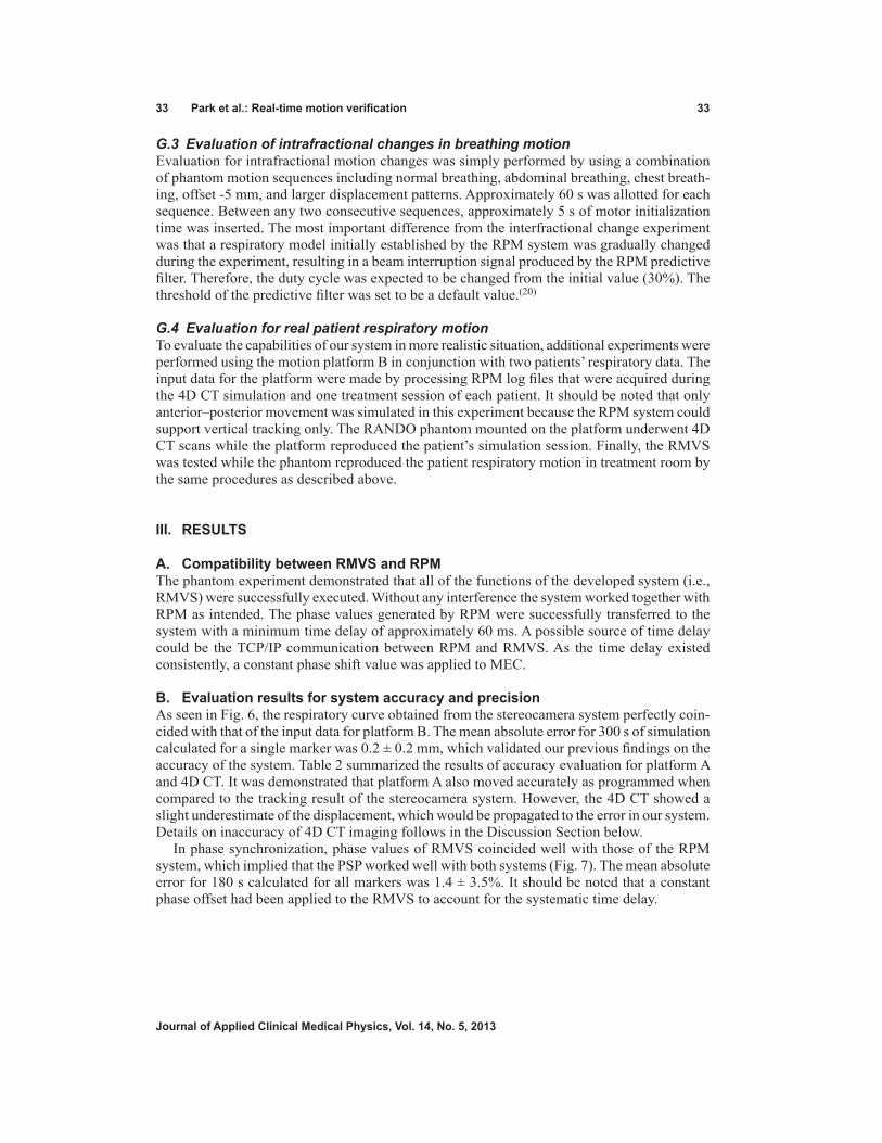
33 Park et al.: Real-time motion verification 33
Journal of Applied Clinical Medical Physics, Vol. 14, No. 5, 2013
G.3 Evaluation of intrafractional changes in breathing motionEvaluation for intrafractional motion changes was simply performed by using a combination of phantom motion sequences including normal breathing, abdominal breathing, chest breath-ing, offset -5 mm, and larger displacement patterns. Approximately 60 s was allotted for each sequence. Between any two consecutive sequences, approximately 5 s of motor initialization time was inserted. The most important difference from the interfractional change experiment was that a respiratory model initially established by the RPM system was gradually changed during the experiment, resulting in a beam interruption signal produced by the RPM predictive filter. Therefore, the duty cycle was expected to be changed from the initial value (30%). The threshold of the predictive filter was set to be a default value.(20)
G.4 Evaluation for real patient respiratory motionTo evaluate the capabilities of our system in more realistic situation, additional experiments were performed using the motion platform B in conjunction with two patients’ respiratory data. The input data for the platform were made by processing RPM log files that were acquired during the 4D CT simulation and one treatment session of each patient. It should be noted that only anterior–posterior movement was simulated in this experiment because the RPM system could support vertical tracking only. The RANDO phantom mounted on the platform underwent 4D CT scans while the platform reproduced the patient’s simulation session. Finally, the RMVS was tested while the phantom reproduced the patient respiratory motion in treatment room by the same procedures as described above.
III. rESuLtS
A. Compatibility between RMVS and RPMThe phantom experiment demonstrated that all of the functions of the developed system (i.e., RMVS) were successfully executed. Without any interference the system worked together with RPM as intended. The phase values generated by RPM were successfully transferred to the system with a minimum time delay of approximately 60 ms. A possible source of time delay could be the TCP/IP communication between RPM and RMVS. As the time delay existed consistently, a constant phase shift value was applied to MEC.
B. Evaluation results for system accuracy and precisionAs seen in Fig. 6, the respiratory curve obtained from the stereocamera system perfectly coin-cided with that of the input data for platform B. The mean absolute error for 300 s of simulation calculated for a single marker was 0.2 ± 0.2 mm, which validated our previous findings on the accuracy of the system. Table 2 summarized the results of accuracy evaluation for platform A and 4D CT. It was demonstrated that platform A also moved accurately as programmed when compared to the tracking result of the stereocamera system. However, the 4D CT showed a slight underestimate of the displacement, which would be propagated to the error in our system. Details on inaccuracy of 4D CT imaging follows in the Discussion Section below.
In phase synchronization, phase values of RMVS coincided well with those of the RPM system, which implied that the PSP worked well with both systems (Fig. 7). The mean absolute error for 180 s calculated for all markers was 1.4 ± 3.5%. It should be noted that a constant phase offset had been applied to the RMVS to account for the systematic time delay.
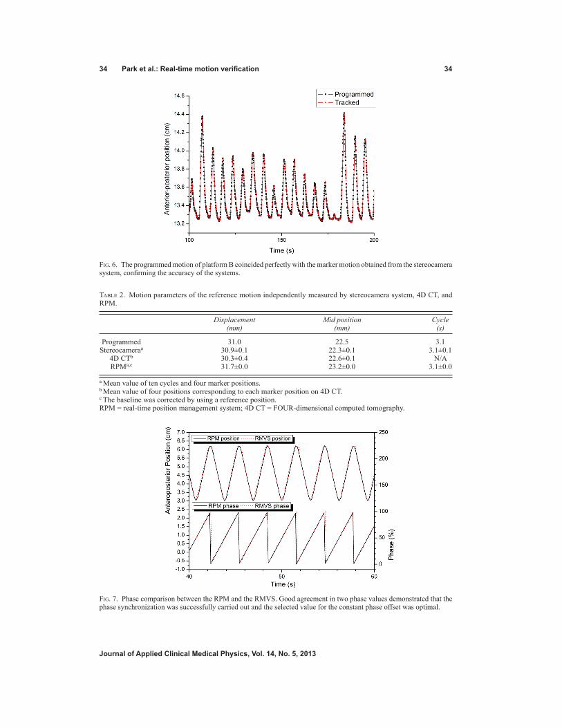
34 Park et al.: Real-time motion verification 34
Journal of Applied Clinical Medical Physics, Vol. 14, No. 5, 2013
Fig. 6. The programmed motion of platform B coincided perfectly with the marker motion obtained from the stereocamera system, confirming the accuracy of the systems.
Fig. 7. Phase comparison between the RPM and the RMVS. Good agreement in two phase values demonstrated that the phase synchronization was successfully carried out and the selected value for the constant phase offset was optimal.
Table 2. Motion parameters of the reference motion independently measured by stereocamera system, 4D CT, and RPM.
Displacement Mid position Cycle (mm) (mm) (s)
Programmed 31.0 22.5 3.1 Stereocameraa 30.9±0.1 22.3±0.1 3.1±0.1 4D CTb 30.3±0.4 22.6±0.1 N/A RPMa,c 31.7±0.0 23.2±0.0 3.1±0.0
a Mean value of ten cycles and four marker positions.b Mean value of four positions corresponding to each marker position on 4D CT.c The baseline was corrected by using a reference position.RPM = real-time position management system; 4D CT = FOUR-dimensional computed tomography.

35 Park et al.: Real-time motion verification 35
Journal of Applied Clinical Medical Physics, Vol. 14, No. 5, 2013
C. Phantom evaluation resultsFigure 8 shows the 4D CT images of the phantom with the normal breathing. For the comparison purpose, 4D CT images from abdominal and chest breathing motions are also illustrated. It was observed that even though the breathing type changed, the movement of the central region of the phantom was similar to that of the reference breathing, which would be a potential pitfall of single marker-based monitoring.
C.1 Evaluation of interfractional changes in breathing motionFrom these experiments, it was confirmed that RPM phase-based gating didn’t provide any warning or interruption signals, even if there were significant interfractional changes in respira-tory motion pattern. This supports the usefulness of our system as a respiratory QA tool. For each experiment, MSEs and MAEs between external marker positions and 4D reference lines were calculated. These are summarized in Tables 3 and 4 and graphically shown in Fig. 9. MSE mode was useful to detect baseline shifts with their direction (overall errors of -5.0 ± 0.9 and 5.1 ± 0.9 mm for experiments 3 and 4, respectively). In MAE mode, the system detected errors even in the ideal and cycle change cases (overall errors of 0.8 ± 0.5, and 0.7 ± 0.5 mm for experiments 1 and 2, respectively), which turned out to be the systematic error in our system. Relatively large errors and deviations were observed in the displacement change experiments compared to the ideal case (overall errors of 2.7 ± 1.2, and 5.9 ± 3.6 for experiments 5, and 6, respectively). For breathing type change cases, the errors of the middle marker were relatively small (0.9 ± 0.7 and 1.5 ± 1.0 for experiment 7 and 8, respectively), compared to those of the inferior and superior markers (inferior marker error of 2.5 ± 1.7 for experiment 7 and superior
Fig. 8. Phantom sagittal images from 4D CT sets acquired during reference motion, abdominal breathing, and chest breathing. The dotted line was set parallel to the middle surface point on the end-of-exhale phase image.

36 Park et al.: Real-time motion verification 36
Journal of Applied Clinical Medical Physics, Vol. 14, No. 5, 2013
marker error of 2.5 ± 1.5 for experiment 8). This result indicated that our multiple marker tracking can detect the abnormal changes in breathing type even when a single marker-based system misses them.
Table 3. MSEs between positions of the tracked makers and the 4D reference lines from the experiment of interfrac-tional motion change.
Experiment MSE ± SD (mm) No. Description Superior Middle Inferior Overall
1 Ideal case 0.1±0.9 0.0±0.9 0.3±0.9 0.1±0.9 2 Longer cycle -0.2±0.9 0.1±0.9 0.0±0.8 0.0±0.9 3 Offset -5 -5.1±0.9 -4.9±0.9 -5.0±0.9 -5.0±0.9 4 Offset +5 5.0±1.0 5.2±0.9 5.1±0.9 5.1±0.9 5 Smaller displacement -0.1±2.9 0.0±2.9 0.1±2.9 0.0±2.9 6 Larger displacement -0.1±6.9 0.2±7.0 0.1±6.9 0.1±6.9 7 Abdominal breathing -0.8±1.4 -0.6±0.9 -0.9±2.9 -0.8±1.9 8 Chest breathing -0.2±2.9 0.4±1.8 0.0±1.4 0.1±2.1
MSE = mean signed error; SD = standard deviation.
Table 4. MAEs between positions of the tracked markers and the 4D reference lines from the experiment of inter-fractional motion change.
Experiment MAE ± SD (mm) No. Description Superior Middle Inferior Overall
1 Ideal case 0.8±0.6 0.8±0.5 0.7±0.5 0.8±0.5 2 Longer cycle 0.7±0.5 0.7±0.5 0.7±0.4 0.7±0.5 3 Offset -5 5.1±0.9 4.9±0.9 5.0±0.9 5.0±0.9 4 Offset +5 5.0±1..0 5.2±0.9 5.1±0.9 5.1±0.9 5 Smaller displacement 2.6±1.2 2.7±1.3 2.7±1.2 2.7±1.2 6 Larger displacement 6.0±3.6 6.0±3.6 5.8±3.7 5.9±3.6 7 Abdominal breathing 1.4±0.8 0.9±0.7 2.5±1.7 1.6±1.4 8 Chest breathing 2.5±1.5 1.5±1.0 1.2±0.6 1.2±0.6
MAE = mean absolute error; SD = standard deviation.
Fig. 9. MAEs between positions of the tracked makers and the 4D reference lines in the phantom experiments. The error bars represent 1 standard deviation.

37 Park et al.: Real-time motion verification 37
Journal of Applied Clinical Medical Physics, Vol. 14, No. 5, 2013
Figure 10 shows the result of overall motion errors separately calculated for four different phases (i.e., end-of-exhale (EOE), inhale, end-of-inhale (EOI), and exhale]. This result dem-onstrated that, for breathing pattern changes related to displacement (experiments 5-8), EOE and EOI are more sensitive to detect such changes than other phases.
C.2 Evaluation of intrafractional changes in breathing motionIn contrast to the interfractional change experiments, the RPM predictive filter in part provided beam-off signals in the gating window for the intrafractional changes in breathing motion. However, after a few cycles, the beam-on signal was resumed. Table 5 summarized duty cycles and motion errors measured during the beam-on time. The results indicated that our system can report on the significant intrafractional motion changes even when the RPM predictive filter cannot fully handle this problem. Figure 11 shows error logs for each marker as a function of the simulation time.
Fig. 10. Motion errors analyzed separately for each respiratory phase (end-of-exhale (EOE), inhale, end-of-inhale (EOI), and exhale). The error bars represent 1 standard deviation.
Table 5. Duty cycle and positional error during beam-on time from the experiment of intrafractional motion changes.
Simulation Time Duty Cycle MAE ± SD (mm) Motion Sequence (s) (%) Superior Middle Inferior Overall
Normal breathing (4D CT reference motion) 53.9 30.3 0.6±0.5 0.7±0.4 0.7±0.4 0.7±0.4
Abdominal breathing 59.5 26.3 0.9±0.6 0.9±0.6 4.4±1.3 2.0±1.9 Chest breathing 57.9 29.7 3.2±1.6 1.5±0.9 1.2±0.7 2.0±2.0 Offset -5 57.0 26.0 5.1±1.3 5.0±1.1 5.1±1.0 5.1±1.1 Larger displacement 57.0 28.4 7.9±2.7 7.9±2.7 7.9±2.7 7.9±2.7
MAE = mean absolute error; SD = standard deviation

38 Park et al.: Real-time motion verification 38
Journal of Applied Clinical Medical Physics, Vol. 14, No. 5, 2013
C.3 Evaluation results for real patient respiratory motionWhile platform B simulated the real patient motion for approximately 300 s, the anterior–posterior positional errors between the tracked markers and the 4D reference lines were suc-cessfully reported by RMVS in real time. Figure 12 demonstrated that patient 1’s breathing was rather irregular, but in a stable baseline. On the other hand, a gradual baseline drift was observed in the simulation of patient 2’s respiratory data, as seen in Fig. 13. Table 6 summarized the evaluation results.
Fig. 11. A motion log with signed errors acquired from the intrafractional change experiment. The breathing motion changes could be detected in real time by monitoring positional errors from multiple marker data.

39 Park et al.: Real-time motion verification 39
Journal of Applied Clinical Medical Physics, Vol. 14, No. 5, 2013
Fig. 12. The tracking result of RMVS for a single marker in the experiment with real patient data (patient 1). Irregularities were observed in tracked marker positions (solid black line). Error events (solid blue line) could be detected in real time by using the reference positions from the 4D CT (dotted red line). A tolerance level was set to ± 3 mm for the example purpose (dotted blue line).
Fig. 13. The tracking result of RMVS for a single marker in the experiment with real patient data (patient 2). A significant baseline shift over time was observed in the tracked marker positions (solid black line). As seen in the error curve (solid blue line), this abnormality could be detected by comparing the marker positions with the reference positions from the 4D CT (dotted red line). A tolerance level was set to ± 3 mm for the example purpose (dotted blue line).
Table 6. MAEs between positions of the tracked markers and the 4D reference lines from the experiments with real patient data.
MAE ± SD (mm)a
Patient EOE Inhalation EOI Exhalation No. (35%–65%) (65%–85%) (85%–5%) (15%–35%) Overall
Patient 1 0.8±0.4 1.1±0.8 1.7±1.2 1.1±0.9 1.2±0.9 Patient 2 1.9±1.4 2.9±1.9 2.2±1.6 1.5±1.1 2.1±1.6a Mean value of all three markers.MAE = mean absolute error; SD = standard deviation; EOE = end of exhalation; EOI = end of inhalation.

40 Park et al.: Real-time motion verification 40
Journal of Applied Clinical Medical Physics, Vol. 14, No. 5, 2013
IV. dIScuSSIon
The assumption of this study was that there would be good correlation between the tumor and the marker movements and that this correlation would be consistent over the entire course of the treatment. Several studies demonstrated good correlation between external marker motion and internal organ movement in free-breathing respiratory gating treatment.(3,24) In contrast, some studies reported significant interfractional variability in the internal–external correlation.(2,25) Similarly, Hoisak et al.(26) found that intrafractional variations in the tumor-surrogate rela-tionship occurred less frequently and with smaller magnitude than interfractional variations, which supported the necessity of once-daily imaging to improve interfractional reproducibility. Therefore, if pretreatment 4D CBCT is available, the developed system together with daily-basis 4D reference positions can be optimally used to evaluate intrafractional error. In such cases the 4D CBCT can be used to correct the interfractional error and to update the baseline of an internal–external correlation function.
Venkat et al.(12) proposed a novel method to improve respiratory reproducibility between simulation and treatment. They created a guiding waveform from the RPM signal during CT simulation, and this waveform was used as a visual biofeedback signal during treatment. However, in their study, quantitative evaluation based on treatment room coordinates was not performed due to the limitation of the RPM calculating the 3D position. In addition, placement error of a single RPM marker block can be a source of uncertainty.(27) Major improvements of our technique from the Venkat study include using treatment room coordinates, employing multiple external markers, and introducing the 4D CT-based reference lines.
In this study, RPM real-time calculated phase data were transferred to our system. To acquire patient’s real-time phase information, RPM needs an interface to transmit real-time respiratory signals to third-party software. However, such a function is not included in the current com-mercial version of RPM. A special cooperation of the manufacturer is a prerequisite to extract real-time phase signal from the RPM system.(12) Santoro et al.(8) reported that the RPM real-time calculated phase data was error-prone and the retrospective phase calculation using a RPM log file (so-called “vxp file”) was more accurate. However, this log file can be exported only after the treatment session, and thus the retrospectively calculated phase data cannot be used for the online quality assurance purpose.
It was noteworthy that in the MAE analysis, the experiment 1 (ideal case) exhibited an inherent systematic error of approximately 1 mm. Although there were several potential sources of this error, such as uncertainties of stereocamera-based tracking, instability of the motion phantom, and so on, it most likely stemmed from the geometric inaccuracy of 4D CT data (as shown in the Results SectionB). Biederer et al.(28) and Hurkmans et al.(29) previously reported that 4D CT scans underestimate the displacement of tumor motion due to their limited temporal resolution. Further study is required to improve the accuracy of the 4D CT.
The results of the phantom experiments indicated that our system could not detect any abnormalities due to the respiratory cycle change alone. The respiratory cycle change leads to a change in transpulmonary pressure, which in turn would potentially cause a change in hysteresis patterns.(4) Since the correlation of organ movement patterns and external surrogate markers is highly dependent on hysteresis patterns, it is inferred that the reproducibility of respiratory cycle is crucial in respiratory gated treatment. It has been reported that an audiovisual biofeedback(9) or audio prompts(30) are effective to help patients to reproduce their planned breathing cycle. We believe that these techniques can be used in conjunction with our system to overcome the limitation related to the respiratory cycle change. The other limitation of our study is the linear interpolation of 4D reference lines at intermediate phases. Future work will address the use of more realistic interpolation methods, such as the B-spline deformable registration model proposed by Schreibmann et al.(31)
In this study, multiple external markers were placed along the body midline, which may raise a question whether the motion of the body midline is representative for that of the entire

41 Park et al.: Real-time motion verification 41
Journal of Applied Clinical Medical Physics, Vol. 14, No. 5, 2013
surface of the abdomen and chest. Recently, Fayad et al.(32) investigated external–internal cor-relation for different ROI positions on the body surface. In their study, it was demonstrated that a central region of the anterior body surface exhibits higher correlation than a lateral region, which justified our approach. Further study is in progress using arbitrarily positioned multiple markers to monitor the entire body surface.
V. concLuSIonS
RPM phase-based gating is vulnerable to interfractional and intrafractional variations in breath-ing motions, which can lead to the geographic miss in radiotherapy. Utilizing 4D CT simulation data and optical tracking of multiple external markers, we have developed a real-time quality assurance tool that can verify the positional reproducibility of patients’ breathing between the simulation and treatments. The phantom experiments demonstrated that our system was fully compatible with RPM and could quantitatively detect real-time positional errors from baseline shifts, displacement changes, breathing motion changes, and irregular breathing. The multiple marker-based tracking also showed a competence to detect errors from breathing motion changes that the single marker-based tracking might miss.
AcknowLEdgMEntS
This work was supported in part by the SNU Brain Fusion Program Research Grant No. 400-20100049 (2010-2011) and the National Research Foundation of Korea (NRF) grant (800-20120109 and 490-20120026) funded by the Korea government (MEST).
rEFErEncES
1. Balter JM, Dawson LA, Kazanjian S, et al. Determination of ventilatory liver movement via radiographic evalu-ation of diaphragm position. Int J Radiat Oncol Biol Phys. 2001;51(1):267–70.
2. Ford EC, Mageras GS, Yorke E, Rosenzweig KE, Wagman R, Ling CC. Evaluation of respiratory movement during gated radiotherapy using film and electronic portal imaging. Int J Radiat Oncol Biol Phys. 2002;52(2):522–31.
3. Mageras GS, Yorke E, Rosenzweig K, et al. Fluoroscopic evaluation of diaphragmatic motion reduction with a respiratory gated radiotherapy system. J Appl Clin Med Phys. 2001;2(4):191–200.
4. Keall PJ, Mageras GS, Balter JM, et al. The management of respiratory motion in radiation oncology report of AAPM Task Group 76. Med Phys. 2006;33(10):3874–900.
5. Wagman R, Yorke E, Ford E, et al. Respiratory gating for liver tumors: use in dose escalation. Int J Radiat Oncol Biol Phys. 2003;55(3):659–68.
6. Berson AM, Emery R, Rodriguez L, et al. Clinical experience using respiratory gated radiation therapy: com-parison of free-breathing and breath-hold techniques. Int J Radiat Oncol Biol Phys. 2004;60(2):419–26.
7. Vedam SS, Keall PJ, Kini VR, Mohan R. Determining parameters for respiration-gated radiotherapy. Med Phys. 2001;28(10):2139–46.
8. Santoro JP, Yorke E, Goodman KA, Mageras GS. From phase-based to displacement-based gating: a software tool to facilitate respiration-gated radiation treatment. J Appl Clin Med Phys. 2009;10(4):2982.
9. George R, Chung TD, Vedam SS, et al. Audio-visual biofeedback for respiratory-gated radiotherapy: impact of audio instruction and audio-visual biofeedback on respiratory-gated radiotherapy. Int J Radiat Oncol Biol Phys. 2006;65(3):924–33.
10. Vedam S, Archambault L, Starkschall G, Mohan R, Beddar S. Determination of prospective displacement-based gate threshold for respiratory-gated radiation delivery from retrospective phase-based gate threshold selected at 4D CT simulation. Med Phys. 2007;34(11):4247–55.
11. Wong VY, Tung SY, Ng AW, Li FA, Leung JO. Real-time monitoring and control on deep inspiration breath-hold for lung cancer radiotherapy—combination of ABC and external marker tracking. Med Phys. 2010;37(9):4673–83.
12. Venkat RB, Sawant A, Suh Y, George R, Keall PJ. Development and preliminary evaluation of a proto-type audiovisual biofeedback device incorporating a patient-specific guiding waveform. Phys Med Biol. 2008;53(11):N197–N208.
13. Plathow C, Zimmermann H, Fink C, et al. Influence of different breathing maneuvers on internal and external organ motion: use of fiducial markers in dynamic MRI. Int J Radiat Oncol Biol Phys. 2005;62(1):238–45.
42 Park et al.: Real-time motion verification 42
Journal of Applied Clinical Medical Physics, Vol. 14, No. 5, 2013
14. Yan H, Zhu G, Yang J, et al. The investigation on the location effect of external markers in respiratory-gated radiotherapy. J Appl Clin Med Phys. 2008;9(2):2758.
15. Killoran JH, Allen AM, Kann BH, Lyatskaya Y. Inter fractional variability of breathing phase definition as deter-mined by fiducial location. Med Phys. 2008;35(2):753–63.
16. Yan H, Yin FF, Zhu GP, Ajlouni M, Kim JH. The correlation evaluation of a tumor tracking system using multiple external markers. Med Phys. 2006;33(11):4073–84.
17. Schaller C, Penne J, Hornegger J. Time-of-flight sensor for respiratory motion gating. Med Phys. 2008;35(7):3090–93.
18. Price GJ, Parkhurst JM, Sharrock PJ, Moore CJ. Real-time optical measurement of the dynamic body surface for use in guided radiotherapy. Phys Med Biol. 2012;57(2):415–36.
19. Wentz T, Fayad H, Bert J, et al. Accuracy of dynamic patient surface monitoring using a time-of-flight camera and B-spline modeling for respiratory motion characterization. Phys Med Biol. 2012;57(13):4175–93.
20. Lee JH. Development of a 4-axis moving platform for simulating respiratory motion in radiotherapy [disserta-tion]. Seoul, Korea: Seoul National University; 2012.
21. Zhang ZY. A flexible new technique for camera calibration. IEEE Pattern Anal Machine. 2000;22(11):1330–34. 22. Kim H, Park YK, Kim IH, Lee K, Ye S-J. Development of an optical-based image guidance system: technique
detecting external markers behind a full facemask. Med Phys. 2011;38(6):3006–12. 23. Park YK, Kim S, Kim H, Kim IIH, Lee K, Ye S-J. Quasi-breath-hold technique using personalized audio-visual
biofeedback for respiratory motion management in radiotherapy. Med Phys. 2011;38(6):3114–24. 24. Beddar A, Kainz K, Briere T, et al. Correlation between internal fiducial tumor motion and external marker motion
for liver tumors imaged with 4D-CT. Int J Radiat Oncol Biol Phys. 2007;67(2):630–38. 25. Tsunashima Y, Sakae T, Shioyama Y, et al. Correlation between the respiratory waveform measured using a respi-
ratory sensor and 3D tumor motion in gated radiotherapy. Int J Radiat Oncol Biol Phys. 2004;60(3):951–58. 26. Hoisak J, Sixel K, Tirona R, Cheung P, Pignol J. Prediction of lung tumour position based on spirometry and on
abdominal displacement: accuracy and reproducibility. Radiother Oncol. 2006;78(3):339–46. 27. Chi PC, Balter P, Luo D, Mohan R, Pan T. Relation of external surface to internal tumor motion studied with cine
CT. Med Phys. 2006;33(9):3116–23. 28. Biederer J, Dinkel J, Remmert G, et al. 4D-Imaging of the lung: reproducibility of lesion size and displace-
ment on helical CT, MRI, and cone beam CT in a ventilated ex vivo system. Int J Radiat Oncol Biol Phys. 2009;73(3):919–26.
29. Hurkmans CW, van Lieshout M, Schuring D, et al. Quality assurance of 4D-CT scan techniques in multicenter phase III trial of surgery versus stereotactic radiotherapy (radiosurgery or surgery for operable early stage (stage 1A) non-small-cell lung cancer [ROSEL] study). Int J Radiat Oncol Biol Phys. 2011;80(3):918–27.
30. Kini VR, Vedam SS, Keall PJ, Patil S, Chen C, Mohan R. Patient training in respiratory-gated radiotherapy. Med Dosim. 2003;28(1):7–11.
31. Schreibmann E, Yang Y, Boyer A, Li T, Xing L. Image interpolation in 4D CT using a BSpline deformable reg-istration model [abstract]. Med Phys. 2005;32(6):1924.
32. Fayad H, Pan T, Clement FJ, Visvikis D. Technical Note: Correlation of respiratory motion between external patient surface and internal anatomical landmarks. Med Phys. 2011;38(6):3157–64.
a Corresponding author: Mitsuhiro Nakamura, Department of Radiation Oncology and Image-applied Therapy, Graduate School of Medicine, Kyoto University, 54 Shogoin-Kawaharacho, Sakyo-ku, Kyoto, 606-8507, Japan; phone: +81-75-751-3762; fax: +81-75-771-9749; email: [email protected]
Effects of interportal error on dose distribution in patients undergoing breath-holding intensity-modulated radiotherapy for pancreatic cancer: evaluation of a new treatment planning method
Toru Takakura,1,2 Mitsuhiro Nakamura,3a Keiko Shibuya,4 Manabu Nakata,1 Akira Nakamura,3 Matsuo Yukinori,3 Takeshi Shiinoki,4 Kyoji Higashimura,1 Teruki Teshima,5 Masahiro Hiraoka3
Clinical Radiology Service Division,1 Kyoto University Hospital, Kyoto; Department of Medical Physics and Engineering,2 Graduate School of Medicine, Osaka University, Osaka; Department of Radiation Oncology and Image-applied Therapy,3 Graduate School of Medicine, Kyoto University, Kyoto; Department of Therapeutic Radiology,4 Graduate School of Medicine, Yamaguchi University, Yamaguchi; Department of Radiation Oncology,5 Osaka Medical Center for Cancer and Cardiovascular Diseases, Osaka, Japan [email protected]
Received 20 December, 2012; accepted 23 May 2013
In patients with pancreatic cancer, intensity-modulated radiotherapy (IMRT) under breath holding facilitates concentration of the radiation dose in the tumor, while sparing the neighboring organs at risk and minimizing interplay effects between movement of the multileaf collimator and motion of the internal structures. Although the breath-holding technique provides high interportal reproducibility of target posi-tion, dosimetric errors caused by interportal breath-holding positional error have not been reported. Here, we investigated the effects of interportal breath-holding positional errors on IMRT dose distribution by incorporating interportal positional error into the original treatment plan, using random numbers in ten patients treated for pancreatic cancer. We also developed a treatment planning technique that short-ens breath-holding time without increasing dosimetric quality assurance workload. The key feature of our proposed method is performance of dose calculation using the same optimized fluence map as the original plan, after dose per fraction in the original plan was cut in half and the number of fractions was doubled. Results confirmed that interportal error had a negligible effect on dose distribution over multiple fractions. Variations in the homogeneity index and the dose delivered to 98%, 2%, and 50% of the volume for the planning target volume, and the dose delivered to 1 cc of the volume for the duodenum and stomach were ± 1%, on average, in comparison with the original plan. The new treatment planning method decreased breath-holding time by 33%, and differences in dose-volume metrics between the original and the new treatment plans were within ± 1%. An additional advantage of our proposed method is that interportal errors can be better averaged out; thus, dose distribution in the proposed method may be closer to the planned dose distribution than with the original plans.
PACS number: 87.53.Bn, 87.55.D-, 87.55.-x
Key words: IMRT, pancreas cancer, breath-holding technique
JOURNAL OF APPLIED CLINICAL MEDICAL PHYSICS, VOLUME 14, NUMBER 5, 2013
43 43

44 Takakura et al.: Effect of interportal error on dose distribution in breath-holding IMRT 44
Journal of Applied Clinical Medical Physics, Vol. 14, No. 5, 2013
I. INTRODUCTION
Pancreatic cancer is currently the fifth-leading cause of death from cancer in Japan.(1) The number of people dying from this cancer has increased annually, and reached approxi-mately 28,000 deaths in 2010. Although the first-choice curative treatment for pancreatic cancer remains surgery, more than 80% of patients have nonresectable disease at the time of diagnosis.(2) These cases are often treated with chemoradiotherapy, but the presence of radiosensitive organs at risk (OARs) around the pancreas, including the duodenum and stomach, prevents the delivery of a sufficient radiation dose, which may result in unfavorable outcomes.(3-9) Thus, an important issue in the treatment of pancreatic cancer generally is how to deliver a more intense radiation dose.
Intensity-modulated radiotherapy (IMRT) facilitates the concentration of radiation dose in the tumor, while sparing doses to OARs, and can therefore reduce the rate of gastrointestinal toxicity.(10-12) Respiratory motion remains an obstacle to dose delivery, however, and pancre-atic tumor motion has been confirmed to be greater than 10 mm using several modalities.(13) When respiratory motion is not managed, a larger internal margin is required to fully cover geometric changes in free breathing,(14) which, in turn, results in the incorporation of a large volume of OARs into the planning target volume (PTV) and the possibility of severe gastroin-testinal toxicity.(15) Additionally, the dosimetric advantage of IMRT is degraded significantly by interplay between movement of the multileaf collimator (MLC) and motion of the internal structures,(16-18) resulting in unintended underdose to the tumor and/or overdose to normal tis-sues. These problems seriously hamper the widespread adoption of IMRT for moving tumors, and accordingly indicate the need for respiratory management.
Our department is currently conducting a phase I/II radiation dose escalation study of full-dose gemcitabine with IMRT in pancreatic cancer patients under end-exhalation breath-holding (EE-BH) conditions with a visual-feedback technique (BH-IMRT).(16-18) The goal is to evaluate the possible impact of our protocol on response, toxicity, pain relief, and outcome in patients with locally advanced nonresectable pancreatic cancer, with reference to previous dose escala-tion trials of full-dose gemcitabine with conventional RT at the University of Michigan.(9,19) We reported previously that the EE-BH technique provided high interportal reproducibility of target position in pancreatic cancer.(20) However, the effects of interportal BH positional error on dosimetric errors have not been reported before. Our previous study also showed that a minimum BH time of 15 sec was required at the lowest dose level (2.6 Gy per fraction) at a dose rate of 600 monitor units (MU)/min. MUs per port were increased at the higher pre-scription dose levels in dose-escalation studies. A long BH time of > 15 sec at EE is typically not only difficult even for healthy people, but also has the potential to cause dosimetric error between the planned and delivered dose distribution as a result of baseline drift.(21) Generally, MUs per port can be reduced in multiport plans having different gantry and couch angles, but dosimetric quality assurance (DQA) of multiport plans requires measurement of each port and is, thus, laborious and time consuming.
The purpose of the present study was to investigate the effects of interportal BH positional errors on dose distribution, and to propose a treatment planning technique that both reduces the effect of interportal BH positional errors and shortens BH time without increasing DQA workload.
II. MATERIALS AND METHODS
This study was conducted in ten patients who underwent BH-IMRT for pancreatic cancer at Kyoto University Hospital between May 2010 and June 2011. Clinical target volume (CTV) and OARs, including duodenum, stomach, kidney, liver, spleen, and spinal cord, were delin-eated manually by a single radiation oncologist to eliminate interobserver variation. A PTV was created by adding isotropic margins of 5 mm to the CTV. The dynamic IMRT plan was
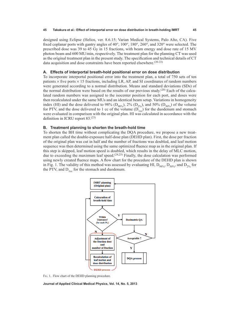
45 Takakura et al.: Effect of interportal error on dose distribution in breath-holding IMRT 45
Journal of Applied Clinical Medical Physics, Vol. 14, No. 5, 2013
designed using Eclipse (Helios, ver. 8.6.15; Varian Medical Systems, Palo Alto, CA). Five fixed coplanar ports with gantry angles of 40°, 100°, 180°, 260°, and 320° were selected. The prescribed dose was 39 to 45 Gy in 15 fractions, with beam energy and dose rate of 15 MV photon beam and 600 MU/min, respectively. The treatment plan for the planning CT was used as the original treatment plan in the present study. The specification and technical details of CT data acquisition and dose constraints have been reported elsewhere.(20-22)
A. Effects of interportal breath-hold positional error on dose distributionTo incorporate interportal positional error into the treatment plan, a total of 750 sets of ten patients × five ports × 15 fractions, including LR, AP, and SI coordinates of random numbers were generated according to a normal distribution. Means and standard deviations (SDs) of the normal distribution were based on the results of our previous study.(20) Each of the calcu-lated random numbers was assigned to the isocenter position for each port, and doses were then recalculated under the same MUs and an identical beam setup. Variations in homogeneity index (HI) and the dose delivered to 98% (D98%), 2% (D2%), and 50% (D50%) of the volume for PTV, and the dose delivered to 1 cc of the volume (D1cc) for the duodenum and stomach were evaluated in comparison with the original plan. HI was calculated in accordance with the definition in ICRU report 83.(23)
B. Treatment planning to shorten the breath-hold timeTo shorten the BH time without complicating the DQA procedure, we propose a new treat-ment plan called the double-exposure half-dose plan (DEHD plan). First, the dose per fraction of the original plan was cut in half and the number of fractions was doubled, and leaf motion sequence was then determined using the same optimized fluence map as in the original plan. If this step is skipped, leaf motion speed is doubled, which results in the delay of MLC motion, due to exceeding the maximum leaf speed.(24,25) Finally, the dose calculation was performed using newly created fluence maps. A flow chart for the procedure of the DEHD plan is shown in Fig. 1. The validity of this method was assessed by evaluating HI, D98%, D50%, and D2% for the PTV, and D1cc for the stomach and duodenum.
Fig. 1. Flow chart of the DEHD planning procedure.

46 Takakura et al.: Effect of interportal error on dose distribution in breath-holding IMRT 46
Journal of Applied Clinical Medical Physics, Vol. 14, No. 5, 2013
C. Comparison of calculated dose fluence mapsTo verify the DEHD plan, the dose distributions for each port in the DEHD plan were calculated on a plane perpendicular to the radiation field at a depth of 10 cm with a virtual phantom on Eclipse, and were then compared with those in the original plan using commercially available radiation dosimetry software (DD system, ver. 9.4; R-Tech Inc., Tokyo, Japan). The dose dis-tribution in the DEHD plan was registered with that in the original plan, based on the isocenter. Dose distribution was not normalized, but was compared for the area receiving more than 50% of the isodose to evaluate the dose around the target using the dose difference criteria of 0.5%, 1.0%, and 2.0%, with a dose grid resolution of 0.39 mm.
III. RESULTS & DISCUSSION
A. Effects of interportal breath-hold positional error on dose distributionFrequency histograms of generated random numbers are shown in Fig. 2. Means ± SDs of random numbers were 0.07 ± 1.12 mm (range, -3.62 to 3.59 mm), 0.12 ± 0.99 mm (range, -2.47 to 3.54 mm), and 0.12 ± 1.26 mm (range, -2.95 to 5.33 mm) in LR, SI, and AP directions, respectively. These values were comparable to those reported previously.(21)
Variations in HI, D98%, D50%, and D2% for the PTV and D1cc for the stomach and duodenum are summarized in Table 1. The data in the third, fourth, and fifth columns are means ± SDs of dose volume metrics from ten patients in the original treatment plan, those from 150 fractions incorporating interportal positional error, and those from averaged sums of 15 fractions for each patient, respectively. The PTV was well-covered by the planned dose, while D1cc for the stomach and duodenum varied interfractionally; however, these variations were small compared
(a) (b)
(c)
Fig. 2. Histograms of error values generated using random numbers in the (a) LR, (b) AP, and (c) SI directions.
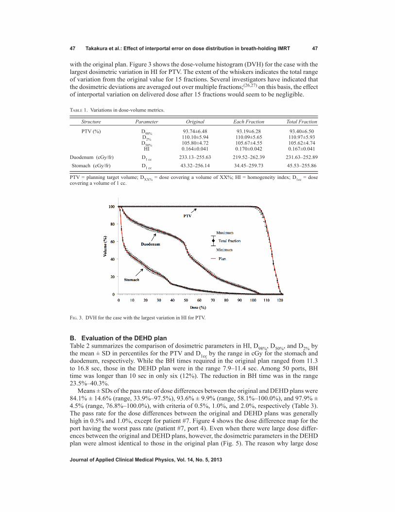
47 Takakura et al.: Effect of interportal error on dose distribution in breath-holding IMRT 47
Journal of Applied Clinical Medical Physics, Vol. 14, No. 5, 2013
with the original plan. Figure 3 shows the dose-volume histogram (DVH) for the case with the largest dosimetric variation in HI for PTV. The extent of the whiskers indicates the total range of variation from the original value for 15 fractions. Several investigators have indicated that the dosimetric deviations are averaged out over multiple fractions;(26,27) on this basis, the effect of interportal variation on delivered dose after 15 fractions would seem to be negligible.
B. Evaluation of the DEHD planTable 2 summarizes the comparison of dosimetric parameters in HI, D98%, D50%, and D2% by the mean ± SD in percentiles for the PTV and D1cc by the range in cGy for the stomach and duodenum, respectively. While the BH times required in the original plan ranged from 11.3 to 16.8 sec, those in the DEHD plan were in the range 7.9–11.4 sec. Among 50 ports, BH time was longer than 10 sec in only six (12%). The reduction in BH time was in the range 23.5%–40.3%.
Means ± SDs of the pass rate of dose differences between the original and DEHD plans were 84.1% ± 14.6% (range, 33.9%–97.5%), 93.6% ± 9.9% (range, 58.1%–100.0%), and 97.9% ± 4.5% (range, 76.8%–100.0%), with criteria of 0.5%, 1.0%, and 2.0%, respectively (Table 3). The pass rate for the dose differences between the original and DEHD plans was generally high in 0.5% and 1.0%, except for patient #7. Figure 4 shows the dose difference map for the port having the worst pass rate (patient #7, port 4). Even when there were large dose differ-ences between the original and DEHD plans, however, the dosimetric parameters in the DEHD plan were almost identical to those in the original plan (Fig. 5). The reason why large dose
Table 1. Variations in dose-volume metrics.
Structure Parameter Original Each Fraction Total Fraction
PTV (%) D98% 93.74±6.48 93.19±6.28 93.40±6.50 D2% 110.10±5.94 110.09±5.65 110.97±5.93 D50% 105.80±4.72 105.67±4.55 105.62±4.74 HI 0.164±0.041 0.170±0.042 0.167±0.041 Duodenum (cGy/fr) D1 cc 233.13–255.63 219.52–262.39 231.63–252.89 Stomach (cGy/fr) D1 cc 43.32–256.14 34.45–259.73 45.53–255.86
PTV = planning target volume; DXX% = dose covering a volume of XX%; HI = homogeneity index; D1cc = dose covering a volume of 1 cc.
Fig. 3. DVH for the case with the largest variation in HI for PTV.

48 Takakura et al.: Effect of interportal error on dose distribution in breath-holding IMRT 48
Journal of Applied Clinical Medical Physics, Vol. 14, No. 5, 2013
differences were observed may be that the MLC control points increased in the DEHD plan when recalculating the leaf motion and actual fluence map. Compared with other ports (31.1% on average), a marked increase in the MLC control points was observed for port 4 in patient #7 (39.8%), which may have caused the relatively large dose difference in actual fluence between the original and DEHD plan. In DMLC IMRT, breath-holding time was not prolonged, even when the MLC control points were increased.
The DEHD plan was capable of reducing BH time by 33%, on average, without markedly reducing the dose-volume parameters in the original plan, facilitating the treatment of patients who find prolonged BH difficult. However, this method increases the frequency of breath hold-ing and prolongs the time the patient is required to maintain the same posture. Accordingly, it is desirable to use the DEHD plan only when difficulties in breath-hold time are expected, or large dosimetric errors in the patient’s body are predicted due to poor reproducibility of the breath-holding position. Selection of the plan in consideration of these advantages and disadvantages can reduce the physical distress in patients and deviations of the actual dose distribution from that calculated in the treatment plan. When the number of ports increased from the original plan, BH time was shortened, but dose-volume metrics and dose distributions were sometimes different from the original plan. The DEHD plan uses the optimized fluence map of the origi-nal plan; thus, further optimization processes are not needed once dose-volume constraints in the original plan are satisfied, while radiation oncologists using the DEHD plan must verify dose-volume metrics and dose distributions. Additionally, medical physicists must check the machine condition and parameters in the radiation treatment planning system and perform additional DQA if there are large differences between the calculated and measured doses. An additional advantage of our proposed method is that interportal BH positional errors can be better averaged out. The dose distribution in the DEHD plan can thus be closer to the planned dose distribution than with the original plan.
Table 2. Comparison of dose-volume metrics between the original and DEHD plans.
Structure Parameter Original DEHD
PTV (%) D98% 93.74±6.48 93.50±6.57 D2% 110.10±5.94 110.96±6.00 D50% 105.80±4.72 105.58±4.77 HI 0.164±0.041 0.165±0.042 Duodenum (cGy/fr) D1 cc 233.13–255.63 233.30–254.10 Stomach (cGy/fr) D1 cc 43.32–256.14 44.30–255.64
PTV = planning target volume; DXX% = dose covering a volume of XX%; HI = homogeneity index; D1cc = dose covering a volume of 1 cc.
Table 3. Pass rate of dose differences between the original and DEHD plans for each patient.
Threshold Pt. 1 Pt. 2 Pt. 3 Pt. 4 Pt. 5 Pt. 6 Pt. 7 Pt. 8 Pt. 9 Pt. 10
0.5% Mean (%) 83.1 95.4 86.9 88.3 86.3 87.3 52.0 80.6 90.2 91.0 SD (%) 2.5 1.4 6.0 5.5 9.4 8.7 20.1 15.8 5.4 6.0 1.0% Mean (%) 93.8 99.6 94.4 98.8 94.7 97.2 74.2 88.4 97.0 97.9 SD (%) 2.9 0.4 4.0 2.2 6.5 3.2 17.1 13.3 1.8 2.6 2.0% Mean (%) 98.4 100.0 97.3 100.0 98.1 99.9 92.7 93.7 99.4 99.9 SD (%) 2.0 0.0 1.8 0.1 2.1 0.1 8.0 9.6 0.8 0.3
SD = standard deviation.

49 Takakura et al.: Effect of interportal error on dose distribution in breath-holding IMRT 49
Journal of Applied Clinical Medical Physics, Vol. 14, No. 5, 2013
Fig. 4. Comparison of dose-difference maps between the original and DEHD plans for the case with the worst pass rate. The red areas indicate failure, with criteria of (a) 0.5%, (b) 1.0%, and (c) 2.0% for the area receiving more than 50% of the dose. The isodose lines displayed in the interval 10% are from the 10% to the 90% isodose lines.

50 Takakura et al.: Effect of interportal error on dose distribution in breath-holding IMRT 50
Journal of Applied Clinical Medical Physics, Vol. 14, No. 5, 2013
IV. CONCLUSIONS
We demonstrated that the effects of interportal error on dose distribution in BH-IMRT are neg-ligible. Additionally, we propose a new method of treatment planning, called the “DEHD plan”. The DEHD plan can shorten BH time without substantially reducing dose-volume metrics and without increasing DQA workload, compared with that required for a multiport plan, because only one of the two identical beams is measured. Finally, the effects of interportal error on dose distribution can be reduced through using the DEHD plan.
ACkNOwLEDgMENTS
This work was supported by a Grant-in-Aid for the Encouragement of Scientists from the Ministry of Education, Culture, Sports, Science and Technology, Japan (Grant No. 23931024), and a Grant-in-Aid for Young Scientists (B) from the Ministry of Education, Culture, Sports, Science and Technology, Japan (Grant No. 23791408).
REFERENCES
1. Cancer Statistics in Japan 2011 [internet]. Tokyo: National Cancer Center of Japan, 2012 [cited 2012 Sep 6]. Available from: http://ganjoho.jp/data/professional/statistics/backnumber/2012/fig01.pdf
2. Warshaw AL and Fernandez-del Castillo C. Medical progress: pancreatic carcinoma. N Engl J Med. 1992;326(7):455–65.
3. Moertel CG, Childs DS Jr, Reitemeier RJ, Colby MY Jr, Holbrook MA. Combined 5-fluorouracil and supervolt-age radiation therapy of locally unresectable gastrointestinal cancer. Lancet. 1969;2(7626):865–67.
4. Moertel CG, Frytak S, Hahn RG, et al. Therapy of locally unresectable pancreatic carcinoma: a randomized comparison of high dose (6000 rads) radiation alone, moderate dose radiation (4000 rads + 5-fluorouracil), and high dose radiation + 5-fluorouracil: The Gastrointestinal Tumor Study Group. Cancer. 1981;48(8):1705–10.
5. Klaassen DJ, MacIntyre JM, Catton GE, Engstrom PF, Moertel CG. Treatment of locally unresectable cancer of the stomach and pancreas: a randomized comparison of 5-fluorouracil alone with radiation plus concurrent and maintenance 5-fluorouracil – an Eastern Cooperative Oncology Group study. J Clin Oncol. 1985;3(3):373–78.
6. Manuyakorn A, Paulus R, Farrell J, et al. Cellular histone modification patterns predict prognosis and treatment response in resectable pancreatic adenocarcinoma: results from RTOG 9704. J Clin Oncol. 2010;28(8):1358–65.
7. Cardenes HR, Moore AM, Johnson CS, et al. A phase II study of gemcitabine in combination with radiation therapy in patients with localized, unresectable, pancreatic cancer: a Hoosier Oncology Group study. Am J Clin Oncol. 2011;34(5):460–65.
Fig. 5. DVH of the original and DEHD plans for patient #7.

51 Takakura et al.: Effect of interportal error on dose distribution in breath-holding IMRT 51
Journal of Applied Clinical Medical Physics, Vol. 14, No. 5, 2013
8. Showalter TN, Winter KA, Berger AC, et al. The influence of total nodes examined, number of positive nodes, and lymph node ratio on survival after surgical resection and adjuvant chemoradiation for pancreatic cancer: a secondary analysis of RTOG 9704. Int J Radiat Oncol Biol Phys. 2011;81(5):1328–35.
9. Allen AM, Zalupski MM, Robertson JM, et al. Adjuvant therapy in pancreatic cancer: Phase I trial of radiation dose escalation with concurrent full-dose gemcitabine. Int J Radiat Oncol Biol Phys. 2004;59(5):1461–67.
10. Ben-Josef E, Shields AF, Vaishampayan U, et al. Intensity-modulated radiotherapy (IMRT) and concurrent capecitabine for pancreatic cancer. Int J Radiat Oncol Biol Phys. 2004;59(2):454–59.
11. Yovino S, Poppe M, Jabbour S, et al. Intensity-modulated radiation therapy significantly improves acute gastro-intestinal toxicity in pancreatic and ampullary cancers. Int J Radiat Oncol Biol Phys. 2011;79(1):158–62.
12. Milano MT, Chmura SJ, Garofalo MC, et al. Intensity-modulated radiotherapy in treatment of pancreatic and bile duct malignancies: toxicity and clinical outcome. Int J Radiat Oncol Biol Phys. 2004;59(2):445–53.
13. Keall PJ, Mageras GS, Balter JM, et al. The management of respiratory motion in radiation oncology report of AAPM Task Group 76. Med Phys. 2006;33(10):3874–900.
14. Mori S, Hara R, Yanagi T, et al. Four-dimensional measurement of intrafractional respiratory motion of pancreatic tumors using a 256 multi-slice CT scanner. Radiother Oncol. 2009;92(2):231–37.
15. Murphy JD, Adusumilli S, Griffith KA, et al. Full-dose gemcitabine and concurrent radiotherapy for unresectable pancreatic cancer. Int J Radiat Oncol Biol Phys. 2007;68(3):801–08.
16. Seco J, Sharp GC, Turcotte J, Gierga D, Bortfeld T, Paganetti H. Effects of organ motion on IMRT treatments with segments of few monitor units. Med Phys. 2007;34(3):923–34.
17. Bortfeld T, Jokivarsi K, Goitein M, Kung J, Jiang SB. Effects of intra-fraction motion on IMRT dose delivery: statistical analysis and simulation. Phys Med Biol. 2002;47(13):2203–20.
18. Chui CS, Yorke E, Hong L. The effects of intra-fraction organ motion on the delivery of intensity-modulated field with a multileaf collimator. Med Phys. 2003;30(7):1736–46.
19. McGinn CJ, Zalupski MM, Shureiqi I, et al. Phase I trial of radiation dose escalation with concurrent weekly full-dose gemcitabine in patients with advanced pancreatic cancer. J Clin Oncol. 2001;19(22):4202–08.
20. Nakamura M, Shibuya K, Shiinoki T, et al. Positional reproducibility of pancreatic tumors under end-exhalation breath-hold conditions using a visual feedback technique. Int J Radiat Oncol Biol Phys. 2011;79(5):1565–71.
21. Nakamura M, Shibuya K, Nakamura A, et al. Interfractional dose variations in intensity-modulated radiotherapy with breath-hold for pancreatic cancer. Int J Radiat Oncol Biol Phys. 2012;82(5):1619–26.
22. Nakamura M, Kishimoto S, Iwamura K, et al. Dosimetric investigation of breath-hold intensity-modulated radiotherapy for pancreatic cancer. Med Phys. 2012;39(1):48–54.
23. ICRU. Special considerations regarding absorbed-dose and dose–volume prescribing and reporting in IMRT. ICRU Report 83. J ICRU. 2010;10(1):27–40.
24. Okumura M, Obata Y, Shimomura K, Tamura M, Nishimura Y. The effect of gantry and collimator angles on leaf limited velocity and position in dynamic multileaf collimator intensity-modulated radiation therapy. Phys Med Biol. 2010;55(11):3101–13.
25. LoSasso T, Chui CS, Ling CC. Comprehensive quality assurance for the delivery of intensity modulated radio-therapy with a multileaf collimator used in the dynamic mode. Med Phys. 2001;28(11):2209–19.
26. Jiang SB, Boyer AL, Ma CM. Modeling the extrafocal radiation and monitor chamber backscatter for photon beam dose calculation. Med Phys. 2001;28(1):55–66.
27. Berbeco RI, Pope CJ, Jiang SB. Measurement of the interplay effect in lung IMRT treatment using EDR2 films. J Appl Clin Med Phys. 2006;7(4):33–42.
a Corresponding author: Marziyeh Behmadi, Medical Physics Department, Faculty of Medicine, Mashhad University of Medical Sciences, Pardis-e-Daneshgah, Vakil Abad Blvd., Azadi Square, Mashhad, Iran 9177948564; phone: +98 511 8002316; fax: +98 511 8002320; email: [email protected]
A Monte Carlo study on electron and neutron contamination caused by the presence of hip prosthesis in photon mode of a 15 MV Siemens PRIMUS linac
Mohammad Taghi Bahreyni Toossi,¹ Marziyeh Behmadi,2a Mahdi Ghorbani,1 Hamid Gholamhosseinian2
Medical Physics Research Center,1 Medical Physics Department, Faculty of Medicine, Mashhad University of Medical Sciences, Mashhad, Iran; Medical Physics Department,2 Faculty of Medicine, Mashhad University of Medical Sciences, Mashhad, [email protected]
Received 11 October, 2012; accepted 28 May, 2013
Several investigators have pointed out that electron and neutron contamination from high-energy photon beams are clinically important. The aim of this study is to assess electron and neutron contamination production by various prostheses in a high-energy photon beam of a medical linac. A 15 MV Siemens PRIMUS linac was simulated by MCNPX Monte Carlo (MC) code and the results of percentage depth dose (PDD) and dose profile values were compared with the measured data. Electron and neutron contaminations were calculated on the beam’s central axis for Co-Cr-Mo, stainless steel, Ti-alloy, and Ti hip prostheses through MC simula-tions. Dose increase factor (DIF) was calculated as the ratio of electron (neutron) dose at a point for 10 × 10 cm² field size in presence of prosthesis to that at the same point in absence of prosthesis. DIF was estimated at different depths in a water phantom. Our MC-calculated PDD and dose profile data are in good agree-ment with the corresponding measured values. Maximum dose increase factor for electron contamination for Co-Cr-Mo, stainless steel, Ti-alloy, and Ti prostheses were equal to 1.18, 1.16, 1.16, and 1.14, respectively. The corresponding values for neutron contamination were respectively equal to: 184.55, 137.33, 40.66, and 43.17. Titanium-based prostheses are recommended for the orthopedic practice of hip junction replacement. When treatment planning for a patient with hip prosthesis is performed for a high-energy photon beam, attempt should be made to ensure that the prosthesis is not exposed to primary photons.
PACS numbers: 87.56.bd, 87.55.kh, 87.55.Gh
Key words: electron contamination, hip prosthesis, Monte Carlo, neutron con-tamination, Siemens PRIMUS linac
I. IntRodUCtIon
Currently, the number of patients with hip prosthesis undergoing pelvic irradiation in radio-therapy is growing.(1) According to the report of Task Group No 63 (TG-63) of American Association of Physicists in Medicine (AAPM), between 1% and 4% of radiotherapy patients have prosthetic devices which could affect the predetermined value of the dose that they would receive. This Task Group was formed to identify the problems caused by the presence of high-Z prosthesis material in radiation therapy in the megavoltage photon energy range.(1)
Due to the importance of electron and neutron contamination in radiation therapy, several researchers have performed various studies in this field.(2-10) Electrons produced in the target, flattening filter, and primary collimator may have a chance to reach the patient’s body surface,
JoURnAL oF APPLIEd CLInICAL MEdICAL PHYSICS, VoLUME 14, nUMBER 5, 2013
52 52

53 Bahreyni toossi et al.: Electron and neutron contaminations from hip prostheses 53
Journal of Applied Clinical Medical Physics, Vol. 14, no. 5, 2013
which in turn would increase the skin dose. When a cancer patient is undergoing irradiation, various severe skin reactions may occur. Some of the early effects are erythema and desqua-mation. Occasionally, telangiectasia is a late effect. Subcutaneous tissue fibrosis may occur in high dose levels. The treatment aim is not to irradiate the skin, thus the amount of skin dose must be taken into account when establishing the treatment criteria.(6)
In photonuclear reaction, a photon collides with a nucleus, then one or more neutrons are ejected from the nucleus. This interaction is more probable when the energy of the incident photon is higher than the threshold energy required for the reaction. This threshold energy depends on the atomic number of the target: while for elements of high atomic number it is around 8 MeV, for low atomic numbers the threshold energy is higher: 16 MeV for oxygen and 18 MeV for carbon.(11) Linacs with photon energies greater than 8 MeV include an undesired additional dose to patients due to neutron contamination.(12) Neutron production is mainly due to interactions of photons and electrons of high energies with the high-Z materials used in the construction of linac head or every other high-Z component containing a high-Z material in the beam pathway (e.g., target, collimator, and wedge).(13) Due to their higher RBE, photoneutrons are a source of unwanted out-of-field exposure to patients. Several authors have pointed out the possibility of associated risks of secondary cancers following radiation therapy which are related to neutron contamination.(8,14,15) Various studies have been performed to assess the impact of a hip prosthesis on the distribution and attenuation of photon dose in radiation therapy.(1,16-25)
AAPM TG-63 has identified all problems that are caused by the presence of metal implants in radiotherapy. This report has also paid attention to the neutron production when pelvic tumors are treated with photons of higher energy than 10 MeV. However, the report focuses only on additional dose from thermal neutron capture processes in the metal prostheses. In the AAPM report, it is noted that in a linac, extra neutron-induced photon dose is less than 0.5% of the photon dose at 1 cm from the prosthesis; therefore, it is assumed to be clinically negligible.(1,26) The report is more focused on the effects of prosthesis on photon dose distribution rather than the production of neutron contamination by metal prostheses in the beam pathway.(26)
Few researchers have paid attention particularly to neutron contamination produced by various materials present in the hip prosthesis. Schneider et al.(15) have measured the neutron dose originated from a prosthesis material when radiation therapy was performed with photon and proton beams. Their measurements were limited only to aTi-alloy prosthesis. They did not find any influence by high-Z prosthesis material on the neutron dose production by both photon and proton interactions. Becker et al.(9) have investigated the neutron contamination in 15 MV photon mode of a Siemens Primus linac, and then have estimated the impact of a titanium hip prosthesis on neutron contamination. Their study was based on Monte Carlo simulation of the linac’s head and they have found that total neutron dose was increased only to 12% (or 4 μGy) per 100 monitor unit (MU) of photon dose when the prosthesis was present in a phantom.
Most hip prostheses are made of cobalt-chrome alloys, because they are considered to have the best combination of corrosion resistance, resistance to fatigue, and mechanical strength. However, both titanium and stainless steel hip prostheses are also available.(24,25,27) Various metallic materials in combination with polymeric plastics are used in manufacturing artificial hips. These implant materials are chosen to provide the necessary strength and resistance. They are also biostable and compatible with body tissues. The vast majority of artificial hips in clinical use are made of iron-cobalt, or titanium-based alloys.(28-29) Different elements in prostheses could affect the quantity of electron contamination. To the best of our knowledge, the electron contamination produced by hip prosthesis present in a patient or a tissue equiva-lent phantom has not been examined to date. Furthermore, different prostheses could produce different amounts of neutron contamination due to varying photonuclear cross section of their consisting elements.
In the present study, a 15 MV Siemens PRIMUS linac was simulated to estimate electron and neutron contaminations produced by various hip prostheses. For this purpose, four hip prostheses with various materials which are more frequently used in orthopedic procedures

54 Bahreyni toossi et al.: Electron and neutron contaminations from hip prostheses 54
Journal of Applied Clinical Medical Physics, Vol. 14, no. 5, 2013
were simulated by MCNPX Monte Carlo code, and their impacts on electron and neutron contamination were estimated and compared.
II. MAtERIALS And MEtHodS
A. Monte Carlo simulations and verificationsA MCNPX (version 2.6.0) radiation transport Monte Carlo code was used in this study to simulate a Siemens PRIMUS medical linear accelerator (Siemens AG, Erlangen, Germany). This code allows development of a detailed three-dimensional (3D) model of a linear accelera-tor treatment head and dose calculation in complex geometries and materials.(30) The code has been used in many studies in medical linac head simulations, calculation of dose distributions in treatment planning, as well as other aspects of medical radiation dosimetry.(31)
In this study we have simulated 15 MV photon mode of a Siemens PRIMUS linac based on the geometric information provided by the manufacturer. A schematic diagram illustrating the components of the Siemens PRIMUS linac head (15 MV photon energy) is presented in Fig. 1.(8) In our model, we have incorporated the main components in the beam path. The main components of the linac’s head for 15 MV photon mode are: target (9 layers), primary collima-tor (6 layers), absorber (4 layers), flattening filter (16 layers), photon dose chamber (5 layers), as well as Y and X jaws. The target is composed of stainless steel (SST), graphite, gold, water, and air. Primary collimator is made of tungsten which is placed under the target. The absorber is made of aluminum with 1.27 cm height and the flattening filter layers are composed of SST with 4.877 cm height from base to the top. The photon chamber layers are composed of alumina (Al2O3) and air with total thickness of 0.826 cm from top to bottom. The Y and X jaws, which are made of tungsten, were defined under the photon chamber in our simulations.
Fig. 1. A schematic geometry of the head of Siemens PRIMUS linac at 15 MV photon mode used in this study.

55 Bahreyni toossi et al.: Electron and neutron contaminations from hip prostheses 55
Journal of Applied Clinical Medical Physics, Vol. 14, no. 5, 2013
To perform dose calculations for a water phantom, two input files were defined and run. In the first input file, a horizontal plane, was defined above the Y jaws at a distance of 19.7 cm from the electron source. The input file was run for 2 × 10⁹ source particle histories. The energy cutoff for electron and photon was defined as 0.2 and 0.01, respectively. Due to this run, a num-ber of 640 × 106 particles (photons and electrons) were scored on the horizontal plane. For this purpose, surface source write (SSW) card, which is an option in MCNPX code, was utilized. In the second input file, particles from the horizontal plane were read by surface source read (SSR) card and then the absorbed dose values were scored in a predefined water phantom of 30 × 30 × 30 cm³ in dimensions. The water phantom was positioned under the treatment head at a source to surface distance (SSD) of 100 cm. The dose values were then utilized to calculate percentage depth dose (PDD) and dose profile data. To choose the optimum energy to provide the best agreement with the measured values of PDD and dose profiles, secondary collimators were set to create a field size of 10 × 10 cm² on the phantom surface. The optimum input elec-tron energy spectrum colliding on the target was selected among the ± 0.5 MeV energy range relative to the manufacturer-provided energy spectrum. The selection of the optimum energy was based on agreement of build-up depth for the 10 × 10 cm2 field size from Monte Carlo simulations and the experimental measurements. This optimum energy then was employed in the next steps for PDD and dose profile calculations for other field sizes, as well as electron and neutron contamination calculations. The agreement between the simulated and measured data was also examined by implementing gamma function.
Depth dose values and beam profiles acquired from simulations of various field sizes and depths were compared with analogous values obtained by measurements. To accomplish depth dose calculation for various depths of the water phantom, a cylinder was defined with 1 cm in radius (for 6 × 6 cm² field size) and 1.5 cm (for 10 × 10 and 18 × 18 cm² field sizes). The cylinder axis was assumed positioned on the beam central axis. The cylinder was then divided into tiny cells, 2 mm in height, named scoring cells, and the deposited energy in each scoring cell was determined by *F8 energy deposition tally, and was assigned as depth dose of the point of interest. The energy cutoffs for electrons and photons were set as to 0.5 and 0.01 MeV, respectively, in the simulations for PDD calculations. The same approach was followed to calculate beam profiles, expect that the main axes of scoring cylinders were perpendicular to central axis of the beam. Three cylinders were positioned at three depths of the water phantom: 5, 10, and 20 cm for each field size. For all field sizes the radius of the cylinder used for dose profile calculations was 2 mm. The energy cutoff for electrons and photons was defined as 0.5 and 0.01 MeV, respectively, in calculations of dose profile. All second input files were run for 6.48 × 10⁸ particle histories. In PDD calculations, uncertainty in dose value in each depth was extracted from Monte Carlo output file. The value of uncertainty in depth of build-up was also extracted from Monte Carlo output, and then the uncertainty in value of PDD was calculated as combined uncertainty from these two values by combining the uncertainties for division operation. The calculations were performed for various depths and field sizes and the maxi-mum combined value was extracted. The same method was used for reporting the uncertainty of dose profiles, with difference that the midpoint in dose profile curve was the reference point in calculation of dose profile and the related combined uncertainty. The maximum combined Monte Carlo statistical uncertainty in PDD and dose profile calculations was equal to 3.49% and 5.13%, respectively.
To verify our simulation data, we have compared our Monte Carlo results with the correspond-ing measured values by using gamma function method. Measurements were performed on a Siemens PRIMUS medical linear accelerator with 15 MV nominal photon energy. Dosimetry was performed by using a Wellhofer-Scanditronix dosimetry system (Wellhofer, Uppsala, Sweden) and a water phantom (RFA-300; IBA Dosimetry GmbH, Schuarzenbruck, Germany) at the Reza Radiation Oncology Centre (Mashhad, Iran). This equipment is controlled by RFA-plus software. The depth measurements were performed using a diode detector. The dimensions of the water phantom were 50 × 50 × 50 cm. In-phantom measurements were performed according
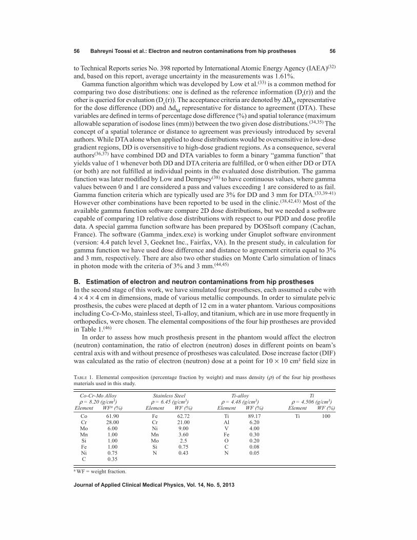
56 Bahreyni toossi et al.: Electron and neutron contaminations from hip prostheses 56
Journal of Applied Clinical Medical Physics, Vol. 14, no. 5, 2013
to Technical Reports series No. 398 reported by International Atomic Energy Agency (IAEA)(32) and, based on this report, average uncertainty in the measurements was 1.61%.
Gamma function algorithm which was developed by Low et al.(33) is a common method for comparing two dose distributions: one is defined as the reference information (Dr(r)) and the other is queried for evaluation (Dc(r)). The acceptance criteria are denoted by ΔDM representative for the dose difference (DD) and ΔdM representative for distance to agreement (DTA). These variables are defined in terms of percentage dose difference (%) and spatial tolerance (maximum allowable separation of isodose lines (mm)) between the two given dose distributions.(34,35) The concept of a spatial tolerance or distance to agreement was previously introduced by several authors. While DTA alone when applied to dose distributions would be oversensitive in low-dose gradient regions, DD is oversensitive to high-dose gradient regions. As a consequence, several authors(36,37) have combined DD and DTA variables to form a binary “gamma function” that yields value of 1 whenever both DD and DTA criteria are fulfilled, or 0 when either DD or DTA (or both) are not fulfilled at individual points in the evaluated dose distribution. The gamma function was later modified by Low and Dempsey(38) to have continuous values, where gamma values between 0 and 1 are considered a pass and values exceeding 1 are considered to as fail. Gamma function criteria which are typically used are 3% for DD and 3 mm for DTA.(33,39-41) However other combinations have been reported to be used in the clinic.(38,42,43) Most of the available gamma function software compare 2D dose distributions, but we needed a software capable of comparing 1D relative dose distributions with respect to our PDD and dose profile data. A special gamma function software has been prepared by DOSIsoft company (Cachan, France). The software (Gamma_index.exe) is working under Gnuplot software environment (version: 4.4 patch level 3, Geeknet Inc., Fairfax, VA). In the present study, in calculation for gamma function we have used dose difference and distance to agreement criteria equal to 3% and 3 mm, respectively. There are also two other studies on Monte Carlo simulation of linacs in photon mode with the criteria of 3% and 3 mm.(44,45)
B. Estimation of electron and neutron contaminations from hip prostheses In the second stage of this work, we have simulated four prostheses, each assumed a cube with 4 × 4 × 4 cm in dimensions, made of various metallic compounds. In order to simulate pelvic prosthesis, the cubes were placed at depth of 12 cm in a water phantom. Various compositions including Co-Cr-Mo, stainless steel, Ti-alloy, and titanium, which are in use more frequently in orthopedics, were chosen. The elemental compositions of the four hip prostheses are provided in Table 1.(46)
In order to assess how much prosthesis present in the phantom would affect the electron (neutron) contamination, the ratio of electron (neutron) doses in different points on beam’s central axis with and without presence of prostheses was calculated. Dose increase factor (DIF) was calculated as the ratio of electron (neutron) dose at a point for 10 × 10 cm² field size in
Table 1. Elemental composition (percentage fraction by weight) and mass density (ρ) of the four hip prostheses materials used in this study.
Co-Cr-Mo Alloy Stainless Steel Ti-alloy Ti ρ = 8.20 (g/cm3) ρ = 6.45 (g/cm3) ρ = 4.48 (g/cm3) ρ = 4.506 (g/cm3) Element WFa (%) Element WF (%) Element WF (%) Element WF (%) Co 61.90 Fe 62.72 Ti 89.17 Ti 100 Cr 28.00 Cr 21.00 Al 6.20 Mo 6.00 Ni 9.00 V 4.00 Mn 1.00 Mn 3.60 Fe 0.30 Si 1.00 Mo 2.5 O 0.20 Fe 1.00 Si 0.75 C 0.08 Ni 0.75 N 0.43 N 0.05 C 0.35
a WF = weight fraction.

57 Bahreyni toossi et al.: Electron and neutron contaminations from hip prostheses 57
Journal of Applied Clinical Medical Physics, Vol. 14, no. 5, 2013
presence of prosthesis to that at the same point in absence of prosthesis. DIF values for total dose were also presented as tabulate data. Total dose in case of electron contamination was cal-culated as electron dose plus photon dose. Total dose for neutron contamination was calculated as neutron dose plus photon dose. In order to calculate electron contamination, we have used two types of input files: one for a free water phantom and one with presence of prosthesis on the beam’s central axis in the water phantom. The electron dose values on the central axis of the beam were calculated for these types of input files. Each prosthesis material was studied by a separate input file. In these calculations, SSD was set to 100 cm and the field size was 10 × 10 cm². SSW and SSR cards have been used in the same way as were used for PDD and dose profile calculations. Photons and electrons were scored on a horizontal plane located at 19.7 cm from the source in the first run file. In the second run file, 35 × 107 particles were read from the plane and electron dose was scored at 1–29 cm depths in the water phantom. The scoring cells were cylinders with 1 cm radius and 2 mm height. The energy deposition was calculated in the scoring cells using *F8 tally. Since the photon doses were required for calculation of DIF for total dose (electron dose + photon dose), the photon doses were calculated using *F8 and F6 tallies in the same tally cells used for calculation of electron dose. In this case, *F8 tally was utilized for calculation of photon dose in depths ranging from 0.1–2.9 cm, and F6 tally in depths of 3.1–21 cm. The input files used for calculation of photon dose were run for about 1.41 × 10⁸ particles and the Monte Carlo errors in the tally cells were less than 3.81%. Except for cutoff and cell importance, no other variance reduction method was used. Energy cutoff for both electrons and photons were set at 10 keV and cell importance was increased in the range of 100–600 in the water phantom with increasing depth.
Neutron contamination was also calculated under similar conditions as for electrons. In other words, SSD, field size, scoring cells, and the types of input files and the implemented variance reduction methods were the same as described above for electron contamination simulations. However, there were some differences in the neutron dose estimations. Based on the resulted errors in neutron dose calculations by running a single input file for 2 × 10⁹ particle histories, it was estimated that it should run an input file for a number of times and then the errors be combined from each run to have an acceptable error level. However, it was necessary to change the random seed number of the input file in each run to have a distinct run. In each input file, source particles were transported directly into a single run and the neutron dose was scored at various depths in the water phantom. For those programs which included prosthesis, each input file has been run 25 times (a total number of 5 × 10¹⁰ source particle histories for each file). The program which did not include prosthesis was run 50 times (a total number of 1011 source particle histories). Energy cutoff for both electrons and photons were defined as 7 MeV in all input files. The neutron flux in the scoring cells was scored using F4 tally and then was converted to neutron equivalent dose rate (rem/h) using DE and DF cards. Neutron flux to equivalent dose rate conversion factors were extracted from Appendix H (Table H-1) of MCNPX (version 2.6.0) manual.(30) DIFs for total dose in the case of neutron contamination are presented as tabulated data. Herein the total dose was calculated as neutron dose plus photon dose. Photon dose needed for calculation of total dose was obtained utilizing F4 tally (flux) for photons. The F4 tally output values were then converted to photon doses (rem/h) using DE and DF cards extracted from Appendix H (Table H-2) of MCNPX (version 2.6.0) manual.(30) While the input files in calculation of photon dose were run for about 1.40 × 10⁸ particles, the maximum Monte Carlo error in the tally cells was 1.36%. The method for calculation of com-bined uncertainties of DIF values for neutron contamination was the same as aforementioned for electron contamination.
In calculation of uncertainties in DIF values, uncertainty of dose at each point for the case presence of prosthesis was extracted from Monte Carlo output. The uncertainty of dose for the case of absence of prosthesis was also derived from the output. The combined uncertainties for division operation were calculated for various depths and prosthesis types and were reported in the tabulated data of DIF. Since the DIFs for total doses were obtained through division of

58 Bahreyni toossi et al.: Electron and neutron contaminations from hip prostheses 58
Journal of Applied Clinical Medical Physics, Vol. 14, no. 5, 2013
total dose following presence of prosthesis to that in absence of prosthesis and the total dose is the summation of electron (neutron) dose by photon dose, the uncertainties related to the summation and division operations were combined toward calculation of uncertainties in DIF for total dose.
III. RESULtS
A. Percent depth dose and dose profiles Percentage depth dose values which were obtained by MC simulations and measurements for 15 MV photon beam are plotted in Fig. 2. The data in the figure are related to 6 × 6, 10 × 10, and 18 × 18 cm² field sizes and SSD of 100 cm. As it was mentioned in the previous section, comparisons of the simulation and measurement data were based on gamma function calcula-tions. The resulted gamma function values used for PDD comparisons for these three field sizes have been plotted in Fig. 3. Gamma calculations were performed using dose difference and distance to agreement criteria of 3% and 3 mm, respectively. As it can be seen from the gamma data in Fig. 3, only few points are having gamma values greater than unity, which is interpreted as fail or disagreement at these points. The points are related only to a few numbers of depths for 6 × 6 and 10 × 10 cm² field sizes. The number of points with gamma index of higher than unity were 11, 3, and 0 points for 6 × 6, 10 × 10, and 18 × 18 cm² field sizes, respectively. It should be noted that we have selected the calculation points very close to each other in the build-up region. This resulted in a greater number of points with gamma index of higher than unity for the 6 × 6 cm2 field.
Dose profiles related to the three field sizes of 6 × 6, 10 × 10, and 18 × 18 cm² for three depths of 5, 10, and 20 mm, obtained from Monte Carlo simulations and measurements, are respectively plotted in Figs. 4(a)–4(c), respectively. The corresponding gamma values for dose profile data for the three fields are plotted in Fig. 5. Figures 5(a), (b), and (c) illustrate gamma function results for dose profiles at 5, 10, and 20 cm depths, respectively. All the gamma cal-culations were performed by defining 3% dose difference and 3 mm distance to agreement criteria. From nine cases of gamma plots related to dose profiles (for three field sizes and three depths), we have only selected three sample cases to be plotted in Fig. 5. Among nine cases
Fig. 2. Percent depth dose values for 15 MV photon beam calculated by MC code versus measurement data (SSD = 100). The curves (a), (b) and (c) are corresponding to 6 × 6, 10 × 10, and 18 × 18 cm² field sizes, respectively. For more clarification, the data for 6 × 6 and 10 × 10 cm² field sizes are scaled 0.8 and 0.9, respectively.
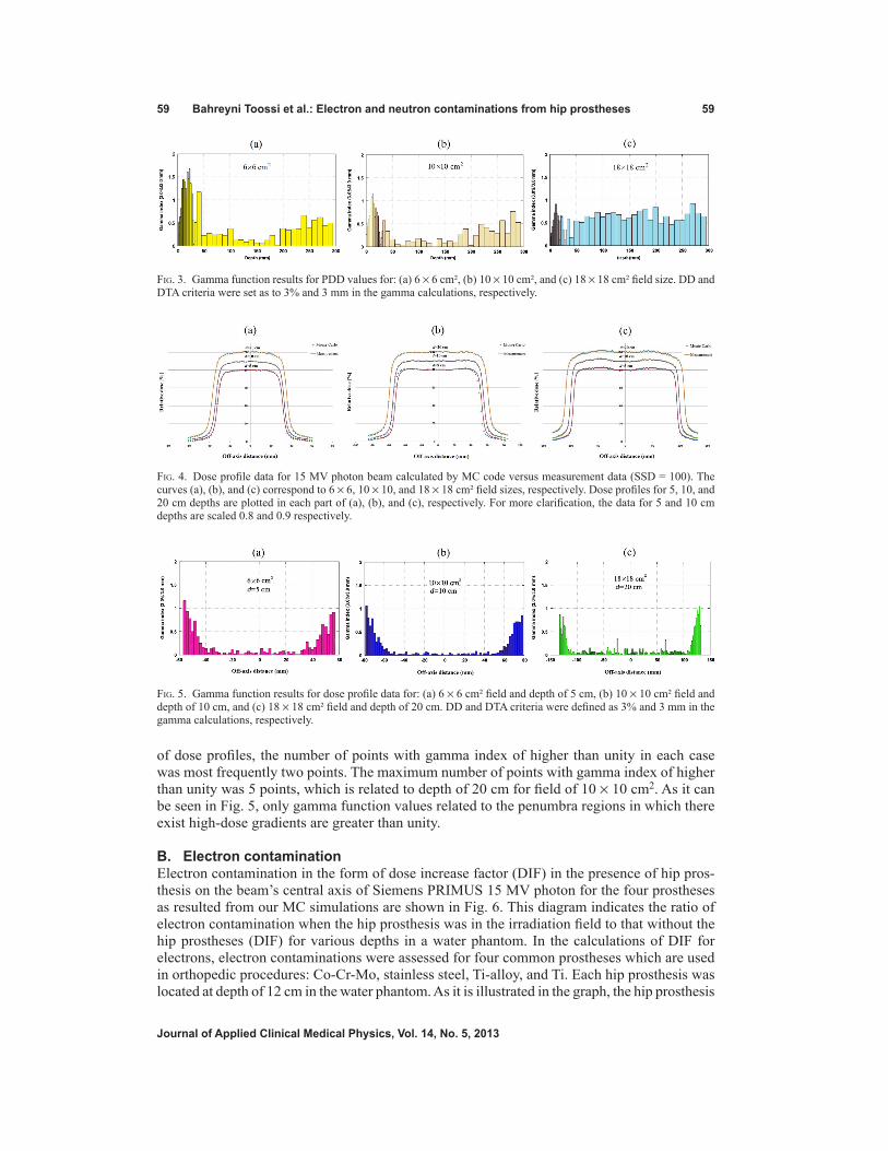
59 Bahreyni toossi et al.: Electron and neutron contaminations from hip prostheses 59
Journal of Applied Clinical Medical Physics, Vol. 14, no. 5, 2013
of dose profiles, the number of points with gamma index of higher than unity in each case was most frequently two points. The maximum number of points with gamma index of higher than unity was 5 points, which is related to depth of 20 cm for field of 10 × 10 cm2. As it can be seen in Fig. 5, only gamma function values related to the penumbra regions in which there exist high-dose gradients are greater than unity.
B. Electron contaminationElectron contamination in the form of dose increase factor (DIF) in the presence of hip pros-thesis on the beam’s central axis of Siemens PRIMUS 15 MV photon for the four prostheses as resulted from our MC simulations are shown in Fig. 6. This diagram indicates the ratio of electron contamination when the hip prosthesis was in the irradiation field to that without the hip prostheses (DIF) for various depths in a water phantom. In the calculations of DIF for electrons, electron contaminations were assessed for four common prostheses which are used in orthopedic procedures: Co-Cr-Mo, stainless steel, Ti-alloy, and Ti. Each hip prosthesis was located at depth of 12 cm in the water phantom. As it is illustrated in the graph, the hip prosthesis
Fig. 3. Gamma function results for PDD values for: (a) 6 × 6 cm², (b) 10 × 10 cm², and (c) 18 × 18 cm² field size. DD and DTA criteria were set as to 3% and 3 mm in the gamma calculations, respectively.
Fig. 4. Dose profile data for 15 MV photon beam calculated by MC code versus measurement data (SSD = 100). The curves (a), (b), and (c) correspond to 6 × 6, 10 × 10, and 18 × 18 cm² field sizes, respectively. Dose profiles for 5, 10, and 20 cm depths are plotted in each part of (a), (b), and (c), respectively. For more clarification, the data for 5 and 10 cm depths are scaled 0.8 and 0.9 respectively.
Fig. 5. Gamma function results for dose profile data for: (a) 6 × 6 cm² field and depth of 5 cm, (b) 10 × 10 cm² field and depth of 10 cm, and (c) 18 × 18 cm² field and depth of 20 cm. DD and DTA criteria were defined as 3% and 3 mm in the gamma calculations, respectively.

60 Bahreyni toossi et al.: Electron and neutron contaminations from hip prostheses 60
Journal of Applied Clinical Medical Physics, Vol. 14, no. 5, 2013
(with dimensions of 4 × 4 × 4 cm) is located in the depth of 12 cm in the phantom. A numerical data of the DIF values for electron contamination are also listed in Table 2. DIF values related to total dose (electron dose + photon dose) for the four prostheses are presented in Table 3.
Fig. 6. Dose increase factor (DIF) vs. depth for electron contamination in presence of hip prostheses in the 15 MV photon beam pathway for the four hip prostheses: Co-Cr-Mo, stainless steel, Ti, and Ti-alloy.

61 Bahreyni toossi et al.: Electron and neutron contaminations from hip prostheses 61
Journal of Applied Clinical Medical Physics, Vol. 14, no. 5, 2013
Table 2. Dose increase factor (DIF) assigned to electron contamination in a 15 MV photon beam produced by four prostheses: Co-Cr-Mo, Stainless steel, Ti-alloy, and Ti in a water phantom.
Dose Increase Factor (DIF) ± Uncertainty Depth in Phantom Stainless (cm) Co-Cr-Mo Steel Ti-alloy Ti
5 1.01±0.02 1.01±0.02 1.01±0.02 1.01±0.02 6 1.01±0.02 1.01±0.02 1.01±0.02 1.04±0.02 7 1.00±0.02 0.99±0.02 0.98±0.02 0.99±0.02 8 1.00±0.02 0.99±0.02 0.99±0.02 1.00±0.02
Water 8.9 1.01±0.03 1.00±0.03 0.99±0.03 1.00±0.03 9.1 0.99±0.03 0.99±0.03 0.98±0.03 0.98±0.03 9.3 0.98±0.03 0.98±0.03 0.96±0.02 0.97±0.02 9.5 1.02±0.03 1.02±0.03 1.00±0.03 1.00±0.03 9.7 1.06±0.03 1.06±0.03 1.05±0.03 1.04±0.03 9.9 1.18±0.03 1.16±0.03 1.16±0.03 1.14±0.03 10.1 1.07±0.02 1.05±0.02 0.98±0.03 1.00±0.02 10.3 1.09±0.02 1.10±0.03 1.03±0.03 1.02±0.02 10.5 1.06±0.02 1.08±0.03 1.02±0.03 1.01±0.02 10.7 1.05±0.02 1.08±0.03 1.04±0.03 1.03±0.02 10.9 1.02±0.02 1.06±0.02 0.99±0.02 1.03±0.03 11.1 0.98±0.02 1.03±0.02 0.97±0.02 0.98±0.02 11.3 0.98±0.02 1.02±0.02 1.03±0.03 1.01±0.02 11.5 0.93±0.02 0.98±0.02 1.01±0.03 1.02±0.03 11.7 0.88±0.02 0.95±0.02 0.96±0.02 0.97±0.02
Prosthesis 11.9 0.86±0.02 0.92±0.02 0.93±0.02 0.98±0.02 12.1 0.82±0.02 0.87±0.02 0.90±0.02 0.90±0.02 12.3 0.79±0.02 0.86±0.02 0.89±0.02 0.88±0.02 12.5 0.74±0.02 0.82±0.02 0.85±0.02 0.85±0.02 12.7 0.70±0.02 0.78±0.02 0.83±0.02 0.83±0.02 12.9 0.71±0.02 0.78±0.02 0.83±0.02 0.84±0.02 13.1 0.67±0.02 0.75±0.02 0.84±0.02 0.84±0.02 13.3 0.64±0.02 0.73±0.02 0.81±0.02 0.82±0.02 13.5 0.62±0.02 0.71±0.02 0.81±0.02 0.82±0.02 13.7 0.60±0.02 0.71±0.02 0.79±0.02 0.80±0.02 13.9 0.55±0.01 0.64±0.02 0.72±0.02 0.72±0.02 14.1 0.57±0.02 0.68±0.02 0.80±0.03 0.79±0.02 14.9 0.52±0.02 0.64±0.02 0.74±0.02 0.72±0.02 15.9 0.47±0.02 0.56±0.02 0.70±0.02 0.69±0.02
Water 17 0.48±0.02 0.58±0.02 0.73±0.02 0.70±0.02 18 0.48±0.02 0.57±0.02 0.70±0.02 0.71±0.02 19 0.47±0.02 0.56±0.02 0.72±0.02 0.72±0.02 20 0.48±0.02 0.56±0.02 0.73±0.03 0.72±0.03 21 0.46±0.02 0.56±0.02 0.69±0.03 0.69±0.02

62 Bahreyni toossi et al.: Electron and neutron contaminations from hip prostheses 62
Journal of Applied Clinical Medical Physics, Vol. 14, no. 5, 2013
C. neutron contaminationNeutron contaminations in the form of DIF for neutrons in the presence of hip prosthesis on the central axis of beam are shown in Fig. 7. The data were obtained from MC simulations of the four hip prostheses when they are located at depth of 12 cm in a water phantom in a 10 × 10 cm2 field of a 15 MV Siemens PRIMUS linac. This figure demonstrates the ratio of neutron dose with presence to that in the absence of hip prosthesis in the irradiation field (DIF) for the four prostheses materials. Dimensions of hip prosthesis in the simulation were 4 × 4 × 4 cm. Besides the graphical presentation of neutron contaminations in Fig. 7, numerical data of DIF values related to neutron productions from Co-Cr-Mo, stainless steel, Ti-alloy, and Ti prostheses are listed in Table 4. DIF values corresponding to total dose (neutron dose + photon dose) for the four prostheses are listed in Table 5.
Table 3. Dose increase factor (DIF) assigned to total dose (electron dose + photon dose) in a 15 MV photon beam produced by four prostheses: Co-Cr-Mo, Stainless steel, Ti-alloy, and Ti in a water phantom.
Dose Increase Factor (DIF) ± Uncertainty Depth in Phantom Stainless (cm) Co-Cr-Mo Steel Ti-alloy Ti
5 1.01±0.02 1.00±0.02 1.00±0.02 1.00±0.02 6 1.01±0.02 1.01±0.02 1.01±0.02 1.01±0.02 7 1.00±0.02 0.99±0.02 0.98±0.02 0.99±0.02 8 1.00±0.02 0.99±0.02 0.99±0.02 0.99±0.02
Water 8.9 1.01±0.03 1.00±0.03 0.99±0.03 1.00±0.03 9.1 0.99±0.03 0.99±0.02 0.98±0.02 0.98±0.02 9.3 0.98±0.02 0.98±0.03 0.96±0.02 0.97±0.02 9.5 1.02±0.03 1.02±0.03 1.00±0.03 1.00±0.03 9.7 1.06±0.03 1.06±0.03 1.05±0.03 1.04±0.03 9.9 1.18±0.03 1.16±0.03 1.16±0.03 1.14±0.03 10.1 1.07±0.02 1.05±0.02 0.98±0.02 0.99±0.02 10.3 1.09±0.02 1.10±0.03 1.02±0.02 1.02±0.02 10.5 1.05±0.02 1.08±0.02 1.02±0.02 1.01±0.02 10.7 1.05±0.02 1.08±0.02 1.04±0.02 1.03±0.02 10.9 1.02±0.02 1.06±0.02 0.99±0.02 1.03±0.02 11.1 0.98±0.02 1.03±0.02 0.97±0.02 0.98±0.02 11.3 0.98±0.02 1.02±0.02 1.02±0.02 1.01±0.02 11.5 0.93±0.02 0.98±0.02 1.01±0.03 1.02±0.03 11.7 0.88±0.02 0.95±0.02 0.96±0.02 0.97±0.02
Prosthesis 11.9 0.85±0.02 0.92±0.02 0.93±0.02 0.97±0.02 12.1 0.81±0.02 0.87±0.02 0.90±0.02 0.90±0.02 12.3 0.79±0.02 0.86±0.02 0.89±0.02 0.88±0.02 12.5 0.74±0.02 0.82±0.02 0.85±0.02 0.85±0.02 12.7 0.70±0.02 0.77±0.02 0.83±0.02 0.83±0.02 12.9 0.71±0.02 0.78±0.02 0.83±0.02 0.84±0.02 13.1 0.67±0.02 0.75±0.02 0.84±0.02 0.83±0.02 13.3 0.64±0.02 0.73±0.02 0.81±0.02 0.82±0.02 13.5 0.62±0.02 0.71±0.02 0.81±0.02 0.82±0.02 13.7 0.60±0.02 0.71±0.02 0.79±0.02 0.80±0.02 13.9 0.55±0.01 0.64±0.02 0.72±0.02 0.72±0.02 14.1 0.57±0.02 0.68±0.02 0.80±0.03 0.78±0.02 14.9 0.52±0.02 0.63±0.02 0.74±0.02 0.72±0.02 15.9 0.47±0.02 0.56±0.02 0.69±0.02 0.69±0.02
Water 17 0.48±0.02 0.58±0.02 0.73±0.02 0.70±0.02 18 0.48±0.02 0.57±0.02 0.70±0.02 0.71±0.02 19 0.47±0.02 0.56±0.02 0.72±0.02 0.72±0.02 20 0.48±0.02 0.56±0.02 0.72±0.03 0.71±0.02 21 0.46±0.02 0.56±0.02 0.69±0.02 0.69±0.02

63 Bahreyni toossi et al.: Electron and neutron contaminations from hip prostheses 63
Journal of Applied Clinical Medical Physics, Vol. 14, no. 5, 2013
Fig. 7. Dose increase factor (DIF) vs. depth for neutron contamination in presence of hip prostheses in the 15 MV photon beam pathway for the four hip prostheses: Co-Cr-Mo, Stainless steel, Ti-alloy, and Ti.
Table 4. Dose increase factor (DIF) assigned to neutron contamination in a 15 MV photon beam produced by four prostheses: Co-Cr-Mo, Stainless steel, Ti-alloy, and Ti in a water phantom.
Dose Increase Factor (DIF) ± Uncertainty Depth in Phantom Stainless (cm) Co-Cr-Mo Steel Ti-alloy Ti
1 1.05±0.11 1.02±0.10 1.04±0.10 1.06±0.10 2 1.04±0.10 1.00±0.09 1.01±0.09 1.04±0.10 3 1.03±0.10 0.97±0.10 0.96±0.09 1.01±0.10
Water 4 0.99±0.11 0.92±0.10 0.90±0.09 0.96±0.10 5 1.05±0.12 0.93±0.11 0.84±0.10 0.98±0.11 6 1.71±0.19 1.37±0.17 0.99±0.12 1.09±0.14 7 5.85±0.61 4.58±0.55 1.90±0.23 2.17±0.27 8 36.85±4.12 26.27±3.16 8.05±0.96 9.09±1.08 9 184.55±21.80 137.33±18.75 40.66±4.93 43.17±5.20 11 2197.63±298.29 1593.77±228.52 468.48±63.86 524.81±71.4 Prosthesis 12 1229.37±171.61 925.15±132.63 277.89±38.96 311.25±43.58 13 1729.75±247.97 1347.23±105.44 422.54±40.84 471.48±67.80 15 138.49±10.99 110.58±16.92 36.86±3.06 40.77±3.37 16 31.05±4.79 23.49±3.62 8.49±1.36 9.49±1.51 17 8.84±1.39 6.68±1.20 2.25±0.38 2.63±0.44
Water 18 2.86±0.53 2.17±0.42 0.93±0.19 1.15±0.23 19 0.94±0.19 0.88±0.17 0.58±0.13 0.79±0.18 20 0.39±0.08 0.71±0.16 0.60±0.12 0.49±0.11 21 0.40±0.10 0.71±0.18 0.46±0.12 0.49±0.13 22 0.83±0.26 0.45±0.13 0.49±0.15 0.46±0.15

64 Bahreyni toossi et al.: Electron and neutron contaminations from hip prostheses 64
Journal of Applied Clinical Medical Physics, Vol. 14, no. 5, 2013
IV. dISCUSSIon
It is evident from Figs. 2 and 3 that there is a good agreement between our PDD values obtained by Monte Carlo simulations of linac head and the measured values. However, there are only a few points in gamma function data which have gamma values greater than unity which are related to high-dose gradient parts in the build-up region. For dose profiles, as plotted in Fig. 5, it can be noted that there are few points with gamma indexes greater than unity. These points are those located in the penumbra region or out of the radiation field. Generally speaking, there is a good agreement between our simulations and measurements of PDDs and dose profile. Therefore, our Monte Carlo model of the linac head is validated.
Evaluations of electron contaminations from the four hip prostheses (Fig. 6 and Table 2) are clearly indicating that electron contamination from Co-Cr-Mo prosthesis is higher than that of other prostheses. Maximum DIFs for electron contamination in the presence of prostheses are equal to 1.18, 1.16, 1.16 and 1.14 for Co-Cr-Mo, stainless steel, Ti, and Ti-alloy, respectively. The dominant photon interaction in energies higher than 10 MeV is pair production and when a photon undergoes a pair production interaction, electron is produced. The probability of pair production is proportional to the square of atomic number (Z²). Atomic number of Co, Fe, and Ti (the most frequent elements in the Co-Cr-Mo, stainless steel, and Ti alloys) are 27, 26, and 22, respectively. Therefore, it can be expected that Co-Cr-Mo alloy would have the highest electron contamination production, followed by stainless steel, etc. When comparing DIF for electron contamination production by Ti-alloy and Ti, the difference can be related to presence of V in Ti-alloy with atomic number of 23, which does not exist in Ti prosthesis. Another effect that can be noticed from the data presented in Table 2 is the fact that electron contamination is increased before the hip prosthesis. This effect can be related to back-scattered electrons from the prosthesis. This increase is seen up to a range of 3–5 mm away from hip prostheses. Electron contamination is reduced beyond prosthesis as a result of absorption of electrons in
Table 5. Dose increase factor (DIF) assigned to total dose (neutron dose + photon dose) in a 15 MV photon beam produced by four prostheses: Co-Cr-Mo, Stainless steel, Ti-alloy, and Ti in a water phantom.
Dose Increase Factor (DIF) ± Uncertainty Depth in Phantom Stainless (cm) Co-Cr-Mo Steel Ti-alloy Ti
1 1.00±0.08 1.00±0.08 1.00±0.08 1.00±0.08 2 0.99±0.08 1.00±0.08 0.99±0.08 1.01±0.08 3 1.01±0.10 0.99±0.09 1.00±0.09 0.99±0.09
Water 4 1.00±0.02 1.00±0.02 0.99±0.02 1.00±0.02 5 1.00±0.02 1.00±0.02 1.00±0.02 1.00±0.02 6 1.00±0.02 1.00±0.02 1.00±0.02 1.00±0.02 7 1.00±0.02 1.00±0.02 1.00±0.02 1.00±0.02 8 1.00±0.02 1.00±0.02 1.00±0.02 1.00±0.02 9 1.00±0.02 1.00±0.02 1.01±0.02 1.00±0.02 11 0.83±0.02 0.86±0.02 0.96±0.02 0.85±0.02 Prosthesis 12 0.68±0.01 0.75±0.02 0.88±0.02 0.79±0.02 13 0.54±0.01 0.63±0.01 0.81±0.02 0.70±0.02 15 0.44±0.01 0.55±0.01 0.69±0.02 0.68±0.02 16 0.43±0.01 0.53±0.01 0.69±0.02 0.67±0.02 17 0.43±0.01 0.52±0.01 0.68±0.02 0.67±0.02
Water 18 0.43±0.01 0.52±0.01 0.68±0.02 0.67±0.02 19 0.43±0.01 0.52±0.01 0.68±0.02 0.66±0.02 20 0.43±0.01 0.52±0.01 0.68±0.02 0.66±0.02 21 0.43±0.01 0.52±0.01 0.67±0.02 0.66±0.02 22 0.43±0.01 0.52±0.01 0.67±0.02 0.66±0.02

65 Bahreyni toossi et al.: Electron and neutron contaminations from hip prostheses 65
Journal of Applied Clinical Medical Physics, Vol. 14, no. 5, 2013
the prosthesis. The electron contamination is increased in some extent within the hip prosthe-ses, but it has no significant effect since there is not any living tissue within the prostheses. The results of DIF for total dose (electron dose plus photon dose), which were presented in Table 3, indicate that the DIFs are showing the same trends as it was in the case of DIFs for electron contamination.
The effect of hip prostheses on neutron contamination on beam’s central axis, as shown in Fig. 7 and Table 4, demonstrate that neutron contamination at the range of 5 cm before and 4 cm beyond the prostheses has been increased in the presence of prosthesis in the phantom. It is clearly shown in Fig. 7 that neutron contamination in presence of prosthesis is increased dramatically within the prosthesis. DIF values for neutron contaminations before prostheses amount to 184.55, 137.33, 40.66, and 43.17 for Co-Cr-Mo, stainless steel, Ti-alloy, and Ti, respectively. This increase is higher for Co-Cr-Mo material, and then for stainless steel, Ti, and Ti-alloy, respectively. It can be noticed from the data in Table 4 that unlike electron contamina-tion, which is decreased beyond prosthesis and is increased only up to few millimeters before the prostheses, neutron contamination is increased both before and beyond the prosthesis. At it can be seen from the data of Table 5, DIF for total dose (neutron dose plus photon dose) is almost equal to 1.00 in the points above each four prostheses. The DIF shows decrease in both within prostheses and after them. It seems that the total dose is affected mainly by photon dose components and therefore it can be mentioned that, from total dose point of view, presence of prosthesis has not any effect on tissues before prosthesis, but it will attenuate the photons and thus the photon dose (and also total dose) after the prostheses is decreased. The decrease in photons dose inside the prostheses may not have any clinical aspect. There is not any previous study on total dose in presence on prostheses, but a previous study by Mesbahi and Nejad(17) has shown similar trends in attenuation of photon dose with depth in presence of prostheses. There are some differences between the two studies, such as the photon energy (15 MV vs. 9 MV), linac model (Siemens PRIMUS vs. NEPTUN 10PC), etc.
V. ConCLUSIonS
In the present study, we have simulated 15 MV photon beam of a Siemens PRIMUS linac by MCNPX MC code, and then electron and neutron dose increase effect due to electron and neu-tron contamination production from four hip prostheses was quantified. Our results have shown that presence of prosthesis in a phantom can increase both electron and neutron contaminations. Generally, the dose increase factor for neutron contamination is more than that for electron contamination. The neutron contamination, which originates from the prosthesis, can penetrate up to a range of 5 cm before the prosthesis and up to a range of 4 cm beyond it. Neutron con-tamination in the absence of hip prosthesis for Siemens PRIMUS linac is low, but it may be increased in the presence of prosthesis up to a factor of 184.55. The increase factor depends on the composition of prosthesis. When we consider the higher RBE of neutrons relative to photons, this effect can be more important with respect to biological damage to the patient.
It is evident from Tables 2 and 4 that Ti-alloy and Ti prosthesis produce less electron and neutron contaminations than the other prostheses. Since a patient with hip junction replacement may undergo pelvic irradiation later in his lifetime, it is recommended to implant a Ti-based alloy (Ti-alloy or Ti) in his/her hip in his/her orthopedic procedure. Furthermore it is recommended to located prosthesis in the high-energy photon beam pathway in the time of radiotherapy treat-ment planning. Based on the results acquired in this study, it is expected that, if a patient has any other type of prosthesis or metallic device implanted in his/her body (e.g., spinal fixation rods, dental restoration, fixed prosthodontics), if these devices are exposed to a high-energy photon beam then there is a high possibility of electron and neutron contamination production. This field calls for further studies on the production of electron or neutron contaminations in high-energy photon beams.

66 Bahreyni toossi et al.: Electron and neutron contaminations from hip prostheses 66
Journal of Applied Clinical Medical Physics, Vol. 14, no. 5, 2013
Presence of hip prosthesis can highly affect the total doses (electron dose plus photon dose; neutron dose plus photon dose). The total doses are reduced at depths after prosthesis in both cases of electron and neutron contaminations. This effect is due to attenuation of various par-ticles inside the prosthesis, and is clinically important. Additionally the total dose in the case of electron contamination shows in depths increase before the prosthesis. This will increase the soft tissue dose which exists before hip bone. Taking into account these effects by clinical treatment planning systems may have influences on the treatment outcomes and, thus, it is recommended that the effects be considered in the process of treatment planning of a patient with hip prosthesis.
ACknowLEdgMEntS
We are thankful to Dr. Faezeh Rahmani for her help in solving the neutron transport problems. The authors would also like to thank Reza Radiation Oncology Center (Mashhad, Iran) for providing the experimental data. The results of this study were extracted from the data of a research project under the grant number 900445, which was financially supported by Mashhad University of Medical Sciences (MUMS).
REFEREnCES
1. Reft C, Alecu R, Das IJ, et al. Dosimetric considerations for patients with HIP prostheses undergoing pelvic irra-diation. Report of the AAPM Radiation Therapy Committee Task Group 63. Med Phys. 2003;30(6):1162–82.
2. Mesbahi A. A Monte Carlo study on neutron and electron contamination of an unflattened 18-MV photon beam. Appl Radiat Isot. 2009;67(1):55–60.
3. Petti PL, Goodman MS, Sisterson JM, Biggs PJ, Gabriel TA, Mohan R. Sources of electron contamination for the Clinac-35 25-MV photon beam. Med Phys. 1983;10(6):856–61.
4. Lopez Medina A, Teijeiro A, Garcia J, et al. Characterization of electron contamination in megavoltage photon beams. Med Phys. 2005;32(5):1281–92.
5. Butson MJ, Cheung T, Yu PKN, Carolan M, Metcalfe PE. Simulation and measurement of air generated electron contamination in radiotherapy. Radiat Meas. 2000;32(2):105–11.
6. Butson MJ, Cheung T, Yu PKN. Lepton contamination and photon scatter produced by open field 18 MV X-ray beams in the build-up region. Radiat Meas. 2002;35(2):103–07.
7. Petti PL, Goodman MS, Gabriel TA, Mohan R. Investigation of buildup dose from electron contamination of clinical photon beams. Med Phys. 1983;10(1):18–24.
8. Martinez-Ovalle SA, Barquero R, Gomez-Ros JM, Lallena AM. Neutron dose equivalent and neutron spectra in tissue for clinical linacs operating at 15, 18 and 20 MV. Radiat Prot Dosimetry. 2011;147(4):498–511.
9. Becker J, Brunckhorst E, Schmidt R. Investigation of the neutron contamination in IMRT deliveries with a paired magnesium and boron coated magnesium ionization chamber system. Radiother Oncol. 2008;86(2):182–86.
10. Gomez F, Iglesias A, Doblado FS. A new active method for the measurement of slow-neutron fluence in modern radiotherapy treatment rooms. Phys Med Biol. 2010;55(4):1025–39.
11. Zanini A, Durisi E, Fasolo F, et al. Monte Carlo simulation of the photoneutron field in linac radiotherapy treat-ments with different collimation systems. Phys Med Biol. 2004;49(4):571–82.
12. Nath R, Boyer AL, LaRiviere PD, McCall RC, and Price KW. Neutron measurements around high energy X-ray radiotherapy machines. A Report of Task Group 27, Radiation Therapy Committee, American Association of Physicists in Medicine. AAPM Report No. 19. New York: Medical Physics Publishing; 1986.
13. Ma A, Awotwi-Pratt J, Alghamdi A, Alfuraih A, Spyrou N. Monte Carlo study of photoneutron production in the Varian Clinac 2100C linac. J Radioanal Nucl Chem. 2008;276(1):119–23.
14. Ongaro C, Zanini A, Nastasi U, et al. Analysis of photoneutron spectra produced in medical accelerators. Phys Med Biol. 2000;45(12):L55–L61.
15. Schneider U, Fiechtner A, Besserer J, Lomax A. Neutron dose from prostheses material during radiotherapy with protons and photons. Phys Med Biol. 2004;49(9):119–24.
16. Laub WU and Nusslin F. Monte Carlo dose calculations in the treatment of a pelvis with implant and comparison with pencil-beam calculations. Med Dosim. 2003;28(4):229–33.
17. Mesbahi A and Nejad FS. Dose attenuation effect of hip prostheses in a 9-MV photon beam: commercial treat-ment planning system versus Monte Carlo calculations. Radiat Med. 2007;25(10):529–35.
18. Buffard E, Gschwind R, Makovicka L, David C. Monte Carlo calculations of the impact of a hip prosthesis on the dose distribution. Nucl Instrum Meth B. 2006;251(1):9–18.
19. Hazuka MB, Ibbott GS, Kinzie JJ. Hip prostheses during pelvic irradiation: effects and corrections. Int J Radiat Oncol Biol Phys. 1988;14(6):1311–17.

67 Bahreyni toossi et al.: Electron and neutron contaminations from hip prostheses 67
Journal of Applied Clinical Medical Physics, Vol. 14, no. 5, 2013
20. Erlanson M, Franzen L, Henriksson R, Littbrand B, Lofroth PO. Planning of radiotherapy for patients with hip prosthesis. Int J Radiat Oncol Biol Phys. 1991;20(5):1093–98.
21. Carolan M, Dao P, Fox C, Metcalfe P. Effect of hip prostheses on radiotherapy dose. Australas Radiol. 2000;44(3):290–95.
22. Lin SY, Chu TC, Lin JP, Liu MT. The effect of a metal hip prosthesis on the radiation dose in therapeutic photon beam irradiations. Appl Radiat Isot. 2002;57(1):17–23.
23. Wieslander E and Knoos T. Dose perturbation in the presence of metallic implants: treatment planning system versus Monte Carlo simulations. Phys Med Biol. 2003;48(20):3295–305.
24. Keall PJ, Siebers JV, Jeraj R, Mohan R. Radiotherapy dose calculations in the presence of hip prostheses. Med Dosim. 2003;28(2):107–12.
25. Chin DW, Treister N, Friedland B, et al. Effect of dental restorations and prostheses on radiotherapy dose distri-bution: a Monte Carlo study. J Appl Clin Med Phys. 2009;10(1):2853.
26. Brunckhorst E. Experimental investigations of the neutron contamination in high-energy photon fields at medical linear accelerators [PhD Thesis]. Department of Physics, University of Humburg; 2009.
27. Sibata CH, Mota HC, Higgins PD, Gaisser D, Saxton JP, Shin KH. Influence of hip prostheses on high energy photon dose distributions. Int J Radiat Oncol Biol Phys. 1990;18(2):455–61.
28. Semilitsch M and Willert HG. Properties of implant alloys for artificial hip joints. Med Biol Eng Comput. 1980;18(4):511–20.
29. Tatcher M and Palti S. Evaluation of density correction algorithms for photon-beam dose calculations. Radiology. 1981;141(1):201–05.
30. Pelowitz D. MCNPX user’s manual, Version 2.6.0. Los Alamos, NM: Los Alamos National Laboratory; 2008. 31. Solberg TD, DeMarco JJ, Chetty IJ, et al. A review of radiation dosimetry applications using the MCNP Monte
Carlo code. Radiochimica Acta. 2001;89(4-5):337–55. 32. International Atomic Energy Agency. Absorbed dose determination in external beam radiotherapy: an international
code of practice for dosimetry based on standards of absorbed dose to water. IAEA TRS-398. Vienna: IAEA; 2004. 33. Low DA, Harms WB, Mutic S, Purdy JA. A technique for the quantitative evaluation of dose distributions. Med
Phys. 1998;25(5):656–61. 34. Depuydt T, Van Esch A, Huyskens DP. A quantitative evaluation of IMRT dose distributions: refinement and
clinical assessment of the gamma evaluation. Radiother Oncol. 2002;62(3):309–19. 35. Mohammadi M, Bezak E, Reich P. The use of extended dose range film for dosimetric calibration of a scanning
liquid-filled ionization chamber electronic portal imaging device. J Appl Clin Med Phys. 2006;8(1):69–84. 36. Cheng A, Harms WB Sr., Gerber RL, Wong JW, Purdy JA. Systematic verification of a three-dimensional electron
beam dose calculation algorithm. Med Phys. 1996;23(5):685–93. 37. Harms WB Sr., Low DA, Wong JW, Purdy JA. A software tool for the quantitative evaluation of 3D dose calcula-
tion algorithms. Med Phys. 1998;25(10):1830–36. 38. Low DA and Dempsey JF. Evaluation of the gamma dose distribution comparison method. Med Phys.
2003;30(9):2455–64. 39. Van Esch A, Depuydt T, Huyskens DP. The use of an aSi-based EPID for routine absolute dosimetric pre-treatment
verification of dynamic IMRT fields. Radiother Oncol. 2004;71(2):223–34. 40. Agazaryan N, Solberg TD, DeMarco JJ. Patient specific quality assurance for the delivery of intensity modulated
radiotherapy. J Appl Clin Med Phys. 2003;4(1):40–50. 41. McDermott LN, Wendling M, van Asselen B, et al. Clinical experience with EPID dosimetry for prostate IMRT
pre-treatment dose verification. Med Phys. 2006;33(10):3921–30. 42. De Martin E, Fiorino C, Broggi S, et al. Agreement criteria between expected and measured field fluences in
IMRT of head and neck cancer: the importance and use of the gamma histograms statistical analysis. Radiother Oncol. 2007;85(3):399–406.
43. Childress NL, White RA, Bloch C, Salehpour M, Dong L, Rosen II. Retrospective analysis of 2D patient-specific IMRT verifications. Med Phys. 2005;32(4):838–50.
44. Grevillot L, Frisson T, Maneval D, Zahra N, Badel JN, Sarrut D. Simulation of a 6 MV Elekta Precise Linac photon beam using GATE/GEANT4. Phys Med Biol. 2011;56(4):903–18.
45. Cho W, Kielar KN, Mok E, et al. Multi source modeling of flattening filter free (FFF) beam and the optimization of model parameters. Med Phys. 2011;38(4):1931–42.
46. Bazalova M, Coolens C, Cury F, Childs P, Beaulieu L, Verhaegen F. Monte Carlo dose calculations for phantoms with hip prostheses. J Phys Conf Ser. 2008;102(1):012001.

a Corresponding author: Vincent WC Wu, Department of Health Technology & Informatics, Hong Kong Polytechnic University, Hung Hom, Kowloon, Hong Kong SAR; phone: (852) 3400 8567; fax: (852) 2362 4365; email: [email protected]
Evaluation of the influence of tumor location and size on the difference of dose calculation between Ray Tracing algorithm and Fast Monte Carlo algorithm in stereotactic body radiotherapy of non-small cell lung cancer using CyberKnife
Vincent W.C. Wu,1a Kwok-wah Tam,2 Shun-ming Tong2
Department of Health Technology & Informatics,1 Hong Kong Polytechnic University, Hung Hom, Hong Kong SAR; Teresa Po CyberKnife Center,2 Hong Kong Adventist Hospital, Wan Chai, Hong Kong [email protected]
Received 5 November, 2012; accepted 26 April, 2013
This study evaluated the extent of improvement in dose predication accuracy achieved by the Fast Monte Carlo algorithm (MC) compared to the Ray Tracing algorithm (RAT) in stereotactic body radiotherapy (SBRT) of non-small cell lung cancer (NSCLC), and how their differences were influenced by the tumor site and size. Thirty-three NSCLC patients treated with SBRT by CyberKnife in 2011 were recruited. They were divided into the central target group (n = 17) and peripheral target group (n = 16) according to the RTOG 0236 guidelines. Each group was further divided into the large and small target subgroups. After the computation of treatment plans using RAT, a MC plan was generated using the same patient data and treatment parameters. Apart from the target reference point dose measure-ments, various dose parameters for the planning target volume (PTV) and organs at risk (OARs) were assessed. In addition, the “Fractional Deviation” (FDev) was also calculated for comparison, which was defined as the ratio of the RAT and MC values. For peripheral lung cases, RAT produced significantly higher dose values in all the reference points than MC. The FDev of all reference point doses and dose parameters was greater in the small target than the large target subgroup. For central lung cases, there was no significant reference point and OAR dose differ-ences between RAT and MC. When comparing between the small target and large target subgroups, the FDev values of all the dose parameters and reference point doses did not show significant difference. Despite the shorter computation time, RAT was inferior to MC, in which the target dose was usually overestimated. RAT would not be recommended for SBRT of peripheral lung tumors regardless of the target size. However, it could be considered for large central lung tumors because its performance was comparable to MC.
PACS number: 87
Key words: Ray Tracing algorithm, Fast Monte Carlo algorithm, CyberKnife, lung cancer, stereotactic body radiotherapy, dose calculation
I. InTRoduCTIon
Lung cancer is one of the most prevalent malignancies worldwide and has the highest mortality. Early stage non–small cell carcinoma of lung (NSCLC) is often treated by stererotactic body radiotherapy (SBRT) using CyberKnife, from which satisfactory results have been reported.(1-5)
JouRnAL oF APPLIEd CLInICAL MEdICAL PHYSICS, VoLuME 14, nuMBER 5, 2013
68 68

69 Wu et al.: dose calculation algorithms in CyberKnife 69
Journal of Applied Clinical Medical Physics, Vol. 14, no. 5, 2013
SBRT is the use of stereotactic radiotherapy outside the cranium, in which multiple radiation beams are directed at a relatively small target with high precision. CyberKnife (Accuray Inc., Sunnyvale, CA) is a frameless image-guided radiosurgical system that delivers radiation treat-ment using a robot-mounted 6 MV compact linear accelerator. The highly flexible nonisocentric beam delivery facilitates the implementation of stereotactic body radiotherapy (SBRT), which is a highly conformal treatment with steep dose gradients at the target-normal tissue boundary.(6)
Since SBRT delivers relatively high dose per fraction in small number of fractions, accurate dose prediction in the treatment region during treatment planning is essential to understand-ing the dose levels to the target volumes and normal organs, and it is generated by the dose calculation algorithms in the radiotherapy treatment planning system (TPS). Currently, the overall dosimetric accuracy in radiotherapy recommended by AAPM is 5%, in which the dose calculation should be kept within 3%.(7) The situation becomes more challenging when the treatment site contains complex heterogeneous tissue densities, in which the dose calculation algorithm has to correct for the effects of transient electronic disequilibrium between the tissue interfaces.(8) Lung tumor is a soft tissue tumor surrounded by lung tissue, thoracic bone cage (ribs and spine), and the mediastinal soft tissues. These tissues have very different densities and can be a challenge in accurate dose calculation at the different tissue interfaces, especially for the small radiation fields used in CyberKnife.(9)
The Ray Tracing (RAT) algorithm has been used by the Cyberknife Multiplan TPS for the planning of CyberKnife treatments. RAT belongs to the correction-based algorithm, in which the off-center ratio, tissue-phantom ratio, and collimator output factor that are measured under reference conditions, are corrected for the patient’s geometry. The absorbed dose is calculated by assuming the effective depth as determined by the density variation along the beam path. RAT does not take into account effects arising due to the variation of tissue het-erogeneity and electronic disequilibrium at tissue interface, and therefore is regarded as a less accurate algorithm.
Recently, the Fast Monte Carlo (MC) algorithm, which is a modification of the full Monte Carlo simulation, has been introduced in the CyberKnife Multiplan. MC algorithm predicts the absorbed dose by simulating the electron and photons transport based on a probability distribution derived from the first principles. MC algorithm takes into account the electronic disequilibrium, and is generally accepted as the most accurate algorithm at present. However, the main trade-off is its relatively long processing time. Recently, MC algorithm has been introduced in the CyberKnife TPS with a range of “uncertainty levels” from 0.1% to 4%, in which the higher uncertainty level is associated with less number of photon simulation his-tories, and therefore is less accurate. Our study aimed to evaluate how much improvement in dose predication accuracy could be achieved by MC algorithm when compared to the RAT algorithm in the SBRT treatment of NSCLC, and how their differences were influenced by the tumor site and size.
II. MATERIALS And METHodS
This is a retrospective study on 33 stage I and II NSCLC patients treated with SBRT by CyberKnife in 2011. They were divided into the central target group (n = 17) and peripheral target groups (n = 16) with reference to the descriptions from trial of the Lung Cancer Stereotactic Radiotherapy versus Surgery (STARS) in RTOG-0236.(10) The central lesion was defined as tumor within 2 cm from the mediastinum, pulmonary, and vertebral structures, whereas tumors arising from the rest of the lung were classified as peripheral lesions. In addition, in order to study the effect of tumor size on the dosimetric outcome, each group was further divided into the large and small target subgroups according to the criterion suggested by van der Voort van Zyp et al.,(11) in which the large target subgroup referred to planning target volume (PTV) of over 27 cm3, while the small target subgroup referred to PTV of smaller than 27 cm3.

70 Wu et al.: dose calculation algorithms in CyberKnife 70
Journal of Applied Clinical Medical Physics, Vol. 14, no. 5, 2013
The original treatment plan (RAT Plan) of each patient was computed with the CT taken when the patient was in normal breathing condition. The CT images (1.5 mm thick) were loaded into the CyberKnife Multiplan (Version 4.1) TPS, in which the PTV (by adding 5 mm to the clinical target volume) and organs at risk (OARs) including the spinal cord, oesophagus, and lung were contoured. The treatment plan followed the protocol of the local department in which a tumor dose of 50 Gy in 3 to 5 fractions was prescribed to the PTV at the 80% isodose level. The prescribed dose should at least cover 95% volume of the PTV, and the dose coverage of PTV should fall between -10% and +25% of the prescribed dose. All treatments were delivered using cone collimation. No avoidance zone was applied and the total number of beams (nodes) for each patient was between 112 and 195. After setting the dose constraints to the targets and OARs, a treatment plan was generated through the sequential optimization process. Isodose display was obtained after dose calculation using the RAT algorithm. The computation grid used for calculation was 1.5 mm2. Using the same patient data, same beam number, directions, weights, and monitor units, another treatment plan (MC Plan) was generated using the same TPS with the MC algorithm set at 1% uncertainty level. The reason for using 1% uncertainty level is it was relatively accurate and with a reasonable operation time. The Fast Monte Carlo algorithm improved the speed of computation, and it was reported to be within ± 0.5% relative to the MC calculation in hetereogeneous conditions using phantom by Ma et al.(12)
Reference point doses were used to analyze the dosimetric information. These reference points were defined at the anterior, posterior, lateral, and medial boundaries of the PTV in each corresponding slice (Figs. 1 and 2). These points were situated at or close to the tumor–lung or tumor–soft tissue interface and sites of steep dose gradient, which were most challenging to the dose calculation algorithms, and at the same time affected the dosimetric prediction of the target. The total number of reference points for each patient was between 48 and 60. Apart from the reference point dose measurements, other dosimetric parameters of the target and OARs (ipsilateral lung, oesophagus, and spinal cord) were also compared. The PTV coverage was assessed by measuring the D2, D98, conformity index (CI), and homogeneity index (HI), whereas for the OARs, V20, V30, and mean dose were used for the ipsilateral lung, and the
Fig. 1. A CT slice at the center of the planning target volume (PTV) showing the locations of the four reference points for a peripheral lung cancer case. Points A, B, and C were situated at the anterior, posterior, and medial borders of PTV, respectively, which were near the soft tissue and lung interface. Point D was at the lateral border, which was in between soft tissues or close to the rib bone.
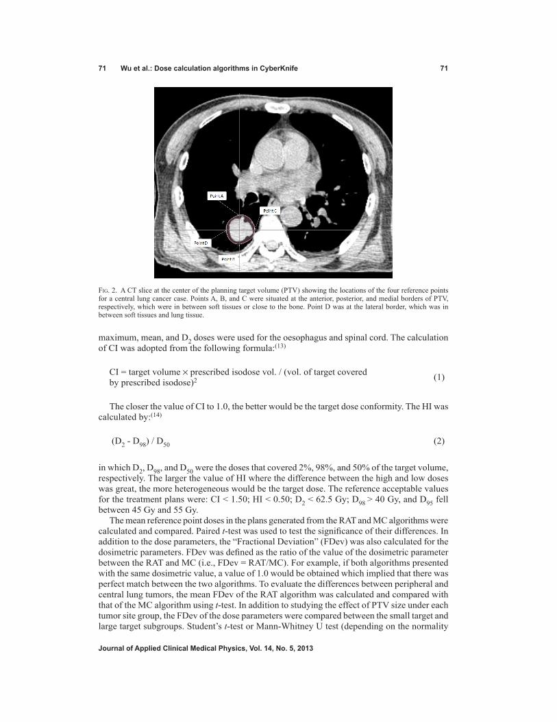
71 Wu et al.: dose calculation algorithms in CyberKnife 71
Journal of Applied Clinical Medical Physics, Vol. 14, no. 5, 2013
maximum, mean, and D2 doses were used for the oesophagus and spinal cord. The calculation of CI was adopted from the following formula:(13)
CI = target volume × prescribed isodose vol. / (vol. of target covered by prescribed isodose)2 (1)
The closer the value of CI to 1.0, the better would be the target dose conformity. The HI was calculated by:(14)
(D2 - D98) / D50 (2)
in which D2, D98, and D50 were the doses that covered 2%, 98%, and 50% of the target volume, respectively. The larger the value of HI where the difference between the high and low doses was great, the more heterogeneous would be the target dose. The reference acceptable values for the treatment plans were: CI < 1.50; HI < 0.50; D2 < 62.5 Gy; D98 > 40 Gy, and D95 fell between 45 Gy and 55 Gy.
The mean reference point doses in the plans generated from the RAT and MC algorithms were calculated and compared. Paired t-test was used to test the significance of their differences. In addition to the dose parameters, the “Fractional Deviation” (FDev) was also calculated for the dosimetric parameters. FDev was defined as the ratio of the value of the dosimetric parameter between the RAT and MC (i.e., FDev = RAT/MC). For example, if both algorithms presented with the same dosimetric value, a value of 1.0 would be obtained which implied that there was perfect match between the two algorithms. To evaluate the differences between peripheral and central lung tumors, the mean FDev of the RAT algorithm was calculated and compared with that of the MC algorithm using t-test. In addition to studying the effect of PTV size under each tumor site group, the FDev of the dose parameters were compared between the small target and large target subgroups. Student’s t-test or Mann-Whitney U test (depending on the normality
Fig. 2. A CT slice at the center of the planning target volume (PTV) showing the locations of the four reference points for a central lung cancer case. Points A, B, and C were situated at the anterior, posterior, and medial borders of PTV, respectively, which were in between soft tissues or close to the bone. Point D was at the lateral border, which was in between soft tissues and lung tissue.

72 Wu et al.: dose calculation algorithms in CyberKnife 72
Journal of Applied Clinical Medical Physics, Vol. 14, no. 5, 2013
of the data) was used to test the significance of their differences. The hypothesis for the paired t-test or Mann-Whitney U test was that the values of the dosimetric parameters obtained from MC were significantly different from those of the RAT. In addition, the calculation time was recorded using a stopwatch, and the mean calculation time was compared between the two algorithms. Paired t-test was used to test the significance of the difference.
III. RESuLTS
There were 12 and five cases belonging to the small target and large target subgroup, respec-tively, in the peripheral lung cases, and eight cases in both subgroups in the central lung cases. With regard to the reference point doses of in all the 33 cases, the RAT algorithm produced dose values of 10.9%–13.1% higher than that of the MC algorithm, with all the differences reached statistical significance (p < 0.05) (Table 1). The RAT algorithm also produced sig-nificantly higher PTV doses, but lower CI and HI. In addition, the mean calculation time for MC algorithm was 44.6 ± 31.9 minutes, which was significantly longer than that of the RAT algorithm (4.8 ± 2.8 minutes, p < 0.001).
A. Peripheral lung casesThe RAT algorithm produced dose values of about 15% higher in all the reference points when compared with the MC algorithm, with the differences of Point A and C reaching significance (p = 0.039 and 0.041, respectively) (Table 2). For the PTV, MC algorithm produced significantly larger CI and HI values when compared to that of the RAT algorithm. The RAT algorithm dem-onstrated greater values in the other dose parameters, with the D95 and D98 reaching statistical significance (p = 0.015 and 0.011, respectively). There was no significant difference in the ipsilateral lung dose between the two algorithms, although the values of RAT algorithm were slightly higher. The average DVHs of the PTV and OARs are shown in Fig. 3. When comparing between the small target and large target subgroups, the FDev values of all the reference point doses and dose parameters were greater in the small target subgroup, in which the differences of Point D dose, CI, D95, and D98 were significant.
Table 1. Dosimetric comparison between Ray Tracing and Fast Monte Carlo algorithms at the reference points in the SBRT of all lung cancer cases (n = 33) using CyberKnife.
RAT MC Paired t-test Mean ± SD Mean ± SD p-value
Reference Points Point A (Gy) 50.2±10.4 43.63±9.0 0.007 Point B (Gy) 51.5±10.8 45.89±10.3 0.034 Point C (Gy) 50.5±10.9 44.78±9.4 0.027 Point D (Gy) 52.3±11.3 45.58±10.8 0.016PTV CI 1.22±0.05 1.39±0.38 0.013 HI 0.25±0.05 0.34±0.08 0.001 D2 (Gy) 62.5±10.2 58.5±9.3 0.101 D95 (Gy) 50.0±9.0 42.9±6.9 0.001 D98 (Gy) 47.8±8.8 40.5±6.4 0.001
RAT = Ray Tracing algorithm; MC = Fast Monte Carlo algorithm.

73 Wu et al.: dose calculation algorithms in CyberKnife 73
Journal of Applied Clinical Medical Physics, Vol. 14, no. 5, 2013
Table 2. Dosimetric comparison between Ray Tracing and Fast Monte Carlo algorithms in the SBRT of peripheral lung cancer cases using CyberKnife.
Dose Parameters Fractional Deviation (RAT/MC) Small Large All Cases Target Target (n = 17) (n = 12) (n = 5) RAT MC t-test MWU test Mean ±SD Mean ±SD p-value Median Median p-value
Ref Points Point A (Gy) 52.1±11.2 44.4±9.6 0.039 1.20 1.12 0.226 Point B (Gy) 53.8±11.4 46.4±10.9 0.062 1.17 1.12 0.430 Point C (Gy) 52.7±13.1 43.9±10.9 0.041 1.24 1.11 0.061 Point D (Gy) 53.8±12.5 45.8±11.6 0.061 1.23 1.05 0.012PTV CI 1.21±0.06 1.50±0.41 0.007 0.82 0.96 0.008 HI 0.24±0.04 0.34±0.09 0.001 0.73 0.81 0.064 D2 (Gy) 63.0±12.9 57.0±11.8 0.167 1.14 1.04 0.113 D95 (Gy) 51.0±10.6 41.7±9.6 0.015 1.29 1.12 0.022 D98 (Gy) 48.0±10.3 39.5±9.0 0.011 1.30 1.13 0.001Ip. Lung V20 (%) 5.3±4.8 4.8±4.6 0.769 1.10 1.00 0.712 V30 (%) 2.7±2.5 2.0±2.2 0.405 1.07 1.03 0.883 Dmean (Gy) 4.6±3.0 4.4±3.0 0.854 1.05 1.04 0.970
RAT = Ray Tracing algorithm; MC = Fast Monte Carlo algorithm; MWU = Mann-Whitney U test; PTV = planning target volume; CI = Conformity Index; HI = Homogeneity Index; Ip. = Ipsilateral, Dm = mean dose.
Fig. 3. Comparison of the average dose-volume histograms (DVHs) of the PTV and OARs between RAT and MC algorithms for the CyberKnife plans of the peripheral lung tumors.
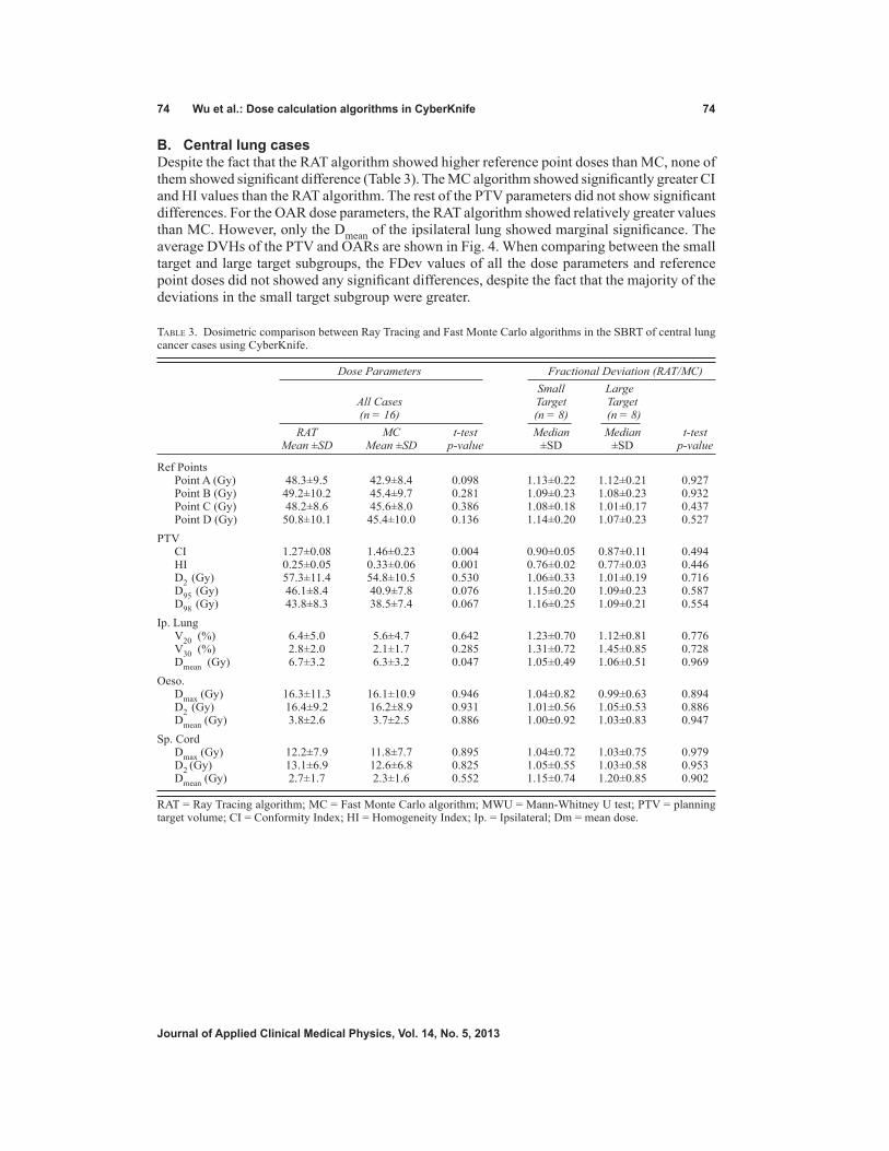
74 Wu et al.: dose calculation algorithms in CyberKnife 74
Journal of Applied Clinical Medical Physics, Vol. 14, no. 5, 2013
B. Central lung casesDespite the fact that the RAT algorithm showed higher reference point doses than MC, none of them showed significant difference (Table 3). The MC algorithm showed significantly greater CI and HI values than the RAT algorithm. The rest of the PTV parameters did not show significant differences. For the OAR dose parameters, the RAT algorithm showed relatively greater values than MC. However, only the Dmean of the ipsilateral lung showed marginal significance. The average DVHs of the PTV and OARs are shown in Fig. 4. When comparing between the small target and large target subgroups, the FDev values of all the dose parameters and reference point doses did not showed any significant differences, despite the fact that the majority of the deviations in the small target subgroup were greater.
Table 3. Dosimetric comparison between Ray Tracing and Fast Monte Carlo algorithms in the SBRT of central lung cancer cases using CyberKnife.
Dose Parameters Fractional Deviation (RAT/MC) Small Large All Cases Target Target (n = 16) (n = 8) (n = 8) RAT MC t-test Median Median t-test Mean ±SD Mean ±SD p-value ±SD ±SD p-value
Ref Points Point A (Gy) 48.3±9.5 42.9±8.4 0.098 1.13±0.22 1.12±0.21 0.927 Point B (Gy) 49.2±10.2 45.4±9.7 0.281 1.09±0.23 1.08±0.23 0.932 Point C (Gy) 48.2±8.6 45.6±8.0 0.386 1.08±0.18 1.01±0.17 0.437 Point D (Gy) 50.8±10.1 45.4±10.0 0.136 1.14±0.20 1.07±0.23 0.527PTV CI 1.27±0.08 1.46±0.23 0.004 0.90±0.05 0.87±0.11 0.494 HI 0.25±0.05 0.33±0.06 0.001 0.76±0.02 0.77±0.03 0.446 D2 (Gy) 57.3±11.4 54.8±10.5 0.530 1.06±0.33 1.01±0.19 0.716 D95 (Gy) 46.1±8.4 40.9±7.8 0.076 1.15±0.20 1.09±0.23 0.587 D98 (Gy) 43.8±8.3 38.5±7.4 0.067 1.16±0.25 1.09±0.21 0.554Ip. Lung V20 (%) 6.4±5.0 5.6±4.7 0.642 1.23±0.70 1.12±0.81 0.776 V30 (%) 2.8±2.0 2.1±1.7 0.285 1.31±0.72 1.45±0.85 0.728 Dmean (Gy) 6.7±3.2 6.3±3.2 0.047 1.05±0.49 1.06±0.51 0.969Oeso. Dmax (Gy) 16.3±11.3 16.1±10.9 0.946 1.04±0.82 0.99±0.63 0.894 D2 (Gy) 16.4±9.2 16.2±8.9 0.931 1.01±0.56 1.05±0.53 0.886 Dmean (Gy) 3.8±2.6 3.7±2.5 0.886 1.00±0.92 1.03±0.83 0.947Sp. Cord Dmax (Gy) 12.2±7.9 11.8±7.7 0.895 1.04±0.72 1.03±0.75 0.979 D2 (Gy) 13.1±6.9 12.6±6.8 0.825 1.05±0.55 1.03±0.58 0.953 Dmean (Gy) 2.7±1.7 2.3±1.6 0.552 1.15±0.74 1.20±0.85 0.902
RAT = Ray Tracing algorithm; MC = Fast Monte Carlo algorithm; MWU = Mann-Whitney U test; PTV = planning target volume; CI = Conformity Index; HI = Homogeneity Index; Ip. = Ipsilateral; Dm = mean dose.

75 Wu et al.: dose calculation algorithms in CyberKnife 75
Journal of Applied Clinical Medical Physics, Vol. 14, no. 5, 2013
C. Peripheral lung vs. central lung casesFor the reference points, the ranges of FDev were 1.18–1.21 and 1.06–1.13 for the peripheral lung and central lung, respectively (Table 4). The peripheral lung showed greater FDev values than the central lung in all reference point doses, in which the differences of Point B and C reached significance (p = 0.017 and 0.001, respectively). For the PTV dose parameters, the peripheral lung demonstrated slightly greater FDev values than that of the central lung, with only D2 showing significant difference (p = 0.026).
Fig. 4. Comparison of the average dose-volume histograms (DVHs) of the PTV and OARs between RAT and MC algorithms for the CyberKnife plans of the central lung tumors.
Table 4. Comparison of RAT-MC fractional deviations (RAT/MC) in reference point and target doses between the SBRT of peripheral lung and central lung using CyberKnife.
Fractional Deviation (RAT/MC) Peripheral Lung (n = 17) Central Lung (n = 16) t-test Mean ± SD Mean ± SD p-value
Reference Points Point A (Gy) 1.18±0.17 1.13±0.11 0.327 Point B (Gy) 1.18±0.13 1.09±0.06 0.017 Point C (Gy) 1.21±0.12 1.06±0.06 0.001 Point D (Gy) 1.20±0.22 1.13±0.15 0.297PTV CI 0.86±0.19 0.89±0.14 0.611 HI 0.76±0.18 0.77±0.14 0.733 D2 (Gy) 1.11±0.09 1.05±0.05 0.026 D95 (Gy) 1.24±0.20 1.13±0.08 0.461 D98 (Gy) 1.25±0.23 1.14±0.10 0.521
RAT = Ray Tracing algorithm; MC = Fast Monte Carlo algorithm; PTV = planning target volume; CI = Conformity Index; HI = Homogeneity Index.

76 Wu et al.: dose calculation algorithms in CyberKnife 76
Journal of Applied Clinical Medical Physics, Vol. 14, no. 5, 2013
IV. dISCuSSIon
Our study compared the MC algorithm with the RAT algorithm in the CyberKnife SBRT of NSCLC. Taking the MC algorithm as the gold standard, the differences in the calculated dose distribution between the two algorithms revealed the performance of the RAT algorithm.
In the overall comparison, the RAT algorithm was found to have overestimated the doses by 10.9%–13.1% at the reference points, which were the interfaces between the target and sur-rounding tissues. This implied that after accounting for density heterogeneity, the actual doses delivered to the patient using the RAT algorithms might range from 38.2–45.9 Gy (in 3 to 5 fractions). The finding was consistent with the finding by Sharma et al.(15) Since lung tumor was mainly surrounded by the low-density lung tissue, radiation beams usually traversed a considerable distance of low-density tissue before reaching the target; this would reduce the dose to the target due to the “build down” effect of photon beam.(7) Therefore, failure to correct this effect would lead to overestimation of the dose. Such difference found in this study illus-trated the extent of inadequacy of the RAT algorithm in the modeling of secondary electronic disequilibrium at the tumor–lung tissue interface.(16)
A. Peripheral lung casesAn average of about 15% overestimation of the reference point doses was observed in the RAT algorithm. This indicated that the RAT algorithm was less capable of handling such anatomical condition. The situation was worse in Points A and C, because most of the radiation beams were directed from the anterior directions in SBRT of lung cases; the beams would have travelled a longer path of low-density lung tissue before reaching these points. This posed a problem to the RAT algorithm. Similarly, this was also the main cause leading to the relative large differences of the PTV dose between the two algorithms. It should be noted that using the MC algorithm, the target conformity and homogeneity were deteriorated from the original plan due to a more accurate modeling of secondary electronic disequilibrium at the tumor–lung tissue interface leading to a broadened beam penumbra.(9) However, since such effect was not present in the ipslateral lung, no significant difference was seen between the two algorithms in this OAR.
Comparing the two target size subgroups, smaller targets demonstrated greater dose differ-ences (FDev values) in the PTV dose parameters between the two algorithms. This echoed the report from Haedinger et al.,(16) which stated that small targets might lead to insufficient dose to the target using the correction-based algorithm.
B. Central lung casesAlthough similar patterns of dosimetric outcome were observed in the central lung cases as in the peripheral lung cases, the differences between the two algorithms were less obvious. Furthermore, the effect of target size was also not significant, as none of the FDev values demonstrated significant differences. Since the central tumor was commonly surrounded by soft tissues, the chance for FDev values to be subjected to extreme tissue density changes, such as in the tumor–lung tissue interface, would be lower. As a result, the magnitude of second-ary electronic disequilibrium was smaller. Since such condition was less difficult for the RAT algorithm, the gap between the two algorithms was smaller.
C. Peripheral lung vs. central lung casesIn the peripheral lung cases, many of the radiation beams had to pass through a larger lung volume before reaching the target and a greater discrepancy in the calculated dose by the RAT algorithm that the central lung target would be expected. This was reflected in the greater FDev values of the peripheral lung group. Since in the central lung cases, Points B and C were sur-rounded by less volume of lung tissues than in the case of the peripheral lung cases (Figs. 1 and 2), therefore more obvious differences in FDev values between the two groups were observed. For the same reason, the FDev values of the PTV dose parameters for the peripheral lung were

77 Wu et al.: dose calculation algorithms in CyberKnife 77
Journal of Applied Clinical Medical Physics, Vol. 14, no. 5, 2013
also greater than that of the central lung cases, though only the difference of the D2 value was statistically significant. Our result was in line with another similar study by van der Voort van Zyp et al.(11) on NSCLC, but comparing equivalent path-length algorithm with MC in linear accelerator. They reported that there was an increased in dose inhomogeneity in peripheral tumors when compared with central tumors, and recommended a different prescription for different tumor size.
We assumed that the MC Algorithm used with 1% uncertainty level was the gold standard in radiotherapy dose calculation. In the treatment planning of CyberKnife, if the RAT algorithm could produce comparable dosimetric outcome as the MC algorithm, it would be welcome by the department, as its expected shorter computation time would bring about better economical value. In our study, the RAT algorithm was in general inferior to the MC algorithm, in which the target dose was usually overestimated. This implied that the actual dose delivered to the target was lower than the prescribed dose, leading to an increase risk of local recurrence. The RAT algorithm would not be recommended for SBRT of peripheral lung tumors regardless of the target size, as its dose deviations were significantly different from the MC algorithm. However, the RAT algorithm could be considered for large central lung tumors because its performance was comparable to the MC algorithm with a much shortened dose computation time.
V. ConCLuSIonS
In the radiotherapy of NSCLC using CyberKnife, the RAT algorithm was not able predict the dose distribution as accurately as the MC algorithms. A larger difference between the two algorithms was found in the treatment of small peripheral tumors than large central tumors.
REFEREnCES
1. Vahdat S, Oermann EK, Collins SP, P et al. CyberKnife radiosurgery for inoperable stage IA non-small cell lung cancer: 18F-fluorodeoxyglucose positron emission tomography/computerized tomography serial tumor response assessment. J Hematol Oncol. 2010;3:6.
2. Brown WT, Wu X, Fayad F, et al. Application of robotic stereotactic radiotherapy to peripheral stage I non-small cell lung cancer with curative intent. Clin Oncol. 2009;21(8):623–31.
3. Collins BT, Vahdat S, Erickson K, et al. Radical cyberknife radiosurgery with tumor tracking: an effective treat-ment for inoperable small peripheral stage I nom-small cell lung cancer. J Hematol Oncol 2009;2:1.
4. van der Voort van Zyp NC, Prvost J, Hoogeman MS, et al. Stereotactic radiotherapy with real-time tumor tracking for non-small cell lung cancer: clinical outcome. Radiother Oncol. 2009;91(3):296–300.
5. Timmerman R, McGarry R, Yiannoutsos C, et al. Excessive toxicity when treating central tumors in a phase II study of stereotactic body radiation therapy for medically inoperable early-stage lung cancer. J Clin Oncol. 2006;24(30):4833–39.
6. Biswas T, Holland B, Rosenman J, Podder T. Lung SBRT using Cyberknife: technique and treatment outcome [abstract]. Med Phys. 2012;39(6):3801.
7. American Association of Physicists in Medicine (AAPM), Radiation Therapy Committee, Task Group No. 65. Tissue inhomogeneity corrections for megavoltage photon beams. AAPM Report 85. Madison, WI: Medical Physics Publishing; 2004.
8. Srivastava RP, Olteanu A, Ebongue AN, Bekaert B, De Wagter C. Output measurement for small field photon beams in a sandwiched phantom. In: dossel O and Schlegel WC, editors. IFMBE Proceedings 2009. New York: Springer; 2009:601–03.
9. Wilcox EE, Dasakalov GM, Lincolon H, Shumway RC, Kaplan BM, Colasanto JM. Comparison of planned dose distributions calculated by Monte Carlo and Ray-Trace algorithms for the treatment of lung tumors with cyberknife: a preliminary study in 33 patients. Int J Radiat Oncol, Biol Phys. 2010;77(1):277–84.
10. Radiation Therapy Oncology Group. A phase II trial of stereotactic body radiation therapy in the treatment of patient with medically inoperable stage I/II non-small cell lung cancer. RTOG 0236. Philadelphia, PA: RTOG; 2009.
11. van der Voort van Zyp NC, Hoogeman MS, van de Water S, et al. Clinical introduction of Monte Carlo treat-ment planning: a different prescription dose for non-small cell lung cancer according to tumor location and size. Radiother Oncol. 2010;96(1):55–60.
12. Ma C, Li J, Deng J, Fan J. Investigation of fast Monte Carlo dose calculation for Cyberknife SRS/STR treatment planning [abstract]. Med Phys. 2007;34(6):2589.

78 Wu et al.: dose calculation algorithms in CyberKnife 78
Journal of Applied Clinical Medical Physics, Vol. 14, no. 5, 2013
13. van’t Riet A, Mak AC, Moerland MA, Elders LH, van der Zee W. A conformation number to quantify the degree of conformality in brachytherapy and external beam irradiation: application to the prostate. Int J Radiat Oncol Biol Phys. 1997;37(3):731–36.
14. ICRU. Prescribing, recording, and reporting photon-beam intensity-modulated radiation therapy (IMRT). ICRU Report 83. J ICRU. 2010;10(1).
15. Sharma SC, Ott JT, Williams JB, Dickow D. Clinical implications of adopting Monte Carlo treatment planning for CyberKnife. J Appl Clin Med Phys. 2010;11(1):3142.
16. Haedinger U, Krieger T, Flentje M, Wulf J. Influence of calculation model on dose distribution in stereotactic radiotherapy for pulmonary targets. Int J Radiat Oncol Biol Phys. 2005;61(1):239–49.

a Corresponding author: Siyong Kim, 4500 San Pablo Rd., Jacksonville, FL 32224, USA; phone: (904) 953-8259; fax: (904) 953-1010; email: [email protected]
Negative margin technique — a novel planning strategy to improve dose conformation in SBRT using dynamic conformal arc delivery
Siyong Kim,1a Taeho Kim,1,2 Stephen J. Ko,1 Christopher Serago,1 Ashley A. Smith,1 Laura A. Vallow,1 Jennifer L. Peterson,1 and Rena Lee2 Department of Radiation Oncology,1 Mayo Clinic, Jacksonville, FL, USA; Department of Radiation Oncology,2 Ewha Womans University, Seoul, [email protected]
Received 8 November, 2012; accepted 22 April, 2013
The purpose of this study was to introduce a planning strategy for dynamic confor-mal arc therapy (DCAT), named negative margin technique (NMT), and evaluate its dosimetric gain in lung stereotactic body radiation therapy (SBRT). In DCAT, the field aperture is continuously conformed to the planning target volume (PTV) with an aperture margin (AM) to compensate for the penumbra effect with gantry rotation. It is a common belief the AM should be positive (or at least ‘zero’). However, the radial penumbra width becomes significantly wider because of continuously overlapped beams in arc delivery. Therefore, we hypothesize if the ‘negative margin’ is applied in the radial direction, it would improve the PTV dose conformation while reducing normal tissue dose. For verification, trial plans were made using the NMT and compared with ‘zero margin (ZM)’ plans for five lung SBRT cases representing different situations depending on the location of the PTV and organs at risk. All plans met 95% PTV coverage with the prescription dose and spared the spinal cord below the tolerance. Two conventional conformation indices (the ratio of prescription isodose volume to the PTV (CI100) and the ratio of 50% prescription isodose volume to the PTV (CI50)) and a modified conformation index were investigated. The maximum dose at 2 cm from the PTV (Dmax-2cm) and the percent of lung volume receiving 20 Gy (V20) were also evaluated. Another plan-ning simulation was performed with a total of ten randomly selected lung SBRT cases to mimic actual practice. In this simulation, optimization with ZM was first performed and further optimization using the NMT was processed for cases that could not meet a goal of CI100 = 1.2 with the ZM optimization. In all cases, both the CI100 and CI50 values were significantly reduced (overall, 9.4% ± 4.1% and 5.9% ± 3.1% for CI100 and CI50, respectively). The modified conformation index values also showed similar improvement (overall, 10.1% ± 5.7% increase). Reduction of Dmax-2cm was also observed in all cases (4.5% ± 2.2%). V20 values decreased in all cases but one (5.7% ± 3.9%, excluding the increased case). In the random group simulation, it was possible to achieve the goal with just one NMT trial for five out of six cases that did not meet the goal in the ZM optimization. Interestingly, however, one case needed as many as six iterations to get the CI100 = 1.2 goal. The NMT turned out to be an effective planning strategy that could bring significant improvement of dose conformation. The NMT can be easily implemented in most clinics with no prerequisite.
PACS number: 87.55.D-
Key words: field aperture margin, negative margin, dynamic conformal arc therapy, lung SBRT
JOURNAL OF APPLIED CLINICAL MEDICAL PHYSICS, VOLUME 14, NUMBER 5, 2013
79 79

80 Kim et al.: Negative margin technique 80
Journal of Applied Clinical Medical Physics, Vol. 14, No. 5, 2013
I. INTRODUCTION
For the improvement of local control in small lesions in certain disease sites such as lung and liver, stereotactic body radiation therapy (SBRT) has been applied.(1-3) Because of significantly larger fractional dose, SBRT requires high dose conformality, as well as precise beam delivery, and various beam delivery and planning techniques have been developed.(4-6) Dynamic con-formal arc therapy (DCAT), developed mainly for stereotactic radiosurgery (SRS), is capable of delivering conformal doses with efficiency for SBRT.(6-8)
Due to a significantly high ablative dose prescription compared to conventional therapy, dose conformation is extremely important in SBRT. For example, the Radiation Oncology Therapy Group (RTOG) 0915 protocol, a randomized phase II study comparing two SBRT fractionation schedules for medically inoperable patients with stage I peripheral non-small cell lung cancer, requires a conformality index of smaller than 1.2 for the planning target volume (PTV).(1)
In this study, we introduce a planning strategy of DCAT for the improvement of dose con-formation, and evaluate its dosimetric gain in lung SBRT.
II. MATERIALS AND METHODS
A. Theory/hypothesisWhile the gantry rotates, in DCAT, the field aperture is continuously conformed to the planning target volume (PTV) in the beam’s eye view (BEV) with an aperture margin (AM) to compensate for the penumbra effect. It is a common belief that the field aperture should be larger than or at least the same as the PTV to get adequate target coverage. However, it has been observed that the radial penumbra in the arc plane becomes significantly wider due to the continuous dose overlapping nature of the arc delivery. Thus, it may be hypothesized that if negative margin (NM) in the radial direction is allowed contrary to the common belief, it would improve the PTV dose conformation while reducing the surrounding normal tissue dose. This newly introduced method is named ‘negative margin technique (NMT)’.
B. Study with a systematic group
B.1 Planning trials For the verification of the hypothesis, planning simulation was performed with a total of five actual lung SBRT cases. Each of the five cases was systematically chosen to represent a dis-tinguishable clinical situation, as shown in Fig. 1:
Case 1 — the PTV was relatively small and located with enough distance from each organ at risk (OAR); Case 2 — the PTV was relatively large and located in a moderate distance from the spinal cord; Case 3 — the PTV was located close to the spinal cord; Case 4 — the PTV was located at lateral–posterior corner with relatively close distance to the skin; and Case 5 — the PTV was located too laterally, thus only partial arc was available due to col-lision problem.
For each case, two plans, one with ‘zero aperture margin’ (noted as ZM) and the other using negative aperture margin technique (noted as NMT), were obtained. Planning was carried out using a Philips Pinnacle (ver. 9) treatment planning system (TPS) (Philips Healthcare, Andover, MA) with a 6 MV photon beam of a Varian IX machine. Dose calculation was performed with heterogeneity correction using convolution–superposition algorithm which showed minimal perturbation in small photon fields.(9) All plans met two major planning objects — covering at least 95% of the PTV with the prescription dose (48 Gy in 4 fractions), and sparing the spinal cord below the tolerance (volumes receiving 20.8 and 13.6 Gy or more should be less than 0.35 and 1.2 cc, respectively). Each PTV was obtained by adding 5 mm margin all around

81 Kim et al.: Negative margin technique 81
Journal of Applied Clinical Medical Physics, Vol. 14, No. 5, 2013
to its corresponding full-breathing cycle-based internal target volume (ITV). Information on internal breathing motion was obtained from a 10-phase–based 4D CT, while dose calculation was made on a free-breathing CT dataset.
Depending on the situation, it is necessary to assign a nonuniform aperture margin around the PTV. However, the version of Pinnacle TPS used did not support assigning a nonuniform aperture margin. Thus, instead of entering aperture margin values, a pseudovolume (called pseudo-PTV), initially generated by copying the PTV, was modified in six different directions (i.e., anterior, posterior, right, left, superior, and inferior direction) as needed, then the field aperture was conformed to the pseudo-PTV.
As implied before, when DCAT is used within an axial coplane, dose penumbra in both the superior and inferior directions is steep and a positive aperture margin is necessary, as in the conventional approach. In this study, about 2 to 4 mm positive aperture margin was used in superior and inferior directions, while negative aperture margins were applied to other direc-tions (i.e., anterior, posterior, right, and left direction). The amount of negative margin varied case to case. Clockwise rotation of gantry when seen from the table side was used for all arc beams. Gantry angle is 0° when it is heading toward the floor.
B.2 EvaluationTwo conventional conformation indices (CIs), the ratio of prescription isodose volume to the PTV (CI100) and the ratio of 50% prescription isodose volume to the PTV (CI50), were investigated. As described by RTOG,(10) an ideal dose conformation makes a CI100 equal to 1. When the irradiated volume is larger than the target volume, CI100 is greater than 1, indicating inclusion of surrounding normal tissue within the volume having at least the prescription dose.
Fig. 1. Axial plane at the isocenter level for each case in the systematic group: PTVs are in orange color wash (displayed in scales close each other for easy comparison).

82 Kim et al.: Negative margin technique 82
Journal of Applied Clinical Medical Physics, Vol. 14, No. 5, 2013
If the target volume is only partially irradiated to the necessary dose (i.e., prescription dose), it makes a CI100 smaller than 1.
In addition to the conventional conformation indices, a modified conformation index (noted as M-CI100 in this study) suggested by Paddick(11) was also investigated. M-CI100 is defined as:
TVPIV2 / (TV × PIV) (1)
where TV is target volume, PIV is prescription isodose volume, and TVPIV is the overlapped volume between TV and PIV (i.e., target volume having prescription dose). As can be noted in the equation, M-CI100 is either smaller or equal to 1. While CI100 is subject to giving a false perfect score depending on the situation, M-CI100 is not.
Besides conformation indices, the maximum dose at 2 cm from the PTV as a percentage of the prescription dose (Dmax-2cm) and the percent of lung volume receiving 20 Gy or more (V20) were evaluated.
C. Study with a random groupTo closely mimic actual practice, another planning simulation was performed with a total of ten randomly selected lung SBRT cases. In this simulation, optimization with zero aperture margin in radial direction was first performed and evaluated based on CI100. A goal of CI100 = 1.2 is routinely used in our clinic. Thus, if a case met this goal with zero aperture margin, no further optimization was processed. For other cases, however, optimization was continued until the goal was achieved and the number of iterations was recorded.
III. RESULTS
A. Systematic group study Compared to the conventional zero margin plans, both CI100 and CI50 values decreased signifi-cantly in the NMT plans for all five cases (overall, 9.4% ± 4.1% reduction in CI100 and 5.9% ± 3.1% reduction in CI50). M-CI100 values also showed similar improvement (overall, 10.1% ± 5.7% increase). Note improvement means reduction in conventional CIs and increase in M-CI. Table 1 summarizes detailed CI values for all cases. Other important parameters such as PTV volume, percent prescription isodose line chosen, beam arc ranges, and aperture margins used are also shown in the Table 1. In Case 1, for example, the PTV was 20.5 cm3, the prescription isodose lines were 80% and 76% for the ZM and NMT, respectively; the aperture margins in the longitudinal direction were +3 mm for both the superior and inferior directions; the aperture margins in the radial direction were -1 mm for all directions (i.e., anterior, posterior, right, and left direction) for the full range of angles (i.e., from 181° to 180° clockwise); CI100 values were 1.27 in the ZM plan and 1.16 in the NMT plan; the change of CI100 from the ZM to the NMT was -8.7%; CI50 values were 4.67 in the ZM plan and 4.21 in the NMT plan; the change of CI50 from the ZM to the NMT was -9.9%; M-CI100 values were 0.72 in the ZM plan and 0.78 in the NMT plan; and the change of M-CI100 from the ZM to the NMT was 8.2%.
As shown in Table 1, for Cases 2 and 3 where the spinal cord was of concern, multiple partial arcs were used instead of one full arc. With multiple partial arcs it was possible to bet-ter optimize dose distributions by assigning different beam weights for different partial arcs (mainly to avoid irradiating the spinal cord over the tolerance). Having different beam weights for different partial arcs caused less symmetric dose distributions in the radial direction in the ZM plan. For this reason, negative aperture margins were applied for only two partial arcs (e.g., 261°–330° arc and 81°–150° arc in Case 2), and margins were nonuniform (e.g., -2 mm in anterior direction and -3 mm in posterior direction in Case 2) in the NMT plan.

83 Kim et al.: Negative margin technique 83
Journal of Applied Clinical Medical Physics, Vol. 14, No. 5, 2013
Because the PTV was located close to the skin in Case 4, a noticeably asym-metrical dose distribution with hotter dose skewed toward the skin was obtained in the ZM plan. To compensate for such severe dose asymme-try, positive aperture margins (+3 mm) were used for both the anterior and right direc-tions, while negative aperture margins (-3 mm) were chosen for both the posterior and left directions, which brought significant gain in CI100 (i.e., 15.2% reduction from the ZM to NMT plan).
In Case 5, the PTV was placed too laterally to have a full arc without collision. Thus, a partial arc beam from 181° to 90° clockwise was used and it caused more gen-erous dose distributions in the anterior and right direc-tions, which then resulted in necessitating negative mar-gins in both the anterior and right directions.
Comparisons of Dmax-2cm (the maximum dose at 2 cm from the PTV as a percentage of the prescription dose) and V20 (the percent of lung volume receiving 20 Gy) between the ZM and NMT plan were sum-marized in Table 2. As shown, reduction in the Dmax-2cm was observed in all cases (aver-age -4.5% ± 2.2% change). Except in Case 4, the values of V20 also decreased (aver-age -5.7% ± 3.9% change, excluding Case 4). In Case 4, the PTV was located close to the posterior side of the lung and the dose distribution was tilted towards the back in the ZM plan. With the margins applied in the NMT plan, the dose distribution was moved Ta
ble
1.
Com
paris
on o
f con
form
atio
n in
dice
s be
twee
n co
nven
tiona
l zer
o m
argi
n (Z
M) p
lans
and
neg
ativ
e m
argi
n te
chni
que
(NM
T) p
lans
for a
ll te
sted
cas
es in
the
syst
emat
ic g
roup
.
%
Px
AM
ARC
AM
PTV
Isod
ose
SI
Angl
e AP
RL
CI 10
0 C
I 100
ΔCI 10
0 C
I 50
CI 50
ΔC
I 50
M-C
I 100
M-C
I 100
ΔM-C
I 100
Cas
e (c
m3 )
(Z
M/N
MT)
(m
m)
(°)
(mm
) (Z
M)
(NM
T)
(%)
(ZM
) (N
MT)
(%
) (Z
M)
(NM
T)
(%)
1
20.5
80
/76
S&I+
3 18
1-18
0 -1
1.
27
1.16
-8
.7
4.67
4.
21
-9.9
0.
72
0.78
8.
2
2 52
.3
76/7
5 S&
I+2
181-
260
NC
1.
18
1.13
-4
.2
4.54
4.
40
-3.1
0.
78
0.80
3.
3
261-
330
A-2
, P-3
33
1-80
N
C
81-1
50
A-2
, P-3
15
1-18
0 N
C
3
45.4
80
/77
S&I+
2 18
1-22
0 N
C
1.34
1.
19
-11.
2 5.
11
4.73
-7
.4
0.68
0.
77
13.5
22
1-31
6 A
-2, P
-5
317-
46
NC
47
-136
A
-2, P
-5
137-
180
NC
4
30.8
72
.5/7
7 S+
3,
181-
180
A&
R+3
, 1.
38
1.17
-1
5.2
5.35
5.
21
-2.6
0.
66
0.77
17
.8
I+
4
P&L-
3
5 32
.3
80/8
0 S&
I+3
181-
90
A-1
, R-1
1.
30
1.20
-7
.7
4.81
4.
49
-6.7
0.
71
0.76
7.
5
M
ean
-9.4
Mea
n -5
.9
M
ean
10.1
SD
4.1
SD
3.
1
SD
5.7
%Px
: = p
erce
nt p
resc
riptio
n; A
M =
ape
rture
mar
gin;
S, I
, A, P
, R, a
nd L
= s
uper
ior,
infe
rior,
ante
rior,
post
erio
r, rig
ht, a
nd le
ft di
rect
ions
(e.g
., A
-2 in
dica
tes
-2 m
m m
argi
n in
ant
erio
r di
rect
ion)
; NC
= n
o m
argi
n ch
ange
; ΔC
I = c
hang
e of
CI f
rom
ZM
to N
MT
in %
= [C
I(N
MT)
/ C
I(ZM
) - 1
] × 1
00.
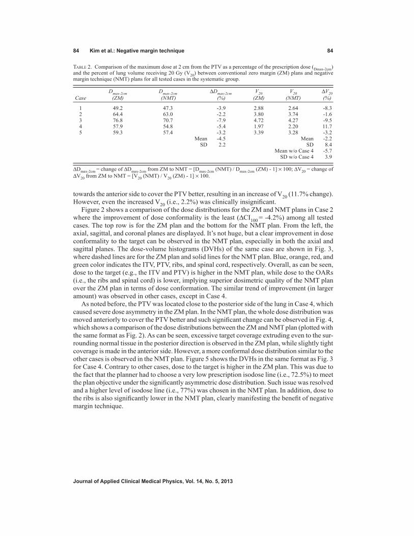
84 Kim et al.: Negative margin technique 84
Journal of Applied Clinical Medical Physics, Vol. 14, No. 5, 2013
towards the anterior side to cover the PTV better, resulting in an increase of V20 (11.7% change). However, even the increased V20 (i.e., 2.2%) was clinically insignificant.
Figure 2 shows a comparison of the dose distributions for the ZM and NMT plans in Case 2 where the improvement of dose conformality is the least (ΔCI100 = -4.2%) among all tested cases. The top row is for the ZM plan and the bottom for the NMT plan. From the left, the axial, sagittal, and coronal planes are displayed. It’s not huge, but a clear improvement in dose conformality to the target can be observed in the NMT plan, especially in both the axial and sagittal planes. The dose-volume histograms (DVHs) of the same case are shown in Fig. 3, where dashed lines are for the ZM plan and solid lines for the NMT plan. Blue, orange, red, and green color indicates the ITV, PTV, ribs, and spinal cord, respectively. Overall, as can be seen, dose to the target (e.g., the ITV and PTV) is higher in the NMT plan, while dose to the OARs (i.e., the ribs and spinal cord) is lower, implying superior dosimetric quality of the NMT plan over the ZM plan in terms of dose conformation. The similar trend of improvement (in larger amount) was observed in other cases, except in Case 4.
As noted before, the PTV was located close to the posterior side of the lung in Case 4, which caused severe dose asymmetry in the ZM plan. In the NMT plan, the whole dose distribution was moved anteriorly to cover the PTV better and such significant change can be observed in Fig. 4, which shows a comparison of the dose distributions between the ZM and NMT plan (plotted with the same format as Fig. 2). As can be seen, excessive target coverage extruding even to the sur-rounding normal tissue in the posterior direction is observed in the ZM plan, while slightly tight coverage is made in the anterior side. However, a more conformal dose distribution similar to the other cases is observed in the NMT plan. Figure 5 shows the DVHs in the same format as Fig. 3 for Case 4. Contrary to other cases, dose to the target is higher in the ZM plan. This was due to the fact that the planner had to choose a very low prescription isodose line (i.e., 72.5%) to meet the plan objective under the significantly asymmetric dose distribution. Such issue was resolved and a higher level of isodose line (i.e., 77%) was chosen in the NMT plan. In addition, dose to the ribs is also significantly lower in the NMT plan, clearly manifesting the benefit of negative margin technique.
Table 2. Comparison of the maximum dose at 2 cm from the PTV as a percentage of the prescription dose (Dmax-2cm) and the percent of lung volume receiving 20 Gy (V20) between conventional zero margin (ZM) plans and negative margin technique (NMT) plans for all tested cases in the systematic group.
Dmax-2cm Dmax-2cm ΔDmax-2cm V20 V20 ΔV20 Case (ZM) (NMT) (%) (ZM) (NMT) (%)
1 49.2 47.3 -3.9 2.88 2.64 -8.3 2 64.4 63.0 -2.2 3.80 3.74 -1.6 3 76.8 70.7 -7.9 4.72 4.27 -9.5 4 57.9 54.8 -5.4 1.97 2.20 11.7 5 59.3 57.4 -3.2 3.39 3.28 -3.2 Mean -4.5 Mean -2.2 SD 2.2 SD 8.4 Mean w/o Case 4 -5.7 SD w/o Case 4 3.9
ΔDmax-2cm = change of ΔDmax-2cm from ZM to NMT = [Dmax-2cm (NMT) / Dmax-2cm (ZM) - 1] × 100; ΔV20 = change ofΔV20 from ZM to NMT = [V20 (NMT) / V20 (ZM) - 1] × 100.

85 Kim et al.: Negative margin technique 85
Journal of Applied Clinical Medical Physics, Vol. 14, No. 5, 2013
Fig. 2. Dose distribution comparison between the ZM and NMT plan for Case 2: ZM plan (top), NMT plan (bottom), axial plane (left), sagittal plane (middle), and coronal plane (right).
Fig. 3. Dose-volume histogram (DVH) comparison between the ZM and NMT plan for Case 2: ZM plan (dashed line), NMT plan (solid line), ITV (blue), PTV (orange), ribs (red), and spinal cord (green).

86 Kim et al.: Negative margin technique 86
Journal of Applied Clinical Medical Physics, Vol. 14, No. 5, 2013
B. Random group studySix out of ten cases showed CI100 of higher than 1.2 in the ZM optimization. Further optimization using the NMT for these cases brought significant improvement (overall, 8.9% ± 2.3% reduc-tion in CI100, 8.7% ± 2.4% reduction in CI50, and 9.8% ± 2.1% increase in M-CI100), resulting in the achievement of planning goal of CI100 = 1.2 or less for every case. Detailed values are summarized in Table 3. To be distinguished from the systematic group, cases in the random group are noted with letter ‘R’ in the front of each case number (e.g., Case R1, Case R2, and so on). Regarding the number of iterations, it was possible to achieve the goal with just one
Fig. 4. Dose distribution comparison between the ZM and NMT plan for Case 4: ZM plan (top), NMT plan (bottom), axial plane (left), sagittal plane (middle), and coronal plane (right).
Fig. 5. Dose-volume histogram (DVH) comparison between the ZM and NMT plan for Case 4: ZM plan (dashed line), NMT plan (solid line), ITV (blue), PTV (orange), ribs (red), and spinal cord (green).
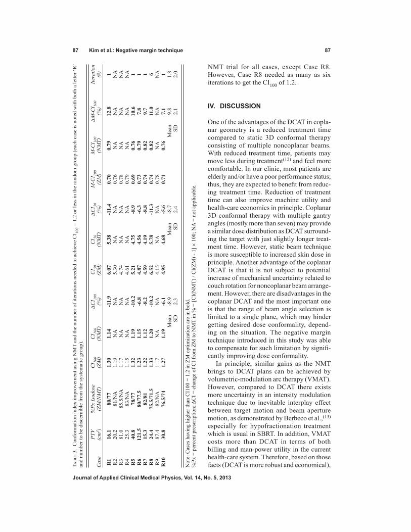
87 Kim et al.: Negative margin technique 87
Journal of Applied Clinical Medical Physics, Vol. 14, No. 5, 2013
NMT trial for all cases, except Case R8. However, Case R8 needed as many as six iterations to get the CI100 of 1.2.
IV. DISCUSSION
One of the advantages of the DCAT in copla-nar geometry is a reduced treatment time compared to static 3D conformal therapy consisting of multiple noncoplanar beams. With reduced treatment time, patients may move less during treatment(12) and feel more comfortable. In our clinic, most patients are elderly and/or have a poor performance status; thus, they are expected to benefit from reduc-ing treatment time. Reduction of treatment time can also improve machine utility and health-care economics in principle. Coplanar 3D conformal therapy with multiple gantry angles (mostly more than seven) may provide a similar dose distribution as DCAT surround-ing the target with just slightly longer treat-ment time. However, static beam technique is more susceptible to increased skin dose in principle. Another advantage of the coplanar DCAT is that it is not subject to potential increase of mechanical uncertainty related to couch rotation for noncoplanar beam arrange-ment. However, there are disadvantages in the coplanar DCAT and the most important one is that the range of beam angle selection is limited to a single plane, which may hinder getting desired dose conformality, depend-ing on the situation. The negative margin technique introduced in this study was able to compensate for such limitation by signifi-cantly improving dose conformality.
In principle, similar gains as the NMT brings to DCAT plans can be achieved by volumetric-modulation arc therapy (VMAT). However, compared to DCAT there exists more uncertainty in an intensity modulation technique due to inevitable interplay effect between target motion and beam aperture motion, as demonstrated by Berbeco et al.,(13) especially for hypofractionation treatment which is usual in SBRT. In addition, VMAT costs more than DCAT in terms of both billing and man-power utility in the current health-care system. Therefore, based on those facts (DCAT is more robust and economical), Ta
ble
3.
Con
form
atio
n in
dex
impr
ovem
ent u
sing
NM
T an
d th
e nu
mbe
r of i
tera
tions
nee
ded
to a
chie
ve C
I 100 =
1.2
or l
ess i
n th
e ra
ndom
gro
up (e
ach
case
is n
oted
with
bot
h a
lette
r ‘R
’ an
d nu
mbe
r to
be d
isce
rnib
le fr
om th
e sy
stem
atic
gro
up).
PTV
%Px
Isod
ose
CI 10
0 C
I 100
ΔCI 10
0 C
I 50
CI 50
ΔC
I 50
M-C
I 100
M-C
I 100
ΔM-C
I 100
Itera
tion
Cas
e (c
m3 )
(Z
M/N
MT)
(Z
M)
(NM
T)
(%)
(ZM
) (N
MT)
(%
) (Z
M)
(NM
T)
(%)
(#)
R1
16.1
80
/77
1.30
1.
14
-11.
9 6.
07
5.38
-1
1.4
0.70
0.
79
12.8
1
R2
20.2
81
/NA
1.
19
NA
N
A
5.30
N
A
NA
0.
76
NA
N
A
NA
R3
81.0
85
.5/N
A
1.17
N
A
NA
4.
74
NA
N
A
0.78
N
A
NA
N
A R
4 25
.3
83/N
A
1.15
N
A
NA
4.
61
NA
N
A
0.79
N
A
NA
N
A R
5 40
.8
78/7
7 1.
32
1.19
-1
0.2
5.21
4.
75
-8.9
0.
69
0.76
10
.6
1 R
6 12
1.5
80/7
7.5
1.23
1.
15
-6.8
4.
87
4.56
-6
.3
0.73
0.
79
7.8
1 R
7 15
.3
82/8
1 1.
22
1.12
-8
.2
4.59
4.
19
-8.8
0.
74
0.82
9.
7 1
R8
24.4
75
.5/7
1.5
1.33
1.
20
-10.
2 6.
52
5.78
-1
1.3
0.74
0.
82
11.0
6
R9
87.4
82
/NA
1.
17
NA
N
A
4.15
N
A
NA
0.
78
NA
N
A
NA
R10
30
.8
76.5
/74
1.27
1.
19
-6.1
4.
95
4.68
-5
.6
0.71
0.
76
7.1
1
Mea
n -8
.9
M
ean
-8.7
Mea
n 9.
8 1.
8
SD
2.3
SD
2.
4
SD
2.1
2.0
Not
e: C
ases
hav
ing
high
er th
an C
I100
= 1
.2 in
ZM
opt
imiz
atio
n ar
e in
bol
d.%
Px =
per
cent
pre
scrip
tion;
ΔC
I = c
hang
e of
CI f
rom
ZM
to N
MT
in %
= [C
I(N
MT)
/ C
I(ZM
) - 1
] × 1
00; N
A =
not
app
licab
le.

88 Kim et al.: Negative margin technique 88
Journal of Applied Clinical Medical Physics, Vol. 14, No. 5, 2013
DCAT is the first choice in our clinic, and VMAT is used only when it is difficult to obtain an acceptable dose distribution with DCAT, as in the case when either multiple targets exist closely or critical organs are located too close to the target.
When a target is located very close to skin, there is a high probability that dose to the skin exceeds the accepted tolerance, increasing the risk of skin complications. As illustrated in Case 4, the NMT enables manipulating the dose distribution in a certain degree to reduce skin dose in such cases.
The PTV, in Case 5, was placed laterally and it was not possible to have a full arc due to the issue of gantry collision with either the patient or table when the isocenter was at the center of the PTV. In such a situation, an alternative solution is to set up the isocenter centrally outside the PTV and use off-axis fields to get full arc geometry without collision problems. However, in principle, this approach is more susceptible to mechanical uncertainties, such as collimator angle and gantry angle error. Thus, treating with partial arc geometry with the isocenter at the PTV center is preferred in our clinic. It is inevitable to have more asymmetric dose distribution in that case than usual, and the NMT can mitigate such an issue, as demonstrated in this study.
It is generally true that beam margin is correlated with dose heterogeneity. More specifically, lower prescription isodose line (PIL) is expected with tighter margin. Except Case 4, which represents a totally different situation from others as explained before, selected PILs in the NMT plans are lower than those in the ZM plans for all cases. However, as can be seen in Tables 1 and 3, the amount of PIL change does not seem significant (i.e., less than 5%) compared to that of conformation index change (i.e., reaching up to over 12%). We believe this is related to the shape of dose distribution (dose gradient) near the point where the PIL is selected. The PILs in this study are at about 80% for the ZM plans where dose gradient is not that steep. Thus, margin change in few mm would not cause significant PIL change which is directly related to dose heterogeneity.
The negative margin needed in Case 3 reached up to 5 mm in posterior direction for two partial arcs. Although it seems quite large, the target can still get necessary dose because the rest of the arcs bring enough dose in posterior direction.
During the plan optimization process in this study, the negative margins were determined by trial and error. Thus, the margin values might not be fully optimized. It is considered that more optimal values could be obtained if more time and endeavor were invested. Based on the random group study, it seems possible to get satisfactory optimization with reasonable effort for most cases. Compared to other cases in the random group study, however, Case R8 required significantly larger number of iterations (six vs. one) to achieve the CI100 = 1.2 goal. It is interesting to note that for Case R8, the CI100 values were 1.33, 1.25, 1.23, 1.21, 1.21, 1.21, and 1.2 in the order of iteration from zero to six. This implies there are chances, although not frequent, that a huge effort is necessary to get fine conformation improvement. We believe if the NMT is incorporated into a treatment planning system as a plan optimization algorithm, it would provide more consistent and optimal margins, as well as make the process simpler. Dose conformation with DCAT is heavily related to the dose gradient in the penumbra region, especially at the isodose point chosen for dose prescription. Dose gradient is a function of many parameters such as beam quality, field size, and irradiation material. Thus, it would be useful to evaluate dose distribution characteristics according to such parameters to properly develop the NMT optimization algorithm for a TPS.
In this study, we mainly focused on lung SBRT but, in principle, the NMT can be applied to some other sites such as liver. However, both the amount of negative margin needed and the gain realized may be different, and independent analyses would be needed for the expansion of NMT to other disease sites.

89 Kim et al.: Negative margin technique 89
Journal of Applied Clinical Medical Physics, Vol. 14, No. 5, 2013
V. CONCLUSIONS
Compared to the conventional zero margin plans, the level of dose conformality was significantly better in the negative margin technique plans. Based on the results of plan simulations, NMT is an effective planning strategy that could bring significant improvement of dose conformation. When the NMT is applied, planners are expected to achieve plan objectives with coplanar field(s) only, which then would result in efficient beam delivery with less mechanical uncertainty. The NMT can be easily implemented in most clinics with no prerequisite.
ACKNOWLEDGMENTS
This study was in part supported by the Industrial Strategic Technology Development Program (10035527) funded by the Ministry of Knowledge Economy (MKE, Korea).
REFERENCES
1. Videtic GM, Signh AK, Chang JY, et al. A randomized phase II study comparing 2 stereotactic body radiation therapy (SBRT) schedules for medically inoperable patients with stage I peripheral non-small cell lung cancer. Radiation Therapy Oncology Group 0915. Philadelphia, PA: ACR; 2009.
2. Timmerman R, Abdulrahman R, Kavanagh BD, Meyer JL. Lung cancer: a model for implementing stereotactic body radiation therapy into practice. In: Meyer JL, Kavanagh BD, Purdy JA, Timmerman R, editors. IMRT, IGRT, SBRT – advanced in the treatment planning and delivery of radiotherapy. Basel: Karger; 2007:367–85.
3. Rusthoven KE, Kavanagh BD, Cardenes H, et al. Multi-institutional phase I/II trial of stereotactic body radiation therapy for liver metastases. J Clin Oncol. 2009;27(10):1572–78.
4. Solberg TD, Boedeker KL, Fogg R, Selch MT, DeSalles AA. Dynamic arc radiosurgery field shaping: a comparison with static field conformal and noncoplanar circular arcs. Int J Radiat Oncol Biol Phys. 2001;49(5):1481–91.
5. Buyyounouski MK, Balter P, Lewis B, et al. Stereotactic body radiotherapy for early-stage non-small-cell lung can-cer: report of the ASTRO Emerging Technology Committee. Int J Radiat Oncol Biol Phys. 2010;78(1):3–10.
6. Benedict SH, Yenice KM, Followill D, et al. Stereotactic body radiation therapy: the report of AAPM Task Group 101. Med Phys. 2010;37(8):4078–101.
7. Takeda A, Kunieda E, Sanuki N, et al. Dose distribution analysis in stereotactic body radiotherapy using dynamic conformal multiple arc therapy. Int J Radiat Oncol Biol Phys. 2009;74(2):363–69.
8. Wiggenraad RG, Petoukhova AL, Versluis L, van Santvoort JP. Stereotactic radiotherapy of intracranial tumors: a comparison of intensity-modulated radiotherapy and dynamic conformal arc. Int J Radiat Oncol Biol Phys. 2009;74(4):1018–26.
9. Jones AO and Das IJ. Comparison of inhomogeneity correction algorithms in small photon fields. Med Phys. 2005;32(3):766–76.
10. Shaw E, Kline R, Gillin M, et al. Radiation Therapy Oncology Group: radiosurgery quality assurance guidelines. Int J Radiat Oncol Biol Phys. 1993;27(5):1231–39.
11. Paddick I. A simple scoring ratio to index the conformity of radiosurgical treatment plans. Technical note. J Neurosurg. 2000;93(Suppl 3):219–22.
12. Kim S, Akpati HC, Kielbasa JE, et al. Evaluation of intrafraction patient movement for CNS and head and neck IMRT. Med Phys. 2004;31(3):500–06.
13. Berbeco RI, Pope CJ, Jiang SB. Measurement of the interplay effect in lung IMRT treatment using EDR2 films. J Appl Clin Med Phys. 2006;7(4):33–42.

a Corresponding author: Asghar Hadadi, Department of Medical Radiation Engineering, Science and Research Branch, Islamic Azad University, P.O. Box 14515-775, Tehran, Iran; phone: (+98) 021-44817170; fax: (+98) 021-44817175; email: [email protected]
Monte Carlo characterization of biocompatible beta-emitting 90Y glass seed incorporated with the radionuclide 153Sm as a SPECT marker for brachytherapy applications
Asghar Hadadi,1a Mahdi Sadeghi,2 Dariush Sardari,1 Alireza Khanchi,3 Alireza Shirazi4Department of Medical Radiation Engineering,1 Science and Research Branch, Islamic Azad University, Tehran, Iran; Agricultural, Medical and Industrial Research School,2 Nuclear Science and Technology Research Institute, Karaj, Iran; Nuclear Science and Technology Research Institute,3 Tehran, Iran; Department of Biophysics,4 Faculty of Medicine, Medical Sciences, University of Tehran, Tehran, [email protected]
Received 26 November, 2012; accepted 1 April, 2013
A glass seed consisting of the β–-emitting radionuclide 90Y incorporated with radionuclide 153Sm as SPECT marker is proposed for potential application in brachytherapy in order to reduce the undesirable dose to healthy adjacent organs. The aim of this work is to determine the dosimetric characteristics, as suggested in the AAPM TG-60/TG-149 reports, for this seed using Monte Carlo simulation. Monte Carlo codes MCNP5, EGSnrc, and FLUKA were used to calculate the absorbed dose distribution around the seed. Dosimetric parameters, such as refer-ence absorbed dose rate, radial dose function, and one-dimensional (1D) and two-dimensional (2D) anisotropy functions, were obtained. The computational results from these three codes are in agreement within 5.4% difference on average. The absorbed dose rate at the reference point was estimated to be 5.01 cGy h-1 μCi-1 and self absorption of YAS glass seed amounted to 30.51%. The results showed that, with thermal neutron bombardment of 5 hours in a typical flux, sufficient activity for applications in brachytherapy may be achieved. With a 5 mCi initial activity, the total dose of a YAS glass seed was estimated to be 1.38 Gy at 1.0 cm from the seed center. Comparing with gamma emitting seeds, the 90Y seed could reduce undesir-able doses to adjacent organs, because of the rapid dose falloff of beta ray. Because of the high R90 value of 5.5 mm, fewer number of 90Y seeds will be required for an interstitial brachytherapy treatment using permanent implant, in comparison with other beta-emitting seeds. The results would be helpful in the development of the radioactive implants using 90Y glass seeds for the brachytherapy treatment.
PACS numbers: 87.53.Jw, 87.56.bg
Key words: brachytherapy, dosimetry, YAS glass, TG-60 protocol, Monte Carlo simulation
I. InTroduCTIon
Beta-ray seeds offer several advantages over photon seeds. Beta particles have short ranges; therefore, they can give a potentially lower dose to adjacent critical organs. They are shielded easily, lowering extra dose to medical staff as well as the patient. Beta-ray seeds such as 90Sr/90Y, 90Y, 32P, 106Ru/106Rh are widely and routinely used for brachytherapy applications
JournAL oF APPLIEd CLInICAL MEdICAL PHYSICS, VoLuME 14, nuMBEr 5, 2013
90 90

91 Hadadi et al.: MC characterization of 90Y glass seed 91
Journal of Applied Clinical Medical Physics, Vol. 14, no. 5, 2013
including intravascular brachytherapy (IVBT) and treatment of pterygia, choroid melanomas, and retinoblastomas.(1)
Several factors, such as the type and energy of radiation and half-life, must be considered for radionuclide selection in permanent interstitial brachytherapy of selected localized tumors. Table 1 presents the comparison of the properties of several beta emitters.(2) The radionuclide 90Y is an ideal medical isotope with very interesting therapeutic features. This radionuclide is a pure beta emitter with high endpoint energy 2.284 MeV and half-life 64.0 h. The maximum range of the 90Y beta radiation in water is 11 mm, and 90% of the emitted energy is absorbed within a sphere of water with a radius of 5.3 mm.(3) For the first time in 1956, Mallard et al.(4) raised the idea of using the radionuclide 90Y for treatment of pituitary tumors. Since then, 90Y pituitary implants were used in the 1960s and 1970s as one of the first-line treatments for pituitary tumors in many endocrine centers.(5)
In the field of cancer radiotherapy, rare earth aluminosilicate (REAS) glasses have been used as radioactive material vehicles because they can contain large amounts of beta-emitting rare earth isotopes (e.g., 90Y, 166Ho, 153Sm and 165Dy from 25 to 70 wt%). In this type of application, glasses should be biocompatible, nontoxic, and chemically insoluble, to prevent radioactivity leakage within the in vivo treatment site. REAS glasses are chemically durable and biologically inert in vivo.(6,7) Another advantage of this glass is that the desired nonradioactive isotope is incorporated within the glass structure and activated in situ by neutron bombardment to form the beta-emitting isotope and, hence, handling of radioactive materials during the manufacturing process is avoided.(8) Yttrium aluminosilicate (YAS) glasses are of most interest among others because of their applicability in interstitial brachytherapy. YAS glasses, in the form of micro-spheres or seeds, have received attention in the treatments of liver cancer, rheumatoid arthritis, and prostate tumors.(9) In 1987, Hyatt and Day(8) studied ten YAS glasses, made by traditional high temperature melting, with yttria content varying from 25 to 55 wt%. They found that the VHN for YAS glasses is high compared to other glasses, so these glasses should display good resistance against abrasion. These glasses were also found to have very high chemical durabil-ity in distilled water. In 1993, Erbe and Day(10) first reported that 17Y2O3–19Al2O3–64SiO2 (mol %) (YAS) glass had most chemical durability in distilled water at 37°C and, based on their excellent chemical durability, YAS glass microspheres of 20–30 μm diameter were suitable for in vivo applications. Besides, In 1994, White and Day(6) studied YAS glasses in the form of microspheres (20 to 40 μm in diameter) and seeds (with dimensions approximately 0.8 mm diameter and 5 mm length) to deliver large doses to sites inside the body.
Currently, bioactive and biodegradable glasses, made by sol–gel technique, are also of interest for interstitial brachytherapy. Roberto et al.(11,12) introduced the bioactive SiO2-CaO-152Sm2O3 glasses produced by the sol-gel process for prostate cancer treatment. These glasses may be activated by neutron bombardment to form the beta-emitting 153Sm isotope. Preliminary
Table 1. Properties of several beta-emitting radionuclides.
Average Abundance Thermal Neutron Maximum Energy Energy of Parent γ Emissions Cross Section of Radionuclide Half-life (MeV) (MeV) (%) (keV) Parent (b)a
90Y 64.0 h 2.284 (100%) 0.934 100 Brems 1.28 90Sr 29.1 y 0.546 (100%) 0.196 - Brems - 32P 14.3 d 1.710 (100%) 0.695 100 Brems 0.172 186Re 90.6 h 1.076 (73.0%) 0.35 37.4 137 (8.65%) 112 188Re 17.0 h 2.119 (71.6%) 0.764 62.6 155 (14.9%) 76.4 153Sm 46.7 h 0.817 (21.0%) 0.228 26.75 103 (28.3%) 206 142Pr 19.1 h 2.159 (96.3%) 0.809 100 1580 (3.7%) 11.5 177Lu 6.71 d 0.497 (78.6%) 0.133 2.59 208 (11.0%) 2090 166Ho 26.8 h 1.856 (51.0%) 0.667 100 80.6 (6.2%) 64.7
a Mughabghab SF(30)

92 Hadadi et al.: MC characterization of 90Y glass seed 92
Journal of Applied Clinical Medical Physics, Vol. 14, no. 5, 2013
studies for the implant of biodegradable radioactive 153Sm seeds in the liver and brain have been previously published.(13,14,15) Other investigators synthesized two sets of ceramic seeds by the sol–gel technique with Si-Ca-Sm and Si-Ca-Ho incorporating natural samarium and holmium elements for use in brachytherapy.(16,17,18,19)
The updated American Association of Physicists in Medicine (AAPM) TG-43U1 report rec-ommended a dosimetry protocol for interstitial brachytherapy seeds.(20) TG-43U1 parameters are explicitly for low-energy photon-emitting brachytherapy seeds, such as 125I and 103Pd, and beta-emitting seeds were not included. The AAPM TG-60/TG-149 reports addressed intravas-cular brachytherapy physics and included the recommendation of dosimetry of beta emitters, such as 90Sr/90Y and 32P.(21,22)
The aim of the present work is to determine the dosimetric characteristics of β–-emitting YAS glass seed incorporated with 153Sm as a SPECT marker for potential use in permanent or temporary interstitial implant for treating suitable tumors. The AAPM TG-60/TG-149 dosimetric parameters, such as reference absorbed dose rate, radial dose function, and one-dimensional (1D) and two-dimensional (2D) anisotropy functions, were calculated in water for a cylindrical seed using the Monte Carlo method based on the MCNP5, EGSnrc, and FLUKA radiation transport code systems. The dose rates in different radial distances from the seed and various angles, as well as isodose curves were derived. Moreover, the selfabsorption of the seed, R90 value, and the activity of seed in thermal neutron flux for various bombardment times were evaluated. In order to investigate the viability of producing seed, the trial fabrication of the YAS glass seed with the isotope 152Sm incorporated by sol–gel technique was evaluated.
II. MATErIALS And METHodS
A. Seed descriptionThe YAS glass seed is a cylinder 4.5 mm long and 0.8 mm diameter, the same as the typical 125I seeds. The glass is composed of 43.2% Y, 7.9% Al, 14% Si, 34.7% O, and 0.2% 152Sm (in wt %) with a density of 3.8 g/cm3. The glass with composition of Y2O3: 55%, Al2O3: 15%, and SiO2: 30%, that has been used in the work by Hyatt and Day,(8) is transparent with a slight yellow tint. The used chemical precursors were TEOS (Si(OC2H5)4, Merck, 98%), yttrium nitrate hexahydrate (Y(NO3)3 . 6H2O, Daejung, > 99.9%), aluminium nitrate nonahydrate (Al(NO3)3 . 9H2O, Merck, ≥ 98.5%), and enriched samarium oxide (152Sm2O3, ISOTEC, 98.7%). The de-ionized water and ethanol (Carlo Erba, 99.8%) as a solvent, nitric acid (2N) as an acid catalyst, and formamide (HCONH2, Merck, ≥ 99.0%) as a modifier, were used in the sol–gel preparation. All reagents were of analytic grade. The samarium was introduced dur-ing the sol-gel synthesis as a solution prepared by solubilization of the oxide with nitric acid. After mixing the above composites and homogenization (stirred for 30 minutes on a magnetic agitator heated at 60ºC), the mixture was placed in Teflon molds, with cylindrical punctures, so that they could acquire the desired seed format. When the solution appeared like a gel, it was dried in an electric oven at 110ºC, about 20 hours. Then, the dried seeds were removed from the molds and put in a ceramic crucible and subjected to heat treatments carried out at 500ºC for 1 hour and at 1000ºC for 24 hours. Because the thermal treatment is carried out at high temperature, the glass-forming elements are closely bound together; therefore, after implantation, they will not be released into the body. However, these elements are not harmful to the body. In order to assess the leakage of seed, the active 90Y glass seed was kept inside the distilled water, then the water was analyzed for a period of two weeks. After this period, there was no evidence of leakage in water. Figure 1 illustrates the sample of desired glass seed. Because of high density of YAS glass, a radio-opaque marker is not necessary; however, the 103 keV gamma ray emitted by 153Sm can be detected by a gamma camera.(23) Also, cladding or encapsulation is not required because the seed is nonreactive in water or tissue. The YAS glass seed may be activated by neutron bombardment in a thermal neutron flux density typical

93 Hadadi et al.: MC characterization of 90Y glass seed 93
Journal of Applied Clinical Medical Physics, Vol. 14, no. 5, 2013
of research reactors to form the 90Y and 153Sm radionuclides. Table 2 presents several radio-nuclides that are made during activation of YAS glass seed.(2) The activity of seed in thermal neutron flux of 3 × 1013 cm-2s-1 was calculated using FLUKA code. The activities of 90Y, 31Si, 28Al, and 153Sm isotopes and total activity of seed were calculated to be 5.750, 0.208, 11.894, 0.95, and 17.852 mCi after 5 hours irradiation, respectively. Due to low thermal neutron cross section, the production of 90mY and 19O were ignored. With a cooling time of 13 hours after the irradiation end (approximately five times the half-life of 31Si), the activities of 31Si and 28Al isotopes are not considered to be significant. At this time, the activity of 90Y isotope is approximately 5 mCi, equivalent to values used in brachytherapy, and the activity of 153Sm isotope is approximately 0.8 mCi, enough to be suitable for SPECT imaging. Three YAS glass seeds containing 152Sm were irradiated for 30 hours in the 5 MW research reactor TRR in an irradiation position, with thermal and epithermal neutron fluxes of 2.3 × 10¹² n.cm-2s-1 and 2.5 × 10¹⁰ n.cm-2s-1, respectively. After 5 hours cooling time, these seeds were placed with 1 cm distance from each other into the cylindrical water phantom with a diameter of 15 cm and a length of 20 cm. Figure 2 illustrates the SPECT image of these seeds that was obtained using DST-XL dual-head gamma camera system. It should be noted that with increase in thermal neutron flux density or yttrium and samarium content in the seed, the required irradiation time for desired activity is decreased. Also, the seed could be used for an HDR treatment if a high neutron flux reactor having more than 1015 cm-2s-1 becomes available.
Fig. 1. YAS glass seed incorporated with 152Sm obtained by the sol-gel process.
Table 2. Radionuclides from neutron activation of YAS glass.
Thermal Neutron Cross Radionuclide Section of Parent (b) Half-life Radiation Yield
90Y 1.28a 64.1 h β 2.284 MeV 100% 90mY 0.001b 3.19 h γ 480 keV 90.0%
153Sm 206.00a 46.7 h β 0.817 MeV 21.0% γ 103 keV 28.3%
31Si 0.107a 2.62 h β 1.492 MeV 99.9% γ 1.27 MeV 0.07%
28Al 0.231a 2.24 m β 2.864 MeV 100%
γ 1.78 MeV 100%
19O 0.00016a 26.9 s β 4.819 MeV 56.1% γ 1.36 MeV 50.3%
a Mughabghab SF(30)b Handbook on nuclear activation cross-sections(31)

94 Hadadi et al.: MC characterization of 90Y glass seed 94
Journal of Applied Clinical Medical Physics, Vol. 14, no. 5, 2013
B. dose calculation formalismFor deriving dosimetric parameters, the dose calculation formalism for beta seeds recommended by the AAPM TG-60/TG-149 reports was adopted in this work. For a beta-emitting seed, the reports recommend, for reference absorbed dose rate in water w (r0, Θ0), the reference point should be r0 = 2 mm and Θ0 = 90° on the transverse axis. A line-source approximation, with the same effective length of the seed, for geometry function GL(r,Θ) was assumed when it was used to derive radial dose function gL(r) and the anisotropy function F(r,Θ).
C. Monte Carlo simulationAn important advantage of Monte Carlo (MC) simulations is that the dose distribution can be calculated with high spatial precision. Due to the extremely large dose gradient around the beta-ray sources, it is difficult to obtain accurate dose distribution experimentally. Therefore, MC simulation is widely used as an alternative means to determine the dose distribution around the radioactive seeds for therapeutic purposes. A variety of well-validated general-purpose MC codes are currently available for brachytherapy dosimetry. In this study, the MCNP5 (version 1.5.1) Los Alamos National Laboratory, Los Alamos, NM), EGSnrc (version 4 2.3.2) (NRC, Ottawa, Canada), and FLUKA (version 2011.2.8) (www.fluka.org ) Monte Carlo codes were used to calculate the quantitative dosimetric parameters of the 90Y seed.
MCNP is a general-purpose, time-dependent Monte Carlo transport code. It can be used for neutron, photon, electron, or coupled neutron/photon/electron transport. It can model an arbitrary three-dimensional geometry and various source types such as point, surface, and volume with user-defined source spectrum. The photon energy regime is from 1 keV to 100 GeV, and the electron energy regime is from 1 KeV to 1 GeV. The electron physics in MCNP is essentially that of the ITS3.0 and uses the Goudsmit–Saunderson multiple scattering theory. The user creates an input file that is subsequently read by MCNP. The user can instruct MCNP to make various tallies related to particle current, particle flux, and energy deposition. A pulse height tally F8 provides the energy distribution of pulses created in a detector by radiation.(24)
The EGSnrc system of computer codes is a general purpose package for the Monte Carlo simulation of the coupled transport of electrons and photons in an arbitrary geometry. The dynamic range of charged particle kinetic energies begins from a few tens of keV up to a few hundred GeV, and dynamic range of photon energies lies between 1 keV and several hundred
Fig. 2. The SPECT image of three YAS glass seeds that were placed into the cylindrical water phantom.

95 Hadadi et al.: MC characterization of 90Y glass seed 95
Journal of Applied Clinical Medical Physics, Vol. 14, no. 5, 2013
GeV. This code includes a variety of general purpose user RZ codes for cylindrical geometry problems such as DOSRZnrc, FLURZnrc, CAVRZnrc, and SPRRZnrc. The user code DOSRZnrc calculates absorbed dose in any cylindrical geometry. The RZ codes systematically make use of 15 different types of source geometries including parallel beam source, point source, circular source, and cylindrical source. The EGSnrc code adopts the new multiple scattering model PRESTA-II that has been developed by Kawrakow et al.,(25) which makes a significant advance in the science of electron transport.
FLUKA is a multipurpose Monte Carlo code which can simulate with high accuracy the interaction and propagation in matter of about 60 different particles. The dynamic ranges of photon and electron energies go from 1 keV to thousands of TeV. Moreover, time evolution and tracking of emitted radiation from unstable residual nuclei can be performed online by this code. Decay scoring is one of the valuable features of this code that has been used in this study. FLUKA can handle even very complex geometries, using an improved version of the well-known Combinatorial Geometry (CG) package. The various source types such as point, spherical shell, cylindrical shell, Cartesian shell, and spherical surface can be defined in this code. The electron transport in FLUKA is based on its code EMF. This code adopts Ferrari-Sala multiple scattering model, which is essentially based on Moliere’s theory.(26)
The input parameters commonly used such as the materials and geometry of source and the cutoff energies for electron and photon were exactly the same for these codes. A cylindrical volume source, with composition that is shown in Table 3, was modeled. The radionuclide was assumed to be uniformly distributed in the source. The beta spectrum used for the MC simulations is provided in Fig. 3.(2) The dosimetric data in the scoring zones were calculated at radial distances from the source from 1 to 10 mm in 0.5 mm increments, and over angles ranging from 0° to 90° in 10° increments.
MCNP5 simulations were carried out with the center of the cylindrical source placed at the center of a 20 cm radius spherical water phantom, approximating a semi-infinite water phantom, allowing for full electron scattering conditions in the region of interest. The scoring geometry is composed of an array of ring shaped volumes. These volumes are defined by the intersection of a series of concentric spherical shells with a series of concentric cones, both originating at the center of the cylindrical source. The thicknesses of spherical shells are 0.1 mm, and the angular aperture difference of two adjacent concentric cones defining the cell is 2°. The *F8 tally was used to score the energy deposited in the scoring cells around the source. Dose was calculated with *F8 tally divided by mass of scoring cells. Mode P E was used with default modeling of bremsstrahlung. MCPLIB04 and el03 cross-sectional libraries were used for the electron and photon-coupled transport. The cutoff energies for electron and photon were taken as CUT:E = 0.04 MeV and CUT:P = 0.01 MeV, and the number of electron substeps per energy step, ESTEP value, was set as built–in default adjusted for all materials. Moreover, an ITS-style energy-indexing algorithm was used for a more accurate sampling energy straggling. This algorithm serves to reduce the frequent repetition of unwanted imposition of linear interpolation on partial steps, and to allow more balance among excursions above and below the energy groups from which the Landau sampling was made.(24)
Table 3. Composition of YAS glass seed.
Element Weight (%) Mass in Seed (mg)
Y 43.2 3.722 O 34.7 2.994 Si 14.0 1.203 Al 7.9 0.679 152Sm 0.2 0.02 Total 100 8.618

96 Hadadi et al.: MC characterization of 90Y glass seed 96
Journal of Applied Clinical Medical Physics, Vol. 14, no. 5, 2013
EGSnrc and FLUKA simulations were carried out with the center of the cylindrical source placed at the center of a cylindrical water phantom with a radius of 20 cm and a length of 40 cm. DOSRZnrc user code, in case of EGSnrc, and USRBIN card in case of FLUKA, were used to score the dose in the scoring zones around the source. A set of thin, short cylindrical shell segments, concentric about the long axis of source, was adopted as scoring zones. In our calculations, the radial thickness of the cylindrical shell segments was taken as 0.1 mm and their length was 0.2 mm. The cutoff energies for electron and photon were identical to that of the MCNP5 code and were taken as AE = ECUT = 0.551 MeV and AP = PCUT = 0.01 MeV for both EGSnrc and FLUKA codes. The maximum fractional energy loss in an electron step, ESTEPE value for EGSnrc, and WHAT (2) in EMFFIX card for FLUKA, was set at 0.07. In FLUKA simulations, instead of using beta spectrum that is shown in Fig. 3, the SDUM parameter in BEAM card was taken as ISOTOPE and option HI-PROPErt was set for 90Y and 153Sm radionuclides.
Monte Carlo simulations were carried out on a personal computer with an Intel Core i7-3.5 GHz CPU (Intel Corporation, Santa Clara, CA) and Windows 7 (Microsoft, Redmond, WA) Ultimate OS for MCNP5 and EGSnrc codes, and Fedora 15 (Red Hat; Raleigh, NC)
Fig. 3. The beta-ray spectrum of: (a) 90Y, (b) 153Sm.
(a)
(b)

97 Hadadi et al.: MC characterization of 90Y glass seed 97
Journal of Applied Clinical Medical Physics, Vol. 14, no. 5, 2013
linux-based OS for FLUKA code. The number of source electron histories was set at 2 × 10⁸ for each simulation in order to obtain a statistical error less than 1% at the reference point.
III. rESuLTS & dISCuSSIon
A. The radial dose profile and reference dose rate Table 4 presents the radial dose rate values from MCNP5, EGSnrc, and FLUKA simulations, at different distances from center of the seed on the transverse axis. As shown in this table, the results of the three codes are in good agreement with each other. With 2 × 10⁸ histories, the relative statistical uncertainties at reference point were 0.06%, 0.07%, and 0.06% for MCNP5, EGSnrc, and FLUKA codes, respectively. Figure 4 illustrates the statistical uncertainties for these codes as a function of distance on the transverse axis. These uncertainties correspond to one standard deviation. As can be seen from Fig. 4, statistical uncertainties are less than 1% to 8.5 mm, and MCNP5 code has statistical uncertainties less than two other codes. The reference absorbed dose rates per unit activity for glass seed that are calculated using the above mentioned codes, are presented in Table 5. The average of depicted values, 5.01 cGy h-1 μCi-1, was chosen as the reference value for glass seed. The reference value for this glass seed is higher than the values of 3.30, and 2.412 cGy h-1 μCi-1, calculated for Novoste Beta-Cath 90Sr/90Y seeds, and 142Pr glass seed, respectively.(22,7) The uncertainties in this table are associated with relative statistical uncertainties of Monte Carlo simulation. The two-dimensional dose profiles from MCNP code simulation are observed in Fig. 5. In this figure, the interpolation was performed using the kriging algorithm in the SURFER program (Golden Software Inc., Golden, CO).
Table 4. Monte Carlo-calculated radial dose rate of 90Y glass seed.
Radial Distance Dose Rate (cGy/h/μCi) (mm) MCNP5 EGSnrc FLUKA
1.0 15.1808 14.8252 15.1650 1.5 8.3660 8.1798 8.3662 2.0 5.0542 4.9524 5.0244 2.5 3.2021 3.1369 3.1440 3.0 2.0809 2.0366 2.0120 3.5 1.3742 1.3373 1.2952 4.0 0.9000 0.8799 0.8346 4.5 0.5858 0.5750 0.5326 5.0 0.3784 0.3706 0.3375 5.5 0.2383 0.2331 0.2081 6.0 0.1445 0.1428 0.1256 6.5 0.0844 0.0837 0.0727 7.0 0.0470 0.0468 0.0400 7.5 0.0246 0.0246 0.0211 8.0 0.0121 0.0121 0.0104 8.5 0.0054 0.0055 0.0047 9.0 0.0022 0.0022 0.0019 9.5 0.0008 0.0008 0.0008 10.0 0.0003 0.0003 0.0003

98 Hadadi et al.: MC characterization of 90Y glass seed 98
Journal of Applied Clinical Medical Physics, Vol. 14, no. 5, 2013
Fig. 4. Relative statistical uncertainties of MCNP5, EGSnrc, and FLUKA codes as a function of distance on the transverse axis.
Fig. 5. Isodose contour map around the 90Y glass seed. The labels of the isodose lines are in units of cGy/h/μCi.
Table 5. The absorbed dose rates at the reference point in water.
ḊW (r0,θ0 ) Monte Carlo Code (cGy/h/μCi)
MCNP5 5.0542±0.0029 EGSnrc 4.9524±0.0035 FLUKA 5.0244±0.0030 Average 5.0103±0.0018

99 Hadadi et al.: MC characterization of 90Y glass seed 99
Journal of Applied Clinical Medical Physics, Vol. 14, no. 5, 2013
B. radial dose function gL(r)The radial dose function, gL(r), was defined in order to characterize the effects of absorption and scatter in the medium along the transverse axis of the seed. The values of radial dose function are calculated using MCNP5, EGSnrc, and FLUKA codes and are presented in Table 6. The gL(r) values from these codes are in good agreement with each other; the agreement between MCNP5 with EGSnrc is especially significant. A fifth-order polynomial fit of the MCNP5 radial dose function can be expressed as:
gL(r) = a0 + a1r + a2r2 + a3r
3 + a4r4 + a5r
5 (1)
where a0 = 1.02772, a1 = 0.18833, a2 = -0.13205, a3 = 0.0172, a4 = -7.31 × 10⁻⁴, and a5 = 4.06 × 10⁻⁶, and define correlation coefficient R = 0.99998.
Figure 6(a) shows a comparison of radial dose functions of 90Y glass seed, Amersham Health model 6733 125I seed,(27) and Best Medical model 2335 103Pd seed.(27) As can be seen in this logarithmical figure, the radial dose function profiles for 125I and 103Pd seeds are approximately flat to 10 mm, while that of 90Y glass seed falls off to 0.1% at the same distance. The compari-son of initial dose rate of these seeds is provided in Fig. 6(b). The air-kerma strengths, SK, for 125I and 103Pd seeds, which commonly used for prostate implants, are selected to be 0.75 U and 2 U, respectively. Also, the initial activity of 90Y seed is 1 mCi. As shown in this figure, the initial dose rate adjacent to the 90Y seed is much higher than those of 125I and 103Pd seeds, but decreases sharply to 41% of that of 125I seed at 10 mm. After 11 mm, the maximum range of 90Y beta radiation, the initial dose rate of 90Y seed is due to bremsstrahlung radiation and is significantly lower than those of 125I and 103Pd seeds. At 40 mm, the initial dose rate of 90Y seed decreases to approximately 0.3% and 0.2% those of 103Pd and 125I seeds, respectively, and therefore the absorbed dose by the healthy adjacent organs is decreased. However, it should be noted that when the effective distance of seed is so short, the seed’s ability to deliver effective dose to the whole irregular shaped tumor may be limited. In Fig. 7, the radial dose function of the 90Y glass seed is compared to those of the several beta-emitter seeds.(7,22,23,28,29) As observed in figure, the radial dose function of this seed is approximately similar to those of the 90Sr/90Y, and 142Pr seeds. Also, the decrease in radial dose function for that is slower than to those of the
Table 6. Monte Carlo-calculated radial dose function gL(r) for the 90Y glass seed.
Radial Distance gL(r)
(mm) MCNP5 EGSnrc FLUKA
1.0 1.100 1.100 1.108 1.5 1.070 1.070 1.076 2.0 1.000 1.000 1.000 2.5 0.912 0.917 0.905 3.0 0.810 0.816 0.792 3.5 0.703 0.697 0.664 4.0 0.587 0.586 0.548 4.5 0.475 0.475 0.433 5.0 0.374 0.371 0.332 5.5 0.282 0.285 0.251 6.0 0.202 0.201 0.174 6.5 0.137 0.138 0.118 7.0 0.088 0.089 0.075 7.5 0.053 0.055 0.046 8.0 0.030 0.031 0.026 8.5 0.015 0.015 0.013 9.0 0.007 0.007 0.006 9.5 0.003 0.003 0.003 10.0 0.001 0.001 0.001
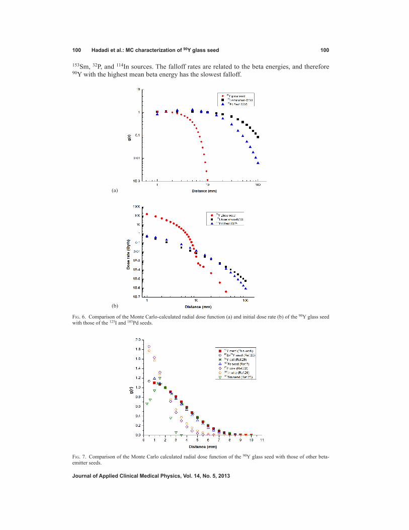
100 Hadadi et al.: MC characterization of 90Y glass seed 100
Journal of Applied Clinical Medical Physics, Vol. 14, no. 5, 2013
153Sm, 32P, and 114In sources. The falloff rates are related to the beta energies, and therefore 90Y with the highest mean beta energy has the slowest falloff.
Fig. 6. Comparison of the Monte Carlo-calculated radial dose function (a) and initial dose rate (b) of the 90Y glass seed with those of the 125I and 103Pd seeds.
(a)
(b)
Fig. 7. Comparison of the Monte Carlo calculated radial dose function of the 90Y glass seed with those of other beta-emitter seeds.

101 Hadadi et al.: MC characterization of 90Y glass seed 101
Journal of Applied Clinical Medical Physics, Vol. 14, no. 5, 2013
C. 1d and 2d anisotropy functionsThe 2D anisotropy function F(r,θ) accounts for the variation in dose distribution around the seed as a function of polar angle relative to the transverse plane. The 1D anisotropy function, ϕan(r), is identical to the anisotropy factor defined by the original TG-43 proto-col.(20) The values of the 1D and 2D anisotropy func-tions that are calculated using MCNP5 code are listed in Table 7. The maximum value of the 2D anisotropy function was calculated to be 6.785.
d. The self-absorption of the seed and r90 value
With a 64.0 h half-life, 90% of the dose from 90Y isotope is deposited in 8.86 days. Due to interseed attenuation, the part of beta energy is deposited within the seed. The self-absorption of 90Y glass seed was calculated to be 30.25% and 30.77% using EGSnrc and FLUKA codes, respectively. Therefore, the contained activity of this seed is approximately 1.4 times the apparent activity. The R90 value is defined as the radius of a sphere around the seed in water in which 90% of the output energy of seed is absorbed. The R90 value for 90Y glass seed, which was calculated using FLUKA simulation, was found to be 5.5 mm, which is in agree-ment with that found by Dezarn et al.(3)
IV. ConCLuSIonS
90Y is a pure beta-emitting isotope with interesting therapeutically features for potential use in cancer treatment. In this study, a β–-emitting YAS glass seed incorporated with 153Sm as a SPECT marker, with dimensions of 0.8 mm diameter and 4.5 mm length, is proposed for application in permanent interstitial implantation of selected localized tumors. This seed is nonreactive in the biological tissue; therefore, encapsulation is not required. The MCNP5 (version 1.5.1), EGSnrc (version 4 2.3.2), and FLUKA (version 2011.2.8) Monte Carlo codes were used to calculate the quantitative dosimetric parameters, suggested in the AAPM TG-60/TG-149 reports. The input param-eters used were exactly the same for each code, to ensure that the differences in calculated results are only due to the differences in physical modeling between these codes. The results of these codes are in good agreement with each other. The YAS glass seed has desirable dosimetric properties. The dose rate in the reference point was calculated to be 5.01 cGy h-1 μCi-1, and average of self absorption of YAS glass seed was estimated to 30.51%. The R90 value was found to Ta
ble
7. M
onte
Car
lo-c
alcu
late
d an
isot
ropy
func
tion
F(r,θ
) for
the
90Y
gla
ss s
eed.
θ
r (m
m)
(deg
) 1.
0 1.
5 2.
0 2.
5 3.
0 3.
5 4.
0 4.
5 5.
0 5.
5 6.
0 6.
5 7.
0 7.
5 8.
0 8.
5 9.
0 9.
5 10
.0
0
0.
856
0.93
9 0.
979
0.95
5 1.
036
1.09
4 1.
162
1.31
8 1.
352
1.64
5 1.
967
2.31
7 2.
774
3.86
0 5.
544
5.88
6
10
0.
948
0.94
4 0.
966
0.99
8 1.
048
1.10
2 1.
189
1.29
2 1.
422
1.62
3 1.
893
2.31
3 2.
901
3.84
1 5.
146
6.78
5
20
1.
110
1.13
3 1.
007
0.98
9 1.
005
1.03
3 1.
079
1.13
2 1.
205
1.30
2 1.
430
1.60
7 1.
854
2.18
6 2.
728
3.55
7 4.
789
5.98
2
30
1.05
1 1.
064
1.08
5 1.
048
1.03
4 1.
042
1.06
6 1.
099
1.14
1 1.
202
1.28
5 1.
398
1.54
5 1.
750
2.05
2 2.
505
3.16
9 4.
068
4.90
6
40
1.02
1 1.
045
1.06
3 1.
055
1.04
8 1.
055
1.07
1 1.
099
1.13
2 1.
180
1.25
0 1.
334
1.45
5 1.
616
1.81
0 2.
117
2.66
8 3.
313
3.91
4
50
1.01
1 1.
029
1.04
3 1.
043
1.04
2 1.
050
1.06
1 1.
084
1.10
4 1.
145
1.18
6 1.
250
1.32
8 1.
445
1.59
1 1.
805
2.10
1 2.
498
2.79
0
60
1.00
6 1.
016
1.02
5 1.
027
1.02
9 1.
034
1.04
1 1.
055
1.06
8 1.
093
1.11
5 1.
152
1.19
6 1.
267
1.35
6 1.
484
1.61
9 1.
912
1.92
0
70
1.00
3 1.
008
1.01
2 1.
011
1.01
4 1.
017
1.02
1 1.
027
1.03
3 1.
043
1.05
5 1.
077
1.09
6 1.
124
1.14
6 1.
225
1.28
3 1.
354
1.41
1
80
1.00
1 1.
002
1.00
4 1.
003
1.00
4 1.
003
1.00
5 1.
009
1.00
7 1.
010
1.01
5 1.
025
1.02
5 1.
034
1.03
9 1.
056
1.06
0 1.
090
0.94
9
90
1.00
0 1.
000
1.00
0 1.
000
1.00
0 1.
000
1.00
0 1.
000
1.00
0 1.
000
1.00
0 1.
000
1.00
0 1.
000
1.00
0 1.
000
1.00
0 1.
000
1.00
0ϕ a
n(r)
1.
107
1.34
5 1.
313
1.40
6 1.
277
1.20
8 1.
178
1.16
7 1.
165
1.17
9 1.
205
1.25
1 1.
310
1.39
9 1.
522
1.70
8 1.
987
2.37
4 2.
668

102 Hadadi et al.: MC characterization of 90Y glass seed 102
Journal of Applied Clinical Medical Physics, Vol. 14, no. 5, 2013
be 5.5 mm, equivalent to volume of approximately 0.7 cm3. Because of the high R90 value of 90Y seed, a fewer number of seeds will be required for an interstitial brachytherapy treatment using permanent implant in comparison with other beta-emitting seeds. With 5 hours for irra-diation time in thermal neutron flux of 3 × 1013 cm-2s-1 and 13 hours for cooling time, the seed activity of approximately 5 mCi may be achieve. With this initial activity, the total dose of YAS glass seed was estimated to 1.38 Gy at 1.0 cm from the seed center on the transverse axis. As shown in Fig. 2, the 103 keV gamma ray emitted from glass seed incorporated with 153Sm can be detected by a gamma camera. It should be noted that the YAS glass seed is reusable after a HDR afterloading brachytherapy route by reactivation. Also, unused seeds are reusable by reactivation. It should be considered that because of relatively short half-life of 90Y, the YAS glass seed generally has a high initial dose rate. For such a high dose rate seed, an implant other than the precise seed placement could significantly under- or overdose the target. Moreover, the process of seed production using sol-gel method is time-consuming, and due to shrinkage and deformation during the sol-gel process, the seed manufacturing is relatively difficult.
ACknowLEdgMEnTS
The authors are thankful to the Isotopes Research Group for allowing the accomplishment of this work in the scope of their professional and academic activities.
rEFErEnCES
1. Caswell RS, DeLuca PM, Seltzer SM, Wambersie A. Dosimetry of beta rays and low-energy photons for brachytherapy with sealed sources. J ICRU. 2004;4(2):5–8.
2. Radiological Toolbox, Version 2.0.0. Oak Ridge, TN: Oak Ridge National Laboratory; Available from: http://www.nrc.gov/about-nrc/regulatory/research/radiological-toolbox.html
3. Dezarn WA, Cessna JT, DeWerd LA, et al. Recommendations of the American Association of Physicists in Medicine on dosimetry, imaging, and quality assurance procedures for 90Y microsphere brachytherapy in the treatment of hepatic malignancies. Med Phys. 2011;38(8):4824–45.
4. Mallard JR, McKinnell A, Francois PE. Seeds of pure beta-ray emitter (Yttrium-90) for radiation hypophysectomy. Nature. 1956;178(4544):1240–41.
5. Jarosz JM, Malcolm PN, Cox TCS, Bingham JB. Magnetic resonance imaging features of pituitary yttrium-90 rod implantation. Clin Radiol. 1998;53(8):604–07.
6. White JE and Day DE. Rare earth aluminosilicate glasses for in vivo radiation delivery. Key Eng Mater. 1994;94-95:181–208.
7. Jung JW and Reece WD. Dosimetric characterization of 142Pr glass seeds for brachytherapy. Appl Radiat Isot. 2008;66(4):441–49.
8. Hyatt MJ and Day DE. Glass properties in the Yttria-Alumina-Silica system. J Am Ceram Soc. 1987;70(10):283–87. 9. Marchi J, Morais DS, Schneider J, Bressiani JC, Bressiani AHA. Characterization of rare earth aluminosilicate
glasses. J Non-Cryst Solids. 2005;351(10-11):863–68. 10. Erbe EM and Day DE. Chemical durability of Y2O3-Al2O3-SiO2 glasses for the in vivo delivery of beta radiation.
J Biomed Mater Res. 1993;27(10):1301–08. 11. Roberto WS, Pereira MM, Campos TPR. Structure and dosimetric analysis of biodegradable glasses for prostate
cancer treatment. Artificial Organs. 2003;27(5):432–36. 12. Roberto WS, Pereira MM, Campos TPR. Analysis of bioactive glasses obtained by sol-gel processing for radioac-
tive implants. Mater Res. 2003;6(2):123–27. 13. Campos TPR, Andrade JPL, Costa IT, Silva CHT. Study of the 153Sm seeds degradation and devaluation of the
absorbed dose in rabbit’s liver implants. Prog Nucl Energy. 2008;50:757–66. 14. Costa IT and Campos TPR. [Dosimetric response of radioactive bioglass seeds implants on rabbit’s brain] [in
Portuguese]. Matéria (Rio J.). 2007;12(3):480–86. 15. Silva GXO, Campos TPR, Siqueira SL, Maciel MB. The surgical viability and radiobiological monitoring of
brain implants of bioactive microseeds in animal model. Braz Arch Biol Technol. 2005;48:109–15. 16. Valente ES, Cuperschmid EM, de Campos TPR. Characterization of ceramic seeds with samarium-153 for use
in brachytherapy. Mater Res. 2011;14(1):21–24. 17. Valente ES and Campos TPR. Gamma spectrometry and chemical characterization of ceramic seeds with
samarium-153 and holmium-166 for brachytherapy proposal. Appl Radiat Isot. 2010;68(12):2157–62. 18. Valente ES and Campos TPR. Gamma spectrometry and chemical characterization of bioactive glass seeds with
holmium-166 for oncological implants. International Nuclear Atlantic Conference-INAC 2009, Vol.1. Rio de Janeiro: Associação Brasileira de Energia Nuclear – ABEN; 2009. p. 1–7.

103 Hadadi et al.: MC characterization of 90Y glass seed 103
Journal of Applied Clinical Medical Physics, Vol. 14, no. 5, 2013
19. Nogueira LB and Campos TPR. Nuclear characterization and investigation of radioactive bioglass seed surfaces for brachytherapy via scanning electron microscopy. J Sol-Gel Sci Technol. 2011;58:251–58.
20. Rivard MJ, Coursey BM, DeWerd LA, et al. Update of AAPM Task Group No. 43 Report: a revised AAPM protocol for brachytherapy dose calculations. Med Phys. 2004;31(3):633–74.
21. Nath R, Amols H, Coffey C, et al. Intravascular brachytherapy physics: report of the AAPM Radiation Therapy Committee Task Group No. 60. Med Phys. 1999;26(2):119–52.
22. Chiu-Tsao S, Schaart DR, Soares CG, Nath R. Dose calculation formalisms and consensus dosimetry parameters for intravascular brachytherapy dosimetry: recommendations of the AAPM Therapy Physics Committee Task Group No. 149. Med Phys. 2007;34(11):4126–57.
23. Sadeghi M, Taghdiri F, Hosseini SH, Tenreiro C. Monte Carlo calculated TG-60 dosimetry parameters for the beta-emitter 153Sm brachytherapy source. Med Phys. 2010;37(10):5370–75.
24. X-5 Monte Carlo Team. MCNP – a general Monte Carlo N-particle transport code, version 5. Los Alamos, NM: Los Alamos National Laboratory; 2008.
25. Kawrakow I, Mainegra-Hing E, Rogers DWO, Tessier F, Walters BRB. The EGSnrc code system: Monte Carlo simulation of electron and photon transport. NRCC Report PIRS-701. Ottawa: National Research Council of Canada; 2011.
26. Ferrari A, Sala PR, Fasso A, Ranft J. FLUKA: a multi-particle transport code. CERN-2005-010. Geneva: European Organization for Nuclear Research; 2011.
27. Rivard MJ, Butler WM, DeWerd LA, et al. Supplement to the 2004 update of the AAPM Task Group No. 43 Report. Med Phys. 2007;34(6):2187–205.
28. Patel NS, Chiu-Tsao S, Fan P, et al. Treatment planning dosimetric parameters for a 90Y coil source used in intravascular brachytherapy. Cardiovasc Radiat Med. 2001;2(2):83–92.
29. Schaart DR and Marijnissen JPA. A comparison of intravascular source designs based on the beta particle emitter 114mIn/114In line source versus stepping source. Cardiovasc Radiat Med. 2002;3(1):31–43.
30. Mughabghab SF. Thermal neutron capture cross sections resonance integrals and G-factors. Vienna: IAEA; 2003. 31. Handbook on nuclear activation cross-sections. IAEA Technical Reports Series No. 156. Vienna: IAEA; 1974.
a Corresponding author: Langner, Department of Radiation Medicine, Markey Cancer Center, University of Kentucky, 800 Rose St., Lexington, KY 40536-0293, USA; phone: (859) 323 9947; fax: (859) 323 4849; email: [email protected]
A feasibility study using TomoDirect for craniospinal irradiation
Ulrich W. Langner,a Janelle A. Molloy, John F. Gleason Jr., Jonathan M. FeddockDepartment of Radiation Medicine, Markey Cancer Center, University of Kentucky, Lexington, KY, [email protected]
Received 26 November, 2012; accepted 7 May, 2013
The feasibility of delivering craniospinal irradiation (CSI) with TomoDirect is investigated. A method is proposed to generate TomoDirect plans using standard three-dimensional (3D) beam arrangements on Tomotherapy with junctioning of these fields to minimize hot or cold spots at the cranial/spinal junction. These plans are evaluated and compared to a helical Tomotherapy and a three-dimensional con-formal therapy (3D CRT) plan delivered on a conventional linear accelerator (linac) for CSI. The comparison shows that a TomoDirect plan with an overlap between the cranial and spinal fields might be preferable over Tomotherapy plans because of decreased low dose to large volumes of normal tissues outside of the planning target volume (PTV). Although the TomoDirect plans were not dosimetrically superior to a 3D CRT linac plan, the patient can be easily treated in the supine position, which is often more comfortable and efficient from an anesthesia standpoint. TomoDirect plans also have only one setup position which obviates the need for matching of fields and feathering of junctions, two issues encountered with conventional 3D CRT plans. TomoDirect plans can be delivered with comparable treatment times to conventional 3D plans and in shorter times than a Tomotherapy plan. In this paper, a method is proposed for creating TomoDirect craniospinal plans, and the dosimetric consequences for choosing different planning parameters are discussed.
PACS number: 87.55.D-
Key words: TomoDirect, craniospinal irradiation
I. InTroDucTIon
Medulloblastoma is a highly malignant tumor and the second most common central nervous system neoplasm in children, accounting for approximately 15% of all pediatric brain tumors.(1,2) The current standard of care consists of maximal safe resection of the tumor, followed by cranio-spinal axis irradiation (CSI) with concurrent and adjuvant chemotherapy.(3) The most up-to-date treatment strategies result in a five-year survival rate of approximately 80% for average-risk and 70%–75% for high-risk patients, respectively.(1,3-5) Despite these relatively favorable outcomes, children suffer long-term effects from radiation therapy. The most notable include impaired neurocognitive development, hearing impairment, growth retardation, endocrine dysfunction, cataract formation, cardiomyopathy, impaired fertility, and second malignancies.(3-5) Perhaps the most significant improvements in reducing late toxicities among survivors can be attributed to lowering of the CSI dose from 36 Gy to 23.4 Gy in average-risk patients, as identified from the CCG A9961 trial(3) (see http://clinicaltrials.gov/ct2/show/NCT00002875 for more detail). High-risk patients continue to require 36 Gy. A recently closed trial (ACNS 0331) attempted to further lower the CSI dose to 18 Gy in order to improve toxicity profiles. However, as the
JournAL oF APPLIED cLInIcAL MEDIcAL PHYSIcS, VoLuME 14, nuMBEr 5, 2013
104 104

105 Langner et al.: TomoDirect cSI 105
Journal of Applied clinical Medical Physics, Vol. 14, no. 5, 2013
results are not yet mature, patterns of care data suggest that a further reduction of dose to less than 23.4 Gy may be associated with higher failure rates.
The goal of CSI is to give a homogeneous radiation dose to the entire neuraxis. This is a technically challenging problem in radiotherapy planning and delivery because of the need to irradiate a large and complex target volume uniformly, while still reducing dose to organs at risk (OARs). The majority of the previously mentioned late effects are dose and volume related; therefore, more complex radiation delivery techniques, such as intensity-modulated radiation therapy (IMRT), could be utilized to reduce OAR dose and improve the already nar-row therapeutic ratio.(2,6-11) However, separate isocenters for cranial and spinal fields remain an unavoidable problem for CSI treatments on conventional linear accelerators (both for three-dimensional conformal treatment (3D CRT) techniques, as well as IMRT techniques), such that matching of these fields and junction changes continue to be necessary. Field matching leads to dosimetric heterogeneity and uncertainty in the planning target volume (PTV), which is further complicated if an IMRT technique is used. For older children, two posterior spine fields are frequently required, necessitating additional junctions and planning complexity.
To simplify field matching during IMRT techniques, solutions were developed where the matching was done by incrementally increasing the dose for each field over a defined region, resulting in a “blending” of the dose, rather than abrupt changes.(6) The major downside is that blending the junctions on a conventional linear accelerator (linac) between multiple spinal fields will require multiple IMRT plans, which is quite labor-intensive. An alterna-tive is Tomotherapy (Accuray Inc., Sunnyvale, CA), where the radiation is delivered to the complete neuraxis in a helical fashion with one setup point, thus obviating the need for field matching.(2,7-10) Tomotherapy also allows complex modulation of dose, which can provide a conformal dose to the target volume while minimizing high-dose regions in normal tissue.
The feasibility of Tomotherapy to deliver CSI is well documented.(8,10,12) However, concerns for increased secondary malignancies due to higher integral doses, and the potential impact of prolonged sedation in the setting of longer treatment times (which can be approximately five times longer than standard 3D techniques), limits the widespread use of Tomotherapy in children.(2,6-11)
TomoDirect (Accuray Inc.) is a treatment option on a Tomotherapy unit that enables 3D CRT techniques to be used. Stationary gantry positions are utilized as the couch propagates through the gantry, with the multileaf collimator (MLC) continuously conforming to the PTV volume. Two modes are possible for TomoDirect, an IMRT mode in which modulation is manipulated during planning, and a 3D CRT mode in which the leaves conform to the PTV with limited additional modulation. The ability of Tomotherapy to treat the patient in a single continuous plan without the need to junction fields is retained, without significantly increasing the integral dose to the patient or prolonging the treatment time. This is done by generating a plan using the principles of a standard 3D CRT CSI treatment on a conventional linear accelerator (referred to hereafter as 3D CRT (linac)) to achieve the aforementioned benefits without significantly increasing the integral dose.
In this paper, we investigate the feasibility of TomoDirect treatments for CSI, using standard 3D CRT beam arrangements. The dosimetric consequences for choosing different planning parameters are also discussed. The plans generated will be compared to Tomotherapy and 3D CRT (linac) plans to examine the feasibility of a TomoDirect approach. This study was approved by an institutional review board.
II. MATErIALS AnD METHoDS
A. PatientsTomoDirect plans were retrospectively created for two previously treated patients in our clinic. The patients were selected sequentially from the most recent cases treated using Tomotherapy
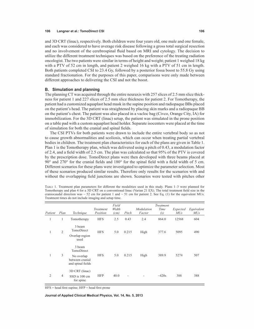
106 Langner et al.: TomoDirect cSI 106
Journal of Applied clinical Medical Physics, Vol. 14, no. 5, 2013
and 3D CRT (linac), respectively. Both children were four years old, one male and one female, and each was considered to have average risk disease following a gross total surgical resection and no involvement of the cerebrospinal fluid based on MRI and cytology. The decision to utilize the different treatment techniques was based on the preference of the treating radiation oncologist. The two patients were similar in terms of height and weight; patient 1 weighed 18 kg with a PTV of 52 cm in length, and patient 2 weighed 16 kg with a PTV of 51 cm in length. Both patients completed CSI to 23.4 Gy, followed by a posterior fossa boost to 55.8 Gy using standard fractionation. For the purposes of this paper, comparisons were only made between different approaches to delivering the CSI and not the boost.
B. Simulation and planningThe planning CT was acquired through the entire neuraxis with 257 slices of 2.5 mm slice thick-ness for patient 1 and 227 slices of 2.5 mm slice thickness for patient 2. For Tomotherapy, the patient had a customized aquaplast head mask in the supine position and radiopaque BBs placed on the patient’s head. The patient was straightened by placing skin marks and a radiopaque BB on the patient’s chest. The patient was also placed in a vacloc bag (Civco, Orange City, IA) for immobilization. For the 3D CRT (linac) setup, the patient was simulated in the prone position on a table pad with a custom aquaplast head holder. Separate isocenters were placed at the time of simulation for both the cranial and spinal fields.
The CSI PTVs for both patients were drawn to include the entire vertebral body so as not to cause growth abnormalities and scoliosis, which can occur when treating partial vertebral bodies in children. The treatment plan characteristics for each of the plans are given in Table 1. Plan 1 is the Tomotherapy plan, which was delivered using a pitch of 0.43, a modulation factor of 2.4, and a field width of 2.5 cm. The plan was calculated so that 95% of the PTV is covered by the prescription dose. TomoDirect plans were then developed with three beams placed at 90° and 270° for the cranial fields and 180° for the spinal field with a field width of 5 cm. Different scenarios for these plans were investigated to optimize the parameter selection. Most of these scenarios produced similar results. Therefore only results for the scenarios with and without the overlapping field junctions are shown. Scenarios were tested with pitches other
Table 1. Treatment plan parameters for different the modalities used in this study. Plans 1–3 were planned for Tomotherapy and plan 4 for a 3D CRT on a conventional linac (Varian 21 EX). The total treatment field size in the craniocaudal direction was ~ 52 cm for patient 1 and ~ 51 cm for patient 2. See Eq. (1) for the equivalent MUs. Treatment times do not include imaging and setup time.
Field Treatment Treatment Width Modulation Time Expected Equivalent Patient Plan Technique Position (cm) Pitch Factor (s) MUs MUs
1 1 Tomotherapy HFS 2.5 0.43 2.4 864.0 12568 604
3 beam 1 2 TomoDirect HFS 5.0 0.215 High 377.6 5095 490 Overlap region used 3 beam TomoDirect 1 3 No overlap HFS 5.0 0.215 High 389.9 5274 507 between cranial and spinal fields 3D CRT (linac) 2 4 SSD is 100 cm HFP 40.0 - - ~420s 388 388 for spine
HFS = head first supine; HFP = head first prone

107 Langner et al.: TomoDirect cSI 107
Journal of Applied clinical Medical Physics, Vol. 14, no. 5, 2013
than 0.215 (the default pitch for a 5 cm field is 0.5), high and low modulation, and normal tissue homogeneity on and off. In the TomoDirect terminology, more and less compensation refers to the amount of modulation that is allowed when the plan is calculated. More modula-tion will result in a more homogeneous dose distribution in the PTV, but will require a longer treatment time. If normal tissue homogeneity is turned on, the planning software will attempt to reduce hot spots in normal tissue outside of the PTV. It must be noted that TomoDirect plans are equivalent to 3D CRT, and modulation and homogeneity is not comparable to that achieved with Tomotherapy IMRT plans.
The TomoDirect plans were calculated so that 90% of the PTV was covered by the prescrip-tion dose. This is similar to what is done in the 3D CRT (linac) plan, where the spinal canal is covered by the 100% isodose line, but deeper parts of the vertebral body might be covered by lower isodose lines in order to reduce the maximum dose inside the PTV and minimize exit dose into anterior structures. Directional blocks were used to ensure that 90° and 270° beams were used only for the cranial fields (and not the entire neuraxis) and a posterior beam for the spinal field (see Fig. 1). Directional blocks mean that the beams cannot enter through a struc-ture that is blocked before it encounters the PTV, but it can exit after encountering the PTV.
Fig. 1. Dose distributions for TomoDirect plans with a 2.5 cm (half-field width) overlap (plan 2 – top panel) and no overlap (plan 3 – bottom panel) between the cranial and spinal fields. Directional blocks were used to ensure only opposed lateral fields for the brain, a posterior field for the spine. The directional blocks for the brain and spine are indicated by the blue and gray dotted lines. Here 23.4 Gy represents 100%.

108 Langner et al.: TomoDirect cSI 108
Journal of Applied clinical Medical Physics, Vol. 14, no. 5, 2013
An overlap region was created in the TomoDirect plans (except plan 3) by terminating these blocks for a few slices in a junction region, in order to “merge” the fields as smoothly as pos-sible. The length of this region was chosen so that the dose distribution of each field matches at ~ 50% isodose line. The effect of not using this overlap region is investigated in plan 3 (i.e., the cranial block starts on the CT slice immediately superior to the slice were the spinal block was terminated (see Fig. 1)). The effects of an increased pitch, of allowing less modulation and switching the normal tissue homogeneity off, and of increasing the source skin distance (SSD) were also investigated for the TomoDirect plans to show its effect on the plan quality. These plans produced similar results and results are, therefore, only discussed and not shown. A fine calculation grid (2 mm × 2 mm) was used for all the Tomotherapy and TomoDirect plans.
For the 3D CRT (linac) plan (delivered on a Varian 21 EX; Varian Medical Systems, Palo Alto, CA), a standard field-in-field technique was used with a 3 mm × 3 mm calculation grid: two standard opposed lateral cranial fields with the gantry at 90° and 270°, and a posterior spinal field with the gantry at 0°. Additional field-in-fields were added to deliver a more homogeneous dose to the brain and spinal canal. Due to the patient’s size, the spine was feasibly treated in a single field, thereby requiring only one junction (with the cranial fields). A composite plan was calculated in which the junction was feathered after every 5 fractions by shifting it 5 mm inferiorly.
The equation used to calculate the equivalent Tomotherapy monitor units (MUs) is given by:
(1)
Equivalent MU Total MU(Total field size in cranio-caudal direction/field width)
The equivalent monitor units are used to give an indication on the amount of modulation, as well as the expected low dose to the patient. It normalizes the MUs so that it can be compared to 3D CRT plans.
The conformality of each plan was tested by calculating the ratio of the volume of the PTV receiving the prescription dose or higher (VRx,PTV) to the volume of the patient receiving the prescription dose or higher (VRx,patient),
(13) given by:
Dose conformality = VRx,PTV/ VRx,patient (2)
The homogeneity of the dose distribution in the PTV was evaluated by calculating the ratio of the difference between the maximum and minimum doses inside the PTV to the prescription dose, given by:
Dose homogeneity = (D2%PTV - D98%PTV)/Rx (3)
Low-dose volumes were assessed by recording the volumes of the patient receiving 2, 5, and 10 Gy, respectively, as well as the dose to 50% of the volume of each patient. The decision was made not to calculate integral doses because it has been shown before that different plans can give similar integral doses, yet the low-dose volumes may be significantly different.(12,13) Using V2, V5, V10, and dose to 50% of patient volume were thought to be more meaningful measurements of low-dose volume, as it pertains to concerns about second malignancy.

109 Langner et al.: TomoDirect cSI 109
Journal of Applied clinical Medical Physics, Vol. 14, no. 5, 2013
III. rESuLTS
Table 1 gives the different parameters that were used for each plan. Table 1 shows that the equivalent MUs are ~ 55% higher for the Tomotherapy plan (plan 1) compared to the 3D CRT (linac) plan (plan 4), while the MUs for the TomoDirect plans (plans 2 and 3) are on average ~ 29% higher than that of plan 4. For a TomoDirect plan where less compensation and no normal tissue homogeneity were used, the equivalent MUs were comparable to that of plan 4.
Table 2 shows the dose comparisons for different CSI plans. The contoured volume for patient 1 was 13,490 cc and a PTV volume of 1,871 cc (plans 1 to 3). For patient 2 (plan 4), the contoured patient volume was 10,083 cc and a PTV volume of 1,761 cc.
Figure 2 shows the overlap region which was used to match the cranial and spinal fields for the TomoDirect plans, as well as its dosimetric effect. Lateral directional blocks for the spinal field and a posterior directional block for the cranial fields were used to ensure that only opposed lateral fields for the brain and a posterior field for the spine are used. The blocks had a 2.5 cm (1 field width) overlap for the TomoDirect plans (except plan 3) between the cranial and spinal fields. Plan 3 was done with no overlap between these fields, but instead an abrupt change occurred from one slice to the next. In Fig. 2, the fluences and profiles in the cranio-caudal direction, measured with a MapCHECK2 diode array (Sun Nuclear, Melbourne, FL) for plans 2 and 3, are shown.
Figures 3 and 4 demonstrate dose distributions resulting from plans 1 and 4. Figures 5, 6, and 7 show the dose-volume histograms (DVHs) for plans 2 and 3 (Fig. 5), as opposed to those of plans 1 (Fig. 6) and 4 (Fig. 7).
Table 2. Dose comparisons for the different plans calculated in this study. Plan 1 was calculated using Tomotherapy, plans 2 and 3 using TomoDirect (3D CRT delivered on a Tomotherapy machine), and plan 4 used a 3D CRT (linac) plan (Varian 21 EX). Plans 1 to 3 are for patient 1 and plan 4 is for patient 2. For a description of the parameters used for each plan, see Table 1. The conformality is given by VRx,PTV/VRx,patient and the dose homogeneity by (D2%PTV - D98%PTV)/Rx.
Spinal PTV PTV Dose Heart Kidney Bowel Lung Patient Cord D98% D2% Homo- Confor- D5% D5% Max V20 V5 D50% V2 V5 V10 Max Plan (Gy) (Gy) geneity mality (Gy) (Gy) (Gy) (%) (%) (Gy) (%) (%) (%) (Gy)
1 23.4 24.3 0.04 0.84 13.4 15.0 22.8 0.4 35.8 5.27 78.6 51.2 31.6 24.4 2 22.4 26.4 0.17 0.69 20.4 21.8 22.1 11.3 27.9 1.40 45.5 41.5 38.6 26.9 3 13.8 29.2 0.66 0.67 21.5 23.2 23.2 13.5 28.6 1.49 45.7 41.2 37.8 30.6 4 20.8 25.0 0.18 0.84 18.4 5.2 20.4 2.9 15.7 0.98 42.6 38.6 36.0 25.5

110 Langner et al.: TomoDirect cSI 110
Journal of Applied clinical Medical Physics, Vol. 14, no. 5, 2013
Fig. 2. Fluences for plan 2 (set 1 - left panels) and plan 3 (set 2 - right panels) as measured with a MapCHECK2 diode array. The middle panels show the profiles along the line in the top panels to illustrate the contributions from cranial and spinal fields separately, while the bottom panels show the profiles from the composite plans of plan 2 (set 1) and plan 3 (set 2).
Fig. 3. Dose distributions for a Tomotherapy plan with a field width of 2.5 cm (Plan 1 in Table 1). Here 23.4 Gy repre-sents 100%.

111 Langner et al.: TomoDirect cSI 111
Journal of Applied clinical Medical Physics, Vol. 14, no. 5, 2013
Fig. 4. Dose distributions for a 3D CRT (linac) plan (plan 4 in Table 1). The spinal fields are setup to 100 SSD. Here 100% represents 23.4 Gy.
Fig. 5. Dose-volume histograms for the TomoDirect plans 2 (left panel) and 3 (right panel) in Table 1. Here 100% rep-resents 23.4 Gy.
Fig. 6. Dose-volume histograms for the Tomotherapy plan (plan 1 in Table 1). Here 100% represents 23.4 Gy.

112 Langner et al.: TomoDirect cSI 112
Journal of Applied clinical Medical Physics, Vol. 14, no. 5, 2013
IV. DIScuSSIon
Different patients were used for the comparisons to simulate the preferred setup for each modal-ity — a prone patient for the 3D CRT (linac) plan and a supine patient for the Tomotherapy plans. The same dose and fractionation were used, and the patients’ ages, weights, lengths, and anatomical dimensions were similar. Imaging and setup time were not included in Table 1. As there is no light field available on Tomotherapy (here for both Tomotherapy and TomoDirect plans) for verification, two regions were scanned for registration, one in the brain and one in the spine. An average shift between these regions was then calculated and applied. The imaging time on Tomotherapy, including registration, took approximately 20 minutes, which is similar to the time it takes for portal imaging and checking match lines on a linac for each isocenter. However, the linac approach would not necessitate daily portal imaging, while the Tomotherapy approaches would likely require daily MVCT scans. Extra care should also be taken with Tomotherapy setup because, if the patient is not straight relative to the simulation CT, the spine might be completely missed inferiorly. The treatment time (without image guid-ance) for plan 1 was more than double that of any other plans. For the TomoDirect plans, the treatment times where similar to those achieved using the 3D CRT (linac) plan.
The equivalent MUs are ~ 55% higher for plan 1 compared to plan 4. This discrepancy is caused by the increased modulation and number of beam angles used during the Tomotherapy approach. The MUs for the TomoDirect plans are on average ~ 29% higher than for plan 4 because there is still some limited modulation occurring. For the TomoDirect plan, where normal tissue homogeneity was turned off and low compensation was selected, the MUs were equivalent to that of plan 4. This TomoDirect plan gave similar dosimetric results for a markedly lower treatment time and equivalent MUs compared to the other TomoDirect plans. The TomoDirect plans with compensation set to high were more conformal with higher treatment times.
Table 2 shows that the Tomotherapy plan had a superior dose homogeneity with a variation of only 4% of the prescription dose, compared to the other plans with variations ranging from 17%–66%. The dose homogeneity for the TomoDirect plans was similar to that of the 3D CRT (linac) plan, except for plan 3 where the abrupt transition of the cranial to spinal fields caused a large cold spot in the dose distribution in that region.
Fig. 7. Dose-volume histograms for a 3D CRT (linac) plan (plan 4 in Table 1). Here 100% represents 23.4 Gy.

113 Langner et al.: TomoDirect cSI 113
Journal of Applied clinical Medical Physics, Vol. 14, no. 5, 2013
The conformality indices for plans 1 and 4 are surprisingly similar, although the homoge-neity in the target is markedly smaller for plan 1. For the TomoDirect plans, the conformality indices are more than 15% smaller than for plans 1 and 4, which means that a larger volume of the patient received the Rx dose. This is a result of the inverse square effect of the decreased source axis distance (SAD) on a Tomotherapy machine (from 100 cm SAD to 85 cm SAD), which will result in a higher dose to shallower regions because the percent depth dose (PDD) curve decreases faster. As a result, to get the prescription dose at the deepest point of the PTV, the shallower doses will increase.
Using the default pitch of 0.5 instead of 0.215 in the TomoDirect plans did not appear to have a marked effect on the dose distributions.
Maximum doses were less for the heart and liver using plan 1, although it was similar for all the plans regarding kidney and bowel dose. The maximum dose in the cord was also less with plan 1 (104%) compared to the other plans (~ 115%). Again the effect of the decreased SAD on the Tomothearpy unit is evident; the maximum cord dose is ~ 115% for the TomoDirect plans compared to 109% for plan 4. A TomoDirect plan with an increased SSD (i.e., moving the patient down inside the bore) did not markedly improve the cord or other OAR maximum doses.
The dose to 5% of the OAR volume was ~ 50% smaller for the heart, liver, kidneys, and bowel for plan 1 compared to the TomoDirect approaches. The largest advantage of Tomotherapy was in the lung V20, which was ~ 3% compared to the other plans; however, the volume of lung receiving low dose (V5) was ~ 30% higher using Tomotherapy.
The increase in the low-dose patient volume is further illustrated by the increase in V2 of the patient from ~ 46% for the 3D CRT plans to 79% for Tomotherapy. V5 was ~ 41% for the TomoDirect plans and 51% for Tomotherapy. However, the patient’s V10 for plan 1 is ~ 32%, compared to ~ 38% for the TomoDirect plans. The differences between the TomoDirect plans and the 3D CRT (linac) plan are mainly related to differences in the SADs between the machine geometries. Differences in patient anatomy also played a minor role in differences to OAR doses (a larger volume of the kidneys and bowel were in the field for patient 1). The patient D50% increased by ~ 50% from plan 4 to the TomoDirect plans (i.e., from 0.98 Gy to ~ 1.48 Gy). The increase is even more remarkable when compared to that for plan 1, which gave a patient D50% of 5.3 Gy (~ 0.40 Gy per fraction) (i.e., the 50% patient volume received at least five times more low dose with plan 1 compared to plan 4).
The 2.5 cm (half field width) overlap for the TomoDirect plans (except plan 3) between the cranial and spinal blocks ensured a smooth transition, as illustrated in the dose distributions shown in Figs. 1 and 2. From the bottom panel of Fig. 1, it can be seen that for the plan with no overlap (plan 3), a serious cold spot develops at the junction between these fields. This is further illustrated in Fig. 2 with the craniocaudal profiles of the fluences measured with the MapCHECK2 diode array. These profiles show the overlap for the cranial and spinal fields matched at approximately the 50% isodose line of each field for plan 2, while for plan 3 they are matched at approximately 25%. Note here that the measured doses are not the same for the cranial and spinal fields because the cranial fields were incident from the side of MapCHECK2 resulting in an under response of the diodes in this plane.
Figures 1, 3, and 4 compare the dose distributions from plans 2 and 3, and 1 and 4, respec-tively. From Fig. 1 and Fig. 4, it can be seen that the 105% and 110% isodose lines are extending much closer to the skin in the TomoDirect plan than for the 3D CRT (linac) plan because of the inverse square effect of the smaller SAD. The 2 Gy contributions are also spreading less out of the irradiated volume when compared to the Tomotherapy plan in Fig. 3. The more conformal and homogeneous dose distribution of the Tomotherapy plan is evident.
From the DVHs in Fig. 5 it is clear that the different TomoDirect plans give similar results. For the plan without an overlap between the cranial and spinal fields (plan 3), however, the cold spot inside the PTV is evident. A TomoDirect plan with an extended SSD (not shown) did not appear to have a large effect, although the left kidney DVH shifted to the left. From Fig. 7 it can be seen that the dose to small volumes of the OARs is less for plan 4 compared to the
114 Langner et al.: TomoDirect cSI 114
Journal of Applied clinical Medical Physics, Vol. 14, no. 5, 2013
TomoDirect plans. From Fig. 6 it can be seen that plan 1 gives superior organ sparing when comparing higher doses. It can also be seen that the OARs in plan 1 receive larger low doses to a higher percentage of the OAR volumes than when using TomoDirect or 3D CRT (linac) plans. The Tomotherapy plan’s excellent dose homogeneity results in a sharp DVH for the PTV.
V. concLuSIonS
From this study, it can be concluded that even though TomoDirect plans do not have the conformality and dose homogeneity in the PTV of a standard Tomotherapy plan, TomoDirect can generate plans comparable to 3D CRT (linac) plans. These plans might be preferable over Tomotherapy plans because of decreased low-dose volume in normal tissues outside the PTV and shorter treatment times.
Although the TomoDirect plans were not dosimetrically superior to a 3D CRT (linac) plan, they provide some advantages. The patient can easily be treated in the supine position, which is often more comfortable and frequently necessary from an anesthesia standpoint. TomoDirect plans can be delivered in a comparable time to a 3D CRT (linac) plan. The most substantial benefit over 3D CRT linac plans may be that TomoDirect plans obviate the need for matching of fields and feathering of junctions.
This study shows that it is feasible to use TomoDirect for CSI if an overlap is used between the cranial and spinal fields to limit heterogeneity in the PTV. It may be especially useful if a treatment center only has a Tomotherapy unit but wants to avoid low dose to a large volume of the patient. Another possible use may be in children requiring endotracheal anesthesia, therefore necessitating treatment in the supine position.
rEFErEncES
1. CBTRUS. CBTRUS Statistical Report: Primary brain and central nervous system tumors diagnosed in the United States in 2004-2008 (March 23, 2012 Revision). Hinsdale, IL: Central Brain Tumor Registry of the United States; 2012. Available from: www.cbtrus.org
2. Sharma DS, Gupta T, Jalali R, Master Z, Phurailatpam RD, Sarin R. High-precision radiotherapy for craniospinal irradiation: evaluation of three-dimensional conformal radiotherapy, intensity-modulated radiation therapy and helical TomoTherapy. Br J Radiol. 2009;82(984):1000–09.
3. Packer RJ, Gajjar A, Vezina G, et al. Phase III study of craniospinal radiation therapy followed by adjuvant chemotherapy for newly diagnosed average-risk medulloblastoma. J Clin Oncol. 2006;24(25):4202–08.
4. Thomas PR, Deutsch M, Kepner JL, et al. Low-stage medulloblastoma: final analysis of trial comparing standard-dose with reduced-dose neuraxis irradiation. J Clin Oncol. 2000;18(16):3004–11.
5. Packer RJ, Goldwein J, Nicholson HS, et al. Treatment of children with medulloblastomas with reduced-dose craniospinal radiation therapy and adjuvant chemotherapy: A Children’s Cancer Group Study. J Clin Oncol. 1999;17(7):2127–36.
6. Cao F, Ramaseshan R, Corns R, et al. A three-isocenter jagged-junction IMRT approach for craniospinal irradia-tion without beam edge matching for field junctions. Int J Radiat Oncol Biol Phys. 2012;84(3):648–54.
7. Hong JY, Kim GW, Kim CU, et al. Supine linac treatment versus tomotherapy in craniospinal irradiation: plan-ning comparison and dosimetric evaluation. Radiat Prot Dosimetry. 2011;146(1-3):364–66.
8. Parker W, Brodeur M, Roberge D, Freeman C. Standard and nonstandard craniospinal radiotherapy using helical TomoTherapy. Int J Radiat Oncol Biol Phys. 2010;77(3):926–31.
9. Schultheiss TE, Wong J, Liu A, Olivera G, Somlo G. Image-guided total marrow and total lymphatic irradiation using helical tomotherapy. Int J Radiat Oncol Biol Phys. 2007;67(4):1259–67.
10. Sugie C, Shibamoto Y, Ayakawa S, et al. Craniospinal irradiation using helical tomotherapy: evaluation of acute toxicity and dose distribution. Technol Cancer Res Treat. 2011;10(2):187–95.
11. Surucu M, Yeginer M, Kavak GO, Fan J, Radosevich JA, Aydogan B. Verification of dose distribution for volumetric modulated arc therapy total marrow irradiation in a humanlike phantom. Med Phys. 2012;39(1):281–88.
12. Penagaricano JA, Shi C, Ratanatharathorn V. Evaluation of integral dose in cranio-spinal axis (CSA) irradiation with conventional and helical delivery. Technol Cancer Res Treat. 2005;4(6):683–89.
13. Oliver M, Ansbacher W, Beckham WA. Comparing planning time, delivery time and plan quality for IMRT, RapidArc and Tomotherapy. J Appl Clin Med Phys. 2009;10(4):3068.

a Corresponding author: Christopher L. Deufel, Department of Radiation Oncology, Mayo Clinic, 200 First St SW, Rochester, MN 55905, USA; phone: (507) 293 4019; fax: (507) 284 0079; email: [email protected]
Total skin electron therapy in the lying-on-the-floor position using a customized flattening filter to accommodate frail patients
Christopher L. Deufela and John A. AntolakDepartment of Radiation Oncology, Mayo Clinic, Rochester, MN, [email protected], [email protected]
Received 29 November, 2012; accepted 13 May, 2013
A total skin electron (TSE) floor technique is presented for treating patients who are unable to safely stand for extended durations. A customized flattening filter is used to eliminate the need for field junctioning, improve field uniformity, and reduce setup time. The flattening filter is constructed from copper and polycarbonate, fits into the linac’s accessory slot, and is optimized to extend the useful height and width of the beam such that no field junctions are needed during treatment. A TSE floor with flattening filter (TSE FF) treatment course consisted of six patient positions: three supine and three prone. For all treatment fields, electron beam energy was 6 MeV; collimator settings were an x of 30 cm, y of 40 cm, and θcoll of 0°; and a 0.4 cm thick polycarbonate spoiler was positioned in front of the patient. Percent depth dose (PDD) and photon contamination for the TSE FF technique were compared with our standard technique, which is similar to the Stanford technique. Beam profiles were measured using radiochromic film, and dose uniformity was verified using an anthropomorphic radiological phantom. The TSE FF technique met field uniformity requirements specified by the American Association of Physicists in Medicine Task Group 30. TSE FF R80 ranges from 4 to 4.8 mm. TSE FF photon contamination was ~ 3%. Anthropomorphic radiological phantom verification demonstrated that dose to the entire skin surface was expected to be within about ±15% of the prescription dose, except for the perineum, scalp vertex, top of shoulder, and soles of the feet. The TSE floor technique presented herein eliminates field junctioning, is suitable for patients who cannot safely stand during treatment, and provides comparable quality and uniformity to the Stanford technique.
PACS number: 87
Key words: cutaneous T-cell lymphoma, flattening filter, floor, Stanford, total skin electron
I. IntroductIon
Total skin electron (TSE) therapy is used for the treatment of cutaneous T-cell lymphoma, mycosis fungoides, and Kaposi sarcoma.(1-3) TSE targets the entire skin to a penetration depth of several millimeters using 3 to 7 MeV electrons delivered with large fields and extended source to surface distance (SSD).(3) A uniform dose to the entire skin surface is desired; however, skin crevices, surface curvature variations, and patient size create challenges in delivering the prescribed dose without regions of under- or overdosage.(4-6) The Task Group 30 (TG30) of the American Association of Physicists in Medicine recommends that treatment field uniformity not exceed ±8% in the patient superior–inferior direction and ±4% in the patient left–right direction over the central 160 × 60 cm2.(3) However, in vivo dose to a patient is expectedly less
JournAL oF APPLIEd cLInIcAL MEdIcAL PHYSIcS, VoLuME 14, nuMBEr 5, 2013
115 115

116 Deufel and Antolak: TSE floor technique 116
Journal of Applied clinical Medical Physics, Vol. 14, no. 5, 2013
homogeneous, and ±15% variation over the skin surface is typical, excepting certain areas such as perineum, axilla, and the scalp vertex.(5,6)
TSE dose is traditionally delivered using a Stanford six dual-field or McGill rotational tech-nique, with the majority of clinics preferring the Stanford technique.(1) In this technique, a patient adopts six poses, incremented every 60°, through the course of treatment: anteroposterior (AP), posteroanterior (PA), right anterior oblique (RAO), right posterior oblique (RPO), left anterior oblique (LAO), and left posterior oblique (LPO).(1,3,7) Each pose occurs behind a thin plastic scattering panel. Dual electron fields with central rays approximately ±20° from horizontal are delivered at extended SSD to provide large, uniform treatment fields. In the McGill technique, the patient is positioned on a motorized platform (rotating at three revolutions/minute) 3.8 m from the target of the linear accelerator (linac). The gantry is directed horizontally toward the patient and a customized flattening filter is mounted in the linac treatment accessory slot.(8) The collimator jaws are set to 40 × 40 cm2 and the collimator is rotated to 45° to provide the largest-possible treatment field size. Beam quality and uniformity specifications for Stanford and McGill techniques can be found in TG30(3) and Reynard et al.(8)
Stanford and McGill techniques require that patients remain standing for treatment dura-tions of 10 to 30 minutes.(1,8) For patients who are weakened, elderly, and nonambulatory, a six-field floor technique was developed by Wu et al.(9) Analogous to the Stanford technique, six dual fields are used and the electron beam is incident on the patient surface in rotational incre-ments of 60°. Treatment in the AP and PA positions is delivered with the patient’s umbilicus positioned directly below isocenter, the patient oriented head to foot perpendicular to the linac waveguide, and the use of gantry angles of ±25°. Treatment in the LPO, RPO, LAO, and RAO positions is delivered with oblique junction fields. The gantry is rotated to 60°, and the patient lies on the floor oriented head to foot parallel to the waveguide with the umbilicus ~ 220 cm lateral to isocenter. Field junctions are required for each oblique position because the field is insufficiently uniform at an SSD of 330 cm.
The approach presented herein is a hybrid of the McGill method and the method of Wu et al.,(9) combining a flattening filter with lying on the floor treatment. Our clinic elected to develop a flattening filter to improve treatment field uniformity, eliminate the need for field junctioning, and reduce setup time. For AP and PA positions, the proximity of the floor (SSD ~ 2 m) lessened field uniformity such that the TG30 horizontal uniformity specification (±4% at 30 cm from central axis [CAX]) was not achieved with our clinic’s open beam using the Wu technique. Our experience with setup time and personnel anxiety related to the type of TSE field junctioning used in the Wu study also led us to seek a method that did not require patient repositioning or match lines.
II. MAtErIALS And MEtHodS
Measurements were performed using a Varian TrueBeam Linac (Varian Medical Systems Inc., Palo Alto, CA) with energy setting 6 MeV in HDTSE mode (2500 MU/min). For all TSE floor with flattening filter (TSE FF) treatment fields, the collimator settings were x equals 30 cm; y, 40 cm; and θcoll equals 0°. A polycarbonate spoiler (2 m × 1 m × 4 mm) was used for electron scatter and beam energy degradation. For six dual-field Stanford measurements, the collimator settings were x equals 40 cm; y, 40 cm; and θcoll equals 0°. Gantry angles equaled 250° and 290°. The Stanford polycarbonate spoiler (2 m × 0.9 m × 6 mm) was positioned 212 cm lateral to isocenter (SSD = 322 cm to patient).
Radiochromic film (GAFCHROMIC EBT3; Lot# A05161201 Exp. May 2014; International Specialty Products Inc, Wayne, NJ) was used in uniformity, PDD, body factor, and anthropomor-phic phantom measurements. Exposed EBT3 film was scanned on a flatbed scanner (Expression 10000XL; Epson America Inc, Long Beach, CA) in color mode (16 bits per red, green, or blue channel) with a resolution of 0.17 mm (150 dpi). Film was scanned in the central region of

117 Deufel and Antolak: TSE floor technique 117
Journal of Applied clinical Medical Physics, Vol. 14, no. 5, 2013
the scanner to reduce scanner location dependence. Marker dye corrections were performed according to the methods of McCaw et al.(10) A film calibration curve was established using 0, 10, 25, 50, 100, 150, 200, 300, 400, 500, 750, 1000, 1500, and 2000 cGy delivered on films from the same box. Only the central 15 cm × 20 cm region of each EBT3 film sheet was used for measurement in order to assure adequate intersheet and intrasheet uniformity. EBT3 film uniformity within the central 15 × 20 cm region was evaluated for different regions within a sheet and sheets within a lot. The standard deviation of dose (200 cGy delivered) was < 1% within a sheet and 1.3% among different sheets.
A. Patient treatment setup and calibrationAP and oblique patient setups are depicted in Fig. 1. The patient lies on a thin (3 cm) mat with arms and legs slightly away from the body and fingers spread apart.
AP and PA positions are set up with the patient’s umbilicus positioned directly below isoce-nter, the patient oriented head to foot perpendicular to the linac waveguide, and the use of three gantry angles (0°, 60°, and 300°) to provide uniform treatment in the patient superior–inferior direction. MU weighting for these gantry angles is the following: MU300° equal to MU60° and MU0° equal to 0.41 MU60°. The collimator setting, gantry angles, and MU ratios were determined empirically. The polycarbonate spoiler is supported by foam blocks and is approximately 5 cm above the patient’s proximal skin surface.
The LPO, RPO, LAO, and RAO positions are set up with the patient oriented in a head to foot direction parallel to the waveguide and the umbilicus 230 cm lateral to isocenter, with a gantry setting of 60°. As reported by Wu et al.,(9) the dose to the scalp and soles of the feet may be enhanced by tilting the patient 5° from parallel. The polycarbonate spoiler is mounted upright with wooden supports and positioned immediately in front of the patient. Design specifications for the wooden supports are available on request from the authors.
Calibration of the TSE FF treatment resembles the methods used for the Stanford technique.(3) A parallel plate ion chamber (Advanced Markus type No. TN34045; PTW, Freiburg, Germany) with electrometer (Model No. 616; Keithley Instruments Inc, Cleveland, OH) was used for calibrations in this study. Calibration factors (cGy/MU) refer to the surface of the patient, as opposed to dmax. First, a calibrated parallel plate chamber was positioned with its surface at the umbilicus treatment location, and TSE FF AP treatment field was delivered to obtain a cGy/MU calibration factor for the AP and PA fields. Next, the cGy/MU calibration factor for oblique treatment fields was determined by measuring cGy/MU at the RAO position at umbilical
Fig. 1. Total skin electron with flattening filter setup: (a) anteroposterior (AP)/posteroanterior (PA) treatment field; AP and PA positions were delivered with the patient’s umbilicus positioned directly below isocenter, the patient oriented head to foot perpendicular to the linac waveguide, and gantry angles of 0°, 60°, and 300°; a 0.4 cm polycarbonate spoiler was supported 5 cm above the patient’s proximal skin surface; MU300° equals MU60° and MU0° equals 0.41 MU60°; and (b) the left posterior oblique, right posterior oblique, left anterior oblique, and right anterior oblique positions are delivered with the gantry rotated to 300°, the patient oriented head to foot parallel to the linac waveguide, and the umbilicus approxi-mately 2.3 m lateral from isocenter. For all treatment fields, the linear accelerator (linac) mode was HDTSE 6 MeV; the collimator setting was x of 30 cm, y of 40 cm, and θcoll of 0°; and a polycarbonate spoiler 0.4 cm thick was positioned in front of the patient.
(b)(a)

118 Deufel and Antolak: TSE floor technique 118
Journal of Applied clinical Medical Physics, Vol. 14, no. 5, 2013
level from a single TSE FF oblique treatment field. Finally, an average body factor equal to 3.0 ± 0.1 was calculated by comparing dose from a single AP or oblique treatment field to the dose after all six fields have been delivered:
(1)
For body factor measurements, EBT3 film was affixed to the surface of RANDO (The Phantom Laboratory, Salem, NY) anthropomorphic phantom in 60° increments.
B. Flattening filter designFigure 2 illustrates the customized flattening filter used in this study. The filter consists of a copper disc (diameter, 17.6 cm; thickness, 0.025 cm) interposed between two polycarbonate rectangles (25.4 × 21.4 × 0.10 cm3). The filter was designed to use the same collimator settings for all treatment fields. Corners of the polycarbonate have been trimmed by 5 cm to increase transmission along the diagonals. The filter design is comparable to that of Reynard et al.(8) Design differences include the use of copper instead of lead for hazardous materials safety rea-sons, elimination of the small aluminum disc for simplicity, reorientation of the filter for use with a 0° collimator setting, and adjustment of the dimensions for treatments at shorter SSDs.
Flattening filter design was determined empirically by optimizing superior–inferior uni-formity for the oblique treatment field with various filter dimensions. The variables tested included copper disc diameter, polycarbonate thickness, polycarbonate rectangle dimensions, and polycarbonate corner trimming. A more complicated filter design that incorporates addi-tional materials or more thickness variations may be more efficient in producing a beam with equivalent uniformity. Separate filters for AP and oblique treatment fields would also be more efficient by accommodating the different electron scattering powers needed for their respec-tive effective SSDs. Nevertheless, a single filter with simple design was chosen for our clinic because of the ease in manufacturing and for patient safety. More than one filter would allow for the possible use of the wrong filter for a given treatment field.
Material uniformity (copper and polycarbonate) in the filter was verified by imaging the filter at 125 kVp using a Varian Acuity iX simulator (Varian Medical Systems). Figure 3 presents the digital image along with median-filtered vertical and horizontal attenuation profiles.
Fig. 2. Customized flattening filter. A polycarbonate and copper flattening filter provides scatter and filtration for enhanced treatment field uniformity. A copper disc (diameter, 17.6 cm; thickness, 0.025 cm) is placed between two polycarbonate rectangles (25.4 × 21.4 × 0.010 cm3). Corners of the polycarbonate have been trimmed 5 cm to increase transmission along the diagonals.

119 Deufel and Antolak: TSE floor technique 119
Journal of Applied clinical Medical Physics, Vol. 14, no. 5, 2013
C. Treatment field uniformityTreatment field uniformity was evaluated by affixing 2.5 cm × 2.5 cm EBT3 film squares to the polycarbonate spoiler surface. Approximately 200 cGy was delivered to the films, and dose was normalized to the location of the umbilicus. (Please refer to Materials & Methods Section A above for a description of TSE FF spoiler locations and dose delivery.) In the Stanford tech-nique, the 0.6 cm polycarbonate spoiler was located 212 cm lateral to isocenter, and six dual fields (250° and 290° gantry angles) were delivered.
d. Percent depth dose Percent depth dose (PDD) curves for the HDTSE beam were measured with EBT3 film inter-posed between solid water or phantom slices, and irradiated edge-on to deliver a maximum dose of 300 cGy. Care was taken to assure that film was aligned with the phantom surface and no air gaps were present.
A PDD at 100 cm SSD with 10 × 10 cm2 applicator and no spoiler was measured in solid water. Six-field PDDs for Stanford and TSE FF were measured in RANDO anthropomorphic phantom. The exact shape and size of the phantom is not expected to have a significant effect on six-field PDD results.(6)
In the Stanford technique, RANDO phantom was placed at umbilical level with SSD equal to 322 cm. A 0.6 cm polycarbonate spoiler was located 10 cm in front of the phantom. Six dual fields (250° and 290° gantry angles) were delivered with the phantom rotated 60° after each dual field.
PDD for the TSE FF technique was measured at two anatomic locations (0 cm superior–inferior and 80 cm superior of umbilicus), since positions superior and inferior to the umbilicus receive a less penetrating dose because of higher angles of incidence. TSE FF beam delivery is described in the Materials & Methods Section A above.
E. Photon contamination Photon contamination for AP and oblique setups was reported as the dose at 5 cm depth in solid water relative to the surface dose, measured at umbilical level. Photon contamination was measured in two ways: 1) directly from six-field PDD curves in RANDO anthropomorphic phantom, and 2) using an Advanced Markus parallel plate ion chamber (PTW). Two methods were employed in order to confirm the accuracy of EBT3 film in the low dose region.
Fig. 3. Simulator image of the flattening filter for verifying material uniformity. The flattening filter was imaged with a Varian iX simulator at 125 kVp. Vertical and horizontal profiles are shown.

120 Deufel and Antolak: TSE floor technique 120
Journal of Applied clinical Medical Physics, Vol. 14, no. 5, 2013
Using a parallel plate ion chamber, six-field photon contamination is calculated after measuring per-field photon contamination. Per-field photon contamination, γ(1-field), may be expressed as:
(2)
γ = D (d 5)1 – field
=D (d 0)=
Since surface dose at normal incidence is identical for all six treatment fields: DAP (d = 0) = DOblique (d = 0), cumulative photon contamination, γ6-field , may be expressed as:
(3)
γ =ΣFields D (d 5)
6 – field
=
ΣFields D (d 0)==
Σ γ1 – fieldFields
Body Factor=
2DAP (d 5) 4DOblique (d 5)= =+
Body Factor * DAP (d 0)=
Percent depth ionization was obtained using a minimum 15 cm of solid water placed beneath the ion chamber to provide adequate backscatter. Percent depth ionization was converted to PDD following the method of Ding et al.(11) In their method, negligible differences in Pwall and PRepl between electrons and photons are ignored:
(4)
γ = D (d 5)1 – field
=D (d 0)=
I (d 5)= d Rp=I (d 0)=
≅ ×
L water
air( )ρ
d 0=
L water
air( )ρ
As recommended by AAPM Task Group 70, stopping power ratios were calculated using the equation of Burns et al.(12) Beam parameters Rp and R50 for TSE FF and Stanford techniques were collected from EBT3 film PDDs, where a single normal incidence beam (i.e., not a com-posite of multiple oblique beams) was delivered to the phantom.
F. Anthropomorphic radiological phantom verification The complete six-position TSE FF was administered to a PIXY full-body radiological phantom (Supertech Inc, Elkhart, IN) in order to assess uniformity of coverage and identify areas of over- and underdose. Dose at the skin surface was measured using EBT3 film. Phantom setup was the same as the treatment setup presented in Material & Methods Section A above. As described above, the phantom was tilted approximately 5° for oblique beams to provide greater dose to the scalp and soles of the feet.
III. rESuLtS
A. Treatment field uniformityFigures 4 and 5 summarize treatment field uniformity results for the TSE FF technique. Stanford technique profiles measured in our clinic are provided for comparison. Vertical and horizontal profiles (Fig. 4(a) and Fig. 5(a)) are drawn through the umbilicus. Open field profiles without the customized flattening filter were also measured to evaluate the impact of the filter. Open field measurements used a collimator setting of θ equals 0° and 40 × 40 cm2 with a gantry setting of 0°.

121 Deufel and Antolak: TSE floor technique 121
Journal of Applied clinical Medical Physics, Vol. 14, no. 5, 2013
AP treatment field uniformity results (Fig. 4) demonstrate vertical (superior–inferior) uni-formity ±5% up to 100 cm from umbilicus and horizontal (left–right) uniformity ±4% up to 35 cm from umbilicus. The open field (customized flattening filter removed) profile along the left–right direction is notably less uniform than the same profile using the filter, with dose fall-ing to 82% by 30 cm. Empirical determination of relative MU weighting for 0°, 60°, and 300° gantry angles is illustrated in Fig. 4(b). MU weighting MU300° equal to MU60° and MU0° equal to 0.41 MU60° produced a combined AP profile with acceptable superior–inferior uniformity. The range of doses for the AP field is presented in Fig. 4(c).
Oblique treatment field uniformity results (Fig. 5) demonstrate vertical uniformity of ±8% up to 80 cm from umbilicus and horizontal uniformity of ±4% up to 40 cm from umbilicus. The open field profile along the superior–inferior direction is provided for comparison. The range of doses for the oblique field is presented in Fig. 5(b), where the anterior–posterior axis equals zero at the floor level. Figure 5(a) (open profile vs. vertical profile) illustrates how the flattening filter eliminates field junctions for oblique fields. Without the filter (open profile) the dose falls below 90% approximately 40 cm from umbilicus.
Fig. 4. AP/PA treatment field uniformity measured with radiochromic film. Film was affixed to the spoiler surface (SSD = 206 cm). MU weighting for the gantry angles is MU0° = 0.41 MU60°. Vertical (superior/inferior [SUP/INF]) and horizontal (left/right [L/R]) profiles (a) drawn through the umbilicus region; the open horizontal profile is obtained without the flat-tening filter and with a collimator setting of 40 × 40 cm2 and θcoll equals 0°; Stanford technique profiles are provided for comparison. SUP/INF AP profiles (b) for individual and combined gantry angles; the combined AP SUP/INF profile used MU300° equals MU60° and MU0° = 0.41 MU60°. TSE FF AP field measurements (c) over an area of 200 × 80 cm2. AP/PA indicates anteroposterior/posteroanterior.
(a) (c)
(b)

122 Deufel and Antolak: TSE floor technique 122
Journal of Applied clinical Medical Physics, Vol. 14, no. 5, 2013
B. Percent depth dosePDD measurements are summarized in Fig. 6. The TSE FF and TSE Stanford curves represent the average PDD over various regions of the phantom. Error bars representing one standard deviation on film measurements are approximately 3% (n = 6).
TSE FF PDD at umbilical level (body) is similar to the Stanford technique, with R80 for the two techniques equal to 4.8 and 5.8 mm, respectively. TSE FF PDD at the level of +80 cm (head) is less penetrating, with an R80 equal to 4 mm. Additional beam quality parameters may be found in Table 1. R50, dmax, and Rp were measured from data presented in Fig. 6. E–0 was calculated from R50 according to TG70 recommendations.(13)
Fig. 5. Oblique treatment field uniformity measured with radiochromic film. Film was affixed to the spoiler surface 212 cm lateral to isocenter. The gantry angle equals 300°. Vertical (superior/inferior [SUP/INF]) and horizontal (anterior/posterior [ANT/POST]) profiles (a) were drawn through the umbilicus region; the open vertical profile was obtained without the flattening filter and with a collimator setting of 40 × 40 cm2 and θcoll equals 0°; Stanford technique profiles are provided for comparison. TSE FF oblique field measurements (b) over an area of 200 × 45 cm2.
(a)
(b)

123 Deufel and Antolak: TSE floor technique 123
Journal of Applied clinical Medical Physics, Vol. 14, no. 5, 2013
c. Photon contaminationPer field and cumulative photon contamination results are provided in Table 2. EBT3 film and ionization chamber results show good agreement. The TSE FF technique introduces greater photon contamination (~ 3%) than the Stanford technique (~ 0.6%) because of bremsstrahlung from the flattening filter, consistent with the results of Reynard et al.(8) The oblique field has slightly greater contamination than the AP field (see the Discussion Section below).
Fig. 6. Percent depth dose (PDD) measured with radiochromic film. PDD (a) for the 6 MeV HDTSE beam at 100 cm SSD with a standard 10 × 10 cm2 applicator; TSE PDD (b) for the six dual-field Stanford technique at 322 cm SSD with a collimator setting of 40 × 40 cm2; PDD at umbilical level (c) for the TSE FF technique with the custom flattening filter; PDD 80 cm superior to the umbilicus (d) for the TSE FF technique. Error bars representing one standard deviation on film measurements are approximately 3% (n = 6). SSD indicates source to surface distance; TSE FF stands for total skin electron floor with flattening filter.
Table 1. Treatment beam quality parameters.
Treatment Technique, Field R50 (cm)a dmax (cm)a E–0 (MeV)b Rp (cm)a
TSE FF, 6-Field Head 0.9 0 2.5 1.9TSE FF, 6-Field Body 1.0 0 2.7 2.0Stanford 6-Field 1.1 0 2.9 2.06 MeV, SSD = 100 cm 2.2 1.3 5.3 2.9
a Measured from Figure 6.b Calculated using TG70: E–0 = 0.656 + 2.059R50 + 0.022R50
2.
Table 2. TSE photon contamination measurements.
Ionization Chamber Radiochromic Film
Measured PDI γ Contamination, γ Contamination, γ Contamination, TreatmentTechnique, RatioPP Singlefield, Cumulative Cumulative Field Chamber, %
d Rp=
L water
air( )ρ
d 0=
L water
air( )ρ % 6-field,% 6-field,%
TSE FF, anteroposterior 1.4 1.08 1.5 3.4 2.5TSE FF, oblique 1.7 1.08 1.8TSE Stanford, 0.2 1.08 0.2 0.4 0.7 anteroposterior
FF = floor with flattening filter; PDI = percent depth ionization; PP = parallel plate; TSE = total skin electron.

124 Deufel and Antolak: TSE floor technique 124
Journal of Applied clinical Medical Physics, Vol. 14, no. 5, 2013
d. Anthropomorphic radiological phantomFilm results for the PIXY phantom are presented in Table 3. Doses at various anatomic loca-tions are typically within ±15% of prescription dose, with exceptions that include soles of the feet, top of shoulder, vertex of the scalp, and medial thigh and perineum regions. Variation in dose for the PIXY phantom is comparable to patient TLD measurements reported by Antolak et al.(6) using the Stanford technique.
IV. dIScuSSIon
Table 4 summarizes treatment time, beam quality, and uniformity for the TSE FF and Stanford techniques used in our clinic. The Stanford technique continues to be the standard of care for stable ambulatory patients in our practice. The TSE FF technique is reserved for those patients who cannot safely stand for the duration of the Stanford technique. The lying-on-the-floor positions in the TSE FF technique may not afford the same degree of coverage as the Stanford technique in the groin, perineum, and buttocks and in the underarm for obese patients because of skin touching, but this effect can be partially alleviated with appropriate boost fields. Additional care should be taken during the TSE FF patient setup to maintain the patient’s arms away from the sides, with fingers and legs spread apart.
Fingernail and eye shields should be considered for all patients and discussed with the physician. Furthermore, the patient’s hands are expected to receive prescription dose since the hands are positioned at the patient’s side and not holding supports, as in the Stanford and McGill techniques. This position is an advantage for patients who have substantial disease on the hands; however, shielding of the hands for a portion of the treatment may be considered if the patient has uncomfortable redness or swelling, or both.
Table 3. Anthropomorphic phantom verification of TSE FF clinical treatment using PIXY phantom with radiochromic film.
Normalized Dose Anatomic Site TSE FF, PIXY, % Stanford, Antolak et al.,(6) %a
Umbilicus, anterior 96 100±4Umbilicus, lateral 96 98±6Back, upper 99 93±7Back, lower 101 91±7Thorax, upper 95 93±4Thigh, midanterior 99 100±9Buttock 97 58±14Elbow, posterior 98 90±13Forehead 104 96±8Shoulder, lateral 107 100±12Scalp 106 105±8Submental 114 101±6Foot, mid-dorsum 112 117±7Toe, middle anterior 112 141±10Axilla 85 60±25Hand, dorsum 84 85±6Finger, midmedial 80 123±27Scalp, vertex 63 87±20Shoulder, top 62 74±8Thigh, upper medial 60 54±25Perineum 41 25±21Foot, sole 4 N/A
a Stanford technique patient TLD data: dose error is reported as 1 sample SDFF = floor with flattening filter; TSE = total skin electron.

125 Deufel and Antolak: TSE floor technique 125
Journal of Applied clinical Medical Physics, Vol. 14, no. 5, 2013
Anthropomorphic phantom results provide an estimate of anatomic locations that may be over- or underdosed (Table 3). It has been strongly recommended that in vivo dosimetry be performed on all patients;(3,6) therefore, diodes, TLDs, or a comparable dosimeter should be placed on each patient for the first few sessions to assess any differences that arise as a result of patient-specific anatomy.
For patients taller or wider than 160 cm × 60 cm, modifications to the treatment may need to be made. For tall patients, the SSD of the oblique treatment field may need to be increased and calibration adjusted. Uniformity over the patient’s circumference should not change sig-nificantly as long as CAX still intersects the patient at ~ 60° angle of incidence for oblique fields. For wide patients, hands and forearms are the typical regions extending laterally beyond 30 cm. Figures 4 and 5 demonstrate that lateral uniformity should be adequate up to 40 cm for hands and forearms. If additional uniformity is necessary, hands or forearms may be elevated to bring them closer to the spoiler.
TSE FF PDDs are slightly less penetrating than the Stanford PDD. Such differences in pen-etration should be discussed with the physician before treatment, particularly if the patient has disease of unusual thickness near the head or foot regions of the body. TSE FF R80 is ~ 1 mm shallower near head and foot levels than at umbilicus level.
PIXY doses to the scalp vertex and soles of the feet were lower than measurements obtained by Wu et al.(9) The dose difference is in part due to a vertical uniformity difference. A thicker spoiler would improve uniformity, but was not used here because it would reduce penetration of the beam to less than what is clinically desired. Another reason for the dose difference is the absence of field junctions. With oblique field junctions, feet are treated separately from the head and may be always tilted towards the beam. Thus, the benefit from tilting the patient 5° is expected to be only half that of the method used by Wu and colleagues, and boosts to the scalp and sole of the foot may be larger using the TSE FF technique.
The oblique field has slightly greater photon contamination than the AP field due to differ-ences between effective photon and electrons source to surface distances: SSDeff e-, SSDeff γ. The effective electron source may be estimated from dose per monitor unit at phantom surface as a function of distance, and is located slightly upstream of the accessory tray/flattening filter. The effective photon source may be similarly estimated using dose per monitor unit at 5 cm depth in phantom, and is located further upstream from the flattening filter. SSDeff e- is less than SSDeff γ, and, therefore, electron dose falls off faster than photon dose as a function of distance. Thus, the ratio of photon to electron dose increases as a function of SSD for TSE FF. Equations describing how the effective source position changes for TSE beam geometry have been derived by Antolak and Hogstrom.(14)
Table 4. Comparison of treatment parameters for the TSE FF and Stanford techniques.
TSE FF Stanford
Treatment “Beam-On” Time (MU6 field/Gy) 8820 56726-Field Characteristics R80 (mm) 4.8 5.8 R50 (mm) 10 11 γContamination (%) ~ 3 ~ 0.6Vertical Uniformity, 90% width (cm) AP Field (SUP/INF) >200 Oblique Field (SUP/INF) 160 Dual Field (SUP/INF) >200Horizontal Uniformity, 90% width (cm) AP Field (L/R) 90 Oblique Field (ANT/POST) 60 Dual Field (L/R) 60

126 Deufel and Antolak: TSE floor technique 126
Journal of Applied clinical Medical Physics, Vol. 14, no. 5, 2013
Quality assurance for the TSE FF technique follows Stanford technique TG30 recommenda-tions. Of course, each clinic should establish a quality assurance schedule that best reflects the institution’s clinical application, capabilities, and caseload.
V. concLuSIonS
TSE FF using a customized flattening filter provides a suitable alternative to the Stanford tech-nique for nonambulatory patients. TSE FF meets the irradiation field requirements specified by the American Association of Physicists in Medicine TG30 of ±8% vertical uniformity and ±4% horizontal uniformity over the central 160 × 60 cm2, and comprehensive treatment to a radiological phantom demonstrates acceptable uniformity for treatment, with a potential need for electron boosts to the soles of the feet, perineum region, and scalp vertex.
AcknowLEdgMEntS
The authors thank Terrance A. Harms, Robert W. Kline, and Luis E. Fong de los Santos for their suggestions and discussion throughout this project’s development.
rEFErEncES
1. Diamantopoulos S, Platoni K, Dilvoi M, et al. Clinical implementation of total skin electron beam (TSEB) therapy: a review of the relevant literature. Phys Med. 2011;27(2):62–68.
2. Maingon P, Truc G, Dalac S, et al. Radiotherapy of advanced mycosis fungoides: indications and results of total skin electron beam and photon beam irradiation. Radiother Oncol. 2000;54(1):73–78.
3. American Association of Physics in Medicine. Total skin electron therapy: technique and dosimetry. AAPM Report 23. New York (NY): American Institute of Physics; 1998 [cited 2012 Jun 20]. Available from: http://www.aapm.org
4. Anacak Y, Arican Z, Bar-Deroma R, Tamir A, Kuten A. Total skin electron irradiation: evaluation of dose uni-formity throughout the skin surface. Med Dosim. 2003;28(1):31–34.
5. Weaver RD, Gerbi BJ, Dusenbery KE. Evaluation of dose variation during total skin electron irradiation using thermoluminescent dosimeters. Int J Radiat Oncol Biol Phys. 1995;33(2):475–78.
6. Antolak JA, Cundiff JH, Ha CS. Utilization of thermoluminescent dosimetry in total skin electron beam radio-therapy of mycosis fungoides. Int J Radiat Oncol Biol Phys. 1998;40(1):101–08.
7. Karzmark CJ. Large-field superficial electronic therapy with linear accelerators. Br J Radiol. 1964;37:302–05. 8. Reynard EP, Evans MD, Devic S, et al. Rotational total skin electron irradiation with a linear accelerator. J Appl
Clin Med Phys. 2008;9(4):2793. 9. Wu JM, Leung SW, Wang CJ, Chui CS. Lying-on position of total skin electron therapy. Int J Radiat Oncol Biol
Phys. 1997;39(2):521–28. 10. McCaw TJ, Micka JA, DeWerd LA, Characterizing the marker-dye correction for Gafchromic® EBT2 film: a
comparison of three analysis methods. Med Phys. 2001;(10):5771–77. 11. Ding GX, Rogers DW, Mackie TR. Calculation of stopping-power ratios using realistic clinical electron beams.
Med Phys. 1995;22(5):489–501. 12. Burns DT, Ding GX, Rogers DW. R50 as a beam quality specifier for selecting stopping-power ratios and refer-
ence depths for electron dosimetry. Med Phys. 1996;23(3):383–88. 13. American Association of Physics in Medicine Task Group 70. Recommendations for clinical electron beam
dosimetry: Supplement to the recommendations of Task Group 25. New York (NY): American Institute of Physics; 2009 [cited 2013 Jan 16]. Available from: http://www.aapm.org
14. Antolak JA and Hogstrom KR. Multiple scattering theory for total skin electron beam design. Med Phys. 1998;25(6):851–59.

a Corresponding author: Emma Hedin, Department of Radiation Physics, University of Gothenburg, SU/Sahlgrenska University Hospital, 413 45 Gothenburg, Sweden; phone: +46 (0)70 25 29 856; fax: +46 (0)31 342 13 78; email: [email protected]
Influence of different dose calculation algorithms on the estimate of NTCP for lung complications
Emma Hedin,1a Anna Bäck1,2
Department of Radiation Physics,1 Clinical Sciences, University of Gothenburg, Gothenburg, Sweden; Therapeutic Radiation Physics,2 Medical and Biomedical Engineering, Sahlgrenska University Hospital, Gothenburg, [email protected]
Received 6 December, 2012; accepted 22 March, 2013
Due to limitations and uncertainties in dose calculation algorithms, different algorithms can predict different dose distributions and dose-volume histograms for the same treatment. This can be a problem when estimating the normal tissue complication probability (NTCP) for patient-specific dose distributions. Published NTCP model parameters are often derived for a different dose calculation algorithm than the one used to calculate the actual dose distribution. The use of algorithm-specific NTCP model parameters can prevent errors caused by differences in dose calculation algorithms. The objective of this work was to determine how to change the NTCP model parameters for lung complications derived for a simple correction-based pencil beam dose calculation algorithm, in order to make them valid for three other common dose calculation algorithms. NTCP was calculated with the relative seriality (RS) and Lyman-Kutcher-Burman (LKB) models. The four dose calculation algorithms used were the pencil beam (PB) and collapsed cone (CC) algorithms employed by Oncentra, and the pencil beam convolution (PBC) and anisotropic analytical algorithm (AAA) employed by Eclipse. Original model parameters for lung complications were taken from four published studies on different grades of pneumonitis, and new algorithm-specific NTCP model parameters were determined. The difference between original and new model parameters was presented in relation to the reported model parameter uncertainties. Three different types of treatments were considered in the study: tangential and locoregional breast cancer treatment and lung cancer treatment. Changing the algorithm without the derivation of new model parameters caused changes in the NTCP value of up to 10 percentage points for the cases studied. Furthermore, the error introduced could be of the same magnitude as the confidence intervals of the calculated NTCP values. The new NTCP model parameters were tabulated as the algorithm was varied from PB to PBC, AAA, or CC. Moving from the PB to the PBC algorithm did not require new model parameters; however, moving from PB to AAA or CC did require a change in the NTCP model parameters, with CC requiring the largest change. It was shown that the new model parameters for a given algorithm are different for the different treatment types.
PACS numbers: 87.53.-j, 87.53.Kn, 87.55.-x, 87.55.dh, 87.55.kd
Key words: radiation therapy, pneumonitis, dose calculation algorithms, NTCP
I. INTroduCTIoN
Radiation therapy treatments are designed and optimized by considering both tumor control probabilities and normal tissue complications. Estimations of normal tissue complications can be conducted by calculating the normal tissue complication probability (NTCP) using a NTCP
JourNAL oF APPLIEd CLINICAL MEdICAL PHYSICS, VoLuME 14, NuMBEr 5, 2013
127 127

128 Hedin et al.: dose calculation algorithm — influence on NTCP 128
Journal of Applied Clinical Medical Physics, Vol. 14, No. 5, 2013
model. A NTCP model uses a mathematical expression to describe the relationship between the delivered physical dose and the biological effect in normal tissue. Model parameters are empirically derived by fitting the NTCP predictions for a specific endpoint to the observed clinical outcome for a population of treated patients. The patient population includes individual patient-specific variations (such as radiation sensitivity) and therefore a large number of patients must be included to achieve good precision in the model parameter values. The accuracy of the NTCP estimates depends on the accuracy of the assessment of the delivered dose, as well as uncertainties related to the clinical data material (e.g., difficulties in diagnosis). A low prevalence of the endpoint studied also results in poor statistics.
Today, the most commonly used NTCP models correlate the properties of an organ dose-volume histogram (DVH) to the probability of a radiation-induced complication. The deliv-ered organ dose is usually described by the DVH from the treatment planning system (TPS), and is thereby set equal to the planned dose. Due to limitations and uncertainties in the dose calculation algorithms, different algorithms can predict different dose distributions and DVHs for the same treatment. This can be a problem if published NTCP model parameters are used to estimate NTCP, but the dose calculation algorithm used at the clinic is different from that used to derive the parameters.
Several available published NTCP model parameters(1-3) are based on dose calculations belonging to a simpler generation of correction-based dose calculation algorithms, such as the pencil beam (PB) and the pencil beam convolution (PBC) algorithms in the Oncentra and Eclipse TPSs, respectively. These correction-based pencil beam dose calculation algorithms have a more limited accuracy — especially in regions of a heterogeneous medium — compared to the collapsed cone (CC) and the analytical anisotropic algorithm (AAA) available in the same TPSs. The calculation of dose in lung tissue with different dose calculation algorithms are described well in the literature.(4,5) For example, both PB and PBC have been shown to overestimate the dose in a low-density material (e.g., the lung) compared to Monte Carlo cal-culations, while CC and AAA were shown to be in good agreement with Monte Carlo calcula-tions in those regions.(4,5)
It has been concluded(6-8) that different dose calculation algorithms yield different NTCP model parameter values, and that it is important to use NTCP model parameters that correspond to the selected dose calculation algorithm. It has also been reported(7) that the difference in the NTCP model parameters can be comparable to the published uncertainties of the parameters. Brink et al.(7) presented a method for deriving new algorithm-specific NTCP model parameters; this method does not require information about treatment outcomes for a large number of treat-ments. Their approach is to determine which NTCP model parameters, in combination with the dose calculation algorithm of interest, result in the same NTCP values as those calculated with the original model parameters and original dose calculation. In particular, Brink and col-leagues adjusted the NTCP model parameters from different studies on lung complications for an algorithm change from PB to CC. They compared their results, based on tangential breast treatment plans, to a study by De Jaeger et al.(6) This latter study presented original NTCP model parameters for both a PB and a CC algorithm for a clinical data material for lung treatments. The similarities found in those comparisons were considered to support the validity of the method of refitting NTCP model parameters, as suggested by Brink et al.(7) Such a conclusion assumes that the different lung dose distributions for the different types of treatments, tangential breast treatment and lung treatment, result in the same adjusted NTCP model parameters. This needs to be further validated.
NTCP model parameters for common TPS dose calculation algorithms other than CC and PB, such as AAA and PBC, are not available from the literature. The investigation of those four algorithms in one study would enable a comparison of these different generations of dose calculation algorithms. Furthermore, even though it is reasonable to assume that different implementations of simpler correction-based pencil beam dose calculation algorithms (e.g., PB and PBC) would provide similar NTCP values, this has not yet been validated. The difference

129 Hedin et al.: dose calculation algorithm — influence on NTCP 129
Journal of Applied Clinical Medical Physics, Vol. 14, No. 5, 2013
between algorithm-specific model parameters needs to be examined in relation to the clinical uncertainties of the model parameters. An understanding of this relation will elucidate the importance of using model parameters derived for the same type of dose calculation algorithm as the one used to estimate NTCP.
The objective of this work is to determine how to change the NTCP model parameters for lung complications derived for a simple correction-based pencil beam dose calculation algo-rithm, PB, in order to make them valid for CC, AAA, and PBC, using the method described by Brink et al.(7) Model parameters for two NTCP models, relative seriality (RS)(9) and Lyman-Kutcher-Burman (LKB),(10,11) are collected from different published studies on dif-ferent grades of pneumonitis.(1-3,6) The results for CC is compared to the results from Brink et al.(7) and De Jaeger et al.(6) Possible differences in the NTCP model parameters between PB and PBC are investigated. This work includes three types of treatments — tangential and locoregional breast treatment and lung treatment — to study how the results are affected by the type of treatment. The effect on NTCP of a different dose calculation algorithm is presented in relation to the reported uncertainties in the original model parameters.
II. MATErIALS ANd METHodS
Four different dose calculation algorithms are included in the study: (i) pencil beam convolution (PBC) with the inhomogeneity correction modified Batho, (ii) analytical anisotropic algorithm (AAA), (iii) pencil beam (PB), and (iv) collapsed cone (CC). The first two are in Eclipse v8.9 TPS (Varian Medical Systems, Palo Alto, CA), and the latter two are in Oncentra v4.0 TPS (Nucletron BV, Veenendaal, The Netherlands). A more detailed description and comparison of the algorithms can be found in Knöös et al.(4) The calculation grid is 2.5 mm with a 5 mm slice thickness of the CT series. All algorithms are configured for the same Varian Clinac iX linear accelerator (Sahlgrenska University Hospital, Gothenburg, Sweden). The configurations are based on measured data acquired by an ionization chamber in water.
Three types of 3D conformal radiation treatment plans are analyzed: tangential breast (Tang), locoregional breast (LGL), and lung cancer (Lung). The Tang plans include two tan-gential 6 MV photon beams toward the breast. The LGL plans include additional six or 15 MV photon beams toward the axilla region (anterior and posterior beams). The treatment plans for the lung cases are individually optimized and vary from case to case. They are based on three beam directions — anterior, posterior, and from the ipsilateral side. All lung plans use a photon energy of 6 MV for all fields. The beam directions are optimized to restrict the dose to the spinal cord, the contralateral lung, and the heart. Additional beams from the contralateral side are added if needed.
The study includes ten treatment plans of each type used for treatments at Sahlgrenska University Hospital. The plans are originally calculated with PBC. The plans are recalculated with AAA and also exported to Oncentra where they are recalculated with PB and CC. The monitor units obtained in the PBC calculation are used in all recalculations. Lung DVHs are compiled for each dose calculation algorithm in their respective TPS and used to estimate NTCP. The lung DVHs are corrected for fractionation effects according to the LQ model (α/β = 3, dose per fraction = 2 Gy). The LQ-corrected doses are denoted as EQD2. GTV is subtracted from the lung DVH in the case of lung cancer. The DVHs are retrieved for paired lungs and, in the case of breast cancer treatment, additionally for the ipsilateral lung. The DVHs for the PBC calculated plans are shown in Fig. 1, and for comparison the DVHs for PBC, AAA, and CC are shown in Fig. 2 for one example of each treatment type (PB is omitted to facilitate viewing).
The mean lung dose (MLD), NTCP, and equivalent uniform dose (EUD)(12) are calculated for all DVHs and for all four calculation algorithms. NTCP is calculated using the LKB-model,(10,11) with the DVH reduced to EUD, following Niemiero(12) and the model parameters [D50, m, n]. NTCP is also calculated using the relative seriality (RS)(9) model with the model parameters

130 Hedin et al.: dose calculation algorithm — influence on NTCP 130
Journal of Applied Clinical Medical Physics, Vol. 14, No. 5, 2013
[D50, γ, s]. Although NTCP adopts values between zero and unity, in this work they are presented as a percentage. The formulas used for the NTCP calculations are described in Eqs. (1) and (3) and the formula for calculating EUD for the NTCP model is described in Eq. (2), with notation following Rancati et al.(13) is the fractional volume receiving the dose .
Fig. 1. The ten DVHs (as calculated with PBC) for each of the three different treatment types: Tang, LGL, and Lung. The MLD range is given in each diagram.

131 Hedin et al.: dose calculation algorithm — influence on NTCP 131
Journal of Applied Clinical Medical Physics, Vol. 14, No. 5, 2013
Fig. 2. DVHs for PBC, AAA, and CC shown for one example of each treatment type (PB is omitted to facilitate viewing).

132 Hedin et al.: dose calculation algorithm — influence on NTCP 132
Journal of Applied Clinical Medical Physics, Vol. 14, No. 5, 2013
(1)
where
and
(2)
(3)
where M is the number of subvolumes (number of dose bins in the DVH), and P(Di) = 2 exp(e (1 Di /D50 ).
The model parameters derived for a correction-based pencil beam dose calculation algorithm are taken from four different publications describing studies that consider different grades of pneumonitis. Table 1 presents the model parameters used and a summary of the study charac-teristics, including the endpoint.
EUD and NTCP are calculated using the parameters from each published study. These parameters are applied on DVHs of the same treatment type (breast or lung cancer) and lung volume (paired lungs or ipsilateral lung), as used in the published studies. For the LKB model, a reduction of the DVH to EUD is performed as a step in calculating NTCP (see Eq. (2)). For the RS-model, EUD is defined as the uniform dose that would yield the actual NTCP:
(4)
Table 1. Summary of the NTCP model parameter sets used in this study. Parameter values are found in Tables 2 and 3.
MLDa Used on Lung Range Treatment Volume (Gy) Endpoint Type
Seppenwoolde et al.(1) LKB paired ~ 2–35 RPc ≥ grade 2 SWOGd Lung, LGL, Tang RS paired
Gagliardi et al.(2) RS ipsilateral unknown RPc clinical LGL, Tang
Rancati et al.(3) LKB ipsilateral 2.5–18 RPc ≥ grade 1 LGL, Tang RS ipsilateral modified CTC-NCICe
De Jaeger et al.(6)b LKB paired ~ 2–25 RPc ≥ grade 2 SWOGd Lung
a Paired lungs. b Parameters for the octree/edge algorithm with equivalent path length inhomogeneity correction.c Radiation pneumonitis.d SouthWest Oncology Group toxicity criteria. e Common Toxicity Criteria modified by the National Cancer Institute of Canada.

133 Hedin et al.: dose calculation algorithm — influence on NTCP 133
Journal of Applied Clinical Medical Physics, Vol. 14, No. 5, 2013
New NTCP model parameters for PBC, AAA, and CC were derived following the method suggested by Brink et al.(7) The original parameters were assumed to be valid for PB.
All publications providing the NTCP parameters (Table 1), except for the one by De Jaeger et al.,(6) present confidence intervals for the model parameters. The confidence interval for NTCP in this work is estimated by constructing a rectangular matrix of 1D maximum likelihood-based confidence intervals for D50 and m/γ, and then searching for the maximum and minimum NTCP values yielded by any combination (the tissue-describing parameter n/s is not considered). This is a simplified approach compared to the bundle method described by Gagliardi et al.(2) and van Luijk et al.(14) in which joint probability regions are used. Depending on whether the rectangle is encompassed by the joint probability region, the uncertainties could be slightly under or overestimated using a simplified approach where the 1D statistical uncertainties of the parameters are propagated through the NTCP functions.
The values of MLD and NTCP for the simple (PBC/PB) and sophisticated (AAA/CC) algorithms are compared for each TPS. The comparison is also made inter-TPS using PB (in Oncentra) as a reference. The effect on the NTCP estimates of a different dose calculation algorithm is visualized by plotting the EUD shifts for a reference NTCP value. The effect is then related to uncertainties in NTCP by visualizing the confidence interval corresponding to the NTCP model parameters used. For the LKB model, it is straightforward to plot the NTCP values and corresponding confidence intervals against EUD. For the RS model, this operation is less natural, since a value of uncertainty in the NTCP calculated for a homogeneous irradiation does not necessarily hold for all DVHs of the same EUD (with the same NTCP).
III. rESuLTS
The estimated dose distribution and the corresponding DVH both change when the treatment plans are recalculated with a different dose calculation algorithm. A change from PBC to AAA causes an average relative decrease in MLD (1 SD) of 5% (± 2%), 4% (± 2%), and 4% (± 4%) for the Lung, LGL, and Tang plans, respectively. The corresponding results for a PB-to-CC change are 8% (± 2%), 9% (± 1%), and 10% (± 3%).
Without adjusting the model parameters, the estimated NTCP will in general become smaller when changing from a correction-based pencil beam dose calculation algorithm (PB/PBC) to a more sophisticated algorithm (CC/AAA). However, the results are inconsistent for the Tang plans in Eclipse, as in this case a PBC-to-AAA change sometimes results in a higher NTCP value. This can be understood, since the lateral electron scatter is not properly taken into account in the PBC algorithm. PBC does not correctly predict the increased penumbra width in the lung; as a result, there is an overestimation of lung volume receiving high doses and an underestimation of lung volume receiving low doses.(5) Consequently, AAA will compute a higher dose outside the field compared to PBC. In contrast, PBC computes a higher dose within the radiation field. In all investigated treatments, one part of the lung is in-field and one part is outside the field. For the Tang beam geometry, some plans have a very limited amount of in-field lung tissue which can lead to a higher AAA-based NTCP value compared to the PBC-based NTCP value.
A change in algorithm from simple (PBC/PB) to more sophisticated (AAA/CC) yields similar results in both Eclipse and Oncentra. The maximum absolute difference between NTCP values (without adjusting the model parameters) for the two types of algorithms is seen for LGL plans with a 6% (10%) difference for Eclipse (Oncentra). The absolute difference naturally increases for NTCP values closer to the steepest point of the NTCP curve. The LGL and Tang plans were evaluated for the complication of milder grade pneumonitis (i.e., the endpoint chosen by Rancati et al.(3)). These plans therefore yield the largest absolute differences. The relative difference (the difference in NTCP value divided by the NTCP value for the simpler algorithm) is similar

134 Hedin et al.: dose calculation algorithm — influence on NTCP 134
Journal of Applied Clinical Medical Physics, Vol. 14, No. 5, 2013
over the investigated dose interval. The maximum relative difference is 28% (45%) for Eclipse (Oncentra). The two NTCP models used, LKB and RS, show similar results.
Examples of how the NTCP curves are shifted due to a change of dose calculation algo-rithm from PB (reference) to PBC, AAA, and CC are shown in Fig. 3. PB-based NTCP values are plotted against the different values of EUD for the different dose calculation algorithms. Hence, the diagrams visualize the curve shift that is necessary to yield the same NTCP value
Fig. 3. NTCP values plotted against EUD for different algorithms. The line shows the NTCP curve for the PB calcula-tion and the model parameter set investigated in each respective diagram: (a) parameters from Gagliardi et al.(2) (RS), ipsilateral lung, LGL+Tang plans; (b) parameters from Seppenwoolde et al.(1) (LKB), paired lungs, Lung+LGL+Tang plans; (c) parameters from Rancati et al.(3) (LKB), ipsilateral lung, LGL+Tang plans. Gray area represents the confidence interval with the level of confidence given in each diagram. Note: 3(c) has a y-axis scale different from the others due to a much lower endpoint studied.

135 Hedin et al.: dose calculation algorithm — influence on NTCP 135
Journal of Applied Clinical Medical Physics, Vol. 14, No. 5, 2013
for a PBC/AAA/CC-calculated DVH as for the reference PB-calculated DVH. Figure 3(b) includes all studied treatment plans. Figures 3(a) and 3(c) include only breast plans, since the NTCP model parameters were based on dose data for the ipsilateral lung in those cases. The differences in NTCP values between the figures are due to differences in the endpoint studied (notice the difference in y-scales in Fig. 3). It is clear that the absolute differences in NTCP values at the lower end of the curve are very small. Seppenwoolde et al.(1) and Rancati et al.(3) give model parameters both for the RS and LKB models. The two models show analogous result; thus, only one model is shown in Fig. 3. The two pencil beam algorithms (PB and PBC) are similar, while AAA and CC show a larger change in NTCP value, with CC showing the largest change (see Fig. 3).
Figure 3 also presents the uncertainty of the original NTCP model parameters; the gray area symbolizes the confidence interval of the NTCP value for each EUD. In Figs. 3(a) and 3(b), the curve shifts for the different algorithms are relatively small compared to the confidence interval, while in Fig. 3(c) some shifts are comparable in size to the confidence interval. The reported confidence intervals of the NTCP model parameters differ between different studies. The smaller confidence interval in Fig. 3(c) can be due to the fact that studies on a mild and more frequent endpoint(3) will have a high prevalence of the endpoint.
New algorithm-specific NTCP model parameters have been derived. The PB algorithm is the reference algorithm in this study. The new parameters are shown in Tables 2 and 3 together with the corresponding original parameters. The differences observed between the
Table 2. Refitted parameters for PBC, AAA, and CC with PB as a reference. Results for the LKB model.
Refittedfor Treatment LKB Type D50±1 SE m ± 1SE n
Seppenwoolde et al(1) (paired lungs) 30.80 0.37 0.99refitted for CCa (Brink et al(7), PB ref) 26.80 ± 0.50 0.369 ± 0.001 0.99 PBC Lung 30.78 ± 0.19 0.370 ± 0.003 0.99Paired lungs AAA Lung 29.19 ± 0.25 0.374 ± 0.004 0.99 CC Lung 28.40 ± 0.16 0.374 ± 0.003 0.99 PBC LGL 31.35 ± 0.17 0.371 ± 0.001 0.99Paired lungs AAA LGL 29.40 ± 0.23 0.369 ± 0.001 0.99 CC LGL 27.92 ± 0.13 0.370 ± 0.000 0.99 PBC Tang 30.00 ± 0.13 0.370 ± 0.000 0.99Paired lungs AAA Tang 28.33 ± 0.22 0.370 ± 0.000 0.99 CC Tang 27.00 ± 0.22 0.369 ± 0.000 0.99
Rancati et al(3) (ipsilateral lung): 17 0.33 0.91
PBC LGL 17.10 ± 0.05 0.336 ± 0.004 0.91Ipsilateral lung AAA LGL 16.40 ± 0.09 0.336 ± 0.006 0.91 CC LGL 15.50 ± 0.07 0.339 ± 0.005 0.91 PBC Tang 16.56 ± 0.08 0.332 ± 0.0009 0.91Ipsilateral lung AAA Tang 15.47 ± 0.08 0.325 ± 0.0009 0.91 CC Tang 14.72 ± 0.08 0.325 ± 0.0011 0.91 De Jaeger et al(6) (paired lungs) EPLb 34.10 0.45 1De Jaeger et al(6) (paired lungs) CSc 29.20 0.45 1 PBC Lung 34.08 ± 0.21 0.450 ± 0.003 1Paired lungs AAA Lung 32.34 ± 0.28 0.454 ± 0.004 1 CC Lung 31.48 ± 0.17 0.454 ± 0.003 1
a Collapsed cone.b Octree/edge algorithm with equivalent pathlength inhomogeneity correction in U-MPlan.c Convolution/Superposition algorithm in Pinnacle.The standard errors presented refer to the mathematical uncertainties that stem from the refitting procedure.

136 Hedin et al.: dose calculation algorithm — influence on NTCP 136
Journal of Applied Clinical Medical Physics, Vol. 14, No. 5, 2013
parameters for PB and PBC are small (see Fig. 3). This expected result suggests that it may be applicable to use the same NTCP model parameters for NTCP estimates for both algorithms. AAA and CC require a change in the NTCP model parameters, with CC requiring the largest change (see Fig. 3 and Tables 2 and 3). The standard errors (68% confidence level) of the new parameters are small, which suggests that the chosen number of treatments per treatment type is sufficiently large (ten patients per treatment type). The change in the model parameters for a given change of dose calculation algorithm is observed to be dependent on the type of treat-ment. The new algorithm-specific model parameters determined based on the original model parameters of Seppenwoolde et al.(1) for the LKB model and of Gagliardi et al.(2) for the RS model can be compared to the results presented by Brink et al.(7) The Tang plan results in this study are similar to the Tang plan results presented by in the Brink study (within one standard error). The difference in the parameter D50 presented for the algorithms in De Jaeger et al.(6) is larger than the corresponding difference in D50 for PB and CC determined in this study. This inconsistency could be due to the different design of lung treatment plans. Another cause could be the differences in methods used to derive the new model parameters in this study with the methods used in the De Jaeger study
Table 3. Refitted parameters for PBC, AAA, and CC with PB as a reference. Results for the RS model.
Refittedfor Treatment RS Type D50 ± 1 SE γ ± 1SE s
Seppenwoolde et al.(1) (paired lungs): 34 0.9 0.06 PBC Lung 33.89 ± 0.20 0.902 ± 0.006 0.06Paired lungs AAA Lung 32.02 ± 0.29 0.893 ± 0.009 0.06 CC Lung 31.21 ± 0.19 0.892 ± 0.006 0.06 PBC LGL 34.60 ± 0.17 0.897 ± 0.001 0.06Paired lungs AAA LGL 32.45 ± 0.25 0.900 ± 0.002 0.06 CC LGL 30.74 ± 0.15 0.900 ± 0.001 0.06 PBC Tang 33.16 ± 0.15 0.899 ± 0.000 0.06Paired lungs AAA Tang 31.00 ± 0.23 0.900 ± 0.001 0.06 CC Tang 29.58 ± 0.23 0.902 ± 0.001 0.06 Gagliardi et al.(2) (ipsilateral lung) 30.1 0.966 0.012refitted for CCa (Brink et al(7), PB ref) 26.20 ± 0.40 0.972 ± 0.005 0.012 PBC LGL 30.49 ± 0.13 0.959 ± 0.003 0.012Ipsilateral lung AAA LGL 29.23 ± 0.19 0.966 ± 0.004 0.012 CC LGL 27.57 ± 0.12 0.964 ± 0.003 0.012 PBC Tang 29.50 ± 0.15 0.962 ± 0.001 0.012Ipsilateral lung AAA Tang 27.52 ± 0.17 0.974 ± 0.001 0.012 CC Tang 26.16 ± 0.18 0.973 ± 0.001 0.012 Rancati et al.(3) (ipsilateral lung) 17.30 1.07 0.11 PBC LGL 17.34 ± 0.06 1.053 ± 0.016 0.11Ipsilateral lung AAA LGL 16.55 ± 0.11 1.053 ± 0.027 0.11 CC LGL 15.62 ± 0.09 1.049 ± 0.022 0.11 PBC Tang 16.92 ± 0.09 1.058 ± 0.004 0.11Ipsilateral lung AAA Tang 15.70 ± 0.08 1.092 ± 0.004 0.11 CC Tang 14.97 ± 0.09 1.092 ± 0.005 0.11
a Collapsed coneThe standard errors presented refer to the mathematical uncertainties that stem from the refitting procedure.

137 Hedin et al.: dose calculation algorithm — influence on NTCP 137
Journal of Applied Clinical Medical Physics, Vol. 14, No. 5, 2013
IV. dISCuSSIoN
The results in this study show that dose calculations with a correction-based pencil beam algo-rithm will result in higher MLD and higher estimated NTCP for pneumonitis (without adjusting the model parameters) for the same treatment plan, compared to dose calculations with more sophisticated algorithms such as AAA and CC. Those results are consistent with other published results.(6-8) For example, the reported average differences in MLD of 12% (± 2%) for tangential breast treatments(7) and 16.6% (± 4.5%) for lung treatments(6) can be compared to the average MLD differences for a PB-to-CC change of 8% (± 2%), 9% (± 1%), and 10% (± 3%) for this study’s Tang, LGL, and Lung treatments, respectively. The effect on the absolute NTCP value of a different dose calculation algorithm (without adjusting the model parameters) is larger when the NTCP value is on the steeper part of the dose-response curve (higher MLDs or lower endpoint). For treatment plans with small MLDs (e.g., Tang plans), the effect on the absolute values of NTCP is so small that it can be considered clinically irrelevant.
The change in NTCP model parameters when changing from PB to AAA or CC is most often smaller than the reported confidence interval of the model parameters, but could in some cases be similar in size. This has been discussed earlier,(7) and the effect is clearly seen in this study. The reported confidence intervals of the NTCP model parameters differ between studies. For example, studies on a mild and more frequent endpoint(3) will have high prevalence of the endpoint; this could result in small confidence intervals for the model parameters. The actual accuracy of the models and the model parameters from the published studies and their ability to reproduce correct values of NTCP are not investigated here, as they are beyond the scope of this study. The new algorithm-specific model parameters presented in this study will not result in more accurate NTCP estimates than the original parameters from the published studies; they can only prevent the introduction of an additional uncertainty due to differences in the dose calculation algorithms. The uncertainty in the model parameter values provides information regarding the precision of the NTCP estimate that can be obtained using those parameters. The introduction of additional uncertainties should be avoided, even if they are small compared to the uncertainties in the model parameter values. Since the additional error due to differences in dose calculations can be of comparable magnitude to the uncertainties in the model parameter values, it is important to use model parameters derived for the same type of dose calculation algorithm as the one used to estimate NTCP.
Improvements in the dose calculations is a necessary step towards finding the true dose-response relationship, but it does not improve the estimation of NTCP without reconsidering how the biological effect is modeled or retrieving new parameters to already existing models. Furthermore, the delivered dose to the lung is usually described by the DVH from the TPS, and is thereby estimated to the planned dose rather than the actual delivered dose. Uncertainties in the assessment of the delivered dose include the uncertainties correlated to the accuracy of the dose calculation, as well as uncertainties involved in the dose delivery (e.g., patient position-ing and internal organ motion). For the lung, there is also a periodic change in organ density due to respiration, which tends not to be considered. All uncertainties in the assessment of the delivered dose should be taken into account to further improve the estimate of NTCP and to determine the true dose-response relationship.
The shape of the lung DVH can vary for different types of treatments. For example, the DVH for a Tang treatment plan has a different shape than that for a Lung treatment plan (Fig. 1). The DVHs for different Tang treatment plans vary somewhat in dose level, but they have similar shapes. The same trend holds for the LGL treatment plans; however, the DVHs for different Lung treatment plans vary in both dose level and shape. This is a reflection of the fact that the design of the treatment plans in terms of beam direction is similar for all Tang treatment plans and LGL plans, respectively, while it is more individual for the Lung treatment plans and depends on the size and location of the tumor. The influence of the shape of the DVH on the NTCP estimates is small due to the design of the NTCP models, especially for the LKB model

138 Hedin et al.: dose calculation algorithm — influence on NTCP 138
Journal of Applied Clinical Medical Physics, Vol. 14, No. 5, 2013
in which the DVH is reduced to one representative dose value. An analysis that considers the different ways of taking the DVH shape into account in the LKB and RS models is beyond the scope of this study.
However, it is important here to discuss how the DVH will change when moving from a correction-based pencil beam type of dose calculation (for example, PB or PBC) to a more sophisticated algorithm (AAA or CC). The change in DVH will depend on the design of the treatment plan and the photon energy used. PB and PBC have more limited accuracy for model-ing radiation transport, and those limitations will be more or less pronounced in the lung dose distribution for different treatment plans and patient geometries. For example, PB and PBC erroneously predict a higher dose in the lung region close to the border between the lung and higher density tissues.(5) The fraction size of the irradiated lung volume that is close to the higher density tissues will influence the effect on the DVH shape due to a different dose cal-culation algorithm. Another example is that PB and PBC do not correctly predict the increased penumbra width in the lung; this causes an overestimate of lung volume receiving a high dose and an underestimate of lung volume receiving a low dose.(5) Consequently, the fraction size of the penumbra regions in the lung influences the effect on the DVH shape. The change in DVH due to a different dose calculation algorithm can therefore be dependent on the type of treatment. For example, even if the DVHs for two different treatment types have the same shape for one dose calculation algorithm, they will not necessarily have the same shape if they are recalculated with another dose calculation algorithm. Therefore, the effect on NTCP due to a different dose calculation algorithm can also be dependent on treatment type.
Furthermore, the change in DVH can be different for different Lung plans, but will most likely be similar for all Tang and LGL treatment plans. The PB-to-CC change in the model parameters from Gagliardi et al.(2) was reported by Brink et al.(7) based on tangential breast cancer treatments. The result noted in the study by Brink and colleagues is consistent within one standard error with the results reported for the Tang plans in this study. The differences found in the new model parameters for the LGL and the Tang plans reported in this work could be due to the differences in the treatment types. The PB-to-CC change in model parameters reported in this study for Lung treatment plans differ by more than one standard error from the corresponding results reported by De Jaeger et al.(6) Differences in results between this study and the De Jaeger study can be due to differences in the design of lung treatment plans and/or limitations in the method used to derive new model parameters.(7) It is not possible to distinguish which reason is the main cause for the differences. In practice, another possible cause could be a difference in the implementation of the dose calculation algorithms.
V. CoNCLuSIoNS
The error that can be introduced in NTCP estimates due to differences in dose calculation algo-rithms can be of the same magnitude as the confidence intervals of calculated NTCP values. The use of algorithm-specific NTCP model parameters can prevent the introduction of this additional uncertainty. The change in NTCP model parameters for lung complications when changing from PB (Oncentra TPS) to PBC (Eclipse TPS), AAA (Eclipse TPS), or CC (Oncentra TPS) are presented for three different treatment types. The same NTCP model parameters can be used for both PB and PBC with good accuracy.

139 Hedin et al.: dose calculation algorithm — influence on NTCP 139
Journal of Applied Clinical Medical Physics, Vol. 14, No. 5, 2013
ACkNowLEdgMENTS
This work is supported with funding from the King Gustaf V Jubilée Clinic Cancer Research Foundation, the Percy Falk Foundation, and the Assar Gabrielssons Foundation, which are gratefully acknowledged. The authors are also thankful for the support from and fruitful discussions with Roumiana Chakarova, medical physicist at Sahlgrenska University Hospital, Gothenburg.
rEFErENCES
1. Seppenwoolde Y, Lebesque JV, de Jaeger K, et al. Comparing different NTCP models that predict the inci-dence of radiation pneumonitis. Normal tissue complication probability. Int J Radiat Oncol Biol Phys. 2003;55(3):724–35.
2. Gagliardi G, Bjöhle J, Lax I, et al. Radiation pneumonitis after breast cancer irradiation: analysis of the com pli-cation probability using the relative seriality model. Int J Radiat Oncol Biol Phys. 2000;46(2):373–81.
3. Rancati T, Wennberg B, Lind P, Svane G, Gagliardi G. Early clinical and radiological pulmonary compli-cations following breast cancer radiation therapy: NTCP fit with four different models. Radiother Oncol. 2007;82(3):308–16.
4. Knöös T, Wieslander E, Cozzi L, et al. Comparison of dose calculation algorithms for treatment planning in external photon beam therapy for clinical situations. Phys Med Biol. 2006;51(22):5785–807.
5. Fogliata A, Vanetti E, Albers D, et al. On the dosimetric behaviour of photon dose calculation algorithms in the presence of simple geometric heterogeneities: comparison with Monte Carlo calculations. Phys Med Biol. 2007;52(5):1363–85.
6. De Jaeger K, Hoogeman MS, Engelsman M, et al. Incorporating an improved dose-calculation algorithm in conformal radiotherapy of lung cancer: re-evaluation of dose in normal lung tissue. Radiother Oncol. 2003;69(1):1–10.
7. Brink C, Berg M, Nielsen M. Sensitivity of NTCP parameter values against a change of dose calculation algorithm. Med Phys. 2007;34(9):3579–86.
8. Nielsen TB, Wieslander E, Fogliata A, Nielsen M, Hansen O, Brink C. Influence of dose calculation algorithms on the predicted dose distribution and NTCP values for NSCLC patients. Med Phys. 2011;38(5):2412–18.
9. Källman P, Agren A, Brahme A. Tumour and normal tissue responses to fractionated non-uniform dose delivery. Int J Radiat Biol. 1992;62(2):249–62.
10. Lyman JT. Complication probability as assessed from dose-volume histograms. Radiat Res. 1985;104(2 Suppl):S13–S19.
11. Kutcher GJ and Burman C. Calculation of complication probability factors for non-uniform normal tissue irradia-tion: the effective volume method. Int J Radiat Oncol Biol Phys. 1989;16(6):1623–30.
12. Niemierko A. A generalized concept of equivalent uniform dose (EUD). Med Phys. 1999;26:1100. 13. Rancati T, Fiorino C, Gagliardi G, et al. Fitting late rectal bleeding data using different NTCP models: results
from an Italian multi-centric study (AIROPROS0101). Radiother Oncol. 2004;73(1):21–32. 14. van Luijk P, Delvigne TC, Schilstra C, Schippers JM. Estimation of parameters of dose-volume models and their
confidence limits. Phys Med Biol. 2003;48(13):1863–84.
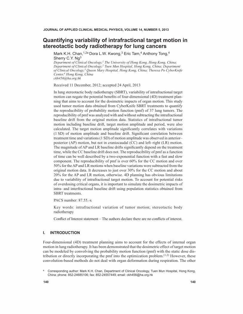
a Corresponding author: Mark K.H. Chan, Department of Clinical Oncology, Tuen Mun Hospital, Hong Kong, China; phone: 852-24685106; fax: 852-24557449; email: [email protected]
Quantifying variability of intrafractional target motion in stereotactic body radiotherapy for lung cancers
Mark K.H. Chan,1,2a Dora L.W. Kwong,3 Eric Tam,4 Anthony Tong,4 Sherry C.Y. Ng3
Department of Clinical Oncology,1 The University of Hong Kong, Hong Kong, China; Department of Clinical Oncology,2 Tuen Mun Hospital, Hong Kong, China; Department of Clinical Oncology,3 Queen Mary Hospital, Hong Kong, China; Theresa Po CyberKnife Center,4 Hong Kong, [email protected]
Received 11 December, 2012; accepted 24 April, 2013
In lung stereotactic body radiotherapy (SBRT), variability of intrafractional target motion can negate the potential benefits of four-dimensional (4D) treatment plan-ning that aims to account for the dosimetric impacts of organ motion. This study used tumor motion data obtained from CyberKnife SBRT treatments to quantify the reproducibility of probability motion function (pmf) of 37 lung tumors. The reproducibility of pmf was analyzed with and without subtracting the intrafractional baseline drift from the original motion data. Statistics of intrafractional tumor motion including baseline drift, target motion amplitude and period, were also calculated. The target motion amplitude significantly correlates with variations (1 SD) of motion amplitude and baseline drift. Significant correlation between treatment time and variations (1 SD) of motion amplitude was observed in anterior–posterior (AP) motion, but not in craniocaudal (CC) and left–right (LR) motion. The magnitude of AP and LR baseline drifts significantly depend on the treatment time, while the CC baseline drift does not. The reproducibility of pmf as a function of time can be well described by a two-exponential function with a fast and slow component. The reproducibility of pmf is over 60% for the CC motion and over 50% for the AP and LR motions when baseline variations were subtracted from the original motion data. It decreases to just over 30% for the CC motion and about 20% for the AP and LR motion, otherwise. 4D planning has obvious limitations due to variability of intrafractional target motion. To account for potential risks of overdosing critical organs, it is important to simulate the dosimetric impacts of intra- and interfractional baseline drift using population statistics obtained from SBRT treatments.
PACS number: 87.55.-x
Key words: intrafractional variation of tumor motion; stereotactic body radiotherapy
Conflict of Interest statement – The authors declare there are no conflicts of interest.
I. IntroductIon
Four-dimensional (4D) treatment planning aims to account for the effects of internal organ motion in lung radiotherapy. It has been demonstrated that the dosimetric effect of target motion can be modeled by convolving the probability motion function (pmf) with the static dose dis-tribution or directly incorporating the pmf into the optimization problem.(1,2) However, these convolution-based methods do not deal with organ deformation during respiration. The other
JournAL oF APPLIEd cLInIcAL MEdIcAL PHYSIcS, VoLuME 14, nuMBEr 5, 2013
140 140

141 chan et al.: Variability of intrafractional target motion in lung SBrt 141
Journal of Applied clinical Medical Physics, Vol. 14, no. 5, 2013
common approach is 4D dose calculation. In this approach, dose distributions are calculated and/or optimized on multiple breathing geometries obtained from a 4D computed tomography (4D CT) dataset, and summed together using deformable image registration. The resulting 4D dose distribution explicitly accounts for the cumulative effect of temporal changes of anatomic structures.(3,4) Such 4D planning technique is particularly useful to incorporate the additional movement of beam aperture in dynamic multileaf (MLC)-based or robotic-based target track-ing radiotherapy.(5,6)
The robustness of any 4D planning regime depends on the reliability of the motion model input. In fact, study using repeated 4D CT has demonstrated that tumor mobility increased between weeks during the treatment course.(7) Experiences from image-guided (IG) radiotherapy also indicated that target exhibited changes of characteristics of the periodic (cyclic) respiration-induced motion and nonperiodic (ultracyclic) baseline motion, in spite of rather stable tumor trajectory between treatment fractions.(8) The random and systematic uncertainties of interfrac-tional target position effectively vary the pmf and, consequently, the dose distribution.
For stereotactic body radiotherapy (SBRT) of lung cancers, intrafractional variation of tumor motion may also be important due to the complex setup procedures and the long beam-on time leading to an increase of overall treatment duration. Purdie et al.(9) acquired cone-beam computed tomography (CBCT) before and after treatment delivery to assess the intrafractional errors of target positions, which included contributions from overall patient movement and target baseline drift. They found a correlation between the target position error and the treat-ment time. Similarly, Sonke et al.(10) used respiratory-correlated CBCT (rCBCT) to quantify the intrafractional target position errors relative to bony anatomy (i.e., intrafractional baseline drift). They found systematic errors (1 SD) of 1.0, 1.4, and 0.6 mm, and random errors of 1.1, 1.5, 0.7 mm in the CC, AP, and LR directions, respectively. Due to the constant treatment time, they did not observe a correlation between the drift of tumor baseline and the treatment time. On the other hand, Suh et al.(11) used continuous tumor motion data extracted from CyberKnife SBRT treatments to obtain statistics of intrafractional tumor motion. They estimated the overall mean cycle-to-cycle variations of tumor motion amplitude and period to be 0.2 cm and 0.8 s, respectively. However, none of these studies (and others) quantified how the variations of tumor motion amplitude and period and baseline affect the reproducibility of pmf.(12) Cai et al.(13) have employed dynamic MRI to study the reproducibility of interfractional lung pmf. However, their motion data was limited to 300 s, which were much shorter than the typical length of actual SBRT treatments (one-half to one hour, and even up to two hours in CyberKnife real-time target tracking SBRT). It is the aim of this study to assess the intrafractional variations of tumor motion and the reproducibility of the pmf on a times scale that corresponds to actual SBRT treatments. It is expected that results obtained in this study shall shed insight into the appropriateness of 4D planning of SBRT for lung cancers.
II. MAtErIALS And MEtHodS
A. Acquisition and analysis of tumor motion dataBetween 2008 and 2011, 37 lesions (15 lower-lobe tumors, 14 middle-lobe tumors, and eight upper-lobe tumors) of a total of 28 patients were treated with SBRT using the CyberKnife robotic radiosurgery system (Accuray Inc., Sunnyvale, CA). There were a total of 128 treat-ment fractions. The target motion data of these patients were obtained from the log files of the Synchrony Respiratory Tracking System (RTS) (Accuray Inc. Sunnyvale, CA). Note that the Synchrony RTS does not track the tumor itself, but records the center-of-mass (COM) of the implanted fiducials as computed by the pair of stereoscopic images. For an elaboration of technical details about the tracking mechanism, see Seppenwoolde et al.(6) and Hoogeman et al.(14) The motion log file contained motion data in three principal directions in the format of t:x,y,z, where t is the time in seconds, x, y, and z are the target positions in millimeter (mm)

142 chan et al.: Variability of intrafractional target motion in lung SBrt 142
Journal of Applied clinical Medical Physics, Vol. 14, no. 5, 2013
in the craniocaudal (CC), left–right (LR), and anterior–posterior (AP) directions. Note that the target motion was based on the estimate of the correlation model that was built using the external breathing signal and the internal fiducials COM’s position. Therefore, it did not strictly represent the true target positions. The mean correlation model errors have been estimated to be better than 0.3 mm.(14)
Prior to the motion analysis, motion traces in each direction were plotted and visually inspected to remove the portions with significant artifacts. To reduce uncertainties of the results, the criteria of exclusion and inclusion of data points recommended by Suh et al.(11) were fol-lowed. In our analysis, one fraction could generate more than one motion trace of shorter periods because the correlation model was forced to rebuild whenever the actual and estimated position of the center-of-mass of implanted fiducials deviated by 3 mm in a row. Furthermore, since couch movements to reposition the patient were not logged by the target localization system (TLS), there were no direct means to join datasets before and after the couch corrective move-ments, unless manual efforts were taken to note these movements. In the following analysis, these short motion traces were combined by subtracting the difference of the last 30-second average of the motion data before model rebuilt and the first 30-second average of the motion data after model rebuilt from the motion data of the rebuilt model. This data joining procedure was illustrated in Fig. 1. To avoid serious error in the analysis of motion statistics, motion data were combined only if the mean amplitude of the rebuilt motion model was within the mean amplitude ± 2 SD of the beginning motion model. Such criteria was rather arbitrary, but was adopted to exclude obvious error resulting from the motion correlation model while not to overly exclude motion data that might represent the actual change of motion characteristics. Because the motion traces before and after model rebuild may exhibit different amplitudes, errors could occur at the connecting points between the fragmented motion data. However, the resulting errors in the determination of cycle-to-cycle period and amplitude were expected
FIG. 1. (A) Two motion traces of the same treatment fraction were showed. They were joined by
subtracting the difference of the last 30-second average of the motion data before model rebuilt (green
solid line) and the first 30-second average of the motion data after model rebuilt (black solid line) from
the motion data of the rebuilt model. (B) The data joining artifact was indicated. The red solid line
represented the ultracyclic target baseline motion. (C) The complete time series of target motion after
the data joining procedure was demonstrated. With the large number of motion cycles, the artifact of
motion data joining is expected to contribute to negligible errors of the overall estimates of target
motion amplitude and period.
Fig. 1. Two motion traces (a) of the same treatment fraction are showed. They were joined by subtracting the difference of the last 30 s average of the motion data before model rebuilt (green solid line) and the first 30 s average of the motion data after model rebuilt (black solid line) from the motion data of the rebuilt model. The data joining artifact (b) was indicated; the red solid line represents the ultracyclic target baseline motion. The complete time series (c) of target motion after the data joining procedure was demonstrated. With the large number of motion cycles, the artifact of motion data joining is expected to contribute to negligible errors of the overall estimates of target motion amplitude and period.

143 chan et al.: Variability of intrafractional target motion in lung SBrt 143
Journal of Applied clinical Medical Physics, Vol. 14, no. 5, 2013
to be averaged out given the large number of breathing cycles. Furthermore, the data joining procedure assumed negligible tumor baseline drift before and after intervening couch shifts. This assumption could introduce error of 1.9 mm (1 SD) in the baseline estimation, as showed in a recent study of diaphragm motion during CBCT acquisition.(15) In this work, 20 motion traces were reconstructed by combining motion traces belonging to two correlation models, and three motion traces were generated with traces from three correlation models of the same treatment fraction.
For each motion trace, the peak-to-peak amplitude was determined by an in-house written code in MATLAB (The MathWorks, Inc. Natick, MA). The code included a low-pass (Gaussian) filter to reduce high frequency noise embedded in the original data, and used the MATLAB built-in algorithm to locate local maxima. Only motion traces of length > 1000 s were included in this analysis.
B. Intrafractional variability of tumor motion baselineOnce the portions of the artifacts were removed, the intrafractional variability of the ultra-cyclic baseline motion was estimated in a two-step process: 1) the reference baseline was established with the first 100 s (starting from the 10th to 110th second) of the motion trace, and 2) a running mean (RM) for the motion traces with a 20 s moving window was created as an approximation of the baseline.
The reason of using 100 s as an estimate of the reference baseline is that it roughly corre-sponds to the duration needed to build a reliable correlation model with eight evenly distributed points along the breathing cycle (two at either extremes and the other six at the mid-exhale and mid-inhale phases), and that it roughly corresponds to the acquisition time of planning 4D CT and verification CBCT. The second step involved extracting the ultracyclic target motion from the motion trace to approximate the time series of mean target positions. For this study, a 20 s moving window was employed to create a RM of the target position inside the window. The evaluation of the baseline drift was started at 110 s (i.e., the next data point to ) and stopped at 10 s from the end of the trace.
c. Intrafractional reproducibility of probability density motion function (pmf)After the motion data was processed as described above, the pmf was calculated by binning the target displacement, with a constant bin size set to 0.05 mm. The reproducibility of intra-fractional pmf was analyzed separately for the CC, AP, and LR target motions. The reference pmf was generated from the same motion data as the reference baseline. It was then compared to the pmfs that were generated every 100 s following the reference pmf to determine the reproducibility R as a function of time t:
(1)
The reproducibility of pmf as a function of time R(t) was stopped until the remaining data were < 100 s. In addition, the influence of baseline drift on the reproducibility of intrafractional pmf was also evaluated by subtracting the ultracyclic baseline motion from the original motion data. This resulted in the reproducibility of pmf due to the cyclic tumor motion, Rc(t)
(2)
where the subscript c indicates the cyclic component of the tumor motion.

144 chan et al.: Variability of intrafractional target motion in lung SBrt 144
Journal of Applied clinical Medical Physics, Vol. 14, no. 5, 2013
d. Statistical analysisStatistical correlations between variables were analyzed by linear regression, exponential regression, and ANOVA with two and more factors using the Statistical Toolbox of MATLAB. P-value for Pearson’s correlation (r) resulting from the linear regression was computed using a Student’s t-distribution. The Student’s t-test was also used to compare groups and variables. A p-value < 0.05 is considered statistically significant.
III. rESuLtS
A total of 154 motion traces were extracted. The longest and shortest durations were 6000 s and 1200 s (median = 3400 s), respectively. The principal motion coincides with the CC direction. There is an observable trend of increasing CC, AP, and LR motion amplitude in lower lobe tumors than upper and middle lobe tumors (p < 0.05). The overall mean of individual treatment fraction means of target motion amplitude is 6.0 ± 4.6 mm (range: 0.2–18.7 mm), 1.7 ± 1.2 mm (0.2–5.8 mm), and 0.9 ± 0.8 mm (0.0–3.7mm) in the CC, AP, and LR directions, respectively. The overall target motion period is 3.6 ± 0.6 s, with individual treatment fraction means ranging from (2.0–5.6 s). Lengths of the exhale and the inhale period of the patient population range from 0.9–2.2 s (mean : 1.5 s) and 1.1–3.4 s (mean : 2.0 s), respectively.
In Fig. 2, the linear regressions show increasing variability of intrafractional target motion amplitude (1 SD) with the motion amplitude in all directions (CC: r = 0.80, p < 10-30; AP: r = 0.76, p < 10-24; and LR: r = 0.76, p < 10-24). From Fig. 3, it was observed that the correlations of the motion amplitude variability and treatment time are moderate for the AP motion and weak for the CC and LR motions. ANOVA indicates that for the CC and LR directions, the variability of motion amplitude significantly depends on the tumor location (p < 0.05) but not on the treatment time (p = 0.98 for CC, and p = 0.073 for LR), whereas for the AP direction the variability depends on both tumor site (p = 0.004) and treatment time (p = 0.002). Variations (1 SD) of the exhale and inhale lengths versus the breathing cycle periods are plotted in Fig. 4.
FIG. 2. Linear regressions of the motion amplitude and the motion variability (1 SD) in the
cranio-caudal (A), anterior-posterior (B), and left-right (C) directions. Each circle represents each of
the 128 motion traces. The linear fits and Pearson’s correlation coefficients of the data are also given.
(D) Box-and-Whisker plot of the coefficient of variation (CV) of each motion component is shown.
Outliers with a value that is more than 1.5 times the interquartile range away from the top or bottom of
the box are marked with a red + sign.
Fig. 2. Linear regressions of the motion amplitude and the motion variability (1 SD) in the craniocaudal (a), anterior–posterior (b), and left–right (c) directions. Each circle represents each of the 128 motion traces. The linear fits and Pearson’s correlation coefficients of the data are also given. Box-and-whisker plot (d) of the coefficient of variation (CV) of each motion component is shown. Outliers with a value that is more than 1.5 times the interquartile range away from the top or bottom of the box are marked with a red + sign.

145 chan et al.: Variability of intrafractional target motion in lung SBrt 145
Journal of Applied clinical Medical Physics, Vol. 14, no. 5, 2013
A slightly higher correlation is observed between the breathing cycle period and the exhale length (r = 0.94) than between the breathing cycle period and the inhale length (r = 0.87). Statistically, difference of motion period between lower lobe tumors and upper and middle tumors is insignificant (3.5 s vs. 3.7 s; p = 0.08). However, the F-test shows greater variance of the length of exhale state than inhale state (p < 10-6) of individual treatment fractions.
Figure 5 shows distribution of the baseline drift in each direction and the distribution of the 3D baseline drift. The population statistics in terms of group mean, systematic, and random
FIG. 3. Relationship between variability of motion amplitude (1 SD) and time for each motion axis.
Each circle represents each of the 128 motion traces. The red lines are the best fits in the least-square
sense. The Pearson’s correlation coefficients r are shown.
FIG. 4. Variation (1 SD) of cycle period was plotted against the variations (1 SD) of the length of
exhale (blue dot) and inhale (red dot) states. Each circle represents each of the 128 motion traces. The
linear fits and Pearson’s correlation coefficients are also given.
Fig. 3. Relationship between variability of motion amplitude (1 SD) and time for each motion axis. Each circle represents each of the 128 motion traces. The red lines are the best fits in the least-square sense. The Pearson’s correlation coef-ficients r are shown.
Fig. 4. Variation (1 SD) of cycle period was plotted against the variations (1 SD) of the length of exhale (blue dot) and inhale (red dot) states. Each circle represents each of the 128 motion traces. The linear fits and Pearson’s correlation coefficients are also given.
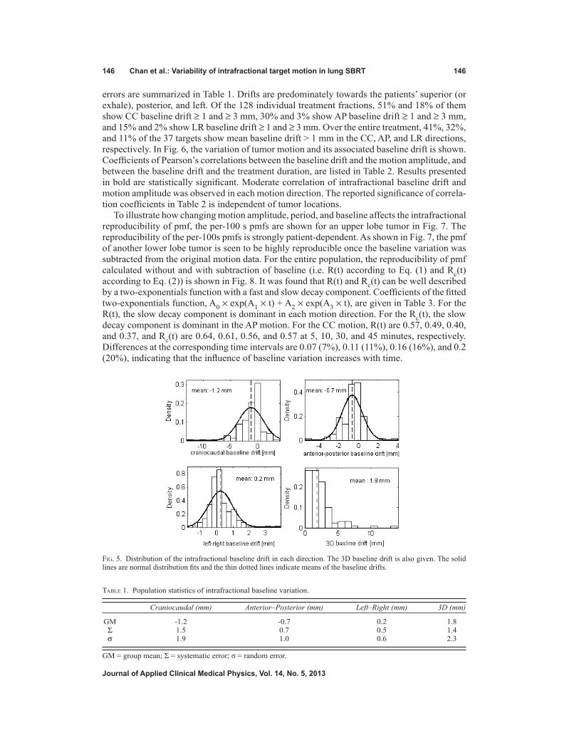
146 chan et al.: Variability of intrafractional target motion in lung SBrt 146
Journal of Applied clinical Medical Physics, Vol. 14, no. 5, 2013
errors are summarized in Table 1. Drifts are predominately towards the patients’ superior (or exhale), posterior, and left. Of the 128 individual treatment fractions, 51% and 18% of them show CC baseline drift ≥ 1 and ≥ 3 mm, 30% and 3% show AP baseline drift ≥ 1 and ≥ 3 mm, and 15% and 2% show LR baseline drift ≥ 1 and ≥ 3 mm. Over the entire treatment, 41%, 32%, and 11% of the 37 targets show mean baseline drift > 1 mm in the CC, AP, and LR directions, respectively. In Fig. 6, the variation of tumor motion and its associated baseline drift is shown. Coefficients of Pearson’s correlations between the baseline drift and the motion amplitude, and between the baseline drift and the treatment duration, are listed in Table 2. Results presented in bold are statistically significant. Moderate correlation of intrafractional baseline drift and motion amplitude was observed in each motion direction. The reported significance of correla-tion coefficients in Table 2 is independent of tumor locations.
To illustrate how changing motion amplitude, period, and baseline affects the intrafractional reproducibility of pmf, the per-100 s pmfs are shown for an upper lobe tumor in Fig. 7. The reproducibility of the per-100s pmfs is strongly patient-dependent. As shown in Fig. 7, the pmf of another lower lobe tumor is seen to be highly reproducible once the baseline variation was subtracted from the original motion data. For the entire population, the reproducibility of pmf calculated without and with subtraction of baseline (i.e. R(t) according to Eq. (1) and Rc(t) according to Eq. (2)) is shown in Fig. 8. It was found that R(t) and Rc(t) can be well described by a two-exponentials function with a fast and slow decay component. Coefficients of the fitted two-exponentials function, A0 × exp(A1 × t) + A2 × exp(A3 × t), are given in Table 3. For the R(t), the slow decay component is dominant in each motion direction. For the Rc(t), the slow decay component is dominant in the AP motion. For the CC motion, R(t) are 0.57, 0.49, 0.40, and 0.37, and Rc(t) are 0.64, 0.61, 0.56, and 0.57 at 5, 10, 30, and 45 minutes, respectively. Differences at the corresponding time intervals are 0.07 (7%), 0.11 (11%), 0.16 (16%), and 0.2 (20%), indicating that the influence of baseline variation increases with time.
FIG. 5. Distribution of the intrafractional baseline drift in each direction. The 3D baseline drift is
also given. The solid lines are normal distribution fits and the thin dotted lines indicate means of the
baseline drifts.
Fig. 5. Distribution of the intrafractional baseline drift in each direction. The 3D baseline drift is also given. The solid lines are normal distribution fits and the thin dotted lines indicate means of the baseline drifts.
Table 1. Population statistics of intrafractional baseline variation.
Craniocaudal (mm) Anterior–Posterior (mm) Left–Right (mm) 3D (mm)
GM -1.2 -0.7 0.2 1.8 Σ 1.5 0.7 0.5 1.4 σ 1.9 1.0 0.6 2.3
GM = group mean; Σ = systematic error; σ = random error.

147 chan et al.: Variability of intrafractional target motion in lung SBrt 147
Journal of Applied clinical Medical Physics, Vol. 14, no. 5, 2013
FIG. 6. Illustration of the variation of tumor motion in the each direction for one selected patient.
The blue solid lines are the original motion data, green lines show the baselines and the red dotted lines
are the original motion data subtracting the baseline (i.e. cyclic motion). The CC baseline drift reaches
a minimum of -4.0 mm halfway through the treatment and return to -0.2 mm at the end of the
treatment.
Fig. 6. Illustration of the variation of tumor motion in the each direction for one selected patient. The blue solid lines are the original motion data, green lines show the baselines, and the red dotted lines are the original motion data subtracting the baseline (i.e., cyclic motion). The CC baseline drift reaches a minimum of -4.0 mm halfway through the treatment and returns to -0.2 mm at the end of the treatment.
Table 2. Correlations of the magnitude of intrafractional baseline drift with the amplitude of intrafractional target motion and treatment time.
Baseline Craniocaudal Anterior–Posterior Left–Right
motion amplitude 0.42 0.37 0.36 time 0.08 0.26 0.16
Values are the Pearson’s correlation coefficients r, and values presented in bold are statistically significant.

148 chan et al.: Variability of intrafractional target motion in lung SBrt 148
Journal of Applied clinical Medical Physics, Vol. 14, no. 5, 2013
Fig. 7. Calculated probability motion functions (pmf) of intrafractional target motion without subtraction of target baseline motion (i.e., ultracyclic plus cyclic target motion (a)-(f)), and with subtraction of the target baseline motion (i.e., cyclic target motion (g)–(l)), for a lower- and upper-lobe tumor. Each red solid line represents the per-100 s pmf, and the black solid line is the reference pmf calculated using the first 100 s motion data. The blue dotted line is the averaged pmf of the entire treatment. The upper-lobe tumor is not only associated with noticeable baseline variation, but also associated with significant variability of target motion amplitude and period. The lower-lobe tumor, on the other hand, is associated with excellent reproducibility of the pmf in spite of the baseline variations.

149 chan et al.: Variability of intrafractional target motion in lung SBrt 149
Journal of Applied clinical Medical Physics, Vol. 14, no. 5, 2013
IV. dIScuSSIon
This study analyzed tumor motion data obtained from the log files in CyberKnife real-time target tracking SBRT. Previous studies that employ 4D simulation/cone-beam CT provided estimate of tumor location errors and evaluation of motion trajectory at certain time points (e.g., before and after the treatment).(16-18) Continuous fluoroscopic imaging has the potential to track the tumor motion trajectory throughout the treatment, but it raises concerns of additional exposure to the patient, which requires substantial justification.(8,19) This study inferred the tumor location from the fiducial markers implanted in or near the tumor, and derived the motion of the tumor from continuously updated correlation model based on the external breathing signal and the internal marker position. It is known that correlation between the internal markers and the tumor is not perfect(20) and correlation error between the external breathing signal and the internal markers exists,(14) but the correlation motion data still offers valuable information about the continuous motion of tumor within a time frame relevant to CyberKnife SBRT and beam-gated SBRT.
For our patient population, the overall cycle-to-cycle motion amplitude in the principal motion axis (craniocaudal) is 6.0 ± 4.6 mm (SD), which is close to means of 5.0 ± 1.6 mm and 9.9 ± 6.4 mm reported by Suh et al.(11) and Guckenberger et al.,(16) respectively. Similarly, the overall cycle-to-cycle period is 3.6 ± 0.6 s (SD), which is very similar to the mean of three
FIG. 8. Calculated reproducibility of per-100 s probability motion functions starting at the 110th
second up to the 3400th
second (median treatment length of the patient group). The red triangle
corresponds to the motion data with subtraction of the ultracyclic baseline (i.e. cyclic motion) and the
blue square is the original motion data without subtraction of the baseline (i.e. the cyclic plus
ultracyclic motion), respectively. The black and green lines are the two-exponential fits to the data
using the Levenberg-Marquardt algorithm. R2 of the fits are also given.
Fig. 8. Calculated reproducibility of per-100 s probability motion functions starting at the 110th second up to the 3400th second (median treatment length of the patient group). The red triangle corresponds to the motion data with subtraction of the ultracyclic baseline (i.e., cyclic motion) and the blue square is the original motion data without subtraction of the baseline (i.e., the cyclic plus ultracyclic motion), respectively. The black and green lines are the two-exponential fits to the data using the Levenberg-Marquardt algorithm. R2 of the fits are also given.
Table 3. Coefficients of the two-exponential fits to the reproducibility of probability motion function (pmf) calculated for the motion data including baseline R(t) and excluding baseline Rc(t).
A0 A1 A2 A3 R2
R(t) CC 1.7E-01 -2.4E-03 4.9E-01 -1.0E-4 (1.4E-01, 2.1E-01) (-3.5E-03, -1.2E-03) (4.6E-01, 5.3E-01) (-1.4E-04,-8.4E-05) 0.98
AP 3.9E-01 -1.5E-03 2.8E-01 -9.23E-05 (3.3E-01, 4.6E-01) (-1.9E-03, -1.0E-03) (2.0E-01, 3.5E-01) (-1.8E-05,-4.5E-06) 0.99
LR 2.7E-01 -2.9E-03 4.1E-01 -2.8E-04 (2.3E-01, 3.2E-01) (-3.9E-03, -1.9E-03) (3.7E-01, 4.5E-01) (-3.2E-04,-2.4E-04) 0.99
Rc(t) CC 1.2E-01 -2.2E-03 5.9E-01 -1.9E-05 (8.9E-2, 1.4E-01) (-3.5E-03, -1.0E-03) (5.7E-01, 6.1E-03) (-3.3E-05,-4.2E-06) 0.92
AP 2.5E-01 -9.92E-04 4.6E-01 -1.6E-06 (1.5E-01, 3.4E-01) ( 1.5E-03, -4.7E-04) (3.6E-01, 5.7E-01) (-6.0E-05,-5.7E-05) 0.98
LR 1.7E-01 -3.7E-03 5.6E-01 -5.9E-05 (1.3E-01, 2.2E-01) (-5.3E-03, -2.0E-03) (5.4E-01, 5.8E-01) (-7.3E-05,-4.6E-05) 0.96
Values given in brackets are the 95% confidence intervals of the fit coefficients.CC = craniocaudal motion; AP = anterior–posterior motion; LR = left–right motion.

150 chan et al.: Variability of intrafractional target motion in lung SBrt 150
Journal of Applied clinical Medical Physics, Vol. 14, no. 5, 2013
other patient populations (3.7 s).(8,11,20) Unlike the CC motion that shows greater amplitude in lower lobe tumors than in upper and middle lobe tumors, the motion period shows no noticeable dependence of the tumor location. In this work, we found that the exhale length is more variable than the inhale length. This implies that the dose-weighting scheme of 4D dose accumulation shall have greater uncertainty contributing from the exhale phases.
Previously, Bissonnette et al.(12) found that the inter- and intra-acquisition variability of tumor mobility increased with the averaged motion amplitude. The study also found that the motion amplitude is not only a significant predictor of the intrafractional variability (1 SD) of tumor motion, but also a significant predictor of the magnitude of intrafractional baseline variation in each direction. This suggests that larger PTV margin may be needed for lower lobe tumor in nontarget-tracking SBRT treatments. Several studies have showed that active breath control and abdominal compression are effective to limit motion amplitude, but these techniques also resulted in greater variability of target position and motion amplitude,(12,21) and are unnecessary and impractical in target-tracking SBRT concerning the long treatment time. Therefore, the need of larger margin for lower lobe tumors in conventional SBRT treatments remains, since motion reducing techniques are frequently applied to these tumors with the greatest mobility.
From the results of Fig. 3 and Table 2, neither the variability of cyclic (CC, LR, and 3D) target motion nor the ultracyclic (CC and 3D) baseline drift appears to increase or decrease with treatment time for the scale from 1200 s to 6000 s. As previously demonstrated by Guckenburger et al.(16) using four repeated 4D CT scans at ten-minute intervals, the intrafractional tumor motion was relatively stable, although significant variations were possible in patients with poor pulmonary function. Bisonnette and colleagues similarly reported that the tumor motion varia-tion was limited to < 1 mm and did not differ by the treatment fraction time. For a series of 129 patients from the United States using 3D CBCT, Shah et al.(17) showed that the intrafractional (3D) baseline drift > 5 mm was significantly more frequent when treatment time was longer (22.6 ± 5.9 min vs. 20.7 ± 4.9 min), and the (3D) baseline drift > 2 mm was found to correlate with longer treatment times. As demonstrated in Fig. 6, the baseline could deviate from its starting position in the middle of the treatment and return to nearly the starting position at the end of the treatment. Therefore, taking samples of the tumor baseline position at the start and at the end of the treatment is likely to exclude significant change in the middle of the treatment, leading to underestimation of the intrafractional baseline drift. For the CC motion, the mean baseline drift estimated using the entire time series and estimated using the first 100 s and the last 100 s (a scenario corresponds to using CBCT) differs by 0.8 mm. Despite the notable dif-ferences between this study using motion data from the entire treatment and others using 4D CT or CBCT to derive the baseline position, the calculated statistics of the intrafractional baseline drift is remarkably similar.(10,16,18) The results of Sonke et al.(10) and ours similarly indicated posterior and superior baseline drifts, whereas Guckenberger et al.(16) indicated posterior and inferior drifts. It is unknown whether the directions are associated with the gravity and other physio- and psychological processes, such as gradual relaxation of muscle and stress.
Constant motion pattern is the fundamental assumption for most 4D treatment planning strategy. Figure 7 clearly shows that this assumption hardly holds. The reproducibility of pmf is affected by not only the cyclic target motion but also the ultracyclic target baseline drift (Fig. 8). The influence of baseline variation is more important in the first 15 minutes and then gradually diminishes. It is also more important in the AP direction. We found that the reproducibility of population pmf decays following a two-exponentials function that has a fast and slow decay component. The underlying mechanisms of the fast and slow decay are not fully understood. One possible explanation for the fast decay component is the psychological nervousness of the patient during the beginning of treatment. For the AP motion, the weight of the fast decay component is larger that of the slow decay component in the R(t) curve and becomes smaller in the Rc(t) curve. This signifies that the fast decay component is strongly related to the ultracyclic baseline drift. The observed motion reproducibility curve shown in Fig. 8 seems to support our clinical practice of allowing patients to rest on the CT scanner couch for about ten minutes

151 chan et al.: Variability of intrafractional target motion in lung SBrt 151
Journal of Applied clinical Medical Physics, Vol. 14, no. 5, 2013
before the 4D CT simulation. Overall, the cyclic target motion is relatively stable over time, with reproducibility over 50% for the AP and LR motions, and 60% for the CC motion up to 50 minutes.
The general approach of 4D planning is to accumulate dose using a patient breathing model. The ultimate question is whether the respiratory phases correspond to the exact spatial location over the fraction as it had been in the simulation 4D CT images. Attempts have been made to incorporate such variability of the pmf into 4D planning, but that requires estimation and generation of error bars associated with the pmf.(2) As demonstrated by Fig. 7, the shape of the pmf can be far more “random” than those used to test the robustness of different probabilistic optimization algorithms.(2,22) It has been demonstrated that target tracking techniques such as dynamic MLC tracking, robotic respiratory tracking, and tumor trailing strategy based on the moving average algorithm have the ability to adapt the baseline variation, but such adaptation is hardly reflected in the 4D dose calculation. Recently, Chan et al.(23) have demonstrated that the sensitivity of 4D dose calculation to the variation of target motion differed by organs of interest in target-tracking SBRT, with the greatest dosimetric errors observed in structures that were static or moved asynchronously with respect to the tracking object. Since planning risk volumes (PRV) have the limitations in serially functioning organs such as the spinal cord,(24) we suggest to simulate the intrafractional (and also interfractional) baseline drifts using the population data during treatment planning to avoid potential risks of overdosing these critical organs.
V. concLuSIonS
This study shows that intrafractional target motion, excluding the influence of baseline drift, is relatively stable with reproducibility over 60% in CC and 50% in AP and LR directions within a time frame that is typical of lung SBRT. However, tumor baseline can change substantially in SBRT and effectively reduces the reproducibility of pmf in the majority of patients. These results suggest that methods based on dose convolution technique or explicit 4D dose calcula-tion may only serve as a first-order approximation to the dosimetric effects of target motion. It may be important to simulate the interfractional in addition to intrafractional baseline drifts to avoid potential risks of normal tissue complications, particularly if tumor is close to the organs at risk.
AcknowLEdgMEntS
This work was partially supported by the Hong Kong Adventist Hospital.
rEFErEncES
1. Lujan AE, Balter JM, Ten Haken RK. A method for incorporating organ motion due to breathing into 3D dose calculations in the liver: Sensitivity to variations in motion. Med Phys. 2003;30(10):2643–49.
2. Geneser S, Kirby RM, Wang B, Salter B, Joshi S. Incorporating patient breathing variability into a stochastic model of dose deposition for stereotactic body radiation therapy. Int Process Med Imaging. 2009;21:688–700.
3. Keall PJ, Joshi S, Vedam SS, Siebers JV, Kini VR, Moohan R. Four-dimensional radiotherapy planning for DMLC-based respiratory motion tracking. Med Phys. 2005;32(4):942–51.
4. Starkschall G, Britton K, McAleer MF, et al. Potential dosimetric benefits of four-dimensional radiation treatment planning. Int J Radiat Oncol Biol Phys. 2009;73(5):1560–65.
5. Sawant A, Venkat R, Srivastava V, et al. Management of three-dimensional intrafraction motion through real-time DMLC tracking. Med Phys. 2008;35(5):2050–61.
6. Seppenwoolde Y, Berbeco RI, Nishioka S, Shirato H, Heijmen B. Accuracy of tumor motion compensation algorithm from a robotic respiratory tracking system: a simulation study. Med Phys. 2007;34(7):2774–84.

152 chan et al.: Variability of intrafractional target motion in lung SBrt 152
Journal of Applied clinical Medical Physics, Vol. 14, no. 5, 2013
7. Britton KR, Starkschall G, Tucker SL, et al. Assessment of gross tumor volume regression and motion changes during radiotherapy for non–small-cell lung cancer as measured by four-dimensional computed tomography. Int J Radiat Oncol Biol Phys. 2007;68(4):1036–46.
8. Seppenwoolde Y, Shirato H, Kitamura K, et al. Precise and real-time measurement of 3D tumor motion in lung due to breathing and heartbeat, measured during radiotherapy. Int J Radiat Oncol Biol Phys. 2002;53(4):822–34.
9. Purdie TG, Bissonnette JP, Franks K, et al. Cone-beam computed tomography for on-line image guidance of lung stereotatic radiotherapy: localization, verification, and intrafrational tumor position. Int J Radiat Oncol Biol Phys. 2007;68(1):243–52.
10. Sonke J-J, Rossi M, Wolthaus J, van Herk M, Damen E, Belderbos J. Frameless stereotactic body radio-therapy for lung cancer using four-dimensional cone beam CT guidance. Int J Radiat Oncol Biol Phys. 2009;74(2):567–74.
11. Suh Y, Dieterich S, Cho B, Keall PJ. An analysis of thoracic and abdominal tumour motion for stereotactic body radiotherapy patients. Phys Med Biol. 2008;53(13):3623–40.
12. Bissonnette J-P, Franks KN, Purdie TG, et al. Quantifying interfraction and intrafraction tumor motion in lung stereotactic body radiotherapy using respiration-correlated cone beam computed tomography. Int J Radiat Oncol Biol Phys. 2009;75(3):688–95.
13. Cai J, Read PW, Larner JM, Jones DR, Benedict SH, Sheng K. Reproducibility of interfraction lung motion probability distribution function using dynamic MRI: statistical analysis. Int J Radiat Oncol Biol Phys. 2008;72(4):1228–35.
14. Hoogeman M, Prévost J-B, Nuyttens J, Poll J, Levendag P, Heijmen B. Clinical accuracy of the respiratory tumor tracking system of the Cyberknife: assessment by analysis of log files. Int J Radiat Oncol Biol Phys. 2009;74(1):297-303.
15. Rit S, van Herk M, Zijp L, Sonke JJ. Quantification of the variability of diaphragm motion and implications for treatment margin construction. Int J Radiat Oncol Biol Phys. 2012;82(3):e399–e407.
16. Guckenberger M, Meyer J, Wilbert J, et al. Intra-fractional uncertainties in cone-beam CT based image-guided radiotherapy (IGRT) of pulmonary tumors. Radiother Oncol. 2007;83(1):57–64.
17. Shah C, Grills IS, Kestin LL, et al. Intrafraction variation of mean tumor position during image-guided hypof-ractionated stereotactic body radiotherapy for lung cancer. Int J Radiat Oncol Biol Phys. 2012;82(5):1636–41.
18. Worm ES, Hansen AT, Petersen JB, Muren LP, Praestegaard LH, Heyer M. Inter- and intrafractional localisa-tion errors in cone-beam CT guided stereotactic radiation therapy of tumours in the liver and lung. Acta Oncol. 2010;49(7):1177–83.
19. Berbeco RI, Mostafavi H, Sharp GC, Jiang SB. Towards fluoroscopic respiratory gating for lung tumours without radiopaque markers. Phys Med Biol. 2005;50(19):4481–90.
20. Seppenwoolde Y, Wunderink W, Wunderink-van Veen SR, Storchi P, Mendez Romero A, Heijmen BJ. Treatment precision of image-guided liver SBRT using implanted fiducial markers depends on marker–tumour distance. Phys Med Biol. 2011;56(17):5445–68.
21. Nielsen TB, Hansen VN, Westberg J, Hansen O, Brink C. A dual centre study of setup accuracy for thoracic patients based on cone-beam CT data. Radiother Oncol. 2012;102(2):281–86.
22. Heath E, Unkelbach J, Oelfke U. Incorporating uncertainties in respiratory motion into 4D treatment plan opti-mization. Med Phys. 2009;36(7):3059–71.
23. Chan MK, Kwong DL, Ng SC, Tong AS, Tam EK. Accuracy and sensitivity of four-dimensional dose calculation to systematic motion variability in stereotatic body radiotherapy (SBRT) for lung cancer. J Appl Clin Med Phys. 2012;13(6):303–17.
24. Stroom JC and Heijmen BJM. Limitations of the planning organ at risk volume (PRV) concept. Int J Radiat Oncol Biol Phys. 2006;66(1):279–86.

a Corresponding author: Congying Xie, Radiotherapy and Chemotherapy Department of the 1st Affiliated Hospital of Wenzhou Medical College, No.2 Fuxue Lane, Wenzhou, China 325000; phone: 0086-577-88069316; fax: 0086-577-88069370; email: [email protected]
CRT combined with a sequential VMAT boost in the treatment of upper thoracic esophageal cancer
Xiance Jin, Jinling Yi, Yongqiang Zhou, Huawei Yan, Ce Han, Congying Xiea
Department of Radiotherapy and Chemotherapy, the 1st Affiliated Hospital of Wenzhou Medical University, Wenzhou, [email protected]
Received 16 December, 2012; accepted 27 May, 2013
The purpose of this study is to investigate the potential benefits of conformal radiotherapy (CRT) combined with a sequential volumetric-modulated arc therapy (VMAT) boost in the treatment of upper thoracic esophageal cancer. Ten patients with upper thoracic esophageal cancer previously treated with CRT plus a sequen-tial VMAT boost plan were replanned with CRT plus an off-cord CRT boost plan and a full course of VMAT plan. Dosimetric parameters were compared. Results indicated that CRT plus off-cord CRT boost was inferior in planning target volume (PTV) coverage, as indicated by the volume covered by 93% (p = 0.05) and 95% (p = 0.02) of the prescription dose. The full course VMAT plan was superior in conformal index (CI) and conformation number (CN), and produced the highest protection for the spinal cord. CRT plus a VMAT boost demonstrated significant advantages in decreasing the volume of the lung irradiated by a dose of 10 Gy (V10, p = 0.007), 13 Gy (V13, p = 0.003), and 20 Gy (V20, p = 0.001). The full course VMAT plan demonstrated the lowest volume of lung receiving a dose of 30 Gy. CRT plus a VMAT boost for upper thoracic esophageal cancer can improve the target coverage and reduce the volume of lung irradiated by an intermediate dose. This combination may be a promising treatment technique for patients with upper thoracic esophageal cancer.
PACS number: 87.53.Kn, 87.55.x, 87.55.D, 87.55.dk
Key words: volumetric-modulated arc therapy, conformal radiotherapy, boost phase, upper thoracic esophageal cancer
I. InTRoduCTIon
Conformal radiotherapy (CRT) is still the treatment of choice for esophageal cancer, with parallel opposed, antero-posterior and postero-anterior (APPA) fields for the first phase and a second phase with off-cord lateral or oblique parallel opposed beams.(1) In order to constrain the dose to spinal cord strictly within its tolerant limit, conformal plans may unavoidably compromise target coverage due to its unfavorable geometry close to spinal cord. As such, intensity-modulated radiation therapy (IMRT) has been reported to provide superior target coverage while reducing doses to organs at risk (OAR) of cervical esophageal cancer.(2) A full course of IMRT usually has not been recommended for thoracic cancer because of the widely distributed low dose levels surrounding the planning target volume (PTV).(3,4) A hybrid tech-nique that combines conformal fields with IMRT fields on a daily fraction basis for lung and esophageal cancer patients has been suggested to reduce the volume of the lung irradiated by relatively low dose levels.(5)
JouRnAL oF APPLIEd CLInICAL MEdICAL PHYSICS, VoLuME 14, nuMBER 5, 2013
153 153

154 Jin et al.: CRT plus VMAT for esophageal cancer 154
Journal of Applied Clinical Medical Physics, Vol. 14, no. 5, 2013
With the continued development in radiotherapy delivery techniques, volumetric-modulated arc therapy (VMAT) has begun to replace conventional IMRT in the treatment of several cancers. Several studies have demonstrated that VMAT is able to produce dosimetric plans equivalent to those of IMRT.(6-8) At the same time, VMAT is also able to reduce the number of monitor units and the required delivery time in comparison to IMRT.(6-8) Comparative studies on VMAT and IMRT in the treatment of esophageal cancer also indicate that VMAT is able to achieve comparable target coverage and OAR sparing with reduced monitor units and delivery time.(9,10) However, a full course VMAT plan for the treatment of esophageal cancer patients would exhibit the same problem as a full course IMRT plan. The purpose of this study is to investigate the potential benefit of applying the VMAT technique in the second boost phase instead of using off-cord conformal beams in the treatment of upper thoracic esophageal cancer patients following the first APPA phase.
II. MATERIALS And METHodS
A. PatientsTen patients with upper thoracic esophageal cancer, who were previously treated in our depart-ment with APPA CRT beams for the first phase and followed with a single-arc VMAT boost, were enrolled in this study. Each patient was replanned retrospectively via the Pinnacle treat-ment planning system (Philips, clinical version 9.2; Fitchburg, WI). Patient staging information according to the AJCC staging system (AJCC, 2002) and other relevant characteristics are summarized in Table 1.
Gross tumor volume (GTV), clinical target volume (CTV), PTV, and nodes were contoured by a physician according to the RTOG 0436 protocol.(11) The GTV included the gross tumor and involved nodes as defined by diagnostic CT, oesophagogastroscopy, endoscopic ultrasound, and PET scan. The CTV was delineated with 3–5 cm superior–inferior margins and 1 cm lat-eral and anterior–posterior margins with respect to the GTV. The PTV was delineated with a 0.5 cm margin from the CTV. For the sake of data consistence, the PTVs of this enrolled cohort patients were the same for both the initial and boost plans. The spinal cord, lung, and heart were contoured as OARs on each image.
B. Planning schemesThree planning schemes were generated for each patient. Scheme 1 is CRT initial plus off-cord CRT boost, scheme 2 is CRT initial plus a sequential VMAT boost, and scheme 3 is a full course of VMAT plan — that is, one VMAT plan for the whole treatment course. The prescription dose of CRT initial plan was 2 Gy × 18 fractions for a total dose of 36 Gy with APPA beams, followed by 2 Gy × 12 fractions for a total dose of 24 Gy with off-cord conformal beams. The
Table 1. Patient staging and characteristics.
Patient Staging GTV (cm3) CTV (cm3) PTV (cm3)
1 T3N1M1 25.3 195.3 303.0 2 T3N0M1 15.7 85.7 146.4 3 T3N1M1 15.4 155.5 230.3 4 T2N1M0 17.3 175.3 219.6 5 T3N1M1 19.4 97.4 167.0 6 T2N0M0 16.0 96.0 149.0 7 T4N1M1 35.8 358.8 477.9 8 T2N1M1 12.1 109.1 203.2 9 T4N1M1 34.3 342.3 513.2 10 T3N1M1 37.8 257.8 363.7

155 Jin et al.: CRT plus VMAT for esophageal cancer 155
Journal of Applied Clinical Medical Physics, Vol. 14, no. 5, 2013
prescription dose of CRT plus a sequential boost VMAT was 2 Gy × 18 fractions for a total dose of 36 Gy with initial CRT APPA beams, followed by a single-arc VMAT boost plan with a prescription of 2 Gy × 12 fractions. The prescription dose for the full course VMAT plan was 60 Gy over 30 fractions (2 Gy × 30 fractions). For VMAT plan optimization, constraint leaf motion of 0.46 cm/deg and final arc space degree of 4 were employed. A start angle of 181° and a stop angle of 180° were applied for one-arc plans using clockwise (CW) rotation direction. The maximum constraint dose for the spinal cord was 400 cGy for the sequential VMAT boost plan, and 4500 cGy for the full course VMAT plan. The optimization objectives were set for the PTV, spinal cord, and lung for the VMAT plans. For upper thoracic esophageal cancer, only a very small part of heart was involved in the treatment field; the constraint on heart had little effect on the plan quality, so we did not include the heart in the inverse optimization.
All plans were optimized to reach clinically acceptable levels. For instance, the maximum dose for the spinal cord was less than 45 Gy, whereas the volume of the lung irradiated by a dose of 20 Gy (V20) and 30 Gy (V30) was less than 30% and 20%, respectively. For PTV coverage, 95% of PTV should be covered by 95% of the prescription dose, unless the spinal cord limit was violated.
C. Plan evaluation and comparisonThe following plan quality indices were calculated from the dose-volume histogram (DVH) data for evaluation and comparison.
Target coverage (TC) of PTV was calculated to describe the percent volume of PTV covered by the prescription dose:
(1)
TCVT,Pi
VT
=
where VT,Pi is the target volume that was covered by the prescription isodose, which was set at 95% in this study. VT is the volume of the target.
A homogeneity index similar to that defined in the ICRU 62 Report was adapted for PTV to study the dose distribution homogeneity across the PTV:(12)
(2)
HI V95 – V110V95
=
The conformity index (CI)(13) and conformation number (CN)(14) were also calculated for PTV:
(3)
CIVT,Pi
VPi
=
(4)
CNVT,Pi
VT
VT,Pi
VPi
= ×
where VPi is the volume that was covered by the prescription isodose. The maximum value of CI is 1, corresponding to a perfect coverage of PTV. CN is the complementary information designed to compensate for defects in the TC and CI. The first term of Eq. (4) stands for the coverage of the target volume. The second term refers to the volume of healthy tissue receiving a dose equal to or greater than the prescribed dose. CN can take values between 0 and 1.

156 Jin et al.: CRT plus VMAT for esophageal cancer 156
Journal of Applied Clinical Medical Physics, Vol. 14, no. 5, 2013
Radiobiological ranking indices, TCP and NTCP, were also calculated using the Niemierko and Goiten model.(15) Based on the equivalent uniform dose (EUD), the tumor control prob-ability (TCP) can be calculated by:
(5)
TCPTCD50
EUD
=4
1
1
[ ] γ50+
where TCD50 is the tumor dose required to produce 50% of TCP, and γ50 is the slope of the dose response at 50% of TCP. These tumor-specific parameters were cited from a study by Okunieff et al.(16) The EUD is defined as the absorbed dose that, if homogeneously delivered to a tumor, would cause the same expected number of clonogens to survive as the actual nonhomogeneous absorbed dose distribution would. Clonogen survival is a stochastic magnitude governed by Poisson statistics, while EUD is obtained as an expected value:
EUD viDa=
1a( )ΣN
1 i (6)
where N is the number of voxels in the structure of interest, Di is the dose in the ith voxel vi, and a is the tumor’s normal tissue-specific parameters that describe the dose-volume effect. TCP of PTV was calculated for the purpose of plan evaluation.
In the case of normal tissue, the normal tissue complication probability (NTCP) is deter-mined as:
(7)
NTCPTD50
EUD
=4
1
1
[ ] γ50+
where TD50 is the dose at which the probability of complication becomes 50% in five years, and γ50 is the slope of the sigmoidal dose response curve of normal tissue at 50% complica-tion probability. These tissue-specific parameters were based on the Niemierko and Goiten model.(15) NTCP of the spinal cord, heart, and lungs were calculated for plan evaluation.
The mean dose (Dmean) and maximum dose (Dmax) for OARs were calculated and compared. The volume of hearts irradiated by a dose of 25, 30, and 50 Gy (V25, V30, and V50, respectively) was calculated and compared. The volume of lung irradiated by a dose of 5, 10, 13, 20, and 30 Gy (V5, V10, V13, V20, and V30, respectively) was also calculated and compared.
d. Statistical analysisThe different planning schemes were analyzed using the one-way ANOVA method. When an overall significant difference was observed, the post hoc Turkey’s test was used to determine which pairwise comparisons differed. All statistical analyses were conducted with SPSS 17.0 software. Differences were considered statistically significant when p < 0.05.
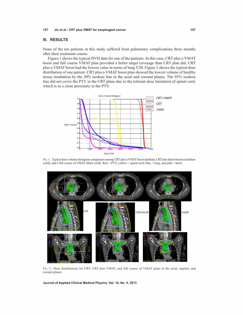
157 Jin et al.: CRT plus VMAT for esophageal cancer 157
Journal of Applied Clinical Medical Physics, Vol. 14, no. 5, 2013
III. RESuLTS
None of the ten patients in this study suffered from pulmonary complications three months after their treatment course.
Figure 1 shows the typical DVH data for one of the patients. In this case, CRT plus a VMAT boost and full course VMAT plan provided a better target coverage than CRT plan did. CRT plus a VMAT boost had the lowest value in terms of lung V20. Figure 2 shows the typical dose distribution of one patient. CRT plus a VMAT boost plan showed the lowest volume of healthy tissue irradiation by the 30% isodose line in the axial and coronal planes. The 95% isodose line did not cover the PTV in the CRT plans due to the tolerant dose limitation of spinal cord, which is in a close proximity to the PTV.
Fig. 1. Typical dose-volume histogram comparison among CRT plus a VMAT boost (dashed), CRT plus lateral beams (medium solid), and a full course of VMAT (thick solid). Red = PTV; yellow = spinal cord; blue = lung; and pink = heart.
Fig. 2. Dose distributions for CRT, CRT plus VMAT, and full course of VMAT plans in the axial, sagittal, and coronal planes.
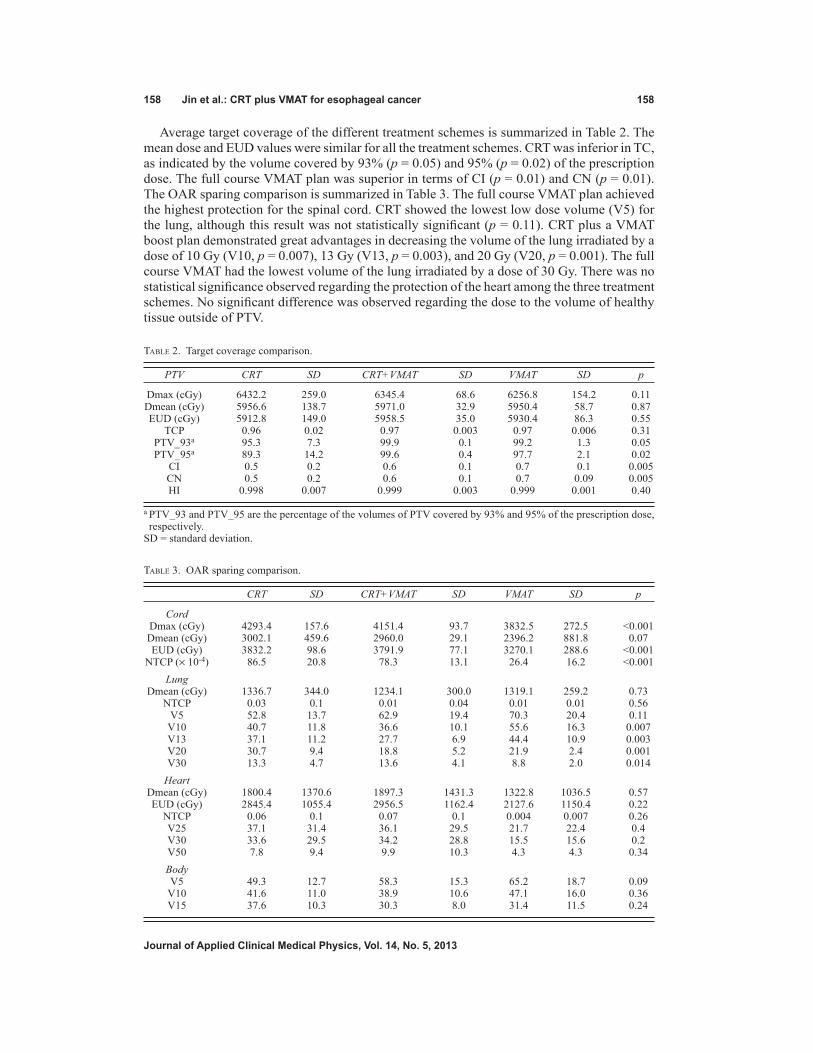
158 Jin et al.: CRT plus VMAT for esophageal cancer 158
Journal of Applied Clinical Medical Physics, Vol. 14, no. 5, 2013
Average target coverage of the different treatment schemes is summarized in Table 2. The mean dose and EUD values were similar for all the treatment schemes. CRT was inferior in TC, as indicated by the volume covered by 93% (p = 0.05) and 95% (p = 0.02) of the prescription dose. The full course VMAT plan was superior in terms of CI (p = 0.01) and CN (p = 0.01). The OAR sparing comparison is summarized in Table 3. The full course VMAT plan achieved the highest protection for the spinal cord. CRT showed the lowest low dose volume (V5) for the lung, although this result was not statistically significant (p = 0.11). CRT plus a VMAT boost plan demonstrated great advantages in decreasing the volume of the lung irradiated by a dose of 10 Gy (V10, p = 0.007), 13 Gy (V13, p = 0.003), and 20 Gy (V20, p = 0.001). The full course VMAT had the lowest volume of the lung irradiated by a dose of 30 Gy. There was no statistical significance observed regarding the protection of the heart among the three treatment schemes. No significant difference was observed regarding the dose to the volume of healthy tissue outside of PTV.
Table 2. Target coverage comparison.
PTV CRT SD CRT+VMAT SD VMAT SD p
Dmax (cGy) 6432.2 259.0 6345.4 68.6 6256.8 154.2 0.11 Dmean (cGy) 5956.6 138.7 5971.0 32.9 5950.4 58.7 0.87 EUD (cGy) 5912.8 149.0 5958.5 35.0 5930.4 86.3 0.55 TCP 0.96 0.02 0.97 0.003 0.97 0.006 0.31 PTV_93a 95.3 7.3 99.9 0.1 99.2 1.3 0.05 PTV_95a 89.3 14.2 99.6 0.4 97.7 2.1 0.02 CI 0.5 0.2 0.6 0.1 0.7 0.1 0.005 CN 0.5 0.2 0.6 0.1 0.7 0.09 0.005 HI 0.998 0.007 0.999 0.003 0.999 0.001 0.40
a PTV_93 and PTV_95 are the percentage of the volumes of PTV covered by 93% and 95% of the prescription dose, respectively.
SD = standard deviation.
Table 3. OAR sparing comparison.
CRT SD CRT+VMAT SD VMAT SD p
Cord Dmax (cGy) 4293.4 157.6 4151.4 93.7 3832.5 272.5 <0.001 Dmean (cGy) 3002.1 459.6 2960.0 29.1 2396.2 881.8 0.07 EUD (cGy) 3832.2 98.6 3791.9 77.1 3270.1 288.6 <0.001 NTCP (× 10-4) 86.5 20.8 78.3 13.1 26.4 16.2 <0.001 Lung Dmean (cGy) 1336.7 344.0 1234.1 300.0 1319.1 259.2 0.73 NTCP 0.03 0.1 0.01 0.04 0.01 0.01 0.56 V5 52.8 13.7 62.9 19.4 70.3 20.4 0.11 V10 40.7 11.8 36.6 10.1 55.6 16.3 0.007 V13 37.1 11.2 27.7 6.9 44.4 10.9 0.003 V20 30.7 9.4 18.8 5.2 21.9 2.4 0.001 V30 13.3 4.7 13.6 4.1 8.8 2.0 0.014 Heart Dmean (cGy) 1800.4 1370.6 1897.3 1431.3 1322.8 1036.5 0.57 EUD (cGy) 2845.4 1055.4 2956.5 1162.4 2127.6 1150.4 0.22 NTCP 0.06 0.1 0.07 0.1 0.004 0.007 0.26 V25 37.1 31.4 36.1 29.5 21.7 22.4 0.4 V30 33.6 29.5 34.2 28.8 15.5 15.6 0.2 V50 7.8 9.4 9.9 10.3 4.3 4.3 0.34 Body V5 49.3 12.7 58.3 15.3 65.2 18.7 0.09 V10 41.6 11.0 38.9 10.6 47.1 16.0 0.36 V15 37.6 10.3 30.3 8.0 31.4 11.5 0.24

159 Jin et al.: CRT plus VMAT for esophageal cancer 159
Journal of Applied Clinical Medical Physics, Vol. 14, no. 5, 2013
IV. dISCuSSIon
IMRT has shown to be superior to CRT in target coverage and normal tissue sparing in the treat-ment of esophageal cancer.(2) Studies have also indicated that VMAT is essentially equivalent to IMRT in the treatment of the esophagus from a dosimetric perspective.(10,17) In the present study, a single-arc VMAT boost plan following APPA conformal beams for upper thoracic esophageal cancer was demonstrated to be superior to the CRT in terms of better target coverage and the full course VMAT plan in terms of decreasing the lung volume irradiated by a low dose.
The cervical and upper esophageal areas lie in close proximity to the spinal cord. Drastic change in anatomical contours and diameters are often seen in upper thoracic esophageal cancer patients. The CTV of upper thoracic esophageal cancer usually includes the supraclavicular nodes at risk, and a part of the spinal cord may be projected inside the treatment field if lateral opposed beams or other off-cord conformal beams are applied during the boost phase. Because of this geometric difficulty, the dose coverage of the PTV usually had to be sacrificed in order to spare the spinal cord within its tolerant dose (45 Gy). This target coverage sacrifice is observed in our study. Using VMAT boost instead of off-cord conformal beams, the mean percent average target coverage of PTV (PTV_95) increased from 89.3 ± 14.2 to 99.6 ± 0.4 (p = 0.02). There was no significant difference (p = 0.87) in PTV_95 between CRT plus a sequential VMAT boost and the full course VMAT plan. The PTV_93 of CRT plus VMAT and full course of VMAT were also higher than that of CRT, but without statistical significance (p = 0.05). However, full course of VMAT plans demonstrated a higher CI (p = 0.01) and CN (p = 0.01) than did the other two treatment schemes, which is consistent with results of previous studies.(2,9) No significant difference was observed for HI (p = 0.4).
The spinal cord is one important organ with strict dose limitation. CRT plus a sequential VMAT boost plan achieved a relatively lower spinal cord NTCP (78.3 ± 13.1) than did CRT plans (86.5 ± 20.8), but no statistically significant differences were observed (p = 0.54). A clear spinal cord sparing advantage was found in full course of VMAT plans over CRT plans and CRT plus a sequential VMAT boost. The average maximum dose and EUD of the full course VMAT plans were about 461 cGy and 552 cGy less than those CRT plans, respectively (p < 0.001). The NTCP of the full course VMAT plans was nearly three times less than (p < 0.001) those of CRT and CRT plus a sequential VMAT boost. However, the maximum spinal cord doses in all three treatment schemes were within the tolerance level.
Pulmonary complications were another one of the major concerns associated with esopha-geal cancer radiotherapy. Several heterogeneous dosimetric parameters have been proposed to correlate with the incidence and severity of pneumonitis.(18-21) In this study, we compared these dosimetric parameters among these three planning schemes accordingly. There was no significant difference observed regarding the mean lung dose and NTCP among the three treatment schemes. The mean dose of the lung was considered to be the most useful predictor of radiation pneumonitis in thoracic tumor radiation in a study by Kwa et al.(18) On average, CRT plus off-cord conformal beams showed the lowest V5, but this difference was not sta-tistically significant (p = 0.11). V5 was also considered a strong indicator of pneumonitis in one postoperative chemoradiation study.(19) CRT plus a sequential VMAT boost demonstrated clear advantages in V10 (p = 0.007) and V13 (p = 0.003) compared with CRT plus off-cord conformal beams and full course of VMAT plans. V10 and V13 were also suggested to be strong indicators for pulmonary pneumonitis in a retrospective study.(20) CRT plus a sequential VMAT boost also showed the lowest value (p = 0.001) in lung V20, which was also found to be strongly correlated with the severity of pneumonitis.(20) Full course of VMAT plans presented a smallest value in V30, which also correlated to radiation pneumonitis in a study by Graham et al.(21) Although there is no single dosimetric parameter that is agreed to be the best predictor of radiation pneumonitis following radiotherapy, it is believed that lower volumes of the lung receiving intermediate and low-dose exposures are associated with better prognosis.(5) CRT

160 Jin et al.: CRT plus VMAT for esophageal cancer 160
Journal of Applied Clinical Medical Physics, Vol. 14, no. 5, 2013
plus a sequential VMAT boost demonstrated clear advantage in most of the lung dosimetric parameters in this study.
The lung sparing advantage associated with CRT plus a sequential VMAT boost is similar to the hybrid IMRT technique used in the study by Mayo et al.,(5) in which static conformal beams were concurrently combined with IMRT beams in the treatment of lung and esophageal cancer patients and were compared with CRT and IMRT. This result indicates that hybrid VMAT with APPA conformal beams concurrently combined with a single-arc VMAT beam may be a poten-tial technique in the treatment of esophageal cancer patients. However, this hybrid technique applying arc beam and conformal beams together in one fraction could increase the complexity of the planning process and beam delivery. Thus, applying VMAT only as the second boost phase is much more applicable and acceptable.
Full course of IMRT plans have been demonstrated to produce more conformal high-dose distributions to the PTV at the cost of low doses to more normal lung tissue.(22) Our study with full course of VMAT plans presented similar results. The full course VMAT plan achieved better target coverage and greater conformal dose distribution, as indicated by CI and CN, but a greater lung volume irradiated by the intermediate dose. Applying VMAT as only the second boost phase can reduce the volume of lung radiation compared to both CRT plus off-cord con-formal beams and the full course VMAT plan. At the same time, this method also improved the target coverage compared to CRT.
One potential problem with the full course VMAT plan is the increased volume of healthy tissue receiving low-dose radiation outside the PTV. In this study, conformal radiotherapy achieved the lowest V5 in healthy tissue, although with no statistical significance (p = 0.09). There was also no statistical significance for healthy tissue in V10 and V15. This result differs a little from that of the study of Vivekanandan et al.(9) They compared RapidArc (RA), CRT, and IMRT for ten esophageal cancer patients and found that V10 and integral dose to healthy tissue were similar for all the techniques; however, the RA plans resulted in a reduced low-level dose bath (15–20 Gy) in the range of 14%–16%, compared to the IMRT plans. The whole course VMAT plans demonstrated lower values on the heart parameters compared to CRT and CRT plus VMAT, but no significant differences (all p > 0.05) were observed regarding these parameters. This could also due to that heart was not involved in the inverse optimization.
V. ConCLuSIonS
Using APPA conformal beams plus a sequential VMAT boost for upper thoracic esophageal cancer can improve the target coverage compared to using CRT plus an off-cord conformal beams boost, while concurrently reducing the volume of the lung irradiated by the intermedi-ate dose. CRT combined with a sequential VMAT boost plan may be a promising treatment technique for upper thoracic esophageal cancer patients.
ACknowLEdgMEnTS
The study was supported by Wenzhou Science and Technology Bureau Funding (Y20120137) and the Scientific Research Foundation for the Returned Overseas Chinese Scholars (604090656/037).
REFEREnCES
1. Bradley JD and Muti S. Carcinoma of the esophagus. In: Levitt SH, Purdy JA, Perez CA, Vijayakumar S, editors. Technical basis of radiation therapy: practical clinical applications, 4th revised edition. Berlin: Springer; 2008: p.511–24.

161 Jin et al.: CRT plus VMAT for esophageal cancer 161
Journal of Applied Clinical Medical Physics, Vol. 14, no. 5, 2013
2. Fenkell L, Kaminsky I, Breen S, Huang S, Prooijen MV, Ringash J. Dosimetric comparison of IMRT vs. 3D con-formal radiotherapy in the treatment of cancer of the cervical esophagus. Radiother Oncol. 2008;89(3):287–91.
3. Palta JR, Deye JA, Ibbott GS, Purdy JA, Urie M. Credentialing of institutions for IMRT in the clinical trials. Int J Radiat Oncol Biol Phys. 2004;59(4):1257–59.
4. Advanced Technology Consortium. NCI guidelines on the use of IMRT in clinical trials. Accessed January 2007. Available from: http://atc.wustl.edu/home/NCI/NCI_IMRT_Guidelines.html
5. Mayo CS, Urie MM, Fitzgerald TJ, Ding L, Lo YC, Bogdanov M. Hybrid IMRT for treatment of cancers of the lung and esophagus. Int J Radiat Oncol Biol Phys. 2008;71(5):1408–18.
6. Bertelsen A, Hansen CR, Johansen J, Brink C. Single arc volumetric modulated arc therapy of head and neck cancer. Radiother Oncol. 2010;95(2):142–48.
7. Shaffer R, Morris WJ, Moiseenko V, et al. Volumetric modulated arc therapy and conventional intensity- modulated radiotherapy for simultaneous maximal intraprostatic boost: a planning comparison study. Clin Oncol. 2009;21(5):401–07.
8. Wolff D, Stierler F, Welzel G, et al. Volumetric intensity modulated arc therapy (VMAT) vs. serial tomotherapy, step-and-shot IMRT and 3D-conformal RT for treatment of prostate cancer. Radiother Oncol. 2009;93(2):226–33.
9. Vivekanandan N, Sriram P, Kumar S, Bhuvaneswari N, and Saranya K, Volumetric modulated arc radiotherapy for esophageal cancer. Med Dosim. 2012;37(1):108–13.
10. Van Benthuysen L, Hales L, Podgorsak MB. Volumetric modulated arc therapy vs. IMRT for the treatment of distal esophageal cancer. Med Dosim. 2011;36(4):404–09.
11. Radiation Therapy Oncology Group. RTOG 0436 A phase III trial evaluating the addition of cetuximab to pacli-taxel, cisplatin, and radiation for patients with esophageal cancer who are treated without surgery. Version date: 05/03/2012. Available from: http://www.rtog.org/ClinicalTrials/ProtocolTable/StudyDetails.aspx?study=0436
12. Wambersie A and Landber T. ICRU Report 62: Prescribing, recording, and reporting photon beam therapy. (Supplement to ICRU Report 50). Bethesda: ICRU; 1999.
13. Lomax NJ and Scheib SG. Quantifying the degree of conformity in radiosurgery treatment planning. Int J Radiat Oncol Biol Phys. 2003;55(5):1409–19.
14. van’t Riet A, Mak AC, Moerland MA, Elders LH, van der Zee W. A conformation number to quantify the degree of conformity in brachytherapy and external beam irradiation: application to the prostate. Int J Radiat Oncol Biol Phys. 1997;37(3):731–36.
15. Niemierko A and Goiten M. Modeling of normal tissue response to radiation: the critical volume model. Int J Radiat Oncol Biol Phys. 1993;25(1):135–45.
16. Okunieff P, Morgan D, Niemierko A, Suit HD. Radiation dose-response of human tumors. Int J Radiat Oncol Biol Phys. 1995;32(4):1227–37.
17. Hawkins MA, Bedford JL, Warrington AP, Tait DM. Volumetric modulated arc therapy planning for distal oesophageal malignancies. Br J Radiol. 2012;85(1009):44–52.
18. Kwa SL, Lebesque JV, Theuws JC, et al. Radiation pneumonitis as a function of mean lung dose: an analysis of pooled data of 540 patients. Int J Radiat Oncol Biol Phys. 1998;42(1):1–9.
19. Wang SL, Liao Z, Vaporciyan AA, et al. Investigation of clinical and dosimetric factors associated with postopera-tive pulmonary complications in esophageal cancer patients treated with concurrent chemoradiotherapy followed by surgery. Int J Radiat Oncol Biol Phys. 2006;64(3):692–99.
20. Lee HK, Vaporciyan AA, Cox JD, et al. Postoperative pulmonary complications after preoperative chemoradiation for esophageal carcinoma: correlation with pulmonary dose-volume histogram parameters. Int J Radiat Oncol Biol Phys. 2003;57(5):1317–22.
21. Graham MV, Purdy JA, Emami B, et al. Clinical dose-volume histogram analysis for pneumonitis after 3D treat-ment for non-small cell lung cancer (NSCLC). Int J Radiat Oncol Biol Phys. 1999;45(2):323–29.
22. Chapet O, Fraass BA, Ten Haken RK. Multiple fields may offer better esophagus sparing without increased prob-ability of lung toxicity in optimized IMRT of lung tumors. Int J Radiat Oncol Biol Phys. 2006;65(1):255–65.

a Corresponding author: Martina Descovich, University of California San Francisco Department of Radiation Oncology, 1600 Divisadero, Suite H1031, San Francisco, CA 94143-1708, USA; phone: (415) 353-9844; fax: (415) 353-9883; email: [email protected]
Improving plan quality and consistency by standardization of dose constraints in prostate cancer patients treated with CyberKnife
Martina Descovich,1a Mauro Carrara,2 Sara Morlino,3 Dilini S. Pinnaduwage,1 Daniel Saltiel,1 Jean Pouliot,1 Marc B. Nash,1 Emanuele Pignoli,2 Riccardo Valdagni,3 Mack Roach III,1 Alexander R. Gottschalk1
Department of Radiation Oncology,1 University of California San Francisco, San Francisco, CA, USA; Medical Physics Unit,2 Fondazione IRCCS, Istituto Nazionale dei Tumori, Milano, Italy; Radiotherapy 2 Unit and Prostate Cancer Program,3 Fondazione IRCCS Istituto Nazionale dei Tumori, Milano, [email protected]
Received 23 December, 2012; accepted 23 April, 2013
Treatment plans for prostate cancer patients undergoing stereotactic body radia-tion therapy (SBRT) are often challenging due to the proximity of organs at risk. Today, there are no objective criteria to determine whether an optimal treatment plan has been achieved, and physicians rely on their personal experience to evaluate the plan’s quality. In this study, we propose a method for determining rectal and bladder dose constraints achievable for a given patient’s anatomy. We expect that this method will improve the overall plan quality and consistency, and facilitate comparison of clinical outcomes across different institutions. The 3D proximity of the organs at risk to the target is quantified by means of the expansion-intersection volume (EIV), which is defined as the intersection volume between the target and the organ at risk expanded by 5 mm. We determine a relationship between EIV and relevant dosimetric parameters, such as the volume of bladder and rectum receiving 75% of the prescription dose (V75%). This relationship can be used to establish institution-specific criteria to guide the treatment planning and evaluation process. A database of 25 prostate patients treated with CyberKnife SBRT is used to validate this approach. There is a linear correlation between EIV and V75% of bladder and rectum, confirming that the dose delivered to rectum and bladder increases with increasing extension and proximity of these organs to the target. This information can be used during the planning stage to facilitate the plan optimization process, and to standardize plan quality and consistency. We have developed a method for determining customized dose constraints for prostate patients treated with robotic SBRT. Although the results are technology-specific and based on the experience of a single institution, we expect that the application of this method by other institu-tions will result in improved standardization of clinical practice.
PACS numbers: 87.55.-x, 87.55.D-, 87.55.de, 87.55.dk
Key words: prostate, stereotactic body radiation therapy, plan optimization, dose constraints
I. IntroduCtIon
The optimization and evaluation of a radiation therapy treatment plan is a complex process involving multiple steps. As a first step, the physician delineates target and organs at risk on the planning CT scan, often with the aid of other imaging sources (PET, MRI). Then the
JournAL oF APPLIEd CLInICAL MEdICAL PHYSICS, VoLuME 14, nuMBEr 5, 2013
162 162

163 descovich et al.: dose constraints for prostate SBrt 163
Journal of Applied Clinical Medical Physics, Vol. 14, no. 5, 2013
physicist or dosimetrist runs the computer-based optimization engine until a solution is found that meets the dosimetric parameters requested by the physician. The solution of the planning problem is particularly challenging when optimizing plans for prostate cancer patients treated with CyberKnife stereotactic body radiation therapy (SBRT). Multiple conflicting goals exist in this case, such as target coverage, conformity and homogeneity of the dose distribution, spar-ing of the organs at risks (bladder, rectum and urethra), and treatment time. Schlaefer et al.(1) describe a powerful multicriteria optimization approach for robotic radiosurgery. This method maps clinical goals into optimization steps and enables an optimal trade-off among different objectives by producing Pareto-efficient solutions.
As a next step physicist, dosimetrist, and physician visually examine the dose distribu-tion on the axial, sagittal, and coronal plane of the CT scan, and evaluate the target coverage and dose received by organs at risk using dose-volume histogram (DVH) analysis. A plan is deemed clinically acceptable if tumor coverage and dose tolerance to critical structures are within standard limits and/or meet physician expectations. The use of standard dose criteria in evaluating plan quality has however some limitations.(2) In particular, standard dose criteria do not account for the mutual disposition of target and organs at risk, which determines the difficulty of each individual treatment. In addition, modern radiotherapy equipment might provide superior dose distribution with lower dose to organs at risk, compared to conventional treatment modalities.
The main drawback of using equal dose criteria for every patient is that suboptimal treatment plans might still meet those criteria and, therefore, be deemed acceptable. Although physicist and physician experiences play a critical role in pushing the plan quality to the optimal limit, the process is somewhat subjective and lacks quantitative guidelines. Consequently, plans deemed acceptable might be far from the unknown optimality.
The goal of this study is to help establish an objective method to evaluate the plan’s quality, which accounts for the individual patient’s geometry and is independent of physician and plan-ner experiences. Prior to starting the optimization process, the method provides dose objectives for the individual case. These objectives are derived from a database of patients with similar characteristics and, therefore, can be considered achievable.
Differences in target and critical structures definition among physicians introduce a source of uncertainty in establishing a user independent quality control method based on geometric criteria. Previous studies reported significant differences in treatment planning and DVH analysis due to uncertainty in target(3) and critical structures contouring.(4)
In this work, we focus on prostate patients planned and treated with CyberKnife SBRT. However, a similar methodology can be developed for other treatment sites or treatment modalities.
The a priori knowledge of achievable dose constraints facilitates the treatment planning process and results in better plan quality. In addition, comparing dosimetric parameters of a newly developed treatment plan with institution-specific statistics provides a tool to control the plan quality and to improve the consistency among similar plans. We expect that this method will also facilitate interinstitution comparison of plan quality and eventually lead to standard-ization of clinical practice.
II. MAtErIALS And MEtHodS
The proposed method was developed for prostate patients treated with SBRT on the CyberKnife system (Accuray Inc., Sunnyvale, CA). In SBRT treatments, a high biologic-equivalent dose (BED) is delivered in few fractions (typically 2–5) with highly conformal distribution around the prostate and steep dose gradient at its periphery. Small treatment margins are possible, as the position of the prostate is monitored during the course of treatment every 30–60 seconds. Xie et al.(5) analyzed the intra-fraction prostate motion in 21 patients (105 fractions) treated with the CyberKnife system. They concluded that with an imaging interval of 30 seconds, target

164 descovich et al.: dose constraints for prostate SBrt 164
Journal of Applied Clinical Medical Physics, Vol. 14, no. 5, 2013
margins could be kept as low as 1 mm and that 2 mm margin would be required if the imaging interval was increased to 60 seconds. Gottschalk et al.(6) reported similar results.
Several SBRT treatment protocols are reported in the literature for the treatment of the prostate as both mono-therapy and post-pelvic irradiation boost.(7-10) The dose regimens and constraints for the organs at risk have been mainly derived from the experience in HDR brachytherapy, a well-established modality for delivering fewer high-dose fractions as monotherapy(11) or in combination with whole pelvis radiation therapy.(12) Table 1 reports a comparison of dose scheme and constraints published in the literature for HDR(13) and robotic SBRT protocols.(7-10)
In order to establish quality control criteria for treatment plan evaluation at our institution, we reviewed the dosimetric parameters obtained on a database of 25 prostate patients. For consistency in plan quality, we considered only plans generated with the Iris variable aperture collimator (Accuray Inc.), which enables to deliver multiple-size radiation fields at each robot position.(14) Iris treatments do not require physical collimator exchange and are delivered in a single path traversal. Previous studies have shown that plans generated with three collimator apertures deliver better treatment quality (improved dose conformity, homogeneity and/or cov-erage, and lower number of monitor units) compared to a single circular collimator.(14,15) The Iris collimator, therefore, offers the benefits of multiple-field-size treatments without increasing planning and delivery time.
The use of existing clinical plans of comparable treatment characteristics enabled us to determine dosimetric criteria that are achievable for a given patient anatomy.
The geometric distribution of organs at risk relative to the target plays a critical role in determining the achievable dose constraints. For example, standard dose criteria can be easily achieved for a patient with a small prostate and a large separation between target and organs at risk (Fig. 1, left). On the other hand, it is very difficult to achieve the same dose constraints in a patient with a large prostate and significant interface between target and organs at risk (Fig. 1, right). Treatment preparation, such as rectum and bladder filling, and the use of rectal balloons (for prostate immobilization and rectal wall sparing), bladder catheters (for constant bladder filling), and Foley catheters (for urethral delineation) influence the patient geometry and organ disposition. At our institution, patients are simulated with empty rectum and bladder (due to the prolonged treatment time, it is not feasible for the patients to maintain full bladder). In addition, the use of endorectal coils during MRI acquisition, and Foley catheters during simulation or treatment is not allowed to prevent deformation in the prostate gland.
In order to quantify the geometric relationship in the 3D space between the target volume and the organs at risk we used the concept of expansion-intersection histogram proposed by
Table 1. Literature-based treatment parameters for HDR and robotic SBRT protocols.
Parameter HDR(13) San Diego(8) UCSF(9) Erasmus(7) UCLA(10)
Total dose 19 Gy 38 Gy 19 or 38 Gy 38 Gy 36.25 Gy Fractions 2 4 2 or 4 4 5 Prescription >50% >60% >67% 88%-92% PTV margin none 2-5 mm/0 post. 2 mm/0 post. 3 mm/0 post. 5 mm/3 mm post. PTV V100%a ≥90% V100%a ≥95% V100%a ≥95% V100%a ≥95% V100%a ≥95% Rectum V75%a <1 cc Wall V100%a = 0 V75%a <2 cc Wall V100%a = 0 V50%a <50% V80%a <20% Mucosab V75%a = 0 Mucosab V75%a = 0 V90%a <10% V85%a <1 cc V100%a <5% Bladder V75%a <1 cc V120%a = 0 V75%a <3 cc V110%a = 0 V50%a <40% V100%a <1 cc V100%a <10% Urethra V125%a <1 cc V120%a = 0 V120%a <10% V120%a = 0
a Vxx: Volume of structure (PTV or organ at risk) receiving xx% of prescription dose.b Mucosa: solid structure formed by a 3 mm contraction of the rectal wall.

165 descovich et al.: dose constraints for prostate SBrt 165
Journal of Applied Clinical Medical Physics, Vol. 14, no. 5, 2013
Tomatis et al.(16) We define the intersection volume between the target and the organ at risk expanded by 5 mm as EIV, expansion-intersection volume. A large EIV indicates that a large area of organ at risk faces the target, leading to a more difficult plan optimization.
A. treatment planning techniqueFor each patient, three gold fiducial markers are implanted into the prostate gland at least one week prior to CT simulation. The gold markers provide a reference frame to localize the posi-tion of the prostate in the X-ray images acquired during treatment. A CT scan using 1.5 mm slice thickness is acquired, together with T1- and T2-weighted MRI imaging sequences. The CT and T2-weighted MRI scans are coregistered using a point-based registration to match the fiducial location. While the T2 sequence provides optimal visibility of prostate and urethra, the T1 sequence helps identify the fiducial markers, which produce a low signal in the T2-weighed images. The planning target volume (PTV) is created by a uniform 2 mm expansion of the prostate (contoured on the T2 sequence), except posteriorly to protect the rectum. The physi-cian also contours organs at risk such as bladder, rectum, urethra, penis, testicles, bowel, and femoral heads. All organs at risk, except the urethra, are contoured on the planning CT. The bladder is contoured from its base to the dome. The rectum is contoured from the anus to the recto-sigmoid flexure.
The “sequential optimization” (or “stepwise optimization”) method is used for plan genera-tion.(1) This method provides a flexible approach to solve the planning problem and optimize multiple conflicting goals reproducing the decision-making process of a clinician. Unlike inverse planning algorithms, which use relative weights and a single mathematical function to optimize all planning goals at once, sequential optimization addresses each goal separately in a predefined order. After each step, the feasibility of the solution is retained or relaxed by a user-defined value to improve plan quality at the next step. However, in the CyberKnife implementation of the sequential method, the relaxation parameter applies only to the last step in the sequential chain. This prevents major improvements in plan quality after step 2. The sequential optimization method possesses the right characteristics for scripting. Scripts (or plan templates) greatly reduce the variability of different treatment planning skills and help improve the standardization among similar plans.
For prostate patients, a planning template is used at our institution. Beams intersecting the testicles are disabled, and field sizes ranging from the largest aperture that fits the PTV con-tour down to the 12.5 mm diameter opening are selected. Three asymmetric shells are created
Fig. 1. Anatomy of prostate patients. Examples of favorable (left) and unfavorable (right) patient anatomy for a prostate SBRT treatment. Linear dimensions of bladder-PTV and rectum-PTV interface are displayed on the same scale.

166 descovich et al.: dose constraints for prostate SBrt 166
Journal of Applied Clinical Medical Physics, Vol. 14, no. 5, 2013
around the PTV with larger margins in the lateral direction and tighter margins in the anterior–posterior direction, to improve rectum and bladder sparing. Shells are tuning structures used by the optimization algorithm to achieve a conformal dose distribution around the target and control the dose gradient at its periphery. The distance between shell and PTV is 1–4 mm for the first shell, 6–12 mm for the second shell, and 15–25 mm for the third shell. The use of thin shells and dose-volume constraints for planning robotic radiosurgery is reported in the paper by Schlaefer et al.(17) This article discusses a specific example for a prostate case.
A maximum of 200 monitor units (MUs) per beam per fraction is set in order to limit the beam-on time from each direction, therefore preventing a “finger-like” dose distribution. The dose distribution has “fingers” when the isodose line corresponding to 50% of the prescription dose is not shaped around the target, but protrudes for several centimeters away from it. Properly placed shells also help reducing this effect. The maximum MU per node is set to be slightly larger than the maximum MU per beam to enable the use of multiple beams per node, while avoiding skin hotspots due to predominant beam entry points. In some cases, the definition of a planning-specific target that does not overlap with bladder and rectum, and does not include the urethra, facilitates the planning process.
The sequential optimization script is run to achieve the following clinical goals: i) to cover 95% of PTV with 100% of the prescription dose; ii) to keep the volume of urethra receiving 120% of the prescription dose (V120%) less than 0.1 cc; iii) to minimize the volume of rectum receiving 75% of the prescription dose (V75%); iv) to minimize the volume of bladder receiving 75% of the prescription dose (V75%); and v) to obtain a dose distribution highly conformal around the target, with no hot spots in normal tissue.
After a plan of acceptable quality is achieved, beam and time reduction tools are used to obtain the best compromise between treatment efficiency and dosimetric quality.(18)
B. training cohortEleven of the 25 patients in the training cohort were treated with SBRT monotherapy using a dose of 38 Gy in 4 fractions. Fourteen patients were treated with SBRT boost. Among these, seven patients received a dose of 19 Gy in 2 fractions and seven patients received a dose of 21 Gy in 2 fractions, according to a dose escalation protocol. To assess the robustness of the method to contouring uncertainties, patients contoured by three physicians were included in our study. Two physicists were involved in the treatment planning process.
The average PTV volume is 58.3 cm3 (range 11.3–148.3 cm3), the average bladder volume is 130.8 cm3 (range 47.8–385.5 cm3), and the average rectum volume is 102.0 cm3 (range 45.4–365.8 cm3). For all plans, target coverage ≥ 95%, and prescription isodose-line > 60% are achieved. The average number of beams is 209 (range 112–360), and the average treatment time (excluding setup time) is 43 minutes (range 27–60 minutes).
For each plan, the following parameters are recorded and analyzed: i) EIV of rectum and bladder; ii) V75% of rectum and bladder; iii) V120% of urethra; iv) conformity index (nCI).
The conformity index describes how well the prescription isodose volume (PIV) conforms to the target volume (TV) and it is defined as: nCI = TV × PIV / (TIV)2, where TIV is the target volume inside the prescription isodose volume. The average nCI was 1.24 (range 1.14–1.41), and the average urethra V120 was 0.03 cc (range 0–0.19 cc).
In this analysis, we use V75% of bladder and rectum and V120% of urethra as the key dosimetric parameters to evaluate plan quality. This choice reflects our clinical practice and is based on the experience with HDR brachytherapy.(12)
The V75% values of bladder and rectum are plotted as a function of the EIV values of bladder and rectum. A linear regression analysis is performed in order to model the relationship between these two parameters. Prediction intervals, representing the intervals where 90% and 95% of future observations will fall, are also calculated. The prediction intervals enable to compare a new plan to our institutional standards and provide a method for quality control.
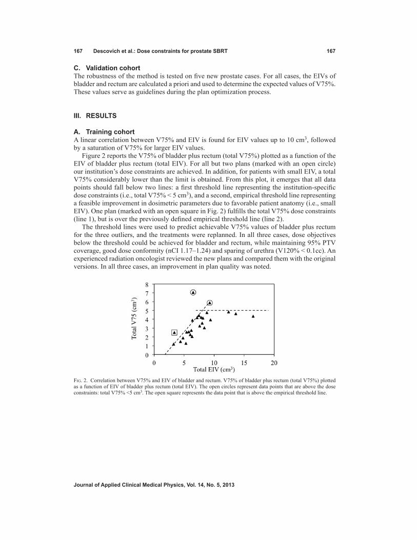
167 descovich et al.: dose constraints for prostate SBrt 167
Journal of Applied Clinical Medical Physics, Vol. 14, no. 5, 2013
C. Validation cohortThe robustness of the method is tested on five new prostate cases. For all cases, the EIVs of bladder and rectum are calculated a priori and used to determine the expected values of V75%. These values serve as guidelines during the plan optimization process.
III. rESuLtS
A. training cohortA linear correlation between V75% and EIV is found for EIV values up to 10 cm3, followed by a saturation of V75% for larger EIV values.
Figure 2 reports the V75% of bladder plus rectum (total V75%) plotted as a function of the EIV of bladder plus rectum (total EIV). For all but two plans (marked with an open circle) our institution’s dose constraints are achieved. In addition, for patients with small EIV, a total V75% considerably lower than the limit is obtained. From this plot, it emerges that all data points should fall below two lines: a first threshold line representing the institution-specific dose constraints (i.e., total V75% < 5 cm3), and a second, empirical threshold line representing a feasible improvement in dosimetric parameters due to favorable patient anatomy (i.e., small EIV). One plan (marked with an open square in Fig. 2) fulfills the total V75% dose constraints (line 1), but is over the previously defined empirical threshold line (line 2).
The threshold lines were used to predict achievable V75% values of bladder plus rectum for the three outliers, and the treatments were replanned. In all three cases, dose objectives below the threshold could be achieved for bladder and rectum, while maintaining 95% PTV coverage, good dose conformity (nCI 1.17–1.24) and sparing of urethra (V120% < 0.1cc). An experienced radiation oncologist reviewed the new plans and compared them with the original versions. In all three cases, an improvement in plan quality was noted.
Fig. 2. Correlation between V75% and EIV of bladder and rectum. V75% of bladder plus rectum (total V75%) plotted as a function of EIV of bladder plus rectum (total EIV). The open circles represent data points that are above the dose constraints: total V75% <5 cm3. The open square represents the data point that is above the empirical threshold line.

168 descovich et al.: dose constraints for prostate SBrt 168
Journal of Applied Clinical Medical Physics, Vol. 14, no. 5, 2013
Figure 3 is an update of Fig. 2, where the data for the three outliers are replaced with the replanned data (marked as open circles). A regression analysis for the data points with EIV < 10 cm3 provides a reasonable linear correlation (R2 = 0.76) between the total V75% and EIV. The 90% and 95% prediction intervals are also displayed. For data points with EIV > 10 cm3, the horizontal threshold line representing the institution-specific dose constraints (total V75% < 5 cm3) provides the method for quality control, and the prediction intervals are not calculated.
Fig. 3. Correlation between V75% and EIV of bladder and rectum — re-optimized plans. V75% of bladder plus rectum (total V75%) plotted as a function of EIV of bladder plus rectum (total EIV). Correlation line and prediction intervals are displayed. The open circles represent data for the re-optimized treatment plans.

169 descovich et al.: dose constraints for prostate SBrt 169
Journal of Applied Clinical Medical Physics, Vol. 14, no. 5, 2013
B. Validation cohortFor all new prostate cases, it was possible to obtain clinically acceptable plans with (total EIV, total V75%) coordinates falling within the prediction intervals. Figure 4 displays the location of the new data points (open squares) in the (total EIV, total V75%) graph. The a priori knowledge of achievable V75% values facilitates the treatment planning process. Plans were generated by a physicist specialized in robotic radiosurgery planning in less than one day.
IV. dISCuSSIon
We presented an objective method, based on clinical experience, to evaluate the quality and consistency of prostate SBRT plans. This method enables to determine whether a satisfactory plan has been obtained without relying on personal experience. In our definition, a satisfac-tory plan meets the clinical goals in terms of target coverage, organs at risk sparing, and dose conformity, and therefore is consistent with the clinical objectives at our institution.
The linear correlation between EIV and V75% of bladder and rectum confirms that the dose delivered to bladder and rectum increases with increasing extension of the organs area fac-ing the target. For a given EIV value, the linear fit enables to determine a priori optimal dose objectives for the organs at risk. This knowledge facilitates the treatment planning process in terms of both planning efficiency and plan quality, and provides a means to detect abnormal plan behavior.
In our analysis, the dose objectives for bladder and rectum are combined in a single param-eter, the total V75%. The correlation between the total V75% and total EIV is indeed stronger than the correlation between V75% and EIV of bladder and rectum analyzed separately. This behavior can be explained by considering possible geometrical mutual dispositions of prostate and organs at risk, as displayed in Fig. 5. In the schematic drawings (Fig. 5(a) to 5(d)), prostate, bladder and rectum have the same size, but different mutual disposition. In Fig. 5(a), bladder and rectum are far from the prostate and therefore their EIVs are small; in (b) bladder EIV is large and rectum EIV is small; in (c) bladder EIV is small and rectum EIV is large; in (d) both organs are facing the prostate and therefore their EIVs are large. In Figs. 5(b) and (c), the treat-ment plan can be optimized so that the 5% fraction of PTV volume receiving less than 100% of the prescribed dose (acceptable PTV coverage is 95%) is entirely concentrated at the interface with the bladder or with the rectum, respectively. In this way, the portion of bladder or rectum facing the prostate is mostly spared because the dose gradient starts already inside the prostate. Conversely, in Fig. 5(d) both organs at risk are facing the target, and a compromise for the loca-tion of the dose gradient has to be reached. Figure 5 demonstrates that the dose delivered to the
Fig. 4. Correlation between V75% and EIV of bladder and rectum — validation data. V75% of bladder plus rectum (total V75%) plotted as a function of EIV of bladder plus rectum (total EIV). The open squares represent the validation data.

170 descovich et al.: dose constraints for prostate SBrt 170
Journal of Applied Clinical Medical Physics, Vol. 14, no. 5, 2013
rectum depends not only on its proximity to the target, but also on the proximity of the bladder to the target. Similarly, the dose delivered to the bladder depends on the rectum location.
In the optimization algorithm, user-defined dose constraints are set in order to minimize the dose delivered to bladder and rectum. By properly adjusting constraints and optimization steps in the sequential workflow, it is possible to either balance the V75% of bladder and rectum to a similar value, or to prioritize the sparing of one organ versus the other, depending on the detailed clinical assessment.
The total EIV analysis returns the value of V75% of bladder plus rectum for a given patient anatomy. The achievable V75% of rectum and bladder, separately, can be estimated as follows:
Bladder V75% = f * Total V75% (1) Rectum V75% = (1-f) * Total V75% (2)
where f is a parameter with values ranging between 0 and 1. In general, f = 0.5 can be used. However, for large EIV it is generally preferred to keep rectum V75% < 2 cm3 and bladder V75% < 3 cm3. In this case, f = 0.6 is used.
A similar interplay is observed between the sparing of the organs at risk and the dose con-formity around the target. Figure 6 shows the total V75% versus the total EIV separated in two groups: 1) plans with nCI < 1.25 (black triangles), and 2) plans with nCI ≥ 1.25 (open squares). A slightly stronger linear correlation between V75% and EIV emerges from the two groups (R2 = 0.83 and R2 = 0.77 for plans with low nCI and high nCI, respectively). Two almost par-allel correlation lines are obtained from the two datasets, demonstrating that for a given EIV value, there are two alternative approaches to optimize the V75% values, one corresponding to a more conformal plan (nCI < 1.25) and one corresponding to a less conformal plan (nCI ≥ 1.25). Although some differences are observed between the linear fits for the different conformity levels, these results are not statistically significant. Prioritizing dose conformity, sparing of bladder and sparing of rectum is a clinical decision that needs to be evaluated on a case-by-case basis. For patients with favorable anatomy, physicians may also consider escalating the dose,
Fig. 5. Geometrical disposition of prostate and organs at risk.
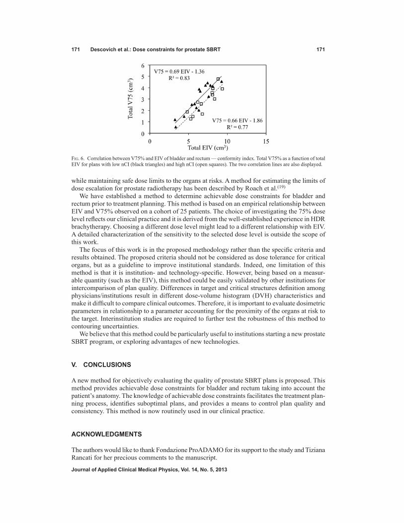
171 descovich et al.: dose constraints for prostate SBrt 171
Journal of Applied Clinical Medical Physics, Vol. 14, no. 5, 2013
while maintaining safe dose limits to the organs at risks. A method for estimating the limits of dose escalation for prostate radiotherapy has been described by Roach et al.(19)
We have established a method to determine achievable dose constraints for bladder and rectum prior to treatment planning. This method is based on an empirical relationship between EIV and V75% observed on a cohort of 25 patients. The choice of investigating the 75% dose level reflects our clinical practice and it is derived from the well-established experience in HDR brachytherapy. Choosing a different dose level might lead to a different relationship with EIV. A detailed characterization of the sensitivity to the selected dose level is outside the scope of this work.
The focus of this work is in the proposed methodology rather than the specific criteria and results obtained. The proposed criteria should not be considered as dose tolerance for critical organs, but as a guideline to improve institutional standards. Indeed, one limitation of this method is that it is institution- and technology-specific. However, being based on a measur-able quantity (such as the EIV), this method could be easily validated by other institutions for intercomparison of plan quality. Differences in target and critical structures definition among physicians/institutions result in different dose-volume histogram (DVH) characteristics and make it difficult to compare clinical outcomes. Therefore, it is important to evaluate dosimetric parameters in relationship to a parameter accounting for the proximity of the organs at risk to the target. Interinstitution studies are required to further test the robustness of this method to contouring uncertainties.
We believe that this method could be particularly useful to institutions starting a new prostate SBRT program, or exploring advantages of new technologies.
V. ConCLuSIonS
A new method for objectively evaluating the quality of prostate SBRT plans is proposed. This method provides achievable dose constraints for bladder and rectum taking into account the patient’s anatomy. The knowledge of achievable dose constraints facilitates the treatment plan-ning process, identifies suboptimal plans, and provides a means to control plan quality and consistency. This method is now routinely used in our clinical practice.
ACKnowLEdgMEntS
The authors would like to thank Fondazione ProADAMO for its support to the study and Tiziana Rancati for her precious comments to the manuscript.
Fig. 6. Correlation between V75% and EIV of bladder and rectum — conformity index. Total V75% as a function of total EIV for plans with low nCI (black triangles) and high nCI (open squares). The two correlation lines are also displayed.

172 descovich et al.: dose constraints for prostate SBrt 172
Journal of Applied Clinical Medical Physics, Vol. 14, no. 5, 2013
rEFErEnCES
1. Schlaefer A and Schweikard A. Stepwise multi-criteria optimization for robotic radiosurgery. Med Phys. 2008;35(5):2094–103.
2. Ruan D, Shao W, Demarco J, et al. Evolving treatment plan quality criteria from institution-specific experience. Med Phys. 2012;39(5):2708–12.
3. Fiorino C, Reni M, Bolognesi A, Cattaneo GM, Calandrino R. Intra- and inter-observer variability in con-touring prostate and seminal vesicles: implications for conformal treatment planning. Radiother Oncol. 1998;47(3):285–292.
4. Foppiano F, Fiorino C, Frezza G, et al. The impact of contouring uncertainty on rectal 3D dose-volume data: Results of a dummy run in a multicenter trial (AIROPROS01-02). Int J Radiat Oncol Biol Phys. 2003;57(2):573–79.
5. Xie YQ, Djajaputra D, King CR, Hossain S, Ma L, Xing L. Intrafractional motion of the prostate during hypof-ractionated radiotherapy. Int J Radiat Oncol Biol Phys. 2008;72(1):236–46.
6. Gottschalk AR, Hossain S, Chuang C, Descovich M, Ma L. Intrafraction prostate motion during CyberKnife radiosurgery: implications on planning margins [abstract]. Int J Radiat Oncol Biol Phys. 2008;72(1):S569.
7. Aluwini S, van Rooij P, Hoogeman M, et al. CyberKnife stereotactic radiotherapy as monotherapy for low- to intermediate-stage prostate cancer: early experience, feasibility, and tolerance. J Endourol. 2010;24(5):865–69.
8. Fuller DB, Naitoh J, Lee C, Hardy S, Jin H. Virtual HDR CyberKnife treatment for localized prostatic carcinoma: dosimetry comparison with HDR brachytherapy and preliminary clinical observations. Int J Radiat Oncol Biol Phys. 2008;70(5):1588–97.
9. Jabbari S, Weinberg VK, Kaprealian T, et al. Stereotactic body radiotherapy as monotherapy or post-external beam radiotherapy boost for prostate cancer: technique, early toxicity, and PSA response. Int J Radiat Oncol Biol Phys. 2012;82(1):228–34.
10. King CR, Brooks JD, Gill H, Presti JC, Jr. Long-term outcomes from a prospective trial of stereotactic body radiotherapy for low-risk prostate cancer. Int J Radiat Oncol Biol Phys. 2012;82(2):877–82.
11. Barkati M, Williams SG, Foroudi F, et al. High-dose-rate brachytherapy as a monotherapy for favorable-risk prostate cancer: a Phase II trial. Int J Radiat Oncol Biol Phys. 2012;82(5):1889–96.
12. Hsu IC, Bae K, Shinohara K, et al. Phase II trial of combined high-dose-rate brachytherapy and external beam radiotherapy for adenocarcinoma of the prostate: preliminary results of RTOG 0321. Int J Radiat Oncol Biol Phys. 2010;78(3):751–58.
13. Hsu IC. Phase II Trial of combined high dose rate brachytherapy and external beam radiotherapy for adenocar-cinoma of the prostate. RTOG 0321. Philadelphia, PA: Radiation Therapy Oncology Group, 2006.
14. Echner GG, Kilby W, Lee M, et al. The design, physical properties and clinical utility of an iris collimator for robotic radiosurgery. Phys Med Biol. 2009;54(18):5359–80.
15. Poll JJ, Hoogeman MS, Prevost JB, Nuyttens JJ, Levendag PC, Heijmen BJ. Reducing monitor units for robotic radiosurgery by optimized use of multiple collimators. Med Phys. 2008;35(6):2294–99.
16. Tomatis S, Carrara M, Massafra E, et al. Geometry of volumes in radiotherapy planning. A new method for a quantitative assessment. Tumori. 2011;97(4):503–09.
17. Schlaefer A, Ruan D, Dieterich S, and Kilby W. Linear implementation of dose-volume constraints for multi-criteria optimization. In: IFMBE Proceedings, World Congress on Medical Physics and Biomedical Engineering. Doessel O and Schlegel WC, editors. Munich, Germany, 7-12 September 2009. Berlin: Springer; 2009. p. 321.
18. Kilby W, Dooley JR, Kuduvalli G, Sayeh S, Maurer CR, Jr. The CyberKnife Robotic Radiosurgery System in 2010. Technol Cancer Res Treat. 2010;9(5):433–52.
19. Roach M, 3rd, Pickett B, Weil M, Verhey L. The “critical volume tolerance method” for estimating the limits of dose escalation during three-dimensional conformal radiotherapy for prostate cancer. Int J Radiat Oncol Biol Phys. 1996;35(5):1019–25.

a Corresponding author: Masashi Yagi, Department of Radiation Oncology, Osaka University Graduate School of Medicine, 2-2 (D10) Yamada-oka, Suita, Osaka, 5650871, Japan; phone: +81-6-6879-3482; fax: +81-6-6879-3489; email: [email protected]
Gemstone spectral imaging: determination of CT to ED conversion curves for radiotherapy treatment planning
Masashi Yagi,1a Takashi Ueguchi,2 Masahiko Koizumi,3 Toshiyuki Ogata,1 Sachiko Yamada,2 Yutaka Takahashi,1 Iori Sumida,4 Yuichi Akino,1 Koji Konishi,1 Fumiaki Isohashi,1 Noriyuki Tomiyama,5 Yasuo Yoshioka,1 Kazuhiko Ogawa1
Department of Radiation Oncology,1 Osaka University Graduate School of Medicine, Osaka; Department of Radiology,2 Osaka University Hospital, Osaka; Division of Medical Physics,3 Oncology Center, Osaka University Hospital, Osaka; Department of Oral and Maxillofacial Radiology,4 Osaka University Graduate School of Dentistry, Osaka; Department of Diagnostic and Interventional Radiology,5 Osaka University Graduate School of Medicine, Osaka, [email protected]
Received 27 December, 2012; accepted 9 April, 2013
The monochromatic images acquired by Gemstone spectral imaging (GSI) mode on the GE CT750 HD theoretically determines the computed tomography (CT) number more accurately than that of conventional scanner. Using the former, the CT number is calculated from (synthesized) monoenergetic X-ray data. We rea-soned that the monochromatic image might be applied to radiotherapy treatment planning (RTP) to calculate dose distribution more accurately. Our goal here was to provide CT to electron density (ED) conversion curves with monochromatic images for RTP. Therefore, we assessed the reproducibility of CT numbers, an important factor on quality assurance, over short and long time periods for different substances at varying energy. CT number difference between measured and theoreti-cal value was investigated. The scanner provided sufficient reproducibility of CT numbers for dose calculation over short and long time periods. The CT numbers of monochromatic images produced by this scanner had reasonable values for dose calculation. The CT to ED conversion curve becomes linear with respect to the relationship between CT numbers and EDs as the energy increases. We conclude that monochromatic imaging from a fast switching system can be applied for the dose calculation, keeping Hounsfield units (HU) stability.
PACS numbers: 87.55.-x, 87.55.ne, 87.57.N-, 87.59.bd
Key words: dual-energy CT, Gemstone spectral imaging, monochromatic image, radiotherapy treatment planning, CT to ED conversion curve
I. InTroDuCTIon
The application of computed tomography (CT) in radiotherapy is growing and plays an important role for radiotherapy. In radiotherapy, the information acquired by the CT scanner is mainly used to identify targets and organs at risk (OARs) and determine appropriate dosing.(1)
Recently, dual-energy CT has been commercially available. The dual-energy CT concept was suggested by Hounsfield in 1973.(2) Technological limits such as low rotation speed made it initially difficult to use the scanner clinically. However, subsequent rapid advances in CT technology have resulted in the ubiquitous clinical presence of dual-energy scanners. Dual-energy CT can provide more valuable information such as effective atomic number, electron
JournAL oF APPLIED CLInICAL MEDICAL PHYSICS, VoLuME 14, nuMBEr 5, 2013
173 173

174 Yagi et al.: Gemstone spectral imaging for rTP 174
Journal of Applied Clinical Medical Physics, Vol. 14, no. 5, 2013
density, and mass density(3,4,5) than that acquired by conventional scanners. Furthermore, the monochromatic X-ray image acquired by the dual-energy scanner theoretically yields more accurate data than that of the conventional scanner because the theory (details in the paragraph below) predicts the elimination of spectral beam hardening artifacts.(5,6,7) We reasoned that the monochromatic image could make more accurate dose distribution calculations when applied to radiotherapy treatment planning (RTP). Therefore, we set out to validate this technique.
There are three types of dual-energy CT acquisition systems commercially available: Toshiba (Toshiba Corporation, Tokyo, Japan) with one tube and two rotations, Siemens(8) (Siemens Medical Solutions, Malvern, PA, USA) with two tubes and one rotation, and GE(9) (GE Healthcare, Waukesha, WI, USA) with one tube one rotation called a fast switching system. The similar system to that from GE is described in several papers.(7,10,11) One of the most important requirements for the success of dual-energy CT scanning is that there should be minimal time delay between the two acquisitions of the two single energy projection/images. We utilize a Discovery CT750 HD (GE Healthcare). In the GE system, fast rotation speed (0.5–1 s), use of X-ray focal spot deflection, fast voltage switching speed between 80 and 140 kVp in less than 0.5 ms, and a newly developed cerium activated garnet rare-earth composite scintillator detector with 100 times faster response than a typical gadolinium oxysulfide CT detector allow us to perform successful dual-energy CT acquisition.
The basic theory of this algorithm was first reported by Alvarez and Macovski(6) and studied extensively by others.(12,13) The system uses a dual-energy pre-reconstruction algorithm for creating synthesized monochromatic CT image from the material density images. The fol-lowing is an explanation of the method.(7,9) The basic assumption underlying this algorithm is that over the diagnostic X-ray energy range, the explicitly energy-dependent linear attenuation coefficient of all materials can be expressed with sufficient accuracy as a linear combination of photoelectric and Compton coefficients.(6) In direct consequence, the linear attenuation coef-ficient in each voxel of CT image at energy, E, is given by:
(1)
where μL(E) is linear attenuation coefficient in each voxel at X-ray energy E (in kVp), and dα and dβ are the dual-energy CT determined densities or concentrations of basis materials α and β at the voxel location, respectively. Thus, the information of two materials is needed to calculate the linear attenuation coefficient. It should be sufficiently different in their atomic number Z and in their photoelectric and Compton attenuation characteristics to distinguish the two materials. μM(E)α and μM(E)β are the mass attenuation coefficients of material α and β. In CT, the line integral over the linear attenuation coefficient is determined for each focus position and detector element, respectively. This integral can be expressed accordingly as:
(2)
where
(3)
δi is the area density in g/cm2 and di(r) is the local density in g/cm3 of the basis material i.

175 Yagi et al.: Gemstone spectral imaging for rTP 175
Journal of Applied Clinical Medical Physics, Vol. 14, no. 5, 2013
The equivalent area densities, δα and δβ, are determined for each ray path in projections. This problem is solved by measuring the attenuation with two different energies (spectra). Because the X-ray attenuates according to Beer-Lambert law (i.e., exponential attenuation law):
(4)
where I and I0 are the attenuated and primary intensities, two nonlinear equations for each path are derived:
(5)
(6)
The subscripts h and l refer to the high- and low-kVp energy. Eqs. (5) and (6) can be solved for the equivalent area densities, δα and δβ.
Since mass attenuation coefficient would have been measured with a mono-energetic X-ray source,(14) once the equivalent area densities are determined, the projection data can be cal-culated. This is done by multiplying the known area density values by the mass attenuation coefficients of the respective basis materials for an arbitrary mono-energy E0 (in keV):
(7)
where μM(E0)i are taken from Storm and Israel.(14) The projection data are then subjected to the standard reconstruction process yielding CT images in Hounsfield units (HU).(15)
In conventional CT, the HU or CT number (CT#) is computed as:
(8)
where μL(E)w is the linear attenuation of pure water at a given energy E. In dual-energy CT, to calculate CT# at E0, the equation is transformed using the linear mass relationship μL = ρμM and substituted Eq. (1) into Eq. (8):
(9)
where ρw and μM(E0)w are the pure water mass density and mass attenuation coefficient of pure water at energy E0, respectively. This monochromatic image synthesis workflow is implemented in Gemstone spectral imaging (GSI) mode while standard polychromatic images were obtained using the regular operation mode.
The goal of this study is to provide CT to ED (electron density) conversion curves derived from dual-energy CT monochromatic images for RTP. The CT number accuracy, as well as the repro-ducibility of CT numbers (an important factor on quality assurance), was also investigated.

176 Yagi et al.: Gemstone spectral imaging for rTP 176
Journal of Applied Clinical Medical Physics, Vol. 14, no. 5, 2013
II. MATErIALS AnD METHoDS
A. PhantomA tissue characterization phantom (Gammex RMI 467, Gammex RMI, Middleton, WI, USA) with 33 cm in diameter and 5 cm in height was used. The rods’ compositions mimicked those of human body organs with known electron densities relative to water, ranging from low (e.g., air) to high (e.g., bone). The phantom was composed mainly of solid water. In radiotherapy, this phantom is commonly used to establish EDs of various tissues and their corresponding CT numbers (in Hounsfield units, HU) for accurate corrections for tissue heterogeneity. Table 1 summarizes the physical characteristics of the rods (provided by the manufacturer to compen-sate slight differences among products). Correctly aligning rods is quite important because high-density rods cause artifacts that affect the accuracy of the CT numbers. Therefore, rods were inserted into the phantom according to the manufacture’s recommendations (Tissue Characterization Phantom Model 467 User’s Guide).(16) Figure 1 shows the distribution of the rods used in this study.
Table 1. Physical characteristics of rods. The data are listed in ascending order by electron density.
Rod Material Electron Density Relative to Water Physical Density (g/cm3)
LN-300 Lung 0.284 0.290 LN-450 Lung 0.445 0.460 AP6 Adipose 0.924 0.941 BR-12 Breast 0.957 0.980 CT Solid Water 0.988 1.017 Water Insert 1.000 1.000 BRN-SR2 Brain 1.049 1.053 LV1 Liver 1.062 1.094 IB Inner Bone 1.097 1.144 B200 Bone Mineral 1.096 1.143 CB2-30% CaCO3 1.279 1.334 CB2-50% CaCO3 1.470 1.560 SB3 Cortical Bone 1.696 1.824
Fig. 1. Phantom rod alignment. The high-density materials were positioned to minimize artifacts.
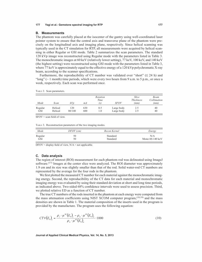
177 Yagi et al.: Gemstone spectral imaging for rTP 177
Journal of Applied Clinical Medical Physics, Vol. 14, no. 5, 2013
B. MeasurementsThe phantom was carefully placed at the isocenter of the gantry using well-coordinated laser pointer system to ensure that the central axis and transverse plane of the phantom were pre-cisely on the longitudinal axis and imaging plane, respectively. Since helical scanning was typically used in the CT simulation for RTP, all measurements were acquired by helical scan-ning in either Regular or GSI mode. Table 2 summarizes the scan parameters. The standard 120 kVp image was reconstructed using Regular mode with the parameters listed in Table 3. The monochromatic images at 60 keV (relatively lower setting), 77 keV, 100 keV, and 140 keV (the highest setting) were reconstructed using GSI mode with the parameters listed in Table 3, where 77 keV is approximately equal to the effective energy of a 120 kVp polychromatic X-ray beam, according to the scanner specifications.
Furthermore, the reproducibility of CT number was validated over “short” (≤ 24 h) and “long” (~ 1 month) time periods, which were every two hours from 9 a.m. to 5 p.m., or once a week, respectively. Each scan was performed once.
C. Data analysisThe region of interest (ROI) measurement for each phantom rod was delineated using ImageJ software.(17) Images at the center slice were analyzed. The ROI diameter was approximately 1.9 cm and its size was slightly smaller than that of the rod. Solid water-rod CT numbers are represented by the average for the four rods in the phantom.
We first plotted the measured CT number for each material against the monochromatic imag-ing energy. Second, the reproducibility of the CT data for each material and monochromatic imaging energy was evaluated by using their standard deviation at short and long time periods, as indicated above. Two-sided 68% confidence intervals were used to assess precision. Third, we plotted relative ED as a function of CT number.
The true CT numbers of the rods inserted in the phantom at each energy were computed from the mass attenuation coefficients using NIST XCOM computer program,(18,19) and the mass densities are shown in Table 1. The material composition of the inserts used in the program is provided by the manufacture. The program uses the following equation:
(10)
Table 2. Scan parameters.
Rotation Slice Beam Time Thickness Collimation Mode Scan kVp mA (s) SFOV (mm) (mm)
Regular Helical 120 630 0.5 Large body 2.5 40 GSI Helical 80/140 600 1.0 Large body 2.5 40
SFOV = scan field of view.
Table 3. Reconstruction parameters of the two imaging modes.
Mode DFOV (cm) Recon Kernel Energy
Regular 50 Standard N/A GSI 50 Standard Mono 60-140 keV
DFOV = display field of view, N/A = not applicable.

178 Yagi et al.: Gemstone spectral imaging for rTP 178
Journal of Applied Clinical Medical Physics, Vol. 14, no. 5, 2013
where ρj and μM(E0)j are the mass density of material j and mass attenuation coefficient of the material at energy E0, respectively. At room temperature, 0.99823 g/cm3 at 20°C was used as water mass density.
III. rESuLTS
A. Differences in CT number with different combinations of materials and monochromatic imaging energies
Figure 2 presents the CT images acquired by scanning in both modes. The 60 keV image con-tains an artifact appearing as a dark band around the cortical bone rod (Fig. 2(b), arrow). The magnitude of this artifact was reduced as monochromatic image energy increased. However,
Fig. 2. Overview of polychromatic and monochromatic images: a) 120 kVp, b) 60 keV, c) 77 keV, d) 100keV, e) 140 keV. The arrow indicates an artifact appearing as a dark band around the cortical bone rod.

179 Yagi et al.: Gemstone spectral imaging for rTP 179
Journal of Applied Clinical Medical Physics, Vol. 14, no. 5, 2013
a slight artifact around the rod was observed at 140 keV. The image at 100 keV was visibly better in quality in this study.
The CT number changed dramatically for high-density material rods as shown by the monochromatic images in Fig. 3. However, the CT number varied little in the materials with densities less than or equal to water, and CT number differences for high-energy images were less than those of lower energy images for the various material regions. The CT number range at 140 keV was about 1470 HU compared with 2300 HU at 60 keV, and was approximately 1.5-fold smaller at high energies.
Fig. 3. Distribution of CT number among materials as a function of monochromatic energy.
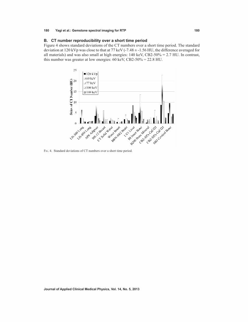
180 Yagi et al.: Gemstone spectral imaging for rTP 180
Journal of Applied Clinical Medical Physics, Vol. 14, no. 5, 2013
B. CT number reproducibility over a short time periodFigure 4 shows standard deviations of the CT numbers over a short time period. The standard deviation at 120 kVp was close to that at 77 keV (-7.48 ± -1.56 HU, the difference averaged for all materials) and was also small at high energies: 140 keV, CB2-50% = 2.7 HU. In contrast, this number was greater at low energies: 60 keV, CB2-50% = 22.8 HU.
Fig. 4. Standard deviations of CT numbers over a short time period.

181 Yagi et al.: Gemstone spectral imaging for rTP 181
Journal of Applied Clinical Medical Physics, Vol. 14, no. 5, 2013
C. CT number reproducibility over a long time periodFigure 5 shows standard deviations for CT numbers over a long time period. The trend was similar to that for a short time period, as stated above.
Fig. 5. Standard deviations of CT numbers over a long time period.

182 Yagi et al.: Gemstone spectral imaging for rTP 182
Journal of Applied Clinical Medical Physics, Vol. 14, no. 5, 2013
D. CT number differences between monochromatic image and theoretical valueThe CT number accuracy of the inserts was investigated. Figure 6 shows CT number differ-ence between monochromatic image and theoretical (true) value in soft tissues. As the energy increases, the difference is smaller. The 140 keV monochromatic image had the least amount of CT number deviation among the materials. Figure 7 shows differences between monochro-matic image and theoretical (true) CT number values in bony materials. The difference is less in images at higher energy. In SB3 cortical bone, the CT number is dramatically affected by the energy increases.
Fig. 6. CT number difference between monochromatic image (measured) and theoretical (true) value in soft tissues.
Fig. 7. CT number difference between monochromatic image (measured) and theoretical (true) value in bony materials.

183 Yagi et al.: Gemstone spectral imaging for rTP 183
Journal of Applied Clinical Medical Physics, Vol. 14, no. 5, 2013
E. CT number to ED conversion curves for monochromatic imagesFigure 8 shows the CT to ED conversion curves for various monochromatic images. These curves were generated from the short time period data. The curves plotted from the data for long time periods exhibited the similar trend and are, therefore, not presented here. The standard CT image curve displayed a bilinear relationship clustering around 0 HU (Fig. 8). There were no significant differences between the curves at numbers < water (0 HU). The curves’ shapes at 77 keV and 120 kVp were similar. The bilinear relationship gradually diminished with increas-ing energy. The curve for 140 keV was nearly linear.
IV. DISCuSSIon
Dual-energy CT provides clinically useful, material-specific information(9) in addition to the morphological information.(20,21) As a first step on the application of dual-energy CT for RTP, we evaluated the CT numbers of ED-known materials on monochromatic images obtained by the GSI operation mode.
In the GSI mode, the “monochromatic image” is reconstructed from “monochromatic projections”, which are calculated from 80 kVp and 140 kVp projections. In other words, the monochromatic image is not obtained with monochromatic X-ray projections, but “synthe-sized” with polychromatic 80 kVp and 140 kVp X-ray projections. It should be noted that the lowest energy (e.g., 60 keV) monochromatic image is predominantly derived from 80 kVp projections than 140 kVp ones. It is well known that lower energy X-rays are attenuated to a greater extent than higher energy X-rays when a polychromatic X-ray beam, especially one generated with a low tube voltage, passes through an object being imaged. This so-called beam hardening phenomenon(22) induces dark (or white) band artifacts because X-rays from some projection angles are hardened to a differing extent than rays from other angles. This confuses the reconstruction algorithm. The most common example occurs between the dense materials, and is demonstrated in Fig. 2(a) from 120 kVp imaging. This phenomenon could be theoretically suppressed with a “true” monochromatic X-ray, but remains in the “synthesized” monochromatic image, especially at a lower energy (Fig. 2(b)). Goodsitt et al.(23) also reported that the synthesized monochromatic images are not truly monochromatic, especially at lower energy. This is partly due to the scattering X-rays from outside the focal spot or surrounding material. The theory is not able to take into account the scatter effect while addressing the beam
Fig. 8. CT to ED conversion curves obtained by monochromatic images. The cutout shows the plots around 0 HU.

184 Yagi et al.: Gemstone spectral imaging for rTP 184
Journal of Applied Clinical Medical Physics, Vol. 14, no. 5, 2013
hardening effect. The scatter effect on dual-energy CT was studied by Vetter and Holden.(24) They found about 2% variations under different measurement conditions, and demonstrated nonlinearities in lookup tables due to the scatter effect. Their scanner had a collimator of 10 mm width. However, the GE scanner in this experiment used a 20 to 40 mm width. As a result, the scanner suffers from the scatter effect due to higher scatter fractions. In addition, the scatter fraction changes with each energy.(24) Implementing better scatter correction algorithms,(25) as well as increasing spectral separation between the low- and high-energy X-ray,(4,26,27) could improve the synthesized monochromatic image.
To our knowledge, there have been few reports using the GE scanner to study the CT number of various materials except for water.(23,28) The CT number changed dramatically for high-density materials in the different monochromatic images (Fig. 3). This result is consistent with data acquired using iodine solutions.(28) The high degree of change in CT numbers is caused by the dominance of the photoelectric effect over that of the Compton effect. The photoelectric effect probability at low energy is proportional to the atomic number cubed. In contrast, the Compton effect becomes dominant as the photon energy increases and is independent of atomic number. Therefore, the CT number varies little among diverse types of materials at high energy and explains why the CT number range is small for high-energy images.
CT number reproducibility during short and long time periods is quite important for any application using the CT number, such as the RTP system. To our knowledge, there are no reports of the stability over a day or a month. The stability of CT number of any materials is investigated only over the short term.(23,28) The trend of the CT number reproducibility was the same over a short or long time period, thus confirming the scanner stability. However, the standard deviation was somewhat large for CB2-50% at 60 keV. We consider that this might be due to the streak artifact reported by Papanikolaou et al.(29) This artifact would be, as described above, due to the fact that the image is not truly monochromatic. The artifact extended in a direction toward the CB2-50% rod (Fig. 2(b)). The artifact was reduced as the energy used to generate the monochromatic image was increased. This would explain the stability of CT number at the CB2-50% rod (Figs. 4 and 5). Although the large standard deviation may also result from noise on the 60 keV image, the noise is comparatively lower, as reported by Zhang et al.,(28) and would not primarily affect the standard deviation.
Image noise for given dose is also an important property. The noise determines the lower limit of subject contrast that can be distinguished by the observer. Less noise image would have more benefit for contouring objects, as well as dose calculation, in RTP. Theory predicts that there is an optimal energy for which the noise in the monochromatic energy has the same energy as in a regular CT, for the same given dose.(13) A study using a water-equivalent uniform phantom shows that the monochromatic images at the optimal energy have higher noise level than diagnostic X-ray energy range under the same acquisition and reconstruction conditions.(28) In our experiment (data not shown), in the monochromatic image the standard deviation within the ROI of the water insert showed a similar trend to previous studies — the noise dramatically decreases to the optimal energy and gradually increases as the energy increases.(13,28) The other inserts also showed a similar variation as the water insert. The noise of all inserts was also consistent over both short and long time periods. The noise is a very sensitive parameter to the overall imaging performance of the scanner. The scanner stability was also confirmed from this point of view.
An accurate dose calculation algorithm, as well as accurate determination of the relationship between CT number and ED, is required to accurately calculate dose distribution, minimiz-ing discrepancy between calculated and actual dose. Venselaar et al.(30) reported tolerances for the accuracy of RTP dose calculations. The accuracies required for dose calculations for homogeneous and heterogeneous media are 2% and 3%, respectively.(30) The 20 HU change in the CT number for soft tissues and 250 HU for bone result in about 1% of change for moni-tor unit (MU) for a brain case and 2% change for a lung and pelvis case.(29) The results could be transferred into the dose calculation in monochromatic image because the CT number is

185 Yagi et al.: Gemstone spectral imaging for rTP 185
Journal of Applied Clinical Medical Physics, Vol. 14, no. 5, 2013
normalized to water. In our experiment, the results show such changes in monochromatic images at lower energy (e.g., 60 keV) between measured and true value in several tissues, but not in bony materials (Figs. 6 and 7). CT number stability results also compensate the accu-racy. The study, however, shows larger difference below 60 keV in soft tissue and bone than the criteria described above (i.e., 20 HU for soft tissue and 250 HU for bone).(23) That implies that the dose calculation on monochromatic images lower than 60 keV would result in larger dosimetric differences compared with other energies. The other important factor for the dose calculation is the phantom (body) size because size changes the X-ray attenuation, as well as the amount of scatter from surrounding material, resulting in CT number change. The size has a high impact on CT number.(31) Bone CT numbers under several composition variations considerably differ between small and large phantom size on monochromatic image at each energy.(23) A phantom of proper size, which is close to a subsequently irradiated part such as head or body, should be scanned.
The CT to ED conversion curves with monochromatic images were determined for RTP. A linear relationship was observed at 140 keV, while the curves in the low-energy image were bilinear, bordering around 0 HU (Fig. 8). At high energies, the Compton effect is dominant over the photoelectric effect, similar to that of megavoltage cone beam CT (MVCBCT).(32) However, the dose calculation for MVCBCT has proven not to be practical because of problems, such as cupping artifacts.(33) Reflecting the Compton effect compared with standard CT images used clinically for CT simulation would predict that dose calculation is performed more accurately using high-energy monochromatic images without the problems associated with MVCBCT.(33) Dosimetric investigation is required for the further evaluation of the dose calculation accuracy with these CT to ED conversion curves.
V. ConCLuSIonS
This is the first report regarding the CT to ED conversion curves for RTP by a CT scanner with a fast kVp switching system. We present here CT to ED conversion curves acquired from monochromatic images for RTP, assessing CT number accuracy. Reproducibility was confirmed by determining the variation in CT number.
ACknowLEDGMEnTS
This work was supported by a Grant-in-Aid for Scientific Research (no. 21611004) from the Ministry of Education, Culture, Sports, Science and Technology, Japan grants.
rEFErEnCES
1. Aird E, Conway J. CT simulation for radiotherapy treatment planning. Br J Radiol. 2002;75(900):937–49. 2. Hounsfield GN. Computerized transverse axial scanning (tomography): Part 1. Description of system. Br J Radiol.
1973;46(552):1016–22. 3. Rutherford RA, Pullan BR, Isherwood I. Measurement of effective atomic number and electron density using an
EMI scanner. Neuroradiology. 1976;11(1):15–21. 4. Rutherford RA, Pullan BR, Isherwood I. X-ray energies for effective atomic number determination. Neuroradiology.
1976;11(1):23–28. 5. Brooks RA. A quantitative theory of the Hounsfield unit and its application to dual energy scanning. J Comput
Assist Tomogr. 1977;1(4):487–93. 6. Alvarez RE and Macovski A. Energy-selective reconstructions in X-ray computerized tomography. Phys Med
Biol. 1976;21(5):733–44. 7. Kalender WA, Perman W, Vetter J, Klotz E. Evaluation of a prototype dual-energy computed tomographic appa-
ratus. I. Phantom studies. Med Phys. 1986;13(3):334–39.

186 Yagi et al.: Gemstone spectral imaging for rTP 186
Journal of Applied Clinical Medical Physics, Vol. 14, no. 5, 2013
8. Maass C, Baer M, Kachelriess M. Image-based dual energy CT using optimized precorrection functions: a practi-cal new approach of material decomposition in image domain. Med Phys. 2009;36(8):3818–29.
9. Santamarıa-Panga A, Duttab S, Makrogiannisc S, et al. Automated liver lesion characterization using fast kVp switching dual energy computed tomography imaging. In: Karssemeijer N and Summers RM, editors. Medical Imaging 2010: Computer Aided Diagnosis. Proc of SPIE 2010;7624.
10. Vetter J, Perman W, Kalender WA, Mazess R, Holden J. Evaluation of a prototype dual-energy computed tomo-graphic apparatus. II. Determination of vertebral bone mineral content. Med Phys. 1986;13(3):340–43.
11. Montner SM, Lehr JL, Oravez WT. Quantitative evaluation of a dual energy CT system. J Comput Assist Tomogr. 1987;11(1):144–50.
12. Lehmann L, Alvarez R, Macovski A, et al. Generalized image combinations in dual KVP digital radiography. Med Phys. 1981;8(5):659–67.
13. Alvarez R, Seppi E. A comparison of noise and dose in conventional and energy selective computed tomography. Nuclear Science, IEEE Transactions on. 1979;26(2):2853–56.
14. Storm E and Israel HI. Photon cross sections from 1 keV to 100 MeV for elements Z = 1 to Z = 100. Los Alamos, NM: Los Alamos Scientific Laboratory; 1970.
15. Slaney M and Kak A. Principles of computerized tomographic imaging. Philadelphia, PA: SIAM; 1988. 16. Gammex Inc. Tissue characterization phantom Gammex 467 user’s guide [cited 2012 12/20]. Available from:
http://www.gammex.com/n-portfolio/productpage.asp?id=283&category=Radiation+Oncology&name=Tissue+Characterization+Phantom%2C+Gammex+467
17. Abràmoff MD, Magalhães PJ, Ram SJ. Image processing with ImageJ. Biophotonics International. 2004;11(7):36–42.
18. Berger M, Hubbell J, Seltzer S, et al. XCOM: photon cross sections database, NIST standard reference database 8 (XGAM). 2005. Available from: http://www.nist.gov/pml/data/xcom/index.cfm
19. Hubbell JH. Photon cross sections, attenuation coefficients, and energy absorption coefficients from 10 keV to 100 GeV. NSRDS–NBS29. Washington, DC: NIST; 1969.
20. Neville AM, Gupta RT, Miller CM, Merkle EM, Paulson EK, Boll DT. Detection of renal lesion enhancement with dual-energy multidetector CT. Radiology. 2011;259(1):173–83.
21. Lv PJ, Lin XZ, Li JY, Li WX, Chen KM. Differentiation of small hepatic hemangioma from small hepatocellular carcinoma: recently introduced spectral CT method. Radiology. 2011;259(3):720–29.
22. Bushberg JT, Seibert JA, Leidholdt EM, Boone JM. The essential physics of medical imaging. Philadelphia, PA: Lippincott Williams & Wilkins; 2001.
23. Goodsitt MM, Christodoulou EG, Larson SC. Accuracies of the synthesized monochromatic CT numbers and effective atomic numbers obtained with a rapid kVp switching dual energy CT scanner. Med Phys. 2011;38(4):2222–32.
24. Vetter J and Holden J. Correction for scattered radiation and other background signals in dual-energy computed tomography material thickness measurements. Med Phys. 1988;15(5):726–31.
25. Cardinal HN and Fenster A. An accurate method for direct dual-energy calibration and decomposition. Med Phys. 1990;17(3):327–41.
26. Primak A, Ramirez Giraldo JC, Liu X, Yu L, McCollough C. Improved dual-energy material discrimination for dual-source CT by means of additional spectral filtration. Med Phys. 2009;36(4):1359–69.
27. Yang M, Virshup G, Clayton J, Zhu X, Mohan R, Dong L. Does kV–MV dual-energy computed tomography have an advantage in determining proton stopping power ratios in patients? Phys Med Biol. 2011;56(14):4499–515.
28. Zhang D, Li XH, Liu B. Objective characterization of GE Discovery CT750 HD scanner: gemstone spectral imaging mode. Med Phys. 2011;38(3):1178–88.
29. Papanikolaou N, Battista J, Boyer A, et al. Tissue inhomogeneity corrections for megavoltage photon beams. AAPM Task Group 65. Madison (WI): Medical Physics Publishing; 2004.
30. Venselaar J, Welleweerd H, Mijnheer B. Tolerances for the accuracy of photon beam dose calculations of treat-ment planning systems. Radiother Oncol. 2001;60(2):191–201.
31. Joseph PM and Spital RD. The effects of scatter in x-ray computed tomography. Med Phys. 1982;9(4):464–72. 32. Petit SF, van Elmpt WJC, Nijsten SM, Lambin P, Dekker AL. Calibration of megavoltage cone-beam CT for
radiotherapy dose calculations: correction of cupping artifacts and conversion of CT numbers to electron density. Med Phys. 2008;35(3):849–65.
33. Morin O, Chen J, Aubin M, et al. Dose calculation using megavoltage cone-beam CT. Int J Radiat Oncol Biol Phys. 2007;67(4):1201–10.

a Corresponding author: Gitte Fredberg Persson, Department of Oncology 5073, Rigshospitalet, Blegdamsvej 7-9, 2100 Copenhagen, Denmark; phone: +45 3545 9775; fax: +45 35453990; email: [email protected]
Stability of percutaneously implanted markers for lung stereotactic radiotherapy
Gitte F. Persson,1,2a Mirjana Josipovic,1 Peter von der Recke,1,3 Marianne C. Aznar,1,4 Trine Juhler-Nøttrup,5 Per Munck af Rosenschöld,1,4 Stine Korreman,1,4,6 and Lena Specht1,2,7
Department of Radiation Oncology,1 Copenhagen University Hospital, Rigshospitalet, Copenhagen, Denmark; Department of Oncology,2 Copenhagen University Hospital, Rigshospitalet, Copenhagen, Denmark; Department of Radiology,3 Copenhagen University Hospital, Rigshospitalet, Copenhagen, Denmark; Faculty of Science,4 Niels Bohr Institute, University of Copenhagen, Copenhagen, Denmark; Department of Oncology,5 Copenhagen University Hospital, Herlev Hospital, Herlev, Denmark; Department of Science,6 Systems and Models, Roskilde University, Roskilde, Denmark; Faculty of Medical Sciences,7 University of Copenhagen, Copenhagen, [email protected]
Received 1 January, 2013; accepted 25 April, 2013
The purpose of this study was to evaluate the stability of complex markers implanted into lung tumors throughout a course of stereotactic body radiotherapy (SBRT). Fifteen patients referred for lung SBRT were prospectively included. Radio-opaque markers were implanted percutaneously, guided by computed tomography (CT). Deep inspiration breath-hold CT scans (BHCT) were acquired at planning and on three treatment days. The treatment days’ BHCTs were registered to the planning BHCT. Intraobserver uncertainty in both tumor and marker registration was determined. Deviations in the difference between tumor and marker-based image registrations of the BHCT scans during treatment quantified the marker stability. Marker position deviation relative to tumor position of less than 2 mm in all three dimensions was considered acceptable for treatment delivery precision. Intra-observer uncertainties for image registration in the left–right (LR), anterior–posterior (AP), craniocaudal (CC) directions and three-dimensional vector (3D) were 0.9 mm, 0.9 mm, 1.0 mm, and 1.1 mm (SD) for tumor registration and 0.3 mm, 0.5 mm, 0.7 mm, and 0.7 mm (SD) for marker registration. Mean 3D differences for tumor registrations on all days were significantly larger than for 3D marker registrations (p = 0.007). Overall median differences between tumor and marker position were 0.0 mm (range -2.9 to 2.6 mm) in LR, 0.0 mm (-1.8 to 1.5 mm) in AP, and -0.2 mm (-2.6 to 2.8 mm) in CC directions. Four patients had deviations exceeding 2 mm in one or more registrations throughout the SBRT course. This is the first study to evaluate stability of complex markers implanted percutaneously into lung tumors for image guidance in SBRT. We conclude that the observed stability of marker position within the tumor indicates that complex markers can be used as surrogates for tumor position during a short course of SBRT as long as the uncertainties related to their position within the tumor are incorporated into the planning target volume.
PACS number: 87.57.nj, 87.55.ne
Key words: fiducial markers, lung tumors, image-guidance, stability, stereotactic body radiotherapy
JOURNAL OF APPLIED CLINICAL MEDICAL PHYSICS, VOLUME 14, NUMBER 5, 2013
187 187

188 Persson et al.: Stability of implanted markers for SBRT 188
Journal of Applied Clinical Medical Physics, Vol. 14, No. 5, 2013
I. INTRODUCTION
Lung tumors move during breathing, and tumor motion of more than 3 cm has been seen for tumors located near the diaphragmatic domes.(1) Breathing-adapted radiotherapy, such as respira-tory beam gating or tumor tracking, compensates for tumor motion by only irradiating during a prespecified part of the breathing cycle or by letting the treatment beam follow the tumor motion. Both approaches rely on the ability to determine and predict the breathing-related tumor motion based on an external or internal surrogate for tumor motion. The prediction of the correlation between the tumor and the surrogate positions must be verified throughout the treatment; the verification can be performed with repeated kV imaging of the tumor. However, not all lung tumors are well defined on kV images and, therefore, radio-opaque markers implanted in or close to the tumor have been used as a surrogate for tumor position. Markers can be implanted percutaneously, guided by fluoroscopy or computed tomography (CT), or transbronchially, inserted in nearby small bronchi. The advantage of percutaneous implantation is the possibility to implant the marker directly into the tumor, assuring a good representation of tumor motion, but potentially at the cost of morbidity due to the risk of pneumothorax. Bronchoscopic inser-tion implies less morbidity, but insertion directly into the tumor is difficult and the stability of the markers has been questioned.(2,3)
When the position of the radio-opaque markers is used as surrogate for tumor position dur-ing radiotherapy, it is important that the position of the markers relative to the tumor is stable throughout the course of radiotherapy. The stability of markers implanted for long-course fractionated radiotherapy has previously been evaluated,(4) but this is not the case for short-course SBRT.
The aim of this study was to evaluate the stability of the position of complex radio-opaque mark-ers relative to the lung tumor throughout a course of stereotactic body radiotherapy (SBRT).
II. MATERIALS AND METHODS
Fifteen patients were prospectively included between February 2009 and December 2010. Data collection was approved by the Danish Data Protection Agency (j.nr. 30-0484). The study was approved by the local ethical committee (jr.nr. H-B-2007-016) and reported to Clinicaltrials.gov (ClinicalTrials.gov Identifier: NCT00910546).
Study inclusion criteria were: referral for SBRT, non-small cell lung cancer (NSCLC) or lung metastases, age > 40 years, WHO performance status < 2, and obtained signed informed consent. Exclusion criteria were: forced expiratory volume in 1 second (FEV1) > 0.5 l, centrally located tumor, or tumor located close to large vessels.
All marker implantations were performed CT-guided by the same radiologist, one week prior to treatment planning and two weeks prior to treatment start. Markers were changed during the study. The first five patients had implanted a Visicoil (IBA Dosimetry, Bartlett, TN) gold marker measuring 0.75 mm × 2 cm. Patient no. 6 had implanted a complex helical platinum coil (Boston Scientific, Natick, MA) measuring 20 mm restrained and 2 × 4 × 4 mm unrestrained. Patients 7 to 15 had implanted a Gold Anchor marker (Naslund Medical, Huddinge, Sweden) measuring 0.28 × 20 mm. For all patients only a single marker was implanted. All markers were complex in structure (Fig. 1).
The planning protocol for SBRT consisted of a PET/CT with contrast enhancement and, within two subsequent days, a 4D CT and a voluntary deep inspiration breath-hold CT (BHCT) in the same session. Treatment planning was performed on the midventilation phase of the 4D CT, and a total dose of 45 Gy was delivered in 3 fractions within five to eight days. On all three treatment days a BHCT was acquired.
The BHCT scans were acquired during deep inspiration breath-hold (10–20 seconds) without contrast enhancement, on a Siemens Sensation Open multislice CT scanner (Siemens Healthcare,

189 Persson et al.: Stability of implanted markers for SBRT 189
Journal of Applied Clinical Medical Physics, Vol. 14, No. 5, 2013
Erlangen, Germany) in a helical scan mode with a pitch of 1.2 and reconstructed with a pixel size of 0.98 mm × 0.98 mm and 3 mm plane separation.
For the purpose of the BHCT, the patient was asked to take a deep inspiration and hold it during the scan. The respiration signal was monitored with the Real-time Position Management (RPM) system (Varian Medical Systems, Palo Alto, CA).
The BHCT scans were used for evaluation of marker stability, rather than the 4D CT, to avoid potential motion artifacts.(5) To evaluate the stability of the marker’s position, the planning BHCT (CT0) was rigidly registered to the BHCT scans of the three treatment days (CT1-3) by a single observer. Both tumor and marker registrations were performed. A window setting of 700 Hounsfield units (HUs) with a level of -300 HU was used. Only translations were used for the image registration, since rotations can be difficult to assess with small spherical tumors. The difference between tumor and marker registration was used as a measure of the stability of the marker position within the tumor and was evaluated for the translational directions: left–right (LR), anterior–posterior (AP), and craniocaudal (CC). Furthermore, 3D vector displacement was calculated. A difference in marker position within the tumor of less than 2 mm in one of the three translational directions was considered acceptable for treatment precision.
To evaluate the extent of intra-observer variation all the rigid registrations were performed twice. The standard deviation (SD) of the differences between the two registrations of the tumor was a measure of the intra-observer variation in tumor registration, and the SD of the differences between the two registrations of the marker was a measure of the intra-observer variation in marker registration.
The evaluation of the marker position deviation within the tumor was evaluated for all four combinations of differences between the tumor and the marker registration (i.e., the first tumor registration vs. the first and second marker registration, respectively, and the second tumor registration vs. the first and second marker registration, respectively). The mean of the four values was used in the analysis of the marker stability.
Parametric statistics with calculation of SD were applied for intra-observer variation data as these were considered Gaussian-distributed. The data concerning the stability were considered to be influenced by both the intra-observer variation and the position deviation of the marker relative to the tumor, and therefore nonparametric statistics were applied.
Fig. 1. Photo showing the complex helical platinum marker (top), the Gold Anchor marker (middle), and the Visicoil gold marker (bottom).

190 Persson et al.: Stability of implanted markers for SBRT 190
Journal of Applied Clinical Medical Physics, Vol. 14, No. 5, 2013
III. RESULTS
Patient characteristics are presented in Table 1. Only 14 patients were eligible for the stability evaluation. The marker of patient no. 2 disappeared between the planning scan and the treatment start. It had been placed in proximity to a bronchus and the patient had been reported coughing. It is hypothesized that the marker was coughed up, as a full-body CT revealed no sign of the marker. Patient no. 8 was excluded after the first treatment session as the performance status had deteriorated and the treatment was terminated. For patients no. 5 and 15, scans from the second treatment sessions were missing because of technical issues. Altogether, data acquisi-tions were incomplete for four out of the 15 patients. In patient no. 6, the only patient with the complex helical platinum coil, the marker was implanted 1 cm below the tumor.
Intra-observer variations in tumor registrations were 0.9 mm in LR, 0.9 mm in AP, 1.0 mm in CC direction, and 1.2 mm in 3D. Mean absolute deviations were 0.5 mm in LR, 0.6 mm in AP, 0.7 mm in CC direction, and 1.2 mm in 3D. For three patients (no. 3, 10, and 13), tumor match deviations exceeded 2 mm for one or two matches in one or two directions.
Intra-observer variations marker registrations were 0.3 mm in LR, 0.5 mm in AP, 0.7 mm in CC direction, and 0.7 mm in 3D. Mean absolute deviations were 0.2 mm in LR, 0.3 mm in AP, 0.5 mm in CC, and 0.7 mm in 3D. No deviations in marker match exceeded 2 mm.
Intra-observer variation for tumor registration was significantly larger than for marker reg-istration (p = 0.007, paired Student’s t-test).
Overall median differences between tumor and marker position were 0.0 mm (range -2.9 to 2.6 mm) in LR, 0.0 mm (-1.8 to 1.5 mm) in AP, and -0.2 mm (-2.6 to 2.8 mm) in CC direc-tions. The median absolute values for differences between tumor and marker positions were 0.3 mm (range 0–2.9 mm) in LR, 0.4 mm (0.1–1.8 mm) in AP, and 0.9 mm (0.1–2.8 mm) in CC directions. Median difference between tumor and marker position in 3D was 1.3 mm (range 0.4 to 4.3 mm).
Two patients (no. 1 and 14) had one single deviation between tumor and marker position exceeding 2 mm, both in the CC direction. Two patients (no. 3 and 13) had deviations in two or more registrations exceeding 2 mm; patient no. 13 had consistent deviations between tumor and marker position of 2.1 to 2.9 mm in the LR direction indicating a displacement of the marker between planning and treatment. Deviations for all patients are shown in Fig. 2.
Table 1. Patient characteristics.
Agea 73 (60–87) yearsGender Female / Male 7 / 8FEV1a 1.4 (0.7–3.4) L
Diagnosis NSCLC 14 Lung metastases 1
Tumor Location Upper lobe 6 Lower lobe 9
Tumor Size Diametera 3.6 (1.5–7.0) cm Volumea 13.6 (1.7–46.3) cm3
Left–Right 0.2 (0.1–0.3) cmTumor Motiona Antero–Posterior 0.2 (0.1–0.4) cm Craniocaudal 0.6 (0.1–2.4) cm
a Median (range)

191 Persson et al.: Stability of implanted markers for SBRT 191
Journal of Applied Clinical Medical Physics, Vol. 14, No. 5, 2013
Fig. 2. Position deviation of the marker relative to the tumor for all patients (BHCT0 as reference) at the first (■), the second (■), and the third (■) treatment day.

192 Persson et al.: Stability of implanted markers for SBRT 192
Journal of Applied Clinical Medical Physics, Vol. 14, No. 5, 2013
IV. DISCUSSION
For nine of the evaluated 13 patients, all deviations between tumor and marker position were within 2 mm. For two of the remaining four patients only one measured marker position devia-tion exceeded the 2 mm threshold. The median (and the mean) deviations in all translational directions were close to zero, indicating a random uncertainty.
The analysis of intra-observer variation was performed to have an order of magnitude for the general uncertainty of the registration procedure for marker and tumor registration. The intra-observer variation of the tumor match was 0.9 to 1.0 mm (SD), depending on direction. Most of the observed differences between tumor and marker position were within the intra-observer uncertainty for tumor registration.
Two patients (no. 3 and 13) had larger deviations in marker position. This observed varia-tion was probably caused by poorly defined tumors which were difficult to match, as the intra-observer variations in tumor match were largest for the same two patients. In patient no. 13, the tumor had poorly defined edges and was located close to the diaphragm, which resulted in 3 cm peak-to-peak motion in CC direction during free breathing. In patient no. 3, the tumor was embedded in fibrous tissue caused by earlier breast cancer irradiation. The marker was implanted in the periphery of the tumor, which may also have had an impact on the registration results. Smith et al.(6) found that the closer to the tumor center the marker was implanted, the better it followed the tumor position, since tumor tissue is more rigid than surrounding lung parenchyma, while correlation between tumor motion and marker motion deteriorates as the distance from the marker to the tumor increases. Patient no. 6 had the marker implanted 1 cm inferior to the tumor; nevertheless, the marker stability in this patient did not stand out (see Fig. 2), possibly because the tumor was located in the lung apex where tumor and lung tissue motion is minimal. In our study, one of the patients presumably coughed up the marker. This problem is more often encountered with markers implanted by bronchoscope,(2,7,8,9) and can be seen as an extreme deviation of marker position. This patient was excluded from the analysis, thus biasing the study. In a clinical setting using a marker-based image-guidance protocol, the patient would have had the marker replaced.
Intra-observer variation of tumor registration was approximately twice the intra-observer variation of marker registration. This difference was due to high radio-opacity of the markers in the CT compared to the tumor, in addition to a well-defined shape. Visicoil marker resulted in a higher degree of metal streaking artifacts in the CT images than the complex platinum coil and the Gold Anchor; however, these artifacts did not impact the visual definition of the marker shape. Lack of rotations in registration may also have affected the intra-observer variation. Josipovic et al.(10) showed that omitting rotational position corrections when applying soft tissue tumor registration as image guidance in SBRT, a systematic error of 1 mm (SD) was introduced
By visual evaluation of the thoracic orthogonal kV X-rays acquired four hours after the marker implantation (Fig. 3), it was clear that the Visicoil marker provided the highest radio-opacity. The two other markers provided equal radio-opacity. However, the radio-opacity of the Gold Anchor marker depended on the intratumoral folding of the marker.
Kupelian et al.(4) included 15 patients for percutaneous implantation of Visicoil markers and eight patients for transbronchial implantation of metallic fiducial markers in lung tumors. The majority of the patients received long-course radiotherapy (70 Gy / 35 fractions). Expiration breath-hold CT scans were acquired at planning and at a point during treatment or at follow-up. The two scans were compared and the marker position deviation was estimated. For all patients, no translational deviations in marker position relative to the tumor larger than 5 mm were seen. As pointed out by the authors, tumor shrinkage of 34% ± 23% throughout the observation period impacted the results. The latter probably also explains that the reported deviations were significantly larger than in the present study with a much shorter treatment and observation time.

193 Persson et al.: Stability of implanted markers for SBRT 193
Journal of Applied Clinical Medical Physics, Vol. 14, No. 5, 2013
Roman et al.(11) analyzed weekly 4D CT scans of seven patients with locally advanced NSCLC and bronchoscopically implanted gold coils receiving long-course radiotherapy. They found interfractional marker-to-tumor centroid displacements of 2–3 mm both systematically and randomly in the three translational directions. They also found significant change in the displacements over time.
Van den Vort van Zyp et al.(12) examined the stability of 111 smooth platinum markers implanted percutaneously in 44 lesions of 42 patients with lung tumors. BHCT were performed two or three times during a hypofractionated treatment course. They found a median marker displacement of 1.2 mm, but 12% of the markers moved more than 5 mm and 5% of the markers moved more than 10 mm. This displacement was also larger than the displacement found in our study and could be caused by the smooth structure of the markers compared to the complex or coiled structure of the markers in our study.
Schroeder et al.(8) reported that coils are more stable than linear markers. Studies(2,3,9) using spherical, cylindrical or linear markers reported marker migration rates of 10% to 69%, which was taken into account by the insertion of multiple markers. Also Hong et al.,(13) in a retrospec-tive study including 54 consecutive patients, found that coil markers were better retained than seed markers. In several other studies,(2,3,7,8,9,14,15,16,17,18,19) multiple markers per tumor were implanted, as well. A single marker was implanted only in cases of small tumors, such as in our study. The advantage of multiple implanted markers is the possibility of using pattern recogni-tion to check for tumor rotation, deformation, and displacements of markers during treatment. However, use of multiple markers also increases the risk of pneumothorax, compared to using a single marker.(12,15)
A limitation of the present study is the limited number of patients included. However, a rigid imaging and data processing protocol enhances the validity of the study.
Use of different marker types in our study represented an unscheduled modification of the clinical protocol. The marker types were changed during the study by request of the radiologist.
Fig. 3. Chest X-rays showing different marker types. Patient 1 had a 2 cm long helical gold marker (Visicoil) implanted in the tumor in the right inferior lung lobe (left). Patient 6 had the complex helical platinum marker (Boston Scientific) implanted in the tumor in right superior lung lobe (middle). Note that the marker was placed outside the tumor. The patient had a pacemaker. Patient 11 had the Gold Anchor marker implanted in the tumor in the right inferior lobe (right). The arrows indicate the position of the markers.

194 Persson et al.: Stability of implanted markers for SBRT 194
Journal of Applied Clinical Medical Physics, Vol. 14, No. 5, 2013
The gold Visicoil marker gave the best radio-opacity in kV imaging, but the implantation needle’s outer diameter was 1.27 mm and resulted in two cases (patients no. 4 and 5) of pneu-mothorax; therefore, the marker was changed to the Boston Scientific complex helical coil (Boston Scientific, Natick, MA) for patient no. 6. However, this marker was not preloaded into the implantation needle and the instrumentation was difficult. The Gold Anchor marker was preloaded and inserted through a thinner needle (outer diameter 0.53 mm) minimizing the risk of pneumothorax, although two of the nine patients implanted with this marker had a pneumothorax (patients no. 7 and 10). The thin needle however, was very flexible, making its steering challenging. In our opinion, the optimal marker for IGRT and insertion method is yet to be found.
In our study, as in other studies examining marker stability,(2,12,16,19,20) CT scans were used for the evaluation. It is important to be aware that interpolations in CT imaging will inherently lead to intramodality uncertainty in imaging, hence compromising the precision of information in images. In a recent study by Oxnard et al.,(21) the variability between tumor size measure-ments on repeated BHCT showed differences exceeding 2 mm for a third of the patients.
V. CONCLUSIONS
Overall we conclude that the deviations of marker position in the tumor were within the mag-nitude of the intra-observer variation of the registration procedure for the majority of patients, and that the intra-observer uncertainty in marker registration was significantly smaller than in tumor registration. The observed stability of marker position within the tumor indicates that markers implanted in lung tumors can be used as surrogates for tumor position during a short course of SBRT as long as the uncertainties related to their position within the tumor are incorporated into the planning target volume.
ACkNOwLEDgMENTS
The authors have received grants from The Danish Council for independent Research in Medical Sciences”, The Arvid Nilssons Foundation, and The Astrid Thaysens Foundation.
REFERENCES
1. Keall PJ, Mageras GS, Balter JM, et al. The management of respiratory motion in radiation oncology report of AAPM Task Group 76. Med Phys. 2006;33(10):3874–900.
2. Nelson C, Starkschall G, Balter P, Morice RC, Stevens CW, Chang JY. Assessment of lung tumor motion and setup uncertainties using implanted fiducials. Int J Radiat Oncol Biol Phys. 2007;67(3):915–23.
3. Harley DP, Krimsky WS, Sarkar S, Highfield D, Aygun C, Gurses B. Fiducial marker placement using endobron-chial ultrasound and navigational bronchoscopy for stereotactic radiosurgery: an alternative strategy. Ann Thorac Surg. 2010;89(2):368–73.
4. Kupelian PA, Forbes A, Willoughby TR, et al. Implantation and stability of metallic fiducials within pulmonary lesions. Int J Radiat Oncol Biol Phys. 2007;69(3):777–85.
5. Persson GF, Nygaard DE, Munck af Rosenschöld PM. et al. Artifacts in conventional computed tomography (CT) and free breathing four-dimensional CT induce uncertainty in gross tumor volume determination. Int J Radiat Oncol Biol Phys. 2011;80(5):1573–80.
6. Smith RL, Yang D, Lee A, Mayse ML, Low DA, Parikh PJ. The correlation of tissue motion within the lung: implications on fiducial based treatments. Med Phys. 2011;38(11):5992–97.
7. Shirato H, Harada T, Harabayashi T, et al. Feasibility of insertion/implantation of 2.0-mm-diameter gold internal fiducial markers for precise setup and real-time tumor tracking in radiotherapy. Int J Radiat Oncol Biol Phys. 2003;56(1):240–47.
8. Schroeder C, Hejal R, Linden PA. Coil spring fiducial markers placed safely using navigation bronchoscopy in inoperable patients allows accurate delivery of CyberKnife stereotactic radiosurgery. J Thorac Cardiovasc Surg. 2010;140(5):1137–42.

195 Persson et al.: Stability of implanted markers for SBRT 195
Journal of Applied Clinical Medical Physics, Vol. 14, No. 5, 2013
9. Imura M, Yamazaki K, Shirato H, et al. Insertion and fixation of fiducial markers for setup and tracking of lung tumors in radiotherapy. Int J Radiat Oncol Biol Phys. 2005;63(5):1442–47.
10. Josipovic M, Persson GF, Logadottir A, Smulders B, Westmann G, Bangsgaard JP. Translational and rotational intra- and inter-fractional errors in patient and target position during a short course of frameless stereotactic body radiotherapy. Acta Oncol. 2012;51(5):610–17.
11. Roman NO, Shepard W, Mukhopadhyay N, Hugo GD, Weiss E. Interfractional positional variability of fiducial markers and primary tumors in locally advanced non-small-cell lung cancer during audiovisual biofeedback radiotherapy. Int J Radiat Oncol Biol Phys. 2012;83(5):1566–72.
12. van der Voort van Zyp N, Hoogeman MS, van de Water S, et al. Stability of Markers Used for Real-Time Tumor Tracking After Percutaneous Intrapulmonary Placement. Int J Radiat Oncol Biol Phys. 2011;81(3):e75–e81.
13. Hong JC, Yu Y, Rao AK, et al. High retention and safety of percutaneously implanted endovascular embolization coils as fiducial markers for image-guided stereotactic ablative radiotherapy of pulmonary tumors. Int J Radiat Oncol Biol Phys. 2011;81(1):85–90.
14. Pennathur A, Luketich JD, Heron DE, et al. Stereotactic radiosurgery for the treatment of lung neoplasm: experi-ence in 100 consecutive patients. Ann Thorac Surg. 2009;88(5):1594–600.
15. Nuyttens JJ, Prevost JB, Praag J, et al. Lung tumor tracking during stereotactic radiotherapy treatment with the CyberKnife: marker placement and early results. Acta Oncol. 2006;45(7):961–65.
16. Kothary N, Heit JJ, Louie JD, et al. Safety and efficacy of percutaneous fiducial marker implantation for image-guided radiation therapy. J Vasc Interv Radiol. 2009;20(2):235–39.
17. Collins BT, Erickson K, Reichner CA, et al. Radical stereotactic radiosurgery with real-time tumor motion tracking in the treatment of small peripheral lung tumors. Radiat Oncol. 2007;2:39.
18. Collins BT, Vahdat S, Erickson K, et al. Radical cyberknife radiosurgery with tumor tracking: an effective treatment for inoperable small peripheral stage I non-small cell lung cancer. J Hematol Oncol. 2009;2:1.
19. Bhagat N, Fidelman N, Durack JC, et al. Complications associated with the percutaneous insertion of fiducial markers in the thorax. Cardiovasc Intervent Radiol. 2010;33(6):1186–91.
20. Sotiropoulou E, Stathochristopoulou I, Stathopoulos K, Verigos K, Salvaras N, Thanos L. CT-guided fidu-cial placement for cyberknife stereotactic radiosurgery: an initial experience. Cardiovasc Intervent Radiol. 2010;33(3):586–89.
21. Oxnard GR, Zhao B, Sima CS, et al. Variability of lung tumor measurements on repeat computed tomography scans taken within 15 minutes. J Clin Oncol. 2011;29(23):3114–19.
a Corresponding author: Nakorn Phaisangittisakul, Department of Physics, Faculty of Science, Chulalongkorn University, Payatai Road, Patumwan, Bangkok 10330 Thailand; phone: (662) 218-7542; fax: (662) 253-1150; email: [email protected]
Equivalent square formula for determining the surface dose of rectangular field from 6 MV therapeutic photon beam
Lukkana Apipunyasopon,1 Somyot Srisatit,1 Nakorn Phaisangittisakul2,3a
Department of Nuclear Engineering,1 Faculty of Engineering, Chulalongkorn University, Bangkok, Thailand; Department of Physics,2 Faculty of Science, Chulalongkorn University, Bangkok, Thailand; ThEP Center,3 CHE, 328 Si-Ayuttaya Road, Bangkok, [email protected]
Received 2 January, 2013; accepted 8 April, 2013
The purpose of the study was to investigate the use of the equivalent square for-mula for determining the surface dose from a rectangular photon beam. A 6 MV therapeutic photon beam delivered from a Varian Clinac 23EX medical linear accelerator was modeled using the EGS4nrc Monte Carlo simulation package. It was then used to calculate the dose in the build-up region from both square and rectangular fields. The field patterns were defined by various settings of the X- and Y-collimator jaw ranging from 5 to 20 cm. Dose measurements were performed using a thermoluminescence dosimeter and a Markus parallel-plate ionization cham-ber on the four square fields (5 × 5, 10 × 10, 15 × 15, and 20 × 20 cm2). The surface dose was acquired by extrapolating the build-up doses to the surface. An equivalent square for a rectangular field was determined using the area-to-perimeter formula, and the surface dose of the equivalent square was estimated using the square-field data. The surface dose of square field increased linearly from approximately 10% to 28% as the side of the square field increased from 5 to 20 cm. The influence of collimator exchange on the surface dose was found to be not significant. The difference in the percentage surface dose of the rectangular field compared to that of the relevant equivalent square was insignificant and can be clinically neglected. The use of the area-to-perimeter formula for an equivalent square field can provide a clinically acceptable surface dose estimation for a rectangular field from a 6 MV therapy photon beam.
PACS number: 87.55.ne
Key words: surface dose, build-up dose, rectangular field, equivalent square, Monte Carlo simulation
I. IntroductIon
High-energy photons generated by a medical linear accelerator have been commonly used in radiotherapy. With an increasing energy of ionizing radiation, the penetrating power of photons and secondary electrons increases, leading to a deeper position of the point of maximum dose. However, the accumulated dose at the boundary between the air and patient’s skin, which is known as the surface dose, is not clinically negligible and should be taken into account with the treatment plan in order to spare the normal skin. The surface dose can become a limiting factor when deciding on the required dose for a deep-seated tumor. As a result, knowing the accurate surface dose is imperative for assessing the skin damage, as well as designing an appropriate irradiation technique and scheme of dose fractionation.
JOURNAL OF APPLIED CLINICAL MEDICAL PHYSICS, VOLUME 14, NUMBER 5, 2013
196 196
197 Apipunyasopon et al.: Equivalent square for surface dose 197
Journal of Applied Clinical Medical Physics, Vol. 14, No. 5, 2013
For high-energy photon beams, the dose deposited within the first few millimeters of skin depth varies considerably due to the contaminant electrons.(1,2) They are mostly originated from the interaction of photons with components of the accelerator head, especially, the flattening filter.(1) Relatively small portion of the contaminant electron occurred in an air column and in a phantom.(2) To measure the dose in the build-up region, the size of the dosimeter along the beam direction should be as small as possible due to the high dose gradient. A typical cylindri-cal chamber, as commonly used in the depth dose measurement, is not suitable for the accurate measurement of build-up dose. Several more appropriate dosimeters have been used to measure the dose in the build-up region of therapeutic photon beams, such as a thermoluminescense dosimeter (TLD),(3) radiochromic film,(4-6) extrapolation chamber,(7-9) parallel-plate ionization chamber.(4,6,9,10) Among these, the extrapolation chamber gives the most accurate results and is recommended for the reliable measurement of the dose in the build-up region.(8,9) Using the extrapolation chamber, the ionization per unit volume at the surface is measured as a function of the electrode spacing, and the surface dose is estimated from the data extrapolation to zero electrode spacing. Unfortunately, few institutions have access to this instrument and, in addi-tion, the procedure for such measurements with it is time-consuming. Therefore, the accurate measurement of the surface dose is impractical in a clinical setting.
The Monte Carlo (MC) simulation has been demonstrated to be an accurate method for dose calculation in radiotherapy since the beam’s particles are tracked individually in the media according to a reliable interaction database. MC calculations have been benchmarked and validated by various investigators(11) and often serve as the gold standard in many situations. Moreover, an excellent agreement on the build-up dose between those derived from MC simula-tions and the measurements using an extrapolation chamber have been found previously.(9)
Typically, several dose parameters from a medical linear accelerator are collected for the square field such as the percentage depth dose, tissue–air ratio, head scatter factor, and output factor. For the purposes of dose calculation for a rectangular field, it is customary to find its equivalent square for a specific dose parameter. For example, the head scatter factor from a given rectangular field can be related to the square field by the well-established equivalent square relationship, in the form of the equivalent-square table,(12) the area-to-perimeter (A/P) formula,(13) and the geometric formula.(14) The tables of equivalent squares, calculated from the integration of the scatter-radius function, have been introduced by Day and Aird.(12) In the A/P formalism,(13) the side of an equivalent square is calculated by:
L = 4A/P (1)
where A and P are the area and the perimeter of the rectangular field, respectively. Evidently, this formalism gives the two different rectangular fields with the same area and perimeter, Lx× Ly and Ly × Lx, the same side of an equivalent square. Such two fields can be obtained by sim-ply interchanging the setting of X and Y collimator; therefore, this is known as the collimator exchange. Kim et al.(14) has proposed the geometric formula which accounts for both the effect of field elongation and collimator exchange based on the linac head’s geometry. Practically, the equivalent square formula is preferred due to its simplicity, as long as it accurately predicts the required dose parameter. Additionally, since the contaminant electrons majorly come from the flattening filter,(1) as a result, the collimator exchange effect on the surface dose should be less critical than in that of the head scatter factor. Therefore, the A/P formalism is conceptually expected to better correlate the surface dose of the rectangular field to that of the square field than in the case of the head scatter factor. However, the validation study of the equivalent square approach for predicting the surface dose from a rectangular photon beam is very limited. To our knowledge, the study by Gosselin et al.,(10) in which Day’s tables were used and the measure-ments were done using plane-parallel ionization chamber, is the only such study.

198 Apipunyasopon et al.: Equivalent square for surface dose 198
Journal of Applied Clinical Medical Physics, Vol. 14, No. 5, 2013
In this study, the surface doses of a 6 MV photon beam from Varian Clinac 23EX with vari-ous square and rectangular fields were estimated with the EGS4nrc MC simulation. In order to correlate the surface dose of rectangular field to that of the square field, the side of the equivalent square of the rectangular field was computed using the A/P relationship. The surface dose of the equivalent square field was then estimated from a linear interpolation of the square-field surface doses. Subsequently, the surface dose of the rectangular field was compared with that of the relevant equivalent square field to see whether the equivalent square field approach is suitable for the surface dose’s approximation of the rectangular field from the 6 MV photon beam.
II. MAtERIALS AND MEtHODS
The EGS4nrc MC simulation package(15) was employed to model a 6 MV photon beam from the Varian Clinac 23EX medical linear accelerator (Varian Medical Systems, Palo Alto, CA) and to calculate the dose distribution in a water phantom. Specifically, the BEAMnrc code(16,17) was used to model the linac’s head components, which consists of the target, primary collimator, vacuum window, monitoring chamber, mirror, secondary collimator, and multileaf collimator. The description of the dimensions, geometries, and materials of all components were taken from the manufacturer’s detailed specifications. To calculate the dose distribution in the phantom, the DOSXYZnrc code(16,17) was used.
The transport parameters used in the BEAMnrc for generating the phase-space files and in the DOSXYZnrc for dose calculation were as follows: ECUT = 700 keV, PCUT = 10 keV, AE = 700 keV, and AP = 10 keV. The particle’s transport is terminated and its residual energy is transferred in the current region when the total energies of the electron and photon are less than the value of ECUT and PCUT, respectively. The production of secondary particles is considered if the particle’s total energy is greater than AE for the knock-on electrons and greater than AP for the bremsstrahlung photons. To specifically calculate the surface dose, both the ECUT and AE values were lowered to 521 keV. The values of the transport parameters were selected to ensure the accuracy of the computed dose to be better than 1%.(18,19) The phase-space file, which contains the information on each beam’s particle, was recorded on the plane perpendicular to the beam axis at 90 cm from the source.
Using the phase space file obtained from the BEAMnrc code as the input for the DOSXYZnrc code, the beam’s interaction in the 30 × 30 × 20 cm3 water phantom was simulated and from this the deposited dose within a defined voxel was obtained. For the depth dose, the voxel size was made thinner around the depth of maximum dose, 1 × 1 × 0.2 cm3 and it was thicker at other depth (i.e., 0.5–1.0 cm). For the lateral dose profile, the voxel size was made smaller in the penumbra region (0.4 × 1 × 1 cm3) than in the in-beam region (1 × 1 × 1 cm3).
Since the actual information about the incident electron beam on the target inside the linac was experimentally unknown in this study, it was modeled as a monoenergetic circular beam with a Gaussian distribution along its radial dimension. The energy and the full-width-at-half-max (FWHM) of the radial distribution of the electron beam were determined from the best match between the simulated and measured results for the percentage depth dose along the central axis and the beam profiles at a 10 cm depth for photon beam field sizes of 10 × 10 and 30 × 30 cm2. The energy of the incident primary electrons was varied from 6.0 to 6.5 MeV, while the FWHM of the radius distribution was investigated over the range from 1.0 to 1.6 mm.
A cylindrical ionization chamber of type CC13 (Markus 23392, PTW-Freiburg, Germany), with an active diameter of 6 mm and a cavity volume of 0.13 cm3, was used to measure the depth dose in the water phantom. Since the measured dose in the build-up region using this detector is uncertain, the matching condition on the percentage depth dose started from the depth at a maximum dose (about 1.5 cm) down to 30 cm. For the lateral beam profiles, a silicon p-type photon semiconductor dosimeter of type PFD (Scanditronix Wellhofer, Germany) was utilized. This has an active diameter of 2 mm and an effective thickness of 0.06 mm from the detector’s

199 Apipunyasopon et al.: Equivalent square for surface dose 199
Journal of Applied Clinical Medical Physics, Vol. 14, No. 5, 2013
front surface. The matching ranges for the beam profile were from -14 to +14 cm and from -29 to +29 cm for a field size of 10 × 10 and 30 × 30 cm2, respectively. The agreement between the simulated and measured data was examined according to the maximum difference between the two datasets at the same position within the matching range and also the average difference.
The field size in this study was defined by the secondary X and Y collimator. The sizes of the square field were 5 × 5, 10 × 10, 15 × 15, and 20 × 20 cm2. The rectangular fields were obtained by: (i) the X collimator was fixed such that it produced a 20 cm opening, while the Y collimator was varied in the way that it gave the field opening of 5, 8, 10, 12, 15, 18, and 20 cm; and (ii) the previous field patterns were repeated in which the Y collimator was fixed and the X collimator was varied. In other words, the two sets of rectangular field were obtained from the exchange between the X and Y collimators.
For the MC determination of the build-up dose, the voxel size along the beam central axis from the phantom’s surface to a few millimeters depth was set to 3 × 3 × 0.014 cm3, while it was 1 × 1 × 0.014 cm3 for the fields with 5 cm side. The number of simulated primary electrons was in the order of 109, so that a standard statistical uncertainty of less than 1% of the deposited dose in the above voxel was achieved.
For each field size, the absorbed dose at the surface normalized to the maximum dose, called the surface dose, was obtained by extrapolating the percentage doses at a depth of less than 0.3 cm to the zero depth using a third-order polynomial function. Based on the surface doses of the four square fields, the correlation between the side of the square field and the surface dose was then examined by the method of least-square fitting.
Since the extrapolation chamber was not available to us, the measurements for the central axis depth dose were done using a parallel-plate ionization chamber (Markus 23392, PTW-Freiburg, Germany) and a TLD (HARSHAW Chemical Co, Solon, OH). These two dosimeters have often been used in the build-up region because of their small size. The plate separation of the Markus chamber is 2 mm, with a 0.35 mm distance between the side wall and the col-lector. Its effective measured point was assumed to be at the bottom of the entrance window electrode. Each measured signal was taken from an average of five readings from an output variation acquired by the DOSE1 Electrometer (IBA Dosimetry, Schwarzenbruck, Germany). In order to take into account the polarity effects, the measurements with both a positive and a negative 300 V voltage were performed and the polarity correction factor was found to be 0.98. As the result, the uncertainty of our ionization chamber measurement was estimated to be less than about 2%.
The TLDs used here were a lithium fluoride (LiF) crystal doped with magnesium and titanium (thickness of 0.39 mm and surface area of 3.15 × 3.15 mm2). The effective point of measurement for the TLD was assumed to be at the middle of its thickness. Three repeated measurements were made to obtain the dose at each depth, which gave the TLD uncertainty to be about 3%. The variation of the TLD response with respect to the changes in either the field size or the measurement location was not included in this study, since the effect of photon spectral varia-tions on the response is reported to be less than 1% for all of the dose measurements.(20)
The measurements for the square fields at 100 cm SSD were performed in a 30 × 30 × 20 cm3 solid water equivalent phantom slab (Model-457 (Gammex RMI, Giessen, Germany), density 1.04 g/cm3) at a depth of 0, 0.2, 0.3, 0.5, 1, 1.2, 1.5, 2, and 3 cm.
For the rectangular field, the side of its equivalent square, Leq, was calculated using the A/P relationship:(11)
Leq = 2 Lx Ly / (Lx + Ly) (2)
where Lx and Ly are the field’s side as defined by the X and Y collimators, respectively. Obviously, Leq is invariant under an interchange between Lx and Ly. Therefore, this formula does not include the effect of collimator exchange. The surface dose of the equivalent square

200 Apipunyasopon et al.: Equivalent square for surface dose 200
Journal of Applied Clinical Medical Physics, Vol. 14, No. 5, 2013
Leq was then obtained using the correlation between the side of the square field and the surface dose. Subsequently, the surface dose of the rectangular field was compared with that of the equivalent square field.
III. RESULtS
In the MC simulation, the primary electron beam incident on the X-ray target was modeled with the energy of 6.1 MeV and the FWHM of the Gaussian radial distribution of 1.2 mm, since it produced the best matching of depth dose curves and dose profiles with the measurement in the water phantom for the 6 MV photon beam from our Varian Clinac 23EX machine (Fig. 1).
The build-up dose of each of the four square fields was calculated by the MC simulation and was also measured using the Markus chamber and the TLD (Fig. 2). The trend of the measured build-up dose from both dosimeters was similar to that of the simulated dose. However, the measured data are always greater than the simulated data. The percentage surface dose (D0) was obtained by extrapolating the percentage build-up dose to zero depth. Linear relationship between the percentage surface dose and the side of the square field (correlation coefficient R2 ≈ 1) was observed in the MC-based theoretical and both empirically determined methods (Fig. 3). The percentage surface dose obtained from the TLD and the Markus chamber for all square fields was larger than that from the simulation by approximately 4% and 10%, respec-tively. In other words, subtracting the percentage surface dose D0 obtained from the TLD and the Markus chamber by 4 and 10, respectively, will approximately yield D0 derived from the MC data. From the MC data, D0 increased linearly from about 10% to 28% as the square’s side increased from 5 to 20 cm and was correlated to the side of the square field (Lsq) in cm, as shown in Eq. (3):
D0 (Lsq) [%] = (1.204 [% /cm] ) Lsq [cm] + 4.290% (3)
Fig. 1. The dose distributions in a water phantom from a 6 MV photon beam: the percentage depth dose of (a) 10 × 10 cm2 and (b) 30 × 30 cm2 field, and the dose profile at 10 cm depth of (c) 10 × 10 cm2 and (d) 30 × 30 cm2 field. Solid line and open circle represent the measured and simulated data, respectively. In the MC simulation, the energy of the electron beam incident on target is 6.1 MeV with a Gaussian distribution of the radius of 1.2 mm. The standard statistical uncertainty of MC data is less than 2%, and the uncertainty bars for both measured and simulated data are smaller than the symbol size.

201 Apipunyasopon et al.: Equivalent square for surface dose 201
Journal of Applied Clinical Medical Physics, Vol. 14, No. 5, 2013
The build-up dose of the rectangular field increased with increasing field size, whilst the collimator exchange effect was not obvious (Fig. 4 and Table 1). The equivalent square of each rectangular field was determined by the A/P formula, using Eq. (2), and its corresponding percentage surface dose, D0 (Leq), was calculated using Eq. (3) and compared with its actual value (Table 1).
Fig. 2. The percentage depth doses in the build-up region for a square field size of (a) 5 × 5, (b) 10 × 10, (c) 15 × 15, and (d) 20 × 20 cm2, obtained from the Markus chamber, the TLD chips, and the MC simulation. The uncertainty bars of about 2% for both measured and simulated data are smaller than the symbol.
Fig. 3. The percentage surface dose as a function of the side of the square field from both measurements (using Markus chamber and TLD chips), and the MC simulation of the four different square field sizes. The uncertainty of each data point is less than 2% and the uncertainty bars are smaller than the symbol.

202 Apipunyasopon et al.: Equivalent square for surface dose 202
Journal of Applied Clinical Medical Physics, Vol. 14, No. 5, 2013
IV. DISCUSSION
For a high-energy photon beam, as used in conventional radiotherapy, the surface dose may be of less concern because of the skin-sparing effect, which allows high-energy photons to be delivered to deep-seated tumors without damaging the skin. However, for unconventional hypofractionated radiation where the fractional dose is extremely high, an acute skin reaction can occur. Therefore, the surface dose becomes one of the important factors in radiation treat-ment planning. To accurately measure the surface dose, the extrapolation ionization chamber, which is rarely available in most institutes, is recommended. Unfortunately, to our knowledge, no study has ever been reported on the validity of using the extrapolation chamber to obtain the surface dose of a rectangular field.
MC simulation has been shown to be an alternative, reliable method to accurately determine the surface dose.(9) For the first time, here, the MC simulation has been used to investigate the surface dose of a rectangular field from a therapeutic photon beam and, also, the equivalent square formula (instead of Day’s tables) has been applied.
Fig. 4. The percentage depth dose in the build-up region for some of the different rectangular fields considered in this study. The standard statistical uncertainty of MC data is less than 2% and the uncertainty bars are smaller than the symbol.
Table 1. The percentage surface dose (D0) of the rectangular field patterns, as determined by MC simulation and in comparison with that of its equivalent square.
Side of Equivalent Estimated Difference of Lx Ly Surface Dose Square Leq Surface Dose Surface Dose (cm) (cm) (%) (cm)a (%)b (%)
5 20 15.56 8.00 13.92 1.61 20 5 15.53 1.64 8 20 18.67 11.43 18.05 0.62 20 8 19.49 1.44 10 20 20.63 13.33 20.34 0.29 20 10 20.08 -0.26 12 20 22.56 15.00 22.35 0.21 20 12 22.28 -0.07 15 20 24.47 17.14 24.93 -0.46 20 15 23.68 -1.25 18 20 25.63 18.95 27.10 -1.47 20 18 25.36 -1.74
a Using Eq. (2)b Using Eq. (3)

203 Apipunyasopon et al.: Equivalent square for surface dose 203
Journal of Applied Clinical Medical Physics, Vol. 14, No. 5, 2013
The results from both measurements and the MC simulation were in broad agreement and showed that the surface dose increases linearly with the side of the square field, at least over the range from 5 to 20 cm, which is consistent with previous studies.(6,9,10) The measured surface dose was found to be larger than that obtained by the MC simulation, which is also consistent with previous reports.(9,10) This overestimation is caused by the lack of equilibrium of charged particles in the build-up region and the finite size of the dosimeter.
For each rectangular field pattern, the interchange between the X and Y collimator (e.g., Lx× Ly vs. Ly × Lx), resulted in only a minor difference (less than 1%) in the percentage surface dose (Table 1). This is because the major contribution to the surface dose from the photon beam is the contaminant electron which is mainly originated at the flattening filter.(1) The effect of collima-tor exchange on the surface dose is, therefore, practically unimportant and can be essentially excluded in the equivalent square formula for the surface dose determination.
The percentage surface doses of the rectangular field and of its equivalent square field using the A/P relationship were in good agreement with a maximum difference of less than 2%. For the surface dose, the magnitude of this difference is considered to be small and may be clinically neglected. Contrary to the past study using the plane-parallel ionization chamber and the tables of equivalent squares,(10) the estimated surface dose obtained here using the MC simulation and the A/P formula was not always underestimated.
In this study, the side of the square field in which the surface dose is available ranged from 5 to 20 cm. As a result, the surface dose of the rectangular field, in which its equivalent square side is out of that range, cannot be determined. In addition, there are other more elongated fields in which their equivalent square fall within our range, especially those having a side of greater than 20 cm, but they are not investigated here. The effect of a multileaf collimator was not taken into account in these MC simulations since our fields were defined by the collimators. Nevertheless, significant discrepancy from the square-field data is not expected since, again, the major contribution to the surface dose is the contaminant electron generated mainly at the flattening filter, not at the collimators.(1)
V. CONCLUSIONS
To estimate the surface dose of a rectangular field from the square-field data, the equivalent square formula is suggested. Since the collimator exchange effect does not significantly influ-ence the surface dose, the A/P relationship is appropriate, and its applicability to determine the surface dose from rectangular photon beam is satisfactory.
ACkNOwLEDgMENtS
The authors would like to thank sincerely the reviewers who have given very useful comments and suggestions that helped to improve the manuscript. This work is supported by The 90th Anniversary of Chulalongkorn University Fund and Special Task Force for Activating Research (STAR), Ratchadaphiseksomphot Endowment Fund. We also acknowledge the support from the National Research Council of Thailand.
REFERENCES
1. Petti PL, Goodman MS, Sisterson JM, Biggs PJ, Gabriel TA, Mohan R. Sources of electron contamination for the Clinac-35 25-MV photon beams. Med Phys. 1983;10(6):856–61.
2. Butson MJ, Cheung T, Yu PKN, Carolan M, Metcalfe PE. Simulation and measurement of air generated electron contamination in radiotherapy. Rad Meas. 2000;32(2):105–11.

204 Apipunyasopon et al.: Equivalent square for surface dose 204
Journal of Applied Clinical Medical Physics, Vol. 14, No. 5, 2013
3. Stathakis S, Li JS, Paskalev K, Yang J, Wang L, Ma CM. Ultra-thin TLDs for skin dose determination in high energy photon beams. Phys Med Biol. 2006;51(14):3549–67.
4. Butson MJ, Cheung T, Yu PKN, Currie M. Surface dose extrapolation measurements with radiographic film. Phys Med Biol. 2004;49(13):N197–N201.
5. Devic S, Seuntjens J, Abdel-Rahman W, et al. Accurate skin dose measurements using radiochromic film in clinical applications. Med Phys. 2006;33(4):1116–24.
6. Bilge H, Ozbek N, Okutan M, Cakir A, Acar H. Surface dose and build-up region measurements with wedge filters for 6 and 18 MV photon beams. Jpn J Radiol. 2010;28(2):110–16.
7. Manson DJ, Velkley D, Purdy JA, Oliver GD. Measurements of surface dose using build-up curves obtained with an extrapolation chamber. Radiology. 1975;115(2):473–74.
8. Cora S and Francescon P. Accurate build-up and surface dose measurements of megavolt photon beams from variety of accelerators. Phys Medica. 1995;11:17–22.
9. Ishmael-Parsai E, Shvydka D, Pearson D, Gopalakrishnan M, Feldmeier JJ. Surface and build-up region dose analysis for clinical radiotherapy photon beams. Appl Radiat Isot. 2008;66(10):1438–42.
10. Gosselin M, Evans MDC, MacDonald B, Olivares-Pla M, Podgorsak EB. Equivalent square as a predictor of depth of dose maximum for megavoltage therapy beams. Med Dosim. 1996;21(3):145–48.
11. Verhaegen F and Seuntjens J. Monte Carlo modelling of external radiotherapy photon beams. Phys Med Biol. 2003;48(21):R107–R164.
12. Day MJ and Aird EG. The equivalent-field method for dose determinations in rectangular fields. Br J Radiol Suppl. 1983;17:105-114.
13. Sterling TD, Perry H, Katz L. Automation of radiation treatment planning. IV. Deviation of a mathematical expres-sion for the per cent depth dose surface of cobalt 60 beams and visualisation of multiple field dose distributions. Br J Radiol. 1964;37:544–50.
14. Kim S, Zhu TC, Palta JR. An equivalent square field formula for determining head scatter factors of rectangular fields. Med Phys. 1997;24(11):1770–74.
15. Kawrakow I, Mainegra-Hing E, Rogers DW. EGSnrcMP: the multi-platform environment for EGSnrc. National Research Council Report PIRS-0877. Ottawa: NRC; 2006.
16. Rogers DW, Faddegon BA, Ding GX, Ma CM, We J, Mackie TR. BEAM: a Monte Carlo code to simulate radiotherapy treatment units. Med Phys. 1995;22(5):503–24.
17. Rogers DW, Ma CM, Ding GX, Walters B, Sheikh-Bagheri D, Zhang G. BEAMnrc user’s manual. National Research Council Report PIRS-0509(A)revF. Ottawa: NRC; 2001.
18. Ma CM, Rogers DW, Walters B. DOSXYZnrc user’s manual. National Research Council Report PIRS-0509(B)revF. Ottawa: NRC; 2001.
19. Kim JH, Hill R, Kuncic Z. An evaluation of calculation parameters in the EGSnrc/BEAMnrc Monte Carlo codes and their effect on surface dose calculation. Phys Med Biol. 2012;57(14):N267–N278.
20. Scarboro SB, Followill DS, Howell RM, Kry SF. Variations in photon energy spectra of a 6 MV beam and their impact on TLD response. Med Phys. 2011;38(5):2619–28.

a Corresponding author: Ashwatha Narayana, Department of Radiation Oncology and Neurosurgery, New York University Medical Center, 566 First Avenue HC-107, New York, NY 10016, USA; phone: (203) 863-3701; fax: (203) 863-3723; email: [email protected]
Reducing excess radiation from portal imaging of pediatric brain tumors
Moses Tam,1 Maya Mathew,1 Christine J. Hitchen,1 Ashwatha Narayana,1,2a
Department of Radiation Oncology,1 New York University Langone Medical Center, New York; Department of Neurosurgery,2 New York University Langone Medical Center, New York, NY, USA [email protected]
Received 11 January, 2013; accepted 7 April, 2013
Previously we have shown that our routine portal imaging (PI) of the craniofacial region in pediatric brain tumor patients contributed an additional 2%–3% of the prescribed dose and up to 200 cGy to the planning target volume (PTV) and nearby organs at risk (OARs). The purpose of this study is to quantify the reduction in dose to PTV and OARs from portal imaging (PI) of the craniofacial region of pediatric patients treated after the implementation of changes in our portal imaging practices. Twenty consecutive pediatric patients were retrospectively studied since the implementation of changes to our portal imaging procedure. Each received portal imaging of treatment fields and orthogonal setup fields to the craniofacial region. PI modifications included a reduction in the field size of setup orthogonal fields without loss of radiographic information needed for treatment verification. In addition, treatment fields were imaged using a single exposure, rather than double exposure. Dose-volume histograms were generated to quantify the dose to the target and critical structures through PI acquisition. These results were compared with our previous cohort of 20 patients who were treated using the former portal imaging practices. The mean additional target dose from portal imaging following the new guidelines was 1.5% of the prescribed dose compared to 2.5% prior to the new portal image practices (p < 0.001). With the new portal imaging practices, the percentage decrease in portal imaging dose to the brainstem, optic structures, cochlea, hypothalamus, temporal lobes, thyroid, and eyes were 25%, 35%, 35%, 51%, 45%, 80%, and 55%, respectively. Reductions in portal imaging doses were significant in all OARs with exception of the brainstem, which showed a trend towards significance. Changes to portal imaging practices can reduce the radia-tion dose contribution from portal imaging to surrounding OARs by up to 80%. This may have implications on both late toxicity and second cancer development in pediatric brain tumors.
PACS number: 87
Key words: radiation therapy, pediatric brain tumors, portal imaging, IMRT
Conflict of Interest statement: The authors declare that they have no conflicts of interest.
I. IntRoductIon
Brain tumors are the second most common cancer of childhood and account for approximately 25% of all primary pediatric tumors.(1) Radiation therapy is an important treatment modality for pediatric brain tumors. However, concerns over long-term side effects from pediatric cranial
JouRnAL oF APPLIEd cLInIcAL MEdIcAL PHYSIcS, VoLuME 14, nuMBER 5, 2013
205 205

206 tam et al.: Reducing radiation in tumor imaging 206
Journal of Applied clinical Medical Physics, Vol. 14, no. 5, 2013
irradiation include secondary malignancies, deficits in neurocognitive and endocrine function-ing, and psychosocial sequaelae.(2-5) Highly conformal radiation treatment plans distribute dose to the planning target volumes (PTVs) while sparing nearby organs at risk (OARs). Accurate delivery of such highly conformal dose distributions requires reproducible positioning of the patient with precise alignment of the isocenter. Portal imaging (PI) is critical to verify that the treatment isocenter and patient position match the planned isocenter and patient position.
A previous study by our institution showed that routine portal imaging of the craniofacial region in our pediatric brain tumor patients treated with intensity-modulated radiation therapy (IMRT) contributed an additional 2%–3% of the prescribed dose (and up to 200 cGy) to the PTVs and OARs. Hence, new practices in portal imaging were implemented for our pediatric brain tumor patients. In this study, we investigate whether these measures produce a significant reduction in dose to the PTVs and OARs.
II. MAtERIALS And MEtHodS
Between April 2009 and January 2012, 20 pediatric patients (age range 1–19 years) received portal imaging of the craniofacial region during the course of radiation treatments at our insti-tution. Twelve patients received partial brain (six brainstem and six nonbrainstem cases), six patients received craniospinal irradiation (CSI), and two patients received radiation treatment to the ventricles. All treatment were planned and delivered using 4 or 10 MV beam of Varian 2100EX linear accelerator (Varian Medical System, Palo Alto, CA). The prescription dose ranged from 3000 cGy to 5940 cGy, with a medial prescription dose of 5580 cGy. The pre-scribed dose per fraction was 180 cGy, with an exception of one patient who received 150 cGy per fraction. All treatment fields used intensity modulation with dynamic multileaf collimators (DMLC), with the exception that craniospinal irradiation utilized static lateral step brain fields using IMRT fields with DMLC.
Megavoltage (4 MV) portal images were acquired using an aS500 electronic portal imag-ing device (EPID) (Varian Medical System). Portal images were acquired of orthogonal setup fields for the first three days of treatment and weekly thereafter. The imaging technique for the setup fields was single exposure with limited field size to include only the surrounding anatomy necessary for isocenter and positioning verification (Figs. 1 and 2). The treatment fields were imaged on the first day of treatment with a single exposure of the completed irradiated aperture outline (CIAO) (Fig. 3).
Dose distributions and dose-volume histograms (DVHs) were generated for PTVs and OARs for each patient using the Eclipse treatment planning system (Varian Medical System) to quan-tify the dose delivered through the acquisition of portal images. The dose distributions were calculated using the actual portal imaging parameters including field size, CIAO aperture, total number of monitor units (MUs), gantry angle, collimator angle, couch angle, and energy.
The doses delivered to PTVs and OARs imaged using our modified portal imaging practice were compared for this cohort of 20 patients to our previously reported cohort of 20 patients who were imaged using our former imaging procedure.
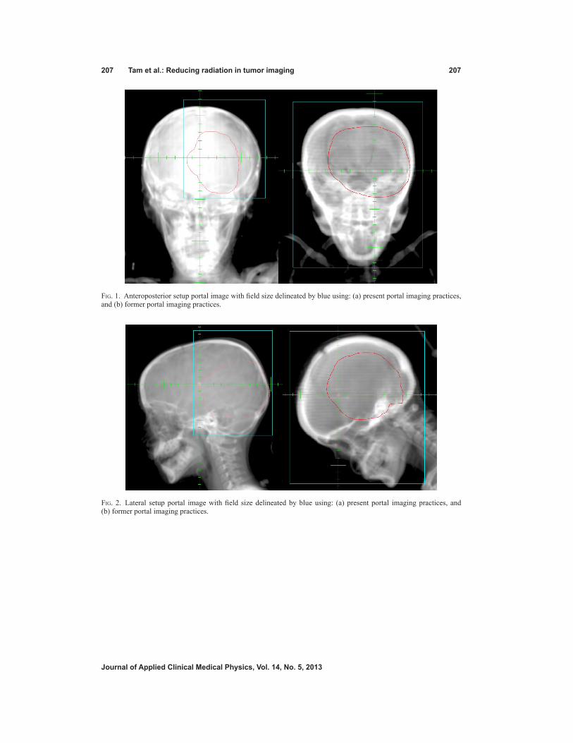
207 tam et al.: Reducing radiation in tumor imaging 207
Journal of Applied clinical Medical Physics, Vol. 14, no. 5, 2013
Fig. 1. Anteroposterior setup portal image with field size delineated by blue using: (a) present portal imaging practices, and (b) former portal imaging practices.
Fig. 2. Lateral setup portal image with field size delineated by blue using: (a) present portal imaging practices, and (b) former portal imaging practices.

208 tam et al.: Reducing radiation in tumor imaging 208
Journal of Applied clinical Medical Physics, Vol. 14, no. 5, 2013
III. RESuLtS
Table 1 lists the prescription dose (median, range, dose per fraction) and the different treatment sites (brainstem, nonbrainstem, CSI, other) for the 20 patients imaged utilizing the former portal imaging practices and the 20 patients imaged using the present imaging practices.
Table 2 shows the number of portal images and the imaging monitor units for the former cohort and the present cohort. The number of PI per patient, number of PI per fraction, number of imaging monitor units per patient, and number of imaging monitor units per fraction are listed for each cohort. Using the present portal imaging practices, patients received significantly fewer portal images per fraction (p = 0.002) compared with the patients using the former imag-ing practices. Patients imaged with the present practices also received fewer imaging monitor units (p < 0.001) and less imaging monitor units per fraction (p = 0.001).
Table 3 demonstrates the mean maximum PI dose (expressed as cGy) to OARs for patients treated using the former portal imaging practices and the present portal imaging practices. The present portal imaging practices resulted in a significant reduction in dose delivered to the optic nerves and chiasm (35%), cochlea (35%), hypothalamus (51%), temporal lobes (45%), thyroid (80%), and eyes (55%).
Table 4 reports the mean maximum PI dose expressed as a percentage of the prescribed dose to PTVs and OARs. Using the present portal imaging practices, significantly less PI dose was delivered to the PTVmean (1.0%), PTVmax (1.1%), and PTVmin (0.6%), as well as to the brainstem (0.6%), optic nerves and chiasm (0.8%), cochlea (0.9%), hypothalamus (0.8%), temporal lobes (1.0%), thyroid (1.3%), and eyes (1.4%).
Fig. 3. Example of a treatment field portal image. Using current practices, only a single exposure was taken of the treatment field through the completely irradiated aperture outline (CIAO), as represented by the blue line. Using former practices, an additional second exposure was taken of the treatment field plus 4 cm, as represented by the entire image.

209 tam et al.: Reducing radiation in tumor imaging 209
Journal of Applied clinical Medical Physics, Vol. 14, no. 5, 2013
Table 1. Treatment details.
Former PI Practice Present PI Practice
Prescription Dose Median (cGy) 5490 5580 Range (cGy) 4500–5940 3000–5940 Dose/fraction 180 180a
Treatment Sites Brainstem 7 6 Nonbrainstem 6 6 CSIb 4 6 Other 3 2
a Exception of 1 patient who received 150 cGy/fraction.b CSI used static lateral step brain fields with multileaf collimators.
Table 2. Mean number of portal images (PI) and imaging monitor units (MUs).
Former PI Practice Present PI Practice p-value
No. PI/Patient 58.8 39.7 0.001No. PI/Fraction 1.9 1.3 0.002MU/Patient 173.3 97.9 <0.001MU/Fraction 5.6 3.2 0.001
Table 3. Maximum PI dose (expressed as cGy) to OARs.
Former PI Practice Present PI Practice Change (%) p-value
OARs Brainstem 153 115 25 0.072 Optic nerves and chiasm 149 97 35 0.011 Cochlea 144 94 35 0.018 Hypothalamus 132 64 51 0.006 Temporal Lobes 124 69 45 <0.001 Thyroid 85 17 80 <0.001 Eyes 146 66 55 <0.001
Table 4. Maximum PI dose (expressed as percentage of prescribed dose) to PTV and OARs.
Former PI Practice Present PI Practice Change (%) p-value
PTV Mean 2.5 1.5 40 0.001 Min 2.2 1.6 28 0.009 Max 2.9 1.8 39 0.001OARs Brainstem 2.8 2.2 23 0.110 Optic nerves and chiasm 2.6 1.8 30 0.021 Cochlea 2.6 1.7 32 0.029 Hypothalamus 2.4 1.6 34 0.016 Temporal Lobes 2.3 1.3 43 0.001 Thyroid 1.6 0.3 80 <0.001 Eyes 2.6 1.2 56 <0.001

210 tam et al.: Reducing radiation in tumor imaging 210
Journal of Applied clinical Medical Physics, Vol. 14, no. 5, 2013
IV. dIScuSSIon
Radiation therapy is an important component of multimodality therapy for childhood CNS malignancies and has contributed to the total percentage of long-term survivors. An analysis of the Surveillance Epidemiology and End Results program showed that among survivors of childhood cancers, 24% have survived more than 30 years since their diagnosis.(6) Among this group, patients with brain cancer make up the largest number of survivors. Therefore, long-term morbidity and mortality have become increasingly important.
Our previous study revealed that radiation dose delivered from portal imaging of pediatric brain tumor patients is on average 2%–3% of the total prescribed dose for both PTV and the surrounding OARs, which is equivalent to an additional 0.5–1.0 fraction of radiation treatment. This radiation dose is typically not considered during treatment planning or documented in the dose distributions or dose-volume histograms. This additional dose delivered could easily exceed the tolerance limit of the surrounding OARs.(7,8) Of note, the eye lens has been shown to be one of the most radiosensitive tissues in the body, and some recent studies suggest that cataract development may occur at a threshold of 0.5 Gy or even a linear, no-threshold model.(9) Our study shows that the present PI practices can significantly reduce the mean PI dose to the eye from portal imaging from 146 cGy to 66 cGy. Furthermore, the thyroid experienced the most dramatic decrease of 80% in mean PI dose, from 85 cGy to 17 cGy.
Radiation exposure contributes to an increased risk of long-term morbidity and late mortality in patients with CNS malignancies. A study on survivors of medulloblastoma showed that both younger patients and higher doses are correlated with lower performance in neuropsychologic functioning.(10) A more recent study of 1887 patients with childhood CNS tumors and a median follow up of 19.6 years showed an increased risk of developing subsequent neoplasms and neurocognitive impairment.(5) The cumulative incidence of secondary neoplasm within the CNS was also associated with the maximum cranial RT dose.(5) Furthermore, cranial radia-tion therapy dose was correlated with a decreased neurocongitive functioning in survivors of astrocytoma and glial tumors. Therefore, it may be important to reduce unnecessary radiation dose from portal imaging for pediatric brain tumors.
This study shows that new practices in the use of portal imaging can be implemented to reduce the radiation exposure that is typically unaccounted. The mean additional PI dose expressed as a percentage of the prescribed dose can be reduced by 28%–80% dose for both PTVs and sur-rounding OARs. This was achieved with simple modifications to our portal imaging practices, which used smaller setup field sizes and single exposure imaging of the treatment field rather than double-exposure imaging. It must be noted that reductions in setup field size and the use of single exposure were not performed consistently for each treatment. Therefore, additional reductions in portal imaging radiation exposure may be achieved. Additionally, the present portal imaging practices did not compromise patient care. None of these 20 pediatric patients required reimaging or a second setup.
Although this study focuses on MV imaging, the use of kilovoltage (kV) imaging is another imaging technique that would reduce the dose delivered to OARs and PTVs through portal imag-ing. However, kV imaging does not completely spare normal tissue to radiation and therefore the results of this paper may also be relevant.(11-13)
V. concLuSIonS
Our changes in portal imaging practices reduced the radiation dose contribution from PI to sur-rounding OARs by up to 80%. This may have implications on both late toxicity and secondary cancer development in pediatric brain tumors.
211 tam et al.: Reducing radiation in tumor imaging 211
Journal of Applied clinical Medical Physics, Vol. 14, no. 5, 2013
AcknowLEdgMEntS
This study did not receive any direct funding or grants.
REFEREncES
1. Mueller S and Chang S. Pediatric brain tumors: current treatment strategies and future therapeutic approaches. Neurotherapeutics. 2009;6(3):570–86.
2. Hitchen CJ, Osa EO, Dewyngaert JK, Chang J, Narayana A. Dose to craniofacial region through portal imaging of pediatric brain tumors. J Appl Clin Med Phys. 2012;13(1):3385.
3. Merchant TE, Conklin HM, Wu S, Lustig RH, Xiong X. Late effects of conformal radiation therapy for pediatric patients with low-grade glioma: prospective evaluation of cognitive, endocrine, and hearing deficits. J Clin Oncol. 2009;27(22):3691–97.
4. Merchant TE, Rose SR, Bosley C, Wu S, Xiong X, Lustig RH. Growth hormone secretion after conformal radia-tion therapy in pediatric patients with localized brain tumors. J Clin Oncol. 2011;29(36):4776–80.
5. Armstrong GT, Liu Q, Yasui Y, et al. Long-term outcomes among adult survivors of childhood central nervous system malignancies in the Childhood Cancer Survivor Study. J Natl Cancer Inst. 2009;101(13):946–58.
6. Mariotto AB, Rowland JH, Yabroff KR, et al. Long-term survivors of childhood cancers in the United States. Cancer Epidemiol Biomarkers Prev. 2009;18(4):1033–40.
7. Emami B, Lyman J, Brown A, et al. Tolerance of normal tissue to therapeutic irradiation. Int J Radiat Oncol Biol Phys. 1991;21(1):109–22.
8. Stewart FA, Akleyev AV, Hauer-Jensen M, et al. ICRP PUBLICATION 118: ICRP statement on tissue reactions and early and late effects of radiation in normal tissues and organs – threshold doses for tissue reactions in a radiation protection context. Ann ICRP. 2012;41(1-2):1–322.
9. Ainsbury EA, Bouffler SD, Dörr W, et al. Radiation cataractogenesis: a review of recent studies. Radiat Res. 2009;172(1):1–9.
10. Mulhern RK, Kepner JL, Thomas PR, Armstrong FD, Friedman HS, Kun LE. Neuropsychologic functioning of survivors of childhood medulloblastoma randomized to receive conventional or reduced-dose craniospinal irradiation: a Pediatric Oncology Group study. J Clin Oncol. 1998;16(5):1723–28.
11. Ding GX and Coffey CW. Radiation dose from kilovoltage cone beam computed tomography in an image-guided radiotherapy procedure. Int J Radiat Oncol Biol Phys. 2009;73(2):610–17.
12. Waddington SP and McKenzie AL. Assessment of effective dose from concomitant exposures required in veri-fication of the target volume in radiotherapy. Br J Radiol. 2004;77(919):557–61.
13. Gu J, Bednarz B, Xu XG, Jiang SB. Assessment of patient organ doses and effective doses using the VIP-Man adult male phantom for selected cone-beam CT imaging procedures during image guided radiation therapy. Radiat Prot Dosimetry. 2008;131(4):431–43.

a Corresponding author: Sherry C. Ng, G30 Professorial Block, Queen Mary Hospital 102 Pokfulam Road, Hong Kong; phone: +852 2255 4507; fax: +852 2255 4916; email: [email protected]
Patient dosimetry for 90Y selective internal radiation treatment based on 90Y PET imaging
Sherry C. Ng,1a Victor H. Lee,2 Martin W. Law,3 Rico K. Liu,1 Vivian W. Ma,3 Wai Kuen Tso,3 To Wai Leung1
Department of Clinical Oncology,1 Queen Mary Hospital, Hong Kong; Department of Clinical Oncology,2 University of Hong Kong, Hong Kong; Department of Diagnostic Radiology,3 Queen Mary Hospital, Hong [email protected]
Received 16 January, 2013; accepted 28 March, 2013
Until recently, the radiation dose to patients undergoing the 90Y selective internal radiation treatment (SIRT) procedure is determined by applying the partition model to 99mTc MAA pretreatment scan. There can be great uncertainty in radiation dose calculated from this approach and we presented a method to compute the 3D dose distributions resulting from 90Y SIRT based on 90Y positron emission tomography (PET) imaging. Five 90Y SIRT treatments were retrospectively analyzed. After 90Y SIRT, patients had 90Y PET/CT imaging within 6 hours of the procedure. To obtain the 3D dose distribution of the patients, their respective 90Y PET images were convolved with a Monte Carlo generated voxel dose kernel. The sensitivity of the PET/CT scanner for 90Y was determined through phantom studies. The 3D dose distributions were then presented in DICOM RT dose format. By applying the linear quadratic model to the dose data, we derived the biologically effective dose and dose equivalent to 2 Gy/fraction delivery, taking into account the spatial and temporal dose rate variations specific for SIRT. Based on this data, we intend to infer tumor control probability and risk of radiation induced liver injury from SIRT by comparison with established dose limits. For the five cases, the mean dose to target ranged from 51.7 ± 28.6 Gy to 163 ± 53.7 Gy. Due to the inhomogeneous nature of the dose distribution, the GTVs were not covered adequately, leading to very low values of tumor control probability. The mean dose to the normal liver ranged from 21.4 ± 30.7 to 36.7 ± 25.9 Gy. According to QUANTEC recommenda-tion, a patient with primary liver cancer and a patient with metastatic liver cancer has more than 5% risk of radiotherapy-induced liver disease (RILD).
PACS number: 87.53.Bn
Key words: yttrium-90 microsphere, liver cancer, PET, dosimetry, LQ model
I. InTroducTIon
Selective Internal Radiation Treatment (SIRT) is the delivery of radiation treatment via intra-hepatic arterial administration of 90Y microspheres. 90Y SIRT is an emerging modality in the management of patients with inoperable primary and metastatic liver cancer. It is based on the unique pattern of hepatic blood flow by which the majority of the tumor blood supply is derived from the hepatic artery, whereas hepatic parenchymal blood flow largely comes from the portal vein. When 90Y microspheres are introduced through the hepatic artery, 90Y microspheres will preferentially localize in the peritumoral and intratumoral arterial vasculature, delivering high dose of radiation to the tumors. The use of 90Y microspheres for treatment of liver neoplasms has been around for some time; prospective clinical trials have shown encouraging response and survival data.(1)
JournAL oF APPLIEd cLInIcAL MEdIcAL PHYSIcS, VoLuME 14, nuMBEr 5, 2013
212 212

213 ng et al.: SIrT dosimetry from 90Y PET imaging 213
Journal of Applied clinical Medical Physics, Vol. 14, no. 5, 2013
Until now, the radiation dose for the SIRT procedure was estimated by the partition method based on pretreatment 99mTc MAA diagnostic angiogram.(2,3) However, there are great uncertain-ties associated with this approach. The reproducibility of catheter positioning during therapy is questionable and the particle size of 90Y microsphere is different from that of 99mTc MAA, so the distribution of 99mTc MAA may not truly correspond to that of 90Y microsphere.
In radionuclide therapy, the absorbed dose is usually estimated, because in vivo dose mea-surement is not feasible in clinical settings. However, without accurate patient dosimetry, it is impossible to establish fundamental dose-response relationship for treatment efficacy and toxicity. Also, it is difficult for different institutes to compare treatment results. For SIRT treat-ments, there is great inhomogeneity of 90Y concentration within the patient’s body and, because of the short range of the 90Y beta particles, the total dose and dose rate vary spatially over the irradiated volume. The dose rate also changes temporally as the 90Y decays. The spatial and temporal variations of dose rate will have different radiobiological effect on the tumor and normal tissues. The partition method assumes a uniform distribution of 90Y microsphere, disregarding the spatial and temporal variation of the dose and dose rate. Consequently, the radiobiological effects specific to SIRT are ignored, and the partition method is at best a simplified picture for the patient dosimetry.
90Y has an internal pair production component with a branching ratio of 31.87 ± 0.47 × 10⁻⁶.(4) Recently, this pair production component of 90Y decay for PET imaging has been employed to evaluate the distribution of 90Y for patients treated with SIR-Spheres.(5) The image quality of 90Y PET is superior to the traditional Bremsstrahlung SPECT and correlates well to the diag-nostic 18FDG PET and CT scan. In this paper, we computed patient dose from 90Y SIR-Spheres based on high-quality 90Y PET images. This makes possible the calculation of accurate 3D physical dose distributions.
Considering the radiobiological effect of varying dose rates, tumor control probability and normal liver dose constraints should not be directly applied to the physical dose data. We used the linear quadratic (LQ) model to convert the physical dose to the biologically effective dose (BED). The BED was then converted to dose equivalent to delivery at 2 Gy/fraction (EQ2), which is the typical dose per fraction used in conventional external beam radiation therapy and upon which published limits for tumor control and normal tissue complication are usually based. With EQ2, the application of dose limits to tumor control and normal tissue are meaningful.
II. MATErIALS And METHodS
A. Absorbed dose from 99mTc MAA scintigraphyFrom January 2011 to March 2012, five patients (all male, aged 45–78 years) who received SIRT had subsequent 90Y PET scan in our institute. Three patients had inoperable hepatocellular carcinoma, the other two (patients 1 and 3) had inoperable metastatic liver cancer from primary colorectal cancer. All patients met the manufacturer’s assessment criteria for SIRT. Diagnostic whole body 18FDG PET/CT was done to assess the tumor extent and target localization. Prior to SIRT, arteriography, followed by 99mTc-labeled MAA scintigraphy, was performed on all patients to assess the hepatic arterial vasculature and also for hepatopulmonary shunt fraction calculation. It also detected any gastrointestinal reflux, if present. Whole body anterior and posterior planar images of the chest and abdomen were taken after infusion of 4 mCi of 99mTc MAA. Based on the 99mTc MAA distribution, absorbed dose was calculated with the partition method. The tumor absorbed dose, Dt, and normal liver absorbed dose, Dl, can be calculated from Eq. (1) and (2):(2)
(1)
Dt 49.8
A (GBq)M (kg)
r1 (Mt/M)(r 1)

214 ng et al.: SIrT dosimetry from 90Y PET imaging 214
Journal of Applied clinical Medical Physics, Vol. 14, no. 5, 2013
(2)
D1 49.8
A (GBq)M (kg)
11 (Mt/M)(r 1)
Here, A is the administered activity, M is the mass of the liver, Mt is the mass of tumor, and r is the tumor/liver activity uptake ratio determined from the scintigraphy. The tumor/liver activity uptake ratio, r, was calculated as (counts from tumor ROI)/(counts from normal liver ROI).
B. calibration of PET/cT scanner for 90YTo obtain the activity concentration of 90Y within the patients’ bodies, sensitivity of the PET scanner for 90Y was determined. Calibration of the PET/CT scanner for the 90Y isotope was performed with a rectangular phantom containing four spherical inserts containing 90Y solu-tion in a cold background. 90Y solution was used instead of 90Y SIR-Spheres because the SIRT spheres tend to settle over time during imaging, resulting in an uneven distribution of 90Y within the spherical inserts. This could affect calibration accuracy. The inserts were filled with a nominal activity concentration of 2.996 MBq/ml of 90Y. The volume of the spheres ranged from 0.22 cm3 to 65.45 cm3, whereas the background volume was 8.26 liters. (See Fig. 1 for the PET/CT image of the calibration phantom.)
c. dosimetry from 90Y PET/cT imaging90Y PET/CT imaging was performed with GE Discovery STE PET/CT scanner (GE Healthcare, Waukesha, WI) within 6 hours of the SIRT procedure. Attenuation corrected 90Y PET images were collected at two bed positions 30 minutes each, covering the whole liver and lung base. For a known activity distribution in a homogeneous tissue of infinite extend, the spatial dose distribution can be determined by convolving the nuclide concentration (from the PET images in our case) with the dose point kernel, described in the following:(6)
D• (r) A(r) k(r) (3)
Here D• (r) is the absorbed dose rate at point r, A(r) is the cumulative activity at point r, and k(r) is the dose point kernel. The Medical Internal Radiation Dose (MIRD) Committee calcu-lated S values at the voxel level for several relevant radionuclides using EGS4.(7) In this study,
Fig. 1. PET/CT image (a) of the calibration phantom. Variation (b) of the observed mean activity concentration for each spherical insert with the volume of the inserts.

215 ng et al.: SIrT dosimetry from 90Y PET imaging 215
Journal of Applied clinical Medical Physics, Vol. 14, no. 5, 2013
we used the published S values presented in MIRD Pamphlet 17(7) of 6 mm voxels for 90Y in a homogeneous medium.
Based on the calibration, the observed count rate for each voxel on the PET images was converted to the activity concentration for the 90Y distribution. The voxel size of the PET images was 5.47 × 5.47 × 3.27 mm3, therefore the 6 mm voxel point dose kernel from Bolch et al.(7) was first resampled to voxel size equivalent to the PET image voxel size for convolution. Figure 2 shows the two-dimensional representation of the resampled voxel point dose kernel which was subsequently convolved with the PET images to compute the instantaneous dose rate. The three-dimensional convolution was done in MATLAB (The MathWorks, Natick, MA; www.MathWorks.com). The resultant values were again resampled to voxel size of 2.5 × 2.5 × 2.5 mm3 to match the voxel size of the CT images. Then by integrating the decaying dose rate to infinity, we obtained the total dose delivered to each voxel. DICOM-RT dose files were generated corresponding to the dose values. (See Fig. 3 for the dose distribution (Fig. 3(a)) and 90Y PET/CT image (Fig. 3(b)) of patient 1).
For DVH computation, the target and organ at risk need to be localized. For each patient, the liver was localized on the 90Y PET/CT images. The target was localized on the diagnos-tic 18FDG PET/CT images by radiation oncologists. The diagnostic 18FDG PET/CT images were registered to the 90Y PET/CT images and target copied to the 90Y PET/CT images for DVH computation.
Fig. 2. Resampled voxel dose kernel to match the voxel size of the PET images.
Fig. 3. 90Y PET image (a) 5 hours after treatment. Red contours indicate position of the target as localized by radiation oncologist based on diagnostic 18FDG PET/CT. 90Y is localized in the left lobe of the liver; very little activity is seen in the lung base. 90Y PET-based isodose map (b) from PET image of (a).

216 ng et al.: SIrT dosimetry from 90Y PET imaging 216
Journal of Applied clinical Medical Physics, Vol. 14, no. 5, 2013
d. computation of biologically effective dose and dose equivalent to 2 Gy per fraction delivery
Once injected into the hepatic artery, the microspheres are distributed preferentially in the tumor areas, being trapped within the tumor microvasculature. There is very little biological clearance and 90Y decays with its physical half-life of 2.67 days. The 90Y microspheres become permanent implants. There are two considerations in applying the physical dose calculated from above to assess tumor control and the risk of radiotherapy-induced liver disease (RILD). Firstly, the delivery dose rate is changing, starting at maximum at the embolization procedure (can reach 4 Gy per hour for our group of patients), exponentially dropping to almost zero in ten half-lives. Secondly, the total dose and the dose rate are inhomogeneous throughout the target volume and organ-at-risk (OAR) volume. Thus the biological effect of the dose is also varying throughout the target volume and the OAR. It will be incorrect to compare the physical dose computed from the 90Y PET images directly with published data for tumor control and risk of RILD, when published data for radiation dose of tumor control and radiation-associated injury is often derived from external beam therapy data, most likely in fractionation of 2Gy/fraction.
The biologically effective dose (BED) is defined in terms of both physical and radiobiologi-cal parameters, and is a measure of the total amount of lethal damage sustained by a specific tissue. The BED is obtained by multiplying the total physical dose with a modifying factor which takes into account the physical aspects of dose delivery (dose rate, dose per fraction). For a permanent implant delivering an initial dose rate of Ro, and involving a nuclide with decay constant λ, Eq. (4) gives the BED.(8) Here μ is the time constant for sublethal damage repair.(9) Since the 90Y microspheres are trapped in the capillary bed, there is virtually no biological clearance and 90Y decays with its physical half-life of 2.67 days, λ = 0.2596 d-1. μ = log2/T1/2 is the repair constant for the repair of sublethal damage. Repair T1/2 for tumors and normal tissues are less well established than α/β, and from Gerbaulet et al.,(10) T1/2 = 30 min to 1 h for early-reacting normal tissues and tumors, and T1/2 = 1.5 h for late-reacting normal tissues. We used T1/2 = 1 h for tumor and T1/2 = 1.5 h for healthy liver in our study.
(4)
BEDRO 1
RO
The initial dose rate Ro is given by total dose divided by the decay constant λ. Making use of this equation and the differential dose-volume histogram (dDVH), we con-
verted the physical dose dDVH to the BED dDVH. Then the BED dDVH was converted to equivalent doses as if given as fractionated irradiation at 2Gy/fraction by Eq. (5). Here we were using α/β = 2.5 Gy for normal liver and α/β = 10 Gy for tumor, values taken from Gerbaulet et al.:(10)
(5)
ndBED
1 d
where nd is the total dose corresponding to dose delivered at d = 2 Gy fractions. We denoted this dose as EQ2.

217 ng et al.: SIrT dosimetry from 90Y PET imaging 217
Journal of Applied clinical Medical Physics, Vol. 14, no. 5, 2013
E. computation of tumor control probabilityTo calculate the overall tumor control probability based on the differential volume histogram, for each dose bin of the dDVH, of volume Vi receiving a dose Di, with clonogenic density ρi, the tumor control probability can be written as:(11)
TCPi exp[ iViexp( Di)] (6)
Here, α is the sensitivity of the tumor cells to radiation.Then the total tumor control probability can be found by multiplying the individual TCPs
together, and so:
TCP ∏i[exp iViexp( Di)]
(7)
In Eq. (7), α equals to 0.33 Gy-1,(12) and we assumed α value is constant (all the tumor cells have the same sensitivity). The clonogenic density ρi is equal to 107.(13)
III. rESuLTS
Sensitivity of our PET scanner for the 90Y isotope was determined by phantom study. Figure 1(a) shows the calibration phantom and Fig. 1(b) is the variation of the observed mean activity concentration for each spherical insert with the volume of the inserts. The quality of the PET/CT image of the phantom was excellent, even the 0.22 cm3 sphere was visible. Each sphere was contoured and average activity concentration determined. The average activity concentra-tions were plotted against the volume of spheres and result showed in Fig. 1(b). The dotted line showed the fitted data. Sensitivity of our PET scanner was found to be 0.32 cps/MBq.
From December 2010 to March 2012, five patients had SIRT treatment in our institution with 90Y PET imaging done within 6 hours after SIRT. Patients 2 and 3 suffered from meta-static liver cancer, patients 1, 4, and 5 had hepatocellular carcinoma. Figure 3(a) shows the 90Y PET image of patient 1 who suffered from inoperable multifocal hepatocarcinoma. 1.3 GBq of 90Y SIR-Spheres (SIRTeX Medical Limited, Sydney, Australia) was administered via a Fr3 Progreat microcatheter (Terumo Medical Corp., Somerset, NJ) inserted into Fr5 Yashiro catheter (Terumo Medical Corp.) at the hepatic proper artery. Then 90Y PET imaging was performed 5 hours afterwards. PET images showed the presence of hot spots in areas close to or within the target delineated by the radiation oncologist on the diagnostic 18FDG PET/CT images. Based on the 90Y PET images, the dose to the patients was computed. Figure 3(b) shows the resultant isodose distribution. For this patient, the mean dose to the target and normal liver was 112.5 ± 47.6 Gy and 25.8 ± 28.1 Gy, respectively.
For the five patients, we also computed the dose to target and dose to normal liver based on the partition method using Eqs. (1) and (2). Figure 4 shows a comparison of the dose cal-culated from the partition method and 90Y PET-based patient dosimetry for these five patients. Based on the differential dose-volume histograms for target and normal liver and using Eqs. (4) and (5), the BED DVH and the EQ2 DVH were computed. Figure 5 shows the DVHs of target and normal liver for patient 1. Table 1 shows the dose to target and normal liver for all the patients.
Using Eq. (7), we tried to compute the TCP for the five patients. A MATLAB program was written to do the computation based on the dDVHs. However, due to the inhomogeneous nature of SIRT, substantial cold spots were found in the target of all the patients and the calculated TCP were effectively zero for all the patients.
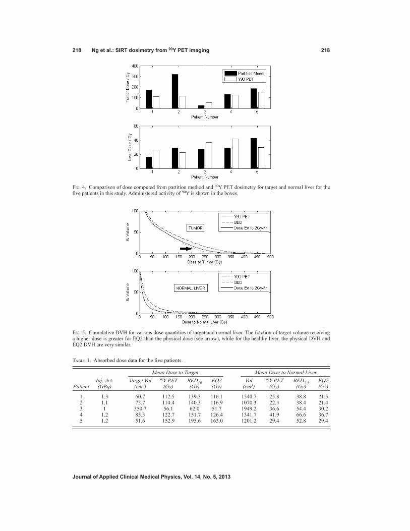
218 ng et al.: SIrT dosimetry from 90Y PET imaging 218
Journal of Applied clinical Medical Physics, Vol. 14, no. 5, 2013
Fig. 4. Comparison of dose computed from partition method and 90Y PET dosimetry for target and normal liver for the five patients in this study. Administered activity of 90Y is shown in the boxes.
Fig. 5. Cumulative DVH for various dose quantities of target and normal liver. The fraction of target volume receiving a higher dose is greater for EQ2 than the physical dose (see arrow), while for the healthy liver, the physical DVH and EQ2 DVH are very similar.
Table 1. Absorbed dose data for the five patients.
Mean Dose to Target Mean Dose to Normal Liver Inj. Act. Target Vol 90Y PET BED10 EQ2 Vol 90Y PET BED2.5 EQ2 Patient (GBq) (cm3) (Gy) (Gy) (Gy) (cm3) (Gy) (Gy) (Gy)
1 1.3 60.7 112.5 139.3 116.1 1540.7 25.8 38.8 21.5 2 1.1 75.7 114.4 140.3 116.9 1070.3 22.3 38.4 21.4 3 1 350.7 56.1 62.0 51.7 1949.2 36.6 54.4 30.2 4 1.2 85.3 122.7 151.7 126.4 1341.7 41.9 66.6 36.7 5 1.2 51.6 152.9 195.6 163.0 1201.2 29.4 52.8 29.4

219 ng et al.: SIrT dosimetry from 90Y PET imaging 219
Journal of Applied clinical Medical Physics, Vol. 14, no. 5, 2013
IV. dIScuSSIon
In this work, we presented a method of patient dosimetry for the SIRT procedure based on 90Y PET/CT imaging which is practicable in a clinical setting. 90Y PET is a reliable method for the assessment of SIR-Sphere distribution with superior image quality compared to 90Y Bremstrahlung scan. We computed the patients’ three-dimensional dose distributions based on these high-resolution PET images and represented in DICOM-RT dose file format. In addition, the CT images provide additional anatomical information so that dose to other structures can be computed as required.
Sensitivity of the PET scanner was determined through phantom study. Sensitivity of our PET scanner for 90Y was found to be 0.32 cps/MBq. Werner et al.(14) determined the sensitivity of 90Y for their Siemens Biograph 16 HiRez PET scanner at 40 min/bed to be 0.72 cps/MBq, which is comparable to our results. Several studies have used partition model based on 99mTc MAA scans to compute the dose to tumor and normal liver for the 90Y SIRT procedure.(2,13) These approaches assumed uniform distribution of activity within each partition and only give an estimate of the dose received in each compartment. One other study has used an approach similar to ours to calculate the radiation absorbed dose for 90Y SIRT of an HCC patient. Sarfaraz et al.(15) convolved the 99mTc MAA SPECT image with a Monte Carlo generated voxel dose kernel to compute the dose distribution from the 90Y spheres. However, dosimetry based on 99mTc MAA SPECT imaging has two major drawbacks. First, the difference in particle size of 99mTc MAA from the 90Y microspheres (MAA particles have diameters in the range 15 to 30 microns and a density of 1.3 g/cc, and SIR-Sphere microspheres have diameters of 35 ± 5 microns and a density of 1.6 g/cc(16)), and thus the distributions of the two types of particles are not identical. Secondly, there is uncertainty arising from catheter placement for 99mTc MAA and 90Y SIRT which are, in fact, two separate procedures. Our results showed large discrepancies between the doses calculated based on partition method and 90Y PET dosimetry, especially the dose to the target (difference ranged from -53.8% to +178.4%). For the tumor, partition method generally overestimated the dose. Other than the fundamental differences between these two dose calculation methods, the large discrepancy for target dose arises from inconsistency of target localization. The partition method relies on the accuracy of the tumor to liver uptake ratio, r. For our study, this ratio is determined from planar 99mTc MAA scintigraphy for which the tumor and liver were localized on the 2D images. On the other hand, the target volume for the 90Y PET dosimetry is based on diagnostic 18FDG PET/CT. Disagreement of target localization between the two approaches is to be expected, resulting in considerable difference in dose to target for the two methods.
The SIR-Spheres are classified by regulators as a brachytherapy medical device, and radi-oembolization with SIR-Spheres is effectively permanent implant brachytherapy. As discussed above, there is great dose inhomogeneity due to the way the 90Y microspheres are introduced into the patient’s body, and also due to rapid dose falloff with distance from the sources. As 90Y decays, the dose rate will also change with time. The spatial and temporal variation of dose rate will have varying radiobiological effects on tumor control and normal liver sparing. The effect of these variations cannot be reflected if only the physical dose is reported. Also, because of the dose gradient, each voxel of the target and healthy liver will be receiving a different total dose at a different time, varying dose rate. Applying the LQ model to the mean dose of the target or healthy liver to get the mean BED is oversimplification. Thus, we applied the LQ model to the differential dose-volume histogram, calculating the BED and EQ2 dose for each dose bin within which the dose and dose rate is relatively constant. This will give us the BED dDVH and EQ2 dDVH. It was based upon these results that we computed the mean BED and mean EQ2 dose to the target and normal liver for each patient. Table 1 shows the mean physical dose, BED, and EQ2 for the target and normal liver. For the five patients, the mean dose to the target ranged from 51.7 ± 28.6 to 163 ± 53.7 Gy. Due to the inhomogeneous nature of the dose distribution, there were significant geographic misses of the target, leading
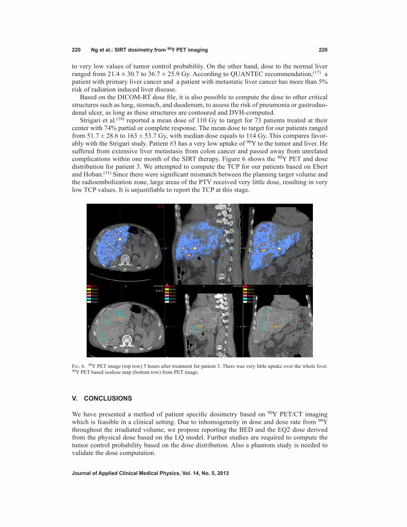
220 ng et al.: SIrT dosimetry from 90Y PET imaging 220
Journal of Applied clinical Medical Physics, Vol. 14, no. 5, 2013
to very low values of tumor control probability. On the other hand, dose to the normal liver ranged from 21.4 ± 30.7 to 36.7 ± 25.9 Gy. According to QUANTEC recommendation,(17) a patient with primary liver cancer and a patient with metastatic liver cancer has more than 5% risk of radiation induced liver disease.
Based on the DICOM-RT dose file, it is also possible to compute the dose to other critical structures such as lung, stomach, and duodenum, to assess the risk of pneumonia or gastroduo-denal ulcer, as long as these structures are contoured and DVH-computed.
Strigari et al.(18) reported a mean dose of 110 Gy to target for 73 patients treated at their center with 74% partial or complete response. The mean dose to target for our patients ranged from 51.7 ± 28.6 to 163 ± 53.7 Gy, with median dose equals to 114 Gy. This compares favor-ably with the Strigari study. Patient #3 has a very low uptake of 90Y to the tumor and liver. He suffered from extensive liver metastasis from colon cancer and passed away from unrelated complications within one month of the SIRT therapy. Figure 6 shows the 90Y PET and dose distribution for patient 3. We attempted to compute the TCP for our patients based on Ebert and Hoban.(11) Since there were significant mismatch between the planning target volume and the radioembolization zone, large areas of the PTV received very little dose, resulting in very low TCP values. It is unjustifiable to report the TCP at this stage.
V. concLuSIonS
We have presented a method of patient specific dosimetry based on 90Y PET/CT imaging which is feasible in a clinical setting. Due to inhomogeneity in dose and dose rate from 90Y throughout the irradiated volume, we propose reporting the BED and the EQ2 dose derived from the physical dose based on the LQ model. Further studies are required to compute the tumor control probability based on the dose distribution. Also a phantom study is needed to validate the dose computation.
Fig. 6. 90Y PET image (top row) 5 hours after treatment for patient 3. There was very little uptake over the whole liver. 90Y PET based isodose map (bottom row) from PET image.
221 ng et al.: SIrT dosimetry from 90Y PET imaging 221
Journal of Applied clinical Medical Physics, Vol. 14, no. 5, 2013
rEFErEncES
1. Gary BN, Anderson JE, Burton MA, et al. Regression of liver metastases following treatment with yttrium-90 microspheres. Aust N Z J Surg. 1992;62(2):105–10.
2. Lau WY, Ho S, Leung WT, et.al. Selective internal radiation therapy for nonresectable hepatocellular carcinoma with intraarterial infusion of 90yttrium microspheres. Int J Radiat Oncol Biol Phys. 1998;40(3):583–92.
3. Miller WT. Application of the linear-quadratic model with incomplete repair to radionuclide directed therapy. Brit J Radiol. 1991;64(759):242–51.
4. Gates V, Eesmail A, Marshall K, Spies S, Salem R. Internal pair production of 90Y permits hepatic localization of microspheres using routine PET: proof of concept. J Nucl Med. 2011;52(1):72–76.
5. Lhommel R, Goffette P, Van den Eynde M, et al. Yttrium-90 TOF PET scan demonstrates high-resolution biodis-ribution after liver SIRT. Eur J Nucl Med Mol Imaging. 2009;36(10):1696.
6. Kolbert K, Sgouros G, Scott AM, et al. Implementation and evaluation of patient-specific three-dimensional internal dosimetry. J Nucl Med. 1997;38(2):301–08.
7. Bolch WH, Boucher LG, Robertson JS, et al. MIRD Pamphlet No.17: The dosimetry of nonuniform activity distributions – radionclide S values at the voxel level. Medical Internal Radiation Dose Committee. J Nucl Med. 1999;40(1):11S–136S.
8. Dale RG and Jones B. The clinical radiobiology of brachytherapy. Brit J Radiol. 1998;71(845):465–83. 9. Dale RG. The application of the linear-quadratic dose-effect equation to fractionated and protracted radiotherapy.
Brit J Radiol. 1985;58(690):515–28. 10. Gerbaulet A, Potter R, Mazeron J, Meertens H, Limbergen EV. The GEC ESTRO Handbook of Brachytherapy.
Brussels: ESTRO; 2002. 11. Ebert MA and Hoban PW. Some characteristics of tumour control probability for heterogeneous tumours. Phys
Med Biol. 1996;41(10):2125–33. 12. Jones B and Dale RG. Radiobiological modeling and clinical trials. Int J Radiat Oncol Biol Phys.
2000;48(1):259–65. 13. Campbell J, Wong O, Muzik O, Marples B, Joiner M, Burmeister J. Early dose response to yttrium-90 micro-
sphere treatment of metastatic liver cancer by patient-specific method using single photon emission computed tomography and positron emission tomography. Int J Radiat Oncol Biol Phys. 2009;74(1):313–20.
14. Werner M, Kupferschläger J, Bever T, et al. PET/CT for the detection and quantification of the β-emitting thera-peutic radionuclide Yttrium-90 after liver SIRT [abstract]. J Nucl Med. 2010;51(Suppl 2):341.
15. Sarfaraz M, Kennedy AS, Lodge MA, Li XA, Wu X, Yu CX. Radiation absorbed dose distribution in a patient treated with yttrium-90 microspheres for hepatocellular carcinoma. Med Phys. 2004;31(9):2449–52.
16. Gulec SA, Mesoloras G, Dezarn WA, McNeillie P, Kennedy AS. Safety and efficacy of Y-90 microsphere treat-ment in patients with primary and metastatic liver cancer: the tumor selectivity of the treatment as a function of tumor to liver flow ratio. J Transl Med. 2007;5:15–24.
17. Pan C, Kavanagh B, Dawson L, et al. Radiation-associated liver injury. Int J Radiat Oncol Biol Phys. 2010;76(3 Suppl):S94–S100.
18. Strigari L, Sciuto R, Rea S, et al. Efficacy and toxicity related to treatment of hepatocellular carcinoma with 90Y-SIR spheres: radiobiologic considerations. J Nucl Med. 2010;51(9):1377–85.

a Corresponding author: Jerome Krayenbuehl, Radio-Onkologie, Rämistrasse 100 8091 Zurich, Switzerland; phone: (+41) 44 255 32 49; fax: (+41) 44 255 45 47; email: [email protected]
Hierarchical enhanced non-rigid registration for target volume correction and propagation for adaptive external beam radiotherapy of carcinoma of the prostate
Adrian Andronache,1 Jerome Krayenbuehl,2a Gabor Szekely,1 Ilja F. Ciernik3,4 Computer Vision Laboratory,1 Federal Institute of Technology, Zurich, Switzerland; Department of Radiation Oncology,2 Zurich University Hospital, Zurich, Switzerland; Department of Radiation Oncology,3 City Hospital, Dessau, Germany; Center for Clinical Research,4 Zurich University Hospital, [email protected]
Received 17 January, 2013; accepted 28 April, 2013
Volumes change during fractionated radiotherapy (RT). We investigate a tool based on the Hierarchical Enhanced Registration Algorithm (HERA) to project a 3D segmentation set of the prostate into the subsequent imaging sets at any time point during RT by using intensity-based image registration techniques. Sequential CT sets during RT at 15, 30, 45, and 60 Gy of two patients were used. Five expert clinicians outlined the prostate in a blinded fashion, defining intraobserver and interobserver variability on a set of 35 and 25 scans, respectively. The observer variability and positioning for manual correction was compared to both affine and elastic image registration-based contour propagation. The overall mean error of the registration-based correction of the planning target volume was comparable to the interobserver variability of manual target volume definition. The correction by affine image fusion was inferior to the results of elastic registration. The maximal deviation for the interobserver segmentation was 15.4 mm, 10.5 mm for the affine and 8.0 mm for the elastic registration. The mean interobserver variability was 1.5 (± 1.4) mm, 2.8 (± 2.3) mm for the affine, and 2.2 (± 1.9) mm for the elastic registration. Intensity-based elastic registration of deformable anatomical structures with HERA is suitable for the assessment of changes of prostate volumes for the purpose of target propagation and adaptive radiotherapy.
PACS number: 87.57.nj
Key words: adaptive radiotherapy, external radiotherapy, prostate cancer, non-rigid registration
I. IntroductIon
External beam radiotherapy of the prostate is generally performed over a larger number of frac-tions. Over this period, the volumes of the rectum and bladder can fluctuate causing displacement and may contribute to the deformation of the target volumes, as well. Therefore, anatomical and geometrical uncertainties must be taken into account by the planning target volume (PTV). The spatial plasticity of the prostate during the course of RT has been well documented, and the volume of the prostate may slightly increase during the first days of RT and shrink dur-ing the following weeks.(1,2) In order to keep PTV margins minimal, daily target positioning verification before treatment can be beneficial.(3) Several techniques have been investigated to account for the intertreatment positioning variability of the prostate. Before high-resolution in-room fluoroscopy or 3D on-board imaging systems became available, the localization of the
JournAL oF APPLIEd cLInIcAL MEdIcAL PHYSIcS, VoLuME 14, nuMBEr 5, 2013
222 222

223 Andronache et al.: non-rigid registration for adaptive radiotherapy 223
Journal of Applied clinical Medical Physics, Vol. 14, no. 5, 2013
prostate mostly relied on remote anatomical bony markers. Endorectal spacers help to predict the position of the prostate and could reduce internal target volume (ITV) margins.(4) Direct prostate localization is achieved with fiducial markers in the prostate.(5) Other positioning sys-tems rely on ultrasound technology or transponders.(6,7) All these approaches, however, neglect the plasticity of the target structures and volumes over the treatment time.
On-board CTs during RT provide a novel opportunity to redefine the volume of the prostate on a daily basis and, if necessary, adapt the CTV. However, the reliability of CT-based prostate localization and volume assessment may be reduced by technical limitations, such as the typical low contrast soft tissue differentiation of the common on-board CT imaging systems, interfering with resegmentation and automated target volume reconstruction.
In the present work, we investigate the possibility of using image registration techniques as a tool for target volume propagation. Image registration is the process of transforming the different sets of data onto one coordinate system, such that the scene or the objects pictured from different views and/or at different time points are brought into alignment. Considering that the physician can make a detailed planning and contouring of the prostate onto an initial CT scan of a patient, we registered it to all the subsequent CTs acquired during the RT. By using nonrigid image registration techniques such as the Hierarchical Enhanced Registration Algorithm (HERA),(8) we studied the performance of both affine and nonrigid transformations to estimate the spatial changes and to compensate for the plasticity of the pelvic structures. The information from the positioning changes of the pelvis is applied to the prostate clinical target volume (CTV), allowing precise prostate localization during potentially each single treatment sessions. The ability of the physicians to manually define the prostate volume for the purpose of adaptive radiotherapy is compared to the performance of the proposed automated computer-based CTV registration. Routine adaptation of the prostate volume and online replanning to account for volume changes during radiotherapy has not been introduced in routine treatment yet. One major requirement in implementation of adaptive image-guided radiotherapy will rely on optimal iterative target volume assessment procedure. Using a method based on ray casting, hierarchical image registration and manual segmentation is a novel approach in the context of adaptive radiotherapy. We hypothesize that the automated registration with HERA will improve the contouring of the prostate and eventually allow minimizing PTV margins for the purpose of adaptive radiotherapy, especially posteriorly, avoiding underdosing the posterior lobes of the prostate.
II. MAtErIALS And MEtHodS
A. Patient characteristics and ct acquisitionSequential CTs were obtained from two prostate cancer patients undergoing external beam radiotherapy. Patients were scanned and treated in a supine position with a rectal balloon with 40 cm3 of air.(4) CTs were obtained before starting treatment and at 15 Gy, 30 Gy, and 45 Gy for two patients and, additionally, 60 Gy for one patient. All CTs have been performed on a helical single-slice CT scanner. The slice thickness of the CT images was 5 mm for both patients. The in-plane resolution was 512 × 512 pixels of 0.9766 × 0.9766 mm2 for the first patients, and 512 × 512 pixels of 0.8301 × 0.8301 mm2 for the second patient.
B. Prostate contouring — interobserver and intraobserver segmentation variabilityThe interobserver variability of the manual prostate segmentation was defined by a group of five expert clinicians that, in a blinded fashion, manually contoured repeatedly the prostate in all seven available CTs (0 Gy, 15 Gy, 30 Gy for two patients, and 60 Gy for one patient). The manual segmentation was performed using Eclipse treatment planning system (Varian Medical Systems, Palo Alto, CA), and saved as DICOM-RT to be used in subsequent analysis. The long-term intraobserver variability was investigated by asking the same doctors to repeat the

224 Andronache et al.: non-rigid registration for adaptive radiotherapy 224
Journal of Applied clinical Medical Physics, Vol. 14, no. 5, 2013
prostate segmentation in the available CT data. The average time interval between the delinea-tion of the first and the second set of contours was about six months, in a blinded fashion. For both patients, the segmentation was done for the entire time-series of CT acquisitions (seven images) resulting in 35 CT sets for the interobserver analysis. For the intraobserver analysis, the segmentation was repeated for the acquisition prior to the RT resulting in a set of 20 CTs.
c. distance-based metricsEach CT image had a series of five manual segmentations of the prostate, each of them fur-nished a set of 2D axial contour points defined on subsequent slices of the acquisition. The average center of mass of the prostate (CMP) was estimated from all the contour points of the five segmentations, and each segmentation was reconstructed by using a simple tessella-tion procedure of the originally defined points. Then, the CMP was used as source point to radially cast 2048 rays, uniformly distributed using a constant angular step in both elevation 0° < θ ≤ 180° and azimuth 0° ≤ θ ≤ 360° directions. The average spatial location of the five intersection points between the segmented surfaces and each ray casted from the CMP was then used to estimate an average segmentation surface. At the same time, these intersection points, along each casted ray, define an estimate of the local interobserver variability (within the analyzed CT image). By putting together all these local estimates, we expressed globally the interobserver segmentation variability in terms of standard deviations of contour displace-ments within the same CT image, as delineated by the group of five clinicians.
In a similar local manner, the long-term intraobserver variability was expressed in terms of standard deviation of the contour displacements distribution estimated from the long-term repeated manual segmentations of the five clinicians on the two available CTs prior RT.
d. Image registration and contour propagationHERA was used to estimate and to correct for the plasticity of the pelvic structures between subsequent CT scans.(8) HERA optimized an affine transformation (displacement, rotation, skew, and scaling) and an elastic deformation field between the initial CT scan (prior to RT) and each subsequent CT scan (during RT) of each patient. These transformations (affine and elastic) were used eventually to propagate the prostate contour, as defined on the initial CT scan of each patient, prior to RT. The registration procedure used image intensity cross-correlation as similarity measure, as all images were acquired in the same modality (i.e., CT). In addition, to limit the influence of out of interest pelvic tissues and structures, we restricted the registration process to the prostate surrounding region.
The propagated contours were characterized by using the same ray-casting strategy as for the evaluation of the intra- and interobserver manual segmentation variability.
E. Evaluation of the contour propagation effectiveness To evaluate the precision of image registration as a propagation tool, we compared the propa-gated contours of the prostate with the segmentations obtained manually. We used different measures to locally describe and quantify the precision of the registration for each of the five CT data acquired during the RT.
In a first step, the registration-based contour propagation was compared to the interobserver variability of the prostate segmentation. Therefore, a two-tailed Student’s t-test was used on the null hypothesis that the mean (average) of the propagated contours is inside the confidence interval of the mean of the manually segmented contours, against the alternative hypothesis that the mean of the propagated contours is outside this confidence interval.
In a second step, the registration-based contour propagation was compared to the intraob-server variability. Having the CT data segmented twice by each doctor, one can compare the two populations of contour deviations originating from the same person — in one case, the contours have been generated by the same person on the same image, and in the other case, the contours have been generated by the same person on two different images and propagated

225 Andronache et al.: non-rigid registration for adaptive radiotherapy 225
Journal of Applied clinical Medical Physics, Vol. 14, no. 5, 2013
over. Therefore, we compared the deviations in contouring the same image with deviations in contouring different images that are afterwards registered. If the first population describes only the reproducibility in contouring of the observers, the second population represents a complex variability that accumulates the reproducibility in contouring together with the registration/propagation error.
For all tests performed, the CT done at 0 Gy, prior to RT, was chosen as the floating image. The following CTs were considered as reference. As such, the initial contours are always propagated onto the following acquired images.
In all these statistical tests, each population was consisted of 2048 sets, each consisting of five points. A statistical t-test was performed locally on each sets of points, along each casted ray (the tests were performed 2048 times). For all tests, a p-value smaller than 0.05 was accepted as significant.
III. rESuLtS
A. contour propagation vs. interobserver variabilityFirst, we evaluated the performance of the propagation of the planning contours against the interobserver variability of the prostate segmentation. Table 1 describes the interobserver vari-ability (the 1st row), together with the registration error of contour propagation while using the affine registration (the 2nd row), and while using the elastic registration (the 3rd row). Table 1 summarizes the average of the descriptive statistics for the differences from the mean prostate contour — the mean, the standard deviation, and the maximal distance. The mean deviation was increased by 1.24 mm with the affine registration and 0.64 mm with the elastic registra-tion, in comparison to the segmented registration. But the maximum registration was reduced by 1.38 mm (respectively 2.76 mm) with the affine (respectively elastic) registration. The mean and maximum deviation was the largest in the Y direction (superior–inferior direction) for affine and elastic registration due to the CT resolution in the Y direction (5 mm). In the anterior–posterior direction, the mean deviation was small, below 1 mm for the manual, affine, and elastic registrations. Nevertheless, the maximal deviation could be reduced by 3 mm with the affine registration and 3.7 mm with the elastic registration.
Figure 1 depicts a box-plot for the local inter- and intraobserver variability distribution (along the 2048 rays), together with the contour propagation errors (by affine or elastic transformations) from one set of images that were thereafter registered. The inter- and intraobserver segmenta-tion variability is represented on both images — the reference image (a follow-up image) and the floating image (the planning or initial image). The results showed a slight increase of the median deviation with the affine and elastic registration, in comparison with the manual seg-mentation. A decrease of the maximum deviation is therefore achieved with the affine and elastic registration. The intraobserver deviation could be reduced by more than 3 mm with the affine registration and by more than 5 mm with the elastic registration. Figure 2 depicts an example of distribution of the p-values over the entire surface of the prostate. The p-value represents
Table 1. Segmentation variability. Mean segmentation variability averaged over all data along the x-axis (patient’s right–left), z-axis (patient’s anterior–posterior), and y-axis (patient’s superior–inferior), and the resulting 3D distance showing the mean, the standard deviation, and the maximum difference for interobserver segmentation, and affine and rigid registration. All measures are given in mm.
Mean X-mean X-std X-max Z-mean Z-std Z-max Y-mean Y-std Y-max Mean Std Max
Segment 0.56 0.75 6.40 0.57 0.74 6.73 1.04 1.19 7.89 1.52 1.40 9.50 Affine 0.87 0.92 4.05 0.85 0.85 3.74 2.11 2.29 7.60 2.76 2.26 8.12 Elastic 0.64 0.64 3.31 0.64 0.62 2.97 1.69 1.91 6.52 2.16 1.86 6.74

226 Andronache et al.: non-rigid registration for adaptive radiotherapy 226
Journal of Applied clinical Medical Physics, Vol. 14, no. 5, 2013
the goodness of fit of two populations of contours formed on one side by the manual segmen-tations of the prostate in the currently analyzed image and, on the other side, the affine and elastic segmentations propagated from the planning CT. The values p ≤ 0.05 indicate a failure to propagate the planning contours, which is equivalent with a rejection of the null hypothesis that stated that the two populations are similar. In the present case, 95.5% (respectively 97.4%) of the 2048 sets of points had a p > 0.05 for the affine (elastic) registration.
Figure 3 illustrates for the same set of images the distribution of various statistics over the segmented surface of the prostate. The interobserver variability in the segmentation of the prostate is the largest in the superior part of the prostate. In this region, the standard deviation
Fig. 1. Deviation of inter- and intraindividual segmentation and the registration errors. Summary of the intra- and interob-server variability of the segmentation and the propagation errors for the target CT performed at 30 Gy. All the deviations are given in absolute values. The box-plots visualize the local inter- and intraobserver variability distribution (along the 2048 rays) together with the contour propagation errors (by affine or elastic transformations) from one set of images that were thereafter registered. The inter- and intraobserver segmentation variability is represented on both images: the reference image (a follow-up image, denoted by ref) and the floating image (the planning or initial image, denoted by flt).
Fig. 2. Distribution of the p-values over the entire surface (2048 points) of the prostate whilst evaluating the performance of contour propagation against the interobserver variability of manual segmentation. The propagation of the planning CT was performed for the CT scan at 30 Gy. The p-value < 0.05 indicate significant differences and, therefore, propagation failure.

227 Andronache et al.: non-rigid registration for adaptive radiotherapy 227
Journal of Applied clinical Medical Physics, Vol. 14, no. 5, 2013
was larger than 1.8 mm in the reference images and larger than 2.5 mm on the floating images. The same variability was observed for the left part of the prostate. However, on the right side, the standard deviation was the smallest, under 0.6 mm. The 3rd and 4th rows in Fig. 3 depict the spatial distribution of the p-values of the contour propagation when using the affine and the elastic registration. The white patches represent those regions where the propagation of the planning contours failed (p < 0.05). These regions locate in the anterior direction for the affine and elastic registration and on the right direction for the affine registration. In these regions the interobserver variability is small, less than 1 mm. Small misregistrations had major influence on the statistical tests, were p-values smaller than 0.05 were observed.
B. contour propagation vs. intraobserver variabilityA next stage of our study was to examine the performance of the planning contours’ propagation against the intraobserver variability. By using the same technique of showing the distribution of various statistics over the segmented surface of the prostate, Fig. 4 depicts the spatial distribution
Fig. 3. Contour propagation vs. interobserver variability. The surface distribution of the interobserver variability, defined as standard deviation of the segmentations done by five doctors at 30 Gy (the first row) and on the floating data at the time prior to treatment (the second row). The distances are represented in mm. The distribution of the p-values onto the prostate after affine (the third row) and elastic (the fourth row). The white parts are marking the regions where the contour propagation failed.

228 Andronache et al.: non-rigid registration for adaptive radiotherapy 228
Journal of Applied clinical Medical Physics, Vol. 14, no. 5, 2013
of the intraobserver variability over the reconstructed average surfaces of both planning and target CT on the first two rows. The intraoberver variability is large in the superior and inferior part of the prostate, with a standard deviation up to 4 mm. In the other regions, the standard deviation is below 2.5 mm. The 3rd and 4th rows of Fig. 4 show the spatial distribution of the p-values on the prostate surface. The registrations are very good in the superior and inferior part of the prostate, while in the right, left, and posterior directions, the propagation failed (the white patches with p < 0.05). Here again, the registration failed in regions were intraobserver variability is smaller than 1 mm.
IV. dIScuSSIon
Intertreatment target volume variability is a well-recognized source of error in external beam radiotherapy.(9) Repeated 2D or 3D imaging prior to dose delivery has been used to ascertain target coverage and to spare neighboring structures.(10) Currently, clinical standards use rigid
Fig. 4. Contour propagation versus intraobserver variability. The first two rows depict the intraobserver variability onto the currently analyzed data (CT performed after 30 Gy) and onto the planning data (CT performed). The following two rows depict the p-values distributed on the average surface of the prostate. The white parts represent the regions where the standard deviations of the intraobserver variability is smaller than the propagated variability.

229 Andronache et al.: non-rigid registration for adaptive radiotherapy 229
Journal of Applied clinical Medical Physics, Vol. 14, no. 5, 2013
positioning verification approaches, basing mostly on 2D and, more recently, on 3D structure matching techniques.(11) Adaptive treatment taking structure deformation into account improves dose distribution of photon-based treatments.(12)
In the present study we show that, by using a registration algorithm as a propagation tool, an automated 3D computer-based target volume adaptation over a prolonged treatment com-pares favorably with expert-derived target reassessment for the purpose of adaptive planning. Target volume propagation using deformable imaging registration for adaptive RT bears several potential advantages, especially the possibility to reduce the internal target margin to close to zero.(13) Imaging systems for target position verification systems, such the Calypso System (Calypso Medical Technologies, Seattle, WA) or the ExacTrac (BrainLAB, Feldkirchen, Germany), allows reducing the irradiated target volume margins to 1 mm if imaging of the prostate localization is used every 15 seconds.(14) In the case of high dose applications, for example prostate, saving millimeters in the posterior margin could be clinically beneficial for the rectum , especially at dose levels exceeding 75 Gy.(15) The reduction of the posterior margin of the planning target volume results in a reduction of the dose applied to the rectum and makes dose escalation feasible. On the anterior direction, a reduction of the margin would also reduce the dose to the pubic symphysis, which is in close proximity to the PTV.
The inter- and intraobserver deviations were greater or similar to the variance of the popu-lation formed by deviations in contouring for the elastic region in a very large portion of the prostate. Furthermore, elastic registration-based contour propagation performed better than manual recontouring of the prostate in all three spatial directions with respect to the maximal deviation. The maximal deviation could be reduced using the elastic registration, in comparison to the interobserver variability. The largest deviation was observed in the superior–inferior direction. This is probably due to the CT resolution in the superior–inferior direction, which was 5 mm in comparison to 0.8301 mm and 0.9766 mm for the two patients in the left–right and anterior–posterior directions. By reducing the slice thickness, a decrease of the mean and maximal deviation could be achieved for the affine and elastic registration.
The affine and rigid registration failed in regions where inter- and intraobserver variability was small (< 1 mm) (Table 1). This difference was significant but not clinically relevant, since we are below the setup accuracy.
The elastic registration performed better than the affine adjustment. This improvement will have a direct impact when online reoptimization is used.(9) Indeed, an improvement of the accu-racy of the registration will have a direct impact on the margins for the target and, therefore, on the dose to the organ at risks.
V. concLuSIonS
HERA-based nonrigid prostate volume reassessment using repetitive CT during radiotherapy for the purpose of position verification, target volume adjustment, and online plane reoptimization allows the clinician to minimize PTV margins. Elastic target volume propagation is a feasible and attractive strategy which merits clinical implementation in the treatment workflow and verification of its utility for the purpose of adaptive RT planning.
AcknowLEdgMEntS
We are indepted to colleague physicians Drs. G. Ballerini A. Franzetti, F. Herrera, G. Pesce, and A. Richetti for helping with the target volumes. Supported in part by the Cancer League of Zurich and the Radium Fund, University of Zurich, Switzerland (to I.F.C.).

230 Andronache et al.: non-rigid registration for adaptive radiotherapy 230
Journal of Applied clinical Medical Physics, Vol. 14, no. 5, 2013
rEFErEncES
1. Kupelian PA, Langen KM, Willoughby TR, Zeidan OA, Meeks SL. Image-guided radiotherapy for localized prostate cancer: treating a moving target. Semin Radiat Oncol. 2008;18(1):58–66.
2. Wang Y, Efstathiou JA, Sharp GC, Lu HM, Ciernik IF, Trofimov AV. Evaluation of the dosimetric impact of interfractional anatomical variations on prostate proton therapy using daily in-room CT images. Med Phys. 2011;38(8):4623–33.
3. Langen KM, Willoughby TR, Meeks SL, et al. Observations on real-time prostate gland motion using electro-magnetic tracking. Int J Radiat Oncol Biol Phys. 2008;71(4):1084–90.
4. Ciernik IF, Baumert BG, Egli P, Glanzmann C, Lütolf UM. On-line correction of beam portals in the treatment of prostate cancer using an endorectal balloon device. Radiother Oncol. 2002;65(1):39–45.
5. Linden RA, Weiner PR, Gomella LG, et al. Technique of outpatient placement of intraprostatic fiducial markers before external beam radiotherapy. Urology. 2009;73(4):881–86.
6. Kindblom J, Ekelund-Olvenmark AM, Syren H, et al. High precision transponder localization using a novel elec-tromagnetic positioning system in patients with localized prostate cancer. Radiother Oncol. 2009;90(3):307–11.
7. Kuban DA, Dong L, Cheung R, Strom E, De Crevoisier R. Ultrasound-based localization. Semin Radiat Oncol. 2005;15(3):180–91.
8. Andronache A, von Siebenthal M, Székely G, Cattin P. Non-rigid registration of multi-modal images using both mutual information and cross-correlation. Med Image Anal. 2008;12(1):3–15.
9. Wu QJ, Thongphiew D, Wang Z, et al. On-line re-optimization of prostate IMRT plans for adaptive radiation therapy. Phys Med Biol. 2008;53(3):673–91.
10. Xie Y, Chao M, Lee P, Xing L. Feature-based rectal contour propagation from planning CT to cone beam CT. Med Phys. 2008;35(10):4450–59.
11. Wang H, Garden AS, Zhang L, et al. Performance evaluation of automatic anatomy segmentation algorithm on repeat or four-dimensional computed tomography images using deformable image registration method. Int J Radiat Oncol Biol Phys. 2008;72(1):210–19.
12. Song WY, Wong E, Bauman GS, Battista JJ, Van Dyk J. Dosimetric evaluation of daily rigid and nonrigid geo-metric correction strategies during on-line image-guided radiation therapy (IGRT) of prostate cancer. Med Phys. 2007;34(1):352–65.
13. Wu Q, Ivaldi G, Liang J, Lockman D, Yan D, Martinez A. Geometric and dosimetric evaluations of an online image-guidance strategy for 3D-CRT of prostate cancer. Int J Radiat Oncol Biol Phys. 2006;64(5):1596–609.
14. Curtis W, Khan M, Magnelli A, Stephans K, Tendulkar R, Xia P. Relationship of imaging frequency and planning margin to account for intrafraction prostate motion: analysis based on real-time monitoring data. Intl J Radiat Oncol Biol Phys. 2013;85(3):700–06.
15. Zhang M, Moiseenko V, Liu M. PTV margin for dose escalated radiation therapy of prostate cancer with daily on-line realignment using internal fiducial markers: Monte Carlo approach and dose population histogram (DPH) analysis. J Appl Clin Med Phys. 2006;7(2):38–49.

a Corresponding author: Beatriz Sánchez-Nieto, Instituto de Física, Pontificia Universidad Católica de Chile, Av. Vicuña Mackenna 4860, Macul, Santiago, Chile; phone: (56 22) 354-1692; fax: (56 22) 354-6468; email: [email protected]
Dosimetric characterization and optimization of a customized Stanford Total Skin Electron Irradiation (TSEI) technique
Felipe Luĉić,1 Beatriz Sánchez-Nieto,2a Paola Caprile,2 Gabriel Zelada,1 and Karen Goset1Servicio de Radioterapia, Clínica Alemana de Santiago,1 Santiago, Chile; Instituto de Física,2 Pontificia Universidad Católica de Chile, Santiago, Chile [email protected]
Received 28 January, 2013; accepted 22 March, 2013
Total skin electron irradiation (TSEI) has been used as a treatment for mycosis fungoides. Our center has implemented a modified Stanford technique with six pairs of 6 MeV adjacent electron beams, incident perpendicularly on the patient who remains lying on a translational platform, at 200 cm from the source. The purpose of this study is to perform a dosimetric characterization of this technique and to investigate its optimization in terms of energy characteristics, extension, and uniformity of the treatment field. In order to improve the homogeneity of the distribution, a custom-made polyester filter of variable thickness and a uniform PMMA degrader plate were used. It was found that the characteristics of a 9 MeV beam with an 8 mm thick degrader were similar to those of the 6 MeV beam with-out filter, but with an increased surface dose. The combination of the degrader and the polyester filter improved the uniformity of the distribution along the dual field (180 cm long), increasing the dose at the borders of field by 43%. The optimum angles for the pair of beams were ± 27°. This configuration avoided displacement of the patient, and reduced the treatment time and the positioning problems related to the abutting superior and inferior fields. Dose distributions in the transversal plane were measured for the six incidences of the Stanford technique with film dosimetry in an anthropomorphic pelvic phantom. This was performed for the optimized treatment and compared with the previously implemented technique. The comparison showed an increased superficial dose and improved uniformity of the 85% isodose curve coverage for the optimized technique.
PACS numbers: 87.53.Bn, 87.55.ne, 87.56.bd
Key words: total skin electron irradiation, Stanford technique, mycosis fungoides, dosimetry
I. InTroDucTIon
The total skin electron irradiation (TSEI) technique started being used for the treatment of mycosis fungoides in the 1950s. The characteristics of the interaction between tissue and megavoltage electron beams make them favorable to be used for this purpose,(1,2) as they are more penetrating than other therapies (e.g., phototherapy) and due to the fact that the dose falls rapidly after a few millimeters of tissue penetration for combined beams (oblique incidence).
High uniform dose to the skin and minimum dose to the internal organs is the goal of the TSEI treatment. This is not easy to achieve, due to the challenges imposed by the naturally irregular anatomy of the patient, which creates inhomogeneous dose distributions on the surface
JournAL oF APPLIED cLInIcAL MEDIcAL PHYSIcS, VoLuME 14, nuMBEr 5, 2013
231 231

232 Luĉić et al.: Characterization and optimization of a customized TSEI technique 232
Journal of Applied clinical Medical Physics, Vol. 14, no. 5, 2013
upon normal incidence of an electron beam. Since its first uses, different modalities of TSEI have been implemented clinically.(3,4) The Stanford technique was developed by Karzmark and collaborators(5) and its main characteristics are: an extended source-skin distance (> 300 cm), the use of double electron fields with symmetric angulations of ± 20° (as seen in Fig. 1(a)), and the application of the treatment at six standing patient positions (anterior, posterior, and four lateral oblique), corresponding to six angular dispositions of the patient (every 60°) with respect to the beam incidence. This technique has been considered as a safe and effective treat-ment, and has been selected by the majority of institutions in the last 20 years as the preferred modality.(6) Several modifications from the original configuration have been implemented over the years, as attempts to improve the homogeneity of the distributions. These include the use of degraders,(7) flattening filters,(8) and lying down configurations, required when the patients are too frail to be treated in a standing modality.(9)
Fig. 1. Patient position (relative to the linac head) for: (a) TSEI treatment using the Stanford technique, (b) the modified Stanford technique implemented in our institution, and (c) the configuration with angled beams.
(b) (c)
(a)

233 Luĉić et al.: Characterization and optimization of a customized TSEI technique 233
Journal of Applied clinical Medical Physics, Vol. 14, no. 5, 2013
As can be noted, TSEI is a special technique that differs from the standard electron irradia-tion conditions where the beam configuration is close to the reference parameters established by recommended dosimetry protocols.(10) The TSEI modality implemented at each center will depend on the equipment, facilities, training of the staff, and patient conditions.(11) Taking into consideration the characteristics of this type of treatment, the importance of performing a complete dosimetric characterization under the specific treatment conditions is clear. The TSEI modality implemented in our institution was a modified Stanford technique, based on the use of six pairs of adjacent beams directed towards a translational platform, which supports the patient and facilitates the beam matching, as shown in Fig. 1(b).
The purpose of this study was to optimize the technique already implemented at our institu-tion, in order to improve the homogeneity of the dose distributions obtained and to overcome the issues related to the matching of adjacent fields, shortening the treatment time and thus making it less uncomfortable for the patient. The procedure was carried out by investigating alternative electron energies, beam angles, and the use of custom-made filters.
II. MATErIALS AnD METHoDS
Electron beam irradiations were carried out using a GE Saturn 42 linac (General Electric Medical Systems, Buc, France). The dosimetric characterization of the beam was performed using a motorized water phantom WP700 (Scanditronix-Wellhöfer, Uppsala, Sweden), a Farmer type ionization chamber (IC) model IC-10 (Scanditronix-Wellhöfer), and a NE-2570/1 electrometer (Nuclear Enterprise, Reading, UK). In order to measure beam profiles and 2D dose distributions for the optimization of the technique, a set of 10 p-Si diodes model EDD-2 (Scanditronix-Wellhöfer) and EDR-2 films (Eastman Kodak Co., Rochester, NY) were used. The latter were developed using a Kodak X-OMAT 1000 processor with an automatic chemicals mixer. A VIDAR scanner and software RIT 113 V4 (VIDAR Systems/Contex Group, Stockholm, Sweden) were used to digitalize and analyze the films. Absolute ionization chamber measurements were performed to calibrate the films.
Hereon, we describe the TSEI technique already implemented in our center, as well as the beam characterization procedures and optimization process.
A. Modified Stanford techniqueOur center has implemented a modified Stanford technique for the TSEI treatments. This modality relies on the use of a 6 MeV electron beam that is directed to the patient, who is lying down in a translational platform of 100 × 200 cm2 at a source-to-surface distance (SSD) of approximately 2 m, as shown in Fig. 1(b). The collimators are set to define a 40 × 40 cm2 field at the isocenter, producing a field size of 80 × 80 cm2 at 200 cm from the source, sufficient to cover the transversal extension of an adult patient’s thorax. This modality is preferred because it allows better positioning accuracy and reproducibility for frail patients (most treatments were palliative) undergoing a TSEI treatment.
The superior and inferior parts of the body are irradiated by adding two vertical beams, with parallel central axes separated by 80 cm, in order to obtain a treatment plane of 80 × 160 cm2. This is done for each of the six patient positions (beam incidences) described in the Stanford technique.
To avoid hot spots at the region where the superior and inferior fields overlap, the line cor-responding to the projection of the border of the light beam (simulating the irradiation field) is marked on the patient surface and a strip of lead of 3 mm thickness is used to match this line for each field. The line is shifted at each fraction to smooth the effect.
Treatment planning is performed manually. First, the average thickness of the anatomical sites of interest (head, thorax, abdomen, pelvis, thighs, knees, and ankles) corresponding to each field is determined for every patient position (relative to the beam incidence). Then, the
234 Luĉić et al.: Characterization and optimization of a customized TSEI technique 234
Journal of Applied clinical Medical Physics, Vol. 14, no. 5, 2013
number of monitor units (MUs) to be delivered is estimated by using the average thickness information for each field and assuming a homogeneous medium of water-equivalent density. The dose is delivered at a constant rate of 400 MU/min.
B. Dosimetric characterization An electron beam, for a fix field size, can be characterized in terms of its percentage depth dose (PDD) curve and its related range and energy parameters. In order to define the appropri-ate patient positioning when using dual fields, it is important to know, in addition to the PDD, the characteristics of the longitudinal dose distribution of the composed field, which limits the extension of the usable beam.
B.1 PDDThe characterization of the single electron beam was performed, as mentioned before, by using the IC with the water phantom. This water tank was positioned at 200 cm SSD and filled with 30 cm of water, to simulate an average patient thickness. The dose and mean energy at the sur-face (Ds and E0, respectively), the photon contamination contribution (Dx) and the therapeutic range (R85) were determined.
B.2 ProfilesIt is important to know, in addition to the PDD, the extension of the usable beam (50% isodose). Transversal profiles (x-axis, Fig. 1) were measured with the chamber at different depths in water. Due to the extension of the field at this extended SSD (80 × 80 cm light field at 2 m from the source), the water tank was shifted in the transversal direction twice to complete the profile.
To evaluate the longitudinal extension and uniformity of the dual field, a set of ten silicon diodes was used to measure relative profiles on the treatment plane. For this purpose, a rectan-gular acrylic phantom, positioned and irradiated according to the clinical specifications of the TSEI technique implemented (adjacent fields), was used. The phantom dimensions were 180 × 120 × 8 cm3, providing sufficient backscatter material to ensure charge particle equilibrium at the measurement point. The diodes were located at the surface of the phantom in the transver-sal axis separated by 8 cm. These profiles were measured along the longitudinal axis (y-axis, Fig. 1), at variable distances. Steps of 8 cm at the borders of the phantom and of 1.5 cm in the central 17 cm were used to cover 200 cm in total, defining a dose evaluation grid. This way, a 2D dose distribution grid at the treatment plane was established. Measurements in the beam junction were made under the lead protection sheet used for the treatments.
c. Beam optimization
C.1 Energy The first optimization criterion was related with the PDD and thus to the energy characteris-tics of the beam reaching the patient. The curves were measured with and without an acrylic degrader for nominal energies of 6, 9, 12, and 15 MeV. This degrader (180 × 120 × 0.12 cm3) was introduced to improve the uniformity of the beam and to increase the superficial dose. It was positioned between the source and the patient (at 75 cm from the floor, equivalent to 155 cm from the virtual source). Two degrader thicknesses were evaluated, 8 and 12 mm.
The criterion to select the optimized beam was to preserve the therapeutic range of the 6 MeV clinical beam previously implemented, obtaining a superficial (or surface) dose as large as possible, without increasing the photon contamination contribution and the number of MU necessary to deliver the same dose.
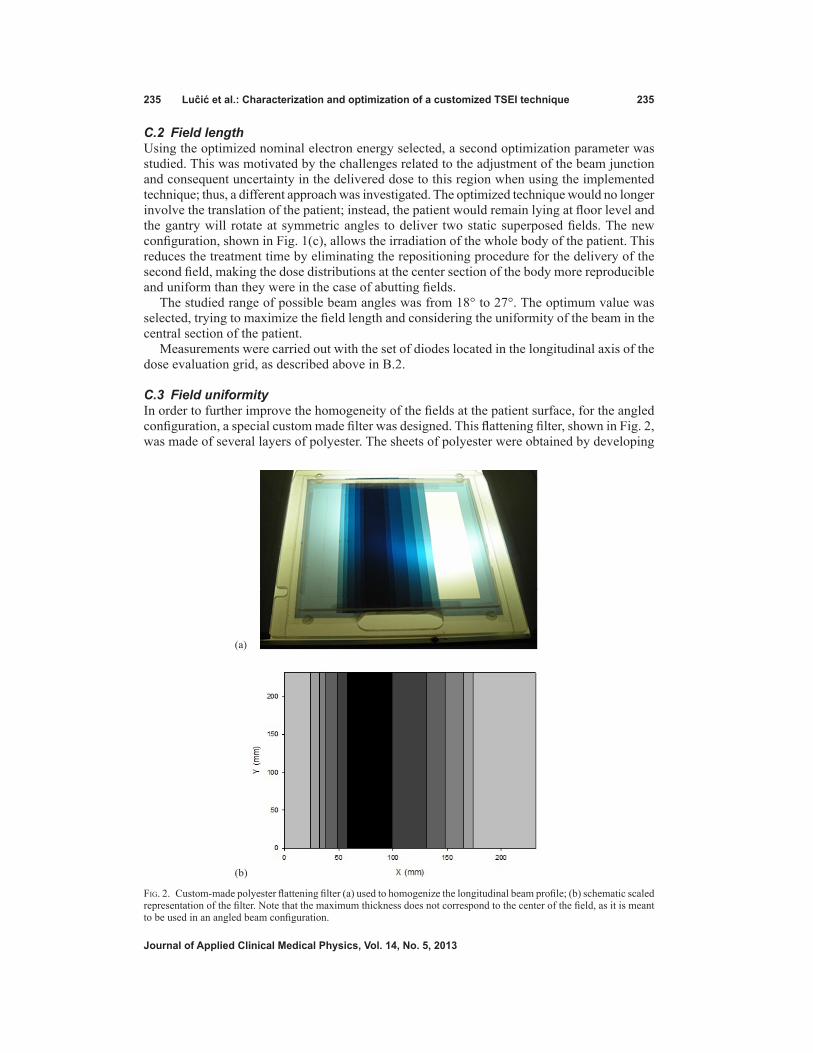
235 Luĉić et al.: Characterization and optimization of a customized TSEI technique 235
Journal of Applied clinical Medical Physics, Vol. 14, no. 5, 2013
C.2 Field length Using the optimized nominal electron energy selected, a second optimization parameter was studied. This was motivated by the challenges related to the adjustment of the beam junction and consequent uncertainty in the delivered dose to this region when using the implemented technique; thus, a different approach was investigated. The optimized technique would no longer involve the translation of the patient; instead, the patient would remain lying at floor level and the gantry will rotate at symmetric angles to deliver two static superposed fields. The new configuration, shown in Fig. 1(c), allows the irradiation of the whole body of the patient. This reduces the treatment time by eliminating the repositioning procedure for the delivery of the second field, making the dose distributions at the center section of the body more reproducible and uniform than they were in the case of abutting fields.
The studied range of possible beam angles was from 18° to 27°. The optimum value was selected, trying to maximize the field length and considering the uniformity of the beam in the central section of the patient.
Measurements were carried out with the set of diodes located in the longitudinal axis of the dose evaluation grid, as described above in B.2.
C.3 Field uniformity In order to further improve the homogeneity of the fields at the patient surface, for the angled configuration, a special custom made filter was designed. This flattening filter, shown in Fig. 2, was made of several layers of polyester. The sheets of polyester were obtained by developing
Fig. 2. Custom-made polyester flattening filter (a) used to homogenize the longitudinal beam profile; (b) schematic scaled representation of the filter. Note that the maximum thickness does not correspond to the center of the field, as it is meant to be used in an angled beam configuration.
(a)
(b)

236 Luĉić et al.: Characterization and optimization of a customized TSEI technique 236
Journal of Applied clinical Medical Physics, Vol. 14, no. 5, 2013
blank films, and were mounted in an acrylic frame. The material was selected because of its availability and its low Z value, which reduced the probability of generating bremsstrahlung. The filter was designed to be thickest at a shifted position from the geometrical center of the field, taking into consideration that the treatment was carried out by a superposition of two angled beams.
Ten diodes were used to measure the relative profile at the treatment plane of a single angled beam. The profile was back-projected to the tray plane, providing a first guess for the filter design. Then, the process was repeated, until an optimum configuration was reached. The border of the field was only slightly filtered, in order to preserve the particle fluence at the superior and inferior edges of the beam (the first sheet of polyester covered the entire exit window as a base for the additional sheets). As only one filter was build and mounted, the linac head needed to be rotated 180° for the second (symmetric) beam angle. The final configuration of the filter (sheets dimension and position) is shown in Table 1.
D. optimized techniqueAfter the optimal combination for the dual electron field was found, 2D transversal dose dis-tributions measurements were performed. This was done using film dosimetry and an anthro-pomorphic (pelvic) phantom irradiated under clinical TSEI conditions. In order to evaluate the contribution from the different beams to the final AP depth dose of the complete treatment, the phantom was irradiated using a single optimized dual beam incident from the AP direction, then from the two anterior–oblique directions, and finally from the remaining PA position, to complete the six positions described by the Stanford technique. Additionally, the previously implemented modified Stanford technique was also used to irradiate the phantom, allowing the comparison of both treatments.
III. rESuLTS
Hereon we present the results of the optimization of the TSEI treatment, comparing the char-acteristics of the optimized technique with the implemented modified Stanford technique. This is done for the single incidence dual field, as well as for the complete treatment.
A. Dual beam characteristicsTable 2 shows the result of the beam characterization under TSEI conditions (extended SSD of 200 cm) for different energies and degraders. It can be noted that, as the degrader thickness increases, the superficial dose grows, along with a decrease in R85. A slight but consistent increase in the Bremsstrahlung contamination with respect to the configuration without filter can be noted for the 8 mm filter; however, for the 12 mm filter the effect is not observed systematically.
Table 1. Characteristics of the flattening filter made of polyester.
Sheet Dimensions X Distance from the Accumulated Polyester No. X×Y (cm2) Field Edge (cm) Thickness (mm)
1 23.2×23.2 0 0.15 2 23.2×15 2.4 0.30 3 23.2×13 3.2 0.45 4 23.2×11 3.8 0.60 5 23.2×8.2 4.9 0.75 6 23.2×5 5.8 0.90 7 23.2×3.5 6.4 1.05

237 Luĉić et al.: Characterization and optimization of a customized TSEI technique 237
Journal of Applied clinical Medical Physics, Vol. 14, no. 5, 2013
The isodose curves in the transversal plane for a 9 MeV beam with an 8 mm degrader were used to evaluate the extension of the usable field (50% isodose curve). It was found that at R85 the width of the dual field was of 74 cm.
Diode measurements along the longitudinal profile for the adjacent field technique showed that the dose under the lead protection was reduced for each field to a 3.4% of the central axis dose in the case of a 6 MeV beam without filter, and to a 4.3% in the case of a 9 MeV beam filtered by the 8 mm degrader. The complete longitudinal profile was determined assuming symmetry of the distributions for the superior–inferior fields. Figure 3 shows the comparison between longitudinal profiles of the two beam settings. As can be seen, the differences remained under ± 5% for the central 180 cm of the composed field. Underdosages at the center of the dual field, with respect to the maximum dose, of 32% for the 6 MeV and of 34% for the 9 MeV (with filter) beam were found.
Considering the results shown in Table 2 and Fig. 3 and the MUs required to obtain the same detector signal at the maximum, a beam setting of 9 MeV with 8 mm degrader was chosen as the optimized energy/filter setting.
A continuous loss of uniformity in the central section of the composed field was observed for angles greater than 24°. However, for 24° the homogeneous region was very limited (100 cm long within ± 5% and 120 cm within ± 10%), dropping to only around 60% of the dose in the center at ± 90 cm from the central axis. For 27°, the central part of the field was not uniform; nevertheless, the dose at ± 90 cm from the center was close to 90% of the dose at the central axis.
The 27° angle was chosen and the additional custom-made flattening filter, described in C.3, was added to improve the uniformity in the central part of the field. The design of the added flattening filter permitted a reduction in the dose gradient with respect to the adjacent beam configuration, while increasing the dose at the borders of the central 180 cm length region by 43% with respect to the previous implementation. The comparison shown in Fig. 4, illustrates this effect.
Table 2. Beam parameters measured at 200 cm SSD for an 80 × 80 cm2 field size at the surface.
Nominal Energy (MeV) 6 9 12 15
No E0 (MeV) 5.6 8.23 10.57 13.44
acrylic Ds (%) 80.9 82.2 83.8 86.7 filter Dx (%) 0.8 1.2 1.4 1.7 R85 (mm) 18.9 28.5 36.9 47.8
8 mm E0 (MeV) 3.69 6.03 8.73 12.24
acrylic Ds (%) 91.3 88.4 89.1 90.5 filter Dx (%) 1.4 1.5 1.8 2.4 R85 (mm) 11.1 19.7 29.4 38.7
12 mm E0 (MeV) 2.98 5.58 7.87 10.65
acrylic Ds (%) 96.5 90.9 90.9 91.4
filter Dx (%) 1.4 1.2 1.3 1.6 R85 (mm) 8.4 17.5 25.9 36.1

238 Luĉić et al.: Characterization and optimization of a customized TSEI technique 238
Journal of Applied clinical Medical Physics, Vol. 14, no. 5, 2013
B. composite distributions for the optimized techniqueThe relative dose distribution obtained as a result of the superposition of the optimized beams from the six incident directions in an anthropomorphic phantom is shown in Fig. 5(a). It shows how the 85% isodose curve completely encompasses the surface of the phantom. A PDD was extracted from the film measurement and compared with the PDD obtained for the already implemented technique. Figure 5(b) shows the comparison, where the increase in the dose at the surface and photon contamination for the new technique can be noted.
Figure 6 shows depth dose curves measured at the AP axis with film dosimetry in the anthropomorphic phantom, considering the contributions of different composed fields of the optimized TSEI treatment (AP and anterior–oblique). It can be noted that the contribution to the surface dose (and down to 2 mm depth) of the superposition of AP and anterior–oblique fields triples the contribution from the AP field alone, as the contribution from the anterior–oblique fields doubles the one from the AP. When the distributions are normalized to the maximum, the PDD of the complete optimized treatment showed the expected shifting of the maximum dose toward the surface and an increase in Ds of 10%, due to the superposition of the fields, increasing the photon contamination to 4.2%.
Fig. 3. Comparison of longitudinal profiles for the adjacent field technique, normalized to 100% at the center of each field. The solid line corresponds to a 6 MeV beam without filter and the dotted line to a 9 MeV beam with 8 mm acrylic degrader. The dashed line indicates the difference.
Fig. 4. Longitudinal profiles for 9 MeV beams with the 8 mm acrylic filter measured with diodes for different delivery techniques: adjacent beams (dashed line), 27° angled beams (dotted lines), and 27° angled beams with added flattening filter (solid line).

239 Luĉić et al.: Characterization and optimization of a customized TSEI technique 239
Journal of Applied clinical Medical Physics, Vol. 14, no. 5, 2013
Fig. 5. Transversal relative dose distribution (a) obtained from a film irradiated with 6 dual fields of 9 MeV beam with degrader and added flattening filter, normalized to the dose at 12.2 mm depth along the AP axis (corresponding to R100 of the AP field); (b) composite percentage depth dose distribution for the 6 dual fields with the modified Stanford technique (dashed line) and the optimized technique (solid line).
(a)
(b)
Fig. 6. In-depth dose distributions measured at the AP axis for the contributions of: AP dual field (dashed line), anterior–oblique fields (dotted line), and the complete treatment (solid line). The planned dose was of 100 cGy at R85 for each dual field.

240 Luĉić et al.: Characterization and optimization of a customized TSEI technique 240
Journal of Applied clinical Medical Physics, Vol. 14, no. 5, 2013
c. clinical implementationOur modified Stanford technique uses a lying down positioning; this has clear advantages for weak patients. However, the application of oblique fields has challenges related to reproduc-ibility and patient comfort. In order to address this issue, pillows and foam wedges are used. Figure 7 shows the patient positioned for an anterior–oblique incidence.
As can be noted, in vivo dosimetry based on semiconductor diodes is used to monitor dose delivery, including the X-ray contamination contribution. Monitored points corresponded to the center of the field and regions of reduced diameter and/or at the borders of the treatment field (ankles, wrists, scalp, and sole of the foot). The decision of additional boosts or protection of any of these anatomical regions was made based on such measurements.
IV. DIScuSSIon & concLuSIonS
One of the objectives of this study was to find a new setting of the beam, in which the superficial dose is increased, but the therapeutic range (R85) remains as close as possible to the one from the modified Stanford technique already in use (6 MeV nominal energy without filter), limiting as much as possible the photon contamination. Considering the parameters shown in Table 2, it was found that the best compromise to fulfill these requirements was to use a 9 MeV beam either with the 8 or 12 mm degrader. However, the number of monitor units required to deliver the same dose using the 9 MeV beam with the 12 mm degrader, compared with the ones needed for the 8 mm filter, were significantly higher. Using this combination would then increase the treatment time, which would affect patient comfort, introducing more uncertainties related to patient positioning. As both techniques were able to fulfill the requirements imposed in terms of beam characteristics, but the thinner filter implied fewer MUs, the 9 MeV beam with the 8 mm filter was selected to be used in the optimized technique. This setting allowed increasing the superficial dose from 80.9% to 88.4% of the maximum, with an increase of 0.8 mm in R85, while keeping photon contamination at a low level, increasing only in a 0.9% of the maximum dose. The isodose distribution at R85 for the selected setting was considered to be appropriate for the TSEI treatment, as the width of the 50% isodose curve of 74 cm would be sufficient to cover the transversal extension of an adult patient’s thorax.
Fig. 7. Patient positioned for an anterior–oblique irradiation. Pillows and foam wedges help patient hold the position. An in vivo dosimetry system is used to monitor treatment delivery. The acrylic degrader (not seen in this picture) is placed above the patient, using the support platform and the treatment couch seen at the top and bottom of the picture, respectively.

241 Luĉić et al.: Characterization and optimization of a customized TSEI technique 241
Journal of Applied clinical Medical Physics, Vol. 14, no. 5, 2013
Although the selection of an optimized beam/filter setting produces the desired effect of increasing the dose to the surface, it does not solve the previously mentioned problems. Thus, the use of angled beams provides the ideal approach to reduce the uncertainties in the total treatment dose received by the patient at the central region. Additionally, it extends the range of the useful beam in the longitudinal direction and reduces the treatment time (by eliminating patient repositioning).
Variations in the uniformity of the beam across the longitudinal profile for the selected beam setting and different symmetric gantry angulations resulted in two expected effects. As the angle increased, a loss of uniformity in the central part of the dual field, accompanied by an increase of the field extension, was observed. Within the studied angle range, it was found that the best uniformity at the central region was achieved by the 24° angle. Under this configura-tion, the dose close to the edges of the field was reduced to 60% of the central dose. As this is considered insufficient to treat the full extension of an adult patient, a greater symmetric angle was needed to optimize the beam. Symmetric angles of 27° provided a useful field of 180 cm in the longitudinal direction, considered sufficient to treat the great majority of the patients. However, the uniformity of the dose across the field was greatly compromised by the increase in the obliquity of the beam incidence. Due to the fact that the uniformity of the beam can be further improved by the addition of a flattening filter, the 27° angle was selected regardless, prioritizing the extension of the usable beam.
The clinical beam optimized by the use of an energy of 9 MeV with a degrader, an added filter, and a symmetric rotation of the gantry in ± 27° for the subfields composing beam, allows the treatment of taller patients than it was possible with the adjacent beam technique. Furthermore, beam uniformity was improved, giving more flexibility to position the patient and reducing the treatment time. The gradient of the longitudinal profile obtained was close to the results reported by Chen et al..(11)
In Figure 5, the final transversal dose distribution obtained for the optimized TSEI treatment delivered to a phantom can be seen. Although the surface dose presents inhomogeneities (the directions of incidence are clearly noted), the 85% isodose encloses the patient’s surface in a uniform way. The increase in photon contamination (to a total of 4.2%), due to the superposi-tion of fields for the complete TSEI treatment, remains within acceptable limits recommended by the AAPM for composite electron beams.(3)
The AAPM(3) defines a B factor (overlapping factor) that can be obtained as the ratio between the mean surface dose in a cylindrical (30 cm diameter) phantom for the complete treatment, and the surface dose for a single dual field. Figure 6 shows the PDDs that allow the estimation of this factor; in this case, each composed field contributes with one third of the superficial dose. The use of factor B allows simplifying the manual treatment planning, as the dosimetry of only one field would be sufficient to estimate the dose deposition at the surface of the patient due to the contributions of the six dual fields. The factor obtained for our optimized implementation was 3, consistent with the range reported by the AAPM (from 2.5 to 3) for Stanford type TSEI techniques.(3) Due to the increase in the obliquity of the beam incidence over structures with reduced diameter (as arms and legs), an increase of the overlapping factor under these conditions would be expected for any implementation of a Stanford technique. This effect could explain short- (epithelitis) and long-term (formation of fibrotic zones and telangiectasias) unwanted reactions observed in the extremities of some patients treated at our center, and should be considered when planning the treatment.
rEFErEncES
1. Hoppe RT. Mycosis fungoides: radiation therapy. Dermatol Ther. 2003;16(4):347–54. 2. Jones GW, Racinski BM, Wilson LD, et al. Total skin electron radiation in the management of mycosis fungoides:
consensus of the European Organization for Research and Treatment of Cancer (EORTC), Cutaneous Lymphoma Project Group. J Am Acad Dermatol. 2002;47:364–70.

242 Luĉić et al.: Characterization and optimization of a customized TSEI technique 242
Journal of Applied clinical Medical Physics, Vol. 14, no. 5, 2013
3. Karzmark CJ, Anderson J, Buffa A, et al. Total skin electron therapy: technique and dosimetry. AAPM Report 23. Task Group 30 Radiation Committee. New York: American Institute of Physics; 1987.
4. Navi D, Riaz N, Levin YS, Sullivan NC, Kim YH, Hoppe RT. The Stanford University experience with conven-tional-dose, total skin electron-beam therapy in the treatment of generalized patch or plaque (T2) and tumor (T3) mycosis fungoides. Arch Dermatol. 2011;147(5):561–67.
5. Karzmark CJ, Loevinger RE, Steel RE, Weissbluth M. Technique for large-field superficial electron therapy. Radiology. 1960;74:633–44.
6. Diamantopoulos S, Platoni K, Dilvoi M, et al. Clinical implementation of total skin electron beam (TSEB) therapy: a review of the relevant literature. Phys Med. 2011;27(2):62–68.
7. Anacak Y, Arican Z, Bar-Deroma R, Tamir A, Kuten A. Total skin electron irradiation: evaluation of dose uni-formity throughout the skin surface. Med Dosim. 2003;28(1):31–34.
8. el-Khatib EG, Rymel J, al-Mokhlef J. A technique for total skin electron irradiation using six large flattened electron beams: implementation on linear accelerators having different modes of electron beam production. Br J Radiol. 1989;62(740):744–48.
9. Wu JM, Leung SW, Wang CJ, Chui CS. Lying-on position of total skin electron therapy. Int J Radiat Oncol Biol Phys. 1997;39(2):521–28.
10. IAEA. Absorbed dose determination in external beam radiotherapy: an international code of practice for dosimetry based on standards of absorbed dose to water. TRS-398. Vienna: IAEA; 2000.
11. Chen Z, Agostinelli AG, Wilson LD, Nath R. Matching the dosimetry characteristics of a dual-field Stanford technique to a customized single-field Stanford technique for total skin electron therapy. Int J Radiat Oncol Biol Phys. 2004:59(3):872–85.

a Corresponding author: Guang Li, Department of Medical Physics, Memorial Sloan-Kettering Cancer Center, 1275 York Ave., New York, NY 10065, USA; phone: (212) 639 2891; fax: (212) 717 3258; email: [email protected]
Migration from full-head mask to “open-face” mask for immobilization of patients with head and neck cancer
Guang Li,1a D. Michael Lovelock,1 James Mechalakos,1 Shyam Rao,2 Cesar Della-Biancia,1 Howard Amols,1 and Nancy Lee2 Department of Medical Physics1 and Department of Radiation Oncology,2 Memorial Sloan-Kettering Cancer Center, New York, NY, [email protected]
Received 4 February, 2013; accepted 15 May, 2013
To provide an alternative device for immobilization of the head while easing claustrophobia and improving comfort, an “open-face” thermoplastic mask was evaluated using video-based optical surface imaging (OSI) and kilovoltage (kV) X-ray radiography. A three-point thermoplastic head mask with a precut opening and reinforced strips was developed. After molding, it provided sufficient visible facial area as the region of interest for OSI. Using real-time OSI, the head motion of ten volunteers in the new mask was evaluated during mask locking and 15 minutes lying on the treatment couch. Using a nose mark with reference to room lasers, forced head movement in open-face and full-head masks (with a nose hole) was compared. Five patients with claustrophobia were immobilized with open-face masks, set up using OSI and kV, and treated in 121 fractions, in which 61 frac-tions were monitored during treatment using real-time OSI. With the open-face mask, head motion was found to be 1.0 ± 0.6 mm and 0.4° ± 0.2° in volunteers during the experiment, and 0.8 ± 0.3 mm and 0.4° ± 0.2° in patients during treat-ment. These agree with patient motion calculated from pre-/post-treatment OSI and kV data using different anatomical landmarks. In volunteers, the head shift induced by mask-locking was 2.3 ± 1.7 mm and 1.8° ± 0.6°, and the range of forced movements in the open-face and full-head masks were found to be similar. Most (80%) of the volunteers preferred the open-face mask to the full-head mask, while claustrophobic patients could only tolerate the open-face mask. The open-face mask is characterized for its immobilization capability and can immobilize patients sufficiently (< 2 mm) during radiotherapy. It provides a clinical solution to the immobilization of patients with head and neck (HN) cancer undergoing radiotherapy, and is particularly beneficial for claustrophobic patients. This new open-face mask is readily adopted in radiotherapy clinic as a superior alternative to the standard full-head mask.
PACS numbers: 87.19.xj, 87.63.L-, 87.59.-e, 87.55.tg, 87.55.-x
Key words: patient setup and immobilization, thermoplastic head mask, image-guided radiotherapy, optical surface imaging, motion uncertainty
I. IntroductIon
Historically, the widely accepted standard of care for the immobilization of patients with head and neck (HN) cancer is the thermoplastic full-head mask.(1-4) Closed-form, full-head masks have been well characterized in terms of head motion (~ 2 mm) within the mask(2,5,6) and setup uncertainty (2-3 mm),(6-9) permitting the calculation of treatment margins to account for the geometric setup uncertainty of radiotherapy. However, the full-head mask forces patients to
JournAL oF APPLIEd cLInIcAL MEdIcAL PHYSIcS, VoLuME 14, nuMBEr 5, 2013
243 243
244 Li et al.: From full-head to “open-face” mask 244
Journal of Applied clinical Medical Physics, Vol. 14, no. 5, 2013
keep the eyes and mouth closed during each daily treatment (a treatment period can last for more than 6 weeks). This is not only uncomfortable for many patients, but also intolerable for some, in particular those who suffer from claustrophobia. Although the full-head mask can be cut open around the eyes and mouth to improve patients’ comfort, mask cutting after molding is difficult, produces sharp edges, and has not been demonstrated to be helpful to claustrophobic patients. Therefore, there is a clinical demand for establishing a more practical alternative to the full-head mask to improve patient comfort and tolerability while maintaining effectiveness.
Several methods have been reported to address this clinical need. Kim et al.(10) developed a maskless technique that combines a customized head mold and a mouth-bite tray with infrared reflectors to monitor motion. It was found that the immobilization system could be tolerated by claustrophobic patients with a ~ 2 mm range of motion, but it required eight repositioning procedures, on average, during 20 treatments. The investigators also applied a partial mask to immobilize the upper face and this cut down the number of repositioning procedures to two in 20 treatments. Due to oral toxicity, the biting effort on the mouthpiece and the change in treat-ment positions, there are concerns as to whether this system could reduce patient comfort and tolerability. In a study of 260 patients, Sharp et al.(11) reported that a smaller full-head mask, in comparison with the bigger head-and-shoulder mask, reduced claustrophobic anxiety in patients significantly, together with reduced skin toxicity,(7,12) while the reproducibility of the setup and stability of the immobilization were not compromised. However, many patients still suffer from the enclosed sensation of the full-head mask.
To characterize head motion within the mask, several methods have been applied, including the comparison of X-ray images before and after treatment,(1,9) and the use of infrared reflec-tors or emitters for motion monitoring with optical sensors(13) or stereoscopic cameras.(10,14) Recently, video-based optical surface imaging (OSI) has been reported for monitoring head motion when a patient’s facial area is visible in frameless and maskless stereotactic radiosur-gery.(15,16) With a closed-form, full-head mask, this OSI method cannot be applied, since the full-head mask blocks the facial area.
From our clinical observation, despite the same head alignment strategy being applied at simulation and treatment, a head rotation often appears in setup X-ray images after the mask was placed and locked. Using open-face mask and OSI, it allows us to monitor and quantify the head positioning change during mask-locking process without ionization radiation. This piece of information is clinically useful in determining the uncertainty in patient setup, so as to the appropriate treatment margin in treatment planning.
In this study, we designed, characterized, and used an open-face mask to immobilize patients with HN cancer and claustrophobic anxiety. We first discuss a volunteer study (N = 10). Using the open-face area as the region of interest (ROI), head motion was monitored using real-time OSI motion monitoring during initial mask locking and for 15 minutes during which the vol-unteers were immobilized in the mask. The former quantifies head motion induced by mask locking for the first time, while the latter measures the absolute motion of the patient within the open-face mask. Using a marked point on the nose in reference to the room lasers, the forced movement of volunteers within both open-face and full-head masks was compared. We then discuss the application of the open-face mask in five patients with claustrophobia for treatments totaling 121 fractions. Both kilovoltage (kV) and OSI were applied for setup and assessment of patient motion. These results quantitatively characterize the immobilization performance of the open-face mask.
II. MAtErIALS And MEtHodS
A. Precut open-face mask and full-head maskThe open-face mask is a three-point (three locking points) thermoplastic head mask with a precut, isosceles-trapezoid-shaped opening, with reinforced strips around the opening and

245 Li et al.: From full-head to “open-face” mask 245
Journal of Applied clinical Medical Physics, Vol. 14, no. 5, 2013
locking edges (Orfit Industries, Wijnegem, Belgium). After molding, the opening is enlarged to show the eyes, nose, mouth, and some forehead and cheek area. The patients are unable to see the mask. The opening, as shown in Fig. 1(a), was sufficiently large to serve as the ROI (Fig. 1(d)) using the OSI real-time delta (RTD) mode for motion monitoring. The RTD mode provides three translational and three rotational motion shifts based on rapid auto-registration of the real-time images with the ROI of a reference image. The conventional three-point full-head mask has a small triangle-shaped opening, which exposes the entire nose after being molded to the patient, as shown in Fig. 1(b). The immobilization performance of the conventional mask serves as a baseline for this study.
Both open-face and conventional masks were prepared by immersion in a 65°–70°C water bath for 5 minutes. During the molding process, the warm mask was centered on the nose. The superior and inferior edges were pressed against the forehead and chin, respectively, while the lateral opening edges were pressed against the cheek, as the mask was stretched and locked on the superior and lateral sides. A similar procedure was used for the conventional mask, with the small triangle-shaped opening centered on the nose and stretched to show the entire nose. A stan-dard head support, selected to fit the individual by minimizing the gap under the neck, was used for both open-face and conventional masks. For patients, the simulation computed tomography (CT) scan was performed after the molding, whereas for volunteers, the mask was taken off after 10 minutes of cooling. All masks were used after 24 hours for the experiment or treatment.
B. optical surface imaging and kilovoltage X-ray imagingA clinical OSI (AlignRT; VisionRT, London, UK) was used in this study. It contained three ceiling-mounted stereoscopic camera pods in the treatment room of a linear accelerator (Trilogy; Varian Medical Systems, Palo Alto, CA), as shown in Fig. 2. The system was calibrated monthly and verified daily, using a calibration plate, which was placed at the machine isocenter. This
Fig. 1. An open-face mask and a conventional full-head mask molded on two volunteers. An arbitrary alignment point was marked on the masks. For the open-face mask (a), the open area was set to be the region of interest for AlignRT motion monitoring. For the conventional mask (b), the nose area was open, allowing alignment between a skin mark and the room laser in a forced motion test. A raw reference image (c), where the open area is clearly seen; the ROI (d) drawn on the reference image.

246 Li et al.: From full-head to “open-face” mask 246
Journal of Applied clinical Medical Physics, Vol. 14, no. 5, 2013
system had two acquisition modes: static image capture (SIC) to acquire one image with high resolution, and RTD to continuously capture a series of images at a lower resolution. The frame rate was 2 to 3 frames per second (fps) in RTD mode, including image registration to the ROI at the mask opening. The ROI defined on CT-based external contours was used for setup, whereas the ROI defined on an on-site reference SIC image was used for RTD motion monitoring. In addition to RTD motion monitoring, head motion was also estimated based on pre- and post-treatment SIC, using both CT-based reference and on-site SIC reference. When an on-site SIC image was captured as the reference image, the accuracy of motion monitoring has 0.2 mm accuracy(15,16) for head motion detection.
Using an on-board imager (OBI; Varian Medical Systems, Palo Alto, CA), kV X-ray imaging (orthogonal pair) was acquired for daily patient setup. Image registration was based on bony landmarks. The patient motion extracted from pre- and post-treatment images was compared with the corresponding OSI data (SIC and RTD) for conformation using different anatomical landmarks. All 2D kV image registrations on bony landmarks were performed by therapists manually and verified by a physicist.
c. Volunteers and patient selectionTen volunteers (six male and four female) were accrued from employee workers in the Memorial Hospital. Both open-face and full-head masks were molded with a head support selected for each volunteer. An arbitrary isocenter was chosen and marked on the masks.
Five patients (three male and two female) who could not tolerate the conventional mask were selected to use the open-face mask for immobilization during their simulation and multi-fractionated treatment. Patients were simulated in a positron emission tomography (PET)/CT scanner (Discovery; GE Healthcare, Milwaukee, WI) for treatment planning. The disease sites were close to the facial area; they included the parotid, ear, neck, nasal skin, and base of tongue. For the patient with a disease site on the nasal skin, a bolus was taped on the skin in the opening area of the mask during his hypofractional treatment. The bolus and the rest of the opening surface were used as the ROI for RTD motion monitoring for this patient, after initial setup with the skin ROI in the opening area of his mask. Patient’s Karnofsky performance status (KPS) ranged from 80 to 100.
Fig. 2. A video-based optical surface imaging system (AlignRT) with three ceiling-mounted stereoscopic camera pods in a treatment room with a linear accelerator (Trilogy).

247 Li et al.: From full-head to “open-face” mask 247
Journal of Applied clinical Medical Physics, Vol. 14, no. 5, 2013
d. Experimental procedure for volunteers Three experiments were performed to measure the following three motions for each volunteer: (1) mask-locking–induced head shifts; (2) head motion during 15 minutes of immobilization in the open-face mask; and (3) forced movement inside both mask types.
Mask-locking–induced head motion using RTD: Each of the volunteers was aligned on the longitudinal midline along the nose and chin to the sagittal room laser, and on the tragus to the transverse (vertical) and coronal (horizontal) lasers. The open-face mask was then loosely laid on the subject’s face. A reference SIC image was acquired to serve as ideal setup position (since there is no CT image for volunteers) before each RTD acquisition during mask locking. The volunteers were informed that they should retain the head position and orientation despite the fact that they may sense their head being dragged away during mask locking. The procedure was repeated three times.
Head motion during 15-minute immobilization: All volunteers were instructed to lie still for 15 minutes after a SIC image was captured as the reference for RTD.
Forced movement under the masks: A dot was drawn with a marker pen on the tip of the subject’s nose at the cross point of the sagittal and transverse lasers. The volunteer was instructed to move forcefully to the left and right, and to move chin up, and chin down. Using a ruler with an accuracy of 1.0 mm, the displacement between the skin mark and the laser line was measured, and three replicates were recorded in each direction. The absolute motions for left and right directions were averaged together, while chin-up and chin-down were averaged together. An example of RTD data for a volunteer with the open-face mask is shown in Fig. 3. The absolute amplitudes of the motion in all four directions were calculated in both open-face and full-head masks for comparison.
Fig. 3. Demonstration of the forced motion in four directions of a volunteer subject wearing the open-face mask. The colored lines are movements in vertical (D.VRT), longitudinal (D.LNG), and lateral (D.LAT) directions or rotational axes. The gray line is the motion amplitude. Note that after a forced motion, the subject’s position tends to fall back to within 1.5 mm of its original baseline.

248 Li et al.: From full-head to “open-face” mask 248
Journal of Applied clinical Medical Physics, Vol. 14, no. 5, 2013
E. clinical procedure for patientsAll five patients were set up initially with OSI guidance. If the rotation of the head was found to be greater than 2° in any direction, the mask was unlocked, the patient was adjusted, and the mask was locked again to attempt to correct the head rotation. An orthogonal kV image pair was used for final setup. A SIC image was acquired after setup to serve as the reference for RTD and as the pretreatment OSI image. At the end of each treatment, both kV imaging and OSI were repeated to evaluate patient motions. This procedure was performed for all 121 fractions of treatment for the patients, except for RTD, which was performed in only 61 frac-tions. The RTD data were acquired throughout the entire treatment. Previously, a baseline drift was found in RTD acquisition due to possible thermal effect of the OSI system (0.5 mm drift in the vertical direction during the first 5–10 minutes), likely caused by the heat released from the central speckle projector.(16) This drift was corrected by subtracting the baseline from RTD measurement curves.
III. rESuLtS
A. Mask-locking–induced head shift in open-face maskTable 1 shows the RTD data during the initial mask locking process. On average, mask lock-ing induces a head shift of 2.3 ± 1.7 mm and 1.8° ± 0.6°. It is interesting to note that the first locking almost always induces a higher head shift, and the shift levels off in the second and third locking trials. This result suggests that if a large shift of the head was induced in the first locking, a second trial is worthwhile to reduce it. In fact, we tried to correct head rotation in patients, if it was greater than 2°, with a second trial.
Table 1. Change in the head position of ten volunteers during the mask-locking process using the open-face mask and AlignRT motion monitoring. Three trials for each subject were performed. The first mask locking almost always caused greater head motion than the second and third trials. On average, a second trial in setup could reduce mask-locking–induced head shifts by 1 mm and 1°.
Volunteer Translation (mm) Rotation (°) Subject Trial 1 Trial 2 Trial 3 Mean Trial 1 Trial 2 Trial 3 Mean
1 0.1 0.3 0.9 0.4 1.9 1.9 1.5 1.8 2 4.5 1.8 2.2 2.8 4.0 1.9 1.8 2.6 3 3.5 2.9 3.0 3.2 1.6 0.8 0.8 1.0 4 3.0 2.0 1.2 2.1 2.5 1.3 2.6 2.1 5 2.6 0.5 0.5 1.2 3.0 1.4 2.0 2.1 6 2.2 0.5 1.0 1.2 2.1 0.8 1.4 1.4 7 4.3 3.1 2.6 3.3 1.3 1.4 1.2 1.3 8 1.4 1.2 0.3 1.0 1.0 1.3 0.8 1.0 9 9.9 4.6 4.3 6.3 4.2 1.8 2.1 2.7 10 2.2 1.9 1.4 1.9 3.1 1.0 1.2 1.8 Average 3.4 1.9 1.8 2.3 2.5 1.4 1.5 1.8 St dev 2.7 1.4 1.3 1.7 1.1 0.4 0.6 0.6

249 Li et al.: From full-head to “open-face” mask 249
Journal of Applied clinical Medical Physics, Vol. 14, no. 5, 2013
B. comparison of forced movement in open-face and full-head masksTable 2 shows the comparison of the forced (translational) movement of ten volunteers in both masks. On average, the open-face mask allows a maximum movement (from left or right and chin up or chin down actions) of 5.5 ± 2.5 mm (lateral) and 4.2 ± 2.0 mm (longitudinal). Eight out of ten subjects in this study preferred the open-face mask to the full-head mask, based on their comfort level during the experiment. Figure 3 shows RTD motion curves (3–4 replicates for each direction) in six degrees of freedom, including rotational shifts. Also note that for chin-up and chin-down moves, vertical position was also changed, but not recorded in Table 2. This RTD test cannot be performed for the full-head mask, as the nasal surface is too small to produce any reliable result. An important phenomenon observed in all volunteers is that no matter how the forced motion occurs, when the force is released, the head will fall back to its original position within 1 to 2 mm, as shown in Fig. 3.
c. Head immobilization and stability using open-face maskFigure 4 shows the motion of the heads of ten volunteers in the open-face mask, which averaged 1.0 ± 0.6 mm and 0.4° ± 0.4°. During the 15 minutes of immobilization, the volunteers blinked
Table 2. Comparison of the forced motion of volunteers wearing the open-face mask or conventional full-head mask. Six measurements (three in each direction) were performed to calculate the mean motion using a skin marker against the room laser reference. On average, the open-face mask allowed a larger maximum shift than the conventional mask by 1 mm. This was because the edges of the nose opening in the conventional mask caused the volunteers discomfort when they were asked to move in some directions.
Left or Right (mm) Chin Up or Down (mm) Open-face mask Full-head mask Open-face mask Full-head mask Preference Volunteer Mean St dev Mean St dev Mean St dev Mean St dev (OF vs. FH)
1 7.3 0.5 6.3 1.2 7.3 1.5 6.3 3.0 OF 2 2.8 0.4 2.7 0.8 1.9 1.0 2.0 0.0 OF 3 2.6 0.5 1.9 0.2 2.3 0.4 2.3 0.5 OF 4 7.9 0.7 2.9 0.7 6.2 0.8 3.7 0.5 OF 5 7.9 1.5 4.0 1.1 5.3 3.3 2.0 0.0 OF 6 7.6 1.6 3.5 1.2 4.2 0.8 3.3 1.5 FH 7 3.3 0.5 1.0 0.0 3.7 0.5 2.8 0.8 OF 8 2.3 1.1 1.7 0.5 1.8 0.8 1.8 0.4 OF 9 8.1 1.3 8.8 1.0 6.5 0.6 3.0 0.6 FH 10 5.0 1.9 9.5 1.4 2.7 1.4 5.2 2.3 OF Average 5.5 1.0 4.2 0.8 4.2 1.1 3.3 1.0 8OF vs. 2FH St dev 2.5 3.0 2.0 1.5
OF = open-face mask; FH = full-head mask.
Fig. 4. Translational and rotational motion (vector) average with standard deviation (error bar) in 15 minutes for ten volunteers. The mean is 1.0 ± 0.6 mm and 0.4° ± 0.4°.

250 Li et al.: From full-head to “open-face” mask 250
Journal of Applied clinical Medical Physics, Vol. 14, no. 5, 2013
their eyes frequently, but this had no noticeable effect (< 1 mm) on the motion of their heads. Figure 5 shows the RTD data from four patients during 57 fractions of treatment. The average motion was found to be 0.8 ± 0.3 mm and 0.4° ± 0.2°. This is in a close agreement with the volunteer data discussed above. It is interesting to note that although the mask becomes loose in later fractions, head motion remains around the same level.
Fig. 5. The head motion (vector) of four patients during radiation treatment in 11 to 16 fractions per patient. The mean for all patients and fractions is 1.5 mm and 0.5°, which is consistent with the volunteer data shown in Fig. 4. Although patient weight loss was observed as the mask fit more loosely in later fractions, no significant increase in motion was observed. The linear regression fit (dotted line) is shown in each graph. In the first 2 patients, the shift difference between before and after (B&A) SIC images is provided.

251 Li et al.: From full-head to “open-face” mask 251
Journal of Applied clinical Medical Physics, Vol. 14, no. 5, 2013
D. Confirmation of intrafractional motion with pre-/post-treatment kV and OSI dataTable 3 shows the comparison between the patients’ RTD and pre- and post-treatment SIC data using OSI. The translational data from pre- and post-treatment kV is also included. The RTD data are in close agreement with the OSI results using the on-site ROI as the reference image, but differs from OSI results using the CT-based ROI as the reference image, mostly due to the rotational difference between the simulation position and treatment position. The kV data fall in between OSI-1 and OSI-2, since the alignment of kV images tends to compromise among different bony landmarks in the presence of head rotation.
IV. dIScuSSIon
A. Absolute head motion inside open-face maskIn this study, we measured head stability in 15 human subjects inside the open-face mask during 15 minutes or more using RTD. Head stability was confirmed by kV X-ray imaging in patients, providing direct and quantitative results on the quality of the new open-face mask in the clinic. This RTD measurement cannot be conducted with the conventional enclosed full-head mask, since the ROI on the nose is insufficient for monitoring. The ROI, which is defined as the entire opening area of the mask (Fig. 1), covers most of the central face area, which was reported useful for phantom and patient setup,(17) although a smaller ROI tends to result in nosier registration results. Previously, surface or marker imaging over the mask itself has been reported as a surrogate for patient motion,(18,19) but we consider direct imaging of the skin more accurate and reliable. For instance, if full-head mask becomes lose, then small head motion within the conventional mask may not be detectable. Furthermore, the uneven surface of the mask introduces uncertainty in surface imaging and registration. In this study, although relative comparison of the full-head mask is limited to only point-checking in forced movement, the information on absolute motion for the open-face mask, together with setup uncertainty, is useful in the determination of treatment margins for this immobilization method.
From the forced movement experiment, it is interesting to see that, although the reinforcing strips in the open-face mask (Fig. 1) makes it sturdier than the conventional mask, subjects can move slightly more in the open-face masks than in the full-head masks. In the conventional mask, the presence of the sharp edge around the nose opening limits further movement when it touches the nose. According to the manufacturer (Orfit Industries), the strength of the two
Table 3. Head motion of five claustrophobic patients monitored with AlignRT in real time during treatment, and with both AlignRT and orthogonal kV imaging in pre- and post-treatment (P&P). The average motion of these patients is similar to that of the volunteers. The X-ray P&P data fall between two sets of AlignRT P&P data (OSI-1 and OSI-2) using different reference images. Note: both OSI-1 and OSI-2 show P&P differences, quantifying head motion during treatment, although OSI-1 is more reliable since it does not carry residual head rotation at setup.
Translation (mm) Rotation (degree) RTD P&P X-ray RTD P&P Patient Sex Age fx/Fxa Mean St dev OSI-1b OSI-2c kV Mean St dev OSI-1 OSI-2
1 M 65 16/30 1.2 0.6 1.3 2.3 1.7 0.5 0.2 0.6 1.1 2 F 72 11/20 0.7 0.1 0.9 1.5 1.0 0.3 0.1 0.3 1.2 3 M 59 16/33 0.6 0.3 0.5 1.4 1.2 0.3 0.1 0.2 0.6 4 M 76 4/5 0.5 0.2 1.3 1.0 1.1 0.6 0.2 0.8 0.2 5 F 55 14/33 0.9 0.4 1.1 1.6 1.4 0.4 0.2 0.4 0.8 Average 65 12/24 0.8 0.3 1.0 1.6 1.4 0.4 0.2 0.5 0.8 St dev 0.3 0.4 0.5 0.5 0.2 0.3 0.4
a fx/Fx refers to the number of fractions (fx) for which AlignRT was applied for motion monitoring over the total number of treatment fractions (Fx).
b OSI-1 uses the on-site AlignRT image as the registration reference image, for pre- and post-treatment registration.c OSI-2 uses the CT external contours as the registration reference image, for pre- and post-treatment registration.

252 Li et al.: From full-head to “open-face” mask 252
Journal of Applied clinical Medical Physics, Vol. 14, no. 5, 2013
masks in resistance to an external horizontal force is almost identical in their head phantom tests. This is consistent with our finding in this study: the maximum range of the voluntary motion for both masks is similar, around 10 mm. On the other hand, the immobilization device is designed primarily to prevent involuntary head motion, which is much smaller in scale, as shown in Table 3, Fig. 4, and Fig. 5. Clinically, the forced movements rarely happen, but the experiment provides the limits on extreme head movements (as shown in Table 2) and likeli-hood of settling back to the original position after relaxation (as shown in Fig. 3). The gating function of AlignRT in RTD mode can be used to turn the treatment beam off, in case patients did move substantially within the open-face mask. In contrast, this real-time imaging option is not available for full-head mask. Although a mouth-bite infrared reflector array could be used for optical motion tracking, this method is not ideal for HN cancer patients due to potential oral toxicity.
In comparison with previously published data on the full-head mask,(2,5,6) our data on head motion inside the open-face mask show consistent results for both volunteers and patients. Any involuntary head motion is restricted to within 2 mm at 95% confidence level. Note that the average age is around 35 for volunteers and 65 for patients. In addition, because of the facial opening in the mask, we can also evaluate the shift in head position induced by mask-locking. This observation provides direct quantified evidence of mask-locking–induced head motion for the first time, and further evaluation may be needed, including additional evaluation on different days and by different users. One outlier with ~ 1 cm dragged distance could have resulted from several factors: the female subject’s hair got in the way of the locking slot, her mask appeared to be extremely tight, and she did not apply enough counter-dragging force to retain head position. More importantly, the result derived from the open-face mask could apply to the full-head mask where real-time motion detection on patient skin is not possible. Our study has shown that this open-face mask can be used in routine radiotherapy, providing immobilization within 2.0 mm, with improved patient comfort and tolerability.
B. General concerns for patient comfortThis study has demonstrated that some patients, who suffer from claustrophobic anxiety and cannot tolerate the conventional full-head mask, can, in fact, tolerate the open-face mask. This suggests that the open-face mask can be applied with a larger population of patients with improved comfort. It has been reported that patients who are covered less experience less claustrophobic distress while being immobilized. Sharp et al.(11) reported that use of a smaller three-point full-head mask reduced claustrophobic feelings and skin toxicity, in comparison with a larger five-point head-and-shoulder mask, while similar patient immobilization was retained. Kim et al.(10) reported that an upper-face mask without chin restriction can ease patient claustrophobic anxiety, while a mouth-bite tray can be used to place infrared reflectors to monitor head motion. Severely claustrophobic patients, however, may not be able to tolerate the open-face mask. In this case, daily prior-treatment medication, including anesthesia, may have to be used for the entire treatment period. With mild or moderate claustrophobic patients, the open-face mask has performed well in our radiotherapy clinic.
We surveyed the volunteers about the level of comfort they experienced in both masks immediately after they wore them in the experiment. Eight out of the ten volunteers preferred the open-face mask. With the full-head mask, subjects are forced to keep their eyes and mouth closed, leaving them in the “dark” during the 20-minute treatment everyday for six weeks. The open-face mask removes this restriction. This advantage, along with those discussed above, makes the use of the open-face mask favorable over the conventional full-head mask in the clinic.
c. other clinical considerationsIt is also worthwhile to note that the size of the facial opening is critical to both the quality of immobilization and visualization of OSI (SIC and RTD). There is a tradeoff between them,

253 Li et al.: From full-head to “open-face” mask 253
Journal of Applied clinical Medical Physics, Vol. 14, no. 5, 2013
and we found that the size of the opening of the open-face mask can achieve clinically accept-able levels for both immobilization and surface imaging. We consider that the ROI meets the minimal requirement for an accurate and reliable registration for setup and motion monitoring. Because of the small ROI at the opening (Fig. 1(d)), a change in facial expression, such as smiling or squeezing the nose, could cause an apparent shift in RTD signal or a false positive. However, a patient on treatment is unlikely to have these facial expressions, and even if they do, the motion signal will fall back to the original level after the patient has relaxed. For other minor facial expressions, such as blinking, we found that they did not cause a noticeable change (< 1 mm) in RTD motion monitoring.
Due to the opening in the open-face mask, the cast line on the mask may not form a cross point for setup. Therefore, the alignment of the patient with the room lasers has to rely on an incomplete line. In some cases, the open-face mask could be twisted during the six-week treat-ment course, resulting in two partial lines that no longer align with the laser line. This could result from changes in patient anatomy during the course of treatment, as we have observed the looseness of the mask in later fractions. In this case, we recommend that the difference is split for conventional setup.
We are currently investigating the accuracy of patient setup using daily kV imaging and comparing the open-face and full-head masks in patients. The collection of setup 2D kV images from two cohorts of patients is completed and analyzed: one with open-face masks and the other with full-head masks, aiming to make a direct comparison of the two masks. A followup report is expected on using different bony landmarks for registration between 2D kV and digitally reconstructed radiograph of planning CT for setup evaluation and between pre- and post-treatment 2D kV images for motion assessment.
We have used OSI to quantify head motion during 15–20 minute period for both volunteers and HN patients with open-face mask. On HN patients, the motion range was confirmed with pre- and post-treatment 2D kV and OSI static imaging. The absolute motion range was measured to assess motion uncertainty, which can be incorporated in the margin for planning tumor volume using this immobilization system. In addition, mask-locking–induced motion was measured using real-time OSI, and further investigation is worthwhile to assess this uncertainty system-atically for conventional patient setup. Although a large head movement rarely occurs during treatment, once it happens as simulated in forced movement experiments, upon relaxation the head almost always settles back to its original position within 2 mm.
V. concLuSIonS
We have established and characterized a new precut open-face thermoplastic mask for immo-bilization of patients with head and neck, cervical spine, and brain cancer during radiotherapy. Using real-time OSI, absolute head motion during 15 minutes or more on the treatment couch was found to be approximately 1.0 ± 0.5 mm for both healthy volunteers and patients with claustrophobia. Mask-locking–induced head shifts and rotations were quantified and accounted for as the uncertainty in conventional setup. The open-face mask opening (with reinforced strips) does not reduce the strength of the mask, in comparison with the full-head mask. The new open-face mask improves comfort and tolerability for patients, particularly those with moderate claustrophobic anxiety, and can be readily applied in clinical practice.
AcknowLEdGMEntS
The authors thank Mr. Marty Ratner (Orfit Industries) and Dr. Norman Smith (VisionRT Inc.) for their cooperation and for manufacturing the designed open-face masks for this clinical study. We sincerely thank all participating therapists at CT simulation and treatment (R443),
254 Li et al.: From full-head to “open-face” mask 254
Journal of Applied clinical Medical Physics, Vol. 14, no. 5, 2013
especially Ms. Marcia Chong Ton and Ms. Laura Boone, for their participation and dedication to high-quality patient care. Finally, we are grateful to all the volunteers in this study, including ZS, RK, BS, SR, ML, YL, FL, LF, JT, and KE. We appreciate the comments from the peer-review process, which have invoked improvements for this manuscript.
rEFErEncES
1. Verhey LJ, Goitein M, McNulty P, Munzenrider JE, Suit HD. Precise positioning of patients for radiation therapy. Int J Radiat Oncol Biol Phys. 1982;8(2):289–94.
2. Thornton AF, Jr., Ten Haken RK, Gerhardsson A, Correll M. Three-dimensional motion analysis of an improved head immobilization system for simulation, CT, MRI, and PET imaging. Radiother Oncol. 1991;20(4):224–28.
3. Willner J, Flentje M, Bratengeier K. CT simulation in stereotactic brain radiotherapy – analysis of isocenter reproducibility with mask fixation. Radiother Oncol. 1997;45(1):83–88.
4. Gilbeau L, Octave-Prignot M, Loncol T, Renard L, Scalliet P, Gregoire V. Comparison of setup accuracy of three different thermoplastic masks for the treatment of brain and head and neck tumors. Radiother Oncol. 2001;58(2):155–62.
5. Tsai JS, Engler MJ, Ling MN, et al. A non-invasive immobilization system and related quality assurance for dynamic intensity modulated radiation therapy of intracranial and head and neck disease. Int J Radiat Oncol Biol Phys. 1999;43(2):455–67.
6. Tryggestad E, Christian M, Ford E, et al. Inter- and intrafraction patient positioning uncertainties for intracranial radiotherapy: a study of four frameless, thermoplastic mask-based immobilization strategies using daily cone-beam CT. Int J Radiat Oncol Biol Phys. 2011;80(1):281–90.
7. Velec M, Waldron JN, O’Sullivan B, et al. Cone-beam CT assessment of interfraction and intrafraction setup error of two head-and-neck cancer thermoplastic masks. Int J Radiat Oncol Biol Phys. 2010;76(3):949–55.
8. Kang H, Lovelock DM, Yorke ED, Kriminski S, Lee N, Amols HI. Accurate positioning for head and neck cancer patients using 2D and 3D image guidance. J Appl Clin Med Phys. 2011;12(1):3270.
9. Ohtakara K, Hayashi S, Tanaka H, et al. Clinical comparison of positional accuracy and stability between dedicated versus conventional masks for immobilization in cranial stereotactic radiotherapy using 6-degree-of-freedom image guidance system-integrated platform. Radiother Oncol. 2012;102(2):198–205.
10. Kim S, Akpati HC, Li JG, Liu CR, Amdur RJ, Palta JR. An immobilization system for claustrophobic patients in head-and-neck intensity-modulated radiation therapy. Int J Radiat Oncol Biol Phys. 2004;59(5):1531–39.
11. Sharp L, Lewin F, Johansson H, Payne D, Gerhardsson A, Rufgvist LE. Randomized trial on two types of ther-moplastic masks for patient immobilization during radiation therapy for head-and-neck cancer. Int J Radiat Oncol Biol Phys. 2005;61(1):250–56.
12. Lee N, Chuang C, Quivey JM, et al. Skin toxicity due to intensity-modulated radiotherapy for head-and-neck carcinoma. Int J Radiat Oncol Biol Phys. 2002;53(3):630–37.
13. Schulte RW, Fargo RA, Meinass HJ, Slater JD, Slater JM. Analysis of head motion prior to and during proton beam therapy. Int J Radiat Oncol Biol Phys. 2000;47(4):1105–10.
14. Ryken TC, Meeks SL, Pennington EC, et al. Initial clinical experience with frameless stereotactic radiosurgery: analysis of accuracy and feasibility. Int J Radiat Oncol Biol Phys. 2001;51(4):1152–58.
15. Cervino LI, Pawlicki T, Lawson JD, Jiang SB. Frame-less and mask-less cranial stereotactic radiosurgery: a feasibility study. Phys Med Biol. 2010;55(7):1863–73.
16. Li G, Ballangrud A, Kuo LC, et al. Motion monitoring for cranial frameless stereotactic radiosurgery using video-based three-dimensional optical surface imaging. Med Phys. 2011;38(7):3981–94.
17. Peng JL, Kahler D, Li JG, et al. Characterization of a real-time surface image-guided stereotactic positioning system. Med Phys. 2010;37(10):5421–33.
18. Li S, Liu D, Yin G, Zhuang P, Geng J. Real-time 3D-surface-guided head refixation useful for fractionated stereotactic radiotherapy. Med Phys. 2006;33(2):492–503.
19. Linthout N, Verellen D, Tournel K, Storme G. Six dimensional analysis with daily stereoscopic x-ray imag-ing of intrafraction patient motion in head and neck treatments using five points fixation masks. Med Phys. 2006;33(2):504–13.

a Corresponding author: Mitsuhiro Nakamura, Department of Radiation Oncology and Image-applied Therapy, Graduate School of Medicine, Kyoto University, 54 Shogoin-Kawaharacho, Sakyo-ku, Kyoto, 606-8507, Japan; phone: ;81-75-751-3762; fax: +81-75-771-9749; email: [email protected]
Effect of audio instruction on tracking errors using a four-dimensional image-guided radiotherapy system
Mitsuhiro Nakamura,1a Akira Sawada,2 Nobutaka Mukumoto,1 Kunio Takahashi,3 Takashi Mizowaki,1 Masaki Kokubo,4,5 Masahiro Hiraoka1
Department of Radiation Oncology and Image-applied Therapy,1 Graduate School of Medicine, Kyoto University, Kyoto, Japan; Department of Radiological Technology,2 Faculty of Medical Science, Kyoto College of Medical Science, Kyoto, Japan; Advanced Mechanical Systems Department,3 Mitsubishi Heavy Industries Ltd., Hiroshima, Japan; Department of Radiation Oncology,4 Kobe City Medical Center General Hospital, Hyogo, Japan; Division of Radiation Oncology,5 Institute of Biomedical Research and Innovation, Hyogo, [email protected]
Received 17 April, 2013; accepted 10 June, 2013
The Vero4DRT (MHI-TM2000) is capable of performing X-ray image-based tracking (X-ray Tracking) that directly tracks the target or fiducial markers under continuous kV X-ray imaging. Previously, we have shown that irregular respiratory patterns increased X-ray Tracking errors. Thus, we assumed that audio instruction, which generally improves the periodicity of respiration, should reduce tracking errors. The purpose of this study was to assess the effect of audio instruction on X-ray Tracking errors. Anterior–posterior abdominal skin-surface displacements obtained from ten lung cancer patients under free breathing and simple audio instruction were used as an alternative to tumor motion in the superior–inferior direction. First, a sequential predictive model based on the Levinson–Durbin algorithm was created to estimate the future three-dimensional (3D) target position under continuous kV X-ray imaging while moving a steel ball target of 9.5 mm in diameter. After creating the predictive model, the future 3D target position was sequentially calculated from the current and past 3D target positions based on the predictive model every 70 ms under continuous kV X-ray imaging. Simultaneously, the system controller of the Vero4DRT calculated the corresponding pan and tilt rotational angles of the gimbaled X-ray head, which then adjusted its orientation to the target. The calculated and current rotational angles of the gimbaled X-ray head were recorded every 5 ms. The target position measured by the laser displacement gauge was synchronously recorded every 10 msec. Total tracking system errors (ET) were compared between free breathing and audio instruction. Audio instruc-tion significantly improved breathing regularity (p < 0.01). The mean ± standard deviation of the 95th percentile of ET (E95
T ) was 1.7 ± 0.5 mm (range: 1.1–2.6 mm) under free breathing (E95
T,FB) and 1.9 ± 0.5 mm (range: 1.2–2.7 mm) under audio instruction (E95
T,AI). E95T,AI was larger than E95
T,FB for five patients; no sig-nificant difference was found between E95
T,FB and E95T,AI (p = 0.21). Correlation
analysis revealed that the rapid respiratory velocity significantly increased E95T .
Although audio instruction improved breathing regularity, it also increased the respiratory velocity, which did not necessarily reduce tracking errors.
PACS number: 87.55.ne, 87.57.N-, 87.59.C-,
Key words: Vero4DRT, dynamic tumor tracking, tracking accuracy, audio instruction, respiration, phantom study
JOURNAL OF APPLIED CLINICAL MEDICAL PHYSICS, VOLUME 14, NUMBER 5, 2013
255 255
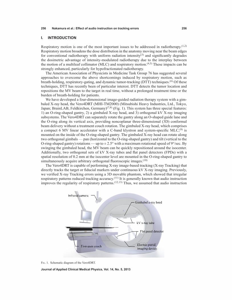
256 Nakamura et al.: Effect of audio instruction on tracking errors 256
Journal of Applied Clinical Medical Physics, Vol. 14, No. 5, 2013
I. INtRODUCtION
Respiratory motion is one of the most important issues to be addressed in radiotherapy.(1,2) Respiratory motion broadens the dose distribution in the anatomy moving near the beam edges for conventional radiotherapy with uniform radiation intensity(3) and significantly degrades the dosimetric advantage of intensity-modulated radiotherapy due to the interplay between the motion of a multileaf collimator (MLC) and respiratory motion.(4,5) These impacts can be strongly enhanced, particularly for hypofractionated radiotherapy.
The American Association of Physicists in Medicine Task Group 76 has suggested several approaches to overcome the above shortcomings induced by respiratory motion, such as breath-holding, respiratory-gating, and dynamic tumor-tracking (DTT) techniques.(6) Of these techniques, DTT has recently been of particular interest. DTT detects the tumor location and repositions the MV beam to the target in real time, without a prolonged treatment time or the burden of breath-holding for patients.
We have developed a four-dimensional image-guided radiation therapy system with a gim-baled X-ray head, the Vero4DRT (MHI-TM2000) (Mitsubishi Heavy Industries, Ltd., Tokyo, Japan; BrainLAB, Feldkirchen, Germany)(7,8) (Fig. 1). This system has three special features: 1) an O-ring-shaped gantry, 2) a gimbaled X-ray head, and 3) orthogonal kV X-ray imaging subsystems. The Vero4DRT can separately rotate the gantry along an O-shaped guide lane and the O-ring along its vertical axis, providing noncoplanar three-dimensional (3D) conformal beam delivery without a treatment couch rotation. The gimbaled X-ray head, which comprises a compact 6 MV linear accelerator with a C-band klystron and system-specific MLC,(9) is mounted on the inside of the O-ring-shaped gantry. The gimbaled X-ray head can rotate along two orthogonal gimbals — pan (horizontal to the O-ring-shaped gantry) and tilt (vertical to the O-ring-shaped gantry) rotations — up to ± 2.5° with a maximum rotational speed of 9°/sec. By swinging the gimbaled head, the MV beam can be quickly repositioned around the isocenter. Additionally, two orthogonal sets of kV X-ray tubes and flat panel detectors (FPDs) with a spatial resolution of 0.2 mm at the isocenter level are mounted in the O-ring-shaped gantry to simultaneously acquire arbitrary orthogonal fluoroscopic images.(10)
The Vero4DRT is capable of performing X-ray image-based tracking (X-ray Tracking) that directly tracks the target or fiducial markers under continuous kV X-ray imaging. Previously, we verified X-ray Tracking errors using a 3D movable phantom, which showed that irregular respiratory patterns reduced tracking accuracy.(11) It is generally known that audio instruction improves the regularity of respiratory patterns.(12,13) Thus, we assumed that audio instruction
Fig. 1. Schematic diagram of the Vero4DRT.

257 Nakamura et al.: Effect of audio instruction on tracking errors 257
Journal of Applied Clinical Medical Physics, Vol. 14, No. 5, 2013
would improve tracking accuracy. The purpose of the present study was to assess the effect of audio instruction on X-ray Tracking errors of the Vero4DRT.
II. MAtERIALS AND MEtHODS
A. Respiratory motion dataAnterior–posterior (AP) abdominal skin-surface displacements obtained from ten lung cancer patients under free breathing and simple audio instruction were used as an alternative to tumor motion in the superior–inferior (SI) direction. Under audio instruction, all patients were asked to breathe by following the simple audio instruction only, such as “breathe in, breathe out”, at a suitable tempo for each patient.(13) Table 1 shows the peak-to-peak motion amplitude (A) and the breathing period (T) of the respiratory pattern for each patient, under free breathing and under audio instruction. The coefficient of variation (CV), defined as the radio of the standard deviation (SD) to the mean, was used to evaluate the regularity of breathing patterns.
B. Experimental systemOur experimental system comprised a 3D movable phantom with a steel ball target (diameter: 9.5 mm), a laser displacement gauge (positional accuracy: 0.05 mm) used for independent validation of X-ray Tracking (not part of the Vero4DRT), a kV X-ray-imaging subsystem, a gimbaled X-ray head (stationary accuracy: 0.1 mm), and a system controller for the Vero4DRT (Fig. 2). The positional accuracy of the 3D movable phantom was within ± 0.1 mm.(14) The laser displacement gauge was calibrated by measuring known displacements before following experiments.
First, a sequential predictive model based on the Levinson–Durbin algorithm(15,16) was created to estimate the future 3D target position under continuous kV X-ray imaging by monitoring the moving steel ball target. The prediction accuracy of the predictive model was ± 0.4 mm for a 1D sinusoidal pattern with a peak-to-peak motion amplitude of 40 mm and a breathing period of 2 sec in the MHI experiments. While the 3D movable phantom moved with the relevant respiratory pattern, the two-dimensional (2D) target position was detected on FPD images every 70 msec using the template-matching technique. The 3D target position was then calculated from a pair of 2D target positions on orthogonal FPD images, using a stereo-vision technique. Simultaneously, the predictive model was updated automatically from the previous 150 con-secutive 3D target positions in real time based on the Levinson–Durbin algorithm.(11,15,16) The predictive model-building time was set to 40 sec, and the kV X-ray imaging parameters were
Table 1. Characteristics of respiratory patterns.
Free Breathing Audio Instruction A T A T Mean SD CV Mean SD CV Mean SD CV Mean SD CV Patient (mm) (mm) (%) (s) (s) (%) (mm) (mm) (%) (s) (s) (%)
1 10.9 2.9 26.6 3.9 0.5 12.8 27.0 3.8 14.1 5.5 0.9 16.4 2 8.5 0.6 7.1 3.1 0.2 6.5 18.0 1.8 10.0 3.9 0.1 2.6 3 14.9 2.5 16.8 4.7 0.4 8.5 12.3 0.7 5.7 4.3 0.2 4.7 4 9.3 4.9 52.7 3.7 0.7 18.9 16.8 1.1 6.5 5.1 0.3 5.9 5 7.0 2.5 35.7 3.0 0.5 16.7 15.7 0.8 5.1 5.1 0.3 5.9 6 12.1 6.4 52.9 4.7 1.8 38.3 19.5 1.0 5.1 5.1 0.1 2.0 7 8.4 0.6 7.1 3.5 0.6 17.1 27.6 1.7 6.2 4.9 0.3 6.1 8 5.4 2.3 42.6 3.0 0.7 23.3 16.2 2.2 13.6 4.7 0.3 6.4 9 7.9 1.6 20.3 3.7 0.5 13.5 19.6 1.9 9.7 5.3 0.2 3.8 10 8.6 1.5 17.4 3.5 0.5 14.3 23.8 1.4 5.9 5.3 0.2 3.8
A = peak-to-peak motion amplitude; T = breathing period; SD = standard deviation; CV = coefficient of variance.

258 Nakamura et al.: Effect of audio instruction on tracking errors 258
Journal of Applied Clinical Medical Physics, Vol. 14, No. 5, 2013
set to 70 kVp, 100 mA, and 5 msec per shot. The time required for image acquisition and image processing was determined to be 66 msec.
After creating the predictive model, the future 3D target position was sequentially predicted from the current 3D target position based on the predictive model every 70 msec under con-tinuous kV X-ray imaging. The system controller concurrently calculated the corresponding pan and tilt rotational angles of the gimbaled X-ray head, and then the gimbaled X-ray head adjusted its orientation to the target every 5 msec. The calculated and current rotational angles of the gimbaled X-ray head were recorded every 5 msec. Meanwhile, the target position was measured with the laser displacement gauge every 10 msec for independent validation. The laser displacement signals were then sent to the system controller as the true target position for synchronization of the data recordings. Table 2 summarizes the key parameters of the X-ray Tracking system.
Fig. 2. Overview of the experimental system.
Table 2. Key parameters of the X-ray Tracking.
Model Building kV X-ray imaging parameters 70 kVp, 100 mA, 5 msec Predictive model-building time 40 secTarget Detection and Image Processing kV X-ray imaging parameters 70 kVp, 100 mA, 5 msec Detection of the 2D target position on FPD images 70 msec Time to predict the future 3D target position 70 msec Time required for imaging acquisition and image processing 66 msecMechanical Response Time of the Gimbaled X-ray Head Frequency of repositioning the gimbaled X-ray head 5 msecMeasurement and Data Recording Target position measurement with the laser displacement gauge 10 msec Recording the rotational angles of the gimbaled X-ray head 5 msec
2D = two-dimensional; 3D = three-dimensional; FPD = flat panel detector.

259 Nakamura et al.: Effect of audio instruction on tracking errors 259
Journal of Applied Clinical Medical Physics, Vol. 14, No. 5, 2013
C. Data analysisThe predicted target positional errors (EP = yp - ym), the mechanical response error of the gimbaled X-ray head (EM = yt - yp), and the total tracking system errors (ET = yt - ym) were calculated from the log files. yp, ym, and yt were defined as the target position predicted by the predictive model, measured by the laser displacement gauge, and tracked by the gimbaled MV X-ray head, respectively. Details of the predictive model and the definitions of ET, EM, and ET have been reported elsewhere.(11)
Additionally, the Pearson product–moment correlation coefficients between the 95th per-centile of ET (E95
T ) and the characteristics of the respiratory patterns, including the motion amplitude, breathing period, respiratory velocity (v), and respiratory acceleration (α), were analyzed. The correlation coefficient was an indicator of the linear correlation between two variables, which is defined as the covariance of the two variables divided by the product of their SD. The respiratory velocity was calculated from two consecutive target positions, and the respiratory acceleration from two consecutive respiratory velocity values. The two-sided Wilcoxon test with a 0.05 significance level was performed for statistical analysis.
III. RESULtS
A. Effect of audio instruction on respiratoryAs seen from the CV of A and T, audio instruction significantly improved breathing regularity (p < 0.01) (Table 1). Audio instruction mostly led to an increase in respiratory velocity (Table 3). The average ratios of the 90th (v90) percentile of respiratory velocity under audio instruction to those under free breathing were 1.6 (range: 0.8–2.0). Conversely, the average ratios of the 90th (α90) percentile of respiratory acceleration under audio instruction to those under free breathing were 1.0 (range: 0.7–1.3) (Table 3). There were also significant differences in respiratory veloc-ity between free breathing and audio instruction (p < 0.01). The strong correlations(17) between the ratio of the mean of the motion amplitude to the mean of the breathing period (A–/T–) and respiratory velocity were shown under audio instruction (R = 0.95).
Table 3. Respiratory velocity and acceleration under free breathing and audio instruction.
Free Breathing Audio Instruction Ratio Patient v90 (mm/sec) α90 (mm/sec2) v90 (mm/sec) α90 (mm/sec2) v90
AI / v90FB a90
AI / a90FB
1 11.7 71.4 21.8 94.4 1.9 1.3 2 10.2 76.1 20.5 73.8 2.0 1.0 3 13.2 61.2 11.1 55.1 0.8 0.9 4 13.6 102.0 12.9 73.7 0.9 0.7 5 9.3 72.7 11.8 68.9 1.3 1.0 6 10.9 86.7 13.8 91.8 1.3 1.1 7 10.2 76.5 20.2 84.2 2.0 1.1 8 7.5 81.8 13.5 68.9 1.8 0.8 9 8.4 68.9 15.2 71.4 1.8 1.0 10 9.3 67.0 17.3 76.5 1.9 1.1 mean 10.4 76.4 15.8 75.9 1.6 1.0 SD 2.0 11.6 3.9 11.7 0.5 0.2 max 13.6 102.0 21.8 94.4 2.0 1.3 min 7.5 61.2 11.1 55.1 0.8 0.7
v90AI = 90th percentile of the respiratory velocity under audio instruction; v90
FB = 90th percentile of the respiratory velocity under free breathing; a90
AI = 90th percentile of the respiratory acceleration under audio instruction; a90FB = 90th percentile
of the respiratory acceleration under free breathing.

260 Nakamura et al.: Effect of audio instruction on tracking errors 260
Journal of Applied Clinical Medical Physics, Vol. 14, No. 5, 2013
B. Comparison of tracking errors under free breathing and audio instructionTable 4 summarizes the 95th percentile of absolute EP, EM, and ET for each patient. EP occu-pied most of the ET, whereas EM was negligible. For the entire patient population, the mean ± SD of the E95
T was 1.7 ± 0.5 mm (range: 1.1–2.6 mm) under free breathing (E95T,FB) and 1.9 ±
0.5 mm (range: 1.2–2.7 mm) under audio instruction (E95T,AI). E95
T,AI was larger than E95T,FB for
five patients, and there was no significant difference between E95T,FB and E95
T,AI (p = 0.21). Figure 3 shows trajectories of the measured and tracked target positions for patient 2 (Figs. 3(a) and (b)) and patient 6 (Figs. 3(c) and (d)) under free breathing and audio instruction. The
Table 4. E95P , E95
M, and E95T under free breathing and audio instruction.
Free Breathing Audio Instruction Patient E95
P (mm) E95M (mm) E95
T (mm) E95P (mm) E95
M (mm) E95T (mm)
1 1.6 0.1 1.7 2.6 0.3 2.6 2 1.2 0.2 1.2 2.3 0.2 2.4 3 1.7 0.2 1.7 1.4 0.1 1.4 4 2.6 0.2 2.6 1.5 0.2 1.5 5 1.4 0.1 1.4 1.2 0.1 1.2 6 2.2 0.1 2.2 1.7 0.1 1.6 7 1.6 0.1 1.6 2.0 0.2 2.0 8 1.7 0.1 1.7 1.6 0.1 1.6 9 1.1 0.1 1.1 2.6 0.2 2.7 10 1.6 0.2 1.6 2.1 0.2 2.1 mean 1.7 0.1 1.7 1.9 0.2 1.9 SD 0.4 0.0 0.5 0.5 0.1 0.5 max 2.6 0.2 2.6 2.6 0.3 2.7 min 1.1 0.1 1.1 1.2 0.1 1.2
E95P = 95th percentile of target prediction errors; E95
M = 95th percentile of mechanical response errors of the gimbaled X-ray head; E95
T = 95th percentile of total tracking system errors; SD = standard deviation.
Fig. 3. Trajectories of the measured target position (black) and the tracked target position (grey): (a) free breathing for patient 2, (b) audio instruction for patient 2, (c) free breathing for patient 6, and (d) audio instruction for patient 6. The circles indicate the difference between the measured and tracked target positions.
(b)
(d)
(a)
(c)

261 Nakamura et al.: Effect of audio instruction on tracking errors 261
Journal of Applied Clinical Medical Physics, Vol. 14, No. 5, 2013
local maximal errors commonly appeared around the peaks positions for irregular respiratory pattern (Fig. 3(c)) and beyond the peak under audio instruction (Figs. 3(b) and (d)).
C. Correlations between the characteristics of respiratory patterns and tracking errors
Table 5 shows the correlations between E95T and the characteristics of respiratory patterns. It was
found that the SD of motion amplitude (SDA), as well as respiratory velocity and respiratory acceleration, were significantly correlated with E95
T . In addition, the SDA was highly correlated with α90 under free breathing (R = 0.60). Figure 4 shows variations in E95
T as a function of SDA, α90, and v90. From the regression lines, E95
T < 2 mm was estimated from SDA under free breathing (SDA
FB) < 4.3 mm (Fig. 4(a)), α90 under audio instruction (α90AI) < 78.5 mm/s2
(Fig. 4(b)), and v90 under audio instruction (v90AI) < 17.6 mm/s (Fig. 4(c)), respectively.
Table 5. Correlation between the E95T and the characteristics of respiratory patterns.
Free Breathing Audio Instruction Parameter R p R p
A (mm) Mean 0.32 0.36 0.62 0.05 SD 0.80 < 0.05 0.73 < 0.05 T (sec) Mean 0.43 0.21 0.13 0.71 SD 0.56 0.09 0.37 0.30 v90 (mm/sec) 0.62 0.06 0.78 < 0.05α90 (mm/sec2) 0.76 < 0.05 0.44 0.21
E95T = 95th percentile of total tracking system errors; A = peak-to-peak motion amplitude; T = breathing period; SD =
standard deviation; v90 = 90th percentile of the respiratory velocity; α90 = 90th percentile of respiratory acceleration.
Fig. 4. Variations in E95T as a function of (a) SDA, (b) α90, and (c) v90.
(b)(a)
(c)

262 Nakamura et al.: Effect of audio instruction on tracking errors 262
Journal of Applied Clinical Medical Physics, Vol. 14, No. 5, 2013
There was a strong correlation between the difference in the E95T and the v90 ratio (Fig. 5). The
horizontal axis shows the ratio of v90 under audio instruction to that under free breathing, and the vertical axis the subtraction of E95
T under free breathing from that under audio instruction. Negative values on the vertical axis indicate that the E95
T under audio instruction was smaller than those under free breathing. Figure 5 shows that the tracking accuracy was mostly reduced, with a v90 ratio of > 1.4, even for regular respiratory patterns under audio instruction.
IV. DISCUSSION
We assumed that audio instruction would improve the tracking accuracy; however, our hypoth-esis that tracking errors were reduced with audio instructions did not hold for all cases. Audio instruction mostly led to an increase in respiratory velocity, which could be a factor in prevent-ing reduction in X-ray Tracking errors.
Shirato et al.(18) previously showed that the average maximum speed of the implanted fiducial markers was 21.1 ± 18.9 mm/sec using a respiratory-gating radiotherapy system, and suggested that the high respiratory velocity may make realization of DTT irradiation difficult. Wijesooriya et al.(19) also indicated that the respiratory velocity was one of the crucial factors for inducing beam hold for dynamic MLC-based DTT irradiation. In the current study, despite the maximum v90 of 21.8 mm/sec, E95
M was up to 0.3 mm under audio instruction (Table 4), indicating that the mechanical response of the gimbaled X-ray head was favorable even for faster respiratory motion.
It was found that E95T had a strong correlation with SDA under free breathing (Table 5 and
Fig. 4(a)). This result can be explained from the property of the predictive model. As the target position nears its peak, the predictive model needs to calculate the next target position beyond the peak, based on the previous target positions. Especially for irregular respiratory patterns, it may be difficult to predict the next position around the peak with high accuracy, which results in pronounced errors around the peak, as shown in Fig. 3(c). Additionally, α90 was a factor to estimate the tracking error under free breathing (Fig. 4(b)). In general, α90 was derived from sudden changes in respiratory patterns, such as deep breathing, hiccup, and cough. These unex-pected changes led to an increase in SDA for irregular respiratory patterns (R = 0.60). Although E95
T,FB was 2.61 mm, despite irregular respiratory patterns, a higher tracking accuracy is expected for small SDA
FB, as shown in Fig. 4(a). Figures 3(c) and (d) illustrate this point.Audio instruction decreased the CV of respiratory amplitude and breathing period, which
led to improvement of the breathing regularity (Table 1); however, it also increased the respira-tory amplitude, which led to increase of the respiratory velocity (Table 3). Correlation analysis revealed that v90 was a predictor of E95
T under audio instruction (Table 5 and Fig. 4(c)). For
Fig. 5. Relationship between the difference in the E95T and the ratio of v90. The horizontal axis shows the ratio of v90 under
audio instruction to that under free breathing. The vertical axis shows the difference of E95T under free breathing from that
under audio instruction.

263 Nakamura et al.: Effect of audio instruction on tracking errors 263
Journal of Applied Clinical Medical Physics, Vol. 14, No. 5, 2013
respiratory motions with a high velocity, the predictive model cannot anticipate the future target position accurately. The tracking errors were observed around the peak positions of the target due to the difficulty of prediction (Figs. 3(b) and (d)). In general, respiratory velocity is proportional to A/T when the regular respiratory pattern is expressed as Asin(2πt / T – ϕ). We observed that v90
AI was highly correlated with A–/T– (R = 0.95). In general, the breathing period for patients ranged from 3 to 6 sec,(20) which was comparable to our study with and without audio instruction. Therefore, controlling the motion amplitude is effective for the reduction of E95
T . Additionally, Figs. 4(c) and 5 provided an upper limit of v90 to achieve a higher track-ing accuracy for regular respiratory patterns. From these findings, respiratory instruction techniques that control the increasing motion amplitude while maintaining high regularity of the respiratory patterns, such as audio-visual coaching,(21) will be useful for reducing E95
T for X-ray Tracking.
Two limitations of our study warrant mention. The first is moving direction. Our study was limited to the SI direction only because we measured the target position only in the SI direc-tion with the laser displacement gauge due to a structural issue. The SI direction is generally known to be the predominant direction of breathing motion.(6) Even if the target moves three-dimensionally, the tracking accuracies would be high, according to the results of our previous study.(11) The second limitation concerns the phantom study. Our study was limited to the phantom with a steel-ball target. The projected lung tumor shape and appearance vary more or less during breathing for real patients. However, simulated target motion used in our study was acquired from real patients. If a tumor itself or internal fiducials are clearly identified, similar results would be obtained even for real patients.
V. CONCLUSIONS
We investigated X-ray Tracking errors of the Vero4DRT under free breathing and audio instruc-tion while moving the target in the SI direction. Audio instruction improved breathing regularity; however, it also increased the respiratory velocity. Additionally, there was a strong correlation between v90 and E95
T under audio instruction. Therefore, respiratory instruction techniques that control the increasing motion amplitude, while retaining high regularity in the respiratory pat-terns, can achieve high-tracking accuracy.
ACkNOwLEDgMENtS
This research was funded by the Japan Society for the Promotion of Science (JSPS) through the “Funding Program for World-Leading Innovative R&D on Science and Technology (FIRST Program)”, invited by the Council for Science and Technology Policy (CSTP). We would like to express our appreciation to the entire technical staff at Mitsubishi Heavy Industries, Japan, for data acquisition.
REFERENCES
1. Bortfeld T, Chen GT. Introduction: intrafractional organ motion and its management. Semin Radiat Oncol. 2004;14(1):1.
2. Bortfeld T, Jiang SB, Rietzel E. Effects of motion on the total dose distribution. Semin Radiat Oncol. 2004;14(1):41–51.
3. McCarter SD and Beckham WA. Evaluation of the validity of a convolution method for incorporating tumour movement and set-up variations into the radiotherapy treatment. Phys Med Biol. 2000;45(4):923–31.
4. Bortfeld T, Jokivarsi K, Goitein M, Kung J, Jiang SB. Effects of intra-fraction motion on IMRT dose delivery: statistical analysis and simulation. Phys Med Biol. 2002;47(13):2203–20.
264 Nakamura et al.: Effect of audio instruction on tracking errors 264
Journal of Applied Clinical Medical Physics, Vol. 14, No. 5, 2013
5. Seco J, Sharp GC, Turcotte J, Gierga D, Bortfiled T, Paganetti H. Effects of organ motion on IMRT treatments with segments of few monitor units. Med Phys. 2007;34(3):923–34.
6. Keall PJ, Mageras GS, Balter JM, et al. The management of respiratory motion in radiation oncology report of AAPM Task Group 76. Med Phys. 2007;33(10):3874–900.
7. Kamino Y, Takayama K, Kokubo M, et al. Development of a four-dimensional image-guided radiotherapy system with a gimbaled X-ray head. Int J Radiat Oncol Biol Phys. 2006;66(1):271–78.
8. Kamino Y, Miura S, Kokubo M, et al. Development of an ultrasmall C-band linear accelerator guide for a four-dimensional image-guided radiotherapy system with a gimbaled x-ray head. Med Phys. 2007;34(8):1797–808.
9. Nakamura M, Sawada A, Ishihara Y, et al. Dosimetric characterization of multileaf collimator for a new four-dimensional image-guided radiotherapy system with a gimbaled x-ray head, MHI-TM2000. Med Phys. 2010;37(9):4684–91.
10. Miyabe Y, Sawada A, Takayama K, et al. Positioning accuracy of a new image-guided radiotherapy system. Med Phys. 2010;38(5):2535–41.
11. Mukumoto N, Nakamura M, Sawada A, et al. Positional accuracy of novel x-ray-image-based dynamic tumor-tracking irradiation using a gimbaled MV x-ray head of a Vero4DRT (MHI-TM2000). Med Phys. 2012;39(10):6287–96.
12. Kini VR, Vedam SS, Keall PJ, Patil S, Chen C, Mohan R. Patient training in respiratory-gated radiotherapy. Med Dosim. 2003;28(1):7–11.
13. Nakamura M, Narita Y, Matsuo Y, et al. Effect of audio coaching on correlation of abdominal displacement with lung tumor motion. Int J Radiat Oncol Biol Phys. 2009;75(2):558–63.
14. Nakayama H, Mizowaki T, Narita Y, et al. Development of a three-dimensionally movable phantom system for dosimetric verifications. Med Phys. 2008;35(5):1643–50.
15. Levinson N. The Wiener RMS (root mean square) error criterion in filter design and prediction. J Math Phys. 1947;25:261–78.
16. Durbin J. The fitting of time series models. Rev Inst Int Stat. 1960;28(3):233–43. 17. Cohen J. Statistical power analysis for the behavioral sciences, 2nd ed. Abingdon: Lawrence Erlbaum Associates
Inc.; 1988. 18. Shirato H, Suzuki K, Sharp GC, et al. Speed and amplitude of lung tumor motion precisely detected in four-dimen-
sional setup and in real-time tumor-tracking radiotherapy. Int J Radiat Oncol Biol Phys. 2006;64(4):1229–36. 19. Wijesooriya K, Bartee C, Siebers JV, Vedam SS, Keall PJ. Determination of maximum leaf velocity and accelera-
tion of a dynamic multileaf collimator: implications for 4D radiotherapy. Med Phys. 2005;32(4):932–41. 20. Seppenwoolde Y, Shirato H, Kitamura K, et al. Precise and real-time measurement of 3-D tumor motion in lung due
to breathing and heartbeat, measured during radiotherapy. Int J Radiat Oncol Biol Phys. 2002;53(4):822–34. 21. George R, Chung TD, Vedam SS, et al. Audio-visual biofeedback for respiratory-gated radiotherapy: impact of
audio instruction and audio-visual biofeedback on respiratory-gated radiotherapy. Int J Radiat Oncol Biol Phys. 2006;65(3):924–33.

a Corresponding author: Ivan Veronese, Dipartimento di Fisica, Università degli Studi di Milano, Via Celoria 16, 20133, Milano, Italy; phone: (+39) 0250317432; fax: (+39) 0250317630; email: [email protected]
Application of failure mode and effects analysis (FMEA) to pretreatment phases in tomotherapy
Sara Broggi,1 Marie Claire Cantone,2 Anna Chiara,3 Nadia Di Muzio,3
Barbara Longobardi,1 Paola Mangili,1 Ivan Veronese2a
Servizio di Fisica Sanitaria,1 Ospedale San Raffaele, Milano, Italy; Dipartimento di Fisica,2 Università degli Studi di Milano, Milano, Italy; Servizio di Radioterapia,3 Ospedale San Raffaele, Milano, [email protected]
Received 20 December, 2012; accepted 4 April, 2013
The aim of this paper was the application of the failure mode and effects analysis (FMEA) approach to assess the risks for patients undergoing radiotherapy treat-ments performed by means of a helical tomotherapy unit. FMEA was applied to the preplanning imaging, volume determination, and treatment planning stages of the tomotherapy process and consisted of three steps: 1) identification of the involved subprocesses; 2) identification and ranking of the potential failure modes, together with their causes and effects, using the risk probability number (RPN) scoring system; and 3) identification of additional safety measures to be proposed for process quality and safety improvement. RPN upper threshold for little concern of risk was set at 125. A total of 74 failure modes were identified: 38 in the stage of preplanning imaging and volume determination, and 36 in the stage of planning. The threshold of 125 for RPN was exceeded in four cases: one case only in the phase of preplanning imaging and volume determination, and three cases in the stage of planning. The most critical failures appeared related to (i) the wrong or missing definition and contouring of the overlapping regions, (ii) the wrong assignment of the overlap priority to each anatomical structure, (iii) the wrong choice of the computed tomography calibration curve for dose calculation, and (iv) the wrong (or not performed) choice of the number of fractions in the planning station. On the basis of these findings, in addition to the safety strategies already adopted in the clinical practice, novel solutions have been proposed for mitigating the risk of these failures and to increase patient safety.
PACS number: 87.55.Qr
Key words: tomotherapy, failure mode and effects analysis, risk assessment, patient safety
I. IntroductIon
The benefits of ionizing radiation in medicine are well accepted even though the risks, coupled with their use, cannot be entirely eliminated. While the diagnostic use of radiation requires suitable methodologies to minimize the dose without impairing the diagnostic quality,(1) the opti-mization in radiotherapy must be achieved by maintaining sufficiently high doses to irradiated tumors and protecting, at the same time, the healthy tissues to the largest extent possible.(2)
In modern radiotherapy (RT), much effort is being invested to improve the conformity of dose distribution, as well as to integrate imaging techniques for tumor tracking and correction of inter- and intrafraction variations.(3,4) Intensity-modulated radiation therapy (IMRT) is becoming the standard technique for achieving highly conformal irradiation volumes in many RT treatments
JournAL oF APPLIEd cLInIcAL MEdIcAL PHYSIcS, VoLuME 14, nuMBEr 5, 2013
265 265
266 Broggi et al.: FMEA in tomotherapy 266
Journal of Applied clinical Medical Physics, Vol. 14, no. 5, 2013
through the intersection of numerous beamlets. Most commercial IMRT systems evolved from conventional linear accelerators (linacs) equipped with multileaf collimators (MLCs). A spe-cifically designed IMRT machine, which also integrates a highly image-guided system, is the helical tomotherapy. Indeed, a tomotherapy accelerator basically combines the main features of a linear accelerator and a megavoltage computed tomography (MVCT) scanner.(5)
A common aspect of all the new technologies and methodologies introduced in the modern RT is the level of complexity, evidently much higher than the recent past (i.e., before IMRT became a major radiotherapy treatment modality). The increased complexity related to the technological and process changes in RT places new demands on quality assurance (QA) programs, as well as innovative instruments and detectors for beam characterization and checks.(6,7-8) Moreover, new approaches to safety are required, since complexity may also increase the sensitivity to uncertainties and risk for accidental exposures. Examples of radiotherapy-related errors are unfortunately not uncommon, even in the countries with the highest level of health-care resources.(9)
In order to fully assess and manage the risks of accidental exposures deriving from the use of innovative radiotherapy methodologies, prospective approaches, widely applied in high-risk industry, should be implemented to determine all the elements that could go wrong and identify, a priori, all the potential hazards that might occur during a radiotherapy treatment.(10) Prospective methods for risk analysis and patient safety improvement have been recently applied in various modern radiotherapy methodologies.(11-17) However, as far as authors know, no studies specifically dedicated to tomotherapy are available in the literature.
The aim of this paper was the application of the failure mode and effects analysis (FMEA) approach to assess the risks for patients during the pretreatment phases in tomotherapy. The applied procedure included the definition of the processes and fault trees, the identification and scoring of each potential failure mode, and finally the suggestion of additional safety measures for process improvement and risk mitigation.
II. MAtErIALS And MEtHodS
FMEA is a prospective risk analysis approach routinely employed in several manufacturing sectors, as well as in aviation. Recently FMEA was identified as a powerful tool in modern radiation oncology by the Task Group 100 of the American Association of Physicists in Medicine (AAPM).(17) The use of the FMEA approach was also recommended by the International Commission on Radiological Protection (ICRP) as a resource for improving the safety of patients undergoing modern radiation therapy treatments.(10)
In this study, FMEA was applied to identify all the subprocesses involved in the stages of (i) preplanning imaging and volume determination, and of (ii) treatment planning, characterizing a RT process performed by using a helical tomotherapy unit (HTU). Afterwards, the potential failure modes (i.e., what could go wrong), together with their causes and effects, were identi-fied and ranked in order of importance. Three indexes were assigned for each failure mode: the occurrence rating (O), the severity rating (S), and the detectability rating (D). A ten-point scale was used to score each category, ten being the number indicating the most severe, most frequent, and least detectable failure mode, respectively. The ranking scales proposed by Ford et al.(15) were adopted as guidelines. Finally, the risk probability number (RPN) was calculated as the product of the three attributes: RPN = O × S × D. As already applied in previous FMEA studies in RT,(11-13,15-17) the value RPN = 125 was considered as a threshold below which the risk can be considered acceptable. However, it must be pointed out that this value, derived from industry, still remains somehow arbitrary when applied to RT and deserves further investigation.
The analysis was carried out by a working group (WG) composed by five people working at the San Raffaele Scientific Institute (three medical physicists and two radiation oncologists),

267 Broggi et al.: FMEA in tomotherapy 267
Journal of Applied clinical Medical Physics, Vol. 14, no. 5, 2013
and by two additional external physicists with experience and competences in radiation protec-tion and in risk management strategies for radiotherapy.
The delineation of the process trees and the identification of the potential failure modes, and causes and effects, were initially carried out through small group meetings. Afterwards, various collegial discussions were organized to revise the results the groups, and to identify and examine the additional safety measures for the risk mitigation. The risk attributes associated to each failure mode were initially conceived by each member of the WG in “blind mode”, then collectively revised during a dedicated plenary session to reach general consensus. The O, S, and D indexes for each failure mode were assigned by taking into account the current QA program and protocols developed at San Raffaele Scientific Institute and the safety measures already implemented.(5)
Indeed, San Raffaele Scientific Institute was assumed as a reference for the detailed definition of the process tree and the estimation of RPN numbers. The Institute is equipped with three HTUs: the first one (TT1, Hi·Art II) installed in August 2004, a second (TT2, Hi·Art II) installed in May 2007, and a third one (TT3, Tomotherapy HD) installed in March 2012 (TomoTherapy Inc., Madison, WI). Currently, only the two newer HTUs are operating; the first unit is at the moment off and will be replaced with a new one. The two operating HTUs (TT2 and TT3) are twinned each other; the same beam model is applied and each unit is characterized by a proper MLC with specific mechanical characteristics and specific output factors. Each HTU is connected with one specific operator station (OS) and with its specific tomotherapy planning station (ver. 4.2.1.2), a dedicated treatment planning system (TPS) equipped with an inverse planning algorithm able to optimize and calculate IMRT treatment plans. A planning transfer station (PTS) is also connected to each unit in order to allow the patient to transfer from differ-ent treatment machines. Each HTU, operator station, planning station, and PTS are connected into its own database.
In addition to the HTUs, the radiotherapy department is equipped with two conventional linacs (one Clinac 2100CD and one Clinac iX; Varian Medical Systems, Palo Alto, CA) able to deliver IMRT and volumetric-modulated arc treatments (RapidArc). A simulator Acuity (Varian) and a dedicated CT GE HiSpeed (GE Healthcare, Waukesha, WI) are also installed in the radiotherapy department.
The staff of the Radiotherapy Department includes ten radiation oncologists and 18 radiog-raphers. The Medical Physics Department includes nine medical physicists, one radiographer, and four technicians. Around 200 treatments were performed every year on each HTU.
III. rESuLtS & dIScuSSIon
The process tree of the preplanning imaging and volume determination stage is shown in Fig. 1; the process tree of the planning stage is reported in Fig. 2. Globally, 58 subprocesses were identified, starting from the patient identification up to the QA approval of the treatment plan. All the subprocesses were judged to be potentially prone to one or more failure modes.
A total of 74 failure modes were identified: 38 in the stage of preplanning, imaging, and volume determination, and 36 in the stage of planning. Fifty-three failures (i.e., 72% of the cases) were considered of little concern in view of the RPN value lower or equal to 80. These failures are summarized in Tables 1 and 2 in a condensed form. A recurring minor failure in Table 1 was the improper imaging. It may occur in many subprocesses and, in most of cases, can be easily detected during the target/OAR contouring phase or simply during the upload and the visualization of the CT images. Typical examples are short CT slices acquisition, CT acquisition without an adequate patient preparation for special protocols (e.g., full/empty rec-tum, full/empty bladder), CT acquisition without an optimal immobilization system). In these cases the effect on patient safety is of little concern, consisting of additional CT exposure and

268 Broggi et al.: FMEA in tomotherapy 268
Journal of Applied clinical Medical Physics, Vol. 14, no. 5, 2013
consequent delay in the successive procedures. These same effects may occur when imaging data are lost, incomplete or corrupted during data transfer and saving procedures.
In other cases, improper imaging could be more difficult to detect during the planning stage, as attested by severe incidents reported in the recent past.(9) In particular, a possible failure is the reversal of images as a consequence of incorrect positioning of the patient and/or incorrect selection of the CT scan protocol (i.e., “head first” vs. “feet first”).(18) However, in tomotherapy, thanks to the check of the patient position performed just before the treatment by means of the MVCT scanner, the detectability of this failure can be considered sufficiently high to make the
Fig. 1. Subprocesses of the preplanning imaging and volume determination stage in tomotherapy.
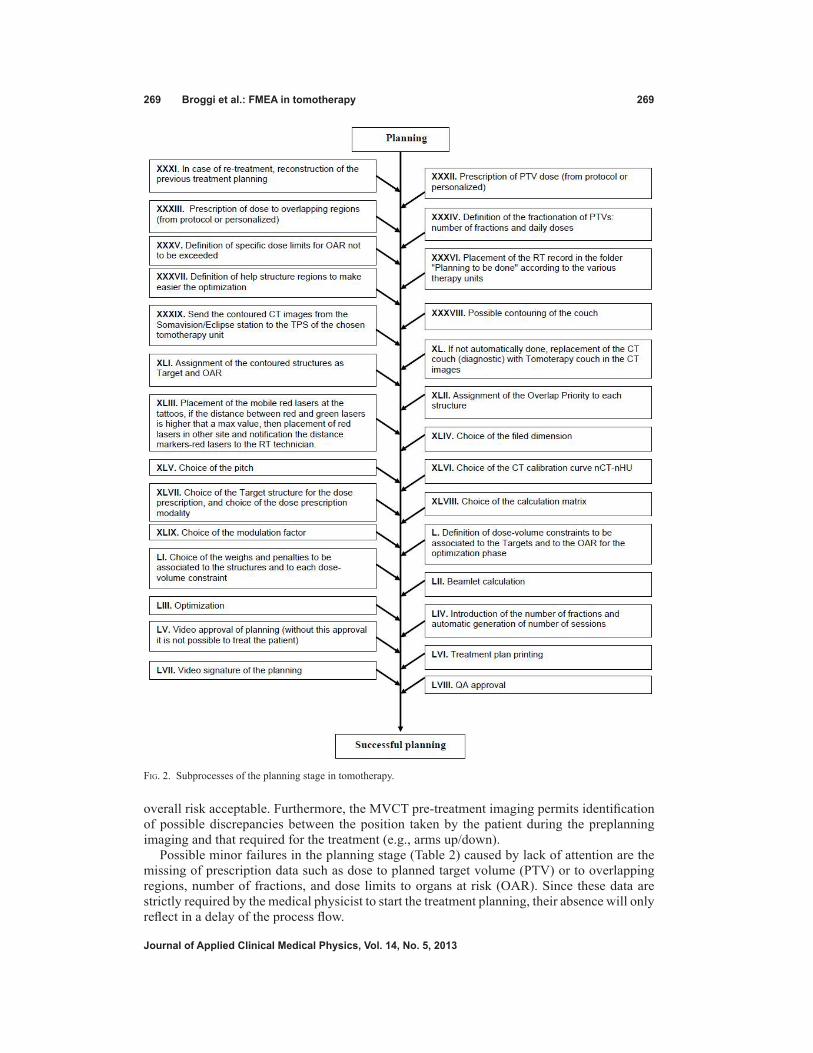
269 Broggi et al.: FMEA in tomotherapy 269
Journal of Applied clinical Medical Physics, Vol. 14, no. 5, 2013
overall risk acceptable. Furthermore, the MVCT pre-treatment imaging permits identification of possible discrepancies between the position taken by the patient during the preplanning imaging and that required for the treatment (e.g., arms up/down).
Possible minor failures in the planning stage (Table 2) caused by lack of attention are the missing of prescription data such as dose to planned target volume (PTV) or to overlapping regions, number of fractions, and dose limits to organs at risk (OAR). Since these data are strictly required by the medical physicist to start the treatment planning, their absence will only reflect in a delay of the process flow.
Fig. 2. Subprocesses of the planning stage in tomotherapy.
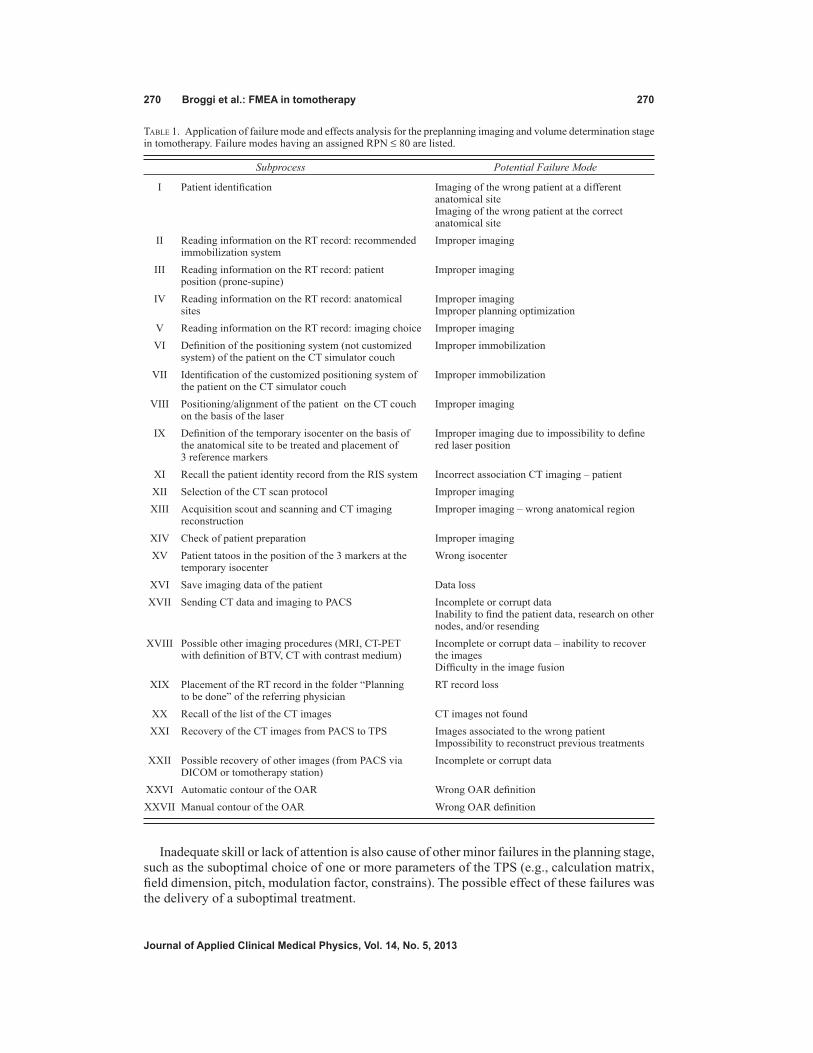
270 Broggi et al.: FMEA in tomotherapy 270
Journal of Applied clinical Medical Physics, Vol. 14, no. 5, 2013
Inadequate skill or lack of attention is also cause of other minor failures in the planning stage, such as the suboptimal choice of one or more parameters of the TPS (e.g., calculation matrix, field dimension, pitch, modulation factor, constrains). The possible effect of these failures was the delivery of a suboptimal treatment.
Table 1. Application of failure mode and effects analysis for the preplanning imaging and volume determination stage in tomotherapy. Failure modes having an assigned RPN ≤ 80 are listed.
Subprocess Potential Failure Mode
I Patient identification Imaging of the wrong patient at a different anatomical site
Imaging of the wrong patient at the correct anatomical site
II Reading information on the RT record: recommended Improper imaging immobilization system III Reading information on the RT record: patient Improper imaging position (prone-supine) IV Reading information on the RT record: anatomical Improper imaging sites Improper planning optimization V Reading information on the RT record: imaging choice Improper imaging VI Definition of the positioning system (not customized Improper immobilization system) of the patient on the CT simulator couch VII Identification of the customized positioning system of Improper immobilization the patient on the CT simulator couch VIII Positioning/alignment of the patient on the CT couch Improper imaging on the basis of the laser IX Definition of the temporary isocenter on the basis of Improper imaging due to impossibility to define the anatomical site to be treated and placement of red laser position 3 reference markers XI Recall the patient identity record from the RIS system Incorrect association CT imaging – patient XII Selection of the CT scan protocol Improper imaging XIII Acquisition scout and scanning and CT imaging Improper imaging – wrong anatomical region reconstruction XIV Check of patient preparation Improper imaging XV Patient tatoos in the position of the 3 markers at the Wrong isocenter temporary isocenter XVI Save imaging data of the patient Data loss XVII Sending CT data and imaging to PACS Incomplete or corrupt data Inability to find the patient data, research on other
nodes, and/or resending XVIII Possible other imaging procedures (MRI, CT-PET Incomplete or corrupt data – inability to recover with definition of BTV, CT with contrast medium) the images Difficulty in the image fusion XIX Placement of the RT record in the folder “Planning RT record loss to be done” of the referring physician XX Recall of the list of the CT images CT images not found XXI Recovery of the CT images from PACS to TPS Images associated to the wrong patient Impossibility to reconstruct previous treatments XXII Possible recovery of other images (from PACS via Incomplete or corrupt data DICOM or tomotherapy station) XXVI Automatic contour of the OAR Wrong OAR definition XXVII Manual contour of the OAR Wrong OAR definition

271 Broggi et al.: FMEA in tomotherapy 271
Journal of Applied clinical Medical Physics, Vol. 14, no. 5, 2013
Twenty-one failure modes (28% of cases) were characterized by a RPN score higher than 80. Ten of them, shown in Table 3, were identified in the stage of preplanning imaging and volume determination. The remaining 11 failures, which may occur during the stage of plan-ning, are shown in Table 4. The mean values of the risk indexes of Table 3 were O = 3.3 (range 3–4), S = 6.7 (range 5–8), and D = 4.8 (rage 3–6). Similarly, the mean values of the indexes of Table 4 were: O = 2.7 (range 2–4), S = 7.0 (range 5–8), and D = 6.2 (range 4–9). These data suggest that such events, on average, are infrequent (once or a few times a year) and not too difficult to detect (especially for the stage of preplanning imaging and volume determination), but potentially severe in terms of patient safety. The threshold of 125 for RPN was exceeded
Table 2. Application of failure mode and effects analysis for the planning stage in tomotherapy. Failure modes having an assigned RPN ≤ 80 are listed.
Subprocess Potential Failure Mode
XXXI In case of retreatment, reconstruction of the previous Wrong reconstruction treatment planning Reconstruction not possible Reconstruction suboptimal XXXII Prescription of PTV dose (from protocol or personalized) Missing prescription in the record XXXIII Prescription of dose to overlapping regions (from protocol Missing prescription in the record or personalized) XXXIV Definition of the fractionation of PTVs: number of fractions Missing prescription in the record and daily doses XXXV Definition of specific dose limits for OAR not to be Missing prescription in the record exceeded XXXVI Placement of the RT record in the folder “Planning to be Missing record done” according to the various therapy units. Planning for the wrong unit XXXVII Definition of help structure regions to make easier the Incorrect help structure region definition optimization XXXIX Send the contoured CT images from the Somavision/Eclipse Wrong data sent station to the TPS of the chosen tomotherapy unit XLI Assignment of the contoured structures as target and OAR Wrong assignment XLIII Placement of the mobile red lasers at the tattoos, if the Wrong positioning distance between red and green lasers is higher that a
max value, then placement of red lasers in other site and notification the distance markers/red lasers to the RT technician.
XLIV Choice of the filed dimension Suboptimal choice XLV Choice of the pitch Suboptimal choice XLVII Choice of the target structure for the dose prescription, Wrong choice and choice of the dose prescription modality XLIX Choice of the modulation factor Suboptimal choice L Definition of dose-volume constraints to be associated to Suboptimal choice the targets and to the OAR for the optimization phase LI Choice of the weights and penalties to be associated to Suboptimal choice the structures and to each dose-volume constraint LII Beamlet calculation Beamlet recalculation LIII Optimization Incomplete optimization LV Video approval of planning (without this approval it is Approval missing not possible to treat the patient) LVI Treatment plan printing Printed copy of the treatment plan missing LVII Video signature of the planning Signature missing LVIII QA approval QA approval missing

272 Broggi et al.: FMEA in tomotherapy 272
Journal of Applied clinical Medical Physics, Vol. 14, no. 5, 2013
in four cases: one case only in the phase of preplanning imaging and volume determination, and three cases in the stage of planning. Actually, treatment planning is known to be one of the most critical phases within the whole RT process.(9)
Table 3. Application of failure mode and effects analysis for the preplanning imaging and volume determination stage in tomotherapy. Failure modes having an assigned RPN > 80 are reported.
Potential Potential Causes Potential Effects Subprocess No Failure Mode of Failure of Failure O S D RPN
VIII Positioning/alignment Wrong Inadequate Systematic
of the patient on the 1 definition CT shift of the 4 8 3 96
CT couch on the basis of the laser patient
of the laser isocenter alignment position
X Reference markers Missing
Lack of attention Previous treatment
positioning to 2 marker or incomplete not taken into 4 6 3 96
indicate previous positions compilation of consideration/
treatment fields the RT record suboptimal planning
XXIII Registration of possible other 3 Wrong Consistency Wrong PTV and 3 7 5 105 images from different registration not verified OAR definition techniques and check of consistency
XXIV Definition of the GTVs and/or CTVs contour on the basis 4 Wrong CTV Lack of attention/ Wrong dose 3 7 5 105 of the anatomical definition inadequate skill distribution
and/or functional information (BTV)
XXV Definition of ITV Incorrect ITV Lack of attention/ in the case of 4D 5 construction inadequate skill Wrong PTV 3 6 5 90
CT acquisition
XXVI Automatic Missing OAR Lack of attention/ Unintended normal contour of the 6 definition inadequate skill tissue irradiation 3 8 5 120
OAR
XXVII Manual contour 7 Missing OAR Lack of attention/ Unintended normal 3 8 5 120 of the OAR definition inadequate skill tissue irradiation
XXVIII Definition of the planning structure Wrong Lack of attention/ Unintended normal at risk through 8 expansion inadequate skill tissue irradiation 3 5 6 96
automatic expansion of OAR
XXIX Automatic expansion with definition of the 9 Wrong Lack of attention/ Unintended normal 3 5 6 96 CTVs and PTVs expansion inadequate skill tissue irradiation margins
XXX Lack of attention/ Definition and Wrong/missed inadequate skill Unintended normal
contouring of 10 definition or not detailed tissue irradiation 4 7 5 140 overlapping information on or wrong dose regions previous treatment distribution

273 Broggi et al.: FMEA in tomotherapy 273
Journal of Applied clinical Medical Physics, Vol. 14, no. 5, 2013
Table 4. Application of failure mode and effects analysis for the planning stage in tomotherapy. Failure modes having an assigned RPN > 80 are reported.
Potential Potential Causes Potential Effects Subprocess No Failure Mode of Failure of Failure O S D RPN
XXXII Prescription of Wrong Lack of attention/ Wrong dose PTV dose (from 11 prescription inadequate skill delivery 3 8 4 96 protocol or in the record personalized)
XXXIII Prescription of Possible wrong dose to overlapping 12
Wrong Lack of attention/ dose distribution/ regions (from prescription inadequate skill wrong dose 3 8 4 96
protocol or in the record delivery personalized)
XXXIV Definition of the Wrong fractionation of 13 prescription Lack of attention/ Wrong dose 3 8 4 96 PTVs: number in the record inadequate skill delivery of fractions and daily doses
XXXV Definition of Wrong Lack of attention/ Unintended normal specific dose limits 14 prescription inadequate skill tissue irradiated 3 8 4 96 for OAR, not in the record to be exceeded
XXXVIII Incorrect Possible contouring 15 Incorrect dose positioning in Wrong dose 2 6 7 84 of the couch calculation the imaging delivery
XL If not automatically done, replacement Incorrect dose Incorrect introduction Wrong dose in the imaging of 16 calculation of the couch position delivery 2 6 8 96 the CT couch in the CT images (diagnostic) with tomoterapy couch
XLII Assignment of the 17 Wrong Lack of attention/ Wrong dose 4 7 7 196 Overlap Priority assignment inadequate skill distribution to each structure
Wrong dose XLVI 18 Wrong choice Lack of attention/ calculation/wrong 2 8 9 144 Choice of the (kV-MV) inadequate skill dose delivery calibration curve 19 Wrong choice Lack of attention/ Wrong dose 2 5 9 90 nCT-nHU (kV-kV) inadequate skill calculation/wrong dose delivery
XLVIII Choice of the 20 Suboptimal Lack of attention/ Suboptimal 3 5 6 90 calculation matrix choice inadequate skill treatment
LIV Introduction Wrong or not of the number performed choice Lack of attention/ Wrong dose of fractions and 21 (erroneous use of inadequate skill delivery 3 8 6 144 automatic generation the default value) of number of sessions

274 Broggi et al.: FMEA in tomotherapy 274
Journal of Applied clinical Medical Physics, Vol. 14, no. 5, 2013
The failure mode with the highest risk (i.e., RPN = 140) within the stage of preplanning imaging and volume determination was the wrong or missing definition and contouring of the overlapping regions. Overlapping regions are, in general, defined to limit the prescription dose to some structures, both in case of overlapping between target volume and dose limit to organs at risk, and in case of retreatment. Typical examples of overlapping regions are the boundaries between PTV and chiasma and/or optical structures, PTV and anterior rectal wall, and PTV and duodenum and/or stomach. In tomotherapy, the overlapping regions of adjacent anatomical structures need to be defined and contoured, and a priority level has to be assigned during planning in order to achieve the correct dose distribution to the PTV and, at the same time, to spare the OAR.
If one or more overlapping regions are not properly defined or contoured by the radiation oncologist, the potential effect for the patient could be an unintended normal tissue irradiation or, more likely, a wrong dose distribution. The main cause of this failure was identified as a lack of attention or inadequate skill of the radiation oncologist in charge of defining and con-touring the volumes of interest. Moreover, this failure might occur as a consequence of a lack of exhaustive clinical documentation about possible previous RT treatments. Indeed, the doses received by the various anatomical structures during previous irradiations have to be taken into account for defining the overlapping regions.
An additional safety measure was suggested by the working group for reducing the prob-ability of occurrence of this failure, and therefore for mitigating the overall risk. It consisted of improving the RT record of the patient through the systematic introduction of a sheet to be flagged containing detailed information about the prescribed dose to target volumes, OARs, and overlapping regions contoured with relative dose constraints.
The most critical failure in the stage of planning (RPN = 196) was the wrong assignment of the overlap priority to each anatomical structure by the medical physicist. The TPS prompts the user to divide structures or regions of interest (ROI) into two groups: tumors and organs at risk. A ROI from the tumor group can overlap with a ROI in the OAR group, but the ROIs within the same group are not allowed to own common voxels. When two contours from the same group overlap with each other, the overlap priority setting governs to which structure the voxel belongs. The structure with the higher overlap priority will own the voxels in the overlap region, and the structure with lower overlap priority will lose these voxels for dose volume computations, optimization, and dose-volume histograms (DVHs) in the overlapping mode visualization.(19) Therefore, overlap priorities must be carefully selected since, in case of failure, wrong dose optimization can be generated with possible serious consequences for the patient. As for many other failures, this error was recognized as the result of a lack of attention or inadequate skill of the medical physicist in charge of planning. The probability of this failure going undetected was estimated to be relatively high if the final plan evaluation is based on only the DVH in the overlapping mode (i.e., the usual way to visualize the DVH during plan optimization). For this reason, the additional safety measure recommended by the WG consisted of a systematic final plan evaluation considering both the DVH in the overlapping mode and in the standard mode (i.e., the mode that provides the statistics of the entire volumes), regardless the defined overlapping priorities. It is interesting to note that the possibility to visualize and to print out the DVHs in the two different modes is an option of one of the latest TPS release.
A further critical failure identified in the planning stage (RPN = 144) was the wrong choice of the CT calibration curve. This failure might accordingly occur when more than one CT scanning system is available, each of them with the proper calibration curve. Since the dose calculation process by the TPS is based on the data of the CT calibration, the wrong choice of calibration curve could reflect in a wrong dose calculation and, possibly, in a wrong dose delivery. This failure could be particularly critical in tomotherapy since, in the case of using MVCT instead of kVCT images, or vice-versa, a significant variation in the calculated dose (i.e., of the order of 10%) is expected. Indeed, the relationship of MVCT number to electron density is different

275 Broggi et al.: FMEA in tomotherapy 275
Journal of Applied clinical Medical Physics, Vol. 14, no. 5, 2013
from that observed in common kVCT scanners as a consequence of the difference in physical interaction probabilities of photons within the two energy ranges.
This failure was considered extremely hard to detect (i.e., D = 9). Indeed, the information about the CT calibration curve chosen for dose calculation cannot be included in the printed copy of the treatment plan. Therefore, the correctness of this parameter cannot be checked dur-ing the plan evaluation before the final approval. On the basis of this analysis, the WG decided, as additional strategy, to suggest the vendor implement a new function in the TPS software, consisting of the possibility for the user to include the information on the CT calibration curve in the printed copy of the treatment plan.
The last major failure (with a RPN = 144) which might occur during the planning stage, was the wrong (or not performed) choice of the number of fractions composing the treatments. A default number of fractions equal to 30 is set in the TPS. This value must be changed by the planner according to the particular prescription. If the planner fails to perform this task, the consequences for the patient could be particularly severe, since a wrong daily dose could be delivered during the treatment. The additional safety measure recommended by the WG is to increase the probability of failure detection by the RT technician before the treatment start through the systematic check of the agreement between the number of fractions actually prescribed in the radiotherapy sheet and the number of procedures visualized on the screen of the tomotherapy control unit.
In addition to the failure modes with the highest overall risks, specific attention should be paid to the failures which could lead to severe injuries to the patients, independently of the RPN value. In this analysis, seven failure modes characterized by a severity index S = 8 and RPN < 125 were identified (i.e., failures No. 1, 6 and 7 in Table 3 and Nos. 11-14 in Table 4). The wrong definition of the isocenter during the positioning of the patient on the CT couch, even though potentially dangerous, appeared easily detectable, since the laser alignment is daily checked through the use of the MVCT scanner. No further safety measures are, therefore, required.
The risk of missing OAR definitions can be simply mitigated through the implementation of the safety measures formerly proposed. In particular, the suggested improvement of the RT record could significantly reduce the number of occurrences of these failures.
Finally, additional safety measures are required to deal with the remaining failures — the wrong prescription of dose and/or dose limits. Systematic double-check of these data by the radiation therapy staff, and/or the definition of reference protocols, could be an adequate solu-tion increasing the detection rating of these failures.
The failure modes shown in Tables 1–4 were identified by analyzing the typical sequence of events and procedures that characterize the standard RT process. However, in clinical prac-tice, some deviations from the standard process flow might occur as a consequence of specific medical or organizational needs. Unfortunately, such process changes cannot be considered free from additional potential failures. In particular, three events which could affect the patient safety were identified by the working group and are briefly described below.
1. When the prescribed dose to the PTV is high, it may occur that the HTU is not able to deliver the entire dose in a single fraction; the physicist has to duplicate the number of fractions and write in the radiotherapy sheet to deliver two fractions every daily treatment session. If the indication is not clearly reported, this can result in an uncorrected daily dose delivery to the patient.
2. Sometimes, it could happen that the radiation oncologist decides to deliver more fractions than planned (e.g., if the treatment needs to be interrupted in a case where the patient expe-rienced severe side effects). The TPS does not allow the physicist to add treatment fractions without replanning and recalculating the plan, but only those QA fractions on the operator station. So the patient can be treated, but the final treatment report does not record the added fractions and only the radiotherapy sheet can attest the real delivered dose.
276 Broggi et al.: FMEA in tomotherapy 276
Journal of Applied clinical Medical Physics, Vol. 14, no. 5, 2013
3. As previously reported, at San Raffaele Scientific Institute two HTUs are currently operat-ing. The two machines are twinned in order to have the possibility to transfer the patient from one unit to the other one (in a case where one machine needs maintenance). In such a case, the patient should be immediately cancelled from the original unit, transferred to the second one, treated, deleted from the TPS of the second unit, and finally transferred again to the original unit. In fact, this procedure would permit the tracking of the treatments actu-ally done by the patient on the two units. However, it must be considered that every transfer entails a new final dose calculation (taking into account the specific output factors and MLC mechanical characteristics of each unit); moreover, each of these operations takes a lot of time to be completed. So, usually the patient record remains simultaneously on the two TPS for few days and, in this way, the only possibility to check the number of fractions actually delivered is through the radiotherapy sheet of the patient.
In all these circumstances, more flexibility of the system should let the operator to modify the schedule of the treatment so as to avoid communication errors that can induce an incorrect dose to patients. One solution could be the implementation of a record and verify system; a session, daily, and total dose accumulation point could also be a safety issue.
In addition to the safety measures specifically related to tomotherapy proposed by the WG, the results of this analysis confirmed the soundness of the general lessons and recommenda-tions provided by ICRP for preventing accidental exposures from new external beam radiation therapy technologies.(10) Indeed, during the identification of the causes of failures and the estimation of their occurrence probability, it came out that the competence and skill of the various professional figures involved in the RT process, as well as the work environment, play an important role both for the quality of the treatment and for patient safety. Regular updating of the knowledge and maintenance of the skills of the personnel can, therefore, represent an efficient instrument for patient safety improvement. In particular, the development of specific professional training schemes on the functionalities and limits of the various systems and software used in the RT process, as well as on the procedures and protocols, can be considered a general action for reducing the frequency of failures and, consequently, the overall risk of accidents in tomotherapy. Furthermore, excessive workload should be avoided, and a suitable work environment that encourages working with awareness, facilitates concentration, and avoids distraction should be provided.
Finally, as in other modern RT techniques, in tomotherapy in vivo dosimetry could provide a reliable way of detecting serious anomalies potentially leading to substantial overdoses or underdoses to the patient.
IV. concLuSIonS
The application of FMEA to the preplanning imaging, volume determination, and treatment planning stages in tomotherapy led to the identification and deep investigation of various failure modes. The assignment of a score assessing the potential risk for each event permitted a ranking of these failure modes in order of importance and the ability to define priorities for risk mitigation, with the aim of optimizing quality management workflow. In addition to the safety strategies already adopted in the clinical practice, novel solutions have been proposed to increase patient safety.
Although this study was carried out considering the specific processes implemented at San Raffaele Scientific Institute, the proposed methodology, as well as likely most of the findings, can be generalized and made useful to other RT centers equipped with HTU.
On the basis of the results obtained in this study and of the experience accrued by the WG,(20) further stages of the RT process, such as treatment delivery and treatment monitoring and veri-fication, will be analyzed by means of the FMEA approach in the near future.

277 Broggi et al.: FMEA in tomotherapy 277
Journal of Applied clinical Medical Physics, Vol. 14, no. 5, 2013
rEFErEncES
1. Hoeschen C, Mattsson S, Cantone MC, et al. Minimising activity and dose with enhanced image quality by radiopharmaceutical administrations. Rad Prot Dosimetry. 2010;139(1-3):250–53.
2. Mancosu P, Cozzi L, Fogliata A, et al. Collimator angle influence on dose distribution optimization for vertebral metastases using volumetric modulated arc therapy. Med Phys. 2010;37(8):4133–37.
3. Korreman S, Rasch C, McNair H, et al. The European Society of Therapeutic Radiology and Oncology-European Institute of Radiotherapy (ESTRO-EIR) report on 3D CT-based in-room image guidance systems: a practical and technical review and guide. Radiother Oncol. 2010;94(2):129–44.
4. Reggiori G, Mancosu P, Tozzi A, et al. Cone beam CT pre- and post-daily treatment for assessing geometrical and dosimetry intrafraction variability during radiotherapy of prostate cancer. J Appl Clin Med Phys. 2011;12(1):141–52.
5. Broggi S, Cattaneo GM, Molinelli S, et al. Results of a two-year quality control program for a helical tomotherapy unit. Radiother Oncol. 2008;86(2):231–41.
6. Veronese I, Cantone MC, Catalano M, et al. Study of the radioluminesence spectra of doped silica optical fibre dosimeters for stem effect removal. J Phys D Appl Phys. 2013;46(1):015101.
7. Veronese I, Cantone MC, Chiodini N, et al. Feasibility study for the use of cerium-doped silica fibres in proton therapy. Radiat Meas. 2010;45(3-6):635–39.
8. Veronese I, Cantone MC, Chiodini N, et al. The influence of the stem effect in Eu-doped silica optical fibres [online]. Radiat Meas. 2013. http://dx.doi.org/10.1016/j.radmeas.2013.01.043
9. World Health Organization. Radiotherapy risk profile. Geneva: WHO; 2008. 10. International Commission on Radiological Protection. Preventing accidental exposures from new external beam
radiation therapy technologies. Annals of the ICRP. 2009;39(4). 11. Ciocca M, Cantone MC, Veronese I, et al. Application of failure mode and effects analysis to intraoperative radi-
ation therapy using mobile electron linear accelerators. Int J Radiat Oncol Biol Phys. 2012;82(2):e305–e311. 12. Perks JR, Stanic S, Stern RL, et al. Failure mode and effect analysis for delivery of lung stereotactic body radi-
ation therapy. Int J Radiat Oncol Biol Phys. 2012;83(4):1324–29. 13. Sawant A, Dieterich S, Svatos M, Keall P. Failure mode and effect analysis-based quality assurance for dynamic
MLC tracking systems. Med Phys. 2010;37(12):6466–79. 14. Ekaette EU, Lee RC, Cooke DL, Iftody S, Craighead P. Probabilistic fault tree analysis of a radiation treatment
system. Risk Anal. 2007;27(6):1395–410. 15. Ford EC, Gaudette R, Myers L, et al. Evaluation of safety in radiation oncology setting using failure mode and
effects analysis. Int J Radiat Oncol Biol Phys. 2009;74(3):852–58. 16. Cantone MC, Ciocca M, Dionisi F, et al. Application of failure mode and effects analysis to treatment planning
in scanned proton beam radiotherapy. Radiat Oncol. 2013;8(1):127 [Epub ahead of print]. 17. Huq MS, Fraass BA, Dunscombe PB, et al. A method for evaluating quality assurance needs in radiation therapy.
Int J Radiat Oncol Biol Phys. 2008;71(1 Suppl):S170–S173. 18. United States Nuclear Regulatory Commission. Gamma knife treatment to wrong side of brain. Event Notification
Report 43746. Vienna: IAEA; 2007. 19. Langen KM, Papanikolaou N, Balog J, et al. QA for helical tomotherapy: report of the AAPM Task Group 148.
Med Phys. 2010;37(9):4817–53. 20. Begnozzi L, Cantone MC, Longobardi B, Veronese I. Prospective approaches for risk analysis in modern radio-
therapy: the Italian experience and the contribution of the medical physicists. Radioprotection 2013, doi: 10.1051/radiopro/2013079
a Corresponding author: Stewart J. Becker, Department of Radiation Oncology, Rm-103, NYU Langone Medical Center, 160 E. 34th St, New York, NY 10016, USA; phone: (212) 731-5827; fax: (212) 731-5551; email: [email protected]
Collision indicator charts for gantry-couch position combinations for Siemens ONCOR and Elekta Infinity linacs
Stewart J. Becker,1a Wes Culberson,2 and Ryan T. Flynn3
Radiation Oncology,1 NYU Langone Medical Center, New York, NY, USA; Santa Cruz Radiation Oncology,2 Santa Cruz, CA, USA; Radiation Oncology,3 University of Iowa Hospitals and Clinics, Iowa City, IA, [email protected]
Received 7 January, 2013; accepted 25 April, 2013
Noncoplanar radiation fields from a linear accelerator can be used to deliver radia-tion dose distributions that are superior to those delivered using coplanar radiation fields. Noncoplanar radiation field arrangements are especially valuable when delivering stereotactic body radiation therapy (SBRT). Noncoplanar radiation fields, however, are geometrically more challenging to deliver than coplanar radiation fields, and are associated with a greater risk of collisions between the gantry, treat-ment couch, and patient. Knowledge of which treatment couch offset, treatment couch angle, and gantry angle combinations provide a collision-free radiotherapy delivery is useful in the treatment planning process, as the risk of requiring replan-ning due to improperly selected treatment parameters can be minimized. Such tables are by default specific to the linear accelerator make and model used for treatment. In this work a set of plots is presented indicating which combination of treatment couch lateral offsets (-10 cm to 10 cm), couch angles (270° to 90°), and gantry angles (0° to 360°), will result in collision-free radiation delivery using Siemens ONCOR linear accelerators equipped with a 160-leaf multileaf collimator and a 550 TxT treatment table, and a Elekta Infinity linear accelerator with an MLCi2 and Elekta iBEAM evo Couchtop EP. The patient was assumed to have a width of 50 cm and a height of 25 cm.
PACS numbers: 87.55.-x, 87.56.-v
Key words: collision, treatment planning, gantry, couch, noncoplanar, Siemens ONCOR, Elekta Infinity
I. INtROduCtION
Noncoplanar radiation fields are useful for minimizing the volume of normal tissue receiv-ing high doses in patients receiving stereotactic body radiotherapy (SBRT).(1) In the external beam radiotherapy treatment planning process, it can be challenging to predict when colli-sions will occur between the linear accelerator gantry, treatment couch, and patient, especially when noncoplanar radiation fields are used. As reported in a previous paper on Varian linear accelerators (Palo Alto, CA),(2) small variations in treatment couch heights and lateral offsets can dramatically affect which gantry and treatment couch angles can be utilized for a given radiation field. In the current work, plots of gantry angle, treatment couch lateral offset, height, and angle combinations that are collision-free are presented for Siemens ONCOR (Erlangen, Germany) and Elekta Infinity (Stockholm, Sweden) linear accelerators.
JOuRNAL OF APPLIEd CLINICAL MEdICAL PHYSICS, VOLuME 14, NuMBER 5, 2013
278 278

279 Becker et al.: Gantry-couch collision chart 279
Journal of Applied Clinical Medical Physics, Vol. 14, No. 5, 2013
II. MAtERIALS ANd MEtHOdS
The measurements presented were acquired on two different accelerator platforms. The first was a Siemens ONCOR linear accelerator with a 160-leaf multileaf collimator and a 550 TxT treatment couch using methods described previously.(2) The second was an Elekta Infinity with an MLCi2 and iBEAM evo Couchtop EP. All gantry and treatment couch angles are expressed relative to an observer looking at the gantry from the foot of the treatment couch when it is in the 0° position. The treatment couch is at 0° when it is aligned parallel to the axis of gantry rotation, 90° when rotated to the observer’s right, and 270° to the observer’s left. The treatment couch can be offset to the observer’s right (positive) and left (negative). The gantry angle is 0° when the radiation field is pointing vertically down, and the gantry angle increases as the gantry rotates clockwise relative to its axis. This system corresponds to the IEC 1217, with the exception of the couch vertical which is expressed as positive going down compared to nega-tive (in IEC 1217). Treatment couch positions were measured between 90° and 270° crossing through 0°. Treatment couch vertical positions of 10, 15, and 20 cm below the axis of gantry rotation and lateral treatment couch offsets of 0 and ± 10 cm were selected since they encompass the majority of clinical situations. Symmetry was verified for both machines (e.g., gantry 75°, couch 30° is equal to gantry 285°, couch 330°).
The maximum couch angle achievable for each gantry position was determined by first rotat-ing the gantry to a position and then rotating the couch such that it was within 1° of colliding with the gantry. Measurements were taken at higher sampling rate near collision zones, and the gantry angle sampling frequency was at least 5°. For the Siemens platform, the patient’s pres-ence was simulated by placing typical vacuum-based immobilization systems on the treatment couch, which had a height of 25 cm and a width of 50 cm. For the Elekta platform, an Eelkta BodyFix immobilization system was used with the compression paddle attachment in place. Any near-collisions with the immobilization systems were assumed to be patient collisions also.
III. RESuLtS
Figures 1–3 pertain to treatment couch lateral offsets of 0 cm, +10 cm, and -10 cm, respectively, for a Siemens linac and couch, and show the corresponding allowable gantry angles, treatment couch angles, and treatment couch heights. Figures 4–6 show similar data for an Elekta linac/couch combination. The area inside the curves, including the origin, is the “collision free” zone.

280 Becker et al.: Gantry-couch collision chart 280
Journal of Applied Clinical Medical Physics, Vol. 14, No. 5, 2013
Fig. 1. Siemens couch vs. gantry chart for vertical couch positions of 10 cm (blue), 15 cm (black), and 20 cm (magenta), lateral offset of 0 cm, and couch rotations from 0° to 90° (black) and 360°–270° (blue). Every angle inside the lines (including the origin) is collision free.
Fig. 2. Siemens couch vs. gantry chart for vertical couch positions of 10 cm (blue), 15 cm (black), and 20 cm (magenta), lateral offsets of 10 cm in the direction of the couch angle swing. Every angle inside the lines (including the origin) is collision free.

281 Becker et al.: Gantry-couch collision chart 281
Journal of Applied Clinical Medical Physics, Vol. 14, No. 5, 2013
Fig. 3. Siemens couch vs. gantry chart for vertical couch positions of 10 cm (blue), 15 cm (black), and 20 cm (magenta), lateral offsets of 10 cm in the opposite direction of the couch angle swing. Every angle inside the lines (including the origin) is collision free.
Fig. 4. Elekta couch vs. gantry chart for vertical couch positions of 10 cm (blue), 15 cm (black), and 20 cm (magenta), lateral offset of 0 cm, and couch rotations from 0° to 90° (black) and 360°–270° (blue). Every angle inside the lines (including the origin) is collision free.

282 Becker et al.: Gantry-couch collision chart 282
Journal of Applied Clinical Medical Physics, Vol. 14, No. 5, 2013
Fig. 5. Elekta couch vs. gantry chart for vertical couch positions of 10 cm (blue), 15 cm (black), and 20 cm (magenta), lateral offsets of 10 cm in the direction of the couch angle swing. Every angle inside the lines (including the origin) is collision free.
Fig. 6. Elekta couch vs. gantry chart for vertical couch positions of 10 cm (blue), 15 cm (black), and 20 cm (magenta), lateral offsets of 10 cm in the opposite direction of the couch angle swing. Every angle inside the lines (including the origin) is collision free.

283 Becker et al.: Gantry-couch collision chart 283
Journal of Applied Clinical Medical Physics, Vol. 14, No. 5, 2013
IV. dISCuSSION & CONCLuSIONS
The most conservative estimate for a collision-free couch angle at a given gantry angle, treatment couch height and treatment couch offset may be read from the appropriate plot by finding the gantry angle on the outside of the polar plot and tracing toward the origin to find the treatment couch angle. The most conservative estimate for safe gantry-couch angle combination is not always associated with the same couch height, which reflects consideration for anterior versus posterior oblique gantry angles.
When the couch is rotated towards the gantry, the gantry always collides with the base of the couch regardless of which vertical treatment couch position is used. For treatment couch heights of 20 cm below isocenter, the collision occurs sooner than for 15 cm or less due to the presence of pendant holders on the left and right of the Siemens 550 TXT couch. For instance in Fig. 1, the couch and gantry do not collide at couch height of 10 cm or 15 cm when the gantry is 175° and a couch angle is 90°; however, if the couch height is dropped to 20 cm, there will be a collision at that same gantry and couch angles.
The Elekta couch has the option to fold the pendant out of the way and, therefore, it behaves in a much more predictable manner.
ACkNOwLEdGMENtS
The authors wish to thank Celeste Leary from Santa Cruz Radiation Oncology for helping perform the measurements.
REFERENCES
1. Benedict SH, Yenice KM, Followill D, et al. Stereotactic body radiation therapy: the report of AAPM Task Group 101. Med Phys. 2010;37(8):4078–101.
2. Becker SJ. Collision indicator charts for gantry-couch position combinations for Varian linacs. J Appl Clin Med Phys. 2011;12(3):3405.