Does transfer to intensive care units reduce mortality for deteriorating ward patients? Estimating Person-centered Treatment (PeT) effects using instrumental variables

Does transfer to intensive care units reduce mortality for deteriorating ward patients?

Estimating Person-centered Treatment (PeT) Effects Using Instrumental Variables

Anirban BasuUniversity of Washington, Seattle

(Joint work with Stephen O’Neill, National University of Ireland Galway and Richard Grieve, London School of Hygiene and Tropical Medicine)

Treatment Evaluations• Literature on treatments effects focused on informing

population level or policy-level decisions.o Mean effectso Distributional effectso Impacts are viewed as informing a social decision maker to

help choose across alternative optionso Discussions will focus on evaluating policies/treatment in use

• Heterogeneity: Optimal Individual choices may vary from socially optimal choices, based on ex-postrealizations.

1

Literature on Distribution of Treatment Effects

• Imbens and Rubin (1997) and Abadie (2002, 2003) • Carniero and Lee (2009) • Heckman and Honoré 1990, Heckman and Smith

1993, Heckman et al. 1997.• Factor structure models have been used to

establish the joint distribution of potential outcomes (Aakvik et al. 1999, Carniero et al. 2003).

• Importance of distribution of effects well established in the literature (Abbring and Heckman, 2007)

2

Healthcare Setting• Dilemma between social versus individual choices,

perhaps, the most stark• In traditional clinical outcomes research, the focus

has always been on finding average effects either through large clinical trials or observational datasets.

• Estimating treatment effect heterogeneity has mostly been relegated to post-hoc analysis, rather than becoming the central goal of the analysis.

• Growing recognition of the importance of nuanced and possibly individualized estimates of treatment effects (Basu 2009, 2011, Basu et al. 2011).

3

Observational Data Setting• Observational data is a valuable resource.

• Selection bias in observational studies is a potential problem – primary reason for relegation to second-tier status in evidentiary standards.

• However, growing interests due to large scale investments in Electronic Health Records.

• Methods for casual inference in such data of high demand.

4

Outline• Conceptual Identification of treatment effects using

instrumental variable methods

• PeT effects

• PeT effects estimation

• Empirical Example

5

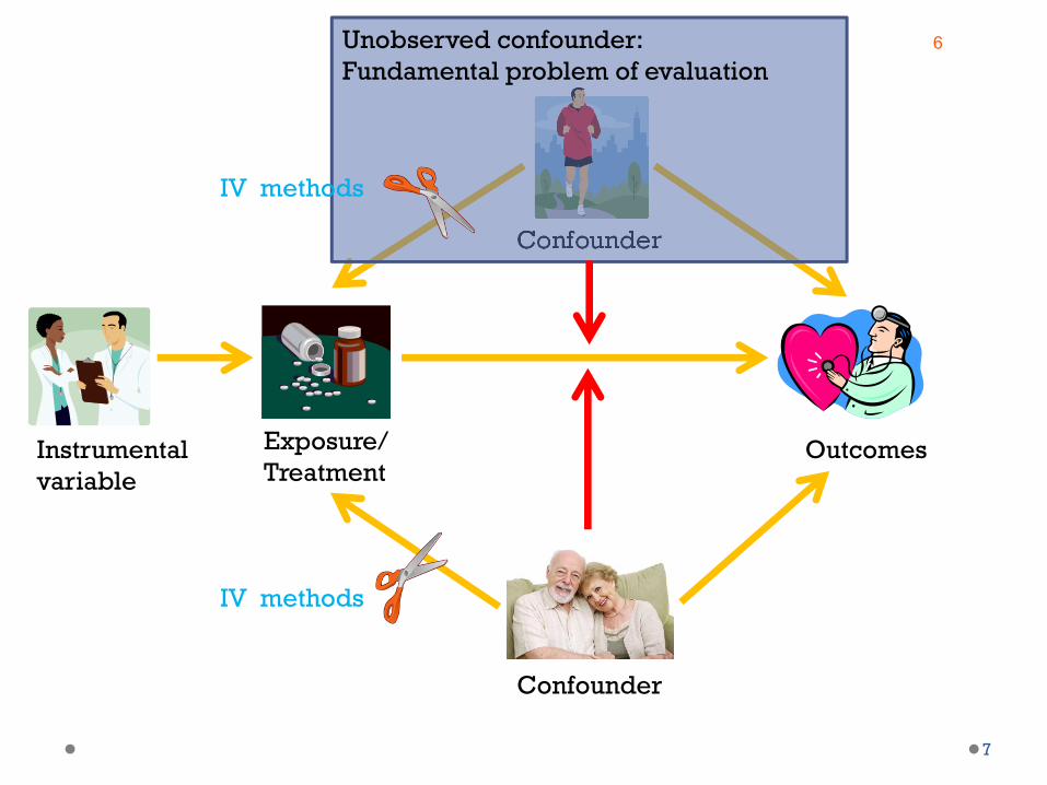
Exposure/ Treatment

Outcomes

Confounder

Confounder

Unobserved confounder: Fundamental problem of evaluation

Instrumental variable

IV methods

IV methods

7

6

Stylized example• Treatments (D): Surgery versus watchful waiting• Outcomes (Y): Mortality or recurrence or costs• Unobserved Confounder: Disease severity

(all observed confounder are adjusted for)

• Instrumental variable: Distance to hospital

7

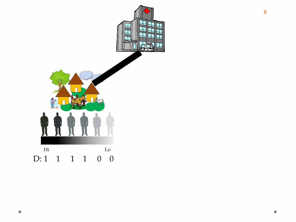
Hi Lo

D: 1 1 1 1 0 0

8

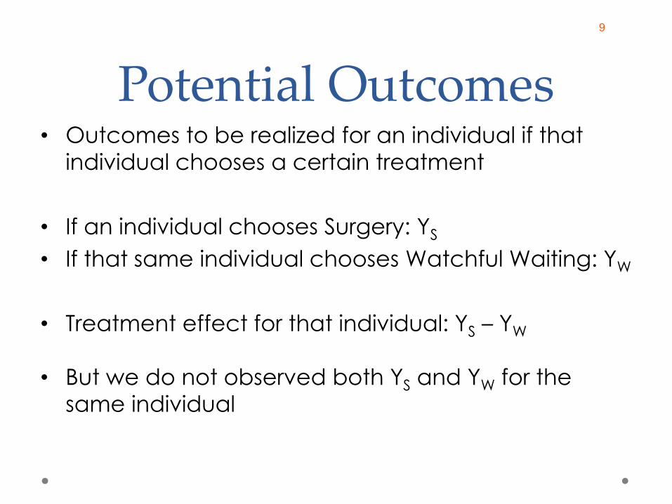
Potential Outcomes• Outcomes to be realized for an individual if that

individual chooses a certain treatment

• If an individual chooses Surgery: YS

• If that same individual chooses Watchful Waiting: YW

• Treatment effect for that individual: YS – YW

• But we do not observed both YS and YW for the same individual

9

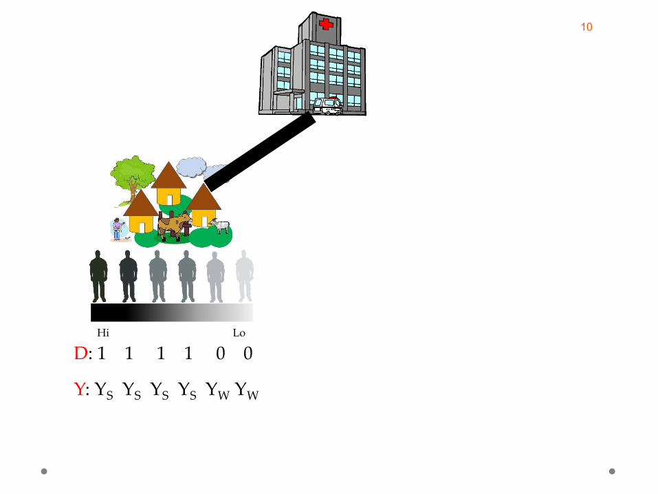
Hi Lo

D: 1 1 1 1 0 0

Y: YS YS YS YS YW YW

10

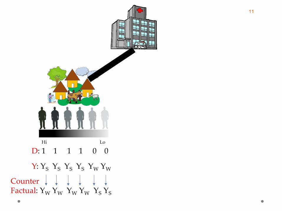
Hi Lo

D: 1 1 1 1 0 0


CounterFactual: YW YW YW YW YS YS

11

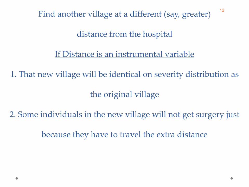
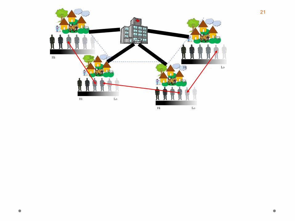
Find another village at a different (say, greater)

distance from the hospital

If Distance is an instrumental variable

1. That new village will be identical on severity distribution as

the original village

2. Some individuals in the new village will not get surgery just

because they have to travel the extra distance

12

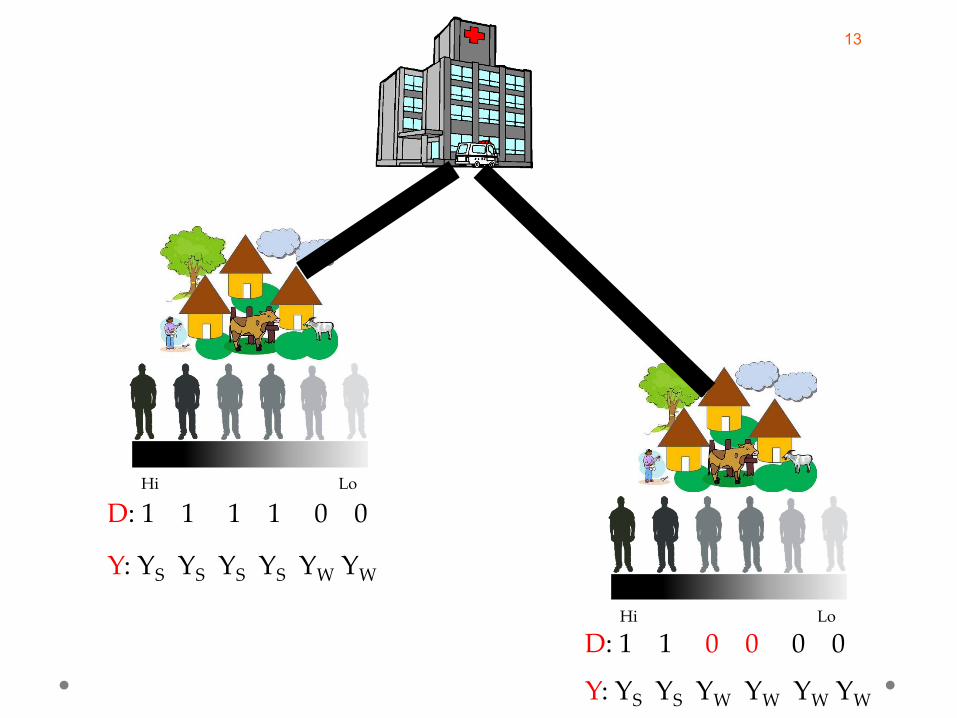
Hi Lo

D: 1 1 1 1 0 0


Hi Lo

D: 1 1 0 0 0 0

Y: YS YS YW YW YW YW

13

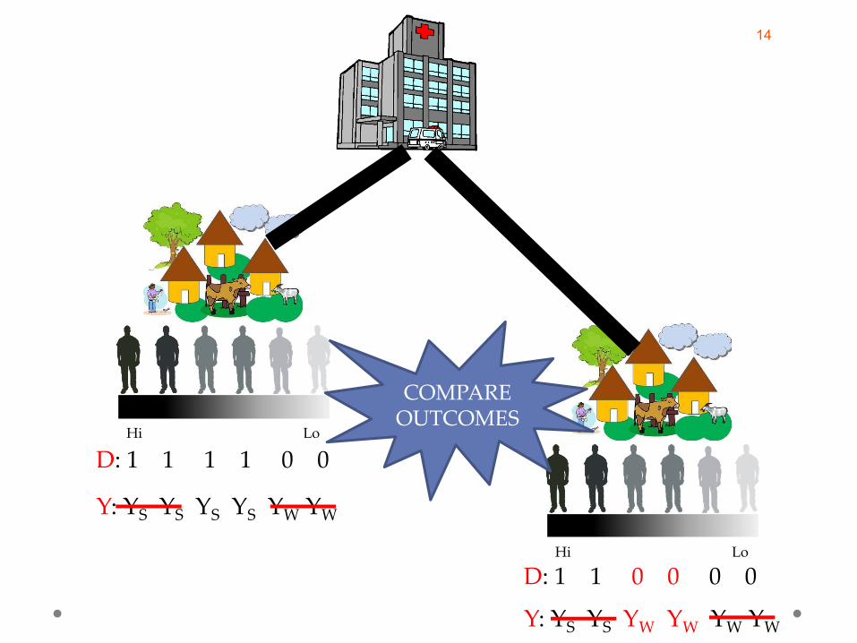
Hi Lo

D: 1 1 1 1 0 0


Hi Lo

D: 1 1 0 0 0 0

Y: YS YS YW YW YW YW

COMPAREOUTCOMES

14

IV effect• With two levels of an IV (e.g. short distance vs long

distance):o IV effect produces the causal effect for a group of

individuals, whose treatment choices are altered because of the change of the IV levels

o Local Average Treatment effect (Angrist and Rubin 1996)

o Challenges:• Who are these people (remember we don’t observed

severity in the data)?• How generalizable are there effects to other?

o If treatment effects vary over severity, LATE is NOT a very useful result.

15

Where is LATE useful?• Where the binary instrument represents a policy

change..• E.g. Oregon lottery as a instruments for Medicaid

receipt• LATE = the average effects on outcomes on those

who choose to get Medicaid if Medicaid eligibility were to be expanded

16

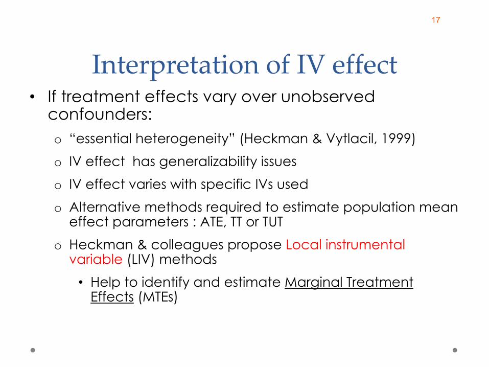
Interpretation of IV effect• If treatment effects vary over unobserved

confounders:o “essential heterogeneity” (Heckman & Vytlacil, 1999)o IV effect has generalizability issueso IV effect varies with specific IVs usedo Alternative methods required to estimate population mean

effect parameters : ATE, TT or TUTo Heckman & colleagues propose Local instrumental

variable (LIV) methods• Help to identify and estimate Marginal Treatment

Effects (MTEs)

17

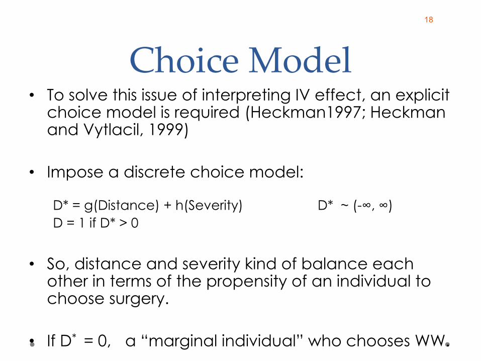
Choice Model• To solve this issue of interpreting IV effect, an explicit

choice model is required (Heckman1997; Heckman and Vytlacil, 1999)

• Impose a discrete choice model:

D* = g(Distance) + h(Severity) D* ~ (-∞, ∞)D = 1 if D* > 0

• So, distance and severity kind of balance each other in terms of the propensity of an individual to choose surgery.

• If D* = 0, a “marginal individual” who chooses WW.

18

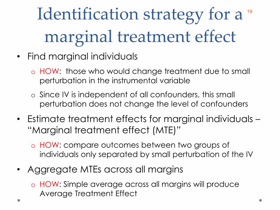
Identification strategy for a marginal treatment effect

• Find marginal individualso HOW: those who would change treatment due to small

perturbation in the instrumental variable

o Since IV is independent of all confounders, this small perturbation does not change the level of confounders

• Estimate treatment effects for marginal individuals –“Marginal treatment effect (MTE)”o HOW: compare outcomes between two groups of

individuals only separated by small perturbation of the IV

• Aggregate MTEs across all marginso HOW: Simple average across all margins will produce

Average Treatment Effect

19

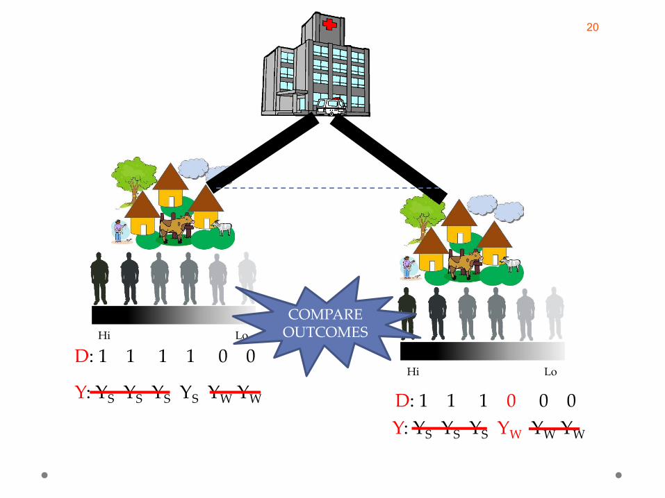
Hi Lo

D: 1 1 1 1 0 0


Hi Lo

D: 1 1 1 0 0 0Y: YS YS YS YW YW YW

COMPAREOUTCOMES

20

21

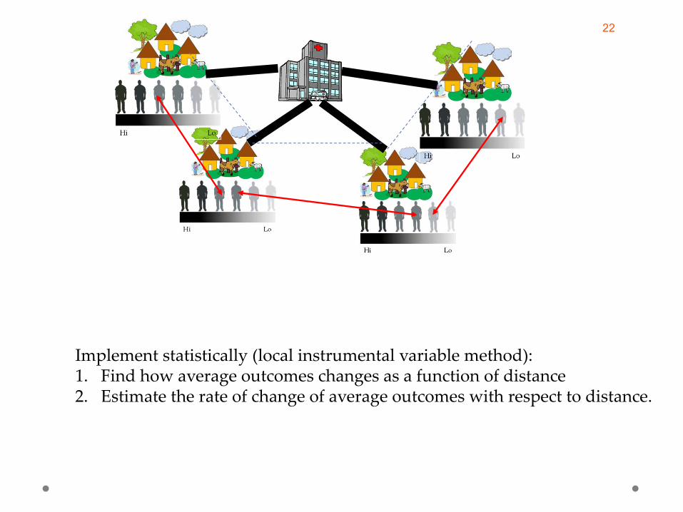
Implement statistically (local instrumental variable method):1. Find how average outcomes changes as a function of distance2. Estimate the rate of change of average outcomes with respect to distance.

22

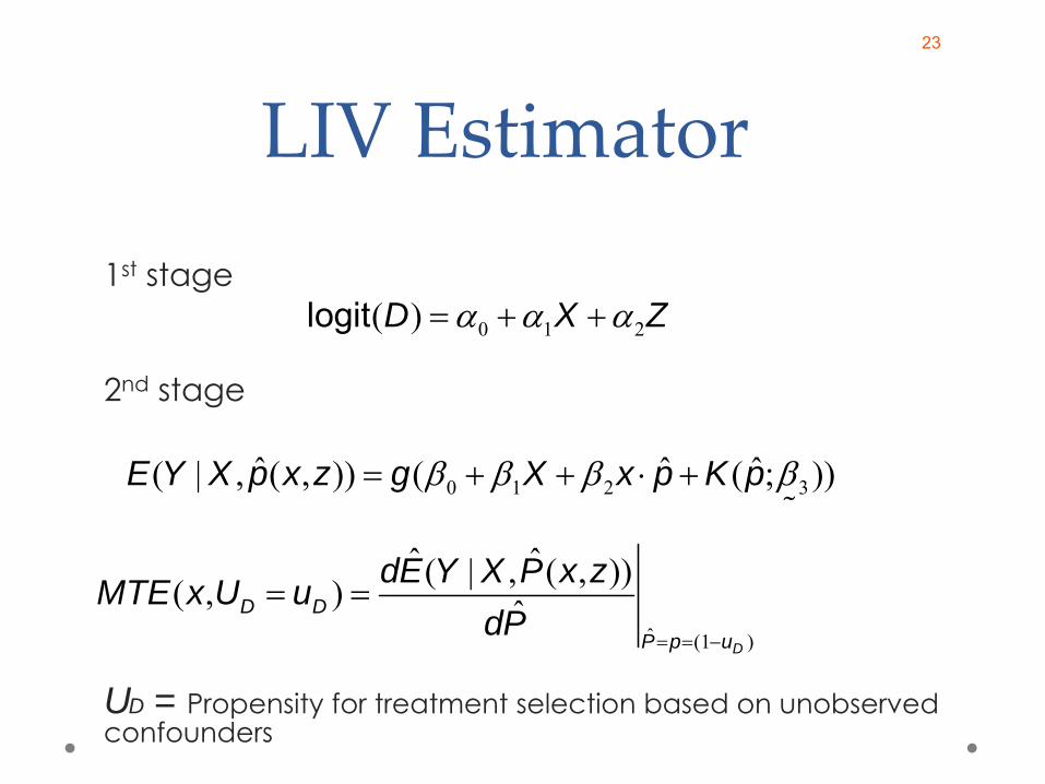
LIV Estimator1st stage

2nd stage

UD = Propensity for treatment selection based on unobserved confounders

0 1 2( )logit D X Z

0 1 2 3ˆ ˆ ˆ( | , ( , )) ( ( ; ))E Y X p x z g X x p K p

ˆ (1 )

ˆ ˆ( | , ( , ))( , ) ˆD

D D

P p u

dE Y X P x zMTE x U udP

23

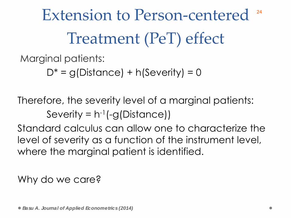
Extension to Person‐centered Treatment (PeT) effect

Marginal patients: D* = g(Distance) + h(Severity) = 0

Therefore, the severity level of a marginal patients:Severity = h-1(-g(Distance))

Standard calculus can allow one to characterize the level of severity as a function of the instrument level, where the marginal patient is identified.

Why do we care?

Basu A. Journal of Applied Econometrics (2014)

24


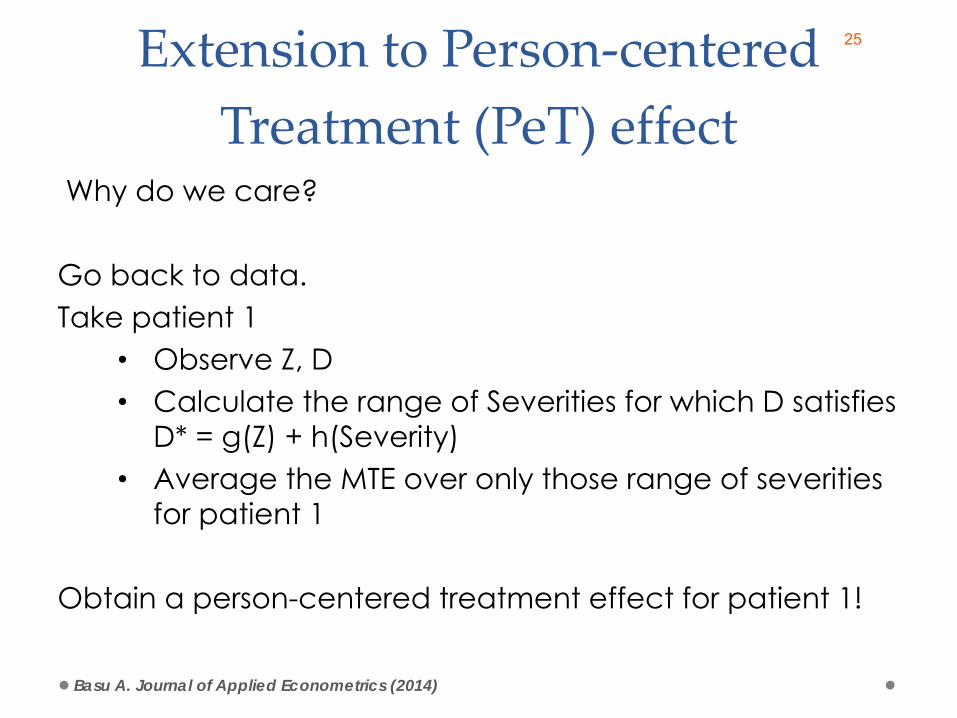
Why do we care?

Go back to data.Take patient 1

• Observe Z, D• Calculate the range of Severities for which D satisfies

D* = g(Z) + h(Severity) • Average the MTE over only those range of severities

for patient 1

Obtain a person-centered treatment effect for patient 1!


25


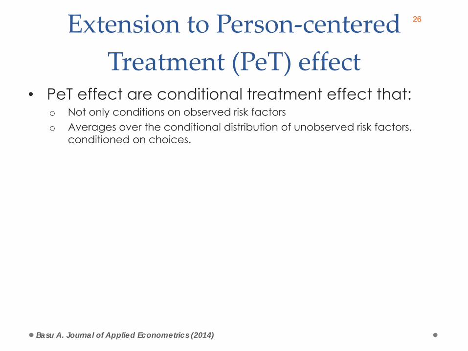
• PeT effect are conditional treatment effect that:o Not only conditions on observed risk factorso Averages over the conditional distribution of unobserved risk factors,

conditioned on choices.


26


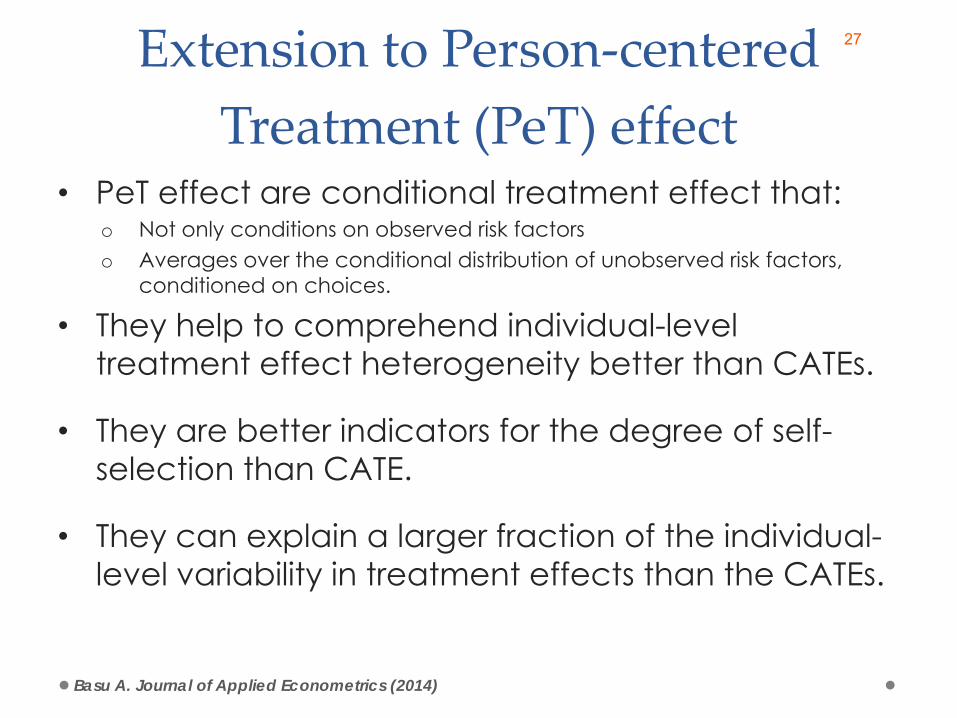
• PeT effect are conditional treatment effect that:o Not only conditions on observed risk factorso Averages over the conditional distribution of unobserved risk factors,

conditioned on choices.

• They help to comprehend individual-level treatment effect heterogeneity better than CATEs.

• They are better indicators for the degree of self-selection than CATE.

• They can explain a larger fraction of the individual-level variability in treatment effects than the CATEs.


27

Estimation of PeT effects• Basu A. Person-Centered Treatment (PeT) effects using

instrumental variables: An application to evaluating prostate cancer treatments. Journal of Applied Econometrics 2014; 29:671-691.

• Basu A. Person-centered treatment (PeT) effects: Individualized treatment effects with instrumental variables. Stata Journal In Press.

• -petiv- command in STATA

28

PeT Estimation Algorithm• Numerical integration: For each individual i:

o Draw 1000 deviates u~Uniform[min(P), max(P)]

o Compute and evaluate it by replacing P with each value of u.

o Compute D* = Φ-1(P)+Φ-1(1-u) also generating 1000 values for each individual.

o Compute PeT by averaging over values of u for which (D* > 0) if D=1, otherwise, by averaging over values of u for which (D* ≤ 0) if D=0.

• Estimated PeT effects provide us with individualized effects of treatment effects. Mean treatment effect parameters were also computed. Averaging PeTs over all observation gave ATE. Averaging PeTs over over D=1 or D=0 gave us TT and TUT respectively.

ˆ ˆ(.) /dg dp

ˆ ˆ(.) /dg dp

29

Empirical ExampleDoes transfer to intensive care units reduce mortality for

deteriorating ward patients?

30

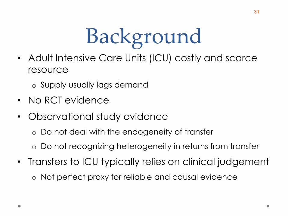
Background• Adult Intensive Care Units (ICU) costly and scarce

resourceo Supply usually lags demand

• No RCT evidence• Observational study evidence

o Do not deal with the endogeneity of transfer

o Do not recognizing heterogeneity in returns from transfer

• Transfers to ICU typically relies on clinical judgemento Not perfect proxy for reliable and causal evidence

31

Our Study• Exploit natural variation in ICU transfer according to

ICU bed availability for deteriorating ward patients in the UK

• The (SPOT)light Study (N = 15,158)o Prospective cohort study of the deteriorating ward patients

referred for assessment for ICU transfer

o Hospitals were eligible for inclusion if they participated in the ICNARC Case Mix Programme

o Patients recruited between Nov 1, 2010 - Dec 31, 2011 from 49 UK NHS hospitals

o A variety of exclusion conditions were applied to identify deteriorating ward patients who are equipoised to be transferred to ICU

32

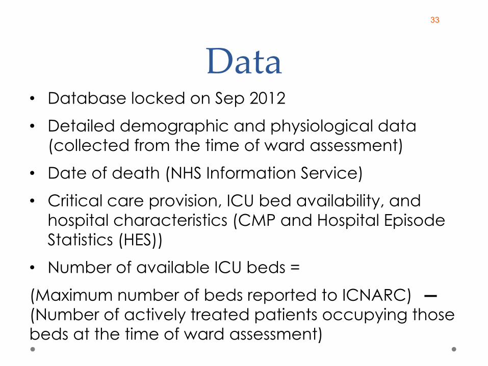
Data• Database locked on Sep 2012• Detailed demographic and physiological data

(collected from the time of ward assessment)• Date of death (NHS Information Service)• Critical care provision, ICU bed availability, and

hospital characteristics (CMP and Hospital Episode Statistics (HES))

• Number of available ICU beds = (Maximum number of beds reported to ICNARC) ―(Number of actively treated patients occupying those beds at the time of ward assessment)

33

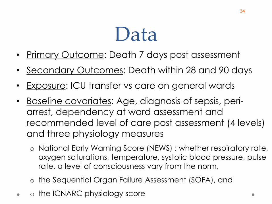
Data• Primary Outcome: Death 7 days post assessment• Secondary Outcomes: Death within 28 and 90 days• Exposure: ICU transfer vs care on general wards• Baseline covariates: Age, diagnosis of sepsis, peri-

arrest, dependency at ward assessment and recommended level of care post assessment (4 levels) and three physiology measureso National Early Warning Score (NEWS) : whether respiratory rate,

oxygen saturations, temperature, systolic blood pressure, pulse rate, a level of consciousness vary from the norm,

o the Sequential Organ Failure Assessment (SOFA), and

o the ICNARC physiology score

34

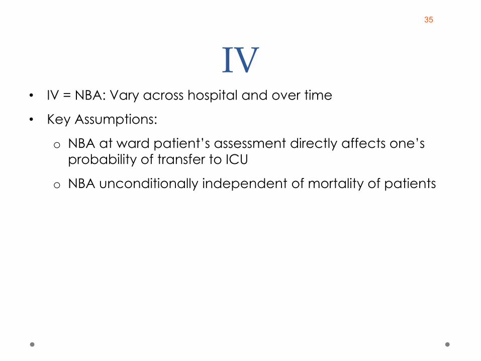
IV• IV = NBA: Vary across hospital and over time

• Key Assumptions:

o NBA at ward patient’s assessment directly affects one’s probability of transfer to ICU

o NBA unconditionally independent of mortality of patients

35

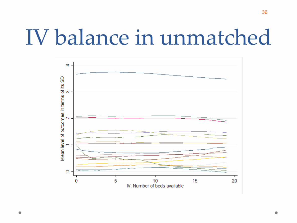
IV balance in unmatched36

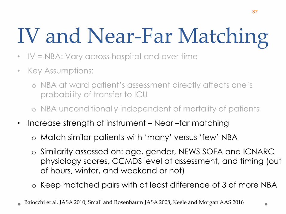
IV and Near‐Far Matching• IV = NBA: Vary across hospital and over time

• Key Assumptions:

o NBA at ward patient’s assessment directly affects one’s probability of transfer to ICU

o NBA unconditionally independent of mortality of patients

• Increase strength of instrument – Near –far matching

o Match similar patients with ‘many’ versus ‘few’ NBA

o Similarity assessed on: age, gender, NEWS SOFA and ICNARC physiology scores, CCMDS level at assessment, and timing (out of hours, winter, and weekend or not)

o Keep matched pairs with at least difference of 3 of more NBA

Baiocchi et al. JASA 2010; Small and Rosenbaum JASA 2008; Keele and Morgan AAS 2016

37

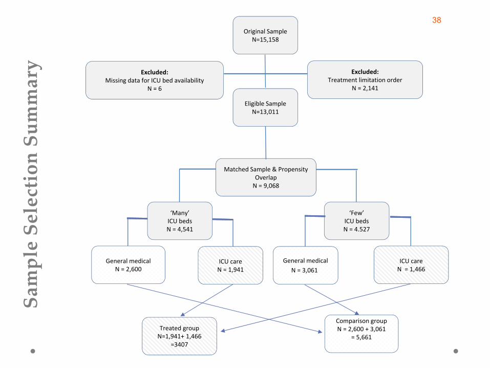
ICU care N = 1,941

General medical N = 2,600

‘Many’ ICU beds N = 4,541

‘Few’ ICU beds N = 4.527

Original SampleN=15,158

Eligible SampleN=13,011

Matched Sample & Propensity OverlapN = 9,068

Excluded:Treatment limitation order

N = 2,141

Excluded:Missing data for ICU bed availability

N = 6

General medical N = 3,061

ICU care N = 1,466

Treated groupN=1,941+ 1,466

=3407

Comparison groupN = 2,600 + 3,061

= 5,661

Sample Selection Summary

38

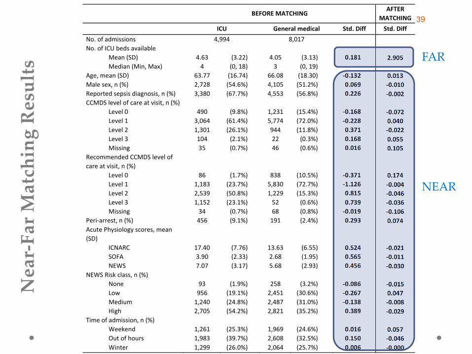
BEFORE MATCHING AFTER

MATCHING ICU General medical Std. Diff Std. Diff No. of admissions 4,994 8,017 No. of ICU beds available Mean (SD) 4.63 (3.22) 4.05 (3.13) 0.181 2.905 Median (Min, Max) 4 (0, 18) 3 (0, 19) Age, mean (SD) 63.77 (16.74) 66.08 (18.30) ‐0.132 0.013 Male sex, n (%) 2,728 (54.6%) 4,105 (51.2%) 0.069 ‐0.010 Reported sepsis diagnosis, n (%) 3,380 (67.7%) 4,553 (56.8%) 0.226 ‐0.002 CCMDS level of care at visit, n (%) Level 0 490 (9.8%) 1,231 (15.4%) ‐0.168 ‐0.072 Level 1 3,064 (61.4%) 5,774 (72.0%) ‐0.228 0.040

Level 2 1,301 (26.1%) 944 (11.8%) 0.371 ‐0.022 Level 3 104 (2.1%) 22 (0.3%) 0.168 0.055 Missing 35 (0.7%) 46 (0.6%) 0.016 0.105

Recommended CCMDS level of care at visit, n (%)

Level 0 86 (1.7%) 838 (10.5%) ‐0.371 0.174 Level 1 1,183 (23.7%) 5,830 (72.7%) ‐1.126 ‐0.004 Level 2 2,539 (50.8%) 1,229 (15.3%) 0.815 ‐0.046 Level 3 1,152 (23.1%) 52 (0.6%) 0.739 ‐0.036 Missing 34 (0.7%) 68 (0.8%) ‐0.019 ‐0.106

Peri‐arrest, n (%) 456 (9.1%) 191 (2.4%) 0.293 0.074 Acute Physiology scores, mean (SD)

ICNARC 17.40 (7.76) 13.63 (6.55) 0.524 ‐0.021 SOFA 3.90 (2.33) 2.68 (1.95) 0.565 ‐0.011 NEWS 7.07 (3.17) 5.68 (2.93) 0.456 ‐0.030 NEWS Risk class, n (%) None 93 (1.9%) 258 (3.2%) ‐0.086 ‐0.015 Low 956 (19.1%) 2,451 (30.6%) ‐0.267 0.047 Medium 1,240 (24.8%) 2,487 (31.0%) ‐0.138 ‐0.008 High 2,705 (54.2%) 2,821 (35.2%) 0.389 ‐0.029 Time of admission, n (%) Weekend 1,261 (25.3%) 1,969 (24.6%) 0.016 0.057 Out of hours 1,983 (39.7%) 2,608 (32.5%) 0.150 ‐0.046 Winter 1,299 (26.0%) 2,064 (25.7%) 0.006 ‐0.000

Near‐Far M

atching Results

FAR

NEAR

39

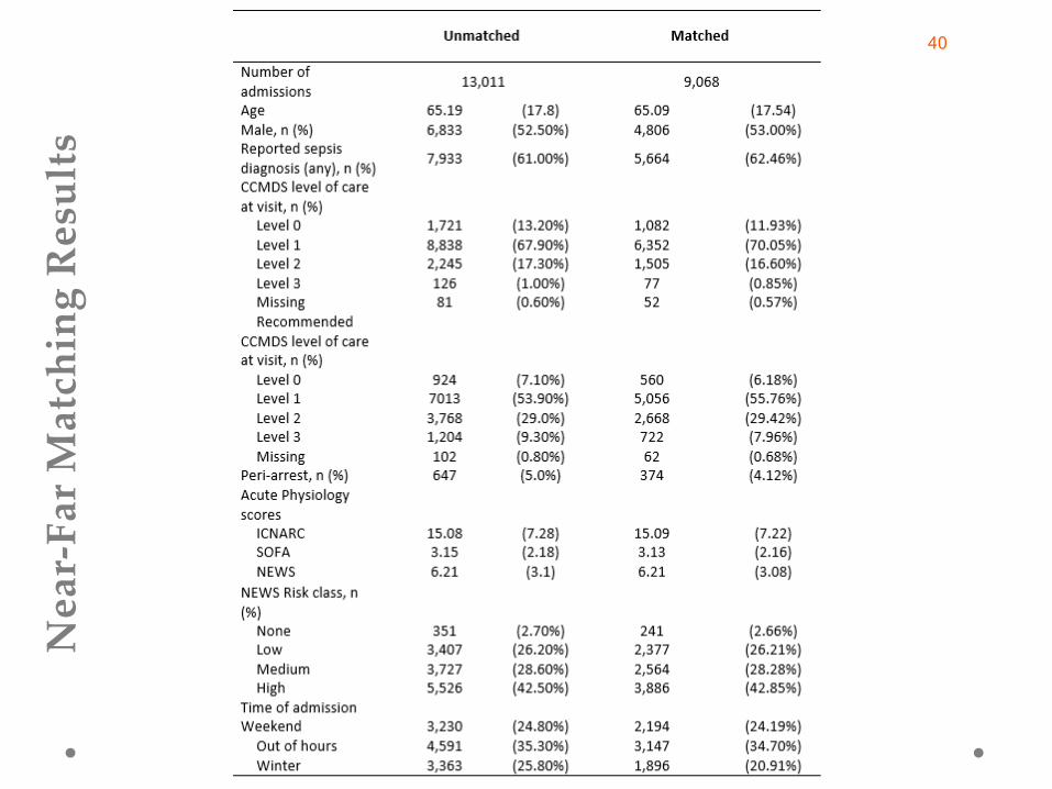
Near‐Far M

atching Results

40

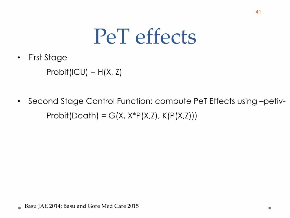
PeT effects• First Stage

Probit(ICU) = H(X, Z)

• Second Stage Control Function: compute PeT Effects using –petiv-

Probit(Death) = G(X, X*P(X,Z), K(P(X,Z)))

Basu JAE 2014; Basu and Gore Med Care 2015

41

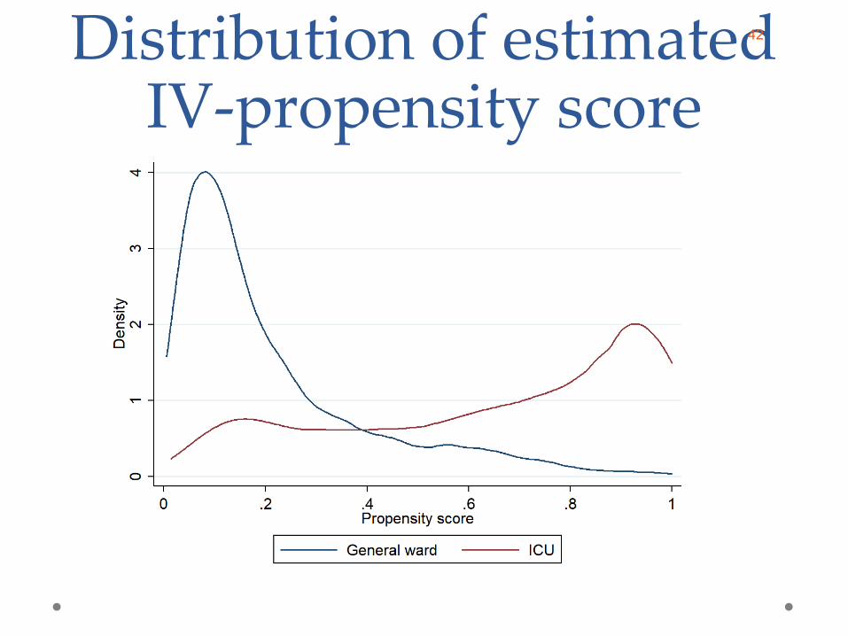
Distribution of estimated IV‐propensity score

42

ReferencesBasu A, Meltzer D. Value of information on preference heterogeneity and individualized care. Medical Decision Making 2007; 27(2):112-127.

Basu A, Heckman J, Navarro-Lozano S, et al. Use of instrumental variables in the presence of heterogeneity and self-selection: An application to treatments of breast cancer patients. Health Econ 2007; 16(11): 1133 -1157.

Basu A. 2009. Individualization at the heart of comparative effectiveness research: The time for i-CER has come. Medical Decision Making, 29(6): N9-N11.

Basu A, Jena AB, Philipson TJ. The impact of comparative effectiveness research on health and health care spending. J Health Econ. 2011;30(4):695-706.

Basu A. Economics of individualization in comparative effectiveness research and a basis for a patient-centered health care. J Health Econ. 2011; 30(3):549-559.

Basu A. Person-Centered Treatment (PeT) effects using instrumental variables: An application to evaluating prostate cancer treatments. Journal of Applied Econometrics (In Press).

Heckman JJ, Vytlacil EJ. Local instrumental variables and latent variable models for identifying and bounding treatment effects. Proc Nat Acad Sci 1999; 96(8): 4730-34

Heckman JJ, Urzua S, Vytlacil E. Understanding instrumental variables in models with essential heterogeneity. Rev Econ Stat 2006; 88(3): 389-432.

Kaplan S, Billimek J, Sorkin D, Ngo-Metzger Q, Greenfield S. Who Can Respond to Treatment?: Identifying Patient Characteristics Related to Heterogeneity of Treatment Effects. Medical Care 2010; 48(6): S9-S16

51

Health & Medicine

Does transfer to intensive care units reduce mortality for deteriorating ward patients? Estimating Person-centered Treatment (PeT) effects using instrumental variables