Gender Wage Differentials in the Finnish Labour Market

179GENDER WAGEDIFFERENTIALSIN THE FINNISH

LABOURMARKET

Juhana Vartiainen

PALKANSAAJIEN TUTKIMUSLAITOS •• TYÖPAPEREITALABOUR INSTITUTE FOR ECONOMIC RESEARCH •• DISCUSSION PAPERS

Helsinki 2002

179

GENDER WAGEDIFFERENTIALSIN THE FINNISHLABOURMARKET

Juhana Vartiainen

ISBN 952−5071−67−7ISSN 1457−2923

Gender wage differentials in the Finnish labourmarket∗

Juhana Vartiainen

March 4, 2002

Abstract

A comprehensive analysis of the gender wage differential among Finnish full timeemployees is reported. Oaxaca decompositions show that the the overall wage gap ofabout 21.5 per cent cannot be accounted for by individual characteristics, since age andeducational qualifications are rather similar for men and women. When industry and occu-pational qualifications are included in the regressor matrix, the unexplained part shrinks toabout 50 per cent of the gross differential. An even larger part of the gross differential canbe explained in sector-specific analyses with a dense set of occupational dummies. In aless standard part of the analysis, we characterise the distribution of the unexplained wagegap across the variable space. It turns out the women with a high wage predictor, that is,women with good educational qualifications in well-remunerated occupations, drag themost behind their male colleagues endowed with similar characteristics. JEL numbersJ31, J70, J71.

Tiivistelmä

Sukupuolten palkkaero on kokopäiväisten palkansaajien parissa noin 20 prosenttia elinaiset ansaitsevat osapuilleen neljä viidesosaa miesten ansioista. Artikkelissa analysoidaantaloustieteen keinoin tätä palkkaeroa. Se on yhteenveto laajemmasta tutkimusraportista

∗This paper summarises some results of the project “Measuring and monitoring gender wage differentials inthe Finnish labour market”, commissioned by the Ministry of Social Affairs and Health and carried out by theauthor. The objective of the project was to present a comprehensive survey of the gender wage differential in theFinnish labour market as well as to suggest statistical procedures that could be used for a more regular monitoringof the gender wage gap. A longer report in Finnish (55 pages of main text plus a 249-page statistical annex) isavailable (see Vartiainen (2001)). In that report, a more comprehesive set of sector-specific statistics is presented.I am grateful to Equality Ombudsman Pirkko Mäkinen and Research Officer Anita Haataja for sponsoring andsupporting this research. I am grateful to Reija Lilja for useful comments. I also want to thank the variousemployers’ organisations who made possible the use of their sector-specific wage databases, as well as StatisticsFinland, whose co-operation has been primordial. Any errors or weaknesses are my own, of course. Author’saffiliation and e-mail: Labour Institute for Economic Research, Helsinki. [email protected]

3

(Vartiainen 2001), jonka pyrkimyksenä oli kartoittaa kattavasti sukupuolten palkkaeroaSuomessa sekä ehdottaa tilastointi- ja seurantatapoja, jolla tätä eroa voitaisiin vastaisuu-dessa seurata. Tulokset osoittavat, että mainitusta 20 prosentin palkkaerosta selittyy poisnoin puolet, jos selittäjinä käytetään henkilökohtaisia muuttujia sekä toimialoille ja am-mattiryhmiin valikoitumista. Sukupuolten välillä ei ole merkittävää eroa iässä ja koulutuk-sessa, joten palkkaeron selittyvä osa perustuu toimiala- ja ammattiryhmävalikoitumiseen.Samanlainen hajoitelma lasketaan myös talouden viidelle sektorille (palvelutyönantajat,teollisuuden tuntipalkkaiset, teollisuuden kuukausipalkkaiset, kunnat, valtio) erikseen.Tulokset osoittavat, että julkisyhteisöjen parissa toteutuu pitkälti “sama palkka samastatyöstä” -periaate, ja lopullinen palkkaero syntyy lähes kokonaan naisten ja miesten am-mattiryhmävalikoitumisen kautta.

Teollisuuden piirissä ammatteihin valikoituminen ei ole yhtä merkittävä sukupuoltenpalkkaeron taustatekijä, mutta iän palkkaa nostava vaikutus on naisilla selvästi vähäisempikuin miehillä.

Artikkelissa tarkastellaan myös selittymättömän palkkaeron jakautumista eri palkkata-soille. Selittymätön palkkakaula on suurempi korkean palkkatason tehtävissä kuin matala-palkkatehtävissä. Sukupuolten ammatillista segregoitumista kuvaavat indeksit osoittavatsegregoitumisen hidasta heikkenimistä.

4

Contents

1 Introduction 6

2 Data 6

3 The Oaxaca decomposition 73.1 Definition . . . . . . . . . . . . . . . . . . . . . . . . . . . . . . . . . . . . 73.2 Results for all employees . . . . . . . . . . . . . . . . . . . . . . . . . . . . 93.3 Results for specific sectors . . . . . . . . . . . . . . . . . . . . . . . . . . .12

4 The distribution of the unexplained gap 16

5 Educational groups 20

6 A note on segregation 21

7 Concluding remarks 22

5

1 Introduction

This paper presents the most important stylised facts about the gender wage differential in theFinnish economy. We characterise the differential in two ways. The first is a standard one: weuse an Oaxaca decomposition (see Oaxaca (1973)) of the log of the monthly wage and presentthe decomposition results. The results are presented both with and without an occupationaldummy variable, and, in both cases, using both the male and female parameter estimates as thereference structure. The estimates are based on a 20 per cent sample of the Earnings Database(“palkkarakennetilasto”) produced and maintained by Statistics Finland. This database coversalmost the entire salaried workforce of the economy. Our study concerns the wages of full-timeworkers and employees.

The first decompositions exploit the entire sample. The data are then decomposed into sub-sets: service sector, manufacturing (salaried employees and wage earners paid by the hour aretreated separately), local government and central government. Oaxaca decomposition resultsare presented for these subsets as well.

The second set of results is more original. The Oaxaca decomposition reveals the averageunexplained wage gap between sexes but nothing about its distribution. Yet, from the point ofview of society’s welfare and gender equality, it is quite interesting to ask how that unexplainedwage gap is distributed in different parts of the variable space. Most studies of the wagedifferential do not appreciate this point, with the exception of Stephen Jenkins who has in aninteresting way applied the ideas familiar from the theory of income distribution to the studyof group differentials (see Jenkins (1994)). However, since the aim of this paper is to get outthe most important stylised facts, we adopt a far simpler procedure, described in more detailin section 4.

2 Data

We exploit the Earnings Structure Database maintained by Statistics Finland. It is based on acompilation of wage registries kept by various employer organisations and comprises about 1.3million wage-earners. The variables include a detailed breakdown of earnings variables plusbackground variables like age and schooling, together with industrial sector and occupationaldummies. We sampled a 20 per cent subset of that database, so that the probability of selectioninto the sample was proportional to the sampling weight used by Statistics Finland; by thesemeans, we sought to emulate simple random sampling as fully as possible.

The variable of interest ismonthly wage incomeas computed by Statistics Finland. Thatvariable has been computed by dividing all wage and salary incomes of the individual byhis/her total working hours, both measured under a month. The aim has been to include allsuch wage items that have some continuity: the base wage, extras and bonuses based on work-ing conditions, eventual extra pay due to overtime and the value of perks. Similarly, the de-nominator was an estimated total labour input as measured in time units.

6

We excluded all part-time employees from our analysis. This was motivated by the willto compare men and women who would be as similar as possible. The inclusion of part-timework would point the way to another kind of analysis in which the differential labour supplydecisions of men and women would play a more central role.

3 The Oaxaca decomposition

3.1 Definition

The Oaxaca decomposition was presented in (Oaxaca, 1973), and we follow his procedure. Ifthe male and female geometric mean wages are denoted byWM andW F , we can decomposethe log-differential of geometric means as follows:

∆ ≡ log(WM/W F ) = (log(WM)− logW 0F ) + (log(W 0F )− logW F ), (1)

in which we denote byW 0F a hypothetical distortion-free or discrimination-free mean wagefor women. Furthermore, we can summarise the variation in the male and female wage crosssection samples by using the following commonplace statistical models:

wi,m = X iβM + εi (2)

and

wj,f = XjβF + εj (3)

in whichwi,m is the log wage of mani andwj,f is the log wage of womanj, βM andβF arethe coefficients that determine the effect of characteristics on pay and theX i andXj are thevectors of characteristics of mani and womanj. Taking the arithmetic average of equations(2) and (3), the stochasticε-terms drop away. Designating arithmetic mean by an underlinedvariable, we have

wm = XMβM (4)

and

wf = XFβF , (5)

which simply says that mean wages are predicted by using mean characteristics. Sincew isthe mean of the log, it is the log of the geometric meanW . We can then plug equations (4) and(5) into (1) to obtain:

∆ = (XM −XF )βM +XF (βM − βF ). (6)

7

Thus, the gross differential∆ is decomposed into the effect of differences in average char-acteristics (the first term) and the effect of different treatment (or different “pricing”) of char-acteristics. In this paper, we shall speak of the contribution of different characteristics on theone hand and of the unexplained differential or “differential pricing” effect on the other.

The literature often speaks roughly of the latter part as “discrimination”, but this is a du-bious usage of words. The unexplained part contains the effects of all those variables that arenot part of theX-matrix; economic theory suggests many ways in which unobserved variablesmay be differently distributed across men and women and may thereby contribute to the wagedifferential as well. If there is outright discrimination in wage-setting, it is probably a part ofthe unexplained component.

In the above decomposition, we implicitly chose the male coefficient vector as a referencestructure with which we evaluated (i.e. “priced”) the contribution of the differences in char-acteristics. We could equally well choose the female wage structure and get the analogousdecomposition

∆ = (XF −XM)βF +XM(βF − βM). (7)

In the subsequent literature, it has been emphasised that there is in general no unambiguou-osly best way to choose the reference wage structure (this is really an index number problem).Ideally, if we knew a “right”, discrimination-free structureβ, we should use it to evaluate theeffect of differences in characteristics. Some authors use the coefficients estimated from thepooled sample (without female dummy) as the reference structure.

More generally, the reference structure can be chosen as a matrix weighted average of themale and femaleβ-vectors (see Oaxaca and Ransom (1994)). The choice of the weightingmatrix should be guided by economic theory, but the literature on this issue is still quite rudi-mentary. We have therefore chosen simply to present the computations using both male andfemale coefficients as reference. The advantage of this procedure is that it enables a clearinterpretation: using the male (female) structure as reference and computing the effect of dif-ferent characteristics yields an answer to the question “how much would remain of the grossdifferential if women (men) were treated as men (women) with similar characateristics?”.

Note that the above decompositions can be expanded to yield the contributions of eachsingle regressor: how much of the gross differential is due to the gender difference in meansof the regressor and how much is due to differential pricing of the regressor. This interpre-tation runs into trouble when we include categorical variables in the regressor matrixX. Asis shown in Oaxaca and Ransom (1999), the presence of categorical variables implies that theunexplained part (i.e. the “differential pricing”) part of each categorical variable cannot beuniquely determined. This is intuitively clear, since the regression of wages on categoricalvariables implies a choice of a reference group, and the results of the Oaxaca decompositionare not independent of this choice. The combined “differential pricing” contribution of all thewithin-cell unexplained gaps can be uniquely computed, however, and we shall report that inour tables.

8

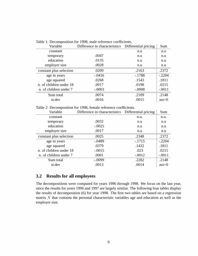
Table 1: Decomposition for 1998, male reference coefficients.Variable Difference in characteristics Differential pricingSumconstant n.u n.u

temporary .0047 n.u n.ueducation .0135 n.u n.u

employer size .0028 n.u n.u

constant plus selection .0209 .2163 .2372age in years -.0416 -.1788 -.2204age squared .0268 .1543 .1811

n. of children under 18 .0017 .0198 .0215n. of children under 7 -.0003 -.0008 -.0011

Sum total .0074 .2109 .2148st.dev .0016 .0015 ass=0

Table 2: Decomposition for 1998, female reference coefficients.Variable Difference in characteristics Differential pricingSumconstant n.u. n.u.

temporary .0032 n.u n.ueducation -.0025 n.u n.u



n. of children under 18 -.0015 .023 .0215n. of children under 7 .0001 -.0012 -.0011

Sum total -.0099 .2282 .2148st.dev .0013 .0014 ass=0

3.2 Results for all employees

The decompositions were computed for years 1996 through 1998. We focus on the last year,since the results for years 1996 and 1997 are largely similar. The following four tables displaythe results of decomposition (6) for year 1998. The first two tables are based on a regressionmatrixX that contains the personal characteristic variables age and education as well as theemployer size.

9

The tables are read as follows. The cell at the low-end right-end corner (at the intersectionof row “Sum total” and column “Sum” tells the gross log wage differential (21.48 in Table 1,for example). The two entries on the same row display the two terms of decomposition (6); thefirst one is the effect of differences in characteristics and the second one is the unexplained ordifferential pricing component. The other rows above that final row tell the same informationfor different variables. The first group of variables (above the first horizontal double line)is the group of categorical variables. For those ones, one can only compute the effect of thedifference in means in an unambiguous way; the pricing effect is reported as the aggregate sumof the within-cell unexplained gaps (the abbreviation “n.u” stands for “not unique”). This isreported on the row “constant plus selection”. The second group of variables are the continuousones: age, age squared and the number of children. Finally, the row “Sum total” adds up allthe contributions.

Tables 1 and 2 make it clear that personal characteristics plus firm size do not go far inexplaining the wage differential. Of the overall differential of 21.5 percentage points, almostnothing is explained by differences in individual characteristics and employer size. Almostall of the wage differential is due to a constant term that we cannot allocate to any specificcategorical variable.

The next two tables 3 and 4 show the analogous results when an occupational variable1

plus a sector variable2 (“industry”) are added to the regressor matrix. We see now that abouthalf of the gross wage differential can be accounted for by different endowments when malecoefficients are used, and about one third when female coefficients are used. The tables showthat the “industry” variable and the “occupation” variable together generate the explained partof about 10 percentage points.

1This is the “isco” -variable produced and used by Statistics Finland.2The “nace” variable of Statistics Finland.

10

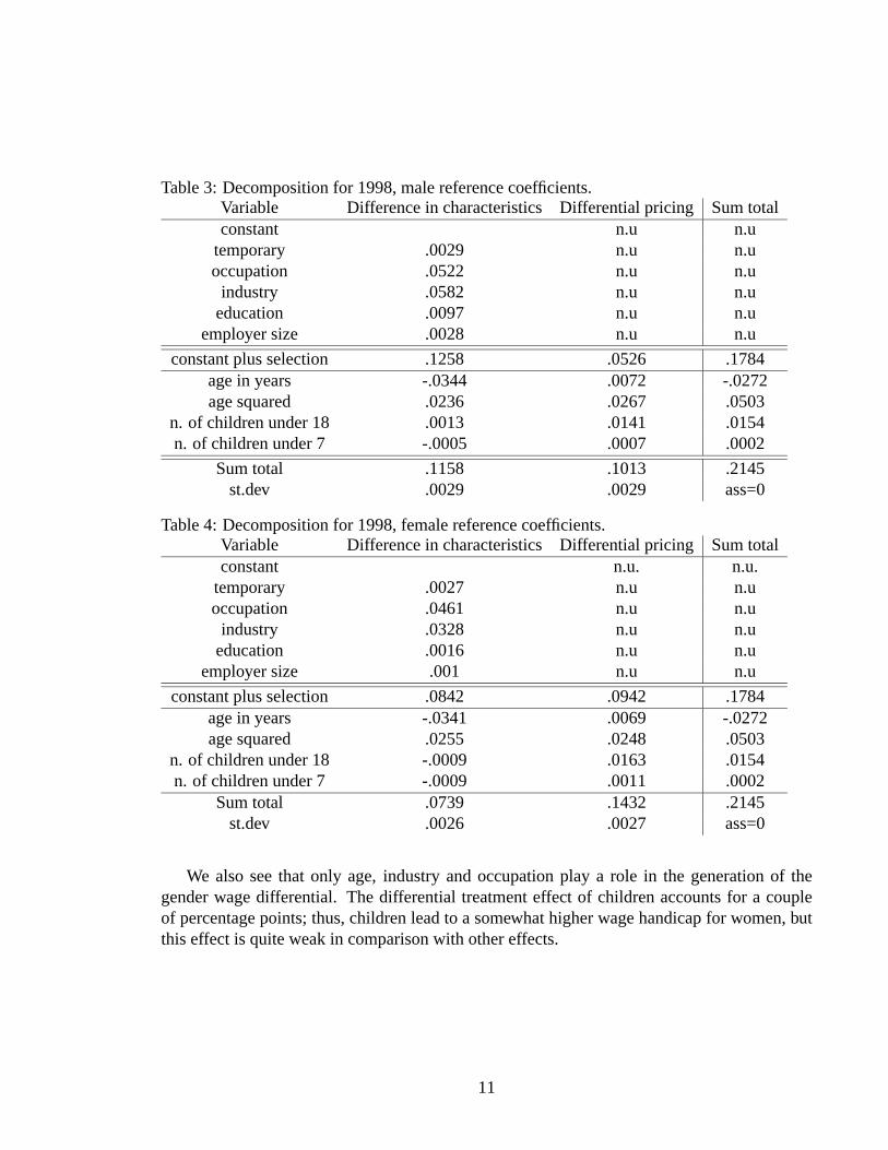
Table 3: Decomposition for 1998, male reference coefficients.Variable Difference in characteristics Differential pricingSum totalconstant n.u n.u

temporary .0029 n.u n.uoccupation .0522 n.u n.uindustry .0582 n.u n.u

education .0097 n.u n.uemployer size .0028 n.u n.u

constant plus selection .1258 .0526 .1784age in years -.0344 .0072 -.0272age squared .0236 .0267 .0503

n. of children under 18 .0013 .0141 .0154n. of children under 7 -.0005 .0007 .0002


Table 4: Decomposition for 1998, female reference coefficients.Variable Difference in characteristics Differential pricingSum totalconstant n.u. n.u.

temporary .0027 n.u n.uoccupation .0461 n.u n.uindustry .0328 n.u n.u

education .0016 n.u n.uemployer size .001 n.u n.u

constant plus selection .0842 .0942 .1784age in years -.0341 .0069 -.0272age squared .0255 .0248 .0503

n. of children under 18 -.0009 .0163 .0154n. of children under 7 -.0009 .0011 .0002


We also see that only age, industry and occupation play a role in the generation of thegender wage differential. The differential treatment effect of children accounts for a coupleof percentage points; thus, children lead to a somewhat higher wage handicap for women, butthis effect is quite weak in comparison with other effects.

11

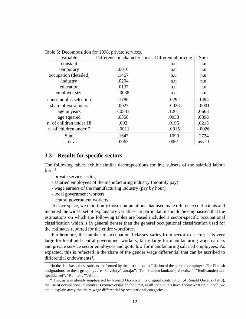
Table 5: Decomposition for 1998, private services.Variable Difference in characteristics Differential pricingSumconstant n.u n.u

temporary .0016 n.u n.uoccupation (detailed) .1467 n.u n.u

industry .0204 n.u n.ueducation .0137 n.u n.u

employer size -.0038 n.u n.u

constant plus selection .1786 -.0292 .1494share of extra hours .0027 -.0028 -.0001

age in years -.0533 .1201 .0668age squared .0358 .0038 .0396


Sum .1647 .1099 .2724st.dev .0063 .0061 ass=0

3.3 Results for specific sectors

The following tables exhibit similar decompositions for five subsets of the salaried labourforce3:

- private service sector;- salaried employees of the manufacturing industry (monthly pay)- wage earners of the manufacturing industry (pay by hour)- local government workers- central government workers.To save space, we report only those computations that used male reference coefficients and

included the widest set of explanatory variables. In particular, it should be emphasised that theestimations on which the following tables are based included a sector-specific occupationalclassification which is in general denser than the general occupational classification used forthe estimates reported for the entire workforce.

Furthermore, the number of occupational classes varies from sector to sector; it is verylarge for local and central government workers, fairly large for manufacturing wage-earnersand private service sector employees and quite low for manufacturing salaried employees. Asexpected, this is reflected in the share of the gender wage differential that can be ascribed todifferential endowments4.

3In the data base, these subsets are formed by the institutional affiliation of the person’s employer. The Finnishdesignations for these groupings are “Palvelutyönantajat”, “Teollisuuden kuukausipalkkaiset”, “Teollisuuden tun-tipalkkaiset”, “Kunnat”, “Valtio”.

4Thus, as was already emphasised by Ronald Oaxaca in his original contribution of Ronald Oaxaca (1973),the use of occupational dummies is controversial. In the limit, as all individuals have a somewhat unique job, wecould explain away the entire wage differential by occupational categories.

12

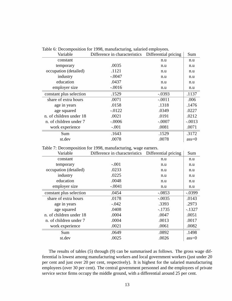
Table 6: Decomposition for 1998, manufacturing, salaried employees.Variable Difference in characteristics Differential pricingSumconstant n.u n.u

temporary .0035 n.u n.uoccupation (detailed) .1121 n.u n.u

industry -.0047 n.u n.ueducation .0437 n.u n.u


constant plus selection .1529 -.0393 .1137share of extra hours .0071 -.0011 .006

age in years .0158 .1318 .1476age squared -.0122 .0349 .0227


work experience -.001 .0081 .0071

Sum .1643 .1529 .3172st.dev .0078 .0078 ass=0

Table 7: Decomposition for 1998, manufacturing, wage earners.Variable Difference in characteristics Differential pricingSumconstant n.u n.u

temporary -.001 n.u n.uoccupation (detailed) .0233 n.u n.u



constant plus selection .0454 -.0853 -.0399share of extra hours .0178 -.0035 .0143

age in years -.042 .3393 .2973age squared .0408 -.1735 -.1327

n. of children under 18 .0004 .0047 .0051n. of children under 7 .0004 .0013 .0017

work experience .0021 .0061 .0082

Sum .0649 .0892 .1498st.dev .0025 .0026 ass=0

The results of tables (5) through (9) can be summarised as follows. The gross wage dif-ferential is lowest among manufacturing workers and local government workers (just under 20per cent and just over 20 per cent, respectively). It is highest for the salaried manufacturingemployees (over 30 per cent). The central government personnel and the employees of privateservice sector firms occupy the middle ground, with a differential around 25 per cent.

13

In these sector-specific computations, we have had to discard some observations that be-long to the smallest and most segregated occupational categories, since no reliable statisticalinference is possible if a cell contains only a couple of female or a couple of male obser-vations5. This truncation of the data has a different effect in different sectors. Deleting thesmallest and most segregated occupational categories leads to a large drop in the gender differ-ential of manufacturing wage-earners; as is apparent from table 7, the gross wage differential isas low as 15 per cent. Thus, the most segregated occupational categories tend to be populatedby high-earning males and low-earning females. Among the local government workers, thistruncation has the opposite effect of increasing the gross wage differential. Small and segre-gated occupational categories tend there to include female with high earnings and males withlow earnings.

The tables indicate that segregated occupational categorisation explains away most of thewage differential in the case of local and central government employees. In both cases, 80 to90 per cent of the gross differential is explained by differences in the means of the regressors,and segregation into different occupations is in turn responsible for about 4/5 of that effect(see the entry at the intersection of row “occupational category” and column “Difference incharacteristics” in tables 8 and 9: it is of the order of 15 percentage points in both sectors).The effect of differential treatment of age is quite limited.

The picture is somewhat different amongst the manufacturing industries employees andworkers. There, the share of the gross wage differential that can be explained away by differ-ent characteristics is in general lower, about half of the gross differential for salaried employeesand about a third of the gross differential for workers. A closer look at tables 6 and 7 revealsthat the effect of differential selection into occupational categories is much lower in manufac-turing than in the public sector ; it only contributes a couple of percentage points among wageearners and about 10 percentage points among salaried employees. The effect of differentialtreatment of age, by contrast, is an important factor: by itself, it creates an unexplained wagedifferential of about 16 percentage points in both subsets of manufacturing personnel. Notealso that the sum of unexplained mean gaps (see the entry at the intersection of row “constantplus selection” and column “Differential pricing” in tables 6 and 7) is negative. Thus, withinoccupational categories, manufacturing firms tend to pay more or less the same to young peo-ple, but the accruing of age leads to a widening gap between senior males and senior females.

Finally, for the employees of private service sector firms (see table 5) , the occupationalvariable is also quite important: segregated selection into occupations generates a wage differ-ential of almost 15 percentage points. Since differential age treatment plays an important roleas well, the computation ends up with a substantial gross differential of 27 percentage points,of which roughly 16 percentage points are explained by the regressors, mostly occupationalselection.

To sum up, the public sector seems prima facie to exemplify the principle of “similar payfor similar work”, since the remaining unexplained differential is quite low. Or, to put it inanother way, aspirations towards a lower gross differential should focus on the adequacy and

5We have required that an occupational category cell have at least 5 observations.

14

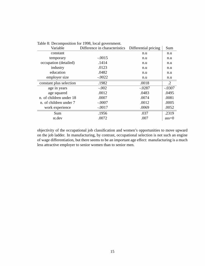
Table 8: Decomposition for 1998, local government.Variable Difference in characteristics Differential pricingSumconstant n.u n.u





n. of children under 18 .0007 .0074 .0081n. of children under 7 -.0007 .0012 .0005

work experience -.0017 .0069 .0052

Sum .1956 .037 .2319st.dev .0072 .007 ass=0

objectivity of the occupational job classification and women’s opportunities to move upwardon the job ladder. In manufacturing, by contrast, occupational selection is not such an engineof wage differentiation, but there seems to be an important age effect: manufacturing is a muchless attractive employer to senior women than to senior men.

15

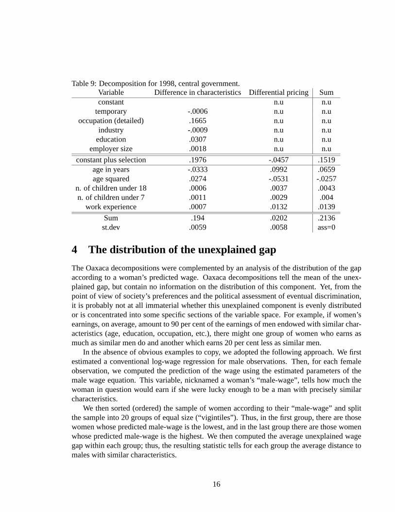
Table 9: Decomposition for 1998, central government.Variable Difference in characteristics Differential pricingSumconstant n.u n.u


industry -.0009 n.u n.ueducation .0307 n.u n.u


constant plus selection .1976 -.0457 .1519age in years -.0333 .0992 .0659age squared .0274 -.0531 -.0257

n. of children under 18 .0006 .0037 .0043n. of children under 7 .0011 .0029 .004

work experience .0007 .0132 .0139

Sum .194 .0202 .2136st.dev .0059 .0058 ass=0

4 The distribution of the unexplained gap

The Oaxaca decompositions were complemented by an analysis of the distribution of the gapaccording to a woman’s predicted wage. Oaxaca decompositions tell the mean of the unex-plained gap, but contain no information on the distribution of this component. Yet, from thepoint of view of society’s preferences and the political assessment of eventual discrimination,it is probably not at all immaterial whether this unexplained component is evenly distributedor is concentrated into some specific sections of the variable space. For example, if women’searnings, on average, amount to 90 per cent of the earnings of men endowed with similar char-acteristics (age, education, occupation, etc.), there might one group of women who earns asmuch as similar men do and another which earns 20 per cent less as similar men.

In the absence of obvious examples to copy, we adopted the following approach. We firstestimated a conventional log-wage regression for male observations. Then, for each femaleobservation, we computed the prediction of the wage using the estimated parameters of themale wage equation. This variable, nicknamed a woman’s “male-wage”, tells how much thewoman in question would earn if she were lucky enough to be a man with precisely similarcharacteristics.

We then sorted (ordered) the sample of women according to their “male-wage” and splitthe sample into 20 groups of equal size (“vigintiles”). Thus, in the first group, there are thosewomen whose predicted male-wage is the lowest, and in the last group there are those womenwhose predicted male-wage is the highest. We then computed the average unexplained wagegap within each group; thus, the resulting statistic tells for each group the average distance tomales with similar characteristics.

16

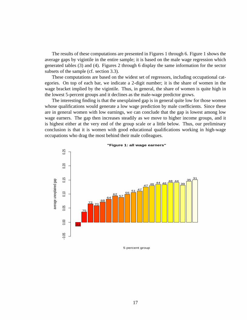
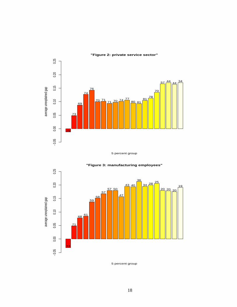
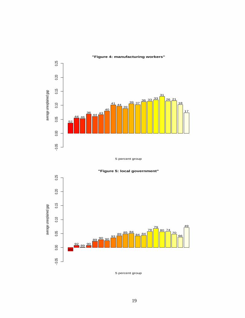
The results of these computations are presented in Figures 1 through 6. Figure 1 shows theaverage gaps by vigintile in the entire sample; it is based on the male wage regression whichgenerated tables (3) and (4). Figures 2 through 6 display the same information for the sectorsubsets of the sample (cf. section 3.3).

These computations are based on the widest set of regressors, including occupational cat-egories. On top of each bar, we indicate a 2-digit number; it is the share of women in thewage bracket implied by the vigintile. Thus, in general, the share of women is quite high inthe lowest 5-percent groups and it declines as the male-wage predictor grows.

The interesting finding is that the unexplained gap is in general quite low for those womenwhose qualifications would generate a low wage prediction by male coefficients. Since theseare in general women with low earnings, we can conclude that the gap is lowest among lowwage earners. The gap then increases steadily as we move to higher income groups, and itis highest either at the very end of the group scale or a little below. Thus, our preliminaryconclusion is that it is women with good educational qualifications working in high-wageoccupations who drag the most behind their male colleagues.

"Figure 1: all wage earners"

5 percent group

aver

age

unex

plaine

d ga

p

−0.0

50.

000.

050.

100.

150.

200.

25

82

75

7270

6864

6257

5551 47

47 46 44 4848 44

3935

31

17

"Figure 2: private service sector"

5 percent group

aver

age

unex

plaine

d ga

p

−0.0

50.

000.

050.

100.

150.

200.

25

79

73

69

74

76

70 7171 70 74 77

80 8181

78

70

57 4444

34

"Figure 3: manufacturing employees"

5 percent group

aver

age

unex

plaine

d ga

p

−0.0

50.

000.

050.

100.

150.

200.

25

73

71

6861

5958

5757 50

47

43 40

36

34 2825

20 20 20

19

18

"Figure 4: manufacturing workers"

5 percent group

aver

age

unex

plaine

d ga

p

−0.0

50.

000.

050.

100.

150.

200.

25

52

44 46

3644

4340

41 4439

39 3736 33 33

31

26 2118

17

"Figure 5: local government"

5 percent group

aver

age

unex

plaine

d ga

p

−0.0

50.

000.

050.

100.

150.

200.

25

89

9289

90

8990 90

9389

85 8484 84

7879

80 7470

66

49

19

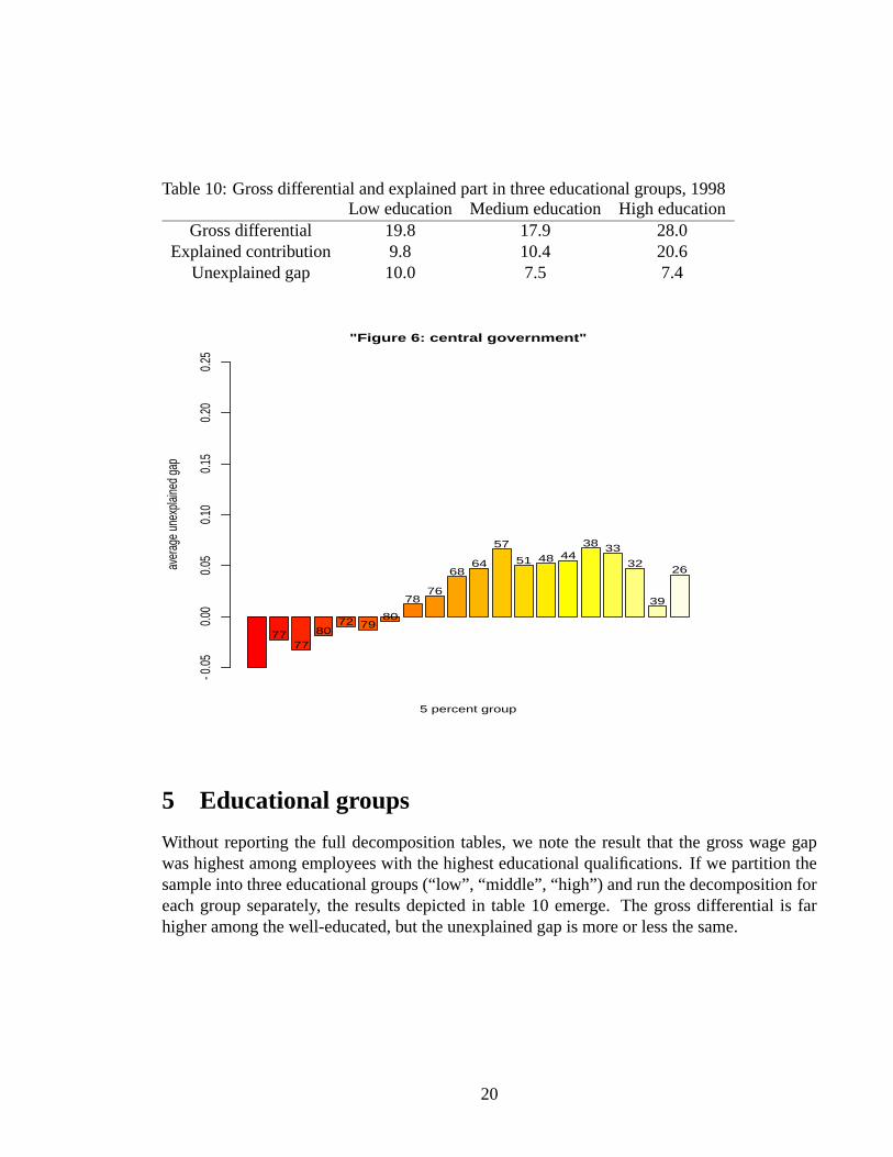
Table 10: Gross differential and explained part in three educational groups, 1998Low education Medium education High education

Gross differential 19.8 17.9 28.0Explained contribution 9.8 10.4 20.6

Unexplained gap 10.0 7.5 7.4

"Figure 6: central government"

5 percent group

aver

age

unex

plaine

d ga

p

−0.0

50.

000.

050.

100.

150.

200.

25

7777

8072 79

80

7876

6864

57

51 48 4438 33

32

39

26

5 Educational groups

Without reporting the full decomposition tables, we note the result that the gross wage gapwas highest among employees with the highest educational qualifications. If we partition thesample into three educational groups (“low”, “middle”, “high”) and run the decomposition foreach group separately, the results depicted in table 10 emerge. The gross differential is farhigher among the well-educated, but the unexplained gap is more or less the same.

20

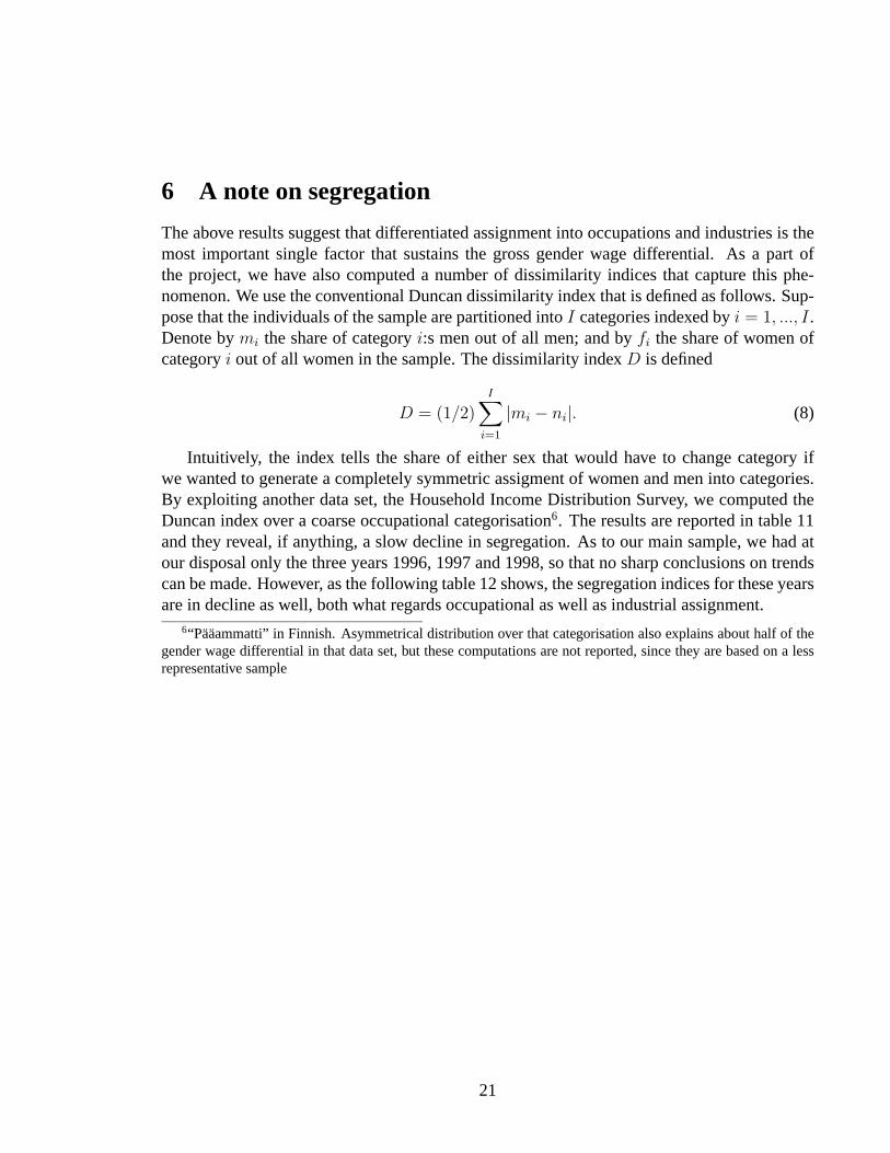
6 A note on segregation

The above results suggest that differentiated assignment into occupations and industries is themost important single factor that sustains the gross gender wage differential. As a part ofthe project, we have also computed a number of dissimilarity indices that capture this phe-nomenon. We use the conventional Duncan dissimilarity index that is defined as follows. Sup-pose that the individuals of the sample are partitioned intoI categories indexed byi = 1, ..., I.Denote bymi the share of categoryi:s men out of all men; and byfi the share of women ofcategoryi out of all women in the sample. The dissimilarity indexD is defined

D = (1/2)I∑i=1

|mi − ni|. (8)

Intuitively, the index tells the share of either sex that would have to change category ifwe wanted to generate a completely symmetric assigment of women and men into categories.By exploiting another data set, the Household Income Distribution Survey, we computed theDuncan index over a coarse occupational categorisation6. The results are reported in table 11and they reveal, if anything, a slow decline in segregation. As to our main sample, we had atour disposal only the three years 1996, 1997 and 1998, so that no sharp conclusions on trendscan be made. However, as the following table 12 shows, the segregation indices for these yearsare in decline as well, both what regards occupational as well as industrial assignment.

6“Pääammatti” in Finnish. Asymmetrical distribution over that categorisation also explains about half of thegender wage differential in that data set, but these computations are not reported, since they are based on a lessrepresentative sample

21

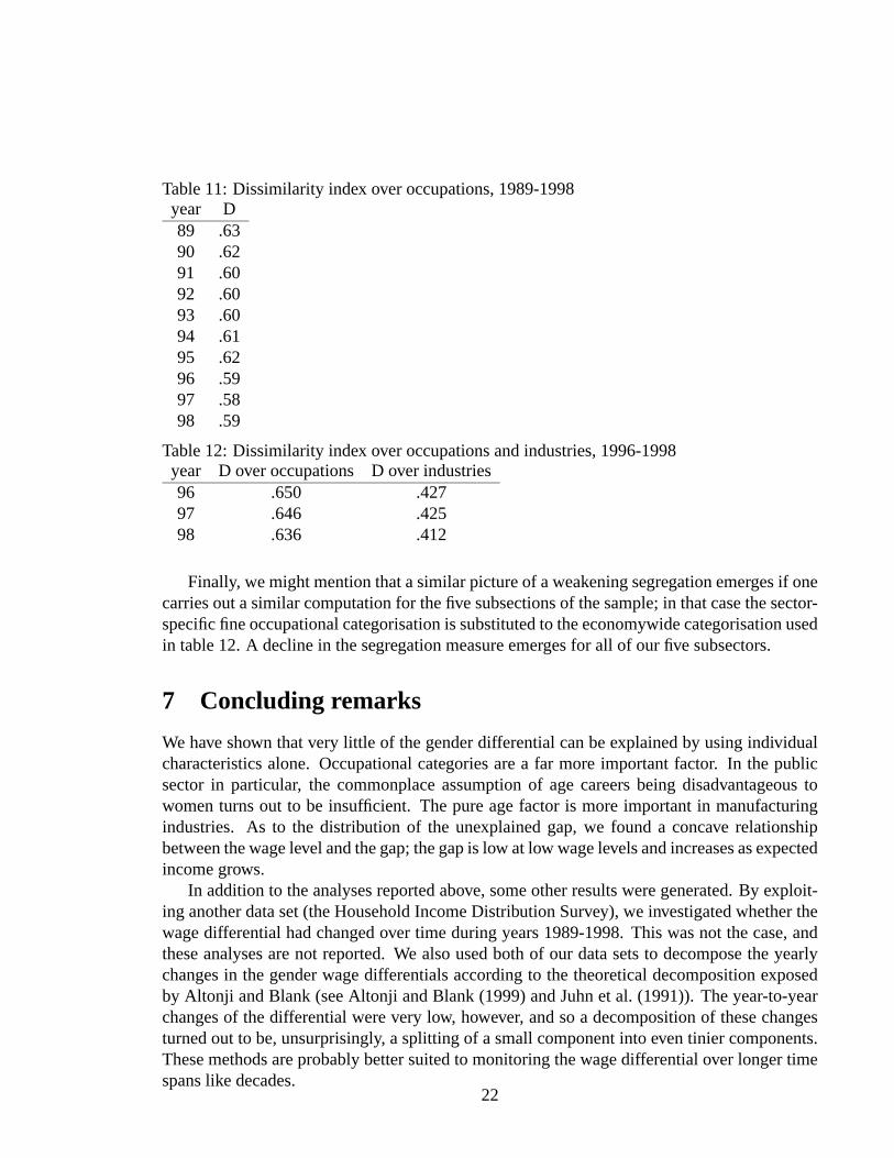
Table 11: Dissimilarity index over occupations, 1989-1998year D89 .6390 .6291 .6092 .6093 .6094 .6195 .6296 .5997 .5898 .59

Table 12: Dissimilarity index over occupations and industries, 1996-1998year D over occupations D over industries96 .650 .42797 .646 .42598 .636 .412

Finally, we might mention that a similar picture of a weakening segregation emerges if onecarries out a similar computation for the five subsections of the sample; in that case the sector-specific fine occupational categorisation is substituted to the economywide categorisation usedin table 12. A decline in the segregation measure emerges for all of our five subsectors.

7 Concluding remarks

We have shown that very little of the gender differential can be explained by using individualcharacteristics alone. Occupational categories are a far more important factor. In the publicsector in particular, the commonplace assumption of age careers being disadvantageous towomen turns out to be insufficient. The pure age factor is more important in manufacturingindustries. As to the distribution of the unexplained gap, we found a concave relationshipbetween the wage level and the gap; the gap is low at low wage levels and increases as expectedincome grows.

In addition to the analyses reported above, some other results were generated. By exploit-ing another data set (the Household Income Distribution Survey), we investigated whether thewage differential had changed over time during years 1989-1998. This was not the case, andthese analyses are not reported. We also used both of our data sets to decompose the yearlychanges in the gender wage differentials according to the theoretical decomposition exposedby Altonji and Blank (see Altonji and Blank (1999) and Juhn et al. (1991)). The year-to-yearchanges of the differential were very low, however, and so a decomposition of these changesturned out to be, unsurprisingly, a splitting of a small component into even tinier components.These methods are probably better suited to monitoring the wage differential over longer timespans like decades.

22

However, one positive development could be reported on the evolution of dissimilarityindices over time. Using both of our data sets, we computed the Duncan dissimilarity indexover occupational classification and industrial classification. In all of these indicators, a slowbut statistically significant trend towards less segeration emerges.

Hopefully, the methods and results of the project reported here can contribute to a moreregular and systematic monitoring of the gender wage differential in future. Similar methodscan also serve the purpose of comparative work and adoption of best practices within theEuropean Union7.

7Indeed, the Belgian presidency’s proposition on Indicators in Gender Pay Equality follows a rather similarline of thought.

23

References

Altonji, J. G. and Blank, R. M. (1999). Race and gender in the labor market. In Ashenfelter,O. and Card, D., editors,Handbook of Labor Economics. Elsevier Science.

Jenkins, S. (1994). Earnings discrimination measurement: a distributional approach.Journalof Econometrics, 61(1):81–102.

Juhn, C., Murphy, K., and Pierce, B. (1991). Accounting for the slowdown in black-whitewage convergence. In Kosters, M., editor,Workers and their wages. AEI Press, WashingtonDC, Washington DC.

Oaxaca, R. (1973). Male-female wage differentials in urban labor markets.InternationalEconomic Review, 14(3):693–709.

Oaxaca, R. and Ransom, M. (1994). On discrimination and the decomposition of wage differ-entials.Journal of Econometrics, 61:5–21.

Oaxaca, R. and Ransom, M. (1999). Identification in detailed wage decompositions.Reviewof Economics and Statistics, 81(1):154–157.

Vartiainen, J. (2001).Sukupuolten palkkaeron tilastointi ja analyysi. Number 2001:17 inTasa-arvojulkaisuja. Sosiaali- ja terveysministeriö.

24

Government & Nonprofit

Gender Wage Differentials in the Finnish Labour Market