222EDUCATIONPOLICY AND

INTERGENERATIONALINCOME MOBILITY: EVIDENCE FROM

THE FINNISH COMPREHENSIVE SCHOOL REFORM

Sari PekkalaTuomas Pekkarinen

Roope Uusitalo

PALKANSAAJIEN TUTKIMUSLAITOS • TYÖPAPEREITA LABOUR INSTITUTE FOR ECONOMIC RESEARCH • DISCUSSION PAPERS

This is an updated version of the paper previously published as IZA Discussion Paper 2204 in July 2006. The authors would like to thank David Autor, Nils Gottfries, Markus Jäntti, Mikael Lindahl and

the seminar participants in Mannheim, Stockholm, Turku, Helsinki and Uppsala for helpful comments. The authors are grateful to the Statistics Finland and especially Marianne Johnson and Christian

Starck for their help with the data.

Helsinki 2006

222

Education policy and intergenerational income mobility: Evidence from the Finnish comprehensive school reform

Tuomas Pekkarinen Roope Uusitalo Sari Pekkala

ISBN 952−209−029−8 ISSN 1795−1801

1

Abstract

This paper estimates the effect of a major education reform on the intergenerational income

mobility in Finland. The Finnish comprehensive school reform of 1972-1977 replaced the old

two-track school system with a uniform nine-year comprehensive school and significantly

reduced the degree of heterogeneity in the Finnish primary and secondary education. We

estimate the effect of this reform on the intergenerational income elasticity using a

representative sample of males born during 1960-1966. The identification strategy relies on a

difference-in-differences approach and exploits the fact that the reform was implemented

gradually across country during a six-year period. The results indicate that the reform

reduced the intergenerational income elasticity by about seven percentage points.

1 Introduction

One of the key questions in the study of economic inequality is the degree to which the

economic status is transferred within families. It is often argued that high cross-sectional

inequality is socially more sustainable if it is accompanied with high intergenerational

mobility. In a highly mobile society, each incoming cohort is faced with equal opportu-

nities to climb up the income distribution and neither wealth nor poverty is necessarily

inherited from the parents.

The most common approach to study intergenerational income mobility in economics

is to estimate correlations of lifetime earnings of fathers and their sons. More than two

decades of research has shown that there are large di¤erences in mobility across coun-

tries. Income mobility is low and intergenerational income correlation high (around 0.4)

in the United States and the United Kingdom. Mobility is much higher and intergener-

ational income correlation lower (around 0.2) in Canada, Finland, and Sweden.1 Recent

research also indicates that these correlations have been increasing in the United States

and the United Kingdom over the last two decades. In Finland, on the other hand, in-

tergenerational income correlation has followed a steady downward trend over last thirty

years.2

Apart from these facts, however, little is known about the mechanisms underlying

the intergenerational persistence in income or about the reasons behind the cross-country

di¤erences. Also, even though recent research has started to document changes in social

mobility, there is little hard evidence on the causes of the observed changes. Perhaps

most importantly, there is no evidence on the e¤ects of feasible policy instruments that

1See Solon (1992) and Zimmerman (1992) on US; Dearden, Machin, and Reed (1997) on UK; Corakand Heisz (1999) on Canada; Björklund and Jäntti (1997) on Sweden; and Österbacka (2001) on Finland.

2See Aaronson and Mazumder (2005) on the trends in the US; Blanden, Goodman, Gregg, and Machin(2004) on the trends in the UK, and Pekkala and Lucas (2006) on the trends in Finland. Interestingly,Pekkala and Lucas also demonstrate that the decrease in intergenerational correlation in Finland is mainlydue to a decrease in the returns to education and to the lessening impact of family income on educationalattainment.

2

could a¤ect income mobility. It would be interesting to know whether programs that aim

to alleviate the adverse e¤ects of poor family background actually succeed in equalizing

economic opportunities.

In this paper, we estimate the e¤ects of one such policy by examining the impacts

of the Finnish comprehensive school reform implemented between 1972 and 1977. The

Finnish school reform is a good example of the educational reforms that were implemented

in Europe after the second world war. Very similar reforms took place in Sweden in the

1950s and in Norway in the 1960s.3 These reforms were seen as an integral part in the

building of modern welfare state and one of the main motivations for their implementation

was precisely to enhance the equality of opportunity.

The Finnish reform replaced old two track school system with a nine year compre-

hensive school and imposed a uniform academic curriculum on the entire cohort until age

16. This kind of reform should have an impact on the intergenerational for a number

of reasons. First, the reform increased the length of compulsory schooling from eight to

nine years. If the return to increased years of schooling are positive and if those with

low income parents are more likely to quit school after compulsory schooling, the reform

will have the largest e¤ect on the students from low-income families. Second, the reform

signi�cantly reduced the heterogeneity in the quality of primary and secondary educa-

tion. Third, the reform postponed the age when the students are tracked to academic

and vocational schooling from eleven to sixteen. If family background has a larger im-

pact on early education choices postponing the tracking age lessens the e¤ect of family

background on educational attainment. Finally, keeping the entire cohort together in the

same schools increases the heterogeneity of the peer groups which may also reduce the

e¤ect of family background. Holmlund (2006), for example, shows that more diverse peer

3See Lechinsky and Mayer (1990) for an overview of the comprehensive school reforms in post-warEurope.

3

groups decreased the degree of assortative mating after a similar reform in Sweden and

that the reduction of assortative mating ampli�es the e¤ects of comprehensive school on

the intergenerational income correlation.

The e¤ects of this kind of reform are also interesting because educational policies

play a key role in the theoretical literature on intergenerational income mobility, start-

ing from the work by Becker and Tomes (1979, 1986) and developed by Solon (2004).

More recently, Restuccia and Urrutia (2004) have presented a model that distinguishes

between early and late education and argue that the intergenerational income persistence

is driven by parental investment in the primary and secondary education of their children.

This model is in line with the growing literature on the technology of the skill formation

surveyed by Carneiro and Heckman (2003) as well as Cunha, Heckman, Lochner, and

Masterov (2006). According to these authors, the production of human capital is charac-

terized by strong complementarity of skills that are acquired early and investment in later

education. Hence, policy interventions that target early education of individuals from a

disadvantaged background will increase the returns to both private and public investment

in post-secondary education, and are likely to lead to increased income mobility.

Finally, there is some evidence that suggests that the aspects of the educational sys-

tems such as tracking and the heterogeneity in the quality of early education a¤ect in-

tergenerational income mobility. Dustmann (2004) argues that high intergenerational

income correlation in Germany is at least partly due to the German educational system

where pupils are tracked to academic and vocational schools already at the age of 10. In

line with this argument, Meghir and Palme (2005) show that the comprehensive school

reform in Sweden had a particularly strong e¤ect on the education and income of high

ability pupils with less educated parents.

We estimate the e¤ect of the reform on the elasticity of son�s earnings in 2000 with

respect to father�s average earnings during 1970-1990 using a representative sample of

4

males born between 1960 and 1966. The identi�cation strategy relies on a di¤erences-

in-di¤erences approach and exploits the fact that the reform was implemented gradually

during a six-year period. The overall intergenerational income elasticity in this sample

is 0.28. The reform decreased the intergenerational income elasticity by approximately

seven percentage points from the pre-reform elasticity of 0.30 or by approximately 20

percent.

The paper is organized as follows. In the following section, we describe the Finnish

comprehensive school reform in detail and argue why it provides a good natural experi-

ment to study the e¤ects of educational policies on intergenerational income correlation.

Our identi�cation strategy is described in more detail in section 3. We then present the

sample from the Finnish Longitudinal Census Data Files that we use in our analysis and

in the �fth section we present the results. The sixth section concludes.

2 The Finnish comprehensive school reform 1972-1977

Finland followed the example of her Nordic neighbors and introduced a thorough com-

prehensive school reform in the 1970�s. Similar reforms had taken place earlier in Sweden

and Norway. These reforms are described in detail in Meghir and Palme (2004) and

Aalvik, Salvanes and Vaage (2003). The main motivation for the reform was to provide

equal educational opportunities to all students irrespective of place of residence or social

background. Rapid re-structuring of the Finnish economy probably also played a role.

The demand for low-skill labor in small farms and forestry had decreased rapidly. The

growing industrial sector increased the demand for skilled workers.

Prior to the comprehensive school reform, Finland had a two-track school system. In

this system, cohorts attended uniform education only for four years after which they were

divided into two tracks that di¤ered both in the content of education, as well as, in the

5

eligibility that they provided for further education.

The pre-reform system is described schematically in the left-hand panel of Figure 1.

All students entered primary school (kansakoulu) at age seven. After four years in the

primary school, at age 11, the students were faced with the choice of applying to general

secondary school (oppikoulu) or continuing in the primary school. Admissions to the

general secondary school were based on an entrance examination, a teacher assessment

and primary school grades. Those who were admitted continued their schooling in the

junior secondary schools for �ve years and often went on to the upper secondary school

for three additional years. At the end of the upper secondary school the students took

the matriculation examination that provided eligibility to university-level studies.

Those who were not admitted or who did not apply to the general secondary school

continued in primary school for two more years, and spent in total six years in the primary

school. By the beginning of 1970s most primary schools had continuation classes (civic

schools) that kept almost the whole age cohort at school up to the 8th (and in many

municipalities 9th) grade. This education did not provide eligibility for senior secondary

school or for university studies. After civic school most students continued into vocational

education or �nished their schooling.

In 1970, most secondary schools were private. About 55 percent of all general sec-

ondary school students attended these private schools. The private schools collected

student fees but received most of their funding as state aid and contributions from lo-

cal municipalities. The fraction of students in the state schools was about 30 percent.

The remaining 15 percent attended municipality-run secondary schools, mostly founded

during the 1960s.

The curriculum in general secondary schools was very di¤erent from the more prac-

tical civic schools. For example, foreign languages were compulsory only in the general

secondary school. These schools also taught more advanced mathematics and science

6

whereas the focus in civic schools was on practical skills required in low-skill occupations.

[FIGURE 1: SCHOOL SYSTEMS]

2.1 Content of the comprehensive school reform

The school system was reformed in the 1970s. The post-reform system is described

in the right-hand panel of �gure 1. Previous primary school, civic school and junior

secondary school were replaced by a nine-year comprehensive school. At the same time

upper secondary school was separated from the junior secondary school to form a distinct

institution. After the reform, all the pupils followed the same curriculum in the same

establishments (comprehensive schools) up to age 16. After this, the students chose

between applying to upper secondary school or to vocational schools. Admission to both

tracks was based solely on comprehensive school grades.

The reform also introduced a new curriculum and changed the structure of primary and

secondary education. The new curriculum increased the academic content of education

compared to the old primary school curriculum by increasing the share of mathematics and

sciences. In addition, one foreign language became compulsory for all students. Thus,

the new comprehensive school curriculum resembled the old general secondary school

curriculum and exposed the pupils who, in the absence of the reform, would have stayed

in the primary school to a signi�cantly more academic education.

Hence, the main changes that followed the reform were the postponement of tracking

from the age 11 to 16 and the increase in the academic content of the curriculum. In

addition to these fundamental changes, the reform also imposed a centralized control

on schools at the national level and almost abolished the extensive network of private

schools that had run general secondary school system by placing them under municipal

ownership.

7

2.2 The implementation of the comprehensive school reform

The implementation of the reform was preceded by a process of planning that lasted for

two decades. Government working groups had proposed creating comprehensive school

as early as in 1948. The �rst experimental comprehensive schools started their operation

in 1967. Finally, in 1968 the parliament approved School Systems Act (467/1968) accord-

ing to which the two track school system would be gradually replaced with a nine-year

comprehensive school. The adoption of the new school system was to take place between

1972 and 1977 and the order in which the municipalities adopted the reform was to be

determined by geography starting from the Northern Finland where access to education

was most limited. A regional implementation plan divided the country into six imple-

mentation regions and dictated when each region would adopt the comprehensive school

system. Regional school boards were created to oversee the transition process.

In each region, the �ve lowest primary school grades were to start in the comprehensive

school immediately in the fall term of the year stated in the regional implementation plan.

After this, each incoming cohort would start their schooling in the comprehensive school.

The pupils that were already above the �fth grade in the year that the region started the

reform would complete their schooling according to the pre-reform system. Thus, in each

region it took approximately four years to complete the reform so that all the pupils in

the grades 1-9 were in the comprehensive school.

Figure 2 illustrates how the reform spread through Finland during 1972-1977. The

�rst municipalities that adopted the reform in 1972 were predominantly situated in the

northernmost province of Lapland. In 1973 the reform was mostly adopted in the north-

eastern regions. From thereon, the reform spread so that it was adopted in 1974 in the

northwest, in 1975 in south-east, in 1976 in the south-west, and �nally, in 1977 in the

capital region of Helsinki.

8

[FIGURE 2: MAP]

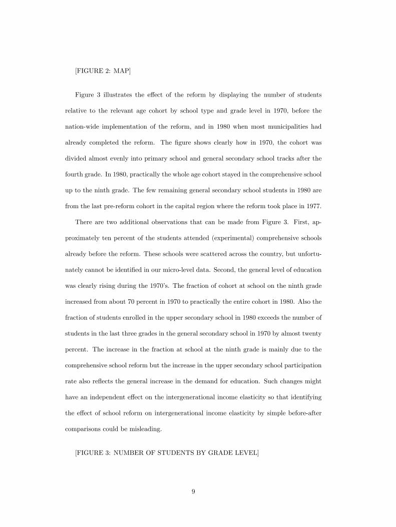
Figure 3 illustrates the e¤ect of the reform by displaying the number of students

relative to the relevant age cohort by school type and grade level in 1970, before the

nation-wide implementation of the reform, and in 1980 when most municipalities had

already completed the reform. The �gure shows clearly how in 1970, the cohort was

divided almost evenly into primary school and general secondary school tracks after the

fourth grade. In 1980, practically the whole age cohort stayed in the comprehensive school

up to the ninth grade. The few remaining general secondary school students in 1980 are

from the last pre-reform cohort in the capital region where the reform took place in 1977.

There are two additional observations that can be made from Figure 3. First, ap-

proximately ten percent of the students attended (experimental) comprehensive schools

already before the reform. These schools were scattered across the country, but unfortu-

nately cannot be identi�ed in our micro-level data. Second, the general level of education

was clearly rising during the 1970�s. The fraction of cohort at school on the ninth grade

increased from about 70 percent in 1970 to practically the entire cohort in 1980. Also the

fraction of students enrolled in the upper secondary school in 1980 exceeds the number of

students in the last three grades in the general secondary school in 1970 by almost twenty

percent. The increase in the fraction at school at the ninth grade is mainly due to the

comprehensive school reform but the increase in the upper secondary school participation

rate also re�ects the general increase in the demand for education. Such changes might

have an independent e¤ect on the intergenerational income elasticity so that identifying

the e¤ect of school reform on intergenerational income elasticity by simple before-after

comparisons could be misleading.

[FIGURE 3: NUMBER OF STUDENTS BY GRADE LEVEL]

9

2.3 The comprehensive school reform as a quasi-experiment

The Finnish comprehensive school reform is in many ways an ideal experiment for evaluat-

ing the e¤ects of early versus late tracking on the intergenerational income elasticity. The

regional implementation plan dictated when each municipality moved into comprehen-

sive school system. Using a �xed-e¤ects approach we can control for other simultaneous

time trends and regional di¤erences and purge the estimate of school system from these

confounding factors.

Yet, as in any real world reform there are some caveats to the approach. First of

all, as is clear from �gure 2, the geographical implementation plan assigned some mu-

nicipalities to early implementation groups even though most surrounding municipalities

implemented the reform much later. The choice of municipalities to these early imple-

mentation groups was probably not entirely random. The comprehensive school reform

also faced intensive resistance. Most common arguments against the reform were that

abolishing tracking would reduce the quality of education. As a compromise, ability

tracking was partially retained within the comprehensive school. Even after the reform

the students were divided into ability groups in foreign language and math classes, but

studied all other subjects in their regular (not tracked) classes. This ability grouping was

eventually abolished in 1985.

The socialization of private schools under municipal ownership was also opposed es-

pecially in Helsinki where some of these schools had a distinguished reputation. After an

intensive debate, it was agreed that several private schools would be allowed to survive

as private alternatives to the comprehensive schools in the Helsinki region even after the

reform. Many of these still exist as private senior secondary schools. Another important

point to note is that in several municipalities municipality-run experimental comprehen-

sive schools already took in almost the whole age cohort a few years before the reform.

10

In these municipalities the founding of these schools probably had a larger e¤ect than the

subsequent transformation to a comprehensive school.

What is common to these factors is that they imply that the implementation of the

reform in practice did not necessarily follow the implementation plan. One would expect

these factors to attenuate the e¤ects of the reform on intergenerational income mobility,

but the size of the bias is di¢ cult to assess. As a rough check on how contaminated the

implementation of the reform actually was, we examined data from the Finnish Adult

Education Surveys in 1990, 1995 and 2000. We linked the municipality where the re-

spondents lived in 1975 to the survey data and classi�ed these municipalities into regions

according to the year when the comprehensive school reform took place in these munic-

ipalities. Then we calculated the fraction of respondents whose highest education was

primary school by regions and birth cohorts. The main lesson from these calculations

was that the reform clearly had an impact. Very few respondents report primary school

as highest education after the reform and these can easily be explained by regional mo-

bility. Also timing of the reform matches the timing of the reduction of the share with

primary school as the highest education, though in most regions the fraction with only

compulsory school decreases already one to two years before the reform.4

3 Estimation methods

Our goal is to estimate the changes in the intergenerational income elasticity due to

the comprehensive school reform. The identi�cation strategy relies on a di¤erence-in-

di¤erences approach and exploits the fact that the reform was implemented gradually

during a six-year period.

We start with the standard speci�cation relating the lifetime earnings of the son (ys)

4Details on these calculations can be found from an appendix available upon request.

11

to the lifetime earnings of his father (yf ).

log(ys) = a+ bjt log(yf ) + e (1)

The regression coe¢ cient b provides an estimate of the intergenerational income elas-

ticity. In order to examine how the reform a¤ected this elasticity, we allow this regression

coe¢ cient to vary across cohorts, regions, and the reform status:

bjt = b0 + �Rjt +Dj +Dt + ujt (2)

where j indexes region of residence, and t the birth cohort. Rjt is a dummy variable

equal to 1 if the reform had taken place in the municipality by the time when the son was

in the relevant age, Dj is the full set of region �xed e¤ects, and Dt a full set of cohort

dummies. Including a full set of cohort and region �xed-e¤ects allows the intergenera-

tional income elasticity to change over time and to vary across regions. Including cohort

dummies also accounts for the fact that later cohorts are observed at a younger age and

their earnings may be worse proxies of lifetime income. The only identifying assumption

we impose is that the changes in intergenerational income elasticity are not systematically

di¤erent in the di¤erent regions. The parameter � identi�es the e¤ect of the reform on

the intergenerational income elasticity.

Inserting expression (2) back into the regression equation (1) and adding the main

e¤ects of the region and time, as well as, the main e¤ect of the reform produces

log(ys;jt) = a+ b0 log yf + �(log yf �Rjt) + (log yf �Dj) + (log yf �Dt) + log yf � ujt

+�Dt +�Dj + �Rjt + eijt (3)

Estimating the e¤ect of the comprehensive school reform on intergenerational income

12

elasticity, therefore, reduces to a model where the son�s log lifetime earnings are regressed

on the father�s log lifetime earnings interacted with the reform dummy, and a full set of

interactions between region and the cohort dummies and the father�s lifetime earnings.5

The e¤ect of the reform is identi�ed from second level interactions i.e. from the changes

in the e¤ect of father�s income occurring at the time of the reform.

4 Data

The data that we use in this paper come from the Finnish Longitudinal Census Data Files

(FLCD) by Statistics Finland.6 Information is based on population census conducted

every �fth year between 1970 and 2000. Currently the Finnish census is entirely register-

based and uses personal identity codes to merge information from various administrative

registers. Up to 1980 census contained also a questionnaire mailed to every household,

but even in 1970s variables such as annual earnings were based on tax registers.

Data contain information on all the 6.3 million individuals who had legal residence in

Finland in at least one census year. As these data are based on administrative registers,

the only reasons for the individual not to appear in the data are death and emigration.

Hence, these data do not have the attrition problems that are common in the intergen-

erational studies. Census �les also allow matching individuals across census years and

matching family members to each other.

Our data is a 10 percent random sample from the cohorts born between 1960 and

1966. We chose to restrict the analysis to these cohorts to have two cohorts, 1960 and

5It should be noted that equation (3) is actually a random coe¢ cient model with a heteroskedasticerror term, which needs to be accounted when calculating standard errors for the estimates.

6Data used in the analysis contain con�dental information based on tax registers. All datasetsused in the paper and their English language descriptions are available from the authors forreplication purposes but data access requires a prior approval by Statistics Finland. Details ondata access policy and application procedure can be found from the Statistics Finland website athttp://www.stat.�/meta/tietosuoja/kayttolupa_en.html. The authors are willing to assist in any way ingaining access to the data.

13

1966, with individuals only in the pre- and in the post-reform school systems and �ve

cohorts, 1961-1965, with individuals in both systems. We can track these individuals in

all census years from 1970 to 2000. To be comparable with most of the earlier literature

we focus on fathers and their sons. With our data similar analysis could also be performed

for mothers and daughters.

We measured sons�earnings as log taxable earnings in 2000. The measure includes

both employment and self-employment earnings, as well as, all taxable bene�ts (e.g.

unemployment bene�ts). In 2000, the youngest cohort in our sample was 34 and the

oldest 40 years old As noted above, we account for age of measurement by allowing the

e¤ect of father�s earnings to depend on son�s age. In some robustness checks we also use

earnings from 1995 and take the average from these two years. The main problem in

using earlier years is that Finnish students graduate relatively late. In 1995 the youngest

cohorts are only 29 years of age and many have just �nished school or are still studying

at a university. We also experimented with trimming the data in various ways to reduce

the e¤ects of extreme observations on sons�earnings but this had only a minor e¤ect on

our estimates.

To calculate fathers lifetime earnings we took the average log taxable earnings from

1970, 1975, 1980, 1985, and 1990 all de�ated to the 2000 prices. We calculated the aver-

age log earnings including all years with positive earnings. Using �ve years of data over

a time span of twenty years reduces the bias caused by measurement error in fathers�

earnings. To further reduce the e¤ect of measurement errors, we top-coded the highest 1

percent of fathers�s earnings by replacing them with 99th percentile of the fathers�earn-

ings distribution and similarly bottom-coded the lowest one percent of fathers�earnings

replacing them with the 1st percentile. We have no information on fathers�age so we

cannot make further adjustments that would account for observing fathers at di¤erent

ages.

14

The original data does contain information on the municipality of residence but this

information is not released to users so that individuals could not be identi�ed. From

our request the Statistics Finland classi�ed the municipalities of residence in 1970, 1975,

and 1980 to six groups according to the year when the comprehensive school reform was

implemented in each municipality. We used this information together with information

on the birth dates to determine whether individual was a¤ected by the comprehensive

school reform. We classi�ed all individuals who were on the �fth grade or below when

the municipality adopted the reform to the treatment (comprehensive school) group.

As some of the e¤ect of the reform may be due to the e¤ect on schooling, a good

measure of years of education would be useful. Data contains information on the highest

degree completed that can be coded to years of education in a relatively straightforward

way. Unfortunately, only information on post-compulsory education is in the data. Our

education measure does not distinguish between primary and comprehensive schooling

nor between completing 7, 8 or 9 years of primary schooling and hence does not capture

the most relevant changes in the length of education after the reform.

The original 10% sample of the males born during 1960-1966 contains information on

27 109 individuals. Altogether, 1 909 of these individuals either died or moved out of

the country before year 2000. For 2 494 individuals the treatment status could not be

identi�ed because they moved between regions during their school years and 1 622 had no

father present. Finally, in most of our speci�cations we also drop the 260 individuals who

had no positive earnings in 2000. Our �nal analysis sample thus contains information on

20 824 individuals. Out of these, 9 695 (47 %) fall into the treatment group.

In Table 1, we report some summary statistics on the age and annual earnings of our

sample of individuals and their fathers. Sons�mean earnings are considerably higher than

fathers�mean earnings re�ecting the increase in real wages across the generations. Also

the standard deviation for sons�earnings is higher, mainly because fathers�earnings are

15

averaged across �ve years but sons�earnings measured based on a single year.

[TABLE 1: DESCRIPTIVE STATISTICS]

Table 2 further describes how the sample is divided into di¤erent cohorts and across

the reform regions. There are no large di¤erences in the cohort size in these age groups.

The most intense reform years were 1974, -75 and -76. The table also shows how the

treatment status depends on birth year and timing of the reform in the municipality of

residence. The 1960 cohort was not a¤ected by the reform in any region. Members of

the next cohort (born 1961) were a¤ected if they lived in a municipality that adopted the

reform in 1972 when they entered the �fth grade. The shaded area in the table indicates

the a¤ected groups in the younger cohorts. The table already indicates that there are a

number of potential di¤erence-in-di¤erences estimates that can be calculated to evaluate

the e¤ect of the reform.

[TABLE 2: TIMING OF REFORM BY COHORT]

5 Results

In table 3 we �rst report our estimates of the intergenerational elasticity of earnings sep-

arately by reform regions and birth cohorts. The �rst column of the upper panel displays

estimates by birth cohort. There is some indication of downward trend. The elasticity

falls from 0:30 for the 1960 birth cohort to 0:26 for the 1966 cohort. In addition to the

e¤ect of school reform, this drop may re�ect other di¤erences between cohorts, or the fact

that the earlier cohorts are older when we observe their earnings and intergenerational

earnings elasticity tends to increase with the age when sons�earnings are measured. In

the second and third columns we calculate these within cohort elasticities separately in

the regions where the reform had not taken place by the time when the cohort turned

16

eleven and in regions where the system was already reformed. The rightmost column

reports the within-cohort di¤erence between these regions. In all the birth cohorts, apart

from cohort born in 1961 and 1964, the estimated intergenerational earnings elasticity is

lower in the regions where reform had already taken place. These di¤erences, however,

are hardly ever signi�cant.

The bottom panel of table 3 repeats these calculations now examining changes over

time within regions. Looking down in the �rst column one can note that there are

substantial di¤erences across regions. In the second and third column the elasticities are

calculated separately for the pre- and post-reform cohorts. In all regions except the 1977

reform region, elasticity is lower among post-reform cohorts.

[TABLE 3: RESULTS BY REGION AND COHORT]

Table 4 presents the main regression results. In column 1, we report the results of

regressing the son�s log earnings in 2000 on the father�s average log earnings during 1970-

1990 without any control variables. The resulting coe¢ cient is 0.277 which is somewhat

higher than the earlier Finnish estimates. This is probably due to the fact that we measure

sons�earnings at a later age and use �ve-year averages of fathers�earnings. Jäntti and

Österbacka (1996) obtain an estimate of 0:22 using data for cohorts born between 1950 and

1960 with earnings measured in 1990. Österbacka (2001) obtains a much lower elasticity

estimate of 0.13 using data for the same cohorts. Both of these papers use only two-year

averages of fathers�earnings. Österbacka (2001) also includes sons�earnings from 1985

when the youngest sons are only 25 years old and many are still in school. Also Lucas

and Pekkala (2005) report a lower estimate of 0.19 for cohorts born between 1960 and

1964 with earnings measured at age 30.

In column 2, we add the reform dummy and the interaction between the reform dummy

and father�s earnings. The interaction term is �0:063 indicating that the intergenerational

17

earnings elasticity is lower after the reform. However, it would be premature to interpret

this di¤erence as the e¤ect of the reform. As is clear from table 3, there are systematic

di¤erences in the intergenerational income elasticity across both regions and cohorts and

the result in column 2 may simply re�ect the general downward trend in intergenerational

earnings elasticity or di¤erences in the e¤ect of fathers earnings between the regions that

adopted the reform early and those where the reform occurred later.

In column 3 we account for both of these factors by adding a full set of cohort and

region dummies and interacting these dummies with father�s earnings as described in

section 3. We normalize fathers� earnings, as well as, cohort and region dummies by

subtracting the sample mean. This has no e¤ect on our estimate on the e¤ect of the re-

form on intergenerational income elasticity (which is an interaction of cohort, region and

fathers�earnings) but makes the other coe¢ cients easier to interpret. For example, the

main e¤ect of fathers�earnings now refers to the average e¤ect in the sample before the

reform and not to the e¤ect in some speci�c region or in a speci�c cohort. The main e¤ect

of father�s earnings on son�s earnings in Column 3 is 0.298 which is close to our baseline

estimate in Column 1 and almost identical to the estimated pre-reform elasticity reported

in Column 2. The e¤ect of the reform on the intergenerational earnings elasticity i.e. the

coe¢ cient of the interaction between father�s earnings and the comprehensive school re-

form is �0:069, indicating that the comprehensive school reform reduced intergenerational

earnings elasticity by almost seven percentage points. This implies approximately 20%

decrease in the elasticity from the pre-reform average of 0:30. The estimate is statistically

signi�cant with a t-value of 3.11.

Interacting father�s earnings with the cohort and region dummies in Column 3 accounts

for any general trends and regional di¤erences in intergenerational income elasticity. It is

still possible that the changes in the intergenerational elasticity di¤er across regions for

reasons that are unrelated to the comprehensive school reform. In column 4 we account

18

for this by adding region-spreci�c linear trends in intergenerational income elasticity. For

completeness, we also include all interactions between the cohort and region dummies

to allow for any di¤erences in the growth rates of regional income. After adding these

interactions, the main e¤ect of the reform on the son�s earnings is no longer identi�ed.

However, the e¤ect of the reform on intergenerational income elasticity is still identi�ed.

The estimate is now -0.066 very close to that in the previous column and indicating that

at least the simplest regional trends cannot explain our �ndings.

[TABLE 4: REGRESSION RESULTS]

We implemented a number of robustness checks to the results reported in table 4.

These are reported in table 5. First, in column 1 we removed from the data all municipal-

ities that implemented the reform before the other municipalities in the same province.

In column 7 we removed observations from Helsinki region where the reform faced most

intense resistance. These attempts to control for potential endogeneity in the timing of

the reform had no major e¤ects on the results. The estimates are slightly higher than the

baseline estimates in Table 4, but not signi�cantly di¤erent.

In column 3 we replaced sons earnings in 2000 with average log earnings from 1995

and 2000. This yields somewhat lower estimate (-0.047). Also the main e¤ect of fathers�

earnings decreases and is now close to earlier Finnish estimates. These results suggest

that measuring sons�earnings at a younger age decreases the e¤ects of family background

perhaps because those with better educated parents tend to stay in school longer and

their earnings at younger age do not yet measure lifetime earnings very precisely. Finally,

in columns 4, 5, and 6 we remove top-coding, bottom-coding and both of these from

fathers�earnings. This has virtually no e¤ect on the results.

[TABLE 5: ROBUSTNESS]

19

In table 6, we estimate the e¤ects of the reform using all available pairwise comparisons

between cohorts and regions. For example, the �rst entry in the top panel uses data only

from cohorts born in 1960 and 1961 and reports the di¤erence-in-di¤erences estimate

based on the fact that only those born in 1961 who lived in the nothernmost part of the

country were exposed to the reform. The next estimate compares cohorts born in 1960 to

those born in 1962 and so on. Altogether there are 21 possible pairwise comparisons, 14

of which produce a negative point estimate. Also the distribution of the estimates does

not indicate that the overall estimates would be driven by some particular cohorts but

rather points to there being a general tendency of decreasing e¤ect of family background

after the reform. The lower panel repeats the same exercise using �fteen possible pairwise

comparisons between regions. Twelve of these point estimates turn out to be negative.

Again there is no indication of the e¤ect being due to particular regions.

[TABLE 6: PAIRWISE ESTIMATES]

In table 7 we examine the e¤ects of the reform by estimating the reform e¤ect sepa-

rately in quintiles de�ned according to the fathers�earnings. Each column presents the

results from a separate regression where sons�earnings are explained by the comprehen-

sive school reform, and dummy variables for the cohort and the region (Coe¢ cients of

the dummy variables are not reported in the table). No cross-equation restriction on the

size of the cohort or region e¤ects are imposed, so the estimates for the reform e¤ects

are essentially nonlinear version of those reported in table 4. The pattern of the results

is striking. The e¤ect of the reform decreases monotonously from a positive e¤ect of

0.036 in the lowest quintile to a negative e¤ect of -0.080 for the highest quintile. We also

repeated these calculations splitting the data according to father�s education with very

similar results. The negative point estimates in the highest quintiles also suggest that the

comprehensive school reform may have had negative e¤ects on some sub-groups. This

20

could be due to a decrease in quality of education in the comprehensive school compared

to the general secondary school before the reform, perhaps due to a more heterogenous

and, on average, poorer family background. However we would hesitate to make strong

conclusions given large standard errors on these estimates.

[TABLE 7 EFFECTS BY QUINTILE]

6 Conclusions

Even though the knowledge about intergenerational earnings correlations and their dif-

ferences across countries has quickly accumulated over the last ten years, understanding

about the mechanisms underlying these correlations is still incomplete. Many authors

have emphasized the potential role of educational institutions in shaping the intergenera-

tional earnings mobility. Especially the role of heterogeneity in the quality early education

has received attention. Yet, there is little direct evidence on the e¤ect of educational in-

stitutions on intergenerational earnings mobility.

In this paper we estimate the e¤ect of a major educational reform on the intergener-

ational earnings elasticity. The Finnish comprehensive school reform completely trans-

formed the structure and the content of the secondary education in Finland. As a result

of this reform, tracking to academic and vocational secondary education was postponed

from the age 11 to 16 and a uniform academic curriculum was imposed on entire cohorts

up to the ninth grade. The reform was adopted gradually by municipalities which allows

us to treat this reform as a quasi-experiment.

We �nd that the comprehensive school reform reduced the e¤ect of fathers�earnings on

the and sons�earnings by seven percentage points. This amounts to a 20 percent drop in

the intergenerational earnings correlation. These results suggest that policies that expand

21

the access to academic secondary education may signi�cantly enhance intergenerational

earnings mobility.

References

[1]Aakvik, Arild, Salvanes, Kjell G., and Kjell Vaage. 2003. �Measuring heterogeneity in

the returns to schooling in Norway using educational reforms�, Centre for Economic

Policy Research, Discussion paper No. 4088.

[2]Aaronson, Daniel and Bhashkar Mazumder. 2005. �Intergenerational economic mobil-

ity in the U.S. 1940 to 2000�, Federal Reserve Bank of Chicago, WP 2005-12.

[3]Becker, Gary S. and Nigel Tomes. 1979. �An equilibrium theory of the distribution

of income and intergenerational mobility�, Journal of Political Economy, 87:6, 1153-

1189.

[4]Becker, Gary S. and Nigel Tomes. 1986. �Human capital and the rise and fall of

families�, Journal of Labor Economics, July, Part 2, 4:3, S1-S39.

[5]Björklund, Anders and Markus Jäntti. 1997. �Intergenerational income mobility in

Sweden compared to the United States�, American Economic Review, 87:5, 110-118.

[6]Blanden, Jo, Alissa Goodman, Paul Gregg, and Stepgen Machin. 2004. �Changes

in intergenerational mobility in Britain�, in M. Corak (ed): Generational Income

Mobility in North America and Europe, Cambridge University Press.

[7]Carneiro, Pedro and James J. Heckman. 2003. �Human capital policy�, in James J.

Heckman and Alan B. Krueger (eds): Inequality in America: What Role for Human

Capital Policies?, MIT Press.

[8]Corak, Miles and Andrew Heisz. 1999. �The intergenerational earnings and income

22

mobility of Canadian men: Evidence from longitudinal income tax data�, Journal of

Human Resources, 34:3, 504-33.

[9]Cunha, Flavio., James J. Heckman, Lance Lochner, and David V. Masterov. 2005.

�Interpreting the evidence on life cycle skill formation�, IZA Discussion Paper No.

1675.

[10]Dearden, Lorraine, Stephen Machin, and Howard Reed. 1997. �Intergenerational mo-

bility in Britain�, Economic Journal, 107:440, 47-66.

[11]Dustmann, Christian. 2004. �Parental background, secondary school track choice, and

wages�, Oxford Economic Papers, 56, 209-230.

[12]Jäntti, Markus and Eva Österbacka. 1996. �How much of the variance in income can

be attributed to family background? Evidence from Finland�, unpublished.

[13]Leschinsky, Achim and Karin U. Mayer (eds). 1990. The Comprehensive School Ex-

periment Revisited: Evidence from Western Europe, Frankfurt am Main, Verlag Peter

Lang.

[14]Meghir, Costas and Mårten Palme. 2005. �Educational reform, ability, and parental

background�, American Economic Review, 95 (1), 414-424.

[15]Österbacka, Eva. 2001. �Family background and economic status in Finland�, Scan-

dinavian Journal of Economics, 103, 467-484.

[16]Pekkala, Sari and Robert E. B. Lucas. 2006. �On the importance of �nnishing school:

Half a century of inter-generational economic mobility in Finland�, Industrial Rela-

tions, forthcoming.

[17]Restuccia, Diego and Carlos Urrutia. 2004. �Intergenerational persistence of earnings:

23

The role of early and college education�, American Economic Review, 94 (4), 1354-

1378.

[18]Solon, Gary. 1992. �Intergenerational income mobility in the United States�, American

Economic Review, 82:3, 393-408.

[19]Solon, Gary. 2002: Cross-country di¤erences in intergenerational earnings mobility�,

Journal of Economic Perspectives, 16(3), 59-66.

[20]Solon, Gary. 2005. �A model of intergenerational mobility variation over time and

place�, in Corak, Miles . Generational Income Mobility in North America and Europe,

Cambridge University Press.

[21]Zimmerman, David J. 1992. �Regression towards mediocrity in economic structure�,

American Economic Review, 82:3, 409-429.

24

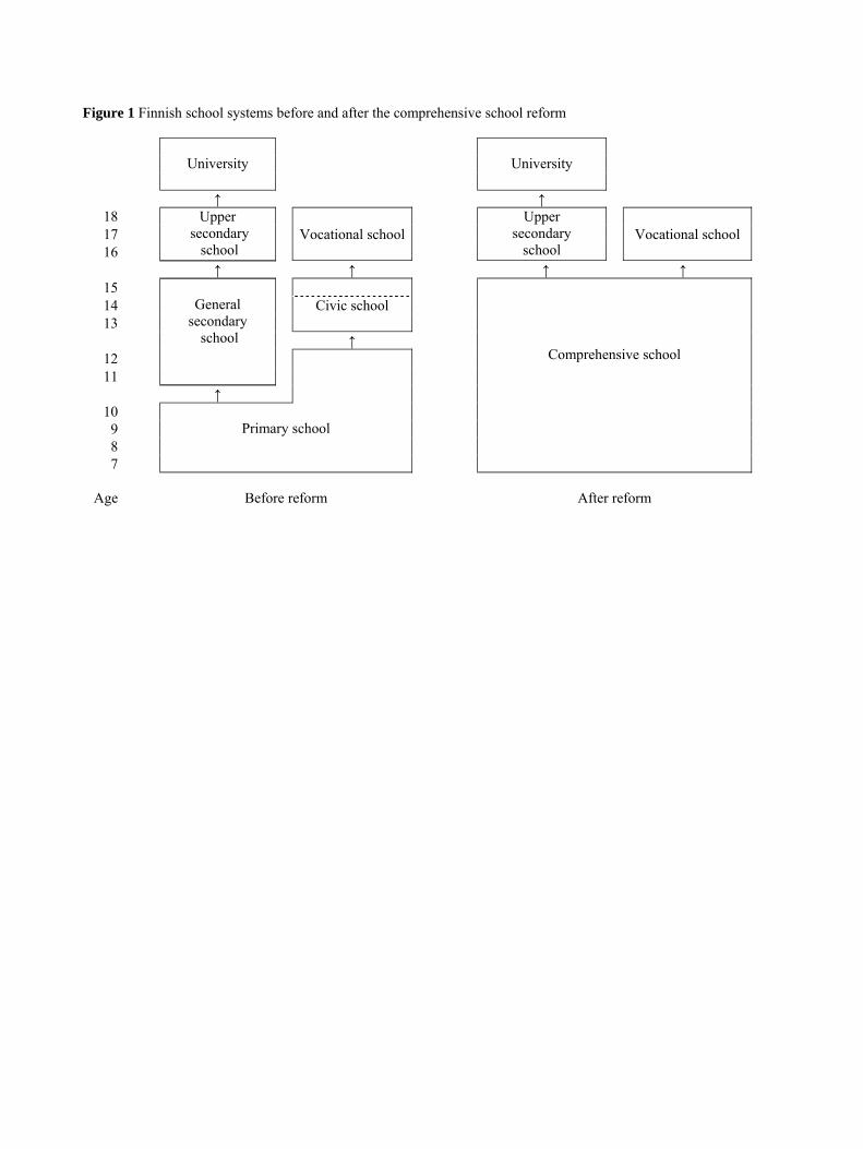
Figure 1 Finnish school systems before and after the comprehensive school reform

University

University

↑ ↑

18 17 16

Upper secondary

school Vocational school

Upper secondary

school Vocational school

↑ ↑ ↑ ↑ 15 14 13

Civic school

↑ 12 11

General

secondary school

↑

10 9 8 7

Primary school

Comprehensive school

Age

Before reform

After reform

Figure 2 The implementation of the comprehensive school reform across regions 1972-1977

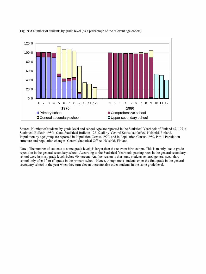
Figure 3 Number of students by grade level (as a percentage of the relevant age cohort)

0 %

20 %

40 %

60 %

80 %

100 %

120 %

1 2 3 4 5 6 7 8 9 10 11 12 1 2 3 4 5 6 7 8 9 10 11 121970 1980

Primary school Comprehensive schoolGeneral secondary school Upper secondary school

Source: Number of students by grade level and school type are reported in the Statistical Yearbook of Finland 67, 1971; Statistical Bulletin 1980:16 and Statistical Bulletin 1981:2 all by Central Statistical Office, Helsinki, Finland. Population by age group are reported in Population Census 1970, and in Population Census 1980, Part 1 Population structure and population changes, Central Statistical Office, Helsinki, Finland. Note: The number of students at some grade levels is larger than the relevant birth cohort. This is mainly due to grade repetition in the general secondary school. According to the Statistical Yearbook, passing rates in the general secondary school were in most grade levels below 90 percent. Another reason is that some students entered general secondary school only after 5th or 6th grade in the primary school. Hence, though most students enter the first grade in the general secondary school in the year when they turn eleven there are also older students in the same grade level.

Table 1 Summary statistics Variable Mean Std. Dev. Min Max Son’s age in 2000 37.03 1.98 34 40 Son’s earnings in 2000 29 778 110 544 100 14 916 700 Father’s average earnings during 1970-1990 18 687 11 832 800 69 041 Note: Summary statistics for 20 786 individuals in our sample and their fathers. Earnings refer to all taxable income in 2000 prices converted to euros.

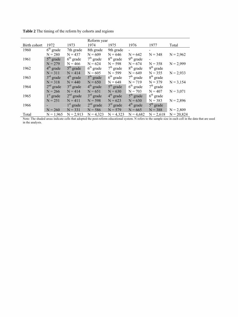
Table 2 The timing of the reform by cohorts and regions Reform year Birth cohort 1972 1973 1974 1975 1976 1977 Total 1960 6th grade 7th grade 8th grade 9th grade - - N = 280 N = 437 N = 609 N = 646 N = 642 N = 348 N = 2,962 1961 5th grade 6th grade 7th grade 8th grade 9th grade - N = 279 N = 466 N = 624 N = 598 N = 674 N = 358 N = 2,999 1962 4th grade 5th grade 6th grade 7th grade 8th grade 9th grade N = 311 N = 414 N = 605 N = 599 N = 649 N = 355 N = 2,933 1963 3rd grade 4th grade 5th grade 6th grade 7th grade 8th grade N = 318 N = 440 N = 650 N = 648 N = 719 N = 379 N = 3,154 1964 2nd grade 3rd grade 4th grade 5th grade 6th grade 7th grade N = 266 N = 414 N = 651 N = 630 N = 703 N = 407 N = 3,071 1965 1st grade 2nd grade 3rd grade 4th grade 5th grade 6th grade N = 251 N = 411 N = 598 N = 623 N = 630 N = 383 N = 2,896 1966 - 1st grade 2nd grade 3rd grade 4th grade 5th grade N = 260 N = 331 N = 586 N = 579 N = 665 N = 388 N = 2,809 Total N = 1,965 N = 2,913 N = 4,323 N = 4,323 N = 4,682 N = 2,618 N = 20,824 Note: The shaded areas indicate cells that adopted the post-reform educational system. N refers to the sample size in each cell in the data that are used in the analysis.

Table 3 Intergenerational income correlations across birth cohorts and reform regions a) Birth cohorts Birth cohort Average Pre-reform Post-reform Difference 1960 0.303 0.303 (0.021) (0.021) 1961 0.301 0.296 0.359 0.063 (0.021) (0.022) (0.064) (0.069) 1962 0.294 0.295 0.271 -0.024 (0.021) (0.025) (0.041) (0.048) 1963 0.244 0.313 0.141 -0.172 (0.022) (0.030) (0.034) (0.045) 1964 0.267 0.240 0.261 0.021 (0.022) (0.039) (0.028) (0.049) 1965 0.276 0.393 0.245 -0.147 (0.023) (0.070) (0.025) (0.072) 1966 0.262 0.262 (0.023) (0.023) b) Reform regions Region Average Pre-reform Post-reform Difference 1972 0.285 0.385 0.265 -0.119 (0.026) (0.068) (0.028) (0.071) 1973 0.234 0.293 0.211 -0.082 (0.021) (0.036) (0.027) (0.045) 1974 0.256 0.289 0.230 -0.058 (0.018) (0.027) (0.025) (0.037) 1975 0.257 0.273 0.242 -0.031 (0.019) (0.025) (0.031) (0.039) 1976 0.258 0.273 0.214 -0.060 (0.019) (0.021) (0.038) (0.044) 1977 0.322 0.314 0.391 0.077 (0.028) (0.030) (0.085) (0.086) Note: Numbers in the cells are coefficients of the father’s earnings in the regressions where son’s earnings are regressed on father’s earnings alone. Standard errors are reported in parentheses.

Table 4 Regression results (1) (2) (3) (4) Father's earnings 0.277 0.297 0.298 0.296 (0.014) (0.011) (0.010) (0.014) Reform -0.063 -0.019 … (0.012) (0.021) Father's earnings x Reform -0.055 -0.069 -0.066 (0.009) (0.022) (0.031)

Cohort dummies √ √

Father’s earnings * Cohort dummies √ √

Region dummies √ √

Father’s earnings * Region dummies √ √

Cohort * Region dummies √

Region-specific trends √ Observations 20824 20824 20824 20824 R-squared 0.05 0.05 0.05 0.06 Note: The dependent variable is son’s log earnings in 2000. Father’s earnings are measured with average log earnings during 1970-1990. Reform refers to the comprehensive school reform dummy. Cohort dummies refer to 7 birth cohort dummies that are included in the regression in columns (3) and (4). Father’s earnings * cohort dummies refers to the interaction of father’s earnings and 7 cohort dummies. Region dummies refer to 6 reform region dummies that are included in the regression in columns (3) and (4). Father’s earnings * region dummies refers to the interactions of father’s earnings and 6 region dummies. Cohort * region dummies refer to full set of interactions of these dummies included in the regression in column (4). Region-specific trends refer to region specific linear trends of the intergenerational income elasticity. Standard errors, reported within parentheses, are robust to clustering at the regional level.

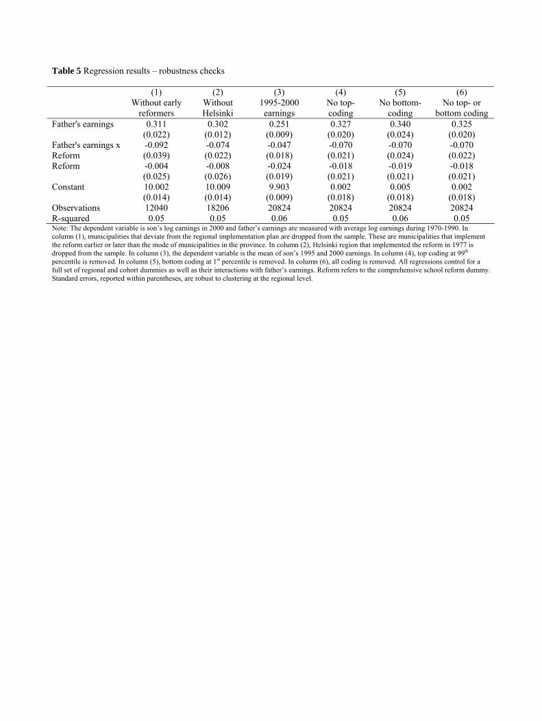
Table 5 Regression results – robustness checks (1) (2) (3) (4) (5) (6) Without early

reformers Without Helsinki

1995-2000 earnings

No top-coding

No bottom-coding

No top- or bottom coding

Father's earnings 0.311 0.302 0.251 0.327 0.340 0.325 (0.022) (0.012) (0.009) (0.020) (0.024) (0.020) Father's earnings x -0.092 -0.074 -0.047 -0.070 -0.070 -0.070 Reform (0.039) (0.022) (0.018) (0.021) (0.024) (0.022) Reform -0.004 -0.008 -0.024 -0.018 -0.019 -0.018 (0.025) (0.026) (0.019) (0.021) (0.021) (0.021) Constant 10.002 10.009 9.903 0.002 0.005 0.002 (0.014) (0.014) (0.009) (0.018) (0.018) (0.018) Observations 12040 18206 20824 20824 20824 20824 R-squared 0.05 0.05 0.06 0.05 0.06 0.05 Note: The dependent variable is son’s log earnings in 2000 and father’s earnings are measured with average log earnings during 1970-1990. In column (1), municipalities that deviate from the regional implementation plan are dropped from the sample. These are municipalities that implement the reform earlier or later than the mode of municipalities in the province. In column (2), Helsinki region that implemented the reform in 1977 is dropped from the sample. In column (3), the dependent variable is the mean of son’s 1995 and 2000 earnings. In column (4), top coding at 99th percentile is removed. In column (5), bottom coding at 1st percentile is removed. In column (6), all coding is removed. All regressions control for a full set of regional and cohort dummies as well as their interactions with father’s earnings. Reform refers to the comprehensive school reform dummy. Standard errors, reported within parentheses, are robust to clustering at the regional level.

Table 6 Regression results - pairwise comparisons a) By cohorts 1960 1961 1962 1963 1964 1965 1960 1961 -0.031 (0.098) 1962 -0.101 0.007 (0.069) (0.085) 1963 -0.195 -0.162 -0.151 (0.063) (0.065) (0.076) 1964 0.029 0.036 -0.007 0.020 (0.068) (0.062) (0.063) (0.080) 1965 -0.086 -0.111 -0.006 -0.162 -0.145 (0.101) (0.072) (0.063) (0.066) (0.085) 1966 -0.041 0.002 -0.067 -0.183 0.079 0.002 (0.032) (0.105) (0.074) (0.066) (0.071) (0.105) Note: Numbers are the coefficients of the interaction of the reform dummy and father’s earnings in differences-in-differences regressions that are conducted pairwise by cohorts. Standard errors are reported within parentheses. b) By regions 1972 1973 1974 1975 1976 1972 1973 0.070 (0.091) 1974 -0.016 -0.037 (0.068) (0.081) 1975 -0.039 -0.112 -0.162 (0.065) (0.065) (0.075) 1976 -0.098 -0.072 -0.169 0.017 (0.064) (0.057) (0.058) (0.077) 1977 -0.017 -0.067 -0.019 0.102 -0.178 (0.087) (0.071) (0.066) (0.073) (0.097) Note: Numbers are the coefficients of the interaction of the reform dummy and father’s earnings in differences-in-differences regressions that are conducted pairwise by regions. Standard errors are reported within parentheses.

Table 7 The effect of the reform on son’s earnings by father’s income quintiles (1) (2) (3) (4) (5) 1st quintile of

father’s earnings 2nd quintile of father’s earnings

3rd quintile of father’s earnings

4th quintile of father’s earnings

5th quintile of father’s earnings

Reform 0.036 0.038 -0.037 -0.051 -0.080 (0.045) (0.040) (0.038) (0.041) (0.048) Constant 9.770 9.918 10.037 10.096 10.294 (0.025) (0.022) (0.021) (0.022) (0.026) Observations 4165 4165 4165 4165 4164 R-squared 0.00 0.00 0.01 0.00 0.01 Note: Coefficients of the reform dummy in regressions where son’s log earnings are regressed on the reform, cohort, and regional dummies and the data are split by the quintiles of the fathers’ earnings distribution. Standard errors are reported in parentheses.