CBO’s Cost Estimates

Congressional Budget Office

CBO’s Cost Estimates

Center on Budget and Policy Priorities Washington, D.C.

October 29, 2015

Wendy Edelberg Assistant Director, Macroeconomic Analysis

Teri Gullo Assistant Director, Budget Analysis For additional information, see Congressional Budget Office, “Dynamic Analysis,” www.cbo.gov/topics/dynamic-analysis.

http://www.cbo.gov/topics/dynamic-analysis

1 CO NGR ES S IO NA L B UDGE T O F F IC E

Overview

■ CBO’s conventional estimates

■ New requirement for dynamic scoring

■ CBO’s approach to dynamic analysis

■ Case study: Restoring Americans’ Healthcare Freedom Reconciliation Act of 2015


Conventional Cost Estimates


The Congressional Budget and Impoundment Control Act: CBO’s Statutory Duties for Cost Estimates

■ Section 202—CBO assists committees and members. – Budget committees – Appropriations, Finance, Ways and Means – Other committees – Individual members (by providing information compiled in assisting

budget committees)

■ Section 402—Formal cost estimates must be prepared when bills are reported by full authorizing committees.

■ Section 308—Other analyses. – PAYGO estimates (as requested by budget committees)

■ CBO’s cost estimates are advisory.


Contents of Formal Cost Estimates

■ An assessment of the budgetary impact of legislation in the context of current law

■ How enactment or implementation of a bill would affect: – Budget authority (legal authority to enter into obligations) – Outlays (cash disbursements) – Authorization levels (funding subject to future appropriations) – Revenues (taxes and other governmental receipts); analyzed by CBO

and the Joint Committee on Taxation (JCT)

■ Estimates also include: – The basis of the estimate – Mandate statements – A PAYGO table – Staff contacts


Formal Estimates and How to Find Them

■ CBO completes 400 to 600 formal estimates each year.

■ All formal estimates are posted on www.cbo.gov and are searchable by bill number, budget function, committee, and key word.


Informal Reviews

■ CBO receives thousands of requests for informal reviews each year.

■ Order of priority: – Bills and amendments during the rules or appropriation process – Requests by budget committee, leadership, committees of jurisdiction – Bills prior to committee markup – Legislative proposals prior to introduction

■ Informal reviews are preliminary.


Informal Reviews (Continued)

■ The mode of response depends on competing priorities and the complexity of the analysis.

■ Reviews focus on direct spending and effects on revenue.

■ CBO ensures confidentiality for proposals that are not yet public.


Behavioral Responses in Conventional Cost Estimates

■ If proposed policies would affect people’s behavior in ways that would affect the budget, those effects are incorporated in CBO’s conventional estimates. – Change in crop production from adopting new farm policies – Likelihood that people would take up government benefits when

policies change – Quantity of health care services that would be provided if Medicare’s

payment rates were changed

■ By long-standing convention, CBO’s cost estimates generally have not reflected changes in behavior that would affect total output in the economy, such as any changes in labor supply or private investment resulting from changes in fiscal policy.


The New Requirement for Dynamic Scoring


Requirements Under the 2016 Budget Resolution

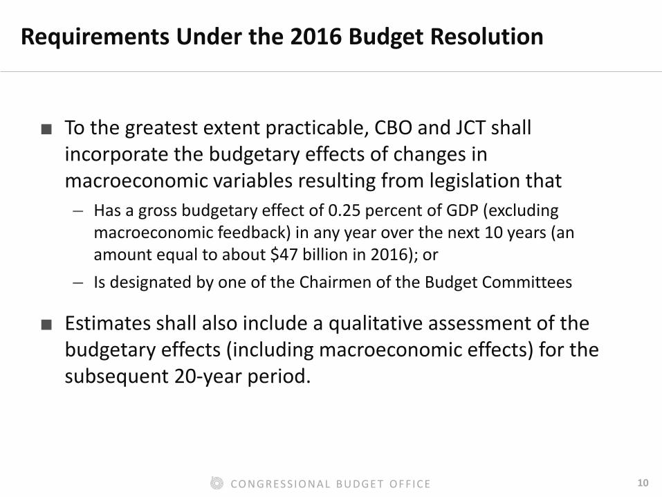
■ To the greatest extent practicable, CBO and JCT shall incorporate the budgetary effects of changes in macroeconomic variables resulting from legislation that – Has a gross budgetary effect of 0.25 percent of GDP (excluding

macroeconomic feedback) in any year over the next 10 years (an amount equal to about $47 billion in 2016); or

– Is designated by one of the Chairmen of the Budget Committees

■ Estimates shall also include a qualitative assessment of the budgetary effects (including macroeconomic effects) for the subsequent 20-year period.


Requirements Under the 2016 Budget Resolution (Continued)

■ Appropriation acts are excluded.

■ CBO and JCT will coordinate on legislation that significantly affects both spending and tax policies.


The New Requirement Extends Previous Analyses by CBO

CBO has routinely produced estimates of the macroeconomic effects of fiscal policies and of the feedback from those macroeconomic changes to the federal budget:

■ Analysis of the President’s budget

■ Annual long-term budget and economic outlook

■ Analyses of illustrative fiscal policy scenarios


The New Requirement Extends Previous Analyses by CBO (Continued)

■ CBO has generally not produced estimates for specific legislation prior to the 2016 budget resolution (one exception is S. 744, the Border Security, Economic Opportunity, and Immigration Modernization Act).

■ Because the bill would have significantly increased the size of the U.S. labor force, CBO and JCT incorporated in the cost estimate their projections of the direct effects of the act on the U.S. population, employment, and taxable compensation.

■ CBO separately published an analysis of additional economic effects and their feedback to the budget.


Recent Acts That CBO Has Analyzed Using Dynamic Scoring

■ Proposal to repeal the Affordable Care Act

■ Tax Relief Extension Act of 2015 (estimated by the staff of the Joint Committee on Taxation)

■ Restoring Americans’ Healthcare Freedom Reconciliation Act of 2015


CBO’s Approach to Dynamic Analysis


CBO’s Approach to Analyzing Economic Effects of Fiscal Policies

■ Short term: Changes in fiscal policies affect the overall economy primarily by influencing the demand for goods and services by consumers, businesses, and governments, which leads to changes in output relative to potential (maximum sustainable) output.

■ Long term: Changes in fiscal policies affect output primarily by altering national saving, foreign investment in the U.S., federal investment, and people’s incentives to work and save, as well as businesses’ incentives to invest, thereby changing potential output.


Central Estimates and Ranges

■ CBO’s estimates of those effects are based on parameters such as the extent to which national saving is altered by changes in fiscal policies.

■ In most cases, CBO estimates the economic effects (and feedback to the budget) using a range of parameter estimates reflecting the consensus in the economic literature.

■ To arrive at its estimate of the economic effects, CBO uses the central estimates for those parameters.


Short-Term Effects From Changes in Demand

■ Direct contributions to aggregate demand stem from changes in purchases by federal agencies and those who receive federal payments and pay taxes.

■ The change in output for each dollar of direct contribution to demand (the demand multiplier) varies with the response of monetary policy.

■ In CBO’s estimates of indirect effects: – When the monetary policy response is likely to be limited, the demand

multiplier over four quarters ranges from 0.5 to 2.5, with a central estimate of 1.5.

– When the monetary policy response is likely to be stronger, the demand multiplier over four quarters ranges from 0.4 to 1.9, with a central estimate of 1.2; over eight quarters, it ranges from 0.2 to 0.8, with a central estimate of 0.5.


Short-Term Effects From Changes in Labor Supply

■ Effects on the supply of labor lead to changes in employment, depending on the amount of slack in the labor market.


Long-Term Effects

■ CBO uses two models of potential output to estimate the effects of changes in fiscal policies on the overall economy over the long term. – Solow-type growth model – Life-cycle growth model

■ Potential output depends on: – Amount and quality of labor and capital (which depend on work,

saving, and investment) – Productivity of the labor and capital inputs (which depends in part on

federal investment) – Amount of national saving (which depends in part on federal

borrowing)


The Role of Expectations About Fiscal Policy: Solow-Type Growth Model

■ People base their decisions about working and saving primarily on current economic conditions, including government policies.

■ Decisions reflect people’s anticipation of future policies in a general way but not their responses to specific future developments.


The Role of Expectations About Fiscal Policy: Life-Cycle Growth Model

■ People make choices about working and saving in response to both current economic conditions and their explicit expectations of future economic conditions.

■ The model requires specification of future fiscal policies that put federal debt on a sustainable path over the long run because forward-looking households would not hold government bonds if the households expected that debt as a percentage of GDP would rise without limit.


How Labor Supply Responds to Changes in Fiscal Policy in the Solow-Type Growth Model

■ The overall effects of a policy change on the labor supply can be expressed as an elasticity, which is the percentage change in the labor supply resulting from a 1 percent change in after-tax income.

■ Substitution effect: Increased after-tax compensation for an additional hour of work makes work more valuable relative to other uses of a person’s time.

■ Income effect: Increased after-tax income from a given amount of work allows people to maintain the same standard of living while working fewer hours.


How Labor Supply Responds to Changes in Fiscal Policy in the Solow-Type Growth Model (Continued)

■ CBO’s central estimate corresponds to an earnings-weighted total wage elasticity for all earners of 0.19 (composed of a substitution elasticity of 0.24 and an income elasticity of -0.05).

■ For some proposals, income and substitution effects may not offset each other (for example, if the proposal would increase after-tax wages but reduce income).

■ CBO estimates that the substitution elasticity could range from a low estimate of about 0.16 to a high estimate of about 0.32; the income elasticity could range from about -0.10 to about 0.


Other Key Aspects of the Solow-Type Growth Model

■ When the deficit increases by one dollar, private saving is estimated to rise by 43 cents (national saving falls by 57 cents), and net capital inflows rise by 24 cents, ultimately leaving a decline of 33 cents in investment. – Range of estimates: The decline in investment ranges from 15 cents to

50 cents.

■ Additional federal investment is estimated to yield half of the typical return on investment completed by the private sector. – The range of estimates goes from no return on investment to the

typical return on investment completed by the private sector.


Key Aspects of the Life-Cycle Growth Model

■ Labor supply and private saving are influenced by the current values and future anticipated values of the after-tax rate of return on saving, the after-tax wage, and households’ disposable income, among other factors.

■ The elasticity with respect to a one-time temporary change in wages (the so-called Frisch elasticity) is 0.40, according to CBO’s central estimates, with a range from 0.27 to 0.53. – Frisch elasticity is calibrated to be consistent with CBO’s estimate of the

total wage elasticity.

■ Because of the uncertainty that households face about their future income, households in the life-cycle growth model take the precaution of holding additional savings as a buffer against potential drops in income.


Range of Estimates Within the Life-Cycle Growth Model

■ CBO models two sets of assumptions about the openness of the economy: a small open economy, in which wages and interest rates are determined by world markets, and a version of a closed economy, in which wages and interest rates are determined domestically.

■ Because the model is forward-looking, it requires offsetting policy changes that eventually stabilize government debt (closure rules); beginning in 15 years, those policies would be phased in over 10 years. CBO models two sets of assumptions: – Reduced spending (half from government purchases and half from

transfers) – Increased taxes (half from marginal rate changes and half in lump-sum

amounts)

■ Both closure rules are reported, and results generally are similar.


Uncertainty in Budgetary Outcomes

■ When practicable and informative, CBO will report the estimated range of budgetary outcomes owing to the uncertainty of macroeconomic effects.

■ CBO needs to consider the uncertainty regarding feedback relative to the ability to describe uncertainty of the conventional cost estimate.

■ CBO will report the range of Solow-type growth model estimates. – Differences between Solow-type growth model results and those of the

life-cycle growth model reflect model uncertainty rather than parameter uncertainty, making interpretation difficult.


Uncertainty in Budgetary Outcomes (Continued)

■ The likelihood that all parameters would simultaneously be at the ends of their ranges is smaller than the likelihood that any single parameter would be at the end of its range. – CBO focuses on uncertainty about the two parameters that have the

largest budgetary effects. – CBO examines estimates resulting from cases in which two parameters

are at the ends of their ranges and other parameters are equal to central estimates.

■ CBO will report cases that show the most favorable and least favorable budgetary outcomes.


Presentation of Macroeconomic Analyses in Cost Estimates

■ The presentation will probably evolve over time as CBO learns what is most useful.

■ Estimates will show all of the information that traditionally would be included if macroeconomic effects were not incorporated and will identify the macroeconomic effects separately.

■ Estimates will provide information related to the uncertainty of the macroeconomic effects.


Case Study: H.R. 3762, Restoring Americans’

Healthcare Freedom Reconciliation Act of 2015


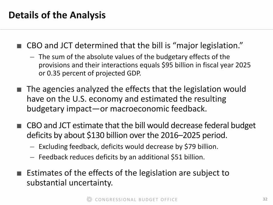
Details of the Analysis

■ CBO and JCT determined that the bill is “major legislation.” – The sum of the absolute values of the budgetary effects of the

provisions and their interactions equals $95 billion in fiscal year 2025 or 0.35 percent of projected GDP.

■ The agencies analyzed the effects that the legislation would have on the U.S. economy and estimated the resulting budgetary impact—or macroeconomic feedback.

■ CBO and JCT estimate that the bill would decrease federal budget deficits by about $130 billion over the 2016–2025 period. – Excluding feedback, deficits would decrease by $79 billion. – Feedback reduces deficits by an additional $51 billion.

■ Estimates of the effects of the legislation are subject to substantial uncertainty.


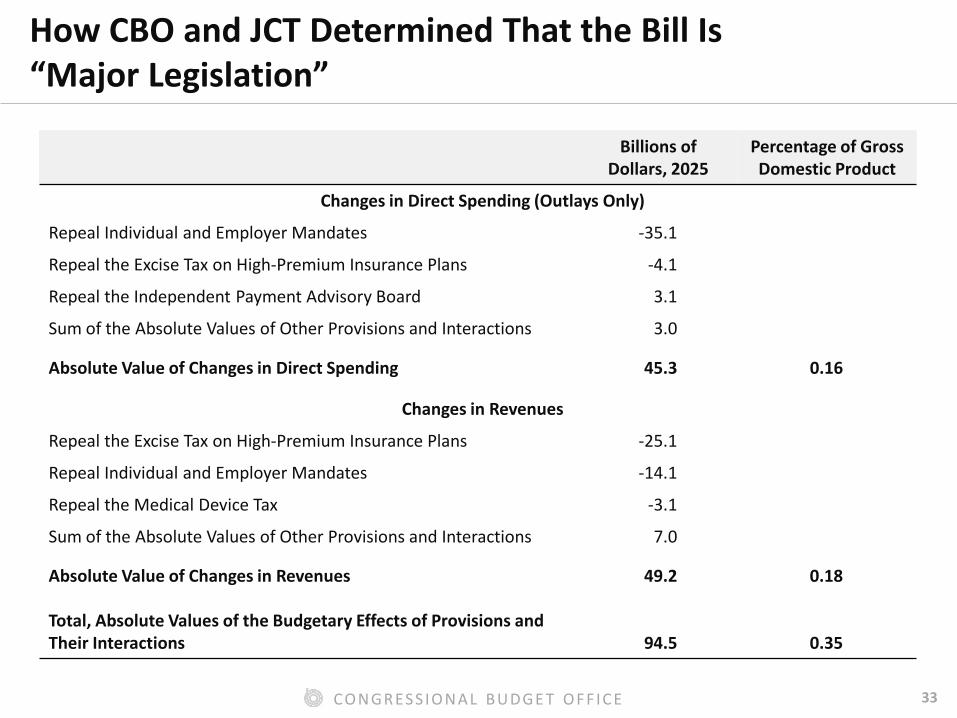
How CBO and JCT Determined That the Bill Is “Major Legislation”

Billions of Dollars, 2025

Percentage of Gross Domestic Product

Changes in Direct Spending (Outlays Only)

Repeal Individual and Employer Mandates -35.1

Repeal the Excise Tax on High-Premium Insurance Plans -4.1

Repeal the Independent Payment Advisory Board 3.1

Sum of the Absolute Values of Other Provisions and Interactions 3.0

Absolute Value of Changes in Direct Spending 45.3 0.16

Changes in Revenues

Repeal the Excise Tax on High-Premium Insurance Plans -25.1

Repeal Individual and Employer Mandates -14.1

Repeal the Medical Device Tax -3.1

Sum of the Absolute Values of Other Provisions and Interactions 7.0

Absolute Value of Changes in Revenues 49.2 0.18

Total, Absolute Values of the Budgetary Effects of Provisions and Their Interactions 94.5 0.35


Budgetary Effects of H.R. 3762

The largest budgetary effects of enacting the legislation would stem from:

■ Repealing provisions of the Affordable Care Act that require most people to obtain health insurance coverage and large employers to offer their employees health insurance coverage that meets specified standards or pay penalties

■ Repealing the federal excise taxes imposed on the sale of medical devices and on certain employer-provided health coverage with premiums above specified amounts


Economic Effects of H.R. 3762

■ From 2021 to 2025, the bill would boost GDP by about 0.2 percent, on average, relative to current-law projections.

■ The bill would increase the supply of labor by increasing incentives to work.

■ The bill would increase the size of the capital stock by increasing labor supply (which makes capital more productive) and by decreasing federal borrowing (which increases the money available for investment).


Short-Term Economic Effects of H.R. 3762

■ The bill would have lesser effects on output in the next few years than would occur later in the coming decade.

■ Aggregate demand would be slightly lower in the short run.

■ There would be a growing boost over time to the number of hours worked (as more people responded to the increase in incentives to work).


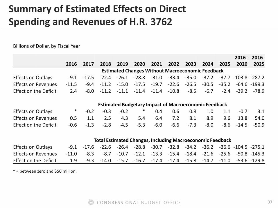
Summary of Estimated Effects on Direct Spending and Revenues of H.R. 3762

2016 2017 2018 2019 2020 2021 2022 2023 2024 2025 2016-2020

2016-2025

Estimated Changes Without Macroeconomic Feedback Effects on Outlays -9.1 -17.5 -22.4 -26.1 -28.8 -31.0 -33.4 -35.0 -37.2 -37.7 -103.8 -287.2 Effects on Revenues -11.5 -9.4 -11.2 -15.0 -17.5 -19.7 -22.6 -26.5 -30.5 -35.2 -64.6 -199.3 Effect on the Deficit 2.4 -8.0 -11.2 -11.1 -11.4 -11.4 -10.8 -8.5 -6.7 -2.4 -39.2 -78.9

Estimated Budgetary Impact of Macroeconomic Feedback Effects on Outlays * -0.2 -0.3 -0.2 * 0.4 0.6 0.8 1.0 1.1 -0.7 3.1 Effects on Revenues 0.5 1.1 2.5 4.3 5.4 6.4 7.2 8.1 8.9 9.6 13.8 54.0 Effect on the Deficit -0.6 -1.3 -2.8 -4.5 -5.3 -6.0 -6.6 -7.3 -8.0 -8.6 -14.5 -50.9

Total Estimated Changes, Including Macroeconomic Feedback Effects on Outlays -9.1 -17.6 -22.6 -26.4 -28.8 -30.7 -32.8 -34.2 -36.2 -36.6 -104.5 -275.1 Effects on Revenues -11.0 -8.3 -8.7 -10.7 -12.1 -13.3 -15.4 -18.4 -21.6 -25.6 -50.8 -145.3 Effect on the Deficit 1.9 -9.3 -14.0 -15.7 -16.7 -17.4 -17.4 -15.8 -14.7 -11.0 -53.6 -129.8

* = between zero and $50 million.

Billions of Dollar, by Fiscal Year


Long-Term Effects of H.R. 3762

■ CBO and JCT estimate that enacting the bill would increase deficits in the decades after 2026, with or without macroeconomic feedback.

■ Excluding macroeconomic feedback, the loss of revenues from the repeal of the excise tax on certain high-premium health insurance plans would more than offset the savings from other provisions of the bill, causing an increase in budget deficits soon after 2025.

■ Macroeconomic feedback is estimated to ultimately increase deficits despite the boost to incentives to work; in particular, the increase in deficits that would occur after 2025 (excluding macroeconomic feedback) would put upward pressure on interest rates and interest payments.

Government & Nonprofit

CBO’s Cost Estimates