The role of physical modelling of atmospheric

dispersionAlan Robins, University of Surrey

Computer modelling

Activities:

Educate

Provide data

Develop knowledge

Solve practical questions

The Alan G. Davenport Symposium

UWO, June, 2002

Dispersion Modelling

What did the wind tunnel ever do for us?

Major contributions by topic area:

Basic dispersion processes Complex terrain

Plume rise and entrainment Dense gas dispersion

Building effects Concentration fluctuations

Urban boundary layer Convective boundary layer

… and water tanks ....

Methodologies

Examples:

Plume rise + buildings

Leaks and losses

Urban dispersion

Dense gases

Inverse modelling

Density ratio, speed ratio, Richardson number

ro

r

Wo

U

gH

U 2Þ

Ufs

Uwt

= e

e , the length scale ratio

'Relaxed' scaling

dimensionless momentum and buoyancy fluxes

roW

o

2

rU 2

gDrWoH

rU 3Þ

Ufs

Uwt

= ea

m

afs

æ

èç

ö

ø÷

1/2

1-afs

1-am

é

ë

êê

ù

û

úú

1/2

a , the density ratio

Methodology

Wind tunnel

Neutral

Slightly stable

Slightly unstable

Water tank

Neutral

Very stable

Very unstable

Source modellingInflow simulation

Implications

Working section

H ~1 m working section length ~ 10 - 20 m; height ~ 1.5 to 2 m; width at least two

to three times the height ~ 4 m; wind speed range 0.5 to 5 ms-1.

boundary layer simulation emissions simulation/model maximum glc

physical model

plume rise &

spreadH

h

Dh

U(z), u'(z), etc.

10 H 5 - 10 H

Boundary layer simulation

Standard methods for neutral conditions

– vorticity generators, rough surface.

No standard approaches for stable and

unstable conditions.

Fast

FFID system

Chilled water

supply ~ 10˚CTwin

fans

20 x 3.5 x 1.5 m

working section

0 - 3 ms-1

Inlet and heater section

15 layers 400 kW capacity

ambient to ~ 80˚C

Rough wall

cooled ~ 15˚C

heated ~ 100˚C

Mechanical simulation

devices & rough wall

Heat

exchanger

Turntable

Heater control

with thermistor

feedback

Gas

supplies

Run control

system

Computer control, data

collection & data analysis

Thermistor

systems

Speed

control

Traverse and

turntable

control

LDA, PIV, hot

wire, cold wire,

web-cams etc

Source

Example 1: Buoyant plume and buildings

0.0

0.1

0.2

0.3

0 5 10 15 20 25

Dim

ensi

on

less

co

nce

ntr

atio

n

Wind speed at 10m, m/s

Maximum glc at

500 - 600m downwind

Wind tunnel, density ratio = 0.30

= 0.37

= 0.75

= 0.92

Field data, density ratio 0.83

H = 54m,W

o=12ms-1, Q

H= 5.8 MW , DT = 60 K

Example 2: Leaks and losses

Chemical process plant

---

an example of a

complex site that, in

turn, creates complex

flow and dispersion

conditions in short

range

---

conditions that are not

easily parameterised.

Wake flows

Characteristics of the

wake flow downwind of

obstacles of different

porosities.

There is often a need to

interpret measurements

of wind speed and

pollutant concentration in

such flows to detect and

quantify loss rates.

Interpretation

Direct application of results is sometimes feasible …

… more likely that the outcome of wind tunnel work is integrated into a

dispersion model to allow extrapolation to all wind/weather conditions

… a process model is built to link the experiments and the model.

That might be as simple as a virtual source definition or as complex as a

full, near-field dispersion module.

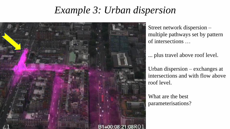
Example 3: Urban dispersion

Street network dispersion –

multiple pathways set by pattern

of intersections …

... plus travel above roof level.

Urban dispersion – exchanges at

intersections and with flow above

roof level.

What are the best

parameterisations?

Concentration decay – passive release

Street network dispersion

– multiple pathwaysCombined wind tunnel and field data from

London (DAPPLE) led to a robust correlation:

confirmed and refined by later wind tunnel

work using a 1:350 scale model of central

Paris.

Note that the blue symbols represent upwind

dispersion.

C*

R/H

Upper bound dimensionless concentration

as function of separation.

CU (H )H 2

Q= 12

R

H

æ

èçö

ø÷

-2

Source-receptor relationships

Contributions from sources in and around

Marylebone Road to concentration observed

at the AURN site.

C* = CUH2/Q

Regions responsible for 80% of the

concentration at the AURN site:

180˚, -45˚, -90˚, 45˚.

Urban areas and dense gas dispersion

Source at

ground level

Carbon dioxide

Q = 50 litre min-1

U = 1 ms-1

Extensive

upwind and

lateral spread

from the

source.

How is chanelling (wind along major, straight street) to be treated?

How in this

parameterised?

Inverse modelling

Use data series to

determine source

properties (Q, To, x, y).

Understand response to

data quality; e.g.

sampling time.

How soon can a reliable

estimate be attained?

Four detectors returning C(t).

Example: response to averaging time in open terrain

-50.0

0.0

50.0

100.0

150.0

200.0

10 100 1000 10000 100000 1000000

So

urc

e p

osi

tio

n, x

, m

Averaging time, s

power law spread

linear spread

This is performance in a

simple boundary layer,

where the dispersion model

can be made accurate.

Near obstacles, or with

dense gas or buoyant

plumes, the errors in the

dispersion model dominate.

Search for source properties

that minimise mean square

error in predictions.

… to summarise …

Wind tunnel simulation - a proven technology for research and practice

Neutral, slightly stable, slightly unstable conditions; stable/unstable in water tank

Stand alone or used in conjunction with models

LES makes the most fruitful combination

Current interests at EnFlo include

the urban environment indoor and out MAGIC

hazardous gas dispersion/inverse modelling MODITIC

a.robins@surrey.ac.uk

Automation an essential operational requirement