Embed Size (px)
Citation preview

Are South Hills Crossbills Declining with Increasing Temperatures?
Julie Hart Master’s Defense
Zoology & Physiology 29 April 2013

INTRODUCTION � ABUNDANCE � SURVIVAL � CLIMATE � CONES � CONCLUSIONS
EXTINCTION RISK
..............................................................
Extinction risk from climate changeChris D. Thomas1, Alison Cameron1, Rhys E. Green2, Michel Bakkenes3,Linda J. Beaumont4, Yvonne C. Collingham5, Barend F. N. Erasmus6,Marinez Ferreira de Siqueira7, Alan Grainger8, Lee Hannah9,Lesley Hughes4, Brian Huntley5, Albert S. van Jaarsveld10,Guy F. Midgley11, Lera Miles8*, Miguel A. Ortega-Huerta12,A. Townsend Peterson13, Oliver L. Phillips8 & Stephen E. Williams14
1Centre for Biodiversity and Conservation, School of Biology, University of Leeds,Leeds LS2 9JT, UK2Royal Society for the Protection of Birds, The Lodge, Sandy, BedfordshireSG19 2DL, UK, and Conservation Biology Group, Department of Zoology,University of Cambridge, Downing Street, Cambridge CB2 3EJ, UK3National Institute of Public Health and Environment, P.O. Box 1,3720 BA Bilthoven, The Netherlands4Department of Biological Sciences, Macquarie University, North Ryde, 2109,NSW, Australia5University of Durham, School of Biological and Biomedical Sciences, South Road,Durham DH1 3LE, UK6Animal, Plant and Environmental Sciences, University of the Witwatersrand,Private Bag 3, WITS 2050, South Africa7Centro de Referencia em Informacao Ambiental, Av. Romeu Tortima 228,Barao Geraldo, CEP:13083-885, Campinas, SP, Brazil8School of Geography, University of Leeds, Leeds LS2 9JT, UK9Center for Applied Biodiversity Science, Conservation International,1919 M Street NW, Washington, DC 20036, USA10Department of Zoology, University of Stellenbosch, Private Bag X1,Stellenbosch 7602, South Africa11Climate Change Research Group, Kirstenbosch Research Centre, NationalBotanical Institute, Private Bag x7, Claremont 7735, Cape Town, South Africa12Unidad Occidente, Instituto de Biologıa, Universidad Nacional Autonoma deMexico, Mexico, D.F. 04510 Mexico13Natural History Museum and Biodiversity Research Center, University ofKansas, Lawrence, Kansas 66045 USA14Cooperative Research Centre for Tropical Rainforest Ecology, School of TropicalBiology, James Cook University, Townsville, QLD 4811, Australia
* Present address: UNEP World Conservation Monitoring Centre, 219 Huntingdon Road, Cambridge
CB3 0DL, UK
.............................................................................................................................................................................
Climate change over the past,30 years has produced numerousshifts in the distributions and abundances of species1,2 and hasbeen implicated in one species-level extinction3. Using projec-tions of species’ distributions for future climate scenarios, weassess extinction risks for sample regions that cover some 20% ofthe Earth’s terrestrial surface. Exploring three approaches inwhich the estimated probability of extinction shows a power-law relationship with geographical range size, we predict, onthe basis of mid-range climate-warming scenarios for 2050, that15–37% of species in our sample of regions and taxa will be‘committed to extinction’. When the average of the three methodsand two dispersal scenarios is taken, minimal climate-warmingscenarios produce lower projections of species committed toextinction (,18%) than mid-range (,24%) and maximum-change (,35%) scenarios. These estimates show the importanceof rapid implementation of technologies to decrease greenhousegas emissions and strategies for carbon sequestration.
The responsiveness of species to recent1–3 and past4,5 climatechange raises the possibility that anthropogenic climate changecould act as a major cause of extinctions in the near future, with theEarth set to become warmer than at any period in the past 1–40Myr(ref. 6). Here we use projections of the future distributions of1,103 animal and plant species to provide ‘first-pass’ estimates ofextinction probabilities associated with climate change scenarios for2050.
For each species we use the modelled association between currentclimates (such as temperature, precipitation and seasonality)and present-day distributions to estimate current distributional
areas7–12. This ‘climate envelope’ represents the conditions underwhich populations of a species currently persist in the face ofcompetitors and natural enemies. Future distributions are esti-mated by assuming that current envelopes are retained and can beprojected for future climate scenarios7–12. We assume that a specieseither has no limits to dispersal such that its future distributionbecomes the entire area projected by the climate envelope model orthat it is incapable of dispersal, in which case the new distribution isthe overlap between current and future potential distributions (forexample, species with little dispersal or that inhabit fragmentedlandscapes)11. Reality for most species is likely to fall between theseextremes.We explore three methods to estimate extinction, based on the
species–area relationship, which is a well-established empiricalpower-law relationship describing how the number of speciesrelates to area (S ¼ cAz, where S is the number of species, A isarea, and c and z are constants)13. This relationship predictsadequately the numbers of species that become extinct or threat-ened when the area available to them is reduced by habitatdestruction14,15. Extinctions arising from area reductions shouldapply regardless of whether the cause of distribution loss is habitatdestruction or climatic unsuitability.Because climate change can affect the distributional area of each
species independently, classical community-level approaches needto be modified (see Methods). In method 1 we use changes in thesummed distribution areas of all species. This is consistent with thetraditional species–area approach: on average, the destruction ofhalf of a habitat results in the loss of half of the distribution areasummed across all species restricted to that habitat. However, thisanalysis tends to be weighted towards species with large distribu-tional areas. To address this, in method 2 we use the averageproportional loss of the distribution area of each species to estimatethe fraction of species predicted to become extinct. This approach isfaithful to the species–area relationship because halving thehabitat area leads on average to the proportional loss of halfthe distribution of each species. Method 3 considers the extinc-tion risk of each species in turn. In classical applications of thespecies–area approach, the fraction of species predicted tobecome extinct is equivalent to the mean probability of extinc-tion per species. Thus, in method 3 we estimate the extinctionrisk of each species separately by substituting its area loss in thespecies–area relationship, before averaging across species (seeMethods). Our conclusions are not dependent on which ofthese methods is used. We use z ¼ 0.25 in the species–arearelationship throughout, given its previous success in predictingproportions of threatened species14,15, but our qualitative con-clusions are not dependent on choice of z (SupplementaryInformation). As there are gaps in the data (not all dispersal/climatescenarios were available for each region), a logit–linear model isfitted to the extinction risk data to produce estimates for missingvalues in the extinction risk table (Table 1). Balanced estimates ofextinction risk, averaged across all data sets, can then be calculatedfor each scenario.For projections of maximum expected climate change, we esti-
mate species-level extinction across species included in the study tobe 21–32% (range of the three methods) with universal dispersal,and 38–52% for no dispersal (Table 1). For projections ofmid-rangeclimate change, estimates are 15–20% with dispersal and 26–37%without dispersal (Table 1). Estimates for minimum expectedclimate change are 9–13% extinction with dispersal and 22–31%without dispersal. Projected extinction varies between parts of theworld and between taxonomic groups (Table 1), so our estimates areaffected by the data available. The species–area methods differ fromone another by up to 1.41-fold (method 1 versus method 3) inestimated extinction, whereas the two dispersal scenarios producea 1.98-fold difference, and the three climate scenarios generate2.05-fold variation.
letters to nature
NATURE |VOL 427 | 8 JANUARY 2004 | www.nature.com/nature 145© 2004 Nature Publishing Group

South Hills (Type 9)
A F L P V A R I A T I O N I N C R O S S B I L L S 1881
© 2006 Blackwell Publishing Ltd, Molecular Ecology, 15, 1873–1887
nonoverlapping clusters when the analysis was restrictedto red crossbills.
Only three of nine comparisons of different geographicsamples within call types revealed significant geneticdifferentiation, which contrasts with the relatively highnumber of comparisons that were significant between calltypes (25 of 28 comparisons; Fisher’s exact test, P = 0.002).The significant within-call-type comparisons were betweencall type 2 in the Black Hills, South Dakota, and both theSandia Mountains, New Mexico (FST = 0.057, P < 0.05), andthe Bears Paw Mountains, Montana (FST = 0.041, P < 0.05),and between call type 1 from North Carolina and Virginia(FST = 0.13, P < 0.05). amova examining variation among
samples of call type 2 from different geographic locations(Fig. 1) indicates that the vast majority of variation isfound within location (97%) but that a significant amountof variation (3.1%) was due to differences among locations,which was lower than the 7% explained by differencesamong call types (Table 3). Finally, different geographicsamples within call types 1, 2, and 5 grouped togetherin the upgma dendrogram (Fig. 4), suggesting geneticcontinuity within these call types, whereas the twogeographically separate samples of call type 7 did notgroup together (Fig. 4), perhaps not surprisingly as calltype 7 did not differ significantly from call types 3, 4, and6 based on FST (Table 4).
Fig. 4 upgma phylogram reflecting relative genetic distances based on pairwise estimates of Nei’s D among different recognized speciesincluded in this study and eight call types of the red crossbill complex including samples from two geographic samples of call types 1, 5,and 7, and four geographic samples of call type 2 (BP, Bears Paw Mountains; NM, New Mexico; BH, Black Hills; LR, Little Rocky Mountains,with the samples taken in 2000 and 2001 distinguished as LRa and LRb, respectively). Values at the nodes represent bootstrap support basedon 1000 replicates; values < 50% are not shown. A representative head and, where known, a cone of the conifer on which each crossbillspecializes is shown. Heads and cones are from figures in Benkman (1987b, 1999), Parchman & Benkman (2002) and Farjon & Styles (1997),with bill sizes and cones altered to reflect relative sizes among the different crossbills and conifers, respectively. Cones from top to bottomare: Pinus occidentalis, Picea mariana, Pinus contorta latifolia from South Hills, Pinus ponderosa scopulorum, Pinus contorta latifolia, Tsugaheterophylla, Pseudotsuga menziesii menziesii, and Picea rubens. Call type 4 is associated with Pseudotsuga m. menziesii.
Type 2
Type 3
Type 4
Type 5
Type 1
A F L P V A R I A T I O N I N C R O S S B I L L S 1881
© 2006 Blackwell Publishing Ltd, Molecular Ecology, 15, 1873–1887
nonoverlapping clusters when the analysis was restrictedto red crossbills.
Only three of nine comparisons of different geographicsamples within call types revealed significant geneticdifferentiation, which contrasts with the relatively highnumber of comparisons that were significant between calltypes (25 of 28 comparisons; Fisher’s exact test, P = 0.002).The significant within-call-type comparisons were betweencall type 2 in the Black Hills, South Dakota, and both theSandia Mountains, New Mexico (FST = 0.057, P < 0.05), andthe Bears Paw Mountains, Montana (FST = 0.041, P < 0.05),and between call type 1 from North Carolina and Virginia(FST = 0.13, P < 0.05). amova examining variation among
samples of call type 2 from different geographic locations(Fig. 1) indicates that the vast majority of variation isfound within location (97%) but that a significant amountof variation (3.1%) was due to differences among locations,which was lower than the 7% explained by differencesamong call types (Table 3). Finally, different geographicsamples within call types 1, 2, and 5 grouped togetherin the upgma dendrogram (Fig. 4), suggesting geneticcontinuity within these call types, whereas the twogeographically separate samples of call type 7 did notgroup together (Fig. 4), perhaps not surprisingly as calltype 7 did not differ significantly from call types 3, 4, and6 based on FST (Table 4).
Fig. 4 upgma phylogram reflecting relative genetic distances based on pairwise estimates of Nei’s D among different recognized speciesincluded in this study and eight call types of the red crossbill complex including samples from two geographic samples of call types 1, 5,and 7, and four geographic samples of call type 2 (BP, Bears Paw Mountains; NM, New Mexico; BH, Black Hills; LR, Little Rocky Mountains,with the samples taken in 2000 and 2001 distinguished as LRa and LRb, respectively). Values at the nodes represent bootstrap support basedon 1000 replicates; values < 50% are not shown. A representative head and, where known, a cone of the conifer on which each crossbillspecializes is shown. Heads and cones are from figures in Benkman (1987b, 1999), Parchman & Benkman (2002) and Farjon & Styles (1997),with bill sizes and cones altered to reflect relative sizes among the different crossbills and conifers, respectively. Cones from top to bottomare: Pinus occidentalis, Picea mariana, Pinus contorta latifolia from South Hills, Pinus ponderosa scopulorum, Pinus contorta latifolia, Tsugaheterophylla, Pseudotsuga menziesii menziesii, and Picea rubens. Call type 4 is associated with Pseudotsuga m. menziesii.
INTRODUCTION � ABUNDANCE � SURVIVAL � CLIMATE � CONES � CONCLUSIONS
RED CROSSBILL
Birds of North America

SOUTH HILLS CROSSBILL
INTRODUCTION � ABUNDANCE � SURVIVAL � CLIMATE � CONES � CONCLUSIONS
Proposed species based on: • Deeper bill • Unique call type • Resident • Seasonal nesYng • Low hybridizaYon • GeneYc differenYaYon
Benkman et al. 2009, Condor

INTRODUCTION � ABUNDANCE � SURVIVAL � CLIMATE � CONES � CONCLUSIONS
STUDY AREA
South Hills: 1530 km2 in area 65 km2 lodgepole pine

INTRODUCTION � ABUNDANCE � SURVIVAL � CLIMATE � CONES � CONCLUSIONS
STUDY AREA
ElevaYon: 1277 to 2457 m

INTRODUCTION � ABUNDANCE � SURVIVAL � CLIMATE � CONES � CONCLUSIONS
PREVIOUS FINDINGS
2003 2004 2005 2006 2007 20080
50
100
150
200
250
300
350
Year
Cros
sbill
dens
ity (
indi
vidu
als/
km2 )
Year San;steban et al. 2012, Journal of Animal Ecology
63% decline R2 = 0.97, P < 0.001

HYPOTHESIS Warmer temperatures cause seroYnous cones to open and drop their seed, reducing the amount of food for crossbills and leading to their decline.
INTRODUCTION � ABUNDANCE � SURVIVAL � CLIMATE � CONES � CONCLUSIONS
Less food

RESEARCH QUESTIONS
• Is crossbill density conYnuing to decrease? • Do changes in survival account for the observed changes in density?
• Is crossbill survival related to climate? • Is cone producYvity decreasing?
INTRODUCTION � ABUNDANCE � SURVIVAL � CLIMATE � CONES � CONCLUSIONS

RESEARCH QUESTIONS
INTRODUCTION � ABUNDANCE � SURVIVAL � CLIMATE � CONES � CONCLUSIONS
• Is crossbill density conYnuing to decrease? • Do changes in survival account for the observed changes in density?
• Is crossbill survival related to climate? • Is cone producYvity decreasing?

POINT COUNTS
INTRODUCTION � ABUNDANCE � SURVIVAL � CLIMATE � CONES � CONCLUSIONS
74 points

• 10-‐minute counts with distance sampling
• 1041 birds in 6660 minutes of observaYon
• Analyzed with standard methods including a correcYon factor for detectability
• Used program DISTANCE to esYmate density
INTRODUCTION � ABUNDANCE � SURVIVAL � CLIMATE � CONES � CONCLUSIONS
POINT COUNT ANALYSIS

CROSSBILL DENSITY
INTRODUCTION � ABUNDANCE � SURVIVAL � CLIMATE � CONES � CONCLUSIONS
●
●
●
●
●
●
●
●
●
Year
Cro
ssbi
ll de
nsity
(ind
ivid
uals
km−2
)
2003 2005 2007 2009 2011
0
50
100
150
200
250
300
350
R2 = 0.98, P < 0.001
14% annual decline
277 birds/km2
71 birds/km2
75% decline

Cerulean Warbler (-‐3%)
CROSSBILL DECLINE
INTRODUCTION � ABUNDANCE � SURVIVAL � CLIMATE � CONES � CONCLUSIONS
Bicknell’s Thrush (-‐7%)
Rusty Blackbird (-‐10%)
South Hills Crossbill (-‐14%)

RESEARCH QUESTIONS
INTRODUCTION � ABUNDANCE � SURVIVAL � CLIMATE � CONES � CONCLUSIONS
• Is crossbill density conYnuing to decrease? • Do changes in survival account for the observed changes in density?
• Is crossbill survival related to climate? • Is cone producYvity decreasing?

MARK-‐RECAPTURE STUDY
INTRODUCTION � ABUNDANCE � SURVIVAL � CLIMATE � CONES � CONCLUSIONS

MARK-‐RECAPTURE ANALYSIS
INTRODUCTION � ABUNDANCE � SURVIVAL � CLIMATE � CONES � CONCLUSIONS
Bird ID Year1 Year2 Year3 Year4 Capture History Survival Bird1 1 1 1 1 1111 1111 Bird2 1 1 0 1 1101 1111 Bird3 1 0 0 0 1000 1???
ɸ = survival probability = 𝒇(year, sex) 𝜌 = capture probability = 𝒇(year, sex)
𝓛(ɸ, 𝜌 ⎪ capture histories)
n = 1238 adults tracked from 2000 to 2012

1. Used program MARK 2. Modeled capture probability
– 𝜌 ~ year + sex – higher for males than females
3. Modeled survival probability – ɸ = 𝒇(year, sex) – model-‐averaged
INTRODUCTION � ABUNDANCE � SURVIVAL � CLIMATE � CONES � CONCLUSIONS
MARK ANALYSIS

INTRODUCTION � ABUNDANCE � SURVIVAL � CLIMATE � CONES � CONCLUSIONS
ANNUAL SURVIVAL
●
●
●
●
●
●
●
●
●
●
●
Year
Appa
rent
adu
lt su
rviva
l ± 1
SE
2000 2002 2004 2006 2008 2010
0.5
0.6
0.7
0.8
0.9

INTRODUCTION � ABUNDANCE � SURVIVAL � CLIMATE � CONES � CONCLUSIONS
ANNUAL SURVIVAL
●
●
●
●
●
●
●
●
●
●
●
Year
Appa
rent
adu
lt su
rviva
l ± 1
SE
2000 2002 2004 2006 2008 2010
0.5
0.6
0.7
0.8
0.9 Period Mean Survival 2000 -‐ 2003 0.68 2003 -‐ 2010 0.59 2010 -‐ 2011 0.67

SURVIVAL & DENSITY
INTRODUCTION � ABUNDANCE � SURVIVAL � CLIMATE � CONES � CONCLUSIONS
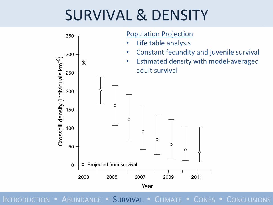
PopulaYon ProjecYon • Life table analysis • Constant fecundity and juvenile survival • EsYmated density with model-‐averaged
adult survival
Year
Cro
ssbi
ll de
nsity
(ind
ivid
uals
km−2
)
2003 2005 2007 2009 2011
0
50
100
150
200
250
300
350
SURVIVAL & DENSITY
INTRODUCTION � ABUNDANCE � SURVIVAL � CLIMATE � CONES � CONCLUSIONS
PopulaYon ProjecYon • Life table analysis • Constant fecundity and juvenile survival • EsYmated density with model-‐averaged
adult survival
Year
Cro
ssbi
ll de
nsity
(ind
ivid
uals
km−2
)
2003 2005 2007 2009 2011
0
50
100
150
200
250
300
350
●
●
●
●
●
●
●●
● Projected from survival

SURVIVAL & DENSITY
INTRODUCTION � ABUNDANCE � SURVIVAL � CLIMATE � CONES � CONCLUSIONS
●
●
●
●
●
●
●
●
Year
Cro
ssbi
ll de
nsity
(ind
ivid
uals
km−2
)
2003 2005 2007 2009 2011
0
50
100
150
200
250
300
350
●
●
●
●
●
●
●●
●
●
Point count estimateProjected from survival
PopulaYon ProjecYon • Life table analysis • Constant fecundity and juvenile survival • EsYmated density with model-‐averaged
adult survival

RESEARCH QUESTIONS
INTRODUCTION � ABUNDANCE � SURVIVAL � CLIMATE � CONES � CONCLUSIONS
• Is crossbill density conYnuing to decrease? • Do changes in survival account for the observed changes in density?
• Is crossbill survival related to climate? • Is cone producYvity decreasing?

CLIMATE COVARIATES
Variable Variable definiYon NHOT(X) number of hot (≥32°C), dry (<1 mm) days (unweighted and
weighted lags of 1-‐5 years) MSPR mean spring temperature (Mar – May) MSUM mean summer temperature (Jun – Aug) MANN mean annual temperature between captures (Jul – Jun) MNBY mean temperature in non-‐breeding year (Sep -‐ Mar) NCW number of cold (<5°C), wet (>1 mm) days
USGS NRCS SNOTEL data, 1989-‐current 2 km from banding site
INTRODUCTION � ABUNDANCE � SURVIVAL � CLIMATE � CONES � CONCLUSIONS

SURVIVAL & CLIMATE
Model ΔQAICc w R2 Φ(~MNBY) 0 0.59 0.59 Φ(~NHOT5) 1.66 0.26 0.51 Φ(~NHOT4) 4.16 0.07 0.40 Φ(~NHOT5.w33) 7.16 0.02 0.27 Φ(~MSPR) 7.56 0.01 0.25 Φ(~NHOT4.w33) 8.18 0.01 0.22
Modeled climate with survival Climate model = Φ(climate) 𝜌(year + sex)
INTRODUCTION � ABUNDANCE � SURVIVAL � CLIMATE � CONES � CONCLUSIONS

●
●
●
●
●
●
●
●
●
●
●
Mean temperature °C (September − March)
Appa
rent
adu
lt su
rviva
l
−1.0 −0.5 0.0 0.5 1.0 1.5 2.0
0.55
0.60
0.65
0.70
0.75
LOWER SURVIVAL WITH WARMER TEMPS
R2 = 0.55, P < 0.009
INTRODUCTION � ABUNDANCE � SURVIVAL � CLIMATE � CONES � CONCLUSIONS
●
●
●
●
●
●
●
●
●
●
●
Number of hot, dry days over previous five years
Appa
rent
adu
lt su
rviva
l
1.0 1.5 2.0 2.5 3.0 3.5
0.55
0.60
0.65
0.70
0.75
R2 = 0.52, P < 0.012
Number of hot, dry days over 5 previous years
Mean temperature (°C) (September – March)
Apparent su
rvival

RESEARCH QUESTIONS
INTRODUCTION � ABUNDANCE � SURVIVAL � CLIMATE � CONES � CONCLUSIONS
• Is crossbill density conYnuing to decrease? • Do changes in survival account for the observed changes in density?
• Is crossbill survivorship related to climate? • Is cone producYvity decreasing?

INTRODUCTION � ABUNDANCE � SURVIVAL � CLIMATE � CONES � CONCLUSIONS
CONE PRODUCTIVITY

INTRODUCTION � ABUNDANCE � SURVIVAL � CLIMATE � CONES � CONCLUSIONS
CONE PRODUCTIVITY
●
●
●
●
●
●
●
●
●
●
●
●
●
●
●
Year
Mea
n co
nes/
bran
ch/y
ear ±
1SE
1997 1999 2001 2003 2005 2007 2009 2011
0.6
0.8
1.0
1.2
1.4
1.6
1.8

1. PopulaYon is sYll declining 2. Changes in adult survival account for decline 3. Warmer temperatures decrease survival 4. Cone producYvity is likely not contribuYng to
populaYon decline
INTRODUCTION � ABUNDANCE � SURVIVAL � CLIMATE � CONES � CONCLUSIONS
SUMMARY
Supports main hypothesis

INTRODUCTION � ABUNDANCE � SURVIVAL � CLIMATE � CONES � CONCLUSIONS
MORE HOT DAYS
globalchange.gov
1961-‐1971 2080-‐2099

324 Climatic Change (2011) 105:313–328
Current 2020
2050 2080
a b
c d
Fig. 5 a–d Prediction of lodgepole pine distribution under current climate and the three future 30-year periods: 2020, 2050 and 2080
be almost absent from Oregon, Washington and Idaho. Even in British Columbiaand Alberta, the species’ range is likely to be reduced significantly (Fig. 5d). Thetotal area deemed suitable for the pine in the 2080 period is projected to be only15,000 km2, 17% of its current distribution. Of this area, 75% is currently modeled
INTRODUCTION � ABUNDANCE � SURVIVAL � CLIMATE � CONES � CONCLUSIONS
LODGEPOLE PINE DISTRIBUTION
Coops and Waring 2011, Clima;c Change
Current 2080

• Curb global warming
INTRODUCTION � ABUNDANCE � SURVIVAL � CLIMATE � CONES � CONCLUSIONS
MANAGEMENT ACTIONS PopulaYon projecYon using demographic data from 2001-‐2007
0 50 100 150 200
01000
2000
3000
4000
Year
Mean c
rossbill abundance
Mean of 2000 simulaYons
Mean Crossbill Abu
ndance
Years
ExYnct in 50 years

Reciprocal Selection between Crossbills and Pine 183
Figure 1: Distribution of lodgepole pine (black), locations of study sites, and representative red crossbills (Loxia curvirostra complex) and cones inthe Rocky Mountains (lower right), in the Cypress Hills (upper right), and in the South Hills and Albion Mountains (lower left; modified fromBenkman 1999). The crossbills and cones are drawn to relative scale. Red squirrels (Tamiasciurus hudsonicus) are found throughout the range oflodgepole pine except in some isolated mountains, including the South Hills (SH), Albion Mountains (AM), and Little Rocky Mountains (LR).Tamiasciurus were absent from the Cypress Hills (CH) until they were introduced in 1950.
in the strength and outcome of interactions might arise(Benkman 1999; Benkman et al. 2001). Where Tamiasciu-rus are present, they act as the dominant seed predatorand drive lodgepole pine cone evolution. These areas rep-resent a coevolutionary hot spot for Tamiasciurus and pinebut a coevolutionary cold spot for crossbills. Here cross-bills adapt to cones (fig. 1) whose evolution is largely theresult of selection by Tamiasciurus. Where Tamiasciurusare absent, however, crossbills act as the primary seed pred-ators, and they drive the evolution of lodgepole pine conetraits. In these areas, crossbills exhibit reciprocal adapta-tions implicating coevolution as an active process, making
such areas coevolutionary hot spots for crossbills (fig. 1).The result is divergent selection between populations ofcrossbills and pine in hot spots and cold spots.
This scenario is based on behavioral, morphological,genetical, and paleobotanical evidence that indicate rep-licated reciprocal adaptation and coevolution betweencrossbills and lodgepole pine east and west of the RockyMountains in the past 10,000 yr (fig. 1; Benkman 1999;Benkman et al. 2001). However, direct measures of naturalselection on lodgepole pine by crossbills and reciprocalselection by lodgepole pine on crossbills are lacking. Earlierstudies (Benkman 1999; Benkman et al. 2001) inferred
South Hills Type 5
• Curb global warming • Assisted migraYon
INTRODUCTION � ABUNDANCE � SURVIVAL � CLIMATE � CONES � CONCLUSIONS
MANAGEMENT ACTIONS

• Curb global warming • Assisted migraYon • Plant more lodgepole
INTRODUCTION � ABUNDANCE � SURVIVAL � CLIMATE � CONES � CONCLUSIONS
MANAGEMENT ACTIONS

ACKNOWLEDGEMENTS
Field Assistants • Bayasa Amgalen • Jeff Garcia • Michael Hague • Don Jones • Garrey MacDonald • James Maley • Carolyn Miller • Daniel Schlaepfer • Michael Woodruff • Charlie Wright
Funding • US EPA STAR • American Ornithologists’ Union • Berry Biodiversity Center • Program in Ecology • WYGISC GITA • Wyoming Chapter of The Wildlife Society • Zoology and Physiology Department
Commiyee • Craig Benkman • Merav Ben-‐David • Daniel Tinker
Photo Credits • Gary Dewaghe • Roger Garber • Nasim Mansurov • Nick Neely • Dennis Paulson • Lloyd Spitalnik • USFWS


MARK-‐RECAPTURE STUDY
INTRODUCTION � ABUNDANCE � SURVIVAL � CLIMATE � CONES � CONCLUSIONS