A Beginner’s Guideto

MATLAB*

Christos Xenophontos

Department of Mathematics & Computer Science

Clarkson University

Fall 1999

* Technical Report 98-02, Dept of Math. & Comp Sci., Clarkson University. MATLAB is a registeredtrademark of The MathWorks Inc.

2

TABLE OF CONTENTS

1. Introduction Page

1.1 MATLAB at Clarkson University 31.2 How to read this tutorial 4

2. MATLAB Basics

2.1 The basic features 42.2 Vectors and matrices 72.3 Built-in functions 132.4 Plotting 22

3. Programming in MATLAB

3.1 M-files : Scripts and functions 273.2 Loops 283.3 If statement 33

4. Additional Topics

4.1 Polynomials in MATLAB 364.2 Numerical Methods 38

5. Closing Remarks and References

References 43

3

1. INTRODUCTION

MATLAB, which stands for MATrix LABoratory, is a state-of-the-art mathematicalsoftware package, that is used extensively in both academia and industry. It is aninteractive program for numerical computation and data visualization, that along with itsprogramming capabilities provides a very useful tool for almost all areas of science andengineering. Unlike other mathematical packages, such as MAPLE or MATHEMATICA,MATLAB cannot perform symbolic manipulations without the use of additionalToolboxes. It remains however, one of the leading software packages for numericalcomputation.

As you might guess from its name, MATLAB deals mainly with matrices. A scalar is a 1-by-1 matrix and a row vector of length say 5, is a 1-by-5 matrix. We will elaborate moreon these and other features of MATLAB in the sections that follow. One of the manyadvantages of MATLAB is the natural notation used. It looks a lot like the notation thatyou encounter in a linear algebra course. This makes the use of the program especiallyeasy and it is what makes MATLAB a natural choice for numerical computations.

The purpose of this tutorial is to familiarize the beginner to MATLAB, by introducing thebasic features and commands of the program. It is in no way a complete reference and thereader is encouraged to further enhance his or her knowledge of MATLAB by readingsome of the suggested references at the end of this guide.

1.1 MATLAB at Clarkson University

MATLAB is available at Clarkson University both on the UNIX and the PC networks. Inaddition, if you are enrolled in a course that requires the use of MATLAB, you may obtainyour own time-locked copy for installation on your personal computer by simply visitingthe ERC and asking for the MATLAB CD.

It is a good idea to create a working directory where you will store your MATLAB files.On a UNIX machine, you may do so by using the mkdir directory_name command andyou may switch to that directory with the cd directory_name command. Once in theworking directory you may start MATLAB. If using a PC, first create the directory (usingthe command mkdir directory_name at the DOS prompt) and then start the program asdescribed below. Once you have MATLAB running, you may switch to the workingdirectory using the cd directory_name command within MATLAB.

To start the program on a UNIX machine, just type matlab at the prompt of a commandshell. You will then see the MATLAB prompt, which is two greater signs (»), and youwill be ready to type in your commands.

4

On a networked PC, such as those found in SC 334 or 338, you can start the program asfollows. Click on the Start button on the lower left corner of your desktop. This willproduce a menu in which you should choose (by clicking) the option Programs. Onemore menu will appear, that includes MATLAB as one of the available programs.Clicking on the MATLAB button will start the program in the form of a new window.The prompt (») will then appear and … off you go.

1.2 How to read this tutorial

In the sections that follow, the MATLAB prompt (») will be used to indicate where thecommands are entered. Anything you see after this prompt denotes user input (i.e. acommand) followed by a carriage return. Often, input is followed by output so unlessotherwise specified the line(s) that follow a command will denote output (i.e. MATLAB’sresponse to what you typed in). MATLAB is case-sensitive, which means that a + B isnot the same as a + b. Different fonts, like the ones you just witnessed, will also beused to simulate the interactive session. This can be seen in the example below :

e.g. MATLAB can work as a calculator. If we ask MATLAB to add two numbers, weget the answer we expected.

» 3 + 4

ans = 7

As we will see, MATLAB is much more than a “fancy” calculator. In order to get themost out this tutorial you are strongly encouraged to try all the commands introduced ineach section and work on all the recommended exercises. This usually works best if afterreading this guide once, you read it again (and possibly again and again) in front of acomputer.

2. MATLAB BASICS

2.1 The basic features

Let us start with something simple, like defining a row vector with components thenumbers 1, 2, 3, 4, 5 and assigning it a variable name, say x.

» x=[1 2 3 4 5]

x = 1 2 3 4 5

Note that we used the equal sign for assigning the variable name x to the vector, bracketsto enclose its entries and spaces to separate them. (Just like you would using the linear

5

algebra notation). We could have used commas ( , ) instead of spaces to separate theentries, or even a combination of the two. The use of either spaces or commas is essential!

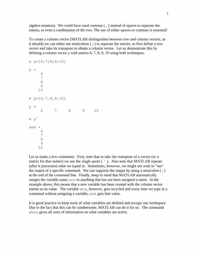
To create a column vector (MATLAB distinguishes between row and column vectors, asit should) we can either use semicolons ( ; ) to separate the entries, or first define a rowvector and take its transpose to obtain a column vector. Let us demonstrate this bydefining a column vector y with entries 6, 7, 8, 9, 10 using both techniques.

» y=[6;7;8;9;10]

y = 6 7 8 9 10

» y=[6,7,8,9,10]

y = 6 7 8 9 10

» y'

ans = 6 7 8 9 10

Let us make a few comments. First, note that to take the transpose of a vector (or amatrix for that matter) we use the single quote ( ' ). Also note that MATLAB repeats(after it processes) what we typed in. Sometimes, however, we might not wish to “see”the output of a specific command. We can suppress the output by using a semicolon ( ; )at the end of the command line. Finally, keep in mind that MATLAB automaticallyassigns the variable name ans to anything that has not been assigned a name. In theexample above, this means that a new variable has been created with the column vectorentries as its value. The variable ans, however, gets recycled and every time we type in acommand without assigning a variable, ans gets that value.

It is good practice to keep track of what variables are defined and occupy our workspace.Due to the fact that this can be cumbersome, MATLAB can do it for us. The commandwhos gives all sorts of information on what variables are active.

6

» whos

Name Size Elements Bytes Density Complex

ans 5 by 1 5 40 Full Nox 1 by 5 5 40 Full Noy 1 by 5 5 40 Full No

Grand total is 15 elements using 120 bytes

A similar command, called who , only provides the names of the variables that are active.

» who

Your variables are:

ans x y

If we no longer need a particular variable we can “delete” it from the memory using thecommand clear variable_name. Let us clear the variable ans and check thatwe indeed did so.

» clear ans» who

Your variables are:

x y

The command clear used by itself, “deletes” all the variables from the memory. Becareful, as this is not reversible and you do not have a second chance to change your mind.

You may exit the program using the quit command. When doing so, all variables arelost. However, invoking the command save filename before exiting, causes allvariables to be written to a binary file called filename.mat. When we start MATLABagain, we may retrieve the information in this file with the command load filename.We can also create an ascii (text) file containing the entire MATLAB session if we use thecommand diary filename at the beginning and at the end of our session. This willcreate a text file called filename (with no extension) that can be edited with any texteditor, printed out etc. This file will include everything we typed into MATLAB duringthe session (including error messages but excluding plots). We could also use thecommand save filename at the end of our session to create the binary file describedabove as well as the text file that includes our work.

One last command to mention before we start learning some more interesting things aboutMATLAB, is the help command. This provides on line help for any existing MATLABcommand. Let us try this command on the command who.

7

» help who

WHO List current variables. WHO lists the variables in the current workspace. WHOS lists more information about each variable. WHO GLOBAL and WHOS GLOBAL list the variables in the

global workspace.

Try using the command help on itself!

If you are using a PC, help is also available from the Window Menus. Sometimes, it iseasier to look up a command from the list provided there, instead of using the commandline help.

2.2 Vectors and matrices

We have already seen how to define a vector and assign a variable name to it. Often it isuseful to define vectors (and matrices) that contain equally spaced entries. This can bedone by specifying the first entry, an increment, and the last entry. MATLAB willautomatically figure out how many entries you need and their values. For example, tocreate a vector whose entries are 0, 1, 2, 3, …, 7, 8, you can type

» u = [0:8]

u = 0 1 2 3 4 5 6 7 8

Here we specified the first entry 0, and the last entry 8, separated by a colon ( : ).MATLAB automatically filled-in the (omitted) entries using the (default) increment 1.You could also specify an increment as is done in the next example.

To obtain a vector whose entries are 0, 2, 4, 6, and 8, you can type in the following line:

» v = [0:2:8]

v = 0 2 4 6 8

Here we specified the first entry 0, the increment value 2, and the last entry 8. The twocolons ( : ) “tell” MATLAB to fill in the (omitted) entries using the specified incrementvalue.

MATLAB will allow you to look at specific parts of the vector. If you want, for example,to only look at the first 3 entries in the vector v, you can use the same notation you usedto create the vector :

8

» v(1:3)

ans = 0 2 4

Note that we used parentheses, instead of brackets, to refer to the entries of the vector.Since we omitted the increment value, MATLAB automatically assumes that theincrement is 1. The following command lists the first 4 entries of the vector v, using theincrement value 2 :

» v(1:2:4)

ans = 0 4

Defining a matrix is similar to defining a vector. To define a matrix A, you can treat it likea column of row vectors. That is, you enter each row of the matrix as a row vector(remember to separate the entries either by commas or spaces) and you separate the rowsby semicolons ( ; ).

» A = [1 2 3; 3 4 5; 6 7 8]

A = 1 2 3 3 4 5 6 7 8

We can avoid separating each row with a semicolon if we use a carriage return instead. Inother words, we could have defined A as follows

» A=[1 2 33 4 56 7 8]

A = 1 2 3 3 4 5 6 7 8

which is perhaps closer to the way we would have defined A by hand using the linearalgebra notation.

You can refer to a particular entry in a matrix by using parentheses. For example, thenumber 5 lies in the 2nd row, 3rd column of A, thus

» A(2,3)

9

ans = 5

The order of rows and columns follows the convention adopted in the linear algebranotation. This means that A(2,3) refers to the number 5 in the above example andA(3,2) refers to the number 7, which is in the 3rd row, 2nd column.

Note MATLAB’s response when we ask for the entry in the 4th row, 1st column.

» A(4,1)??? Index exceeds matrix dimensions.

As expected, we get an error message. Since A is a 3-by-3 matrix, there is no 4th row andMATLAB realizes that. The error messages that we get from MATLAB can be quiteinformative when trying to find out what went wrong. In this case MATLAB told usexactly what the problem was.

We can “extract” submatrices using a similar notation as above. For example to obtain thesubmatrix that consists of the first two rows and last two columns of A we type

» A(1:2,2:3)

ans = 2 3 4 5

We could even extract an entire row or column of a matrix, using the colon ( : ) asfollows. Suppose we want to get the 2nd column of A. We basically want the elements[A(1,2) A(2,2) A(3,2)]. We type

» A(:,2)

ans = 2 4 7

where the colon was used to tell MATLAB that all the rows are to be used. The same canbe done when we want to extract an entire row, say the 3rd one.

» A(3,:)

ans = 6 7 8

Define now another matrix B, and two vectors s and t that will be used in what follows.

10

» B = [-1 3 10-9 5 250 14 2]

B = -1 3 10 -9 5 25 0 14 2

» s=[-1 8 5]

s = -1 8 5

» t=[7;0;11]

t = 7 0 11

The real power of MATLAB is the ease in which you can manipulate your vectors andmatrices. For example, to subtract 1 from every entry in the matrix A we type

» A-1

ans = 0 1 2 2 3 4 5 6 7

It is just as easy to add (or subtract) two compatible matrices (i.e. matrices of the samesize).

» A+B

ans = 0 5 13 -6 9 30 6 21 10

The same is true for vectors.

» s-t??? Error using ==> -Matrix dimensions must agree.

11

This error was expected, since s has size 1-by-3 and t has size 3-by-1. We will not get anerror if we type

» s-t'

ans = -8 8 -6since by taking the transpose of t we make the two vectors compatible.

We must be equally careful when using multiplication.

» B*s??? Error using ==> *Inner matrix dimensions must agree.

» B*t

ans = 103 212 22

Another important operation that MATLAB can perform with ease is “matrix division”. IfM is an invertible square matrix and b is a compatible vector then

x = M\b is the solution of M x = b andx = b/M is the solution of x M = b.

Let us illustrate the first of the two operations above with M = B and b = t.

» x=B\t

x = 2.4307 0.6801 0.7390

x is the solution of B x = t as can be seen in the multiplication below.

» B*x

ans = 7.0000 0.0000 11.0000

Since x does not consist of integers, it is worth while mentioning here the commandformat long. MATLAB only displays four digits beyond the decimal point of a real

12

number unless we use the command format long, which tells MATLAB to displaymore digits.

» format long

» x

x = 2.43071593533487 0.68013856812933 0.73903002309469

On a PC, the command format long can also be used through the Window Menus.

There are many times when we want to perform an operation to every entry in a vector ormatrix. MATLAB will allow us to do this with “element-wise” operations.

For example, suppose you want to multiply each entry in the vector s with itself. In otherwords, suppose you want to obtain the vector s2 = [s(1)*s(1), s(2)*s(2), s(3)*s(3)].

The command s*s will not work due to incompatibility. What is needed here is to tellMATLAB to perform the multiplication element-wise. This is done with the symbols".*". In fact, you can put a period in front of most operators to tell MATLAB that youwant the operation to take place on each entry of the vector (or matrix).

» s*s??? Error using ==> *Inner matrix dimensions must agree.

» s.*s

ans = 1 64 25

The symbol " .^ " can also be used since we are after all raising s to a power. (The periodis needed here as well.)

» s.^2

ans = 1 64 25

The table below summarizes the operators that are available in MATLAB.

+ addition- subtraction* multiplication

13

^ power' transpose\ left division/ right division

Remember that the multiplication, power and division operators can be used inconjunction with a period to specify an element-wise operation.

Exercises

Create a diary session called sec2_2 in which you should complete the followingexercises.

Define

[ ]A b a=

=

−

= − −

2 9 0 0

0 4 1 4

7 5 5 1

7 8 7 4

1

6

0

9

3 2 4 5, ,

1. Calculate the following (when defined)

(a) A ⋅ b (b) a + 4 (c) b ⋅ a (d) a ⋅ bT (e) A ⋅ aT

2. Explain any differences between the answers that MATLAB gives when you type inA*A , A^2 and A.^2.

3. What is the command that isolates the submatrix that consists of the 2nd to 3rd rows ofthe matrix A?

4. Solve the linear system A x = b for x. Check your answer by multiplication.

Edit your text file to delete any errors (or typos) and hand in a readable printout.

2.3 Built-in functions

There are numerous built-in functions (i.e. commands) in MATLAB. We will mention afew of them in this section by separating them into categories.

Scalar Functions

Certain MATLAB functions are essentially used on scalars, but operate element-wisewhen applied to a matrix (or vector). They are summarized in the table below.

14

sin trigonometric sinecos trigonometric cosinetan trigonometric tangentasin trigonometric inverse sine (arcsine)acos trigonometric inverse cosine (arccosine)atan trigonometric inverse tangent (arctangent)exp exponentiallog natural logarithmabs absolute valuesqrt square rootrem remainderround round towards nearest integerfloor round towards negative infinityceil round towards positive infinity

Even though we will illustrate some of the above commands below, it is stronglyrecommended to get help on all of them to find out exactly how they are used.

The trigonometric functions take as input radians. Since MATLAB uses pi for thenumber π=3.1415…

» sin(pi/2)

ans = 1

» cos(pi/2)

ans = 6.1230e-017

The sine of π/2 is indeed 1 but we expected the cosine of π/2 to be 0. Well, rememberthat MATLAB is a numerical package and the answer we got (in scientific notation) isvery close to 0 ( 6.1230e-017 = 6.1230×10 -17 ≈ 0).

Since the exp and log commands are straight forward to use, let us illustrate some of theother commands. The rem command gives the remainder of a division. So the remainderof 12 divided by 4 is zero

» rem(12,4)

ans = 0

and the remainder of 12 divided by 5 is 2.

15

» rem(12,5)

ans = 2

The floor, ceil and round commands are illustrated below.

» floor(1.4)ans = 1

» ceil(1.4)

ans = 2

» round(1.4)

ans = 1

Keep in mind that all of the above commands can be used on vectors with the operationtaking place element-wise. For example, if x = [0, 0.1, 0.2, . . ., 0.9, 1], theny = exp(x) will produce another vector y , of the same length as x, whose entries are givenby y = [e0, e0.1, e0.2, . . ., e1].

» x=[0:0.1:1]

x =

Columns 1 through 7

0 0.1000 0.2000 0.3000 0.4000 0.5000 0.6000

Columns 8 through 11

0.7000 0.8000 0.9000 1.0000

» y=exp(x)

y =

Columns 1 through 7

1.0000 1.1052 1.2214 1.3499 1.4918 1.6487 1.8221

Columns 8 through 11

2.0138 2.2255 2.4596 2.7183

16

This is extremely useful when plotting data. See Section 2.4 ahead for more details onplotting.

Also, note that MATLAB displayed the results as 1-by-11 matrices (i.e. row vectors oflength 11). Since there was not enough space on one line for the vectors to be displayed,MATLAB reports the column numbers.

Vector Functions

Other MATLAB functions operate essentially on vectors returning a scalar value. Someof these functions are given in the table below.

max largest componentmin smallest componentlength length of a vectorsort sort in ascending ordersum sum of elementsprod product of elementsmedian median valuemean mean valuestd standard deviation

Once again, it is strongly suggested to get help on all the above commands. Some areillustrated below.

Let z be the following row vector.

» z=[0.9347,0.3835,0.5194,0.8310]

z = 0.9347 0.3835 0.5194 0.8310

Then

» max(z)

ans = 0.9347

» min(z)

ans = 0.3835

» sort(z)

17

ans = 0.3835 0.5194 0.8310 0.9347

» sum(z)

ans = 2.6686

» mean(z)ans = 0.6671

The above vector function can also be applied to a matrix. In this case, they act in acolumn-by-column fashion to produce a row vector containing the results of theirapplication to each column. The example below illustrates the use of the above (vector)commands on matrices.

Suppose we wanted to find the maximum element in the following matrix.

» M = [0.7012,0.2625,0.32820.9103,0.0475,0.63260.7622,0.7361,0.7564]

M= 0.7012 0.2625 0.3282 0.9103 0.0475 0.6326 0.7622 0.7361 0.7564

If we used the max command on M, we will get the row in which the maximum elementlies (remember the vector functions act on matrices in a column-by-column fashion).

» max(M)

ans = 0.9103 0.7361 0.7564

To isolate the largest element, we must use the max command on the above row vector.Taking advantage of the fact that MATLAB assigns the variable name ans to the answerwe obtained, we can simply type

» max(ans)

ans = 0.9103

The two steps above can be combined into one in the following.

18

» max(max(M))

ans = 0.9103

Combining MATLAB commands can be very useful when programming complexalgorithms where we do not wish to see or access intermediate results. More on this, andother programming features of MATLAB in Section 3 ahead.

Matrix Functions

Much of MATLAB’s power comes from its matrix functions. These can be furtherseparated into two sub-categories. The first one consists of convenient matrix buildingfunctions, some of which are given in the table below.

eye identity matrixzeros matrix of zerosones matrix of onesdiag extract diagonal of a matrix or create diagonal

matricestriu upper triangular part of a matrixtril lower triangular part of a matrixrand randomly generated matrix

Make sure you ask for help on all the above commands.

To create the identity matrix of size 4 (i.e. a square 4-by-4 matrix with ones on the maindiagonal and zeros everywhere else) we use the command eye.

» eye(4,4)

ans = 1 0 0 0 0 1 0 0 0 0 1 0 0 0 0 1

The numbers in parenthesis indicates the size of the matrix. When creating squarematrices, we can specify only one input referring to size of the matrix. For example, wecould have obtained the above identity matrix by simply typing eye(4). The same is truefor the matrix building functions below.

Similarly, the command zeros creates a matrix of zeros and the command ones createsa matrix of ones.

» zeros(2,3)

19

ans = 0 0 0 0 0 0

» ones(2)

ans = 1 1 1 1We can create a randomly generated matrix using the rand command. (The entries willbe uniformly distributed between 0 and 1.)

» C=rand(5,4)

C = 0.2190 0.3835 0.5297 0.4175 0.0470 0.5194 0.6711 0.6868 0.6789 0.8310 0.0077 0.5890 0.6793 0.0346 0.3834 0.9304 0.9347 0.0535 0.0668 0.8462

The commands triu and tril, extract the upper and lower part of a matrix,respectively. Let us try them on the matrix C defined above.

» triu(C)

ans = 0.2190 0.3835 0.5297 0.4175 0 0.5194 0.6711 0.6868 0 0 0.0077 0.5890 0 0 0 0.9304 0 0 0 0

» tril(C)

ans = 0.2190 0 0 0 0.0470 0.5194 0 0 0.6789 0.8310 0.0077 0 0.6793 0.0346 0.3834 0.9304 0.9347 0.0535 0.0668 0.8462

Once the extraction took place, the “empty” positions in the new matrices areautomatically filled with zeros.

As mentioned earlier, the command diag has two uses. The first use is to extract adiagonal of a matrix, e.g. the main diagonal. Suppose D is the matrix given below. Then,diag(D) produces a column vector, whose components are the elements of D that lieon its main diagonal.

20

» D = [0.9092 0.5045 0.98660.0606 0.5163 0.49400.9047,0.3190,0.2661];

» diag(D)

ans = 0.9092 0.5163 0.2661

The second use is to create diagonal matrices. For example,

» diag([0.9092;0.5163;0.2661])

ans = 0.9092 0 0 0 0.5163 0 0 0 0.2661

creates a diagonal matrix whose non-zero entries are specified by the vector given asinput.

This command is not restricted to the main diagonal of a matrix; it works on off diagonalsas well. See help diag for more information.

Let us now summarize some of the commands in the second sub-category of matrixfunctions.

size size of a matrixdet determinant of a square matrixinv inverse of a matrixrank rank of a matrixrref reduced row echelon formeig eigenvalues and eigenvectorspoly characteristic polynomialnorm norm of matrix (1-norm, 2-norm, ∞ -norm)cond condition number in the 2-normlu LU factorizationqr QR factorizationchol Cholesky decompositionsvd singular value decomposition

Don’t forget to get help on the above commands. To illustrate a few of them, define thefollowing matrix.

21

» A=[9,7,0;0,8,6;7,1,-6]

A = 9 7 0 0 8 6 7 1 -6

» size(A)

ans = 3 3

» det(A)

ans = -192

Since the determinant is not zero, the matrix is invertible.

» inv(A)

ans = 0.2812 -0.2187 -0.2187 -0.2187 0.2812 0.2812 0.2917 -0.2083 -0.3750

We can check our result by verifying that AA-1 = I and A-1A = I .

» A*inv(A)

ans = 1.0000 0.0000 0.0000 0.0000 1.0000 0.0000 0.0000 0.0000 1.0000

» inv(A)*A

ans = 1.0000 0.0000 0 0.0000 1.0000 0 0.0000 0 1.0000

Let us comment on why MATLAB uses both 0’s and 0.0000’s in the answer above.Recall that we are dealing with a numerical package that uses numerical algorithms toperform the operations we ask for. Hence, the use of floating point (vs. exact) arithmeticcauses the “discrepancy” in the results. From a practical point of view, 0 and 0.0000 arethe same.

The eigenvalues and eigenvectors of A (i.e. the numbers λ and vectors x that solveAx = λx ) can be obtained through the eig command.

22

» eig(A)

ans = 12.6462 3.1594 -4.8055produces a column vector with the eigenvalues and

» [X,D]=eig(A)

X = -0.8351 -0.6821 0.2103 -0.4350 0.5691 -0.4148 -0.3368 -0.4592 0.8853

D = 12.6462 0 0 0 3.1594 0 0 0 -4.8055

produces a diagonal matrix D with the eigenvalues on the main diagonal, and a full matrixX whose columns are the corresponding eigenvectors.

Exercises

Create a diary session called sec2_3 in which you should complete the followingexercises using MATLAB commands. When applicable, use the matrix A and the vectorsb, a that were defined in the previous section’s exercises.1. Construct a randomly generated 2-by-2 matrix of positive integers.

2. Find the maximum and minimum elements in the matrix A.

3. Sort the values of the vector b.

4. (a) Find the eigenvalues and eigenvectors of the matrix B = A-1. Store the eigenvaluesin a column vector you should name lambda.(b) With I the 4-by-4 identity matrix, calculate the determinant of the matrixB - lambdaj I , for j = 1, 2, 3, 4. (Note : lambda1 is the first eigenvalue, lambda2 isthe second eigenvalue etc.)

2.4 Plotting

We end our discussion on the Basic Features of MATLAB by introducing the commandsfor data visualization (i.e. plotting). By typing help plot you can see the various

23

capabilities of this main command for two-dimensional plotting, some of which will beillustrated below.

If x and y are two vectors of the same length then plot(x,y) plots x versus y.

For example, to obtain the graph of y = cos(x) from - π to π, we can first define the vectorx with components equally spaced numbers between - π and π, with increment 0.01.

» x=-pi:0.01:pi;

We placed a semicolon at the end of the input line to avoid seeing the (long) output.Note that the smallest the increment, the “smoother” the curve will be.

Next, we define the vector y

» y=cos(x);

(using a semicolon again) and we ask for the plot

» plot(x,y)

At this point a new window will appear on our desktop in which the graph (as seen below)will appear.

-4 -3 -2 -1 0 1 2 3 4-1

-0.8

-0.6

-0.4

-0.2

0

0.2

0.4

0.6

0.8

1

It is good practice to label the axis on a graph and if applicable indicate what each axisrepresents. This can be done with the xlabel and ylabel commands.

» xlabel('x')» ylabel('y=cos(x)')

24

Inside parentheses, and enclosed within single quotes, we type the text that we wish to bedisplayed along the x and y axis, respectively.

We could even put a title on top using

» title('Graph of cosine from -pi to pi')as long as we remember to enclose the text in parentheses within single quotes.

These commands can be invoked even after the plot window has been opened andMATLAB will make all the necessary adjustments to the display.

-4 -3 -2 -1 0 1 2 3 4-1

-0.8

-0.6

-0.4

-0.2

0

0.2

0.4

0.6

0.8

1

x

y=co

s(x)

Graph of cosine from -pi to pi

Various line types, plot symbols and colors can be used. If these are not specified (as inthe case above) MATLAB will assign (and cycle through) the default ones as given in thetable below.

y yellow . point m magenta o circle c cyan x x-mark r red + plus g green - solid b blue * star w white : dotted k black -. dashdot -- dashed

So, to obtain the same graph but in green, we type

» plot(x,y,’g’)

where the third argument indicating the color, appears within single quotes. We could geta dashed line instead of a solid one by typing

25

» plot(x,y,’--’)

or even a combination of line type and color, say a blue dotted line by typing

» plot(x,y,’b:’)

Multiple curves can appear on the same graph. If for example we define another vector

» z=sin(x);

we can get both graphs on the same axis, distinguished by their line type, using

» plot(x,y,'--',x,z,':')

The resulting graph can be seen below, with the dashed line representing y = cos(x) andthe dotted line representing z = sin(x).

-4 -3 -2 -1 0 1 2 3 4-1

-0.8

-0.6

-0.4

-0.2

0

0.2

0.4

0.6

0.8

1

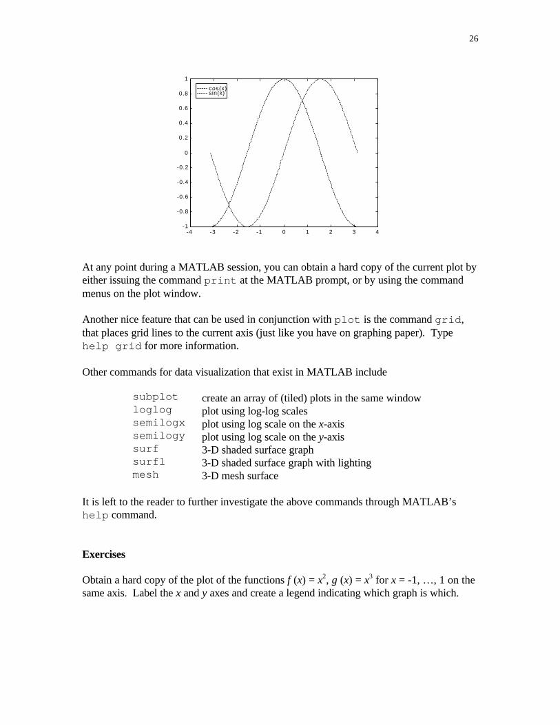
When multiple curves appear on the same axis, it is a good idea to create a legend to labeland distinguish them. The command legend does exactly this.

» legend('cos(x)','sin(x)')

The text that appears within single quotes as input to this command, represents the legendlabels. We must be consistent with the ordering of the two curves, so since in the plotcommand we asked for cosine to be plotted before sine, we must do the same here.

26

cos(x)sin(x)

-4 -3 -2 -1 0 1 2 3 4-1

-0.8

-0.6

-0.4

-0.2

0

0.2

0.4

0.6

0.8

1

At any point during a MATLAB session, you can obtain a hard copy of the current plot byeither issuing the command print at the MATLAB prompt, or by using the commandmenus on the plot window.

Another nice feature that can be used in conjunction with plot is the command grid,that places grid lines to the current axis (just like you have on graphing paper). Typehelp grid for more information.

Other commands for data visualization that exist in MATLAB include

subplot create an array of (tiled) plots in the same windowloglog plot using log-log scalessemilogx plot using log scale on the x-axissemilogy plot using log scale on the y-axissurf 3-D shaded surface graphsurfl 3-D shaded surface graph with lightingmesh 3-D mesh surface

It is left to the reader to further investigate the above commands through MATLAB’shelp command.

Exercises

Obtain a hard copy of the plot of the functions f (x) = x2, g (x) = x3 for x = -1, …, 1 on thesame axis. Label the x and y axes and create a legend indicating which graph is which.

27

3. PROGRAMMING IN MATLAB

3.1 M-files : Scripts and functions

To take advantage of MATLAB’s full capabilities, we need to know how to constructlong (and sometimes complex) sequences of statements. This can be done by writing thecommands in a file and calling it from within MATLAB. Such files are called “m-files”because they must have the filename extension “.m”. This extension is required in orderfor these files to be interpreted by MATLAB.

There are two types of m-files : script files and function files. Script files contain asequence of usual MATLAB commands, that are executed (in order) once the script iscalled within MATLAB. For example, if such a file has the name compute.m , thentyping the command compute at the MATLAB prompt will cause the statements in thatfile to be executed. Script files can be very useful when entering data into a matrix.

Function files, on the other hand, play the role of user defined commands that often haveinput and output. You can create your own commands for specific problems this way,which will have the same status as other MATLAB commands. Let us give a simpleexample. The text below is saved in a file called log3.m and it is used to calculate thebase 3 logarithm of a positive number. The text file can be created in a variety of ways,for example using the built-in MATLAB editor through the command edit(that isavailable with versions 5 and above), or your favorite (external) text editor (e.g. vi inUNIX or notepad in WINDOWS). You must make sure that the filename has theextension “.m” !

function [a] = log3(x)

% [a] = log3(x) - Calculates the base 3 logarithm of x.

a = log(abs(x))./log(3);

% End of function

Using this function within MATLAB to compute log 3(5), we get

» log3(5)

ans = 1.4650

Let us explain a few things related to the syntax of a function file. Every MATLABfunction begins with a header, which consists of the following :

(a) the word function,(b) the output(s) in brackets, (the variable a in the above example)(c) the equal sign,

28

(d) the name of the function, which must match the function filename (log3 in the aboveexample) and

(e) the input(s) (the variable x in the above example).

Any statement that appears after a “%” sign on a line is ignored by MATLAB and plays therole of comments in the subroutine. Comments are essential when writing long functionsor programs, for clarity. In addition, the first set of comments after the header in afunction serve as on-line help. For example, see what happens when we type

» help log3

[a] = log3(x) - Calculates the base 3 logarithm of x.

MATLAB gave us as “help” on the function we defined, the text that we included after theheader in the file.

Finally, the algorithm used to calculate the base 3 logarithm of a given number, is based onthe formula

log 3(x) = ln(|x|) / ln(3).

Since the logarithm of a negative number is undefined, we use the absolute value for“safety”. Also, note that we have allowed for a vector to be passed as input, by usingelement-wise division in the formula.

During a MATLAB session, we may call a function just like we did in the above example,provided the file is saved in the current (working) directory. This is the reason why in thebeginning of this guide we suggested that you should create a working directory and startMATLAB from there.

It should be noted that both types of m-files can reference other m-files, includingthemselves in a recursive way.

Exercises

Write a script m-file called rand_int.m that once called within MATLAB gives arandom integer.

3.2 Loops

We will now cover some commands for creating loops, that are not only used in writingm-files, but in regular MATLAB sessions as well. The examples that we will give willinclude both situations. The two types of loops that we will discuss are “for” and “while”loops. Both loop structures in MATLAB start with a keyword such as for, or whileand they end with the word end.

29

The “for” loop allows us to repeat certain commands. If you want to repeat some actionin a predetermined way, you can use the “for” loop. The “for” loop will loop around somestatement, and you must tell MATLAB where to start and where to end.For example,

>> for j=1:4 j end

j = 1

j = 2

j = 3

j = 4

looped through the numbers 1, …, 4 and every time printed the current number.

Enclosed between the for and end, you can have multiple statements just like in theexample below. Here, we define the vector x = [1, 2, …, 10] and we calculatex2 = [12, 22, …, 102], which we name x2. The semicolon at the end of the inner statementin the loop suppresses the printing of unwanted intermediate results.

» x=1:10

x = 1 2 3 4 5 6 7 8 9 10

» for i=1:10 x2(i) = x(i)^2; end

» x2

x2 = 1 4 9 16 25 36 49 64 81 100

Even though for loops are convenient to use in certain cases, they are not always the mostefficient way to perform an operation. In the above example, we would have been betteroff using

» x2 = x.^2

30

x2 = 1 4 9 16 25 36 49 64 81 100

instead. There are occasions, however, where the “vectorized” notation of MATLABcannot help us perform the operations we want, and loops are needed despite the fact thatthey are not as efficient.

Nested loops can also be created. In the following example, we calculate the square of theentries in a matrix. (This again is not as efficient but it is used for illustration)

» A=[1,5,-3;2,4,0;-1,6,9]

A = 1 5 -3 2 4 0 -1 6 9

» for i=1:3 for j=1:3 A2(i,j) = A(i,j)^2; end end

» A2

A2 = 1 25 9 4 16 0 1 36 81

For a more realistic example, consider the m-file gaussel.m, which performs Gaussianelimination (and back substitution) to solve the square system A x = b.

function [x] = gaussel(A,b)

% [x] = gaussel(A,b)%% This subroutine will perform Gaussian elimination% and back substitution to solve the system Ax = b.%% INPUT : A - matrix for the left hand side.% b - vector for the right hand side%% OUTPUT : x - the solution vector.

N = max(size(A));

% Perform Gaussian Elimination

31

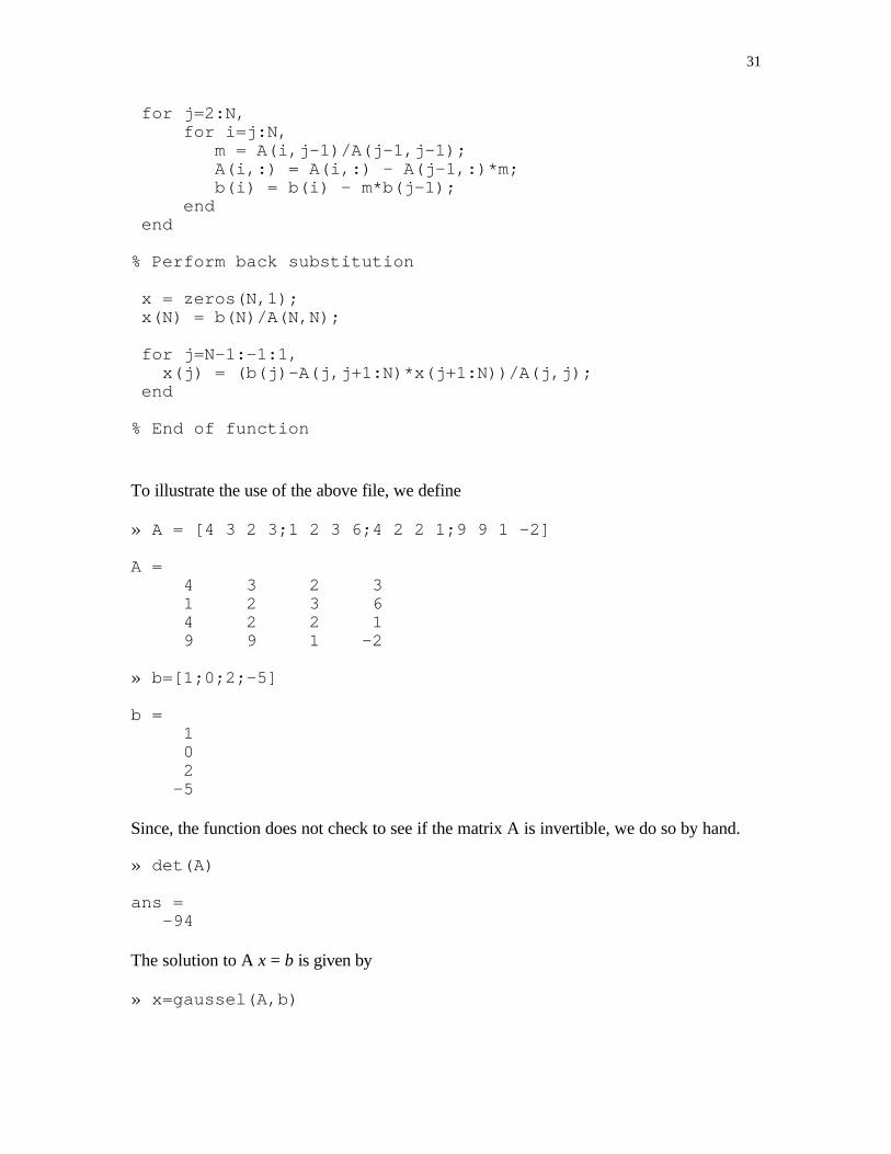
for j=2:N, for i=j:N, m = A(i,j-1)/A(j-1,j-1); A(i,:) = A(i,:) - A(j-1,:)*m; b(i) = b(i) - m*b(j-1); end end

% Perform back substitution

x = zeros(N,1); x(N) = b(N)/A(N,N);

for j=N-1:-1:1, x(j) = (b(j)-A(j,j+1:N)*x(j+1:N))/A(j,j); end

% End of function

To illustrate the use of the above file, we define

» A = [4 3 2 3;1 2 3 6;4 2 2 1;9 9 1 -2]

A = 4 3 2 3 1 2 3 6 4 2 2 1 9 9 1 -2

» b=[1;0;2;-5]

b = 1 0 2 -5

Since, the function does not check to see if the matrix A is invertible, we do so by hand.

» det(A)

ans = -94

The solution to A x = b is given by

» x=gaussel(A,b)

32

x = 1.2979 -1.7660 -0.0213 0.3830

Of course, a more efficient way to solve such a linear system would be through the built-inMATLAB solver. That is, we could have typed x = A\b to obtain the same answer.Try it!

The second type of loop is the “while” loop. The “while” loop repeats a sequence ofcommands as long as some condition is met. For example, given a number n, thefollowing m-file (exple.m) will display the smallest non-negative integer a such that2a ≥ n.

function [a] = exple(n)

% [a] = exple(n)%

a = 0;while 2^a < n a = a + 1;end

% End of function

» a=exple(4)

a = 2

The conditional statement in the “while” loop is what makes it differ from the “for” loop.In the above example we used the conditional statement

while 2^a < n

which meant that MATLAB would check to see if this condition is met, and if so proceedwith the statement that followed. Such conditional statements are also used in “if”statements that are discussed in the next section. To form a conditional statement we userelational operators. The following are available in MATLAB.

< less than> greater than<= less than or equal>= greater than or equal== equal~= not equal

33

Note that “=” is used in assignments and “= =” is used in relations. Relations may beconnected (or quantified) by the following logical operators.

& and| or~ not

Exercises

The n-by-n Hilbert matrix H, has as its entries Hi,j = 1/(i + j - 1), i,j = 1, 2, …, n. Create adouble “for loop” to generate the 5-by-5 Hilbert matrix and check your answer using thebuilt-in MATLAB command hilb.

3.3 If statement

There are times when you would like your algorithm/code to make a decision, and the “if”statement is the way to do it. The general syntax in MATLAB is as follows :

if relation statement(s)elseif relation % if applicable statement(s) % if applicableelse % if applicable statement(s) % if applicableend

The logical operators (&, |, ~) could also be used to create more complex relations.

Let us illustrate the “if” statement through a simple example. Suppose we would like todefine and plot the piecewise defined function

Fx if x

if x=

− < <≤ <

2 1 0 5

0 25 0 5 1

.

. .

This is done with the use of the “if” statement in MATLAB as follows. First we define the“domain” vector x from -1 to 1 with increment 0.01 to produce a smooth enough curve.

» x=-1:0.01:1;

Next, we loop through the values of x and for each one we create the correspondingfunction value F as a vector.

34

» for i=1:length(x) if x(i) < 0.5 F(i) = x(i)^2; else F(i) = 0.25; end end

Finally, we plot the two vectors.

» plot(x,F)

-1 -0.5 0 0.5 10

0.1

0.2

0.3

0.4

0.5

0.6

0.7

0.8

0.9

1

As a second example, we would like to write a subroutine that takes as input a squarematrix and returns its inverse (if it exists). The m-file below (chk_inv.m) will performthis task for us, and make use of the “if” statement. If the matrix is not square or if it doesnot have an inverse, the subroutine should print a message letting us know and it willterminate without computing anything. We will also make use of comments within the m-file to make it more readable.

function [Ainv] = chk_inv(A)

% [Ainv] = chk_inv(A)% Calculate the inverse of a matrix A% if it exists.

[m,n] = size(A); % compute the size of the matrix Aif m~=n % check if A is square disp('Matrix is not square.'); break % quit the functionelseif det(A)==0 % check if A is singular disp('Matrix is singular.'); break % quit the functionelse

35

Ainv = inv(A); % compute the inverseend

% End of function

Here is a sample run of the above program with a random 3-by-3 matrix.

» A=rand(3,3)

A = 0.0475 0.6326 0.3653 0.7361 0.7564 0.2470 0.3282 0.9910 0.9826

» chk_inv(A)

ans = -2.4101 1.2551 0.5806 3.1053 0.3544 -1.2437 -2.3270 -0.7767 2.0783

It is left to the reader to see what answers other input matrices will produce.

In the above m-file, we used two “new” commands : disp and break. As you couldimagine, break simply causes the current operation to stop (exit the program in thiscase). The command disp takes as input text enclosed within single quotes and displaysit on the screen. See help disp for more information of this and other text displayingcommands.

As a final example, let us write an m-file called fact.m that gives the factorial of apositive number n = 1⋅2⋅3⋅4 . . . (n - 1)⋅n, using the recursive formula n! = n (n - 1). Thisexample will not only illustrate the use of the “if” statement, but that of a recursivefunction as well.

function [N] = fact(n)

% [N] = fact(n)% Calculate n factorial

if (n = = 1) | (n = = 0) N = 1;else N = fact(n-1);end

% End of function

36

Exercises

1. Modify the m-file log3.m from Section 3.1, by removing the absolute value within thelogarithms (that was used for “safety”). Your function should now check to see if theinput is negative or zero, print out a message saying so, and then terminate. If the inputis positive then your function should proceed to calculate the logarithm base 3 of theinput.

2. Write a function m-file called div5.m that takes as input a real number and checks tosee if it is divisible by 5. An appropriate message indicating the result should be theoutput.

4. ADDITIONAL TOPICS

4.1 Polynomials in MATLAB

Even though MATLAB is a numerical package, it has capabilities for handlingpolynomials. In MATLAB, a polynomial is represented by a vector containing itscoefficients in descending order. For instance, the following polynomial

p(x) = x2 -3x + 5

is represented by the vector p = [1, -3, 5] and the polynomial

q(x) = x4 +7x2 - x

is represented by q = [1, 0, 7, -1,0] .

MATLAB can interpret any vector of length n + 1 as an nth order polynomial. Thus, ifyour polynomial is missing any coefficients, you must enter zeros in the appropriateplace(s) in the vector, as done above.

You can find the value of a polynomial using the polyval command. For example, tofind the value of the polynomial q above at x = -1, you type

» polyval(q,-1)

ans = 7

Finding the roots of a polynomial is as easy as entering the following command.

» roots(q)

37

ans = 0 0.0712 + 2.6486i 0.0712 - 2.6486i -0.1424

Note that MATLAB can handle complex numbers as well, with i=sqrt(-1). This isreflected in the four roots above, two of which are complex.

Suppose you want to multiply two polynomials together. Their product is found by takingthe convolution of their coefficients. MATLAB’s command conv will do this for you.For example, if s(x) = x + 2 and t(x) = x2 + 4x + 8 then

z(x) = s(x) t(x) = x3 + 6x2 + 16x + 16.

In MATLAB, we type

» s = [1 2];» t = [1 4 8];» z = conv(s,t)

z = 1 6 16 16

Dividing two polynomials is just as easy. The deconv function will return the remainderas well as the result. Let’s divide z by t and see if we get s.

» [s,r] = deconv(z,t)

s = 1 2

r = 0 0 0 0

As you can see, we get (as expected) the polynomial/vector s from before. If s did notdivide z exactly, the remainder vector r, would have been something other than zero.

MATLAB can obtain derivatives of polynomials very easily. The command polydertakes as input the coefficient vector of a polynomial and returns the vector of coefficientsfor its derivative. For example, with p(x) = x2 -3x + 5, as before

» polyder(p)

ans = 2 -3

38

What do you think (in terms of Calculus) the combination of commandspolyval(polyder(p),1) give? How about roots(polyder(p)) ?

Exercises

1. Write a function m-file called polyadd.m that adds two polynomials (of notnecessarily the same degree). The input should be the two vectors of coefficients andthe output should be a new vector of coefficients representing their sum.

2. Find the maxima and minima (if any) of the polynomial function f(x) = x3 - x2 -3x.

4.2 Numerical Methods

In this section we mention some useful commands that are used in approximating variousquantities of interest.

We already saw that MATLAB can find the roots of a polynomial. Suppose we areinterested in finding the root(s) of a general non-linear function. This can be done inMATLAB through the command fzero, which is used to approximate the root of afunction of one variable, given an initial guess. We must first create an m-file thatdescribes the function we are interested in, and then invoke the fzero command with thename of that function and an initial guess as input. Consider finding the root(s) of f(x) = ex

- x2. We create the m-file called eff.m as seen below.

function [F] = eff(x)

% [F] = eff(x)

F = exp(x) - x.^2;

% End of function

A plot of the function can prove to be very useful when choosing a good initial guess,since it gives as an idea as to where the root(s) lie.

» x=-5:.01:3;» plot(x,eff(x))» grid

39

-5 -4 -3 -2 -1 0 1 2 3-25

-20

-15

-10

-5

0

5

10

15

We see from the above plot that there is one root between x = - 1 and x = 0. Hence, wechoose as an initial guess - 0.5 and we type

» fzero('eff',-0.5)

ans = -0.7035

Note that the name of the function appears within single quotes as input to the function.In addition, don’t forget that this is a four-digit approximation to the root. This is seenfrom

» eff(-0.7035)

ans = -6.1957e-005

which is not (quite) zero. Of course, the number of digits beyond the decimal point thatare passed as input play an important role. See what happens when we change the format.

» format long» fzero('eff',-0.5)

ans = -0.70346742249839

» eff(-0.70346742249839)

ans = 0

As expected, a more accurate approximation gave much better results.

40

When a function has more than one root, the value of the initial guess can be changed inorder to obtain approximations to additional roots.

Another useful command is fmin, which works in a similar way as the fzero command,but finds the minimum of a function. The command fmin requires as input the name ofthe function (within single quotes) and an interval over which the minimization will takeplace.

For example, the MATLAB demo function

g(x) = 1/((x - 0.3)2 + 0.01) + 1/((x - 0.9)2 + 0.04) - 6

is (already) in a file called humps.m and its graph is seen below.

-1 -0.5 0 0.5 1 1.5 2-20

0

20

40

60

80

100

We see that there is a minimum between x = 0.5 and x = 1. So we type,

» fmin('humps',0.5,1)

ans = 0.63701067459059

to get the minimum. The minimum value of g is obtained by

» humps(ans)

ans = 11.25275412656430

When multiple minima are present, the endpoints of the interval given as input can bechanged in order to obtain the rest of the minima.

41

How do you think you can find the maximum of a function instead of the minimum?

As a final command in this section, we mention quad which approximates the value of adefinite integral. Once again, the function we wish to integrate must be saved in a file andthe name, along with the limits of integration must be passed as input to the commandquad.

Consider integrating f(x) = ex - x2 over the interval x = 0 to 1. Since we already have thisfunction in the file eff.m, we simply type

» quad('eff',0,1)

ans = 1.38495082136656

How about the integral of sin(x) over 0 to π. We know the answer in this case, and itshould be 2. MATLAB knows the function sin, so without creating any m-file for it, wetype

» quad('sin',0,pi)

ans = 2.00001659104794

The answer we got is close to 2 since after all it is only an approximation. We can get acloser approximation if we use the command quad8 instead.

» quad8('sin',0,pi)

ans = 1.99999999999989

The command quad8 uses a more accurate technique than that used in quad, hence thebetter approximation. An even “closer” approximation can be obtained if we pass as inputto the command the tolerance we wish to have, i.e. the acceptable error in theapproximation. For example, if we wish the error to be less than 10-10, we type

» quad8('sin',0,pi,1e-10)

ans = 2

and we get the answer exactly. The tolerance was passed in scientific notation above asthe fourth input value.

42

5. CLOSING REMARKS AND REFERENCES

It is our hope that by reading this guide you formed a general idea of the capabilities ofMATLAB, while obtaining a working knowledge of the program. Certain advantages butalso limitations of MATLAB could also be seen through this tutorial , and it is left to thereader to decide when and if to use this program.

There are numerous other commands and specialized functions and toolboxes that may beof interest to you. For example, MATLAB’s Symbolic Toolbox includes a “piece” ofMAPLE, so that symbolic manipulations can be performed.

It is strongly recommended to read through the references listed below and decide if thereare any other publications that you wish to use in order to enhance your knowledge ofMATLAB. Some are more advanced than others, so do not hesitate to talk to yourprofessor for guidance through this long list. A good source of information related toMATLAB, the creator company THE MATHWORKS INC and their other products istheir Web Page at www.mathworks.com.

Hope you enjoyed reading this guide and … keep computing ☺

43

References

Free Publications

• MATLAB Primer (2nd edition), Kermit Sigmon, Department of Mathematics,University of Florida, Gainesville, FL 32611

Internet Web Pages

• Online MATLAB Tutorials (U. of Michigan) http://www.engin.umich.edu/group/ctm• Online MATLAB Tutorials (U. of New Hampshire)

http://spicerack.sr.unh.edu/~mathadm/tutorial/software/matlab

Published Books

• The Student Edition of MATLAB 5 User's Guide, The MathWorks, Inc., Prentice Hall,1997.

• MATLAB Primer 5e, Kermit Sigmon, CRC Press, Inc., 1998.• Getting Started with MATLAB: A Quick Introduction for Scientists and Engineers,

Rudra Pratap, Saunders College Publishing, 1996.• Mastering MATLAB 5: A Comprehensive Tutorial and Reference, Duane C.

Hanselman & Bruce Littlefield, Prentice Hall, 1998.• Learn MATLAB 5 in 6 hours!, Finn Haugen, Tech Teach, 1997.• Introduction to MATLAB for Engineers, William J. Palm III, McGraw-Hill, 1998.• Essential MATLAB for Scientists and Engineers, Brian D. Hahn, Arnold, 1997.• MATLAB Manual: Computer Laboratory Exercises, Karen Donnelly, Saunders

College Publishing, 1998.• Matrices and MATLAB: A Tutorial, Marvin Marcus, Prentice Hall, 1993.• Practical Mathematics Using MATLAB 5, Gunnar Backstrom, Studentlitteratur, 1997.• Numerical Methods With MATLAB: A Resource for Scientists and Engineers, G. J.

Borse, PWS Publishing Company, 1997.