Embed Size (px)
Citation preview
1
Tutorials onLife Cycle CostingandReliabilityEngineeringCourse Material
Course Instructor: Professor U Dinesh Kumar Indian Institute of Management Bangalore
1. Reliability Maintenance and Logistic Support - Introduction 2
Chapter 1
Reliability Maintenance and LogisticSupport - Introduction
All the business of war, and indeed all the business of life, is to endeavourto find out what you don t know from what you do.
Duke of Wellington
1.1. INTRODUCTION
Ever since the Industrial Revolution began some 2½ centuries ago,customers have demanded better, cheaper, faster, more for less, throughgreater reliability, maintainability and supportability (RMS). As soon aspeople set themselves up in business to provide products for others andnot just for themselves, their customers have always wanted to make surethey were not being exploited and that they were getting value for moneyand products that would be fit for purpose.
Today’s customers are no different. All that has changed is that thecompanies have grown bigger, the products have become moresophisticated, complex and expensive and, the customers have becomemore demanding and even less trusting. As in all forms of evolution, theRed Queen Syndrome (Lewis, C. 1971, Matt, R., 1993) is forever present – inbusiness, as in all things, you simply have to keep running faster to standstill. No matter how good you make something, it will never remain goodenough for long.
Operators want infinite performance, at zero life-cycle cost, with100% availability from the day they take to delivery to the day they disposeof it. It is the task of the designer/manufacturer/supplier/producer to getas near as possible to these extremes, or, at the very least, nearer than

1. Reliability Maintenance and Logistic Support - Introduction 3
their competitors. In many cases, however, it is not simply sufficient to tellthe (potential) customer how well they have met these requirements,rather, they will be required to produce demonstrable evidence tosubstantiate these claims. In the following pages, we hope to provide youwith the techniques and methodologies that will enable you to do this and,through practical examples, explain how they can be used.
The success of any business depends on the effectiveness of theprocess and the product that business produces. Every product in this worldis made to perform a function and every customer/user would like herproduct to maintain its functionality until has fulfilled its purpose or, failingthat, for as long as possible. If this can be done with the minimum ofmaintenance but, when there is a need for maintenance, that this can bedone in the minimum time, with the minimum of disruption to theoperation requiring the minimum of support and expenditure then so muchthe better. As the consumer’s awareness of, and demand for, quality,reliability and, availability increases, so too does the pressure on industry toproduce products, which meet these demands. Industries, over the years,have placed great importance on engineering excellence, although somemight prefer to use the word “hubris”. Many of those which have survived,however, have done so by manufacturing highly reliable products, driven bythe market and the expectations of their customers.
The operational phase of complex equipment like aircraft, rockets,nuclear submarines, trains, buses, cars and computers is like an orchestra,many individuals, in many departments doing a set of interconnectedactivities to achieve maximum effectiveness. Behind all of these operationsare certain inherent characteristics (design parameters) of the product thatplays a crucial role in the overall success of the product. Three suchcharacteristics are reliability, maintainability and supportability, togetherwe call them RMS. All these three characteristics are crucial for anyoperation. Billions of dollars are spent by commercial and military operatorsevery year as a direct consequence of the unreliability, lack ofmaintainability and poor supportability of the systems they are expected tooperate.
Modern industrial systems consist of complex and highlysophisticated elements, but at the same time, users’ expectations regardingtrouble free operation is ever present and even increasing. A Boeing 777has over 300,000 unique parts within a total of around 6 million parts (halfof them are nuts, bolts and rivets). Successfully operating, maintaining andsupporting such a complex system demands integrated tools, proceduresand techniques. Failure to meet high reliability, maintainability andsupportability can have costly and far-reaching effects. Losing the services
1. Reliability Maintenance and Logistic Support - Introduction 4
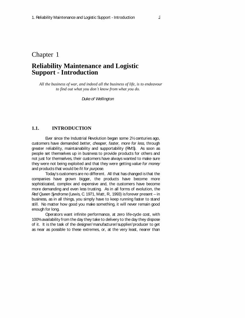
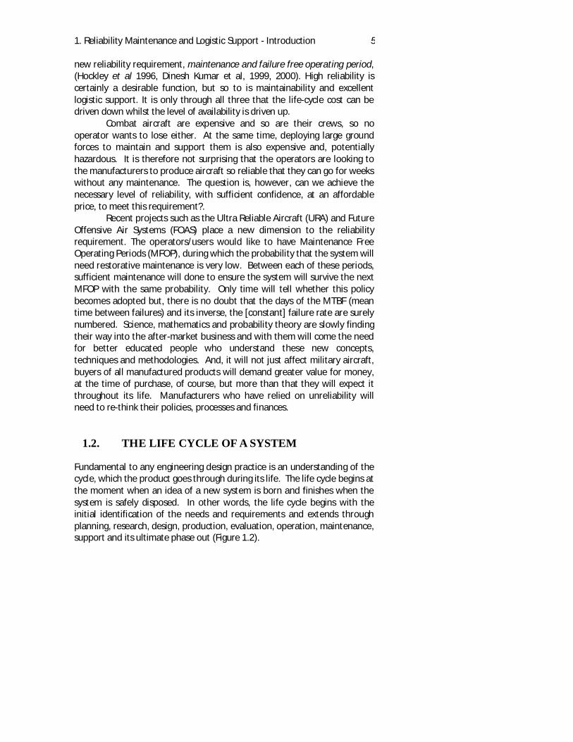
of airliners, such as the Boeing 747, can cost as high as $ 300,000 per day inforfeited revenue alone. Failure to dispatch a commercial flight on time orits cancellation is not only connected to the cost of correcting the failure,but also to the extra crew costs, additional passenger handling and loss ofpassenger revenue. Consequently, this will have an impact on thecompetitiveness, profitability and market share of the airline concerned.'Aircraft on Ground' is probably the most dreaded phrase in the commercialairlines’ vocabulary. And, although the costs and implications may bedifferent, it is no more popular with military operators. Costs per minutedelay for different aircraft type are shown in Figure 1.1. Here the delaycosts are attributable to labour charges, airport fees, air traffic controlcosts, rescheduling costs, passenger costs (food, accommodation, transportand payoffs).
Figure 1.1 Aircraft delay cost per minute
Industries have learned from past experience and through cuttingedge research how to make their products safe and reliable. NASA, Boeing,Airbus, Lockheed Martin, Rolls-Royce, General Electric, Pratt and Whitney,and many, many more, are producing extremely reliable products. Forexample, over 25% of the jetliners in US have been in service for over 20years and more than 500 over 25 years, nearing or exceeding their originaldesign life (Lam, M., 1995). The important message is that these aircraft arestill capable of maintaining their airworthiness; they are still safe andreliable. But, we cannot be complacent, even the best of organisations canhave their bad days. The losses of the Challenger Space Shuttle in 1986, andApollo 13 are still very fresh in many of our memories.Customers’ requirements generally exceed the capabilities of theproducers. Occasionally, these go beyond what is practically, andsometimes even theoretically, possible. An example of this could be the
1. Reliability Maintenance and Logistic Support - Introduction 5
new reliability requirement, maintenance and failure free operating period,(Hockley et al 1996, Dinesh Kumar et al, 1999, 2000). High reliability iscertainly a desirable function, but so to is maintainability and excellentlogistic support. It is only through all three that the life-cycle cost can bedriven down whilst the level of availability is driven up.
Combat aircraft are expensive and so are their crews, so nooperator wants to lose either. At the same time, deploying large groundforces to maintain and support them is also expensive and, potentiallyhazardous. It is therefore not surprising that the operators are looking tothe manufacturers to produce aircraft so reliable that they can go for weekswithout any maintenance. The question is, however, can we achieve thenecessary level of reliability, with sufficient confidence, at an affordableprice, to meet this requirement?.
Recent projects such as the Ultra Reliable Aircraft (URA) and FutureOffensive Air Systems (FOAS) place a new dimension to the reliabilityrequirement. The operators/users would like to have Maintenance FreeOperating Periods (MFOP), during which the probability that the system willneed restorative maintenance is very low. Between each of these periods,sufficient maintenance will done to ensure the system will survive the nextMFOP with the same probability. Only time will tell whether this policybecomes adopted but, there is no doubt that the days of the MTBF (meantime between failures) and its inverse, the [constant] failure rate are surelynumbered. Science, mathematics and probability theory are slowly findingtheir way into the after-market business and with them will come the needfor better educated people who understand these new concepts,techniques and methodologies. And, it will not just affect military aircraft,buyers of all manufactured products will demand greater value for money,at the time of purchase, of course, but more than that they will expect itthroughout its life. Manufacturers who have relied on unreliability willneed to re-think their policies, processes and finances.
1.2. THE LIFE CYCLE OF A SYSTEM
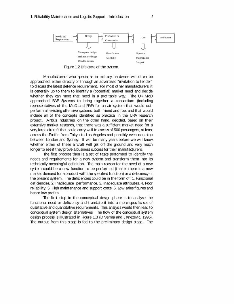
Fundamental to any engineering design practice is an understanding of thecycle, which the product goes through during its life. The life cycle begins atthe moment when an idea of a new system is born and finishes when thesystem is safely disposed. In other words, the life cycle begins with theinitial identification of the needs and requirements and extends throughplanning, research, design, production, evaluation, operation, maintenance,support and its ultimate phase out (Figure 1.2).
1. Reliability Maintenance and Logistic Support - Introduction 6
Figure 1.2 Life cycle of the system.
Manufacturers who specialise in military hardware will often beapproached, either directly or through an advertised “invitation to tender”to discuss the latest defence requirement. For most other manufacturers, itis generally up to them to identify a (potential) market need and decidewhether they can meet that need in a profitable way. The UK MoDapproached BAE Systems to bring together a consortium (includingrepresentatives of the MoD and RAF) for an air system that would out-perform all existing offensive systems, both friend and foe, and that wouldinclude all of the concepts identified as practical in the URA researchproject. Airbus Industries, on the other hand, decided, based on theirextensive market research, that there was a sufficient market need for avery large aircraft that could carry well in excess of 500 passengers, at leastacross the Pacific from Tokyo to Los Angeles and possibly even non-stopbetween London and Sydney. It will be many years before we will knowwhether either of these aircraft will get off the ground and very muchlonger to see if they prove a business success for their manufacturers.
The first process then is a set of tasks performed to identify theneeds and requirements for a new system and transform them into itstechnically meaningful definition. The main reason for the need of a newsystem could be a new function to be performed (that is there is a newmarket demand for a product with the specified function) or a deficiency ofthe present system. The deficiencies could be in the form of: 1. Functionaldeficiencies, 2. Inadequate performance, 3. Inadequate attributes. 4. Poorreliability, 5. High maintenance and support costs, 5. Low sales figures andhence low profits.
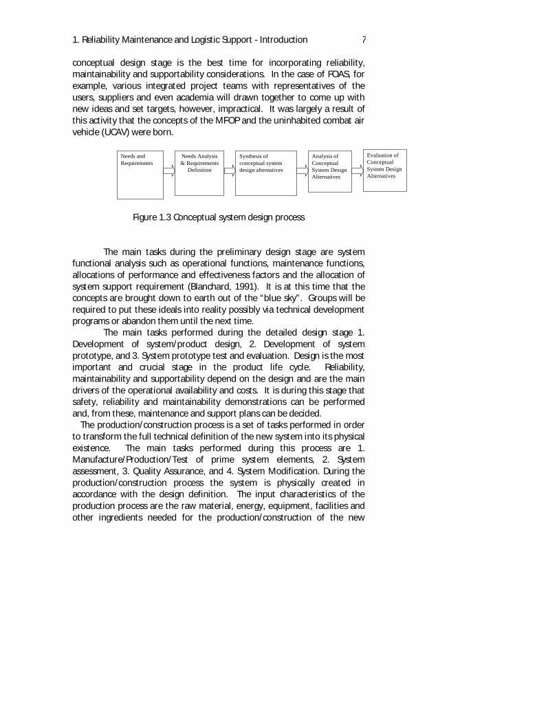
The first step in the conceptual design phase is to analyse thefunctional need or deficiency and translate it into a more specific set ofqualitative and quantitative requirements. This analysis would then lead toconceptual system design alternatives. The flow of the conceptual systemdesign process is illustrated in Figure 1.3 (D Verma and J Knezevic, 1995).The output from this stage is fed to the preliminary design stage. The
Needs andRequirements
Design
Conceptual design
Preliminary design
Detailed design
Production or
Construction
Manufacture
Assembly
Use
Operation
Maintenance
Support
Retirement
1. Reliability Maintenance and Logistic Support - Introduction 7
conceptual design stage is the best time for incorporating reliability,maintainability and supportability considerations. In the case of FOAS, forexample, various integrated project teams with representatives of theusers, suppliers and even academia will drawn together to come up withnew ideas and set targets, however, impractical. It was largely a result ofthis activity that the concepts of the MFOP and the uninhabited combat airvehicle (UCAV) were born.
Figure 1.3 Conceptual system design process
The main tasks during the preliminary design stage are systemfunctional analysis such as operational functions, maintenance functions,allocations of performance and effectiveness factors and the allocation ofsystem support requirement (Blanchard, 1991). It is at this time that theconcepts are brought down to earth out of the “blue sky”. Groups will berequired to put these ideals into reality possibly via technical developmentprograms or abandon them until the next time.
The main tasks performed during the detailed design stage 1.Development of system/product design, 2. Development of systemprototype, and 3. System prototype test and evaluation. Design is the mostimportant and crucial stage in the product life cycle. Reliability,maintainability and supportability depend on the design and are the maindrivers of the operational availability and costs. It is during this stage thatsafety, reliability and maintainability demonstrations can be performedand, from these, maintenance and support plans can be decided.
The production/construction process is a set of tasks performed in orderto transform the full technical definition of the new system into its physicalexistence. The main tasks performed during this process are 1.Manufacture/Production/Test of prime system elements, 2. Systemassessment, 3. Quality Assurance, and 4. System Modification. During theproduction/construction process the system is physically created inaccordance with the design definition. The input characteristics of theproduction process are the raw material, energy, equipment, facilities andother ingredients needed for the production/construction of the new
Needs andRequirements
Needs Analysis& Requirements
Definition
Synthesis ofconceptual systemdesign alternatives
Analysis ofConceptualSystem DesignAlternatives
Evaluation ofConceptualSystem DesignAlternatives
1. Reliability Maintenance and Logistic Support - Introduction 8
system. The output characteristics are the full physical existence of thefunctional system.
1.3. CONCEPT OF FAILURE
As with so many words in the English language, failure has come tomean many things to many people. Essentially, a failure of a system is anyevent or collection of events that causes the system to lose itsfunctionability where functionability is the inherent characteristic of aproduct related to its ability to perform a specified function according to thespecified requirements under the specified operating conditions. (Knezevic1993) Thus a system, or indeed, any component within it, can only be inone of two states: state of functioning or; state of failure.
In many cases, the transition between these states is effectivelyinstantaneous; a windscreen shatters, a tyre punctures, a blade breaks, atransistor blows. There is insufficient time to detect the onset or preventthe consequences. However, in many other cases, the transition is gradual;a tyre or bearing wears, a crack propagates across a disc, a blade “creeps”or the performance starts to drop off. In these circumstances, some formof health monitoring may allow the user to take preventative measures.Inspecting the amount of tread on the tyres at regular intervals, scanningthe lubricating oil for excessive debris, boroscope inspection to look forcracks or using some form trending (e.g. Kalman Filtering) on the specificfuel consumption can alert the user to imminent onset of failure. Similarly,any one of the many forms of non-destructive testing may be used (asappropriate) on components that have been exposed during the recoveryof their parent component to check for damage, deterioration, erosion,corrosion or any of the other visible or physically detectable signs thatmight cause the component to become non-functionable.
With many highly complex systems, whose failure may have seriousor catastrophic consequences, measures are taken, wherever possible, tomitigate against such events. Cars are fitted with dual braking systems,aircraft with (at least) triple hydraulic systems and numerous otherinstances of redundancy. In these cases, it is possible to have a failure of acomponent without a failure of the system. The recovery of the failed item,via a maintenance action, may be deferred to a time which is moreconvenient to the operator, safe in the knowledge that there is anacceptably high probability that the system will continue operating safelyfor a certain length of time. If one of the flight control computers on anaircraft fails, its functions will instantly and automatically be taken over by
1. Reliability Maintenance and Logistic Support - Introduction 9
one of the other computers. The flight will generally be allowed tocontinue, uninterrupted to its next scheduled destination. Depending onthe level of redundancy and regulations/certification, further flights may bepermitted, either until another computer fails or, the aircraft is put in forscheduled maintenance.Most commercial airliners are fitted with two, or more, engines. Part of thecertification process requires a practical demonstration that a fully loadedaircraft can take-off safely even if one of those engines fails at the mostcritical time; “rotation” or “weight-off-wheels”. However, even though theaircraft can fly with one engine out of service, once it has landed, it wouldnot then be permitted to take-off again until that engine has been returnedto a state of functioning (except under very exceptional circumstances).With the latest large twins (e.g. Airbus 330 and Boeing 777), a change in theairworthiness rules has allowed them to fly for extended periods followingthe in-flight shutdown of one of the engines, generally referred to ETOPS(which officially stands for extended twin operations over sea or,unofficially, engines turn or passengers swim). This defines the maximumdistance (usually expressed in minutes of flying time) the aircraft can befrom a suitable landing site at any time during the flight. It also requires anaircraft that has “lost” an engine to fly to immediately divert to a landingsite that is within this flying time. Again, having landed, that aircraft wouldnot be permitted to take off until it was fitted with two functionableengines. In this case, neither engine is truly redundant but, the system(aircraft) has a limited level of fault/failure tolerance.
Most personal computers (PC) come complete with a “hard disc”.During the life of the PC, it is not uncommon for small sectors of these discsto become unusable. Provided the sector did not hold the file access table(FAT) or key system’s files, the computer is not only able to detect thesesectors but it will mark them as unusable and avoid writing any data tothem. Unfortunately, if there was already data on these sectors beforethey become unusable, this will no longer be accessible, although withspecial software, it may be possible to recover some of it. Thus, the built-intest software of the computer is able to provide a level of fault tolerancewhich is often totally invisible to the user, at least until the whole disccrashes or the fault affects a critical part of a program or data. Even underthese circumstances, if that program or data has been backed up to anothermedium, it should be possible to restore the full capacity of the systemusually with a level of manual intervention. So there is both fault toleranceand redundancy although the latter is usually at the discretion of the user.

2. 10
Chapter 2
Probability Theory
We do not know how to predict what would happen in any givencircumstances, and we believe now that it is possible, that the only thing that
can be predicted is the probability of different events
Richard Feynman
Probability theory plays a leading role in modern science in spite of the factthat it was initially developed as a tool that could be used for guessing theoutcome of some games of chance. Probability theory is applicable toeveryday life situations where the outcome of a repeated process,experiment, test, or trial is uncertain and a prediction has to be made.In order to apply probability to everyday engineering practice it is necessaryto learn the terminology, definitions and rules of probability theory. Thischapter is not intended to a rigorous treatment of all-relevant theoremsand proofs. The intention is to provide an understanding of the mainconcepts in probability theory that can be applied to problems in reliability,maintenance and logistic support, which are discussed in the followingchapters.
2.4. PROBABILITY TERMS AND DEFINITIONS
In this section those elements essential for understanding the rudiments ofelementary probability theory will be discussed and defined in a general
2. Probability Theory 11
manner, together with illustrative examples related to engineering practice.To facilitate the discussion some relevant terms and their definitions areintroduced.
Experiment
An experiment is a well-defined act or process that leads to a single well-defined outcome. Figure 2.1 illustrates the concept of random experiments.Every experiment must:
1. Be capable of being described, so that the observer knows when it occurs.2. Have one and only one outcome, so that the set of all possible outcomes
can be specified.
Figure 2.1 Graphical Representation of an Experiment and its outcomes.
Elementary event
An elementary event is every separate outcome of an experiment.
From the definition of an experiment, it is possible to conclude thatthe total number of elementary events is equal to the total number ofpossible outcomes, since every experiment must have only oneoutcome.
Sample space
The set of all possible distinct outcomes for an experiment is calledthe sample space for that experiment.Most frequently in the literature the symbol S is used to represent thesample space, and small letters, a,b,c,.., for elementary events that arepossible outcomes of the experiment under consideration. The set S may
Experiment
2. Probability Theory 12
contain either a finite or an infinite number of elementary events. Figure2.2 is a graphical presentation of the sample space.
Figure 2.2 Graphical Presentation of the Sample Space
Event
Event is a subset of the sample space, that is, a collection ofelementary events.
Capital letters A, B, C, …, are usually used for denoting events. For example,if the experiment performed is measuring the speed of passing cars at aspecific road junction, then the elementary event is the speed measured,whereas the sample space consists of all the different speeds one mightpossibly record. All speed events could be classified in, say, four differentspeed groups: A (less than 30 km/h), B (between 30 and 50 km/h), C(between 50 and 70 km/h) and D (above 70 km/h). If the measured speedof the passing car is, say 35 km/h, then the event B is said to have occurred.
2.5. ELEMENTARY THEORY OF PROBABILITY
The theory of probability is developed from axioms proposed by theRussian mathematician Kolmogrov. In practice this means that its elementshave been defined together with several axioms which govern theirrelations. All other rules and relations are derived from them.
2.5.1 Axioms of Probability
In cases where the outcome of an experiment is uncertain, it isnecessary to assign some measure that will indicate the chances of
2. Probability Theory 13
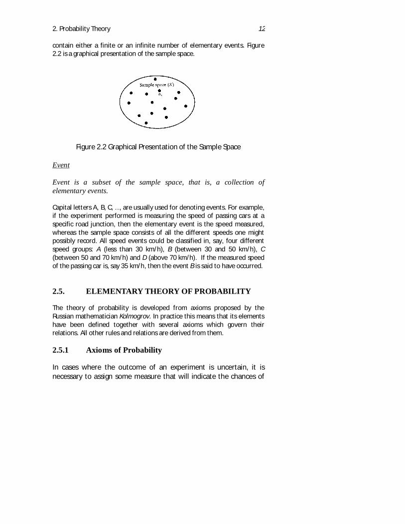
occurrence of a particular event. Such a measure of events is calledthe probability of the event and symbolised by P(.), ( P(A) denotes theprobability of event A). The function which associates each event A inthe sample space S, with the probability measure P(A), is called theprobability function - the probability of that event. A graphicalrepresentation of the probability function is given in Figure 2.3.
Figure 2.3 Graphical representation of probability function.
Formally, the probability function is defined as:
A function which associates with each event A, a real number, P(A),the probability of event A, such that the following axioms are true:
1. P(A) > 0 for every event A,2. P(S) = 1, (probability of the sample space)3. The probability of the union of mutually exclusive events is the sum of
their probabilities, that is
)(...)()()...( 2121 nn APAPAPAAAP +++=∪∪
In essence, this definition states that each event A is paired with a non-negative number, probability P(A), and that the probability of the sureevent S, or P(S), is always 1.Furthermore, if A1 and A2 are any two mutually exclusive events (that is,the occurrence of one event implies the non-occurrence of the other) in the
2. Probability Theory 14
sample space, the probability of their union P A A( )1 2∪ , is simply the sumof their two probabilities, P A P A( ) ( )1 2+ .
2.5.2 Rules of Probability
The following elementary rules of probability are directly deduced from theoriginal three axioms, using the set theory:
a) For any event A, the probability of the complementary event, written A' ,is given by
P A P A( ' ) ( )= −1 (2.1)
b) The probability of any event must lie between zero and one inclusive:
0 1≤ ≤P A( ) (2.2)
c) The probability of an empty or impossible event, φ, is zero.
P( )φ = 0 (2.3)
d) If occurrence of an event A implies that an event B occurs, so that theevent class A is a subset of event class B, then the probability of A is lessthan or equal to the probability of B:
)()( BPAP ≤ (2.4)
e) In order to find the probability that A or B or both occur, the probabilityof A, the probability of B, and also the probability that both occur mustbe known, thus:
P A B P A P B P A B( ) ( ) ( ) ( )∪ = + − ∩ (2.5)
f) If A and B are mutually exclusive events, so that P A B( )∩ = 0 , then
P A B P A P B( ) ( ) ( )∪ = + (2.6)
g) If n events form a partition of S, then their probabilities must add up toone:
2. Probability Theory 15
∑ ==+++=
n
iin APAPAPAP
121 1)()(...)()( (2.7)
2.5.3 Joint Events
Any event that is an intersection of two or more events is a joint event.
There is nothing to restrict any given elementary event from the samplespace from qualifying for two or more events, provided that those eventsare not mutually exclusive. Thus, given the event A and the event B, thejoint event is A B∩ . Since a member of A B∩ must be a member of setA, and also of set B, both A and B events occur when A B∩ occurs.Provided that the elements of set S are all equally likely to occur, theprobability of the joint event could be found in the following way:
P A B( )∩ = ∩number of elementary events in A Btotal number of elementary events
2.5.4 Conditional Probability
If A and B are events in a sample space which consists of a finite number ofelementary events, the conditional probability of the event B given that theevent A has already occurred, denoted by P B A( | ) , is defined as:
P B A P A( | ) , ( )= ∩ >P(A B)P(A)
0 (2.8)
2. Probability Theory 16
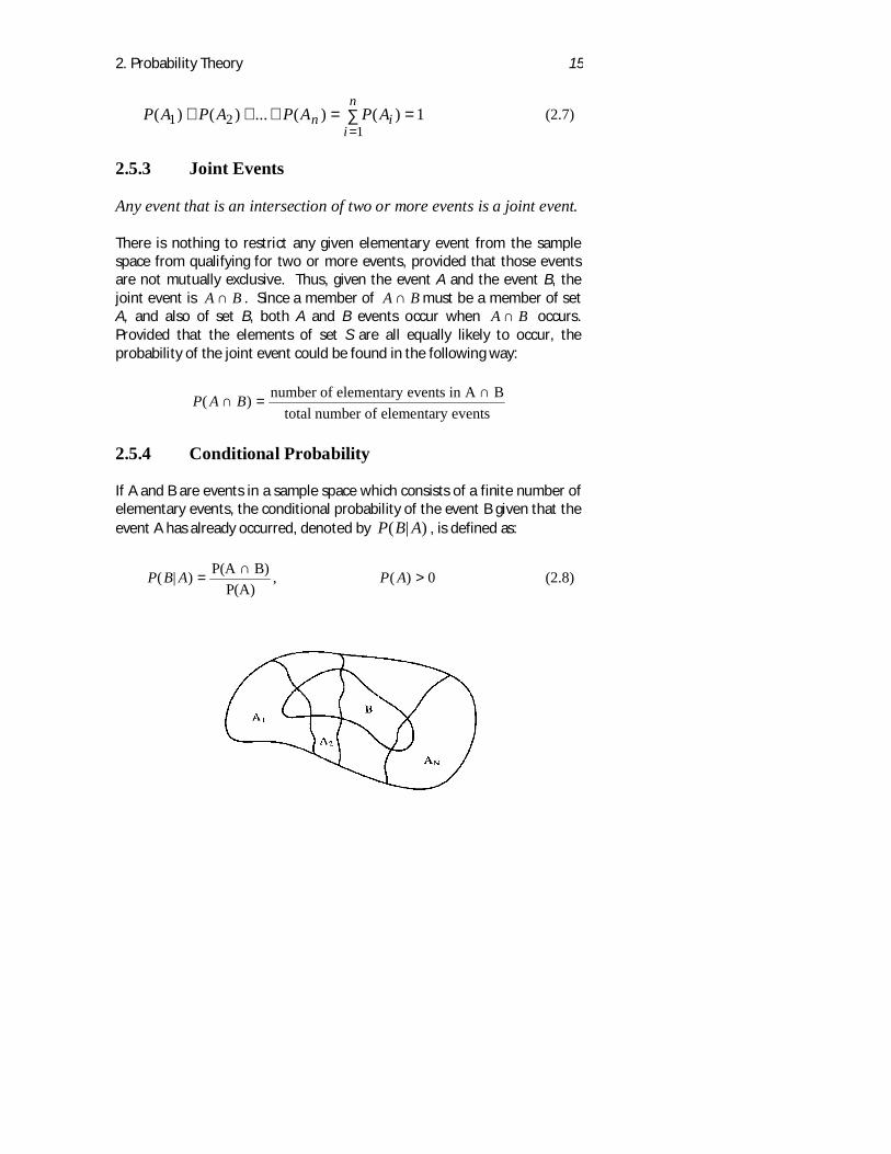
Figure 2.4 Graphical Presentation of the Bayes Theorem
The conditional probability symbol, P B A( | ) , is read as the probability of Bgiven A. It is necessary to satisfy the condition that P(A)>0, because it doesnot make sense to consider the probability of B given A if event A isimpossible. For any two events A and B, there are two conditionalprobabilities that may be calculated:
P B A and P A B( | ) ( | )= ∩ = ∩P(A B)P(A)
P(A B)P(B)
(The probability of B, given A) (The probability of A,given B)
One of the important application of conditional probability is due to Bayestheorem, which can be stated as follows:If ( , , , )A A AN1 2 K represents the partition of the sample space (N
mutually exclusive events), and if B is subset of ( )A A AN1 2∪ ∪ ∪K , asillustrated in Figure 2.4, then
P A Bi( | ) )) ) )
=+ + + +
P(B|A )P(AP(B|A )P(A P(B|A )P(A P(B|A )P(A
i i
1 1 i i N NK K
(2.9)
2.6. PROBABILITY AND EXPERIMENTAL DATA
The classical approach to probability estimation is based on the relativefrequency of the occurrence of that event. A statement of probability tellsus what to expect about the relative frequency of occurrence, given thatenough observations are made. In the long run, the relative frequency ofoccurrence of an event, say A, should approach the probability of thisevent, if independent trials are made at random over an indefinitely longsequence. This principle was first formulated and proved by JamesBernoulli in the early eighteenth century, and is now well-known asBernoulli's theorem:If the probability of occurrence of an event A is p, and if n trials are madeindependently and under the same conditions, then the probability that therelative frequency of occurrence of A, (defined as f A N A n( ) ( )= ) differs
2. Probability Theory 17
from p by any amount, however small, approaches zero as the number oftrials grows indefinitely large. That is,
P N A n p s as n(| ( ) ) | ) ,− > → → ∞0 (2.10)
where s is some arbitrarily small positive number. This does not mean that
the proportion ofnAN )(
occurrences among any n trial must be p; the
proportion actually observed might be any number between 0 and 1.Nevertheless, given more and more trials, the relative frequency of f A( )occurrences may be expected to become closer and closer to p.
Although it is true that the relative frequency of occurrence of any event isexactly equal to the probability of occurrence of any event only for aninfinite number of independent trials, this point must not be over stressed.Even with relatively small number of trials, there is very good reason toexpect the observed relative frequency to be quite close to the probabilitybecause the rate of convergence of the two is very rapid. However, themain drawback of the relative frequency approach is that it assumes that allevents are equally likely (equally probable).
2.7. PROBABILITY DISTRIBUTION
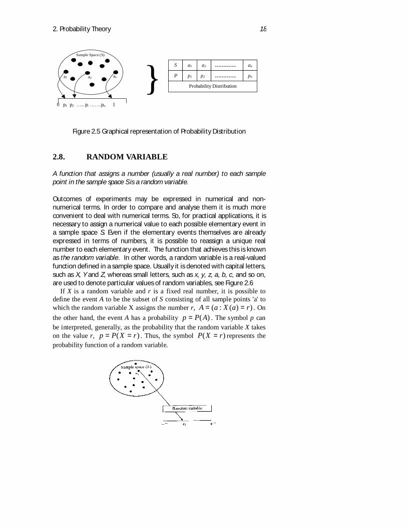
Consider the set of events A A An1 2, , ,K , and suppose that they form apartition of the sample space S. That is, they are mutually exclusive andexhaustive. The corresponding set of probabilities, P A P A P An( ), ( ), , ( )1 2 K ,is a probability distribution. An illustrative presentation of the concept ofprobability distribution is shown in Figure 2.5.As a simple example of a probability distribution, imagine a sample space ofall Ford cars produced. A car selected at random is classified as a saloon orcoupe or estate. The probability distribution might be:
Event Saloon Coupe Estate TotalP 0.60 0.31 0.09 1.00
All events other than those listed have probabilities of zero
2. Probability Theory 18
Figure 2.5 Graphical representation of Probability Distribution
2.8. RANDOM VARIABLE
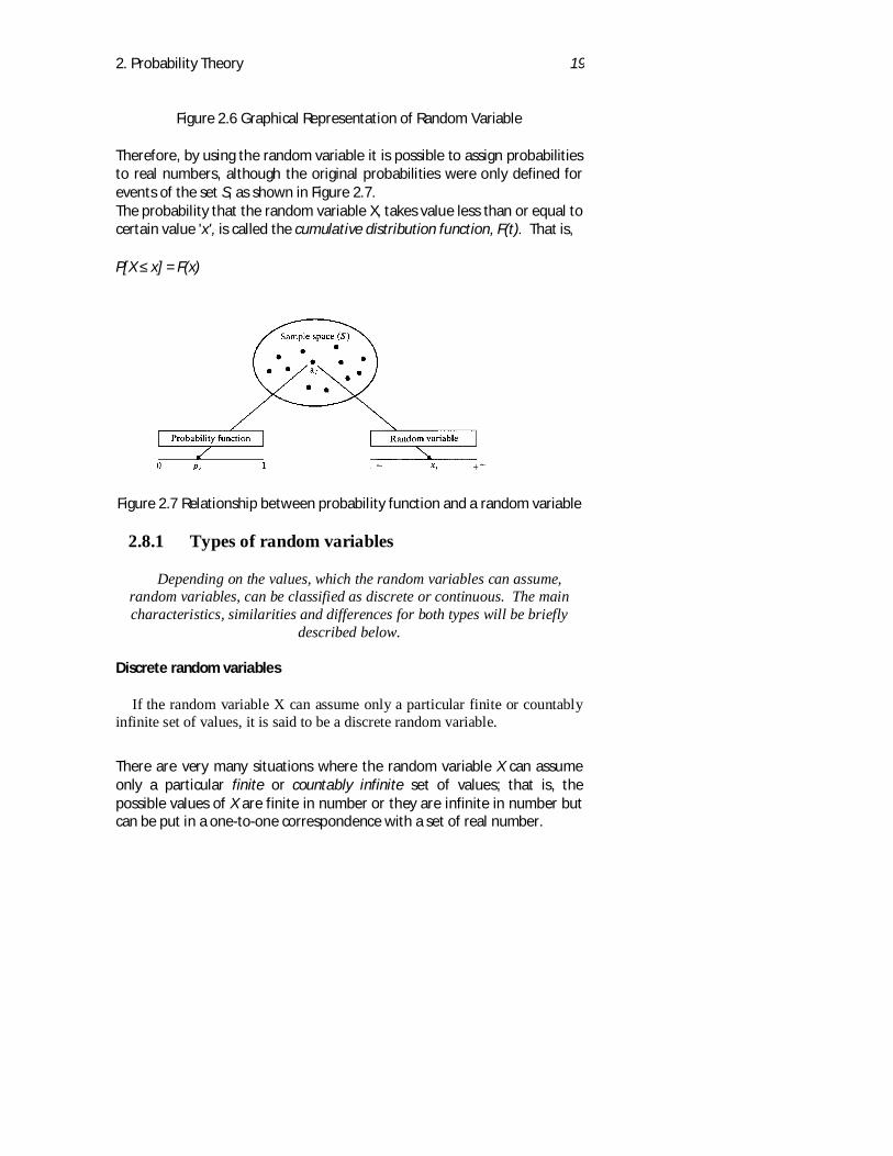
A function that assigns a number (usually a real number) to each samplepoint in the sample space S is a random variable.
Outcomes of experiments may be expressed in numerical and non-numerical terms. In order to compare and analyse them it is much moreconvenient to deal with numerical terms. So, for practical applications, it isnecessary to assign a numerical value to each possible elementary event ina sample space S. Even if the elementary events themselves are alreadyexpressed in terms of numbers, it is possible to reassign a unique realnumber to each elementary event. The function that achieves this is knownas the random variable. In other words, a random variable is a real-valuedfunction defined in a sample space. Usually it is denoted with capital letters,such as X, Y and Z, whereas small letters, such as x, y, z, a, b, c, and so on,are used to denote particular values of random variables, see Figure 2.6
If X is a random variable and r is a fixed real number, it is possible todefine the event A to be the subset of S consisting of all sample points 'a' towhich the random variable X assigns the number r, ))(:( raXaA == . Onthe other hand, the event A has a probability )(APp = . The symbol p canbe interpreted, generally, as the probability that the random variable X takeson the value r, )( rXPp == . Thus, the symbol )( rXP = represents theprobability function of a random variable.
0 p1 p2 .. pi .pn 1
Sample Space (S)
a1 a2 an } Probability Distribution
S
P
a1
p1
a2
p2
.
.
an
pn
2. Probability Theory 19
Figure 2.6 Graphical Representation of Random Variable
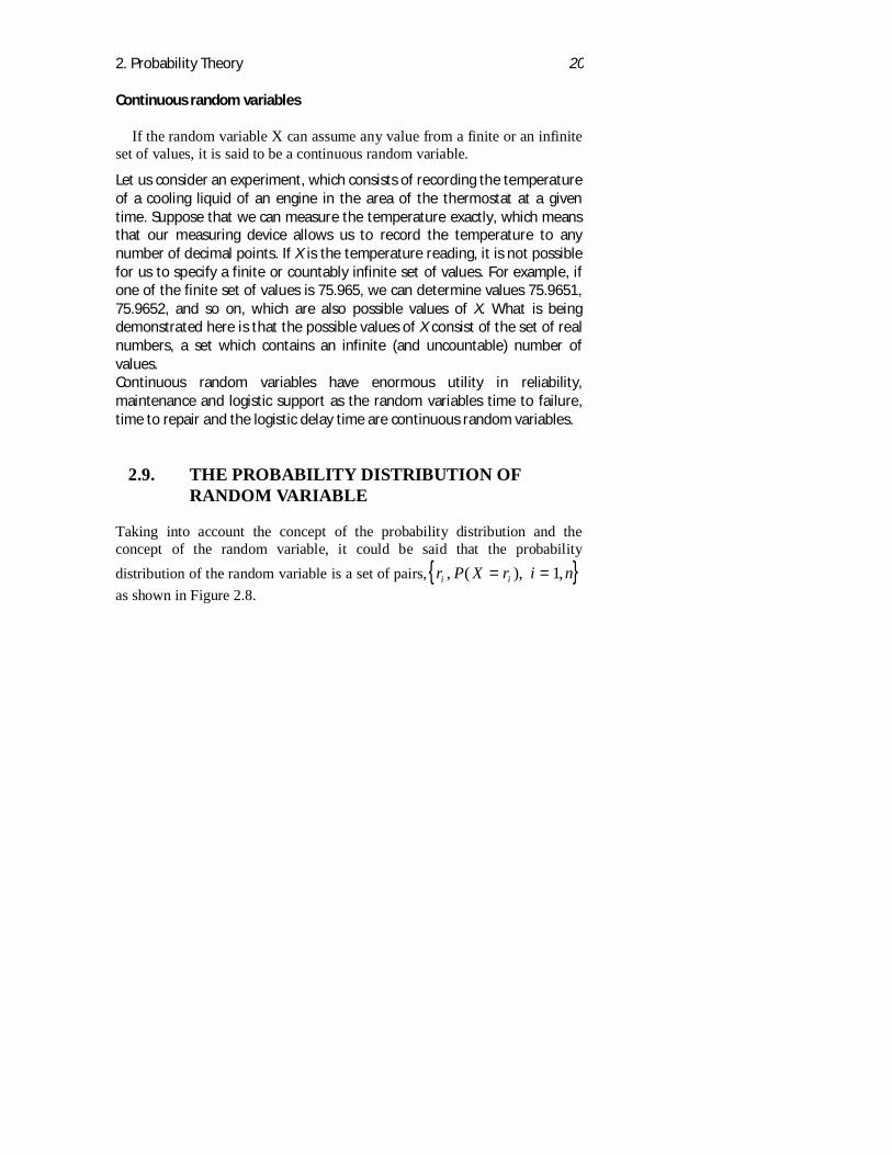
Therefore, by using the random variable it is possible to assign probabilitiesto real numbers, although the original probabilities were only defined forevents of the set S, as shown in Figure 2.7.The probability that the random variable X, takes value less than or equal tocertain value 'x', is called the cumulative distribution function, F(t). That is,
P[X ≤ x] = F(x)
Figure 2.7 Relationship between probability function and a random variable
2.8.1 Types of random variables
Depending on the values, which the random variables can assume,random variables, can be classified as discrete or continuous. The maincharacteristics, similarities and differences for both types will be briefly
described below.
Discrete random variables
If the random variable X can assume only a particular finite or countablyinfinite set of values, it is said to be a discrete random variable.
There are very many situations where the random variable X can assumeonly a particular finite or countably infinite set of values; that is, thepossible values of X are finite in number or they are infinite in number butcan be put in a one-to-one correspondence with a set of real number.
2. Probability Theory 20
Continuous random variables
If the random variable X can assume any value from a finite or an infiniteset of values, it is said to be a continuous random variable.
Let us consider an experiment, which consists of recording the temperatureof a cooling liquid of an engine in the area of the thermostat at a giventime. Suppose that we can measure the temperature exactly, which meansthat our measuring device allows us to record the temperature to anynumber of decimal points. If X is the temperature reading, it is not possiblefor us to specify a finite or countably infinite set of values. For example, ifone of the finite set of values is 75.965, we can determine values 75.9651,75.9652, and so on, which are also possible values of X. What is beingdemonstrated here is that the possible values of X consist of the set of realnumbers, a set which contains an infinite (and uncountable) number ofvalues.Continuous random variables have enormous utility in reliability,maintenance and logistic support as the random variables time to failure,time to repair and the logistic delay time are continuous random variables.
2.9. THE PROBABILITY DISTRIBUTION OFRANDOM VARIABLE
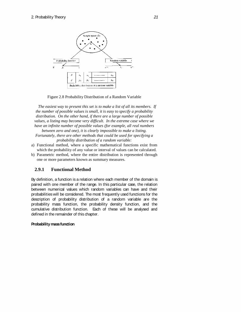
Taking into account the concept of the probability distribution and theconcept of the random variable, it could be said that the probabilitydistribution of the random variable is a set of pairs,{ }r P X r i ni i, ( ), ,= = 1as shown in Figure 2.8.
2. Probability Theory 21
Figure 2.8 Probability Distribution of a Random Variable
The easiest way to present this set is to make a list of all its members. Ifthe number of possible values is small, it is easy to specify a probabilitydistribution. On the other hand, if there are a large number of possible
values, a listing may become very difficult. In the extreme case where wehave an infinite number of possible values (for example, all real numbers
between zero and one), it is clearly impossible to make a listing.Fortunately, there are other methods that could be used for specifying a
probability distribution of a random variable:a) Functional method, where a specific mathematical functions exist from
which the probability of any value or interval of values can be calculated.b) Parametric method, where the entire distribution is represented through
one or more parameters known as summary measures.
2.9.1 Functional Method
By definition, a function is a relation where each member of the domain ispaired with one member of the range. In this particular case, the relationbetween numerical values which random variables can have and theirprobabilities will be considered. The most frequently used functions for thedescription of probability distribution of a random variable are theprobability mass function, the probability density function, and thecumulative distribution function. Each of these will be analysed anddefined in the remainder of this chapter.
Probability mass function
2. Probability Theory 22
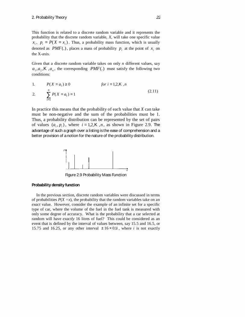
This function is related to a discrete random variable and it represents theprobability that the discrete random variable, X, will take one specific valuexi , p P X xi i= =( ) . Thus, a probability mass function, which is usuallydenoted as PMF(.) , places a mass of probability pi at the point of xi onthe X-axis.
Given that a discrete random variable takes on only n different values, saya a an1 2, , ,K , the corresponding PMF(.) must satisfy the following twoconditions:
1 0 1 2
2 11
. ( ) , , ,
. ( )
P X a for i n
P X a
i
ii
n
= ≥ =
= ==∑
K
(2.11)
In practice this means that the probability of each value that X can takemust be non-negative and the sum of the probabilities must be 1.Thus, a probability distribution can be represented by the set of pairsof values ( , )a pi i , where i n= 1 2, , ,K , as shown in Figure 2.9. Theadvantage of such a graph over a listing is the ease of comprehension and abetter provision of a notion for the nature of the probability distribution.
Figure 2.9 Probability Mass Function
Probability density function
In the previous section, discrete random variables were discussed in termsof probabilities P(X =x), the probability that the random variables take on anexact value. However, consider the example of an infinite set for a specifictype of car, where the volume of the fuel in the fuel tank is measured withonly some degree of accuracy. What is the probability that a car selected atrandom will have exactly 16 litres of fuel? This could be considered as anevent that is defined by the interval of values between, say 15.5 and 16.5, or15.75 and 16.25, or any other interval ± ×16 01. i , where i is not exactly
2. Probability Theory 23
zero. Since the smaller the interval, the smaller the probability, theprobability of exactly 16 litres is, in effect, zero.
In general, for continuous random variables, the occurrence of any exactvalue of X may be regarded as having zero probability.
The Probability Density Function, )(xf , which represents the probabilitythat the random variable will take values within the intervalx X x x≤ ≤ + ∆( ) , when ∆( )x approaches zero, is defined as:
f x P x X x xxx
( ) lim ( ( ))( )
= ≤ ≤ +→∆
∆∆0
(2.12)
As a consequence, the probabilities of a continuous random variable can bediscussed only for intervals of X values. Thus, instead of the probability thatX takes on a specific value, say 'a', we deal with the so-called probabilitydensity of X at 'a', symbolised by f a( ) . In general, the probabilitydistribution of a continuous random variable can be represented by itsProbability Density Function, PDF, which is defined in the following way:
P a X b f x dxa
b
( ) ( )≤ ≤ = ∫ (2.13)
A fully defined probability density function must satisfy the following tworequirements:
f x for all x( ) ≥ 0
f x dx( )−∞
+∞
∫ = 1
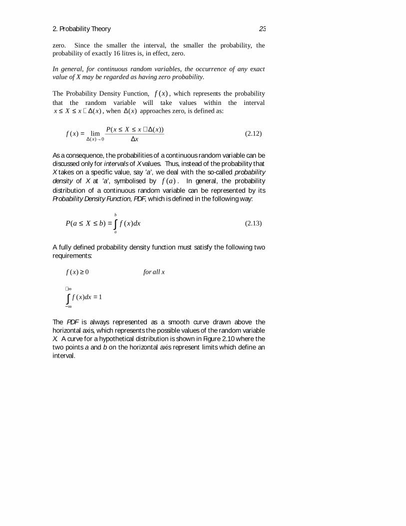
The PDF is always represented as a smooth curve drawn above thehorizontal axis, which represents the possible values of the random variableX. A curve for a hypothetical distribution is shown in Figure 2.10 where thetwo points a and b on the horizontal axis represent limits which define aninterval.
2. Probability Theory 24
Figure 2.10 Probability Density Function for a Hypothetical Distribution
The shaded portion between 'a' and 'b' represents the probability that Xtakes on a value between the limits 'a' and 'b'.
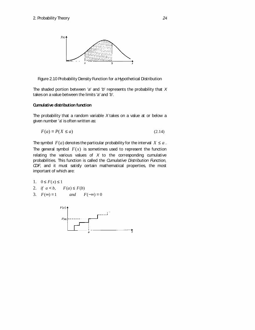
Cumulative distribution function
The probability that a random variable X takes on a value at or below agiven number 'a' is often written as:
)()( aXPaF ≤= (2.14)
The symbol )(aF denotes the particular probability for the interval aX ≤ .
The general symbol )(xF is sometimes used to represent the functionrelating the various values of X to the corresponding cumulativeprobabilities. This function is called the Cumulative Distribution Function,CDF, and it must satisfy certain mathematical properties, the mostimportant of which are:
1. 0 1≤ ≤F x( )2. if a b F a F b< ≤, ( ) ( )3. F and F( ) ( )∞ = −∞ =1 0
2. Probability Theory 25
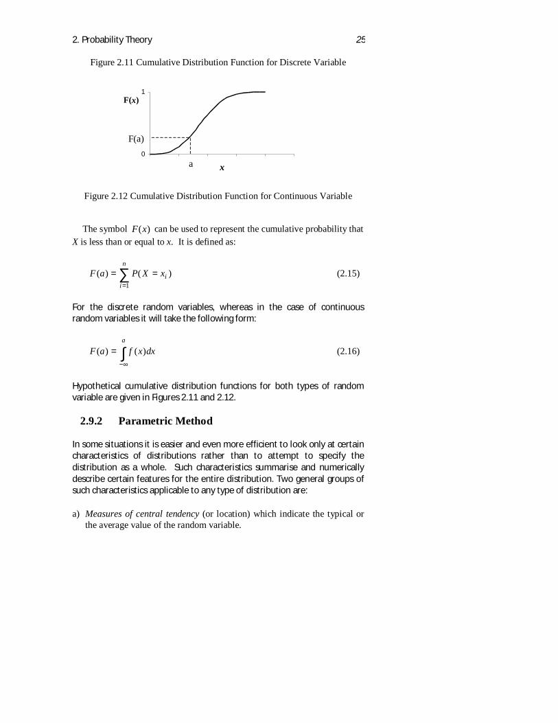
Figure 2.11 Cumulative Distribution Function for Discrete Variable
Figure 2.12 Cumulative Distribution Function for Continuous Variable
The symbol F x( ) can be used to represent the cumulative probability thatX is less than or equal to x. It is defined as:
F a P X xii
n( ) ( )= =
=∑
1
(2.15)
For the discrete random variables, whereas in the case of continuousrandom variables it will take the following form:
F a f x dxa
( ) ( )=−∞∫ (2.16)
Hypothetical cumulative distribution functions for both types of randomvariable are given in Figures 2.11 and 2.12.
2.9.2 Parametric Method
In some situations it is easier and even more efficient to look only at certaincharacteristics of distributions rather than to attempt to specify thedistribution as a whole. Such characteristics summarise and numericallydescribe certain features for the entire distribution. Two general groups ofsuch characteristics applicable to any type of distribution are:
a) Measures of central tendency (or location) which indicate the typical orthe average value of the random variable.
0
1
x
F(x)
a
F(a)
2. Probability Theory 26
b) Measures of dispersion (or variability) which show the spread of thedifference among the possible values of the random variable.
In many cases, it is possible to adequately describe a probability distributionwith a few measures of this kind. It should be remembered, however, thatthese measures serve only to summarise some important features of theprobability distribution. In general, they do not completely describe theentire distribution.One of the most common and useful summary measures of a probabilitydistribution is the expectation of a random variable, E(X). It is a uniquevalue that indicates a location for the distribution as a whole (In physicalscience, expected value actually represents the Centre of gravity). Theconcept of expectation plays an important role not only as a usefulmeasure, but also as a central concept within the theory of probability andstatistics.If a random variable, say X, is discrete, then its expectation is defined as:
∑ =×=x
xXPxXE )()( (2.17)
Where the sum is taken for all the values that the variable X can assume. Ifthe random variable is continuous, the expectation is defined as:
∫+∞
∞−
×= dxxfxXE )()( (2.18)
Where the sum is taken over all values that X can assume. For a continuousrandom variable the expectation is defined as:
E X F x dx( ) [ ( )]= −−∞
+∞
∫ 1 (2.19)
If c is a constant, then
)()( XEccXE ×= (2.20)
Also, for any two random variables X and Y,
)()()( YEXEYXE +=+
2. Probability Theory 27
Measures of central tendency
The most frequently used measures are:
The mean of a random variable is simply the expectation of the randomvariable under consideration. Thus, for the random variable, X, the meanvalue is defined as:
)(XEMean = (2.21)
The median, is defined as the value of X which is midway (in terms ofprobability) between the smallest possible value and the largest possiblevalue. The median is the point, which divides the total area under the PDFinto two equal parts. In other words, the probability that X is less than themedian is1 2 , and the probability that X is greater than the median is also1 2 . Thus, if P X a( ) .≤ ≥ 050 and P X a( ) .≥ ≥ 050 then 'a' is themedian of the distribution of X. In the continuous case, this can be expressedas:
f x dx f x dxa
a
( ) ( ) .−∞
+∞
∫ ∫= = 0 50 (2.22)
The mode, is defined as the value of X at which the PDF of X reaches itshighest point. If a graph of the PMF (PDF), or a listing of possible values of Xalong with their probabilities is available, determination of the mode isquite simple.
A central tendency parameter, whether it is mode, median, mean, or anyother measure, summarises only a certain aspect of a distribution. It is easyto find two distributions which have the same mean but which are not at allsimilar in any other respect.
Measures of dispersion
The mean is a good indication of the location of a random variable, but nosingle value need be exactly like the mean. A deviation from the mean, D,expresses the measure of error made by using the mean as a particularvalue:
2. Probability Theory 28
MxD −=
Where, x, is a possible value of the random variable, X. The deviation canbe taken from other measures of central tendency such as the median ormode. It is quite obvious that the larger such deviations are from ameasure of central tendency, the more the individual values differ fromeach other, and the more apparent the spread within the distributionbecomes. Consequently, it is necessary to find a measure that will reflectthe spread, or variability, of individual values.The expectation of the deviation about the mean as a measure ofvariability, E(X - M), will not work because the expected deviation from themean must be zero for obvious reasons. The solution is to find the square ofeach deviation from the mean, and then to find the expectation of thesquared deviation. This characteristic is known as a variance of thedistribution, V, thus:
V X E X Mean X Mean P x( ) ( ) ( ) ( )= − = − ×∑2 2 if X is discrete (2.23)
V X E X Mean X Mean f x dx( ) ( ) ( ) ( )= − = − ×−∞
+∞
∫2 2 if X is continuous (2.24)
The positive square root of the variance for a distribution is called theStandard Deviation, SD.
)(XVSD = (2.25)
Probability distributions can be analysed in greater depth by introducingother summary measures, known as moments. Very simply these areexpectations of different powers of the random variable. More informationabout them can be found in texts on probability.
2. Probability Theory 29
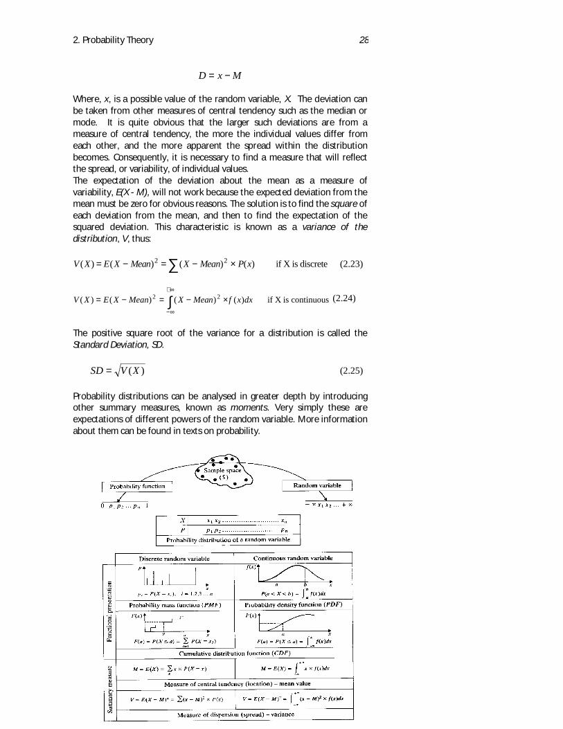
Figure 2.13 Probability System for Continuous Random Variable
Variability
The standard deviation is a measure that shows how closely the values ofrandom variables are concentrated around the mean. Sometimes it isdifficult to use only knowledge of the standard deviation, to decide whetherthe dispersion is considerably large or small, because this will depend onthe mean value. In this case the parameter known as coefficient ofvariation, CVX , defined as
MSDCVX = (2.26)
Coefficient of variation is very useful because it gives better informationregarding the dispersion. The concept thus discussed so far is summarisedin Figure 2.13.In conclusion it could be said that the probability system is wholly abstractand axiomatic. Consequently, every fully defined probability problem has aunique solution.
2.10. DISCRETE THEORETICAL PROBABILITYDISTRIBUTIONS
In probability theory, there are several rules that define the functionalrelationship between the possible values of random variable X and theirprobabilities, P(X). As they are purely theoretical, i.e. they do not exist inreality, they are called theoretical probability distributions. Instead ofanalysing the ways in which these rules have been derived, the analysis inthis chapter concentrates on their properties. It is necessary to emphasisethat all theoretical distributions represent the family of distributionsdefined by a common rule through unspecified constants known asparameters of distribution. The particular member of the family is definedby fixing numerical values for the parameters, which define the distribution.
2. Probability Theory 30
The probability distributions most frequently used in reliability,maintenance and the logistic support are examined in this chapter.Among the family of theoretical probability distributions that are related todiscrete random variables, the Binomial distribution and the Poissondistribution are relevant to the objectives set by this book. A briefdescription of each now follows.
2.10.1 Bernuolli Trials
The simple probability distribution is one with only two event classes. Forexample, a car is tested and one of two events, pass or fail, must occur,each with some probability. The type of experiment consisting of series ofindependent trials, each of which can eventuate in only one of twooutcomes are known as Bernuolli Trials, and the two event classes and theirassociated probabilities a Bernuolli Process. In general, one of the twoevents is called a “success” and the other a “failure” or “nonsuccess”.These names serve only to tell the events apart, and are not meant to bearany connotation of “goodness” of the event. The symbol p, stands for theprobability of a success, q for the probability of failure (p + q =1). If 5independent trials are made (n = 5), then 25 = 32 different sequences ofpossible outcomes would be observed.The probability of given sequences depends upon p and q, the probability ofthe two events. Fortunately, since trials are independent, it is possible tocompute the probability of any sequence.If all possible sequences and their probabilities, are written down thefollowing fact emerges: The probability of any given sequences of nindependent Bernuolli Trials depends only on the number of successes andp. This is regardless of the order in which successes and failure occur insequence, the probability is
p qr n r−
where r is the number of successes, and n r− is the number of failures.Suppose that in a sequence of 10 trials, exactly 4 success occurs. Then theprobability of that particular sequence is p q4 6 . If
32=p , then the
probability can worked out from:23
13
4 6
2. Probability Theory 31
The same procedure would be followed for any r successes out of n trialsfor any p. Generalising this idea for any r, n, and p, we have the followingprinciple:In sampling from the Bernuolli Process with the probability of a successequal to p, the probability of observing exactly r successes in n independenttrials is:
P r successes n pnr p q
nr n r
p qr n r r n r( | , )!
!( )!=
=
−− − (2.27)
2.10.2 The Binomial Distribution
The theoretical probability distribution, which pairs the number of successesin n trials with its probability, is called the binominal distribution.
This probability distribution is related to experiments, which consist of aseries of independent trials, each of which can result in only one of twooutcomes: success and or failure. These names are used only to tell theevents apart. By convention the symbol p stands for the probability of asuccess, q for the probability of failure ( )p q+ = 1 .
The number of successes, x in n trials is a discrete random variable whichcan take on only the whole values from 0 through n. The PMF of theBinomial distribution is given by:
PMF x P X xnx
p q x nx n x( ) ( ) ,= = =
< <− 0 (2.28)
where:
nx
p q nx n x
p qx n x x n x
=
−− −!
!( )!(2.29)
The binomial distribution expressed in cumulative form, representing theprobability that X falls at or below a certain value 'a' is defined by thefollowing equation:
2. Probability Theory 32
P X a P X xni
p qii n i
i
a
i o
a( ) ( )≤ = = =
−
==∑∑
0
(2.30)
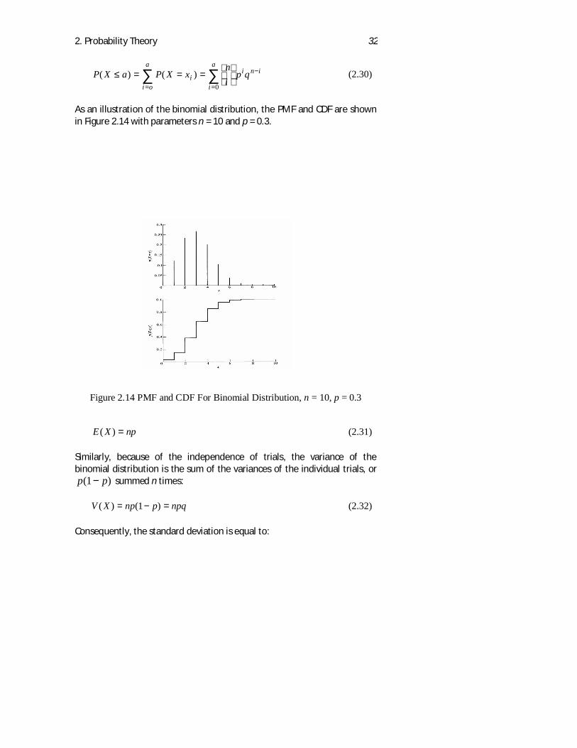
As an illustration of the binomial distribution, the PMF and CDF are shownin Figure 2.14 with parameters n = 10 and p = 0.3.
Figure 2.14 PMF and CDF For Binomial Distribution, n = 10, p = 0.3
E X np( ) = (2.31)
Similarly, because of the independence of trials, the variance of thebinomial distribution is the sum of the variances of the individual trials, orp p( )1− summed n times:
V X np p npq( ) ( )= − =1 (2.32)
Consequently, the standard deviation is equal to:
2. Probability Theory 33
Sd X npq( ) = (2.33)
Although the mathematical rule for the binomial distribution is the sameregardless of the particular values which parameters n and p take, theshape of the probability mass function and the cumulative distributionfunction will depend upon them. The PMF of the binomial distribution issymmetric if p = 0.5, positively skewed if p < 0.5, and negatively skewed if p> 0.5.
2.10.3 The Poisson Distribution
The theoretical probability distribution which pairs the number ofoccurrences of an event in a given time period with its probability is calledthe Poisson distribution. There are experiments where it is not possible toobserve a finite sequence of trials. Instead, observations take place over acontinuum, such as time. For example, if the number of cars arriving at aspecific junction in a given period of time is observed, say for one minute, itis difficult to think of this situation in terms of finite trials. If the number ofbinomial trials n, is made larger and larger and p smaller and smaller in sucha way that np remains constant, then the probability distribution of thenumber of occurrences of the random variable approaches the Poissondistribution.The probability mass function in the case of the Poisson distribution forrandom variable X can be expressed as follows:
P X xe
x
x
( | )!
= =−
λλλ
where x = 0, 1, 2, (2.34)
λ is the intensity of the process and represents the expected number ofoccurrences in a time period of length t. Figure 2.15 shows the PMF of thePoisson distribution with λ = 5
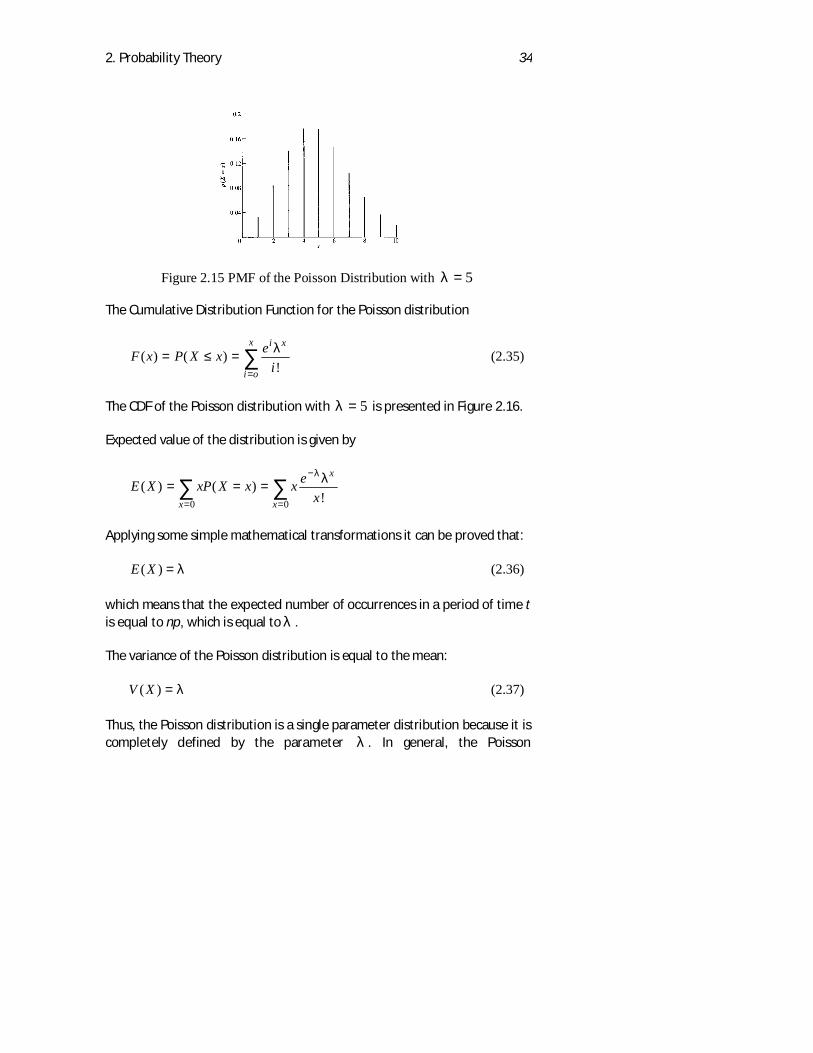
2. Probability Theory 34
Figure 2.15 PMF of the Poisson Distribution with λ = 5
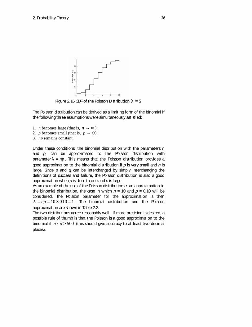
The Cumulative Distribution Function for the Poisson distribution
F x P X x ei
i x
i o
x( ) ( )
!= ≤ =
=∑ λ (2.35)
The CDF of the Poisson distribution with λ = 5 is presented in Figure 2.16.
Expected value of the distribution is given by
E X xP X x x exx
x
x
( ) ( )!
= = ==
−
=∑ ∑
0 0
λ λ
Applying some simple mathematical transformations it can be proved that:
E X( ) = λ (2.36)
which means that the expected number of occurrences in a period of time tis equal to np, which is equal to λ .
The variance of the Poisson distribution is equal to the mean:
V X( ) = λ (2.37)
Thus, the Poisson distribution is a single parameter distribution because it iscompletely defined by the parameter λ . In general, the Poisson

2. Probability Theory 35
distribution is positively skewed, although it is nearly symmetrical asλ becomes larger.
2. Probability Theory 36
Figure 2.16 CDF of the Poisson Distribution λ = 5
The Poisson distribution can be derived as a limiting form of the binomial ifthe following three assumptions were simultaneously satisfied:
1. n becomes large (that is, n → ∞ ).2. p becomes small (that is, p → 0).3. np remains constant.
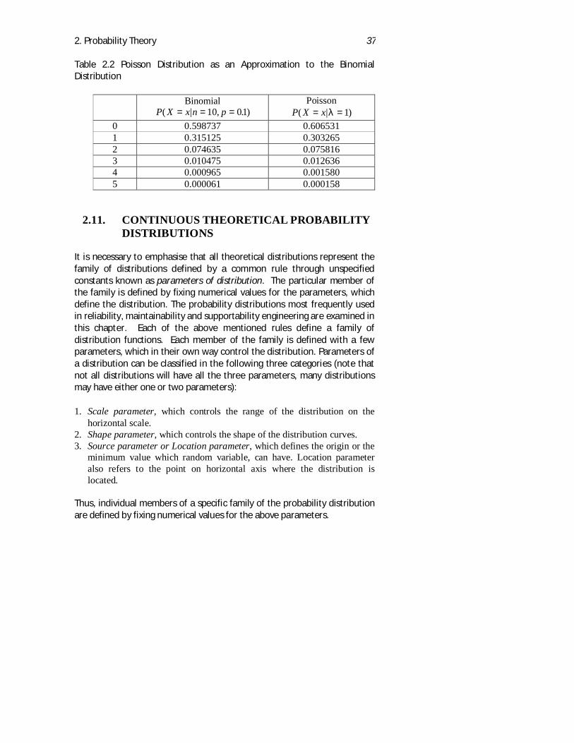
Under these conditions, the binomial distribution with the parameters nand p, can be approximated to the Poisson distribution withparameter λ = np . This means that the Poisson distribution provides agood approximation to the binomial distribution if p is very small and n islarge. Since p and q can be interchanged by simply interchanging thedefinitions of success and failure, the Poisson distribution is also a goodapproximation when p is close to one and n is large.As an example of the use of the Poisson distribution as an approximation tothe binomial distribution, the case in which n = 10 and p = 0.10 will beconsidered. The Poisson parameter for the approximation is thenλ = = × =np 10 010 1. . The binomial distribution and the Poissonapproximation are shown in Table 2.2.The two distributions agree reasonably well. If more precision is desired, apossible rule of thumb is that the Poisson is a good approximation to thebinomial if n p/ > 500 (this should give accuracy to at least two decimalplaces).
2. Probability Theory 37
Table 2.2 Poisson Distribution as an Approximation to the BinomialDistribution
BinomialP X x n p( | , . )= = =10 01
PoissonP X x( | )= =λ 1
0 0.598737 0.6065311 0.315125 0.3032652 0.074635 0.0758163 0.010475 0.0126364 0.000965 0.0015805 0.000061 0.000158
2.11. CONTINUOUS THEORETICAL PROBABILITYDISTRIBUTIONS
It is necessary to emphasise that all theoretical distributions represent thefamily of distributions defined by a common rule through unspecifiedconstants known as parameters of distribution. The particular member ofthe family is defined by fixing numerical values for the parameters, whichdefine the distribution. The probability distributions most frequently usedin reliability, maintainability and supportability engineering are examined inthis chapter. Each of the above mentioned rules define a family ofdistribution functions. Each member of the family is defined with a fewparameters, which in their own way control the distribution. Parameters ofa distribution can be classified in the following three categories (note thatnot all distributions will have all the three parameters, many distributionsmay have either one or two parameters):
1. Scale parameter, which controls the range of the distribution on thehorizontal scale.
2. Shape parameter, which controls the shape of the distribution curves.3. Source parameter or Location parameter, which defines the origin or the
minimum value which random variable, can have. Location parameteralso refers to the point on horizontal axis where the distribution islocated.
Thus, individual members of a specific family of the probability distributionare defined by fixing numerical values for the above parameters.
2. Probability Theory 38
2.11.1 Exponential Distribution
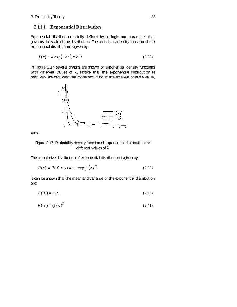
Exponential distribution is fully defined by a single one parameter thatgoverns the scale of the distribution. The probability density function of theexponential distribution is given by:
( ) 0,exp)( >−= xxxf λλ (2.38)
In Figure 2.17 several graphs are shown of exponential density functionswith different values of λ. Notice that the exponential distribution ispositively skewed, with the mode occurring at the smallest possible value,
zero.
Figure 2.17. Probability density function of exponential distribution fordifferent values of λ
The cumulative distribution of exponential distribution is given by:
( )( )xxXPxF λ−−=<= exp1)()( (2.39)
It can be shown that the mean and variance of the exponential distributionare:
λ/1)( =XE (2.40)
2)/1()( λ=XV (2.41)
2. Probability Theory 39
The standard deviation in the case of the exponential distribution rule has anumerical value identical to the mean and the scale parameter,
λ/1)()( == XEXSD .
11.1.1 Memory-less Property of Exponential Distribution
One of the unique property of exponential distribution is that it is the onlycontinuous distribution that has memory less property. Suppose that therandom variable X measures the duration of time until the occurrence offailure of an item and that it is known that X has an exponential distributionwith parameter λ. Suppose the present age of the item is t, that is X > t.Assume that we are interested in finding the probability that this item willnot fail for another s units of time. This can be expressed using theconditional probability as:
}{ txtsXP >+>
Using conditional probability of events, the above probability can bewritten as:
}{}{
}{}{}{
tXPtsXP
tXPtXtsXPsXtsXP
>+>
=>
>∩+>=>+> (2.42)
However we know that for exponential distribution
))(exp(][ tstsXP +−=+> λ and )exp(][ ttXP λ−=>
Substituting these expressions in equation (2.42), we get
)exp(][][ ssXPtXtsXP λ−=>=>+>
That is, the conditional probability depends only on the remaining durationand is independent of the current age of the item. This property is exploitedto a great extend in reliability theory.
2.11.2 Normal Distribution (Gaussian Distribution)
This is the most frequently used and most extensively covered theoreticaldistribution in the literature. The Normal Distribution is continuous for allvalues of X between − ∞ and + ∞ . It has a characteristic symmetrical
2. Probability Theory 40
shape, which means that the mean, the median and the mode have thesame numerical value. The mathematical expression for its probabilitydensity function is as follows:
−
−=2
21exp
21)(
σµ
πσxxf (2.43)
Where µ is a location parameter (as it locates the distribution on thehorizontal axis) and σ is a scale parameter (as it controls the range of thedistribution). µ and σ also represents the mean and the standard deviationof this distribution.The influence of the parameter µ on the location of the distribution on thehorizontal axis is shown in Figure 2.18, where the values for parameter σare constant.As the deviation of x from the location parameter µ is entered as a squaredquantity, two different x values, showing the same absolute deviation fromµ, will have the same probability density according to this rule. This dictatesthe symmetry of the normal distribution. Parameter µ can be any finitenumber, while σ can be any positive finite number.
The cumulative distribution function for the normal distribution is:
F a P X a f x dxa
( ) ( ) ( )= ≤ =−∞∫
where f(x) is the normal density function. Taking into account Eq. (2.43)this becomes:
dxaaFa∫
−
−=∞−
2
21exp
21)(
σµ
πσ(2.44)
2. Probability Theory 41
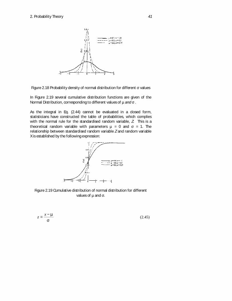
Figure 2.18 Probability density of normal distribution for different σ values
In Figure 2.19 several cumulative distribution functions are given of theNormal Distribution, corresponding to different values of µ and σ .
As the integral in Eq. (2.44) cannot be evaluated in a closed form,statisticians have constructed the table of probabilities, which complieswith the normal rule for the standardised random variable, Z. This is atheoretical random variable with parameters µ = 0 and σ = 1. Therelationship between standardised random variable Z and random variableX is established by the following expression:
Figure 2.19 Cumulative distribution of normal distribution for differentvalues of µ and σ.
σµ−
=xz (2.45)
2. Probability Theory 42
Making use of the above expression the equation (2.43) becomessimpler:
2
21
21)(
zezf
−=
πσ(2.46)
The standardised form of the distribution makes it possible to use only onetable for the determination of PDF for any normal distribution, regardless ofits particular parameters (see Table in appendix).
The relationship between f(x) and f(z) is :
σ)()( zfxf = (2.47)
By substitutingσ
µ−x with z Eq. (2.44) becomes:
−
Φ=∫
−=
∞− σµ
πσxdzzaF
z 221exp
21)( (2.48)
where Φ is the standard normal distribution Function defined by
Φ( ) expz z dxx
= −
−∞∫
12
12
2
π(2.49)
The corresponding standard normal probability density function is:
f zz
( ) exp= −
12 2
2
π(2.50)
Most tables of the normal distribution give the cumulative probabilities forvarious standardised values. That is, for a given z value the table providesthe cumulative probability up to, and including, that standardised value in anormal distribution. In Microsoft EXCEL, the cumulative distribution
2. Probability Theory 43
function and density function of normal distribution with mean µ andstandard deviation σ can be found using the following function.
F(x) = NORMDIST (x, µ, σ, TRUE), and f(x) = NORMDIST (x, µ, σ, FALSE)
The expectation of a random variable, is equal to the location parameter µthus:
µ=)(XE (2.51)
Whereas the variance is
2)( σ=XV (2.52)
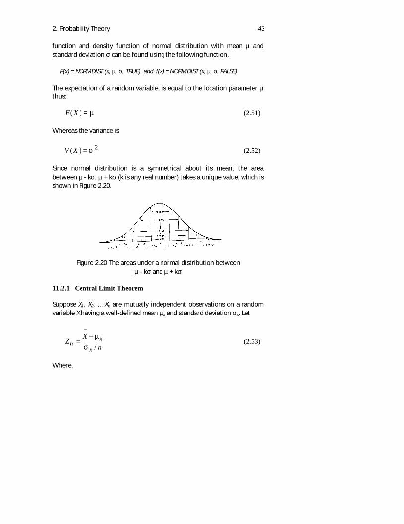
Since normal distribution is a symmetrical about its mean, the areabetween µ - kσ, µ + kσ (k is any real number) takes a unique value, which isshown in Figure 2.20.
Figure 2.20 The areas under a normal distribution betweenµ - kσ and µ + kσ
11.2.1 Central Limit Theorem
Suppose X1, X2, … Xn are mutually independent observations on a randomvariable X having a well-defined mean µx and standard deviation σx. Let
nXZ
x
xn /σ
µ−=
−
(2.53)
Where,
2. Probability Theory 44
∑==
− n
iiX
nX
1
1 (2.54)
and )(zFnz be the cumulative distribution function of the random variable
Zn. Then for all z, - ∞ < z < ∞,
)()(lim zFzF ZZn n
=∞→
(2.55)
where FZ (z) is the cumulative distribution of standard normal distributionN(0,1). The X values have to be from the same distribution but theremarkable feature is that this distribution does not have to be normal, itcan be uniform, exponential, beta, gamma, Weibull or even an unknownone.
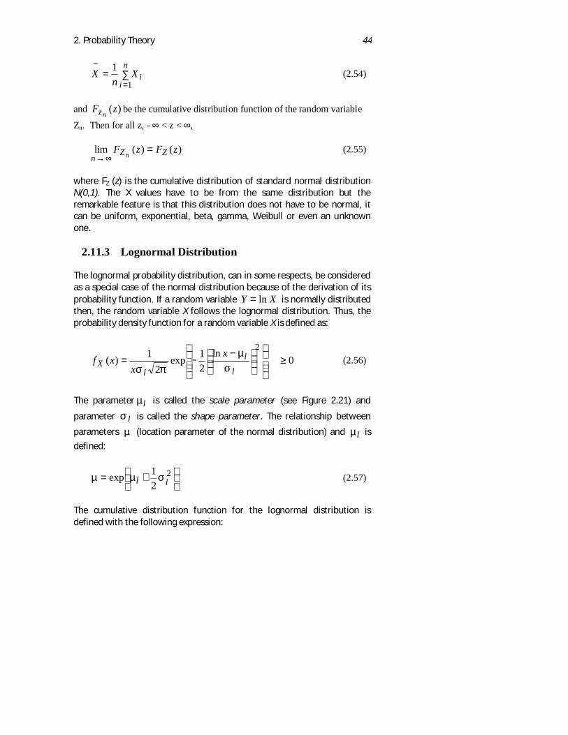
2.11.3 Lognormal Distribution
The lognormal probability distribution, can in some respects, be consideredas a special case of the normal distribution because of the derivation of itsprobability function. If a random variable Y X= ln is normally distributedthen, the random variable X follows the lognormal distribution. Thus, theprobability density function for a random variable X is defined as:
0ln
21exp
21)(
2≥
−−=
l
l
lX
xx
xfσ
µ
πσ(2.56)
The parameter lµ is called the scale parameter (see Figure 2.21) and
parameter lσ is called the shape parameter. The relationship between
parameters µ (location parameter of the normal distribution) and lµ is
defined:
+= 2
21exp ll σµµ (2.57)
The cumulative distribution function for the lognormal distribution isdefined with the following expression:
2. Probability Theory 45
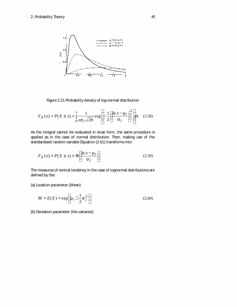
Figure 2.21 Probability density of log-normal distribution
dxx
xxXPxF
x
l
l
lX ∫
−−=≤=
0
2ln21exp
21)()(
σµ
πσ (2.58)
As the integral cannot be evaluated in close form, the same procedure isapplied as in the case of normal distribution. Then, making use of thestandardised random variable Equation (2.61) transforms into:
−Φ=≤=
l
lX
xxXPxFσ
µln)()( (2.59)
The measures of central tendency in the case of lognormal distributions aredefined by the:
(a) Location parameter (Mean)
+== 2
21exp)( llXEM σµ (2.60)
(b) Deviation parameter (the variance)
2. Probability Theory 46
( ) [ ])1exp(2exp)( 22−+= lllXV σσµ (2.61)
2.11.4 Weibull Distribution
This distribution originated from the experimentally observed variations inthe yield strength of Bofors steel, the size distribution of fly ash, fibrestrength of Indian cotton, and the fatigue life of a St-37 steel by the Swedishengineer W.Weibull. As the Weibull distribution has no characteristic shape,such as the normal distribution, it has a very important role in the statisticalanalysis of experimental data. The shape of this distribution is governed byits parameter.
The rule for the probability density function of the Weibull distribution is:
−−
−=
− ββ
ηγ
ηγ
ηβ xxxf exp)(
1(2.65)
where η, β, γ > 0. As the location parameter ν is often set equal to zero, insuch cases:
−
=
− ββ
ηηηβ xxxf exp)(
1(2.66)
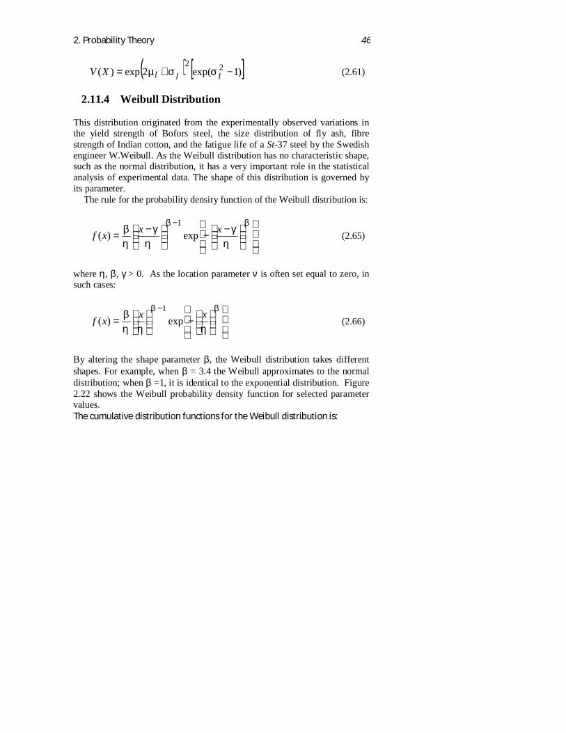
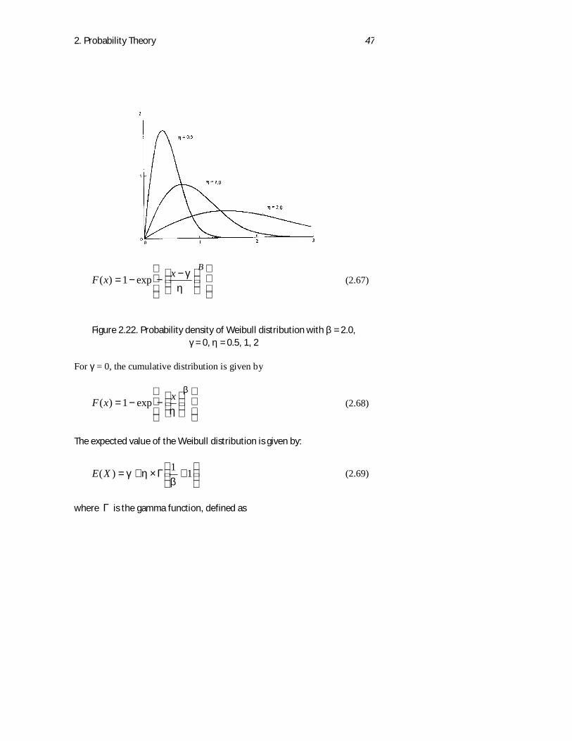
By altering the shape parameter β, the Weibull distribution takes differentshapes. For example, when β = 3.4 the Weibull approximates to the normaldistribution; when β =1, it is identical to the exponential distribution. Figure2.22 shows the Weibull probability density function for selected parametervalues.The cumulative distribution functions for the Weibull distribution is:
2. Probability Theory 47
−−−=
BxxFη
γexp1)( (2.67)
Figure 2.22. Probability density of Weibull distribution with β = 2.0,γ = 0, η = 0.5, 1, 2
For γ = 0, the cumulative distribution is given by
−−=
β
ηxxF exp1)( (2.68)
The expected value of the Weibull distribution is given by:
+Γ×+= 11)(
βηγXE (2.69)
where Γ is the gamma function, defined as
2. Probability Theory 48
dxxen nx 1
0)( −
∞− ×∫=Γ
When n is integer then )!1()( −=Γ nn . For other values, one has to solvethe above integral to the value. Values for this can be found in Gammafunction table given in the appendix. In Microsoft EXCEL, Gamma function,
)(xΓ can be found using the function, EXP[GAMMALN(x)].
The variance of the Weibull distribution is given by:
+Γ−
+Γ=
ββη
1121)()( 22XV (2.70)
3. Reliability Measures 49
Chapter 3
Reliability MeasuresI have seen the future; and it works
Lincoln Steffens
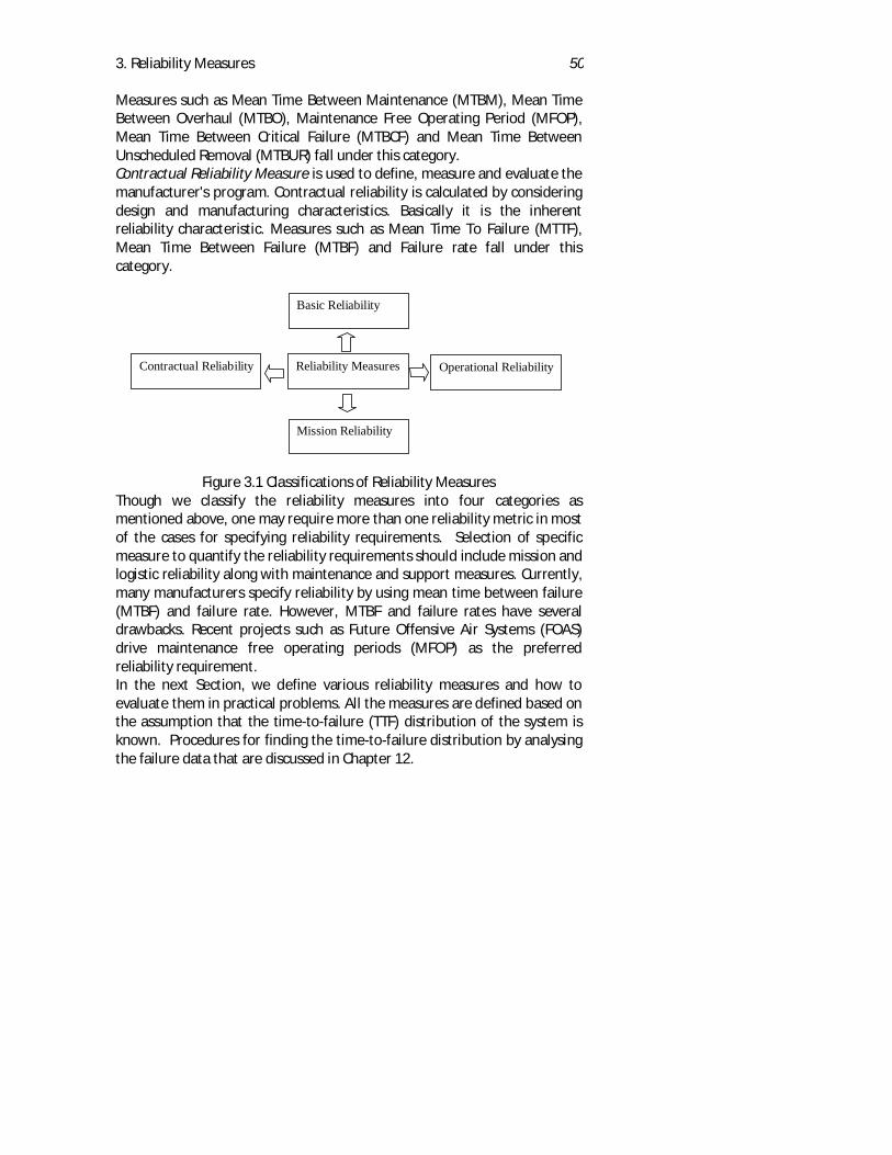
In this chapter we discuss various measures by which hardware andsoftware reliability characteristics can be numerically defined anddescribed. Manufacturers and customers use reliability measure to quantifythe effectiveness of the system. Use of any particular reliability measuredepends on what is expected of the system and what we are tryingmeasure. Several life cycle decision are made using reliability measure asone of the important design parameter. The reliability characteristics ormeasures used to specify reliability must reflect the operationalrequirements of the item. Requirements must be tailored to individual itemconsidering operational environment and mission criticality. In broadersense, the reliability metrics can be classified (Figure 3.1) as: 1. BasicReliability Measures, 2. Mission Reliability Measures, 3. OperationalReliability Measures, and 4. Contractual Reliability Measures.Basic Reliability Measures are used to predict the system's ability to operatewithout maintenance and logistic support. Reliability measures likereliability function and failure function fall under this category.Mission Reliability Measures are used to predict the system's ability tocomplete mission. These measures consider only those failures that causemission failure. Reliability measures such as mission reliability,maintenance free operating period (MFOP), failure free operating period(FFOP), and hazard function fall under this category.Operational Reliability Measures are used to predict the performance of thesystem when operated in a planned environment including the combinedeffect of design, quality, environment, maintenance, support policy, etc.
3. Reliability Measures 50
Measures such as Mean Time Between Maintenance (MTBM), Mean TimeBetween Overhaul (MTBO), Maintenance Free Operating Period (MFOP),Mean Time Between Critical Failure (MTBCF) and Mean Time BetweenUnscheduled Removal (MTBUR) fall under this category.Contractual Reliability Measure is used to define, measure and evaluate themanufacturer's program. Contractual reliability is calculated by consideringdesign and manufacturing characteristics. Basically it is the inherentreliability characteristic. Measures such as Mean Time To Failure (MTTF),Mean Time Between Failure (MTBF) and Failure rate fall under thiscategory.
Figure 3.1 Classifications of Reliability MeasuresThough we classify the reliability measures into four categories asmentioned above, one may require more than one reliability metric in mostof the cases for specifying reliability requirements. Selection of specificmeasure to quantify the reliability requirements should include mission andlogistic reliability along with maintenance and support measures. Currently,many manufacturers specify reliability by using mean time between failure(MTBF) and failure rate. However, MTBF and failure rates have severaldrawbacks. Recent projects such as Future Offensive Air Systems (FOAS)drive maintenance free operating periods (MFOP) as the preferredreliability requirement.In the next Section, we define various reliability measures and how toevaluate them in practical problems. All the measures are defined based onthe assumption that the time-to-failure (TTF) distribution of the system isknown. Procedures for finding the time-to-failure distribution by analysingthe failure data that are discussed in Chapter 12.
Reliability Measures
Basic Reliability
Mission Reliability
Operational ReliabilityContractual Reliability
3. Reliability Measures 51
3.12. FAILURE FUNCTION
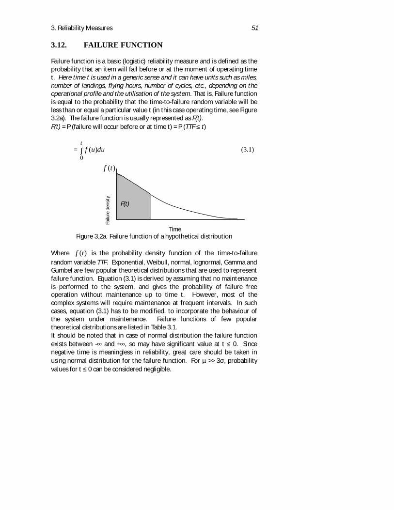
Failure function is a basic (logistic) reliability measure and is defined as theprobability that an item will fail before or at the moment of operating timet. Here time t is used in a generic sense and it can have units such as miles,number of landings, flying hours, number of cycles, etc., depending on theoperational profile and the utilisation of the system. That is, Failure functionis equal to the probability that the time-to-failure random variable will beless than or equal a particular value t (in this case operating time, see Figure3.2a). The failure function is usually represented as F(t).F(t) = P (failure will occur before or at time t) = P (TTF ≤ t)
= duuft∫0
)( (3.1)
Figure 3.2a. Failure function of a hypothetical distribution
Where )(tf is the probability density function of the time-to-failurerandom variable TTF. Exponential, Weibull, normal, lognormal, Gamma andGumbel are few popular theoretical distributions that are used to representfailure function. Equation (3.1) is derived by assuming that no maintenanceis performed to the system, and gives the probability of failure freeoperation without maintenance up to time t. However, most of thecomplex systems will require maintenance at frequent intervals. In suchcases, equation (3.1) has to be modified, to incorporate the behaviour ofthe system under maintenance. Failure functions of few populartheoretical distributions are listed in Table 3.1.It should be noted that in case of normal distribution the failure functionexists between -∞ and +∞, so may have significant value at t ≤ 0. Sincenegative time is meaningless in reliability, great care should be taken inusing normal distribution for the failure function. For µ >> 3σ, probabilityvalues for t ≤ 0 can be considered negligible.
Time
F(t)
f t( )
Failu
re d
ensi
ty
3. Reliability Measures 52
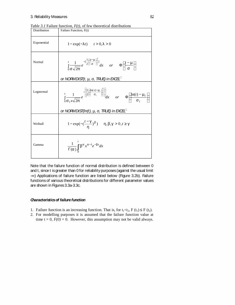
Table 3.1 Failure function, F(t), of few theoretical distributionsDistribution Failure Function, F(t)
Exponential 1 0 0− − > >exp( ) ,λ λt t
Normal∫
−
Φ
−
−tx
tordxe0
]21
[2
21
σµ
πσσ
µ
or NORMDIST(t, µ, σ, TRUE) in EXCEL
Lognormal
∫
−Φ
−−t
l
l
x
l
tordxe
xl
l
0
)ln(21
)ln(2
1
2
σµ
πσ
σµ
or NORMDIST(ln(t), µ, σ, TRUE) in EXCEL
Weibull 1 0− −−
> ≥exp( ( ) ) , , ,t tγη
η β γ γβ
Gamma 1 1
0Γ( )α
βα α βx e dxxt
− −∫
Note that the failure function of normal distribution is defined between 0and t, since t is greater than 0 for reliability purposes (against the usual limit-∞) Applications of failure function are listed below (Figure 3.2b). Failurefunctions of various theoretical distributions for different parameter valuesare shown in Figures 3.3a-3.3c.
Characteristics of failure function
1. Failure function is an increasing function. That is, for t1<t2, F (t1) ≤ F (t2).2. For modelling purposes it is assumed that the failure function value at
time t = 0, F(0) = 0. However, this assumption may not be valid always.
3. Reliability Measures 53
For example, systems can be dead on arrival. The value of failurefunction increases as the time increases and for t = ∞, F(∞) = 1.
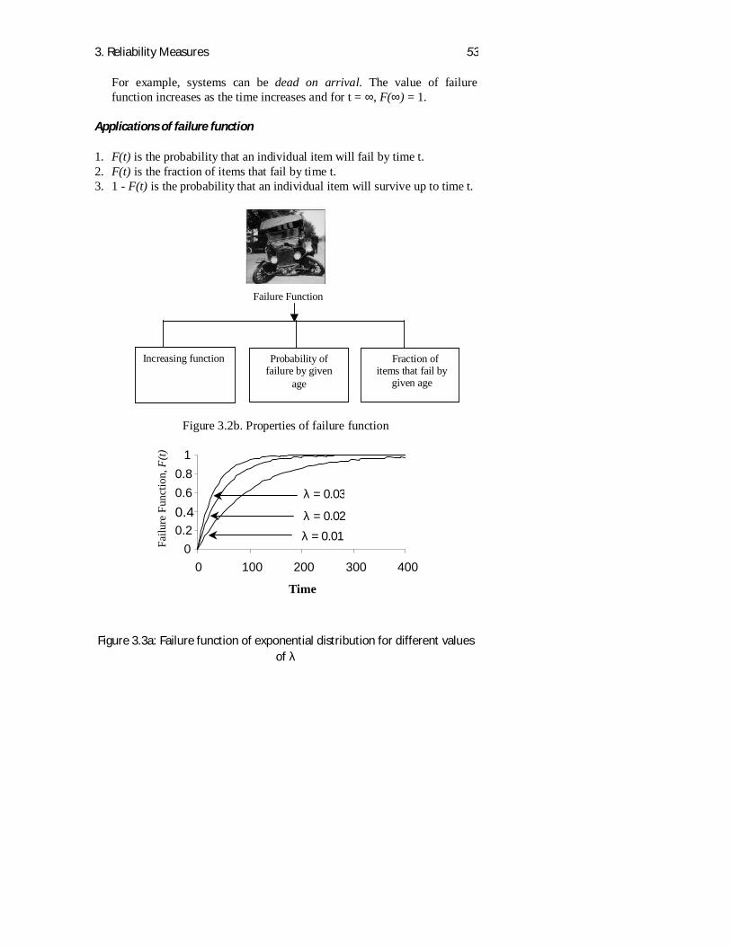
Applications of failure function
1. F(t) is the probability that an individual item will fail by time t.2. F(t) is the fraction of items that fail by time t.3. 1 - F(t) is the probability that an individual item will survive up to time t.
Figure 3.2b. Properties of failure function
Figure 3.3a: Failure function of exponential distribution for different valuesof λ
Failure Function
Increasing function Probability offailure by given
age
Fraction ofitems that fail by
given age
00.20.40.60.8
1
0 100 200 300 400
Time
λ = 0.03
Failu
re F
unct
ion,
F(t)
λ = 0.02
λ = 0.01
3. Reliability Measures 54
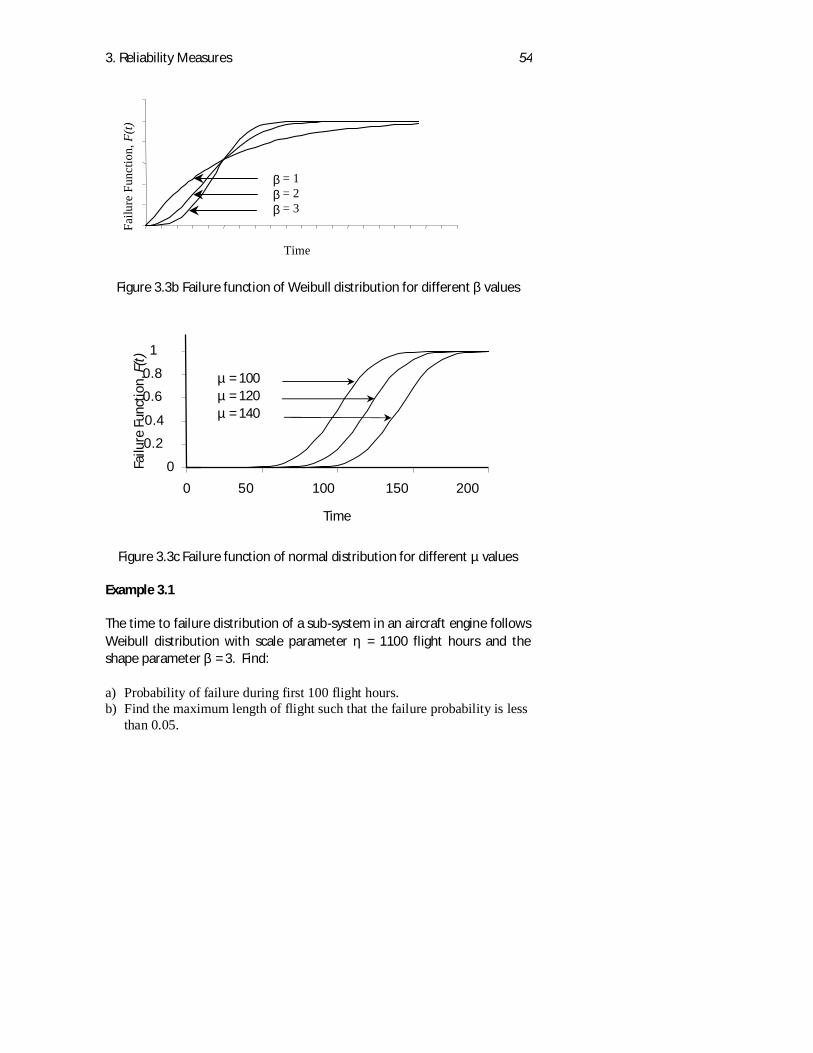
Figure 3.3b Failure function of Weibull distribution for different β values
Figure 3.3c Failure function of normal distribution for different µ values
Example 3.1
The time to failure distribution of a sub-system in an aircraft engine followsWeibull distribution with scale parameter η = 1100 flight hours and theshape parameter β = 3. Find:
a) Probability of failure during first 100 flight hours.b) Find the maximum length of flight such that the failure probability is less
than 0.05.
0
0.2
0.4
0.6
0.8
1
0 50 100 150 200
Time
µ = 100µ = 120µ = 140
Failu
re F
unct
ion,
F(t)
Failu
re F
unct
ion,
F(t)
β = 1β = 2β = 3
Time
3. Reliability Measures 55
SOLUTION:
a) The failure function for Weibull distribution is given by:
F t t( ) exp( ( ) )= − −−1 γη
β
It is given that: t = 100 flight hours, η = 1100 flight hours, β = 3 and γ = 0.
Probability of failure within first 100 hours is given by:
F ( ) exp( ( ) ) .100 1 100 01100
0 000753= − − − =
b) If t is the maximum length of flight such that the failure probability is lessthan 0.05, we have
3/13
3
3
)]95.0ln([110095.0ln)1100
(
95.0))1100
(exp(
05.0))1100
0(exp(1)(
−×=⇒−>=
>−=
<−
−−=
tt
t
ttF
Now solving for t, we get t = 408.70 flight hours. The maximum length offlight such that the failure probability is less than 0.05 is 408.70 flight hours.
Example 3.2
The time to failure distribution of a Radar Warning Receiver (RWR) systemin a fighter aircraft follows Weibull distribution with scale parameter 1200flight hours and shape parameter 3. The time to failure distribution of thesame RWR in a helicopter follows exponential distribution with scaleparameter 0.001. Compare the failure function of the RWR in the fighteraircraft and the helicopter. If the supplier gives a warranty for 750 flighthours, calculate the risk involved with respect to fighter aircraft and thehelicopter. (Although we have a same system, the operating conditionshave significant impact on the failure function. In this case, RWR inhelicopter is subject to more vibrations compared to aircraft).
3. Reliability Measures 56
SOLUTION:
The failure function of RWR on the fighter aircraft is given by:
F t t( ) exp( ( ) )= − −11200
3
The failure function of RWR on the helicopter is given by:
F t t( ) exp( ( . ))= − − ×1 0 001
Figure 3.4 depicts the failure function of RWR in fighter aircraft and thehelicopter.
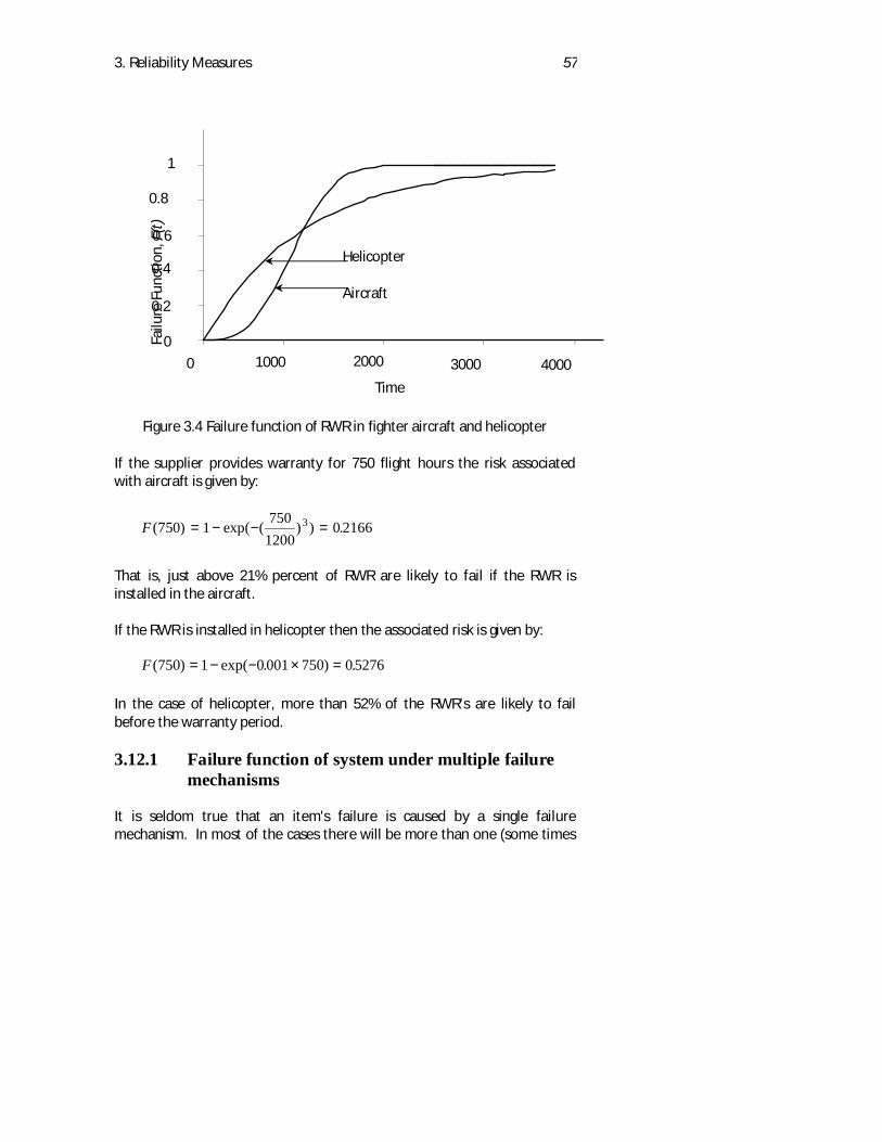
3. Reliability Measures 57
Figure 3.4 Failure function of RWR in fighter aircraft and helicopter
If the supplier provides warranty for 750 flight hours the risk associatedwith aircraft is given by:
F ( ) exp( ( ) ) .750 1 7501200
0 21663= − − =
That is, just above 21% percent of RWR are likely to fail if the RWR isinstalled in the aircraft.
If the RWR is installed in helicopter then the associated risk is given by:
F ( ) exp( . ) .750 1 0 001 750 05276= − − × =
In the case of helicopter, more than 52% of the RWR’s are likely to failbefore the warranty period.
3.12.1 Failure function of system under multiple failuremechanisms
It is seldom true that an item's failure is caused by a single failuremechanism. In most of the cases there will be more than one (some times
Failu
re F
unct
ion,
F(t)
Helicopter
Aircraft
Time
0 1000 2000 3000 4000
0.2
0.4
0.6
0.8
1
0
3. Reliability Measures 58
hundreds) mechanism that causes the failure of an item. The expression(3.1) is more appropriate when the failure is caused by a single failuremechanism. However, most of the practical systems fail due to differentcauses or different failure mechanisms. Assume that the system failure isdue to two different failure mechanisms. Let f1(t) and f2(t) be the probabilitydensity function of the system due to failure mechanism 1 and 2respectively. Now the probability density function of the time-to-failure ofthe system caused by either of the failure mechanisms:
)](1)[()](1)[()( 1221 tFtftFtftf −+−=
where, F1(t) and F2(t) the are failure function for failure mechanism 1 and 2respectively. The failure function of the item under two different failuremechanism is given by:
∫ −+−=t
dxxFxfxFxftF0
1221 )]}(1)[()](1)[({)( (3.2)
Example 3.3
Failure of an item is caused by two different failure mechanisms (say failuremechanism A and B). The time-to-failure distribution of the item due tofailure mechanism A can be represented by exponential distribution withparameter λA = 0.002 hours. The time-to-failure distribution of the item dueto failure mechanism B can be represented by exponential distribution withparameter λB = 0.005 hours. Find the probability that the item will failbefore 500 hours of operation.
SOLUTION:Assume that fA(t) and fB(t) represent probability density function of thetime-to-failure random variable due to failure mechanism A and Brespectively. Thus,
f t t F t tf t t F t t
A A A A A
B B B B B
( ) exp( ) , ( ) exp( )( ) exp( ) , ( ) exp( )
= − − = −= − − = −
λ λ λλ λ λ
11
Now the failure function of the item is given by:
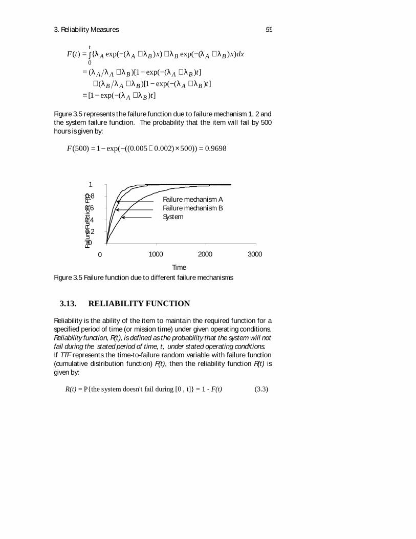
3. Reliability Measures 59
])(exp(1[])(exp(1)[(
])(exp(1)[(
))(exp())(exp({)(0
tt
t
dxxxtF
BA
BABAB
BABAA
BAt
BBAA
λλλλλλλ
λλλλλ
λλλλλλ
+−−=+−−++
+−−+=
+∫ −++−=
Figure 3.5 represents the failure function due to failure mechanism 1, 2 andthe system failure function. The probability that the item will fail by 500hours is given by:
9698.0))500)002.0005.0((exp(1)500( =×+−−=F
Figure 3.5 Failure function due to different failure mechanisms
3.13. RELIABILITY FUNCTION
Reliability is the ability of the item to maintain the required function for aspecified period of time (or mission time) under given operating conditions.Reliability function, R(t), is defined as the probability that the system will notfail during the stated period of time, t, under stated operating conditions.If TTF represents the time-to-failure random variable with failure function(cumulative distribution function) F(t), then the reliability function R(t) isgiven by:
R(t) = P{the system doesn't fail during [0 , t]} = 1 - F(t) (3.3)
0
0.2
0.4
0.6
0.8
1
0 1000 2000 3000
Time
Failu
re F
unct
ion,
F(t) Failure mechanism A
Failure mechanism BSystem
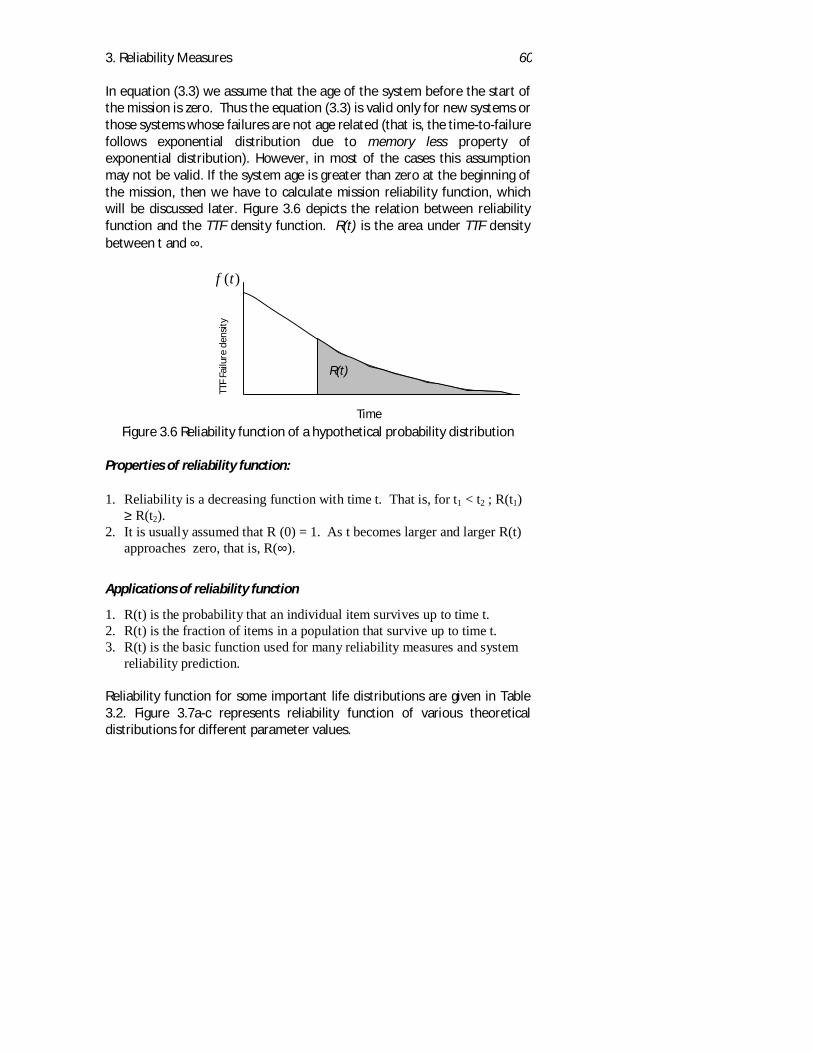
3. Reliability Measures 60
In equation (3.3) we assume that the age of the system before the start ofthe mission is zero. Thus the equation (3.3) is valid only for new systems orthose systems whose failures are not age related (that is, the time-to-failurefollows exponential distribution due to memory less property ofexponential distribution). However, in most of the cases this assumptionmay not be valid. If the system age is greater than zero at the beginning ofthe mission, then we have to calculate mission reliability function, whichwill be discussed later. Figure 3.6 depicts the relation between reliabilityfunction and the TTF density function. R(t) is the area under TTF densitybetween t and ∞.
Figure 3.6 Reliability function of a hypothetical probability distribution
Properties of reliability function:
1. Reliability is a decreasing function with time t. That is, for t1 < t2 ; R(t1)≥ R(t2).
2. It is usually assumed that R (0) = 1. As t becomes larger and larger R(t)approaches zero, that is, R(∞).
Applications of reliability function
1. R(t) is the probability that an individual item survives up to time t.2. R(t) is the fraction of items in a population that survive up to time t.3. R(t) is the basic function used for many reliability measures and system
reliability prediction.
Reliability function for some important life distributions are given in Table3.2. Figure 3.7a-c represents reliability function of various theoreticaldistributions for different parameter values.
Time
f t( )
TTF
Failu
re d
ensi
ty
R(t)
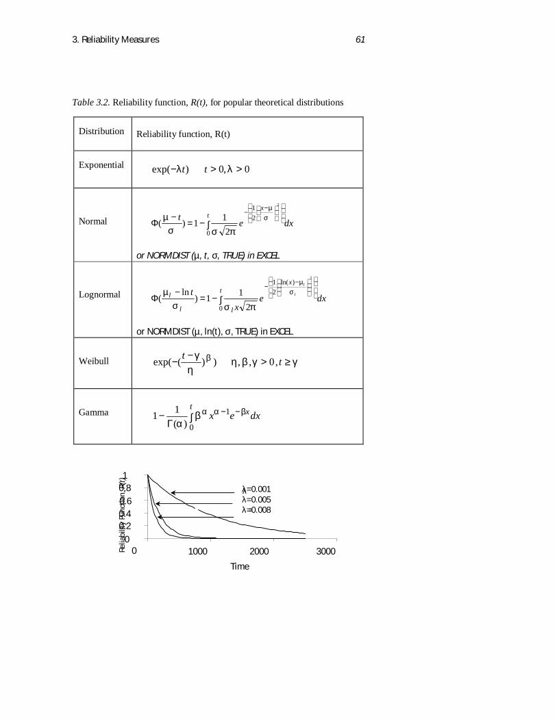
3. Reliability Measures 61
Table 3.2. Reliability function, R(t), for popular theoretical distributions
Distribution Reliability function, R(t)
Exponential 0,0)exp( >>− λλ tt
Normal dxet tx
∫−=−
Φ
−
−
0
21 2
211)( σ
µ
πσσµ
or NORMDIST (µ, t, σ, TRUE) in EXCEL
Lognormal dxex
t tx
ll
l l
l
∫−=−
Φ
−−
0
)ln(21
2
211)
ln(
σµ
πσσµ
or NORMDIST (µ, ln(t), σ, TRUE) in EXCEL
Weibull γγβηη
γ β ≥>−
− tt ,0,,))(exp(
Gamma ∫Γ
− −−t xdxex0
1)(
11 βααβα
00.20.40.60.81
0 1000 2000 3000
Time
λλ=0.001λ=0.005λ=0.008 =
Relia
bilit
y Fu
nctio
n,R(
t)

3. Reliability Measures 62
Figure 3.7 a. Reliability function of exponential distribution for differentvalues of λ
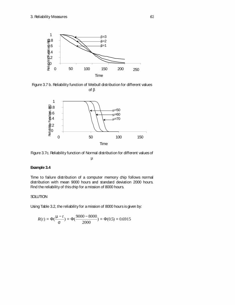
3. Reliability Measures 63
Figure 3.7 b. Reliability function of Weibull distribution for different valuesof β
Figure 3.7c. Reliability function of Normal distribution for different values ofµ
Example 3.4
Time to failure distribution of a computer memory chip follows normaldistribution with mean 9000 hours and standard deviation 2000 hours.Find the reliability of this chip for a mission of 8000 hours.
SOLUTION
Using Table 3.2, the reliability for a mission of 8000 hours is given by:
R t t( ) ( ) ( ) ( . ) .=−
=−
= =Φ Φ Φµ
σ9000 8000
20000 5 0 6915
00.2
0.40.6
0.8
1
0 50 100 150
Time
Relia
bilit
y Fu
nctio
n,R(
t)
µ=50µ=60µ=70
0
0.20.4
0.60.8
1
0 50 100 150 200 250
Time
Relia
bilit
y Fu
nctio
n,R(
t)
β=3β=2β=1
3. Reliability Measures 64
Example 3.5
The time to failure distribution of a steam turbo generator can berepresented using Weibull distribution with η = 500 hours and β = 2.1. Findthe reliability of the generator for 600 hours of operation.
SOLUTION:
Again using Table 3.2, reliability of the generator for 600 hours ofoperations is given by:
R t( ) exp( ( / ) ) .= − =600 500 0 23072.1
3.13.1 Reliability function for items under multiple failuremechanisms
Assume that the failure of the item is caused due to two different failuremechanisms. Let f1(t) and f2(t) be the probability density function of thetime-to-failure random variable due to failure mechanism 1 and 2respectively. The probability density function of the time-to-failure of theitem is given by caused by either of the failure mechanisms:
)](1[)()](1)[()( 1221 tFtftFtftf −⋅+−=
Where F1(t) and F2(t) are failure function for failure mechanism 1 and 2respectively. The Reliability function of the item under two different failuremechanism is given by:
∫ −+−−=−=t
dxxFxfxFxftFtR0
1221 )]}(1)[()](1)[({1)(1)( (3.4)
The above result can be extended to obtain expression for reliabilityfunction due to more than two failure mechanisms.
Example 3.6
For the example 3.3, find the reliability of the item for 200 hours.
SOLUTION:
3. Reliability Measures 65
Using the expression for failure function obtained in example 3.3, thereliability function can be written as:
2465.0)200)005.0002.0(exp()200())(exp()(
=×+−=×+−=
RttR BA λλ
3.13.2 Mission Reliability Function
In many practical situations, one might be interested in finding theprobability of completing a mission successfully. Success probability ofhitting an enemy target and returning to the base is an example wheremission reliability function can be used. The main difference betweenreliability function and the mission reliability function is that, in missionreliability we recognise the age of the system before the mission. Missionreliability is defined, as the probability that the system aged tb is able tocomplete mission duration of tm successfully. We assume that nomaintenance is performed during the mission. The expression for missionreliability MR (tb , tm) is given by
)()(
),(b
mbmb tR
ttRttMR += (3.5)
where, tb is the age of the item at the beginning of the mission and tm is themission period. If the time to failure distribution is exponential, then thefollowing relation is valid.
)(),( mmb tRttMR =
Application of mission reliability function
1. Mission reliability, MR(ta, tm) gives the probability that an individualitem aged ta will complete a mission duration of tm hours without anyneed for maintenance.
2. Mission reliability is the appropriate basic reliability measure for ageingitems or items whose time-to-failure distribution is other thenexponential.
Example 3.7
3. Reliability Measures 66
Time-to-failure distribution of the gearbox within an armoured vehicle canbe modelled using Weibull distribution with scale parameter η = 2400 milesand shape parameter β = 1.25. Find the probability that that gearbox willnot fail during a mission time of 200 miles. Assuming that the age of thegearbox is 1500 miles.
SOLUTION:
Given, tb = 1500 miles and tm = 200 miles
)1500()1700(
)()(
),(RR
tRttRttMR
b
bmmb =
+=
5221.0))24001700(exp()1700( 25.1 =−=R
5736.0))24001500(exp()1500( 25.1 =−=R
9102.05736.05221.0
)1500()1700()200,1500( ===
RRMR
That is, the gearbox aged 1500 miles has approximately 91% chance ofsurviving a mission of 200 miles.
3.14. DESPATCH RELIABILITY
Despatch reliability (DR) is one of popular reliability metrics used bycommercial airlines around the world. Despatch reliability is defined as thepercentage of revenue departures that do not occur in a delay orcancellation due to technical problems. For most airlines, the delay meansthat the aircraft is delayed more than 15 minutes. Technical delays occurcan be caused due to some unscheduled maintenance. Airlines frequentlyseek DR guarantees where the aircraft manufactures face penalties if DRlevels are not achieved. For commercial airlines despatch reliability is animportant economic factor, it is estimated that delay cost per minute for
3. Reliability Measures 67
large jets can be as high as 1000 US dollars. The expression for despatchreliability is given by:
%100100
100(%) 15 ×
−−=
NCNDDR (3.6)
Where,
ND15 = Number of delays with more than 15 minutes delay
NC = the number of cancellations
Equation (3.6) is applied only to technical delays. DR is a function ofequipment reliability, system and component maintainability, and overalllogistic support.
3.15. HAZARD FUNCTION (HAZARD RATE ORINSTANTANEOUS FAILURE RATE)
Hazard function (or hazard rate) is used as a parameter for comparison oftwo different designs in reliability theory. Hazard function is the indicator ofthe effect of ageing on the reliability of the system. It quantifies the risk offailure as the age of the system increases. Mathematically, it represents theconditional probability of failure in an interval t to t + δt given that thesystem survives up to t, divided by δt, as δt tends to zero, that is,
)()()(lim
)()()(.1lim)(
00 ttRttRtR
tRtFttF
tth
tt δδδ
δ δδ
+−=
−+=
→→ (3.7)
Note that hazard function, h(t), is not a probability, it is the limiting value ofthe probability. However, h(t)δt, represents the probability that the itemwill fail between ages t and t+δt as δt →0. The above expression can besimplified so that
h t f tR t
( ) ( )( )
= (3.8)
3. Reliability Measures 68
Thus, the hazard function is the ratio of the probability density function tothe reliability function. Integrating both sides of the above equation, weget:
h x dx f xR x
dx
R xR x
dx R t
t t
t
( ) ( )( )
' ( )( )
ln ( )
0 0
0
∫ = ∫
= −∫ = −
Thus reliability can be written as:
R t h x dxt
( ) exp ( )= −
∫
0(3.9)
From equation (3.9), it immediately follows that:
f t h t h x dxt
( ) ( ) exp( ( )= −∫0
(3.10)
The expression (3.10), which relates reliability and hazard function, is validfor all types of time to failure distribution. Hazard function shows how therisk of the item in use changes over time (hence also called risk rate). Thehazard functions of some important theoretical distributions are given inTable 3.3.
Characteristics of hazard function
1. Hazard function can be increasing, decreasing or constant.2. Hazard function is not a probability and hence can be greater than 1.
Table 3.3. Hazard function, h(t), of few theoretical distributions
Distribution Hazard function, h(t)
Exponential λ
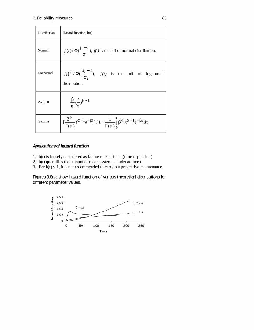
3. Reliability Measures 69
Distribution Hazard function, h(t)
Normal ),(/)(σ
µ ttf −Φ f(t) is the pdf of normal distribution.
Lognormal ),(/)(l
ll
ttf
σµ −
Φ fl(t) is the pdf of lognormal
distribution.
Weibull 1)( −βηη
β t
Gamma [( )
] /( )
βα α
βα
α β α α βΓ Γ
t e x e dxt xt− − − −− ∫1 1
01 1
Applications of hazard function
1. h(t) is loosely considered as failure rate at time t (time-dependent)2. h(t) quantifies the amount of risk a system is under at time t.3. For h(t) ≤ 1, it is not recommended to carry out preventive maintenance.
Figures 3.8a-c show hazard function of various theoretical distributions fordifferent parameter values.
0
0.02
0.04
0.06
0.08
0 50 100 150 200 250
Time
haza
rd fu
nctio
n
β = 2.4β = 0.8
β = 1.6
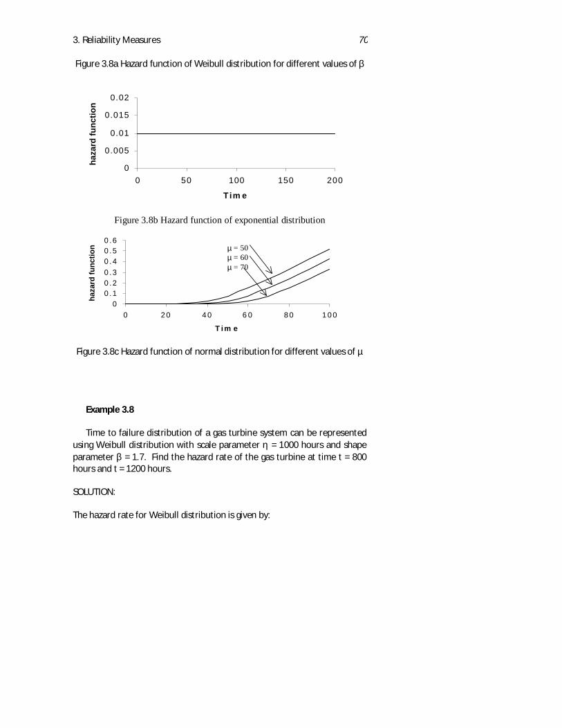
3. Reliability Measures 70
Figure 3.8a Hazard function of Weibull distribution for different values of β
Figure 3.8b Hazard function of exponential distribution
Figure 3.8c Hazard function of normal distribution for different values of µ
Example 3.8
Time to failure distribution of a gas turbine system can be representedusing Weibull distribution with scale parameter η = 1000 hours and shapeparameter β = 1.7. Find the hazard rate of the gas turbine at time t = 800hours and t = 1200 hours.
SOLUTION:
The hazard rate for Weibull distribution is given by:
0
0.005
0.01
0.015
0.02
0 50 100 150 200
Tim e
haza
rd fu
nctio
n
00 .10 .20 .30 .40 .50 .6
0 2 0 4 0 6 0 8 0 1 0 0
T im e
haza
rd fu
nctio
n µ = 50µ = 60µ = 70
3. Reliability Measures 71
h t t( ) ( )= −βη η
β 1
h(800 ) = 171000
8001000
0 001450 7. ( ) .. =
h(1200 ) = 171000
12001000
0 00190 7. ( ) .. =
3.15.1 Cumulative hazard function
Cumulative hazard function represents the cumulative hazard or risk of theitem during the interval [0,t]. Cumulative hazard function, H(t), is given by:
H t h x dxt
( ) ( )= ∫0
(3.11)
Reliability of an item can be conveniently written using cumulative hazardas:
R t e H t( ) ( )= − (3.12)
3.15.2 Cumulative hazard function and the expectednumber of failures
Consider an item, which upon failure is subject to minimal repair. That is,the hazard rate after repair is same as the hazard rate just before failure. IfN(t) is the total number of failures by time t, then M(t) = E [N(t)] is theexpected number of failures by time t. It can be shown that under theassumption that the item receives minimal repair* (‘as-bad -as-old’) aftereach failure, then
E[N(t)] = ∫=t
dxxhtM0
)()( (3.13)
* Mathematically minimal repair or as bad as old means that the hazard rate of the itemafter repair will be same as the hazard rate just prior to failure.
3. Reliability Measures 72
The above expression can be used to model differentmaintenance/replacement policies. In case of exponential and Weibull timeto failure distributions we get the following simple expressions for theexpected number of failures of an item subject to minimal repair.
Exponential time to failure distribution
For exponential distribution, the expected number of failures is given by
E[N(t)] = h x dx dx tt t
( )0 0∫ = ∫ =λ λ (3.14)
Weibull time to failure distribution
E[N(t)] = h x dx x dx tt t
( ) ( ) ( )0
1
0∫ ∫= =−β
η η ηβ β (3.15)
Example 3.9An item is subject to minimal repair whenever it failed. If the time to failureof the item follows Weibull distribution with η = 500 and β = 2. Find: 1. Thenumber of times the item is expected to fail by 1500 hours, and 2. The costof the item is $ 200. If the cost of minimal repair is $ 100 per each repair, isit advisable to repair or replace the item upon failure.
SOLUTION:
1. The expected number of failures is given by:
E[N(t)] = [ ] [ ]tη
β = = =1500500
3 92 2
2. Using the above result the cost associated with repair, Crepair (t) = 9 × 100= $ 900.If the item is replaced, then the expected number of failures is given by therenewal function, M(t) [refer chapter 4], where
3. Reliability Measures 73
M t F ti
i
( ) ( )==
∞
∑1
For the above case, the value of M(t) < 4 (The actual calculation of theabove function will be discussed in Chapter 4). Thus the cost due toreplacement will be less than 4 × 200 = $ 800. Thus, it is better to replacethe item upon failure rather using minimal repair.
3.15.3 Typical Forms of Hazard Function
In practice, hazard function can have different shapes. Figure 3.9 showsmost general forms of hazard function. Recent research in the field ofreliability centred maintenance (RCM) shows that the hazard rate mostlyfollows six different patterns. Depending on the equipment and its failuremechanism, one can say that the hazard function may follow any one ofthese six patterns. However, one should not blindly assume that hazardrate of any item will follow any one of these six patterns. These are onlypossible cases based on some data.Pattern A is called the bathtub curve and consist of three distinct phases. Itstarts with early failure region (known as burn-in or infant mortality)characterised by decreasing hazard function. Early failure region is followedby constant or gradually increasing region (called useful life). The constantor gradually increasing region is followed by wear out region characterisedby increasing hazard function. The reason for such as shape is that theearly decreasing hazard rate results from manufacturing defects. Earlyoperation will remove these items from a population of like items. Theremaining items have a constant hazard for some extended period of timeduring which the failure cause is not readily apparent. Finally those itemsremaining reach a wear-out stage with an increasing hazard rate. Onewould expect bathtub curve at the system level and not at the part orcomponent level (unless the component has many failure modes whichhave different TTF distribution). It was believed that bathtub curverepresents the most general form of the hazard function. However, therecent research shows that in most of the cases hazard function do notfollow this pattern.Pattern B starts with high infant mortality and then follows a constant orvery slowly increasing hazard function. Pattern C starts with a constant orslowly increasing failure probability followed by wear out (sharplyincreasing) hazard function. Pattern D shows constant hazard throughoutthe file. Pattern E represents a slowly increasing hazard without any sign of
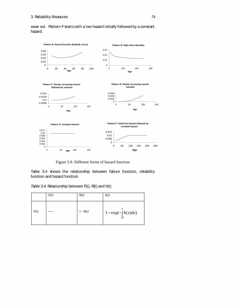
3. Reliability Measures 74
wear out. Pattern F starts with a low hazard initially followed by a constanthazard.
Figure 3.9. Different forms of hazard function
Table 3.4 shows the relationship between failure function, reliabilityfunction and hazard function.
Table 3.4. Relationship between F(t), R(t) and h(t)
F(t) R(t) h(t)
F(t) ----- 1 - R(t) ∫−−t
dxxh0
))(exp(1
Pattern A: Hazard function (bathtub curve)
00.010.020.030.04
0 20 40 60 80 100Age
Pattern B: High infant Mortality
0
0.01
0.02
0.03
0 100 200 300Age
Pattern D: Constant Hazard
00.0020.0040.0060.008
0.010.012
0 50 100 150Age
Pattern E: Slowly increasing hazardfunction
00.00020.00040.0006
0 50 100 150
Age
Pattern C: Slowly increasing hazardfollowed by wearout
0.009950.01
0.010050.0101
0 50 100 150
Age
Pattern F: Initial low hazard followed byconstant hazard
00.0050.01
0.015
0 50 100 150 200 250Age
3. Reliability Measures 75
F(t) R(t) h(t)
R(t) 1 - F(t) ------ ∫−t
dxxh0
)(exp(
h(t) )](1[)(' tRtF − )()(' tRtR− -------
3.15.4 Failure rate
Whenever the hazard function is constant, we call it as failure rate. That is,failure rate is a special case of hazard function (which is time dependentfailure rate). Failure rate is one of the most widely used contractualreliability measures in the defence and aerospace industry. By definition, itis appropriate to use failure rate only when the time-to-failure distributionis exponential. Also, failure rate can be used only for a non-repairablesystem. Many defence standards such as MIL-HDBK-217 and British DEF-STAN 00-40 recommend the following equation for estimating the failurerate.
sampletheoftimeoperatingCumulativesampleainfailuresofnumberTotal
rateFailure = (3.16)
Care should be taken in using the above equation, for good estimation onehas to observe the system failure for a sufficiently large operating period.
Applications of failure rate
1. Failure rate represents the number of failures per unit time.2. If the failure rate is λ, then the expected number of items that fail in [0,t]
is λt.3. Failure rate is one of the popular contractual reliability measures among
many industries including aerospace and defence.
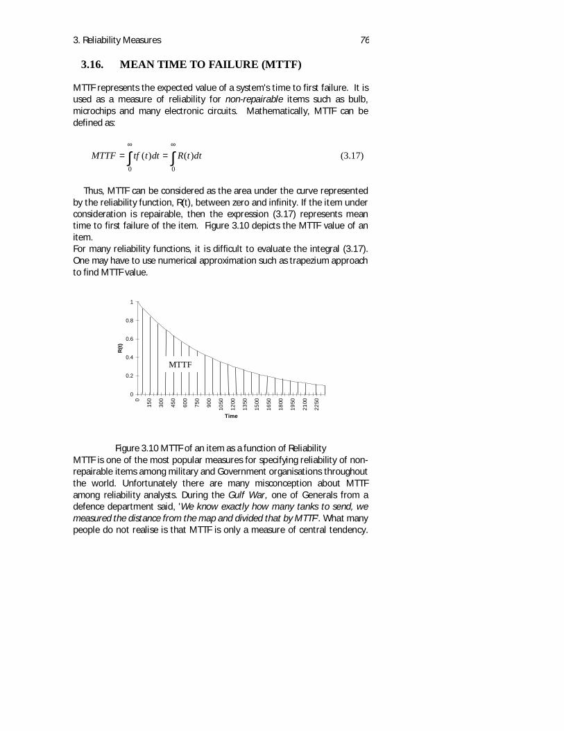
3. Reliability Measures 76
3.16. MEAN TIME TO FAILURE (MTTF)
MTTF represents the expected value of a system's time to first failure. It isused as a measure of reliability for non-repairable items such as bulb,microchips and many electronic circuits. Mathematically, MTTF can bedefined as:
MTTF tf t dt R t dt= =∞ ∞
∫ ∫( ) ( )0 0
(3.17)
Thus, MTTF can be considered as the area under the curve representedby the reliability function, R(t), between zero and infinity. If the item underconsideration is repairable, then the expression (3.17) represents meantime to first failure of the item. Figure 3.10 depicts the MTTF value of anitem.For many reliability functions, it is difficult to evaluate the integral (3.17).One may have to use numerical approximation such as trapezium approachto find MTTF value.
Figure 3.10 MTTF of an item as a function of ReliabilityMTTF is one of the most popular measures for specifying reliability of non-repairable items among military and Government organisations throughoutthe world. Unfortunately there are many misconception about MTTFamong reliability analysts. During the Gulf War, one of Generals from adefence department said, 'We know exactly how many tanks to send, wemeasured the distance from the map and divided that by MTTF'. What manypeople do not realise is that MTTF is only a measure of central tendency.
0
0.2
0.4
0.6
0.8
1
0
150
300
450
600
750
900
1050
1200
1350
1500
1650
1800
1950
2100
2250
Time
R(t)
MTTF
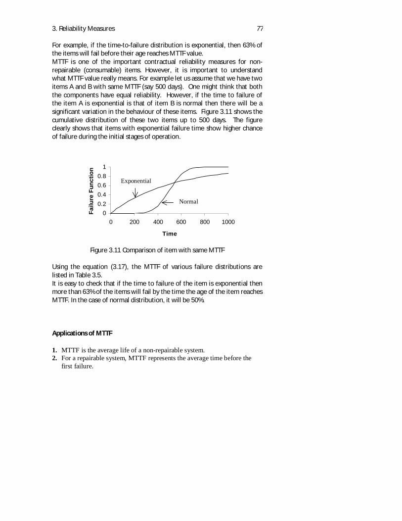
3. Reliability Measures 77
For example, if the time-to-failure distribution is exponential, then 63% ofthe items will fail before their age reaches MTTF value.MTTF is one of the important contractual reliability measures for non-repairable (consumable) items. However, it is important to understandwhat MTTF value really means. For example let us assume that we have twoitems A and B with same MTTF (say 500 days). One might think that boththe components have equal reliability. However, if the time to failure ofthe item A is exponential is that of item B is normal then there will be asignificant variation in the behaviour of these items. Figure 3.11 shows thecumulative distribution of these two items up to 500 days. The figureclearly shows that items with exponential failure time show higher chanceof failure during the initial stages of operation.
Figure 3.11 Comparison of item with same MTTF
Using the equation (3.17), the MTTF of various failure distributions arelisted in Table 3.5.It is easy to check that if the time to failure of the item is exponential thenmore than 63% of the items will fail by the time the age of the item reachesMTTF. In the case of normal distribution, it will be 50%.
Applications of MTTF
1. MTTF is the average life of a non-repairable system.2. For a repairable system, MTTF represents the average time before the
first failure.
00.20.40.60.8
1
0 200 400 600 800 1000
Time
Failu
re F
unct
ion
Normal
Exponential
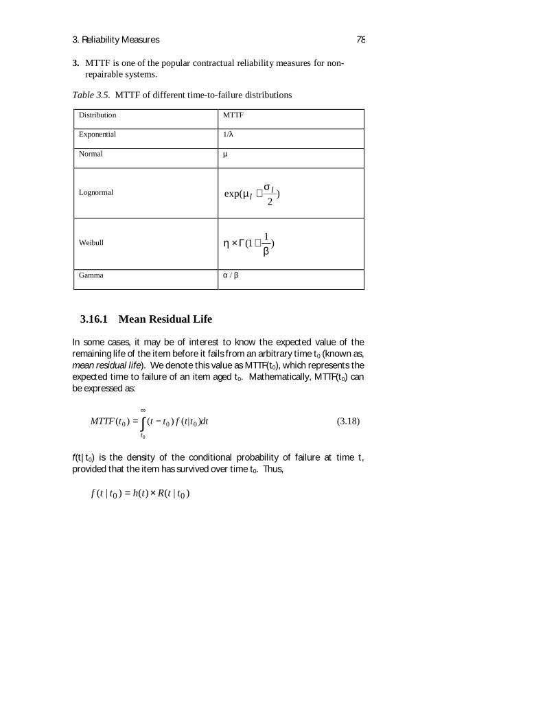
3. Reliability Measures 78
3. MTTF is one of the popular contractual reliability measures for non-repairable systems.
Table 3.5. MTTF of different time-to-failure distributions
Distribution MTTF
Exponential 1/λ
Normal µ
Lognormal )2
exp( ll
σµ +
Weibull )11(β
η +Γ×
Gamma α / β
3.16.1 Mean Residual Life
In some cases, it may be of interest to know the expected value of theremaining life of the item before it fails from an arbitrary time t0 (known as,mean residual life). We denote this value as MTTF(t0), which represents theexpected time to failure of an item aged t0. Mathematically, MTTF(t0) canbe expressed as:
MTTF t t t f t t dtt
( ) ( ) ( | )0 0 0
0
= −∞
∫ (3.18)
f(t|t0) is the density of the conditional probability of failure at time t,provided that the item has survived over time t0. Thus,
)|()()|( 00 ttRthttf ×=
3. Reliability Measures 79
where, R(t|t0), is the conditional probability that the item survives up totime t, given that it has survived up to time t0. Now, the above expressioncan be written as:
)()()()|(
00 tR
tRthttf ×=
The expression for MTTF(t0) can be written as:
MTTF t t t h t R tR t
dtt
( ) ( ) ( ) ( )( )0 0
00
= −∞
∫ (3.19)
substituting for h(t) in the above equation, we have
MTTF t t t f tR t
dtR t
t t f t dtt t
( ) ( ) ( )( ) ( )
( ) ( )00
0 00
0 0
1=−
= −∞ ∞
∫ ∫
The above equation can be written as (using integration by parts):
MTTF t
R t dt
R tt( )
( )
( )00
0=
∞
∫(3.20)
The concept of mean residual life can be successfully applied for planningmaintenance and inspection activities.
Example 3.10
Companies A and B manufacture car tyres. Both the companies claim thatthe MTTF of their car tyre is 2000 miles. After analysing the field failuredata of these two tyres it was found that the time to failure distribution ofA is exponential with λ = 0.0005 and the time to failure distribution of B isnormal with µ = 2000 miles and σ = 200 miles. If the maintenance policy ofthe Exeter city car rentals is to replace the tyres as soon as it reaches 2000miles which tyre they should buy:
SOLUTION:
3. Reliability Measures 80
Reliability of the car tyre produced by company A for 2000 miles, RA(2000),is given by:
3678.0)20000005.0exp()2000( =×−=AR
Reliability of the car tyre produced by company B for 2000 miles, RB(2000),is given by:
RB ( ) ( ) ( ) ( ) .2000 2000 2000 2000200
0 05=−
=−
= =Φ Φ Φµ
σ
Thus, it is advisable to buy the tyres produced by company B.
Example 3.11
The time to failure of an airborne navigation radar can be represented usingWeibull distribution with scale parameter η = 2000 hours and β = 2.1. Itwas told that the age of the existing radar is 800 hours. Find the expectedvalue of the remaining life for this radar.
SOLUTION:Using Equation (3.20), The MTTF(800) can be written as:
)800(
)()(
)800(
)()800( 0
800
0800R
dttRdttR
R
dttRMTTF
∫ ∫−=
∫=
∞∞
MTTF(800) = MTTF
MTTF t dt
( )
exp( ( )
.
.
8002000
0 8641
2 1
0
800
=
− −∫
MTTF = × + = ⋅ + =ηβ
Γ Γ( ) (.
) .1 1 2000 1 12 1
17712
The value of )11(β
+Γ can be found from Gamma function table (see
appendix).
3. Reliability Measures 81
Using numerical approximation, ∫ ≈−800
0
1.2 90.763)2000
(exp( dtt
Thus MTTF(800) ≈ (1771.2 - 763.90 ) / 0.8641 = 1165.72 hours
Thus, expected remaining life of the radar aged 800 hours is 1165.72 hours.
3.16.2 MTTF of a maintained system
Assume that an item is subject to preventive maintenance after every Tpm
units, that is, at Tpm , 2Tpm , 3Tpm , etc. The expected time to failure, MTTFpm,(MTTF of an subject to preventive) of the item is given by:
MTTF R t dtpm pm=∞
∫ ( )0
(3.21)
Using additive property of integration, the above integral can be written as:
MTTF R t dt R t dt R t dtpm pm
T
pmT
T
pmT
Tpm
pm
pm
pm
pm
= + + +∫ ∫ ∫( ) ( ) ( ) ....0
2
2
3
where Rpm (t) is the reliability of the item subject to preventivemaintenance. If the item is restored to ‘as-good-as-new’ state after eachmaintenance activity, then the reliability function between any twomaintenance tasks can be written as:
R t R T R t kT t k Tpm pmk
pm pm( ) [ ] ( ), ( )= ≤ ≤ + 1
Using the above expression for Rpm(t) in the integral (3.21) we have:
MTTF R t dt R T R t dt R T R t dt
R T R T R t dt
pm
T
pm
T
pm
T
pm pm
T
pm pm pm
pm
= + + +
= + + +
∫ ∫ ∫
∫
( ) ( ) ( ) [ ( )] ( ) ...
{ ( ) [ ( )] ....} ( )
0 0
2
0
2
0
1
3. Reliability Measures 82
As R(t) ≤ 1, the above expression can be written as:
MTTF
R t dt
R T
R t dt
F Tpm
T
pm
T
pm
pm pm
=−
=∫ ∫( )
( )
( )
( )0 0
1(3.22)
Similar logic can be used to derive the expression for MTTFpm when therepair is not perfect (that is, when the item is not as good as new aftermaintenance). MTTFpm can be used to quantify the effectiveness of themaintenance action. If MTTFpm>MTTF, then one can say that the reliabilitycan be improved by carrying out maintenance. If MTTFpm ≤ MTTF then, themaintenance will not improve the reliability of the item. Figure 3.12 showsMTTFpm values of an item for different Tpm whose time-to-failure can berepresented using Weibull distribution with η = 200 and β = 2.5. It can benoticed that as the value of Tpm increases, the MTTFpm converges to that ofcorrective maintenance.
Example 3.12
A solid state radar is subject to preventive maintenance after every 400flight hours. The time to failure of the radar follows exponentialdistribution with mean life 800 flight hours. Find the MTTFpm of the radar.
SOLUTION:
We have: T0 = 500 flight hours and (1/λ) = 800
λ = (1/800) = 0.00125
MTTF
t dt
pm =
− ×
− − ×=
∫ exp( . )
exp( . )
0 00125
1 0 00125 4008000
400
There is no improvement in the MTTFpm because the time to failure isexponential. Thus, preventive maintenance will not improve the reliabilityof the system, if the time to failure is exponential. This example is used todemonstrate this well known fact mathematically.
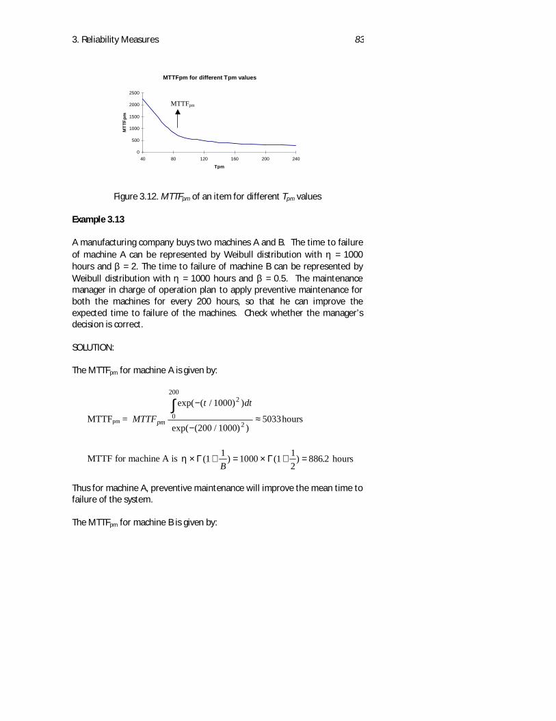
3. Reliability Measures 83
Figure 3.12. MTTFpm of an item for different Tpm values
Example 3.13
A manufacturing company buys two machines A and B. The time to failureof machine A can be represented by Weibull distribution with η = 1000hours and β = 2. The time to failure of machine B can be represented byWeibull distribution with η = 1000 hours and β = 0.5. The maintenancemanager in charge of operation plan to apply preventive maintenance forboth the machines for every 200 hours, so that he can improve theexpected time to failure of the machines. Check whether the manager’sdecision is correct.
SOLUTION:
The MTTFpm for machine A is given by:
MTTFpm = MTTF
t dt
pm
exp( ( / ) )
exp( ( / ) )
−
−≈
∫ 1000
200 10005033
2
0
200
2hours
MTTF for machine A is η × + = × + =Γ Γ( ) ( ) .1 1 1000 1 12
886 2B
hours
Thus for machine A, preventive maintenance will improve the mean time tofailure of the system.
The MTTFpm for machine B is given by:
MTTFpm for different Tpm values
0
500
1000
1500
2000
2500
40 80 120 160 200 240
Tpm
MTT
Fpm
MTTFpm
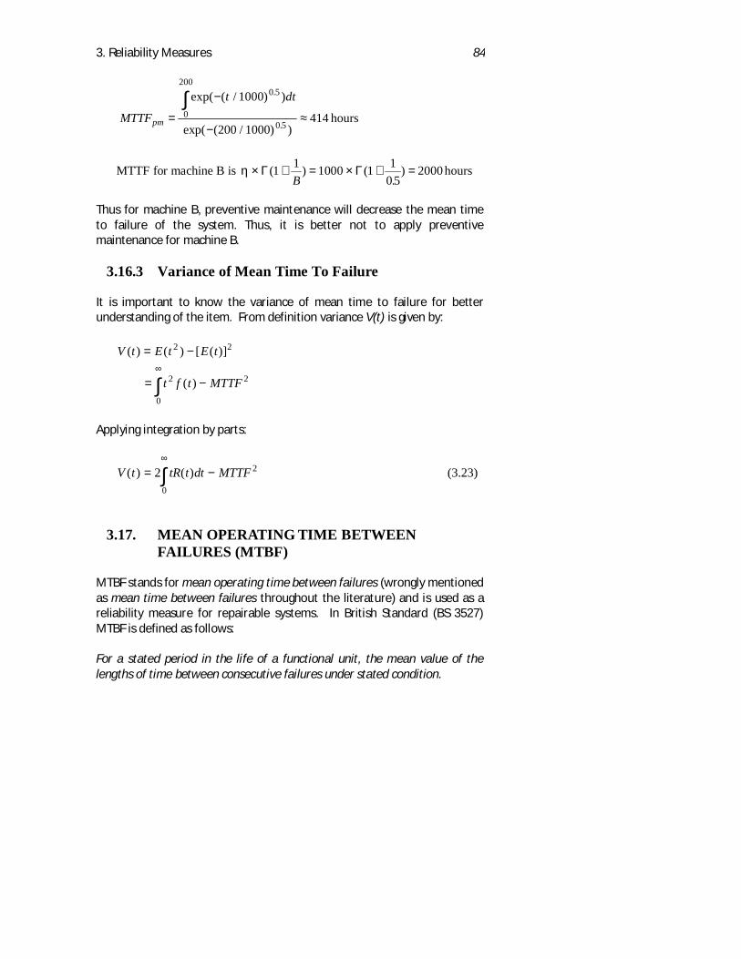
3. Reliability Measures 84
MTTF
t dt
pm =
−
−≈
∫ exp( ( / ) )
exp( ( / ) )
.
.
1000
200 1000414
0 5
0
200
0 5hours
MTTF for machine B is η × + = × + =Γ Γ( ) (.
)1 1 1000 1 10 5
2000B
hours
Thus for machine B, preventive maintenance will decrease the mean timeto failure of the system. Thus, it is better not to apply preventivemaintenance for machine B.
3.16.3 Variance of Mean Time To Failure
It is important to know the variance of mean time to failure for betterunderstanding of the item. From definition variance V(t) is given by:
V t E t E t
t f t MTTF
( ) ( ) [ ( )]
( )
= −
= −∞
∫
2 2
2
0
2
Applying integration by parts:
V t tR t dt MTTF( ) ( )= −∞
∫20
2 (3.23)
3.17. MEAN OPERATING TIME BETWEENFAILURES (MTBF)
MTBF stands for mean operating time between failures (wrongly mentionedas mean time between failures throughout the literature) and is used as areliability measure for repairable systems. In British Standard (BS 3527)MTBF is defined as follows:
For a stated period in the life of a functional unit, the mean value of thelengths of time between consecutive failures under stated condition.
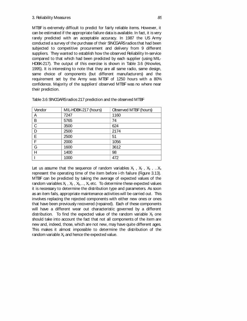
3. Reliability Measures 85
MTBF is extremely difficult to predict for fairly reliable items. However, itcan be estimated if the appropriate failure data is available. In fact, it is veryrarely predicted with an acceptable accuracy. In 1987 the US Armyconducted a survey of the purchase of their SINCGARS radios that had beensubjected to competitive procurement and delivery from 9 differentsuppliers. They wanted to establish how the observed Reliability In-servicecompared to that which had been predicted by each supplier (using MIL-HDBK-217). The output of this exercise is shown in Table 3.6 (Knowles,1995). It is interesting to note that they are all same radio, same design,same choice of components (but different manufacturers) and therequirement set by the Army was MTBF of 1250 hours with a 80%confidence. Majority of the suppliers' observed MTBF was no where neartheir prediction.
Table 3.6 SINCGARS radios 217 prediction and the observed MTBF
Vendor MIL-HDBK-217 (hours) Observed MTBF (hours)A 7247 1160B 5765 74C 3500 624D 2500 2174E 2500 51F 2000 1056G 1600 3612H 1400 98I 1000 472
Let us assume that the sequence of random variables X1 , X2 , X3 , …Xn
represent the operating time of the item before i-th failure (Figure 3.13).MTBF can be predicted by taking the average of expected values of therandom variables X1 , X2 , X3,…, Xn etc. To determine these expected valuesit is necessary to determine the distribution type and parameters. As soonas an item fails, appropriate maintenance activities will be carried out. Thisinvolves replacing the rejected components with either new ones or onesthat have been previously recovered (repaired). Each of these componentswill have a different wear out characteristic governed by a differentdistribution. To find the expected value of the random variable X2 oneshould take into account the fact that not all components of the item arenew and, indeed, those, which are not new, may have quite different ages.This makes it almost impossible to determine the distribution of therandom variable X2 and hence the expected value.
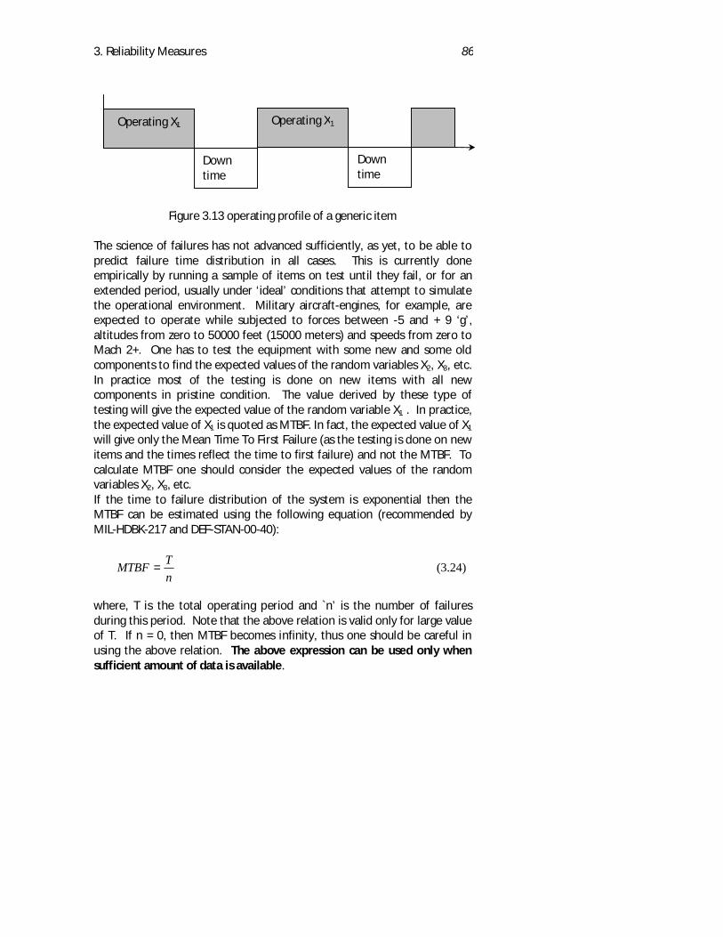
3. Reliability Measures 86
Figure 3.13 operating profile of a generic item
The science of failures has not advanced sufficiently, as yet, to be able topredict failure time distribution in all cases. This is currently doneempirically by running a sample of items on test until they fail, or for anextended period, usually under ‘ideal’ conditions that attempt to simulatethe operational environment. Military aircraft-engines, for example, areexpected to operate while subjected to forces between -5 and + 9 ‘g’,altitudes from zero to 50000 feet (15000 meters) and speeds from zero toMach 2+. One has to test the equipment with some new and some oldcomponents to find the expected values of the random variables X2, X3, etc.In practice most of the testing is done on new items with all newcomponents in pristine condition. The value derived by these type oftesting will give the expected value of the random variable X1 . In practice,the expected value of X1 is quoted as MTBF. In fact, the expected value of X1
will give only the Mean Time To First Failure (as the testing is done on newitems and the times reflect the time to first failure) and not the MTBF. Tocalculate MTBF one should consider the expected values of the randomvariables X2, X3, etc.If the time to failure distribution of the system is exponential then theMTBF can be estimated using the following equation (recommended byMIL-HDBK-217 and DEF-STAN-00-40):
MTBF Tn
= (3.24)
where, T is the total operating period and `n’ is the number of failuresduring this period. Note that the above relation is valid only for large valueof T. If n = 0, then MTBF becomes infinity, thus one should be careful inusing the above relation. The above expression can be used only whensufficient amount of data is available.
Operating X1
Downtime
Downtime
Operating X1
3. Reliability Measures 87
Characteristics of MTBF
1. The value of MTBF is equal to MTTF if after each repair the system is asgood as new.
2. MTBF = 1 / λ for exponential distribution, where λ is the scale parameter( also the hazard function ).
Applications of MTBF
1. For a repairable system, MTBF is the average time in service betweenfailures. Note that, this does not include the time spent at repair facilityby the system.
2. MTBF is used to predict steady-state availability measures like inherentand operational availability.
3.18. PERCENTILE LIFE ( TTFP OR BP% )
Percentile life or Bp% is a measure of reliability which is popular amongindustries. This is the life by which certain proportion of the population (p%) can be expected to have failed. B10% means the life (time) by which 10%of the items will be expected to have failed. Percentile life is nowfrequently used among aerospace industries as a design requirement.Mathematically percentile life can be obtained by solving the followingequation for t:
F t f x dx pt
( ) ( ) %= =∫0
(3.25)
Assume that F(t) is a exponential distribution with parameter λ = 0.05, andwe are interested in finding B10 . Then from above equation we have:
1 0 05 010 2107− − = ⇒ =exp( . ) . .t t
Thus 2.107 is the B10 life for exponential distribution with parameter 0.05.The main application of percentile life lies in prediction of initial sparesrequirement (initial spares provisioning, IP).
3. Reliability Measures 88
System Reliabilityand MaintainabilityCourse material
Course Instructor: Professor U Dinesh KumarIndian Institute of Management Bangalore
4. Systems Reliability 89
Chapter 4
Systems Reliability
'A Bird is an instrument working according to a mathematical law. It lies withinthe power of man to make this instrument with all its motion'
Leonardo da Vinci
In this chapter, we present methodologies that can be used to evaluatesystems reliability using simple mathematical tools. The chapter discussestwo approaches that can be used to predict the reliability metrics of thesystem. First, we study the models that are based on simple probabilitytheory, assuming that the time-to-failure distributions of differentcomponents within the system are known. These models can be used onlyfor non-repairable items. The second approach is based on Markov models,for predicting different reliability measures. The models for repairableitems will be discussed using the Markov models. Throughout the Chapter,the word ‘system’ is used to represent the complete equipment and theword ‘item’ is used as a generic term that stands for subsystem, module,component, part or unit. Any reliability prediction methodology using time-to-failure approach will involve the following steps:1. Construct the reliability block diagram (RBD) of the system. This may
involve performing failure modes and effect analysis (FMEA).2. Determine the operational profile of each block in the reliability block
diagram.3. Derive the time-to-failure distribution of each block.4. Derive the life exchange rate matrix (LERM) for the different
components within the system.5. Compute reliability function of each block.
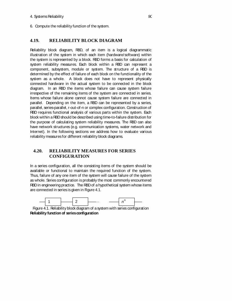
4. Systems Reliability 90
6. Compute the reliability function of the system.
4.19. RELIABILITY BLOCK DIAGRAM
Reliability block diagram, RBD, of an item is a logical diagrammaticillustration of the system in which each item (hardware/software) withinthe system is represented by a block. RBD forms a basis for calculation ofsystem reliability measures. Each block within a RBD can represent acomponent, subsystem, module or system. The structure of a RBD isdetermined by the effect of failure of each block on the functionality of thesystem as a whole. A block does not have to represent physicallyconnected hardware in the actual system to be connected in the blockdiagram. In an RBD the items whose failure can cause system failureirrespective of the remaining items of the system are connected in series.Items whose failure alone cannot cause system failure are connected inparallel. Depending on the item, a RBD can be represented by a series,parallel, series-parallel, r-out-of-n or complex configuration. Construction ofRBD requires functional analysis of various parts within the system. Eachblock within a RBD should be described using time-to-failure distribution forthe purpose of calculating system reliability measures. The RBD can alsohave network structures (e.g. communication systems, water network andInternet). In the following sections we address how to evaluate variousreliability measures for different reliability block diagrams.
4.20. RELIABILITY MEASURES FOR SERIESCONFIGURATION
In a series configuration, all the consisting items of the system should beavailable or functional to maintain the required function of the system.Thus, failure of any one item of the system will cause failure of the systemas whole. Series configuration is probably the most commonly encounteredRBD in engineering practice. The RBD of a hypothetical system whose itemsare connected in series is given in Figure 4.1.
Figure 4.1. Reliability block diagram of a system with series configurationReliability function of series configuration
1 2 n n…
4. Systems Reliability 91
Reliability function of a system with series configuration can be derivedfrom the reliability function of its consisting items. Let RS(t) represent thereliability function of a series system with n items. Let Ri(t) denote thereliability function of the item i. If TTFi is the time-to-failure randomvariable for the item i, then the reliability function of system for ‘t’ hours ofoperation is given by:
RS (t) = P [ TTF1 ≥ t, TTF2 ≥ t, ...., TTFn ≥ t ] (4.1)
The equation (4.1) clearly states that the system under consideration willmaintain the required function if and only if all the n items of the systemare able to maintain the required function for at least t hours of operation.Assuming that the random variables TTFi are independent of each other,the expression (4.1) can be written as:
Rs(t) = P[TTF1 ≥ t ] × P[TTF2 ≥ t ] × ... × P[ TTFn ≥ t ] = R1(t) × R2(t) × ... × Rn(t)
Thus, the reliability of a series configuration with n items is given by:
R t R ts ii
n( ) ( )= ∏
=1(4.2)
Note that in the above equation (4.2), it is assumed that the connectingmedia (such as solder joints) between different items is 100% reliable(unless this is specifically included in the RBD). However, this need not betrue. In the equation (4.2) time t is used as a generic term. In most casetime actually represents age or utilisation of the item under consideration.It can have different units such as hours, miles, landings, cycles etc fordifferent items. One has to normalise the ‘time’ before calculating thereliability function in such cases. One method of normalising the differentlife units of the items is using Life Exchange Rate Matrix (LERM), which willbe discussed later in this chapter. When the life units of items are different(or different items have different utilisation), we use the following equationto find the reliability of the series system.
R P TTF t TTF t TTF t R t R t R ts n n n n= ≥ ≥ ≥ = × × ×[ , , , ] ( ) ( ) ( )1 1 2 2 1 1 2 2L L
That is,
4. Systems Reliability 92
∏=
=n
iiiS tRtR
1
)()( (4.3)
In equation (4.3), ti is the age of the item i, which is equivalent to age t ofthe system. That is, for the system to survive up to age t, the item i shouldsurvive up to ti. Throughout this book we use equation (4.3) unlessotherwise specified.Characteristics of reliability function of a series configuration1. The value of the reliability function of the system, RS(t), for a seriesconfiguration is less than or equal to the minimum value of the individualreliability function of the constituting items. That is:
R t Min R tSi n
i( ) { ( )},2,..
≤=1
2. If hi(t) represent the hazard function of item i, then the system reliabilityof a series system can be written as:
dxxh
dxxhtR
t n
ii
n
i
tis
])([exp(
)(exp()(
0 1
1 0
∫ ∑−=
∏ ∫−=
=
=
Example 4.1A system consists of four items, each of them are necessary to maintain therequired function of the system. The time to failure distribution and theircorresponding parameter values are given in Table 4.1. Find the reliabilityof the system for 500 and 750 hours of operation.
Table 4.1 Time to failure distribution and their parameter of the itemsItem Time to failure distribution Parameter values
Item 1 Exponential λ = 0.001
Item 2 Weibull η = 1200 hours β = 3.2
Item 3 Normal µ = 800 hours σ = 350
Item 4 Weibull η = 2000 hours β = 1.75
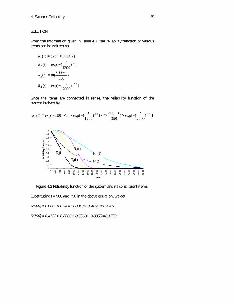
4. Systems Reliability 93
SOLUTION:
From the information given in Table 4.1, the reliability function of variousitems can be written as:
R t t
R t t
R t t
R t t
1
23 2
3
41 75
0 001
1200800
350
2000
( ) exp( . )
( ) exp[ ( ) ]
( ) ( )
( ) exp[ ( ) ]
.
.
= − ×
= −
=−
= −
Φ
Since the items are connected in series, the reliability function of thesystem is given by:
R t t t t ts ( ) exp( . ) exp[ ( ) ] ( ) exp[ ( ) ]. .= − × × − × − × −0 001
1200800
350 20003 2 1 75Φ
Figure 4.2 Reliability function of the system and its constituent items.
Substituting t = 500 and 750 in the above equation, we get:
R(500) = 0.6065 × 0.9410 × 8043 × 0.9154 = 0.4202
R(750) = 0.4723 × 0.8003 × 0.5568 × 0.8355 = 0.1759
00.1
0.20.30.4
0.50.60.7
0.80.9
1
0
200
400
600
800
1000
1200
1400
1600
1800
2000
2200
2400
2600
2800
3000
3200
3400
3600
3800
4000
Time
Relia
bilit
y fu
nctio
n
R4 (t)R3(t)
R1(t)R2(t)
Rs(t)
4. Systems Reliability 94
Figure 4.2 shows the reliability function of the system and various items ofthe system. Note that the system reliability value is always less than orequal to any of the constituting items.
Example 4.2
Avionics system of an aircraft consists of digital auto-pilot, integrated globalpositioning system, weather and ground mapping radar, digital map displayand warning system. Apart from the above items, the avionics system hascontrol software. The time-to-failure distributions of various items are givenin Table 4.2. Find the reliability of the avionics system for 100 hours ofoperation if all the items are necessary to maintain the required function ofthe avionics system.
Table 4.2 Time-to-failure distribution of various items of the avionics system
Item Time-to-failuredistribution
Parameter values
Digital autopilot Exponential λ = 0.003
Integrated globalpositioning system
Weibull η = 1200, β = 3.2
Weather and groundmapping radar
Weibull η = 1000, β = 2.1
Digital map display Normal µ = 800, σ = 120
Warning System Normal µ = 1500, σ = 200
Software Exponential λ = 0.001
SOLUTION:
From the data given in Table 4.2, we can derive the reliability function ofvarious items as follows:
1. Reliability of digital auto-pilot
R t t R1 1 100 0 003 100 0 7408( ) exp( ) ( ) exp( . ) .= − × ⇒ = − × =λ
4. Systems Reliability 95
2. Reliability of integrated global positioning system.
R t R2 23 2100 100 100 1200 0 9996( ) exp( ( / ) ) ( ) exp( ( / ) ) ..= − ⇒ = − =η β
3. Reliability of weather and ground mapping system radar
R t R3 32 1100 100 100 1000 0 9920( ) exp( ( / ) ) ( ) exp( ( / ) ) ..= − ⇒ = − =η β
4. Reliability of digital map display
R t R4 4100 100 800 100120
58 1( ) ( ) ( ) ( ) ( . )=−
⇒ =−
= =Φ Φ Φµ
σ
5. Reliability of warning system
R t R5 4100 100 1500 100200
7 1( ) ( ) ( ) ( ) ( )=−
⇒ =−
= =Φ Φ Φµ
σ
6. Reliability of software
R t t6 0 001 100 0 9048( ) exp( ) exp( . ) .= − ⇒ − × =λ
Thus, the reliability of the avionics system for 100 hours of operation isgiven by:
R Rs ii
( ) ( ) . . . . .100 100 0 7408 0 9996 0 9920 1 1 0 9048 0 66461
6= = × × × × × =
=∏
Hazard function of a series configuration
Let RS(t) denote the reliability function of the system. From definition, thehazard rate of the system, hS(t), can be written as:
h t dR tdt R tSS
S( )
( )( )
= − ×1
(4.4)
Using equation (4.2), the expression for RS(t) can be written as:
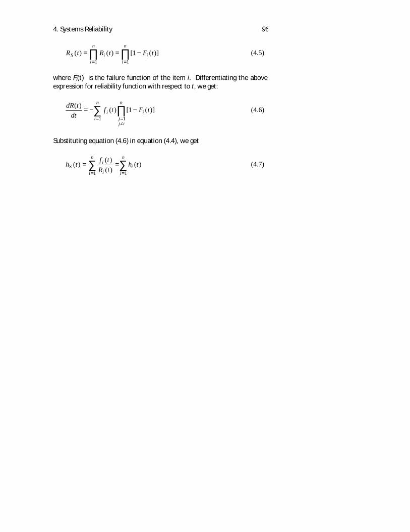
4. Systems Reliability 96
R t R t F tS ii
n
ii
n( ) ( ) [ ( )]= = −
= =∏ ∏
1 11 (4.5)
where Fi(t) is the failure function of the item i. Differentiating the aboveexpression for reliability function with respect to t, we get:
dR tdt
f t F tii
n
ijj i
n( ) ( ) [ ( )]= − −= =
≠
∑ ∏1 1
1 (4.6)
Substituting equation (4.6) in equation (4.4), we get
h t f tR t
h tSi
ii
n
ii
n( ) ( )
( )( )= =
= =∑ ∑
1 1
(4.7)
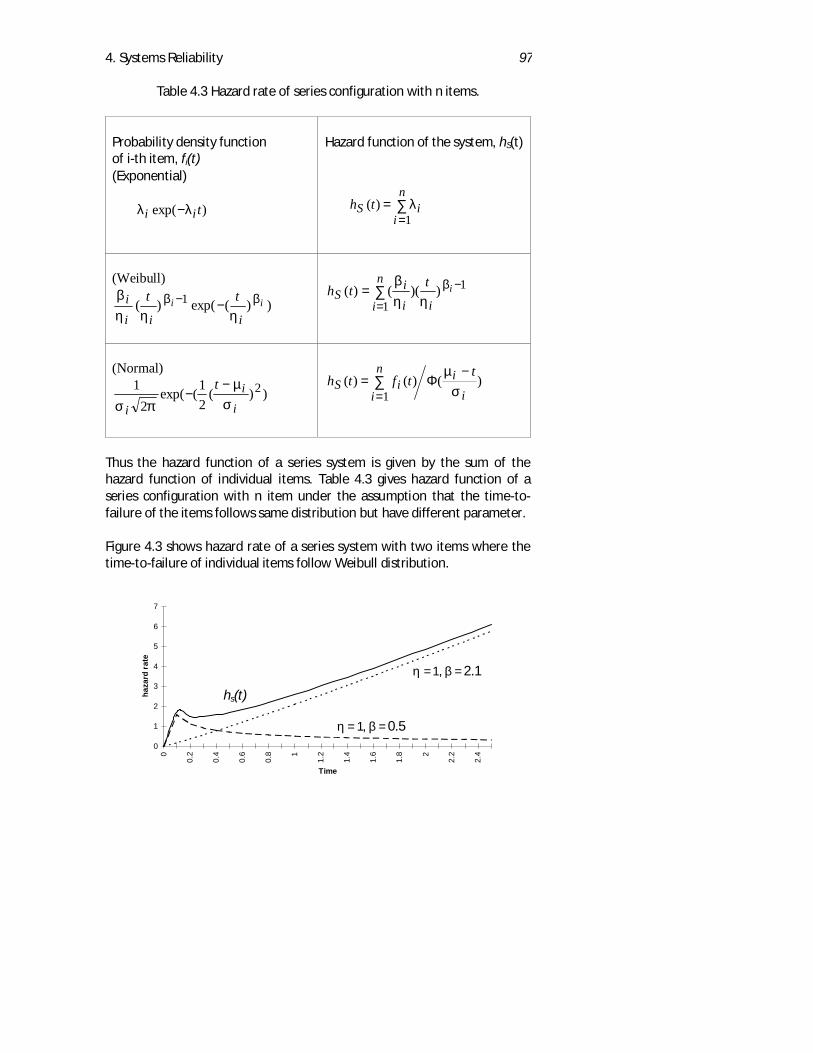
4. Systems Reliability 97
Table 4.3 Hazard rate of series configuration with n items.
Probability density functionof i-th item, fi(t)
Hazard function of the system, hS(t)
(Exponential)
)exp( tii λλ − ∑=
=n
iiS th
1)( λ
(Weibull)
))(exp()( 1 ii
iiii tt ββ
ηηηβ
−− ∑=
−=n
i iii
S itth1
1))(()( βηη
β
(Normal)
))(21(exp(
21 2
ii
i
tσ
µ
πσ
−−
∑=
−Φ=
n
i ii
iSt
tfth1
)()()(σ
µ
Thus the hazard function of a series system is given by the sum of thehazard function of individual items. Table 4.3 gives hazard function of aseries configuration with n item under the assumption that the time-to-failure of the items follows same distribution but have different parameter.
Figure 4.3 shows hazard rate of a series system with two items where thetime-to-failure of individual items follow Weibull distribution.
0
1
2
3
4
5
6
7
0
0.2
0.4
0.6
0.8 1
1.2
1.4
1.6
1.8 2
2.2
2.4
Time
haza
rd ra
te
hs(t)
η = 1, β = 2.1
η = 1, β = 0.5
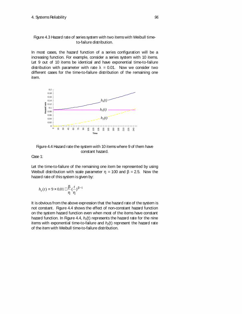
4. Systems Reliability 98
Figure 4.3 Hazard rate of series system with two items with Weibull time-to-failure distribution.
In most cases, the hazard function of a series configuration will be aincreasing function. For example, consider a series system with 10 items.Let 9 out of 10 items be identical and have exponential time-to-failuredistribution with parameter with rate λ = 0.01. Now we consider twodifferent cases for the time-to-failure distribution of the remaining oneitem.
Figure 4.4 Hazard rate the system with 10 items where 9 of them haveconstant hazard.
Case 1:
Let the time-to-failure of the remaining one item be represented by usingWeibull distribution with scale parameter η = 100 and β = 2.5. Now thehazard rate of this system is given by:
h t ts ( ) . ( )= × + −9 0 01 1β
η ηβ
It is obvious from the above expression that the hazard rate of the system isnot constant. Figure 4.4 shows the effect of non-constant hazard functionon the system hazard function even when most of the items have constanthazard function. In Figure 4.4, h1(t) represents the hazard rate for the nineitems with exponential time-to-failure and h2(t) represent the hazard rateof the item with Weibull time-to-failure distribution.
0
0.02
0.04
0.06
0.08
0.1
0.12
0.14
0.16
0.18
0.2
0 15 30 45 60 75 90 105
120
135
150
165
180
195
210
225
240
Time
Haz
ard
rate
h1(t)
h2(t)
hs(t)
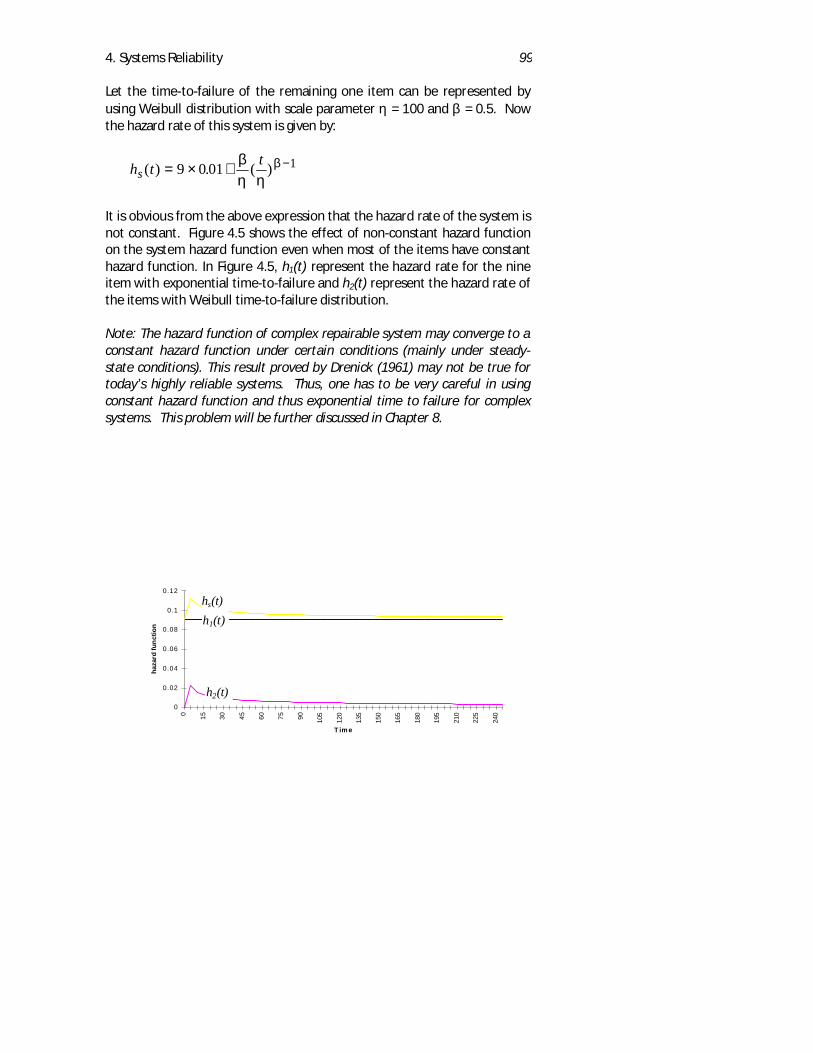
4. Systems Reliability 99
Let the time-to-failure of the remaining one item can be represented byusing Weibull distribution with scale parameter η = 100 and β = 0.5. Nowthe hazard rate of this system is given by:
h t ts ( ) . ( )= × + −9 0 01 1β
η ηβ
It is obvious from the above expression that the hazard rate of the system isnot constant. Figure 4.5 shows the effect of non-constant hazard functionon the system hazard function even when most of the items have constanthazard function. In Figure 4.5, h1(t) represent the hazard rate for the nineitem with exponential time-to-failure and h2(t) represent the hazard rate ofthe items with Weibull time-to-failure distribution.
Note: The hazard function of complex repairable system may converge to aconstant hazard function under certain conditions (mainly under steady-state conditions). This result proved by Drenick (1961) may not be true fortoday’s highly reliable systems. Thus, one has to be very careful in usingconstant hazard function and thus exponential time to failure for complexsystems. This problem will be further discussed in Chapter 8.
0
0.02
0.04
0.06
0.08
0.1
0.12
0 15 30 45 60 75 90 105
120
135
150
165
180
195
210
225
240
T im e
haza
rd fu
nctio
n
hs(t)h1(t)
h2(t)
4. Systems Reliability 100
Figure 4.5 Hazard function of the system with 10 items where 9 of themhave constant hazard.
Example 4.3
A system has two items A and B connected in series. The time-to-failure ofitem A follows exponential distribution with parameter λ = 0.002. The time-to-failure of item B follows Weibull distribution with parameter η = 760 andβ = 1.7. Find the hazard rate of this system at time t = 100 and t = 500.
SOLUTION:
Let hA(t) and hB(t) represent the hazard rate of item A and B respectively.Since the items are connected in series, the hazard rate of the system, hS(t)is given by:
7.01 )760
)(760
7.1(002.0))(()()()( ttththth BAS +=+=+= −β
ηηβ
λ
Substituting t = 100 and t = 500 in the above equation,
hS(100) = 0.00254
hS(500) = 0.0036
Mean time to failure of a series configuration
The mean time to failure, MTTF, of a series configuration, denoted byMTTFS, can be written as:
∫ ∏=∫=∞
=
∞
0 10)( dttRdtRMTTF
n
iiSS (4.8)
The above integral can be evaluated using numerical integration if thefailure distribution is Weibull, normal, lognormal or Gamma. However, incase of exponential distribution the expression for system MTTFS can beobtained as follows. Assume that the time-to-failure distribution ofcomponent i is given by,1− −exp( ).λ i t Substituting R t ti i( ) exp( )= −λ inequation (4.8) we have,
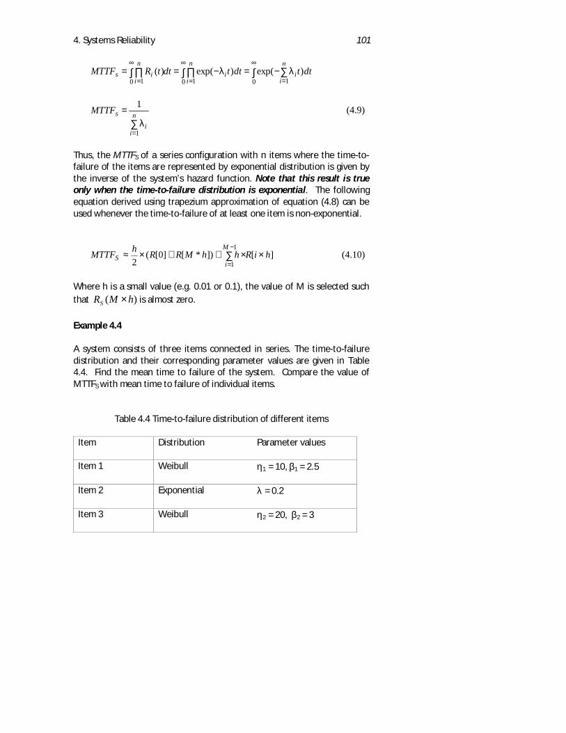
4. Systems Reliability 101
∫ ∫ ∑∏∫ ∏∞ ∞
==
∞
=−=−==
0 0 110 1)exp()exp()( dttdttdttRMTTF
n
ii
n
ii
n
iis λλ
∑=
= n
ii
sMTTF
1
1
λ(4.9)
Thus, the MTTFS of a series configuration with n items where the time-to-failure of the items are represented by exponential distribution is given bythe inverse of the system’s hazard function. Note that this result is trueonly when the time-to-failure distribution is exponential. The followingequation derived using trapezium approximation of equation (4.8) can beused whenever the time-to-failure of at least one item is non-exponential.
][])*[]0[(2
1
1hiRhhMRRhMTTF
M
iS ××++×≈ ∑
−
=(4.10)
Where h is a small value (e.g. 0.01 or 0.1), the value of M is selected suchthat )( hMRS × is almost zero.
Example 4.4
A system consists of three items connected in series. The time-to-failuredistribution and their corresponding parameter values are given in Table4.4. Find the mean time to failure of the system. Compare the value ofMTTFS with mean time to failure of individual items.
Table 4.4 Time-to-failure distribution of different items
Item Distribution Parameter values
Item 1 Weibull η1 = 10, β1 = 2.5
Item 2 Exponential λ = 0.2
Item 3 Weibull η2 = 20, β2 = 3
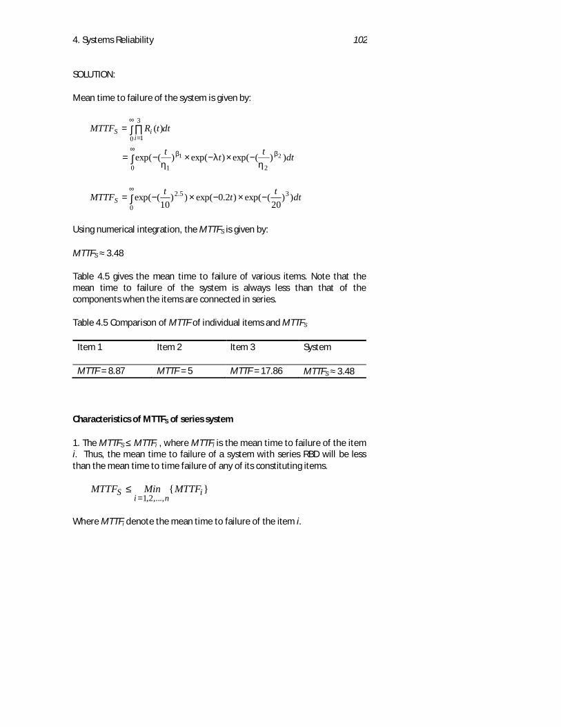
4. Systems Reliability 102
SOLUTION:
Mean time to failure of the system is given by:
dtttt
dttRMTTFi
iS
))(exp()exp()(exp(
)(
21
210
0
3
1
ββ
ηλ
η−×−×−=
=
∫
∫ ∏
∞
∞
=
∫∞
−×−×−=0
35.2 ))20
(exp()2.0exp())10
(exp( dttttMTTFS
Using numerical integration, the MTTFS is given by:
MTTFS ≈ 3.48
Table 4.5 gives the mean time to failure of various items. Note that themean time to failure of the system is always less than that of thecomponents when the items are connected in series.
Table 4.5 Comparison of MTTF of individual items and MTTFS
Item 1 Item 2 Item 3 System
MTTF = 8.87 MTTF = 5 MTTF = 17.86 MTTFS ≈ 3.48
Characteristics of MTTFS of series system
1. The MTTFS ≤ MTTFi , where MTTFi is the mean time to failure of the itemi. Thus, the mean time to failure of a system with series RBD will be lessthan the mean time to time failure of any of its constituting items.
MTTF Min MTTFSi n
i≤=1,2,...,
{ }
Where MTTFi denote the mean time to failure of the item i.
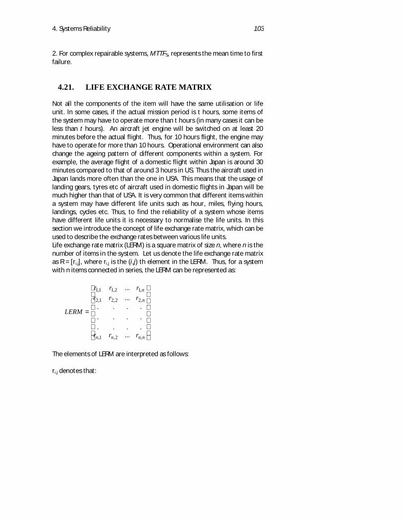
4. Systems Reliability 103
2. For complex repairable systems, MTTFS, represents the mean time to firstfailure.
4.21. LIFE EXCHANGE RATE MATRIX
Not all the components of the item will have the same utilisation or lifeunit. In some cases, if the actual mission period is t hours, some items ofthe system may have to operate more than t hours (in many cases it can beless than t hours). An aircraft jet engine will be switched on at least 20minutes before the actual flight. Thus, for 10 hours flight, the engine mayhave to operate for more than 10 hours. Operational environment can alsochange the ageing pattern of different components within a system. Forexample, the average flight of a domestic flight within Japan is around 30minutes compared to that of around 3 hours in US. Thus the aircraft used inJapan lands more often than the one in USA. This means that the usage oflanding gears, tyres etc of aircraft used in domestic flights in Japan will bemuch higher than that of USA. It is very common that different items withina system may have different life units such as hour, miles, flying hours,landings, cycles etc. Thus, to find the reliability of a system whose itemshave different life units it is necessary to normalise the life units. In thissection we introduce the concept of life exchange rate matrix, which can beused to describe the exchange rates between various life units.Life exchange rate matrix (LERM) is a square matrix of size n, where n is thenumber of items in the system. Let us denote the life exchange rate matrixas R = [ri,j], where ri,j is the (i,j) th element in the LERM. Thus, for a systemwith n items connected in series, the LERM can be represented as:
=
nnnn
n
n
rrr
rrrrrr
LERM
,2,1,
,22,21,2
,12,11,1
......
.
.
.
.
.
.
.
.
.......
The elements of LERM are interpreted as follows:
ri,j denotes that:
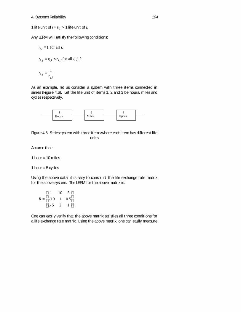
4. Systems Reliability 104
1 life unit of i = ri,j × 1 life unit of j.
Any LERM will satisfy the following conditions:
1, =iir for all i.
jkkiji rrr ,,, ×= for all i, j, k
ijji r
r,
,1
=
As an example, let us consider a system with three items connected inseries (Figure 4.6). Let the life unit of items 1, 2 and 3 be hours, miles andcycles respectively.
Figure 4.6. Series system with three items where each item has different lifeunits
Assume that:
1 hour = 10 miles
1 hour = 5 cycles
Using the above data, it is easy to construct the life exchange rate matrixfor the above system. The LERM for the above matrix is:
=
125/15.0110/1
5101R
One can easily verify that the above matrix satisfies all three conditions fora life exchange rate matrix. Using the above matrix, one can easily measure
1Hours
2Miles
3Cycles
4. Systems Reliability 105
reliability characteristics in normalised life unit. For the RBD shown inFigure 4.6, reliability of the system for 5 cycles is given by R1(1)×R2(1)×R3(5).
Example 4.5
Reliability block diagram of a system consists of three modules A, B and Cconnected in series. The time-to-failure of module A follows Weibulldistribution with scale parameter η = 100 hours and β = 3.2. The time-to-failure of module B follows Normal distribution with parameter µ = 400cycles and σ = 32 cycles. The time-to-failure of module C followsexponential distribution with parameter λ = 0.00015 per mile. It was alsonoted that, during 1 hour, the module B performs 12 cycles and module Cperforms 72 miles. Find the probability that the system will survive up to240 cycles of module B.
SOLUTION:
For the system to survive 240 cycles, module A should survive up to 20hours and module C should survive up to 1440 miles.
The reliability of individual modules are given by:
9942.0))10020(exp())(exp()( 2.3 =−=−= β
ηA
AAttR
1)32
240400()()( =−
Φ=−
Φ=σ
µ BBB
ttR
8174.0)144000015.0exp()exp()( =×−=×−= CCC ttR λ
The system reliability for 240 cycles is given by:
8126.08174.019942.0)1440()240()20()240( =××=××= CBAS RRRR
4.22. PARALLEL CONFIGURATION
In a parallel configuration the system fails only when all the items of thesystem fail. In other words, to maintain the required function only one item
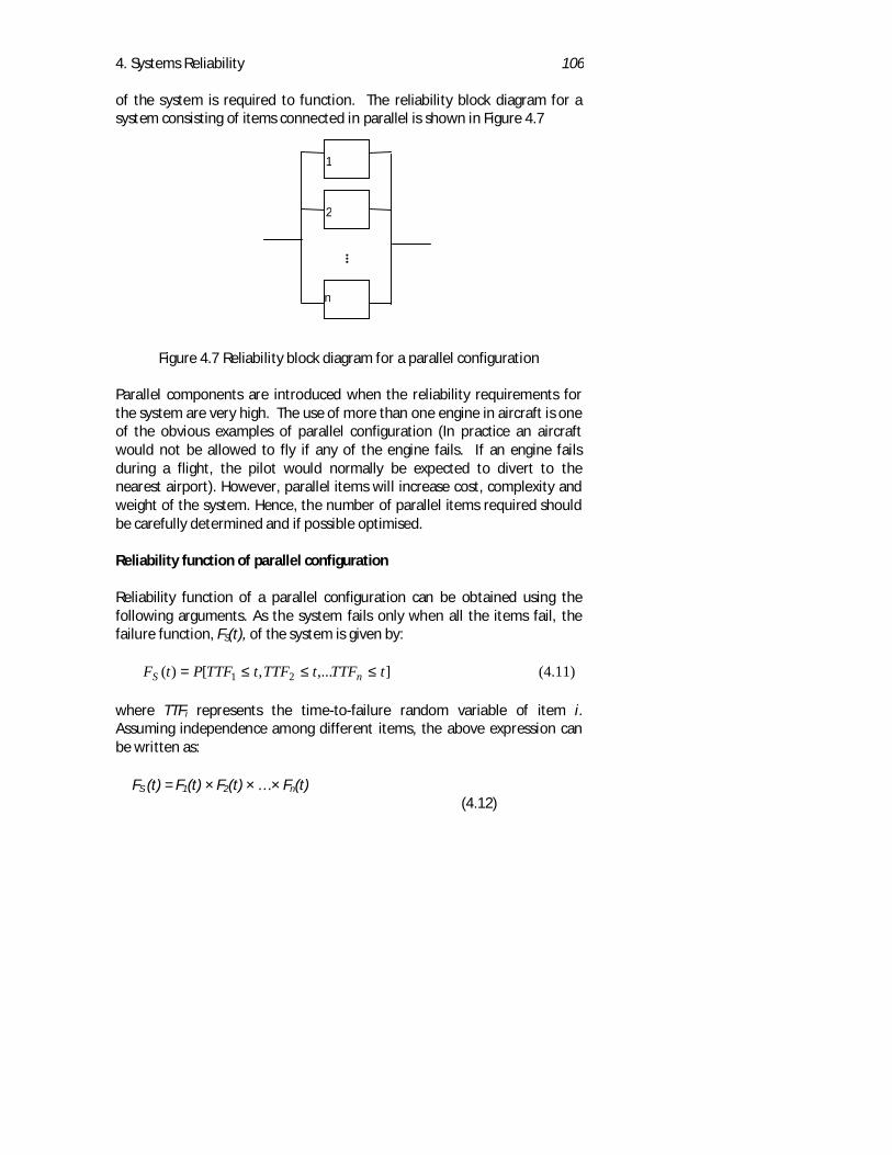
4. Systems Reliability 106
of the system is required to function. The reliability block diagram for asystem consisting of items connected in parallel is shown in Figure 4.7
Figure 4.7 Reliability block diagram for a parallel configuration
Parallel components are introduced when the reliability requirements forthe system are very high. The use of more than one engine in aircraft is oneof the obvious examples of parallel configuration (In practice an aircraftwould not be allowed to fly if any of the engine fails. If an engine failsduring a flight, the pilot would normally be expected to divert to thenearest airport). However, parallel items will increase cost, complexity andweight of the system. Hence, the number of parallel items required shouldbe carefully determined and if possible optimised.
Reliability function of parallel configuration
Reliability function of a parallel configuration can be obtained using thefollowing arguments. As the system fails only when all the items fail, thefailure function, FS(t), of the system is given by:
],...,[)( 21 tTTFtTTFtTTFPtF nS ≤≤≤= (4.11)
where TTFi represents the time-to-failure random variable of item i.Assuming independence among different items, the above expression canbe written as:
FS (t) = F1(t) × F2(t) × … × Fn(t) (4.12)
1
2
n
4. Systems Reliability 107
where Fi(t) is the time to failure distribution of item i. Substituting Fi(t)=1 -Ri(t) in equation (4.12), the expression for failure function of a parallelconfiguration can be written as:
FS (t) = [ 1 - R1(t) ] × [ 1 - R2(t) ] × … × [1 - Rn(t) ] (4.13)
Now, the reliability function, RS(t), of a parallel configuration can be writtenas:
RS(t) = 1 - FS (t) = 1 - [1 - R1(t)] × [1 - R2(t)] × … × [1 -Rn(t)]
or
∏=
−−=n
iiS tRtR
1)](1[1)( (4.14)
Characteristics of a parallel configuration
1. The system reliability, RS(t), is more than reliability of the any of theconsisting items. That is,
RS(t) ≥ )}({,...,1
tRMax ini=
2. If hi(t) represent the hazard rate of item i, then the reliability function ofa parallel configuration can be written as:
∏ ∫=
−−−=n
i
t
iS dtthtR1 0
])(exp(1[1)(
Example 4.6A fly-by-wire aircraft has four flight control system electronics (FCSE)connected in parallel. The time-to-failure of FCSE can be represented byWeibull distribution with scale parameter η=2800 and β = 2.8. Find thereliability of flight control system for 1000 hours of operation.
SOLUTION:
Reliability function for a parallel system with four identical items is given by:
4. Systems Reliability 108
R t R t
R t
S ii
( ) [ ( )]
[ ( )]
= − −∏
= − −
=1 1
1 11
4
4
where R(t) is the reliability function of each item. For t = 1000, R(t) is givenby:
9455.0))2800/1000(exp())/(exp()( 8.2 =−=−= βηttR
Thus the reliability of flight control system for 1000 hours of operation isgiven by:
999991.0]9455.01[1)1000( 4 =−−=SR
Hazard function of a parallel configuration
Hazard function, hS(t), of the parallel configuration can be written as:
)(1)(
)(tRdt
tdRth
S
SS ×
−= (4.15)
Substituting the expression for RS(t) from equation (4.14) in the aboveequation, we get
∏∏
=
= −−×−−−=
n
ii
n
iiS
tRtR
dtdth
1
1 ))](1(1[
1}))](1(1[{)( (4.16)
It is easy to verify that the above equation can be written as:
∏
∑ ∏
=
= ≠=
−−
×= n
ii
n
j
n
jiiij
StR
tFtfth
1
1 ,1
)](1[1
})()({)( (4.17)
Where, fi(t) is the probability density function of item i.
Example 4.7
4. Systems Reliability 109
For the flight control system electronics discussed in the example 3.5, findthe hazard function of the system at time t = 100.
SOLUTION:
Since all the four items are identical, the hazard rate of the system can bewritten as (using equation (3.15)):
4
3
)]([1)]([)(4)(
tFtFtfthS
−
××=
where,
))(exp()(
))(exp()()( 1
β
ββ
η
ηηηβ
ttF
tttf
−=
−= −
Substituting t = 100, we get
hS(t) = 8.0 × 10 - 8
Mean time to failure of parallel configuration
The mean time to failure of a parallel configuration, denoted by MTTFS, canbe written as:
∫ ∏∫∞
=
∞−−==
0 10)]}(1[1{ dttRdtRMTTF
n
iiSS (4.18)
For most of the failure distributions one may have to use numericalintegration to evaluate the above integral. However, in case of exponentialdistribution we can get simple expression for system’s MTTF.
Assume that the time-to-failure distribution of component i isexponential with mean )/1( iλ . Then the mean time to failure of the
system, MTTFS, is given by:
4. Systems Reliability 110
∫ ∏∫ ∏∞
=
∞
=−−−==
0 10 1)]}exp(1[1{)(
n
ii
n
iis dttdttRMTTF λ (4.19)
For particular values of n, we can simplify the above integral to derive theexpression for the MTTFS.
Case 1: Assume n = 2. Equation (4.19) can be written as:
2121
02121
20
1
111
)])(exp()exp()[exp(
))]}exp(1())exp(1[(1{
λλλλ
λλλλ
λλ
+−+=
+−−−+−=
−−⋅−−−=
∫
∫
∞
∞
dtttt
dtttMTTFS
Case 2: Assume n = 3, the expression for MTTFS can be written as:
321323121321
0
3
1
1111111
))]}exp(1([[1{
λλλλλλλλλλλλ
λ
+++
+−
+−
+−++=
−−−= ∫ ∏∞
=dttMTTF i
iS
(4.20)
4.23. R-OUT-OF-N SYSTEMS
In an r-out-of-n (or r-out-of-n:G) system, at least r items out of the total nitems should maintain their required function for the system to beoperational. Following are few examples of r-out-of-n systems:1. Control software in a space shuttle has four programs. For the successful
completion of the mission, at least three of them should maintain therequired function and also the output from at least three programs shouldagree with each other. This is an example of a 3-out-of-4 system.
2. Most of the telecommunication system can be represented as a r-out-of-nsystems.
The reliability function of r-out-of-n system can be derived as stated below.
4. Systems Reliability 111
Reliability function of an r-out-of-n system
Consider an r-out-of-n system with identical items. That is, R1(t)=R2(t)=... =Rn(t). Then the system reliability, RS(t,r,n), is given by:
inin
riS tRtR
in
nrtR −
=−
= ∑ )](1[)]([),,( (4.21)
For the cases when the time-to-failure distribution is exponential or Weibullwe have the following expressions for reliability function.
1. Exponential time-to-failure distribution
∑=
−−−−
=
n
ri
iniS tt
in
nrtR ]exp(1[)][exp(),,( λλ
2. Weibull time-to-failure distribution
∑=
−−−−
=
n
ri
iniS
ttin
nrtR )])(exp(1[)])([exp(),,( ββ
ηη
However, if the items are not identical then one may have to use othermathematical models such as enumeration to evaluate the reliability. Forexample consider a 2-out-of-3 system with non-identical items. Thereliability function of the system can be derived as follows.Let Ei denote the event that the item i successfully completes the mission(or survives t hours of operation). Then the reliability function for thesystem can be written as:
RS(t) = P [{E1 ∩ E2} ∪ {E1 ∩ E3 } ∪ {E2 ∩ E3 }]
By putting, A = E1 ∩ E2 , B = E1 ∩ E3 and C = E2 ∩ E3, the above expressioncan be written as:
RS(t,2,3) = P [ {A ∪ B ∪ C } ]
= P(A) + P(B) + P(C) - P(A ∩ B) - P(A ∩ C) - P(B ∩ C)+ P(A ∩ B ∩ C)
4. Systems Reliability 112
= P(E1∩E2 ) + P(E1∩ E3 ) + P(E2 ∩ E3 ) - 2 P( E1∩ E2∩E3 )
Let Ri (t) represent the reliability function for the item i. Now the aboveexpression can be written as:
RS (t, 2, 3) = R1(t) R2(t) + R1(t) R3(t) + R2(t) R3(t) - 2 × R1(t) R2(t) R3(t)
The above approach becomes complex when the number of items nincreases. However, there are several approaches available to tacklecomplex r-out-of-n systems with non-identical items. The reliability functionof r-1-out-of-n and r-out-of-n system with identical items satisfies thefollowing relation:
),,()](1[)]([1
),1,( 11 nrtRtRtRrn
nrtR Srnr
s +−
−
=− +−− (4.22)
Mean Time to Failure of r-out-of-n Systems
The mean time to failure, MTTF, of an r-out-of-n system, MTTFS(r,n), can beobtained using the following expression:
∫∞
=0
),,(),( dtnrtRnrMTTF SS
One may have to use numerical integration in most of the cases to evaluatethe above integral. However, if the time-to-failure distribution isexponential, then the above integral reduces to a simple expression. Forexample, consider a 2-out-of-3 system with identical items where the time-to-failure distribution of the item is represented by exponential distributionwith parameter λ. The reliability function of 2-out-of-3 system withexponential items are given by:
)3exp())exp(1)(2exp(3
)]exp(1[)][exp(3
)(3
2
ttt
tti
tRi
iniS
λλλ
λλ
−+−−−=
−−−
= ∑
=
−
Now the MTTFS is given by,
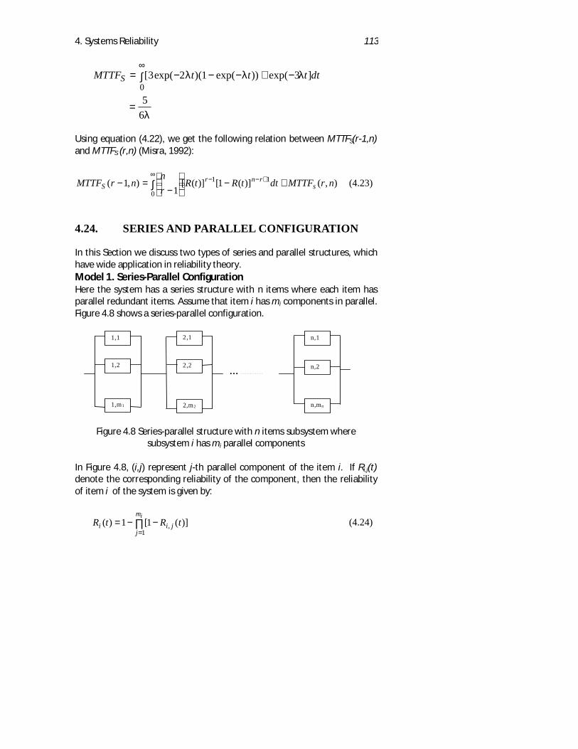
4. Systems Reliability 113
MTTF t t t dtS = − − − + −∫
=
∞[ exp( )( exp( )) exp( ]3 2 1 3
56
0λ λ λ
λ
Using equation (4.22), we get the following relation between MTTFS(r-1,n)and MTTFS (r,n) (Misra, 1992):
),()](1[)]([1
),1(0
11 nrMTTFdttRtRrn
nrMTTF srnr
S +−
−
=− ∫∞
+−− (4.23)
4.24. SERIES AND PARALLEL CONFIGURATION
In this Section we discuss two types of series and parallel structures, whichhave wide application in reliability theory.Model 1. Series-Parallel ConfigurationHere the system has a series structure with n items where each item hasparallel redundant items. Assume that item i has mi components in parallel.Figure 4.8 shows a series-parallel configuration.
Figure 4.8 Series-parallel structure with n items subsystem wheresubsystem i has mi parallel components
In Figure 4.8, (i,j) represent j-th parallel component of the item i. If Ri,j(t)denote the corresponding reliability of the component, then the reliabilityof item i of the system is given by:
∏=
−−=im
jjii tRtR
1, )](1[1)( (4.24)
1,1
1,2
1,m1
2,1
2,2
2,m2
n,1
n,2
n,mn
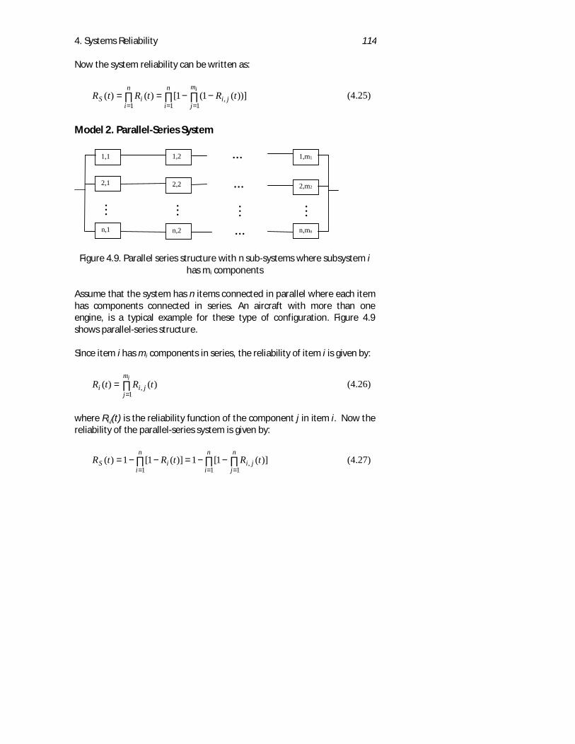
4. Systems Reliability 114
Now the system reliability can be written as:
∏ ∏∏= ==
−−==n
i
m
jji
n
iiS
itRtRtR
1 1,
1))](1(1[)()( (4.25)
Model 2. Parallel-Series System
Figure 4.9. Parallel series structure with n sub-systems where subsystem ihas mi components
Assume that the system has n items connected in parallel where each itemhas components connected in series. An aircraft with more than oneengine, is a typical example for these type of configuration. Figure 4.9shows parallel-series structure.
Since item i has mi components in series, the reliability of item i is given by:
∏=
=im
jjii tRtR
1, )()( (4.26)
where Ri,j(t) is the reliability function of the component j in item i. Now thereliability of the parallel-series system is given by:
∏ ∏∏= ==
−−=−−=n
i
n
jji
n
iiS tRtRtR
1 1,
1])(1[1)](1[1)( (4.27)
1,1
2,1
n,1
1,2
2,2
n,2
1,m1
2,m2
n,mn
......
......
4. Systems Reliability 115
4.25. REDUNDANT SYSTEMS
In systems, redundancy is a means of maintaining system integrity if
critical parts of it fail. In some cases this means replicating parts of the
system, in others, alternatives are used. A commercial aircraft has to be
able to complete a take-off and landing with one of its engines shutdown
but, except under very special circumstances, no such aircraft would be
allowed to leave the departure gate if any of its engines are not functioning.
And yet, ETOPS, extended twin engine operations allows certified twin-
engine aircraft (e.g. Boeing 777 and Airbus 330) to fly up to 180 minutes
from a suitable landing site. This is based on the probability that even if
one of the engines fails that far from land, the other is sufficiently, reliable
to make the probability of not reaching a landing site an acceptable risk. It
should be noted that in normal flight, i.e. at cruising speed and altitude, the
engines are generally doing very little work and usually are throttled back.
If an engine fails, it would normally be wind-milled to minimise 'parasitic'
drag but, even then, it still offers a considerable resistance and, of course,
produces an in-balance which has to be offset by the rudder and other
controllable surfaces all of which means the functional engine has to work
considerably harder thus increasing its probability of failure.
If the aircraft only had one engine and it failed, the probability of landingsafely with no engines is not very high, at least, for fast military jets. In

4. Systems Reliability 116
most cases ultimately, if the engine cannot be re-lit, the only option is toeject after directing the aircraft away from inhabited areas, if there is time.With commercial airlines, neither the pilot, the crew nor the passengershave the option of ejecting or baling out if the aircraft suffers a total enginefailure (i.e. all engines fail). These aircraft will glide, to a certain extend but,with no power, none of the instruments will function and, there will be nopower assistance for the control surfaces or to deploy the landing gear. Forthis reason, they are fitted with wind turbines that should drop down andstart functioning if there is prolonged loss of power. This gives the pilotssome control, but even then, large airliners are not going to rise on athermal, however good the pilot may be.
A Boeing 767, on one of its first flights, had a total engine failure some1500 miles from its intended destination, Ontario. All attempts to re-lightthe engines failed simply because it had run out of fuel. There was a totalblackout in the cockpit and, even when the co-pilot managed to find a torch(flashlights) all this showed was that none of the instruments were working(being all digital and computer controlled). The pilot, by pure chance,happened to be an extremely accomplished glider pilot and, again by purechance, the co-pilot happened to be particularly familiar with this part ofCanada, some 200 miles outside Winnipeg. For several minutes the pilotmanhandled the controls and managed to stop the aircraft from loosingheight too quickly. Eventually the wind turbine deployed which gave themenough power for the instruments, radio and power assisted controls towork again. Unfortunately the aircraft had lost too much height to reachWinnipeg but, it had just enough to get to an ex-military runway (used as astrip for drag racing). There was just enough power to lock the mainundercarriage down, but not the nose wheel. The Gimli Glider as it becameknown, landed safely with no serious casualties. But, out of eleven otherpilots, who later tried to land the aircraft in the same circumstances on aflight simulator all crashed. Had it not been for the 'redundant' windturbine, it is almost certain even this experienced glider pilot would havecrashed killing all on board.
If the Boeing 777, say, was fitted with three or four Rolls-Royce Trent800s, Pratt & Whitney 4084s or General Electric GE 90's (instead of the twoit currently has) then there would be true redundancy since it needs onlytwo to achieve ETOPS (Extended Twin-engine Operations). There are,however, a number of problems with this design. Firstly, it would add verysignificantly to both weight and drag, to the point where it would seriouslyreduce the payload and range, probably making the aircraft uneconomicalto operate and hence undesirable to the airlines. Secondly such an increasein weight and drag would probably mean the normal two engines would
4. Systems Reliability 117
provide insufficient thrust therefore either more powerful engines wouldbe needed or, the extra engines would have to be used rendering them nolonger truly redundant.
On the Boeing 767, for example, the IFSD (In Flight Shut Down) rateafter 10 million hours was less than 0.02 per thousand flying hours (thestandard measure in the aerospace industry). And, none of these had ledto the loss of a single life, let alone an aircraft with its full complement ofpassengers and crew. It is quite likely that, in some of the instances, flightswould have been diverted from their scheduled destinations to alternatives,for safety reasons. The inconvenience to passengers (and airlines) wouldhave cost the airline but, the amount would, almost certainly, have beensignificantly less than the loss of revenue resulting from the reducedpayload had truly redundant engines been fitted.In many cases, the redundant items may not be functioning simultaneouslyas in the case of parallel or r-out-of-n configurations. The redundant itemswill be turned on only when the main item fails. In some cases, the itemsmay be functioning simultaneously but one of them may be sharing muchhigher load compared to the other. Such types of systems are calledstandby redundant systems. Whenever the main item fails, a built-in switchsenses the failure and switches on the first standby item. It is importantthat the switch has to maintain its function. Failure of the switch can causethe system failure. The standby redundant systems are normally classifiedas cold standby, warm standby and hot standby.
Cold Standby System
In a cold standby, the redundant part of the system is switched on onlywhen the main part fails. For example, to meet the constantly changingdemand for electricity from the 'National Grid' it is necessary to keep anumber of steam turbines ready to come on stream whenever there is asurge in demand. The failure of a generator would result in instantaneousreduction in capacity, which would be rectified by bringing one of these'redundant' turbines up to full power. In the event of a power cut to ahospital, batteries may switch in instantly to provide emergency lightingand keep emergency equipment, e.g. respirators and monitors running.Petrol and diesel generators would then be started up to relieve thebatteries and provide additional power.
In a cold standby system, a redundant item is switched on only when theoperating item fails. That is, initially one item will be operating and whenthis item fails, one item from the redundant items will be switched on to
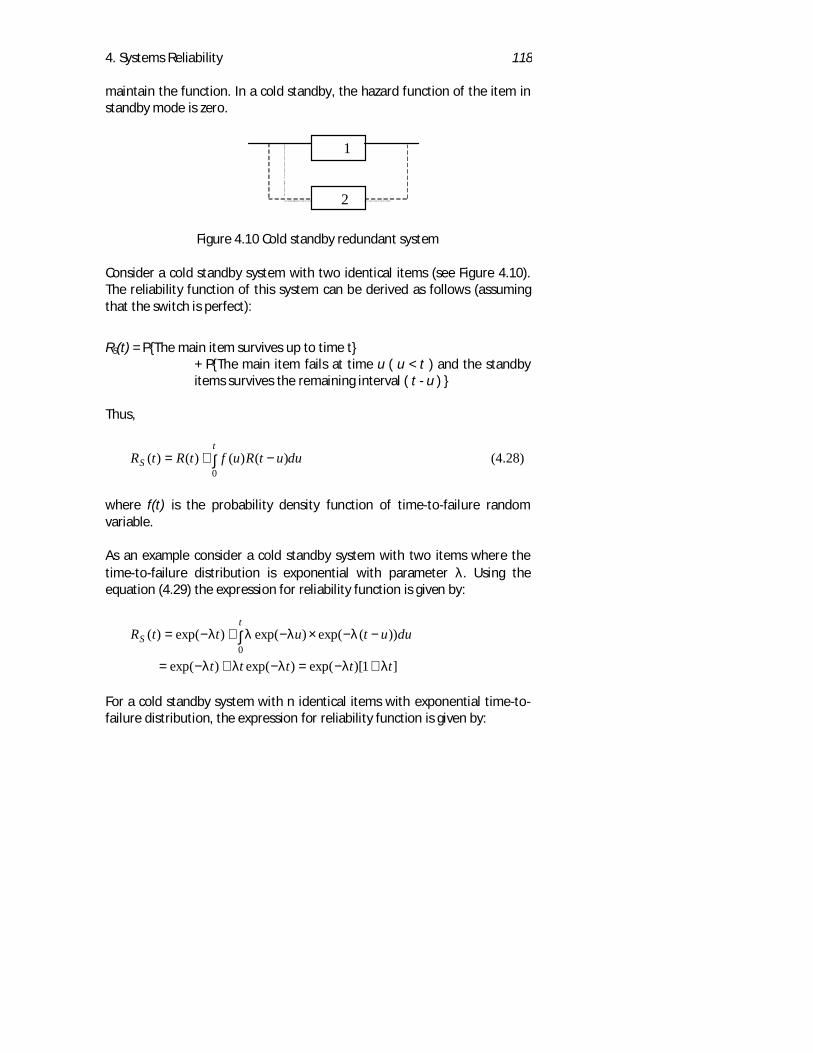
4. Systems Reliability 118
maintain the function. In a cold standby, the hazard function of the item instandby mode is zero.
Figure 4.10 Cold standby redundant system
Consider a cold standby system with two identical items (see Figure 4.10).The reliability function of this system can be derived as follows (assumingthat the switch is perfect):
RS(t) = P{The main item survives up to time t}+ P{The main item fails at time u ( u < t ) and the standbyitems survives the remaining interval ( t - u ) }
Thus,
duutRuftRtRt
S ∫ −+=0
)()()()( (4.28)
where f(t) is the probability density function of time-to-failure randomvariable.
As an example consider a cold standby system with two items where thetime-to-failure distribution is exponential with parameter λ. Using theequation (4.29) the expression for reliability function is given by:
]1)[exp()exp()exp(
))(exp()exp()exp()(0
ttttt
duututtRt
S
λλλλλ
λλλλ
+−=−+−=
−−×−+−= ∫
For a cold standby system with n identical items with exponential time-to-failure distribution, the expression for reliability function is given by:
1
2
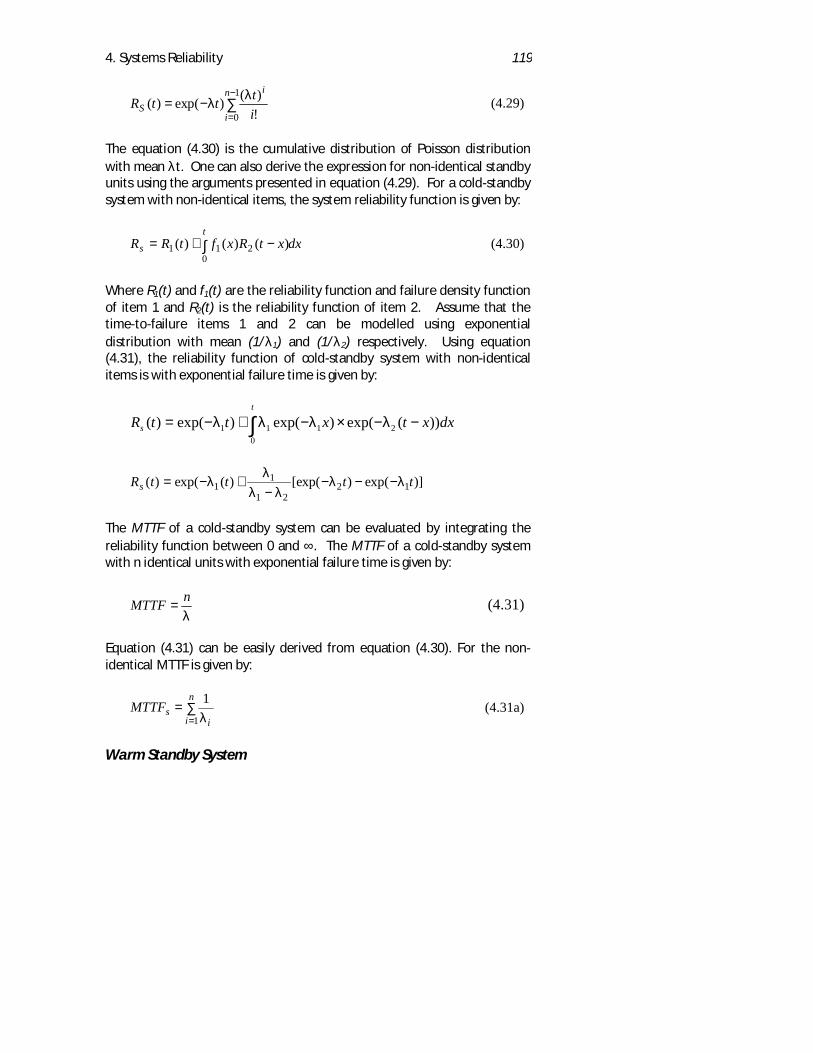
4. Systems Reliability 119
∑−
=−=
1
0 !)()exp()(
n
i
i
S itttR λ
λ (4.29)
The equation (4.30) is the cumulative distribution of Poisson distributionwith mean λt. One can also derive the expression for non-identical standbyunits using the arguments presented in equation (4.29). For a cold-standbysystem with non-identical items, the system reliability function is given by:
dxxtRxftRRt
s ∫ −+=0
211 )()()( (4.30)
Where R1(t) and f1(t) are the reliability function and failure density functionof item 1 and R2(t) is the reliability function of item 2. Assume that thetime-to-failure items 1 and 2 can be modelled using exponentialdistribution with mean (1/λ1) and (1/λ2) respectively. Using equation(4.31), the reliability function of cold-standby system with non-identicalitems is with exponential failure time is given by:
∫ −−×−+−=t
s dxxtxttR0
2111 ))(exp()exp()exp()( λλλλ
)]exp()[exp()(exp()( 1221
11 ttttRs λλ
λλλ
λ −−−−
+−=
The MTTF of a cold-standby system can be evaluated by integrating thereliability function between 0 and ∞. The MTTF of a cold-standby systemwith n identical units with exponential failure time is given by:
λnMTTF = (4.31)
Equation (4.31) can be easily derived from equation (4.30). For the non-identical MTTF is given by:
∑==
n
i isMTTF
1
1λ
(4.31a)
Warm Standby System
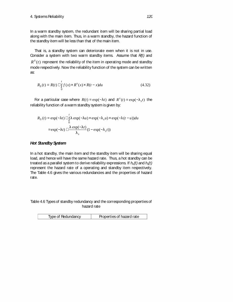
4. Systems Reliability 120
In a warm standby system, the redundant item will be sharing partial loadalong with the main item. Thus, in a warm standby, the hazard function ofthe standby item will be less than that of the main item.
That is, a standby system can deteriorate even when it is not in use.Consider a system with two warm standby items. Assume that R(t) and
R ts ( ) represent the reliability of the item in operating mode and standbymode respectively. Now the reliability function of the system can be writtenas:
duxtRxRxftRtRt
sS ∫ −××+=
0)()()()()( (4.32)
For a particular case where )exp()( ttR λ−= and )exp()( ttR ss λ−= the
reliability function of a warm standby system is given by:
))exp(1()exp()exp(
))(exp()exp()exp()exp()(0
ttt
duutuuttR
ss
t
sS
λλ
λλλ
λλλλλ
−−−
+−=
−−×−×−+−= ∫
Hot Standby System
In a hot standby, the main item and the standby item will be sharing equalload, and hence will have the same hazard rate. Thus, a hot standby can betreated as a parallel system to derive reliability expressions. If ho(t) and hs(t)represent the hazard rate of a operating and standby item respectively.The Table 4.6 gives the various redundancies and the properties of hazardrate.
Table 4.6 Types of standby redundancy and the corresponding properties ofhazard rate
Type of Redundancy Properties of hazard rate
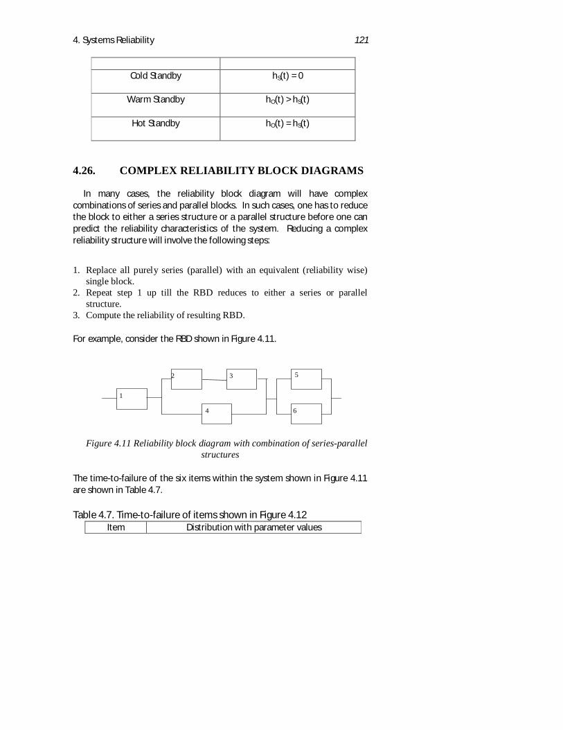
4. Systems Reliability 121
Cold Standby hS(t) = 0
Warm Standby hO(t) > hS(t)
Hot Standby hO(t) = hS(t)
4.26. COMPLEX RELIABILITY BLOCK DIAGRAMS
In many cases, the reliability block diagram will have complexcombinations of series and parallel blocks. In such cases, one has to reducethe block to either a series structure or a parallel structure before one canpredict the reliability characteristics of the system. Reducing a complexreliability structure will involve the following steps:
1. Replace all purely series (parallel) with an equivalent (reliability wise)single block.
2. Repeat step 1 up till the RBD reduces to either a series or parallelstructure.
3. Compute the reliability of resulting RBD.
For example, consider the RBD shown in Figure 4.11.
Figure 4.11 Reliability block diagram with combination of series-parallelstructures
The time-to-failure of the six items within the system shown in Figure 4.11are shown in Table 4.7.
Table 4.7. Time-to-failure of items shown in Figure 4.12Item Distribution with parameter values
2 3
4
5
6
1
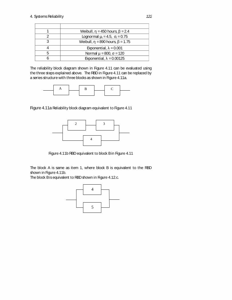
4. Systems Reliability 122
1 Weibull, η = 450 hours, β = 2.42 Lognormal µl = 4.5, σl = 0.753 Weibull, η = 890 hours, β = 1.75
4 Exponential, λ = 0.0015 Normal µ = 800, σ = 1206 Exponential, λ = 0.00125
The reliability block diagram shown in Figure 4.11 can be evaluated usingthe three steps explained above. The RBD in Figure 4.11 can be replaced bya series structure with three blocks as shown in Figure 4.11a.
Figure 4.11a Reliability block diagram equivalent to Figure 4.11
Figure 4.11b RBD equivalent to block B in Figure 4.11
The block A is same as item 1, where block B is equivalent to the RBDshown in Figure 4.11b.The block B is equivalent to RBD shown in Figure 4.12.c.
A B C
2 3
4
4
5
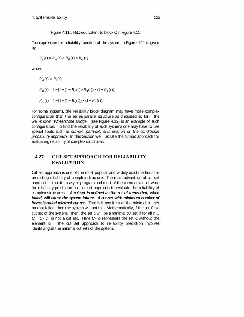
4. Systems Reliability 123
Figure 4.11c. RBD equivalent to block C in Figure 4.11
The expression for reliability function of the system in Figure 4.11 is givenby:
)()()()( tRtRtRtR CBAs ××=
where
)()( 1 tRtRA =
))](1())()(1(1[1)( 432 tRtRtRtRB −××−−−=
))](1())(1(1[1)( 65 tRtRtRC −×−−−=
For some systems, the reliability block diagram may have more complexconfiguration than the series/parallel structure as discussed so far. Thewell-known ‘Wheatstone Bridge’ (see Figure 4.12) is an example of suchconfiguration. To find the reliability of such systems one may have to usespecial tools such as cut-set, path-set, enumeration or the conditionalprobability approach. In this Section we illustrate the cut-set approach forevaluating reliability of complex structures.
4.27. CUT SET APPROACH FOR RELIABILITYEVALUATION
Cut-set approach is one of the most popular and widely used methods forpredicting reliability of complex structure. The main advantage of cut-setapproach is that it is easy to program and most of the commercial softwarefor reliability prediction use cut-set approach to evaluate the reliability ofcomplex structures. A cut-set is defined as the set of items that, whenfailed, will cause the system failure. A cut-set with minimum number ofitems is called minimal cut set. That is if any item of the minimal cut sethas not failed, then the system will not fail. Mathematically, if the set C is acut set of the system. Then, the set C will be a minimal cut set if for all ci ∈C, C - ci is not a cut set. Here C - ci represents the set C without theelement ci. The cut set approach to reliability prediction involvesidentifying all the minimal cut sets of the system.
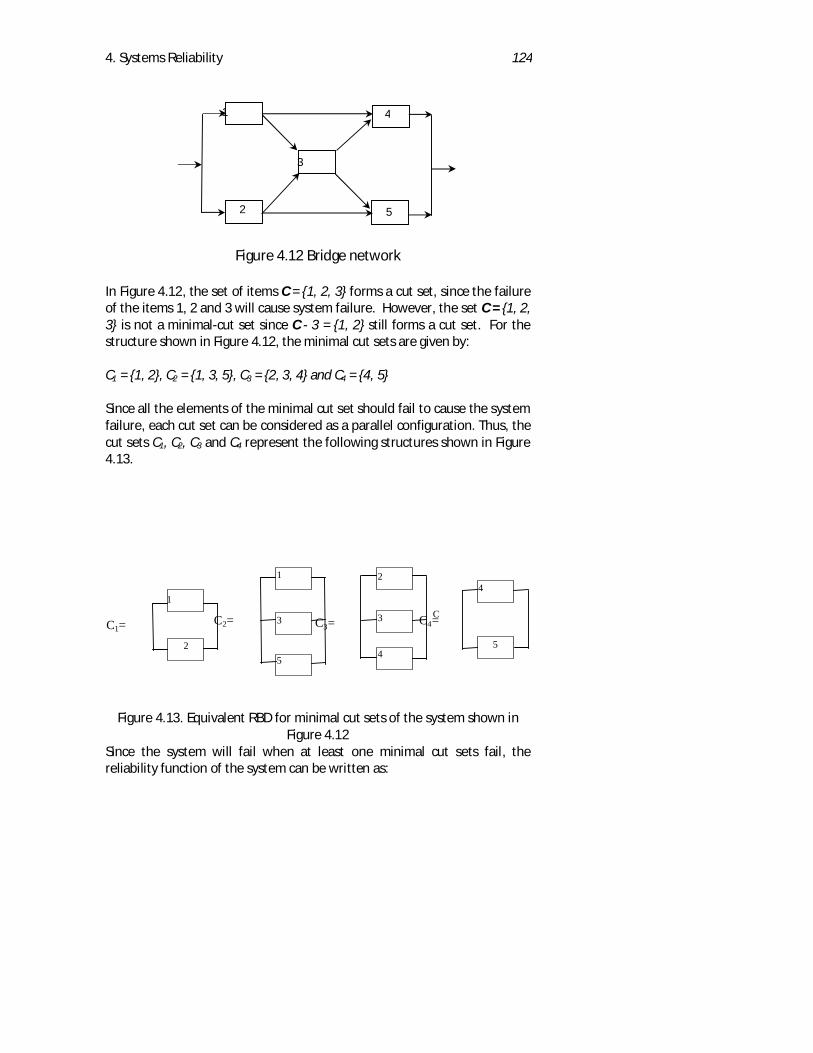
4. Systems Reliability 124
Figure 4.12 Bridge network
In Figure 4.12, the set of items C = {1, 2, 3} forms a cut set, since the failureof the items 1, 2 and 3 will cause system failure. However, the set C = {1, 2,3} is not a minimal-cut set since C - 3 = {1, 2} still forms a cut set. For thestructure shown in Figure 4.12, the minimal cut sets are given by:
C1 = {1, 2}, C2 = {1, 3, 5}, C3 = {2, 3, 4} and C4 = {4, 5}
Since all the elements of the minimal cut set should fail to cause the systemfailure, each cut set can be considered as a parallel configuration. Thus, thecut sets C1, C2, C3 and C4 represent the following structures shown in Figure4.13.
Figure 4.13. Equivalent RBD for minimal cut sets of the system shown inFigure 4.12
Since the system will fail when at least one minimal cut sets fail, thereliability function of the system can be written as:
5
1
2
3
4
1
2
1
5
3
2
3
4
4
5
C1=CC2= C4=C3=
4. Systems Reliability 125
RS(t) = RC1(t) × RC2(t) × RC3(t) × RC4(t) (4.33)
where RC1 (t), RC2 (t), RC3(t) and RC4(t) are the reliability function of thestructures represented by the cut sets C1, C2, C3 and C4 respectively. If Ri(t)denote the failure function of the items 1, 2, 3, 4 and 5, then we have:
)()(1)(),()()(1)()()()(1)(),()(1)(
5444323
5312211
tFtFtRCtFtFtFtRCtFtFtFtRCtFtFtRC
−=−=−=−=
Substituting the above expressions in equation (4.34), we get the failurefunction for the complex structure shown in Figure 4.12.
In general, cut set approach involves the following steps:
1. Identify all the minimal cut sets of the system.2. Since all the elements of the minimal cut set should fail to cause the
system failure, each cut set can be treated as a parallel configuration.3. Since failure of any one minimal cut set can cause system failure,
different minimal cut sets can be treated as a series configuration.
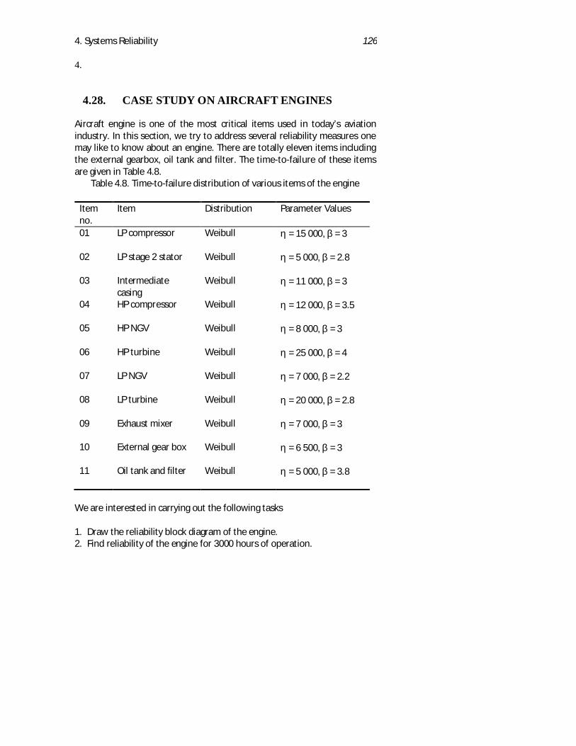
4. Systems Reliability 126
4.
4.28. CASE STUDY ON AIRCRAFT ENGINES
Aircraft engine is one of the most critical items used in today’s aviationindustry. In this section, we try to address several reliability measures onemay like to know about an engine. There are totally eleven items includingthe external gearbox, oil tank and filter. The time-to-failure of these itemsare given in Table 4.8.
Table 4.8. Time-to-failure distribution of various items of the engine
Itemno.
Item Distribution Parameter Values
01 LP compressor Weibull η = 15 000, β = 3
02 LP stage 2 stator Weibull η = 5 000, β = 2.8
03 Intermediatecasing
Weibull η = 11 000, β = 3
04 HP compressor Weibull η = 12 000, β = 3.5
05 HP NGV Weibull η = 8 000, β = 3
06 HP turbine Weibull η = 25 000, β = 4
07 LP NGV Weibull η = 7 000, β = 2.2
08 LP turbine Weibull η = 20 000, β = 2.8
09 Exhaust mixer Weibull η = 7 000, β = 3
10 External gear box Weibull η = 6 500, β = 3
11 Oil tank and filter Weibull η = 5 000, β = 3.8
We are interested in carrying out the following tasks
1. Draw the reliability block diagram of the engine.2. Find reliability of the engine for 3000 hours of operation.
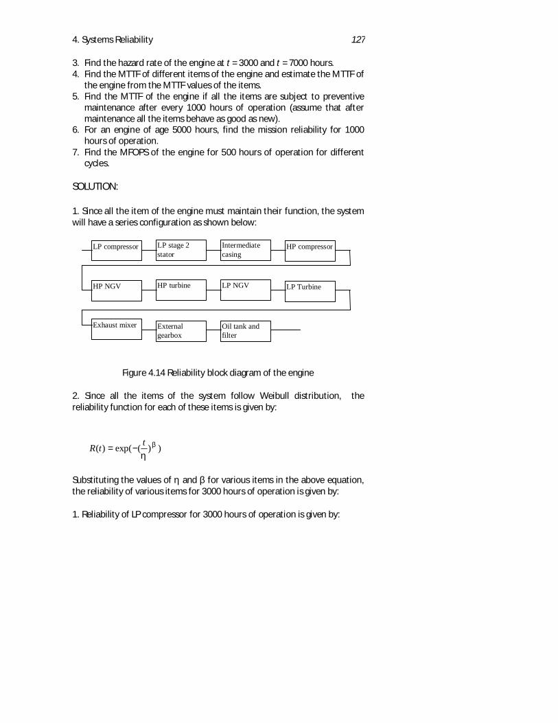
4. Systems Reliability 127
3. Find the hazard rate of the engine at t = 3000 and t = 7000 hours.4. Find the MTTF of different items of the engine and estimate the MTTF of
the engine from the MTTF values of the items.5. Find the MTTF of the engine if all the items are subject to preventive
maintenance after every 1000 hours of operation (assume that aftermaintenance all the items behave as good as new).
6. For an engine of age 5000 hours, find the mission reliability for 1000hours of operation.
7. Find the MFOPS of the engine for 500 hours of operation for differentcycles.
SOLUTION:
1. Since all the item of the engine must maintain their function, the systemwill have a series configuration as shown below:
Figure 4.14 Reliability block diagram of the engine
2. Since all the items of the system follow Weibull distribution, thereliability function for each of these items is given by:
))(exp()( β
ηttR −=
Substituting the values of η and β for various items in the above equation,the reliability of various items for 3000 hours of operation is given by:
1. Reliability of LP compressor for 3000 hours of operation is given by:
LP compressor LP stage 2stator
Intermediatecasing
HP compressor
HP NGV HP turbine LP NGV LP Turbine
Exhaust mixer Externalgearbox
Oil tank andfilter
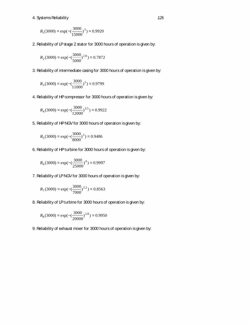
4. Systems Reliability 128
9920.0))150003000(exp()3000( 3
1 =−=R
2. Reliability of LP stage 2 stator for 3000 hours of operation is given by:
7872.0))50003000(exp()3000( 8.2
2 =−=R
3. Reliability of intermediate casing for 3000 hours of operation is given by:
9799.0))110003000(exp()3000( 3
3 =−=R
4. Reliability of HP compressor for 3000 hours of operation is given by:
9922.0))120003000(exp()3000( 5.3
4 =−=R
5. Reliability of HP NGV for 3000 hours of operation is given by:
9486.0))80003000(exp()3000( 3
5 =−=R
6. Reliability of HP turbine for 3000 hours of operation is given by:
9997.0))250003000(exp()3000( 4
6 =−=R
7. Reliability of LP NGV for 3000 hours of operation is given by:
8563.0))70003000(exp()3000( 2.2
7 =−=R
8. Reliability of LP turbine for 3000 hours of operation is given by:
9950.0))200003000(exp()3000( 8.2
8 =−=R
9. Reliability of exhaust mixer for 3000 hours of operation is given by:
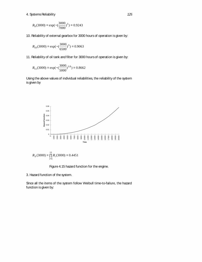
4. Systems Reliability 129
9243.0))70003000(exp()3000( 3
9 =−=R
10. Reliability of external gearbox for 3000 hours of operation is given by:
9063.0))65003000(exp()3000( 3
10 =−=R
11. Reliability of oil tank and filter for 3000 hours of operation is given by:
8662.0))50003000(exp()3000( 8.3
11 =−=R
Using the above values of individual reliabilities, the reliability of the systemis given by
4451.0)3000()3000(11
1== ∏
=iiS RR
Figure 4.15 hazard function for the engine.
3. Hazard function of the system.
Since all the items of the system follow Weibull time-to-failure, the hazardfunction is given by:
0
0.01
0.02
0.03
0.04
0.05
0.06
0
1000
2000
3000
4000
5000
6000
7000
8000
9000
1000
0
1100
0
1200
0
1300
0
1400
0
1500
0
1600
0
1700
0
1800
0
1900
0
2000
0
Time
Haz
ard
func
tion
4. Systems Reliability 130
1))(()( −= β
ηηβ tth
The system hazard function is given by:
∑=
=11
1)()(
iiS thth
It is easy to verify that the hazard function of the system at t = 3000 and t=7000 is given by:
000791.0)3000( =Sh and 004796.0)7000( =Sh
Figure 4.15 depicts the hazard function for the engine.
4. The expression for MTTF is given by:
)11(β
η +Γ×=MTTF
By substituting the values of η and β, one can find the MTTF of differentitems. Table 4.9 gives the MTTF of different items.
Table 4.9 MTTF of different item of the engine
Item MTTF (in hours)
LP compressor 13 395
LP stage 2 stator 4 450
Intermediate casing 9 823
HP compressor 10 800
HP NGV 7 144
HP turbine 22 650
4. Systems Reliability 131
LP NGV 6 202
LP turbine 17 800
Exhaust mixer 6 251
External gear box 5 804
Oil tank and filter 4 525
Since the lowest MTTF is 4 450 (LP stage 2 stator), the MTTF of engine willbe less than 4 450.
5. Mean time to failure of a system subject to preventive maintenance isgiven by:
)(1
)(0
PS
T
S
pm TR
dttRMTTF
P
−=
∫
It is given that the engine is subject to preventive maintenance every 1000hours of operation. Thus, TP = 1000 hours. The above expression can beevaluated using numerical integration. The approximate values of MTTFpm
is:
075,270369.0
06.999)1000(1
)(1000
0 ≈≈−
=∫
S
S
pm R
dttRMTTF
6. The mission reliability of the engine is given by:
)(),(),(
b
mbmb tR
ttRttMR =
where tb is the age of the item at the beginning of the mission and tm is themission duration. Substituting tb = 5000 and tm = 1000, we have
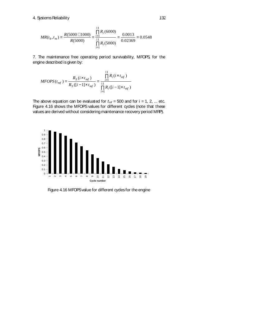
4. Systems Reliability 132
0548.002369.00013.0
)5000(
)6000(
)5000()10005000(),( 11
1
11
1 ===+
=∏
∏
=
=
ii
ii
mbR
R
RRttMR
7. The maintenance free operating period survivability, MFOPS, for theengine described is given by:
∏
∏
=
=
×−
×=
×−
×= 11
1
11
1
)]1([
)(
)]1([)(
)(
imfi
imfi
mfS
mfSmf
tiR
tiR
tiRtiR
tMFOPS
The above equation can be evaluated for tmf = 500 and for i = 1, 2, ... etc.Figure 4.16 shows the MFOPS values for different cycles (note that thesevalues are derived without considering maintenance recovery period MRP).
Figure 4.16 MFOPS value for different cycles for the engine
0
0.1
0.2
0.3
0.4
0.5
0.6
0.7
0.8
0.9
1
1 2 3 4 5 6 7 8 9 10 11 12 13 14 15 16 17 18 19
Cycle number
MFO
PS
5. Maintainability and Maintenance 133
Chapter 5
Maintainability and MaintenanceMaintenance is the management of failures and
the assurance of availability
J Hessburg
Maintainability and maintenance has always been important to the industryas it affects the performance as well as the finance. For commercialairlines, maintenance costs around 10% of the airlines total cost, as much asfuel and travel agents' commission (M Lam, 1995). Operators/users wouldlike their system to be available and safe to operate when required. Oneshould be lucky to find a smiling customer when the system fails and ittakes a long time to recover the functionality.There are several ways that designers can provide maximum utility of theirproduct. One way is to build items/systems that are extremely reliable (andconsequently will, almost certainly, have a higher acquisition cost). Anotheris to design systems that are quick and easy to repair when they fail.Obviously, the main objective of the designer is to provide a reliable andsafe item at an affordable price.Maintenance is the action necessary to sustain and restore theperformance, reliability and safety of the item. The main objective ofmaintenance is to assure the availability of the system for use whenrequired. For aircraft, maintenance forms an essential part ofairworthiness. The common objective of aircraft maintenance, civil ormilitary, is to provide a fully serviceable aircraft when it is required by theoperator at minimum cost (Knotts, 1996). However, maintenance costsmoney. The annual maintenance cost of production assets in the UnitedKingdom is estimated in excess of $13 billion, with $2 billion wastedthrough inefficient maintenance management practices (Knotts, 1999).
5. Maintainability and Maintenance 134
Maintenance also accounts for approximately 10% of the organisations’employees and at least 10-15% of its operating costs.
29. CONCEPT OF MAINTAINABILITY
In the previous chapters, we showed that it is important for theoperator/user to know the reliability characteristics of the item. We alsorecognised that it is almost impossible for any item to maintain its functionforever, as failure and the degradation of performance is inevitable. Thus,for the user it is equally, or even more important to know:
• When and how often maintenance tasks should be performed• How they should be performed• How many people will be needed• What skills they will need and how much training• How much the restoration will cost• How long the system will be down• What facilities and equipment (special and general) will be required.
All the above information is important as it affects the availability and thelife cycle cost of the system. One has to apply a scientific discipline to findanswers to these questions.Maintainability is the scientific discipline that studies complexity, factorsand resources related to the maintenance tasks needed to be performed bythe user in order to maintain the functionality of a system, and works outmethods for their quantification, assessment, prediction and improvement.Maintainability Engineering is rapidly growing in importance because itprovides a very powerful tool to engineers for the quantitative descriptionof the inherent ability of their system/product to be restored by performingspecified maintenance tasks. It also contributes towards the reduction ofmaintenance costs of a system during its utilisation to achieve optimum lifecycle cost.The maintainability engineering function involves the formulation of anacceptable combination of design features, which directly affectmaintenance and system support requirements, repair policies, andmaintenance resources. Some physical design features such as accessibility,visibility, testability, complexity and interchangeability affect the speed andease with which maintenance can be performed.

5. Maintainability and Maintenance 135
Maintainability studies have the following objectives (R Knotts 1996):
To guide and direct design decisionsTo predict quantitative maintainability characteristics of a systemTo identify changes to a system's design needed to meet operationalrequirements
In the technical literature, several definitions for maintainability can befound. For example, the US Department of Defence's MIL-STD-721C (1966)defines maintainability as:
The measure of the ability of an item to be retained in or restored tospecified condition when maintenance is performed by personnelhaving specified skill levels, using prescribed procedures andresources, at each prescribed level of maintenance and repair.
Maintainability can be expressed in terms of maintenance frequencyfactors, maintenance elapsed times and maintenance cost.Maintainability therefore is an inherent design characteristic dealingwith the ease, accuracy, safety, and economy in the performance ofmaintenance functions. Maintainability requirements are defined inconceptual design as part of system operational requirements andthe maintenance concept. Anon (1992) describes maintainability as:
The characteristic of material design and installation thatdetermines the requirements for maintenance expendituresincluding time, manpower, personnel skill, test equipment,technical data and facilities to accomplish operational objectives inthe user's operational environment.
One of the common misperceptions is that maintainability is simply theability to reach a component to perform the required maintenance task(accessibility). Of course, accessibility is one of the main concerns for manymaintenance engineers. Figure 5.1 illustrates an accessibility problem inone of the older twin-engine fighter aircraft, Gloster Javelin. Before anengine could be changed, the jet pipe had to be disconnected andremoved. To remove the jet pipe it was necessary for a technician togain access through a hatch and then be suspended upside down toreach the clamps and pipes which had to be disconnected. The job
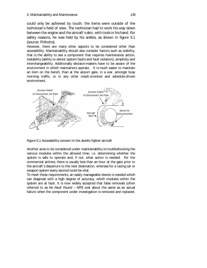
5. Maintainability and Maintenance 136
could only be achieved by touch; the items were outside of thetechnician’s field of view. The technician had to work his way downbetween the engine and the aircraft’s skin, with tools in his hand. Forsafety reasons, he was held by his ankles, as shown in figure 5.1(source: R Knotts).However, there are many other aspects to be considered other thanaccessibility. Maintainability should also consider factors such as visibility,that is the ability to see a component that requires maintenance action,testability (ability to detect system faults and fault isolation), simplicity andinterchangeability. Additionally decision-makers have to be aware of theenvironment in which maintainers operate. It is much easier to maintainan item on the bench, than at the airport gate, in a war, amongst busymorning traffic, or in any other result-oriented and schedule-drivenenvironment.
Figure 5.1 Accessibility concern in the Javelin fighter aircraft
Another area to be considered under maintainability is troubleshooting thevarious modules within the allowed time, i.e. determining whether thesystem is safe to operate and, if not, what action is needed. For thecommercial airlines, there is usually less than an hour at the gate prior tothe aircraft’s departure to the next destination, whereas for a racing car orweapon system every second could be vital.To meet these requirements, an easily manageable device is needed whichcan diagnose with a high degree of accuracy, which modules within thesystem are at fault. It is now widely accepted that false removals (oftenreferred to as No Fault Found – NFF) cost about the same as an actualfailure when the component under investigation is removed and replaced.
Access Hatchto Disconnect Jet Pipe
Items forDisconnection
Access Hatchto Disconnect Jet Pipe
AircraftSkin
5. Maintainability and Maintenance 137
Reducing the number of false removals, therefore, would be a big costsaver.Devices with these capabilities have been developed in the aerospace,Formula 1 racing car and luxury car industries. For example, the Boeing 777includes an 'on-board maintenance system' with the objective to assist theairlines to avoid expensive gate delays and flight cancellations. For similarpurposes the Flight Control Division of the Wright Laboratory in the USA hasdeveloped a fault detection/isolation system for F-16 aircraft, which allowsmaintainers, novice as well as expert, to find failed components. In the next section, we discuss the maintainability measures and how thesemeasures can be used for effective maintenance management.
30. MEASURES OF MAINTAINABILITY
It is extremely important for the user to have information about thefunctionality, cost, safety, and other characteristics of the product underconsideration at the beginning of its operating life. However, it is equally,or even more important to have information about the characteristics withwhich to define the maintenance time. Measures of maintainability arerelated to the ease and economy of maintenance such as; elapsed time thatan item spends in the state of failure, man-hours required completing amaintenance task, frequency of maintenance, and the cost of maintenance.As the elapsed time has a significant influence on the availability of thesystem, operators would like to know the maintenance times; not just themean time but also the probability that a maintenance task will becompleted within a given time. Maintenance elapsed times are evenadvertised as a marketing strategy.
30.1 Maintenance Elapsed-Time
The length of the elapsed time, required for the restoration of functionality,called time to restore, is largely determined at an early stage of the designphase. The maintenance elapsed time is influenced by the complexity of themaintenance task, accessibility of the items, safety of the restoration,testability, physical location of the item, as well as the decisions related tothe requirements for the maintenance support resources (facilities, spares,tools, trained personnel, etc). It is therefore a function of themaintainability and supportability of the system. It will, of course, also beinfluenced by other factors during the various stages of the life of thesystem but any bad decision made (either explicitly or by default) during
5. Maintainability and Maintenance 138
the design stage will be costly to rectify at a later stage and will significantlyaffect both the operational costs and system availability.
1. Personnel factors which represent the influence of the skill, motivation,experience, attitude, physical ability, self-discipline, training,responsibility and other similar characteristics related to the personnelinvolved;
2. Conditional factors which represent the influence of the operatingenvironment and the consequences of failure with the physical condition,geometry, and shape of the item under restoration;
3. Environmental factors which represent the influence of factors such astemperature, humidity, noise, lighting, vibration, time of the day, time ofthe year, wind, noise, and others such as those similar to the maintenancepersonnel factors during restoration.
This maintainability measure can be represented using the probability thatthe maintenance task considered will be completed by a stated time. Sincethe maintenance elapsed time is a random variable, one can use thecumulative distribution function of the elapsed time to find the percentageof maintenance tasks that will be completed within a specified time.
Mean Time to Repair
One approach for measuring maintainability is through Mean Time toRepair (MTTR). MTTR is the expected value of the item's repair time. Withthe knowledge of the reliability and maintainability of the sub-systems onecan evaluate the maintainability of the system, that is, mean time to repairof the system, MTTRs (Birolini, 1994).Assume that the reliability block diagram of the system has a seriesstructure with n items with no redundancy. Let MTTFi and MTTRi be themean time to failure and mean time to repair of sub-system i in the system.Consider an arbitrarily large operating time T. Assuming that the failurerate of the unit is constant, the expected number of failures of unit i induring T is given by:
iMTTFT
(5.1)
The mean of total repair time to repair unit i during T is given by:
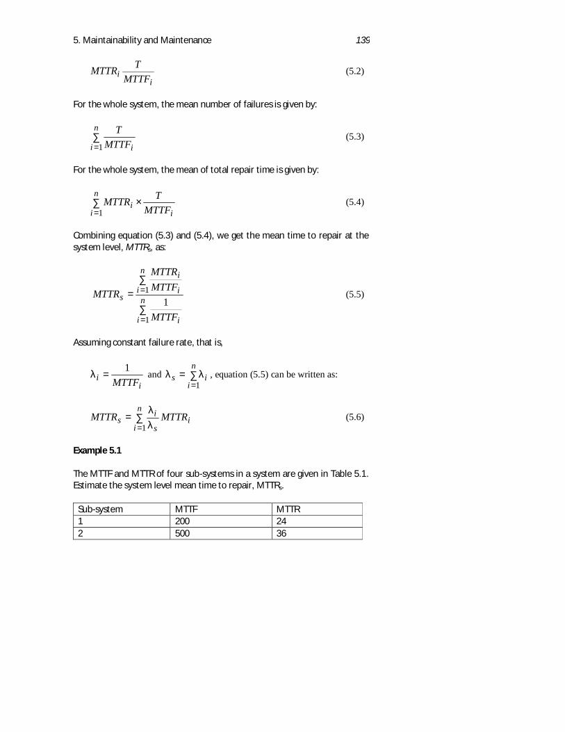
5. Maintainability and Maintenance 139
ii MTTF
TMTTR (5.2)
For the whole system, the mean number of failures is given by:
∑=
n
i iMTTFT
1(5.3)
For the whole system, the mean of total repair time is given by:
∑ ×=
n
i ii MTTF
TMTTR1
(5.4)
Combining equation (5.3) and (5.4), we get the mean time to repair at thesystem level, MTTRs, as:
∑
∑=
=
=n
i i
n
i i
i
s
MTTF
MTTFMTTR
MTTR
1
11
(5.5)
Assuming constant failure rate, that is,
ii MTTF
1=λ and ∑=
=
n
iis
1λλ , equation (5.5) can be written as:
∑==
n
ii
s
is MTTRMTTR
1 λλ
(5.6)
Example 5.1
The MTTF and MTTR of four sub-systems in a system are given in Table 5.1.Estimate the system level mean time to repair, MTTRs.
Sub-system MTTF MTTR1 200 242 500 36
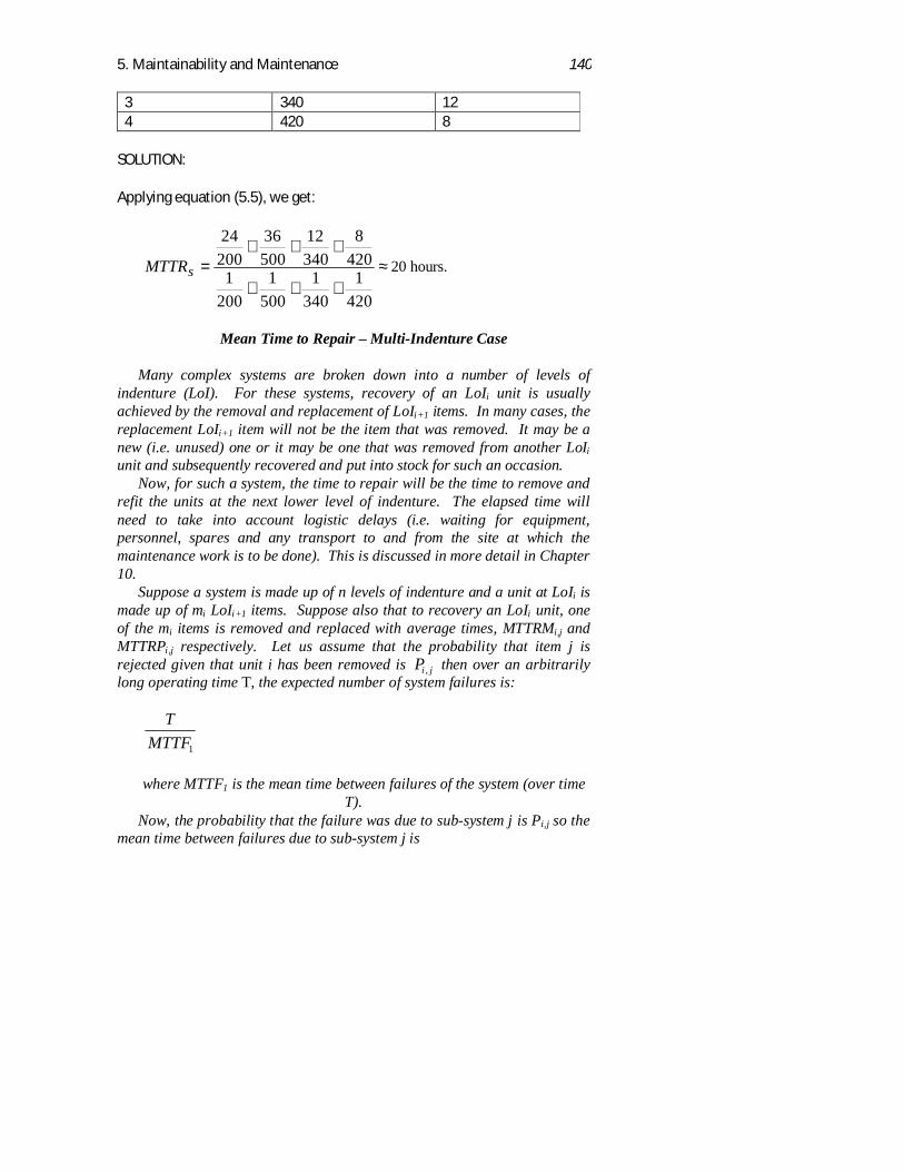
5. Maintainability and Maintenance 140
3 340 124 420 8
SOLUTION:
Applying equation (5.5), we get:
≈+++
+++=
4201
3401
5001
2001
4208
34012
50036
20024
sMTTR 20 hours.
Mean Time to Repair Multi-Indenture Case
Many complex systems are broken down into a number of levels ofindenture (LoI). For these systems, recovery of an LoIi unit is usuallyachieved by the removal and replacement of LoIi+1 items. In many cases, thereplacement LoIi+1 item will not be the item that was removed. It may be anew (i.e. unused) one or it may be one that was removed from another LoIiunit and subsequently recovered and put into stock for such an occasion.
Now, for such a system, the time to repair will be the time to remove andrefit the units at the next lower level of indenture. The elapsed time willneed to take into account logistic delays (i.e. waiting for equipment,personnel, spares and any transport to and from the site at which themaintenance work is to be done). This is discussed in more detail in Chapter10.
Suppose a system is made up of n levels of indenture and a unit at LoIi ismade up of mi LoIi+1 items. Suppose also that to recovery an LoIi unit, oneof the mi items is removed and replaced with average times, MTTRMi,j andMTTRPi ,j respectively. Let us assume that the probability that item j isrejected given that unit i has been removed is Pi j, then over an arbitrarilylong operating time T, the expected number of system failures is:
TMTTF1
where MTTF1 is the mean time between failures of the system (over timeT).
Now, the probability that the failure was due to sub-system j is Pi,j so themean time between failures due to sub-system j is
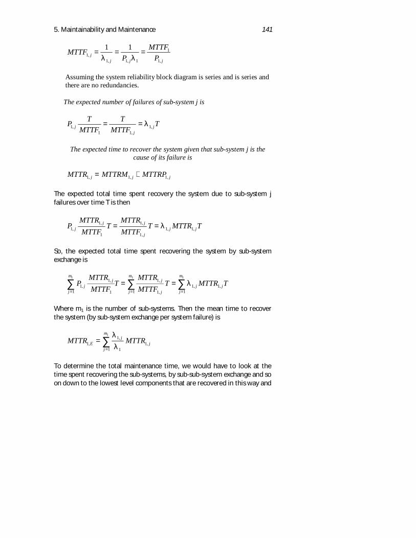
5. Maintainability and Maintenance 141
MTTFP
MTTFPj
j j j1
1 1 1
1
1
1 1,
, , ,
= = =λ λ
Assuming the system reliability block diagram is series and is series andthere are no redundancies.
The expected number of failures of sub-system j is
P TMTTF
TMTTF
Tjj
j11 1
1,,
,= = λ
The expected time to recover the system given that sub-system j is thecause of its failure is
MTTR MTTRM MTTRPj j j1 1 1, , ,= +
The expected total time spent recovery the system due to sub-system jfailures over time T is then
PMTTRMTTF
TMTTRMTTF
T MTTR Tjj j
jj j1
1
1
1
11 1,
, ,
,, ,= = λ
So, the expected total time spent recovering the system by sub-systemexchange is
PMTTRMTTF
TMTTRMTTF
T MTTR Tjj
j
mj
jj
m
j jj
m
11
11
1
111 1
1
1 1 1
,, ,
,, ,
= = =∑ ∑ ∑= = λ
Where m1 is the number of sub-systems. Then the mean time to recoverthe system (by sub-system exchange per system failure) is
MTTR MTTREj
jj
m
11
11
1
1
,,
,==
∑λλ
To determine the total maintenance time, we would have to look at thetime spent recovering the sub-systems, by sub-sub-system exchange and soon down to the lowest level components that are recovered in this way and
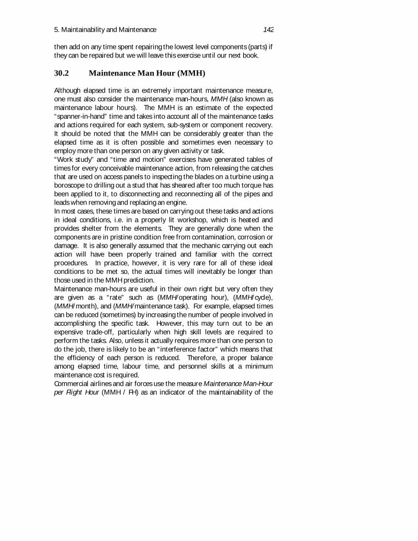
5. Maintainability and Maintenance 142
then add on any time spent repairing the lowest level components (parts) ifthey can be repaired but we will leave this exercise until our next book.
30.2 Maintenance Man Hour (MMH)
Although elapsed time is an extremely important maintenance measure,one must also consider the maintenance man-hours, MMH (also known asmaintenance labour hours). The MMH is an estimate of the expected“spanner-in-hand” time and takes into account all of the maintenance tasksand actions required for each system, sub-system or component recovery.It should be noted that the MMH can be considerably greater than theelapsed time as it is often possible and sometimes even necessary toemploy more than one person on any given activity or task.“Work study” and “time and motion” exercises have generated tables oftimes for every conceivable maintenance action, from releasing the catchesthat are used on access panels to inspecting the blades on a turbine using aboroscope to drilling out a stud that has sheared after too much torque hasbeen applied to it, to disconnecting and reconnecting all of the pipes andleads when removing and replacing an engine.In most cases, these times are based on carrying out these tasks and actionsin ideal conditions, i.e. in a properly lit workshop, which is heated andprovides shelter from the elements. They are generally done when thecomponents are in pristine condition free from contamination, corrosion ordamage. It is also generally assumed that the mechanic carrying out eachaction will have been properly trained and familiar with the correctprocedures. In practice, however, it is very rare for all of these idealconditions to be met so, the actual times will inevitably be longer thanthose used in the MMH prediction.Maintenance man-hours are useful in their own right but very often theyare given as a “rate” such as (MMH/operating hour), (MMH/cycle),(MMH/month), and (MMH/maintenance task). For example, elapsed timescan be reduced (sometimes) by increasing the number of people involved inaccomplishing the specific task. However, this may turn out to be anexpensive trade-off, particularly when high skill levels are required toperform the tasks. Also, unless it actually requires more than one person todo the job, there is likely to be an “interference factor” which means thatthe efficiency of each person is reduced. Therefore, a proper balanceamong elapsed time, labour time, and personnel skills at a minimummaintenance cost is required.Commercial airlines and air forces use the measure Maintenance Man-Hourper Flight Hour (MMH / FH) as an indicator of the maintainability of the
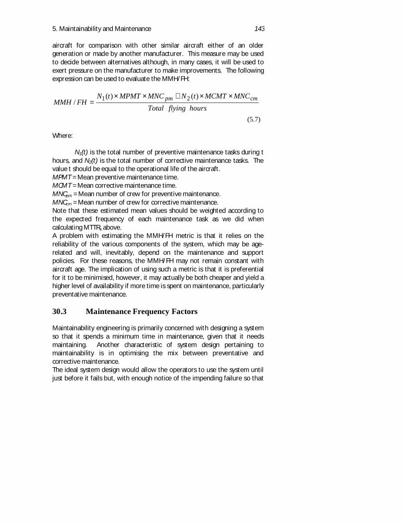
5. Maintainability and Maintenance 143
aircraft for comparison with other similar aircraft either of an oldergeneration or made by another manufacturer. This measure may be usedto decide between alternatives although, in many cases, it will be used toexert pressure on the manufacturer to make improvements. The followingexpression can be used to evaluate the MMH/FH:
hoursflyingTotalMNCMCMTtNMNCMPMTtN
FHMMH cmpm ××+××=
)()(/ 21
(5.7)
Where:
N1(t) is the total number of preventive maintenance tasks during thours, and N2(t) is the total number of corrective maintenance tasks. Thevalue t should be equal to the operational life of the aircraft.MPMT = Mean preventive maintenance time.MCMT = Mean corrective maintenance time.MNCpm = Mean number of crew for preventive maintenance.MNCcm = Mean number of crew for corrective maintenance.Note that these estimated mean values should be weighted according tothe expected frequency of each maintenance task as we did whencalculating MTTRs above.A problem with estimating the MMH/FH metric is that it relies on thereliability of the various components of the system, which may be age-related and will, inevitably, depend on the maintenance and supportpolicies. For these reasons, the MMH/FH may not remain constant withaircraft age. The implication of using such a metric is that it is preferentialfor it to be minimised, however, it may actually be both cheaper and yield ahigher level of availability if more time is spent on maintenance, particularlypreventative maintenance.
30.3 Maintenance Frequency Factors
Maintainability engineering is primarily concerned with designing a systemso that it spends a minimum time in maintenance, given that it needsmaintaining. Another characteristic of system design pertaining tomaintainability is in optimising the mix between preventative andcorrective maintenance.The ideal system design would allow the operators to use the system untiljust before it fails but, with enough notice of the impending failure so that
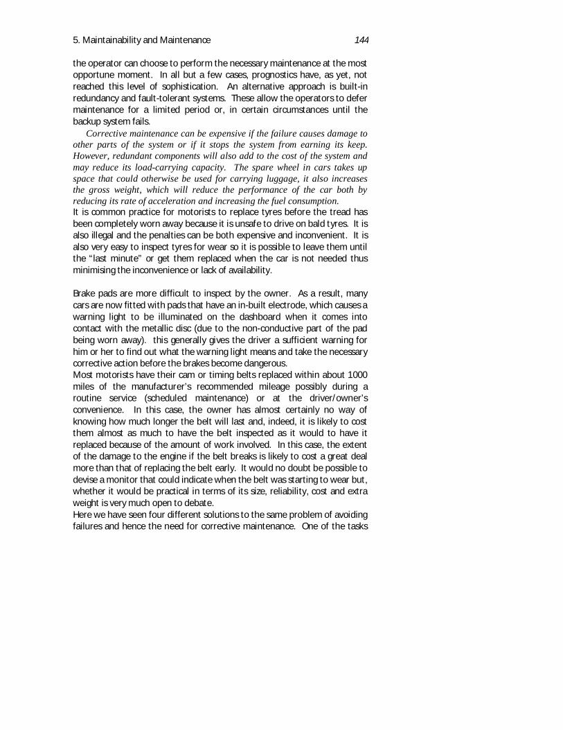
5. Maintainability and Maintenance 144
the operator can choose to perform the necessary maintenance at the mostopportune moment. In all but a few cases, prognostics have, as yet, notreached this level of sophistication. An alternative approach is built-inredundancy and fault-tolerant systems. These allow the operators to defermaintenance for a limited period or, in certain circumstances until thebackup system fails.
Corrective maintenance can be expensive if the failure causes damage toother parts of the system or if it stops the system from earning its keep.However, redundant components will also add to the cost of the system andmay reduce its load-carrying capacity. The spare wheel in cars takes upspace that could otherwise be used for carrying luggage, it also increasesthe gross weight, which will reduce the performance of the car both byreducing its rate of acceleration and increasing the fuel consumption.It is common practice for motorists to replace tyres before the tread hasbeen completely worn away because it is unsafe to drive on bald tyres. It isalso illegal and the penalties can be both expensive and inconvenient. It isalso very easy to inspect tyres for wear so it is possible to leave them untilthe “last minute” or get them replaced when the car is not needed thusminimising the inconvenience or lack of availability.
Brake pads are more difficult to inspect by the owner. As a result, manycars are now fitted with pads that have an in-built electrode, which causes awarning light to be illuminated on the dashboard when it comes intocontact with the metallic disc (due to the non-conductive part of the padbeing worn away). this generally gives the driver a sufficient warning forhim or her to find out what the warning light means and take the necessarycorrective action before the brakes become dangerous.Most motorists have their cam or timing belts replaced within about 1000miles of the manufacturer’s recommended mileage possibly during aroutine service (scheduled maintenance) or at the driver/owner’sconvenience. In this case, the owner has almost certainly no way ofknowing how much longer the belt will last and, indeed, it is likely to costthem almost as much to have the belt inspected as it would to have itreplaced because of the amount of work involved. In this case, the extentof the damage to the engine if the belt breaks is likely to cost a great dealmore than that of replacing the belt early. It would no doubt be possible todevise a monitor that could indicate when the belt was starting to wear but,whether it would be practical in terms of its size, reliability, cost and extraweight is very much open to debate.Here we have seen four different solutions to the same problem of avoidingfailures and hence the need for corrective maintenance. One of the tasks

5. Maintainability and Maintenance 145
of the maintainability engineer is to determine which, if any of these, orother similar approaches is appropriate taking into consideration the costsand practicalities in each circumstance.There is clearly a need to strike a balance. Preventative maintenance maycause components to be replaced unnecessarily (or at least prematurely).Allowing a system to run until it fails may maximise the times betweenmaintenance but failures can be expensive to rectify both because of theextent of the damage caused and because of the loss of availability of thesystem whilst it is being maintained. Prognostics can help but these toohave their own problems of reliability and the need for maintenance as wellas possibly adding to the weight, complexity and cost of the system.
30.4 Maintenance cost factors
For many systems/products, maintenance costs constitute a major segmentof the total life-cycle cost. Further, experience has indicated thatmaintenance costs are significantly affected by design decisions madethroughout the early stages of system development. Maintainability isdirectly concerned with the characteristics of system design that willultimately result in the accomplishment of maintenance at minimum cost.Thus, one way of measuring maintenance cost is cost per maintenance task,which is the sum of all costs related to elements of logistics support whichare required to perform the considered maintenance task.In addition to the above factors, the frequency with which eachmaintenance action must be performed is a major factor in both correctiveand preventive maintenance. Obviously this is greatly influenced by thereliability of the components but it can also be related to the type andfrequency of the maintenance performed. If a component is repaired thenit is likely that the time to failure for that component will be less than if ithad been replaced by a new one. We will return to the question of repaireffectiveness in Chapter 6.Personnel and human factor considerations are also of prime importance.These considerations include the experience of the technician, training, skilllevel and number of technicians.Support considerations cover the logistics system and maintenanceorganisation required to support the system. They include the availabilityof spare parts, technical data (manuals), test equipment and requiredspecial and general tools.If a maintenance task requires highly skilled personnel, a clean environmentequipped with expensive, special tools then it is unlikely, that it will proveeconomical to perform this task at first line or, possibly, even at second line.
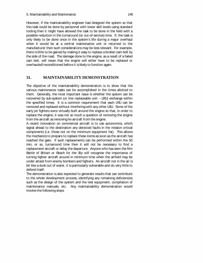
5. Maintainability and Maintenance 146
However, if the maintainability engineer had designed the system so thatthis task could be done by personnel with lower skill levels using standardtooling then it might have allowed the task to be done in the field with apossible reduction in the turnaround (or out-of-service) time. If, the task isonly likely to be done once in the system’s life during a major overhaulwhen it would be at a central maintenance unit or returned to themanufacturer then such considerations may be less relevant. For example,there is little to be gained by making it easy to replace a broken cam belt bythe side of the road. The damage done to the engine, as a result of a failedcam belt, will mean that the engine will either have to be replaced oroverhauled/reconditioned before it is likely to function again.
31. MAINTAINABILITY DEMONSTRATION
The objective of the maintainability demonstration is to show that thevarious maintenance tasks can be accomplished in the times allotted tothem. Generally, the most important issue is whether the system can berecovered by sub-system (or line replaceable unit – LRU) exchange withinthe specified times. It is a common requirement that each LRU can beremoved and replaced without interfering with any other LRU. Some of theearly jet fighters were virtually built around the engine so that, in order toreplace the engine, it was not so much a question of removing the enginefrom the aircraft as removing he aircraft from the engine.A recent innovation on commercial aircraft is to use autonomics, whichsignal ahead to the destination any detected faults in the mission criticalcomponents (i.e. those not on the minimum equipment list). This allowsthe mechanics to prepare to replace these items as soon as the aircraft hasreached the gate. If such replacements can be performed within the 50min, or so, turnaround time then it will not be necessary to find areplacement aircraft or delay the departure. Anyone who has seen the filmBattle of Britain or Reach for the Sky will recognise the importance ofturning fighter aircraft around in minimum time when the airfield may beunder attack from enemy bombers and fighters. An aircraft not in the air isbit like a duck out of water, it is particularly vulnerable and do very little todefend itself.The demonstration is also expected to generate results that can contributeto the whole development process, identifying any remaining deficienciessuch as the design of the system and the test equipment, compilation ofmaintenance manuals, etc. Any maintainability demonstration wouldinvolve the following steps:
5. Maintainability and Maintenance 147
1. Identify the operation and environmental condition in which thesystem is likely to be used.
2. Simulate the system failures and perform corrective maintenanceaction. One should also record the maintenance man-hoursrequired to complete the repair task successfully.
Further, it is an important to take care of the following issues during thedemonstration:
1. The test must be on a sample of fixed final build standard.2. The test conditions must be representative, the equipment/tools,
maintenance manuals, lighting and similar factors must be carefullyconsidered.
3. A mix of repairers representative in skills, training, and experience ofthose who would do the actual repair in service must conduct therepair.
Once we have the recorded repair time data from the above procedure,then it is easy to verify whether the maintainability target has beenachieved using the following procedure.Let t1, t2, …, tn denote the observed repair times to complete the repairtasks for a sample of n units. For n > 30, the (1 - α) 100 percent confidencelimit is given by:
nszMTTR α+ (5.8)
Where zα is the z value (standard normal statistic) that locates an area of αto its right and can be found from the normal table. For example, for a 95%confidence limit, the zα is given by 1.645. MTTR and 's' are given by:
∑==
n
iitn
MTTR1
1 , and ∑ −−
==
n
ii MTTRt
ns
1
22 )(1
1
If the target maintainability is MTTR*, then to demonstrate that the systemhas achieved this, we have to show that:
nszMTTRMTTR α+≤* (5.9)
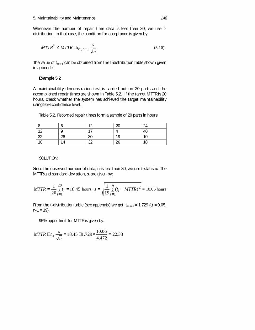
5. Maintainability and Maintenance 148
Whenever the number of repair time data is less than 30, we use t-distribution; in that case, the condition for acceptance is given by:
nstMTTRMTTR n 1,
*−+≤ α (5.10)
The value of tα,n-1 can be obtained from the t-distribution table shown givenin appendix.
Example 5.2
A maintainability demonstration test is carried out on 20 parts and theaccomplished repair times are shown in Table 5.2. If the target MTTR is 20hours, check whether the system has achieved the target maintainabilityusing 95% confidence level.
Table 5.2. Recorded repair times form a sample of 20 parts in hours
8 6 12 20 2412 9 17 4 4032 26 30 19 1010 14 32 26 18
SOLUTION:
Since the observed number of data, n is less than 30, we use t-statistic. TheMTTR and standard deviation, s, are given by:
45.18201 20
1=∑=
=iitMTTR hours, ∑ −=
=
n
ii MTTRts
1
2)(191
= 10.06 hours
From the t-distribution table (see appendix) we get, tα, n-1 = 1.729 (α = 0.05,n-1 = 19).
95% upper limit for MTTR is given by:
33.22472.406.10729.145.18 =×+=+
nstMTTR α
5. Maintainability and Maintenance 149
Which is greater than 20 hours, which is the target MTTR. Thus theachieved MTTR is significantly greater than the required MTTR and istherefore not acceptable.
32. MAINTENANCE
According to BS 4778, maintenance can be defined as:
The combination of all technical and administrative actions, includingsupervision actions, intended to retain an item in, or restore it to, a state inwhich it can perform a required function.
In other words, all actions, which keep the system running and ensure thatit is maintained to an acceptable standard in which it is able to operate atthe required levels efficiently and effectively. The objectives ofmaintenance are to:
1. Reduce the consequences of failure.2. Extend the life of the system, by keeping the system in a proper condition
for a longer time. In other words, to increase the up time of the system.3. Ensure that the system is fit and safe to use.4. Ensure that the condition of the system meets all authorised
requirements.5. Maintain the value of the system.6. Maintain reliability and achieve a high level of safety.7. Maintain the system's availability and therefore minimise production and
quality losses.8. Reduce overall maintenance costs and therefore minimise the life cycle
cost.
The purpose of maintenance is to keep systems in a state of functioning inaccordance with their design and to restore them to a similar state as andwhen required.
33. MAINTENANCE CONCEPT
The maintenance concept begins with a series of statements defining theinput criteria to which the system should be designed. These statementsrelate to the maintenance tasks that should be performed at each level of
5. Maintainability and Maintenance 150
maintenance (organisational, intermediate and depot), the test equipmentand tools that should be used in maintaining the system, the skill levels ofthe maintenance personnel that perform the identified tasks, maintenancetime constraints, and anticipated maintenance environmental requirements(Knezevic, 1997). A preliminary maintenance concept is developed duringthe conceptual design stage, is continually updated, and is a prerequisite tosystem design and development. Maintenance concept at the design phasetends to ensure that all functions of design and support are integrated witheach other. The maintenance concept evolved from the definition ofsystem operational requirements delineates [Blanchard et. al., 1995]
• The anticipated level of maintenance• Overall repair policies• Elements of maintenance resources• The organisational responsibilities for maintenance
The maintenance concept serves the following purposes:
1. It provides the basis for the establishment of maintainability andsupportability requirements in the system design.
2. It provides the basis for the establishment of requirements for totalsupport which include maintenance tasks, task frequencies and time,personnel quantities and skill levels, spare parts, facilities, and otherresources.
3. It provides a basis for detailing the maintenance plan and impacts uponthe elements of logistic support.
34. LEVELS OF MAINTENANCE
Complex systems can be considered as made up of several levels ofindenture. A combat aircraft that may be considered as the Level 0 (LoI-0),may be thought of as consisting five subsystems: airframe, armament,avionics, propulsion and general. The propulsion system then becomes aLoI-1 item that may consist of the engines, the auxiliary power unit (APU)and various accessories including control units and pumps, each of whichmay be considered as LoI-2 items. An engine is typically an assembly of anumber of modules or LoI-3 items which, in turn, may be made up of sub-assemblies and parts, LoI-4 and 5 respectively.At the same time, the military typically divides its maintenance and supportinfrastructure into 3, 4 or 5 echelons, lines or [maintenance] levels. “First

5. Maintainability and Maintenance 151
Line”, or “O-Level” is from where the systems are operated. “Second Line”or “I-Level” is typically the main operational bases from which thesquadrons are deployed. These are usually supported by a depot ormaintenance unit at “Third Line” or “D-Level”. The contractor, supplier ororiginal equipment manufacturer (OEM) often provides a shadow facility at“Fourth Line” effectively duplicating the Third Line facility’s capabilities. Maintenance levels are concerned with grouping the tasks for eachlocation where maintenance activities are performed. The criteria in whichthe maintenance tasks selected at each level are; task complexity,personnel skill-level requirements, special maintenance equipment andresources and economic measures. Within the scope of the identified levelof maintenance, the manufacturer and the user should define a basic repairpolicy that may vary from repair/replace a part (LoI-5, say) to replace theentire system. The hierarchies of achieving maintenance tasks are dividedinto three or four levels.
34.1 User level (organisational)
This type of maintenance level is related to all maintenance tasks which areperformed on the system whilst it is on deployment or at its operating site.This would include replenishment tasks, e.g. re-fuelling, re-arming,maintaining oil levels, simple condition and performance monitoringactivities, external adjustments and replacement of line replaceable units(LRU). Some minor repairs and routine servicing may also come under thiscategory.
34.2 Intermediate level
Intermediate maintenance level is related to all maintenance tasks, whichare performed at workshops (mobile, semi-mobile and/or fixed) where thesystems would normally be based. Common maintenance tasksaccomplished at this level are detailed condition and performancemonitoring activities, repair and replacement of major items in a system,major overhaul, system modification, etc. Performing maintenance tasks atthis level require higher personnel skills than those at organisational leveland additional maintenance resources. Traditionally, a removed LRUwould be recovered, generally by module (or shop-replaceable unit – SRU)exchange, at this level.
5. Maintainability and Maintenance 152
34.3 Depot level
Depot maintenance level is related to all maintenance tasks, which areaccomplished beyond the capabilities of intermediate level at remote sites.In the UK system, “Third Line” refers specifically to an operator-ownedfacility whereas in US nomenclature “D-Level” also includesmanufacturer/contractor facilities. Maintenance tasks at this level arecarried out by highly skilled specialists at a specialised repair facility or theequipment producer’s facility. Maintenance tasks at depot level includecomplete overhauling and rebuilding of the system, highly complexmaintenance actions, etc. They would also include tasks which may only beperformed rarely, particularly if they require expensive equipment or arelikely to take a long time.
34.4 Hole-in-the-Wall
With the move to ever greater efficiency and/or minimal costs, theperceived need to reduce manning levels and the desire of OEMs toincrease their revenue by entering the “after-market”, the “hole-in-the-wall” concept is gaining in popularity. This is where the only intrusivemaintenance task the operator performs is to remove the LRU (at first line).This is then passed through this mythical hole in the wall to the OEM ormaintenance contractor in exchange for a replacement (serviceable) LRU.The contractor then takes the LRU away to a convenient location where it isrecovered. Such contracts are often funded by fleet hour arrangementssuch as “power-by-the-hour”, see chapter 12.The advantage to the operators is that they can get on with what they arein business for; putting “bums on seats” or “bombs on target”. It is alsoargued, perhaps more strongly by the OEM than the operator, that havingdesigned and built the LRU, they (the OEM) are the best people to take itapart and repair it. A secondary advantage to the OEM, and again,hopefully to the operator, is that because all of the maintenance is done inone place, the people doing it should become more efficient (as they seethe same job more often) and the in-service data (time to failure, cause offailure, items repaired or replaced, etc.) should be consistent and moreaccurate.Better data should lead to improved forecasting, reduced logistic delays,more appropriate maintenance policies and, ultimately, to improveddesigns.
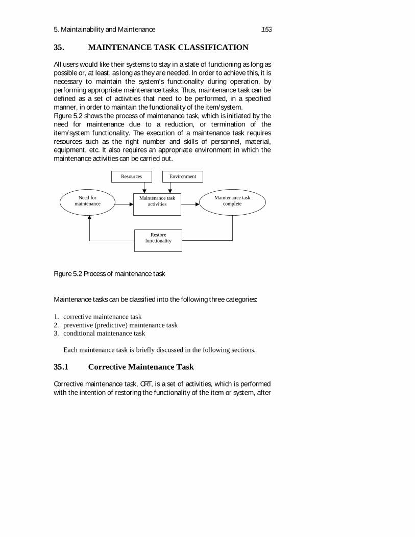
5. Maintainability and Maintenance 153
35. MAINTENANCE TASK CLASSIFICATION
All users would like their systems to stay in a state of functioning as long aspossible or, at least, as long as they are needed. In order to achieve this, it isnecessary to maintain the system’s functionality during operation, byperforming appropriate maintenance tasks. Thus, maintenance task can bedefined as a set of activities that need to be performed, in a specifiedmanner, in order to maintain the functionality of the item/system.Figure 5.2 shows the process of maintenance task, which is initiated by theneed for maintenance due to a reduction, or termination of theitem/system functionality. The execution of a maintenance task requiresresources such as the right number and skills of personnel, material,equipment, etc. It also requires an appropriate environment in which themaintenance activities can be carried out.
Figure 5.2 Process of maintenance task
Maintenance tasks can be classified into the following three categories:
1. corrective maintenance task2. preventive (predictive) maintenance task3. conditional maintenance task
Each maintenance task is briefly discussed in the following sections.
35.1 Corrective Maintenance Task
Corrective maintenance task, CRT, is a set of activities, which is performedwith the intention of restoring the functionality of the item or system, after
Maintenance taskactivities
Need formaintenance
Resources
Maintenance taskcomplete
Environment
Restorefunctionality
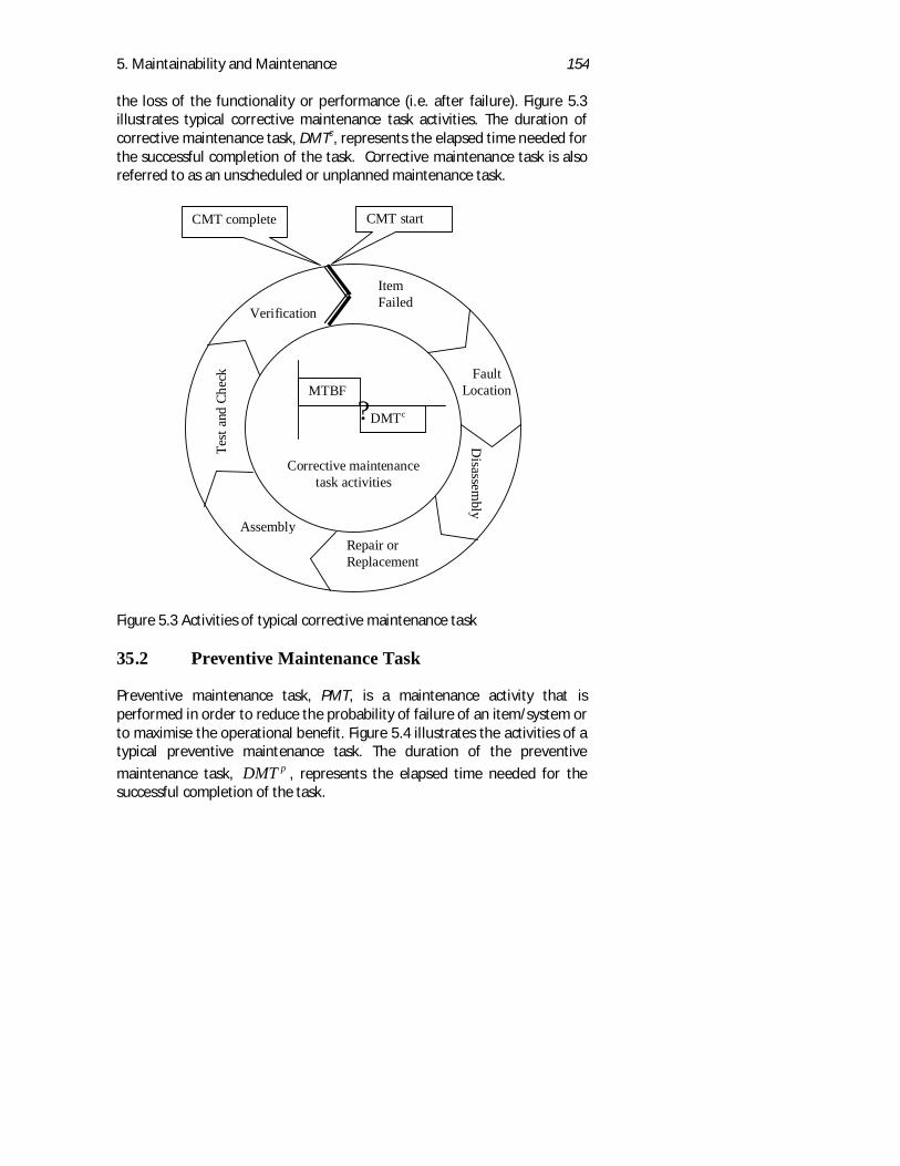
5. Maintainability and Maintenance 154
the loss of the functionality or performance (i.e. after failure). Figure 5.3illustrates typical corrective maintenance task activities. The duration ofcorrective maintenance task, DMTc, represents the elapsed time needed forthe successful completion of the task. Corrective maintenance task is alsoreferred to as an unscheduled or unplanned maintenance task.
Figure 5.3 Activities of typical corrective maintenance task
35.2 Preventive Maintenance Task
Preventive maintenance task, PMT, is a maintenance activity that isperformed in order to reduce the probability of failure of an item/system orto maximise the operational benefit. Figure 5.4 illustrates the activities of atypical preventive maintenance task. The duration of the preventive
maintenance task, DMT p , represents the elapsed time needed for thesuccessful completion of the task.
MTBF
DMTc?
ItemFailed
FaultLocation
Disassem
bly
Repair orReplacement
Assembly
Test
and
Chec
k
Verification
Corrective maintenancetask activities
CMT startCMT complete
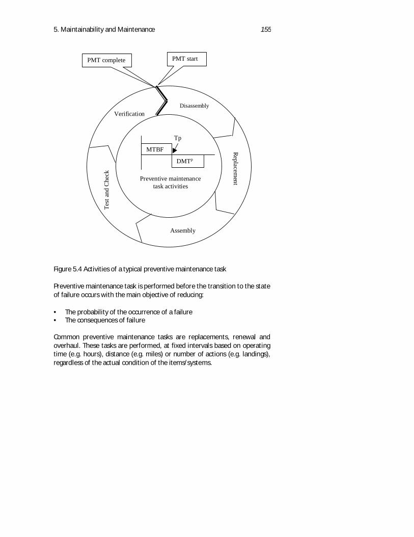
5. Maintainability and Maintenance 155
Figure 5.4 Activities of a typical preventive maintenance task
Preventive maintenance task is performed before the transition to the stateof failure occurs with the main objective of reducing:
• The probability of the occurrence of a failure• The consequences of failure
Common preventive maintenance tasks are replacements, renewal andoverhaul. These tasks are performed, at fixed intervals based on operatingtime (e.g. hours), distance (e.g. miles) or number of actions (e.g. landings),regardless of the actual condition of the items/systems.
MTBF
DMTp
Tp
Disassembly
Replacement
Assembly
Test
and
Che
ckVerification
Preventive maintenancetask activities
PMT startPMT complete
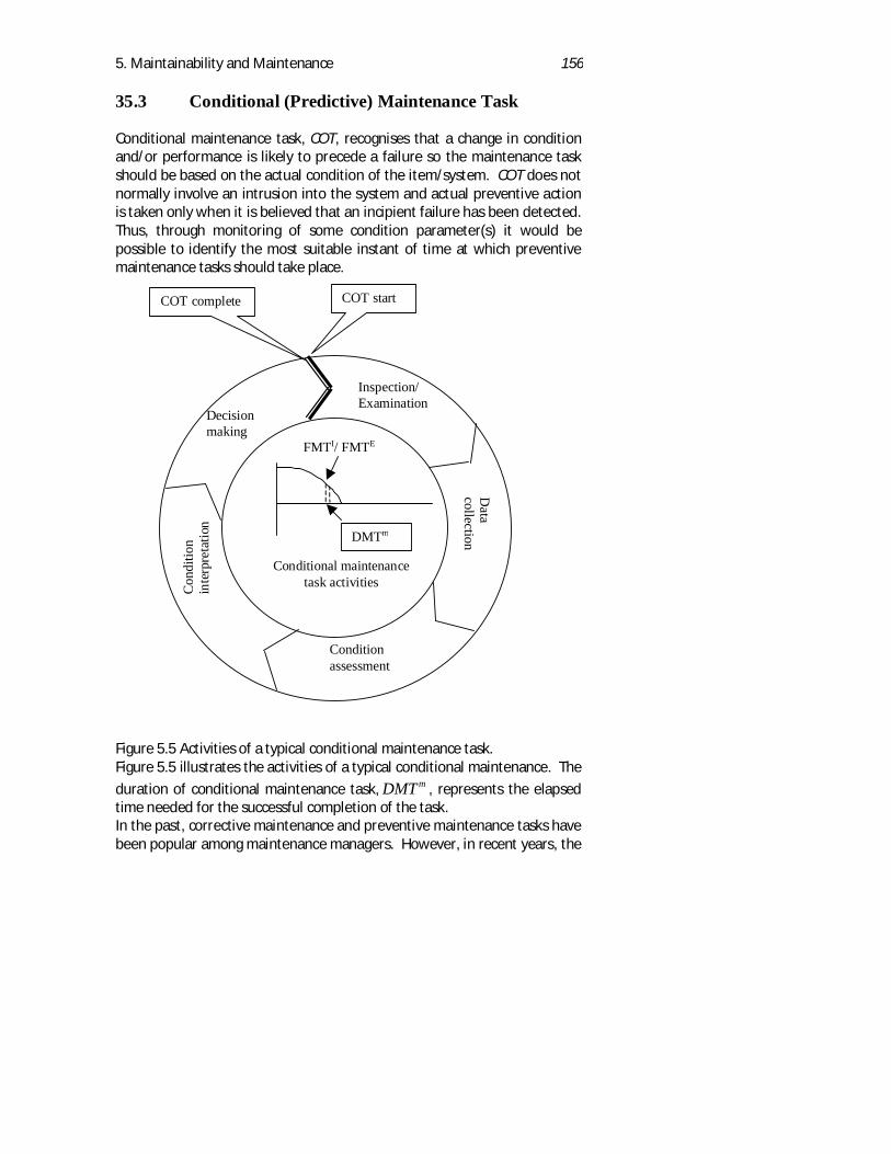
5. Maintainability and Maintenance 156
35.3 Conditional (Predictive) Maintenance Task
Conditional maintenance task, COT, recognises that a change in conditionand/or performance is likely to precede a failure so the maintenance taskshould be based on the actual condition of the item/system. COT does notnormally involve an intrusion into the system and actual preventive actionis taken only when it is believed that an incipient failure has been detected.Thus, through monitoring of some condition parameter(s) it would bepossible to identify the most suitable instant of time at which preventivemaintenance tasks should take place.
Figure 5.5 Activities of a typical conditional maintenance task.Figure 5.5 illustrates the activities of a typical conditional maintenance. The
duration of conditional maintenance task, DMT m , represents the elapsedtime needed for the successful completion of the task.In the past, corrective maintenance and preventive maintenance tasks havebeen popular among maintenance managers. However, in recent years, the
DMTm
FMTI/ FMTE
Inspection/Examination
Data
collection
Conditionassessment
Con
ditio
nin
terp
reta
tion
Decisionmaking
Conditional maintenancetask activities
COT startCOT complete
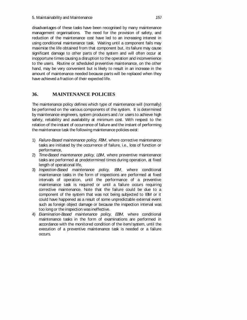
5. Maintainability and Maintenance 157
disadvantages of these tasks have been recognised by many maintenancemanagement organisations. The need for the provision of safety, andreduction of the maintenance cost have led to an increasing interest inusing conditional maintenance task. Waiting until a component fails maymaximise the life obtained from that component but, its failure may causesignificant damage to other parts of the system and will often occur atinopportune times causing a disruption to the operation and inconvenienceto the users. Routine or scheduled preventive maintenance, on the otherhand, may be very convenient but is likely to result in an increase in theamount of maintenance needed because parts will be replaced when theyhave achieved a fraction of their expected life.
36. MAINTENANCE POLICIES
The maintenance policy defines which type of maintenance will (normally)be performed on the various components of the system. It is determinedby maintenance engineers, system producers and /or users to achieve highsafety, reliability and availability at minimum cost. With respect to therelation of the instant of occurrence of failure and the instant of performingthe maintenance task the following maintenance policies exist:
1) Failure-Based maintenance policy, FBM, where corrective maintenancetasks are initiated by the occurrence of failure, i.e., loss of function orperformance,
2) Time-Based maintenance policy, LBM, where preventive maintenancetasks are performed at predetermined times during operation, at fixedlength of operational life,
3) Inspection-Based maintenance policy, IBM, where conditionalmaintenance tasks in the form of inspections are performed at fixedintervals of operation, until the performance of a preventivemaintenance task is required or until a failure occurs requiringcorrective maintenance. Note that the failure could be due to acomponent of the system that was not being subjected to IBM or itcould have happened as a result of some unpredictable external eventsuch as foreign object damage or because the inspection interval wastoo long or the inspection was ineffective.
4) Examination-Based maintenance policy, EBM, where conditionalmaintenance tasks in the form of examinations are performed inaccordance with the monitored condition of the item/system, until theexecution of a preventive maintenance task is needed or a failureoccurs.
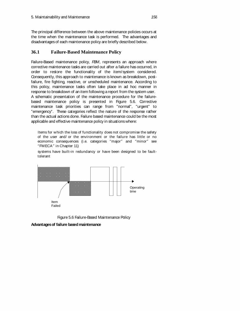
5. Maintainability and Maintenance 158
The principal difference between the above maintenance policies occurs atthe time when the maintenance task is performed. The advantages anddisadvantages of each maintenance policy are briefly described below.
36.1 Failure-Based Maintenance Policy
Failure-Based maintenance policy, FBM, represents an approach wherecorrective maintenance tasks are carried out after a failure has occurred, inorder to restore the functionality of the item/system considered.Consequently, this approach to maintenance is known as breakdown, post-failure, fire fighting, reactive, or unscheduled maintenance. According tothis policy, maintenance tasks often take place in ad hoc manner inresponse to breakdown of an item following a report from the system user.A schematic presentation of the maintenance procedure for the failure-based maintenance policy is presented in Figure 5.6. Correctivemaintenance task priorities can range from "normal", "urgent" to"emergency". These categories reflect the nature of the response ratherthan the actual actions done. Failure based maintenance could be the mostapplicable and effective maintenance policy in situations where:
Items for which the loss of functionality does not compromise the safetyof the user and/or the environment or the failure has little or noeconomic consequences (i.e. categories major and minor see
FMECA in Chapter 11)systems have built-in redundancy or have been designed to be fault-tolerant
Figure 5.6 Failure-Based Maintenance Policy
Advantages of failure based maintenance
ItemFailed
Operatingtime
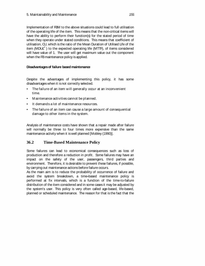
5. Maintainability and Maintenance 159
Implementation of FBM to the above situations could lead to full utilisationof the operating life of the item. This means that the non-critical items willhave the ability to perform their function(s) for the stated period of timewhen they operate under stated conditions. This means that coefficient ofutilisation, CU, which is the ratio of the Mean Duration of Utilised Life of theitem (MDULF ) to the expected operating life (MTTF), of items consideredwill have value of 1. The user will get maximum value out the componentwhen the FB maintenance policy is applied.
Disadvantages of failure based maintenance
Despite the advantages of implementing this policy, it has somedisadvantages when it is not correctly selected.
• The failure of an item will generally occur at an inconvenienttime.
• Maintenance activities cannot be planned.• It demands a lot of maintenance resources.• The failure of an item can cause a large amount of consequential
damage to other items in the system.
Analysis of maintenance costs have shown that a repair made after failurewill normally be three to four times more expensive than the samemaintenance activity when it is well planned [Mobley (1990)].
36.2 Time-Based Maintenance Policy
Some failures can lead to economical consequences such as loss ofproduction and therefore a reduction in profit. Some failures may have animpact on the safety of the user, passengers, third parties andenvironment. Therefore, it is desirable to prevent these failures, if possible,by carrying out maintenance actions before failure occurs.As the main aim is to reduce the probability of occurrence of failure andavoid the system breakdown, a time-based maintenance policy isperformed at fix intervals, which is a function of the time-to-failuredistribution of the item considered and in some cases it may be adjusted bythe system's user. This policy is very often called age-based, life-based,planned or scheduled maintenance. The reason for that is the fact that the
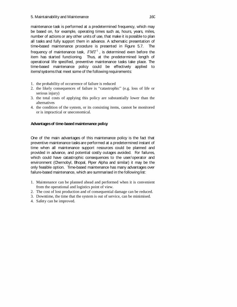
5. Maintainability and Maintenance 160
maintenance task is performed at a predetermined frequency, which maybe based on, for example, operating times such as, hours, years, miles,number of actions or any other units of use, that make it is possible to planall tasks and fully support them in advance. A schematic presentation oftime-based maintenance procedure is presented in Figure 5.7. The
frequency of maintenance task, FMT L , is determined even before theitem has started functioning. Thus, at the predetermined length ofoperational life specified, preventive maintenance tasks take place. Thetime-based maintenance policy could be effectively applied toitems/systems that meet some of the following requirements:
1. the probability of occurrence of failure is reduced2. the likely consequences of failure is catastrophic (e.g. loss of life or
serious injury)3. the total costs of applying this policy are substantially lower than the
alternatives4. the condition of the system, or its consisting items, cannot be monitored
or is impractical or uneconomical.
Advantages of time-based maintenance policy
One of the main advantages of this maintenance policy is the fact thatpreventive maintenance tasks are performed at a predetermined instant oftime when all maintenance support resources could be planned andprovided in advance, and potential costly outages avoided. For failures,which could have catastrophic consequences to the user/operator andenvironment (Chernobyl, Bhopal, Piper Alpha and similar) it may be theonly feasible option. Time-based maintenance has many advantages overfailure-based maintenance, which are summarised in the following list:
1. Maintenance can be planned ahead and performed when it is convenientfrom the operational and logistics point of view.
2. The cost of lost production and of consequential damage can be reduced.3. Downtime, the time that the system is out of service, can be minimised.4. Safety can be improved.
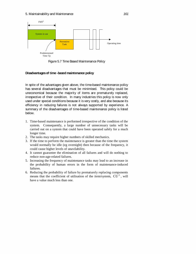
5. Maintainability and Maintenance 161
Figure 5.7 Time Based Maintenance Policy
Disadvantages of time -based maintenance policy
In spite of the advantages given above, the time-based maintenance policyhas several disadvantages that must be minimised. This policy could beuneconomical because the majority of items are prematurely replaced,irrespective of their condition. In many industries this policy is now onlyused under special conditions because it is very costly, and also because itsefficiency in reducing failures is not always supported by experience. Asummary of the disadvantages of time-based maintenance policy is listedbelow.
1. Time-based maintenance is performed irrespective of the condition of thesystem. Consequently, a large number of unnecessary tasks will becarried out on a system that could have been operated safely for a muchlonger time.
2. The tasks may require higher numbers of skilled mechanics.3. If the time to perform the maintenance is greater than the time the system
would normally be idle (eg overnight) then because of the frequency, itcould cause higher levels of unavilability.
4. It cannot guarantee the elimination of all failures and will do nothing toreduce non-age-related failures.
5. Increasing the frequency of maintenance tasks may lead to an increase inthe probability of human errors in the form of maintenance-inducedfailures.
6. Reducing the probability of failure by prematurely replacing componentsmeans that the coefficient of utilisation of the item/system, CU L , willhave a value much less than one.
PreventiveTask
System in use
PredeterminedTime Tp
Operating time
FMTL
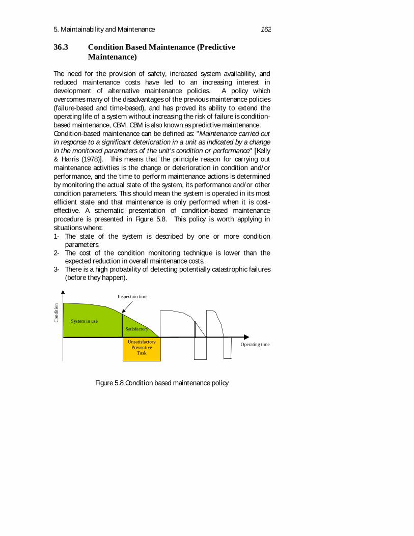
5. Maintainability and Maintenance 162
36.3 Condition Based Maintenance (PredictiveMaintenance)
The need for the provision of safety, increased system availability, andreduced maintenance costs have led to an increasing interest indevelopment of alternative maintenance policies. A policy whichovercomes many of the disadvantages of the previous maintenance policies(failure-based and time-based), and has proved its ability to extend theoperating life of a system without increasing the risk of failure is condition-based maintenance, CBM. CBM is also known as predictive maintenance.Condition-based maintenance can be defined as: "Maintenance carried outin response to a significant deterioration in a unit as indicated by a changein the monitored parameters of the unit's condition or performance" [Kelly& Harris (1978)]. This means that the principle reason for carrying outmaintenance activities is the change or deterioration in condition and/orperformance, and the time to perform maintenance actions is determinedby monitoring the actual state of the system, its performance and/or othercondition parameters. This should mean the system is operated in its mostefficient state and that maintenance is only performed when it is cost-effective. A schematic presentation of condition-based maintenanceprocedure is presented in Figure 5.8. This policy is worth applying insituations where:1- The state of the system is described by one or more condition
parameters.2- The cost of the condition monitoring technique is lower than the
expected reduction in overall maintenance costs.3- There is a high probability of detecting potentially catastrophic failures
(before they happen).
Figure 5.8 Condition based maintenance policy
UnsatisfactoryPreventive
Task
System in use
Inspection time
Operating time
Satisfactory
Cond
ition
System in use
5. Maintainability and Maintenance 163
The condition-based maintenance is a condition or performance-drivenpreventive maintenance. This means that the timing of the maintenancetask is not simply a function of the mean-time-to-failure. The principle ofcondition-based maintenance therefore is based on the way of monitoringthe condition parameters of a system giving three different types ofcondition monitoring:
1- Inspection
Inspection is generally performed at regular intervals using any of a numberof non-destructive test (NDT) procedures which are designed to determinewhether the condition of the (inspected) item is satisfactory orunsatisfactory and hence whether further action is required.
2- Examination
This is a condition-monitoring task, which presents a numerical descriptionof the condition of the item at that moment through relevant conditionpredictors. The results directly affect the scheduling of the nextexamination. This is possible because of the unique properties andcharacteristics of the relevant condition predictor.
3 - Performance Trend Monitoring
For propulsion or energy producing systems, in particular, theperformance may be expressed as a ratio of the output to input, e.g. milesper gallon, kilometres per litre, thrust per kilogram or (mega)watts per
tonne. As the system deteriorates, usually through wear but also throughdamage, these ratios may show signs of decreasing. For systems operating
in relatively constant conditions (e.g. constant ambient temperature,pressure and output), consistent changes in the specific fuel consumption(SFC) will almost certainly be indicative of a deterioration in the systemwhich will need some form of maintenance to restore it to an acceptable
level. For systems that are operated in an inconsistent manor for which theenvironmental conditions may be in a constant state of change, the SFC may
be subject to considerable noise and hence any deterioration will only beapparent by using sophisticated trending algorithms, such as Kalman
Filtering.
5. Maintainability and Maintenance 164
36.3.1Setting up condition-based maintenance policy
In order to implement CBM policy, it is necessary to use the followingmanagement steps that are shown in Figure 5.9
Identification and selection of maintenance significant items
The first requirement of implementing CBM is to decide which items of thesystem should be monitored, since it is likely to be both uneconomical andimpractical to monitor them all. Therefore, the first step of the condition-based maintenance decision process is a comprehensive review of all itemsin a system, in order to identify the maintenance significant items, MSIs.These are items whose failures could be safety-critical, environmentallydamaging or revenue sensitive. Thus, each item within the system shouldbe analysed from the point of view of failure, especially the consequencesof failure. The most frequently used engineering tools for performing thistask is a Failure Mode Effect and Criticality Analysis, FMECA and ReliabilityCentred Maintenance, RCM (see also Chapters 6 and 11). Care should betaken to ensure that all of the maintenance significant items are identifiedand listed.
Identification and selection of condition parameters
Once the maintenance significant items are identified it is necessary todetermine all monitorable parameters which describe their condition orperformance. The condition parameter can be defined as a measurablevariable able to display directly or reflect indirectly information about thecondition of an item at any instance of operating time. Ideally, maintenanceengineers would like to find many condition/parameters which can bemonitored and which accurately reflects the condition /performance of thesystem. In practice there are two distinguishable types of conditionparameters which are able to achieve this (Knezevic et al, 1995):
A. Relevant Condition Indicator, RCI
The Relevant Condition Indictor, RCI, is a parameter that describes thecondition of an item during its operating time and it indicates the condition
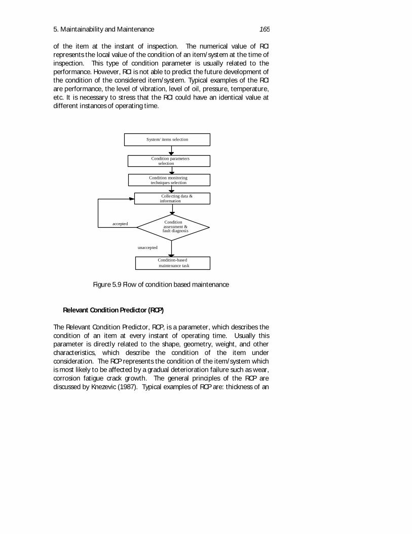
5. Maintainability and Maintenance 165
of the item at the instant of inspection. The numerical value of RCIrepresents the local value of the condition of an item/system at the time ofinspection. This type of condition parameter is usually related to theperformance. However, RCI is not able to predict the future development ofthe condition of the considered item/system. Typical examples of the RCIare performance, the level of vibration, level of oil, pressure, temperature,etc. It is necessary to stress that the RCI could have an identical value atdifferent instances of operating time.
Figure 5.9 Flow of condition based maintenance
Relevant Condition Predictor (RCP)
The Relevant Condition Predictor, RCP, is a parameter, which describes thecondition of an item at every instant of operating time. Usually thisparameter is directly related to the shape, geometry, weight, and othercharacteristics, which describe the condition of the item underconsideration. The RCP represents the condition of the item/system whichis most likely to be affected by a gradual deterioration failure such as wear,corrosion fatigue crack growth. The general principles of the RCP arediscussed by Knezevic (1987). Typical examples of RCP are: thickness of an
System/ items selection
Condition parametersselection
Condition monitoringtechniques selection
Collecting data &information
fault diagnosis
Conditionassessment &
Condition-basedmaintenance task
accepted
unaccepted
5. Maintainability and Maintenance 166
item, crack length, depth of tyre treads, etc. The RCP cannot have identicalvalues at two or more instance of time. The numerical value of the relevantcondition predictor at any instant of operating time quantifies thecumulative value of the condition of an item/system at the time ofexamination.
Selection of condition monitoring technique
Having identified the maintenance significant item and the associatedcondition parameter(s), the next step is to select the suitable monitoringtechnique, which will be used to inspect and examine each conditionparameter.The condition monitoring technique is a device used to inspect or examinean item in order to provide data and information about its condition at anyinstance of operating time. Numerous condition monitoring techniques, forinstance, NDT techniques, performance, vibration, etc are available for useby maintenance engineers in order to determine measurable value ofcondition parameter. It is important to understand the behaviour of thefailure that the item exhibits so that the most effective monitoringtechniques can be chosen.The decision as to which condition-monitoring techniques are selecteddepends greatly on the type of system, the type of condition parameterand, in the end, on cost and safety. Once the decision is made as to whichtechniques are to be used, it is possible to define the equipment orinstrument that will be needed to carry out condition monitoring.
Collecting data and information
The philosophy of condition monitoring is to assess the condition of anitem/system by the use of techniques which can range from human sensingto sophisticated instrumentation, in order to determine the need forperforming preventive maintenance tasks. With the increased interest incondition monitoring in recent years there have been a number ofdevelopments in the techniques that are used to collect data and provideinformation, which helps maintenance engineers assessing the condition ofan item or a system. These developments have made it possible to obtainmore reliable information on the condition of the system. In manyinstances such information is used to insure that the status of the systemwill continue to be in a functioning state without significant risk of
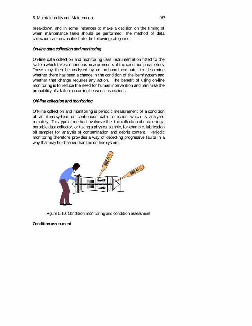
5. Maintainability and Maintenance 167
breakdown, and in some instances to make a decision on the timing ofwhen maintenance tasks should be performed. The method of datacollection can be classified into the following categories:
On-line data collection and monitoring
On-line data collection and monitoring uses instrumentation fitted to thesystem which takes continuous measurements of the condition parameters.These may then be analysed by an on-board computer to determinewhether there has been a change in the condition of the item/system andwhether that change requires any action. The benefit of using on-linemonitoring is to reduce the need for human intervention and minimise theprobability of a failure occurring between inspections.
Off-line collection and monitoring
Off-line collection and monitoring is periodic measurement of a conditionof an item/system or continuous data collection which is analysedremotely. This type of method involves either the collection of data using aportable data collector, or taking a physical sample, for example, lubricationoil samples for analysis of contamination and debris content. Periodicmonitoring therefore provides a way of detecting progressive faults in away that may be cheaper than the on-line system.
Figure 5.10. Condition monitoring and condition assessment
Condition assessment
5. Maintainability and Maintenance 168
The assessment of the condition of an item/system (Figure 5.10) can rangefrom human experience to sophisticated instrumentation. The last fewdecades have seen a number of developments in the methods which areused to help the maintenance engineers assess and diagnose the conditionof an item/system and provide them with information on which to basetheir decision. Once condition monitoring sensors have been installed anddata are being collected, it is necessary to have reliable methods ofinterpreting the data to identify whether the considered item is undergoinga transition from the normal to abnormal condition and in many cases toidentify the causes of the changes.Effective condition-based maintenance requires a large number ofmeasurements taken continuously or at intervals that assure recognition ofchange in the condition of the item/system in sufficient time to avoid theneed for any corrective action. The volume of data necessary to accuratelydetermine the condition of the item/system can require an excessiveamount of time to process and analyse. Consequently, the demand tomanipulate and process large amounts of data very quickly has lead to thedevelopment of tools such as Artificial Intelligence, AI, to assist engineers togain maximum value from the data.In recent years, Artificial Intelligence techniques such as Expert System,Neural Networks and Fuzzy Logic have been applied to the discipline ofmonitoring and diagnostic systems [Mann et al (1995)]. These techniquesextend the power of the computer beyond the usual mathematical andstatistical functions by using dialogue and logic to determine variouspossible courses of action or outcome. By processing information muchfaster (than humans) the time to assess the condition and diagnose thecauses of failures can be reduced. It can analyse situations objectively andwill not forget any relevant facts (given that it has been supplied them),therefore the probability of making a wrong assessment or diagnosis maybe reduced. Furthermore, it can detect incipient failures through its on-linemonitoring of the condition parameters of the system [Lavalle et al (1993)].
Implementation of condition based maintenance
Having identified and listed all the condition parameters of themaintenance significant items, the aim of this step is to implementcondition based maintenance. According to the classifications of conditionparameter, condition based maintenance could be divided in two policies:
Inspection Based Maintenance Policy
5. Maintainability and Maintenance 169
The suitable maintenance policy for items for which their conditions aredescribed by the relevant condition indicator, RCI is inspection-basedmaintenance. The algorithm, which presents the maintenance procedure inthis case, is shown in Figure 5.11
Inspection is carried at fixed intervals to determine whether thecondition of the item, is satisfactory or unsatisfactory according to the RCI.Before the item/system is introduced into service the most suitable
frequency of the inspection, FMT I , and critical value of relevant conditionindicator crRCI has to be determined. Once the critical level is reached,
RCI FMT RCIIcr( ) > , the prescribed preventive maintenance tasks take
place. If the item fails between inspections, corrective maintenance takesplace.
Advantages of inspection based maintenance
CBM has the potential to produce large savings simply by allowing items inthe system to be run to the end of their useful life. This reduces theequipment down time and minimises both scheduled and unscheduledbreakdown situations. By eliminating all unscheduled interruptions tooperation and production and only carrying out required maintenance in acarefully controlled manner, it is possible to reduce the maintenance cost,to improve safety, improve the efficiency of the operation and increase thesystem’s availability.
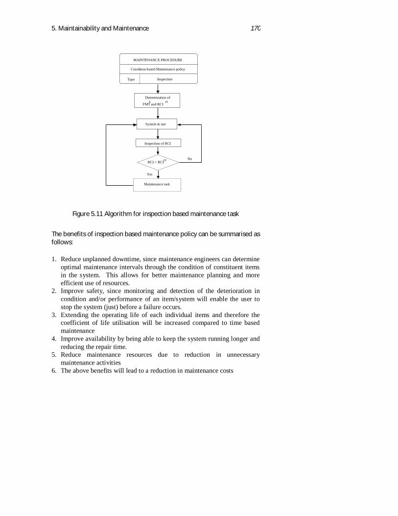
5. Maintainability and Maintenance 170
Figure 5.11 Algorithm for inspection based maintenance task
The benefits of inspection based maintenance policy can be summarised asfollows:
1. Reduce unplanned downtime, since maintenance engineers can determineoptimal maintenance intervals through the condition of constituent itemsin the system. This allows for better maintenance planning and moreefficient use of resources.
2. Improve safety, since monitoring and detection of the deterioration incondition and/or performance of an item/system will enable the user tostop the system (just) before a failure occurs.
3. Extending the operating life of each individual items and therefore thecoefficient of life utilisation will be increased compared to time basedmaintenance
4. Improve availability by being able to keep the system running longer andreducing the repair time.
5. Reduce maintenance resources due to reduction in unnecessarymaintenance activities
6. The above benefits will lead to a reduction in maintenance costs
MAINTENANCE PROCEDURE
Condition-based Maintenance policy
System in use
Maintenance task
Type Inspection
Inspection of RCI
Yes
No
Determination of
RCI > RCIcr
crFMT and RCI
I
5. Maintainability and Maintenance 171
Examination Based Maintenance Policy
The decision for performing the condition-based maintenance tasks isbased on the information related to the condition of an item/systemestablished through condition checks during its operational life. Thisindicates that inspection-based maintenance strategy has achieved thedemand for increasing the level of utilisation of an item/system. However,the system availability may not increase, due to an increased number ofinterruptions of the operation caused by increasing the number ofinspections. Therefore, as an alternative, examination based maintenanceapproach is proposed by Knezevic (1987b) for the determination ofmaintenance tasks based on relevant condition predictors.Examination based maintenance provides additional information about thechange in condition of the items considered during its operational life.Consequently, examination based maintenance was developed for thecontrol of maintenance procedures [El-Haram 1995]. With moreinformation about the process of change in condition, a higher level ofutilisation of the items can be achieved whilst maintaining a low probabilityof failure during the operation.It is a dynamic process because the time of the next examination is fullydetermined by the real condition of the system at the time of examination.Dynamic control of maintenance tasks allows each individual item toperform the requested function with the required probability of failure, asin the case of time-based preventive maintenance but with fuller utilisationof operating life, hence with a reduction of total cost of operation andproduction.The critical level of the relevant condition predictor RCPcr , sets the limitabove which appropriate maintenance tasks should be performed. Theinterval between the limit ( limRCP ) and critical values depends on theability of the operator to measure the condition of the item through theRCP . The item under consideration could be in one of the following threestates, according to the numerical value of the RCP ,:
1. RCP RCP l RCPinitial cr< <( ) : continue with examinations;
2. RCP RCP l RCPcr < <( ) lim : preventive maintenance task required;
3. RCP RCP llim ( )< : corrective maintenance task, because the failurehas already occurred.
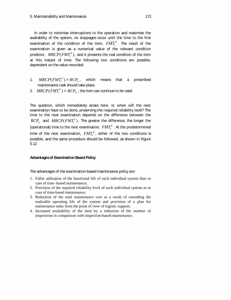
5. Maintainability and Maintenance 172
In order to minimise interruptions to the operation and maximise theavailability of the system, no stoppages occur until the time to the first
examination of the condition of the item, FMT E1 . The result of the
examination is given as a numerical value of the relevant condition
predictor, MRCP FMT E( )1 , and it presents the real condition of the itemat this instant of time. The following two conditions are possible,dependent on the value recorded:
1. MRCP FMT RCPEcr( )1 > , which means that a prescribed
maintenance task should take place.
2. MRCP FMT RCPEcr( )1 < , the item can continue to be used.
The question, which immediately arises here, is: when will the nextexamination have to be done, preserving the required reliability level? Thetime to the next examination depends on the difference between the
RCPcr and MRCP FMT E( )1 . The greater the difference, the longer the
(operational) time to the next examination, FMT E2 . At the predetermined
time of the next examination, FMTnE , either of the two conditions is
possible, and the same procedure should be followed, as shown in Figure5.12
Advantages of Examination Based Policy
The advantages of the examination-based maintenance policy are:
1. Fuller utilisation of the functional life of each individual system than incase of time -based maintenance;
2. Provision of the required reliability level of each individual system as incase of time-based maintenance;
3. Reduction of the total maintenance cost as a result of extending therealisable operating life of the system and provision of a plan formaintenance tasks from the point of view of logistic support;
4. Increased availability of the item by a reduction of the number ofinspections in comparison with inspection-based maintenance.
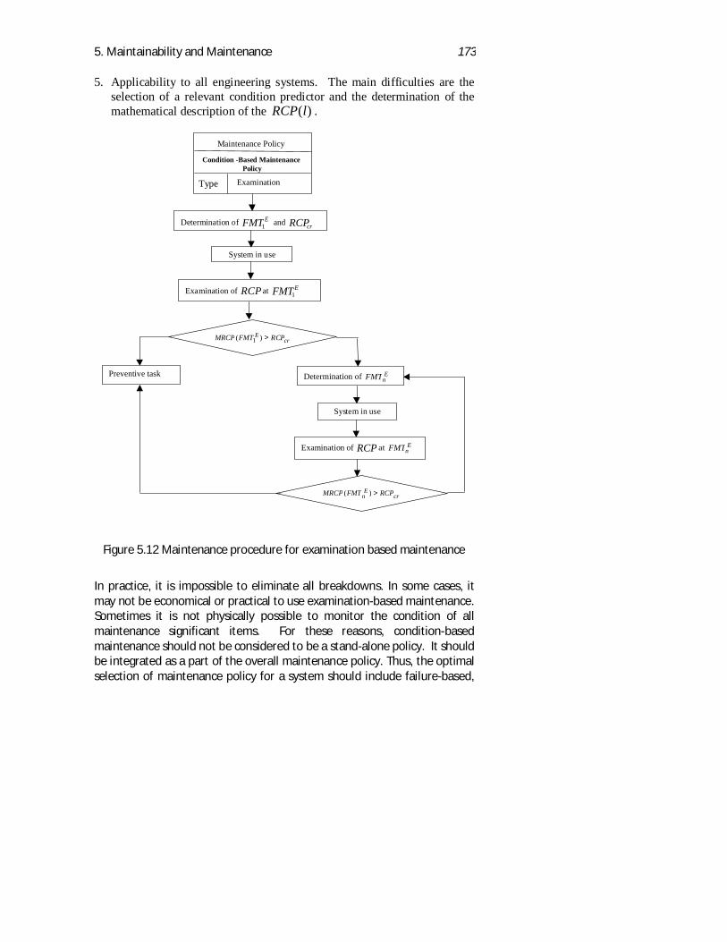
5. Maintainability and Maintenance 173
5. Applicability to all engineering systems. The main difficulties are theselection of a relevant condition predictor and the determination of themathematical description of the RCP l( ) .
Figure 5.12 Maintenance procedure for examination based maintenance
In practice, it is impossible to eliminate all breakdowns. In some cases, itmay not be economical or practical to use examination-based maintenance.Sometimes it is not physically possible to monitor the condition of allmaintenance significant items. For these reasons, condition-basedmaintenance should not be considered to be a stand-alone policy. It shouldbe integrated as a part of the overall maintenance policy. Thus, the optimalselection of maintenance policy for a system should include failure-based,
crE
n RCPFMTMRCP >)(
Maintenance Policy
Condition -Based MaintenancePolicy
Type Examination
Determination of EFMT1 and crRCP
System in use
Examination of RCP at EFMT1
crE RCPFMTMRCP >)( 1
Determination of EnFMTPreventive task
System in use
Examination of RCP at EnFMT
5. Maintainability and Maintenance 174
time-based, inspection -based and examination-based maintenancestrategies. The reasons for this are summarised below:1. Not all items in the system are significant; the suitable maintenance
policy is therefore, failure-based maintenance.2. It may not be possible or practical to monitor the condition / performance
of the significant items, so the suitable maintenance policy is therefore,time-based maintenance.
3. If the condition parameters of a significant item cannot be described by arelevant condition predictor, then the suitable maintenance policy isinspection-based maintenance
4. For significant items with relevant condition predictors, the most suitablepolicy is examination-based maintenance.
A maintenance management approach such as reliability centredmaintenance could be used to select the most applicable and effectivemaintenance task for each item in the system
37. MAINTENANCE RESOURCES
It is important to stress that the number of activities, their sequence andthe type and quantity of resource required mainly depends on the decisionstaken during the design phase of the item/system. The time required toperform a maintenance task will also depend on decisions made during thisphase, such as the complexity, testability, accessibility and any specialfacilities, equipment, tools or resources needed.Resources required primarily to facilitate the maintenance process will becalled Maintenance Resources, MR.. The resources needed for thesuccessful completion of every maintenance task, could be grouped intothe following categories (Knezevic 1997):
1. Maintenance Supply Support, MSS: is generic name which includes allspares, repair items, consumables, special supplies, and relatedinventories needed to support the maintenance process
2. Maintenance Test and Support Equipment, MTE: includes all tools,special condition monitoring equipment, diagnostic and check-outequipment, metrology and calibration equipment, maintenance stands andservicing and handling equipment required to support maintenance tasksassociated with the item/system. Typically, MTE can be divided into twogroups: special to type equipment (STTE) and general (to type)equipment (GTTE).
3. Maintenance Personnel, MP: required for the installation, check-out,handling, and sustaining maintenance of the item/system and its
5. Maintainability and Maintenance 175
associated test and support equipment are included in this category.Formal training for maintenance personnel required for each maintenancetask should be considered
4. Maintenance Facilities, MFC: refers to all special facilities needed forcompletion of maintenance tasks. Physical plant, real estate, portablebuildings, inspection pits, dry dock, housing, maintenance shops,calibration laboratories, and special repair and overhaul facilities must beconsidered related to each maintenance task
5. Maintenance Technical Data, MTD: necessary for check-out procedures,maintenance instructions, inspection and calibration procedures, overhaulprocedures, modification instructions, facilities information, drawingsand specifications that are necessary in the performance of systemmaintenance functions. Such data not only cover the system but test andsupport equipment, transportation and handling equipment, trainingequipment and facilities
6. Maintenance Computer Resources, MCR: refers to all computerequipment and accessories, software, program tapes/disks, data bases andso on, necessary in the performance of maintenance functions. Thisincludes both condition monitoring and diagnostics.
On the other hand, it is important to remember that each task is performedin a specific work environment that could make a significant impact on thesafety, accuracy and ease of task completion. The main environmentalfactors could be grouped as follows:
• space impediment (which reflects the obstructions imposed onmaintenance personnel during the task execution which requires themto operate in awkward positions)
• Climatic conditions such as rain/snow, solar radiation, humidity,temperature, and similar situations, which could make significantimpact on the safety, accuracy and ease of task completion.
• Platform on which maintenance task is performed (on operational site,on board a ship/submarine, space vehicle, workshops, and similar).
38. MAINTENANCE INDUCED FAILURES
Whenever the cause of failure is related to the maintenance performed onthe system, we call it maintenance-induced failure MIF. The root cause ofMIF is poor workmanship, which might lead to poor spares or materialselection, improper use of test equipment, training, working environment
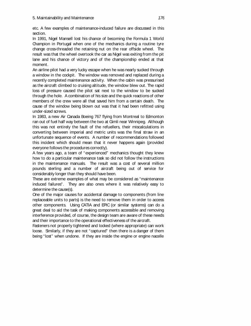
5. Maintainability and Maintenance 176
etc. A few examples of maintenance-induced failure are discussed in thissection.In 1991, Nigel Mansell lost his chance of becoming the Formula 1 WorldChampion in Portugal when one of the mechanics during a routine tyrechange cross-threaded the retaining nut on the rear offside wheel. Theresult was that the wheel overtook the car as Nigel was exiting from the pitlane and his chance of victory and of the championship ended at thatmoment.An airline pilot had a very lucky escape when he was nearly sucked througha window in the cockpit. The window was removed and replaced during arecently completed maintenance activity. When the cabin was pressurisedas the aircraft climbed to cruising altitude, the window blew out. The rapidloss of pressure caused the pilot sat next to the window to be suckedthrough the hole. A combination of his size and the quick reactions of othermembers of the crew were all that saved him from a certain death. Thecause of the window being blown out was that it had been refitted usingunder-sized screws.In 1983, a new Air Canada Boeing 767 flying from Montreal to Edmontonran out of fuel half way between the two at Gimli near Winnipeg. Althoughthis was not entirely the fault of the refuellers, their miscalculations inconverting between imperial and metric units was the final straw in anunfortunate sequence of events. A number of recommendations followedthis incident which should mean that it never happens again (providedeveryone follows the procedures correctly).A few years ago, a team of “experienced” mechanics thought they knewhow to do a particular maintenance task so did not follow the instructionsin the maintenance manuals. The result was a cost of several millionpounds sterling and a number of aircraft being out of service forconsiderably longer than they should have been.These are extreme examples of what may be considered as “maintenanceinduced failures”. They are also ones where it was relatively easy todetermine the cause(s).One of the major causes for accidental damage to components (from linereplaceable units to parts) is the need to remove them in order to accessother components. Using CATIA and EPIC (or similar systems) can do agreat deal to aid the task of making components accessible and removinginterference provided, of course, the design team are aware of these needsand their importance to the operational effectiveness of the aircraft.Fasteners not properly tightened and locked (where appropriate) can workloose. Similarly, if they are not “captured” then there is a danger of thembeing “lost” when undone. If they are inside the engine or engine nacelle
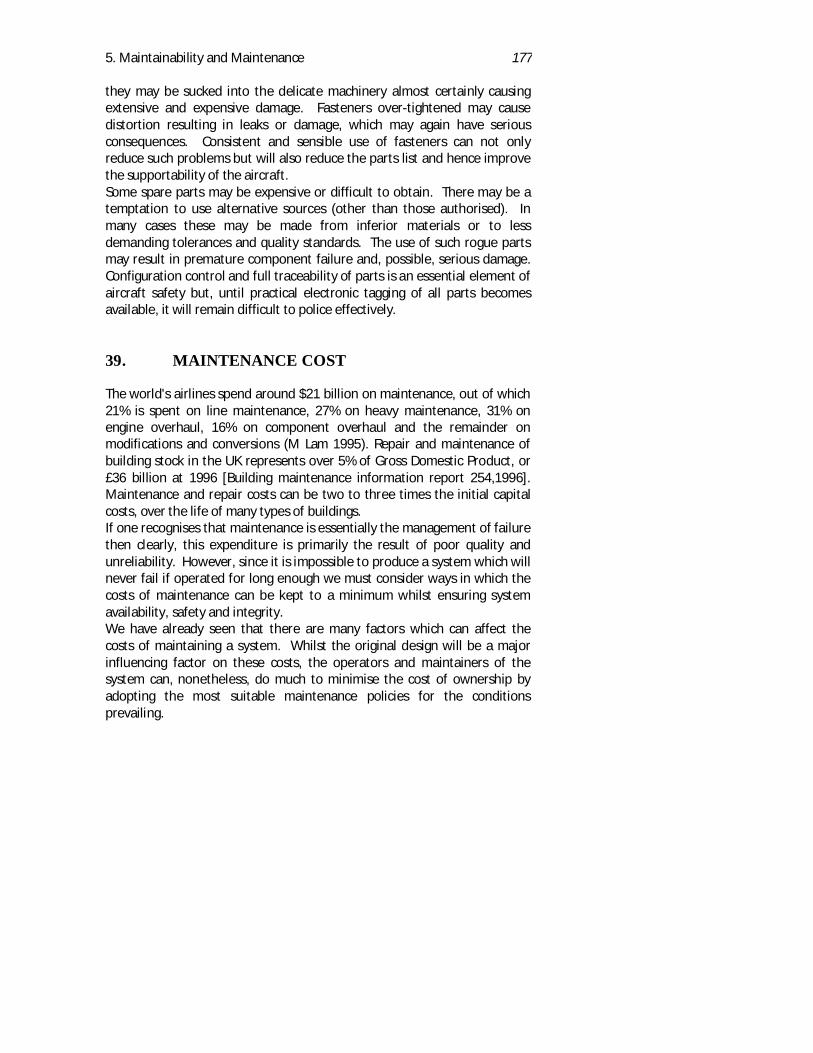
5. Maintainability and Maintenance 177
they may be sucked into the delicate machinery almost certainly causingextensive and expensive damage. Fasteners over-tightened may causedistortion resulting in leaks or damage, which may again have seriousconsequences. Consistent and sensible use of fasteners can not onlyreduce such problems but will also reduce the parts list and hence improvethe supportability of the aircraft.Some spare parts may be expensive or difficult to obtain. There may be atemptation to use alternative sources (other than those authorised). Inmany cases these may be made from inferior materials or to lessdemanding tolerances and quality standards. The use of such rogue partsmay result in premature component failure and, possible, serious damage.Configuration control and full traceability of parts is an essential element ofaircraft safety but, until practical electronic tagging of all parts becomesavailable, it will remain difficult to police effectively.
39. MAINTENANCE COST
The world's airlines spend around $21 billion on maintenance, out of which21% is spent on line maintenance, 27% on heavy maintenance, 31% onengine overhaul, 16% on component overhaul and the remainder onmodifications and conversions (M Lam 1995). Repair and maintenance ofbuilding stock in the UK represents over 5% of Gross Domestic Product, or£36 billion at 1996 [Building maintenance information report 254,1996].Maintenance and repair costs can be two to three times the initial capitalcosts, over the life of many types of buildings.If one recognises that maintenance is essentially the management of failurethen clearly, this expenditure is primarily the result of poor quality andunreliability. However, since it is impossible to produce a system which willnever fail if operated for long enough we must consider ways in which thecosts of maintenance can be kept to a minimum whilst ensuring systemavailability, safety and integrity.We have already seen that there are many factors which can affect thecosts of maintaining a system. Whilst the original design will be a majorinfluencing factor on these costs, the operators and maintainers of thesystem can, nonetheless, do much to minimise the cost of ownership byadopting the most suitable maintenance policies for the conditionsprevailing.
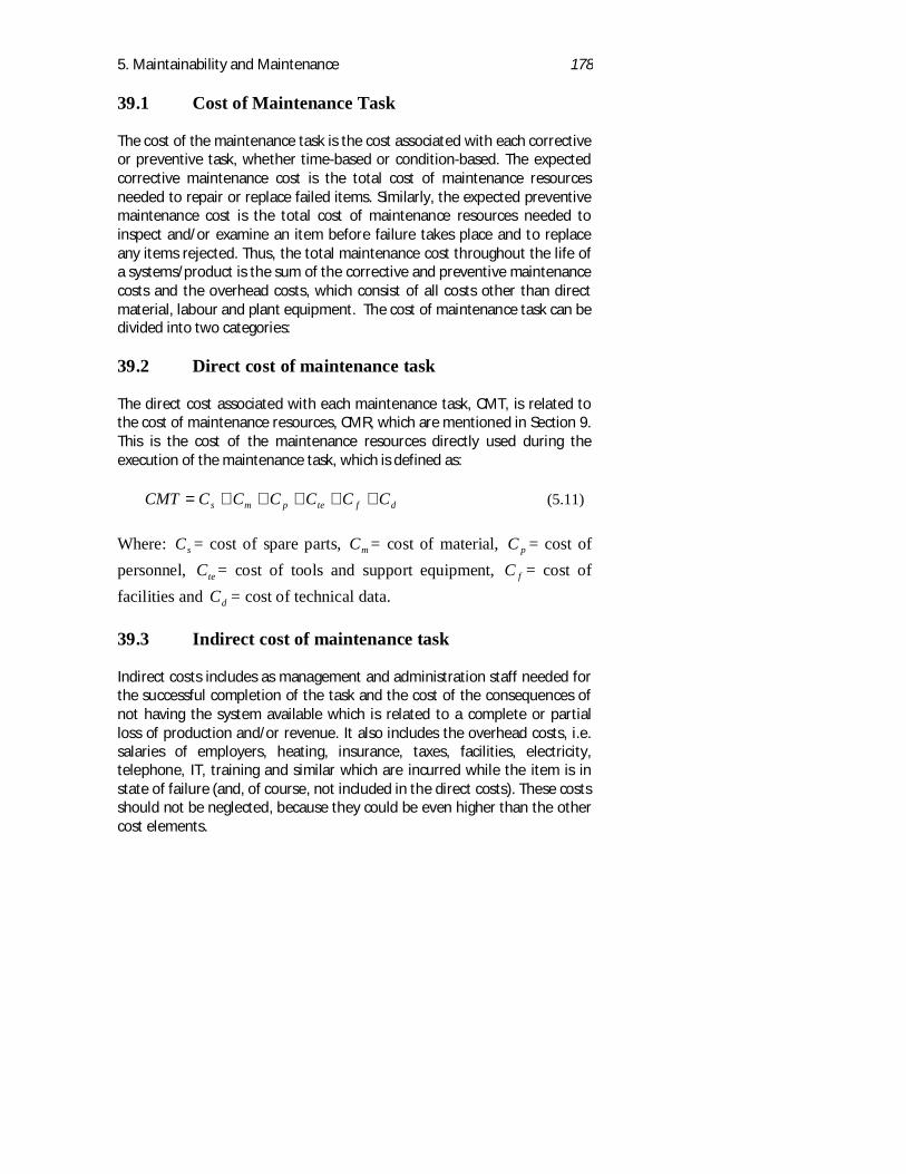
5. Maintainability and Maintenance 178
39.1 Cost of Maintenance Task
The cost of the maintenance task is the cost associated with each correctiveor preventive task, whether time-based or condition-based. The expectedcorrective maintenance cost is the total cost of maintenance resourcesneeded to repair or replace failed items. Similarly, the expected preventivemaintenance cost is the total cost of maintenance resources needed toinspect and/or examine an item before failure takes place and to replaceany items rejected. Thus, the total maintenance cost throughout the life ofa systems/product is the sum of the corrective and preventive maintenancecosts and the overhead costs, which consist of all costs other than directmaterial, labour and plant equipment. The cost of maintenance task can bedivided into two categories:
39.2 Direct cost of maintenance task
The direct cost associated with each maintenance task, CMT, is related tothe cost of maintenance resources, CMR, which are mentioned in Section 9.This is the cost of the maintenance resources directly used during theexecution of the maintenance task, which is defined as:
dftepms CCCCCCCMT +++++= (5.11)
Where: sC = cost of spare parts, mC = cost of material, pC = cost ofpersonnel, teC = cost of tools and support equipment, fC = cost offacilities and dC = cost of technical data.
39.3 Indirect cost of maintenance task
Indirect costs includes as management and administration staff needed forthe successful completion of the task and the cost of the consequences ofnot having the system available which is related to a complete or partialloss of production and/or revenue. It also includes the overhead costs, i.e.salaries of employers, heating, insurance, taxes, facilities, electricity,telephone, IT, training and similar which are incurred while the item is instate of failure (and, of course, not included in the direct costs). These costsshould not be neglected, because they could be even higher than the othercost elements.
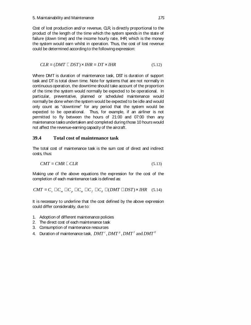
5. Maintainability and Maintenance 179
Cost of lost production and/or revenue, CLR, is directly proportional to theproduct of the length of the time which the system spends in the state offailure (down time) and the income hourly rate, IHR, which is the moneythe system would earn whilst in operation. Thus, the cost of lost revenuecould be determined according to the following expression:
IHRDTIHRDSTDMTCLR ×=×+= )( (5.12)
Where DMT is duration of maintenance task, DST is duration of supporttask and DT is total down time. Note for systems that are not normally incontinuous operation, the downtime should take account of the proportionof the time the system would normally be expected to be operational. Inparticular, preventative, planned or scheduled maintenance wouldnormally be done when the system would be expected to be idle and wouldonly count as “downtime” for any period that the system would beexpected to be operational. Thus, for example, if an airliner is notpermitted to fly between the hours of 21:00 and 07:00 then anymaintenance tasks undertaken and completed during those 10 hours wouldnot affect the revenue-earning capacity of the aircraft.
39.4 Total cost of maintenance task
The total cost of maintenance task is the sum cost of direct and indirectcosts, thus:
CMT CMR CLR= + (5.13)
Making use of the above equations the expression for the cost of thecompletion of each maintenance task is defined as:
IHRDSTDMTCCCCCCCMT dftepms ×+++++++= )( (5.14)
It is necessary to underline that the cost defined by the above expressioncould differ considerably, due to:
1. Adoption of different maintenance policies2. The direct cost of each maintenance task3. Consumption of maintenance resources
4. Duration of maintenance task, EIpc DMTDMTDMTDMT and,,
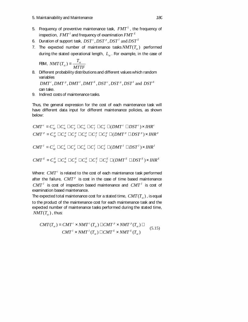
5. Maintainability and Maintenance 180
5. Frequency of preventive maintenance task, LFMT , the frequency of
inspection, IFMT and frequency of examination EFMT6. Duration of support task, EIpc DSTDSTDSTDST and,,7. The expected number of maintenance tasks NMT Tst( ) performed
during the stated operational length, stL . For example, in the case of
FBM,MTTF
TTNMT stst =)(
8. Different probability distributions and different values which randomvariables
EIpcEIpc DSTDSTDSTDSTDMTDMTDMTDMT and,,,,,,can take.
9. Indirect costs of maintenance tasks.
Thus, the general expression for the cost of each maintenance task willhave different data input for different maintenance policies, as shownbelow:
ccccd
cf
cte
cp
cm
csp
c IHRDSTDMTCCCCCCCMT ×+++++++= )(pppp
dpf
pte
pp
pm
psp
p IHRDSTDMTCCCCCCCMT ×+++++++= )(
IIIId
If
Ite
Ip
Im
Isp
I IHRDSTDMTCCCCCCCMT ×+++++++= )(
EEEEd
Ef
Ete
Ep
Em
Esp
E IHRDSTDMTCCCCCCCMT ×+++++++= )(
Where: CMT c is related to the cost of each maintenance task performed
after the failure, CMT p is cost in the case of time based maintenanceICMT is cost of inspection based maintenance and ICMT is cost of
examination based maintenance.The expected total maintenance cost for a stated time, )( stTCMT , is equal
to the product of the maintenance cost for each maintenance task and theexpected number of maintenance tasks performed during the stated time,NMT Tst( ) , thus:
)()(
)()()(
stEE
stII
stpp
stcc
st
TNMTCMTTNMTCMTTNMTCMTTNMTCMTTCMT
×+×
+×+×= (5.15)
5. Maintainability and Maintenance 181
39.5 Factor Affecting Maintenance Costs
Maintenance cost could be affected by the following factors:
1. Supply responsiveness or the probability of having a spare part availablewhen needed, supply lead times for given items, levels of inventory, andso on.
2. Test and support equipment effectiveness, which is the reliability andavailability of test equipment, test equipment utilisation, system testthoroughness, and so on.
3. Maintenance facility availability and utilisation.4. Transportation times between maintenance facilities.5. Maintenance organisational effectiveness and personnel efficiency.6. Durability and reliability of items in the system7. Life expectancy of system8. Expected number of maintenance tasks9. Duration of maintenance and support task10.Maintenance task resourcesIn order to reduce maintenance costs, it is necessary that the impact of theabove factors should be reduced and/or controlled.In calculating the various cost elements of maintenance, it is important torecognise that facilities, equipment, and personnel may be used for othertasks. For example, mechanics in the armed forces may be put on guardduty or provide a defence role when not performing maintenance tasks.Thus eliminating all maintenance tasks at first line (or O-Level) may notnecessarily lead to a significant reduction in the personnel deployed or,indeed, in the operational costs.
40. AIRCRAFT MAINTENANCE - CASE STUDY
For every commercial airline, maintenance is one of the most importantfunctions to assure safe operation. Federal Aviation Regulation (FAR)require that, no person may operate an aircraft unless the mandatoryreplacement times, inspection intervals and related procedures oralternative inspection intervals and related procedures set forth in theoperations specifications or inspection program has been complied with. Allaircraft must follow a maintenance program that is approved by aregulatory authority such as FAA (Federal Aviation Administration, USA) andCAA (Civil Aviation Authority, UK). Each airline develops its ownmaintenance plan, based on the manufacturer’s recommendations and by
5. Maintainability and Maintenance 182
considering its own operation. Thus, two different airlines may haveslightly different maintenance program for same aircraft model used undersimilar operating conditions. Aircraft maintenance is reliability centred. It isclaimed that each aircraft receives approximately 14 hours of maintenancefor every hour it flies (R Baker, 1995). Maintenance accounts forapproximately 10% of an airline’s total costs. On average a typical Boeing747 will generate a total aircraft maintenance cost of approximately $1,700per block hour.
Aircraft maintenance can be categorised as:
1. Routine scheduled maintenance.2. Non-routine maintenance.3. Refurbishment.4. Modifications.
Routine Scheduled Maintenance
Scheduled maintenance tasks are required at determinant recurringintervals or due to Airworthiness Directives (AD). The most commonroutine maintenance is visual inspection of the aircraft prior to a scheduleddeparture (known as walk around) by pilots and mechanics to ensure thatthere are no obvious problems. Routine maintenance can be classified as:
1. Overnight maintenance.2. Hard time maintenance.3. Progressive Inspection.
Overnight maintenance normally includes low level maintenance checks,minor servicing and special inspections done at the end of the working forabout one to two hours to ensure that the plane is operating in accordancewith Minimum Equipment List. Overnight maintenance provides anopportunity to remedy passenger and crew complaints (M Lam, 1995).Hard time is the oldest primary maintenance process. Hard time requiresperiodic overhaul or replacement of affected systems/components andstructures and is flight, cycle and calendar limited. That is, as soon as the
5. Maintainability and Maintenance 183
component age reaches it hard time it is replaced with a new component.Most of the rotating engine units are hard timed. The purpose of hard timemaintenance is to assure operating safety of component or system, whichhave a limited redundancy.Progressive inspection groups like time related maintenance tasks intoconvenient ‘blocks’ so that maintenance workload becomes balanced withtime and maintenance can be accomplished in small ‘bites’ makingequipment more available. Grouping maintenance tasks also helps betterutilisation of the maintenance facilities. These maintenance task groups are(detailed information can be found in M Lam (1995) and L R Crawford,1995):1. Pre-flight Visual inspections carried out by the mechanic and the pilots
to ensure that there are no obvious problems.2. A Check Carried out approximately every 150 flight hours, which
includes selected operational checks (general inspection of theinterior/exterior of the aircraft), fluid servicing, extended visualinspection of fuselage exterior, power supply and certain operationaltasks. During A check, the aircraft is on ground for approximately 8 to10 hours and requires approximately 60 labour hours.
3. B Check Occurs about every 750 flight hours and includes somepreventive maintenance such as engine oil spectro-analysis, oil-filter areremoved and checked, lubrication of parts as required and examination ofairframe. Also incorporates A-check. The aircraft could be on ground for10 hours and will require approximately 200 labour hours.
4. C Check Occurs every 3, 000 flight hour (approximately 15 months)and includes detailed inspection of airframe, engines, and accessories. Inaddition, components are repaired, flight controls are calibrated, andmajor internal mechanisms are tested. Functional and operational checksare also performed during C-check. It also includes both A and Bchecks. The aircraft will be on ground for 72 hours and will requireapproximately 3,000 labour hours.
5. D Check This is the most intensive form of routine maintenance occursabout 20,000 flight hours (six to eight years). It is an overhaul thatreturns the aircraft to its original condition, as far as possible. Cabininteriors including seats, galleys, furnishings etc are removed to allowcareful structural inspections. The aircraft is on ground for about 30 daysand will require approximately 20,000 labour hours.
A and B checks and overnight maintenance are instances of linemaintenance (performed upon the aircraft incidental to its scheduledrevenue operations), often carried out an airport. C and D checks, however
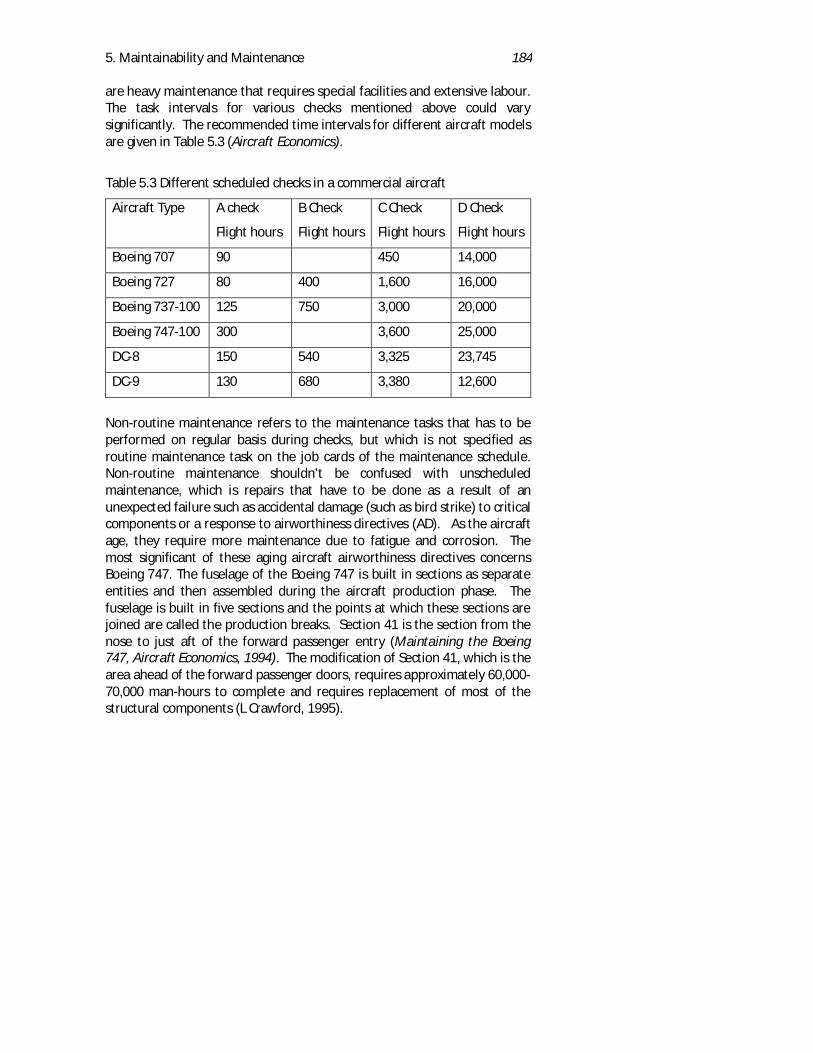
5. Maintainability and Maintenance 184
are heavy maintenance that requires special facilities and extensive labour.The task intervals for various checks mentioned above could varysignificantly. The recommended time intervals for different aircraft modelsare given in Table 5.3 (Aircraft Economics).
Table 5.3 Different scheduled checks in a commercial aircraft
Aircraft Type A check
Flight hours
B Check
Flight hours
C Check
Flight hours
D Check
Flight hours
Boeing 707 90 450 14,000
Boeing 727 80 400 1,600 16,000
Boeing 737-100 125 750 3,000 20,000
Boeing 747-100 300 3,600 25,000
DC-8 150 540 3,325 23,745
DC-9 130 680 3,380 12,600
Non-routine maintenance refers to the maintenance tasks that has to beperformed on regular basis during checks, but which is not specified asroutine maintenance task on the job cards of the maintenance schedule.Non-routine maintenance shouldn’t be confused with unscheduledmaintenance, which is repairs that have to be done as a result of anunexpected failure such as accidental damage (such as bird strike) to criticalcomponents or a response to airworthiness directives (AD). As the aircraftage, they require more maintenance due to fatigue and corrosion. Themost significant of these aging aircraft airworthiness directives concernsBoeing 747. The fuselage of the Boeing 747 is built in sections as separateentities and then assembled during the aircraft production phase. Thefuselage is built in five sections and the points at which these sections arejoined are called the production breaks. Section 41 is the section from thenose to just aft of the forward passenger entry (Maintaining the Boeing747, Aircraft Economics, 1994). The modification of Section 41, which is thearea ahead of the forward passenger doors, requires approximately 60,000-70,000 man-hours to complete and requires replacement of most of thestructural components (L Crawford, 1995).

5. Maintainability and Maintenance 185
5. Maintainability and Maintenance 186
Availability, Designfor Reliability andData AnalysisCourse Material
Course Instructor: Professor U Dinesh KumarIndian Institute of Management Bangalore
10. Availability 187
Chapter 10
AvailabilityThere is nothing in this world constant, but inconsistency
Jonathan Swift
Availability is used to measure the combined effect of reliability,maintenance and logistic support on the operational effectiveness of thesystem. A system, which is in a state of failure, is not beneficial to itsowner; in fact, it is probably costing the owner money. If an aircraft breaksdown, it cannot be used until it has been declared airworthy. This is likelyto cause inconvenience to the customers who may then decide to switch toan alternative airline in future. It may disrupt the timetables and causeproblems for several days.As mentioned in Chapter 9, most large airliners have a very high utilisationrate with the only down time being to do a transit check, unload, clean thecabin, refuel, restock with the next flight’s foods and other items, andreload with the next set of passengers and baggage. The whole operationgenerally takes about an hour. Any delay may cause it to miss its take offslot and more significantly its landing slot, since an aircraft cannot take-offuntil it has been cleared to land, even though this may be 12 hours later.Many airports close during the night to avoid unacceptable levels of noisepollution. If the particular flight was due to land just before the airportcloses, missing its slot could mean a delay of several hours.An operator of a system would like to make sure that the system will be in astate of functioning (SoFu) when it is required. Designers andmanufacturers know that they are unlikely to remain in business for verylong if their systems do not satisfy the customers’ requirements in terms ofoperational effectiveness. Many forms of availability are used to measurethe effectiveness of the system. Inherent availability, operationalavailability and achieved availability are some of the measures used to
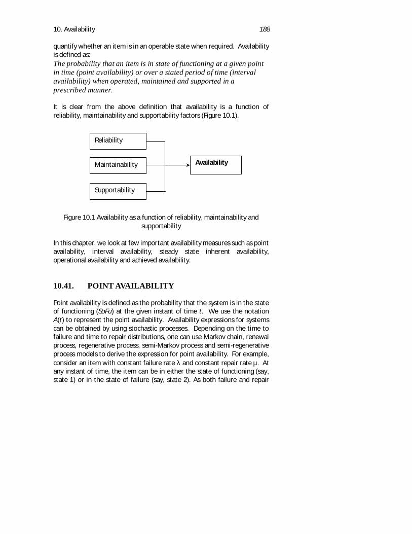
10. Availability 188
quantify whether an item is in an operable state when required. Availabilityis defined as:The probability that an item is in state of functioning at a given pointin time (point availability) or over a stated period of time (intervalavailability) when operated, maintained and supported in aprescribed manner.
It is clear from the above definition that availability is a function ofreliability, maintainability and supportability factors (Figure 10.1).
Figure 10.1 Availability as a function of reliability, maintainability andsupportability
In this chapter, we look at few important availability measures such as pointavailability, interval availability, steady state inherent availability,operational availability and achieved availability.
10.41. POINT AVAILABILITY
Point availability is defined as the probability that the system is in the stateof functioning (SoFu) at the given instant of time t. We use the notationA(t) to represent the point availability. Availability expressions for systemscan be obtained by using stochastic processes. Depending on the time tofailure and time to repair distributions, one can use Markov chain, renewalprocess, regenerative process, semi-Markov process and semi-regenerativeprocess models to derive the expression for point availability. For example,consider an item with constant failure rate λ and constant repair rate µ. Atany instant of time, the item can be in either the state of functioning (say,state 1) or in the state of failure (say, state 2). As both failure and repair
Reliability
Maintainability
Supportability
Availability
10. Availability 189
rates are constant (and thus follow exponential distribution), we can use aMarkov chain to model the system to derive the availability expression.
Let pij(h) denote the transition probability from state i to state j during theinterval ‘h’(i,j = 1, 2). Define, Pi(t+h), as the probability that the systemwould be in state i at time t+h, for i = 1, 2. The expression for P1(t+h) can bederived using the following logic:
1. The system was in state 1 at time t and continues to remain instate 1 throughout the interval h.
2. The system was in state 2 at time t and it transits to state 1 duringthe interval h.
The corresponding expression can be written as:
)()()()()( 2121111 tptPhptPhtP ×+×=+ (10.1)
Using similar logic, the expression for P2(t+h) can be written as:
)()()()()( 2221212 hptPhptPhtP ×+×=+ (10.2)
p11(h) is the probability of remaining in state 1 during the interval h. Theprobability p11(h) is given by
1)exp()(11 hhhp λλ −≈−= for λh<<1
p21(h) is the probability of entering state 1 from state 2 during the intervalh. The corresponding expression is given by
hhhp µµ ≈−−= )exp(1)(21 for hµ<<1
p12(h) is the probability of entering state 2 from state 1 during the intervalh. The probability p12(h) is given by
hhhp λλ ≈−−= )exp(1)(12 for hλ<<1
p22(h) is the probability of remaining in state 2 during the interval h. Theprobability p22(h) is given by:
hhhp µµ −≈−= 1)exp()(22 for hµ<<1
10. Availability 190
Substituting the values of pij(h) in equation (10.1) and (10.2), we get
htPhtPhtP µλ ×+−×=+ )()1()()( 211
)1()()()()( 212 htPhtPhtP µλ −×+×=+
By rearranging the terms and setting h → 0, we have
)()()()()(
21111
0tPtP
dttdP
htPhtP
Lth
µλ +−==−+
→
)()()()()(
21222
0tPtP
dttdP
htPhtP
Lth
µλ −==−+
→
On solving the above two differential equations, we get
))(exp()(1 ttP µλµλ
λµλ
µ+−×
++
+=
P1(t) is nothing but the availability of the item at time t, that is theprobability that the item will be in state of functioning at time t. Thus, thepoint availability A(t) is given by:
))(exp()( ttA µλµλ
λµλ
µ+−×
++
+= (10.3)
Substituting λ = 1/MTTF and µ = 1/MTTR in the above equation, we get
))11(exp()( tMTTRMTTFMTTRMTTF
MTTRMTTRMTTF
MTTFtA +−×+
++
= (10.4)
When the time to failure and time to repair are not exponential, we can usea regenerative process to derive the availability expression. If f(t) and g(t)represent the time-to-failure and time-to-repair distributions respectively,then the point availability A(t) can be written as (Birolini, 1997):
dxxtFxgxftFtAt
n
n)](1[)](*)([)(1)(
0 1−−+−= ∫ ∑
∞
=
10. Availability 191
where [f(x)*g(x)]n is the n-fold convolution of f(x)*g(x). The summation
∑∞
=∗
1)]()([
n
nxgxf gives the renewal points f(x)*g(x), f(x)*g(x)*f(x)*g(x),
lies in [x, x+dx], and 1 F(t-x) is the probability that no failures occur in theremaining interval [x, t].
10.41.1 Average Availability
Interval availability, AA(t), is defined as the expected fractional duration ofan interval (0, t] that the system is in state of functioning. Thus,
∫=t
dxxAt
tAA0
)(1)( (10.5)
where A(x) is the point availability of the item as defined in equation (10.3)and (10.4). For an item with constant failure rate λ and constant repair rateµ, the average availability is given by:
)])(exp(1[)(
)( 2 tt
tAA µλµλ
λµλ
µ+−−
++
+= (10.6)
10.41.2 Inherent Availability
Inherent availability (or steady-state availability), Ai,, is defined as thesteady state probability (that is, t → ∞) that an item will be in a state offunctioning, assuming that this probability depends only on the time-to-failure and time to repair distributions. It is assumed that any supportresources that are required are available without any restriction. Thus, theinherent availability is given by:
MTTRMTTFMTTFtALtA
ti +
==∞→
)( (10.7)
The above result is valid for any time to failure function F(t) and any time torepair distribution G(t) (Birolini, 1997). Also, in the case of constant failurerate λ and constant repair rate µ, the following inequality is true.
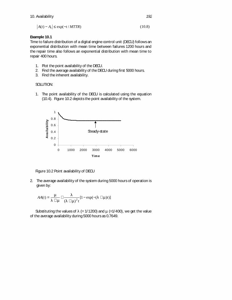
10. Availability 192
)/exp()( MTTRtAtA i −≤− (10.8)
Example 10.1Time to failure distribution of a digital engine control unit (DECU) follows anexponential distribution with mean time between failures 1200 hours andthe repair time also follows an exponential distribution with mean time torepair 400 hours.
1. Plot the point availability of the DECU.2. Find the average availability of the DECU during first 5000 hours.3. Find the inherent availability.
SOLUTION:
1. The point availability of the DECU is calculated using the equation(10.4). Figure 10.2 depicts the point availability of the system.
Figure 10.2 Point availability of DECU
2. The average availability of the system during 5000 hours of operation isgiven by:
)])(exp(1[)(
)( 2 tt
tAA µλµλ
λµλ
µ+−−
++
+=
Substituting the values of λ (= 1/1200) and µ (=1/400), we get the valueof the average availability during 5000 hours as 0.7649.
0
0.2
0.4
0.6
0.8
1
0 1000 2000 3000 4000 5000 6000
Time
Ava
ilabi
lity
Steady-state
10. Availability 193
3. The inherent availability is given by
75.04001200
1200=
+=
+=
MTTRMTTFMTTFAi
Thus, the steady state availability of the system is 0.75 or 75%.
10.41.3 System Availability of different reliability blockdiagrams
Availability of a system with series reliability block diagram with n items isgiven by
)()(1
tAtAn
kis ∏
== (10.9)
where Ai(t) is the point availability of ith item. The inherent availability ofthe system is given by
∏= +
=n
k ii
isi MTTRMTTF
MTTFA
1, (10.10)
For a series system with all the elements having constant failure and repairrates, the system inherent availability
ss
ssi MTTRMTTF
MTTFA
+=, (10.11)
MTTFs and MTTRs are system mean time to failure and system mean time torepair respectively. Let λi and µi represent the failure rate and repair rateof item i respectively. MTTFs and MTTRs are given by
∑=
= n
ii
sMTTF
1
1
λ
∑=
=n
i s
iis
MTTRMTTR1 λλ
, where ∑=
=n
iis
1λλ
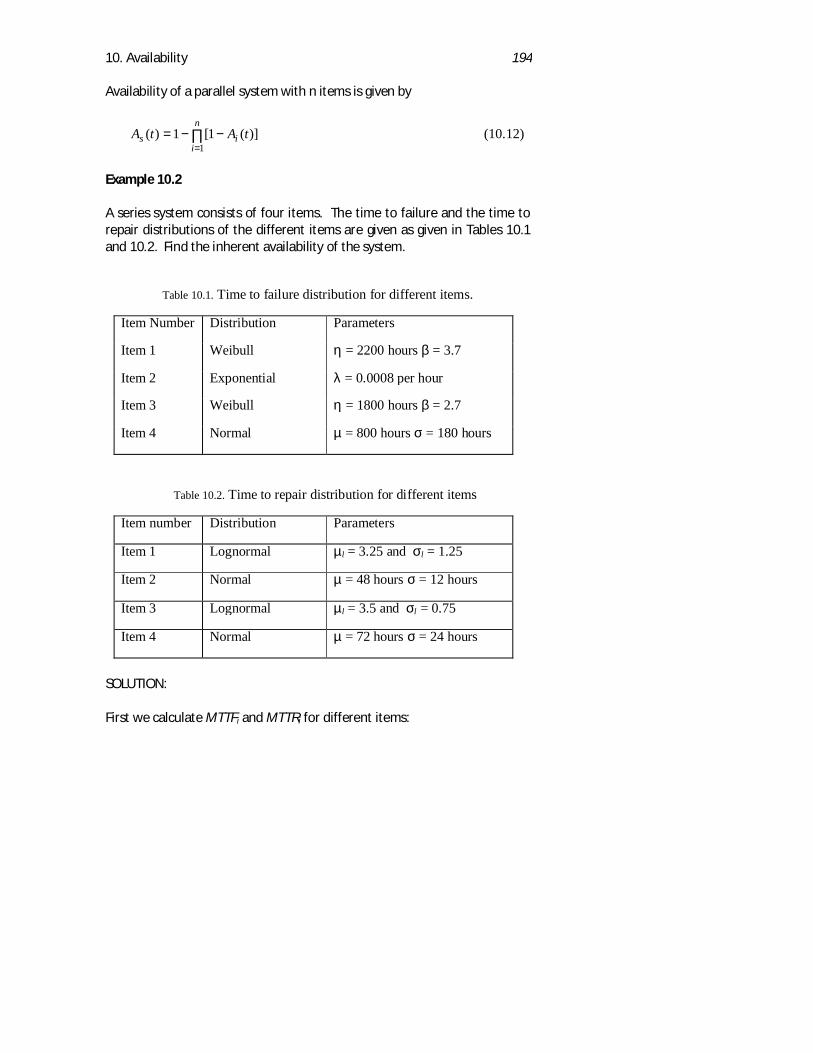
10. Availability 194
Availability of a parallel system with n items is given by
∏=
−−=n
iis tAtA
1)](1[1)( (10.12)
Example 10.2
A series system consists of four items. The time to failure and the time torepair distributions of the different items are given as given in Tables 10.1and 10.2. Find the inherent availability of the system.
Table 10.1. Time to failure distribution for different items.
Item Number Distribution Parameters
Item 1 Weibull η = 2200 hours β = 3.7
Item 2 Exponential λ = 0.0008 per hour
Item 3 Weibull η = 1800 hours β = 2.7
Item 4 Normal µ = 800 hours σ = 180 hours
Table 10.2. Time to repair distribution for different items
Item number Distribution Parameters
Item 1 Lognormal µl = 3.25 and σl = 1.25
Item 2 Normal µ = 48 hours σ = 12 hours
Item 3 Lognormal µl = 3.5 and σl = 0.75
Item 4 Normal µ = 72 hours σ = 24 hours
SOLUTION:
First we calculate MTTFi and MTTRi for different items:
10. Availability 195
4.1984902.02200)7.3
11(2200)11(1 =×=+Γ×=+Γ×=β
ηMTTF
12500008.0/1/12 === λMTTF , 2.16003 =MTTF , MTTF4 =800
33.56)2/exp( 21 =+= llMTTR σµ hours, MTTR2 =48 hours
87.43)2/exp( 23 =+= llMTTR σµ hours, MTTR4 = 72 hours
Inherent availability, Ai, for item i can be calculated using the equation(10.11). Substituting the values of MTTFi and MTTRi in equation (10.11), wehave
A1 = 0.9723, A2 = 0.9630, A3 = 0.9733, A4 = 0.9174
The system availability is given by
8362.04
1== ∏
=iis AA
10.42. ACHIEVED AVAILABILITY
Achieved availability is the probability that an item will be in a state offunctioning (SoFu) when used as specified taking into account thescheduled and unscheduled maintenance; any support resources neededare available instantaneously. Achieved availability, Aa, is given by
AMTMTBMMTBMAa +
= (10.13)
MTBM is the mean time between maintenance and AMT is activemaintenance time. The mean time between maintenance during the totaloperational life, T, is given by:
smTTTMTMTBM
/)( += (10.14)
M(T) is the renewal function, that is the expected number of failures duringthe total life T. Tsm is the scheduled maintenance interval (time betweenscheduled maintenance). The above expression is valid when after eachscheduled maintenance, the item is ‘as-bad-as-old’ and after each
10. Availability 196
corrective maintenance the item is ‘as-good-as-new’. The activemaintenance time, AMT, is given by:
sm
sm
TTTMMSMTTTMTTRTM
AMT/)(
)/()(++×
= (10.15)
MTTR stands for the mean time to repair and MSMT is the mean scheduledmaintenance time.
Example 10.3
Time to failure distribution of an engine monitoring system follows anormal distribution with mean 4200 hours and standard deviation 420hours. The engine monitoring system is expected to last 20,000 hours(subject to corrective and preventive maintenance). A scheduledmaintenance is carried out after every 2000 hours and takes about 72hours to complete the task. The time to repair the item follows alognormal distribution with mean time to repair 120 hours. Find theachieved availability for this system.
SOLUTION:
Mean time between maintenance, MTBM, is given by
2000/20000)20000(20000
/)( +=
+=
MTTTMTMTBM
sm
M(20000) for normal distribution with mean 4200 hours and standarddeviation 420 hours is given by
1434.4)420
420020000()20000(1
=×
×−Φ= ∑
∞
= nnM
n
hours1414101434.4
20000≈
+=MTBM
The active maintenance time is given by:
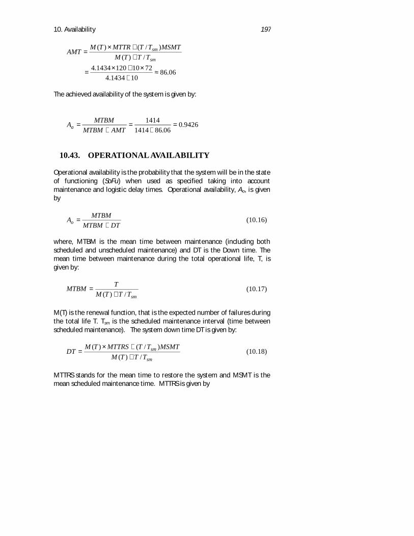
10. Availability 197
06.86101434.4
72101201434.4/)(
)/()(
≈+
×+×=
++×
=sm
sm
TTTMMSMTTTMTTRTM
AMT
The achieved availability of the system is given by:
9426.006.861414
1414=
+=
+=
AMTMTBMMTBMAa
10.43. OPERATIONAL AVAILABILITY
Operational availability is the probability that the system will be in the stateof functioning (SoFu) when used as specified taking into accountmaintenance and logistic delay times. Operational availability, Ao, is givenby
DTMTBMMTBMAo +
= (10.16)
where, MTBM is the mean time between maintenance (including bothscheduled and unscheduled maintenance) and DT is the Down time. Themean time between maintenance during the total operational life, T, isgiven by:
smTTTMTMTBM
/)( += (10.17)
M(T) is the renewal function, that is the expected number of failures duringthe total life T. Tsm is the scheduled maintenance interval (time betweenscheduled maintenance). The system down time DT is given by:
sm
sm
TTTMMSMTTTMTTRSTM
DT/)(
)/()(++×
= (10.18)
MTTRS stands for the mean time to restore the system and MSMT is themean scheduled maintenance time. MTTRS is given by
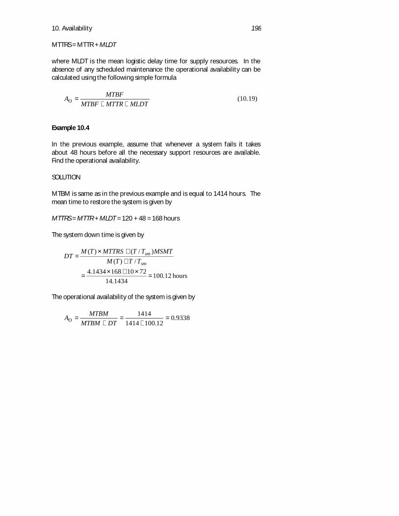
10. Availability 198
MTTRS = MTTR + MLDT
where MLDT is the mean logistic delay time for supply resources. In theabsence of any scheduled maintenance the operational availability can becalculated using the following simple formula
MLDTMTTRMTBFMTBFAO ++
= (10.19)
Example 10.4
In the previous example, assume that whenever a system fails it takesabout 48 hours before all the necessary support resources are available.Find the operational availability.
SOLUTION
MTBM is same as in the previous example and is equal to 1414 hours. Themean time to restore the system is given by
MTTRS = MTTR + MLDT = 120 + 48 = 168 hours
The system down time is given by
hours12.1001434.14
72101681434.4/)(
)/()(
=×+×
=
++×
=sm
sm
TTTMMSMTTTMTTRSTM
DT
The operational availability of the system is given by
9338.012.1001414
1414=
+=
+=
DTMTBMMTBMAO
11. Design for Reliability, Maintenance and Logistic Support 199
Chapter 11
Design for Reliability, Maintenance andLogistic Support
Reliability, maintenance and supportability should be designed into theproduct. Design phase is particularly important for any product as thedecisions made during this stage can determine how reliable the product isgoing to be as well as the maintainability and supportability of that product.In this chapter, we would like to discuss few tool and techniques that canbe used at the design stage to improve the RMS characteristics.
44. RELIABILITY ALLOCATION
Reliability allocation is a process by which the system’s reliabilityrequirements is divided into sub-system and component reliabilityrequirements.
45. FAILURE MODES, EFFECTS AND CRITICALITYANALYSIS (FMECA)
The failure modes, effects and criticality analysis (FMECA) is a systematicmethod for examining all modes through which a failure can occur,
11. Design for Reliability, Maintenance and Logistic Support 200
potential effects of these failures on the system performance and theirrelative severity in terms of safety, extend of damage, and impact onmission success. FMECA is performed to identify reliability, maintenance,safety and supportability problems resulting from the effects of aproduct/process failure. It is an excellent methodology for identifying andinvestigating potential product weaknesses. FMECA establishes a detailedstudy of the product design, manufacturing operation or distribution todetermine which features are critical to various modes of failure. TheFMECA concept was developed by US defence industries in the 1950s, toimprove the reliability of military equipment. Since then, FMECA hasbecome an important tools applied by almost all industries around theworld to improve the reliability, maintainability and supportability of theirproduct. It is claimed that a more rigorous FMECA analysis would haveavoided the disastrous explosion of the Challenger launch on 28th January1986.
The three principal study areas in FMECA analysis are the failure mode,failure effect and failure criticality. Failure mode analysis lists all possiblemode the failure would occur which include the condition, the componentsinvolved, location etc. The failure effect analysis includes the study of thelikely impact of failure on the performance of the whole product and theprocess. The criticality analysis examines how critical a failure would be forthe operation and safe use of the product. The criticality might range fromminor failure through lowering of performance, shutdown of the product,safety and environmental hazard to a catastrophic failure. This analysis isbest utilised during the early design and development phase of newsystems, and in the evaluation of existing system (D Verma, 1993).
The actual FMECA performed could be both quantitative and qualitativebased on the information available to the analyst. Input requirements forFMECA analysis include reliability data, their modes of failure, and theestimated criticality of the failures. Additionally, the probabilities ofdetection for the various failure modes are also required. A prerequisite forthe successful completion of FMECA is good knowledge of, and familiaritywith the product/process being analysed and its design and functionality (DVerma, 1993).
45.1 Procedural Steps in the FMECA analysis
The procedural steps in FMECA analysis depend to a certain extend whatproduct or process is being examined. The sequence of steps followed to
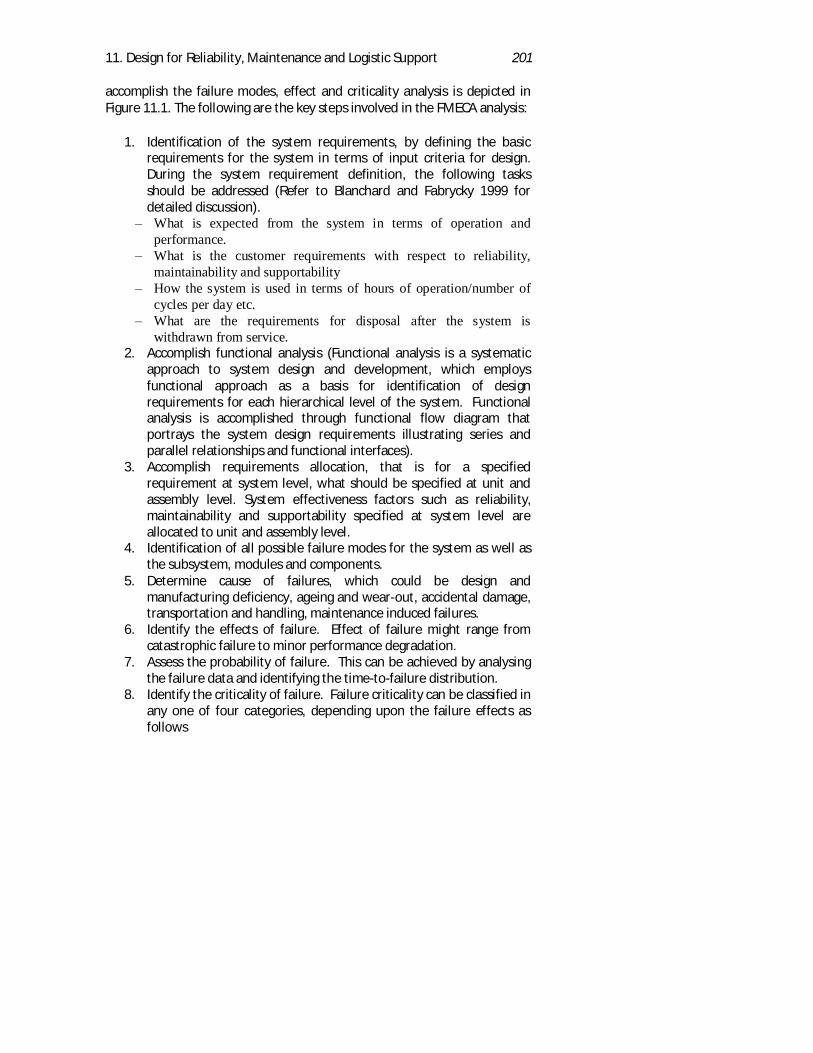
11. Design for Reliability, Maintenance and Logistic Support 201
accomplish the failure modes, effect and criticality analysis is depicted inFigure 11.1. The following are the key steps involved in the FMECA analysis:
1. Identification of the system requirements, by defining the basicrequirements for the system in terms of input criteria for design.During the system requirement definition, the following tasksshould be addressed (Refer to Blanchard and Fabrycky 1999 fordetailed discussion).
What is expected from the system in terms of operation andperformance.What is the customer requirements with respect to reliability,maintainability and supportabilityHow the system is used in terms of hours of operation/number ofcycles per day etc.What are the requirements for disposal after the system iswithdrawn from service.
2. Accomplish functional analysis (Functional analysis is a systematicapproach to system design and development, which employsfunctional approach as a basis for identification of designrequirements for each hierarchical level of the system. Functionalanalysis is accomplished through functional flow diagram thatportrays the system design requirements illustrating series andparallel relationships and functional interfaces).
3. Accomplish requirements allocation, that is for a specifiedrequirement at system level, what should be specified at unit andassembly level. System effectiveness factors such as reliability,maintainability and supportability specified at system level areallocated to unit and assembly level.
4. Identification of all possible failure modes for the system as well asthe subsystem, modules and components.
5. Determine cause of failures, which could be design andmanufacturing deficiency, ageing and wear-out, accidental damage,transportation and handling, maintenance induced failures.
6. Identify the effects of failure. Effect of failure might range fromcatastrophic failure to minor performance degradation.
7. Assess the probability of failure. This can be achieved by analysingthe failure data and identifying the time-to-failure distribution.
8. Identify the criticality of failure. Failure criticality can be classified inany one of four categories, depending upon the failure effects asfollows
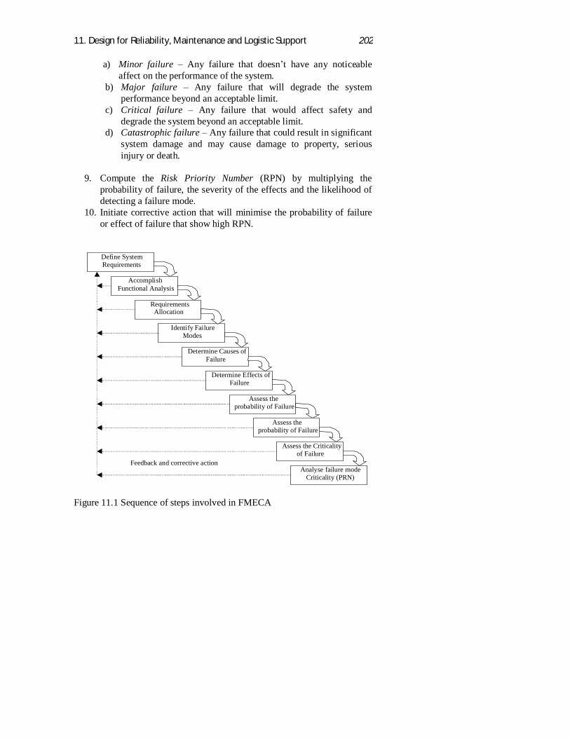
11. Design for Reliability, Maintenance and Logistic Support 202
a) Minor failure Any failure that doesn t have any noticeableaffect on the performance of the system.
b) Major failure Any failure that will degrade the systemperformance beyond an acceptable limit.
c) Critical failure Any failure that would affect safety anddegrade the system beyond an acceptable limit.
d) Catastrophic failure Any failure that could result in significantsystem damage and may cause damage to property, seriousinjury or death.
9. Compute the Risk Priority Number (RPN) by multiplying theprobability of failure, the severity of the effects and the likelihood ofdetecting a failure mode.
10. Initiate corrective action that will minimise the probability of failureor effect of failure that show high RPN.
Figure 11.1 Sequence of steps involved in FMECA
Define SystemRequirements
AccomplishFunctional Analysis
RequirementsAllocation
Identify FailureModes
Determine Causes ofFailure
Determine Effects ofFailure
Assess theprobability of Failure
Assess theprobability of Failure
Assess the Criticalityof Failure
Analyse failure modeCriticality (PRN)
Feedback and corrective actionloop
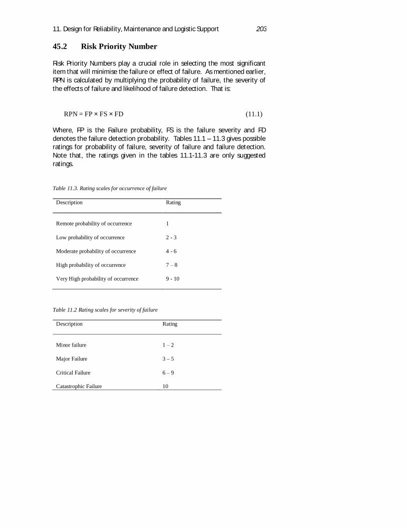
11. Design for Reliability, Maintenance and Logistic Support 203
45.2 Risk Priority Number
Risk Priority Numbers play a crucial role in selecting the most significantitem that will minimise the failure or effect of failure. As mentioned earlier,RPN is calculated by multiplying the probability of failure, the severity ofthe effects of failure and likelihood of failure detection. That is:
RPN = FP × FS × FD (11.1)
Where, FP is the Failure probability, FS is the failure severity and FDdenotes the failure detection probability. Tables 11.1 – 11.3 gives possibleratings for probability of failure, severity of failure and failure detection.Note that, the ratings given in the tables 11.1-11.3 are only suggestedratings.
Table 11.3. Rating scales for occurrence of failure
Description Rating
Remote probability of occurrence 1
Low probability of occurrence 2 - 3
Moderate probability of occurrence 4 - 6
High probability of occurrence 7 8
Very High probability of occurrence 9 - 10
Table 11.2 Rating scales for severity of failure
Description Rating
Minor failure 1 2
Major Failure 3 5
Critical Failure 6 9
Catastrophic Failure 10
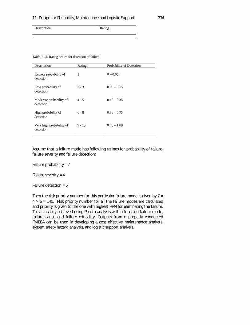
11. Design for Reliability, Maintenance and Logistic Support 204
Description Rating
Table 11.3. Rating scales for detection of failure
Description Rating Probability of Detection
Remote probability ofdetection
1 0 0.05
Low probability ofdetection
2 - 3 0.06 0.15
Moderate probability ofdetection
4 - 5 0.16 0.35
High probability ofdetection
6 - 8 0.36 0.75
Very high probability ofdetection
9 - 10 0.76 1.00
Assume that a failure mode has following ratings for probability of failure,failure severity and failure detection:
Failure probability = 7
Failure severity = 4
Failure detection = 5
Then the risk priority number for this particular failure mode is given by 7 ×4 × 5 = 140. Risk priority number for all the failure modes are calculatedand priority is given to the one with highest RPN for eliminating the failure.This is usually achieved using Pareto analysis with a focus on failure mode,failure cause and failure criticality. Outputs from a properly conductedFMECA can be used in developing a cost effective maintenance analysis,system safety hazard analysis, and logistic support analysis.
11. Design for Reliability, Maintenance and Logistic Support 205
46. FAULT TREE ANALYSIS (FTA)
Fault tree analysis is a deductive approach involving graphical enumerationand analysis of the different ways in which a particular system failure canoccur, and the probability of its occurrence. It starts with a top-level event(failure) and works backward to identify all the possible causes andtherefore the origins of that failure. During the very early stages of systemdesign process, and in the absence of information required to complete aFMECA, fault tree analysis (FTA) is often conducted to gain insight intocritical aspects of selected design concepts. Usually, a separate fault tree isdeveloped for every critical failure mode or undesired Top-Level event.Attention is focused on this top-level event and the first-tier causesassociated with it. Each first-tier cause is next investigated for its causes,and this process is continued. This ‘Top-Down’ causal hierarchy and theassociated probabilities, is called a Fault Tree.
One of the outputs from a fault tree analysis is the probability of occurrenceof the top-level event or failure. If this probability is unacceptable, faulttree analysis provides the designers with an insight into aspects of thesystem to which redesign can be directed or compensatory provisions beprovided such as redundancy. The FTA can have most impact if initiatedduring the conceptual and preliminary design phase when design andconfiguration changes can be most easily and cost effectively implemented.
The logic used in developing and analysing a fault tree has its foundations inBoolean Algebra. The following steps are used to carry out FTA (Figure11.2).
1. Identify the top-level event The most important step is to identify anddefine the top-level event. It is necessary to specific in defining the top-level event, a generic and non-specific definition is likely to result in abroad based fault tree which might be lacking in focus.
2. Develop the initial fault tree Once the top-level event has beensatisfactorily identified, the next step is to construct the initial causalhierarchy in the form of a fault tree. Techniques such as Ishikawa scause and effect diagram can prove beneficial. While developing thefault tree all hidden failures must be considered and incorporated. For thesake of consistency, a standard symbol is used to develop fault trees.Table 11.4 depicts the symbols used to represent the causal hierarchy andinterconnects associated with a particular top-level event. While
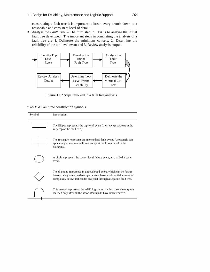
11. Design for Reliability, Maintenance and Logistic Support 206
constructing a fault tree it is important to break every branch down to areasonable and consistent level of detail.
3. Analyse the Fault Tree The third step in FTA is to analyse the initialfault tree developed. The important steps in completing the analysis of afault tree are 1. Delineate the minimum cut-sets, 2. Determine thereliability of the top-level event and 3. Review analysis output.
Figure 11.2 Steps involved in a fault tree analysis.
Table 11.4. Fault tree construction symbols
Symbol Description
The Ellipse represents the top-level event (thus always appears at thevery top of the fault tree).
The rectangle represents an intermediate fault event. A rectangle canappear anywhere in a fault tree except at the lowest level in thehierarchy.
A circle represents the lowest level failure event, also called a basicevent.
The diamond represents an undeveloped event, which can be furtherbroken. Very often, undeveloped events have a substantial amount ofcomplexity below and can be analysed through a separate fault tree.
This symbol represents the AND logic gate. In this case, the output isrealised only after all the associated inputs have been received.
Identify TopLevelEvent
Develop theInitial
Fault Tree
Analyse theFaultTree
Delineate theMinimal Cut-
sets
Determine Top-Level EventReliability
Review AnalysisOutput
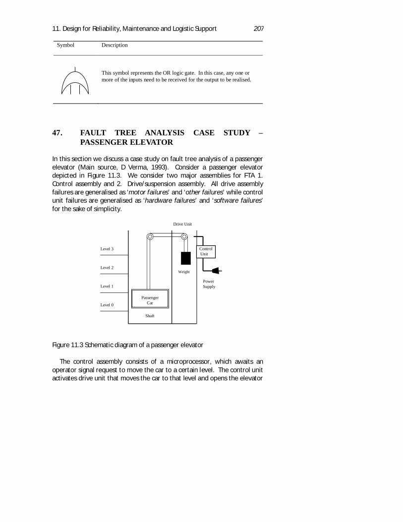
11. Design for Reliability, Maintenance and Logistic Support 207
Symbol Description
This symbol represents the OR logic gate. In this case, any one ormore of the inputs need to be received for the output to be realised.
47. FAULT TREE ANALYSIS CASE STUDYPASSENGER ELEVATOR
In this section we discuss a case study on fault tree analysis of a passengerelevator (Main source, D Verma, 1993). Consider a passenger elevatordepicted in Figure 11.3. We consider two major assemblies for FTA 1.Control assembly and 2. Drive/suspension assembly. All drive assemblyfailures are generalised as ‘motor failures’ and ‘other failures’ while controlunit failures are generalised as ‘hardware failures’ and ‘software failures’for the sake of simplicity.
Figure 11.3 Schematic diagram of a passenger elevator
The control assembly consists of a microprocessor, which awaits anoperator signal request to move the car to a certain level. The control unitactivates drive unit that moves the car to that level and opens the elevator
PassengerCar
Shaft
Level 3
Level 2
Level 1
Level 0
Drive Unit
Control Unit
PowerSupply
Weight
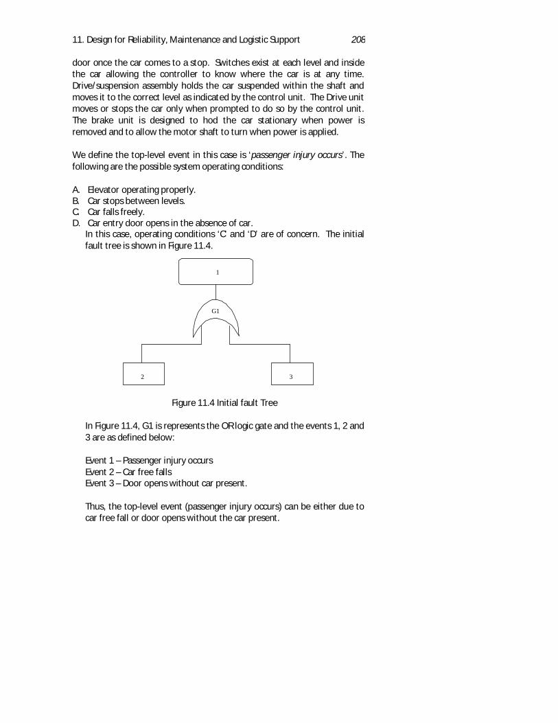
11. Design for Reliability, Maintenance and Logistic Support 208
door once the car comes to a stop. Switches exist at each level and insidethe car allowing the controller to know where the car is at any time.Drive/suspension assembly holds the car suspended within the shaft andmoves it to the correct level as indicated by the control unit. The Drive unitmoves or stops the car only when prompted to do so by the control unit.The brake unit is designed to hod the car stationary when power isremoved and to allow the motor shaft to turn when power is applied.
We define the top-level event in this case is ‘passenger injury occurs’. Thefollowing are the possible system operating conditions:
A. Elevator operating properly.B. Car stops between levels.C. Car falls freely.D. Car entry door opens in the absence of car.
In this case, operating conditions ‘C’ and ‘D’ are of concern. The initialfault tree is shown in Figure 11.4.
Figure 11.4 Initial fault Tree
In Figure 11.4, G1 is represents the OR logic gate and the events 1, 2 and3 are as defined below:
Event 1 – Passenger injury occursEvent 2 – Car free fallsEvent 3 – Door opens without car present.
Thus, the top-level event (passenger injury occurs) can be either due tocar free fall or door opens without the car present.
1
2 3
G1
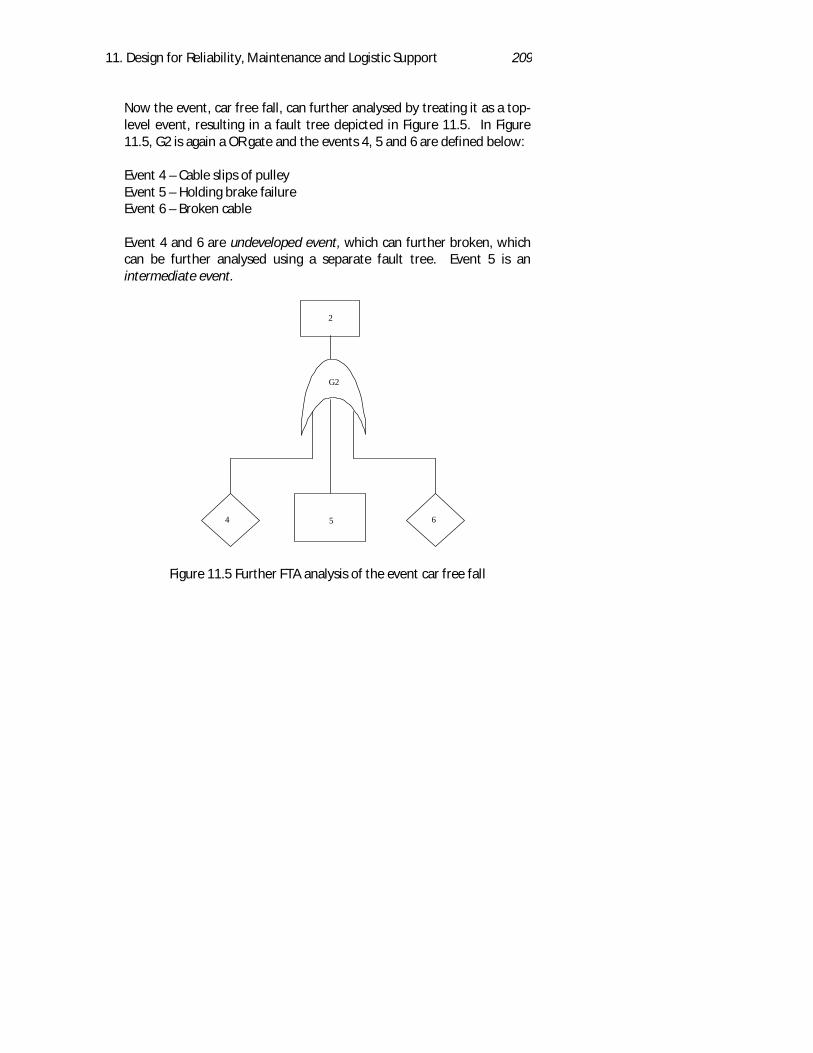
11. Design for Reliability, Maintenance and Logistic Support 209
Now the event, car free fall, can further analysed by treating it as a top-level event, resulting in a fault tree depicted in Figure 11.5. In Figure11.5, G2 is again a OR gate and the events 4, 5 and 6 are defined below:
Event 4 – Cable slips of pulleyEvent 5 – Holding brake failureEvent 6 – Broken cable
Event 4 and 6 are undeveloped event, which can further broken, whichcan be further analysed using a separate fault tree. Event 5 is anintermediate event.
Figure 11.5 Further FTA analysis of the event car free fall
2
G2
4 6 5
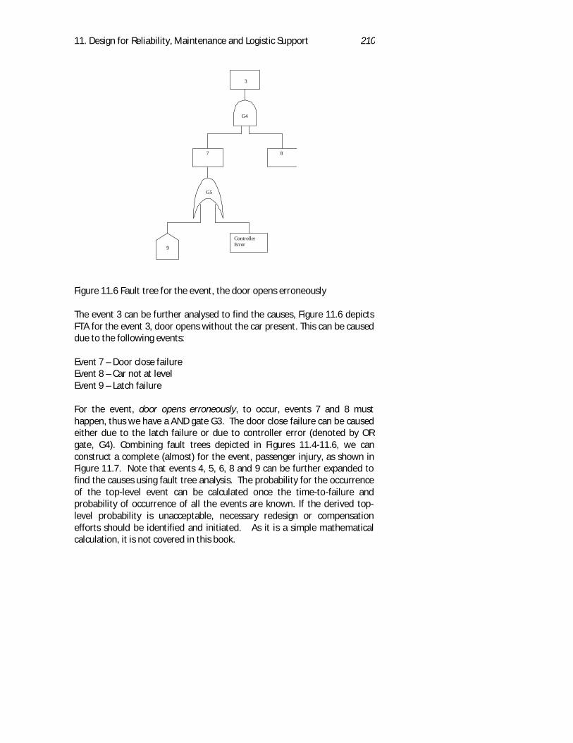
11. Design for Reliability, Maintenance and Logistic Support 210
Figure 11.6 Fault tree for the event, the door opens erroneously
The event 3 can be further analysed to find the causes, Figure 11.6 depictsFTA for the event 3, door opens without the car present. This can be causeddue to the following events:
Event 7 – Door close failureEvent 8 – Car not at levelEvent 9 – Latch failure
For the event, door opens erroneously, to occur, events 7 and 8 musthappen, thus we have a AND gate G3. The door close failure can be causedeither due to the latch failure or due to controller error (denoted by ORgate, G4). Combining fault trees depicted in Figures 11.4-11.6, we canconstruct a complete (almost) for the event, passenger injury, as shown inFigure 11.7. Note that events 4, 5, 6, 8 and 9 can be further expanded tofind the causes using fault tree analysis. The probability for the occurrenceof the top-level event can be calculated once the time-to-failure andprobability of occurrence of all the events are known. If the derived top-level probability is unacceptable, necessary redesign or compensationefforts should be identified and initiated. As it is a simple mathematicalcalculation, it is not covered in this book.
3
G4
7 8
G5
9
ControllerError
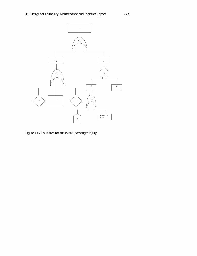
11. Design for Reliability, Maintenance and Logistic Support 211
Figure 11.7 Fault tree for the event, passenger injury
1
2 3
G1
4 6 5
G2 G3
7 8
G4
9
ControllerError
Chapter 12
Analysis of Reliability, Maintenance andSupportability Data
Often statistics are used as a drunken man uses lamp posts… for supportrather than illumination.
To predict various reliability characteristics of an item, as well as its maintainability and supportabilityfunction, it is essential that we have sufficient information on the time to failure, time to repair(maintain) and time to support characteristics of that item. In most cases these characteristics areexpressed using theoretical probability distributions. Thus, the problem which every logistician face isthe selection of the appropriate distribution function to describe the empirical data (obtained from datacapturing sources) using theoretical probability distributions. Once the distribution is identified, thenone can extract information about the type of the hazard function and other reliability characteristicssuch as mean time between failures and failure rate etc. In the case of maintenance and supportabilitydata, we would identify the maintainability and supportability function as in the case of reliability dataand then compute MTTR and MTTS.To start with we look at ways of fitting probability distributions to in-service data, that is the datarelating to the age of the components at the time they failed while they were in operation (inmaintenance and logistic support we analyse the data corresponding to the maintenance and supporttask completion times). We look at three popular tools; 1. Probability papers, 2. Linear regression, and3. Maximum likelihood estimates to identify the best distribution using which the data can be expressedand to estimate the corresponding parameters of the distribution. In the section on “censored data” werecognise that very often we do not have a complete set of failure data. We may wish to determinewhether a new version of a component is more reliable than a previous version to decide whether wehave cured the problem (of premature failures, say). Often, components will be replaced before theyhave actually failed, possibly because they have started to crack, they have been damaged or they areshowing signs of excessive wear. We may have a number of systems undergoing testing to determinewhether the product is likely to meet the various requirements but we need to go into productionbefore they have all failed. There is useful data to be gleaned from the ones that have not failed as wellas from the ones that have failed. If a component is being used in a number of different systems, it maybe reasonable to assume that the failure mechanism in each of these instances will be similar. Eventhough the way the different systems operate may be different, it is still likely that the shape of thefailure distribution will be same and that only the scale will be different.Even relatively simple systems can fail in a number of different ways and for a number of differentreasons. Suppose we wish to fasten two pieces of metal together using a nut and bolt. If we over-tighten the nut, we might strip the thread or we might shear the bolt. If we do not put the nut onsquarely, we could cross the threads and hence weaken the joint. If the two pieces of metal are beingforced apart then the stress on the nut and bolt may cause the thread to strip either inside the nut or onthe outside of the bolt or it may cause the bolt to exceed its elastic and plastic limits until it eventually
213
breaks. If the joint is subject to excessive heat this could accelerate the process. Equally, if it is in verylow temperatures then the bolt is likely to become more brittle and break under less stress than atnormal temperatures. If the diameter of the bolt is towards the lower limit of its tolerance and theinternal diameter of the nut is towards the upper limit then the amount of metal in contact may not besufficient to take the strains imposed. As the two components age, corrosion may cause the amount ofmetal in contact to be even further reduced. It may also change the tensile strength of the metals andcause premature failure.Components may therefore fail due to a number of failure modes. Each of these modes may be more orless related to the age. One would not expect corrosion to be the cause of failure during the earlystages of the component’s life, unless it was subjected to exceptionally corrosive chemicals. On theother hand, if the components have been badly made then one might expect to see them fail very soonafter the unit has been assembled.Very often, a possibly small, number of components may fail unexpectedly early. On furtherinvestigation it may be found that they were all made at the same time, from the same ingot of metal orby a particular supplier. Such a phenomenon is commonly referred to as a batching problem.Unfortunately, in practice, although it may be possible to recognise its presence, it may not always bepossible to trace its origin or, more poignantly, the other members of the same batch or, indeed, howmany there may be.
In deciding whether a new version of a component is more reliable than the old one, we need todetermine how confident we are that the two distributions are different. If they both have the same (ornearly the same) shapes then it is a relatively straightforward task to determine if their scales aredifferent. In some cases, the primary cause of failure of the origin version may have been eliminated or,at least, significantly improved but, another, hitherto rarely seen cause, may have become elevated insignificance. This new primary cause may have a distinctly different shape than the first one that oftenmakes it very difficult to decide between the two.In this chapter, we first look at the empirical approaches for finding estimates for MTTF, MTTR andMTTS as well as failure function, maintainability and supportability functions. Rest of the chapterdescribes some of the well-known methods for selection of the most relevant theoretical distributionfunctions for the random variables under consideration.
12.48. RELIABILITY, MAINTENANCE AND SUPPORTABILITY DATA
A very common problem in reliability engineering is the availability of failure data. In many cases gettingsufficient data for extracting reliable information is the most difficult task. This may be due the fact thatthere is no good procedure employed by the operator (or supplier) to collect the data or the item maybe highly reliable and the failure is very rare. However, even without any data, one should be able topredict the time-to-failure distribution if not the parameters. For example, if the failure mechanism iscorrosion, then it cannot be an exponential distribution. Similarly if the failure cause is ‘foreign objectdamage’ then the only distribution that can be used is exponential. The main problem with insufficientfailure data is getting an accurate estimate for the shape parameter. Fortunately, we don’t have suchproblems with maintenance and supportability data. These are easily available from the people whomaintain and support the item. The reliability data can be obtained from the following sources:
1. Field data and the in-service data from the operator using standard data capturing techniques.There are standard failure reporting forms for the purpose of capturing desired informationregarding the reliability of the item under consideration. Unfortunately, all these forms are
214
flawed, as they record only MTBF (or MTTR and MTTS in case of maintenance and support).Just the value of MTBF alone may not be enough for many analyses concerning reliability(similarly, in the case of maintenance (support), information on MTTR (MTTS) is not enough forcomplete analyses).
2. From life testing that involves testing a representative sample of the item under controlledconditions in a laboratory to record the required data. Sometimes, this might involve‘accelerated life testing’ (ALT) and ‘highly accelerated life testing’ (HALT) depending on theinformation required.
As mentioned earlier, in some cases it is not possible to get a complete failure data from a sample. Thisis because some of the items may not fail during the life testing (also in the in-service data). These typesof data are called ‘censored data’. If the life testing experiment is stopped before all the items havefailed, in which cases only the lower bound is known for the items that have not failed. Such type ofdata is known as ‘right censored data’. In few cases only the upper bound of the failure time may beknown, such type of data is called ‘left censored data’.
12.49. ESTIMATION OF PARAMETERS - EMPIRICAL APPROACH
The objective of empirical method is to estimate failure function, reliability function, hazard function,MTTF (or MTTR and MTTS) from the failure times (or repair and support times). Empirical approach isoften referred as non-parametric approach or distribution free approach. In the following sections wediscuss methods for estimating various performance measures used in reliability, maintenance andsupport from different types of data.
Estimation of Performance Measures - Complete Ungrouped Data
Complete ungrouped data refers to a raw data (failure, repair or support) without any censored data.That is, the failure times of the whole sample under consideration are available. For example, let t1, t2,…, tn, represents n ordered failure times such that ti ≤ ti+1. Then the possible estimate for failurefunction (cumulative failure distribution at time ti) is given by:
nitF =)(
^(12.1)
A total of i units fail by time t out of the total n in the sample. This will make F(tn) = n /n = 1. That is,there is a zero probability for any item to survive beyond time tn. This is very unlikely, as the times aredrawn from a sample and it is extremely unlikely that any sample would include the longest survivaltime. Thus the equation (12.1) underestimates the component survival function. A number ofmathematicians have tried to find a suitable alternative method of estimating the cumulative failureprobability. These range from using n+1 in the denominator to using -0.5 in the numerator and +0.5 inthe denominator. The one that gives the best approximation is based on median rank. Bernard'sapproximation to the median rank approach for cumulative failure probability is given by
4.03.0)(
^
+−
=nitF i (12.2)
215
Throughout this chapter we use the above approximation to estimate the cumulative failure distributionor failure function. From equation (12.2), the estimate for reliability function can be obtained as
4.07.0
4.03.01)(1)(
^^
++−
=+−
−=−=n
innitFtR ii (12.3)
The estimate for the failure density function f(t) can be obtained using
11
1
^^^
,)()(
)( ++
+ ≤≤−−
= iiii
ii ttttt
tFtFtf (12.4)
Estimate for the hazard function can be obtained by using the relation between the reliability functionR(t) and the failure density function f(t). Therefore,
1
^^^for)()()( +<<= ii ttttRtfth (12.5)
An estimate for the mean time to failure (or mean time to repair or mean time to support) can bedirectly obtained from the sample mean. That is,
∑=
=n
i
intMTTF
1
^(12.6)
Estimate for the variance of the failure distribution can be obtained from the sample variance, that is
∑= −
−=
n
i
i
nMTTFt
s1
2^
2
1)(
(12.7)
Estimate for MTTR (MTTS) and Variance of time to repair distribution (time to support distribution) canbe obtained by replacing failure times by repair times (support times) in equation (12.6) and (12.7)respectively.
Confidence Interval
It is always of the interest to know the range in which the measures such as MTTF, MTTR and MTTSmight lie with certain confidence. The resulting interval is called a confidence interval and theprobability that it contains the estimated parameter is called its confidence level or confidencecoefficient. For example, if a confidence interval has a confidence coefficient equal to 0.95, we call it a95% confidence interval.
To derive a (1-α) 100% confidence interval for a large sample we use the following expression:
)(2/
^
nzMTTF σ
α± (12.8)
216
Where zα/2 is the z value (standard normal statistic) that locates an area of α/2 to its right and can befound from the normal table. σ is the standard deviation of the population from which the populationwas selected and n is the sample size. The above formula is valid whenever the sample size n is greaterthan or equal to 30. The 90%, 95% and 99% confidence interval for MTTF with sample size n ≥ 30 aregiven below:
×±
nMTTF σ645.1confidence%90
^(12.9)
×±
nMTTF σ96.1confidence%95
^(12.10)
×±
nMTTF σ58..2confidence%99
^(12.11)
When the number of data is small (that is when n is less than 30), the confidence interval is based on tdistribution. We use the following expression to calculate (1-α)100% confidence interval.
±
nstMTTF 2/
^
α (12.12)
where tα/2 is based on (n-1) degrees of freedom and can be obtained from t distribution table (referappendix).
Example 12.1
Time to failure data for 20 car gearboxes of the model M2000 is listed in Table 12.1. Find:
1. Estimate of failure function and reliability function.2. Plot failure function and the reliability function.3. Estimate of MTTF and 95% confidence interval.
Table 12.1. Failure data of gearboxes in miles
1022 1617 2513 3265 84459007 10505 11490 13086 1416214363 15456 16736 16936 1801219030 19365 19596 19822 20079
SOLUTION:
The failure function and reliability function can be estimated using equations 12.2 and 12.3. Table 12.2shows the estimated values of failure function and reliability function.
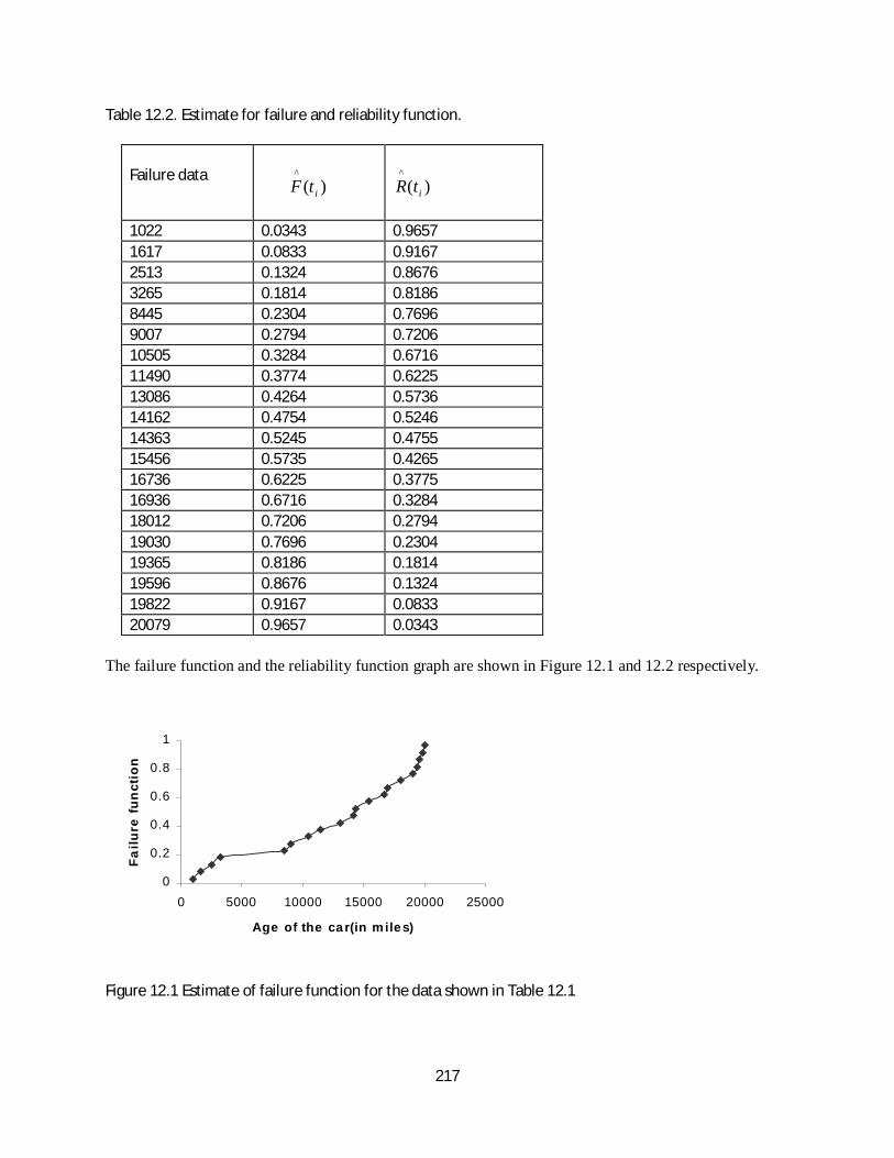
217
Table 12.2. Estimate for failure and reliability function.
Failure data)(
^
itF )(^
itR
1022 0.0343 0.96571617 0.0833 0.91672513 0.1324 0.86763265 0.1814 0.81868445 0.2304 0.76969007 0.2794 0.720610505 0.3284 0.671611490 0.3774 0.622513086 0.4264 0.573614162 0.4754 0.524614363 0.5245 0.475515456 0.5735 0.426516736 0.6225 0.377516936 0.6716 0.328418012 0.7206 0.279419030 0.7696 0.230419365 0.8186 0.181419596 0.8676 0.132419822 0.9167 0.083320079 0.9657 0.0343
The failure function and the reliability function graph are shown in Figure 12.1 and 12.2 respectively.
Figure 12.1 Estimate of failure function for the data shown in Table 12.1
0
0.2
0.4
0.6
0.8
1
0 5000 10000 15000 20000 25000
Age of the car(in miles)
Failu
re f
unct
ion
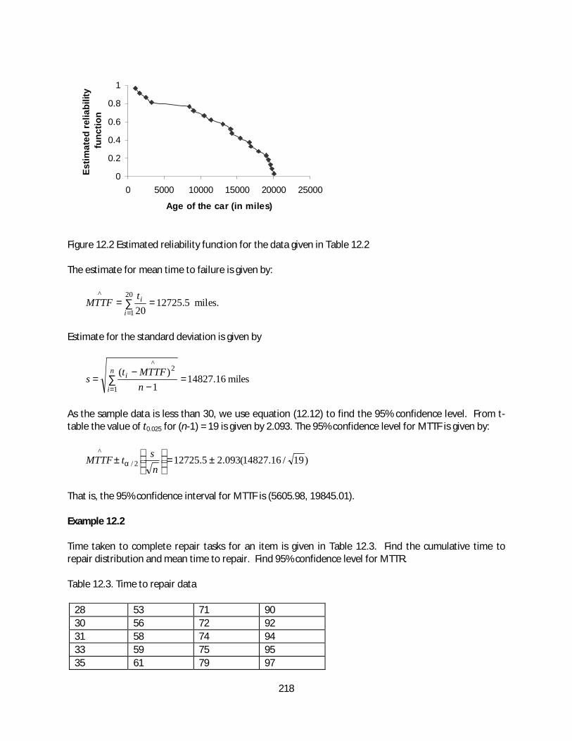
218
Figure 12.2 Estimated reliability function for the data given in Table 12.2
The estimate for mean time to failure is given by:
∑=
==20
1
^5.12725
20i
itMTTF miles.
Estimate for the standard deviation is given by
miles16.148271
)(1
2^
=−
−= ∑
=
n
i
i
nMTTFt
s
As the sample data is less than 30, we use equation (12.12) to find the 95% confidence level. From t-table the value of t0.025 for (n-1) = 19 is given by 2.093. The 95% confidence level for MTTF is given by:
)19/16.14827(093.25.127252/
^±=
±
nstMTTF α
That is, the 95% confidence interval for MTTF is (5605.98, 19845.01).
Example 12.2
Time taken to complete repair tasks for an item is given in Table 12.3. Find the cumulative time torepair distribution and mean time to repair. Find 95% confidence level for MTTR.
Table 12.3. Time to repair data
28 53 71 9030 56 72 9231 58 74 9433 59 75 9535 61 79 97
0
0.2
0.4
0.6
0.8
1
0 5000 10000 15000 20000 25000
Age of the car (in miles)
Estim
ated
relia
bilit
yfu
nctio
n
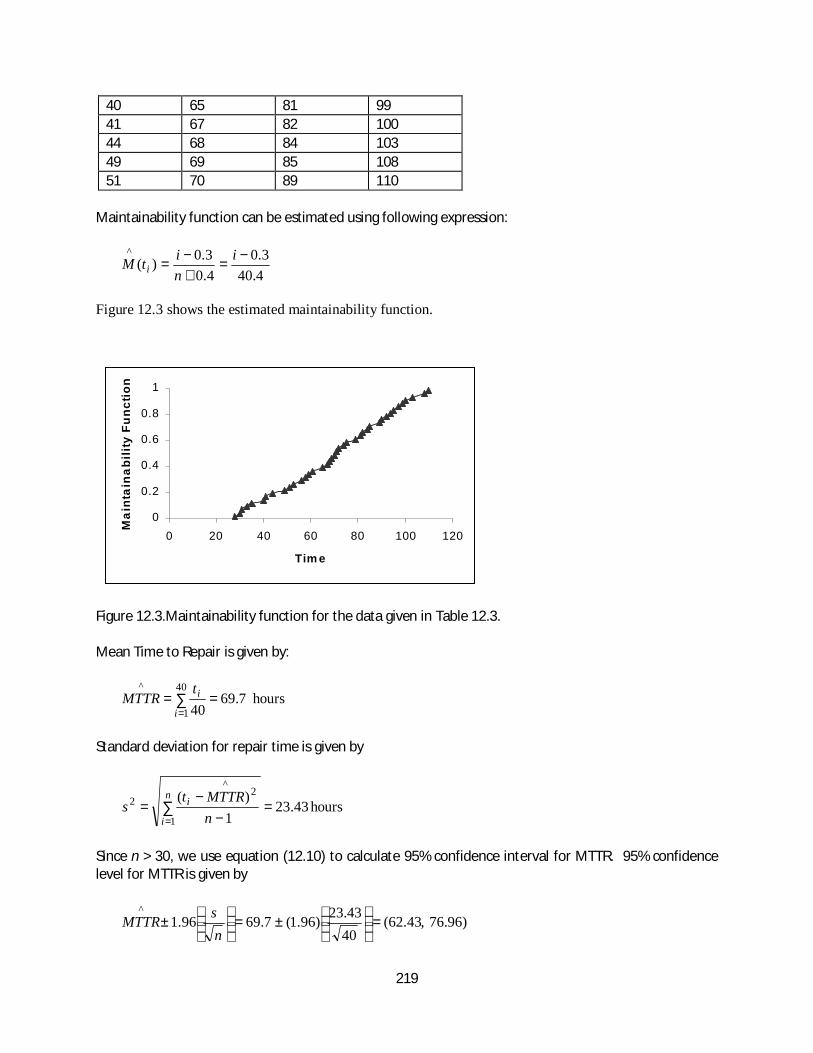
219
40 65 81 9941 67 82 10044 68 84 10349 69 85 10851 70 89 110
Maintainability function can be estimated using following expression:
4.403.0
4.03.0)(
^ −=
+−
=i
nitM i
Figure 12.3 shows the estimated maintainability function.
Figure 12.3.Maintainability function for the data given in Table 12.3.
Mean Time to Repair is given by:
hours7.6940
40
1
^== ∑
=i
itMTTR
Standard deviation for repair time is given by
hours23.431
)(1
2^
2 =−
−= ∑
=
n
i
i
nMTTRt
s
Since n > 30, we use equation (12.10) to calculate 95% confidence interval for MTTR. 95% confidencelevel for MTTR is given by
)96.76,43.62(4043.23)96.1(7.6996.1
^=
±=
±
nsMTTR
0
0.2
0.4
0.6
0.8
1
0 20 40 60 80 100 120
Tim e
Mai
ntai
nab
ility
Fu
ncti
on
220
Analysis of Grouped Data
Often failure data is placed into time intervals when the sample size is large. The failure data areclassified into several intervals. The number of intervals, NI, depends on the total number of data n.Following equation can be used as guidance for determining the suitable number of intervals:
)(log3.31 10 nNI ×+= (12.13)
NI denotes that the value is rounded down to the nearest integer.
The length of each interval, LI, is calculated using:
( ) NI
xxLI minmax −
= (12.14)
where xmax is the maximum recorded failure time and xmin is the minimum recorded failure time. Thelower and upper bound of each interval is calculated as follows:
LIixX
LIixX
i
i
×+=
×−+=
minmax,
minmin, )1(
Xmin,i is the lower bound of the ith interval and Xmax,i is the upper bound value of the ith interval. Let n1,n2 , … nn be the number of items that fail in the interval i. Then the estimate for cumulative failuredistribution is given by
4.0
3.0)( 1
max,
^
+
−=
∑=
n
nXF
i
kk
i (12.15)
Estimate for the reliability function R(t) is given by:
4.0
7.0)(1)( 1
max,
^
max,
^
+
+=−=
∑+=
n
nXFXR
n
iki
ii (12.16)
Estimate for the failure density is given by:
For Xmax,i+1 < t < Xmax,i
)()4.0()()(
)(max,1max,
1
max,1max,
max,1max,
^^
ii
i
ii
ii
XXnn
XXXFXF
tf−×+
=−
−=
+
+
+
+
The MTTF is estimated using the expression:
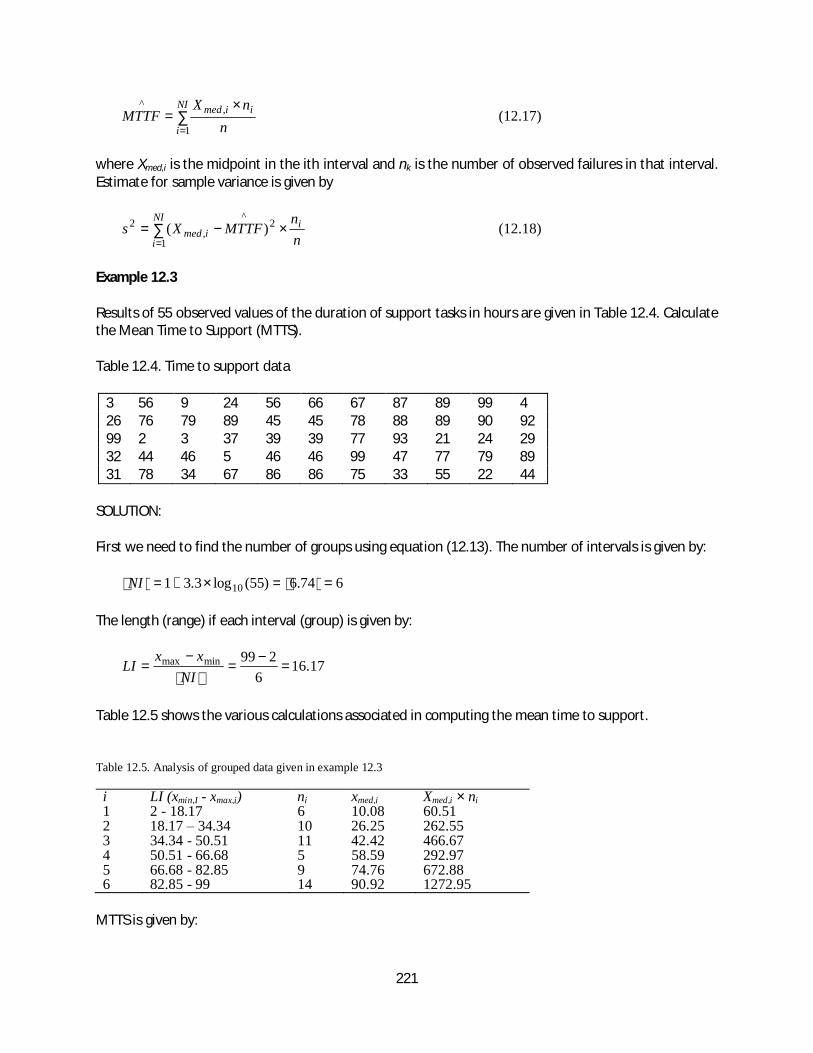
221
∑=
×=
NI
i
iimed
nnX
MTTF1
,^(12.17)
where Xmed,i is the midpoint in the ith interval and nk is the number of observed failures in that interval.Estimate for sample variance is given by
∑=
×−=NI
i
iimed n
nMTTFXs
1
2^
,2 )( (12.18)
Example 12.3
Results of 55 observed values of the duration of support tasks in hours are given in Table 12.4. Calculatethe Mean Time to Support (MTTS).
Table 12.4. Time to support data
3 56 9 24 56 66 67 87 89 99 426 76 79 89 45 45 78 88 89 90 9299 2 3 37 39 39 77 93 21 24 2932 44 46 5 46 46 99 47 77 79 8931 78 34 67 86 86 75 33 55 22 44
SOLUTION:
First we need to find the number of groups using equation (12.13). The number of intervals is given by:
674.6)55(log3.31 10 ==×+=NI
The length (range) if each interval (group) is given by:
17.16
6299minmax =
−=
−=
NIxx
LI
Table 12.5 shows the various calculations associated in computing the mean time to support.
Table 12.5. Analysis of grouped data given in example 12.3
i LI (xmin,I - xmax,i) ni xmed,i Xmed,i × ni1 2 - 18.17 6 10.08 60.512 18.17 34.34 10 26.25 262.553 34.34 - 50.51 11 42.42 466.674 50.51 - 66.68 5 58.59 292.975 66.68 - 82.85 9 74.76 672.886 82.85 - 99 14 90.92 1272.95
MTTS is given by:
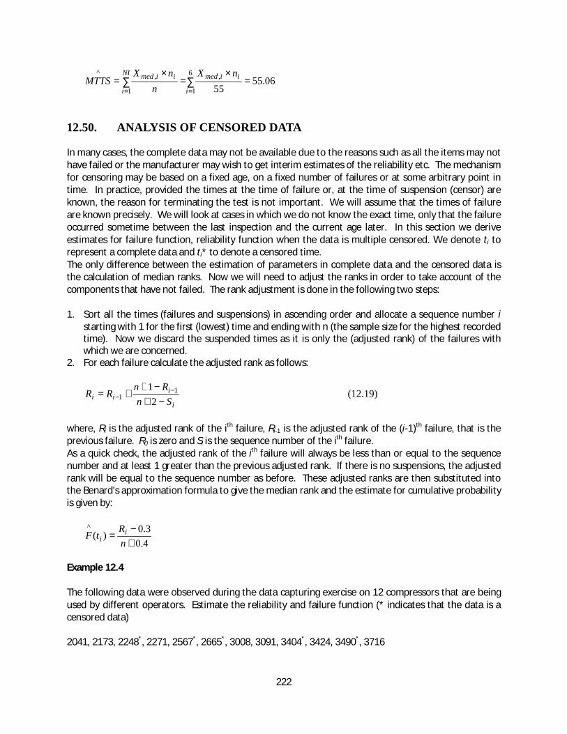
222
∑∑==
=×
=×
=6
1
,
1
,^06.55
55i
iimedNI
i
iimed nXn
nXMTTS
12.50. ANALYSIS OF CENSORED DATA
In many cases, the complete data may not be available due to the reasons such as all the items may nothave failed or the manufacturer may wish to get interim estimates of the reliability etc. The mechanismfor censoring may be based on a fixed age, on a fixed number of failures or at some arbitrary point intime. In practice, provided the times at the time of failure or, at the time of suspension (censor) areknown, the reason for terminating the test is not important. We will assume that the times of failureare known precisely. We will look at cases in which we do not know the exact time, only that the failureoccurred sometime between the last inspection and the current age later. In this section we deriveestimates for failure function, reliability function when the data is multiple censored. We denote ti torepresent a complete data and ti* to denote a censored time.The only difference between the estimation of parameters in complete data and the censored data isthe calculation of median ranks. Now we will need to adjust the ranks in order to take account of thecomponents that have not failed. The rank adjustment is done in the following two steps:
1. Sort all the times (failures and suspensions) in ascending order and allocate a sequence number istarting with 1 for the first (lowest) time and ending with n (the sample size for the highest recordedtime). Now we discard the suspended times as it is only the (adjusted rank) of the failures withwhich we are concerned.
2. For each failure calculate the adjusted rank as follows:
i
iii Sn
RnRR
−+−+
+= −− 2
1 11 (12.19)
where, Ri is the adjusted rank of the ith failure, Ri-1 is the adjusted rank of the (i-1)th failure, that is theprevious failure. R0 is zero and Si is the sequence number of the ith failure.As a quick check, the adjusted rank of the ith failure will always be less than or equal to the sequencenumber and at least 1 greater than the previous adjusted rank. If there is no suspensions, the adjustedrank will be equal to the sequence number as before. These adjusted ranks are then substituted intothe Benard's approximation formula to give the median rank and the estimate for cumulative probabilityis given by:
4.03.0)(
^
+−
=nRtF i
i
Example 12.4
The following data were observed during the data capturing exercise on 12 compressors that are beingused by different operators. Estimate the reliability and failure function (* indicates that the data is acensored data)
2041, 2173, 2248*, 2271, 2567*, 2665*, 3008, 3091, 3404*, 3424, 3490*, 3716
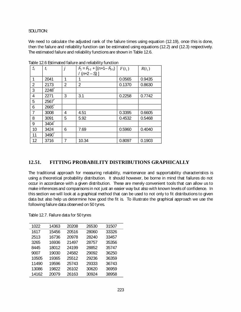
223
SOLUTION:
We need to calculate the adjusted rank of the failure times using equation (12.19), once this is done,then the failure and reliability function can be estimated using equations (12.2) and (12.3) respectively.The estimated failure and reliability functions are shown in Table 12.6.
Table 12.6 Estimated failure and reliability functionSi ti j Rj = Rj-1 + [(n+1– Rj-1)
/ (n+2 – Si) ])( itF )( itR
1 2041 1 1 0.0565 0.94352 2173 2 2 0.1370 0.86303 2248*
4 2271 3 3.1 0.2258 0.77425 2567*
6 2665*
7 3008 4 4.51 0.3395 0.66058 3091 5 5.92 0.4532 0.54689 3404*
10 3424 6 7.69 0.5960 0.404011 3490*
12 3716 7 10.34 0.8097 0.1903
12.51. FITTING PROBABILITY DISTRIBUTIONS GRAPHICALLY
The traditional approach for measuring reliability, maintenance and supportability characteristics isusing a theoretical probability distribution. It should however, be borne in mind that failures do notoccur in accordance with a given distribution. These are merely convenient tools that can allow us tomake inferences and comparisons in not just an easier way but also with known levels of confidence. Inthis section we will look at a graphical method that can be used to not only to fit distributions to givendata but also help us determine how good the fit is. To illustrate the graphical approach we use thefollowing failure data observed on 50 tyres.
Table 12.7. Failure data for 50 tyres
1022 14363 20208 26530 315071617 15456 20516 28060 333262513 16736 20978 28240 334573265 16936 21497 28757 353568445 18012 24199 28852 357479007 19030 24582 29092 3625010505 19365 25512 29236 3635911490 19596 25743 29333 3674313086 19822 26102 30620 3695914162 20079 26163 30924 38958
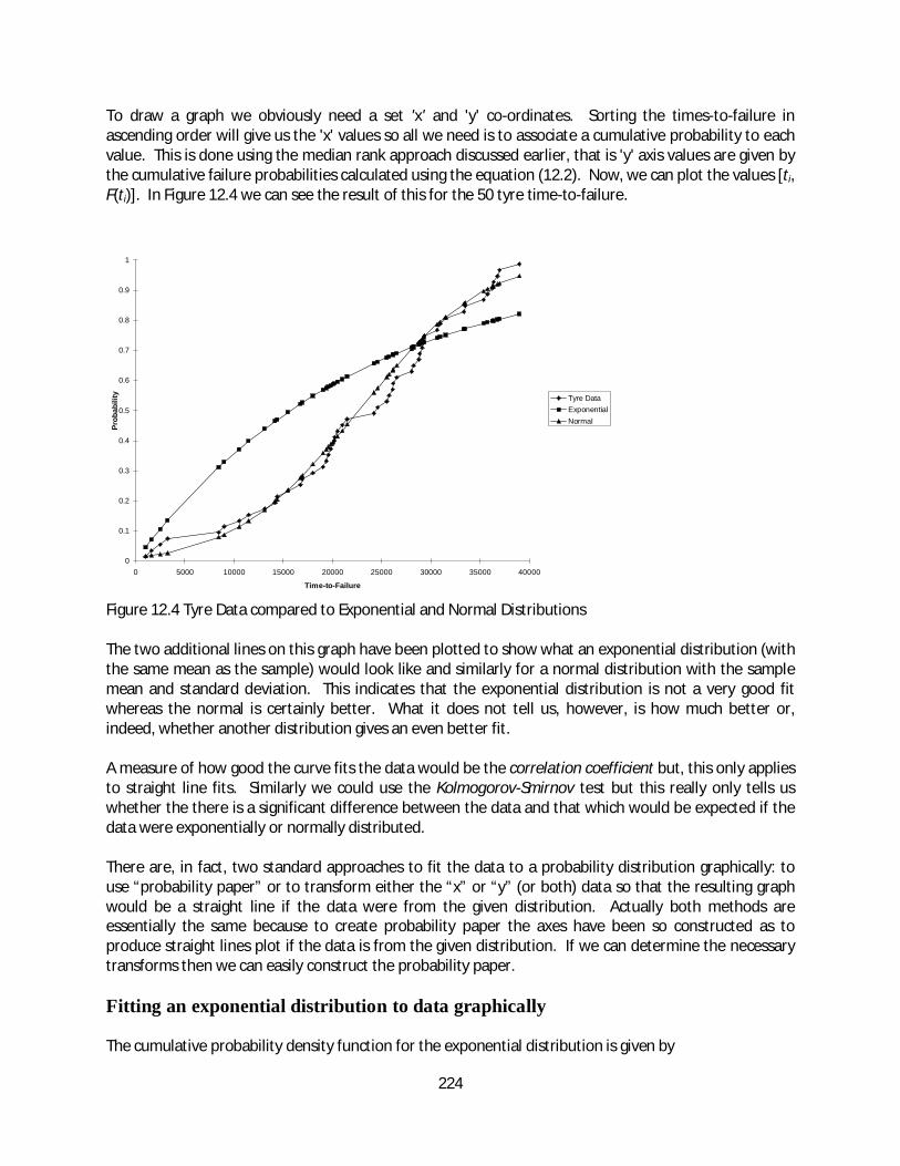
224
To draw a graph we obviously need a set 'x' and 'y' co-ordinates. Sorting the times-to-failure inascending order will give us the 'x' values so all we need is to associate a cumulative probability to eachvalue. This is done using the median rank approach discussed earlier, that is 'y' axis values are given bythe cumulative failure probabilities calculated using the equation (12.2). Now, we can plot the values [ti,F(ti)]. In Figure 12.4 we can see the result of this for the 50 tyre time-to-failure.
Figure 12.4 Tyre Data compared to Exponential and Normal Distributions
The two additional lines on this graph have been plotted to show what an exponential distribution (withthe same mean as the sample) would look like and similarly for a normal distribution with the samplemean and standard deviation. This indicates that the exponential distribution is not a very good fitwhereas the normal is certainly better. What it does not tell us, however, is how much better or,indeed, whether another distribution gives an even better fit.
A measure of how good the curve fits the data would be the correlation coefficient but, this only appliesto straight line fits. Similarly we could use the Kolmogorov-Smirnov test but this really only tells uswhether the there is a significant difference between the data and that which would be expected if thedata were exponentially or normally distributed.
There are, in fact, two standard approaches to fit the data to a probability distribution graphically: touse “probability paper” or to transform either the “x” or “y” (or both) data so that the resulting graphwould be a straight line if the data were from the given distribution. Actually both methods areessentially the same because to create probability paper the axes have been so constructed as toproduce straight lines plot if the data is from the given distribution. If we can determine the necessarytransforms then we can easily construct the probability paper.
Fitting an exponential distribution to data graphically
The cumulative probability density function for the exponential distribution is given by
0
0.1
0.2
0.3
0.4
0.5
0.6
0.7
0.8
0.9
1
0 5000 10000 15000 20000 25000 30000 35000 40000
Time-to-Failure
Prob
abili
ty Tyre DataExponentialNormal
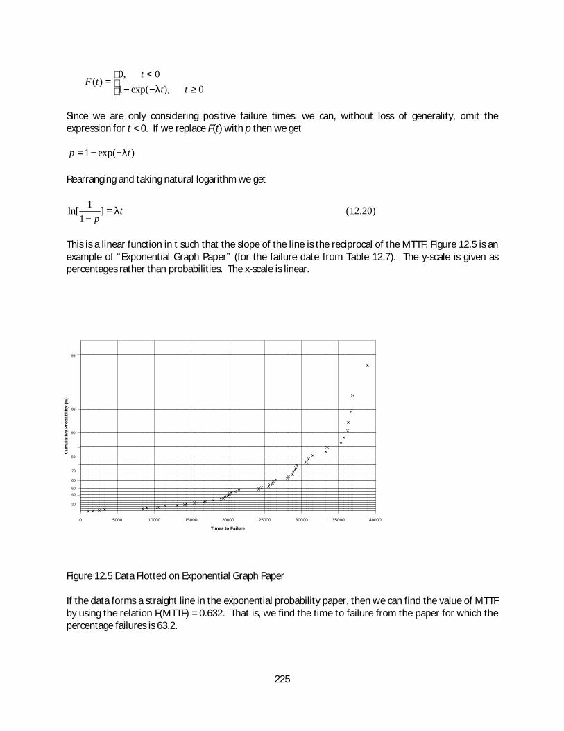
225
≥−−<
=0),exp(1
0,0)(
ttt
tFλ
Since we are only considering positive failure times, we can, without loss of generality, omit theexpression for t < 0. If we replace F(t) with p then we get
)exp(1 tp λ−−=
Rearranging and taking natural logarithm we get
tp
λ=−
]1
1ln[ (12.20)
This is a linear function in t such that the slope of the line is the reciprocal of the MTTF. Figure 12.5 is anexample of “Exponential Graph Paper” (for the failure date from Table 12.7). The y-scale is given aspercentages rather than probabilities. The x-scale is linear.
Figure 12.5 Data Plotted on Exponential Graph Paper
If the data forms a straight line in the exponential probability paper, then we can find the value of MTTFby using the relation F(MTTF) = 0.632. That is, we find the time to failure from the paper for which thepercentage failures is 63.2.
0 5000 10000 15000 20000 25000 30000 35000 40000
Times to Failure
Cum
ulat
ive
Prob
abili
ty (%
)
99
95
90
80
70
60
5040
20
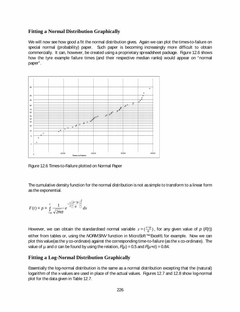
226
Fitting a Normal Distribution Graphically
We will now see how good a fit the normal distribution gives. Again we can plot the times-to-failure onspecial normal (probability) paper. Such paper is becoming increasingly more difficult to obtaincommercially. It can, however, be created using a proprietary spreadsheet package. Figure 12.6 showshow the tyre example failure times (and their respective median ranks) would appear on “normalpaper”.
Figure 12.6 Times-to-Failure plotted on Normal Paper
The cumulative density function for the normal distribution is not as simple to transform to a linear formas the exponential.
dxeptFt
x
∫∞−
−
−==
2
21
21)( σ
µ
σπ
However, we can obtain the standardised normal variable )( σµ−= xz , for any given value of p (F(t))
either from tables or, using the NORMSINV function in MicroSoft™ Excel®, for example. Now we canplot this value(as the y co-ordinate) against the corresponding time-to-failure (as the x co-ordinate). Thevalue of µ and σ can be found by using the relation, F(µ) = 0.5 and F(µ+σ) = 0.84.
Fitting a Log-Normal Distribution Graphically
Essentially the log-normal distribution is the same as a normal distribution excepting that the (natural)logarithm of the x-values are used in place of the actual values. Figures 12.7 and 12.8 show log-normalplot for the data given in Table 12.7.
Times to Failure0 10000 20000 30000 40000
99
95
90
80
7060
504030
20
10
5
1
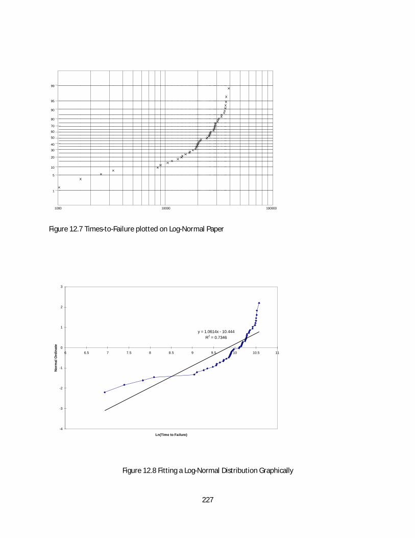
227
Figure 12.7 Times-to-Failure plotted on Log-Normal Paper
Figure 12.8 Fitting a Log-Normal Distribution Graphically
1000 10000 100000
99
95
90
80
70
60
50
40
30
20
10
5
1
y = 1.0614x - 10.444R2 = 0.7346
-4
-3
-2
-1
0
1
2
3
6 6.5 7 7.5 8 8.5 9 9.5 10 10.5 11
Ln(Time to Failure)
Nor
mal
Ord
inat
e
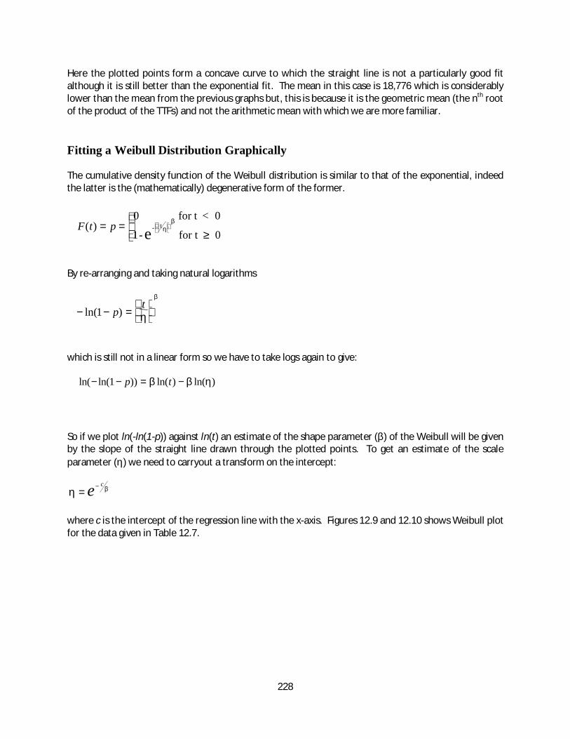
228
Here the plotted points form a concave curve to which the straight line is not a particularly good fitalthough it is still better than the exponential fit. The mean in this case is 18,776 which is considerablylower than the mean from the previous graphs but, this is because it is the geometric mean (the nth rootof the product of the TTFs) and not the arithmetic mean with which we are more familiar.
Fitting a Weibull Distribution Graphically
The cumulative density function of the Weibull distribution is similar to that of the exponential, indeedthe latter is the (mathematically) degenerative form of the former.
By re-arranging and taking natural logarithms
which is still not in a linear form so we have to take logs again to give:
So if we plot ln(-ln(1-p)) against ln(t) an estimate of the shape parameter (β) of the Weibull will be givenby the slope of the straight line drawn through the plotted points. To get an estimate of the scaleparameter (η) we need to carryout a transform on the intercept:
where c is the intercept of the regression line with the x-axis. Figures 12.9 and 12.10 shows Weibull plotfor the data given in Table 12.7.
F t p( ) = =≥
0 for t < 0
1- for t 0e - t ηβ
− − =
ln( )1 ptη
β
ln( ln( )) ln( ) ln( )− − = −1 p tβ β η
η β=−e c
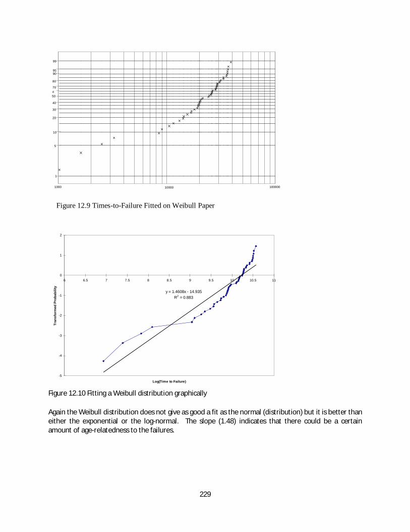
229
Figure 12.9 Times-to-Failure Fitted on Weibull Paper
Figure 12.10 Fitting a Weibull distribution graphically
Again the Weibull distribution does not give as good a fit as the normal (distribution) but it is better thaneither the exponential or the log-normal. The slope (1.48) indicates that there could be a certainamount of age-relatedness to the failures.
99
9590
80
70650
40
30
20
10
5
1
1000 10000 100000
y = 1.4608x - 14.935R2 = 0.883
-5
-4
-3
-2
-1
0
1
2
6 6.5 7 7.5 8 8.5 9 9.5 10 10.5 11
Log(Time to Failure)
Tran
sfor
med
Pro
babi
lity
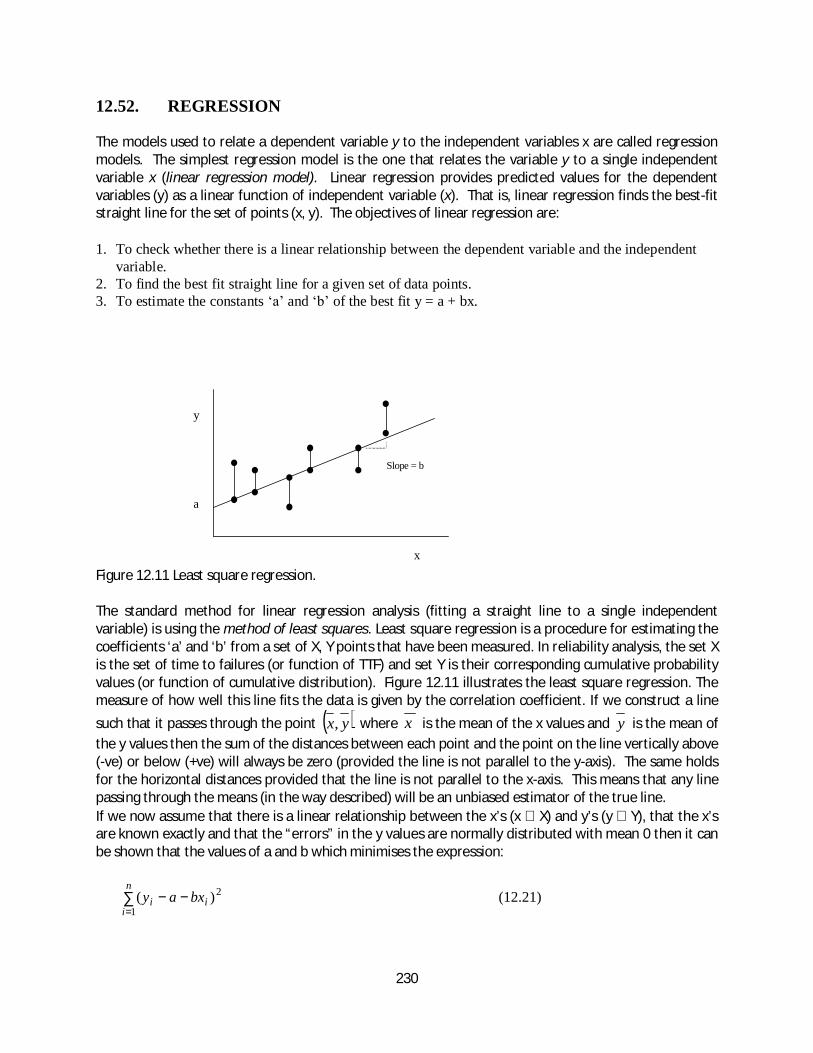
230
12.52. REGRESSION
The models used to relate a dependent variable y to the independent variables x are called regressionmodels. The simplest regression model is the one that relates the variable y to a single independentvariable x (linear regression model). Linear regression provides predicted values for the dependentvariables (y) as a linear function of independent variable (x). That is, linear regression finds the best-fitstraight line for the set of points (x, y). The objectives of linear regression are:
1. To check whether there is a linear relationship between the dependent variable and the independentvariable.
2. To find the best fit straight line for a given set of data points.3. To estimate the constants and of the best fit y = a + bx.
Figure 12.11 Least square regression.
The standard method for linear regression analysis (fitting a straight line to a single independentvariable) is using the method of least squares. Least square regression is a procedure for estimating thecoefficients ‘a’ and ‘b’ from a set of X, Y points that have been measured. In reliability analysis, the set Xis the set of time to failures (or function of TTF) and set Y is their corresponding cumulative probabilityvalues (or function of cumulative distribution). Figure 12.11 illustrates the least square regression. Themeasure of how well this line fits the data is given by the correlation coefficient. If we construct a line
such that it passes through the point ( )yx, where x is the mean of the x values and y is the mean ofthe y values then the sum of the distances between each point and the point on the line vertically above(-ve) or below (+ve) will always be zero (provided the line is not parallel to the y-axis). The same holdsfor the horizontal distances provided that the line is not parallel to the x-axis. This means that any linepassing through the means (in the way described) will be an unbiased estimator of the true line.If we now assume that there is a linear relationship between the x’s (x ∈ X) and y’s (y ∈ Y), that the x’sare known exactly and that the “errors” in the y values are normally distributed with mean 0 then it canbe shown that the values of a and b which minimises the expression:
∑=
−−n
iii bxay
1
2)( (12.21)
y
a
x
Slope = b
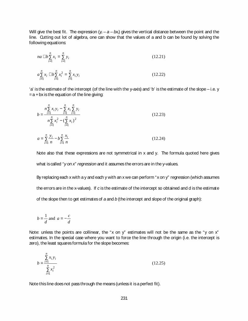
231
Will give the best fit. The expression (yi – a – bxi) gives the vertical distance between the point and theline. Cutting out lot of algebra, one can show that the values of a and b can be found by solving thefollowing equations:
∑∑==
=+n
ii
n
ii yxbna
11(12.21)
∑∑∑===
=+n
iii
n
ii
n
ii yxxbxa
11
2
1(12.22)
‘a’ is the estimate of the intercept (of the line with the y-axis) and ‘b’ is the estimate of the slope – i.e. y= a + bx is the equation of the line giving:
2
11
2
111
)(∑∑
∑∑∑
==
===
−
−= n
ii
n
ii
n
ii
n
ii
n
iii
xxn
yxyxnb (12.23)
∑∑==
−=n
i
in
i
inx
bny
a11
(12.24)
Note also that these expressions are not symmetrical in x and y. The formula quoted here gives
what is called “y on x” regression and it assumes the errors are in the y-values.
By replacing each x with a y and each y with an x we can perform “x on y” regression (which assumes
the errors are in the x-values). If c is the estimate of the intercept so obtained and d is the estimate
of the slope then to get estimates of a and b (the intercept and slope of the original graph):
db 1
= anddca −=
Note: unless the points are collinear, the “x on y” estimates will not be the same as the “y on x”estimates. In the special case where you want to force the line through the origin (i.e. the intercept iszero), the least squares formula for the slope becomes:
∑
∑
=
== n
ii
n
iii
x
yxb
1
2
1 (12.25)
Note this line does not pass through the means (unless it is a perfect fit).
232
Correlation Co-efficient
A measure of the dependence between two variables is given by the correlation coefficient. Thecorrelation coefficient, r is given by:
2
11
22
11
2
111
)()( ∑∑∑∑
∑∑∑
====
===
−×−
−=
n
ii
n
ii
n
ii
n
ii
n
ii
n
ii
n
iii
yynxxn
yxyxnr (12.26)
The correlation coefficient always lies between –1 and +1. A value of +1 or –1 means that x and y areexactly linearly related. In the former case y increases as x increases but for r = -1, y decreases as xincreases. Note that if x and y are independent then r = 0, but r = 0 does not mean that x and y areindependent. The best fit distribution is the one with maximum r value (close to one). To find the bestfit, regression analysis is carried out on the popular distribution such as exponential, Weibull, normaland log-normal. The one with highest correlation coefficient is selected as the best. The coordinates (x,y) and the corresponding parameters for different distributions are listed given in the following sections.
Linear Regression for Exponential Distribution
To fit a data to an exponential distribution, we transform the co-ordinates (ti, F(ti)) such a way that,when plotted, it gives a straight line. Here ti is the observed failure times and F(ti) is the estimatedcumulative distribution function. The cumulative distribution of exponential distribution is given by:
)exp(1)( ttF λ−−=
that is,
ttF
λ=−
])(1
1ln[ (12.27)
Equation (12.27) is a linear function. Thus, for an exponential distribution, the plot of ( ])(1
1ln[,tF
t−
)
provides a straight line. Thus, if t1, t2, , tn are the observed failure times, then to fit this data into anexponential distribution, we set:
ii tx = (12.28)
])(1
1ln[i
i tFy
−= (12.29)
Substituting (xi , yi) in equation (12.23) we get:
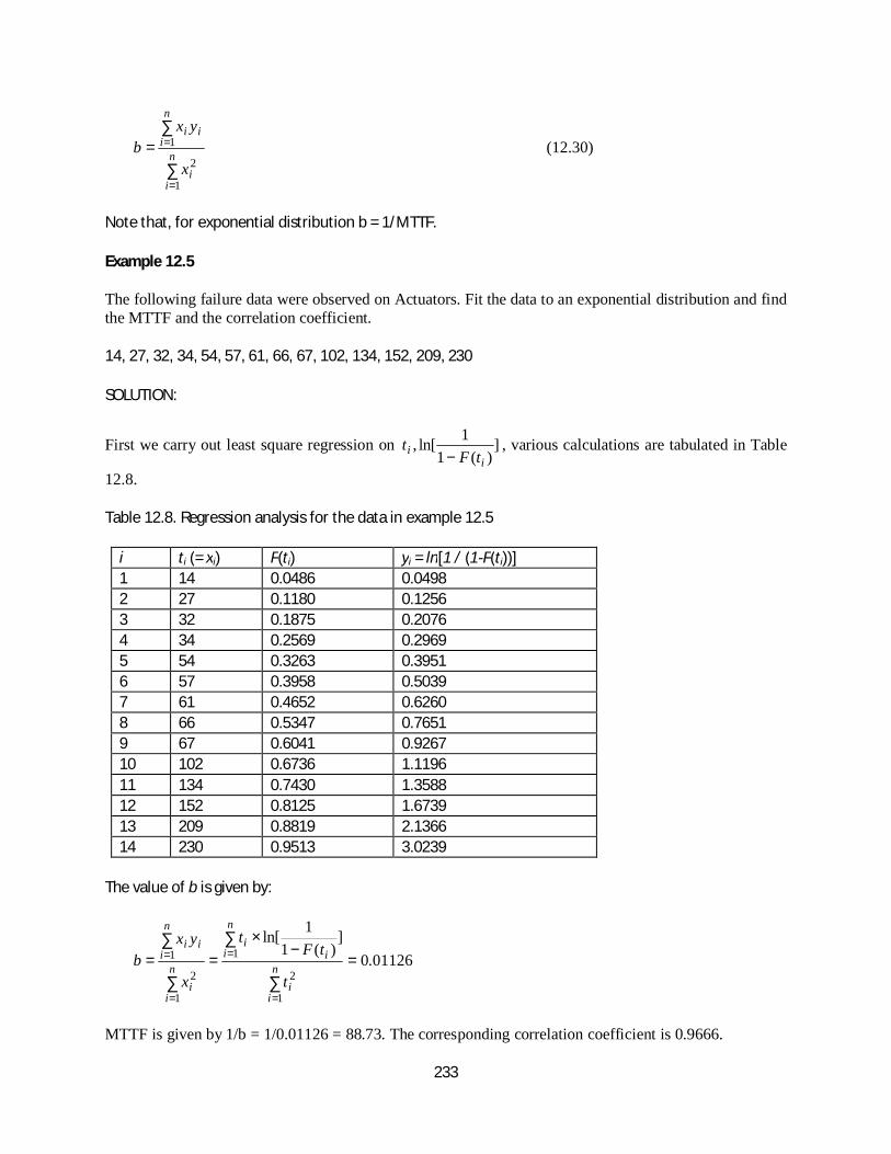
233
∑
∑
=
== n
ii
n
iii
x
yxb
1
2
1 (12.30)
Note that, for exponential distribution b = 1/MTTF.
Example 12.5
The following failure data were observed on Actuators. Fit the data to an exponential distribution and findthe MTTF and the correlation coefficient.
14, 27, 32, 34, 54, 57, 61, 66, 67, 102, 134, 152, 209, 230
SOLUTION:
First we carry out least square regression on ])(1
1ln[,i
i tFt
−, various calculations are tabulated in Table
12.8.
Table 12.8. Regression analysis for the data in example 12.5
i ti (= xi) F(ti) yi = ln[1 / (1-F(ti))]1 14 0.0486 0.04982 27 0.1180 0.12563 32 0.1875 0.20764 34 0.2569 0.29695 54 0.3263 0.39516 57 0.3958 0.50397 61 0.4652 0.62608 66 0.5347 0.76519 67 0.6041 0.926710 102 0.6736 1.119611 134 0.7430 1.358812 152 0.8125 1.673913 209 0.8819 2.136614 230 0.9513 3.0239
The value of b is given by:
01126.0]
)(11ln[
1
2
1
1
2
1 =−
×==
∑
∑
∑
∑
=
=
=
=n
ii
n
i ii
n
ii
n
iii
t
tFt
x
yxb
MTTF is given by 1/b = 1/0.01126 = 88.73. The corresponding correlation coefficient is 0.9666.
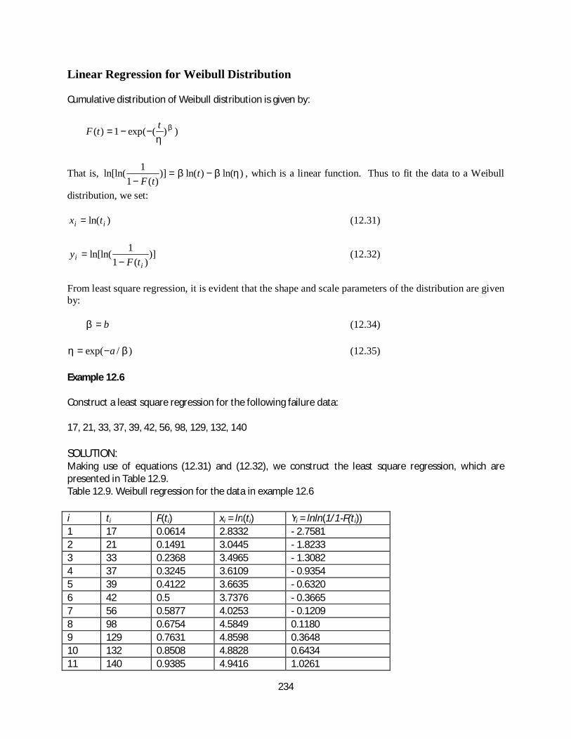
234
Linear Regression for Weibull Distribution
Cumulative distribution of Weibull distribution is given by:
))(exp(1)( β
ηttF −−=
That is, )ln()ln()])(1
1ln[ln( ηββ −=−
ttF
, which is a linear function. Thus to fit the data to a Weibull
distribution, we set:
)ln( ii tx = (12.31)
)])(1
1ln[ln(i
i tFy
−= (12.32)
From least square regression, it is evident that the shape and scale parameters of the distribution are givenby:
b=β (12.34)
)/exp( βη a−= (12.35)
Example 12.6
Construct a least square regression for the following failure data:
17, 21, 33, 37, 39, 42, 56, 98, 129, 132, 140
SOLUTION:Making use of equations (12.31) and (12.32), we construct the least square regression, which arepresented in Table 12.9.Table 12.9. Weibull regression for the data in example 12.6
i ti F(ti) xi = ln(ti) Yi = lnln(1/1-F(ti))1 17 0.0614 2.8332 - 2.75812 21 0.1491 3.0445 - 1.82333 33 0.2368 3.4965 - 1.30824 37 0.3245 3.6109 - 0.93545 39 0.4122 3.6635 - 0.63206 42 0.5 3.7376 - 0.36657 56 0.5877 4.0253 - 0.12098 98 0.6754 4.5849 0.11809 129 0.7631 4.8598 0.364810 132 0.8508 4.8828 0.643411 140 0.9385 4.9416 1.0261
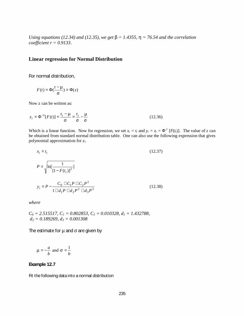
235
Using equations (12.34) and (12.35), we get β = 1.4355, η = 76.54 and the correlationcoefficient r = 0.9133.
Linear regression for Normal Distribution
For normal distribution,
)()()( zttF Φ=−
Φ=σ
µ
Now z can be written as:
σµ
σσµ
−=−
=Φ= − iii
tttFz )]([1 (12.36)
Which is a linear function. Now for regression, we set xi = ti and yi = zi = Φ-1 [F(ti)]. The value of z canbe obtained from standard normal distribution table. One can also use the following expression that givespolynomial approximation for zi.
ii tx = (12.37)
])](1[
1ln[2
itFP
−=
33
221
2210
1 PdPdPdPCPCC
Pyi+++
++−= (12.38)
where
C0 = 2.515517, C1 = 0.802853, C2 = 0.010328, d1 = 1.432788, d2 = 0.189269, d3 = 0.001308
The estimate for µ and σ are given by
ba
−=µ andb1
=σ
Example 12.7
Fit the following data into a normal distribution
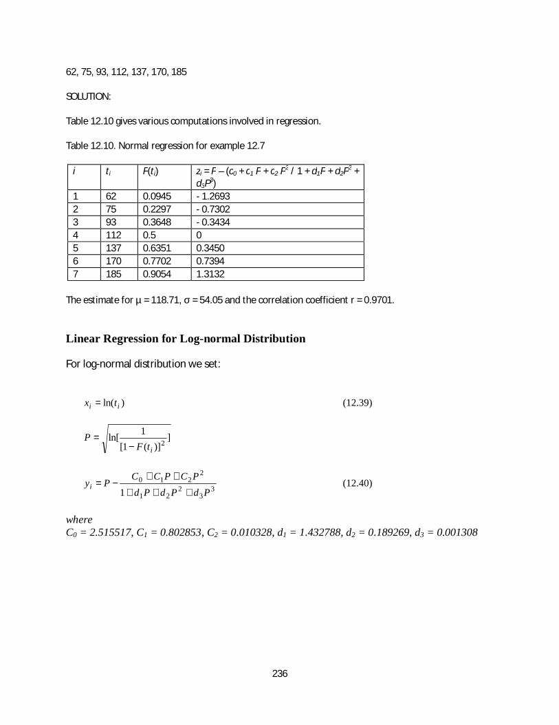
236
62, 75, 93, 112, 137, 170, 185
SOLUTION:
Table 12.10 gives various computations involved in regression.
Table 12.10. Normal regression for example 12.7
i ti F(ti) zi = P – (c0 + c1 P + c2 P2 / 1 + d1P + d2P2 +d3P3)
1 62 0.0945 - 1.26932 75 0.2297 - 0.73023 93 0.3648 - 0.34344 112 0.5 05 137 0.6351 0.34506 170 0.7702 0.73947 185 0.9054 1.3132
The estimate for µ = 118.71, σ = 54.05 and the correlation coefficient r = 0.9701.
Linear Regression for Log-normal Distribution
For log-normal distribution we set:
)ln( ii tx = (12.39)
])](1[
1ln[2
itFP
−=
33
221
2210
1 PdPdPdPCPCC
Pyi+++
++−= (12.40)
whereC0 = 2.515517, C1 = 0.802853, C2 = 0.010328, d1 = 1.432788, d2 = 0.189269, d3 = 0.001308
237
Total Cost of Ownership (TCO) and Life Cycle CostModels
Prof. U Dinesh KumarIndian Institute of Management Bangalore
238
CONTENTS
1. Life Cycle Cost and Total Cost of Ownership 31.1 Introduction. 31.2 Initial Capital Cost 51.3 Life of the Asset 51.4 The Discount Rate 61.5 Operation and Maintenance Cost 61.6 Disposal Cost 61.7 Uncertainties and Sensitivity Analysis 61.8 Summary 7
2. Survey of Existing Literature 092.1 Life Cycle Cost/Total Cost of Ownership Concept 092.2 Definitions of Life Cycle Cost/Cost of Ownership 122.3 Life Cycle Cost Technique 132.4 Review of Life Cycle Cost Models 162.5 Taylor s LCC Model 232.6 Raymer s LCC Model 252.7 Roskam s LCC Model 252.8 Fabrycky and Blanchard s LCC Model 262.9 Burn s Life Cycle Cost Model 282.10 PRICE Life Cycle Costing System 282.11 Equipment Designer s Cost Analysis System (EDCAS) 282.12 LCC Models Using Markov Chain 302.13 LCC Models for Labour Factor 312.14 LCC Models in Designing for Logistic Support 312.15 Applications of LCC/Cost of Ownership Models 34
References 35

239
240
1. Life Cycle Cost and Total Cost of Ownership___________________________________________
1.1 Introduction
“Value for Money” has become one of the important criteria in an increasingly competitive
business environment. Life Cycle Cost (LCC) and the Total Cost of Ownership (TCO) are two important
financial measures that are used for decision making in acquisitions. From its origins in defence
equipment procurement in the US in early 1960s, the use of life cycle cost and cost of ownership has
extended to other areas of the public and private sectors. LCC and TCO are being used to assist in
decision-making, budget planning, cost control, and range of other activities that occur over the life of
complex technological equipment.
It is important to consider the difference between LCC and TCO. LCC analysis is applied
routinely to military projects. In the military sector the consumer, by funding the project and operating
the related product, essentially bears the total life cycle cost covering the major cost elements in all
stages of a product’s life cycle. The term LCC analysis is rarely used in the commercial sector. Instead,
the main focus is on TCO where related costs, covering acquisition (purchase or lease), operation,
maintenance and support are borne by the customer. In addition, the customer can also incur costs
when the product is not available for use, that is, ‘down time costs’.
The objectives of LCC/TCO are (Flanagan and Norman, 1983):
Ø To enable investment options to be more effectively evaluated.
Ø To consider the impact of all costs rather than only the initial capital costs.
Ø To assist in the effective management of completed projects.

241
Ø To facilitate choice between competing alternatives.
In the Defence industry the system’s life cycle is divided into various phases, which allow proper
planning and control of a project. The number of phases depend on the nature of the project, purpose
and whether they are applied to commercial, military or space projects (Knotts, 1998). Commonly used
phases are:
1. Requirements (Functional Specification).
2. Concept/Feasibility Studies.
3. Design and Development.
4. Production.
5. Testing and Certification.
6. Operation, Maintenance and Support.
7. Disposal
It is reported by the US Department of Defence that 70% of weapon system life cycle cost is
committed by the end of concept studies, 85% by the end of system definition and 95% by the end of
full scale development. The US Department of Defence has formally used the concept of life cycle cost
in weapon system acquisition since the early 1960s through life cycle costing and life cycle cost analysis.
The cost of ownership approach identifies all future costs and reduces them to their present
value by use of the discounting techniques through which the economic worth of a product or product
options can be assessed. In order to achieve these objectives the following elements of cost of
ownership have been identified (Woorward, 1997):
Ø Initial capital costs
Ø Life of the asset
Ø The discount rate
242
Ø Operating and maintenance costs
Ø Disposal cost
Ø Uncertainty and sensitivity analysis
1.2 Initial capital costs
The initial capital costs can be divided into three sub-categories of cost namely: (1) purchase costs,
(2) acquisition/finance costs, and (3) installation/commissioning/training costs. Purchase costs will
include assessment of items such as land, buildings, fees, and equipment. Finance costs include
alternative sources of funds. Basically, the initial capital cost category includes all the costs of buying
the physical asset and bringing it into operation.
1.3 Life of the Asset
The estimated life of an asset has a major influence on life cycle cost analysis. Ferry et al (1991) has
defined the following five possible determinants of an asset’s life expectancy:
Functional life – the period over which the need for the asset is anticipated.
Physical life – the period over which the asset may be expected to last physically, to when
replacement or major rehabilitation is physically required.
Technological life – the period until technical obsolescence dictates replacement due to the
development of a technologically superior alternative.
Economic life – the period until economic obsolescence dictates replacement with a lower cost
alternative.
Social and legal life – the period until human desire or legal requirement dictates replacement.
1.4 The discount rate
243
As the cost of ownership is discounted to their present value, selection of a suitable discount rate is
crucial for TCO analysis. A high discount rate will tend to favour options with low capital cost, short life
and high recurring cost, whilst a low discount rate will have the opposite effect.
1.5 Operations and Maintenance Costs
Cost of ownership, in many cases, is about operation and maintenance cost. Estimation of
operation and maintenance costs is the essential to minimise the total cost of ownership of the asset. In
the whole of TCO analysis, estimation of operation and maintenance is the most challenging task.
1.6 Disposal cost
This is the cost incurred at the end of as asset’s working life in disposing of the asset. The
disposal cost would include the cost of demolition, scrapping or selling the asset.
1.7 Uncertainties and Sensitivity Analysis
LCC/TCO is highly dependent on the assumptions and estimates made whist collecting data.
Even though it is possible to improve the quality of these estimates, there is always an element of
uncertainty associated with these estimates and assumptions. Macedo et al (1978) identifies the
following five major sources of uncertainty:
1. Differences between the actual and expected performance of the system could affect future
operation and maintenance cost.
2. Changes in operational assumptions arising from modifications in user activity.
3. Future technological advances that could provide lower cost alternatives and hence shorten the
economic life of any system/subsystem.
4. Changes in the price levels of major resources such as energy or manpower, relative to other
resources can affect future alteration costs.
244
5. Error in estimating relationships, price rates for specific resources and the rate of inflation in
overall costs from the time of estimation to the availability of the asset.
While undertaking a LCC/TCO analysis, there may be some key parameters about which uncertainty
exists, usually because of the inadequacy of the input data. Blanchard (1972) suggested the following
should be the subject of sensitivity analysis:
Ø Frequency of the maintenance factor.
Ø Variation of the asset’s utilization or operating time.
Ø Extent of the system’s self-diagnostic capability.
Ø Variation of corrective maintenance hours per operating hour.
Ø Product demand rate.
Ø The discount rate
1.8 Summary
In this chapter, we looked at the concept of Life Cycle Cost and Cost of Ownership and the
factors that influence LCC and TCO as described in the literature. In the next chapter we survey the
existing LCC/TCO models, methodologies, practices and techniques available in the literature and its
applications and limitations. The models that have direct application for assessing the total cost of
ownership of airborne military equipment are highlighted.
245
53. 2. SURVEY OF EXISTING LITERATURE
Although a considerable body of literature relating to life cycle cost and cost of ownership has
been developed over the past four decades, much of the published material has emanated from
practitioners (Nicholas, 1999). Publications by practitioners have tended to consist of general guidelines
and a substantial amount of technical reports in the form of technical reports and conference papers,
detailing the development and application of specific models and modeling techniques. Most of these
papers lacked rigor that one can expect from academic publications. Much fewer in number, academic
publications have taken the form of text books which present tools and techniques of analysis (Dhillon
1989, Fabrycky and Blanchard 1991) and Journal publications, which tend to consider very specific
technical aspects of LCC and TCO. We have grouped the literature under different classification, namely,
(1) Publications on LCC/TCO concepts, (2) Publications on LCC models, (3) Publications on TCO models,
and (4) Publications on LCC/TCO applications.
2.1 Life Cycle Cost/Total Cost of Ownership Concept
Asiedu and Gu (1998) in their paper titled, ‘Product life cycle cost analysis – state of the art
review,’ provides an in-depth analysis of several issues of the life cycle cost. The paper discusses issues
such as (1) life cycle approach to design; (2) life cycle cost analysis, and (3) cost analysis models. They
point out that LCC analysis should not be seen as an approach for determining the cost of the system
but as an aid to design decision-making. The use of life cycle cost analysis and cost of ownership should
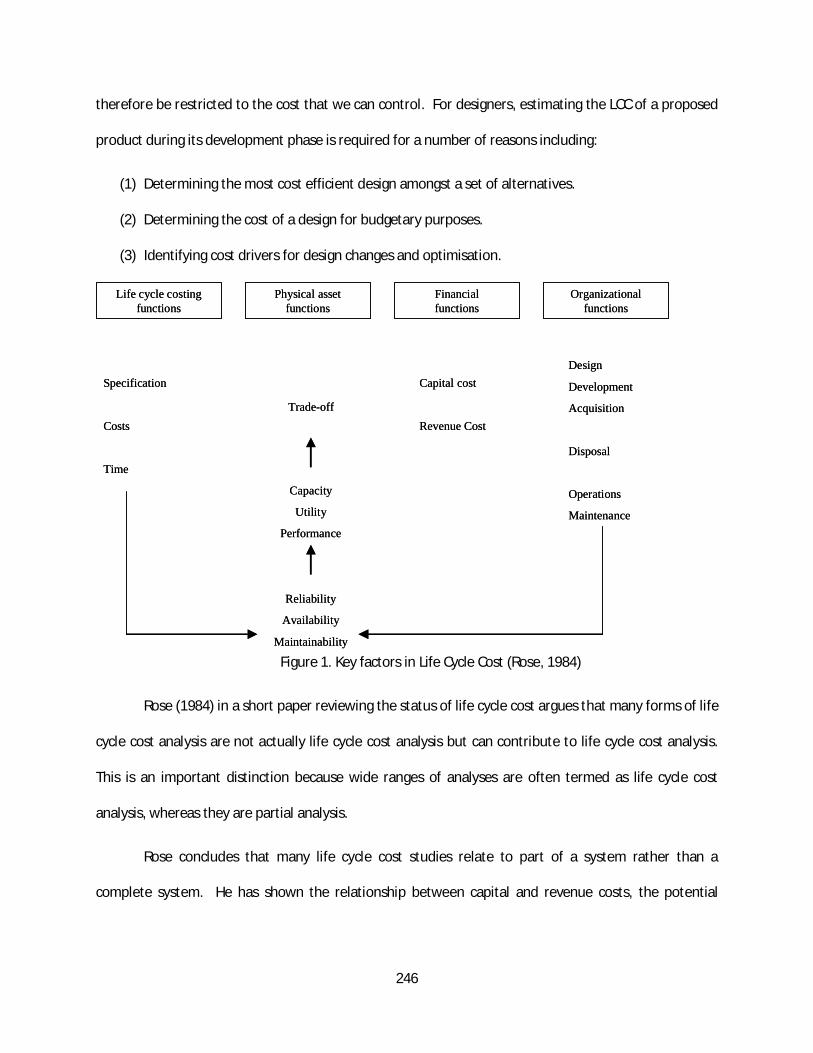
246
therefore be restricted to the cost that we can control. For designers, estimating the LCC of a proposed
product during its development phase is required for a number of reasons including:
(1) Determining the most cost efficient design amongst a set of alternatives.
(2) Determining the cost of a design for budgetary purposes.
(3) Identifying cost drivers for design changes and optimisation.
Figure 1. Key factors in Life Cycle Cost (Rose, 1984)
Rose (1984) in a short paper reviewing the status of life cycle cost argues that many forms of life
cycle cost analysis are not actually life cycle cost analysis but can contribute to life cycle cost analysis.
This is an important distinction because wide ranges of analyses are often termed as life cycle cost
analysis, whereas they are partial analysis.
Rose concludes that many life cycle cost studies relate to part of a system rather than a
complete system. He has shown the relationship between capital and revenue costs, the potential
Life cycle costingfunctions
Physical assetfunctions
Financialfunctions
Organizationalfunctions
Specification
Costs
Time
Trade-off
Capital cost
Revenue Cost
Design
Development
Acquisition
Disposal
Operations
Maintenance
Reliability
Availability
Maintainability
Capacity
Utility
Performance
Life cycle costingfunctions
Physical assetfunctions
Financialfunctions
Organizationalfunctions
Specification
Costs
Time
Trade-off
Capital cost
Revenue Cost
Design
Development
Acquisition
Disposal
Operations
Maintenance
Reliability
Availability
Maintainability
Capacity
Utility
Performance
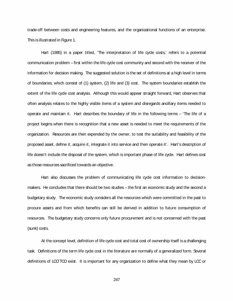
247
trade-off between costs and engineering features, and the organizational functions of an enterprise.
This is illustrated in Figure 1.
Hart (1985) in a paper titled, ‘The interpretation of life cycle costs,’ refers to a potential
communication problem – first within the life cycle cost community and second with the receiver of the
information for decision making. The suggested solution is the set of definitions at a high level in terms
of boundaries, which consist of (1) system, (2) life and (3) cost. The system boundaries establish the
extent of the life cycle cost analysis. Although this would appear straight forward, Hart observes that
often analysis relates to the highly visible items of a system and disregards ancillary items needed to
operate and maintain it. Hart describes the boundary of life in the following terms – ‘The life of a
project begins when there is recognition that a new asset is needed to meet the requirements of the
organization. Resources are then expended by the owner, to test the suitability and feasibility of the
proposed asset, define it, acquire it, integrate it into service and then operate it’. Hart’s description of
life doesn’t include the disposal of the system, which is important phase of life cycle. Hart defines cost
as those resources sacrificed towards an objective.
Hart also discusses the problem of communicating life cycle cost information to decision-
makers. He concludes that there should be two studies – the first an economic study and the second a
budgetary study. The economic study considers all the resources which were committed in the past to
procure assets and from which benefits can still be derived in addition to future consumption of
resources. The budgetary study concerns only future procurement and is not concerned with the past
(sunk) costs.
At the concept level, definition of life cycle cost and total cost of ownership itself is a challenging
task. Definitions of the term life cycle cost in the literature are normally of a generalized form. Several
definitions of LCC/TCO exist. It is important for any organization to define what they mean by LCC or
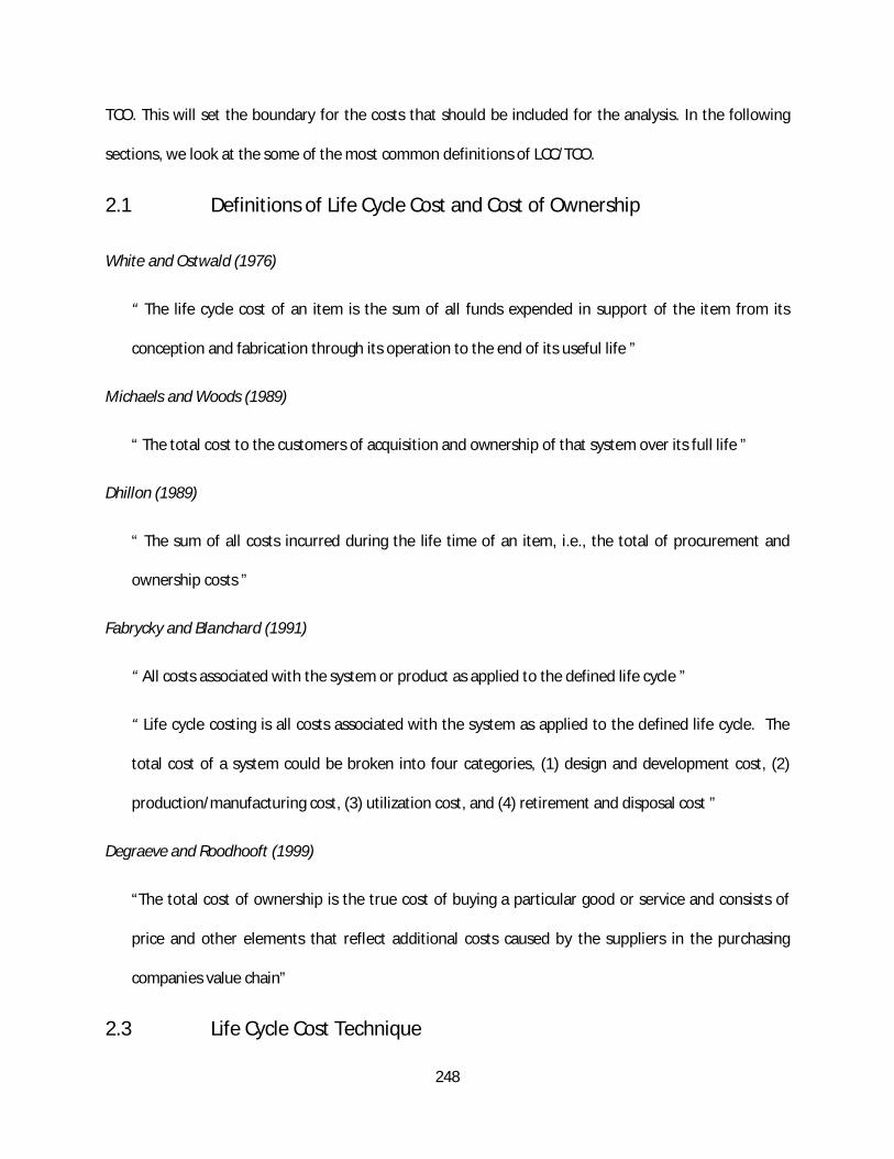
248
TCO. This will set the boundary for the costs that should be included for the analysis. In the following
sections, we look at the some of the most common definitions of LCC/TCO.
2.1 Definitions of Life Cycle Cost and Cost of Ownership
White and Ostwald (1976)
“ The life cycle cost of an item is the sum of all funds expended in support of the item from its
conception and fabrication through its operation to the end of its useful life ”
Michaels and Woods (1989)
“ The total cost to the customers of acquisition and ownership of that system over its full life ”
Dhillon (1989)
“ The sum of all costs incurred during the life time of an item, i.e., the total of procurement and
ownership costs ”
Fabrycky and Blanchard (1991)
“ All costs associated with the system or product as applied to the defined life cycle ”
“ Life cycle costing is all costs associated with the system as applied to the defined life cycle. The
total cost of a system could be broken into four categories, (1) design and development cost, (2)
production/manufacturing cost, (3) utilization cost, and (4) retirement and disposal cost ”
Degraeve and Roodhooft (1999)
“The total cost of ownership is the true cost of buying a particular good or service and consists of
price and other elements that reflect additional costs caused by the suppliers in the purchasing
companies value chain”
2.3 Life Cycle Cost Technique
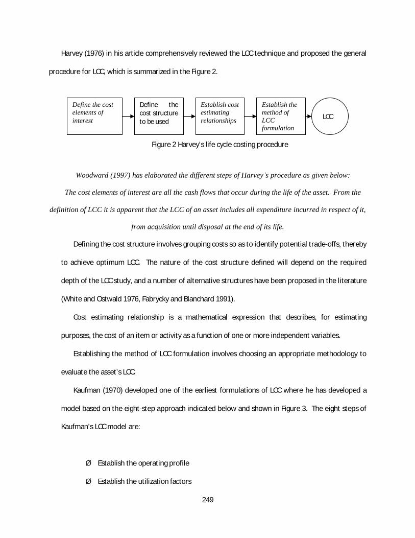
249
Harvey (1976) in his article comprehensively reviewed the LCC technique and proposed the general
procedure for LCC, which is summarized in the Figure 2.
Figure 2 Harvey’s life cycle costing procedure
Woodward (1997) has elaborated the different steps of Harvey s procedure as given below:
The cost elements of interest are all the cash flows that occur during the life of the asset. From the
definition of LCC it is apparent that the LCC of an asset includes all expenditure incurred in respect of it,
from acquisition until disposal at the end of its life.
Defining the cost structure involves grouping costs so as to identify potential trade-offs, thereby
to achieve optimum LCC. The nature of the cost structure defined will depend on the required
depth of the LCC study, and a number of alternative structures have been proposed in the literature
(White and Ostwald 1976, Fabrycky and Blanchard 1991).
Cost estimating relationship is a mathematical expression that describes, for estimating
purposes, the cost of an item or activity as a function of one or more independent variables.
Establishing the method of LCC formulation involves choosing an appropriate methodology to
evaluate the asset’s LCC.
Kaufman (1970) developed one of the earliest formulations of LCC where he has developed a
model based on the eight-step approach indicated below and shown in Figure 3. The eight steps of
Kaufman’s LCC model are:
Ø Establish the operating profile
Ø Establish the utilization factors
Define the costelements ofinterest
Define thecost structureto be used
Establish costestimatingrelationships
Establish themethod ofLCCformulation
LCC
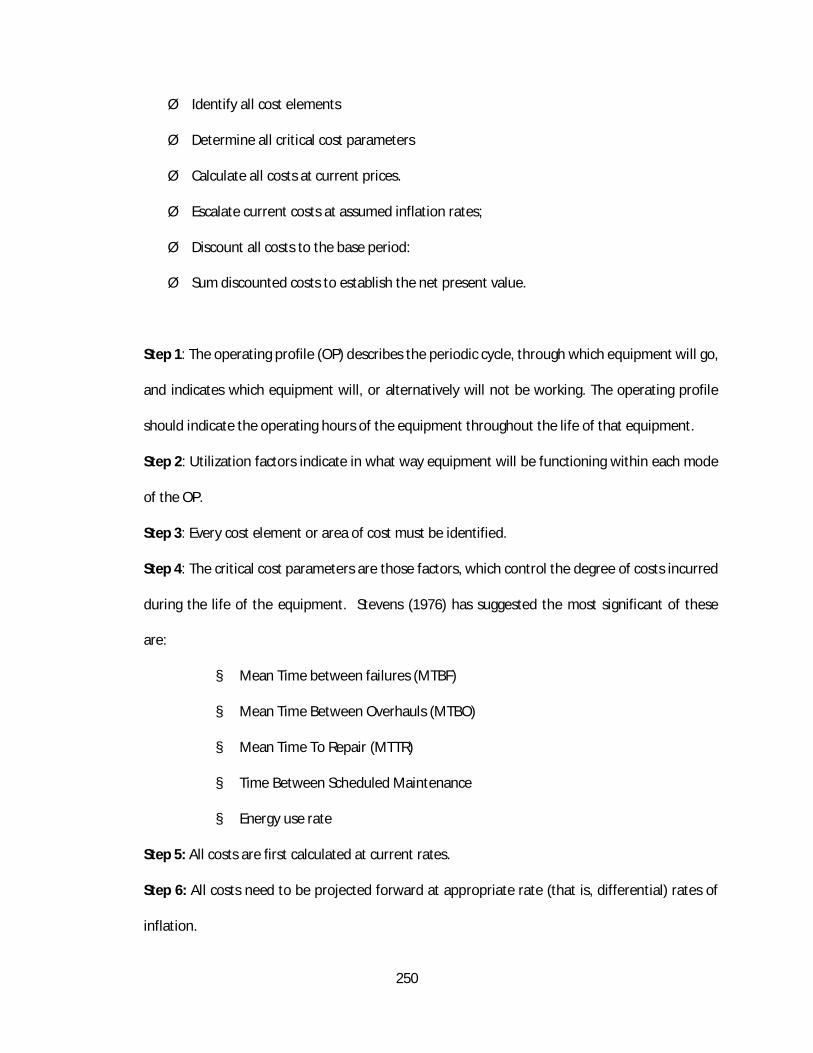
250
Ø Identify all cost elements
Ø Determine all critical cost parameters
Ø Calculate all costs at current prices.
Ø Escalate current costs at assumed inflation rates;
Ø Discount all costs to the base period:
Ø Sum discounted costs to establish the net present value.
Step 1: The operating profile (OP) describes the periodic cycle, through which equipment will go,
and indicates which equipment will, or alternatively will not be working. The operating profile
should indicate the operating hours of the equipment throughout the life of that equipment.
Step 2: Utilization factors indicate in what way equipment will be functioning within each mode
of the OP.
Step 3: Every cost element or area of cost must be identified.
Step 4: The critical cost parameters are those factors, which control the degree of costs incurred
during the life of the equipment. Stevens (1976) has suggested the most significant of these
are:
§ Mean Time between failures (MTBF)
§ Mean Time Between Overhauls (MTBO)
§ Mean Time To Repair (MTTR)
§ Time Between Scheduled Maintenance
§ Energy use rate
Step 5: All costs are first calculated at current rates.
Step 6: All costs need to be projected forward at appropriate rate (that is, differential) rates of
inflation.
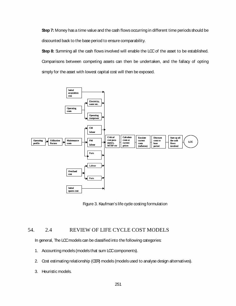
251
Step 7: Money has a time value and the cash flows occurring in different time periods should be
discounted back to the base period to ensure comparability.
Step 8: Summing all the cash flows involved will enable the LCC of the asset to be established.
Comparisons between competing assets can then be undertaken, and the fallacy of opting
simply for the asset with lowest capital cost will then be exposed.
Figure 3. Kaufman’s life cycle costing formulation
54. 2.4 REVIEW OF LIFE CYCLE COST MODELS
In general, The LCC models can be classified into the following categories:
1. Accounting models (models that sum LCC components).
2. Cost estimating relationship (CER) models (models used to analyse design alternatives).
3. Heuristic models.
Parts
Labour
Parts
Operatingprofile
UtilizationFactors
Maintenancecosts
PM
labour
Criticalcost para-meters,MTBF ete
Calculatecosts atcurrentprices
Escalatecurrentcosts(inflation)
Discountcosts tobaseperiod
Sum up allthe cashflowsinvolved
LCC
CM
labour
Operatingmanpower
Electricity,water etc.
Operatingcosts
Initialspares cost
Initialacquisitioncost
Overhaulcost
Parts
Labour
Parts
Operatingprofile
UtilizationFactors
Maintenancecosts
PM
labour
Criticalcost para-meters,MTBF ete
Calculatecosts atcurrentprices
Escalatecurrentcosts(inflation)
Discountcosts tobaseperiod
Sum up allthe cashflowsinvolved
LCC
CM
labour
Operatingmanpower
Electricity,water etc.
Operatingcosts
Initialspares cost
Initialacquisitioncost
Overhaulcost
Operatingprofile
UtilizationFactors
Maintenancecosts
PM
labour
Criticalcost para-meters,MTBF ete
Calculatecosts atcurrentprices
Escalatecurrentcosts(inflation)
Discountcosts tobaseperiod
Sum up allthe cashflowsinvolved
LCCLCC
CM
labour
Operatingmanpower
Electricity,water etc.
Operatingcosts
Initialspares cost
Initialacquisitioncost
Overhaulcost
252
4. Failure free warranty models (models used to analyse warranty periods)
5. Reliability models (used to apportion reliability and maintainability), and
6. Economic analysis models (models dealing with general cost effectiveness).
However, Sherif and Kolarik (1981) classify LCC models into three general forms: (1) conceptual, (2)
analytical models, and (3) heuristic models. Conceptual models consist of a set of hypothetical
relationships expressed in a qualitative framework. Conceptual models are generally constructed at
macro level. Analytic models consist of a set of mathematical relationships, which are used to describe a
certain aspect of the system. Such models range from models covering very specific aspects of a system
to models, which address total system life cycle cost.
Gupta (1983) identifies three types of analytic models: (1) design trade-off models, (2) total cost
models, and (3) logistic support models. Design trade-off models relate to the design phase of the life
cycle cost and attempt to minimise cost to meet a given value of design parameters such as reliability
and availability to maximize the value of design parameters for given cost constraints. Total cost models
are termed true life cycle cost models and usually encompass the total life of the system. They attempt
to minimize the total life cycle cost of the system while maximizing its performance and effectiveness by
evaluating various parameters such as reliability, maintainability, availability etc, which affect life cycle
cost. Logistic support models are concerned with the operations phase of the life cycle. Usually the
objective of such models is to determine costs for alternative support plans and effect on the system’s
effectiveness. They reflect operations cost parameters as variable costs and research, development,
test and evaluation and acquisitions costs as fixed costs. These models are inconsistent in that design
parameters such as reliability and maintainability heavily influence operations costs and therefore fall
short of determining optimal life cycle cost.
Dhillon (1989) simply divides life cycle cost models into two forms: (1) general life cycle cost models,
and (2) specific life cycle cost models. General life cycle cost models are not related to any specific
253
equipment or system whereas specific life cycle cost models have been developed for particular types of
equipment or system. Given the specific interrelationships and interactions of a particular system, the
application of general models is clearly limited. Recently, Daniel (1991) has classified life cycle cost
models into two broad categories: (1) accounting models which attempt to assemble and distribute
costs, determined elsewhere so as to describe the total cost of a system, and (2) predictive models
which are used to forecast the values of the various cost elements required as input to the accounting
models.
Noble and Tanchoco (1990) developed a conceptual framework for concurrent design and economic
justification of the system. A prototype implementation was developed to explore the usefulness of
the design justification concept. Actual data from the design of an electromagnetic/radio frequency
shield, a component in electrical metering equipment, was used to demonstrate the model.
Woodward (1997) in his paper titled, ‘Life Cycle Costing – Theory, Information Acquisition and
Application,’ presented a case on total cost of ownership on South Yorkshire Passenger Transport
(SYPT). SYPT’s main activity is the provision of passenger transport services by road. It’s fixed assets
were worth $ 43,327,500 out of which the passenger vehicles accounted for about 17,662,500. The
company purchases vehicles that form a major part of the capital expenditure, on a regular basis
and the decision to purchase them is based on the LCC technique. The estimated life cycle costs are
discounted at an assumed monetary cost of capital of 15%, after including a standard inflation rate
assumed over the life of the asset. If the two alternatives have similar discounted costs, then a
choice will be made by the financial director taking into account non-financial factors such as the
credibility, reliability etc. of the suppliers. Although, the case was on passenger transport by road,
the concept is valid for any system, including airborne defence equipment.
Degraeve and Roodhooft (1999) developed a mathematical programming model that uses total cost
of ownership information to select suppliers and determine order quantities over a multi-period time
254
horizon. The total cost of ownership quantifies all costs associated with purchasing process and is based
on the activities and cost drivers determined by an Activity Based Costing (ABC) system. They have also
discussed a case on the purchasing problem of heating electrodes at Cockerill Sambre, a Belgian
multinational steel producer. In this case, quality issues accounted for more than 70% of the total cost
of ownership making the quality of the supplier a critical success factor in the supplier selection process.
LCC model can be a simple series of cost estimation relationships (CERs). LCC analysis during the
conceptual or preliminary design phases may require the use of basic accounting techniques (Fabrycky
and Blanchard, 1991). The most important task in LCC modeling is the construction of Cost Breakdown
Structure (CBS), which shows various cost categories that combine to provide the total cost. Cost
breakdown structure should exhibit the following basic characteristics (Blanchard et al 1995):
1. All system cost elements must be considered.
2. Cost categories are generally identified with a significant level of activity or some major item of
hardware.
3. The cost structure and categories should be coded in such a manner as to allow for the analysis
of certain specific areas of interest (e.g., system operation, energy consumption, equipment
design, spares, maintenance personnel and support, maintenance equipment and facilities). In
some instances, the analyst may wish to pursue a designated area in depth while covering other
areas with gross top-level estimates. This will certainly occur from time to time as a system
evolves through the different phases of its life cycle.
4. When related to a specific program, the cost structure should be compatible (through cross-
indexing, coding etc.) with the contract work breakdown structure (WBS) and with management
accounting procedures used in collecting costs.
5. For program, where subcontracting is prevalent, it is often desirable and necessary to separate
supplier costs (i.e., initial bid price and follow-on program costs) from other costs. The cost
255
structure should allow for the identification of specific work packages that require close
monitoring and control.
An example of a cost breakdown structure adopted from Blanchard (1991) is shown in Figure 4.
Referring to Figure 4, costs may be accumulated at different levels depending on the areas of interest
and the depth of detail required. Most of the LCC models can be a simple series of cost estimation
relationships. Estimating models used in industry can be broadly classified as parametric models,
analogous models and detailed models (Asiedu and Gu, 1998).
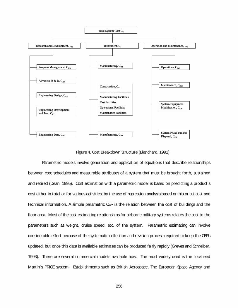
256
Figure 4. Cost Breakdown Structure (Blanchard, 1991)
Parametric models involve generation and application of equations that describe relationships
between cost schedules and measurable attributes of a system that must be brought forth, sustained
and retired (Dean, 1995). Cost estimation with a parametric model is based on predicting a product’s
cost either in total or for various activities, by the use of regression analysis based on historical cost and
technical information. A simple parametric CER is the relation between the cost of buildings and the
floor area. Most of the cost estimating relationships for airborne military systems relates the cost to the
parameters such as weight, cruise speed, etc. of the system. Parametric estimating can involve
considerable effort because of the systematic collection and revision process required to keep the CERs
updated, but once this data is available estimates can be produced fairly rapidly (Greves and Schreiber,
1993). There are several commercial models available now. The most widely used is the Lockheed
Martin’s PRICE system. Establishments such as British Aerospace, The European Space Agency and
Total System Cost CT
Research and Development, CR Investment, CI Operation and Maintenance, CO
Program Management, CRM
Advanced R & D, CRR
Engineering Design, CRE
Engineering Developmentand Test, CRT
Engineering Data, CRD
Manufacturing, CIM
Construction, CIC
--------------------------------
Manufacturing Facilities
Test Facilities
Operational Facilities
Maintenance Facilities
Manufacturing, CIM
Operations, COO
Maintenance, COM
System/EquipmentModification, CON
System Phase-out andDisposal, COP
257
NASA use PRICE system. However, it is not recommended for estimating the cost of products that utilize
new technologies.
55. ANALOGOUS MODELS
Cost estimating made by analogy identifies a similar product or component and adjusts for
differences between it and the target product (Shields and Young 1991). The effectiveness of this
method depends heavily on an ability to identify correctly the differences between the case in hand and
those deemed to be comparable. The main disadvantage of estimating by analogy is the high degree of
judgment required.
56. DETAILED MODELS
Detailed models use estimates of labour times and rates and also material quantities and prices
to estimate the direct costs of a product or activity (Shields and Young, 1991). An allocation rate is then
used to allow for indirect/overhead costs. This is known as bottom-up estimating and is widely used to
allow indirect/overhead costs. It is the most time consuming and costly approach and requires a very
detailed knowledge of the product and processes. However, the most accurate cost estimates can be
made using this approach. The method involves (Asiedu and Gu, 1998) estimation the time needed
to perform an activity and the hourly rates for the man and machine, and then multiply times and rates
to get costs. Time standards can be industry standards, in-house standards or based on expert guesses.
In-house standards are the best but most difficult to develop. Industrial time standards for production
operations exist for many common tasks.
258
57. IN THE NEXT FEW SECTIONS WE DESCRIBE FEW LCC
MODELS THAT ARE POPULAR AMONG PRACTITIONERS THAT CAN
BE USED FOR ESTIMATION OF LIFE CYCLE COST/COST OF
OWNERSHIP OF AIRBORNE MILITARY EQUIPMENT.
58. 2.5 TAYLOR S LCC MODEL
Taylor’s model focuses on the capital and revenue costs. Taylor claims that in any discussion of
trade-offs between initial and subsequent costs, a point that is frequently made is that there is a major
distinction between initial capital costs and revenue costs. It is claimed that companies and public
bodies faced with limited capital budget or cost limits do not have the facility to increase initial capital
costs on the chance that there will be future revenue gains. However, Taylor claims that the distinction
between revenue expenditure and capital is an accounting one which doesn’t affect the life cycle cost
concept based on the cash flows throughout the life of the asset.
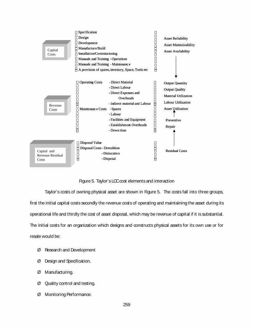
259
Figure 5. Taylor’s LCC cost elements and interaction
Taylor’s costs of owning physical asset are shown in Figure 5. The costs fall into three groups,
first the initial capital costs secondly the revenue costs of operating and maintaining the asset during its
operational life and thirdly the cost of asset disposal, which may be revenue of capital if it is substantial.
The initial costs for an organization which designs and constructs physical assets for its own use or for
resale would be:
Ø Research and Development
Ø Design and Specification.
Ø Manufacturing.
Ø Quality control and testing.
Ø Monitoring Performance.
CapitalCosts
etcToolsSpace,inventory,spares,ofprovisionAeMaintenanc-TrainingandManuals
Operations-TrainingandManualsioningon/CommissInstallati
e/BuildManufacturtDevelopmen
DesignionSpecificat
Down time-OverheadsentEstablishm-
EquipmentandFacilities-Labour-Spares-CostseMaintenanc
LabourandmaterialIndirect-Overheads
andExpensesDirect-LabourDirect-MaterialDirect-CostsOperating
RevenueCosts
Capital andRevenue ResidualCosts
Disposal-nDislocatio-
Demolition-CostsDisposalValueDisposal
Residual Costs
Preventive
Repair
Output Quantity
Output Quality
Material Utilization
Labour Utilization
Asset Utilization
Asset Reliability
Asset Maintainability
Asset AvailabilityCapitalCostsCapitalCosts
etcToolsSpace,inventory,spares,ofprovisionAeMaintenanc-TrainingandManuals
Operations-TrainingandManualsioningon/CommissInstallati
e/BuildManufacturtDevelopmen
DesignionSpecificat
Down time-OverheadsentEstablishm-
EquipmentandFacilities-Labour-Spares-CostseMaintenanc
LabourandmaterialIndirect-Overheads
andExpensesDirect-LabourDirect-MaterialDirect-CostsOperating
RevenueCostsRevenueCosts
Capital andRevenue ResidualCosts
Capital andRevenue ResidualCosts
Disposal-nDislocatio-
Demolition-CostsDisposalValueDisposal
Residual Costs
Preventive
Repair
Output Quantity
Output Quality
Material Utilization
Labour Utilization
Asset Utilization
Asset Reliability
Asset Maintainability
Asset Availability
260
The second group of costs are incurred during the operational life of the asset and this would
include the costs of: operating the assets including the labour, materials, tools, fixtures and overheads,
maintenance including spares and labour. Finally there are disposal costs which include costs of
demolition and removal, dislocation of existing production capacity. Against this may be any disposal
value of the physical asset.
2.6 Raymer’s LCC Model
Raymer’s life cycle costing model is based on the Development and Procurement Costs of
Aircraft (DAPCA IV) model developed by the Rand Corporation. The Rand corporation developed several
cost estimation relationships for estimating various costs for all departments including engineering,
tooling, manufacturing and quality control groups. DAPCA assumes a ten-year product life, which also is
an industry standard. Rand Corporation claims that DAPCA, coupled with appropriate factors is accurate
to within +/- 5% of actual costs.
2.7 Roskam LCC Model
Roskam model divides the LCC into four major categories: (1) Research and Development, test and
evaluation, (2) Program acquisition cost that includes manufacturing cost and manufacturer’s profit, (3)
Operating cost, and (4) Disposal cost. The expression for LCC is given by the equation:
DOMACRDTE CCCCLCC +++=
(1)
Where, CRDTC is the R&D, test and evaluation cost, CAC is the acquisition cost, COM is the operation
and maintenance cost and CD is the disposal cost.
261
R&D cost is further broken into cost elements such as: (1) airframe engineering and design, (2) test
flight aircraft and flight test operations, (3) test & simulation facilities, (4) cost to finance. Each of these
cost elements is estimated using parametric methods using aircraft weight, maximum design speed, and
number of aircraft built. Similarly acquisition cost is calculated using parameters such as the number of
aircrafts manufactured, manufacturing cost, take-off weight, design cruise speed etc.
Operation costs are broken into the material costs, direct and in-direct personnel cost and logistic
support costs. The disposal cost is taken as 1% of the LCC cost. Roskam developed several cost
estimation relationships for estimation of the various costs given in above equation. Most of these
models were developed using weight of the aircraft as a dependent variable.
2.8 Fabrycky and Blanchard’s LCC Model
Fabrycky and Blanchard (1991) developed the detailed LCC model. The most important task in
their model is to develop the cost breakdown structure (CBS, shown in Figure 4). There is no method set
for breaking down the costs as long as the method used can be tailored to the specific application.
Primarily the cost is divided into the following four categories:
Ø Research and development
Ø Production and construction costs
Ø Operation and maintenance costs
Ø Retirement and disposal costs
Thus the total cost is (C) is calculated using the expression:
DOPR CCCCC +++=
(2)
Where,
262
CostDisposalandRetirementCCost,eMaintenancandOperationCCost,onConstructiandProductionCcost,D&RC
RO
PR
====
The total cost, C, includes all future costs associated with the acquisition, utilization, and
subsequent disposal of system equipment.
Research and development cost includes all costs associated with conceptual feasibility studies,
basic and advanced research and development, engineering design, fabrication and test of engineering
prototype models (hardware), and associated documentation. Also covers all related program
management functions. The R&D cost is given by:
RDRTRERRRM CCCCC ++++=RC
(3)
Where,
costdatagEngineerinCcostt/testdevelopmengEngineerinCcost,designgEngineerinC
Cost,D&RAdvancedCcost,managementProgramC
RD
RTRE
RRRM
===
==
Operations and maintenance cost includes all costs associated with the operation and
maintenance support of the system throughout the life cycle subsequent to the equipment delivery in
the field. Specific categories cover the cost of system operation, maintenance, sustaining logistic
support, equipment modifications. Thus, the operation and maintenance cost is given by:
OPONOMOOO CCCCC +++=
(4)
Where,
disposalsystemofCostCons,modificaticyclelifesystemofCostCe,maintenanccyclelifesystemofCostC,operationscyclelifesystemofCostC
OPON
OMOO
====
263
The costs in equations (2) – (4) can be further divided into various cost elements.
2.9 Burns Life Cycle Cost Model
Burns developed a cost estimation relationship for predicting life cycle cost of aircraft based on its
weight. Burns model is a simple extension of Roskam’s life cycle cost model. The model also includes
judgement factor for computing airframe-engineering hours for development and production. A
complete analysis of Burns model is presented in Jayakrishnan (2002).
2.10 PRICE Life Cycle Costing System
The PRICE system consists of parametric cost estimation models for predicting the life cycle cost of
weapon systems developed by the Lockheed Martin. The PRICE system’s tool includes a set of four
parametric cost estimation models, each with a different specialty area. The models consists of:
PRICE M: This model specifically addresses electronic module level hardware development and
production costs.
PRICE H: This model specifically addresses the costs associated with development and production of
hardware. This tool can use outputs of the PRICE M tool.
PRICE HL: This model uses data generated by PRICE H and calculates the hardware life-cycle costs,
including sparing for a deployment environment.
PRICE Software: This model estimates both development costs and life cycle support costs for
software.
2.11 Equipment Designer’s Cost Analysis System (EDCAS) Model
EDCAS is one of the popular commercial systems available for life cycle cost prediction. EDCAS is a
sequential model and is applicable for design to LCC in front-end design analysis. Over 500 government
264
and industry use the system worldwide. For example, U.S. Air Force uses EDCAS for aircraft and
airborne weapons and electronic systems.
2.12 LCC Models Using Markov Chain
Stump (1988) developed a LCC model based on Markov chains and illustrated the model for a
hypothetical remotely piloted vehicle (RPV). The Markov chain is used to estimate the operation,
maintenance and support costs. The model assumes that the system goes through a number of states.
For any state, the number of visits per cycle multiplied by the cost per visit and the expected life of the
RPV in cycles will yield a life cost for that state. Summing over all states will yield a total life cost. To
fully implement this life cycle cost methodology, the following information is needed:
1. A list of system states.
2. A list of transition probabilities from any state to any other state (zero if the states do not
communicate).
3. A list of the costs of entering the states.
4. The average number of visits per cycle for each state.
5. The expected life of the system.
6. Cost estimating relationships for computing costs.
The life cycle cost for state i is:
iii CaLLC ××=
(5)
Where, ai , is the state probability for state i and Ci is the average cost of entry into state i and L is
the expected life of the system. The total life cost of the RPV is simply the sum of the LCi for all states.
One of the major problems with Markov chain model is that the system is likely to have large number of
states.

265
2.13 LCC model for labour factor
Dahlen and Bolmsjo (1996) developed a life cycle cost model for the labour factor that covers
the costs for an employee over the whole employment cycle – from the requirement until retirement.
The costs are divided into three basic categories:
1. Employment costs: consisting of costs for recruiting, introduction and training of new employees
– to compare with acquisition costs such as projecting, installation and start-up of the new
equipment.
2. Operations costs: consisting of wages, and labour related overhead – to compare with
depreciation, maintenance and repairs.
3. Work environmental costs: consisting of a additional costs for absenteeism, rehabilitation and
pensions – to compare with costs for increased maintenance and repairs and finally to scrap the
equipment.
The basic categories of labour life cycle cost can be divided into: employment costs, operation costs
and work environmental costs. The employment costs can be divided into three major sub categories:
(1) recruitment costs, (2) additional productions costs and (3) education costs.
Operation costs are incurred when the employee is introduced and masters the work tasks, the
costs consists of wages and overheads. The third category, work environmental costs, includes costs for
absence, sickness benefits, rehabilitation costs and disability pension costs.
2.14 LCC Models in Designing for Logistic Support
Hatch and Bedinelli (1999) developed a model that carries out a concurrent optimization of a
product design and its associated manufacturing and logistic support system. The model is constructed
266
which links together the decisions associated with three major phases of the life cycle: product design,
manufacturing and logistic system design, production and field operation control. The model included
an optimization scheme that concurrently optimizes the decision variable of the linked model. The final
solution prescribed by the model is based on a multi-criteria value function formed from the individual
objectives of minimizing life cycle cost and maximizing availability. The model evaluates alternative
design solutions by calculating the associated operational availability as well as manufacturing and
logistic support costs. The two main performance measures can be combined into the following bi-
criteria model formulation:
Min Life Cycle Cost
Max System Availability
Subject to Product Design Requirements
2.15 Applications of LCC/Cost of Ownership Models
The literature survey carried out by Nicholas (1999) indicates that the term life-cycle cost/cost of
ownership is applied to varying forms of analysis, which are undertaken for a range of different
purposes. These applications can be broadly described as evaluation and decision-making, planning and
budgeting, cost management and control, project/program management and control, life-cycle
management, contracting, and marketing. These applications are shown in Table 1 in relation to recently
published papers.
Although life-cycle cost/cost of ownership is applied to analysis, which is used for a wide range of
purposes, it can be argued that in essence the analysis is being used to provide information for two
fundamental purposes - planning and control. Planning includes i) decision-making - the allocation of
267
resources for future periods through the identification, evaluation and selection of alternative courses
of action and ii) budgeting - the identification of means required to implement the selected courses of
action. Principal areas of control include cost control and contractual arrangements. Cost control
includes procedures to influence cost through design (Michaels and Wood, 1989) and throughout the
process of acquisition (US Department of Defense, 1996). Contractual arrangements are designed to
control cost through legal agreements. Contractual arrangements include guarantees for part of life-
cycle cost such as support cost (Baathe, 1995) and guarantees for total life cycle cost (Akselsson and
Burstrom, 1994). Planning and control are integrated through management which includes project and
program management during acquisition and much wider life-cycle management which extends to the
complete life-cycle of the system.
There is an important distinction to be made between the nature of the use of analysis to provide
information for planning and control. In planning, in both decision-making and budgeting, life-cycle cost
is used as an ex ante concept to predict future cost. In control, it is used as both an ex ante and an ex
post concept. It is used as an ex ante concept to establish targets or performance criteria but as an ex
post concept when monitoring and comparing cost performance in terms of planned cost against actual
cost. As indicated in the discussion of concepts of cost below, this will involve the application of
different concepts of cost.
Analysis using the concept of life-cycle cost is not only used for different purposes but also involves
different functional users. Examples of different users include policy-makers (Kirkpatrick, 1996),
managers (Riggs and Jones, 1990, Greene, 1991) and engineers (Various - see references and
bibliography). Policy-makers are involved in strategic decisions that involve the long-term
commitment of funds. Managers may be project managers or budget managers whose interest is
principally in control. Engineers may include design engineers, production engineers, systems
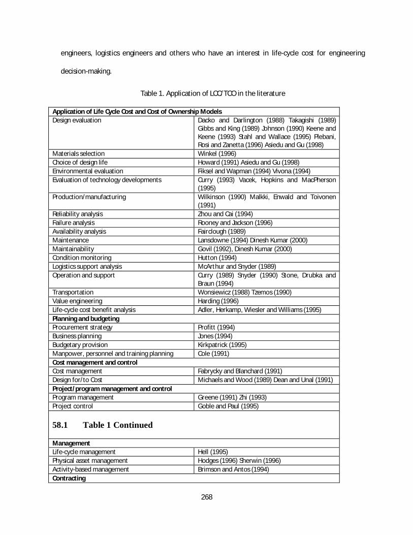
268
engineers, logistics engineers and others who have an interest in life-cycle cost for engineering
decision-making.
Table 1. Application of LCC/TCO in the literature
Application of Life Cycle Cost and Cost of Ownership ModelsDesign evaluation Dacko and Darlington (1988) Takagishi (1989)
Gibbs and King (1989) Johnson (1990) Keene andKeene (1993) Stahl and Wallace (1995) Plebani,Rosi and Zanetta (1996) Asiedu and Gu (1998)
Materials selection Winkel (1996)Choice of design life Howard (1991) Asiedu and Gu (1998)Environmental evaluation Fiksel and Wapman (1994) Vivona (1994)Evaluation of technology developments Curry (1993) Vacek, Hopkins and MacPherson
(1995)Production/manufacturing Wilkinson (1990) Malkki, Enwald and Toivonen
(1991)Reliability analysis Zhou and Cai (1994)Failure analysis Rooney and Jackson (1996)Availability analysis Fairclough (1989)Maintenance Lansdowne (1994) Dinesh Kumar (2000)Maintainability Govil (1992), Dinesh Kumar (2000)Condition monitoring Hutton (1994)Logistics support analysis McArthur and Snyder (1989)Operation and support Curry (1989) Snyder (1990) Stone, Drubka and
Braun (1994)Transportation Wonsiewicz (1988) Tzemos (1990)Value engineering Harding (1996)Life-cycle cost benefit analysis Adler, Herkamp, Wiesler and Williams (1995)Planning and budgetingProcurement strategy Profitt (1994)Business planning Jones (1994)Budgetary provision Kirkpatrick (1995)Manpower, personnel and training planning Cole (1991)Cost management and controlCost management Fabrycky and Blanchard (1991)Design for/to Cost Michaels and Wood (1989) Dean and Unal (1991)Project/program management and controlProgram management Greene (1991) Zhi (1993)Project control Goble and Paul (1995)
58.1 Table 1 Continued
ManagementLife-cycle management Hell (1995)Physical asset management Hodges (1996) Sherwin (1996)Activity-based management Brimson and Antos (1994)Contracting
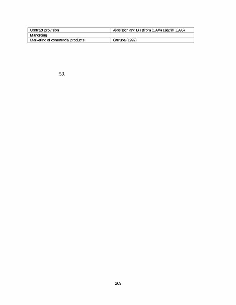
269
Contract provision Akselsson and Burstrom (1994) Baathe (1995)MarketingMarketing of commercial products Carruba (1992)
59.
270
List of References
Adler, D.J., Herkamp, J.A., Wiesler, J.R. and Williams, S.B. (1995) 'Life-Cycle Cost and Benefits of ProcessAutomation in Bulk Pharmaceuticals', ISA Transactions, Vol. 34, No. 2, pp. 133-139.
Ahmed, N. U. (1995) ‘A design and Implementation Model for Life Cycle Cost Management System’,Information and Management, Vol. 28, pp. 261-269.
Akselsson, H. and Burstrom, B. (1994) 'Life-Cycle Cost Procurement of Swedish State Railways High-Speed Train X2000', Proceedings of the Institution of Mechanical Engineers, Part F, Journal of Rail andRapid Transit, Vol. 208, No. 1, pp.51-59.
Asiedu, Y. and Gu, P. (1998) ‘Product Life Cycle Cost Analysis: State of the Art Review’, InternationalJournal of Production Economics, Vol. 36, No. 4, 883-908.
Baathe, O. (1995) ‘Life Cycle Management for the A/C JAS 39 Grippen’, Proceedings of 11th InternationalCongress, Society of Logistics Engineers, Stockholm, pp. 159-167.
Blanchard, B.S. (1972) ‘Design and Manage to Life Cycle Cost’, M/A Press, Oregon, USA.
Blanchard, B.S. (1986) Logistics Engineering and Management, 3rd Edition, Prentice-Hall, EnglewoodCliffs, New Jersey.
Blanchard, B.S. (1998) System Engineering Management, 2nd Edition, John Wiley, New York.
Blanchard, B.S. and Fabrycky, W.J. (1990) Systems Engineering and Analysis, 2nd Edition, Prentice-Hall,Englewood Cliffs, New Jersey.
Brimson, J.A. and Antos, J. (1994) Activity-Based Management, John Wiley, New York.
Burns, J. W. (1994) ‘Aircraft Cost Estimation Methodology and Value of a Pound Derivation forPreliminary Design Development Applications, SAWE Paper No. 2228, Long Beach, USA.
Carrubba, E.R. (1992) 'Integrating Life-Cycle Cost and Cost of Ownership in the Commercial Sector',Proceedings of the Annual Reliability and Maintainability Symposium, pp. 101-108.
Checkland, P. (1981) Systems Thinking, Systems Practice, John Wiley, New York.
Curry, E.E. (1989) 'STEP - A Tool for Estimating Avionics Life Cycle Costs', IEEE Aerospace and ElectronicSystems Magazine, Vol. 4, No. 1, pp. 30-32.
Curry, E.E. (1993) 'FALCCM-H: Functional Avionics Life Cycle Cost Mode for Hardware', 1993 IEEENational Aerospace and Electronics Conference, Dayton, Ohio, May 24-28, pp.950-953.
271
Dacko, L.M. and Darlington, R.F. (1988) 'Life Cycle Cost Procedure for Commercial Aircraft Subsystem',Proceedings of the Annual Reliability and Maintainability Symposium, 1988, Los Angeles, January 26-28, pp.389-394.
Dahlen, P., and Bolmsjo, B.S. (1996) ‘Life Cycle Cost Analysis of Labour Factor,’ International Journal ofProduction Economics, Vol. 46-47, pp. 459-467.
Dean, E. B. (1995) ‘Parametric Cost Deployment’, Proceedings of the Seventh Symposium on QualityFunction Deployment, MI, USA, pp. 27-34.
Degraeve, Z., and Roodhooft F. (1999) ‘Improving the Efficiency of the Purchasing Process Using theTotal Cost of Ownership Information: The Case of Heating Electrodes at Cockerill Sambre S.A.,’European Journal of Operational Research, Vol. 112, pp. 42-53.
De La Mare, R.F. (1982) 'Manufacturing Systems Economics: The Life Cycle Costs and Benefits ofIndustrial Assets', Holt, Rinehart and Winston, London.
Dewhurst. P., and Boothroyd, G. (1988) ‘Early Cost Estimating in Product Design ,’ Journal ofManufacturing Systems,’ Vol. 7, pp. 183-191.
Dhillon, B.S. (1989) Life Cycle Costing : Techniques, Models and Applications, Gordon and Breach, NewYork.
Dienemann, P.F. (1966) ‘Estimating Cost Uncertainty Using Monte Carlo Techniques’, Memorandum RM-4854-PR, The RAND Corporation, Santa Monica, California, January.
Dowlatshahi, S. (1992) ‘Product Design in Concurrent Engineering Environment: An OptimizationApproach’, Journal of Production Research, Vol. 30, 1803-1818.
Fabrycky, W.J. (1994) ‘Modeling and Indirect Experimentation in System Design Evaluation’, The Journalof NCOSE, Vol. 1, No. 1, pp. 133-144.
Fabrycky, W.J. and Blanchard, B.S. (1991) Life-Cycle Cost and Economic Analysis, Prentice-Hall,Englewood Cliffs, New Jersey.
Fabrycky, W.J. and Thuesen, G.J. (1980) Economic Decision Analysis, 2nd edition, Prentice-Hall,Englewood Cliffs, New Jersey.
Fairclough, M.R. (1989) 'Arena - A Software Aid for Measuring System Availability and Life Cycle Cost',Reliability '89, Part 2, London, June 14-16, pp.p4B/1-4B/1/6.
Fiksel, J. and Wapman, K. (1994) 'How to Design for Environment and Minimize Life Cycle Cost',Proceedings of the 1994 IEEE International Symposium on Electronics and the Environment, SanFrancisco, pp. 75-80.
Finkelstein, W. and Guertin, J.A.R. (1988) Integrated Logistics Support : The Design Engineering Link, IFSPublications, Kempston, Bedford.
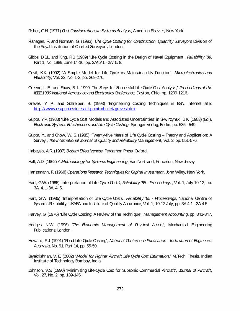
272
Fisher, G.H. (1971) Cost Considerations in Systems Analysis, American Elsevier, New York.
Flanagan, R. and Norman, G. (1983), Life Cycle Costing for Construction, Quantity Surveyors Division ofthe Royal Institution of Charted Surveyors, London.
Gibbs, D.J.L. and King, R.J. (1989) 'Life Cycle Costing in the Design of Naval Equipment', Reliability '89,Part 1, No. 1989, June 14-16, pp. 2A/5/1 - 2A/ 5/8.
Govil, K.K. (1992) 'A Simple Model for Life-Cycle vs Maintainability Function', Microelectronics andReliability, Vol. 32, No. 1-2, pp. 269-270.
Greene, L. E., and Shaw, B. L. 1990 ‘The Steps for Successful Life Cycle Cost Analysis,’ Proceedings of theIEEE 1990 National Aerospace and Electronics Conference, Dayton, Ohio, pp. 1209-1216.
Greves, Y. P., and Schreiber, B. (1993) ‘Engineering Costing Techniques in ESA, Internet site:http://www.esapub.esriu.esa.it.pointtobullet/greves.html.
Gupta, Y.P. (1983) ‘Life Cycle Cost Models and Associated Uncertainties’ in Skwirzynski, J. K. (1983) (Ed.),Electronic Systems Effectiveness and Life Cycle Costing, Springer-Verlag, Berlin, pp. 535 - 549.
Gupta, Y., and Chow, W. S. (1985) ‘Twenty-five Years of Life Cycle Costing – Theory and Application: ASurvey’, The International Journal of Quality and Reliability Management, Vol. 2, pp. 551-576.
Habayeb, A.R. (1987) System Effectiveness, Pergamon Press, Oxford.
Hall, A.D. (1962) A Methodology for Systems Engineering, Van Nostrand, Princeton, New Jersey.
Hanssmann, F. (1968) Operations Research Techniques for Capital Investment, John Wiley, New York.
Hart, G.W. (1985) 'Interpretation of Life Cycle Costs', Reliability '85 - Proceedings , Vol. 1, July 10-12, pp.3A. 4. 1-3A. 4. 5.
Hart, G.W. (1985) ‘Interpretation of Life Cycle Costs’, Reliability ’85 - Proceedings, National Centre ofSystems Reliability, UKAEA and Institute of Quality Assurance, Vol. 1, 10-12 July, pp. 3A.4.1 - 3A.4.5.
Harvey, G. (1976) ‘Life Cycle Costing: A Review of the Technique’, Management Accounting, pp. 343-347.
Hodges, N.W. (1996) 'The Economic Management of Physical Assets', Mechanical EngineeringPublications, London.
Howard, R.J. (1991) 'Road Life Cycle Costing', National Conference Publication - Institution of Engineers,Australia, No. 91, Part 14, pp. 55-59.
Jayakrishnan, V. E. (2002) ‘Model for Fighter Aircraft Life Cycle Cost Estimation,’ M.Tech. Thesis, IndianInstitute of Technology Bombay, India
Johnson, V.S. (1990) 'Minimizing Life-Cycle Cost for Subsonic Commercial Aircraft', Journal of Aircraft,Vol. 27, No. 2, pp. 139-145.
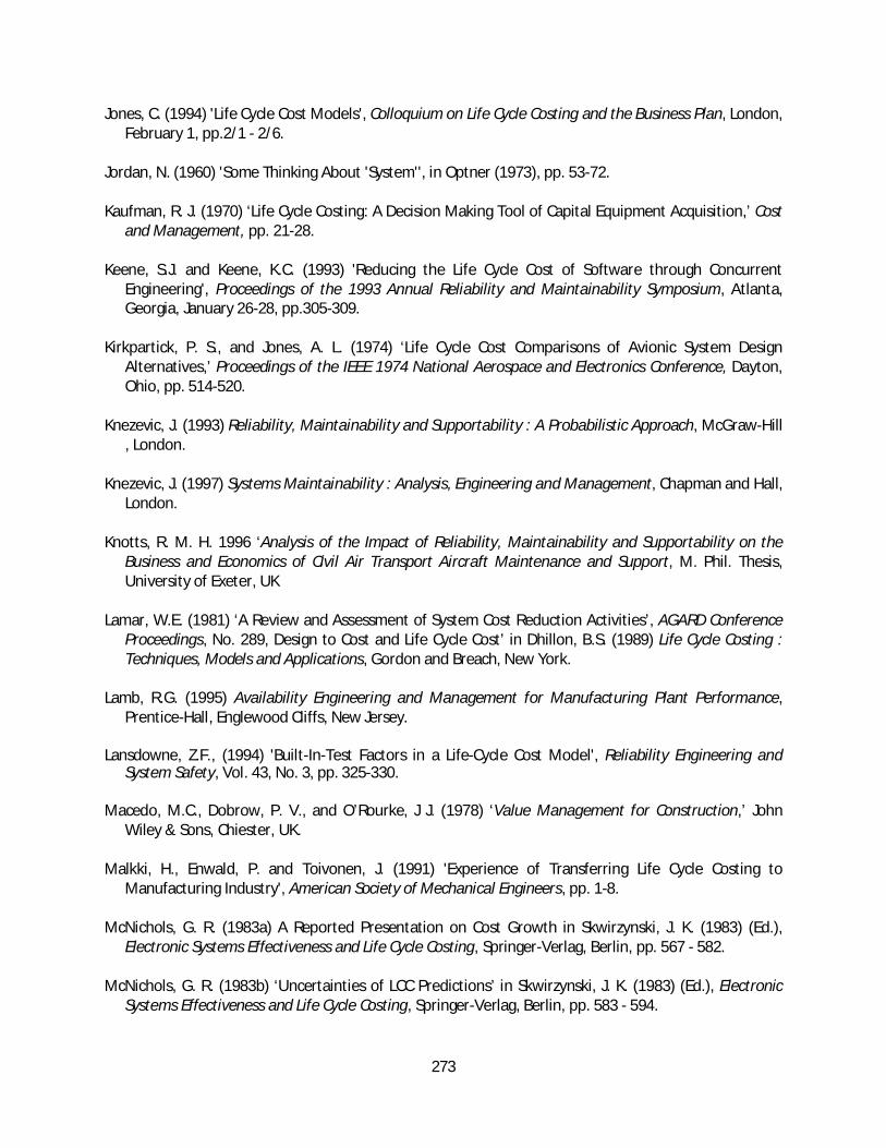
273
Jones, C. (1994) 'Life Cycle Cost Models', Colloquium on Life Cycle Costing and the Business Plan, London,February 1, pp.2/1 - 2/6.
Jordan, N. (1960) 'Some Thinking About 'System'', in Optner (1973), pp. 53-72.
Kaufman, R. J. (1970) ‘Life Cycle Costing: A Decision Making Tool of Capital Equipment Acquisition,’ Costand Management, pp. 21-28.
Keene, S.J. and Keene, K.C. (1993) 'Reducing the Life Cycle Cost of Software through ConcurrentEngineering', Proceedings of the 1993 Annual Reliability and Maintainability Symposium, Atlanta,Georgia, January 26-28, pp.305-309.
Kirkpartick, P. S., and Jones, A. L. (1974) ‘Life Cycle Cost Comparisons of Avionic System DesignAlternatives,’ Proceedings of the IEEE 1974 National Aerospace and Electronics Conference, Dayton,Ohio, pp. 514-520.
Knezevic, J. (1993) Reliability, Maintainability and Supportability : A Probabilistic Approach, McGraw-Hill, London.
Knezevic, J. (1997) Systems Maintainability : Analysis, Engineering and Management, Chapman and Hall,London.
Knotts, R. M. H. 1996 ‘Analysis of the Impact of Reliability, Maintainability and Supportability on theBusiness and Economics of Civil Air Transport Aircraft Maintenance and Support, M. Phil. Thesis,University of Exeter, UK
Lamar, W.E. (1981) ‘A Review and Assessment of System Cost Reduction Activities’, AGARD ConferenceProceedings, No. 289, Design to Cost and Life Cycle Cost’ in Dhillon, B.S. (1989) Life Cycle Costing :Techniques, Models and Applications, Gordon and Breach, New York.
Lamb, R.G. (1995) Availability Engineering and Management for Manufacturing Plant Performance,Prentice-Hall, Englewood Cliffs, New Jersey.
Lansdowne, Z.F., (1994) 'Built-In-Test Factors in a Life-Cycle Cost Model', Reliability Engineering andSystem Safety, Vol. 43, No. 3, pp. 325-330.
Macedo, M.C., Dobrow, P. V., and O’Rourke, J J. (1978) ‘Value Management for Construction,’ JohnWiley & Sons, Chiester, UK.
Malkki, H., Enwald, P. and Toivonen, J. (1991) 'Experience of Transferring Life Cycle Costing toManufacturing Industry', American Society of Mechanical Engineers, pp. 1-8.
McNichols, G. R. (1983a) A Reported Presentation on Cost Growth in Skwirzynski, J. K. (1983) (Ed.),Electronic Systems Effectiveness and Life Cycle Costing, Springer-Verlag, Berlin, pp. 567 - 582.
McNichols, G. R. (1983b) ‘Uncertainties of LCC Predictions’ in Skwirzynski, J. K. (1983) (Ed.), ElectronicSystems Effectiveness and Life Cycle Costing, Springer-Verlag, Berlin, pp. 583 - 594.
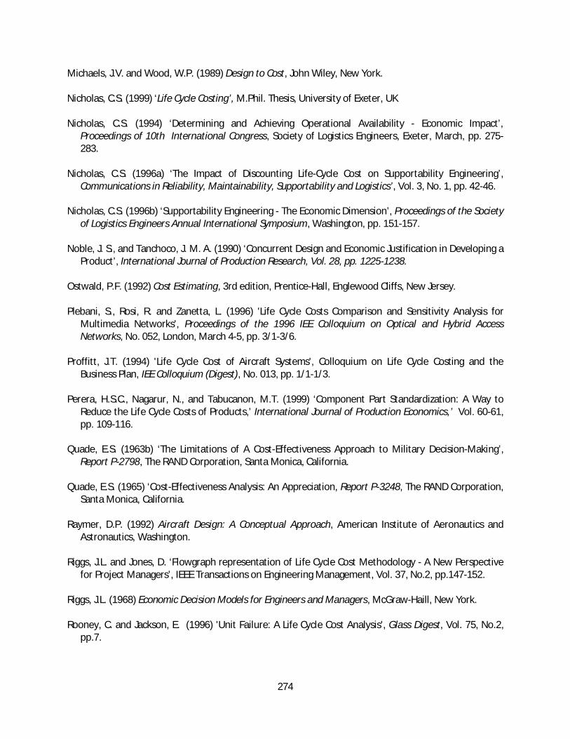
274
Michaels, J.V. and Wood, W.P. (1989) Design to Cost, John Wiley, New York.
Nicholas, C.S. (1999) ‘Life Cycle Costing’, M.Phil. Thesis, University of Exeter, UK
Nicholas, C.S. (1994) ‘Determining and Achieving Operational Availability - Economic Impact’,Proceedings of 10th International Congress, Society of Logistics Engineers, Exeter, March, pp. 275-283.
Nicholas, C.S. (1996a) ‘The Impact of Discounting Life-Cycle Cost on Supportability Engineering’,Communications in Reliability, Maintainability, Supportability and Logistics’, Vol. 3, No. 1, pp. 42-46.
Nicholas, C.S. (1996b) ‘Supportability Engineering - The Economic Dimension’, Proceedings of the Societyof Logistics Engineers Annual International Symposium, Washington, pp. 151-157.
Noble, J. S., and Tanchoco, J. M. A. (1990) ‘Concurrent Design and Economic Justification in Developing aProduct’, International Journal of Production Research, Vol. 28, pp. 1225-1238.
Ostwald, P.F. (1992) Cost Estimating, 3rd edition, Prentice-Hall, Englewood Cliffs, New Jersey.
Plebani, S., Rosi, R. and Zanetta, L. (1996) 'Life Cycle Costs Comparison and Sensitivity Analysis forMultimedia Networks', Proceedings of the 1996 IEE Colloquium on Optical and Hybrid AccessNetworks, No. 052, London, March 4-5, pp. 3/1-3/6.
Proffitt, J.T. (1994) 'Life Cycle Cost of Aircraft Systems', Colloquium on Life Cycle Costing and theBusiness Plan, IEE Colloquium (Digest), No. 013, pp. 1/1-1/3.
Perera, H.S.C., Nagarur, N., and Tabucanon, M.T. (1999) ‘Component Part Standardization: A Way toReduce the Life Cycle Costs of Products,’ International Journal of Production Economics,’ Vol. 60-61,pp. 109-116.
Quade, E.S. (1963b) ‘The Limitations of A Cost-Effectiveness Approach to Military Decision-Making’,Report P-2798, The RAND Corporation, Santa Monica, California.
Quade, E.S. (1965) ‘Cost-Effectiveness Analysis: An Appreciation, Report P-3248, The RAND Corporation,Santa Monica, California.
Raymer, D.P. (1992) Aircraft Design: A Conceptual Approach, American Institute of Aeronautics andAstronautics, Washington.
Riggs, J.L. and Jones, D. ‘Flowgraph representation of Life Cycle Cost Methodology - A New Perspectivefor Project Managers’, IEEE Transactions on Engineering Management, Vol. 37, No.2, pp.147-152.
Riggs, J.L. (1968) Economic Decision Models for Engineers and Managers, McGraw-Haill, New York.
Rooney, C. and Jackson, E. (1996) 'Unit Failure: A Life Cycle Cost Analysis', Glass Digest, Vol. 75, No.2,pp.7.
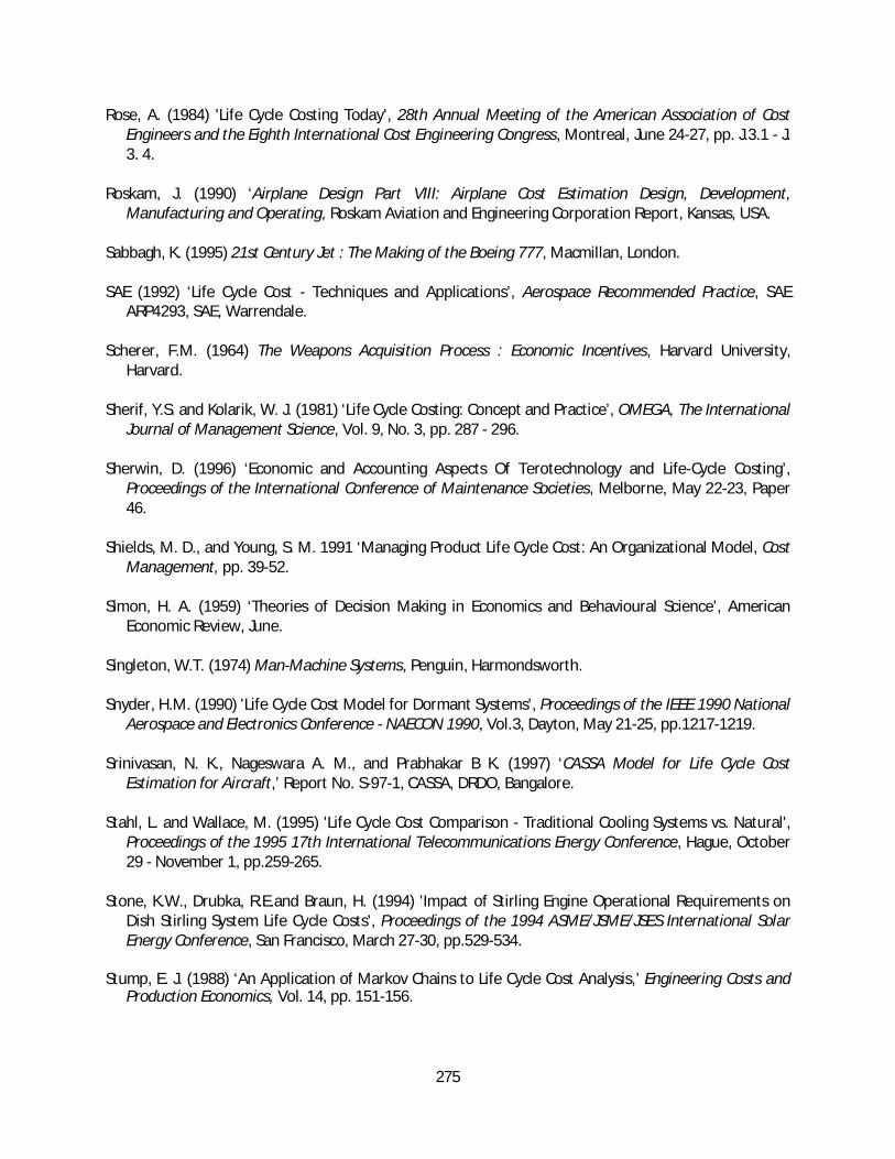
275
Rose, A. (1984) 'Life Cycle Costing Today', 28th Annual Meeting of the American Association of CostEngineers and the Eighth International Cost Engineering Congress, Montreal, June 24-27, pp. J.3.1 - J.3. 4.
Roskam, J. (1990) ‘Airplane Design Part VIII: Airplane Cost Estimation Design, Development,Manufacturing and Operating, Roskam Aviation and Engineering Corporation Report, Kansas, USA.
Sabbagh, K. (1995) 21st Century Jet : The Making of the Boeing 777, Macmillan, London.
SAE (1992) ‘Life Cycle Cost - Techniques and Applications’, Aerospace Recommended Practice, SAEARP4293, SAE, Warrendale.
Scherer, F.M. (1964) The Weapons Acquisition Process : Economic Incentives, Harvard University,Harvard.
Sherif, Y.S. and Kolarik, W. J. (1981) ‘Life Cycle Costing: Concept and Practice’, OMEGA, The InternationalJournal of Management Science, Vol. 9, No. 3, pp. 287 - 296.
Sherwin, D. (1996) ‘Economic and Accounting Aspects Of Terotechnology and Life-Cycle Costing’,Proceedings of the International Conference of Maintenance Societies, Melborne, May 22-23, Paper46.
Shields, M. D., and Young, S. M. 1991 ‘Managing Product Life Cycle Cost: An Organizational Model, CostManagement, pp. 39-52.
Simon, H. A. (1959) ‘Theories of Decision Making in Economics and Behavioural Science’, AmericanEconomic Review, June.
Singleton, W.T. (1974) Man-Machine Systems, Penguin, Harmondsworth.
Snyder, H.M. (1990) 'Life Cycle Cost Model for Dormant Systems', Proceedings of the IEEE 1990 NationalAerospace and Electronics Conference - NAECON 1990, Vol.3, Dayton, May 21-25, pp.1217-1219.
Srinivasan, N. K., Nageswara A. M., and Prabhakar B K. (1997) ‘CASSA Model for Life Cycle CostEstimation for Aircraft,’ Report No. S-97-1, CASSA, DRDO, Bangalore.
Stahl, L. and Wallace, M. (1995) 'Life Cycle Cost Comparison - Traditional Cooling Systems vs. Natural',Proceedings of the 1995 17th International Telecommunications Energy Conference, Hague, October29 - November 1, pp.259-265.
Stone, K.W., Drubka, R.E.and Braun, H. (1994) 'Impact of Stirling Engine Operational Requirements onDish Stirling System Life Cycle Costs', Proceedings of the 1994 ASME/JSME/JSES International SolarEnergy Conference, San Francisco, March 27-30, pp.529-534.
Stump, E. J. (1988) ‘An Application of Markov Chains to Life Cycle Cost Analysis,’ Engineering Costs andProduction Economics, Vol. 14, pp. 151-156.
276
Takagishi, S.K. (1989) 'Electric Power versus Petrol, Methanol or Gas. Life Cycle Cost Comparison', 9thInternational Electric Vehicle Symposium, Electric Vehicle Developments,Vol. 8, No. 3, Toronto,November 13-15, pp.77-81.
Taylor, W.B. (1981) ‘The Use of Life Cycle Costing in Acquiring Physical Assets’, Long Range Planning, Vol.14, pp. 32-43.
Thuesen, G.J. and Fabrycky, W.J. (1989) Engineering Economy, 7th edition, Prentice-Hall, EnglewoodCliffs, New Jersey.
UK Department of Industry (1977) ‘Life Cycle Costing in the Management of Assets', Department ofIndustry, Committee for Terotechnology, H.M.S.O., London.
US Department of Defense, (1983a) ‘Design to Cost’, Directive 4245.3, US Department of Defense.
US Department of Defense, (1983b) ‘Life Cycle Cost in Navy Acquisitions’, MIL-HDBK-259 (Navy), USDepartment of Defense.
US Department of Defense, (1996) ‘Major Systems Acquisitions’, Directive 5000.1 (Revised), USDepartment of Defense.
Vacek, R.M., Hopkins, M. and MacPherson, W.H. (1996) 'Development, Demonstration and Integrationof Advanced Technologies to Improve the Life Cycle Costs of Space Systems', Proceedings of the 1996IEEE Aerospace Applications Conference, Vol. 1, IEEE, Los Alamos, pp. 217-225.
Verma, D. (1995) ‘Conceptual System Design Synthesis, Analysis and Evaluation’, Technical Monograph1, Centre for Management of Industrial Reliability, Cost and Effectiveness, Faculty of Engineering,University of Exeter, Exeter.
Vivona, M.A. (1994) ‘Audit Environmental Processes Using Life-Cycle Costs’, Hydrocarbon Processing,Vol. 73, No. 8, p. 115.
White, G. E., and Ostwald, P. H. (1976) ‘Management Accounting’, pp. 39-42.
White, J.A., Agee, M.H. and Case, K.E. (1977) Principles of Engineering Economic Analysis, John Wiley,New York.
Wilkinson, V.K. (1990) 'Life Cycle Cost Analyses of Government Production and Services', Proceedings ofthe 1990 International Industrial Engineering Conference, No. 1990, San Francisco, May 20-23, pp.111-116.
Winkel, J.D. (1996) 'Use of Life Cycle Costing in New and Mature Applications', Proceedings of the 1996NPF/SPE European Production Operations Conference, Society of Petroleum Engineers (SPE),Stavanger, Norway, April 16-17, pp. 239-248.
Wonsiewicz, T.J. (1988) 'Life Cycle Cost Analysis. Key Assumptions and Sensitivity of Results',Transportation Research Record, Lane Enterprises Inc, Camp Hill, pp.113-117.
Woodward D. G. (1997) ‘Life Cycle Costing – Theory, Information, Acquisition and Application,’International Journal of Project Management, Vol. 15, No. 6, pp. 335-344.
277
Woud, J.K., Smit, K. and Vucinic, B. (1997) 'Maintenance Programme Design for Minimal Life Cycle Costsand Acceptable Safety Risks', International Shipbuilding Progress, Vol. 44, No. 437, Delft UniversityPress, Delft, Netherlands, pp.77-100.
Zhi, H. (1993) 'Simulation Analysis in Project Life Cycle Cost', Cost Engineering, Vol. 35, No. 12,Morgantown, West Virginia, pp. 13-17.
Zhou, X. and Cai, N. (1994) 'Dynamic Study of the Relationship between Life Cycle Cost and Reliability inElectronic Product', Tien Tzu Hsueh Pao/Acta Electronica Sinica, Vol. 22, No. 11, Hangzhou Inst. ofElectronics Engineering, Hangzhou, China, pp.22-27.
278
Total Cost of Ownership for Railway Assets: A Case Study on BOXN Wagons of Indian Railways
U Dinesh Kumar*, Gopinath Chattopadhyay** and H S Pannu***
*Indian Institute of Management Calcutta, Joka, D H Road, Kolkata 700104, INDIA
**Dept. of Mechanical, Manufacturing and Medical Engineering, Queensland University of Technology,Brisbane, QLD 4001, Australia
***South Eastern Railway, Garden Reach Road, Kolkata 700043, INDIA
[email protected], [email protected], [email protected]
ABSTRACT
Decision to purchase any capital equipment must be based on its total cost of ownership (TCO) ratherthan the usual practice of procurement based on the initial purchase price. In the recent years, TCO hasbecome a part of the strategic cost management and the concept can be applied for effectiveprocurement of railway assets. TCO provides an insight into the total cost of acquisition and sustenanceand thus effectively support decision-making in evaluation of various alternatives. The primaryobjective of this paper is to develop models for prediction of cost of ownership of capital assets. Themodels are developed using the Markov and renewal processes depending on the time to failuredistribution of individual items within the capital equipment. The models developed in this paper arevalidated using the data from BOXN wagon used by the Indian Railways.
Keywords: Asset management, Maintenance, Markov and renewal processes, Total cost of ownership.
1. INTRODUCTION
“Value for Money” has become one of the important criteria in an increasingly competitive businessenvironment. Life Cycle Cost (LCC) and the Total Cost of Ownership (TCO) are two important financialmeasures that are used for decision making in acquisitions to evaluate the value of any capitalequipment (Hampton, 2004; Humphries, 2004). Life cycle cost refers to all costs associated with the

279
product or system as applied to defined life cycle. That is, starting from requirement analysis, design,production, operation and maintenance till disposal. Total cost of ownership (TCO) is a philosophy,which is aimed at understanding the true cost of buying a particular product or service from a particularsupplier. From its origins in defence equipment procurement in the US in early 1960s, the use of lifecycle cost and cost of ownership has extended to other areas of the public and private sectors. LCC andTCO are being used to assist in decision-making, budget planning, cost control, and range of otheractivities that occur over the life of complex technological equipment.
LCC analysis is applied routinely to military projects (Blanchard, 1986). In the military sector theconsumer, by funding the project and operating the related product, essentially bears the total life cyclecost covering the major cost elements in all stages of a product’s life cycle. The term LCC analysis israrely used in the commercial sector. Instead, the main focus is on TCO where related costs, coveringacquisition (purchase or lease), operation, maintenance and support are borne by the customer. Inaddition, the customer can also incur costs when the product is not available for use, that is, ‘down timecosts’.
The objectives of LCC/TCO are (Flanagan and Norman, 1983):
• To enable investment options to be more effectively evaluated.• To consider the impact of all costs rather than only the initial capital costs.• To assist in the effective management of completed projects.• To facilitate choice between competing alternatives.
In the Defence industry the system’s life cycle is divided into various phases, which allow properplanning and control of a project. The number of phases depends on the nature of the project, purposeand whether they are applied to commercial, military or space projects (Knotts, 1998). Commonly usedphases are:
8. Requirements (Functional Specification).9. Concept/Feasibility Studies.10. Design and Development.11. Production.12. Testing and Certification.13. Operation, Maintenance and Support.14. Disposal
It is reported by the US Department of Defence that 70% of weapon system life cycle cost iscommitted by the end of concept studies, 85% by the end of system definition and 95% by the end offull scale development (Knotts, 1998). The US Department of Defence has formally used the concept oflife cycle cost in weapon system acquisition since the early 1960s through life cycle costing and life cyclecost analysis.
The cost of ownership approach identifies all future costs and reduces them to their presentvalue by use of the discounting techniques through which the economic worth of a product or product
280
options can be assessed. In order to achieve these objectives the following elements of cost ofownership have been identified (Woorward, 1997):
• Initial capital costs• Life of the asset• The discount rate• Operating and maintenance costs• Disposal cost
1.2 Initial capital costs
The initial capital costs can be divided into three sub-categories of cost namely: (1) purchase costs,(2) acquisition/finance costs, and (3) installation/commissioning/training costs. Purchase costs willinclude assessment of items such as land, buildings, fees, and equipment. Finance costs includealternative sources of funds. Basically, the initial capital cost category includes all the costs of buyingthe physical asset and bringing it into operation.
1. Life of the Asset
The estimated life of an asset has a major influence on life cycle cost analysis. Ferry et al (1991) hasdefined the following five possible determinants of an asset’s life expectancy:
• Functional life – the period over which the need for the asset is anticipated.
• Physical life – the period over which the asset may be expected to last physically, to when
replacement or major rehabilitation is physically required.
• Technological life – the period until technical obsolescence dictates replacement due to the
development of a technologically superior alternative.
• Economic life – the period until economic obsolescence dictates replacement with a lower
cost alternative.
• Social and legal life – the period until human desire or legal requirement dictates
replacement.
1.4 The discount rate
As the cost of ownership is discounted to their present value, selection of a suitable discount rate iscrucial for TCO analysis. A high discount rate will tend to favour options with low capital cost, short lifeand high recurring cost, whilst a low discount rate will have the opposite effect.
281
1.5 Operations and Maintenance Costs
Cost of ownership, in many cases, is about operation and maintenance cost. Estimation ofoperation and maintenance costs is the essential to minimise the total cost of ownership of the asset. Inthe whole of TCO analysis, estimation of operation and maintenance is the most challenging task.
1.6 Disposal cost
This is the cost incurred at the end of as asset’s working life in disposing of the asset. Thedisposal cost would include the cost of demolition, scrapping or selling the asset.
1.7 Uncertainties and Sensitivity Analysis
LCC/TCO is highly dependent on the assumptions and estimates made while collecting data.Even though it is possible to improve the quality of these estimates, there is always an element ofuncertainty associated with these estimates and assumptions. Macedo et al (1978) identifies thefollowing five major sources of uncertainty:
6. Differences between the actual and expected performance of the system could affect futureoperation and maintenance cost.
7. Changes in operational assumptions arising from modifications in user activity.8. Future technological advances that could provide lower cost alternatives and hence shorten the
economic life of any system/subsystem.9. Changes in the price levels of major resources such as energy or manpower, relative to other
resources can affect future alteration costs.10. Error in estimating relationships, price rates for specific resources and the rate of inflation in
overall costs from the time of estimation to the availability of the asset.
While undertaking a LCC/TCO analysis, there may be some key parameters about which uncertaintyexists, usually because of the inadequacy of the input data. Blanchard (1972) suggested the followingshould be the subject of sensitivity analysis:
1. Frequency of the maintenance factor.2. Variation of the asset’s utilization or operating time.3. Extent of the system’s self-diagnostic capability.4. Variation of corrective maintenance hours per operating hour.5. Product demand rate.6. The discount rate
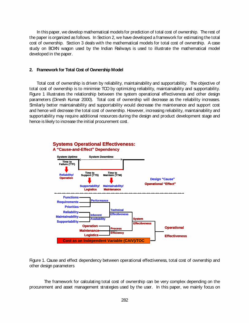
282
In this paper, we develop mathematical models for prediction of total cost of ownership. The rest ofthe paper is organized as follows. In Section 2, we have developed a framework for estimating the totalcost of ownership. Section 3 deals with the mathematical models for total cost of ownership. A casestudy on BOXN wagon used by the Indian Railways is used to illustrate the mathematical modeldeveloped in the paper.
2. Framework for Total Cost of Ownership Model
Total cost of ownership is driven by reliability, maintainability and supportability. The objective oftotal cost of ownership is to minimise TCO by optimizing reliability, maintainability and supportability.Figure 1 illustrates the relationship between the system operational effectiveness and other designparameters (Dinesh Kumar 2000). Total cost of ownership will decrease as the reliability increases.Similarly better maintainability and supportability would decrease the maintenance and support costand hence will decrease the total cost of ownership. However, increasing reliability, maintainability andsupportability may require additional resources during the design and product development stage andhence is likely to increase the initial procurement cost.
Figure 1. Cause and effect dependency between operational effectiveness, total cost of ownership andother design parameters
The framework for calculating total cost of ownership can be very complex depending on theprocurement and asset management strategies used by the user. In this paper, we mainly focus on
Systems Operational Effectiveness:Systems Operational Effectiveness:A CauseA Cause--andand--Effect DependencyEffect Dependency
Reliability/
Supportability/ Maintainability/
Design CauseOperational Effect
Operation
Logistics Maintenance
Time toSupport (TTS)
Time toMaintain (TTM)
Time toFailure (TTF)
System DowntimeSystem Uptime
SystemEffectiveness
OperationMaintenance
Logistics
ProcessEfficiency
OperationalOperational
EffectivenessEffectivenessCost as an Independent Variable (CAIV)/TOC
ReliabilityMaintainabilitySupportability
Availability
TechnicalEffectivenessInherent
PerformanceFunctions
RequirementsPriorities
Systems Operational Effectiveness:Systems Operational Effectiveness:A CauseA Cause--andand--Effect DependencyEffect Dependency
Reliability/
Supportability/ Maintainability/
Design CauseReliability/
Supportability/ Maintainability/
Design CauseOperational Effect
Operation
Logistics Maintenance
Operational Effect
Operation
Logistics Maintenance
Time toSupport (TTS)
Time toMaintain (TTM)
Time toFailure (TTF)
System DowntimeSystem Uptime
SystemEffectiveness
OperationMaintenance
Logistics
ProcessEfficiency
SystemEffectiveness
OperationMaintenance
Logistics
ProcessEfficiency
OperationalOperational
EffectivenessEffectivenessCost as an Independent Variable (CAIV)/TOC
OperationalOperational
EffectivenessEffectivenessCost as an Independent Variable (CAIV)/TOC
ReliabilityMaintainabilitySupportability
Availability
TechnicalEffectivenessInherent
ReliabilityMaintainabilitySupportability
Availability
TechnicalEffectivenessInherent
PerformanceFunctions
RequirementsPriorities
PerformanceFunctions
RequirementsPriorities

283
procurement, operation, maintenance and disposal cost, which are more relevant for assets likewagons. The framework shown in Figure 2 is used for evaluation of total cost of ownership.
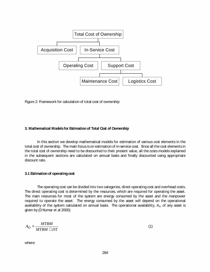
284
Figure 2: Framework for calculation of total cost of ownership
3. Mathematical Models for Estimation of Total Cost of Ownership
In this section we develop mathematical models for estimation of various cost elements in thetotal cost of ownership. The main focus is on estimation of in-service cost. Since all the cost elements inthe total cost of ownership need to be discounted to their present value, all the costs models explainedin the subsequent sections are calculated on annual basis and finally discounted using appropriatediscount rate.
3.1 Estimation of operating cost
The operating cost can be divided into two categories, direct operating cost and overhead costs.The direct operating cost is determined by the resources, which are required for operating the asset.The main resources for most of the system are energy consumed by the asset and the manpowerrequired to operate the asset. The energy consumed by the asset will depend on the operationalavailability of the system calculated on annual basis. The operational availability, Ao, of any asset isgiven by (D Kumar et al 2000):
DTMTBMMTBMAO +
= (1)
where:
Acquisition Cost
Operating Cost
Maintenance Cost Logistics Cost
Support Cost
In-Service Cost
Total Cost of Ownership
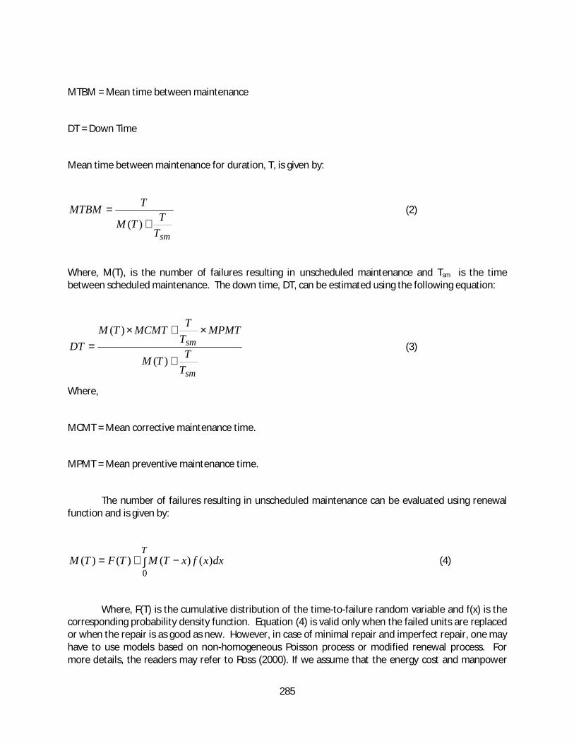
285
MTBM = Mean time between maintenance
DT = Down Time
Mean time between maintenance for duration, T, is given by:
smTTTM
TMTBM+
=)(
(2)
Where, M(T), is the number of failures resulting in unscheduled maintenance and Tsm is the timebetween scheduled maintenance. The down time, DT, can be estimated using the following equation:
sm
sm
TTTM
MPMTTTMCMTTM
DT+
×+×=
)(
)( (3)
Where,
MCMT = Mean corrective maintenance time.
MPMT = Mean preventive maintenance time.
The number of failures resulting in unscheduled maintenance can be evaluated using renewalfunction and is given by:
∫ −+=T
dxxfxTMTFTM0
)()()()( (4)
Where, F(T) is the cumulative distribution of the time-to-failure random variable and f(x) is thecorresponding probability density function. Equation (4) is valid only when the failed units are replacedor when the repair is as good as new. However, in case of minimal repair and imperfect repair, one mayhave to use models based on non-homogeneous Poisson process or modified renewal process. Formore details, the readers may refer to Ross (2000). If we assume that the energy cost and manpower
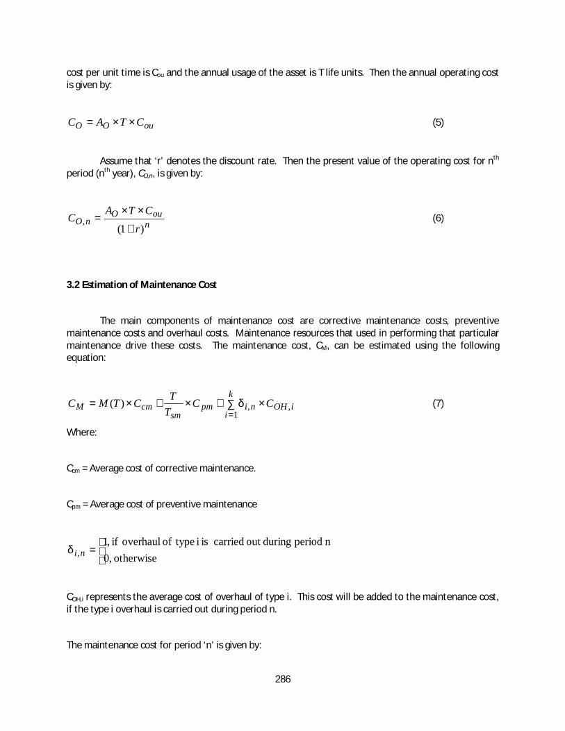
286
cost per unit time is Cou and the annual usage of the asset is T life units. Then the annual operating costis given by:
ouOO CTAC ××= (5)
Assume that ‘r’ denotes the discount rate. Then the present value of the operating cost for nth
period (nth year), CO,n, is given by:
nouO
nOr
CTAC)1(
,+
××= (6)
3.2 Estimation of Maintenance Cost
The main components of maintenance cost are corrective maintenance costs, preventivemaintenance costs and overhaul costs. Maintenance resources that used in performing that particularmaintenance drive these costs. The maintenance cost, CM, can be estimated using the followingequation:
∑ ×+×+×==
k
iiOHnipm
smcmM CC
TTCTMC
1,,)( δ (7)
Where:
Ccm = Average cost of corrective maintenance.
Cpm = Average cost of preventive maintenance
=otherwise,0
nperiodduringoutcarriedisi typeofoverhaulif,1,niδ
COH,i represents the average cost of overhaul of type i. This cost will be added to the maintenance cost,if the type i overhaul is carried out during period n.
The maintenance cost for period ‘n’ is given by:
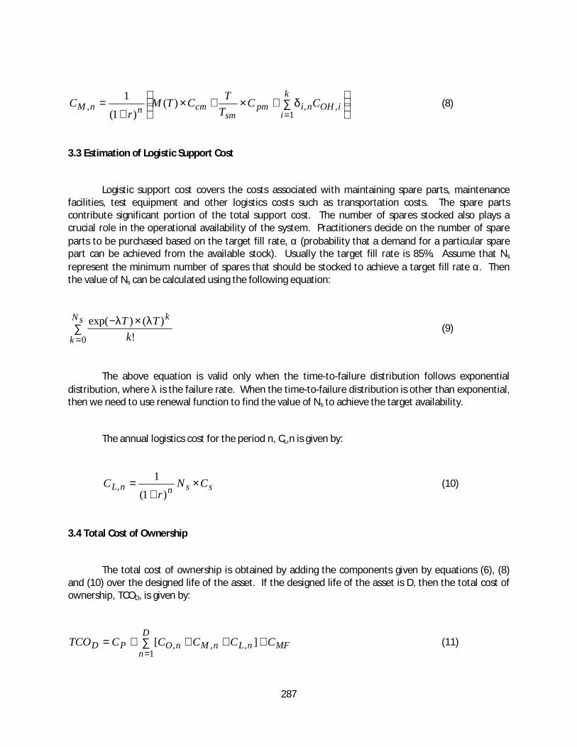
287
∑+×+×
+=
=iOH
k
inipm
smcmnnM CC
TTCTM
rC ,
1,, )(
)1(1
δ (8)
3.3 Estimation of Logistic Support Cost
Logistic support cost covers the costs associated with maintaining spare parts, maintenancefacilities, test equipment and other logistics costs such as transportation costs. The spare partscontribute significant portion of the total support cost. The number of spares stocked also plays acrucial role in the operational availability of the system. Practitioners decide on the number of spareparts to be purchased based on the target fill rate, α (probability that a demand for a particular sparepart can be achieved from the available stock). Usually the target fill rate is 85%. Assume that Ns
represent the minimum number of spares that should be stocked to achieve a target fill rate α. Thenthe value of Ns can be calculated using the following equation:
∑×−
=
sN
k
k
kTT
0 !)()exp( λλ
(9)
The above equation is valid only when the time-to-failure distribution follows exponentialdistribution, where λ is the failure rate. When the time-to-failure distribution is other than exponential,then we need to use renewal function to find the value of Ns to achieve the target availability.
The annual logistics cost for the period n, CL,n is given by:
ssnnL CNr
C ×+
=)1(
1, (10)
3.4 Total Cost of Ownership
The total cost of ownership is obtained by adding the components given by equations (6), (8)and (10) over the designed life of the asset. If the designed life of the asset is D, then the total cost ofownership, TCOD, is given by:
MFnLD
nnMnOPD CCCCCTCO ++∑ ++=
=][ ,
1,, (11)

288
Where CP is the procurement price of wagon and CMF is the one-time expenses of maintenanceand support equipment.
4. Case Study on BOXN wagons used by the Indian Railways
Indian railways are the principal mode of transport for raw material for steel plants, finished steelfrom steel plants, coal, iron, oil, cement, petroleum products, fertilizer and food grains in India. Indianrailways owns more than 5,00,000 wagons. The wagons have a design life of 35 years. The requirementof wagons for future is assessed on the basis of freight traffic projected and the anticipated level ofproductivity of wagons measured in terms of net ton kilometers (NTKM) per wagon per day likely to beachieved. The wagons are procured from the wagons India limited, which was incorporated in 1974.Wagons India limited supplies about 90% of the wagon requirement and the rest are purchased fromthe open market. The total cost of ownership is an important issue during the procurement of wagons.The procurement cost of wagon is $40,000.
The BOXN wagons are mainly used for carrying coal and are fitted with CASNUB bogies. CASNUBbogies are the critical subsystem of the wagon. The CASNUB bogie consists of two cast side frames anda floating bolster. The bolster is supported on the side frames through two groups of spring, which alsoincorporate the load proportional friction damping. The side frames of the CASNUB bogie areconnected by a fabricated mild steel spring plank to maintain the bogie square. The salient featuresCASNUB bogies are shown in Table 1.
Table 1. Salient features of CASNUB bogie
59.1.1.1 Gauge1676mm
Axle load 20.3t. However all bogies except Casnub 22HS can beupgraded upto 22.9t
Wheel Diameter 1000 mm (New). 956 mm ((New) for retrofittedCasnub 22W
Wheel Base 2000mmType of Axle Casnub- 22W (M)Bearing (a) Cylindrical roller bearing axle box in limited no. on
Casnub 22W Bogies only.(b) Standard AAR tapered cartridge bearing class ‘E’
suitable for 152.4x276.4mm (6”x11”) narrow jaw.
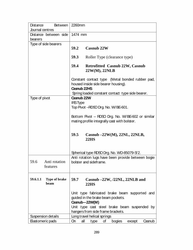
289
Distance BetweenJournal centres
2260mm
Distance between sidebearers
1474 mm
Type of side bearers59.2 Casnub 22W
59.3 Roller Type (clearance type)
59.4 Retrofitted Casnub 22W, Casnub22W(M), 22NLB
Constant contact type (Metal bonded rubber pad,housed inside side bearer housing).Casnub 22HS Spring loaded constant contact type side bearer.
Type of pivot Casnub 22WIRS TypeTop Pivot –RDSO Drg. No. W/BE-601.
Bottom Pivot – RDSO Drg. No. W/BE-602 or similarmating profile integrally cast with bolster.
59.5 Casnub 22W(M), 22NL, 22NLB,22HS
Spherical type RDSO Drg. No. WD-85079-S/2.
59.6 Anti rotationfeatures
Anti rotation lugs have been provide between bogiebolster and sideframe.
59.6.1.1 Type of brakebeam
59.7 Casnub 22W, /22NL, 22NLB and22HS
Unit type fabricated brake beam supported andguided in the brake beam pockets.Casnub 22W(M)Unit type cast steel brake beam suspended byhangers from side frame brackets.
Suspension details Long travel helical springsElastomeric pads On all type of bogies except Casnub
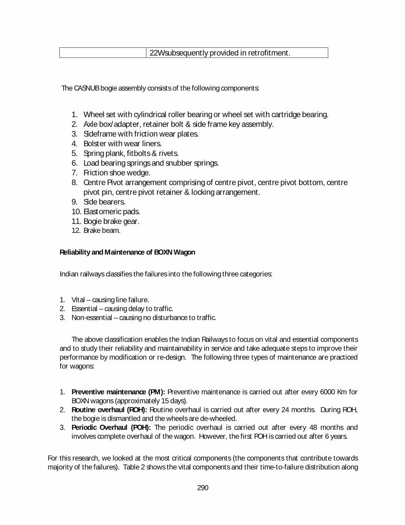
290
22Wsubsequently provided in retrofitment.
The CASNUB bogie assembly consists of the following components:
1. Wheel set with cylindrical roller bearing or wheel set with cartridge bearing.2. Axle box/adapter, retainer bolt & side frame key assembly.3. Sideframe with friction wear plates.4. Bolster with wear liners.5. Spring plank, fitbolts & rivets.6. Load bearing springs and snubber springs.7. Friction shoe wedge.8. Centre Pivot arrangement comprising of centre pivot, centre pivot bottom, centre
pivot pin, centre pivot retainer & locking arrangement.9. Side bearers.10. Elastomeric pads.11. Bogie brake gear.12. Brake beam.
Reliability and Maintenance of BOXN Wagon
Indian railways classifies the failures into the following three categories:
1. Vital – causing line failure.2. Essential – causing delay to traffic.3. Non-essential – causing no disturbance to traffic.
The above classification enables the Indian Railways to focus on vital and essential componentsand to study their reliability and maintainability in service and take adequate steps to improve theirperformance by modification or re-design. The following three types of maintenance are practicedfor wagons:
1. Preventive maintenance (PM): Preventive maintenance is carried out after every 6000 Km forBOXN wagons (approximately 15 days).
2. Routine overhaul (ROH): Routine overhaul is carried out after every 24 months. During ROH,the bogie is dismantled and the wheels are de-wheeled.
3. Periodic Overhaul (POH): The periodic overhaul is carried out after every 48 months andinvolves complete overhaul of the wagon. However, the first POH is carried out after 6 years.
For this research, we looked at the most critical components (the components that contribute towardsmajority of the failures). Table 2 shows the vital components and their time-to-failure distribution along
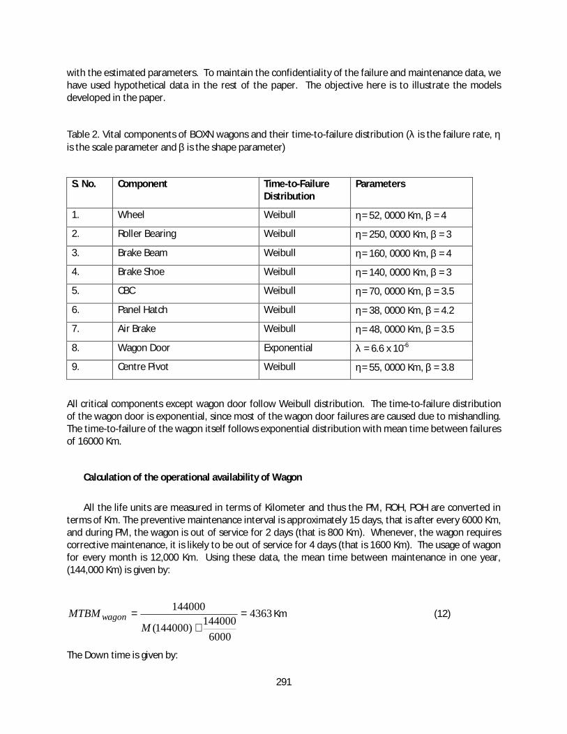
291
with the estimated parameters. To maintain the confidentiality of the failure and maintenance data, wehave used hypothetical data in the rest of the paper. The objective here is to illustrate the modelsdeveloped in the paper.
Table 2. Vital components of BOXN wagons and their time-to-failure distribution (λ is the failure rate, ηis the scale parameter and β is the shape parameter)
S. No. Component Time-to-FailureDistribution
Parameters
1. Wheel Weibull η= 52, 0000 Km, β = 4
2. Roller Bearing Weibull η= 250, 0000 Km, β = 3
3. Brake Beam Weibull η= 160, 0000 Km, β = 4
4. Brake Shoe Weibull η= 140, 0000 Km, β = 3
5. CBC Weibull η= 70, 0000 Km, β = 3.5
6. Panel Hatch Weibull η= 38, 0000 Km, β = 4.2
7. Air Brake Weibull η= 48, 0000 Km, β = 3.5
8. Wagon Door Exponential λ = 6.6 x 10⁻⁶
9. Centre Pivot Weibull η= 55, 0000 Km, β = 3.8
All critical components except wagon door follow Weibull distribution. The time-to-failure distributionof the wagon door is exponential, since most of the wagon door failures are caused due to mishandling.The time-to-failure of the wagon itself follows exponential distribution with mean time between failuresof 16000 Km.
Calculation of the operational availability of Wagon
All the life units are measured in terms of Kilometer and thus the PM, ROH, POH are converted interms of Km. The preventive maintenance interval is approximately 15 days, that is after every 6000 Km,and during PM, the wagon is out of service for 2 days (that is 800 Km). Whenever, the wagon requirescorrective maintenance, it is likely to be out of service for 4 days (that is 1600 Km). The usage of wagonfor every month is 12,000 Km. Using these data, the mean time between maintenance in one year,(144,000 Km) is given by:
4363
6000144000)144000(
144000=
+=
MMTBM wagon Km (12)
The Down time is given by:
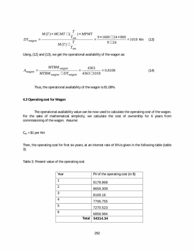
292
1018249
8002416009
)(
)()(=
+×+×
=+
×+×=
sm
smwagon
TTTM
MPMTTTMCMTTM
DT Km (13)
Using, (12) and (13), we get the operational availability of the wagon as:
8108.010184363
4363=
+=
+=
wagonwagon
wagonwagon DTMTBM
MTBMA (14)
Thus, the operational availability of the wagon is 81.08%.
4.3 Operating cost for Wagon
The operational availability value can be now used to calculate the operating cost of the wagon.For the sake of mathematical simplicity, we calculate the cost of ownership for 6 years fromcommissioning of the wagon. Assume:
Cou = $1 per Km
Then, the operating cost for first six years, at an interest rate of 6% is given in the following table (table3):
Table 3: Present value of the operating cost
Year PV of the operating cost (in $)
1 9178.8682 8659.3093 8169.164 7706.7555 7270.5236 6858.984
Total 54314.34
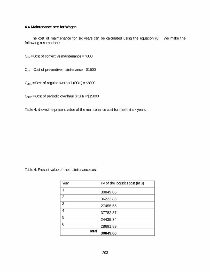
293
4.4 Maintenance cost for Wagon
The cost of maintenance for six years can be calculated using the equation (8). We make thefollowing assumptions:
Ccm = Cost of corrective maintenance = $800
Cpm = Cost of preventive maintenance = $1500
COH,1 = Cost of regular overhaul (ROH) = $8000
COH,2 = Cost of periodic overhaul (POH) = $15000
Table 4, shows the present value of the maintenance cost for the first six years.
Table 4: Present value of the maintenance cost
Year PV of the logistics cost (in $)
1 30849.062 36222.863 27455.554 37782.875 24435.346 28691.89
Total 30849.06
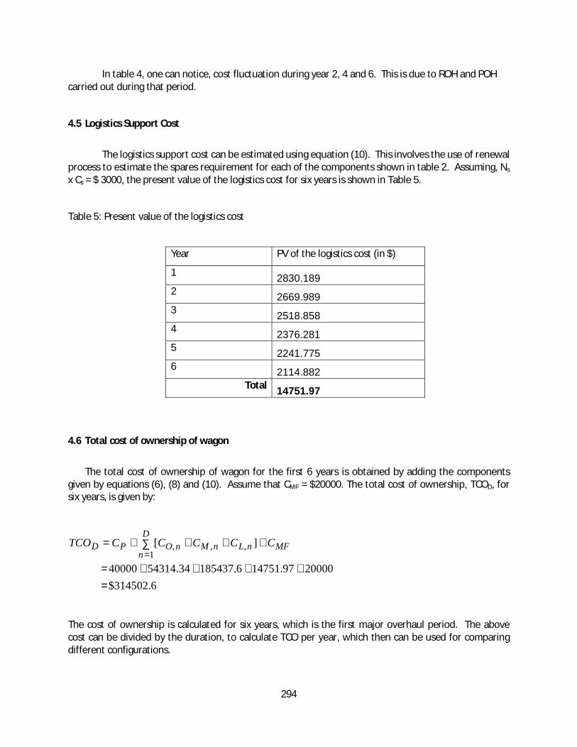
294
In table 4, one can notice, cost fluctuation during year 2, 4 and 6. This is due to ROH and POHcarried out during that period.
4.5 Logistics Support Cost
The logistics support cost can be estimated using equation (10). This involves the use of renewalprocess to estimate the spares requirement for each of the components shown in table 2. Assuming, Ns
x Cs = $ 3000, the present value of the logistics cost for six years is shown in Table 5.
Table 5: Present value of the logistics cost
Year PV of the logistics cost (in $)
1 2830.1892 2669.9893 2518.8584 2376.2815 2241.7756 2114.882
Total 14751.97
4.6 Total cost of ownership of wagon
The total cost of ownership of wagon for the first 6 years is obtained by adding the componentsgiven by equations (6), (8) and (10). Assume that CMF = $20000. The total cost of ownership, TCOD, forsix years, is given by:
6.314502$2000097.147516.18543734.5431440000
][ ,1
,,
=++++=
++∑ ++==
MFnLD
nnMnOPD CCCCCTCO
The cost of ownership is calculated for six years, which is the first major overhaul period. The abovecost can be divided by the duration, to calculate TCO per year, which then can be used for comparingdifferent configurations.
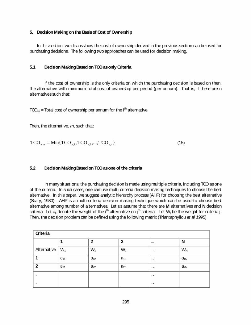
295
5. Decision Making on the Basis of Cost of Ownership
In this section, we discuss how the cost of ownership derived in the previous section can be used forpurchasing decisions. The following two approaches can be used for decision making.
5.1 Decision Making Based on TCO as only Criteria
If the cost of ownership is the only criteria on which the purchasing decision is based on then,the alternative with minimum total cost of ownership per period (per annum). That is, if there are nalternatives such that:
TCOa,i = Total cost of ownership per annum for the ith alternative.
Then, the alternative, m, such that:
}TCO,...,TCO,Min{TCOTCO na,a,2a,1ma, = (15)
5.2 Decision Making Based on TCO as one of the criteria
In many situations, the purchasing decision is made using multiple criteria, including TCO as oneof the criteria. In such cases, one can use multi criteria decision making techniques to choose the bestalternative. In this paper, we suggest analytic hierarchy process (AHP) for choosing the best alternative(Saaty, 1980). AHP is a multi-criteria decision making technique which can be used to choose bestalternative among number of alternatives. Let us assume that there are M alternatives and N decisioncriteria. Let aij denote the weight of the ith alternative on jth criteria. Let Wj be the weight for criteria j.Then, the decision problem can be defined using the following matrix (Triantaphyllou et al 1995)
Criteria
Alternative
1 2 3 N
W1 W2 W3 … WN
1 a11 a12 a13 … a1N
2 a21 a22 a23 … a2N
.
.
…
…
296
. …
M aM1 aM2 aM3 aMN
Using the above data AHP finds the overall importance of the alternative and chooses the one withmaximum weight (interested reader may refer to Saaty, 1980).
6. Conclusions
The main objectives of this paper are to develop framework for estimation of cost of ownership ofcapital assets and to develop mathematical models for estimation of various cost elements within thecost of ownership. The innovative approach used in this paper is the use of operational availability toestimate the operating cost. Most of the model use calendar time to estimate the operating time. Theuse of calendar time may be appropriate for certain elements of operating cost such as labor costs, thevariable costs such as energy consumed would depend on the operational availability of the system. Themodels developed in the paper are used illustrated using the wagons used in the Indian railways.Although, the data used in the paper are modified, it captures the impact of cost of ownership. In theexample, we have shown that the cost of ownership of wagon for six years is almost 8 times its initialprocurement price. The main aim of this paper is to show the significance and total cost of ownershipcompared to the procurement price and thus to prove that all procurement decisions must be based ontotal cost of ownership and not on the basis of procurement cost.
References
Anon. (2002), Procurement of wagons by Indian Railways, Report Number 9A, Indian Railways.
Blanchard, B. S. (1986), Logistics Engineering and Management, 3rd Edition, Prentice Hall, New Jersey.
Blanchard, B. S. (1988), Systems Engineering and Management, 2nd Edition, John Wiley, New York.
Blanchard, B. S. and Fabrycky, W. J. (1990), Systems Engineering and Analysis, 2nd Edition, Prentice Hall,New Jersey.
Dinesh Kumar, U., Crocker, J, Knezevic, J and El-Haram. (2000), Reliability, Maintenance and LogisticsSupport – A Life Cycle Approach, Kluwer Academic Publishers, Boston.
Hampton, T. (2004), The Cost of Ownership, ENR: Engineering News Record, Vol. 253, 7, 24-29.
Harvey, G. (1976), Life Cycle Costing: A Review of the Technique, Management Accounting, 343-347.
Humphries, J. (2004), Optimizing Total Cost of Ownership, Plant Engineers, Vol. 58, 7, 23-27.
Ross, S. (2000), Introduction to Probability Models, Academic Press, New York.
297
Saaty, T. L. (1980), The Analytic Hierarchy Process: Planning, Priority Setting and Resource Allocation,McGraw Hill.
Sherif, Y. S., and Kolarik, W. J. (1981), Life Cycle Costing: Concept and Practice, OMEGA, 9,.3, 287-296.
Taylor, W.B. (1981), The Use of Life Cycle Costing in Acquiring Physical Asset, Long Range Planning, 14,32-43.
Triantaphyllou, E., and Mann, S. (1995), Using Analytical Hierarchy Process in Decision Making inEngineering Applications: Some Challenges, International Journal of Industrial Engineering:Applications and Practice, Vol. 2, No. 1, 35-44