Embed Size (px)
DESCRIPTION
Álgebra Lineal Para Matemáticos, Físicos e Ingenieros
Citation preview
Undergraduate Texts in Mathematics
Serge Lang
Linear Algebra Third Edition
Springer
Springer New York Berlin Heidelberg Hong Kong London Milan Paris Tokyo
Undergraduate Texts in Mathematics
Editors
s. Axler
F. W. Gehring
K. A. Ribet
BOOKS OF RELATED INTEREST BY SERGE LANG
Math! Encounters with High School Students 1995, ISBN 0-387-96129-1
Geometry: A High School Course (with Gene Morrow) 1988, ISBN 0-387-96654-4
The Beauty of Doing Mathematics 1994, ISBN 0-387-96149-6
Basic Mathematics 1995, ISBN 0-387-96787-7
A First Course in Calculus, Fifth Edition 1993, ISBN 0-387-96201-8
Short Calculus 2002, ISBN 0-387-95327-2
Calculus of Several Variables, Third Edition 1987, ISBN 0-387-96405-3
Introduction to Linear Algebra, Second Edition 1997, ISBN 0-387-96205-0
Undergraduate Algebra, Second Edition 1994, ISBN 0-387-97279-X
Math Talks for Undergraduates 1999, ISBN 0-387-98749-5
Undergraduate Analysis, Second Edition 1996, ISBN 0-387-94841-4
Complex Analysis, Fourth Edition 1998, ISBN 0-387-98592-1
Real and Functional Analysis, Third Edition 1993, ISBN 0-387-94001-4
Algebraic Number Theory, Second Edition 1996, ISBN 0-387-94225-4
Introduction to Differentiable Manifolds, Second Edition 2002, ISBN 0-387-95477-5
Challenges 1998, ISBN 0-387-94861-9
Serge Lang
Linear Alge bra
Third Edition
With 21 Illustrations
Springer
Serge Lang Department of Mathematics Yale University New Haven, CT 06520 USA
Editorial Board
S. Axler Mathematics Department San Francisco State
University San Francisco, CA 94132 USA
F.W. Gehring Mathematics Department East Hall University of Michigan Ann Arbor, MI 48109 USA
Mathematics Subject Classification (2000): IS-0 1
Library of Congress Cataloging-in-Publication Data Lang, Serge
Linear algebra. (Undergraduate texts in mathematics) Includes bibliographical references and index. I. Algebras, Linear. II. Title. III. Series.
QA2Sl. L.26 1987 SI2'.S 86-21943
K.A. Ribet Mathematics Department University of California,
at Berkeley Berkeley, CA 94720-3840 USA
ISBN 0-387 -96412-6 Printed on acid-free paper.
The first edition of this book appeared under the title Introduction to Linear Algebra © 1970 by Addison-Wesley, Reading, MA. The second edition appeared under the title Linear Algebra © 1971 by Addison-Wesley, Reading, MA.
© 1987 Springer-Verlag New York, Inc. All rights reserved. This work may not be translated or copied in whole or in part without the written permission of the publisher (Springer-Verlag New York, Inc., 17S Fifth Avenue, New York, NY 10010, USA), except for brief excerpts in connection with reviews or scholarly analysis. Use In
connection with any form of information storage and retrieval, electronic adaptation, computer software, or by similar or dissimilar methodology now known or hereafter developed is forbidden. The use in this publication of trade names, trademarks, service marks, and similar terms, even if they are not identified as such, is not to be taken as an expression of opinion as to whether or not they are subject to proprietary rights.
Printed in the United States of America.
19 18 17 16 IS 14 13 12 11 (Corrected printing, 2004) SPIN 10972434
Springer-Verlag is part of Springer Science+Business Media
springeronline. com
Foreword
The present book is meant as a text for a course in linear algebra, at the undergraduate level in the upper division.
My Introduction to Linear Algebra provides a text for beginning students, at the same level as introductory calculus courses. The present book is meant to serve at the next level, essentially for a second course in linear algebra, where the emphasis is on the various structure theorems: eigenvalues and eigenvectors (which at best could occur only rapidly at the end of the introductory course); symmetric, hermitian and unitary operators, as well as their spectral theorem (diagonalization); triangulation of matrices and linear maps; Jordan canonical form; convex sets and the Krein-Milman theorem. One chapter also provides a complete theory of the basic properties of determinants. Only a partial treatment could be given in the introductory text. Of course, some parts of this chapter can still be omitted in a given course.
The chapter of convex sets is included because it contains basic results of linear algebra used in many applications and "geometric" linear algebra. Because logically it uses results from elementary analysis (like a continuous function on a closed bounded set has a maximum) I put it at the end. If such results are known to a class, the chapter can be covered much earlier, for instance after knowing the definition of a linear map.
I hope that the present book can be used for a one-term course. The first six chapters review some of the basic notions. I looked for efficiency. Thus the theorem that m homogeneous linear equations in n unknowns has a non-trivial soluton if n > m is deduced from the dimension theorem rather than the other way around as in the introductory text. And the proof that two bases have the same number of elements (i.e. that dimension is defined) is done rapidly by the "interchange"
VI FOREWORD
method. I have also omitted a discussion of elementary matrices, and Gauss elimination, which are thoroughly covered in my Introduction to Linear Algebra. Hence the first part of the present book is not a substitute for the introductory text. It is only meant to make the present book self contained, with a relatively quick treatment of the more basic material, and with the emphasis on the more advanced chapters. Today's curriculum is set up in such a way that most students, if not all, will have taken an introductory one-term course whose emphasis is on matrix manipulation. Hence a second course must be directed toward the structure theorems.
Appendix 1 gives the definition and basic properties of the complex numbers. This includes the algebraic closure. The proof of course must take for granted some elementary facts of analysis, but no theory of complex variables is used.
Appendix 2 treats the Iwasawa decomposition, in a topic where the group theoretic aspects begin to intermingle seriously with the purely linear algebra aspects. This appendix could (should?) also be treated in the general undergraduate algebra course.
Although from the start I take vector spaces over fields which are subfields of the complex numbers, this is done for convenience, and to avoid drawn out foundations. Instructors can emphasize as they wish that only the basic properties of addition, multiplication, and division are used throughout, with the important exception, of course, of those theories which depend on a positive definite scalar product. In such cases, the real and complex numbers play an essential role.
New Haven, Connecticut
Acknowledgments
SERGE LANG
I thank Ron Infante and Peter Pappas for assisting with the proof reading and for useful suggestions and corrections. I also thank Gimli Khazad for his corrections.
S.L.
Contents
CHAPTER I
Vector Spaces
§1. Definitions .. §2. Bases. . .. . .... §3. Dimension of a Vector Space . §4. Sums and Direct Sums . . . . .
CHAPTER II
Matrices . .
§1. The Space of Matrices ..... §2. Linear Equations. . . . §3. Multiplication of Matrices .
CHAPTER III
Linear Mappings .
§ 1. Mappings . . . §2. Linear Mappings. . §3. The Kernel and Image of a Linear Map §4. Composition and Inverse of Linear Mappings . . §5. Geometric Applications. . . . . . . . . . . . . . . .
CHAPTER IV
Linear Maps and Matrices. . . . . . . . . . . . .
§1. The Linear Map Associated with a Matrix. . §2. The Matrix Associated with a Linear Map. §3. Bases, Matrices, and Linear Maps . . . . . . .
1
2 10 15 19
23
23 29 31
43
43 51 59 66 72
81
81 82 87
Vl11 CONTENTS
CHAPTER V
Scalar Products and Orthogonality.
§ 1. Scalar Products. . . . . . . . . . . §2. §3. §4. §5. §6. §7. §8.
Orthogonal Bases, Positive Definite Case .. Application to Linear Equations; the Rank .. Bilinear Maps and Matrices . . . . . . General Orthogonal Bases ....... . The Dual Space and Scalar Products Quadratic Forms .............. . Sylvester's Theorem . . . . . . . . . . . .
CHAPTER VI
Determinants
§1. Determinants of Order 2 .. §2. §3. §4. §5. §6. §7. §8. §9.
Existence of Determinants Additional Properties of Determinants. Cramer's Rule . . . . . . . . . . . . . . . . Triangulation of a Matrix by Column Operations Permutations . . . . . . . . . . . . . . . . . . . . . . . Expansion Formula and Uniqueness of Determinants Inverse of a Matrix . . . . . . . . . . . . . . . . . The Rank of a Matrix and Subdeterminants . . . . ..
CHAPTER VII
- Symmetric, Hermitian, and Unitary Operators. .
§1. Symmetric Operators §2. Hermitian Operators §3. Unitary Operators . .
CHAPTER VIII
Eigenvectors and Eigenvalues
§1. Eigenvectors and Eigenvalues . §2. The Characteristic Polynomial. . §3. Eigenvalues and Eigenvectors of Symmetric Matrices §4. Diagonalization of a Symmetric Linear Map. . §5. The Hermitian Case. . . . . . . . . . . . §6. Unitary Operators . . . . . . . . . . . . . . . . .
CHAPTER IX
Polynomials and Matrices .
§1. Polynomials. . . . . . . . . . . . . . . . . . . . §2. Polynomials of Matrices and Linear Maps . .
.....
95
95 103 113 118 123 125 132 135
140
140 143 150 157 161 163 168 174 177
180
180 184 188
194
194 200 213 218 225 227
231
231 233
CONTENTS
CHAPTER X
Triangulation of Matrices and Linear Maps
§1. Existence of Triangulation . . . . . . §2. Theorem of Hamilton-Cayley ... §3. Diagonalization of Unitary Maps.
CHAPTER XI
Polynomials and Primary Decomposition. .
§1. The Euclidean Algorithm .. §2. Greatest Common Divisor . . . . . . . . . . . . . . §3. Unique Factorization ........... . §4. Application to the Decomposition of a Vector Space. §5. Schur's Lemma. . . . . . . . §6. The Jordan Normal Form ................ .
CHAPTER XII
Convex Sets
§ 1. Definitions ....... . §2. Separating Hyperplanes. §3. Extreme Points and Supporting Hyperplanes §4. The Krein-Milman Theorem .......... .
APPENDIX I
IX
237 237 240 242
245
245 248 251 255 260 262
268
268 270 272 274
Complex Numbers............................ . . . . . . . . . . . . . . . . . . . . . . . . . . . . . 277
APPENDIX II
Iwasawa Decomposition and Others . . . . . . . . . . . . . . . . . . . . . . . . . . . . . . . . . . . . . . . 283
Index..................................................................... 293

CHAPTER
Vector Spaces
As usual, a collection of objects will be called a set. A member of the collection is also called an element of the set. I t is useful in practice to use short symbols to denote certain sets. For instance, we denote by R the set of all real numbers, and by C the set of all complex numbers. To say that" x is a real number" or that" x is an element of R" amounts to the same thing. The set of all n-tuples of real numbers will be denoted by Rn. Thus "X is an element of Rn" and "X is an n-tuple of real numbers" mean the same thing. A review of the definition of C and its properties is given an Appendix.
Instead of saying that u is an element of a set S, we shall also frequently say that u lies in S and write u E S. If Sand S' are sets, and if every element of S' is an element of S, then we say that S' is a subset of S. Thus the set of real numbers is a subset of the set of complex numbers. To say that S' is a subset of S is to say that S' is part of S. Observe that our definition of a subset does not exclude the possibility that S' = S. If S' is a subset of S, but S' =1= S, then we shall say that S' is a proper subset of S. Thus C is a subset of C, but R is a proper subset of C. To denote the fact that S' is a subset of S, we write S' c S, and also say that S' is contained in S.
If Sl' S2 are sets, then the intersection of Sl and S2' denoted by Sin S 2' is the set of elements which lie in both S 1 and S 2. The union of S 1 and S 2' denoted by S 1 U S 2' is the set of elements which lie in S 1 or in S2.
2 VECTOR SPACES [I, §1]
I, §1. DEFINITIONS
Let K be a subset of the complex numbers C. We shall say that K is a field if it satisfies the following conditions:
(a) If x, yare elements of K, then x + y and xy are also elements of K.
(b) If x E K, then - x is also an element of K. If furthermore x ¥= 0, then x - 1 is an element of K.
(c) The elements 0 and 1 are elements of K.
We observe that both Rand C are fields. Let us denote by Q the set of rational numbers, i.e. the set of all frac
tions min, where m, n are integers, and n ¥= O. Then it is easily verified that Q is a field.
Let Z denote the set of all integers. Then Z is not a field, because condition (b) above is not satisfied. Indeed, if n is an integer ¥= 0, then n -1 = lin is not an integer (except in the trivial case that n = 1 or n = -1). For instance! is not an integer.
The essential thing about a field is that it is a set of elements which can be added and multiplied, in such a way that additon and multiplication satisfy the ordinary rules of arithmetic, and in such a way that one can divide by non-zero elements. It is possible to axiomatize the notion further, but we shall do so only later, to avoid abstract discussions which become obvious anyhow when the reader has acquired the necessary mathematical maturity. Taking into account this possible generalization, we should say that a field as we defined it above is a field of (complex) numbers. However, we shall call such fields simply fields.
The reader may restrict attention to the fields of real and complex numbers for the entire linear algebra. Since, however, it is necessary to deal with each one of these fields, we are forced to choose a neutral letter K.
Let K, L be fields, and suppose that K is contained in L (i.e. that K is a subset of L). Then we shall say that K is a subfield of L. Thus everyone of the fields which we are considering is a subfield of the complex numbers. In particular, we can say that R is a subfield of C, and Q is a subfield of R.
Let K be a field. Elements of K will also be called numbers (without specification) if the reference to K is made clear by the context, or they will be called scalars.
A vector space V over the field K is a set of objects which can be added and multiplied by elements of K, in such a way that the sum of two elements of V is again an element of V, the product of an element of V by an element of K is an element of V, and the following properties are satisfied:
[I, § 1] DEFINITIONS 3
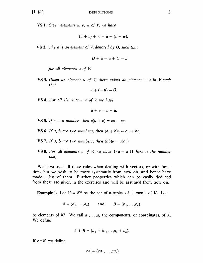
VS 1. Given elements u, v, w of V, we have
(u + v) + w = u + (v + w).
VS 2. There is an element of V, denoted by 0, such that
for all elements u of V.
VS 3. Given an element u of V, there exists an element - u in V such that
u+(-u)=O.
VS 4. For all elements u, v of V, we have
u + v = v + u.
VS 5. If c is a number, then c(u + v) = cu + cv.
VS 6. If a, b are two numbers, then (a + b)v = av + bv.
VS 7. If a, b are two numbers, then (ab)v = a(bv).
VS 8. For all elements u of V, we have 1· u = u (1 here is the number one).
We have used all these rules when dealing with vectors, or with functions but we wish to be more systematic from now on, and hence have made a list of them. Further properties which can be easily deduced from these are given in the exercises and will be assumed from now on.
Example 1. Let V = K n be the set of n-tuples of elements of K. Let
and
be elements of Kn. We call a 1, ••• ,an the components, or coordinates, of A. We define
If C E K we define
4 VECTOR SPACES [I, §l]
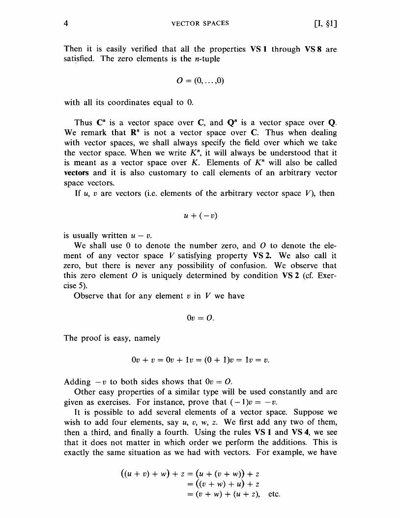
Then it is easily verified that all the properties VS 1 through VS 8 are sa t~sfied. The zero elements is the n-tu pIe
o = (0, ... ,0)
with all its coordinates equal to O.
Thus Cn is a vector space over C, and Qn is a vector space over Q. We remark that Rn is not a vector space over C. Thus when dealing with vector spaces, we shall always specify the field over which we take the vector space. When we write K n
, it will always be understood that it is meant as a vector space over K. Elements of K n will also be called vectors and it is also customary to call elements of an arbitrary vector space vectors.
If u, v are vectors (i.e. elements of the arbitrary vector space V), then
U + (-v)
is usually written u - v. We shall use 0 to denote the number zero, and 0 to denote the ele
ment of any vector space V satisfying property VS 2. We also call it zero, but there is never any possibility of confusion. We observe that this zero element 0 is uniquely determined by condition VS 2 (cf. Exercise 5).
Observe that for any element v in V we have
Ov = O.
The proof is easy, namely
Ov + v = Ov + Iv = (0 + l)v = Iv = v.
Adding - v to both sides shows that Ov = O. Other easy properties of a similar type will be used constantly and are
given as exercises. For instance, prove that (- l)v = - v. It is possible to add several elements of a vector space. Suppose we
wish to add four elements, say u, v, w, z. We first add any two of them, then a third, and finally a fourth. Using the rules VS 1 and VS 4, we see that it does not matter in which order we perform the additions. This is exactly the same situation as we had with vectors. For example, we have
«(u + v) + w) + z = (u + (v + w)) + z = «(v + w) + u) + z = (v + w) + (u + z), etc.
[I, §1] DEFINITIONS 5
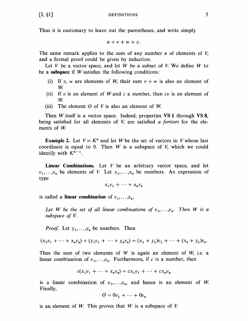
Thus it is customary to leave out the parentheses, and write simply
u + v + w + z.
The same remark applies to the sum of any number n of elements of V, and a formal proof could be given by induction.
Let V be a vector space, and let W be a subset of V. We define W to be a subspace if W satisfies the following conditions:
(i) If v, ware elements of W, their sum v + w is also an element of W.
(ii) If v is an element of Wand c a number, then cv is an element of W.
(iii) The element 0 of V is also an element of W
Then W itself is a vector space. Indeed, properties VS 1 through VS 8, being satisfied for all elements of V, are satisfied a fortiori for the elements of W
Example 2. Let V = Kn and let W be the set of vectors in V whose last coordinate is equal to O. Then W is a subspace of V, which we could identify with K n
-l
.
Linear Combinations. Let V be an arbitrary vector space, and let V l , .•. 'Vn be elements of V Let Xl' ... ,xn be numbers. An expression of type
is called a linear combination of v l , . .. ,vn •
Let W be the set of all linear combinations of V l , .•• ,Vn • Then W is a subspace of V.
Proof Let Yl' ... ,Yn be numbers. Then
Thus the sum of two elements of W is again an element of W, i.e. a linear combination of V l , ... ,Vn • Furthermore, if c is a number, then
is a linear combination of VI' ••• ,Vn , and hence is an element of W Finally,
o = OV l + ... + OVn
is an element of W. This proves that W is a subspace of V.
6 VECTOR SPACES [I, §1]
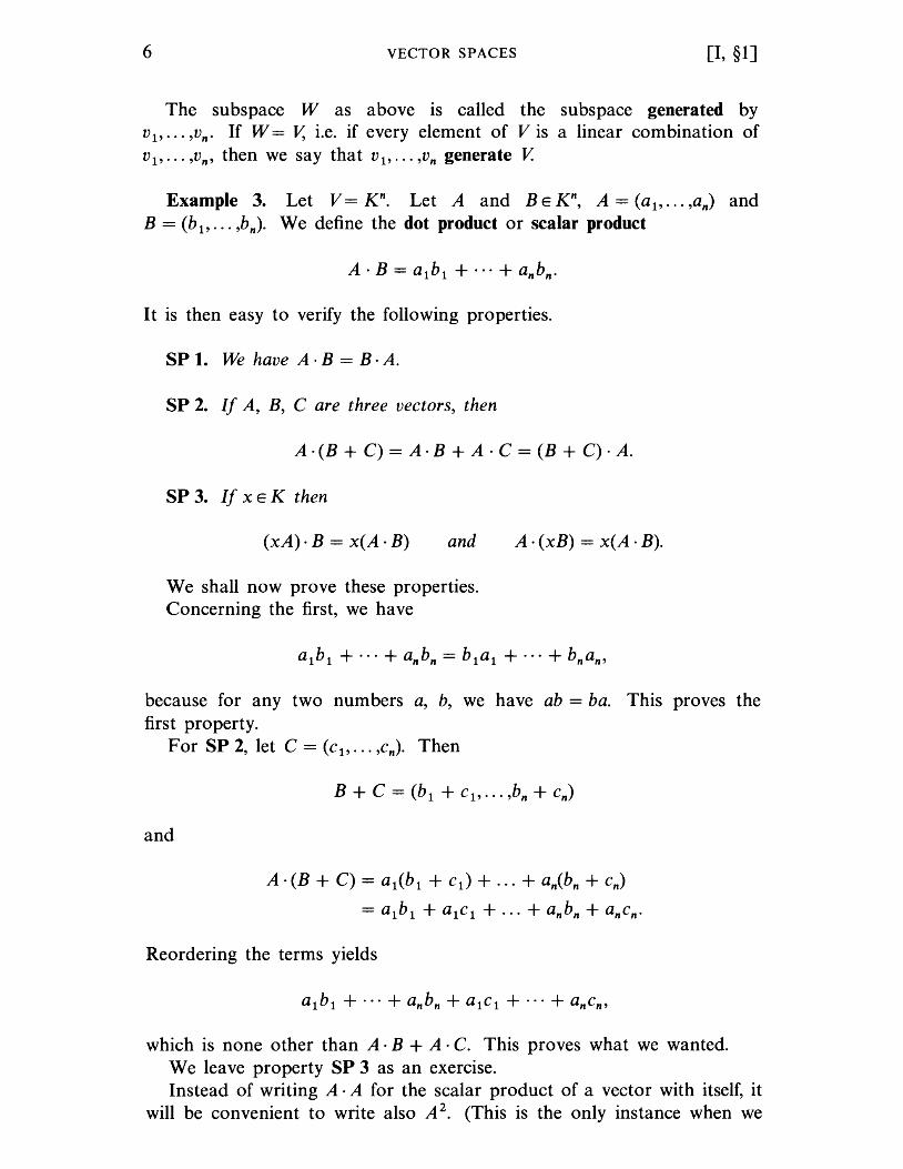
The subspace W as above is called the subspace generated by V l , ••• ,Vn • If W = V, i.e. if every element of V is a linear combination of V l , ••• ,Vn , then we say that V l , ... 'Vn generate V.
Example 3. Let V = Kn. Let A and BE K n, A = (a l , ... ,an) and B = (b l' ... ,b n). We define the dot product or scalar product
I t is then easy to verify the following properties.
SP 1. We have A· B = B· A.
SP 2. If A, B, C are three vectors, then
A . (B + C) = A· B + A . C = (B + C) . A.
SP 3. If x E K then
(xA)·B = x(A·B) and
We shall now prove these properties. Concerning the first, we have
A·(xB) = x(A·B).
because for any two numbers a, b, we have ab = ba. This proves the first property.
For SP 2, let C = (c l , ... ,cn). Then
and
A·(B + C) = al(b l + cl ) + ... + an(bn + cn)
= alb l + alc l + ... + anbn + ancn·
Reordering the terms yields
which is none other than A· B + A . C. This proves what we wanted. We leave property SP 3 as an exercise. Instead of writing A· A for the scalar product of a vector with itself, it
will be convenient to write also A 2• (This is the only instance when we
[I, §1] DEFINITIONS 7
allow ourselves such a notation. Thus A 3 has no meaning.) As an exercise, verify the following identities:
(A + B)2 = A2 + 2A· B + B2,
(A - B)2 = A2 - 2A· B + B2.
A dot product A· B may very well be equal to ° without either A or B being the zero vector. For instance, let A = (1, 2, 3) and B = (2, 1, -1). Then A·B = 0.
We define two vectors A, B to be perpendicular (or as we shall also say, orthogonal) if A· B = 0. Let A be a vector in K". Let W be the set of all elements B in K" such that B· A = 0, i.e. such that B is perpendicular to A. Then W is a subspace of K". To see this, note that o . A = 0, so that 0 is in W. Next, suppose that B, C are perpendicular to A. Then
(B + C)· A = B· A + C· A = 0,
so that B + C is also perpendicular to A. Finally, if x is a number, then
(xB)·A = x(B·A) = 0,
so that xB is perpendicular to A. This proves that W is a subspace of K".
Example 4. Function Spaces. Let S be a set and K a field. By a function of S into K we shall mean an association which to each element of S associates a unique element of K. Thus if f is a function of S into K, we express this by the symbols
f:S~K.
We also say that f is a K-valued function. Let V be the set of all functions of S into K. If f, g are two such functions, then we can form their sum f + g. It is the function whose value at an element x of S is f(x) + g(x). We write
(f + g)(x) = f(x) + g(x).
If c E K, then we define cf to be the function such that
(cf)(x) = cf(x).
Thus the value of cf at x is cf(x). It is then a very easy matter to verify that V is a vector space over K. We shall leave this to the reader. We
8 VECTOR SPACES [I, §1]
observe merely that the zero element of V is the zero function, i.e. the function f such that f(x) = 0 for all XES. We shall denote this zero function by o.
Let V be the set of all functions of R into R. Then V is a vector space over R. Let W be the subset of continuous functions. If f, g are continuous functions, then f + g is continuous. If c is a real number, then cf is continuous. The zero function is continuous. Hence W is a subspace of the vector space of all functions of R into R, i.e. W is a subspace of V.
Let U be the set of differentiable functions of R into R. If j, g are differentiable functions, then their sum f + g is also differentiable. If c is a real number, then cf is differentiable. The zero function is differentiable. Hence U is a subspace of V. In fact, U is a subspace of W, because every differentiable function is continuous.
Let V again be the vector space (over R) of functions from R into R. Consider the two functions et
" e2t. (Strictly speaking, we should say the
two functions f, g such that f(t) = et and get) = e2t for all t E R.) These functions generate a subspace of the space of all differentiable functions. The function 3et + 2e2t is an element of this subspace. So is the function 2et + ne2t
•
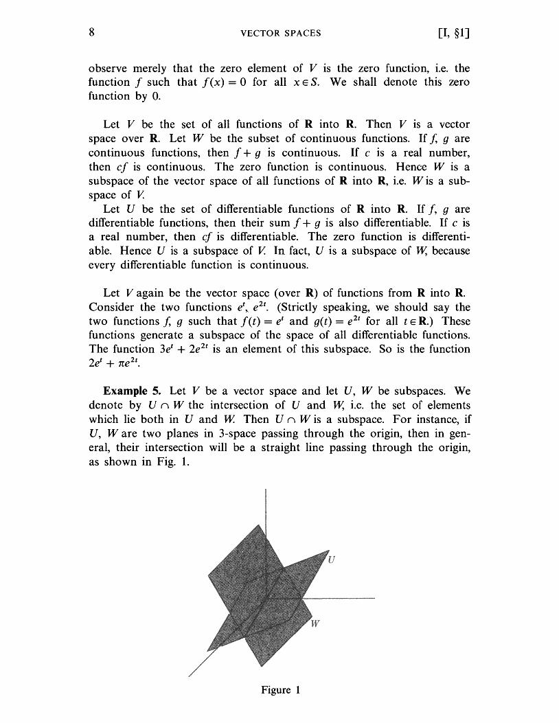
Example 5. Let V be a vector space and let U, W be subspaces. We denote by U n W the intersection of U and W, i.e. the set of elements which lie both in U and W. Then U n W is a subspace. For instance, if U, Ware two planes in 3-space passing through the origin, then in general, their intersection will be a straight line passing through the origin, as shown in Fig. 1.
Figure 1
[I, §1] DEFINITIONS 9
Example 6. Let U, W be subspaces of a vector space V. By
U+W
we denote the set of all elements u + w with U E U and w E W Then we leave it to the reader to verify that U + W is a subspace of V, said to be generated by U and W, and called the sum of U and W
I, §1. EXERCISES
1. Let V be a vector space. Using the properties VS 1 through VS 8, show that if c is a number, then cO = O.
2. Let c be a number i= 0, and v an element of V. Prove that if cv = 0, then v = o.
3. In the vector space of functions, what is the function satisfying the condition VS2?
4. Let V be a vector space and v, W two elements of V. If v + W = 0, show that W= -v.
5. Let V be a vector space, and v, w two elements of V such that v + w = v. Show that w = O.
6. Let A 1, A2 be vectors in Rn. Show that the set of all vectors B in Rn such that B is perpendicular to both A 1 and A2 is a subspace.
7. Generalize Exercise 6, and prove: Let A 1, ••• ,A, be vectors in Rn. Let W be the set of vectors B in Rn such that B· Ai = 0 for every i = 1, ... ,r. Show that W is a subspace of Rn.
8. Show that the following sets of elements in R 2 form subspaces. (a) The set of all (x, y) such that x = y. (b) The set of all (x, y) such that x - y = o. (c) The set of all (x, y) such that x + 4y = o.
9. Show that the following sets of elements in R 3 form subspaces. (a) The set of all (x, y, z) such that x + y + z = o. (b) The set of all (x, y, z) such that x = y and 2y = z. (c) The set of all (x, y, z) such that x + y = 3z.
10. If U, Ware subspaces of a vector space V, show that U n Wand U + Ware subspaces.
11. Let K be a subfield of a field L. Show that L is a vector space over K. In particular, C and R are vector spaces over Q.
12. Let K be the set of all numbers which can be written in the form a + b.j2, where a, b are rational numbers. Show that K is a field.
13. Let K be the set of all numbers which can be written in the form a + bi, where a, b are rational numbers. Show that K is a field.
10 VECTOR SPACES [I, §2]
14. Let c be a rational number> 0, and let y be a real number such that y2 = c. Show that the set of all numbers which can be written in the form a + by, where a, b are rational numbers, is a field.
I, §2. BASES
Let V be a vector space over the field K, and let v l' ... ,Vn be elements of V. We shall say that v l' ... 'Vn are linearly dependent over K if there exist elements a1, ••• ,an in K not all equal to ° such that
If there do not exist such numbers, then we say that V1, ••• ,Vn are linearly independent. In other words, vectors V 1, •.• ,Vn are linearly independent if and only if the following condition is satisfied:
Whenever a1, ••• ,an are numbers such that
then ai = ° fot all i = 1, ... ,no
Example 1. Let V = K n and consider the vectors
E 1 = (1, 0, ... ,0)
En = (0, 0, ... ,1).
Then E 1' ... ,En are linearly independent. Indeed, let a1, ••• ,an be numbers such that
Since
it follows that all ai = 0.
Example 2. Let V be the vector space of all functions of a variable t. Let f1' ... ,fn be n functions. To say that they are linearly dependent is to say that there exists n numbers a1, ••• ,an not all equal to ° such that
for all values of t.
[I, §2] BASES 11
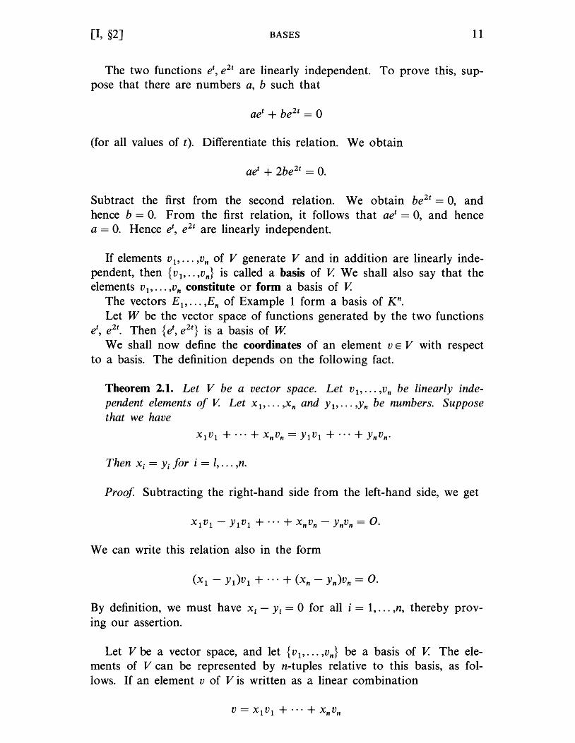
The two functions et, e2t are linearly independent. To prove this, sup
pose that there are numbers a, b such that
(for all values of t). Differentiate this relation. We obtain
Subtract the first from the second relation. We obtain be2t = 0, and hence b = O. From the first relation, it follows that aet = 0, and hence a = O. Hence et
, e2t are linearly independent.
If elements v1, ••• 'Vn of V generate V and in addition are linearly independent, then {v 1, •• ,vn} is called a basis of V. We shall also say that the elements v1, ••• 'Vn constitute or form a basis of V.
The vectors E 1, ••• ,En of Example 1 form a basis of Kn. Let W be the vector space of functions generated by the two functions
et, e2t
• Then {et, e2t
} is a basis of W We shall now define the coordinates of an element v E V with respect
to a basis. The definition depends on the following fact.
Theorem 2.1. Let V be a vector space. Let V 1, ••• 'Vn be linearly independent elements of V. Let Xl' ... ,xn and Y1' ... ,Yn be numbers. Suppose that we have
Then Xi = Yi for i = 1, ... ,no
Proof Subtracting the right-hand side from the left-hand side, we get
We can write this relation also in the form
By definition, we must have Xi - Yi = 0 for all i = 1, ... ,n, thereby proving our assertion.
Let V be a vector space, and let {v 1, ••• ,vn } be a basis of V. The elements of V can be represented by n-tuples relative to this basis, as follows. If an element v of V is written as a linear combination
12 VECTOR SPACES [I, §2]
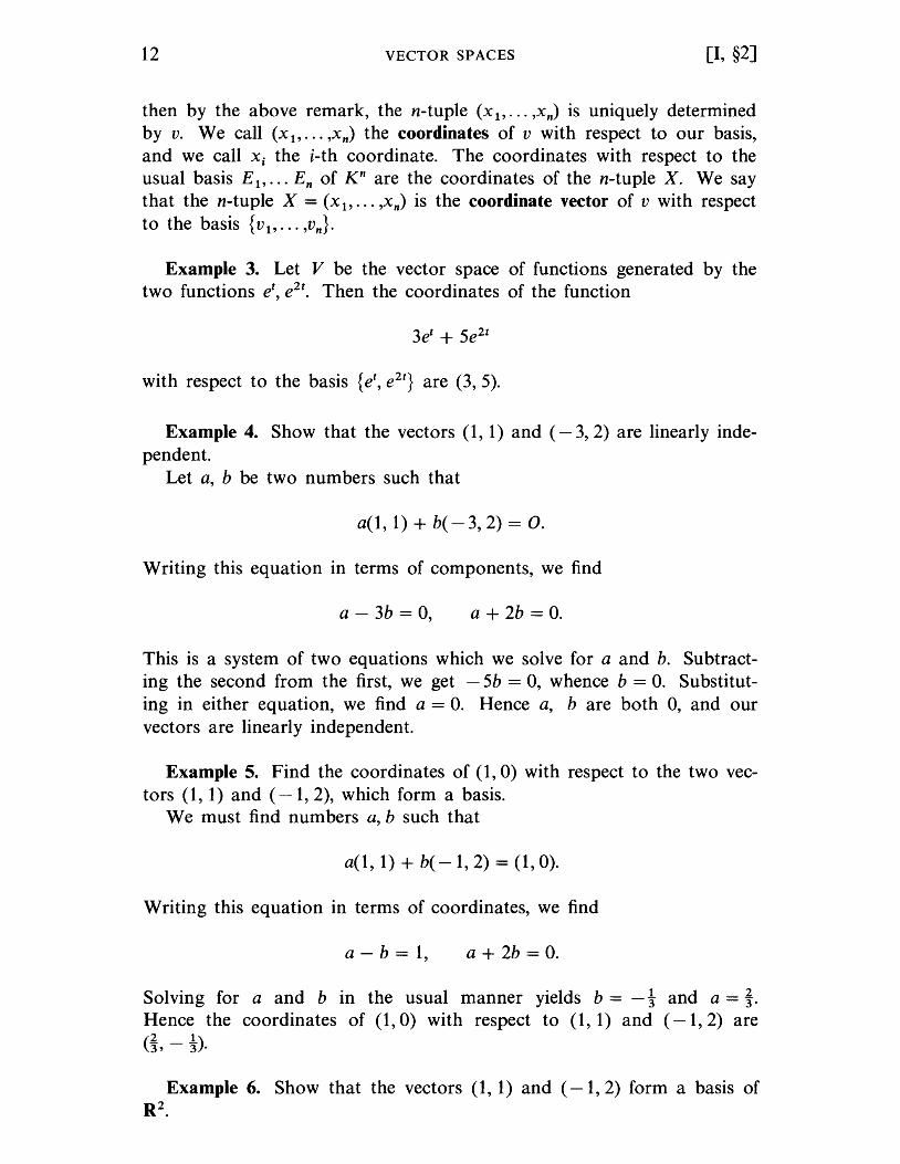
then by the above remark, the n-tuple (Xl"" ,Xn) is uniquely determined by v. We call (x 1, ... ,xn) the coordinates of v with respect to our basis, and we call Xi the i-th coordinate. The coordinates with respect to the usual basis E 1, ••• En of K n are the coordinates of the n-tuple X. We say that the n-tuple X = (Xl' ... ,Xn) is the coordinate vector of v with respect to the basis {v 1, ••• ,Vn }.
Example 3. Let V be the vector space of functions generated by the two functions et
, e2t• Then the coordinates of the function
with respect to the basis {et, e2t
} are (3, 5).
Example 4. Show that the vectors (1, 1) and (- 3, 2) are linearly independent.
Let a, b be two numbers such that
a( 1, 1) + b( - 3, 2) = o.
Writing this equation in terms of components, we find
a - 3b = 0, a + 2b = O.
This is a system of two equations which we solve for a and b. Subtracting the second from the first, we get - 5b = 0, whence b = O. Substituting in either equation, we find a = O. Hence a, b are both 0, and our vectors are linearly independent.
Example 5. Find the coordinates of (1, 0) with respect to the two vectors (1, 1) and (-1, 2), which form a basis.
We must find numbers a, b such that
a(l, 1) + b( -1, 2) = (1,0).
Writing this equation in terms of coordinates, we find
a - b = 1, a + 2b = O.
Solving for a and b in the usual manner yields b = -t and a = ~. Hence the coordinates of (1,0) with respect to (1, 1) and (-1, 2) are (~, - t)·
Example 6. Show that the vectors (1, 1) and (-1, 2) form a basis of R2.
[I, §2] BASES 13
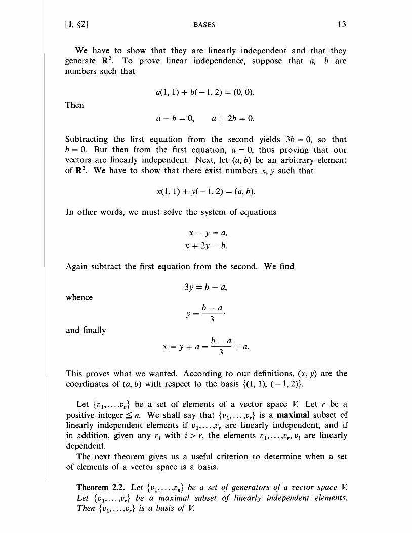
We have to show that they are linearly independent and that they generate R2. To prove linear independence, suppose that a, bare numbers such that
a(1, 1) + b( -1, 2) = (0, 0).
Then
a - b = 0, a + 2b = O.
Subtracting the first equation from the second yields 3b = 0, so that b = O. But then from the first equation, a = 0, thus proving that our vectors are linearly independent. Next, let (a, b) be an arbitrary element of R2. We have to show that there exist numbers x, y such that
x(1, 1) + y( -1, 2) = (a, b).
In other words, we must solve the system of equations
x-y=a,
x + 2y = b.
Again subtract the first equation from the second. We find
whence
and finally
3y = b - a,
b-a y=--'
3
b-a x=y+a=-3-+ a.
This proves what we wanted. According to our definitions, (x, y) are the coordinates of (a, b) with respect to the basis {(1, 1), (-1, 2)}.
Let {v l , ... ,vn } be a set of elements of a vector space V. Let r be a positive integer < n. We shall say that {v l , ... ,v,} is a maximal subset of linearly independent elements if V l , ... ,v, are linearly independent, and if in addition, given any Vi with i > r, the elements V l , .•• ,v" Vi are linearly dependent.
The next theorem gives us a useful criterion to determine when a set of elements of a vector space is a basis.
Theorem 2.2. Let {v l , ... ,vn } be a set of generators of a vector space V. Let {v l , ... ,v,} be a maximal subset of linearly independent elements. Then {v l , ... ,v,} is a basis of V.
14 VECTOR SPACES [I, §2]
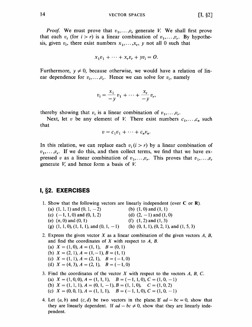
Proof We must prove that V 1 , ••• 'Vr generate V. We shall first prove that each Vi (for i > r) is a linear combination of V 1, ••• ,Vr • By hypothesis, given Vi' there exist numbers Xl' ... ,Xr , Y not all 0 such that
Furthermore, y i= 0, because otherwise, we would have a relation of linear dependence for Vi' ••• ,vr • Hence we can solve for Vi' namely
Xl Xr Vi = - V 1 + ... + - Vr ,
-y -y
thereby showing that Vi is a linear combination of V 1, ••• ,Vr •
Next, let V be any element of V. There exist numbers C 1 , ••• 'Cn such that
In this relation, we can replace each Vi (i > r) by a linear combination of V 1, ••• ,Vr • If we do this, and then collect terms, we find that we have expressed V as a linear combination of V 1, ••• ,Vr • This proves that V 1, ... ,Vr
generate V, and hence form a basis of V.
I, §2. EXERCISES
1. Show that the following vectors are linearly independent (over C or R). (a) (1,1,1) and (0,1, -2) (b) (1,0) and (1,1) (c) (-1, 1,0) and (0, 1, 2) (d) (2, -1) and (1,0) (e) (n, 0) and (0,1) (f) (1,2) and (1, 3) (g) (1, 1, 0), (1, 1, 1), and (0, 1, -1) (h) (0, 1, 1), (0, 2, 1), and (1, 5, 3)
2. Express the given vector X as a linear combination of the given vectors A, B, and find the coordinates of X with respect to A, B. (a) X = (1,0), A = (1, 1), B = (0, 1) (b) X = (2,1), A = (1,-1), B = (1,1) (c) X = (1, 1), A = (2, 1), B = (-1,0) (d) X = (4,3), A = (2, 1), B = (-1,0)
3. Find the coordinates of the vector X with respect to the vectors A, B, C. (a) X = (1,0,0), A = (1, 1, 1), B = ( -1, 1,0), C = (1,0, -1) (b) X = (1, 1, 1), A = (0, 1, -1), B = (1, 1,0), C = (1,0,2) (c) X = (0,0, 1), A = (1, 1, 1), B = (-1, 1,0), C = (1,0, -1)
4. Let (a, b) and (c, d) be two vectors in the plane. If ad - bc = 0, show that they are linearly dependent. If ad - bc # 0, show that they are linearly independent.
[I, §3] DIMENSION OF A VECTOR SPACE 15
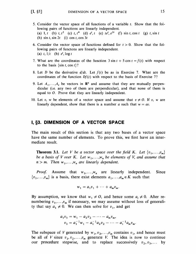
5. Consider the vector space of all functions of a variable t. Show that the following pairs of functions are linearly independent. (a) 1, t (b) t, t 2 (c) t, t4 (d) et, t (e) tet, e2t (f) sin t, cos t (g) t, sin t (h) sin t, sin 2t (i) cos t, cos 3t
6. Consider the vector space of functions defined for t > O. Show that the following pairs of functons are linearly independent. (a) t, lit (b) e" log t
7. What are the coordinates of the function 3 sin t + 5 cos t = f(t) with respect to the basis {sin t, cos t}?
8. Let D be the derivative dldt. Let f(t) be as in Exercise 7. What are the coordinates of the function Df(t) with respect to the basis of Exercise 7?
9. Let A 1"" ,A, be vectors in Rn and assume that they are mutually perpendicular (i.e. any two of them are perpendicular), and that none of them is equal to O. Prove that they are linearly independent.
10. Let v, w be elements of a vector space and assume that v # O. If v, ware linearly dependent, show that there is a number a such that w = avo
I, §3. DIMENSION OF A VECTOR SPACE
The main result of this section is that any two bases of a vector space have the same number of elements. To prove this, we first have an intermedia te res ul t.
Theorem 3.1. Let V be a vector space over the field K. Let {v 1, ... ,vm} be a basis of V over K. Let w1, ••• ,Wn be elements of V, and assume that n > m. Then W 1, .•. ,Wn are linearly dependent.
Proof Assume that W 1, ... ,Wn are linearly independent. Since {v 1, . .. ,vm} is a basis, there exist elements a1, ... ,am E K such that
By assumption, we know that W 1 i= 0, and hence some ai i= O. After renumbering V 1, ••• ,Vm if necessary, we may assume without loss of generality that say a1 i= O. We can then solve for V 1, and get
a1v1 = W 1 - a2 v2 - ••• - amvm, -1 -1 -1 v1=a1 w1-a1 a2 v2 -···-a1 amvm·
The subspace of V generated by W 1, V 2, ... ,Vm contains V 1, and hence must be all of V since V 1, V 2 , ... ,Vm generate V. The idea is now to continue our procedure stepwise, and to replace successively V 2 , V3 ,... by
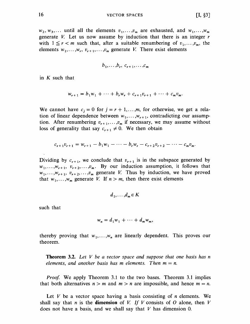
16 VECTOR SPACES [I, §3]
W 2 , W 3 , ••• until all the elements V 1, ••• 'Vm are exhausted, and W 1, ••• ,Wm
generate V. Let us now assume by induction that there is an integer r with 1 < r < m such that, after a suitable renumbering of V1, ••• ,Vm , the elements W 1, ... ,Wr , V r + 1' ... ,Vm generate V. There exist elements
in K such that
We cannot have cj = 0 for j = r + 1, ... ,m, for otherwise, we get a rela-tion of linear dependence between W 1, ... ,Wr + l' contradicting our assump-tion. After renumbering vr + 1' ... ,vm if necessary, we may assume without loss of generality that say cr + 1 i= O. We then obtain
Dividing by Cr + l' we conclude that vr + 1 is in the subspace generated by w 1, ••. ,Wr + l' V r + 2,··· ,Vm • By our induction assumption, it follows that W 1, ••• 'W r + 1, V r + 2 , ••• ,Vm generate V. Thus by induction, we have proved that W l , ... ,Wm generate V. If n > m, then there exist elements
such that
thereby proving that W 1, ... ,Wn are linearly dependent. This proves our theorem.
Theorem 3.2. Let V be a vector space and suppose that one basis has n elements, and another basis has m elements. Then m = n.
Proof We apply Theorem 3.1 to the two bases. Theorem 3.1 implies that both alternatives n > m and m > n are impossible, and hence m = n.
Let V be a vector space having a basis consisting of n elements. We shall say that n is the dimension of V. If V consists of 0 alone, then V does not have a basis, and we shall say that V has dimension O.
[I, §3] DIMENSION OF A VECTOR SPACE 17
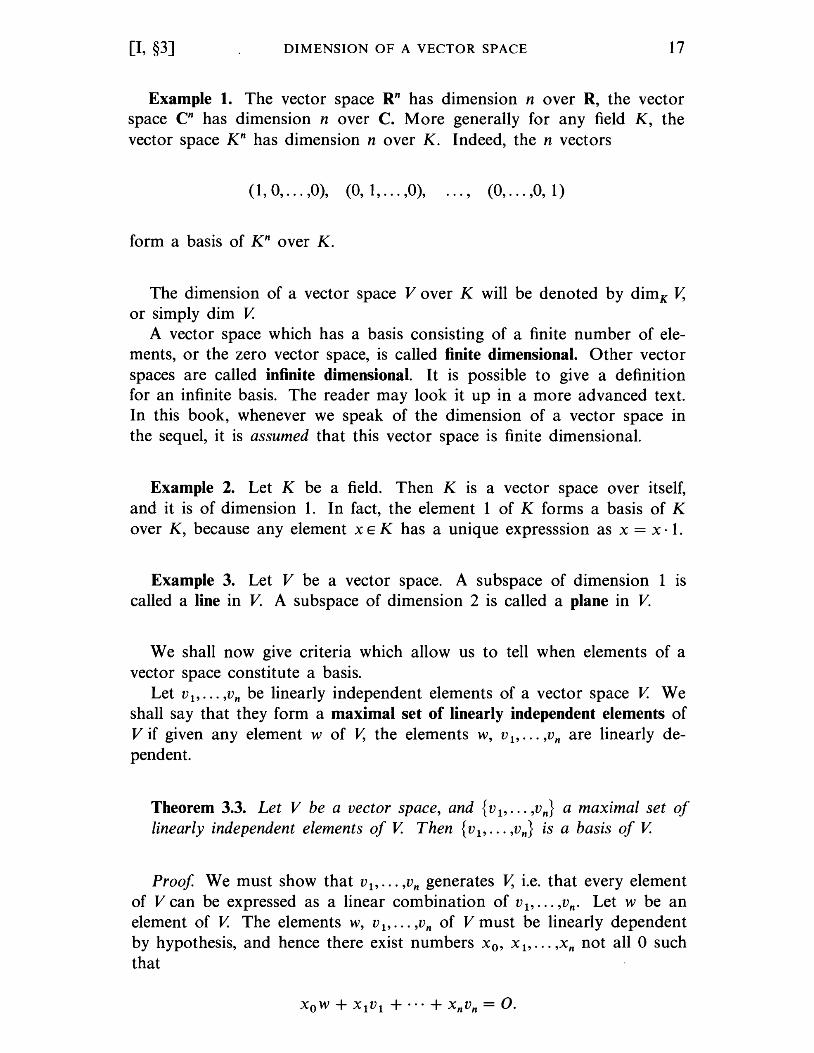
Example 1. The vector space Rn has dimension n over R, the vector space Cn has dimension n over C. More generally for any field K, the vector space K n has dimension n over K. Indeed, the n vectors
(1, 0, ... ,0), (0, 1, ... ,0), ... , (0, ... ,0, 1)
form a basis of Kn over K.
The dimension of a vector space V over K will be denoted by dimK V, or simply dim V.
A vector space which has a basis consisting of a finite number of elements, or the zero vector space, is called finite dimensional. Other vector spaces are called infinite dimensional. It is possible to give a definition for an infinite basis. The reader may look it up in a more advanced text. In this book, whenever we speak of the dimension of a vector space in the sequel, it is assumed that this vector space is finite dimensional.
Example 2. Let K be a field. Then K is a vector space over itself, and it is of dimension 1. In fact, the element 1 of K forms a basis of K over K, because any element x E K has a unique expresssion as x = X· 1.
Example 3. Let V be a vector space. A subspace of dimension 1 is called a line in V. A subspace of dimension 2 is called a plane in V.
We shall now give criteria which allow us to tell when elements of a vector space constitute a basis.
Let V 1, ••• ,Vn be linearly independent elements of a vector space V. We shall say that they form a maximal set of linearly independent elements of V if given any element w of V, the elements w, v 1, ... ,Vn are linearly dependent.
Theorem 3.3. Let V be a vector space, and {v 1, ••• ,vn} a maximal set of linearly independent elements of V. Then {v 1, ••• ,vn} is a basis of V.
Proof. We must show that V 1, ••• ,vn generates V, i.e. that every element of V can be expressed as a linear combination of V 1, ••• ,Vn • Let w be an element of V. The elements w, V 1, ••• 'Vn of V must be linearly dependent by hypothesis, and hence there exist numbers X o, x 1, ... ,Xn not all Osuch that
18 VECTOR SPACES [I, §3]
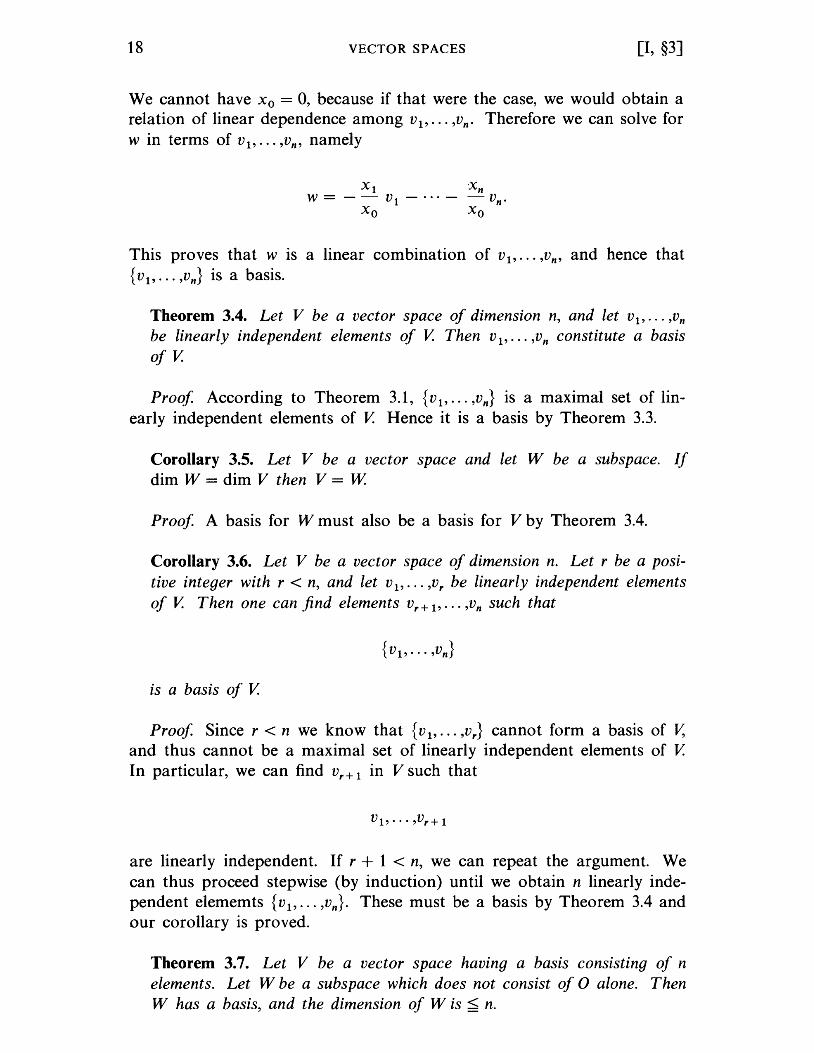
We cannot have Xo = 0, because if that were the case, we would obtain a relation of linear dependence among v1 , ••• ,vn • Therefore we can solve for w in terms of v1, ••• ,Vn , namely
Xl Xn W = - - V 1 - ••• - - Vn •
Xo Xo
This proves that w is a linear combination of V 1, ... ,Vn , and hence that {v 1 , ••• ,vn } is a basis.
Theorem 3.4. Let V be a vector space of dimension n, and let V 1,··· ,Vn
be linearly independent elements of V. Then V 1, ... ,vn constitute a basis of V.
Proof According to Theorem 3.1, {v 1, ••• ,vn } is a maximal set of linearly independent elements of V. Hence it is a basis by Theorem 3.3.
Corollary 3.5. Let V be a vector space and let W be a subspace. If dim W = dim V then V = W
Proof A basis for W must also be a basis for V by Theorem 3.4.
Corollary 3.6. Let V be a vector space of dimension n. Let r be a positive integer with r < n, and let v1, •.• ,Vr be linearly independent elements of V. Then one can find elements vr + 1' ... ,vn such that
is a basis of V.
Proof Since r < n we know that {v 1, ••• ,vr } cannot form a basis of V, and thus cannot be a maximal set of linearly independent elements of V. In particular, we can find Vr + 1 in V such that
are linearly independent. If r + 1 < n, we can repeat the argument. We can thus proceed stepwise (by induction) until we obtain n linearly independent elememts {v 1 , ••• ,vn }. These must be a basis by Theorem 3.4 and our corollary is proved.
Theorem 3.7. Let V be a vector space having a basis consisting of n elements. Let W be a subspace which does not consist of 0 alone. Then W has a basis, and the dimension of W is < n.
[I, §4] SUMS AND DIRECT SUMS 19
Proof Let W 1 be a non-zero element of W If {w l} is not a maximal set of linearly independent elements of W, we can find an element W 2 of W such that Wl' W2 are linearly independent. Proceeding in this manner, one element at a time, there must be an integer m < n such that we can find linearly independent elements Wl' W 2 , ••• ,Wm , and such that
is a maxmal set of linearly independent elements of W (by Theorem 3.1 we cannot go on indefinitely finding linearly independent elements, and the number of such elements is at most n). If we now use Theorem 3.3, we conclude that {w l , ... ,wm } is a basis for W
I, §4. SUMS AND DIRECT SUMS
Let V be a vector space over the field K. Let U, W be subspaces of V. We define the sum of U and W to be the subset of V consisting of all sums u + W with UE U and WE W We denote this sum by U + W It is a subspace of V. Indeed, if U l , U 2 E U and Wl' W2 E W then
If cEK, then
Finally, 0 + 0 E W This proves that U + W is a subspace. We shall say that V is a direct sum of U and W if for every element v
of V there exist unique elements U E U and WE W such that v = U + w.
Theorem 4.1. Let V be a vector space over the field K, and let U, W be subspaces. If U + W = V, and if U n W = {O}, then V is the direct sum of U and W
Proof Given v E V, by the first assumption, there exist elements u E U and W E W such that v = U + w. Thus V is the sum of U and W. To prove it is the direct sum, we must show that these elements u, ware uniquely determined. Suppose there exist elements u' E U and w' E W such that v = u' + w'. Thus
u + W = u' + w'.
Then
u - u' = w' - w.
20 VECTOR SPACES [I, §4]
But u - U' E U and w' - W E W. By the second assumption, we conclude that u - u' = 0 and w' - w = 0, whence u = u' and w = w', thereby proving our theorem.
As a matter of notation, when V is the direct sum of subspaces U, W we write
V=U(f)w.
Theorem 4.2. Let V be a finite dimensional vector space over the field K. Let W be a subspace. Then there exists a subspace U such that V is the direct sum of Wand U.
Proof We select a basis of W, and extend it to a basis of V, uSIng Corollary 3.6. The assertion of our theorem is then clear. In the notation of that theorem, if {v 1, ••• ,vr } is a basis of W, then we let U be the space generated by {vr + 1"" ,Vn}.
We note that given the subspace W, there exist usually many subspaces U such that V is the direct sum of Wand U. (For examples, see the exercises.) In the section when we discuss orthogonality later in this book, we shall use orthogonality to determine such a subspace.
Theorem 4.3. If V is a finite dimensional vector space over K, and is the direct sum of subspaces U, W then
dim V= dim U + dim W.
Proof Let {u 1, ••• ,ur } be a basis of U, and {w 1, ••• ,ws} a basis of W. Every element of U has a unique expression as a linear combination X 1U 1 + ... + XrUr ' with Xi E K, and every element of W has a unique expression as a linear combination Y1 W 1 + ... + Ys Ws with Yj E K. Hence by definition, every element of V has a unique expression as a linear combination
thereby proving that u1, ••• ,ur , w 1, ••• ,Ws is a basis of V, and also proving our theorem.
Suppose now that U, Ware arbitrary vector spaces over the field K (i.e. not necessarily subspaces of some vector space). We let U x W be the set of all pairs (u, w) whose first component is an element u of U and whose second component is an element w of W. We define the addition of such pairs componentwise, namely, if (u 1, w1 ) E U x Wand (u2 , w 2 ) E U x W we define
[I, §4] SUMS AND DIRECT SUMS 21
If C E K we define the product C(U I , WI) by
It is then immediately verified that U x W is a vector space, called the direct product of U and W When we discuss linear maps, we shall compare the direct product with the direct sum.
If n is a positive integer, written as a sum of two positive integers, n = r + s, then we see that K n is the direct product Kr x K S
•
We note that
dim (U x W) = dim U + dim W
The proof is easy, and is left to the reader. Of course, we can extend the notion of direct sum and direct product
of several factors. Let VI' ... ' v" be subspaces of a vector space V. We say that V is the direct sum
n
V= ffi~= VI E9···E9Y" i= 1
if every element v E V has a unique expression as a sum
with Vi E ~.
A "unique expression" means that if
V = V/l + ... + v~
then v~ = Vi for i = 1, ... ,no Similarly, let WI' ... ' ~ be vector spaces. We define their direct pro-
duct n
n~=WIX ... X~ i= I
to be the set of n-tuples (w l , ... ,wn) with Wi E~. Addition is defined componentwise, and multiplication by scalars is also defined componen twise. Then this direct product is a vector space.
22 VECTOR SPACES [I, §4]
I, §4. EXERCISES
1. Let V = R 2, and let W be the subspace generated by (2, 1). Let U be the subspace generated by (0, 1). Show that V is the direct sum of Wand U. If U' is the subspace generated by (1, 1), show that V is also the direct sum of Wand U'.
2. Let V = K3 for some field K. Let W be the subspace generated by (1, 0, 0), and let U be the subspace generated by (1, 1, 0) and (0, 1, 1). Show that V is the direct sum of Wand U.
3. Let A, B be two vectors in R2, and assume neither of them is O. If there is no number c such that cA = B, show that A, B form a basis of R2, and that R 2 is a direct sum of the subspaces generated by A and B respectively.
4. Prove the last assertion of the section concerning the dimension of U x W If {u 1, ••• ,ur } is a basis of U and {w 1, •.• ,ws} is a basis of W, what is a basis of U x W?
CHAPTER II
Matrices
II, §1. THE SPACE OF MATRICES
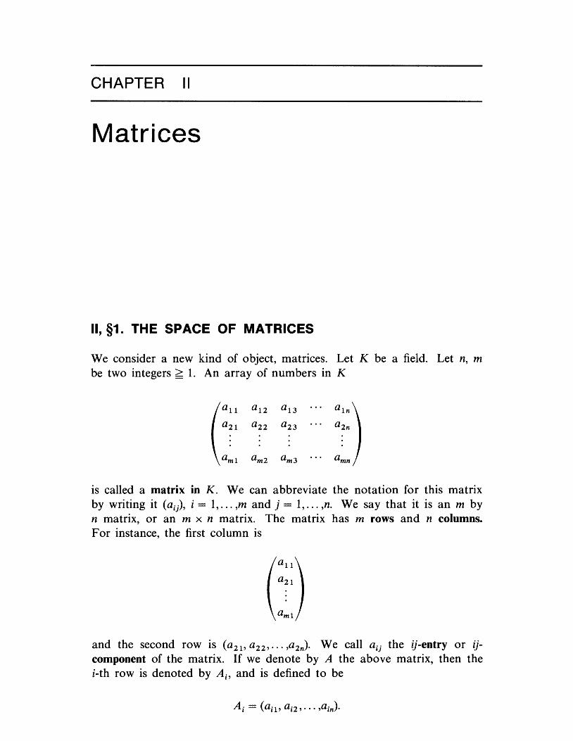
We consider a new kind of object, matrices. Let K be a field. Let n, m be two integers > 1. An array of numbers in K
all a 12 a 13 a ln
a21 a22 a23 a2n
is called a matrix in K. We can abbreviate the notation for this matrix by writing it (aij), i = 1, ... ,m and j = 1, ... ,no We say that it is an m by n matrix, or an m x n matrix. The matrix has m rows and n columns. For instance, the first column is
and the second row is (a 21 , a22 , ••. ,a2n). We call aij the ij-entry or ijcomponent of the matrix. If we denote by A the above matrix, then the i-th row is denoted by Ai' and is defined to be
24 MATRICES
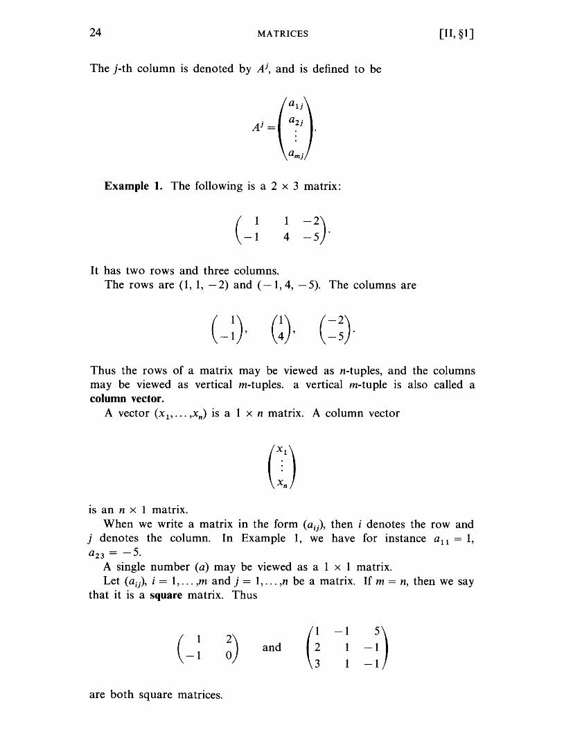
The j-th column is denoted by Ai, and is defined to be
Example 1. The following is a 2 x 3 matrix:
It has two rows and three columns.
1
4 -2) -5 .
The rows are (1, 1, - 2) and (-1, 4, - 5). The columns are
[II, §1]
Thus the rows of a matrix may be viewed as n-tuples, and the columns may be viewed as vertical m-tu pIes. a vertical m-tu pIe is also called a column vector.
A vector (Xl' ... ,Xn) is a 1 x n matrix. A column vector
is an n x 1 matrix. When we write a matrix in the form (a ii), then i denotes the row and
j denotes the column. In Example 1, we have for instance all = 1, a23 = -5.
A single number (a) may be viewed as a 1 x 1 matrix. Let (aij), i = 1, ... ,m and j = 1, ... ,n be a matrix. If m = n, then we say
that it is a square matrix. Thus
~) and
are both square matrices.
(~ -1
1
1 -~) -1
[II, §1] THE SPACE OF MATRICES 25
We have a zero matrix in which aij = 0 for all i, j. It looks like this:
000 0 o 0 0 0
o 0 0 0
We shall write it o. We note that we have met so far with the zero number, zero vector, and zero matrix.
We shall now define addition of matrices and multiplication of matrices by numbers.
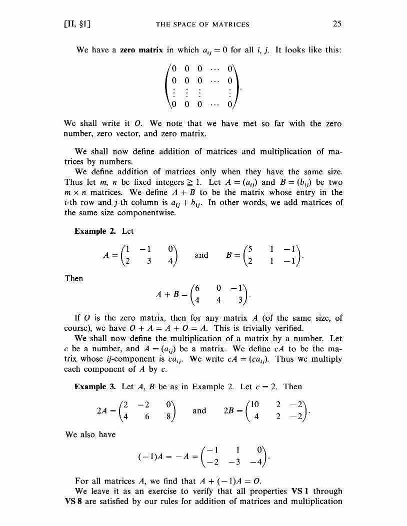
We define addition of matrices only when they have the same size. Thus let m, n be fixed integers > 1. Let A = (aij) and B = (bij) be two m x n matrices. We define A + B to be the matrix whose entry in the i-th row and j-th column is aij + bij. In other words, we add matrices of the same size componentwise.
Example 2. Let
A=G -1 ~) B=G
1 -1) 3
and 1 -1 .
Then
A + B = (: 0 -1) 4 3 .
If 0 is the zero matrix, then for any matrix A (of the same size, of course), we have 0 + A = A + 0 = A. This is trivially verified.
We shall now define the multiplication of a matrix by a number. Let c be a number, and A = (aij) be a matrix. We define cA to be the matrix whose ij-component is caij. We write cA = (caij). Thus we multiply each component of A by c.
Example 3. Let A, B be as in Example 2. Let c = 2. Then
2A = (~ -2 ~) CO 2 -2)
6 and 2B = 4 2 -2 .
We also have
(-1 1 -~) (-1)A = -A =
-3 -2
For all matrices A, we find that A + ( -1)A = o. We leave it as an exercise to verify that all properties VS 1 through
VS 8 are satisfied by our rules for addition of matrices and multiplication
26 MATRICES [II, §1]
of matrices by elements of K. The main thing to observe here is that addition of matrices is defined in terms of the components, and for the addition of components, the conditions analogous to VS 1 through VS 4 are satisfied. They are standard properties of numbers. Similarly, VS 5 through VS 8 are true for multiplication of matrices by elements of K, because the corresponding properties for the multiplication of elements of K are true.
We see that the matrices (of a given size m x n) with components in a field K form a vector space over K which we may denote by Matm x n(K).
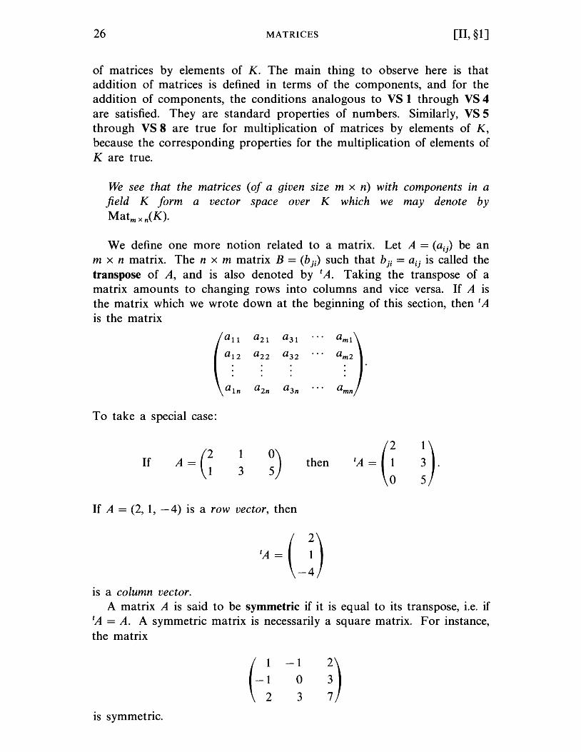
We define one more notion related to a matrix. Let A = (aij) be an m x n matrix. The n x m matrix B = (b ji ) such that bji = aij is called the transpose of A, and is also denoted by t A. Taking the transpose of a matrix amounts to changing rows into columns and vice versa. If A is the matrix which we wrote down at the beginning of this section, then l A is the matrix
To take a special case:
If
all a21 a31 ami a12 a22 a32 am2
1
3 ~) then
If A = (2, 1, -4) is a row vector, then
is a column vector. A matrix A is said to be symmetric if it is equal to its transpose, i.e. if
lA = A. A symmetric matrix is necessarily a square matrix. For instance, the matrix
(-~ is symmetric.
-1
o 3 ~)
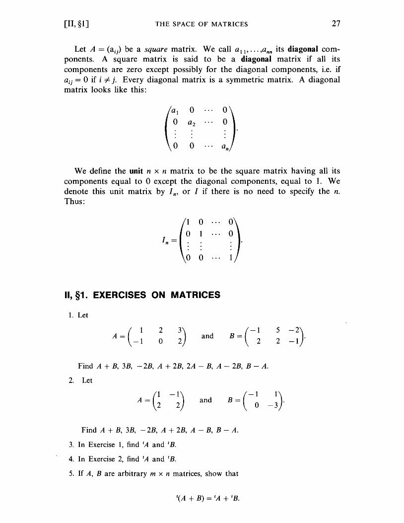
[II, §1] THE SPACE OF MATRICES 27
Let A = (aij) be a square matrix. We call all' ... ,ann its diagonal components. A square matrix is said to be a diagonal matrix if all its components are zero except possibly for the diagonal components, i.e. if aij = 0 if i =1= j. Every diagonal matrix is a symmetric matrix. A diagonal matrix looks like this:
We define the unit n x n matrix to be the square matrix having all its components equal to 0 except the diagonal components, equal to 1. We denote this unit matrix by In' or I if there is no need to specify the n. Thus:
I = n
100 o 1 0
001
II, §1. EXERCISES ON MATRICES
1. Let
A = ( 1 -1
2
o ~) and B= (-1
2
Find A + B, 3B, - 2B, A + 2B, 2A - B, A - 2B, B - A.
2. Let
5 -2) 2 -1·
and (-1 1) B = 0 -3·
Find A + B, 3B, - 2B, A + 2B, A - B, B - A.
3. In Exercise 1, find tA and t B.
4. In Exercise 2, find tA and t B.
5. If A, B are arbitrary m x n matrices, show that
28 MATRICES [II, § 1]
6. If c is a number, show that
7. If A = (aij ) is a square matrix, then the elements aii are called the diagonal elements. How do the diagonal elements of A and tA differ?
8. Find teA + B) and tA + tB in Exercise 2.
9. Find A + tA and B + tB in Exercise 2.
10. Show that for any square matrix A, the matrix A + tA is symmetric.
11. Write down the row vectors and column vectors of the matrices A, B in Exercise 1.
12. Write down the row vectors and column vectors of the matrices A, B In Exercise 2.
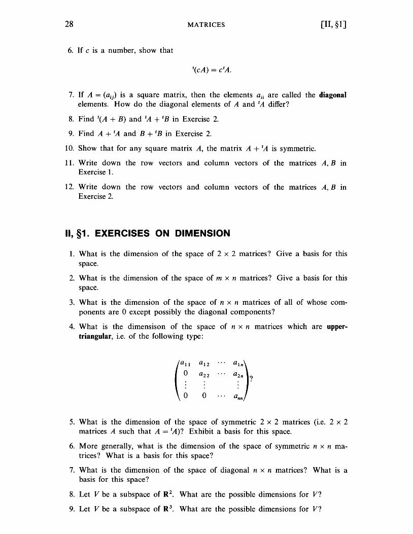
II, §1. EXERCISES ON DIMENSION
1. What is the dimension of the space of 2 x 2 matrices? Give a basis for this space.
2. What is the dimension of the space of m x n matrices? Give a basis for this space.
3. What is the dimension of the space of n x n matrices of all of whose components are 0 except possibly the diagonal components?
4. What is the dimensison of the space of n x n matrices which are uppertriangular, i.e. of the following type:
a 12 ...
a
l
") a22 ...
a~n ?
0 ann
5. What is the dimension of the space of symmetric 2 x 2 matrices (i.e. 2 x 2 matrices A such that A = tA)? Exhibit a basis for this space.
6. More generally, what is the dimension of the space of symmetric n x n matrices? What is a basis for this space?
7. What is the dimension of the space of diagonal n x n matrices? What is a basis for this space?
8. Let V be a subspace of R 2 • What are the possible dimensions for V?
9. Let V be a subspace of R 3 . What are the possible dimensions for V?
[II, §2] LINEAR EQUATIONS 29
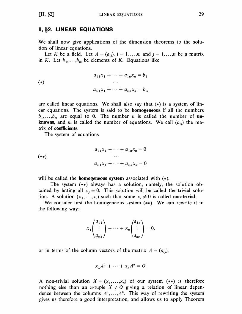
II, §2. LINEAR EQUATIONS
We shall now give applications of the dimension theorems to the solution of linear equations.
Let K be a field. Let A = (a ij), i = 1, ... ,m and j = 1, ... ,n be a matrix in K. Let bl , ... ,bm be elements of K. Equations like
are called linear equations. We shall also say that (*) is a system of linear equations. The system is said to be homogeneous if all the numbers bl , ... ,bm are equal to O. The number n is called the number of unknowns, and m is called the number of equations. We call (a ij) the matrix of coefficients.
The system of equations
a lX l + ... + a x = 0 m mn n
will be called the homogeneous system associated with (*). The system (**) always has a solution, namely, the solution ob
tained by letting all Xj = o. This solution will be called the trivial solution. A solution (Xl' ... ,xn) such that some Xi =1= 0 is called non-trivial.
We consider first the homogeneous system (**). We can rewrite it in the following way:
or in terms of the column vectors of the matrix A = (aij),
A non-trivial solution X = (Xl' ... ,xn ) of our system (**) is therefore nothing else than an n-tuple X =1= 0 giving a relation of linear dependence between the columns A l, ... ,An. This way of rewriting the system gives us therefore a good interpretation, and allows us to apply Theorem
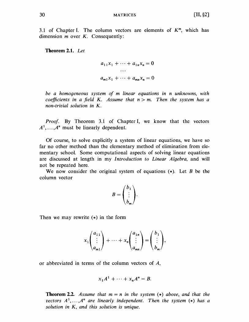
30 MATRICES [II, §2]
3.1 of Chapter I. The column vectors are elements of K m, which has
dimension mover K. Consequently:
Theorem 2.1. Let
be a homogeneous system of m linear equations in n unknowns, with coefficients in a field K. Assume that n > m. Then the system has a non-trivial solution in K.
Proof. By Theorem 3.1 of Chapter I, we know that the vectors A 1, ... ,An must be linearly dependent.
Of course, to solve explicitly a system of linear equations, we have so far no other method than the elementary method of elimination from elementary school. Some computational aspects of solving linear equations are discussed at length in my Introduction to Linear Algebra, and will not be repeated here.
We now consider the original system of equations (*). Let B be the column vector
Then we may rewrite (*) in the form
or abbreviated in terms of the column vectors of A,
Theorem 2.2. Assume that m = n in the system (*) above, and that the vectors A1, ... ,A n are linearly independent. T hen the system (*) has a solution in K, and this solution is unique.
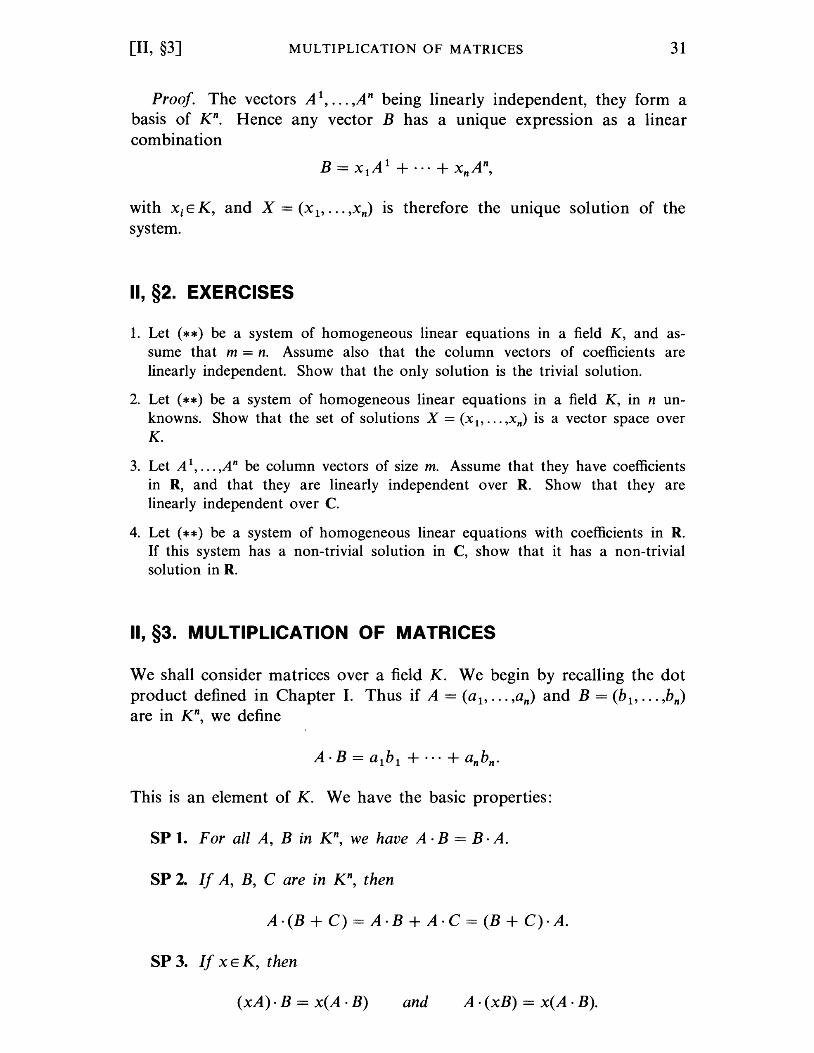
[II, §3] MULTIPLICATION OF MATRICES 31
Proof. The vectors AI, ... ,An being linearly independent, they form a basis of Kn. Hence any vector B has a unique expression as a linear combination
with Xi E K, and X = (x l' ... ,xn) is therefore the unIque solution of the system.
II, §2. EXERCISES
1. Let (**) be a system of homogeneous linear equations in a field K, and assume that m = n. Assume also that the column vectors of coefficients are linearly independent. Show that the only solution is the trivial solution.
2. Let (**) be a system of homogeneous linear equations in a field K, in n unknowns. Show that the set of solutions X = (x l' ... ,xn) is a vector space over K.
3. Let A 1, ... ,An be column vectors of size m. Assume that they have coefficients in R, and that they are linearly independent over R. Show that they are linearly independent over C.
4. Let (**) be a system of homogeneous linear equations with coefficients in R. If this system has a non-trivial solution in C, show that it has a non-trivial solution in R.
II, §3. MULTIPLICATION OF MATRICES
We shall consider matrices over a field K. We begin by recalling the dot product defined in Chapter I. Thus if A = (a 1, ••• ,an) and B = (b 1, ••• ,bn) are in K n
, we define
This is an element of K. We have the basic properties:
SP 1. For all A, B in K n, we have A· B = B· A.
SP 2. If A, B, C are in K n, then
A·(B + C) = A·B + A·C = (B + C)·A.
SP 3. If xEK, then
(xA) . B = x( A . B) and A . (xB) = x( A . B).
32 MATRICES [II, §3]
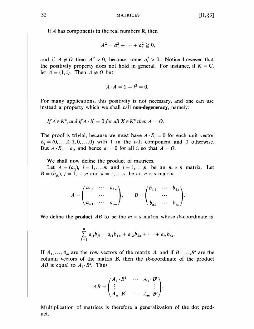
If A has components in the real numbers R, then
A 2 = ai + ... + a; > 0,
and if A =1= 0 then A2 > 0, because some af > 0. Notice however that the positivity property does not hold in general. F or instance, if K = C, let A = (1, i). Then A =1= 0 but
A . A = 1 + i2 = 0.
For many applications, this positivity is not necessary, and one can use instead a property which we shall call non-degeneracy, namely:
If AEKn, and if A·X = ° for all X EKn then A = o.
The proof is trivial, because we must have A· Ei = ° for each unit vector Ei = (0, ... ,0, 1, 0, ... ,0) with 1 in the i-th component and ° otherwise. But A· Ei = ai' and hence a i = ° for all i, so that A = o.
We shall now define the product of matrices. Let A = (aij), i = 1, ... ,m and j = 1, ... ,n, be an m x n matrix. Let
B = (b jk)' j = 1, ... ,n and k = 1, ... ,s, be an n x s matrix.
We define the product AB to be the m x s matrix whose ik-coordinate is
n
L aijbjk = ailblk + a i2 b 2k + ... + ainbnk · j= 1
If A l , ... ,Am are the row vectors of the matrix A, and if B l, ... ,Bs are the
column vectors of the matrix B, then the ik-coordinate of the product AB is equal to Ai· Bk. Thus
Multiplication of matrices is therefore a generalization of the dot product.
[II, §3] MULTIPLICATION OF MATRICES
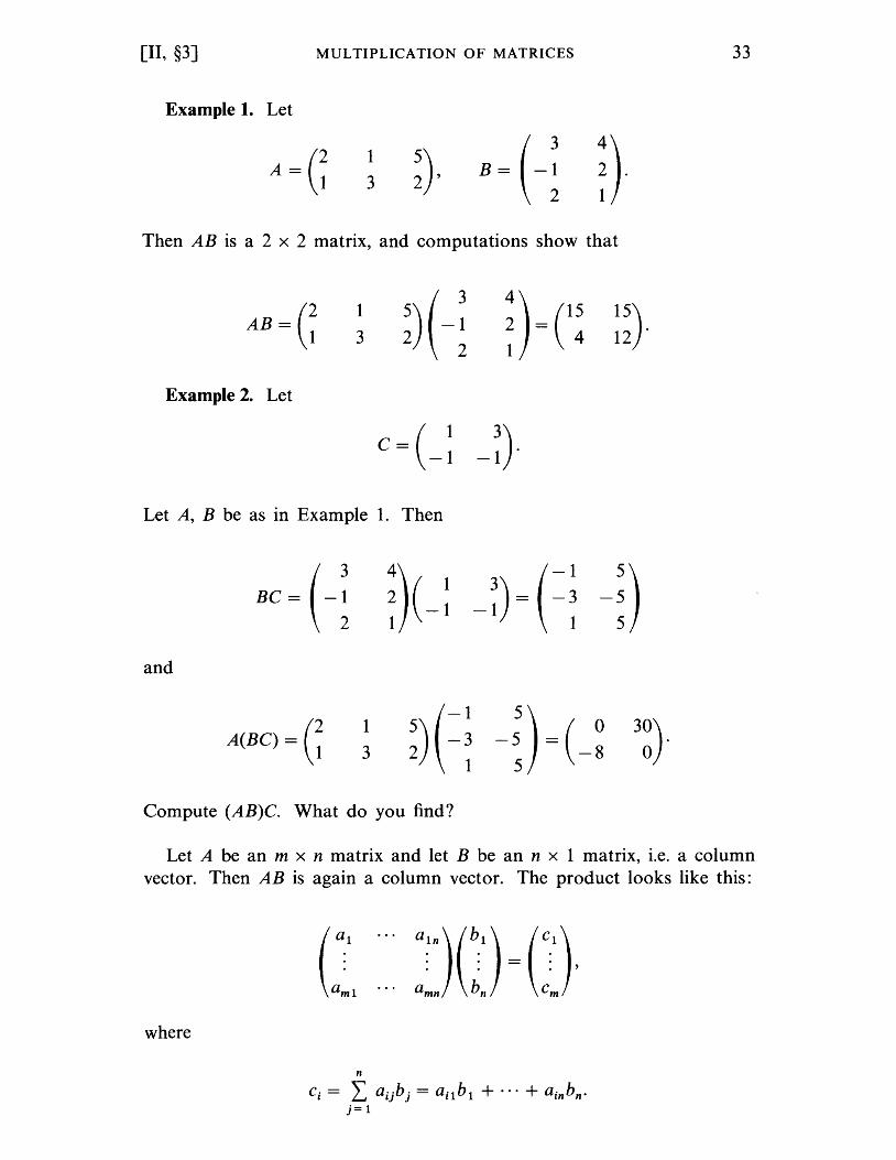
Example 1. Let
A=G 1
3 B=(-! ~). Then AB is a 2 x 2 matrix, and computations show that
AB=G 1 ~)( -! ~)=C! 3
Example 2. Let
C = ( 1 -1 -~).
Let A, B be as in Example 1. Then
and
A(BC) = G 1
3 (-1 5) ~) -~ -~ = (-~
Compute (AB)C. What do you find?
15) 12 .
3~)
33
Let A be an m x n matrix and let B be an n x 1 matrix, i.e. a column vector. Then AB is again a column vector. The product looks like this:
where
n
Ci = L aijb j = ai1b 1 + ... + ainbn· j= 1
34 MATRICES [II, §3]
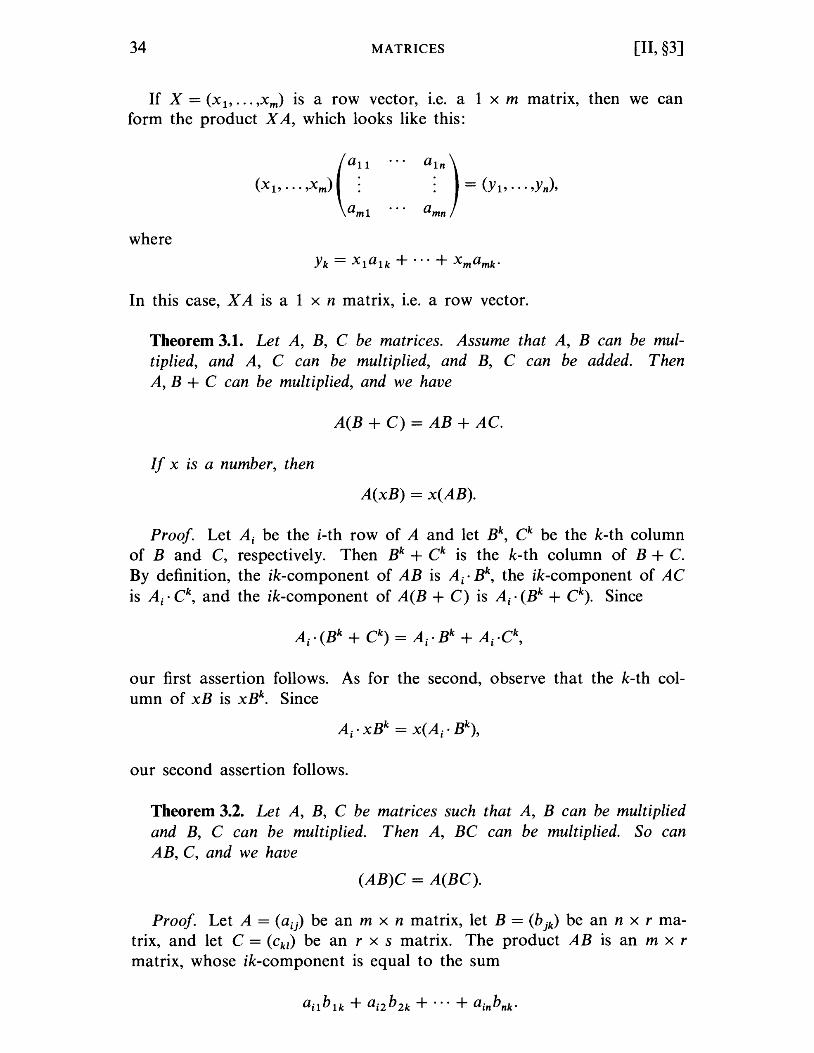
If X = (Xl' ... ,Xm) is a row vector, i.e. a 1 x m matrix, then we can form the product X A, which looks like this:
where
In this case, X A is a 1 x n matrix, i.e. a row vector.
Theorem 3.1. Let A, B, C be matrices. Assume that A, B can be multiplied, and A, C can be multiplied, and B, C can be added. Then A, B + C can be multiplied, and we have
A(B + C) = AB + AC.
If X is a number, then
A(xB) = x(AB).
Proof. Let Ai be the i-th row of A and let Bk, Ck be the k-th column of Band C, respectively. Then Bk + Ck is the k-th column of B + C. By definition, the ik-component of AB is Ai· Bk, the ik-component of AC is Ai· Ck, and the ik-component of A(B + C) is Ai· (Bk + Ck). Since
our first assertion follows. As for the second, observe that the k-th column of xB is XBk. Since
A.· XBk = x(A .. Bk) l l'
our second assertion follows.
Theorem 3.2. Let A, B, C be matrices such that A, B can be multiplied and B, C can be multiplied. Then A, BC can be multiplied. So can AB, C, and we have
(AB)C = A(BC).
Proof. Let A = (aij) be an m x n matrix, let B = (b jk) be an n x r matrix, and let C = (Ck1 ) be an r x s matrix. The product AB is an m x r matrix, whose ik-component is equal to the sum
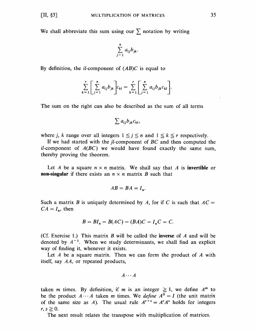
[II, §3] MULTIPLICATION OF MATRICES
We shall abbreviate this sum using our I notation by writing
n
I aijbjk · j= 1
By definition, the ii-component of (AB)C is equal to
The sum on the right can also be described as the sum of all terms
where j, k range over all integers 1 <j < nand 1 < k < r respectively.
35
If we had started with the jl-component of BC and then computed the ii-component of A(BC) we would have found exactly the same sum, thereby proving the theorem.
Let A be a square n x n matrix. We shall say that A is invertible or non-singular if there exists an n x n matrix B such that
Such a matrix B is uniquely determined by A, for if C is such that AC =
CA = In, then
B = BIn = B(AC) = (BA)C = InC = C.
(Cf. Exercise 1.) This matrix B will be called the inverse of A and will be denoted by A - 1. When we study determinants, we shall find an explicit way of finding it, whenever it exists.
Let A be a square matrix. Then we can form the product of A with itself, say AA, or repeated products,
A···A
taken m times. By definition, if m is an integer > 1, we define Am to be the product A··· A taken m times. We define AO = I (the unit matrix of the same size as A). The usual rule Ar+s = Ar AS holds for integers r, S > o.
The next result relates the transpose with multiplication of matrices.
36 MATRICES [II, §3]
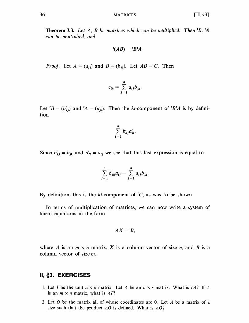
Theorem 3.3. Let A, B be matrices which can be multiplied. Then tB, tA can be multiplied, and
Proof. Let A = (a ij) and B = (b jk). Let AB = C. Then
n
Cik = L aijbjk · j=l
Let tB = (b~j) and tA = (ali). Then the ki-component of tBtA is by definition
n
L b~jali· j= 1
Since b~j = bjk and ali = aij we see that this last expression is equal to
n n
L bjkaij = L aijbjk · j=l j=l
By definition, this is the ki-component of tc, as was to be shown.
In terms of multiplication of matrices, we can now write a system of linear equations in the form
AX = B,
where A is an m x n matrix, X is a column vector of size n, and B is a column vector of size m.
II, §3. EXERCISES
1. Let I be the unit n x n matrix. Let A be an n x r matrix. What is I A? If A is an m x n matrix, what is AI?
2. Let D be the matrix all of whose coordinates are O. Let A be a matrix of a size such that the product AD is defined. What is AD?
[II, §3] MULTIPLICATION OF MATRICES
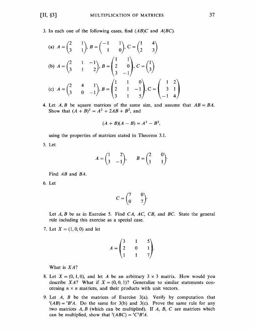
3. In each one of the following cases, find (AB)C and A(BC).
(a) A = G
(b) A = G
(c) A = G
~}B=(-~ ~}c=G
~ -~}B=O
~ _~}B=G
37
4. Let A, B be square matrices of the same size, and assume that AB = BA. Show that (A + B)2 = A2 + 2AB + B2, and
(A + B)(A - B) = A2 - B2,
using the properties of matrices stated in Theorem 3.1.
5. Let
Find AB and BA.
6. Let
Let A, B be as in Exercise 5. Find CA, AC, CB, and BC. State the general rule including this exercise as a special case.
7. Let X = (1, 0, 0) and let
What is XA?
1
° 1
8. Let X = (0,1,0), and let A be an arbitrary 3 x 3 matrix. How would you describe X A? What if X = (0,0, I)? Generalize to similar statements concerning n x n matrices, and their products with unit vectors.
9. Let A, B be the matrices of Exercise 3(a). Verify by computation that t(AB) = tBtA. Do the same for 3(b) and 3(c). Prove the same rule for any two matrices A, B (which can be multiplied). If A, B, C are matrices which can be multiplied, show that t(ABC) = tCtBtA.
38 MATRICES [II, §3]
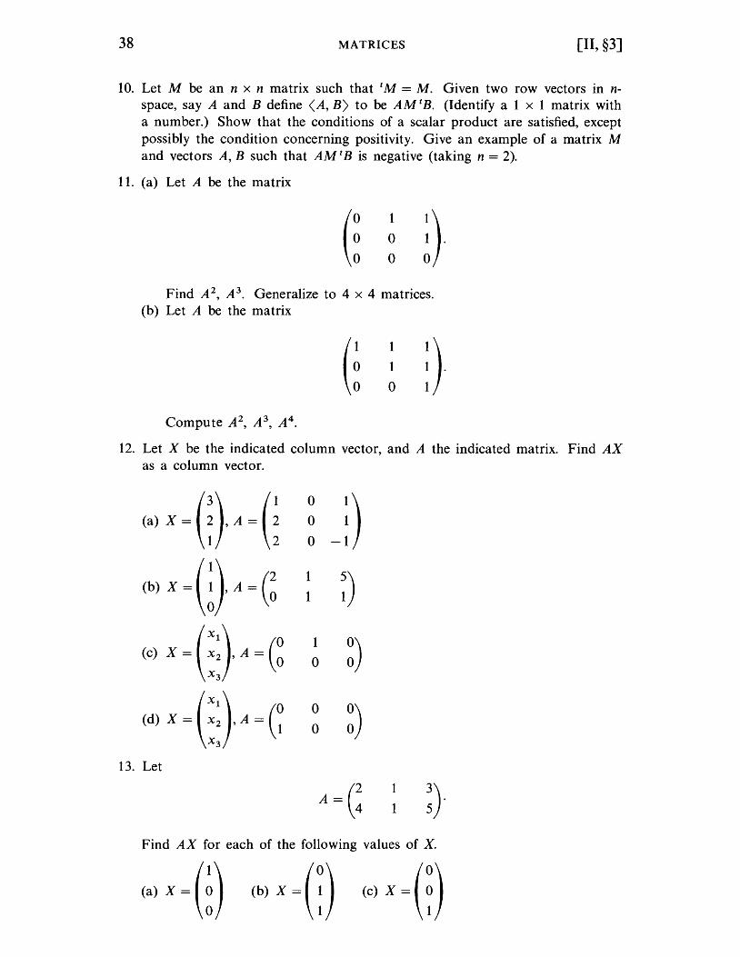
10. Let M be an n x n matrix such that tM = M. Given two row vectors in nspace, say A and B define (A, B) to be AM t B. (Identify a 1 x 1 matrix with a number.) Show that the conditions of a scalar product are satisfied, except possibly the condition concerning positivity. Give an example of a matrix M and vectors A, B such that AM t B is negative (taking n = 2).
11. (a) Let A be the matrix
1
o o
Find A 2, A3. Generalize to 4 x 4 matrices.
(b) Let A be the matrix
Compute A 2 , A 3 , A4.
1
1
o
12. Let X be the indicated column vector, and A the indicated matrix. Find AX as a column vector.
(a) X = G)' A = G 0
-D 0
0
(b) X=(~}A=G 1
~) 1
(c) X=(::}A=(~ 1 ~) 0
(d) X = (::) A = G 0 ~) 0
13. Let
A =(! 1
~} 1
Find AX for each of the following values of X.
(a) X=(~) (b) X=(!) (c) X=(D
[II, §3]
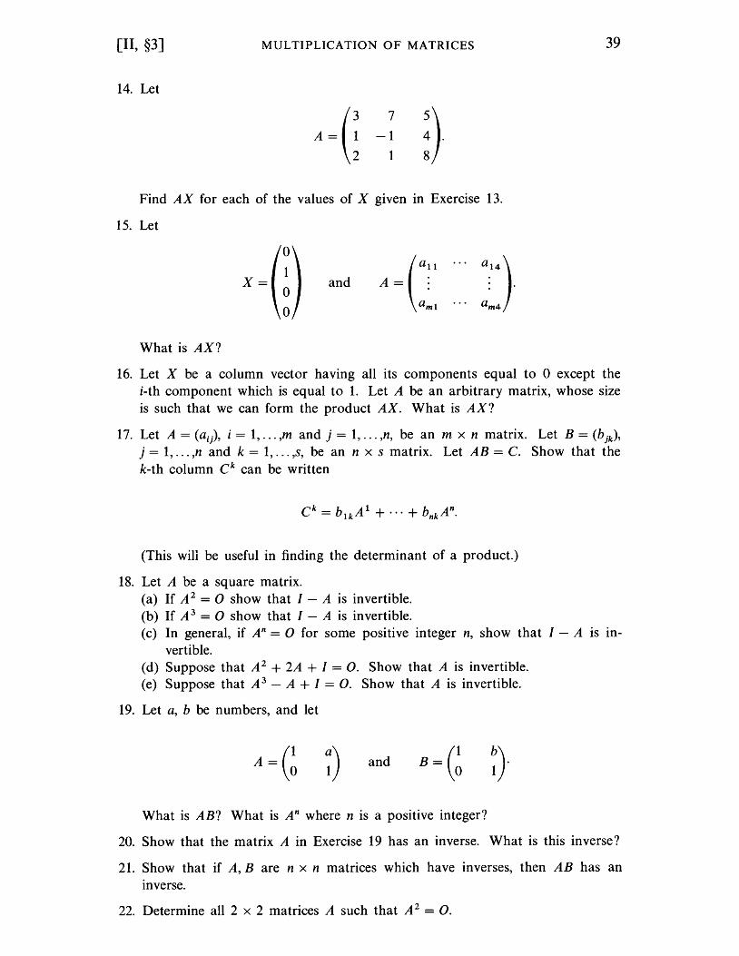
14. Let
MULTIPLICATION OF MATRICES
A=G 7
-1
1
Find AX for each of the values of X given in Exercise 13.
15. Let
and
What is AX?
39
16. Let X be a column vector having all its components equal to 0 except the i-th component which is equal to 1. Let A be an arbitrary matrix, whose size is such that we can form the product AX. What is AX?
17. Let A = (a i), i = 1, ... ,m and j = 1, ... ,n, be an m x n matrix. Let B = (b jk ),
j = 1, ... ,n and k = 1, ... ,s, be an n x s matrix. Let AB = C. Show that the k-th column C k can be written
(This win be useful in finding the determinant of a product.)
18. Let A be a square matrix. (a) If A 2 = 0 show that I - A is invertible. (b) If A 3 = 0 show that I - A is invertible. (c) In general, if An = 0 for some positive integer n, show that I - A is in
vertible. (d) Suppose that A 2 + 2A + I = o. Show that A is invertible. (e) Suppose that A 3 - A + I = o. Show that A is invertible.
19. Let a, b be numbers, and let
A=G ~) and B=G What is AB? What is An where n is a positive integer?
20. Show that the matrix A in Exercise 19 has an inverse. What is this inverse?
21. Show that if A, Bare n x n matrices which have inverses, then AB has an inverse.
22. Determine all 2 x 2 matrices A such that A 2 = o.
40
(
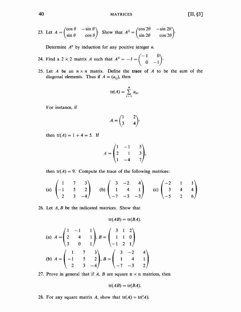
COS 8 23. Let A = . ()
sIn
MATRICES
- sin 8) 2 (COS 28 () . Show that A = . 2()
cos sIn
Determine An by induction for any positive integer n.
-sin 28). cos 2()
24. Find a 2 x 2 matrix A such that A2 = _/ = (-1 0). o -1
[II, §3]
25. Let A be an n x n matrix. Define the trace of A to be the sum of the diagonal elements. Thus if A = (a i)' then
n
tr(A) = L aii· i= 1
F or instance, if
A=G ~} then tr( A) = 1 + 4 = 5. If
A=G -1
1
-4
then tr(A) = 9. Compute the trace of the following matrices:
(a) (- ~ ~ ~) 2 3-4
-2 4) (-2 4 1 (c) 3
-3 -3 -5
26. Let A, B be the indicated matrices. Show that
tr(AB) = tr(BA).
(a) A =(: -1
~}B= ( ~ 1
n 4 1
0 1 -1 2
(b) A = ( -: 7
~} B = ( ~ -2
D 5 4
3 -4 -7 -3
27. Prove in general that if A, B are square n x n matrices, then
tr(AB) = tr(BA).
28. For any square matrix A, show that tr(A) = trCA).
4
2
[II, §3] MULTIPLICATION OF MATRICES 41
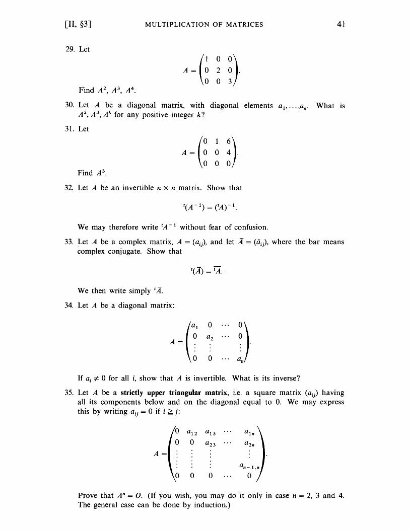
29. Let
(1 0 0)
A= 0 2 0 .
003
30. Let A be a diagonal matrix, with diagonal elements a 1, •.. ,an. What is A 2
, A 3, Ak for any positive integer k?
31. Let
(0 1 6)
A= 0 0 4 .
000 Find A3.
32. Let A be an invertible n x n matrix. Show that
We may therefore write tA -1 without fear of confusion.
33. Let A be a complex matrix, A = (a i), and let A = (aij)' where the bar means complex conjugate. Show that
We then write simply t A.
34. Let A be a diagonal matrix:
A=
If a i "# 0 for all i, show that A is invertible. What is its inverse?
35. Let A be a strictly upper triangular matrix, i.e. a square matrix (aij) having all its components below and on the diagonal equal to O. We may express this by writing aij = 0 if i ~ j:
o a 12 a 13 a 1n
o 0 a 23 a 2n
A=
o 0 o o
Prove that An = o. (If you wish, you may do it only in case n = 2, 3 and 4. The general case can be done by induction.)
42 MATRICES [II, §3]
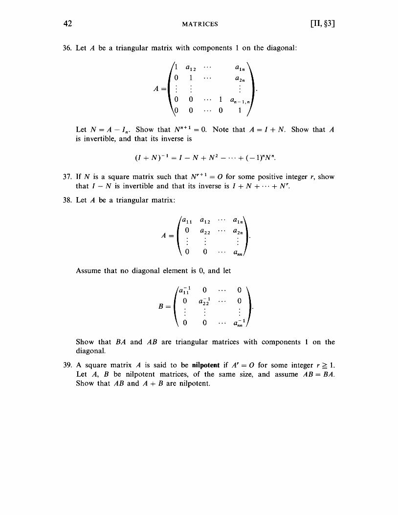
36. Let A be a triangular matrix with components 1 on the diagonal:
1 al2 aln
0 1 a2n
A= 0 0 1
0 0 0 1
Let N = A - In. Show that N n+ 1 = O. Note that A = I + N. Show that A is invertible, and that its inverse is
(I + N)-l = I - N + N 2 - ••• + (-l)"Nn.
37. If N is a square matrix such that N r + 1 = 0 for some positive integer r, show that I - N is invertible and that its inverse is I + N + ... + N r
•
38. Let A be a triangular matrix:
o
... a ln)
... a2n . .
ann
Assume that no diagonal element is 0, and let
o
B=
o
Show that BA and AB are triangular matrices with components 1 on the diagonal.
39. A square matrix A is said to be nilpotent if A r = 0 for some integer r ~ 1. Let A, B be nilpotent matrices, of the same size, and assume AB = BA. Show that AB and A + B are nilpotent.
CHAPTER III
Linear Mappings
We shall define the general notion of a mapping, which generalizes the notion of a function. Among mappings, the linear mappings are the most important. A good deal of mathematics is devoted to reducing questions concerning arbitrary mappings to linear mappings. For one thing, they are interesting in themselves, and many mappings are linear. On the other hand, it is often possible to approximate an arbitrary mapping by a linear one, whose study is much easier than the study of the original mapping. This is done in the calculus of several variables.
III, §1. MAPPINGS
Let S, S' be two sets. A mapping from S to S' is an association which to every element of S associates an element of S'. Instead of saying that F is a mapping from S into S', we shall often write the symbols F: S ---+ S'. A mapping will also be called a map, for the sake of brevity.
A function is a special type of mapping, namely it is a mapping from a set into the set of numbers, i.e. into R, or C, or into a field K.
We extend to mappings some of the terminology we have used for functions. For instance, if T: S ---+ S' is a mapping, and if u is an element of S, then we denote by T(u), or Tu, the element of S' associated to u by T. We call T(u) the value of T at u, or also the image of u under T. The symbols T(u) are read "T of u". The set of all elements T(u), when u ranges over all elements of S, is called the image of T. If W is a subset of S, then the set of elements T(w), when w ranges over all elements of W, is called the image of Wunder T, and is denoted by T(W).
44 LINEAR MAPPINGS [III,§I]
Let F: S ---+ Sf be a map from a set S into a set Sf. If x is an element of S, we often write
X 1---+ F(x)
with a special arrow 1---+ to denote the image of x under F. Thus, for instance, we would speak of the map F such that F(x) = x 2 as the map x 1---+ x 2
•
Example 1. Let S and Sf be both equal to R. Let f: R ---+ R be the function f(x) = x 2 (i.e. the function whose value at a number x is x 2 ). Then f is a mapping from R into R. Its image is the set of numbers > o.
Example 2. Let S be the set of numbers > 0, and let Sf = R. Let g: S ---+ Sf be the function such that g(x) = X
1/2
• Then g is a mapping from S into R.
Example 3. Let S be the set of functions having derivatives of all orders on the interval 0 < t < 1, and let Sf = S. Then the derivative D = d/dt is a mapping from S into S. Indeed, our map D associates the function df/dt = Df to the function f. According to our terminology, Df is the value of the mapping D at f.
Example 4. Let S be the set of continuous functions on the interval [0, 1] and let Sf be the set of differentiable functions on that interval. We shall define a mapping cI: S ---+ Sf by giving its value at any function f in S. Namely, we let clf (or cI(f)) be the function whose value at x is
(/f)(x) = s: f(t) dt.
Then cI(f) is differentiable function.
Example 5. Let S be the set R 3, i.e. the set of 3-tu pIes. Let A = (2,3, -1). Let L: R3 ---+ R be the mapping whose value at a vector X=(x,Y,z) is A·X. Then L(X)=A·X. If X=(I,I,-I), then the value of L at X is 6.
Just as we did with functions, we describe a mapping by giving its values. Thus, instead of making the statement in Example 5 describing the mapping L, we would also say: Let L: R3 ---+ R be the mapping L(X) = A . X. This is somewhat incorrect, but is briefer, and does not usually give rise to confusion. More correctly, we can write X 1---+ L(X) or X 1---+ A . X with the special arrow 1---+ to denote the effect of the map L on the element X.
[III, §1] MAPPINGS 45
Example 6. Let F: R2 --+ R2 be the mapping given by
F(x, y) = (2x, 2y).
Describe the image under F of the points lying on the circle x 2 + y2 = 1. Let (x, y) be a point on the circle of radius 1. Let u = 2x and v = 2y. Then u, v satisfy the relation
(U/2)2 + (V/2)2 = 1
or in other words,
Hence (u, v) is a point on the circle of radius 2. Therefore the image under F of the circle of radius 1 is a subset of the circle of radius 2. Conversely, given a point (u, v) such that
let x = u/2 and y = v/2. Then the point (x, y) satisfies the equation x2 + y2 = 1, and hence is a point on the circle of radius 1. Furthermore, F(x, y) = (u, v). Hence every point on the circle of radius 2 is the image of some point on the circle of radius 1. We conclude finally that the image of the circle of radius 1 under F is precisely the circle of radius 2.
Note. In general, let S, S' be two sets. To prove that S = S', one frequently proves that S is a subset of S' and that S' is a subset of S. This is what we did in the preceding argument.
Example 7. Let S be a set and let V be a vector space over the field K. Let F, G be mappings of S into V. We can define their sum F + G as the map whose value at an element t of S is F(t) + G(t). We also define the product of F by an element c of K to be the map whose value at an element t of S is cF(t). It is easy to verify that conditions VS 1 through VS 8 are satisfied.
Example 8. Let S be a set. Let F: S --+ K n be a mapping. For each element t of S, the value of F at t is a vector F(t). The coordinates of F(t) depend on t. Hence there are functions 11' ... ,In of S into K such that
F(t) = (11 (t), ... ,In(t)).
46 LINEAR MAPPINGS [III, §1]
These functions are called the coordinate functions of F. For instance, if K = R and if S is an interval of real numbers, which we denote by J, then a map
is also called a (parametric) curve in n-space.
Let S be an arbitrary set again, and let F, G: S ---+ K n be mappings of S into Kn. Let 11' ... ,In be the coordinate functions of F, and g1'.·· ,gn the coordinate functions of G. Then G(t) = (g 1 (t), ... ,gn(t)) for all t E S. Furthermore,
(F + G)(t) = F(t) + G(t) = (/1(t) + g1(t), ... ,In(t) + gn(t)),
and for any c E K,
(cF)(t) = cF(t) = (C!1(t), ... ,cln(t)).
We see in particular that the coordinate functions of F + G are.
Example 9. We can define a map F: R ---+ Rn by the association
Thus F(t) = (2t, lOt, t 3), and F(2) = (4, 100, 8). The coordinate functions of F are the functions 11,/2'!3 such that
!1(t) = 2t, and
Let U, V, W be sets. Let F: U ---+ V and G: V ---+ W be mappings. Then we can form the composite mapping from U into W, denoted by G 0 F. It is by definition the mapping defined by
(G 0 F)(t) = G(F(t))
for all t E U. If I: R ---+ R is a function and g: R ---+ R is also a function, then go I is the composite function.
[III, §1] MAPPINGS 47
The following statement is an important property of mappings.
Let U, V, W, S be sets. Let
F: U ---+ V, G: V ---+ W, and H:W---+S
be mappings. Then
Ho(GoF) = (HoG)oF.
Proof. Here again, the proof is very simple. By definition, we have, for any element u of U:
(H 0 (G 0 F))(u) = H((G 0 F)(u)) = H( G(F(u))).
On the other hand,
((H 0 G) 0 F)(u) = (H 0 G)(F(u)) = H( G(F(u))).
By definition, this means that
H 0 (G 0 F) = (H 0 G) 0 F.
We shall discuss inverse mappings, but before that, we need to mention two special properties which a mapping may have. Let
f: S ---+ S'
be a map. We say that f is injective if whenever x, YES and x =1= y, then f(x) =1= fey). In other words, f is injective means that f takes on distinct values at distinct elements of S. Put another way, we can say that f is injective if and only if, given x, YES,
f(x) = fey) implies x = y.
Example 10. The function
f: R---+R
such that f(x) = x 2 is not injective, because f(l) = f( -1) = 1. Also the function x ~ sin x is not injective, because sin x = sin(x + 2n). However, the map f: R ---+ R such that f(x) = x + 1 is injective, because if x + 1 = y + 1 then x = y.
48 LINEAR MAPPINGS [III, §1]
Again, let f: S ---+ S' be a mapping. We shall say that f is surjective if the image of f is all of S'.
The map
f: R ---+ R
such that f(x) = x 2 is not surjective, because its image consists of all numbers > 0, and this image is not equal to all of R. On the other hand, the map of R into R given by x ~ x 3 is surjective, because given a number y there exists a number x such that y = x 3 (the cube root of y). Thus every number is in the image of our map.
A map which is both injective and surjective is defined to be bijective. Let R + be the set of real numbers > O. As a matter of convention,
we agree to distinguish between the maps
and
given by the same formula x ~ x 2• The point is that when we view the
association x ~ x 2 as a map of R into R, then it is not surjective, and it is not injective. But when we view this formula as defining a map from R + into R +, then it gives both an injective and surjective map of R +
into itself, because every positive number has a positive square root, and such a positive square root is uniquely determined.
In general, when dealing with a map f: S ---+ S', we must therefore always specify the sets Sand S', to be able to say that f is injective, or surjective, or neither. To have a completely accurate notation, we should write
fs,s'
or some such symbol which specifies Sand S' into the notation, but this becomes too clumsy, and we prefer to use the context to make our meaning clear.
If S is any set, the identity mapping Isis defined to be the map such that I s(x) = x for all XES. We note that the identity map is both injective and surjective. If we do not need to specify the reference to S (because it is made clear by the context), then we write I instead of Is. Thus we have I(x) = x for all XES. We sometimes denote Is by ids or simply ide
Finally, we define inverse mappings. Let F: S ---+ S' be a mapping from one set into another set. We say that F has an inverse if there exists a mapping G: S' ---+ S such that
Go F = Is and
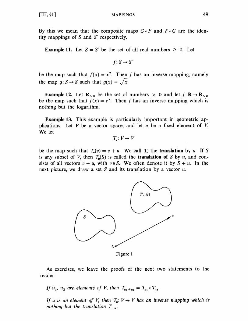
[III, §1] MAPPINGS 49
By this we mean that the composite maps G 0 F and FoG are the identity mappings of Sand S' respectively.
Example 11. Let S = S' be the set of all real numbers > O. Let
f: S --+ S'
be the map such that f(x) = x 2• Then f has an inverse mapping, namely
the map g: S --+ S such that g(x) = Jx,.
Example 12. Let R>o be the set of numbers > 0 and let f: R --+ R>o be the map such that f(x) = eX. Then f has an inverse mapping which is nothing but the logarithm.
Example 13. This example is particularly important in geometric applications. Let V be a vector space, and let u be a fixed element of V. We let
~: V--+ V
be the map such that ~(v) = v + u. We call ~ the translation by u. If S is any subset of V, then Tu(S) is called the translation of S by u, and consists of all vectors v + u, with v E S. We often denote it by S + u. In the next picture, we draw a set S and its translation by a vector u.
s u
o Figure 1
As exerCIses, we leave the proofs of the next two statements to the reader:
If u1, U 2 are elements of V, then ~1 +U2 = ~1 0 ~2·
If u is an element of V, then ~: V --+ V has an inverse mapping which is nothing but the translation T - U.
50 LINEAR MAPPINGS [III, §1]
Next, we have:
Let f:S~S'
be a map which has an inverse mapping g. Then f is both injective and surjective, that is f is bijective.
Proof. Let x, yE S. Let g: S' ~ S be the Inverse mappIng of f. If f(x) = f(y), then we must have
x = g(f(x) = g(f(y) = y,
and therefore f is injective. To prove that f is surjective, let z E S'. Then
f(g(z) = z
by definition of the inverse mapping, and hence z = f(x), where x = g(z). This proves that f is surjective.
The converse of the statement we just proved is also true, namely:
Let f: S ~ S' be a map which is bijective. Then f has an inverse mapping.
Proof. Given z E S', since f is surjective, there exists XES such that f(x) = z. Since f is injective, this element x is uniquely determined by z, and we can therefore define
g(z) = x.
By definition of g, we find that f(g(z) = z, and g(f(x) = x, so that g is an inverse mapping for f.
Thus we can say that a map f: S ~ S' has an inverse mapping if and only if f is bijective.
III, §1. EXERCISES
1. In Example 3, give Df as a function of x when f is the function: (a) f(x) = sin x (b) f(x) = eX (c) f(x) = log x
2. Prove the statement about translations in Example 13.
3. In Example 5, give L(X) when X is the vector: (a) (1, 2, - 3) (b) (-1, 5, 0) (c) (2, 1, 1)
[III, §2] LINEAR MAPPINGS 51
4. Let F: R --+ R2 be the mapping such that F(t) = (e t, t). What is F(l), F(O),
F( -I)?
5. Let G: R --+ R2 be the mapping such that G(t) = (t, 2t). Let F be as in Exercise 4. What is (F + G)(l), (F + G)(2), (F + G)(O)?
6. Let F be as in Exercise 4. What is (2F)(O), (nF)(l)?
7. Let A = (1, 1, -1, 3). Let F: R4 --+ R be the mapping such that for any vector X = (Xl' x 2 ' x 3 , x 4 ) we have F(X) = X . A + 2. What is the value of F(X) when (a) X = (1,1,0, -1) and (b) X = (2, 3, -1, I)?
In Exercises 8 through 12, refer to Example 6. In each case, to prove that the image is equal to a certain set S, you must prove that the image is contained in S, and also that every element of S is in the image.
8. Let F: R2 --+ R2 be the mapping defined by F(x, y) = (2x, 3y). Describe the image of the points lying on the circle x 2 + y2 = 1.
9. Let F: R2 --+ R2 be the mapping defined by F(x, y) = (xy, y). Describe the image under F of the straight line X = 2.
10. Let F be the mapping defined by F(x, y) = (eX cos y, eX sin y). Describe the image under F of the line X = 1. Describe more generally the image under F of a line X = c, where c is a constant.
11. Let F be the mapping defined by F(t, u) = (cos t, sin t, u). Describe geometrically the image of the (t, u)-plane under F.
12. Let F be the mapping defined by F(x, y) = (x13, xI4). What is the image under F of the ellipse
III, §2. LINEAR MAPPINGS
x2 y2 -+-=1? 9 16 .
Let V, V' be the vector spaces over the field K. A linear mapping
F:V~V'
is a mapping which satisfies the following two properties.
LM 1. For any elements u, v in V we have
F(u + v) = F(u) + F(v).
LM 2. For all c in K and v in V we have
F(cv) = cF(v).
52 LINEAR MAPPINGS [III, §2]
If we wish to specify the field K, we also say that F is K-linear. Since we usually deal with a fixed field K, we omit the prefix K, and say sim pI y that F is linear.
Example 1. Let V be a finite dimensional space over K, and let {V1' ... ,vn } be a basis of V. We define a map
by associating to each element v E V its coordinate vector X with respect to the basis. Thus if
We assert that F is a linear map. If
with coordinate vector Y = (Yl'··· ,Yn), then
whence F(v + w) = X + Y = F(v) + F(w). If cEK, then
and hence F(cv) = cX = cF(v). This proves that F is linear.
Example 2. Let V = R3 be the vector space (over R) of vectors in 3-space. Let V' = R2 be the vector space of vectors in 2-space. We can define a mapping
by the projection, namely F(x, y, z) = (x, y). We leave it to you to check that the conditions LM 1 and LM 2 are satisfied.
More generally, let r, n be positive integers, r < n. Then we have a projection mapping
defined by the rule
It is trivially verified that this map is linear.
[III, §2] LINEAR MAPPINGS 53
Example 3. Let A = (1,2, -1). Let V = R3 and V' = R. We can define a mapping L = LA: R 3 ~ R by the association X ~ X . A, i.e.
L(X) = X·A
for any vector X in 3-space. The fact that L is linear summarizes two known properties of the scalar product, namely, for any vectors X, Y in R3 we have
(X + Y)·A = X·A + Y·A,
(cX)·A = c(X·A).
More generally, let K be a field, and A a fixed vector in Kn. We have a linear map (Le. K-linear map)
such that LA(X) = X· A for all X E Kn. We can even generalize this to matrices. Let A be an m x n matrix in
a field K. We obtain a linear map
such that
for every column vector X in Kn. Again the linearity follows from properties of multiplication of matrices. If A = (aij) then AX looks like this:
This type of multiplication will be met frequently in the sequel.
Example 4. Let V be any vector space. The mapping which associates to any element u of V this element itself is obviously a linear mapping, which is called the identity mapping. We denote it by id or simply I. Thus id(u) = u.
Example 5. Let V, V' be any vector spaces over the field K. The mapping which associates the element 0 in V'to any element u of V is called the zero mapping and is obviously linear. It is also denoted by O.
54 LINEAR MAPPINGS [III, §2]
As an exercise (Exercise 2) prove:
Let L: V ~ W be a linear map. Then L(O) = O.
In particular, if F: V ~ W is a mapping and F(O) 1= 0 then F is not lin ear.
Example 6. The space of linear maps. Let V, V' be two vector spaces over the field K. We consider the set of all linear mappings from V into V', and denote this set by .P(V, V'), or simply .P if the reference to V, V' is clear. We shall define the addition of linear mappings and their multiplication by numbers in such a way as to make .P into a vector space.
Let T: V ~ V' and F: V ~ V' be two linear mappings. We define their sum T + F to be the map whose value at an element u of V is T(u) + F(u). Thus we may write
(T + F)(u) = T(u) + F(u).
The map T + F is then a linear map. Indeed, it is easy to verify that the two conditions which define a linear map are satisfied. For any elements u, v of V, we have
(T + F)(u + v) = T(u + v) + F(u + v)
Furthermore, if C E K, then
= T(u) + T(v) + F(u) + F(v)
= T(u) + F(u) + T(v) + F(v)
= (T + F)(u) + (T + F)(v).
(T + F)(cu) = T(cu) + F(cu)
= cT(u) + cF(u)
= c[T(u) + F(u)]
= c[(T + F)(u)].
Hence T + F is a linear map. If a E K, and T: V ~ V' is a linear map, we define a map aT from V
into V' by giving its value at an element u of V, namely (aT)(u) = aT(u). Then it is easily verified that aT is a linear map. We leave this as an exerCIse.
We have just defined operations of addition and scalar multiplication in our set!l'. Furthermore, if T: V ~ V' is a linear map, i.e. an element of !l', then we can define - T to be (- 1) T, i.e. the product of the
[III, §2] LINEAR MAPPINGS 55
number - 1 by T. Finally, we have the zero-map, which to every element of V associates the element 0 of V'. Then !l' is a vector space. In other words, the set of linear maps from V into V'is itself a vector space. The verification that the rules VS 1 through VS 8 for a vector space are satisfied is easy and left to the reader.
Example 7. Let V = V' be the vector space of real valued functions of a real variable which have derivatives of all order. Let D be the derivative. Then D: V ~ V is a linear map. This is merely a brief way of summarizing known properties of the derivative, namely
D(f + g) = Df + Dg, and D(cf) = cDf
for any differentiable functions f, g and constant c. If f is in V, and I is the identity map, then
(D + I)f = Df + f·
Thus when f is the function such that f(x) = eX then (D + I)f is the function whose value at x is eX + eX = 2e X.
If f(x) = sin x, then (D + I)f)(x) = cos x + sin x.
Let T: V ~ V' be a linear mapping. Let u, v, w be elements of V. Then
T(u + v + w) = T(u) + T(v) + T(w).
This can be seen stepwise, using the definition of linear mappings. Thus
T(u + v + w) = T(u + v) + T(w) = T(u) + T(v) + T(w).
Similarly, given a sum of more than three elements, an analogous property is satisfied. For instance, let u I' ... ,Un be elements of V. Then
The sum on the right can be taken in any order. A formal proof can easily be given by induction, and we omit it.
If aI' ... ,an are numbers, then
We show this for three elements.
T(alu + a2 v + a3 w) = T(aIu) + T(a 2 v) + T(a 3 w)
= al T(u) + a2 T(v) + a3 T(w).
56 LINEAR MAPPINGS [III, §2]
The next theorem will show us how a linear map is determined when we know its value on basis elements.
Theorem 2.1. Let V and W be vector spaces. Let {v l' ... ,vn} be a basis of V, and let W l , ... ,Wn be arbitrary elements of W Then there exists a unique linear mapping T: V ~ W such that
If Xl' ... ,Xn are numbers, then
T(X1Vl + ... + XnVn) = X1W l + ... + XnWn·
Proof. We shall prove that a linear map T satisfying the required conditions exists. Let v be an element of V, and let Xl' ... ,xn be the unique numbers such that v = X1V l + ... + xnvn. We let
We then have defined a mapping T from V into W, and we contend that T is linear. If v'is an element of V, and if v' = Y1V l + ... + Ynvn, then
By definition, we obtain
= T(v) + T(V').
Let c be a number. Then cv = CX1V l + ... + CXnVn' and hence
T(cv) = CX1W l + ... + cXnwn = cT(v).
We have therefore proved that T is linear, and hence that there exists a linear map as asserted in the theorem.
Such a map is unique, because for any element X1V l + ... + XnVn of V, any linear map F: V ~ W such that F(v i) = Wi (i = 1, ... ,n) must also satisfy
This concludes the proof.
[III, §2] LINEAR MAPPINGS
III, §2. EXERCISES
1. Determine which of the following mappings F are linear. (a) F: R3 ~ R2 defined by F(x, y, z) = (x, z) (b) F: R4 ~ R4 defined by F(X) = -x (c) F: R3 ~ R3 defined by F(X) = X + (0, -1, 0) (d) F: R2 ~ R2 defined by F(x, y) = (2x + y, y) (e) F: R2 ~ R2 defined by F(x, y) = (2x, y - x) (f) F: R2 ~ R2 defined by F(x, y) = (y, x) (g) F: R2 ~ R defined by F(x, y) = xy
57
(h) Let U be an open subset of R3, and let V be the vector space of dif
feren tiable functions on U. Let V' be the vector space of vector fields on U. Then grad: V ~ V'is a mapping. Is it linear? (For this part (h) we assume you know some calculus.)
2. Let T: V ~ W be a linear map from one vector space into another. Show that T(O) = o.
3. Let T: V ~ W be a linear map. Let u, v be elements of V, and let Tu = w. If Tv = 0, show that T(u + v) is also equal to w.
4. Let T: V ~ W be a linear map. Let U be the subset of elements u EV such that T(u) = o. Let WE Wand suppose there is some element Vo E V such that T(vo) = w. Show that the set of elements v E V satisfying T(v) = w is precisely Vo + U.
5. Let T: V ~ W be a linear map. Let v be an element of V. Show that T(-v) = -T(v).
6. Let V be a vector space, and f: V ~ R, g: V ~ R two linear mappings. Let F: V ~ R2 be the mapping defined by F(v) = (f(v), g(v). Show that F is linear. Generalize.
7. Let V, W be two vector spaces and let F: V ~ W be a linear map. Let U be the subset of V consisting of all elements v such that F(v) = o. Prove that U is a subspace of V.
8. Which of the mappings in Exercises 4, 7, 8, 9, of §1 are linear?
9. Let V be a vector space over R, and let v, WE V. The line passing through v and parallel to W is defined to be the set of all elements v + tw with t E R. The line segment between v and v + w is defined to be the set of all elements
v + tw with 0 ~ t ~ 1.
Let L: V ~ U be a linear map. Show that the image under L of a line segment in V is a line segment in U. Between what points?
Show that the image of a line under L is either a line or a point.
Let V be a vector space, and let Vi' v2 be two elements of V which are linearly independent. The set of elements of V which can be written in the
58 LINEAR MAPPINGS [III, §2]
and
is called the parallelogram spanned by V1' v2 •
10. Let V and W be vector spaces, and let F: V ~ W be a linear map. Let V 1, V2
be linearly independent elements of V, and assume that F( v 1)' F( v2 ) are linearly independent. Show that the image under F of the parallelogram spanned by V 1 and V 2 is the parallelogram spanned by F(v 1), F(v2 ).
11. Let F be a linear map from R 2 in to itself such that
and F(E2 ) = (-1, 2).
Let S be the square whose corners are at (0,0), (1, 0), (1, 1), and (0, 1). Show that the image of this square under F is a parallelogram.
12. Let A, B be two non-zero vectors in the plane such that there is no constant c#-O such that B = cA. Let T be a linear mapping of the plane into itself such that T(E 1) = A and T(E 2 ) = B. Describe the image under T of the rectangle whose corners are (0, 1), (3, 0), (0, 0), and (3, 1).
13. Let A, B be two non-zero vectors in the plane such that there is no constant c#-O such that B = cA. Describe geometrically the set of points tA + uB for values of t and u such that 0 ~ t ~ 5 and 0 ~ u ~ 2.
14. Let Tu: V ~ V be the translation by a vector u. For which vectors u is Tu a linear map? Proof?
15. Let V, W be two vector spaces, and F: V ~ W a linear map. Let W 1, ... ,Wn be elements of W which are linearly independent, and let v 1 , ••• ,Vn be elements of V such that F(vi ) = Wi for i = 1, ... ,no Show that v1 , ••• ,vn are linearly independent.
16. Let V be a vector space and F: V ~ R a linear map. Let W be the subset of V consisting of all elements v such that F(v) = O. Assume that W #- V, and let Vo be an element of V which does not lie in W. Show that every element of V can be written as a sum W + cVo, with some W in Wand some number c.
17. In Exercise 16, show that W is a subspace of V. Let {v 1 , ••• ,vn} be a basis of W. Show that {vo, v1, ... ,vn} is a basis of V.
18. Let L: R2 ~ R2 be a linear map, having the following effect on the indicated vectors: (a) L(3, 1) = (1, 2) and L( -1, 0) = (1, 1) (b) L(4, 1) = (1, 1) and L(l, 1) = (3, -2) (c) L(l, 1) = (2, 1) and L( -1, 1) = (6, 3). In each case compute L (1, 0).
19. Let L be as in (a), (b), (c), of Exercise 18. Find L(O, 1).
[III, §3] THE KERNEL AND IMAGE OF A LINEAR MAP 59
III, §3. THE KERNEL AND IMAGE OF A LINEAR MAP
Let V, W be vector spaces over K, and let F: V ~ W be a linear map. We define the kernel of F to be the set of elements v E V such that F(v) = o.
We denote the kernel of F by Ker F.
Example 1. Let L: R3 ~ R be the map such that
L(x, y, z) = 3x - 2y + z.
Thus if A = (3, - 2, 1), then we can write
L(X) = X·A = A·X.
Then the kernel of L is the set of solutions of the equation
3x - 2y + z = 0.
Of course, this generalizes to n-space. If A is an arbitrary vector in Rn,
we can define the linear map
such that LA(X) = A· X. Its kernel can be interpreted as the set of all X which are perpendicular to A.
Example 2. Let P: R3 ~ R2 be the projection, such that
P(x, y, z) = (x, y).
Then P is a linear map whose kernel consists of all vectors in R3 whose first two coordinates are equal to 0, i.e. all vectors
(0, 0, z)
with arbitrary component z.
We shall now prove that the kernel of a linear map F: V ~ W is a subspace of V. Since F( 0) = 0, we see that 0 is in the kernel. Let v, w
be in the kernel. Then F(v + w) = F(v) + F(w) = 0 + 0 = 0, so that v + w is in the kernel. If e is a number, then F(ev) = eF(v) = 0 so that ev is also in the kernel. Hence the kernel is a subspace.
60 LINEAR MAPPINGS [III, §3]
The kernel of a linear map is useful to determine when the map is injective. Namely, let F: V ~ W be a linear map. We contend that following two conditions are equivalent:
1. The kernel of F is equal to {o}.
2. If v, ware elements of V such that F(v) = F(w), then v = w. In other words, F is injective.
To prove our contention, assume first that Ker F = {O}, and suppose that v, ware such that F(v) = F(w). Then
F(v - w) = F(v) - F(w) = O.
By assumption, v - w = 0, and hence v = w. Conversely, assume that F is injective. If v is such that
F(v) = F(O) = 0,
we conclude that v = o.
The kernel of F is also useful to describe the set of all elements of V which have a given image in Wunder F. We refer the reader to Exercise 4 for this.
Theorem 3.1. Let F: V ~ W be a linear map whose kernel is {Ole If v l , ... ,Vn are linearly independent elements of V, then F(v l ), ... ,F(vn) are linearly independent elements of W.
Proof. Let Xl' ... ,xn be numbers such that
By linearity, we get
Hence XlVl + ... + XnVn = O. Since v l , ... ,Vn are linearly independent, it follows that Xi = 0 for i = 1, ... ,no This proves our theorem.
Let F: V ~ W be a linear map. The image of F is the set of elements w in W such that there exists an element of v of V such that F(v) = w.
The image of F is a subspace of W.
[III, §3] THE KERNEL AND IMAGE OF A LINEAR MAP 61
To prove this, observe first that F(O) = 0, and hence 0 is in the image. Next, suppose that WI' W2 are in the image. Then there exist elements VI' v2 of V such that F(v l ) = WI and F(v2 ) = W 2 • Hence
thereby proving that WI + W2 is in the image. If c is a number, then
Hence CW I is in the image. This proves that the image is a subspace of W.
We denote the image of F by 1m F.
The next theorem relates the dimensions of the kernel and image of a linear map with the dimension of the space on which the map is defined.
Theorem 3.2. Let V be a vector space. Let L: V ~ W be a linear map of V into another space W. Let n be the dimension of V, q the dimension of the kernel of L, and s the dimension of the image of L. Then n = q + s. In other words,
dim V = dim Ker L + dim 1m L.
Proof. If the image of L consists of 0 only, then our assertion is trivial. We may therefore assume that s > O. Let {wI, ... ,ws} be a basis of the image of L. Let VI' ••• ,vs be elements of V such that L(vi) = Wi for i = 1, ... ,so If the kernel of L is not {O}, let {u I , ... ,uq } be a basis of the kernel. If the kernel is { O}, it is understood that all reference to {u l , ... ,uq } is to be omitted in what follows. We contend that {VI' ••• 'vs ' U I , ... ,uq } is a basis of V. This will suffice to prove our assertion. Let V be any element of V. Then there exist numbers Xl' ... ,xs such that
because {WI' ... ,Ws } is a basis of the image of L. By linearity,
and again by linearity, subtracting the right-hand side from the left-hand side, it follows that
62 LINEAR MAPPINGS [III, §3]
Hence v - XlVl - ... - XsVs lies in the kernel of L, and there exist numbers Yl' ... ,Yq such that
Hence
is a linear combination of v l , ... ,vs'u l , ... ,uq • This proves that these s + q elements of V generate V.
We now show that they are linearly independent, and hence that they constitute a basis. Suppose that there exists a linear relation:
Applying L to this relation, and using the fact that L(uj ) = 0 for j = 1, ... ,q, we obtain
But L(v l ), ... ,L(vs) are none other than wl , ..• 'ws' which have been assumed linearly independent. Hence Xi = 0 for i = 1, ... ,so Hence
But U l , ... ,uq constitute a basis of the kernel of L, and in particular, are linearly independent. Hence all Yj = 0 for j = 1, ... ,q. This concludes the proof of our assertion.
Example 1 (Cont.). The linear map L: R3 --+ R of Example 1 IS given by the formula
L(x, y, z) = 3x - 2y + z.
Its kernel consists of all solutions of the equation
3x - 2y + z = o.
Its image is a subspace of R, is not {O}, and hence consists of all of R. Thus its image has dimension 1. Hence its kernel has dimension 2.
Example 2 (Cont.). The projection P: R3 --+ R2 of Example 2 is obviously surjective, and its kernel has dimension 1.
In Chapter V, §3 we shall investigate in general the dimension of the space of solutions of a system of homogeneous linear equations.
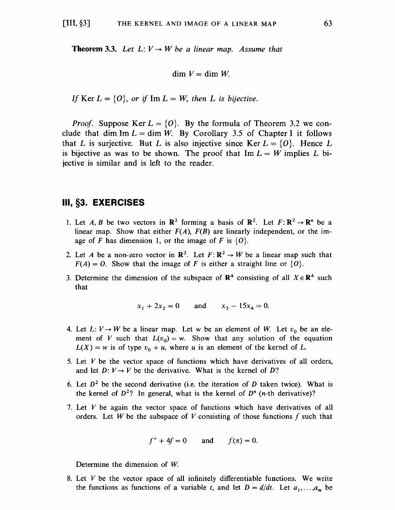
[III, §3] THE KERNEL AND IMAGE OF A LINEAR MAP 63
Theorem 3.3. Let L: V --+ W be a linear map. Assume that
dim V= dim W
If Ker L = {O}, or if 1m L = W, then L is bijective.
Proof. Suppose Ker L = {O}. By the formula of Theorem 3.2 we conclude that dim 1m L = dim W By Corollary 3.5 of Chapter I it follows that L is surjective. But L is also injective since Ker L = {O}. Hence L is bijective as was to be shown. The proof that 1m L = W implies L bijective is similar and is left to the reader.
III, §3. EXERCISES
1. Let A, B be two vectors in R2 forming a basis of R2. Let F: R2 -+ Rn be a linear map. Show that either F(A), F(B) are linearly independent, or the image of F has dimension 1, or the image of F is {O}.
2. Let A be a non-zero vector in R2. Let F: R2 -+ W be a linear map such that F(A) = O. Show that the image of F is either a straight line or {O}.
3. Determine the dimension of the subspace of R4 consisting of all X E R4 such that
and
4. Let L: V -+ W be a linear map. Let w be an element of W. Let Vo be an element of V such that L(vo) = w. Show that any solution of the equation L(X) = w is of type Vo + u, where U is an element of the kernel of L.
5. Let V be the vector space of functions which have derivatives of all orders, and let D: V -+ V be the derivative. What is the kernel of D?
6. Let D2 be the second derivative (i.e. the iteration of D taken twice). What is the kernel of D2? In general, what is the kernel of Dn (n-th derivative)?
7. Let V be again the vector space of functions which have derivatives of all orders. Let W be the subspace of V consisting of those functions f such that
f" + 4f= 0 and f(n) = O.
Determine the dimension of W.
8. Let V be the vector space of all infinitely differentiable functions. We write the functions as functions of a variable t, and let D = d/dt. Let a1 , ••• ,am be
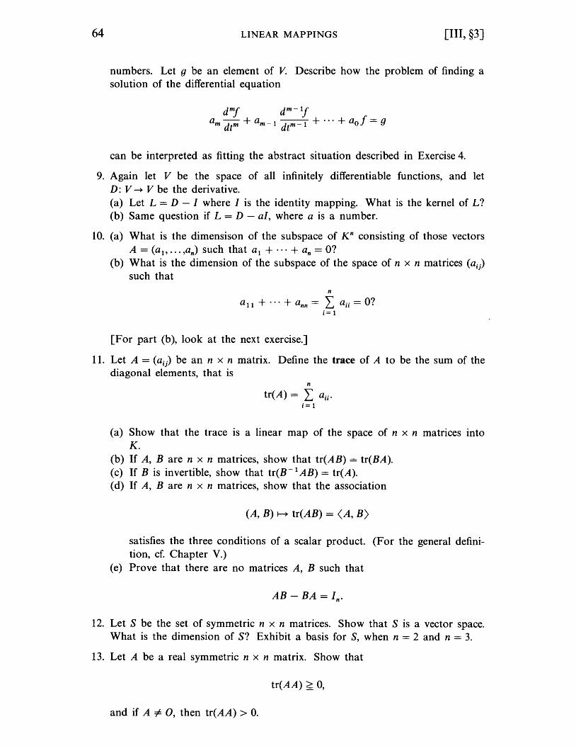
64 LINEAR MAPPINGS [III, §3]
numbers. Let g be an element of V. Describe how the problem of finding a solution of the differential equation
can be interpreted as fitting the abstract situation described in Exercise 4.
9. Again let V be the space of all infinitely differentiable functions, and let D: V -+ V be the derivative. (a) Let L = D - I where I is the identity mapping. What is the kernel of L? (b) Same question if L = D - aI, where a is a number.
10. (a) What is the dimensison of the subspace of K n consisting of those vectors A = (a 1, ••• ,an) such that a1 + ... + an = o?
(b) What is the dimension of the subspace of the space of n x n matrices (ai)
such that n
a 11 + ... + ann = L au = o? i= 1
[For part (b), look at the next exercise.]
11. Let A = (aij) be an n x n matrix. Define the trace of A to be the sum of the diagonal elements, that is
n
tr(A) = L au· i= 1
(a) Show that the trace is a linear map of the space of n x n matrices into K.
(b) If A, Bare n x n matrices, show that tr(AB) = tr(BA). (c) If B is invertible, show that tr(B- 1 AB) = tr(A). (d) If A, Bare n x n matrices, show that the association
(A, B) ~ tr(AB) = (A, B)
satisfies the three conditions of a scalar product. (For the general definition, cf. Chapter V.)
(e) Prove that there are no matrices A, B such that
AB - BA = In.
12. Let S be the set of symmetric n x n matrices. Show that S is a vector space. What is the dimension of S? Exhibit a basis for S, when n = 2 and n = 3.
13. Let A be a real symmetric n x n matrix. Show that
tr(AA) ~ 0,
and if A "# 0, then tr(AA) > O.
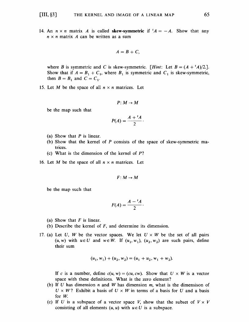
[III, §3] THE KERNEL AND IMAGE OF A LINEAR MAP 65
14. An n x n matrix A is called skew-symmetric if tA = -A. Show that any n x n matrix A can be written as a sum
A = B + C,
where B is symmetric and C is skew-symmetric. [Hint: Let B = (A + tA)j2.]. Show that if A = Bl + C l , where Bl is symmetric and C l is skew-symmetric, then B = Bl and C = Cl.
15. Let M be the space of all n x n matrices. Let
P:M-+M
be the map such that
A+tA P(A) = .
2
(a) Show that P is linear. (b) Show that the kernel of P consists of the space of skew-symmetric ma
trices. (c) What is the dimension of the kernel of P?
16. Let M be the space of all n x n matrices. Let
be the map such that
(a) Show that F is linear.
F:M-+M
A-tA F(A) = 2
(b) Describe the kernel of F, and determine its dimension.
17. (a) Let U, W be the vector spaces. We let U x W be the set of all pairs (u, w) with UE U and WE W If (u l , Wl)' (u 2 , w2 ) are such pairs, define their sum
If c is a number, define c(u, w) = (cu, cw). Show that U x W is a vector space with these definitions. What is the zero element?
(b) If U has dimension nand W has dimension m, what is the dimensison of U x W? Exhibit a basis of U x W in terms of a basis for U and a basis for W
(c) If U is a subspace of a vector space V, show that the subset of V x V consisting of all elements (u, u) with U E U is a subspace.
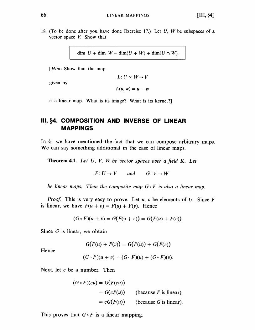
66 LINEAR MAPPINGS [III, §4]
18. (To be done after you have done Exercise 17.) Let U, W be subspaces of a vector space V. Show that
dim U + dim W = dim(U + W) + dim(U n W).
[Hint: Show that the map
L: U x W-+ V given by
L(u, w) = u - w
is a linear map. What is its image? What is its kernel?]
III, §4. COMPOSITION AND INVERSE OF LINEAR MAPPINGS
In §1 we have mentioned the fact that we can compose arbitrary maps. We can say something additional in the case of linear maps.
Theorem 4.1. Let U, V, W be vector spaces over a field K. Let
F: U --+ V and G: V--+ W
be linear maps. Then the composite map G 0 F is also a linear map.
Proof. This is very easy to prove. Let u, v be elements of U. Since F is linear, we have F(u + v) = F(u) + F(v). Hence
(G 0 F)(u + v) = G(F(u + v)) = G(F(u) + F(v)).
Since G is linear, we obtain
G(F(u) + F(v)) = G(F(u)) + G(F(v)) Hence
(G 0 F)(u + v) = (G 0 F)(u) + (G 0 F)(v).
Next, let c be a number. Then
(G 0 F)(cu) = G(F(cu))
= G(cF(u))
= cG(F(u))
(because F is linear)
(beca use G is linear).
This proves that Go F is a linear mapping.
[III, §4] COMPOSITION AND INVERSE OF LINEAR MAPPINGS 67
The next theorem states that some of the rules of arithmetic concerning the product and sum of numbers also apply to the composition and sum of linear mappings.
Theorem 4.2. Let U, V, W be vector spaces over a field K. Let
F:U~V
be a linear mapping, and let G, H be two linear mappings of V into W Then
(G + H)oF = GoF + HoF.
If c is a number, then
(cG)oF = c(GoF).
If T: U ~ V is a linear mapping from U into V, then
G 0 (F + T) = G 0 F + GoT.
The proofs are all simple. We shall just prove the first assertion and leave the others as exercises.
Let u be an element of U. We have:
(G + H) 0 F)(u) = (G + H)(F(u)) = G(F(u)) + H(F(u))
= (G 0 F)(u) + (H 0 F)(u).
By definition, it follows that (G + H) 0 F = Go F + H 0 F.
It may happen that U = V= W Let F: U ~ U and G: U ~ U be two linear mappings. Then we may form FoG and G 0 F. It is not always true that these two composite mappings are equal. As an example, let U = R3. Let F be the linear mapping given by
F(x, y, z) = (x, y, 0)
and let G be the linear mapping given by
G(x, y, z) = (x, Z, 0). Then
(G 0 F)(x, y, z) = (x, 0, 0), but
(F 0 G)(x, y, z) = (x, Z, 0).
68 LINEAR MAPPINGS [III, §4]
Let F: V --+ V be a linear map of a vector space into itself. One sometimes calls F an operator. Then we can form the composite F 0 F, which is again a linear map of V into itself. Similarly, we can form the composite
of F with itself n times for any integer n > 1. We shall denote this composite by Fn. If n = 0, we define FO = I (identity map). We have the rules
Fr+s = F r 0 FS
for integers r, s > 0.
Theorem 4.3. Let F: U --+ V be a linear map, and assume that this map has an inverse mapping G: V --+ U. Then G is a linear map.
Proof. Let VI' v2 E V. We must first show that
Let u i = G(vI) and U 2 = G(V2). By definition, this means that
and
Since F is linear, we find that
By definition of the inverse map, this means that G(VI + v2) = U I + u2, thus proving what we wanted. We leave the proof that G(cv) = cG(v) as an exercise (Exercise 3).
Corollary 4.4. Let F: U --+ V be a linear map whose kernel is {O}, and which is surjective. Then F has an inverse linear map.
Proof. We had seen in §3 that if the kernel of F is {O}, then F is injective. Hence we conclude that F is both injective and surjective, so that an inverse mapping exists, and is linear by Theorem 4.3.
Example 1. Let F: R2 --+ R2 be the linear map such that
F(x, y) = (3x - y, 4x + 2y).
[III, §4] COMPOSITION AND INVERSE OF LINEAR MAPPINGS 69
We wish to show that F has an inverse. First note that the kernel of F is {O}, because if
3x - y = 0,
4x + 2y = 0,
then we can solve for x, y in the usual way: Multiply the first equation by 2 and add it to the second. We find lOx = 0, whence x = 0, and then y = ° because y = 3x. Hence F is injective, because its kernel is {O}. By Theorem 3.2 it follows that the image of F has dimension 2. But the image of F is a subspace of R2, which has also dimension 2, and hence this image is equal to all of R2, so that F is surjective. Hence F has an inverse, and this inverse is a linear map by Theorem 4.3.
A linear map F: U --+ V which has an inverse G: V --+ U (we also say invertible) is called an isomorphism.
Example 2. Let V be a vector space of dimension n. Let
be a basis for V. Let
L: Rn --+ V
be the map such that
Then L is an isomorphism.
Proof. The kernel of L is {O}, because if
then all Xi = ° (since VI' •.• ,Vn are linearly independent). The image of L is all of V, because V l' ... ,Vn generate V. By Corollary 4.4, it follows that L is an isomorphism.
Remark on notation. Let
F: V --+ V and G: V--+ V
be linear maps of a vector space into itself. We often, and even usually, write
FG instead of FoG.
70 LINEAR MAPPINGS [III, §4]
In other words, we omit the little circle 0 between F and G. The distributive law then reads as with numbers
F(G + R) = FG + FR.
The only thing to watch out for is that F, G may not commute, that is usually
FG i= GF.
If F and G commute, then you can work with the arithmetic of linear maps just as with the arithmetic of numbers.
Powers I, F, F2, F 3, ••• do commute with each other.
III, §4. EXERCISES
1. Let L: R2 --+ R2 be a linear map such that L =1= 0 but L2 = Lo L = O. Show that there exists a basis {A, B} of R2 such that
L(A) = B and L(B) = o.
2. Let dim V> dim W. Let L: V --+ W be a linear map. Show that the kernel of L is not {O}.
3. Finish the proof of Theorem 4.3.
4. Let dim V = dim W Let L: V --+ W be a linear map whose kernel is {O}. Show that L has an inverse linear map.
5. Let F, G be invertible linear maps of a vector space V onto itself. Show that
(FoG)-1 = G- 1 of-I.
6. Let L: R 2 --+ R 2 be the linear map defined by
L(x, y) = (x + y, x - y).
Show that L is invertible.
7. Let L: R2 --+ R2 be the linear map defined by
L(x, y) = (2x + y, 3x - 5y).
Show that L is invertible.
8. Let L: R3 --+ R3 be the linear maps as indicated. Show that L is invertible in each case. (a) L(x, y, z) = (x - y, x + z, x + y + 2z) (b) L(x, y, z) = (2x - y + z, x + y, 3x + y + z)
[III, §4] COMPOSITION AND INVERSE OF LINEAR MAPPINGS 71
9. (a) Let L: V ~ V be a linear mapping such that L2 = o. Show that I - L is invertible. (I is the identity mapping on v.)
(b) Let L: V ~ V be a linear map such that L2 + 2L + I = O. Show that L is invertible.
(c) Let L: V ~ V be a linear map such that L3 = O. Show that I - L is invertible.
10. Let V be a vector space. Let P: V ~ V be a linear map such that p 2 = P. Show that
V= KerP + ImP and KerPnlmP={O},
in other words, V is the direct sum of Ker P and 1m P. [Hint: To show V is the sum, write an element of V in the form v = v - Pv + Pv.]
11. Let V be a vector space, and let P, Q be linear maps of V into itself. Assume that they satisfy the following conditions: (a) P + Q = I (identity mapping). (b) PQ = QP = o. (c) p 2 = P and Q2 = Q. Show that V is equal to the direct sum of 1m P and 1m Q.
12. Notations being as in Exercise 11, show that the image of P is equal to the kernel of Q. [Prove the two statements:
Image of P is contained in kernel of Q, Kernel of Q is contained in image of P.]
13. Let T: V ~ V be a linear map such that T2 = I. Let
P = i(I + T) and Q = i(I - T). Prove:
P + Q = I; p 2 = P; PQ = QP = O.
14. Let F: V ~ Wand G: W ~ U be isomorphisms of vector spaces over K. Show that Go F is invertible, and that
15. Let F: V ~ Wand G: W ~ U be isomorphisms of vector spaces over K. Show that Go F: V ~ U is an isomorphism.
16. Let V, W be two vector spaces over K, of finite dimension n. Show that V and Ware isomorphic.
17. Let A be a linear map of a vector space into itself, and assume that
A2 - A + 1=0
(where I is the identity map). Show that A - 1 exists and is equal to I-A. Generalize (cf. Exercise 37 of Chapter II, §3).
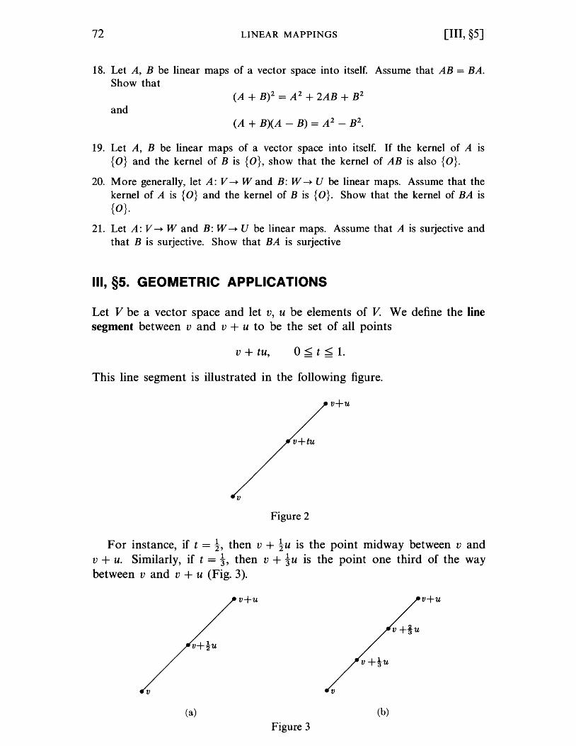
72 LINEAR MAPPINGS [III, §5]
18. Let A, B be linear maps of a vector space into itself. Assume that AB = BA. Show that
(A + B)2 = A 2 + 2AB + B2 and
19. Let A, B be linear maps of a vector space into itself. If the kernel of A is {O} and the kernel of B is {O}, show that the kernel of AB is also {O}.
20. More generally, let A: V --+ Wand B: W --+ U be linear maps. Assume that the kernel of A is {O} and the kernel of B is {O}. Show that the kernel of BA is {O}.
21. Let A: V --+ Wand B: W --+ U be linear maps. Assume that A is surjective and that B is surjective. Show that BA is surjective
III, §5. GEOMETRIC APPLICATIONS
Let V be a vector space and let v, u be elements of V. We define the line segment between v and v + u to be the set of all points
v + tu, o < t < 1.
This line segment is illustrated in the following figure.
v+u
v+tu
v
Figure 2
For instance, if t = t, then v + tU is the point midway between v and v + u. Similarly, if t = t, then v + tu is the point one third of the way between v and v + u (Fig. 3).
v+u v+u
v+!u v+!u
v+tU
v v
(a) (b)
Figure 3
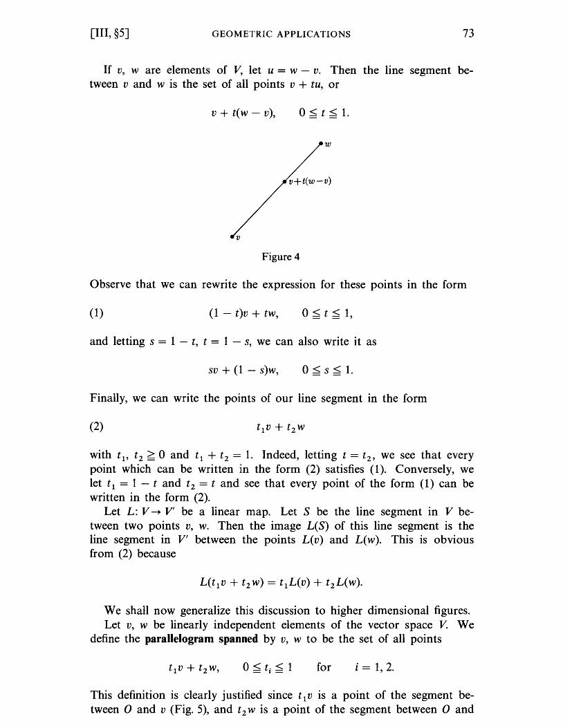
[III, §5] GEOMETRIC APPLICATIONS 73
If v, ware elements of V, let u = w - v. Then the line segment between v and w is the set of all points v + tu, or
v + t(w - v), o < t < 1.
w
v+t(w-v)
v
Figure 4
Observe that we can rewrite the expression for these points in the form
(1) (1 - t)v + tw, o < t < 1,
and letting s = 1 - t, t = 1 - s, we can also write it as
sv + (1 - s)w, o <s< 1.
Finally, we can write the points of our line segment in the form
(2)
with t 1, t2 > 0 and t1 + t2 = 1. Indeed, letting t = t 2, we see that every point which can be written in the form (2) satisfies (1). Conversely, we let t1 = 1 - t and t2 = t and see that every point of the form (1) can be written in the form (2).
Let L: V --+ V' be a linear map. Let S be the line segment in V between two points v, w. Then the image L(S) of this line segment is the line segment in V' between the points L(v) and L(w). This is obvious from (2) because
We shall now generalize this discussion to higher dimensional figures. Let v, w be linearly independent elements of the vector space V. We
define the parallelogram spanned by v, w to be the set of all points
for i = 1, 2.
This definition is clearly justified since t 1 v is a point of the segment between 0 and v (Fig. 5), and t2 w is a point of the segment between 0 and
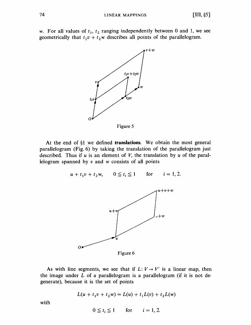
74 LINEAR MAPPINGS [III, §5]
w. For all values of tb t2 ranging independently between 0 and 1, we see geometrically that t 1 V + t 2 W describes all points of the parallelogram.
v+w
Figure 5
At the end of §1 we defined translations. We obtain the most general parallelogram (Fig. 6) by taking the translation of the parallelogram just described. Thus if u is an element of V, the translation by u of the parallelogram spanned by v and w consists of all points
for i = 1, 2.
u+u+w
Figure 6
As with line segments, we see that if L: V --+ V' is a linear map, then the image under L of a parallelogram is a parallelogram (if it is not degenerate), because it is the set of points
with
for i = 1, 2.
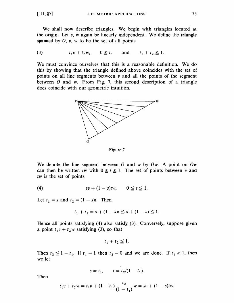
[III, §5] GEOMETRIC APPLICATIONS 75
We shall now describe triangles. We begin with triangles located at the origin. Let v, w again be linearly independent. We define the triangle spanned by 0, v, w to be the set of all points
(3) and
We must convince ourselves that this is a reasonable definition. We do this by showing that the triangle defined above coincides with the set of points on all line segments between v and all the points of the segment between 0 and w. From Fig. 7, this second description of a triangle does coincide with our geometric intuition.
V~~3=~==----------------~W
o
Figure 7
We denote the line segment between 0 and w by Ow. A point on Ow can then be written tw with 0 < t < 1. The set of points between v and tw is the set of points
(4) sv + (1 - s)tw, o <s< 1.
Let t1 = sand t2 = (1 - s)t. Then
t1 + t2 = S + (1 - s)t < s + (1 - s) < 1.
Hence all points satisfying (4) also satisfy (3). Conversely, suppose given a point t1 v + t2 w satisfying (3), so that
Then t2 < 1 - t 1. If t1 = 1 then t2 = 0 and we are done. If t1 < 1, then we let
Then
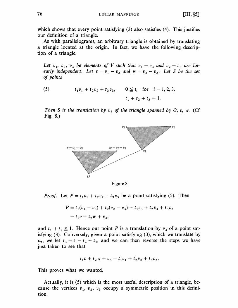
76 LINEAR MAPPINGS [III, §5]
which shows that every point satisfying (3) also satisfies (4). This justifies our definition of a triangle.
As with parallelograms, an arbitrary triangle is obtained by translating a triangle located at the origin. In fact, we have the following description of a triangle.
Let V1, v2, V3 be elements of V such that V1 - V3 and V2 - V3 are linearly independent. Let v = V1 - V3 and w = V2 - v3. Let S be the set of points
(5) o <ti for i = 1, 2, 3,
t1 + t2 + t3 = 1.
Then S is the translation by V3 of the triangle spanned by 0, v, w. (Cf. Fig. 8.)
Figure 8
Proof. Let P = t1v1 + t2v2 + t3v3 be a point satisfying (5). Then
and t1 + t2 < 1. Hence our point P is a translation by V3 of a point satisfying (3). Conversely, given a point satisfying (3), which we translate by V3, we let t3 = 1 - t2 - t 1, and we can then reverse the steps we have just taken to see that
This proves what we wanted.
Actually, it is (5) which is the most useful description of a triangle, because the vertices V1, V2, V3 occupy a symmetric position in this definition.
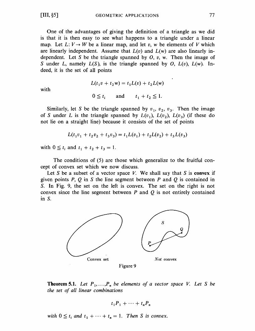
[III, §5] GEOMETRIC APPLICATIONS 77
One of the advantages of giving the definition of a triangle as we did is that it is then easy to see what happens to a triangle under a linear map. Let L: V --+ W be a linear map, and let v, w be elements of V which are linearly independent. Assume that L( v) and L( w) are also linearly independent. Let S be the triangle spanned by 0, v, w. Then the image of Sunder L, namely L(S), is the triangle spanned by 0, L(v), L(w). Indeed, it is the set of all points
with and
Similarly, let S be the triangle spanned by v 1, v2 , v3. Then the image of Sunder L is the triangle spanned by L(v 1), L(v2 ), L(V3) (if these do not lie on a straight line) because it consists of the set of points
The conditions of (5) are those which generalize to the fruitful concept of convex set which we now discuss.
Let S be a subset of a vector space V. We shall say that S is convex if given points P, Q in S the line segment between P and Q is contained in S. In Fig. 9, the set on the left is convex. The set on the right is not convex since the line segment between P and Q is not entirely contained in S.
Convex set Not convex
Figure 9
Theorem 5.1. Let P l' ... ,P n be elements of a vector space V. Let S be the set of all linear combinations
with 0 < ti and t1 + ... + tn = 1. Then S is convex.
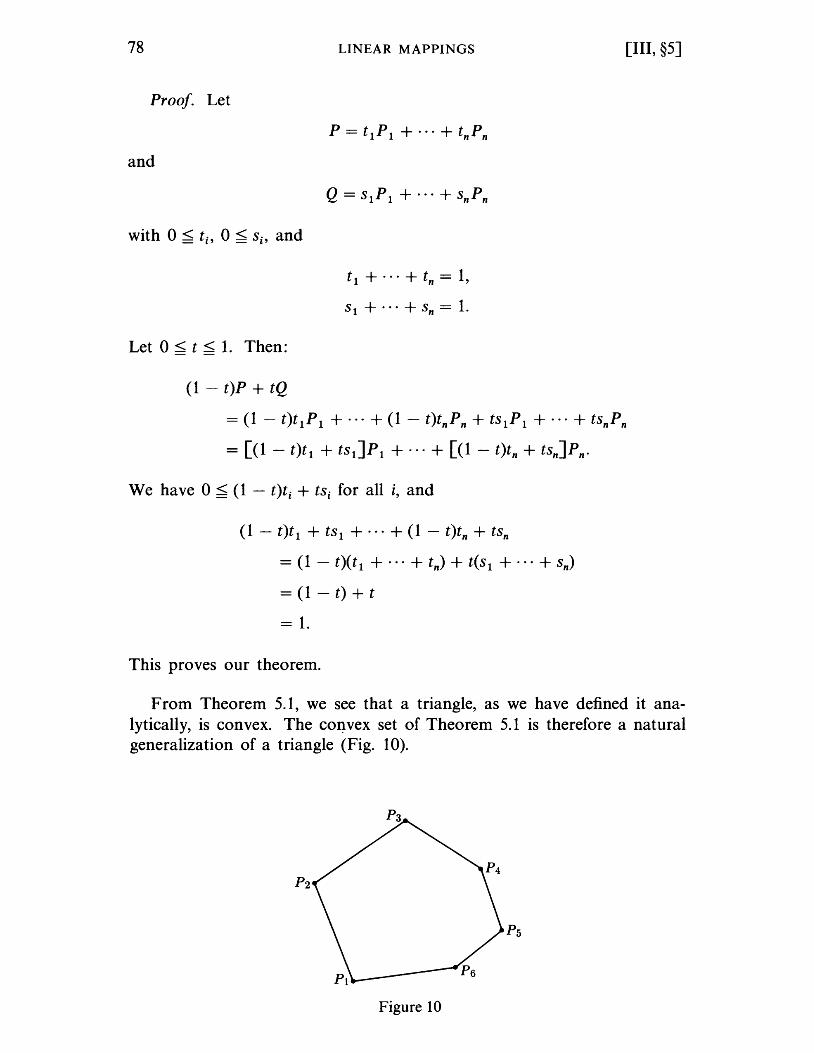
78 LINEAR MAPPINGS [III, §5]
Proof. Let
and
Q =SP +···+SP 1 1 n n
t +···+t =1 1 n'
S1 + ... + Sn = 1.
Let 0 < t < 1. Then:
(1 - t)P + tQ
= (1 - t)t 1P 1 + ... + (1 - t)tnPn + ts 1P 1 + ... + tSnPn
= [(1 - t)t1 + ts1]p 1 + ... + [(1 - t)tn + tsn]Pn·
We have 0 < (1 - t)ti + tSi for all i, and
(1 - t)t 1 + ts 1 + ... + (1 - t)tn + tSn
= (1 - t)( t 1 + ... + tn) + t( S 1 + . .. + Sn)
= (1 - t) + t = 1.
This proves our theorem.
From Theorem 5.1, we see that a triangle, as we have defined it analytically, is convex. The co~vex set of Theorem 5.1 is therefore a natural generalization of a triangle (Fig. 10).
Ps
Figure 10
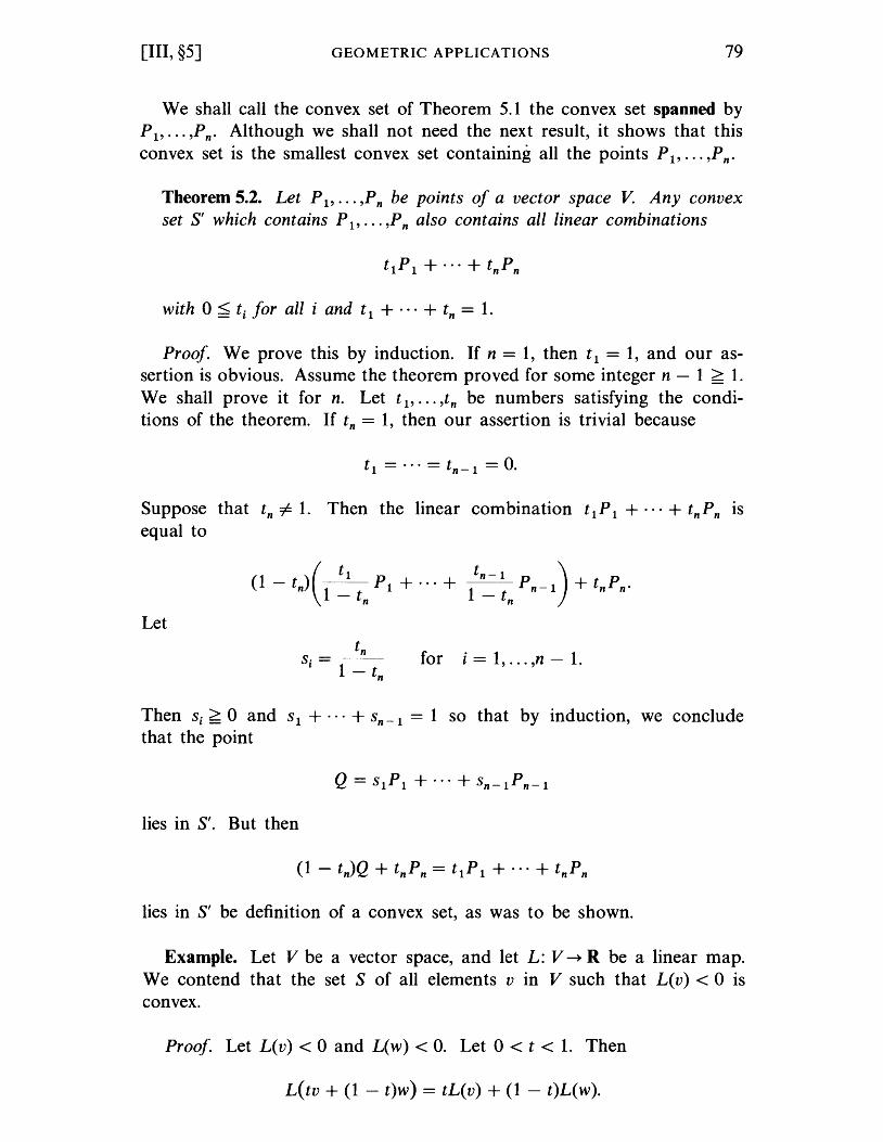
[III, §5] GEOMETRIC APPLICATIONS 79
We shall call the convex set of Theorem 5.1 the convex set spanned by P 1"" ,Pn • Although we shall not need the next result, it shows that this convex set is the smallest convex set containing all the points P 1'··· ,Pn •
Theorem 5.2. Let P l' ... ,P n be points of a vector space V. Any convex set S' which contains P l' ... ,P n also contains all linear combinations
with 0 < ti for all i and t1 + ... + tn = 1.
Proof. We prove this by induction. If n = 1, then t1 = 1, and our assertion is obvious. Assume the theorem proved for some integer n - 1 > 1. We shall prove it for n. Let t l' ... ,tn be numbers satisfying the conditions of the theorem. If tn = 1, then our assertion is trivial because
t1 = ... = tn- 1 = o.
Suppose that tn i= 1. Then the linear combination t 1P 1 + ... + tnPn IS
equal to
Let tn
s·=--l 1 - t
n
for i = 1, ... ,n - 1.
Then Si > 0 and S1 + ... + Sn-1 = 1 so that by induction, we conclude that the point
lies in S'. But then
lies in S' be definition of a convex set, as was to be shown.
Example. Let V be a vector space, and let L: V ~ R be a linear map. We contend that the set S of all elements v in V such that L(v) < 0 is convex.
Proof. Let L(v) < 0 and L(w) < O. Let 0 < t < 1. Then
L{tv + (1 - t)w) = tL(v) + (1 - t)L(w).
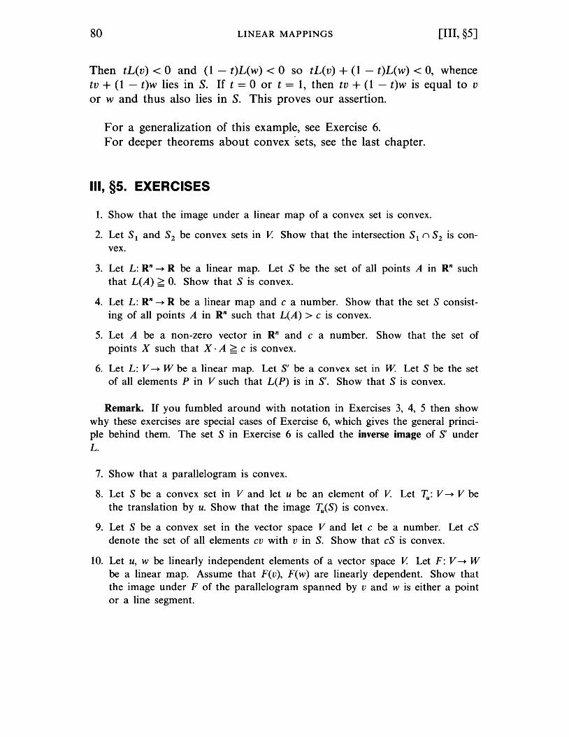
80 LINEAR MAPPINGS [III, §5]
Then tL(v) < 0 and (1 - t)L(w) < 0 so tL(v) + (1 - t)L(w) < 0, whence tv + (1 - t)w lies in S. If t = 0 or t = 1, then tv + (1 - t)w is equal to v or wand thus also lies in S. This proves our assertion.
F or a generalization of this example, see Exercise 6. For deeper theorems about convex ·sets, see the last chapter.
III, §5. EXERCISES
1. Show that the image under a linear map of a convex set is convex.
2. Let S 1 and S2 be convex sets in V. Show that the intersection S 1 (\ S2 is convex.
3. Let L: Rn ~ R be a linear map. Let S be the set of all points A in Rn such that L(A) ~ O. Show that S is convex.
4. Let L: Rn ~ R be a linear map and c a number. Show that the set S consisting of all points A in Rn such that L(A) > c is convex.
5. Let A be a non-zero vector in Rn and c a number. Show that the set of points X such that X· A ~ c is convex.
6. Let L: V ~ W be a linear map. Let Sf be a convex set in W Let S be the set of all elements P in V such that L(P) is in Sf. Show that S is convex.
Remark. If you fumbled around with notation in Exercises 3, 4, 5 then show why these exercises are special cases of Exercise 6, which gives the general principle behind them. The set S in Exercise 6 is called the inverse image of Sf under L.
7. Show that a parallelogram is convex.
8. Let S be a convex set in V and let u be an element of V. Let ~: V ~ V be the translation by u. Show that the image ~(S) is convex.
9. Let S be a convex set in the vector space V and let c be a number. Let cS denote the set of all elements cv with v in S. Show that cS is convex.
10. Let u, w be linearly independent elements of a vector space V. Let F: V ~ W be a linear map. Assume that F(v), F(w) are linearly dependent. Show that the image under F of the parallelogram spanned by v and w is either a point or a line segment.
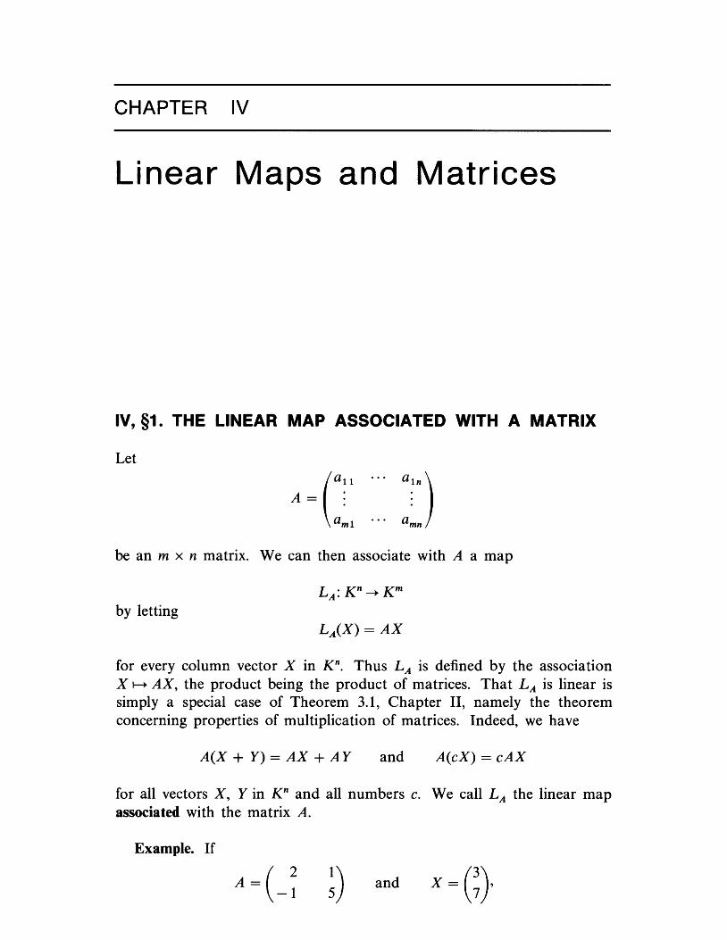
CHAPTER IV
Linear Maps and Matrices
IV, §1. THE LINEAR MAP ASSOCIATED WITH A MATRIX
Let
be an m x n matrix. We can then associate with A a map
by letting
for every column vector X in Kn. Thus LA is defined by the association X t--+ AX, the product being the product of matrices. That LA is linear is simply a special case of Theorem 3.1, Chapter II, namely the theorem concerning properties of multiplication of matrices. Indeed, we have
A(X + Y) = AX + A Y and A(cX) = cAX
for all vectors X, Y in K n and all numbers c. We call LA the linear map associated with the matrix A.
Example. If
A = ( 2 -1 !) and x=G}
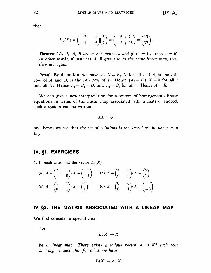
82 LINEAR MAPS AND MATRICES [IV, §2]
then
Theorem 1.1. If A, Bare m x n matrices and if LA = L B , then A = B. I n other words, if matrices A, B give rise to the same linear map, then they are equal.
Proof By definition, we have Ai· X = B i · X for all i, if Ai is the i-th row of A and Bi is the i-th row of B. Hence (Ai - Bi)· X = 0 for all i and all X. Hence Ai - Bi = 0, and Ai = Bi for all i. Hence A = B.
We can give a new interpretation for a system of homogeneous linear equations in terms of the linear map associated with a matrix. Indeed, such a system can be written
AX = 0,
and hence we see that the set of solutions is the kernel of the linear map
LA·
IV, §1. EXERCISES
1. In each case, find the vector LA(X).
(a) A = G (c) A = G
~}x=(_~)
~}x=G)
(b) A = G (d) A = (~
~}x=G)
~}x = (_~)
IV, §2. THE MATRIX ASSOCIATED WITH A LINEAR MAP
We first consider a special case.
Let
be a linear map. There exists a unique vector A in K n such that L = LA' i.e. such that for all X we have
L(X) = A·X.
[IV, §2] THE MATRIX ASSOCIATED WITH A LINEAR MAP 83
Let E1, ... ,En be the unit vectors in Kn. If X = x 1E1 + ... + xnEn is any vector, then
L(X) = L(X1E1 + ... + xnEn)
= x 1L(E1) + ... + xnL(En)·
If we now let
we see that
This proves what we wanted. It also gives us an explicit determination of the vector A such that L = LA' namely the components of A are precisely the values L(E 1), ... ,L(En), where Ei (i = 1, ... ,n) are the unit vectors of Kn.
We shall now generalize this to the case of an arbitrary linear map into K m
, not just into K.
Theorem 2.1. Let L: K n ---+ K m be a linear map. Then there exists a
unique matrix A such that L = LA.
Proof As usual, let E1, ... ,En be the unit column vectors in K n, and let e1, ... ,em be the unit column vectors in Km. We can write any vector X in K n as a linear combination
where Xj is the j-th component of X. We view E1, ... ,En as column vectors. By linearity, we find that
and we can write each L(Ej) in terms of e1, ... ,em. In other words, there exist numbers aij such that
84 LINEAR MAPS AND MATRICES [IV, §2]
or in terms of the column vectors,
Hence
L(X) = xl(alle l + ... + amlem) + ... + xn(alne l + ... + amnem)
= (allx l + ... + alnxn)e l + ... + (amlx l + ... + amnxn)em.
Consequently, if we let A = (aij), then we see that
L(X) = AX.
Written out in full, this reads
Thus L = LA is the linear map associated with the matrix A. We also call A the matrix associated with the linear map L. We know that this matrix is uniquely determined by Theorem 1.1.
Example 1. Let F: R3 ---+ R2 be the projection, in other words the mapping such that F(Xl' X2 , x 3) = (Xl' X 2 ). Then the matrix associated with F is
(1 0 0). 010
Example 2. Let I: Rn ---+ Rn be the identity. Then the matrix associated with I is the matrix
100 0
010 0
000 1
having components equal to 1 on the diagonal, and 0 otherwise.
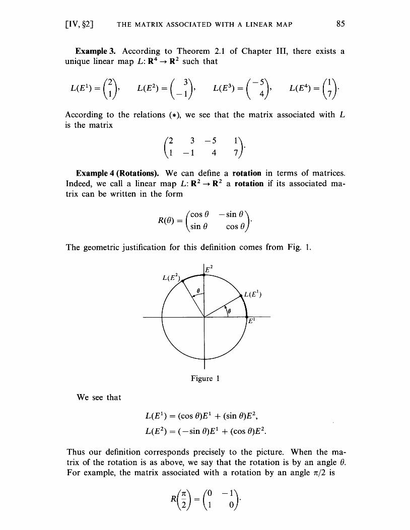
[IV, §2] THE MATRIX ASSOCIATED WITH A LINEAR MAP 85
Example 3. According to Theorem 2.1 of Chapter III, there exists a unique linear map L: R4 ---+ R2 such that
According to the relations (*), we see that the matrix associated with L is the matrix
3
-1 -5
4
Example 4 (Rotations). We can define a rotation in terms of matrices. Indeed, we call a linear map L: R2 ---+ R2 a rotation if its associated matrix can be written in the form
R( ) = . e (COS e SIn e
-sin e). cos e
The geometric justification for this definition comes from Fig. 1.
We see that
Figure 1
L(E1) = (cos e)E1 + (sin e)E2,
L(E2) = (-sin e)E1 + (cos e)E2.
Thus our definition corresponds precisely to the picture. When the matrix of the rotation is as above, we say that the rotation is by an angle e. For example, the matrix associated with a rotation by an angle n/2 is
86 LINEAR MAPS AND MATRICES [IV, §2]
We observe finally that the operations on matrices correspond to the operations on the associated linear map. For instance, if A, Bare m x n matrices, then
and if c is a number, then
This is obvious, because
(A + B)X = AX + BX and (cA)X = c(AX).
Similarly for compositions of mappings. Indeed, let
and
be linear maps, and let A, B be the matrices associated with F and G respectively. Then for any vector X in K n we have
(G 0 F)(X) = G(F(X)) = B(AX) = (BA)X.
Hence the product BA is the matrix associated with the composite linear map GoF.
Theorem 2.2. Let A be an n x n matrix, and let A 1, ... ,An be its columns. Then A is invertible if and only if A 1, ... ,An are linearly independent.
Proof. Suppose A 1, ... ,An are linearly independent. Then {A 1, ... ,An} is a basis of K n, so the unit vectors E 1
, ... ,En can be expressed as linear combinations of A 1, ... ,An. This means that there is a matrix B such that
for j = 1, ... ,n,
say by Theorem 2.1 of Chapter III. But this is equivalent to saying that BA = I. Thus A is invertible. Conversely, suppose A is invertible. The linear map LA is such that
Since A is invertible, we must have Ker LA = 0, because if AX = 0 then A -1 AX = X = O. Hence A 1, ... ,An are linearly independent. This proves the theorem.
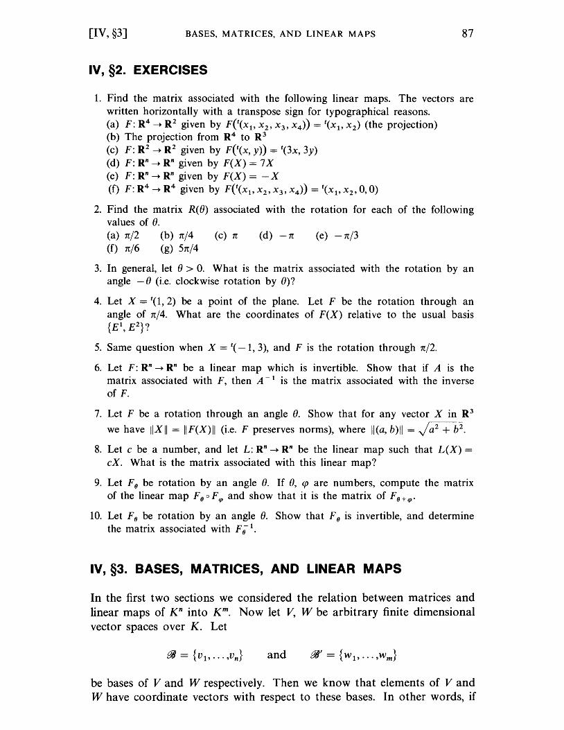
[IV, §3] BASES, MATRICES, AND LINEAR MAPS 87
IV, §2. EXERCISES
1. Find the matrix associated with the following linear maps. The vectors are written horizontally with a transpose sign for typographical reasons. (a) F: R4 --+ R2 given by F(t(Xl' X2 , X3 , x 4 )) = t(Xl' x 2 ) (the projection) (b) The projection from R4 to R3 (c) F: R2 --+ R2 given by F(t(x, y)) = t(3x, 3y) (d) F: Rn
--+ Rn given by F(X) = 7 X (e) F: Rn
--+ Rn given by F(X) = -X (f) F: R4 --+ R4 given by F('(x t , X2 , X3 , x 4 )) = t(Xl' X2 , 0, 0)
2. Find the matrix R(e) associated with the rotation for each of the following values of e. (a) n/2 (b) n/4 (c) n (d) -n (e) -n/3 (f) n/6 (g) 5n/4
3. In general, let e > O. What is the matrix associated with the rotation by an angle - e (i.e. clockwise rotation bye)?
4. Let X = t(l, 2) be a point of the plane. Let F be the rotation through an angle of n/4. What are the coordinates of F(X) relative to the usual basis {Et,E2}?
5. Same question when X = t( -1, 3), and F is the rotation through n/2.
6. Let F: Rn --+ Rn be a linear map which is invertible. Show that if A is the matrix associated with F, then A - 1 is the matrix associated with the inverse of F.
7. Let F be a rotation through an angle e. Show that for any vector X in R 3
we have ,IXII = IIF(X)II (i.e. F preserves norms), where II(a, b)11 = J a2 + b2•
8. Let e be a number, and let L: Rn --+ Rn be the linear map such that L(X) =
eX. What is the matrix associated with this linear map?
9. Let Fo be rotation by an angle e. If e, <p are numbers, compute the matrix of the linear map Fo 0 F cp and show that it is the matrix of Fo+cp.
10. Let Fo be rotation by an angle e. Show that F 0 is invertible, and determine the matrix associated with F (; 1.
IV, §3. BASES, MATRICES, AND LINEAR MAPS
In the first two sections we considered the relation between matrices and linear maps of Kn into Km. Now let V, W be arbitrary finite dimensional vector spaces over K. Let
and
be bases of V and W respectively. Then we know that elements of V and W have coordinate vectors with respect to these bases. In other words, if
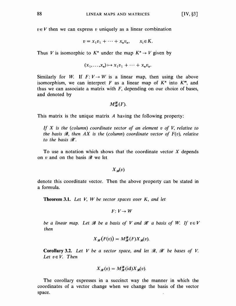
88 LINEAR MAPS AND MATRICES [IV, §3]
V E V then we can express v uniquely as a linear combination
Thus V is isomorphic to Kn under the map Kn ---+ V given by
Similarly for W. If F: V ---+ W is a linear map, then using the above isomorphism, we can interpret F as a linear map of Kn into Km, and thus we can associate a matrix with F, depending on our choice of bases, and denoted by
This matrix is the unique matrix A having the following property:
If X is the (column) coordinate vector of an element v of V, relative to the basis 81, then AX is the (column) coordinate vector of F(v), relative to the basis 81'.
To use a notation which shows that the coordinate vector X depends on v and on the basis 81 we let
X 8iJ(v)
denote this coordinate vector. Then the above property can be stated in a formula.
Theorem 3.1. Let V, W be vector spaces over K, and let
F: V---+ W
be a linear map. Let 81 be a basis of V and 81' a basis of W If v E V then
Corollary 3.2. Let V be a vector space, and let 81, 81' be bases of V. Let v E V. Then
The corollary expresses in a succinct way the manner in which the coordinates of a vector change when we change the basis of the vector space.
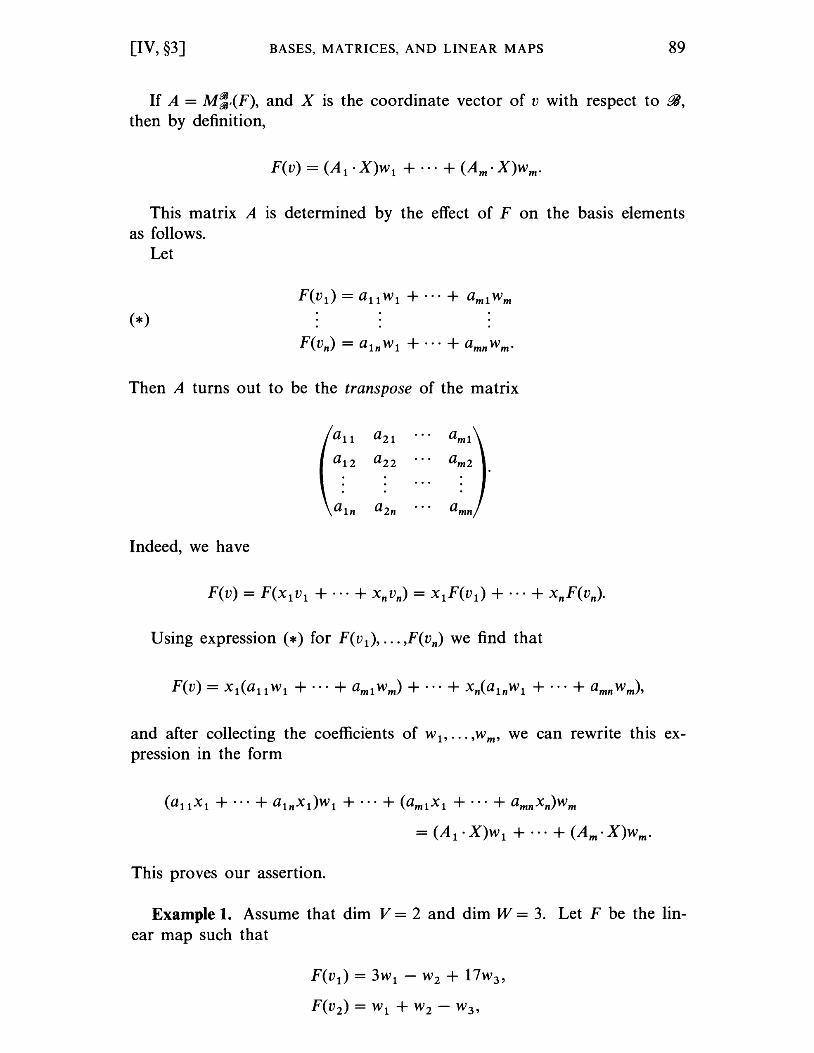
[IV, §3] BASES, MATRICES, AND LINEAR MAPS 89
If A = M:,(F), and X is the coordinate vector of v with respect to 84, then by definition,
This matrix A is determined by the effect of F on the basis elements as follows.
Let
Then A turns out to be the transpose of the matrix
all a2l aml
a12 a22 am2
Indeed, we have
Using expression (*) for F(v l ), ..• ,F(vn) we find that
and after collecting the coefficients of W l , ... ,Wm , we can rewrite this expression in the form
This proves our assertion.
Example 1. Assume that dim V = 2 and dim W = 3. Let F be the linear map such that
F(v l ) = 3w l - W2 + 17w3 ,
F(v 2 ) = W l + W 2 - W 3 ,
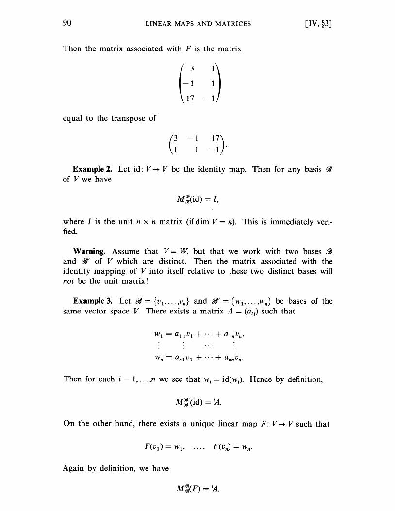
90 LINEAR MAPS AND MATRICES
Then the matrix associated with F is the matrix
equal to the transpose of
( 3 1)
-1 1
17 -1
-1 1
[IV, §3]
Example 2. Let id: V ~ V be the identity map. Then for any basis fIJ of V we have
where I is the unit n x n matrix (if dim V = n). This is immediately verified.
Warning. Assume that V = W, but that we work with two bases fIJ and fIJ' of V which are distinct. Then the matrix associated with the identity mapping of V into itself relative to these two distinct bases will not be the unit matrix!
Example 3. Let fIJ = {v 1, ... ,vn} and fIJ' = {W1' ... ,wn} be bases of the same vector space V. There exists a matrix A = (aij) such that
Then for each i = 1, ... ,n we see that Wi = id(wi). Hence by definition,
On the other hand, there exists a unique linear map F: V ~ V such that
F(v 1 ) = w 1, ••• , F(vn) = wn •
Again by definition, we have
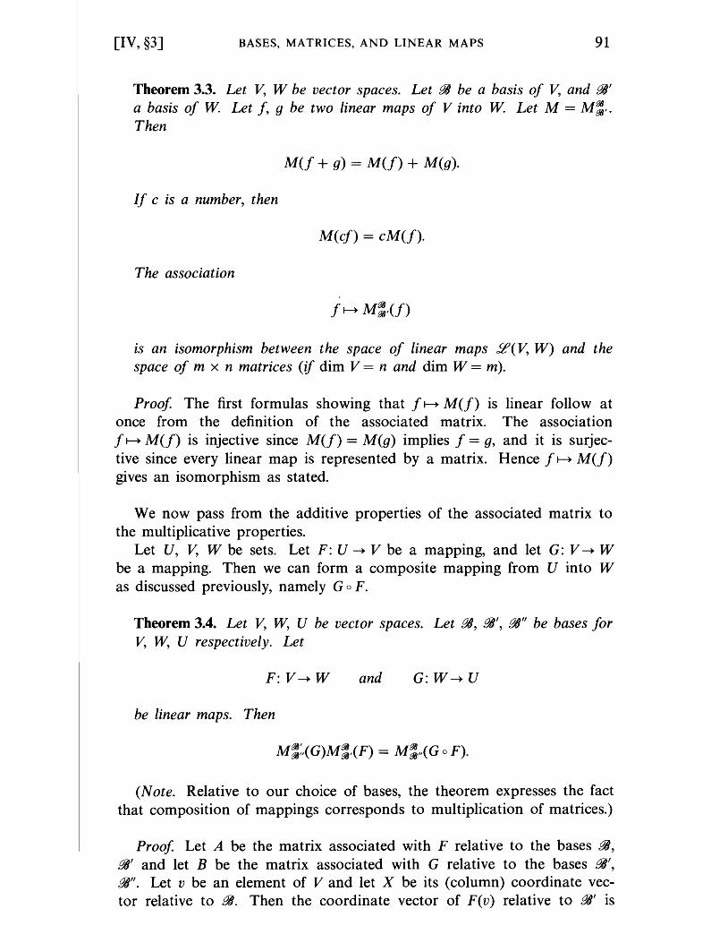
[IV, §3] BASES, MATRICES, AND LINEAR MAPS 91
Theorem 3.3. Let V, W be vector spaces. Let PA be a basis of V, and PA' a basis of W. Let f, g be two linear maps of V into W. Let M = M:,. Then
M(f + g) = M(f) + M(g).
If c is a number, then
M(cf) = cM(f)·
The association
is an isomorphism between the space of linear maps 5l'(V, W) and the space of m x n matrices (if dim V = n and dim W = m).
Proof. The first formulas showing that fl-+ M(f) is linear follow at once from the definition of the associated matrix. The association fl-+ M(f) is injective since M(f) = M(g) implies f = g, and it is surjective since every linear map is represented by a matrix. Hence fl-+ M(f) gives an isomorphism as stated.
We now pass from the additive properties of the associated matrix to the multiplicative properties.
Let U, V, W be sets. Let F: U --.. V be a mapping, and let G: V --.. W be a mapping. Then we can form a composite mapping from U into W as discussed previously, namely Go F.
Theorem 3.4. Let V, W, U be vector spaces. Let PA, PA', PA" be bases for V, W, U respectively. Let
F: V--.. W and G: W--.. U
be linear maps. Then
(Note. Relative to our choice of bases, the theorem expresses the fact that composition of mappings corresponds to multiplication of matrices.)
Proof. Let A be the matrix associated with F relative to the bases PA, PA' and let B be the matrix associated with G relative to the bases PA', PA". Let v be an element of V and let X be its (column) coordinate vector relative to PA. Then the coordinate vector of F(v) relative to PA' is
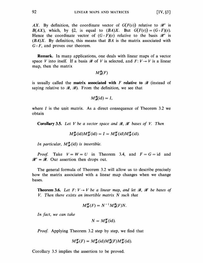
92 LINEAR MAPS AND MATRICES [IV, §3]
AX. By definition, the coordinate vector of G(F(v)) relative to PA" is B(AX), which, by §2, is equal to (BA)X. But G(F(v)) = (G 0 F)(v). Hence the coordinate vector of (G 0 F)( v) relative to the basis PA" is (BA)X. By definition, this means that BA is the matrix associated with G 0 F, and proves our theorem.
Remark. In many applications, one deals with linear maps of a vector space V into itself. If a basis PA of V is selected, and F: V --.. V is a linear map, then the matrix
is usually called the matrix associated with F relative to PA (instead of saying relative to PA, PA). From the definition, we see that
where I is the unit matrix. As a direct consequence of Theorem 3.2 we obtain
Corollary 3.5. Let V be a vector space and PA, PA' bases of V. Then
In particular, M:,(id) is invertible.
Proof. Take V = W = U in Theorem 3.4, and F = G = id and 14" = 14. Our assertion then drops out.
The general formula of Theorem 3.2 will allow us to describe precisely how the matrix associated with a linear map changes when we change bases.
Theorem 3.6. Let F: V --.. V be a linear map, and let PA, PA' be bases of V. Then there exists an invertible matrix N such that
I n fact, we can take
Proof. Applying Theorem 3.2 step by step, we find that
Corollary 3.5 implies the assertion to be proved.
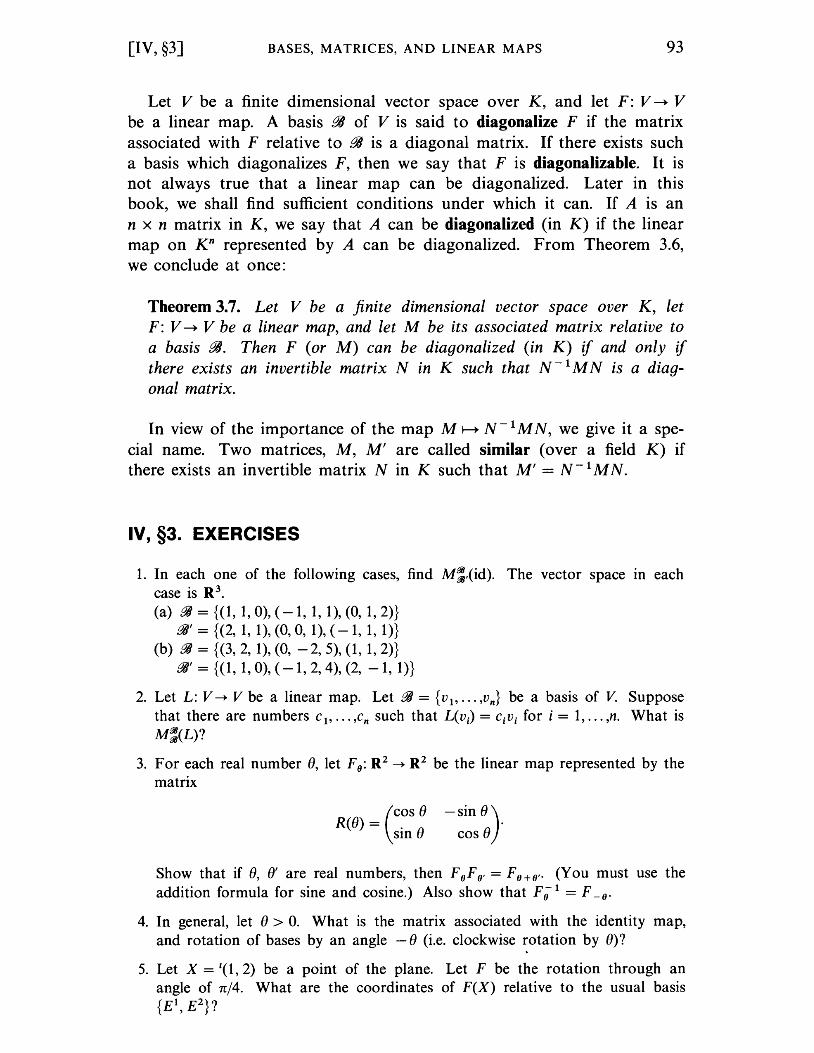
[IV, §3] BASES, MATRICES, AND LINEAR MAPS 93
Let V be a finite dimensional vector space over K, and let F: V --+ V be a linear map. A basis f!4 of V is said to diagonalize F if the matrix associated with F relative to f!4 is a diagonal matrix. If there exists such a basis which diagonalizes F, then we say that F is diagonalizable. It is not always true that a linear map can be diagonalized. Later in this book, we shall find sufficient conditions under which it can. If A is an n x n matrix in K, we say that A can be diagonalized (in K) if the linear map on Kn represented by A can be diagonalized. From Theorem 3.6, we conclude at once:
Theorem 3.7. Let V be a finite dimensional vector space over K, let F: V --+ V be a linear map, and let M be its associated matrix relative to a basis f!4. Then F (or M) can be diagonalized (in K) if and only if there exists an invertible matrix N in K such that N - 1 M N is a diagonal matrix.
In view of the importance of the map M r--. N- 1 MN, we give it a special name. Two matrices, M, M' are called similar (over a field K) if there exists an invertible matrix N in K such that M' = N - 1 M N.
IV, §3. EXERCISES
1. In each one of the following cases, find M:,(id). The vector space in each case is R3. (a) (JI = {(I, 1,0), (-1, 1, 1), (0, 1, 2)}
(JI' = {(2, 1, 1), (0, 0, 1), ( -1, 1, I)} (b) (JI = {(3, 2,1), (0, -2,5), (1,1, 2)}
(JI' = {(I, 1,0), (-1,2,4), (2, -1, I)}
2. Let L: V ~ V be a linear map. Let (JI = {Vi'.'. ,Vn} be a basis of V. Suppose that there are numbers C i , ... 'Cn such that L(vi) = CiVi for i = 1, ... ,no What is M:(L)?
3. For each real number f), let Fo: R2 ~ R2 be the linear map represented by the matrix
R(8) = . (
COS f) - sin f) ) sin f) cos f)
Show that if f), f)' are real numbers, then FoFo' = Fo+o" (You must use the addition formula for sine and cosine.) Also show that FiJi = F -0'
4. In general, let f) > 0. What is the matrix associated with the identity map, and rotation of bases by an angle - f) (i.e. clockwise rotation by 8)?
5. Let X = t(l, 2) be a point of the plane. Let F be the rotation through an angle of n/4. What are the coordinates of F(X) relative to the usual basis {El,E2}?
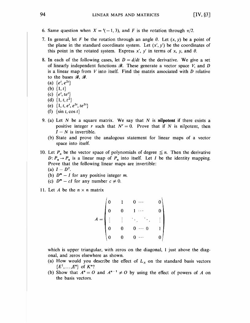
94 LINEAR MAPS AND MATRICES [IV, §3]
6. Same question when X = t( - 1, 3), and F is the rotation through n/2.
7. In general, let F be the rotation through an angle O. Let (x, y) be a point of the plane in the standard coordinate system. Let (x', y') be the coordinates of this point in the rotated system. Express x', y' in terms of x, y, and O.
8. In each of the following cases, let D = d/dt be the derivative. We give a set of linearly independent functions fJl. These generate a vector space V, and D is a linear map from V into itself. Find the matrix associated with D relative to the bases fJl, fJl. (a) {e t
, e2t}
(b) {I, t} (c) {e t, tet} (d) {1,t,t2} (e) {1, t, et
, e2t, te2t
}
(f) {sin t, cos t}
9. (a) Let N be a square matrix. We say that N is nilpotent if there exists a positive integer r such that N r = O. Prove that if N is nilpotent, then I - N is invertible.
(b) State and prove the analogous statement for linear maps of a vector space into itself.
10. Let Pn be the vector space of polynomials of degree ~ n. Then the derivative D: Pn ~ Pn is a linear map of Pn into itself. Let I be the identity mapping. Prove that the following linear maps are invertible: (a) I - D2. (b) Dm
- I for any positive integer m. (c) Dm
- cI for any number c i= O.
11. Let A be the n x n matrix
A=
o
o
o
o
1
o
o
o
o 1
o
o o
o
o
1
o
which is upper triangular, with zeros on the diagonal, 1 just above the diagonal, and zeros elsewhere as shown. (a) How would you describe the effect of LA on the standard basis vectors
{E1, ... ,En} of K n? (b) Show that An = 0 and An - 1 i= 0 by using the effect of powers of A on
the basis vectors.
CHAPTER V
Scalar Products and Orthogonal ity
V, §1. SCALAR PRODUCTS
Let V be a vector space over a field K. A scalar product on V is an association which to any pair of elements v, W of V associates a scalar, denoted by (v, w), or also V· w, satisfying the following properties:
SP 1. We have (v, w) = (w, v) for all v, WE V.
SP 2. If u, v, ware elements of V, then
(u, v + w) = (u, v) + (u, w).
SP 3. If xEK, then
(xu, v) = x(u, v) and (u, xv) = x(u, v).
The scalar product is said to be non-degenerate if in addition it also satisfies the condition:
If v is an element of V, and (v, w) = 0 for all WE V, then v = O.
Example 1. Let V = Kn. Then the map
(X, Y) r-+ X . Y,
which to elements X, Y E K n associates their dot product as we defined it previously, is a scalar product in the present sense.
96 SCALAR PRODUCTS AND ORTHOGONALITY [V, §1]
Example 2. Let V be the space of continuous real-valued functions on the interval [0, 1]. If j, g E V, we define
<I, g) = L1/(t)g(t) dt.
Simple properties of the integral show that this is a scalar product.
In both examples the scalar product is non-degenerate. We had pointed this out previously for the dot product of vectors in Kn. In the second example, it is also easily shown from simple properties of the integral.
In calculus, we study the second example, which gives rise to the theory of Fourier series. Here we discuss only general properties of scalar products and applications to Euclidean spaces. The notation < , > is used because in dealing with vector spaces of functions, a dot j. g may be confused with the ordinary product of functions.
Let V be a vector space with a scalar product. As always, we define elements v, w of V to be orthogonal or perpendicular, and write v ~ w, if < v, w> = O. If S is a subset of V, we denote by S.l the set of all elements WE V which are perpendicular to all elements of S, i.e. < w, v> = 0 for all v E S. Then using SP 2 and SP 3, one verifies at once that S.l is a subspace of V, called the orthogonal space of S. If W is perpendicular to S, we also write W ~ S. Let U be the subspace of V generated by the elements of S. If W is perpendicular to S, and if v1, V 2 E S, then
If c is a scalar, then
Hence w is perpendicular to linear combinations of elements of S, and hence w is perpendicular to U.
Example 3. Let (aij) be an m x n matrix in K, and let A 1, ••. ,Am be its row vectors. Let X = t(X 1, ... ,Xn) as usual. The system of homogeneous linear equations
can also be written in an abbreviated form, namely
[V, §1] SCALAR PRODUCTS 97
The set of solutions X of this homogeneous system is a vector space over K. In fact, let W be the space generated by A 1, ••• ,Am. Let U be the space consisting of all vectors in K n perpendicular to A l' ... ,Am. Then U is precisely the vector space of solutions of (**). The vectors A 1, ••• ,Am may not be linearly independent. We note that dim W < m, and we call
dim U = dim W-L
the dimension of the space of solutions of the system of linear equations. We shall discuss this dimension at greater length later.
Let V again be a vector space over the field K, with a scalar product. Let {v 1, ••• ,vn } be a basis of V. We shall say that it is an orthogonal
basis if (Vi' V j ) = 0 for all i i= j. We shall show later that if V is a finite dimensional vector space, with a scalar product, then there always exists an orthogonal basis. However, we shall first discuss important special cases over the real and complex numbers.
The real positive definite case
Let V be a vector space over R, with a scalar product. We shall call this scalar product positive definite if (v, v) > 0 for all V E V, and (v, v) > 0 if V i= O. The ordinary dot product of vectors in Rn is positive definite, and so is the scalar product of Example 2 above.
Let V be a vector space over R, with a positive definite scalar product denoted by ( , ). Let W be a subspace. Then W has a scalar product defined by the same rule defining the scalar product in V. In other words, if w, w' are elements of W, we may form their product (w, w'). This scalar product on W is obviously positive definite.
For instance, if W is the subspace of R3 generated by the two vectors (1, 2, 2) and (n, -1, 0), then W is a vector space in its own right, and we can take the dot product of vectors lying in W to define a positive definite scalar product on W We often have to deal with such subspaces, and this is one reason why we develop our theory on arbitrary (finite dimensional) spaces over R with a given positive definite scalar product, instead of working only on Rn with the dot product. Another reason is that we wish our theory to apply to situations as described in Example 2 of §1.
We define the norm of an element v E V by
Ilvll = J (v, v).
If e is any number, then we immediately get
Ilevll = lelllvll,
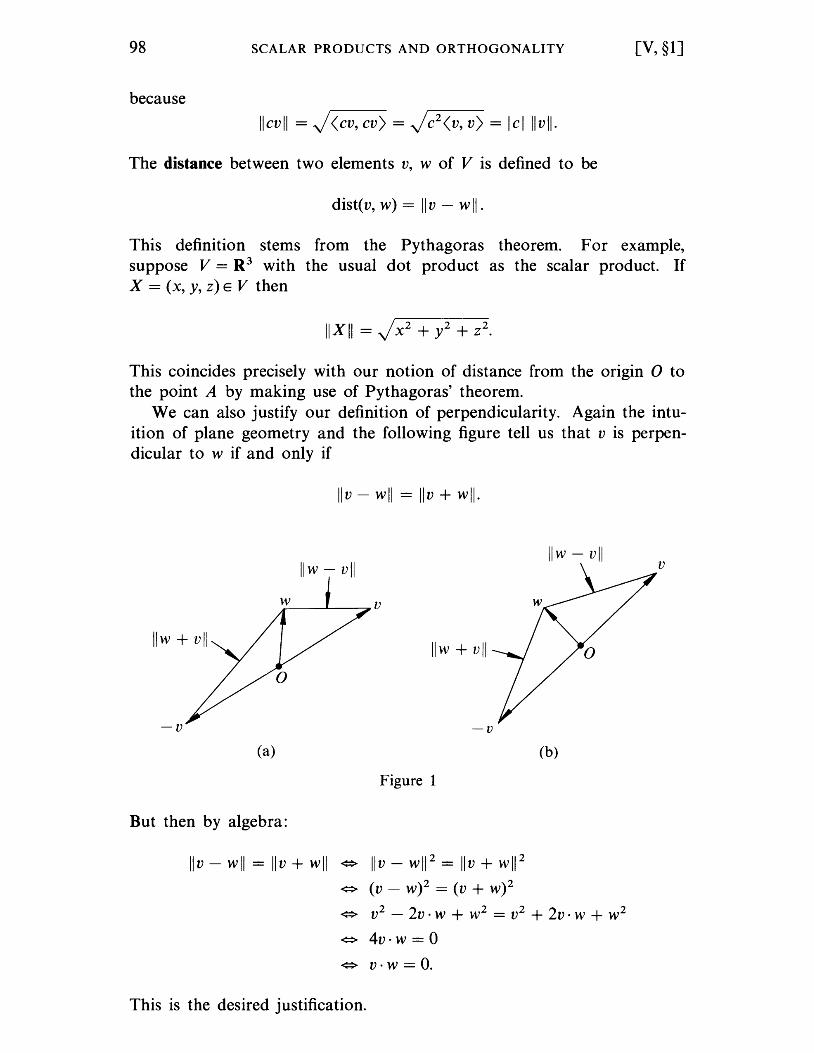
98 SCALAR PRODUCTS AND ORTHOGONALITY [V, §1]
because
Ilevll = J <ev, ev) = Je2 <v, v) = lelllvll·
The distance between two elements v, w of V is defined to be
dist(v, w) = Ilv - wll.
This definition stems from the Pythagoras theorem. For example, suppose V = R3 with the usual dot product as the scalar product. If X = (x, y, z) E V then
This coincides precisely with our notion of distance from the origin 0 to the point A by making use of Pythagoras' theorem.
We can also justify our definition of perpendicularity. Again the intuition of plane geometry and the following figure tell us that v is perpendicular to w if and only if
Ilv - wll = Ilv + wll·
Ilw - vii
__ ....&...-_~v
Ilw + vii IIw + vII o
-v -v
(a)
Figure 1
But then by algebra:
Ilv - wll = Ilv + wll ¢> Ilv - wl12 = Ilv + wl1 2
¢> (v - W)2 = (v + W)2
Ilw - vii
(b)
¢> v2 - 2v . w + w2 = v2 + 2v· w + w2
¢> 4v·w = 0
¢> V·W = O.
This is the desired justification.
v
[V, §1] SCALAR PRODUCTS 99
You probably have studied the dot product of n-tuples in a previous course. Basic properties which were proved without coordinates can be proved for our more general scalar product. We shall carry such proofs out, and meet other examples as we go along.
We say that an element v E V is a unit vector if II v II = 1. If v E V and v -# 0, then viii v II is a unit vector.
The following two identities follow directly from the definition of the length.
The Pythagoras theorem. If v, ware perpendicular, then
The parallelogram law. For any v, w we have
The proofs are tri vial. We give the first, and leave the second as an exercise. For the first, we have
Ilv + wl12 = <v + w,v + w) = <v, v) + 2<v, w) + <w, w)
= IIvl12 + IIwll 2 because v -1 w.
This proves Pythagoras.
Let w be an elelnent of V such that Ilwll -# O. For any v there exists a unique number c such that v - cw is perpendicular to w. Indeed, for v - cw to be perpendicular to w we must have
<v - cw, w) = 0,
whence <v, w) - <cw, w) = 0 and <v, w) = c<w, w). Thus
<v, w) c= .
<w,w)
Conversely, letting c have this value shows that v - cw is perpendicular to w. We call c the component of v along w. We call cw the projection of v along w.
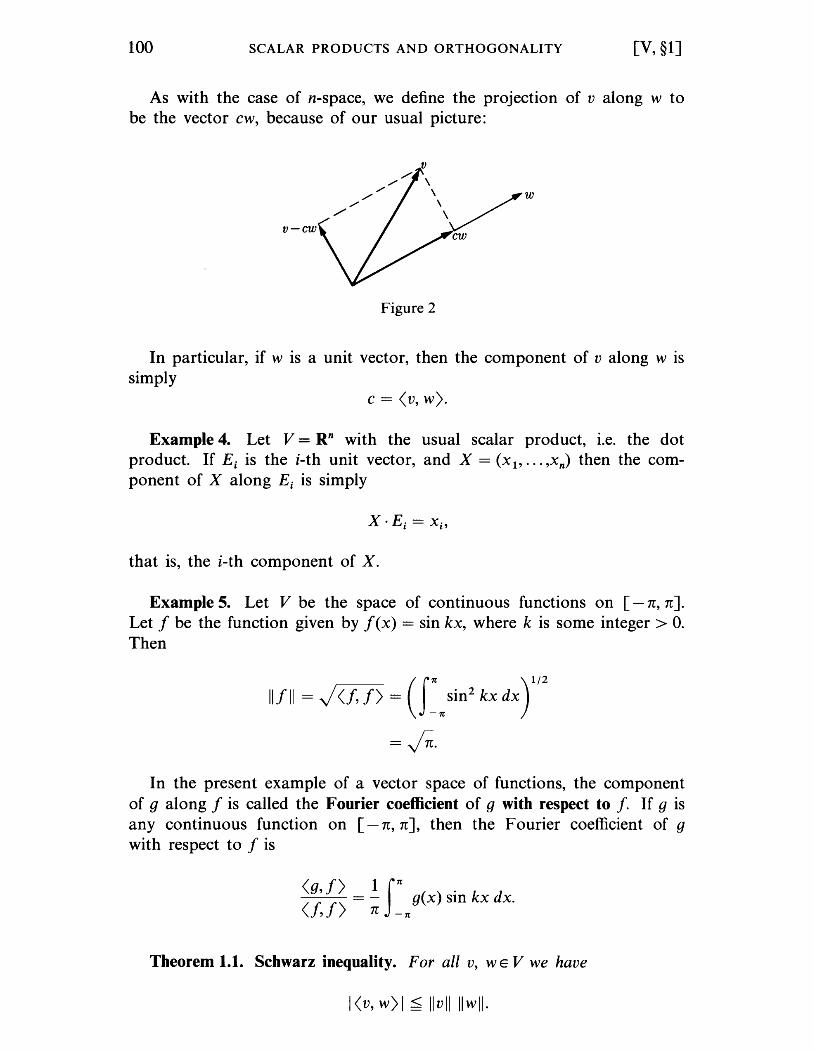
100 SCALAR PRODUCTS AND ORTHOGONALITY [V, §1]
As with the case of n-space, we define the projection of v along w to be the vector cw, because of our usual picture:
w
v-cw
Figure 2
In particular, if w is a unit vector, then the component of v along w is simply
c=<v,w).
Example 4. Let V = Rn with the usual scalar product, i.e. the dot product. If Ei is the i-th unit vector, and X = (Xl' ... ,xn) then the component of X along Ei is simply
that is, the i-th component of X.
Example 5. Let V be the space of continuous functions on [- n, n]. Let f be the function given by f(x) = sin kx, where k is some integer> O. Then
(f 1t )1/2 11111 = J <I,f) = -x sin
2 kx dx
=In. In the present example of a vector space of functions, the component
of g along f is called the Fourier coefficient of g with respect to f. If g is any continuous function on [- n, n], then the Fourier coefficient of g with respect to f is
<g, f) 1 f1t . k d <1,/) = -; -x g(x) SIll X x.
Theorem 1.1. Schwarz inequality. For all v, WE V we have
I <v, w) I < Ilvll Ilwll·
[V, §1] SCALAR PRODUCTS 101
Proof If w = 0, then both sides are equal to 0 and our inequality is obvious. Next, assume that w = e is a unit vector, that is e E V and Ilell = 1. If c is the component of v along e, then v - ce is perpendicular to e, and also perpendicular to ceo Hence by the Pythagoras theorem, we find
IIvl12 = Ilv - cel1 2 + IIce,,2
= "v - ce,,2 + c2.
Hence c2 < "vI1 2, so that Icl < IIvll. Finally, if w is arbitrary =f:. 0, then e = wj"w" is a unit vector, so that by what we just saw,
(v, 11:11) < Ilvll·
This yields
I <v, w) I < "vII IIwll,
as desired.
Theorem 1.2. Triangle inequality. If v, WE V, then
"v + w" < "v" + IIw".
Proof Each side of this inequality is positive or O. Hence it will suffice to prove that their squares satisfy the desired inequality, in other words
To do this we have:
(v + W)2 = (v + w)· (v + w) = v2 + 2v· w + w2
< IIvl1 2 + 211vll Ilwll + IIw211 (by Theorem 1.1)
= ("vII + IIwll)2,
thus proving the triangle inequality.
Let v1, ••• ,Vn be non-zero elements of V which are mutually perpendicular, that is <Vi' Vi) = 0 if i =f:. j. Let Ci be the component of v along Vi. Then
is perpendicular to v1, ••• ,vn • To see this, all we have to do is to take the product with vi for any j. All the terms involving <vi'Vi ) will give 0 if
102 SCALAR PRODUCTS AND ORTHOGONALITY [V, §1]
i i= j, and we shall have two remaining terms
which cancel. Thus subtracting linear combinations as above orthogonalizes v with respect to V 1, ••• ,Vn • The next theorem shows that c 1 v 1 + ... + cn Vn gives the closest approximation to v as a linear combination of v l' ... ,Vn •
Theorem 1.3. Let V 1, ••• ,Vn be vectors which are mutually perpendicular, and such that IIvill i= 0 for all i. Let v be an element of V, and let Ci be the component of v along Vi' Let a 1, •.. ,an be numbers. Then
Proof We know that
is perpendicular to each Vi' i = 1, ... ,no Hence it is perpendicular to any linear combination of V 1, ••• ,Vn • Now we have:
Ilv - L ak vk l12 = Ilv - L CkVk + L (Ck - ak )vk l1
2
= Ilv - L ck vk l12 + IlL (Ck - ak )vk l1
2
by the Pythagoras theorem. This proves that
and thus our theorem is proved.
The next theorem is known as the Bessel inequality.
Theorem 1.4. If V 1, ••• ,Vn are mutually perpendicular unit vectors, and if Ci is the component of v along Vi' then
n
L c1 < Ilv112. i= 1
[V, §2] ORTHOGONAL BASES, POSITIVE DEFINITE CASE 103
Proof The elements v - L CiVb Vb'" ,Vn are mutually perpendicular. Therefore:
IIvII2 = Ilv - L civdl 2 + ilL civill2
> ilL ci vi ll2
= Lcr
by Pythagoras
because a norm is > 0
by Pythagoras
because v1, ••• ,Vn are mutually perpendicular and IIvill2 = 1. This proves the theorem.
V, §1. EXERCISES
1. Let V be a vector space with a scalar product. Show that <0, v) = 0 for all v in V.
2. Assume that the scalar product is positive definite. Let Vi' ... ,vn be non-zero elements which are mutually perpendicular, that is <Vi' v j) = 0 if i '# j. Show that they are linearly independent.
3. Let M be a square n x n matrix which is equal to its transpose. If X, Yare column n-vectors, then
is a 1 x 1 matrix, which we identify with a number. Show that the map
(X, Y) ~ tXMY
satisfies the three properties SP 1, SP 2, SP 3. Give an example of a 2 x 2 matrix M such that the product is not positive definite.
V, §2. ORTHOGONAL BASES, POSITIVE DEFINITE CASE
Let V be a vector space with a positive definite scalar product throughout this section. A basis {v 1, ••• ,vn } of V is said to be orthogonal if its elements are mutually perpendicular, i.e. <Vi' Vj) = 0 whenever i i= j. If in addition each element of the basis has norm 1, then the basis is called orthonormal.
The standard unit vectors of Rn form an orthonormal basis of Rn, with respect to the ordinary dot product.
Theorem 2.1. Let V be a finite dimensional vector space, with a positive definite scalar product. Let W be a subspace of V, and let {w 1,.·· ,wm }
be an orthogonal basis of W If W i= V, then there exist elements wm + 1' ... ,Wn of V such that {w 1, .•• ,wn } is an orthogonal basis of v.
104 SCALAR PRODUCTS AND ORTHOGONALITY [V, §2]
Proof The method of proof is as important as the theorem, and is called the Gram-Schmidt orthogonalization process. We know from Chapter II, §3 that we can find elements vm + 1, ... ,vn of V such that
is a basis of V. Of course, it is not an orthogonal basis. Let W m + 1 be the space generated by W h ... ,Wm , Vm + 1. We shall first obtain an orthogonal basis of Wm + 1 • The idea is to take V m + 1 and substract from it its projection along W 1, ••• ,Wm • Thus we let
Let
Then W m + 1 is perpendicular to W 1, ••• , W m· Furthermore, W m + 1 =1= 0 (otherwise Vm + 1 would be linearly dependent on W 1, ••• ,W m), and Vm + 1 lies in the space generated by W h ... ,Wm + 1 because
Hence {w 1, ••• ,Wm + 1 } is an orthogonal basis of Wm + 1• We can now proceed by induction, showing that the space Wm + s generated by
has an orthogonal basis
with s = 1, ... ,n - m. This concludes the proof.
Corollary 2.2. Let V be a finite dimensional vector space with a positive definite scalar product. Assume that V -=1= {o}. Then V has an orthogonal basis.
Proof By hypothesis, there exists an element V 1 of V such that V 1 -=1= o. We let W be the subspace generated by Vb and apply the theorem to geOt the desired basis.
[V, §2] ORTHOGONAL BASES, POSITIVE DEFINITE CASE 105
We summarize the procedure of Theorem 2.1 once more. Suppose we are given an arbitrary basis {v 1, ••• ,vn } of V. We wish to orthogonalize it. We proceed as follows. We let
Then {V'1' ... ,v~} is an orthogonal basis.
Given an orthogonal basis, we can always obtain an orthonormal basis by dividing each vector by its norm.
Example 1. Find an orthonormal basis for the vector space generated by the vectors (1,1,0,1), (1, -2,0,0), and (1,0, -1,2).
Let us denote these vectors by A, B, C. Let
B·A B'=B--A.
A·A
In other words, we subtract from B its projection along A. Then B' is perpendicular to A. We find
B' = t(4, - 5, 0, 1).
Now we subtract from C its projection along A and B', and thus we let
C·A C·B' C' = C - - A - -- B'.
A·A B'·B'
Since A and B' are perpendicular, taking the scalar product of C' with A and B' shows that C' is perpendicular to both A and B'. We find
C' =~(-4, -2, -7,6).
The vectors A, B', C' are non-zero and mutually perpendicular. They lie in the space generated by A, B, C. Hence they constitute an orthogonal
106 SCALAR PRODUCTS AND ORTHOGONALITY [V, §2]
basis for that space. If we wish an orthonormal basis, then we divide these vectors by their norm, and thus obtain
A 1 -=-(1101) IIAII J3 ' , , , B' 1
IIB'II = j42(4, -5,0,1),
C' 1 IIC'II = jWs(-4, -2, -7,6),
as an orthonormal basis.
Theorem 2.3. Let V be a vector space over R with a positive definite scalar product, of dimension n. Let W be a subspace of V of dimension r. Let W-L be the subspace of V consisting of all elements which are perpendicular to W Then V is the direct sum of Wand W-L, and W-L has dimension n - r. In other words,
dim W + dim W-L = dim V.
Proof If W consists of 0 alone, or if W = V, then our assertion is obvious. We therefore assume that W =1= V and that W =1= {O}. Let {w 1, ••• ,wr } be an orthonormal basis of W By Theorem 2.1, there exist elements Ur + l' ... ,Un of V such that
is an orthonormal basis of V. We shall prove that {u r + 1' ... ,Un} is an orthonormal basis of W-L.
Let u be an element of W-L. Then there exist numbers Xl' ... ,xn such that
u = X1W 1 + ... + xrwr + xr+ 1ur+ 1 + ... + xnun.
Since u is perpendicular to W, taking the product with any Wi
(i = 1, ... ,r), we find
Hence all Xi = 0 (i = 1, ... ,r). Therefore u is a linear combination of ur + 1, ... ,Un·
Conversely, let u = Xr+ 1Ur+ 1 + ... + XnUn be a linear combination of ur+ 1, ... ,Un· Taking the product with any Wi yields o. Hence U is perpendicular to all Wi (i = 1, ... ,r), and hence is perpendicular to W This
[V, §2] ORTHOGONAL BASES, POSITIVE DEFINITE CASE 107
proves that Ur + b ... ,Un generate W1-. Since they are mutually perpendicular, and of norm 1, they form an orthonormal basis of W1-, whose dimension is therefore n - r. Furthermore, an element of V has a unique expression as a linear combination
and hence a unique expression as a sum W + U with WE Wand UE W1-. Hence V is the direct sum of Wand W 1-.
The space W 1- is called the orthogonal complement of W
Example 2. Consider R3. Let A, B be two linearly independent vectors in R3. Then the space of vectors which are perpendicular to both A and B is a I-dimensional space. If {N} is a basis for this space, any other basis for this space is of type {tN}, where t is a number i= o.
Again in R3, let N be a non-zero vector. The space of vectors perpen
dicular to N is a 2-dimensional space, i.e. a plane, passing through the origin O.
Let V be a finite dimensional vector space over R, with a posItIve definite scalar product. Let {e l , ... ,en} be an orthonormal basis. Let v, WE V. There exist numbers Xl' ... ,xnER and Yl' ... ,YnER such that
and
Then
n
= L xiYj<ei , e j) = XlYl + ... + XnYn· i,j= 1
Thus in terms of this orthonormal basis, if X, Yare the coordinate vectors of v and W respectively, the scalar product .is given by the ordinary dot product X· Y of the coordinate vectors. This is definitely not the case if we deal with a basis which is not orthonormal. If {v l , ... ,vn } is any basis of V, and we write
v = XlVl + ... + XnVn
W = YlV l + ... + YnVn
in terms of the basis, then
n
<v, W) = L XiYj<Vi, Vj). i,j= 1
108 SCALAR PRODUCTS AND ORTHOGONALITY
Hermitian products
n
<V, W) = L aijxixj , i,j= 1
[V, §2]
We shall now describe the modification necessary to adapt the preceding results to vector spaces over the complex numbers. We wish to preserve the notion of a positive definite scalar product as far as possible. Since the dot product of vectors with complex coordinates may be equal to 0 without the vectors being equal to 0, we must change something in the definition. It turns out that the needed change is very slight.
Let V be a vector space over the complex numbers. A hermitian product on V is a rule which to any pair of elements V, W of V associates a complex number, denoted again by <v, w), satisfying the following properties:
HP 1. We have <v, w) = <w, v) for all v, WE V. (Here the bar denotes complex conjugate.)
HP 2. If u, v, ware elements of V, then
< u, v + w) = < u, v) + < u, w).
HP 3. If aEC, then
<au,v) = (x<u,v) and <u, (Xv) = a<u, v).
The hermitian product is said to be positive definite if < v, v) > 0 for all v E V, and < v, v) > 0 if v i= 0.
We define the words orthogonal, perpendicular, orthogonal basis, orthogonal complement as before. There is nothing to change either in our definition of component and projection of v along w, or in the remarks which we made concerning these.
Example 3. Let V = cn. If X = (x b ... ,xn) and Y = (Yl"" ,Yn) are vectors in Cn
, we define their hermitian product to be
Conditions HP 1, HP 2 and HP 3 are immediately verified. This product is positive definite because if X i= 0, then some Xi i= 0, and XiXi > O. Hence <X, X) > O.
[V, §2] ORTHOGONAL BASES, POSITIVE DEFINITE CASE 109
Note however that if X = (1, i) then
X·X = 1 - 1 = o.
Example 4. Let V be the space of continuous complex-valued functions on the interval [ - n, n]. If j, g E V, we define
<I. g) = f/(t)g(t) dt.
Standard properties of the integral again show that this is a hermitian product which is positive definite. Let fn be the function such that
A simple computation shows that fn is orthogonal to f m if n, m are distinct integers. Furthermore, we have
If f E V, then its Fourier coefficient with respect to fn is therefore equal to
which a reader acquainted with analysis will immediately recognize.
We return to our general discussion of hermitian products. We have the analogue of Theorem 2.1 and its corollary for positive definite hermitian products, namely:
Theorem 2.4. Let V be a finite dimensional vector space over the complex numbers, with a positive definite hermitian product. Let W be a subspace of V, and let {w 1, ••• ,wm } be an orthogonal basis of W. If W i= V, then there exist elements w m + l' ••• , W n of V such that {w 1, ••• ,wn} is an orthogonal basis of V.
Corollary 2.5. Let V be a finite dimensional vector space over the complex numbers, with a positive definite hermitian product. Assume that V i= {O}. Then V has an orthogonal basis.
The proofs are exactly the same as those given previously for the real case, and there is no need to repeat them.
110 SCALAR PRODUCTS AND ORTHOGONALITY [V, §2]
We now come to the theory of the norm. Let V be a vector space over C, with a positive definite hermitian product. If v E V, we define its norm by letting
Ilvll = J <v, v).
Since <v, v) is real, > 0, its square root is taken as usual to be the unique real number > 0 whose square is <v, v).
We have the Schwarz inequality, namely
I<v, w)1 < IIvll Ilwll·
The three properties of the norm hold as in the real case:
For all VE V, we have Ilvll > 0, and = 0 if and only if v = o.
For any complex number a, we have Ilavll = lal Ilvll.
For any elements v, WE V we have Ilv + wll < Ilvll + Ilwll.
All these are again easily verified. We leave the first two as exercises, and carry out the third completely, using the Schwarz inequality.
I t will suffice to prove that
To do this, we observe that
Ilv + wl1 2 = <v + w,v + w) = <v, v) + <w, v) + <v, w) + <w, w).
But <w, v) + <v, w) = <v, w) + <v, w) < 21<v, w)l. Hence by Schwarz,
Ilv + wl12 < IIvl12 + 21<v, w)1 + IIwl12
< IIvl12 + 211vll Ilwll + IIwl12 = (11vll + IIwll)2.
Taking the square root of each side yields what we want.
An element v of V is said to be a unit vector as in the real case, if II vii = 1. An orthogonal basis {v l , ... ,vn} is said to be orthonormal if it consists of unit vectors. As before, we obtain an orthonormal basis from an orthogonal one by dividing each vector by its norm.
Let {e l' ... ,en} be an orthonormal basis of V. Let v, WE V. There exist complex numbers a l , ... ,an E C and Pl' ... ,Pn E C such that
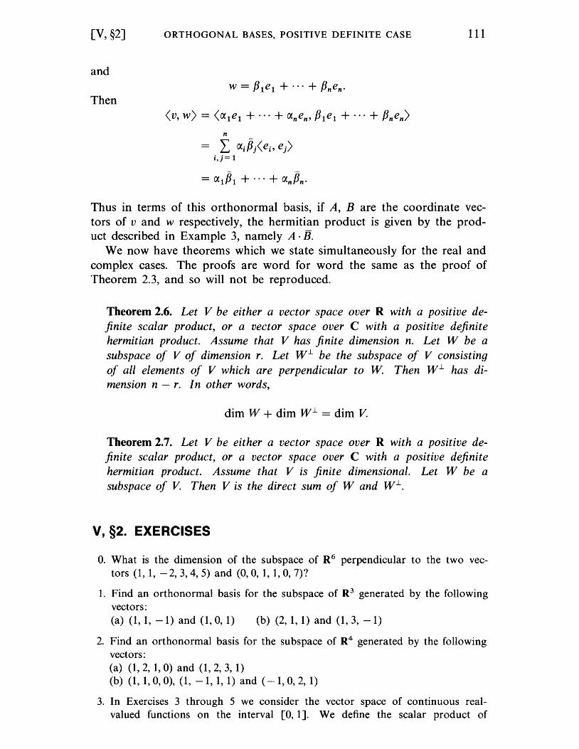
[V, §2]
and
Then
ORTHOGONAL BASES, POSITIVE DEFINITE CASE
n
= L aiPj<ei, ej) i,j= 1
- -= alPl + ... + anPn·
111
Thus in terms of this orthonormal basis, if A, B are the coordinate vectors of v and w respectively, the hermitian product is given by the product described in Example 3, namely A· B.
We now have theorems which we state simultaneously for the real and complex cases. The proofs are word for word the same as the proof of rfheorem 2.3, and so will not be reproduced.
Theorem 2.6. Let V be either a vector space over R with a positive de-finite scalar product, or a vector space over C with a positive definite hermitian product. Assume that V has finite dimension n. Let W be a subspace of V of dimension r. Let W1- be the subspace of V consisting of all elements of V which are perpendicular to W. Then W 1- has dimension n - r. In other words,
dim W + dim W1- = dim V.
Theorem 2.7. Let V be either a vector space over R with a positive definite scalar product, or a vector space over C with a positive definite hermitian product. Assume that V is finite dimensional. Let W be a subspace of V. Then V is the direct sum of Wand W1-.
V, §2. EXERCISES
0. What is the dimension of the subspace of R 6 perpendicular to the two vectors (1, 1, - 2, 3,4, 5) and (0,0, 1, 1,0, 7)?
1. Find an orthonormal basis for the subspace of R 3 generated by the following vectors: (a) (1, 1, -1) and (1, 0, 1) (b) (2,1,1) and (1,3, -1)
2. Find an orthonormal basis for the subspace of R4 generated by the following vectors: (a) (1,2,1,0) and (1,2,3,1) (b) (1,1,0,0), (1, -1,1,1) and (-1,0,2,1)
3. In Exercises 3 through 5 we consider the vector space of continuous realvalued functions on the interval [0, 1J. We define the scalar product of
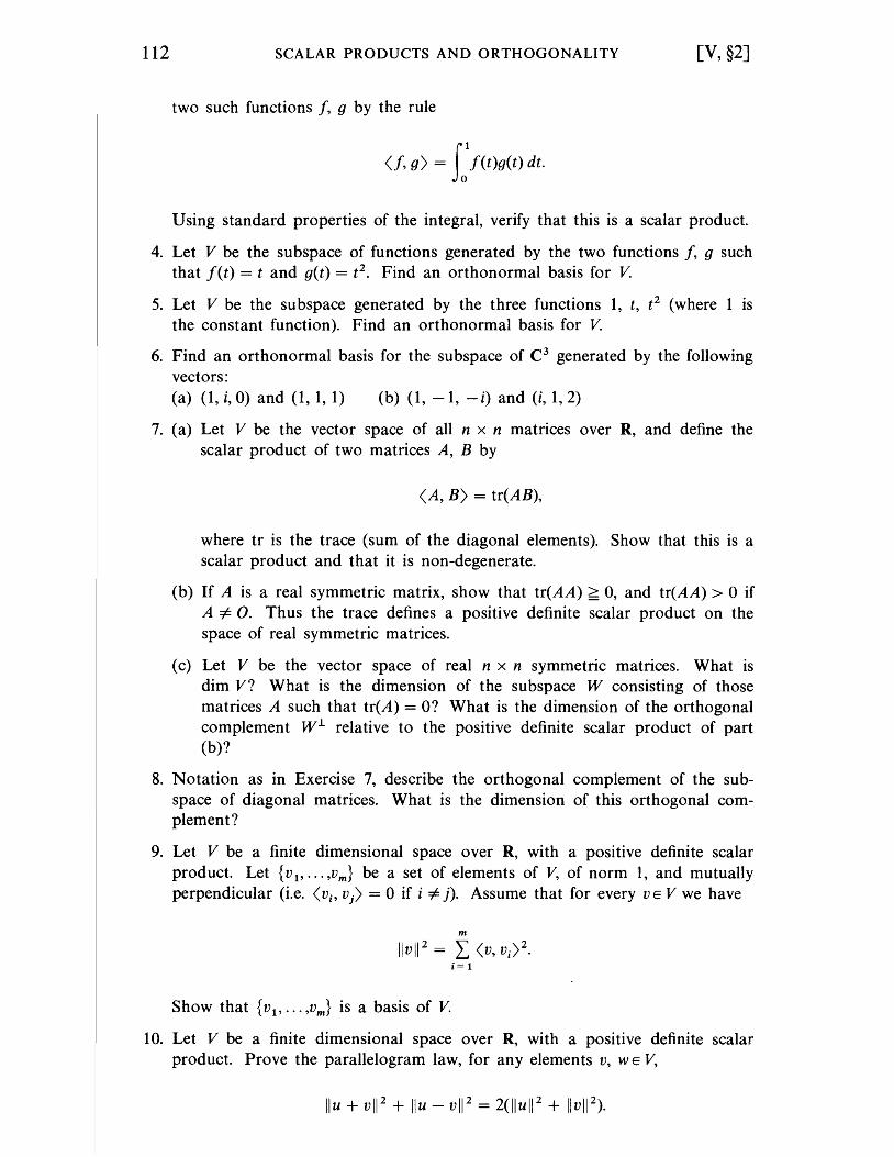
112 SCALAR PRODUCTS AND ORTHOGONALITY [V, §2]
two such functions j, g by the rule
<I, g) = ff(t)g(t) dt.
Using standard properties of the integral, verify that this is a scalar product.
4. Let V be the subspace of functions generated by the two functions j, g such that Jet) = t and get) = t2
• Find an orthonormal basis for V.
5. Let V be the subspace generated by the three functions 1, t, t 2 (where 1 is the constant function). Find an orthonormal basis for V.
6. Find an orthonormal basis for the subspace of C 3 generated by the following vectors: (a) (1, i,O) and (1, 1, 1) (b) (1, -1, - i) and (i, 1, 2)
7. (a) Let V be the vector space of all n x n matrices over R, and define the scalar product of two matrices A, B by
(A, B) = tr(AB),
where tr is the trace (sum of the diagonal elements). Show that this is a scalar product and that it is non-degenerate.
(b) If A is a real symmetric matrix, show that tr(AA) ~ 0, and tr(AA) > 0 if A ¥= O. Thus the trace defines a positive definite scalar product on the space of real symmetric matrices.
( c) Let V be the vector space of real n x n symmetric matrices. What is dim V? What is the dimension of the subspace W consisting of those matrices A such that tr(A) = O? What is the dimension of the orthogonal complement W.l relative to the positive definite scalar product of part (b)?
8. Notation as in Exercise 7, describe the orthogonal complement of the subspace of diagonal matrices. What is the dimension of this orthogonal complement?
9. Let V be a finite dimensional space over R, with a positive definite scalar product. Let {v l' ... ,vm } be a set of elements of V, of norm 1, and mutually perpendicular (i.e. (Vi' Vj ) = 0 if i ¥= j). Assume that for every V E V we have
m
IIvI12 = L (v, Vi )2. i= 1
Show that {V l' ... ,Vm } is a basis of V.
10. Let V be a finite dimensional space over R, with a posItIve definite scalar product. Prove the parallelogram law, for any elements v, WE V,
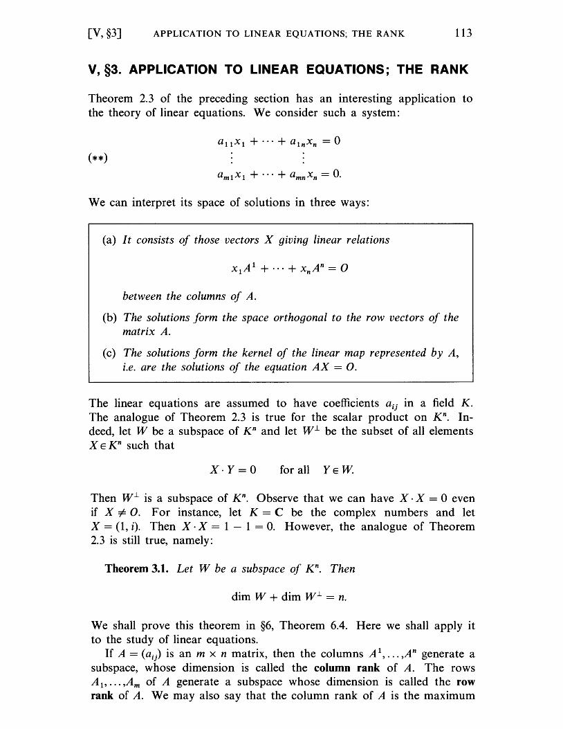
[V, §3] APPLICATION TO LINEAR EQUATIONS; THE RANK 113
V, §3. APPLICATION TO LINEAR EQUATIONS; THE RANK
Theorem 2.3 of the preceding section has an interesting application to the theory of linear equations. We consider such a system:
We can interpret its space of solutions in three ways:
(a) It consists of those vectors X giving linear relations
between the columns of A.
(b) The solutions form the space orthogonal to the row vectors of the matrix A.
(c) The solutions form the kernel of the linear map represented by A, i.e. are the solutions of the equation AX = o.
The linear equations are assumed to have coefficients aij in a field K. The analogue of Theorem 2.3 is true for the scalar product on Kn. Indeed, let W be a subspace of K n and let W1- be the subset of all elements X E K n such that
X·Y=O for all YEW
Then W1- is a subspace of Kn. Observe that we can have X· X = 0 even if X i= O. For instance, let K = C be the complex numbers and let X = (1, i). Then X· X = 1 - 1 = O. However, the analogue of Theorem 2.3 is still true, namely:
Theorem 3.1. Let W be a subspace of Kn. Then
dim W + dim W 1- = n.
We shall prove this theorem in §6, Theorem 6.4. Here we shall apply it to the study of linear equations.
If A = (aij) is an m x n matrix, then the columns A 1, ... ,An generate a subspace, whose dimension is called the column rank of A. The rows A l , ... ,Am of A generate a subspace whose dimension is called the row rank of A. We may also say that the column rank of A is the maximum
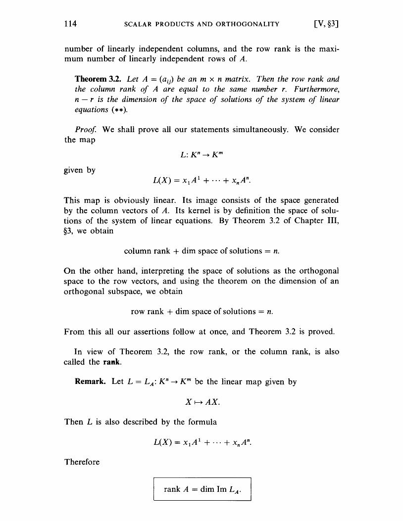
114 SCALAR PRODUCTS AND ORTHOGONALITY [V, §3]
number of linearly independent columns, and the row rank is the maximum number of linearly independent rows of A.
Theorem 3.2. Let A = (a ij) be an m x n matrix. Then the row rank and the column rank of A are equal to the same number r. Furthermore, n - r is the dimension of the space of solutions of the system of linear equations (* * ).
Proof We shall prove all our statements simultaneously. We consider the map
given by
This map is obviously linear. Its image consists of the space generated by the column vectors of A. Its kernel is by definition the space of solutions of the system of linear equations. By Theorem 3.2 of Chapter III, §3, we obtain
column rank + dim space of solutions = n.
On the other hand, interpreting the space of solutions as the orthogonal space to the row vectors, and using the theorem on the dimension of an orthogonal subspace, we obtain
row rank + dim space of solutions = n.
From this all our assertions follow at once, and Theorem 3.2 is proved.
In view of Theorem 3.2, the row rank, or the column rank, is also called the rank.
Remark. Let L = LA: K n ---+ K m be the linear map given by
X~AX.
Then L is also described by the formula
Therefore
rank A = dim 1m LA.
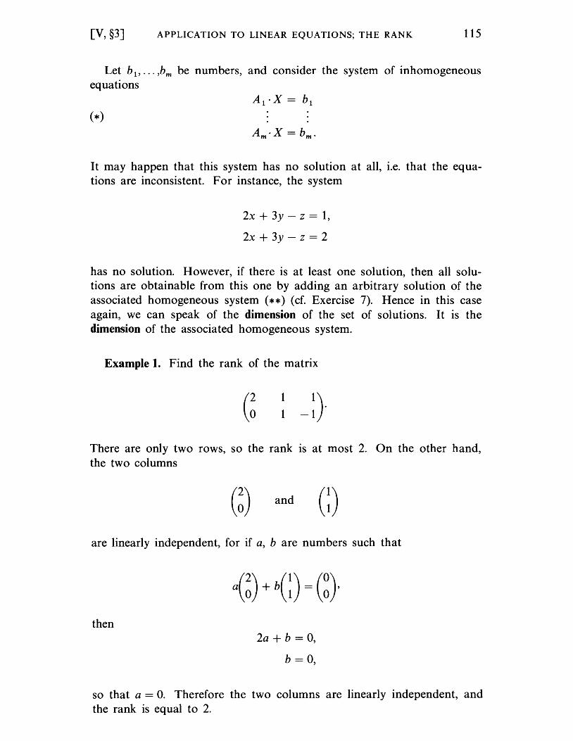
[V, §3] APPLICATION TO LINEAR EQUATIONS; THE RANK 115
Let bi , ... ,bm be numbers, and consider the system of inhomogeneous equations
It may happen that this system has no solution at all, i.e. that the equations are inconsistent. For instance, the system
2x + 3y - z = 1,
2x + 3y - z = 2
has no solution. However, if there is at least one solution, then all solutions are obtainable from this one by adding an arbitrary solution of the associated homogeneous system (**) (cf. Exercise 7). Hence in this case again, we can speak of the dimension of the set of solutions. It is the dimension of the associated homogeneous system.
Example 1. Find the rank of the matrix
(~ 1
1
There are only two rows, so the rank is at most 2. On the other hand, the two columns
(~) and G) are linearly independent, for if a, b are numbers such that
then 2a + b = 0,
b = 0,
so that a = 0. Therefore the two columns are linearly independent, and the rank is equal to 2.
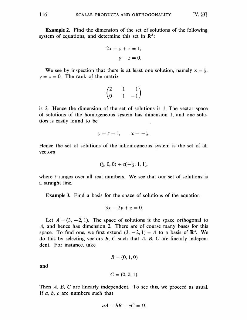
116 SCALAR PRODUCTS AND ORTHOGONALITY [V, §3]
Example 2. Find the dimension of the set of solutions of the following system of equations, and determine this set in R3:
2x + y + z = 1,
y - z = o.
We see by inspection that there is at least one solution, namely x = t, y = z = O. The rank of the matrix
(~ 1
1
is 2. Hence the dimension of the set of solutions is 1. The vector space of solutions of the homogeneous system has dimension 1, and one solution is easily found to be
y = z = 1, x = -to
Hence the set of solutions of the inhomogneous system is the set of all vectors
(t, 0, 0) + t( -t, 1, 1),
where t ranges over all real numbers. We see that our set of solutions is a straight line.
Example 3. Find a basis for the space of solutions of the equation
3x - 2y + z = O.
Let A = (3, - 2, 1). The space of solutions is the space orthogonal to A, and hence has dimension 2. There are of course many bases for this space. To find one, we first extend (3, -2,1) = A to a basis of R3. We do this by selecting vectors B, C such that A, B, C are linearly independent. For instance, take
B = (0, 1, 0)
and
C = (0,0, 1).
Then A, B, C are linearly independent. To see this, we proceed as usual. If a, b, c are numbers such that
aA + bB + cC = 0,
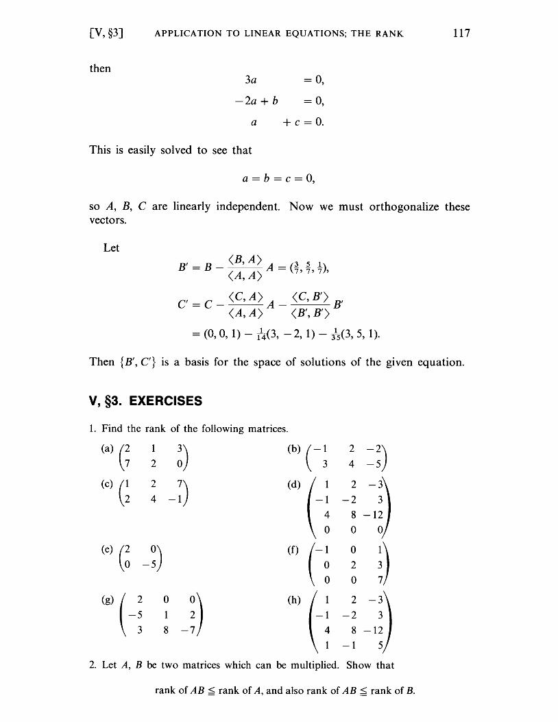
[V, §3] APPLICATION TO LINEAR EQUATIONS; THE RANK 117
then 3a = 0,
-2a + b = 0,
a + c = 0.
This is easily solved to see that
a = b = c = 0,
so A, B, C are linearly independent. Now we must orthogonalize these vectors.
Let
B' = B _ (B, A) A = (~ ~ ~) (A, A) 7' 7' 7 ,
C' = C _ (C, A) A _ (C, B') B' (A, A) (B', B')
= (0,0, 1) - l4(3, - 2, 1) - ls(3, 5, 1).
Then {B', C'} is a basis for the space of solutions of the given equation.
V, §3. EXERCISES
1. Find the rank of the following matrices.
(a) G 1
~) (b) (- ~ 2 -2) 2 4 -5
(c) G "" -;) (d) 1 2 -3 ~
4 -1 -2 3 4 8 -12
0 0 0
(e) G -~) (f)
(-~ 0
~) 2
0
(g) ( -: 0
-D (h) 1 2 -3
1 -1 -2 3 8 4 8 -12
1 -1 5
2. Let A, B be two matrices which can be multiplied. Show that
rank of AB ~ rank of A, and also rank of AB ~ rank of B.
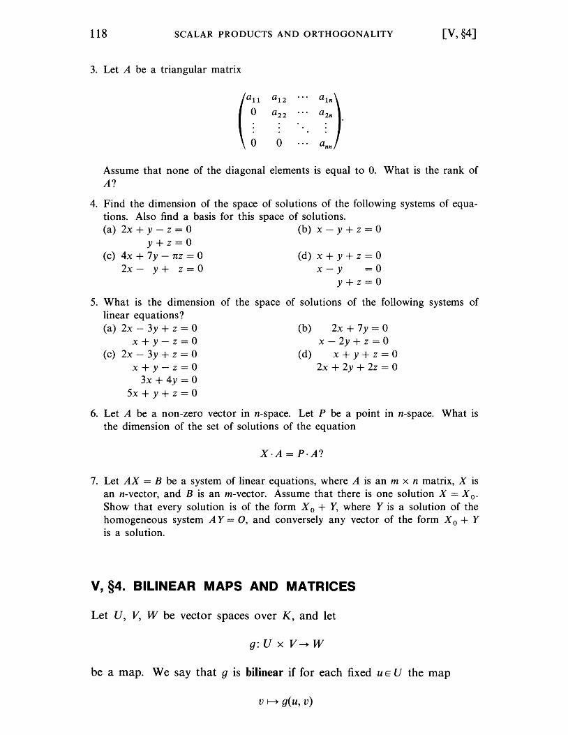
118 SCALAR PRODUCTS AND ORTHOGONALITY [V, §4]
3. Let A be a triangular matrix
Assume that none of the diagonal elements is equal to O. What is the rank of A?
4. Find the dimension of the space of solutions of the following systems of equations. Also find a basis for this space of solutions. (a) 2x + y - z = 0 (b) x - y + z = 0
y+z=O (c) 4x + 7y - nz = 0
2x- y+ z=O (d) x + y + z = 0
x-y =0 y+z=O
5. What is the dimension of the space of solutions of the following systems of linear equations? (a) 2x - 3y + z = 0
x+y-z=O (c) 2x - 3y + z = 0
x+y-z=O 3x + 4y = 0
5x + y + z = 0
(b) 2x + 7y = 0 x - 2y + z = 0
(d) x + y + z = 0 2x + 2y + 2z = 0
6. Let A be a non-zero vector in n-space. Let P be a point in n-space. What is the dimension of the set of solutions of the equation
X·A=P·A?
7. Let AX = B be a system of linear equations, where A is an m x n matrix, X is an n-vector, and B is an m-vector. Assume that there is one solution X = X o. Show that every solution is of the form X 0 + Y, where Y is a solution of the homogeneous system A Y = 0, and conversely any vector of the form X 0 + y is a solution.
V, §4. BILINEAR MAPS AND MATRICES
Let U, V, W be vector spaces over K, and let
g: U x V ---+ W
be a map. We say that g is bilinear if for each fixed U E U the map
v ~ g(u, v)
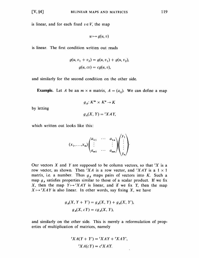
[V, §4] BILINEAR MAPS AND MATRICES
is linear, and for each fixed v E V, the map
u ~ g(U, v)
is linear. The first condition written out reads
g(u, VI + V2) = g(U, VI) + g(U, V2),
g(U, CV) = cg(U, V),
and similarly for the second condition on the other side.
119
Example. Let A be an m x n matrix, A = (aij). We can define a map
by letting
which written out looks like this:
YI Cll a~n ) (xI,···,xm) :
amI amn Yn
Our vectors X and Yare supposed to be column vectors, so that tx is a row vector, as shown. Then tXA is a row vector, and tXAY is a 1 x 1 matrix, i.e. a number. Thus gA maps pairs of vectors into K. Such a map gA satisfies properties similar to those of a scalar product. If we fix X, then the map y~tXAY is linear, and if we fix Y, then the map X ~ tXAY is also linear. In other words, say fixing X, we have
gA(X, Y + Y') = gA(X, Y) + gA(X, Y'),
gA(X, cY) = cgA(X, Y),
and similarly on the other side. This is merely a reformulation of properties of multiplication of matrices, namely
tXA(Y + Y') = tXAY + tXAY',
tXA(cY) = ctXAY.
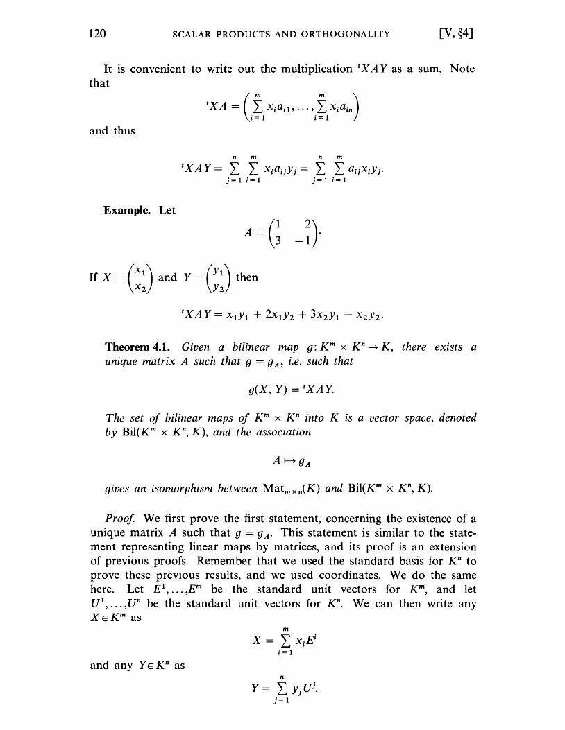
120 SCALAR PRODUCTS AND ORTHOGONALITY [V, §4]
It is convenient to write out the multiplication tx A Y as a sum. Note that
and thus
n m n m
tXAY= L L xiaijYj = L L aijxiYj· j=l i=l j=l i=l
Example. Let
A = G -~} If X = G:) and Y = G:) then
Theorem 4.1. Given a bilinear map g: K m x Kn -+ K, there exists a unique matrix A such that g = g A' i.e. such that
g(X, Y) = tXAY.
The set of bilinear maps of Km x Kn into K is a vector space, denoted by Bil(Km x Kn, K), and the association
gives an isomorphism between Matm x n(K) and Bil(Km x K n, K).
Proof. We first prove the first statement, concerning the existence of a unique matrix A such that g = g A. This statement is similar to the statement representing linear maps by matrices, and its proof is an extension of previous proofs. Remember that we used the standard basis for Kn to prove these previous results, and we used coordinates. We do the same here. Let E 1
, ••• ,Em be the standard unit vectors for K m, and let ui, ... ,un be the standard unit vectors for Kn. We can then write any XEKm as
and any Y E Kn as
m
n
Y= LyjUj.
j= 1
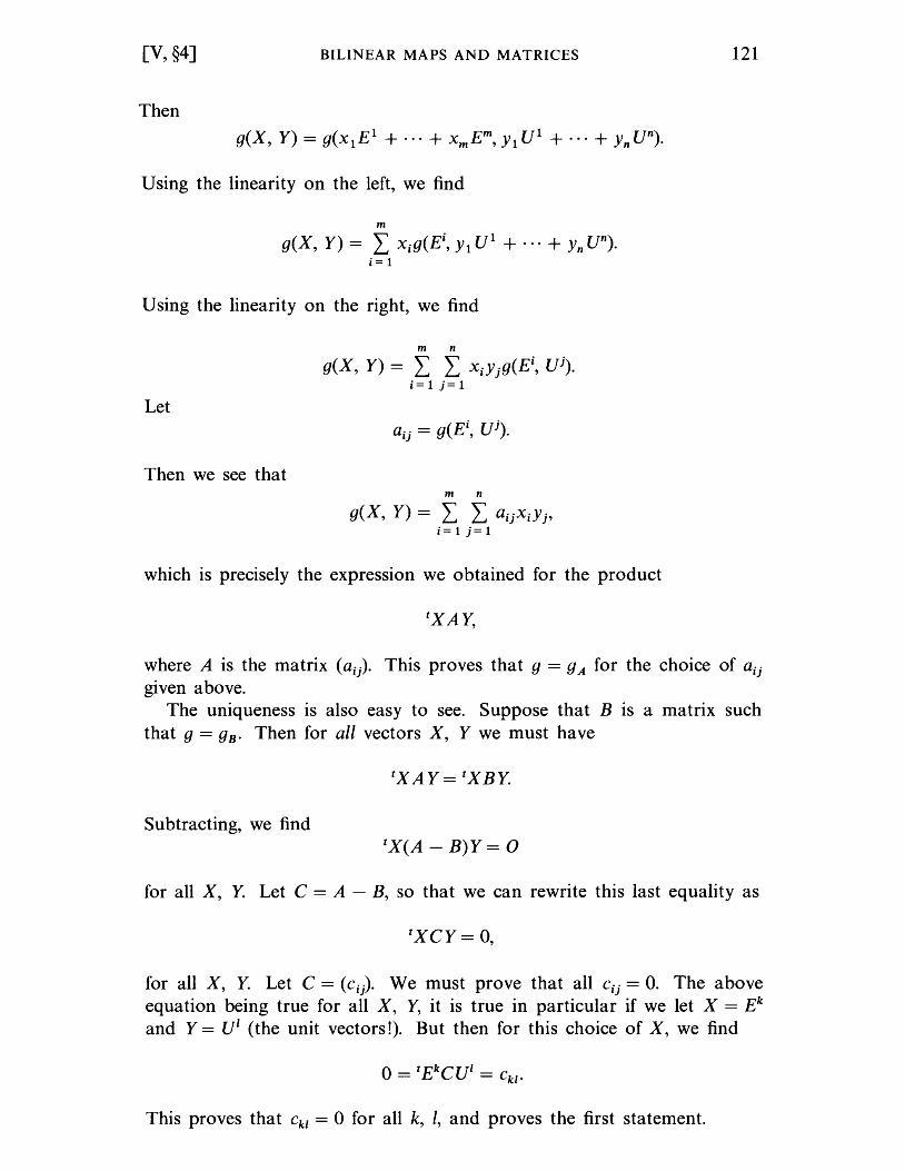
[V, §4] BILINEAR MAPS AND MATRICES 121
Then
g(X, Y) = g(x1E1 + ... + xmEm, Y1 U 1 + ... + Yn un).
U sing the linearity on the left, we find
m
g(X, Y) = L xig(Ei, Y1 U 1 + ... + Yn un). i= 1
U sing the lineari ty on the right, we find
m n
g(X, Y) = L L xiYjg(Ei, U j). i=1 j=1
Let
Then we see that m n
g(X, Y) = L L aijxiYj, i=1 j=1
which is precisely the expression we obtained for the product
tXAY,
where A is the matrix (aij). This proves that g = gA for the choice of aij given above.
The uniqueness is also easy to see. Suppose that B is a matrix such that g = gR. Then for all vectors X, Y we must have
Subtracting, we find tX(A - B)Y= 0
for all X, Y. Let C = A - B, so that we can rewrite this last equality as
for all X, Y. Let C = (c ij). We must prove that all cij = O. The above equation being true for all X, Y, it is true in particular if we let X = Ek and Y = U' (the unit vectors!). But then for this choice of X, we find
This proves that Ckl = 0 for all k, I, and proves the first statement.
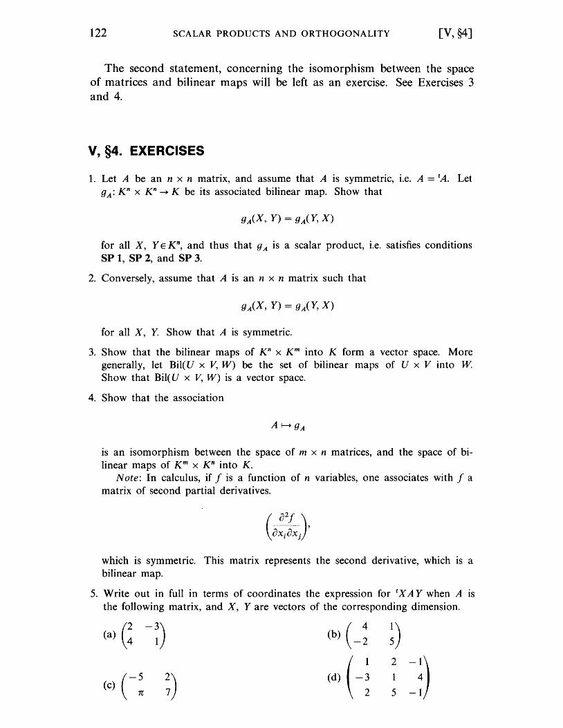
122 SCALAR PRODUCTS AND ORTHOGONALITY [V, §4]
The second statement, concerning the isomorphism between the space of matrices and bilinear maps will be left as an exercise. See Exercises 3 and 4.
V, §4. EXERCISES
1. Let A be an n x n matrix, and assume that A is symmetric, i.e. A = tAo Let g A: K n x K n --+ K be its associated bilinear map. Show that
for all X, Y E K n, and thus that g A is a scalar product, i.e. satisfies conditions
SP 1, SP 2, and SP 3.
2. Conversely, assume that A is an n x n matrix such that
for all X, Y. Show that A is symmetric.
3. Show that the bilinear maps of K n x K m into K form a vector space. More generally, let Bil(U x V, W) be the set of bilinear maps of U x V into W. Show that Bil( U x V, W) is a vector space.
4. Show that the association
is an isomorphism between the space of m x n matrices, and the space of bilinear maps of K m x Kn into K.
Note: In calculus, if f is a function of n variables, one associates with f a matrix of second partial derivatives.
which is symmetric. This matrix represents the second derivative, which is a bilinear map.
5. Write out in full in terms of coordinates the expression for tx A Y when A IS
the following matrix, and X, Yare vectors of the corresponding dimension.
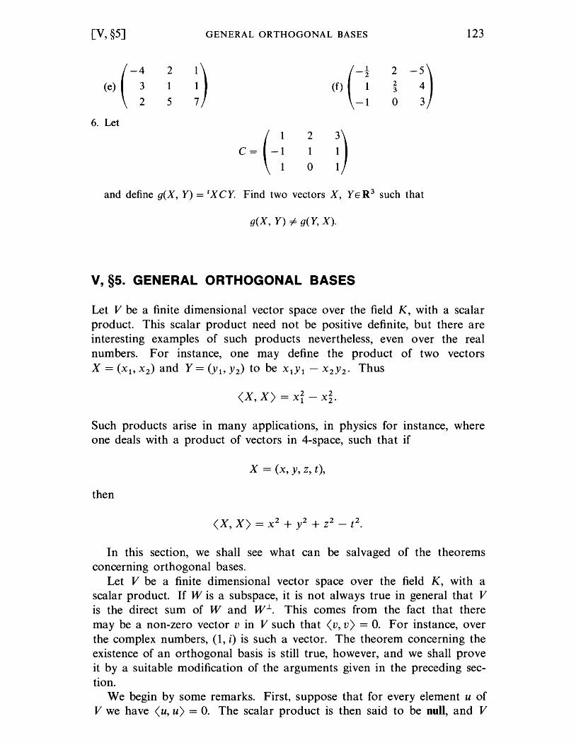
[V, §5] GENERAL ORTHOGONAL BASES 123
(e) ( -~ 2
D (f) (-~ 2 -n 1 2 "3
5 -1 0
6. Let
c= (-:
2
D 1
0
and define g(X, Y) = tXCY. Find two vectors X, YER 3 such that
g(X, Y) :;6 g(Y, X).
V, §5. GENERAL ORTHOGONAL BASES
Let V be a finite dimensional vector space over the field K, with a scalar product. This scalar product need not be positive definite, but there are interesting examples of such products nevertheless, even over the real numbers. For instance, one may define the product of two vectors X = (Xl' X2) and Y = (Yl' Y2) to be XlYl - X2Y2. Thus
Such products arise in many applications, in physics for instance, where one deals with a product of vectors in 4-space, such that if
x = (x, y, z, t),
then
In this section, we shall see what can be salvaged of the theorems concerning orthogonal bases.
Let V be a finite dimensional vector space over the field K, with a scalar product. If W is a subspace, it is not always true in general that V is the direct sum of Wand Wl.. This comes from the fact that there may be a non-zero vector v in V such that (v, v) = O. For instance, over the complex numbers, (1, i) is such a vector. The theorem concerning the existence of an orthogonal basis is still true, however, and we shall prove it by a suitable modification of the arguments given in the preceding section.
We begin by some remarks. First, suppose that for every element u of V we have (u, u) = O. The scalar product is then said to be null, and V
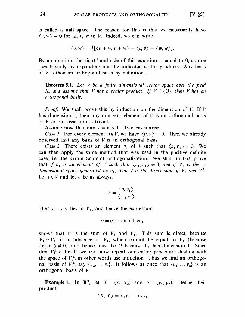
124 SCALAR PRODUCTS AND ORTHOGONALITY [V, §5]
is called a null space. The reason for this is that we necessarily have (v, w) = 0 for all v, w in V. Indeed, we can write
(v, w) = ![(v + w, v + w) - (v, v) - (w, w)].
By assumption, the right-hand side of this equation is equal to 0, as one sees trivially by expanding out the indicated scalar products. Any basis of V is then an orthogonal basis by definition.
Theorem 5.1. Let V be a finite dimensional vector space over the field K, and assume that V has a scalar product. If V i= {O}, then V has an orthogonal basis.
Proof We shall prove this by induction on the dimension of V. If V has dimension 1, then any non-zero element of V is an orthogonal basis of V so our assertion is trivial.
Assume now that dim V = n > 1. Two cases arise. Case 1. For every element UE V, we have (u, u) = O. Then we already
observed that any basis of V is an orthogonal basis. Case 2. There exists an element V l of V such that (Vl vl ) i= O. We
can then apply the same method that was used in the positive definite case, i.e. the Gram-Schmidt orthogonalization. We shall in fact prove that if V l is an element of V such that (Vb V l ) i= 0, and if Vl is the 1-dimensional space generated by Vl' then V is the direct sum of Vl and vt. Let v E V and let c be as always,
Then v - CV l lies in vt, and hence the expression
shows that V is the sum of Vl and V~. This sum is direct, because Vl n vt is a subspace of Vb which cannot be equal to V1 (because (Vl' Vl) i= 0), and hence must be 0 because V1 has dimension 1. Since dim vt < dim V, we can now repeat our entire procedure dealing with the space of vt, in other words use induction. Thus we find an orthogonal basis of V~, say {v 2 , ••• ,vn}. It follows at once that {v 1, .•• ,vn } is an orthogonal basis of V.
Example 1. In R2, let X = (Xb x 2) and Y = (Yb Y2). Define their product
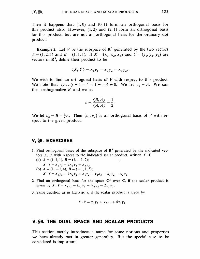
[V, §6] THE DUAL SPACE AND SCALAR PRODUCTS 125
Then it happens that (1, 0) and (0, 1) form an orthogonal basis for this product also. However, (1, 2) and (2, 1) form an orthogonal basis for this product, but are not an orthogonal basis for the ordinary dot product.
Example 2. Let V be the subspace of R3 generated by the two vectors A = (1, 2, 1) and B = (1, 1, 1). If X = (Xl' X 2, x 3) and Y = (Yl' Y2' Y3) are vectors in R 3, define their product to be
We wish to find an orthogonal basis of V with respect to this product. We note that <A, A) = 1 - 4 - 1 = -4 i= O. We let V l = A. We can then orthogonalize B, and we let
<B, A) 1 c = =-.
<A, A) 2
We let V 2 = B - tAo Then {Vl' v2 } is an orthogonal basis of V with respect to the given product.
V, §5. EXERCISES
1. Find orthogonal bases of the subspace of R 3 generated by the indicated vectors A, B, with respect to the indicated scalar product, written X· Y. (a) A = (1, 1, 1), B = (1, - 1, 2);
X· Y = XtYt + 2X2 Y2 + X 3 Y3
(b) A = (1, - 1, 4), B = ( - 1, 1, 3); X· Y = XtYt - 3X2 Y2 + X t Y3 + Yt X 3 - X 3 Y2 - X 2 Y3
2. Find an orthogonal base for the space C2 over C, if the scalar product IS
given by X· Y = XtYt - iX 2 Yt - iX t Y2 - 2X 2 Y2.
3. Same question as in Exercise 2, if the scalar product is given by
V, §6. THE DUAL SPACE AND SCALAR PRODUCTS
This section merely introduces a name for some notions and properties we have already met in greater generality. But the special case to be considered is important.
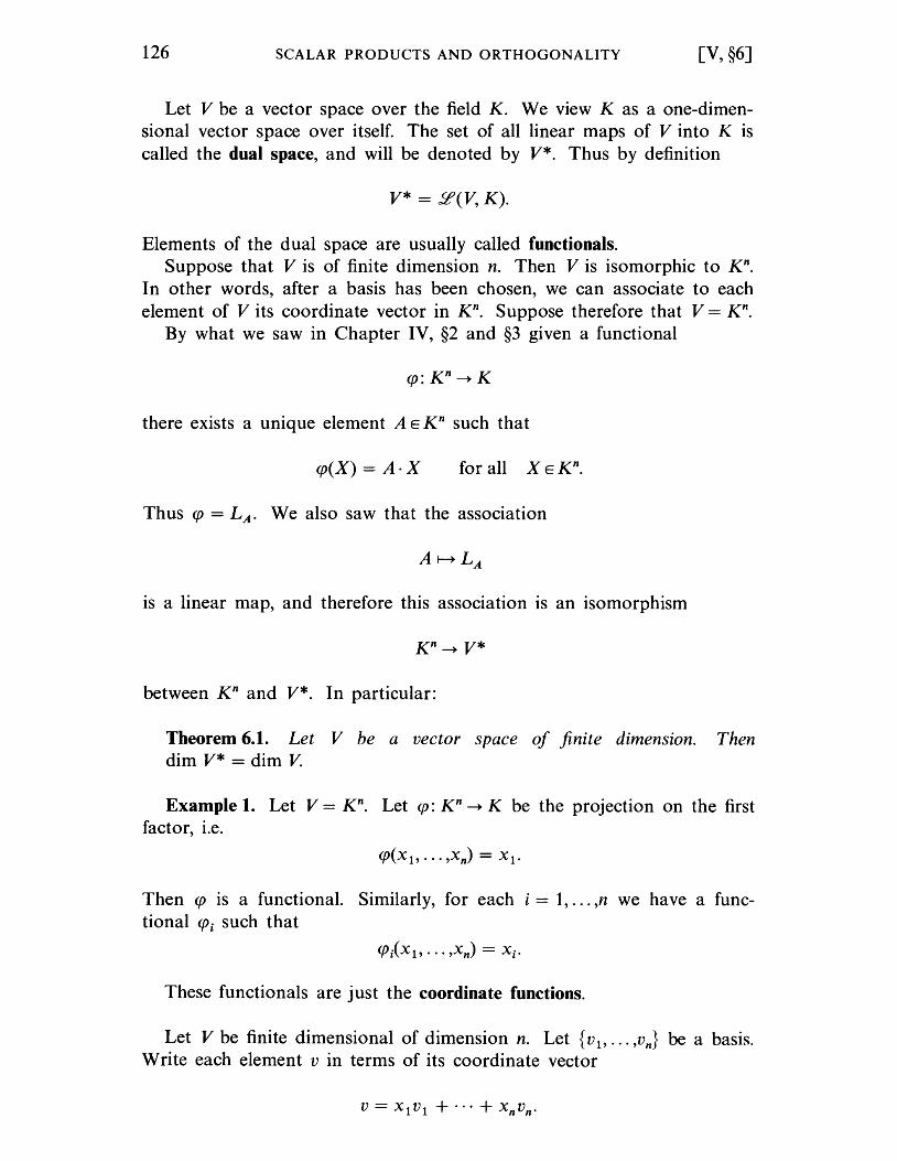
126 SCALAR PRODUCTS AND ORTHOGONALITY [V, §6]
Let V be a vector space over the field K. We view K as a one-dimensional vector space over itself. The set of all linear maps of V into K is called the dual space, and will be denoted by V*. Thus by definition
V* = !l'(V, K).
Elements of the dual space are usually called functionals. Suppose that V is of finite dimension n. Then V is isomorphic to Kn.
In other words, after a basis has been chosen, we can associate to each element of V its coordinate vector in Kn. Suppose therefore that V = Kn.
By what we saw in Chapter IV, §2 and §3 given a functional
there exists a unique element A E K n such that
qJ(X) = A·X
Thus qJ = LA. We also saw that the association
is a linear map, and therefore this association is an isomorphism
between K n and V*. In particular:
Theorem 6.1. Let V be a vector space of finite dimension. Then dim V* = dim V.
Example 1. Let V = Kn. Let qJ: K n -+ K be the projection on the first factor, i.e.
Then qJ is a functional. Similarly, for each i = 1, ... ,n we have a functional qJi such that
These functionals are just the coordinate functions.
Let V be finite dimensional of dimension n. Let {v 1, ••• ,vn } be a basis. Write each element v in terms of its coordinate vector
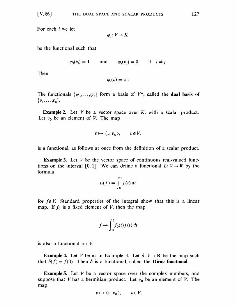
[V, §6] THE DUAL SPACE AND SCALAR PRODUCTS 127
For each i we let
be the functional such that
and if i =1= j.
Then
The functionals {qJ 1, ... ,qJn} form a basis of V*, called the dual basis of {V1' ... ,vn}·
Example 2. Let V be a vector space over K, with a scalar product. Let Vo be an element of V. The map
is a functional, as follows at once from the definition of a scalar product.
Example 3. Let V be the vector space of continuous real-valued functions on the interval [0, 1]. We can define a functional L: V -+ R by the formula
L(f) = ff(t) dt
for fE V. Standard properties of the integral show that this is a linear map. If fo is a fixed element of V, then the map
is also a functional on V.
Example 4. Let V be as in Example 3. Let b: V -+ R be the map such that b(f) = f(O). Then b is a functional, called the Dirac functional.
Example 5. Let V be a vector space over the complex numbers, and suppose that V has a hermitian product. Let Vo be an element of V. The map
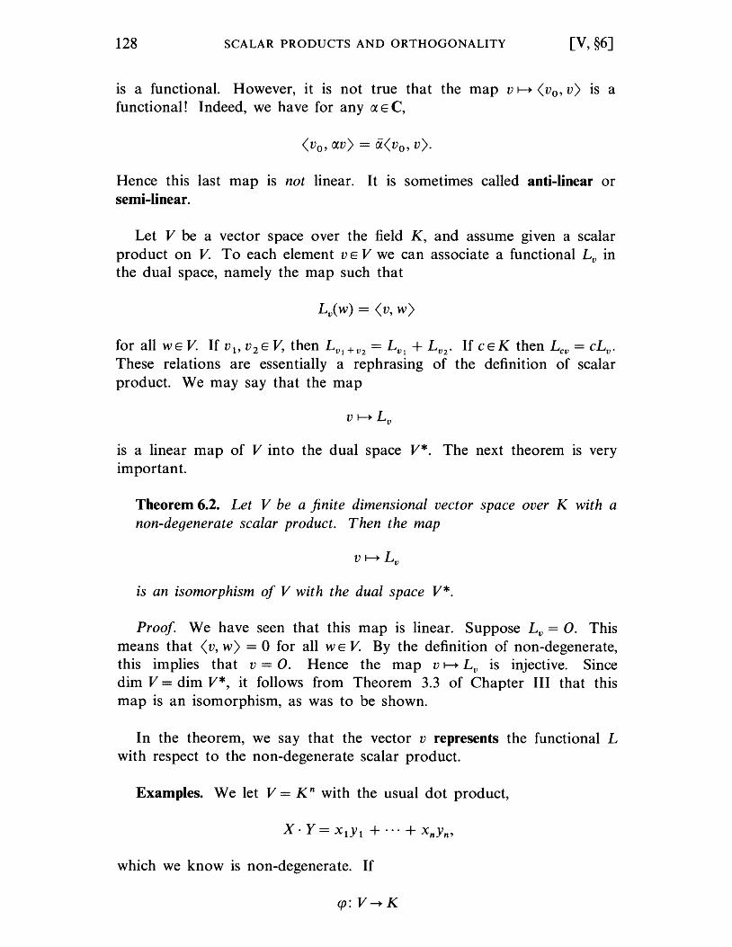
128 SCALAR PRODUCTS AND ORTHOGONALITY [V, §6]
is a functional. However, it is not true that the map v ~ <vo, v) is a functional! Indeed, we have for any C( E C,
Hence this last map IS not linear. It is sometimes called anti-linear or semi-linear.
Let V be a vector space over the field K, and assume given a scalar product on V. To each element v E V we can associate a functional Lv in the dual space, namely the map such that
for all WE V. If Vl' V 2 E V, then Lv! + V2 = Lv! + L v2 . If c E K then Lev = cLv. These relations are essentially a rephrasing of the definition of scalar product. We may say that the map
is a linear map of V into the dual space V*. The next theorem IS very important.
Theorem 6.2. Let V be a finite dimensional vector space over K with a non-degenerate scalar product. Then the map
is an isomorphism of V with the dual space V*.
Proof. We have seen that this map is linear. Suppose Lv = O. This means that <v, w) = 0 for all WE V. By the definition of non-degenerate, this implies that v = O. Hence the map v ~ Lv is injective. Since dim V = dim V*, it follows from Theorem 3.3 of Chapter III that this map is an isomorphism, as was to be shown.
In the theorem, we say that the vector v represents the functional L with respect to the non-degenerate scalar product.
Examples. We let V = K n with the usual dot product,
which we know is non-degenerate. If
qJ:V-+K
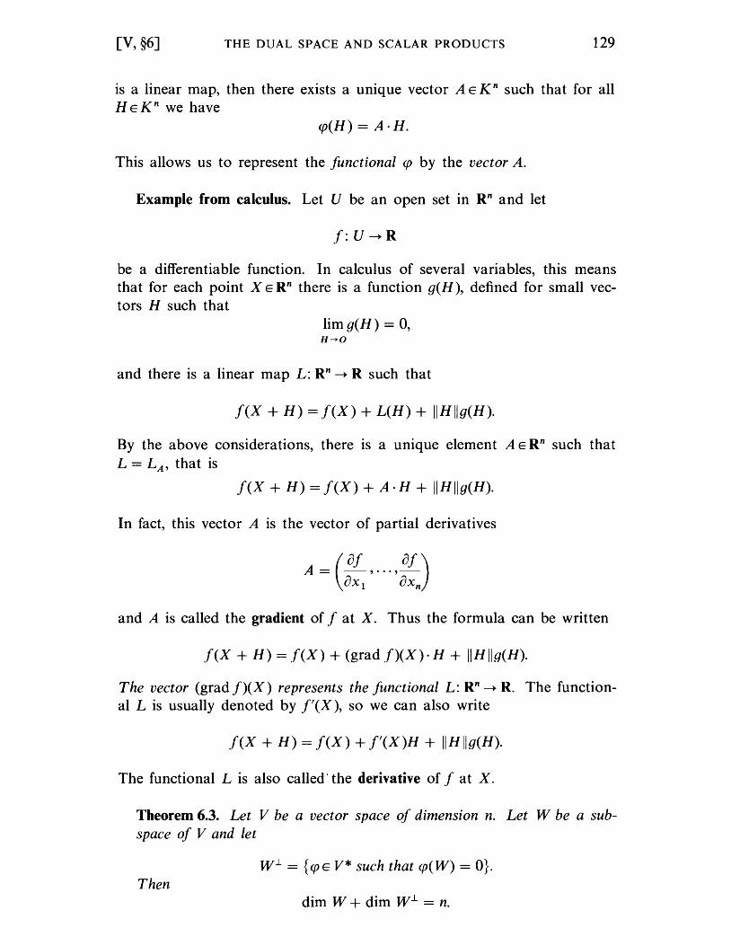
[V, §6] THE DUAL SPACE AND SCALAR PRODUCTS 129
is a linear map, then there exists a unique vector A E K n such that for all HEKn we have
qJ(H) = A·H.
This allows us to represent the functional qJ by the vector A.
Example from calculus. Let U be an open set in Rn and let
f: U -+ R
be a differentiable function. In calculus of several variables, this means that for each point X E Rn there is a function g(H), defined for small vectors H such that
lim g(H) = 0, H-+O
and there is a linear map L: Rn -+ R such that
f(X + H) = f(X) + L(H) + IIHllg(H).
By the above considerations, there is a unique element A E Rn such that L = LA' that is
f(X + H) =f(X) + A·H + IIHllg(H).
In fact, this vector A is the vector of partial derivatives
A = (Of , ... , Of) ox! OXn
and A is called the gradient of f at X. Thus the formula can be written
f(X + H) =f(X) + (gradf)(X)·H + IIHllg(H).
The vector (grad f)(X) represents the functional L: Rn -+ R. The functional L is usually denoted by f'(X), so we can also write
f(X + H) = f(X) + f'(X)H + IIHllg(H).
The functional L is also called' the derivative of f at X.
Theorem 6.3. Let V be a vector space of dimension n. Let W be a subspace of V and let
W1. = {qJE V* such that qJ(W) = O}. Then
dim W + dim W 1. = n.
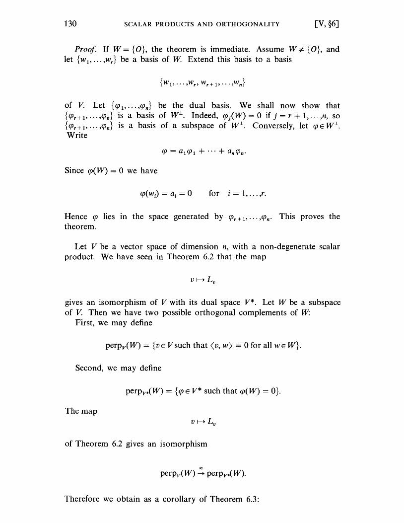
130 SCALAR PRODUCTS AND ORTHOGONALITY [V, §6]
Proof. If W = {O}, the theorem is immediate. Assume W i= {O}, and let {W l' ... ,W r} be a basis of W Extend this basis to a basis
of V. Let {qJ1' ... ,qJn} be the dual basis. We shall now show that {qJr+ 1'··· ,qJn} is a basis of W-L. Indeed, qJj(W) = 0 if j = r + 1, ... ,n, so {qJr+ l' ... ,qJn} is a basis of a subspace of W-L. Conversely, let qJ E W-L. Write
Since qJ(W) = 0 we have
for i = 1, ... ,r.
Hence qJ lies In the space generated by qJr+ 1' ... ,qJn. This proves the theorem.
Let V be a vector space of dimension n, with a non-degenerate scalar product. We have seen in Theorem 6.2 that the map
gives an isomorphism of V with its dual space V*. Let W be a subspace of V. Then we have two possible orthogonal complements of W:
First, we may define
perpv(W) = {VE V such that <v, w) = 0 for all WE w}.
Second, we may define
perpv*(W) = {qJE V* such that qJ(W) = O}.
The map
of Theorem 6.2 gives an isomorphism
Therefore we obtain as a corollary of Theorem 6.3:
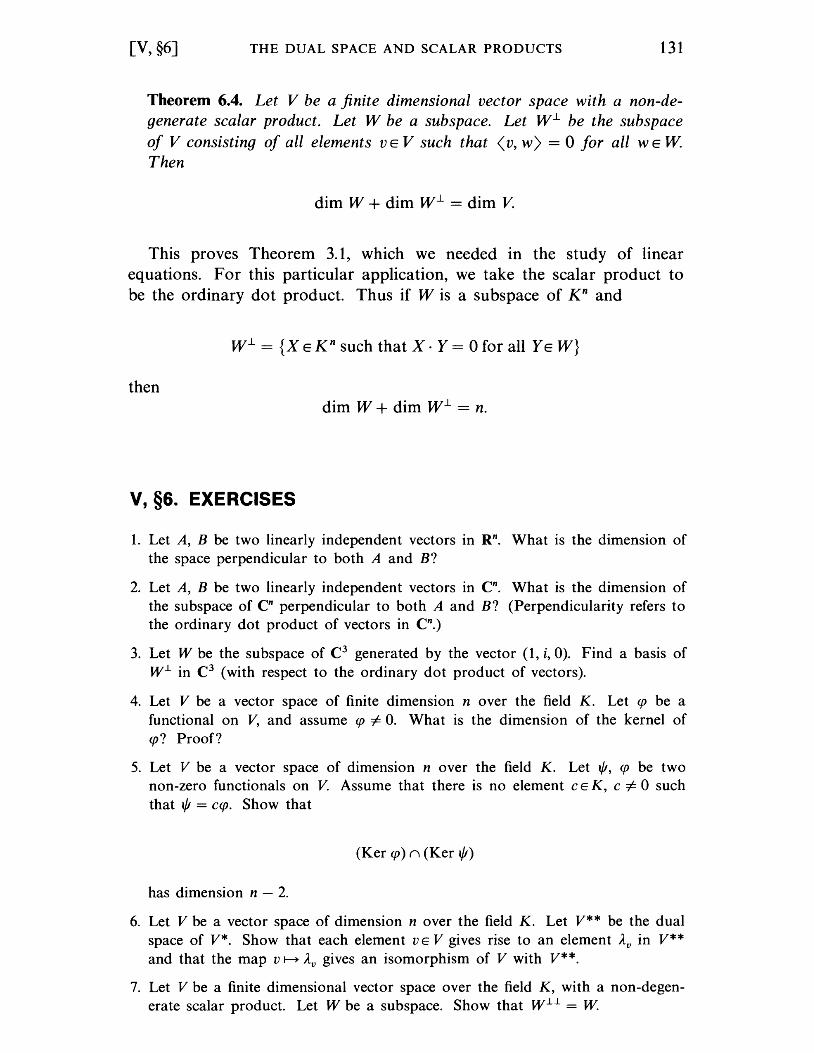
[V, §6] THE DUAL SPACE AND SCALAR PRODUCTS 131
Theorem 6.4. Let V be a finite dimensional vector space with a non-degenerate scalar product. Let W be a subspace. Let W1- be the subspace of V consisting of all elements v E V such that < v, w> = 0 for all WE W Then
dim W + dim W1- = dim V.
This proves Theorem 3.1, which we needed in the study of linear equations. For this particular application, we take the scalar product to be the ordinary dot product. Thus if W is a subspace of K n and
W1- = {X EK n such that X· Y = 0 for all YE W}
then dim W + dim W 1- = n.
V, §6. EXERCISES
1. Let A, B be two linearly independent vectors in Rn. What is the dimension of the space perpendicular to both A and B?
2. Let A, B be two linearly independent vectors in en. What is the dimension of the subspace of en perpendicular to both A and B? (Perpendicularity refers to the ordinary dot product of vectors in en.)
3. Let W be the subspace of e3 generated by the vector (1, i, 0). Find a basis of W1. in e3 (with respect to the ordinary dot product of vectors).
4. Let V be a vector space of finite dimension n over the field K. Let qJ be a functional on V, and assume qJ #- o. What is the dimension of the kernel of qJ? Proof?
5. Let V be a vector space of dimension n over the field K. Let 1/1, qJ be two non-zero functionals on V. Assume that there is no element C E K, c#-O such that t/I = CqJ. Show that
(Ker qJ) n (Ker t/I)
has dimension n - 2.
6. Let V be a vector space of dimension n over the field K. Let V** be the dual space of V*. Show that each element v E V gives rise to an element Av in V** and that the map v 1---+ Av gives an isomorphism of V with V**.
7. Let V be a finite dimensional vector space over the field K, with a non-degenerate scalar product. Let W be a subspace. Show that W 1.1. = W
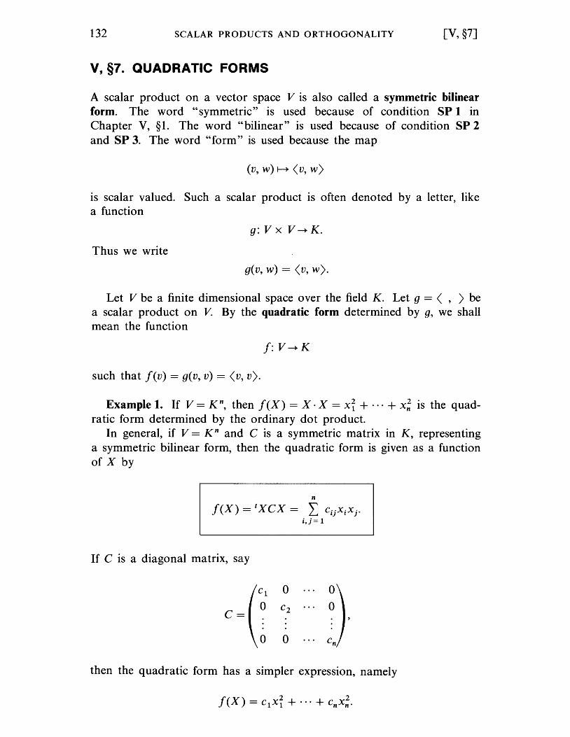
132 SCALAR PRODUCTS AND ORTHOGONALITY [V, §7]
V, §7. QUADRATIC FORMS
A scalar product on a vector space V is also called a symmetric bilinear form. The word "symmetric" is used because of condition SP 1 in Chapter V, §1. The word "bilinear" is used because of condition SP 2 and SP 3. The word "form" is used because the map
(v, w) ~ <v, w)
is scalar valued. Such a scalar product is often denoted by a letter, like a function
g: V x V --+ K.
Thus we write
g(v, w) = <v, w).
Let V be a finite dimensional space over the field K. Let g = < , ) be a scalar product on V. By the quadratic form determined by g, we shall mean the function
f: V --+ K
such that f(v) = g(v, v) = <v, v).
Example 1. If V = K n, then f(X) = X· X = xi + ... + x; is the quad
ratic form determined by the ordinary dot product. In general, if V = K n and C is a symmetric matrix in K, representing
a symmetric bilinear form, then the quadratic form is given as a function of X by
n
f(X) = txcx = L cijxixj •
i,j= 1
If C is a diagonal matrix, say
C1 0 0
C= 0 C2 0
0 0 Cn
then the quadratic form has a simpler expression, namely
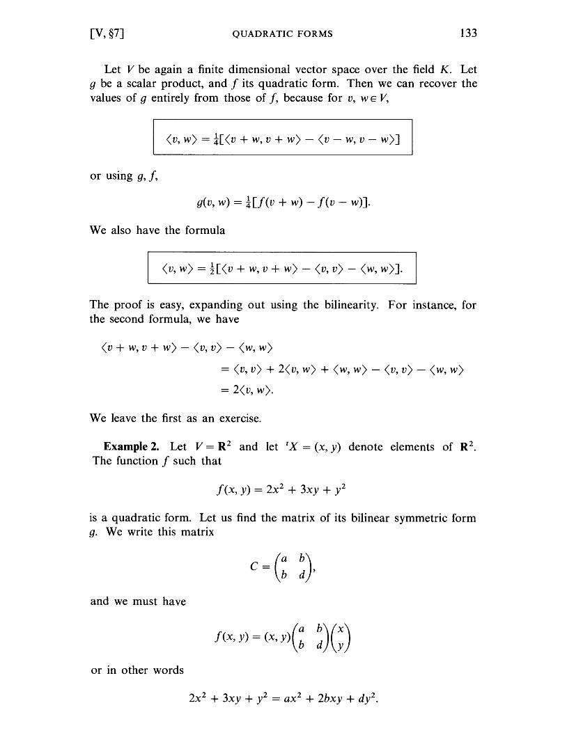
[V, §7] QUADRATIC FORMS 133
Let V be again a finite dimensional vector space over the field K. Let g be a scalar product, and f its quadratic form. Then we can recover the values of g entirely from those of f, because for v, WE V,
<v, W) = i[<v + w, v + W) - <v - w, v - W)]
or using g, f,
g(v, w) = i[f(v + w) - f(v - w)].
We also have the formula
<v, w) = t[<v + w,v + w) - <v, v) - <w, w)].
The proof is easy, expanding out using the bilinearity. For instance, for the second formula, we have
<v + w, v + w) - <v, v) - <w, w)
= <v, v) + 2<v, w) + <w, w) - <v, v) - <w, w)
= 2<v, w).
We leave the first as an exercise.
Example 2. Let V = R2 and let tx = (x, y) denote elements of R2. The function f such that
f(x, y) = 2X2 + 3xy + y2
is a quadratic form. Let us find the matrix of its bilinear symmetric form g. We write this matrix
and we must have
!(X,y)=(X,y)(: ~)G) or in other words
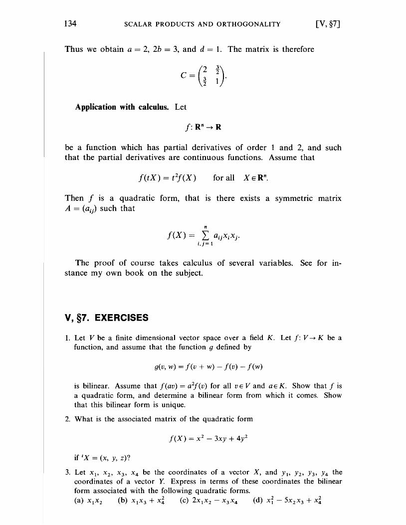
134 SCALAR PRODUCTS AND ORTHOGONALITY [V, §7]
Thus we obtain a = 2, 2b = 3, and d = 1. The matrix is therefore
(2 ~)
C = ~ :.
Application with calculus. Let
f: R n --+ R
be a function which has partial derivatives of order 1 and 2, and such that the partial derivatives are continuous functions. Assume that
for all X ERn.
Then f is a quadratic form, that is there exists a symmetric matrix A = (aij) such that
n
f(X) = L aijxixj . i,j= 1
The proof of course takes calculus of several variables. See for Instance my own book on the subject.
V, §7. EXERCISES
1. Let V be a finite dimensional vector space over a field K. Let f: V --. K be a function, and assume that the function 9 defined by
g(v, w) = f(v + w) - f(v) - f(w)
is bilinear. Assume that f(av) = a2f(v) for all v E V and a E K. Show that f is a quadratic form, and determine a bilinear form from which it comes. Show that this bilinear form is unique.
2. What is the associated matrix of the quadratic form
f(X) = x 2 - 3xy + 4y2
if tx = (x, y, z)?
3. Let Xl' x 2 , x3' X4 be the coordinates of a vector X, and Yl' Y2' Y3' Y4 the coordinates of a vector Y. Express in terms of these coordinates the bilinear form associated with the following quadratic forms. (a) X l X 2 (b) X l X 3 + x~ (c) 2X l X 2 - X 3 X 4 (d) xi - 5X2 X 3 + x~
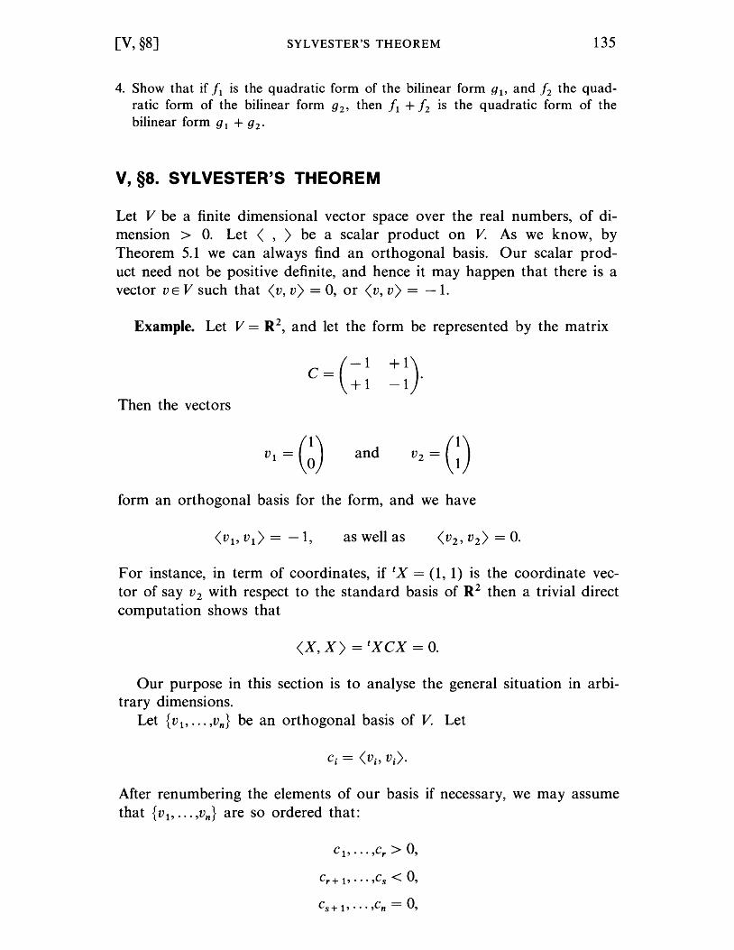
[V, §8] SYLVESTER'S THEOREM 135
4. Show that if 11 is the quadratic form of the bilinear form g1' and 12 the quadratic form of the bilinear form g 2' then 11 + 12 is the quadratic form of the bilinear form g 1 + g 2·
V, §8. SYLVESTER'S THEOREM
Let V be a finite dimensional vector space over the real numbers, of dimension > O. Let < , ) be a scalar product on V. As we know, by Theorem 5.1 we can always find an orthogonal basis. Our scalar product need not be positive definite, and hence it may happen that there is a vector vEVsuch that <v,v) =0, or <v,v) =-1.
Example. Let V = R2, and let the form be represented by the matrix
(-1 c= +1
+1). -1
Then the vectors
and
form an orthogonal basis for the form, and we have
as well as
For instance, in term of coordinates, if tx = (1, 1) is the coordinate vector of say V 2 with respect to the standard basis of R2 then a trivial direct computation shows that
<x, X) = txcx = O.
Our purpose in this section is to analyse the general situation in arbitrary dimensions.
Let {v l , ... ,vn } be an orthogonal basis of V. Let
After renumbering the elements of our basis if necessary, we may assume that {v l , ... ,vn } are so ordered that:
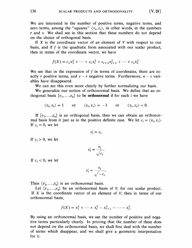
136 SCALAR PRODUCTS AND ORTHOGONALITY [V, §8]
We are interested in the number of positive terms, negative terms, and zero terms, among the "squares" <Vi,Vi), in other words, in the numbers rand s. We shall see in this section that these numbers do not depend on the choice of orthogonal basis.
If X is the coordinate vector of an element of V with respect to our basis, and if f is the quadratic form associated with our scalar product, then in terms of the coordinate vector, we have
We see that in the expression of f in terms of coordinates, there are exactly r positive terms, and s - r negative terms. Furthermore, n - s variables have disappeared.
We can see this even more clearly by further normalizing our basis. We generalize our notion of orthonormal basis. We define that an or
thogonal basis {v l , ... ,vn } to be orthonormal if for each i we have
or or
If {v l , ... ,vn } is an orthogonal basis, then we can obtain an orthonormal basis from it just as in the positive definite case. We let Ci = <Vi' Vi).
If Ci = 0, we let
If Ci > 0, we let
If Ci < 0, we let
Then {V'l , ... ,v~} is an orthonormal basis. Let {v l , ... ,vn} be an orthonormal basis of V, for our scalar product.
If X is the coordinate vector of an element of V, then in terms of our orthonormal basis,
f(X) - 2 2 2 2 - Xl + ... + Xr - Xr + l - ... - Xs·
By using an orthonormal basis, we see the number of positive and negative terms particularly clearly. In proving that the number of these does not depend on the orthonormal basis, we shall first deal with the number of terms which disappear, and we shall give a geometric interpretation for it.
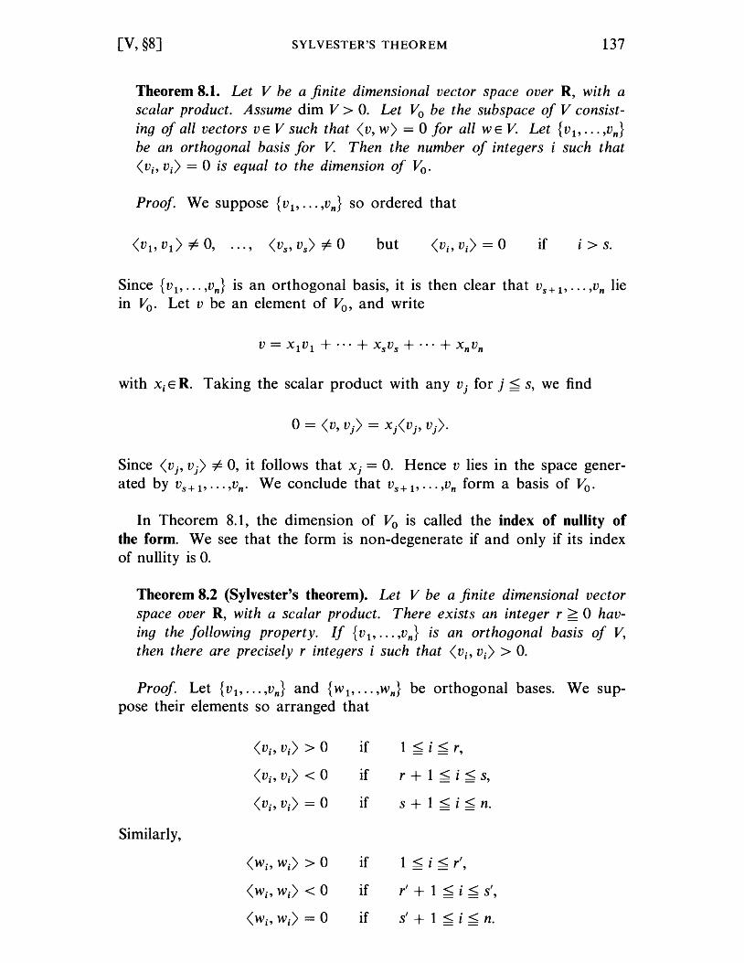
[V, §8] SYLVESTER'S THEOREM 137
Theorem 8.1. Let V be a finite dimensional vector space over R, with a scalar product. Assume dim V > O. Let Vo be the subspace of V consisting of all vectors v E V such that <v, w) = 0 for all WE V. Let {v l' ... ,vn }
be an orthogonal basis for V. Then the number of integers i such that < Vi' Vi) = 0 is equal to the dimension of Vo.
Proof. We suppose {v 1, ••• ,vn } so ordered that
but if i > s.
Since {v 1, ••• ,vn } is an orthogonal basis, it is then clear that vs + l' ... ,Vn lie in Vo. Let v be an element of Vo, and write
with Xi E R. Taking the scalar product with any v j for j < s, we find
Since <Vj' Vj) ;;/= 0, it follows that Xj = o. Hence v lies in the space generated by Vs + 1 , ••• ,Vn • We conclude that VS + 1' ••• 'Vn form a basis of Vo.
In Theorem 8.1, the dimension of Vo is called the index of nullity of the form. We see that the form is non-degenerate if and only if its index of nullity is o.
Theorem 8.2 (Sylvester's theorem). Let V be a finite dimensional vector space over R, with a scalar product. There exists an integer r > 0 having the following property. If {v 1, ••• ,vn } is an orthogonal basis of V, then there are precisely r integers i such that <Vi' Vi) > O.
Proof. Let {v 1, ••• ,vn} and {w 1, ••• ,wn} be orthogonal bases. We suppose their elements so arranged that
Similarly,
<Vi' Vi) > 0
<Vi'Vi) < 0
<Vi'Vi) = 0
<Wi' Wi) > 0
<Wi' Wi) < 0
<Wi' Wi) = 0
if
if
if
if
if
if
1 < i < r,
r + 1 < i < s,
s + 1 < i < n.
1 < i < r',
r' + 1 < i < s',
s' + 1 < i < n.
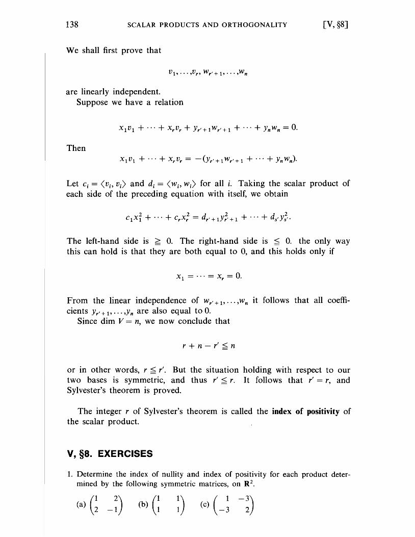
138 SCALAR PRODUCTS AND ORTHOGONALITY [V, §8]
We shall first prove that
are linearly independent. Suppose we have a relation
Then X 1 V1 + ... + XrVr = -(Yr'+lWr'+l + ... + YnWn)·
Let C i = <Vi' Vi) and di = <Wi' Wi) for all i. Taking the scalar product of each side of the preceding equation with itself, we obtain
The left-hand side is > O. The right-hand side is < O. the only way this can hold is that they are both equal to 0, and this holds only if
From the linear independence of W r, + 1' ... ,wn it follows that all coefficients Yr' + l' ... ,Yn are also equal to o.
Since dim V = n, we now conclude that
r+n-r'<n
or in other words, r < r'. But the situation holding with respect to our two bases is symmetric, and thus r' < r. It follows that r' = r, and Sylvester's theorem is proved.
The integer r of Sylvester's theorem is called the index of positivity of the scalar product.
V, §8. EXERCISES
1. Determine the index of nullity and index of positivity for each product determined by the following symmetric matrices, on R 2 •
(b) G ~)
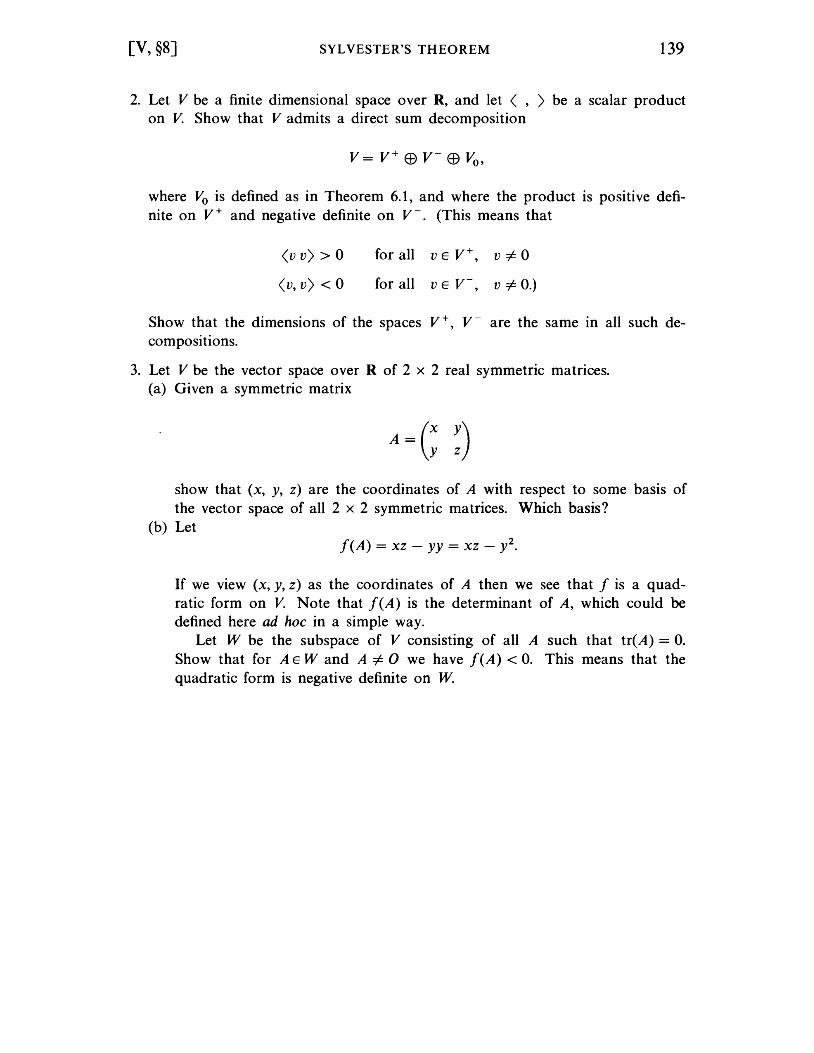
[V, §8] SYLVESTER'S THEOREM 139
2. Let V be a finite dimensional space over R, and let ( , ) be a scalar product on V. Show that V admits a direct sum decomposition
where Vo is defined as in Theorem 6.1, and where the product is positive definite on V + and negative definite on V -. (This means that
(v v) > 0
(v, v) < 0
for all v E V+, v#-o
for all v E V-, v #- 0.)
Show that the dimensions of the spaces V +, V - are the same in all such decom positions.
3. Let V be the vector space over R of 2 x 2 real symmetric matrices. (a) Given a symmetric matrix
show that (x, y, z) are the coordinates of A with respect to some basis of the vector space of all 2 x 2 symmetric matrices. Which basis?
(b) Let f(A) = xz - yy = xz - y2.
If we view (x, y, z) as the coordinates of A then we see that f is a quadratic form on V. Note that f(A) is the determinant of A, which could be defined here ad hoc in a simple way.
Let W be the subspace of V consisting of all A such that tr(A) = O. Show that for A E Wand A#-O we have f(A) < o. This means that the quadratic form is negative definite on W.
CHAPTER VI
Determ i nants
We have worked with vectors for some time, and we have often felt the need of a method to determine when vectors are linearly independent. Up to now, the only method available to us was to solve a system of linear equations by the elimination method. In this chapter, we shall exhibit a very efficient computational method to solve linear equations, and determine when vectors are linearly independent.
The cases of 2 x 2 and 3 x 3 determinants will be carried out separately in full, because the general case of n x n determinants involves notation which adds to the difficulties of understanding determinants. In a first reading, we suggest omitting the proofs in the general case.
VI, §1. DETERMINANTS OF ORDER 2
Before stating the general properties of an arbitrary determinant, we shall consider a special case.
Let
be a 2 x 2 matrix in a field K. We define its determinant to be ad - be. Thus the determinant is an element of K. We denote it by
a b = ad - be.
e d
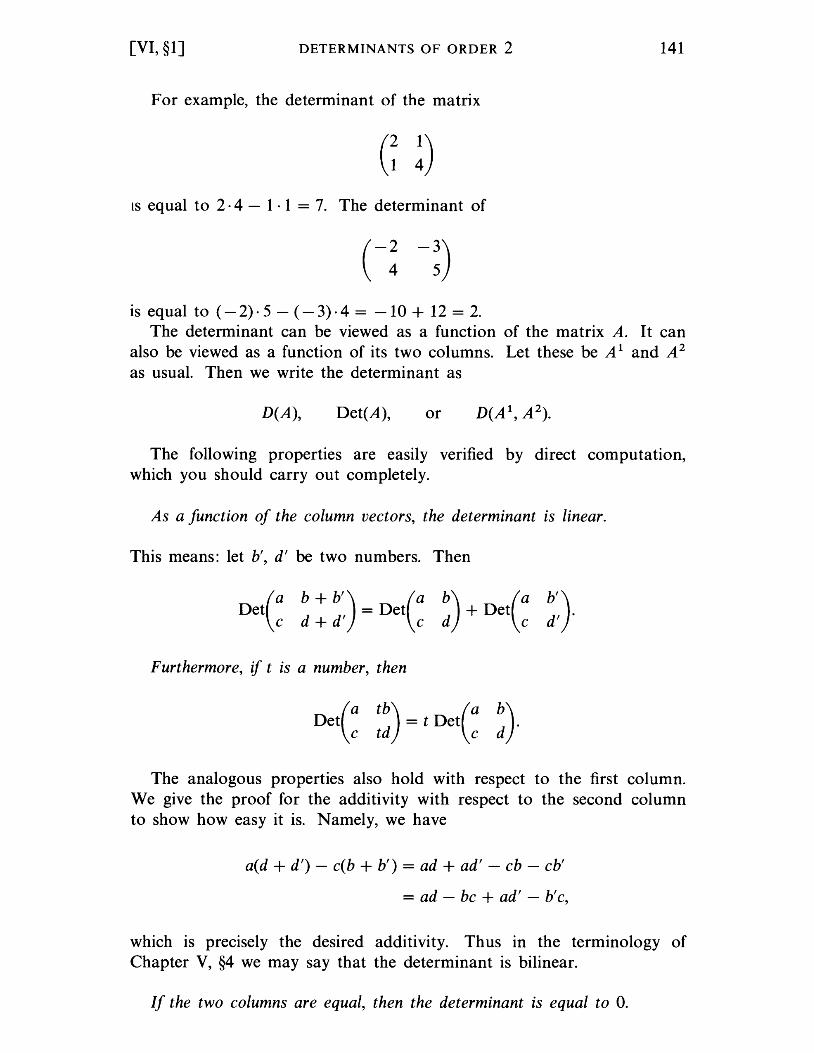
[VI, §1] DETERMINANTS OF ORDER 2 141
For example, the determinant of the matrix
lS equal to 2·4 - 1 . 1 = 7. The determinant of
is equal to (- 2)·5 - ( - 3)·4 = -10 + 12 = 2. The determinant can be viewed as a function of the matrix A. It can
also be viewed as a function of its two columns. Let these be A 1 and A 2
as usual. Then we write the determinant as
D(A), Det(A), or
The following properties are easily verified by direct computation, which you should carry out completely.
As a function of the column vectors, the determinant is linear.
This means: let b', d' be two numbers. Then
Furthermore, if t is a number, then
Det(a tb) = t Det(a b) c td cd·
The analogous properties also hold with respect to the first column. We give the proof for the additivity with respect to the second column to show how easy it is. Namely, we have
a(d + d') - c(b + b') = ad + ad' - cb - cb'
= ad - bc + ad' - b' c,
which is precisely the desired additivity. Thus in the terminology of Chapter V, §4 we may say that the determinant is bilinear.
If the two columns are equal, then the determinant is equal to O.
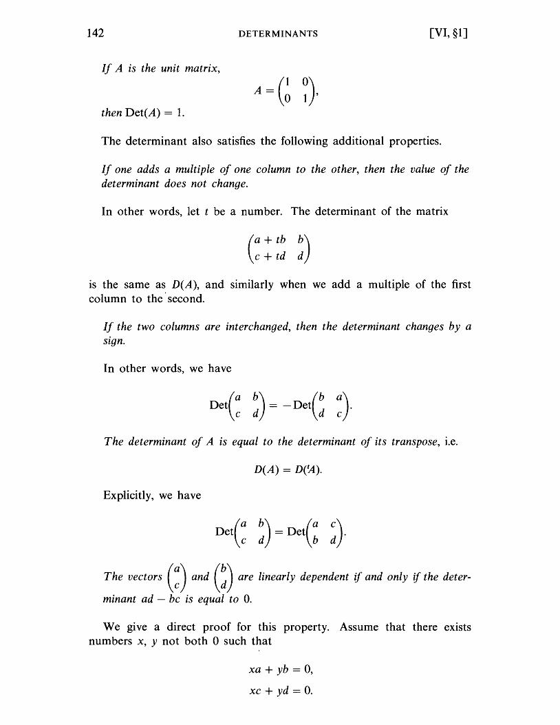
142 DETERMINANTS [VI, §1]
If A is the unit matrix,
then Det(A) = 1.
The determinant also satisfies the following additional properties.
If one adds a multiple of one column to the other, then the value of the determinant does not change.
In other words, let t be a number. The determinant of the matrix
(a + tb b) c + td d
is the same as D(A), and similarly when we add a multiple of the first column to the' second.
If the two columns are interchanged, then the determinant changes by a sign.
In other words, we have
The determinant of A is equal to the determinant of its transpose, i.e.
D(A) = D(~).
Explicitly, we have
The vectors (:) and (~) are linearly dependent if and only if the deter
minant ad - bc is equal to O.
We give a direct proof for this property. Assume that there exists numbers x, y not both 0 such that
xa + yb = 0,
xc + yd = O.
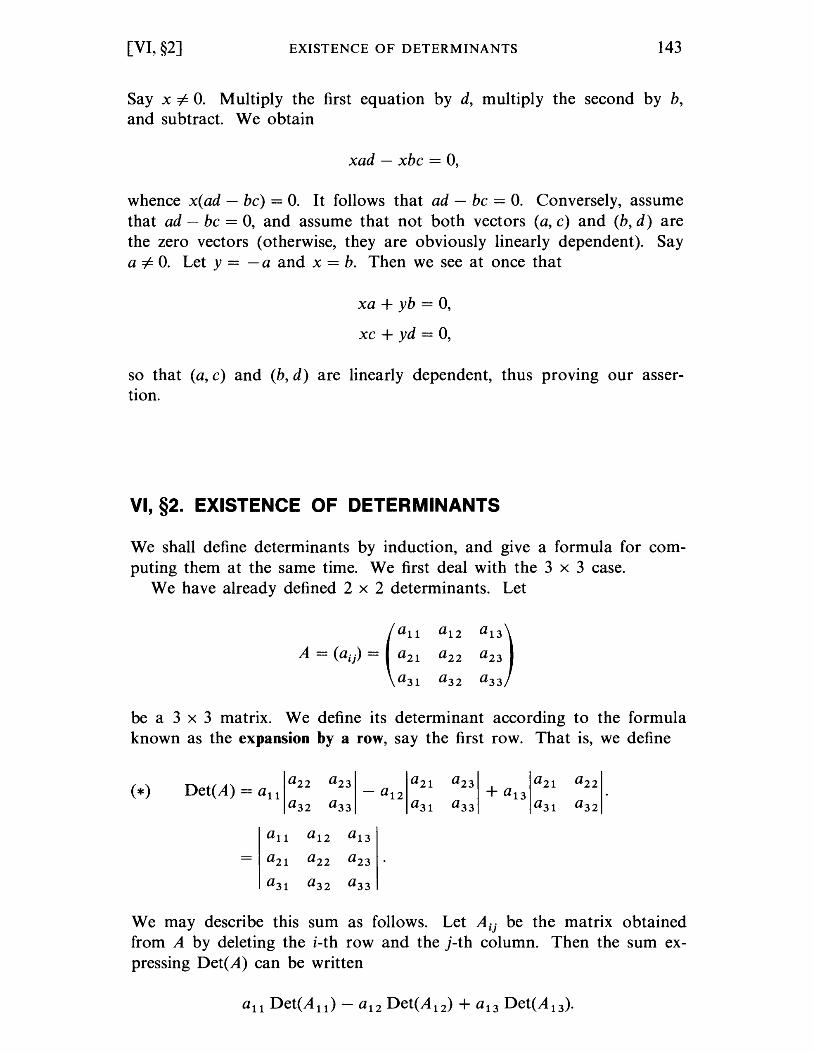
[VI, §2] EXISTENCE OF DETERMINANTS 143
Say x =1= O. Multiply the first equation by d, multiply the second by b, and subtract. We obtain
xad - xbe = 0,
whence x(ad - be) = O. It follows that ad - be = O. Conversely, assume that ad - be = 0, and assume that not both vectors (a, e) and (b, d) are the zero vectors (otherwise, they are obviously linearly dependent). Say a =1= O. Let y = - a and x = b. Then we see at once that
xa + yb = 0,
xe + yd = 0,
so that (a, e) and (b, d) are linearly dependent, thus provIng our assertion.
VI, §2. EXISTENCE OF DETERMINANTS
We shall define determinants by induction, and give a formula for computing them at the same time. We first deal with the 3 x 3 case.
We have already defined 2 x 2 determinants. Let
al2 a l3 ) a22 a23
a32 a33
be a 3 x 3 matrix. We define its determinant according to the formula known as the expansion by a row, say the first row. That is, we define
(*) Det(A) = all a22 a23 a2l a23 + al 3
a2l a22 - a l2 a32 a33 a3l a33 a3l a32
all al2 al 3 a2l a22 a23 a3l a32 a33
We may describe this sum as follows. Let Aij be the matrix obtained from A by deleting the i-th row and the j-th column. Then the sum expressing Det(A) can be written
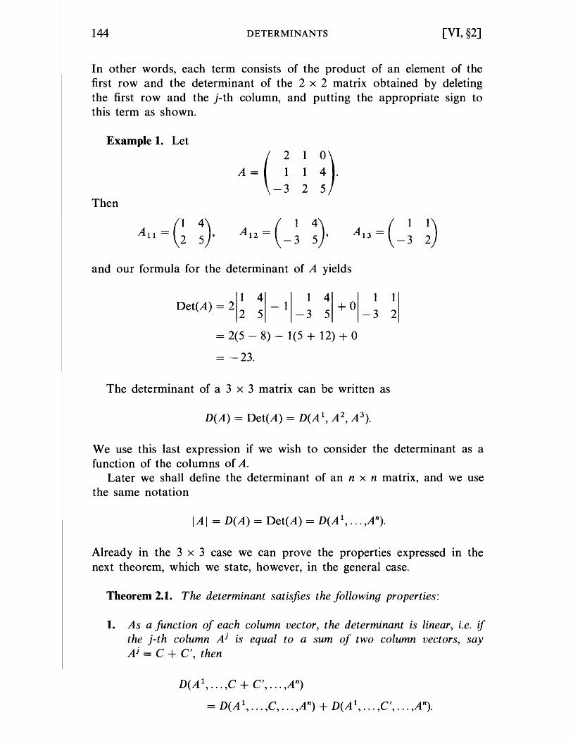
144 DETERMINANTS [VI, §2]
In other words, each term consists of the product of an element of the first row and the determinant of the 2 x 2 matrix obtained by deleting the first row and the j-th column, and putting the appropriate sign to this term as shown.
Example 1. Let
A = ( ~ ! ~). -3 2 5
Then
and our formula for the determinant of A yields
1 4 1 4 1 1 Det( A) = 2 2 5 - 1 _ 3 5 + 0 - 3 2
= 2(5 - 8) - 1(5 + 12) + 0
= -23.
The determinant of a 3 x 3 matrix can be written as
We use this last expression if we wish to consider the determinant as a function of the columns of A.
Later we shall define the determinant of an n x n matrix, and we use the same notation
IAI = D(A) = Det(A) = D(Al, ... ,An).
Already in the 3 x 3 case we can prove the properties expressed in the next theorem, which we state, however, in the general case.
Theorem 2.1. The determinant satisfies the following properties:
1. As a function of each column vector, the determinant is linear, i.e. if the j-th column Ai is equal to a sum of two column vectors, say Ai = C + C', then
D(A 1, ... ,C + C', ... ,An)
= D( A 1, ... ,C, ... ,A n) + D( A 1 , ... ,C', ... ,A n).
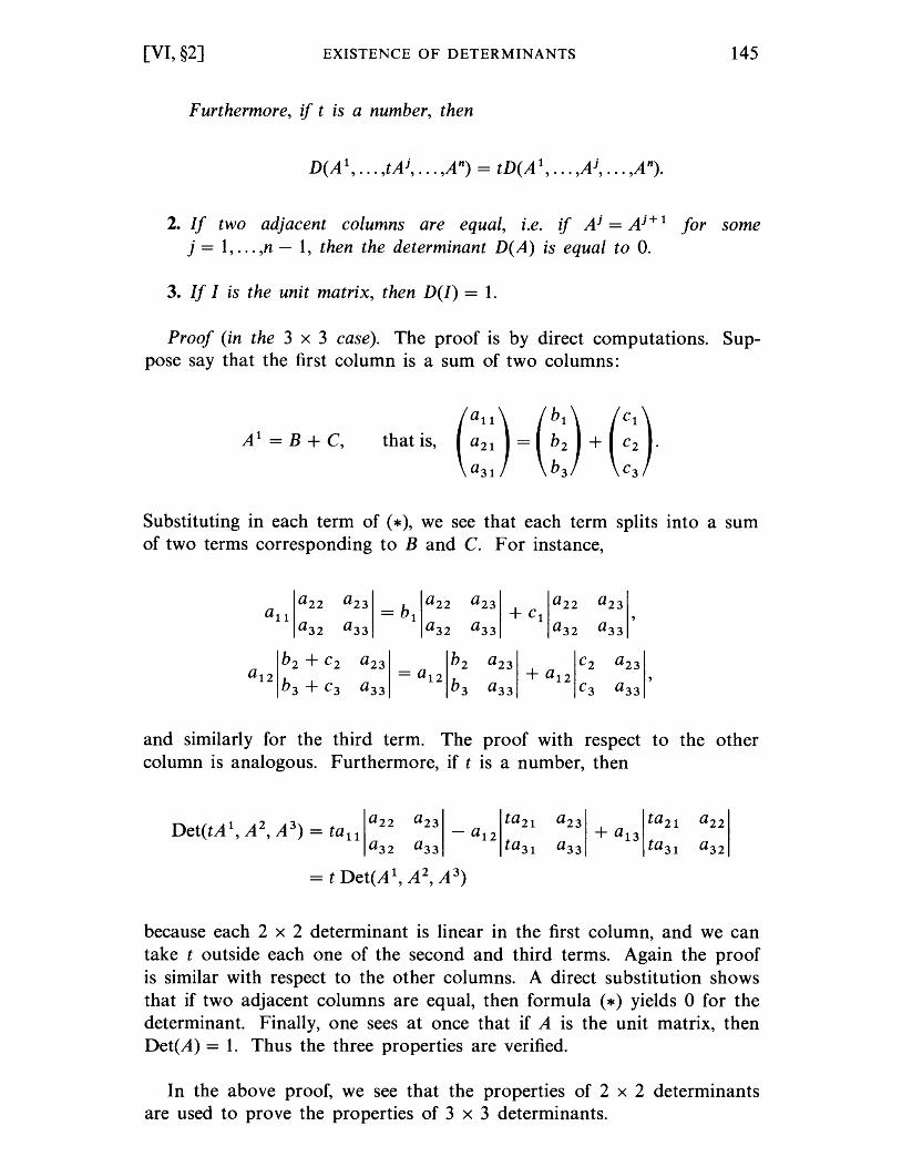
[VI, §2] EXISTENCE OF DETERMINANTS 145
Furthermore, if t is a number, then
D(A 1, ... ,tAi, ... ,An) = tD(A 1, ... ,Ai, ... ,An).
2. If two adjacent columns are equal, i.e. if Ai = Ai+ 1 for some j = 1, ... ,n - 1, then the determinant D( A) is equal to O.
3. If I is the unit matrix, then D(I) = 1.
Proof (in the 3 x 3 case). The proof is by direct computations. Suppose say that the first column is a sum of two columns:
Al = B + C,
Substituting in each term of (*), we see that each term splits into a sum of two terms corresponding to Band C. For instance,
a22 a23 = b l
a22 a23 + C1 a22 a23
all a32 a33 a32 a33 a32 a33
b2 + c2 a23 b2 a23 + a 12
c2 a23 a 12 h3 + c3
= a 12 h3 a33 a33 a33 c3
and similarly for the third term. The proof with respect to the other column is analogous. Furthermore, if t is a number, then
because each 2 x 2 determinant is linear in the first column, and we can take t outside each one of the second and third terms. Again the proof is similar with respect to the other columns. A direct substitution shows that if two adjacent columns are equal, then formula (*) yields 0 for the determinant. Finally, one sees at once that if A is the unit matrix, then Det(A) = 1. Thus the three properties are verified.
In the above proof, we see that the properties of 2 x 2 determinants are used to prove the properties of 3 x 3 determinants.
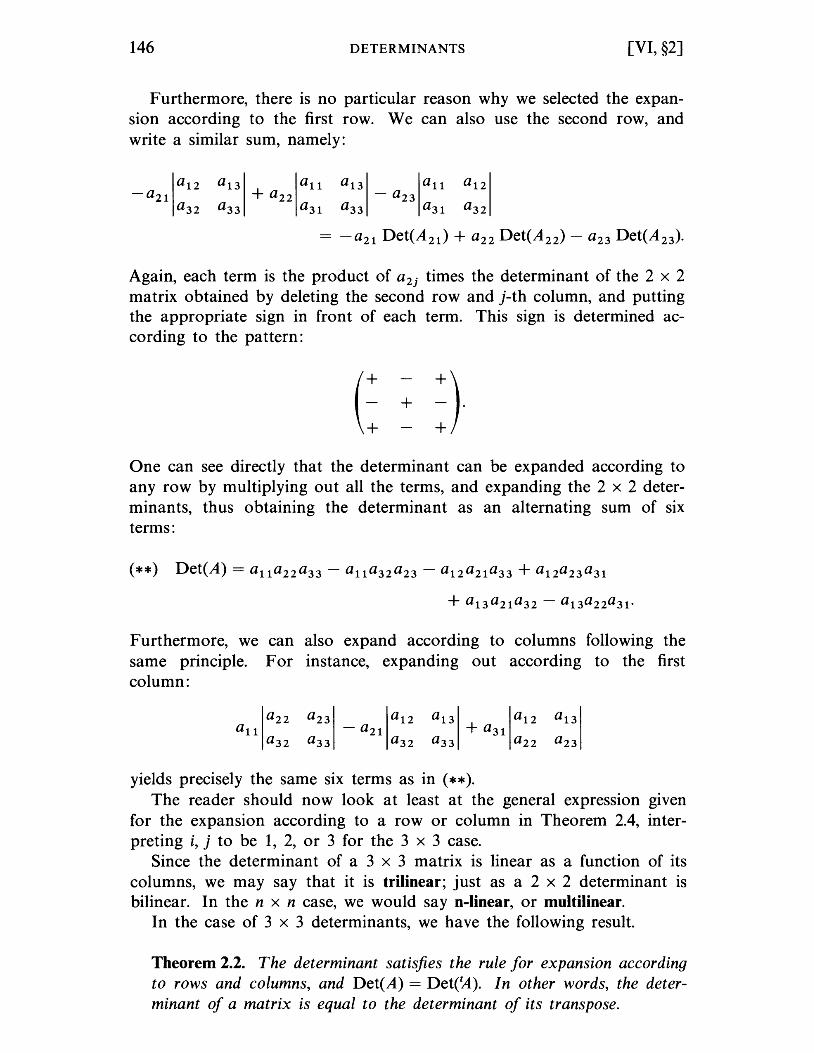
146 DETERMINANTS [VI, §2]
Furthermore, there is no particular reason why we selected the expansion according to the first row. We can also use the second row, and write a similar sum, namely:
Again, each term is the product of a2j times the determinant of the 2 x 2 matrix obtained by deleting the second row and j-th column, and putting the appropriate sign in front of each term. This sign is determined according to the pattern:
One can see directly that the determinant can be expanded according to any row by multiplying out all the terms, and expanding the 2 x 2 determinants, thus obtaining the determinant as an alternating sum of six terms:
Furthermore, we can also expand according to columns following the same principle. For instance, expanding out according to the first column:
yields precisely the same six terms as in (**). The reader should now look at least at the general expression given
for the expansion according to a row or column in Theorem 2.4, interpreting i, j to be 1, 2, or 3 for the 3 x 3 case.
Since the determinant of a 3 x 3 matrix is linear as a function of its columns, we may say that it is trilinear; just as a 2 x 2 determinant IS
bilinear. In the n x n case, we would say n-linear, or multilinear. In the case of 3 x 3 determinants, we have the following result.
Theorem 2.2. The determinant satisfies the rule for expansion according to rows and columns, and Det(A) = Det(~). In other words, the determinant of a matrix is equal to the determinant of its transpose.
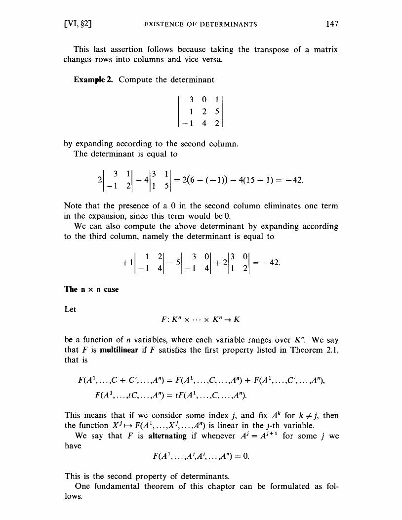
[VI, §2] EXISTENCE OF DETERMINANTS 147
This last assertion follows because taking the transpose of a matrix changes rows into columns and vice versa.
Example 2. Compute the determinant
301
125
-1 4 2
by expanding according to the second column. The determinant is equal to
2 3
-1 1 3
-4 2 1
1 5 =2(6-(-1»)-4(15-1)= -42.
Note that the presence of a 0 in the second column eliminates one term in the expansion, since this term would be O.
We can also compute the above determinant by expanding according to the third column, namely the determinant is equal to
The n x n case
Let
1 + 1 -1
23030 4 - 5 -1 4 + 2 1 2 = -42.
F: K n x ... x K n ~ K
be a function of n variables, where each variable ranges over Kn. We say that F is multilinear if F satisfies the first property listed in Theorem 2.1, that is
F(Al, ... ,C + C', ... ,An) = F(Al, ... ,C, ... ,An) + F(Al, ... ,C', ... ,An),
F(A 1, ... ,tC, ... ,An) = tF(A 1, ... ,C, ... ,An).
This means that if we consider some index j, and fix Ak for k i= j, then the function Xi H F(A 1, ... ,X i, ... ,An) is linear in the j-th variable.
We say that F is alternating if whenever Ai = Ai+ 1 for some j we have
F(A 1, ... ,Ai,Ai, ... ,An) = O.
This is the second property of determinants. One fundamental theorem of this chapter can be formulated as fol
lows.
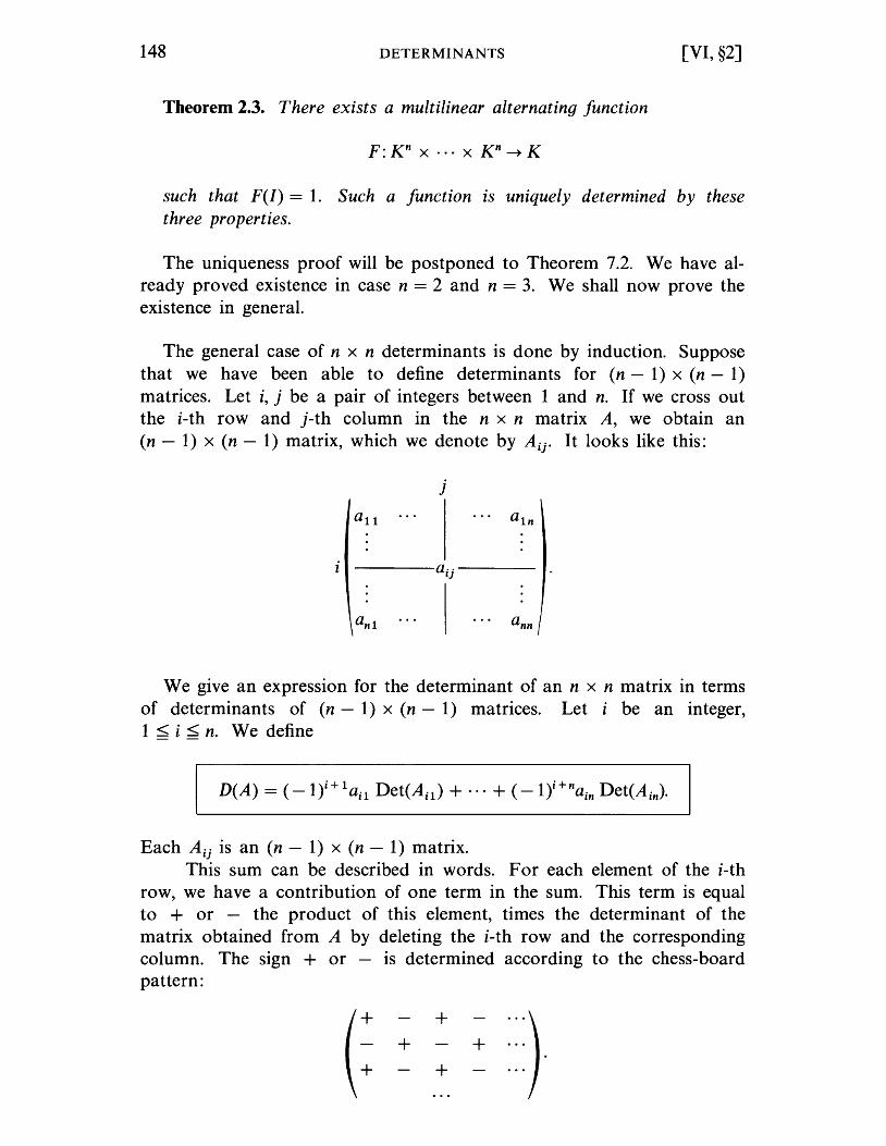
148 DETERMINANTS [VI, §2]
Theorem 2.3. There exists a multilinear alternating function
F:Knx···xKn~K
such that F(J) = 1. Such a function is uniquely determined by these three properties.
The uniqueness proof will be postponed to Theorem 7.2. We have already proved existence in case n = 2 and n = 3. We shall now prove the existence in general.
The general case of n x n determinants is done by induction. Suppose that we have been able to define determinants for (n - 1) x (n - 1) matrices. Let i, j be a pair of integers between 1 and n. If we cross out the i-th row and j-th column in the n x n matrix A, we obtain an (n - 1) x (n - 1) matrix, which we denote by A ij • It looks like this:
j
all
aij
anl
We give an expression for the determinant of an n x n matrix in terms of determinants of (n - 1) x (n - 1) matrices. Let i be an integer, 1 < i < n. We define
Each Aij is an (n - 1) x (n - 1) matrix. This sum can be described in words. For each element of the i-th
row, we have a contribution of one term in the sum. This term is equal to + or - the product of this element, times the determinant of the matrix obtained from A by deleting the i-th row and the corresponding column. The sign + or - is determined according to the chess-board pattern:
+ + ... ) ... + + + +
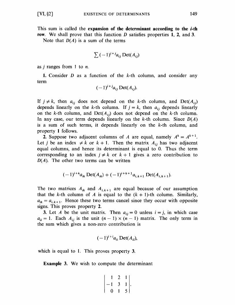
[VI, §2] EXISTENCE OF DETERMINANTS 149
This sum is called the expansion of the determinant according to the i-th row. We shall prove that this function D satisfies properties 1, 2, and 3.
Note that D(A) is a sum of the terms
L (-IY+jaij Det(Aij)
as j ranges from 1 to n.
1. Consider D as a function of the k-th column, and consider any term
If j i= k, then aij does not depend on the k-th column, and Det(Aij) depends linearly on the k-th column. If j = k, then aij depends linearly on the k-th column, and Det(Aij) does not depend on the k-th column. In any case, our term depends linearly on the k-th column. Since D(A) is a sum of such terms, it depends linearly on the k-th column, and property 1 follows.
2. Suppose two adjacent columns of A are equal, namely Ak = A k+ 1. Let j be an index i= k or k + 1. Then the matrix Aij has two adjacent equal columns, and hence its determinant is equal to O. Thus the term corresponding to an index j i= k or k + 1 gives a zero contribution to D(A). The other two terms can be written
i+k i+k+1 (-1) aik Det(Aik) + (-1) ai,k+1 Det(Ai,k+ 1).
The two matrices Aik and Ai,k+ 1 are equal because of our assumption that the k-th column of A is equal to the (k + 1)-th column. Similarly, aik = ai, k + 1· Hence these two terms cancel since they occur with opposite signs. This proves property 2.
3. Let A be the unit matrix. Then aij = 0 unless i = j, in which case aii = 1. Each Aij is the unit (n - 1) x (n - 1) matrix. The only term in the sum which gives a non-zero contribution is
which is equal to 1. This proves property 3.
Example 3. We wish to compute the determinant
121 -1 3 1. 015
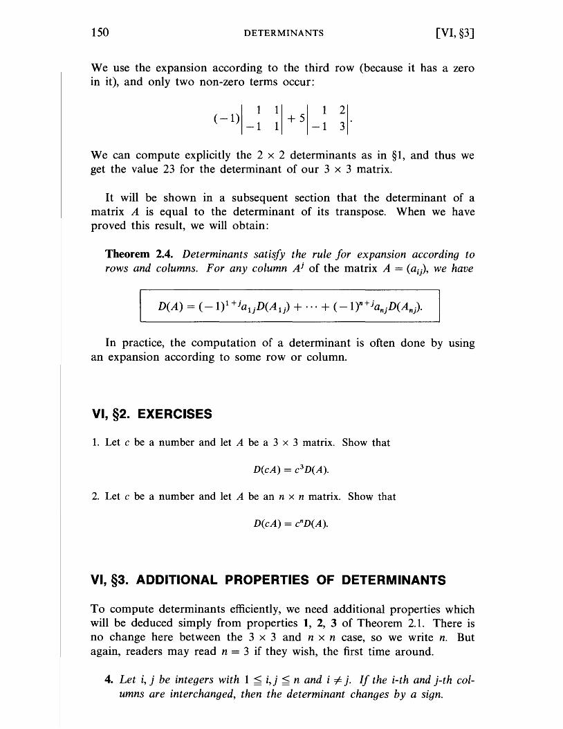
150 DETERMINANTS [VI, §3]
We use the expansion according to the third row (because it has a zero in it), and only two non-zero terms occur:
1 ( -1)
-1 1 1 2 1+ 5 -13.
We can compute explicitly the 2 x 2 determinants as in §1, and thus we get the value 23 for the determinant of our 3 x 3 matrix.
It will be shown in a subsequent section that the determinant of a matrix A is equal to the determinant of its transpose. When we have proved this result, we will obtain:
Theorem 2.4. Determinants satisfy the rule for expansion according to rows and columns. For any column Ai of the matrix A = (aij), we have
In practice, the computation of a determinant is often done by using an expansion according to some row or column.
VI, §2. EXERCISES
1. Let c be a number and let A be a 3 x 3 matrix. Show that
D(cA) = c3D(A).
2. Let c be a number and let A be an n x n matrix. Show that
D(cA) = cnD(A).
VI, §3. ADDITIONAL PROPERTIES OF DETERMINANTS
To compute determinants efficiently, we need additional properties which will be deduced simply from properties 1, 2, 3 of Theorem 2.1. There is no change here between the 3 x 3 and n x n case, so we write n. But again, readers may read n = 3 if they wish, the first time around.
4. Let i, j be integers with 1 < i, j < nand i i= j. If the i-th and j-th columns are interchanged, then the determinant changes by a sign.
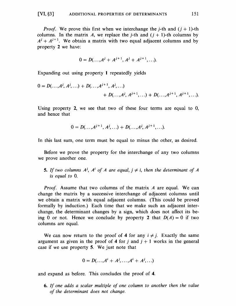
[VI, §3] ADDITIONAL PROPERTIES OF DETERMINANTS 151
Proof. We prove this first when we interchange the j-th and (j + l)-th columns. In the matrix A, we replace the j-th and (j + l)-th columns by Ai + Ai+1. We obtain a matrix with two equal adjacent columns and by property 2 we have:
Expanding out using property 1 repeatedly yields
o = D( ... ,Ai, Ai, ... ) + D( ... ,Ai+ 1, Ai, ... )
. ·+1 ·+1 ·+1 + D( ... ,AJ, AJ , ... ) + D( ... ,AJ , AJ , ... ).
Using property 2, we see that two of these four terms are equal to 0, and hence that
o == D( ... ,Ai+ 1, Ai, ... ) + D( ... ,Ai, Ai+ 1, ... ).
In this last sum, one term must be equal to minus the other, as desired.
Before we prove the property for the interchange of any two columns we prove another one.
5. If two columns Ai, Ai of A are equal, j i= i, then the determinant of A is equal to O.
Proof. Assume that two columns of the matrix A are equal. We can change the matrix by a successive interchange of adjacent columns until we obtain a matrix with equal adjacent columns. (This could be proved formally by induction.) Each time that we make such an adjacent interchange, the determinant changes by a sign, which does not affect its being 0 or not. Hence we conclude by property 2 that D(A) = 0 if two columns are equal.
We can now return to the proof of 4 for any i i= j. Exactly the same argument as given in the proof of 4 for j and j + 1 works in the general case if we use property 5. We just note that
0= D( ... ,Ai + Ai, ... ,Ai + Ai, ... )
and expand as before. This concludes the proof of 4.
6. If one adds a scalar multiple of one column to another then the value of the determinant does not change.
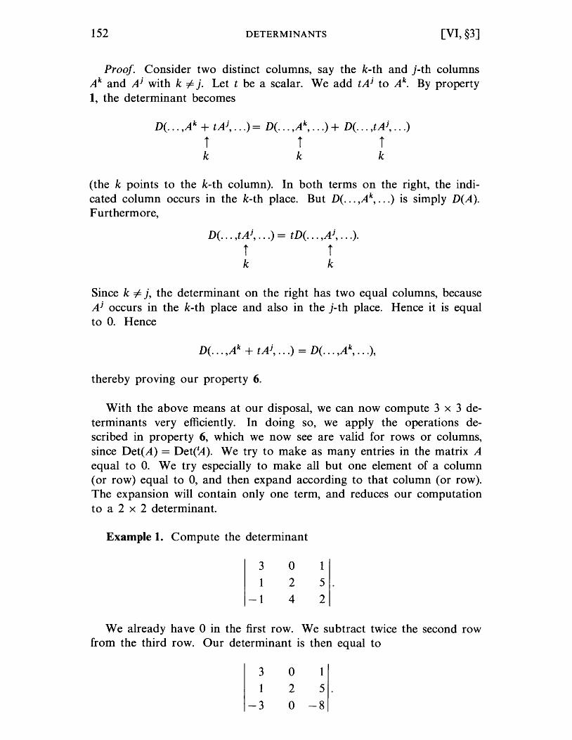
152 DETERMINANTS [VI, §3]
Proof. Consider two distinct columns, say the k-th and j-th columns Ak and Ai with k i= j. Let t be a scalar. We add tAi to Ak. By property 1, the determinant becomes
D( ... ,Ak + tAi, ... ) = D( ... ,Ak, ... ) + D( ... ,tAi, ... )
iii k k k
(the k points to the k-th column). In both terms on the right, the indicated column occurs in the k-th place. But D( ... ,Ak, ... ) is simply D(A). Furthermore,
D( . .. ,tAi, ... ) = tD( ... ,Ai, ... ).
i i k k
Since k i= j, the determinant on the right has two equal columns, because Ai occurs in the k-th place and also in the j-th place. Hence it is equal to O. Hence
D( ... ,Ak + tAi, ... ) = D( ... ,Ak, ... ),
thereby proving our property 6.
With the above means at our disposal, we can now compute 3 x 3 determinants very efficiently. In doing so, we apply the operations described in property 6, which we now see are valid for rows or columns, since Det(A) = Det(~). We try to make as many entries in the matrix A equal to O. We try especially to make all but one element of a column (or row) equal to 0, and then expand according to that column (or row). The expansion will contain only one term, and reduces our computation to a 2 x 2 determinant.
Example 1. Compute the determinant
3
1
-1
o 2 4
1
5 .
2
We already have 0 in the first row. We subtract twice the second row from the third row. Our determinant is then equal to
301
1 25.
-3 0-8
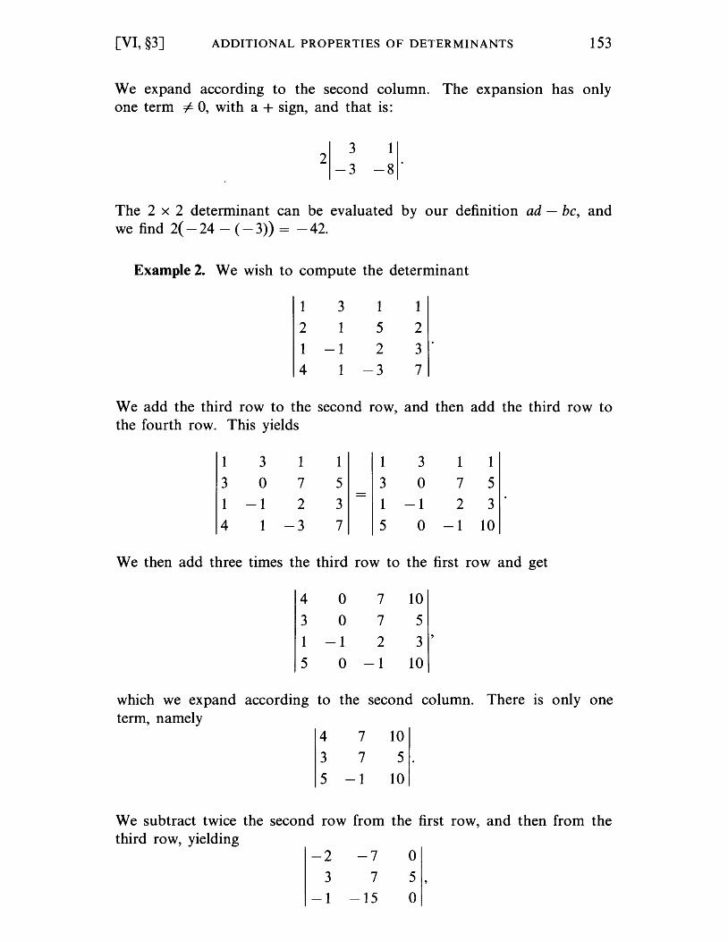
[VI, §3] ADDITIONAL PROPERTIES OF DETERMINANTS 153
We expand according to the second column. The expansion has only one term =1= 0, with a + sign, and that is:
2 3 1 -3 -8
The 2 x 2 determinant can be evaluated by our definition ad - be, and we find 2{ -24 - (-3») = -42.
Example 2. We wish to compute the determinant
1 3 1 1 2 1 5 2 1 -1 2 3 4 1 -3 7
We add the third row to the second row, and then add the third row to the fourth row. This yields
1 3 1 1 1 3 1 1 3 0 7 5 3 0 7 5 1 -1 2 3 1 -1 2 3 4 1 -3 7 5 0 -1 10
We then add three times the third row to the first row and get
4 0 7 10
307 5 1 -1 2 3 '
5 0 -1 10
which we expand according to the second column. There IS only one term, namely
4 7 10
3 7 5 .
5 -1 10
We subtract twice the second row from the first row, and then from the third row, yielding
-2 -7 0
3 7 5 ,
-1 -15 0
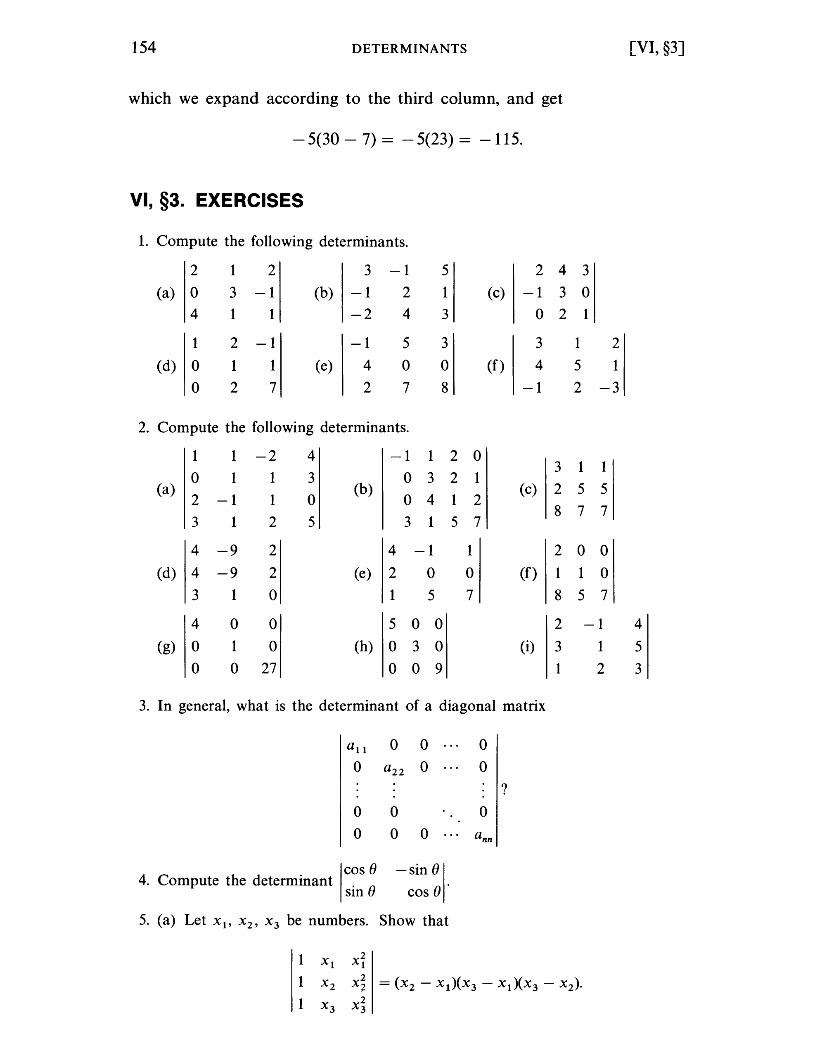
154 DETERMINANTS [VI, §3]
which we expand according to the third column, and get
-5(30 -7) = -5(23) = -115.
VI, §3. EXERCISES
1. Compute the following determinants.
2 1 2 3 -1 5 2 4 3
(a) 0 3 -1 (b) -1 2 1 (c) -1 3 0 4 1 1 -2 4 3 0 2 1
1 2 -1 -1 5 3 3 1 2
(d) 0 1 1 (e) 4 0 0 (f) 4 5 1
0 2 7 2 7 8 -1 2 -3
2. Compute the following determinants.
1 1 -2 4 -1 1 2 0 3 1 1
0 1 1 3 0 3 2 1 (a) (b) (c) 2 5 5
2 -1 1 0 0 4 1 2 8 7 7
3 1 2 5 3 1 5 7
4 -9 2 4 -1 1 2 0 0
(d) 4 -9 2 (e) 2 0 0 (f) 1 1 0
3 1 0 1 5 7 8 5 7
4 0 0 5 0 0 2 -1 4
(g) 0 1 0 (h) 0 3 0 (i) 3 1 5
0 0 27 0 0 9 1 2 3
3. In general, what is the determinant of a diagonal matrix
all 0 0 0
0 a22 0 0
?
0 0 0
0 0 0 ann
4. Compute the determinant . ICOS (J
SIn e -sin (J I.
COS e 5. (a) Let Xl' X 2 , X3 be numbers. Show that
1 Xl X2 1
1 X 2 X2
2 = (X2 - X l )(X3 - X l )(X3 - X 2 )·
1 X3 X2 3
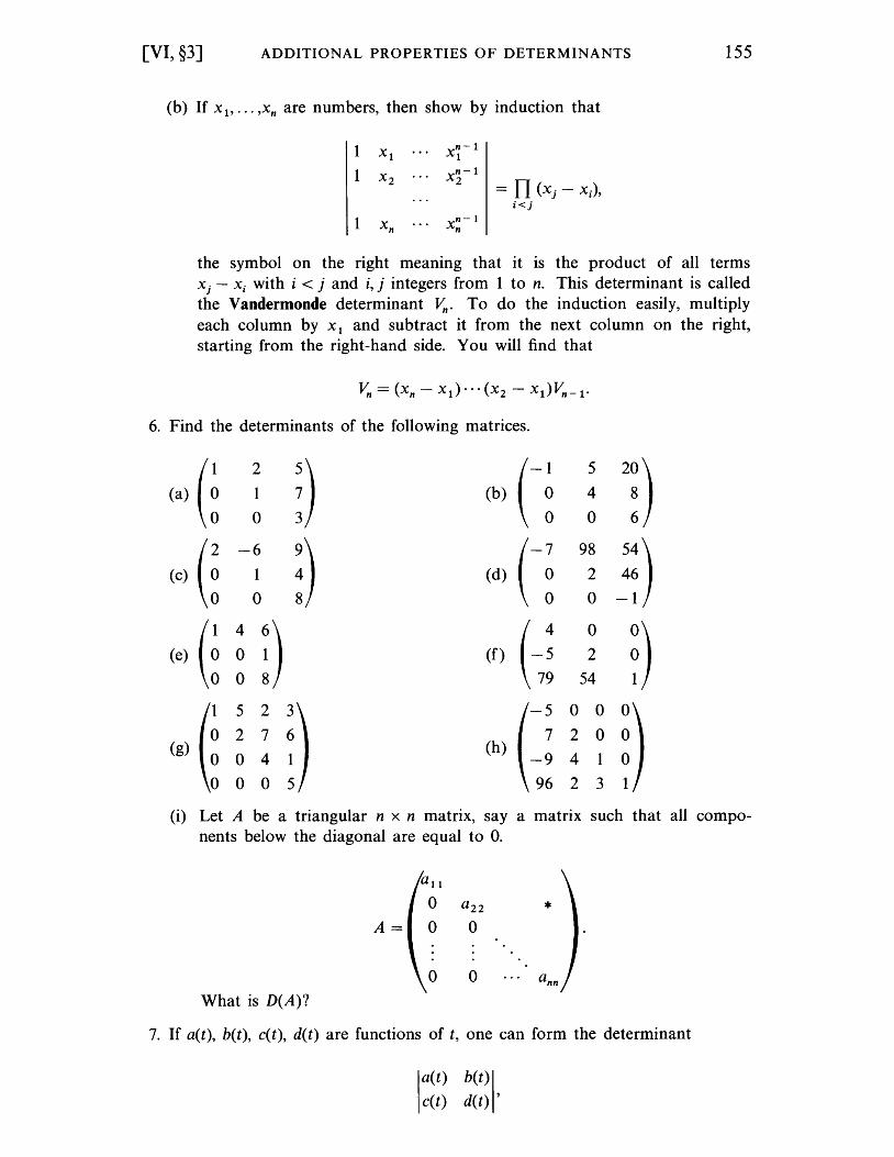
[VI, §3] ADDITIONAL PROPERTIES OF DETERMINANTS 155
(b) If Xl"" ,Xn are numbers, then show by induction that
1 Xl n-l
Xl
1 X2 n-l X2 = n (Xj - xJ,
i<j
1 Xn n-l
Xn
the symbol on the right meaning that it is the product of all terms Xj - Xi with i < j and i, j integers from 1 to n. This determinant is called the Vandermonde determinant v". To do the induction easily, multiply each column by Xl and subtract it from the next column on the right, starting from the right-hand side. You will find that
v" = (xn - x l )"'(X2 - Xl)v,,-l'
6. Find the determinants of the following matrices.
(a) (~ 2
D (-~ 5 2:) 1 (b) 4
0 0
(c) (~ -6 :) (-~
98 54) 1 (d) 2 46
0 0 -1
G 4
D (-~ 0
D (e) 0 (f) 2
0 79 54
1 5 2 3 -5 0 0
~) 0 2 7 6 7 2 0 (g)
0 0 4 1 (h)
-9 4 1
0 0 0 5 96 2 3
(i) Let A be a triangular n x n matrix, say a matrix such that all nents below the diagonal are equal to O.
o a22 * A = 0 0
o o What is D(A)?
7. If a(t), b(t), c(t), d(t) are functions of t, one can form the determinant
la(t) b(t) I c(t) d(t) ,
compo-
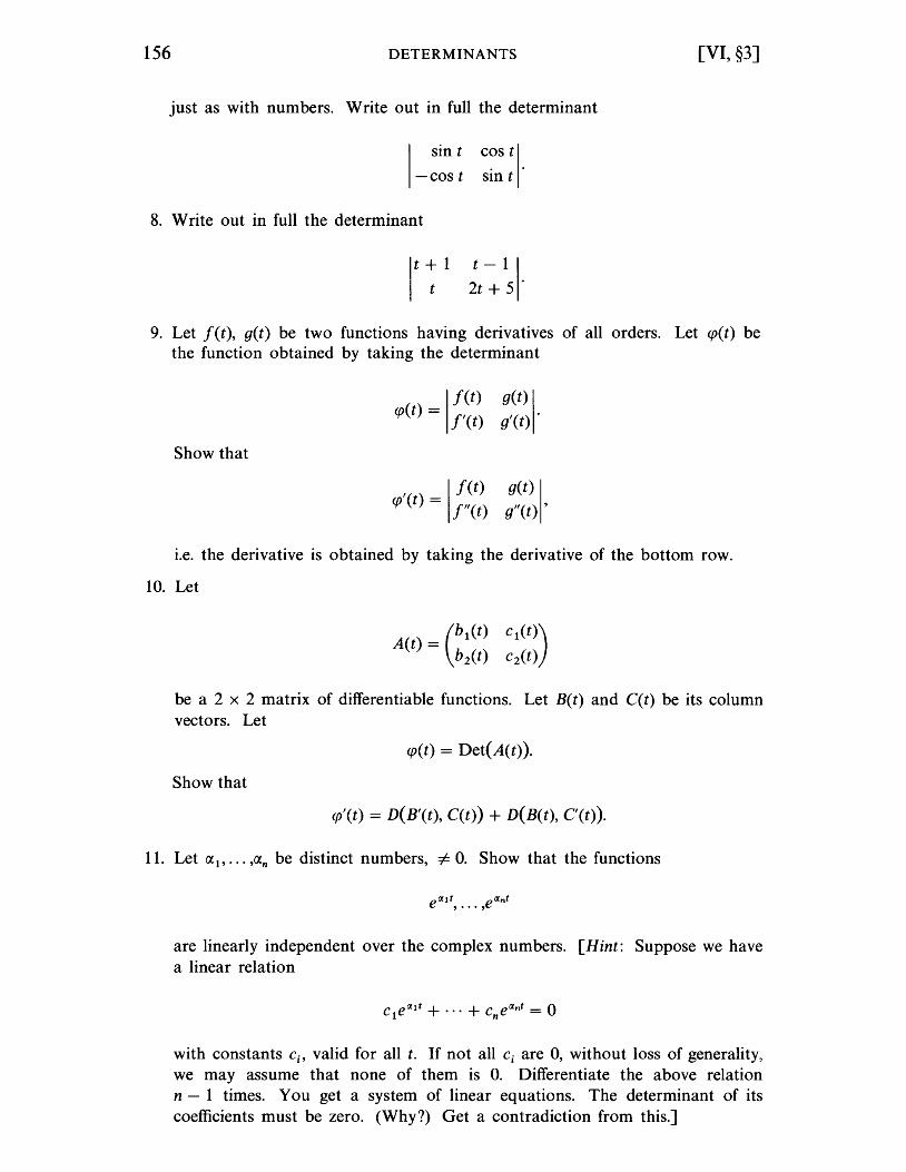
156 DETERMINANTS [VI, §3]
just as with numbers. Write out in full the determinant
I sin t cos t I
-cos t sin t .
8. Write out in full the determinant
t - 1 I 2t + 5 .
9. Let f(t), g(t) be two functions having derivatives of all orders. Let <p(t) be the function obtained by taking the determinant
I f(t) g(t) I
<p(t) = f'(t) g'(t)·
Show that
, I f(t) g(t) I <p (t) = f"(t) g"(t) ,
i.e. the derivative is obtained by taking the derivative of the bottom row.
10. Let
be a 2 x 2 matrix of differentiable functions. Let B(t) and C(t) be its column vectors. Let
<p(t) = Det(A(t).
Show that
<p'(t) = D(B'(t), C(t» + D(B(t), C'(t».
11. Let (1.1' ••• ,(1.n be distinct numbers, i= O. Show that the functions
are linearly independent over the complex numbers. [Hint: Suppose we have a linear relation
with constants Ci , valid for all t. If not all ci are 0, without loss of generality, we may assume that none of them is o. Differentiate the above relation n - 1 times. You get a system of linear equations. The determinant of its coefficients must be zero. (Why?) Get a contradiction from this.]
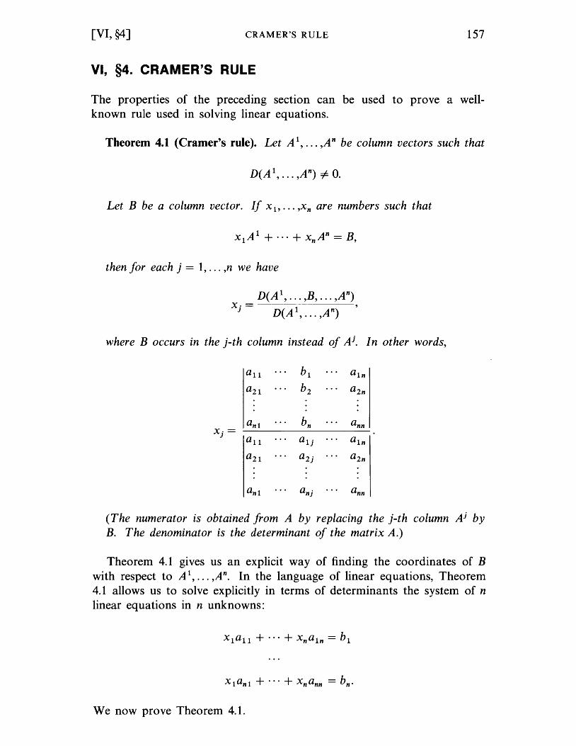
[VI, §4] CRAMER'S RULE 157
VI, §4. CRAMER'S RULE
The properties of the preceding section can be used to prove a wellknown rule used in solving linear equations.
Theorem 4.1 ( Cramer's rule). Let A l, ... ,A n be column vectors such that
Let B be a column vector. If Xl' ... ,Xn are numbers such that
then for each j = 1, ... ,n we have
D(A l, ... ,B, ... ,An) x·=-------
J D(A 1, ... ,An)
where B occurs in the j-th column instead of Ai. In other words,
all bl aln a2l b2 a2n
anl bn ann Xi =
all ali aln a2l a2i a2n
anl ani ann
(The numerator is obtained from A by replacing the j-th column Ai by B. The denominator is the determinant of the matrix A.)
Theorem 4.1 gives us an explicit way of finding the coordinates of B with respect to A l, ... ,An. In the language of linear equations, Theorem 4.1 allows us to solve explicitly in terms of determinants the system of n linear equations in n unknowns:
We now prove Theorem 4.1.
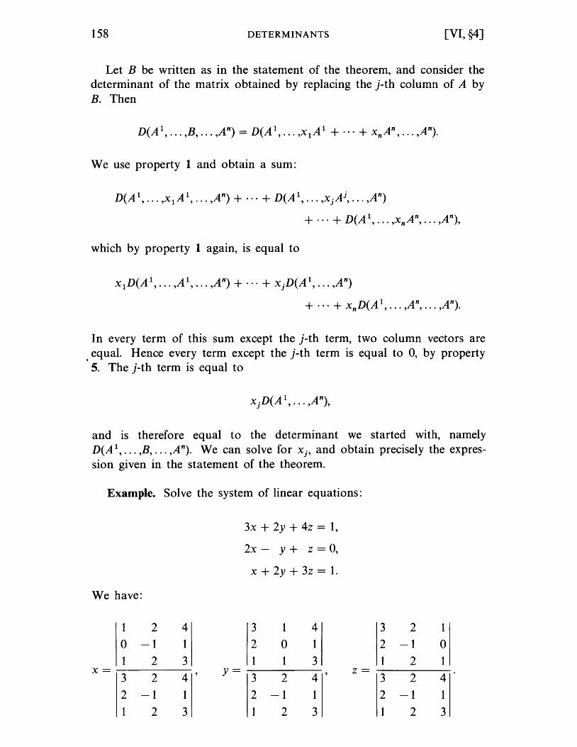
\
158 DETERMINANTS [VI, §4]
Let B be written as in the statement of the theorem, and consider the determinant of the matrix obtained by replacing the j-th column of A by B. Then
We use property 1 and obtain a sum:
D(A I, ... ,Xl A I, ... ,An) + ... + D(A I, ... ,xjAj, ... ,An)
+ ... + D(A I, ... ,xnAn, ... ,An),
which by property 1 again, is equal to
X I D(A I, ... ,A I, ... ,An) + ... + X jD(A I, ... ,A n)
+ ... + xnD(A I, ... ,An, ... ,An).
In every term of this sum except the j-th term, two column vectors are equal. Hence every term except the j-th term is equal to 0, by property 5. The j-th term is equal to
and is therefore equal to the determinant we started with, namely D(A I, ... ,B, ... ,An). We can solve for Xj' and obtain precisely the expression given in the statement of the theorem.
Example. Solve the system of linear equations:
3x + 2y + 4z = 1,
2x - y+ z = 0,
X + 2y + 3z = 1.
We have:
1 2 4 3 1 4 3 2 1
0 -1 1 2 0 1 2 -1 0 1 2 3 1 1 3 1 2 1
X= 3 2 4 '
y= 3 2 4'
Z= 3 2 4
2 -1 1 2 -1 1 2 -1 1
1 2 3 2 3 2 3
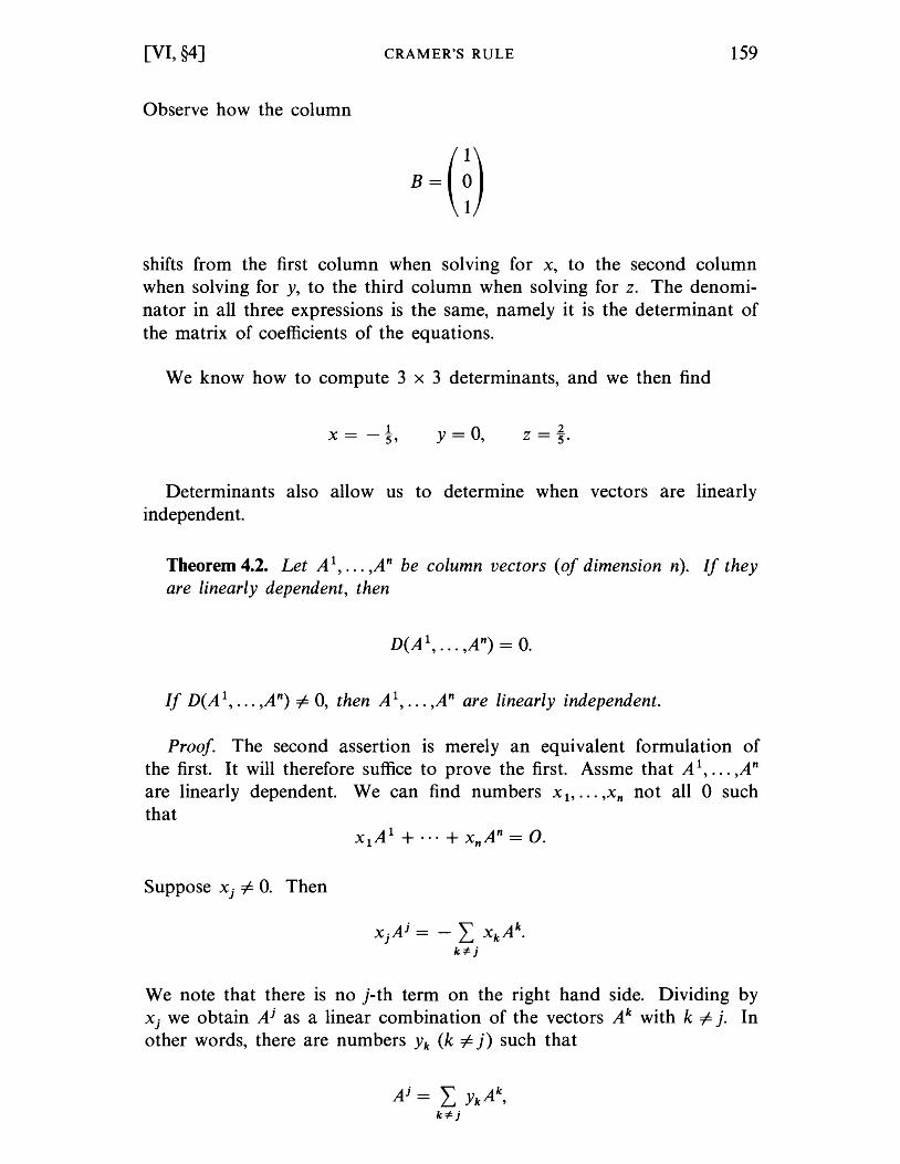
[VI, §4] CRAMER'S RULE 159
Observe how the column
B =(~) shifts from the first column when solving for x, to the second column when solving for y, to the third column when solving for z. The denominator in all three expressions is the same, namely it is the determinant of the matrix of coefficients of the equations.
We know how to compute 3 x 3 determinants, and we then find
x = -!, y = 0, z =~.
Determinants also allow us to determine when vectors are linearly independent.
Theorem 4.2. Let AI, ... ,An be column vectors (of dimension n). If they are linearly dependent, then
If D(A 1, ... ,An) =1= 0, then AI, ... ,An are linearly independent.
Proof. The second assertion is merely an equivalent formulation of the first. It will therefore suffice to prove the first. Assme that AI, ... ,An are linearly dependent. We can find numbers Xb ... ,xn not all 0 such that
Suppose xi =1= O. Then
We note that there is no j-th term on the right hand side. Dividing by xi we obtain Ai as a linear combination of the vectors Ak with k =1= j. In other words, there are numbers Yk (k =1= j) such that
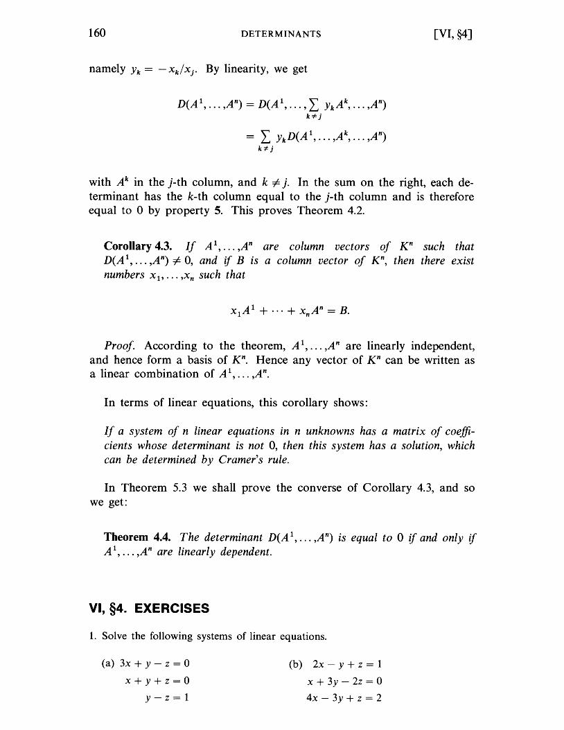
160 DETERMINANTS
namely Yk = -xk/xj • By linearity, we get
D( A 1 , ... ,An) = D( A 1 , ... , L Y k A k, ... ,An) k*j
= L YkD(A1, ... ,Ak, ... ,An) k*j
[VI, §4]
with Ak in the j-th column, and k =1= j. In the sum on the right, each determinant has the k-th column equal to the j-th column and is therefore equal to 0 by property 5. This proves Theorem 4.2.
Corollary 4.3. If A 1 , ... ,An are column vectors of Kn such that D( A 1, ... ,An) =1= 0, and if B is a column vector of Kn, then there exist numbers Xl' ... ,xn such that
Proof. According to the theorem, A 1, ... ,An are linearly independent, and hence form a basis of Kn. Hence any vector of K n can be written as a linear combination of A 1 , ... ,An.
In terms of linear equations, this corollary shows:
If a system of n linear equations in n unknowns has a matrix of coefficients whose determinant is not 0, then this system has a solution, which can be determined by Cramer's rule.
In Theorem 5.3 we shall prove the converse of Corollary 4.3, and so we get:
Theorem 4.4. The determinant D(A 1, ... ,An) is equal to 0 if and only if A 1, ... ,An are linearly dependent.
VI, §4. EXERCISES
1. Solve the following systems of linear equations.
(a) 3x + y - z = 0
x+y+z=O
y-z=l
(b) 2x - y + z = 1
x + 3y - 2z = 0
4x - 3y + z = 2
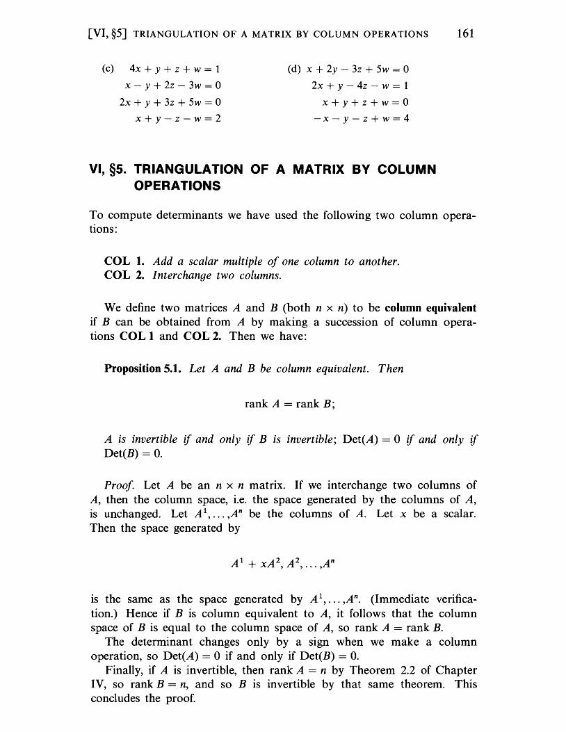
[VI, §5] TRIANGULATION OF A MATRIX BY COLUMN OPERATIONS 161
(c) 4x + y + z + w = 1
x - y + 2z - 3w = 0
2x + y + 3z + 5w = 0
x+y-z-w=2
(d) x + 2y - 3z + 5w = 0
2x + y - 4z - w = 1
x+y+z+w=o
-x-y-z+w=4
VI, §5. TRIANGULATION OF A MATRIX BY COLUMN OPERATIONS
To compute determinants we have used the following two column operations:
COL 1. Add a scalar multiple of one column to another. COL 2. Interchange two columns.
We define two matrices A and B (both n x n) to be column equivalent if B can be obtained from A by making a succession of column operations COL 1 and COL 2. Then we have:
Proposition 5.1. Let A and B be column equivalent. Then
rank A = rank B;
A is invertible if and only if B is invertible; Det(A) = 0 if and only if Det(B) = O.
Proof. Let A be an n x n matrix. If we interchange two columns of A, then the column space, i.e. the space generated by the columns of A, is unchanged. Let A 1, ... ,An be the columns of A. Let x be a scalar. Then the space generated by
is the same as the space generated by A 1, ... ,An. (Immediate verification.) Hence if B is column equivalent to A, it follows that the column space of B is equal to the column space of A, so rank A = rank B.
The determinant changes only by a sign when we make a column operation, so Det(A) = 0 if and only if Det(B) = o.
Finally, if A is invertible, then rank A = n by Theorem 2.2 of Chapter IV, so rank B = n, and so B is invertible by that same theorem. This concludes the proof.
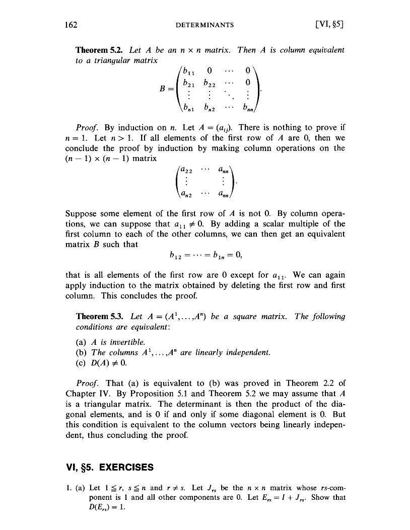
162 DETERMINANTS [VI, §5]
Theorem 5.2. Let A be an n x n matrix. Then A is column equivalent to a triangular matrix
b 11 0 0 b21 b22 0
B=
bn1 bn2 bnn
Proof. By induction on n. Let A = (a ij). There is nothing to prove if n = 1. Let n > 1. If all elements of the first row of A are 0, then we conclude the proof by induction by making column operations on the (n - 1) x (n - 1) matrix
Suppose some element of the first row of A is not O. By column operations, we can suppose that all =/; O. By adding a scalar multiple of the first column to each of the other columns, we can then get an equivalent matrix B such that
b12 = ... = b1n = 0,
that is all elements of the first row are 0 except for all. We can again apply induction to the matrix obtained by deleting the first row and first column. This concludes the proof.
Theorem 5.3. Let A = (A 1 , ... ,An) be a square matrix. T he following conditions are equivalent:
(a) A is invertible. (b) The columns A 1, ... ,An are linearly independent. (c) D(A) =/; O.
Proof. That (a) is equivalent to (b) was proved in Theorem 2.2 of Chapter IV. By Proposition 5.1 and Theorem 5.2 we may assume that A is a triangular matrix. The determinant is then the product of the diagonal elements, and is 0 if and only if some diagonal element is O. But this condition is equivalent to the column vectors being linearly independent, thus concluding the proof.
VI, §5. EXERCISES
1. (a) Let 1 ~ r, s ~ nand r i= s. Let J rs be the n x n matrix whose rs-component is 1 and all other components are O. Let Ers = I + J rs. Show that D(Ers ) = 1.
[VI, §6] PERMUTATIONS 163
(b) Let A be an n x n matrix. What is the effect of multiplying ErsA? of multiplying AErs?
2. In the proof of Theorem 5.3, we used the fact that if A is a triangular matrix, then the column vectors are linearly independent if .and only if all diagonal elements are =1= O. Give the details of the proof of this fact.
VI, §6. PERMUTATIONS
We shall deal only with permutations of the set of integers {I, ... ,n}, which we denote by J n' By definition, a permutation of this set is a map
a: {1, ... ,n} ~ {I, ... ,n}
of J n into itself such that, if i, j E J nand i i= j, then a(i) i= a(j). Thus a permutation is a bijection of J n with itself. If a is such a permutation, then the set of integers
{ a( 1), ... ,a( n ) }
has n distinct elements, and hence consists again of the integers 1, ... ,n in a different arrangement. Thus to each integer j E J n there exists a unique integer k such that a(k) = j. We can define the inverse permutation, denoted by a - 1, as the map
such that a- l(k) = unique integer j E J n such that a(j) = k. If a, ! are permutations of I n , then we can form their composite map
a O!,
and this map will again be a permutation. We shall usually omit the small circle, and write a! for the composite map. Thus
By definition, for any permutation a, we have
and
where id is the identity permutation, that is, the permutation such that id(i) = i for all i = 1, ... ,no
164 DETERMINANTS [VI, §6]
If a 1, ••. ,ar are permutations of J n' then the inverse of the composite map
a1
••• ar
is the permutation
This is trivially seen by direct multiplication. A transposition is a permutation which interchanges two numbers and
leaves the others fixed. The inverse of a transposition r is obviously equal to the transposition r itself, so that r2 = ide
Proposition 6.1. Every permutation of J n can be expressed as a product of transpositions.
Proof. We shall prove our assertion by induction on n. For n = 1, there is nothing to prove. Let n > 1 and assume the assertion proved for n - 1. Let a be a permutation of J n. Let a(n) = k. If k =1= n let r be the transposition of J n such that r( k) = n, r( n) = k. If k = n, let r = ide Then ra is a permutation such that
ra(n) = r(k) = n.
In other words, ra leaves n fixed. We may therefore view ra as a permutation of J n - l' and by induction, there exist transpositions r 1, ... ,r s of I n - 1 , leaving n fixed, such that
ra = r 1 ... rs. We can now write
-1 a = r r 1 ... r s = rr 1 ... r s'
thereby proving our proposition.
Example 1. A permutation a of the integers {I, ... ,n} is denoted by
Thus
[VI, §6] PERMUTATIONS 165
denotes the permutation a such that a(l) = 2, a(2) = 1, and a(3) = 3. This permutation is in fact a transposition. If a' is the permutation
[1 2 3J 3 12'
then aa' = a 0 a' is the permutation such that
so that we can write
aa'(I) = a(a'(I») = a(3) = 3,
aa'(2) = a(a'(2») = a(l) = 2,
aa'(3) = a(a'(3») = a(2) = 1,
[1 2 3J
aa' = 3 2 1 .
Furthermore, the inverse of a' is the permutation
[1 2 3J 231
as is immediately determined from the definitions: Since a'(I) = 3, we must have a'-l(3) = 1. Since a'(2) = 1, we must have a'-l(l) = 2. Finally, since a'(3) = 2, we must have a'-l(2) = 3.
Example 2. We wish to express the permutation
= [1 2 3J a 312
as a product of transpositions. Let r be the transposItIon which interchanges 3 and 1, and leaves 2 fixed. Then using the definition, we find that
[1 2 3J
ra = 1 3 2
so that ra is a transposition, which we denote by r'. We can then write ra = r', so that
because r- 1 = r. This is the desired product.
166 DETERMINANTS
Example 3. Express the permutation
_ [1 2 3 41J a - 2 3 4
as a product of transpositions.
[VI, §6]
Let r 1 be the transposition which interchanges 1 and 2, and leaves 3, 4 fixed. Then
2 3 4J. 342
Now let r 2 be the transposition which interchanges 2 and 3, and leaves 1, 4 fixed. Then
2 3 4J 2 4 3 '
and we see that r 2 r 1 a is a transposition, which we may denote by r 3' Then we get r 2 r 1 a = r3 so that
Proposition 6.2. To each permutation a of J n it is possible to assign a sign 1 or -1, denoted by E(a), satisfying the following conditions:
(a) If r is a transposition, then E(r) = -1. (b) If a, a' are permutations of J n' then
E(aa') = E(a)E(a').
In fact, if A = (A 1, ... ,An) is an n x n matrix, then E(a) can be defined by the condition
Proof. Observe that (Au(l), ... ,Au(n» is simply a different ordering from (A 1, ... ,An). Let a be a permutation of J n' Then
and the sign + or - is determined by a, and does not depend on A 1, ... ,An. Indeed, by making a succession of transpositions, we can return (Au(l), ... ,Au(n» to the standard ordering (A 1, ... ,An), and each transposition changes the determinant by a sign. Thus we may define
D( A u( 1) A u(n» E(a) = ---' -' '-' -' --
D(A 1, ... ,An)
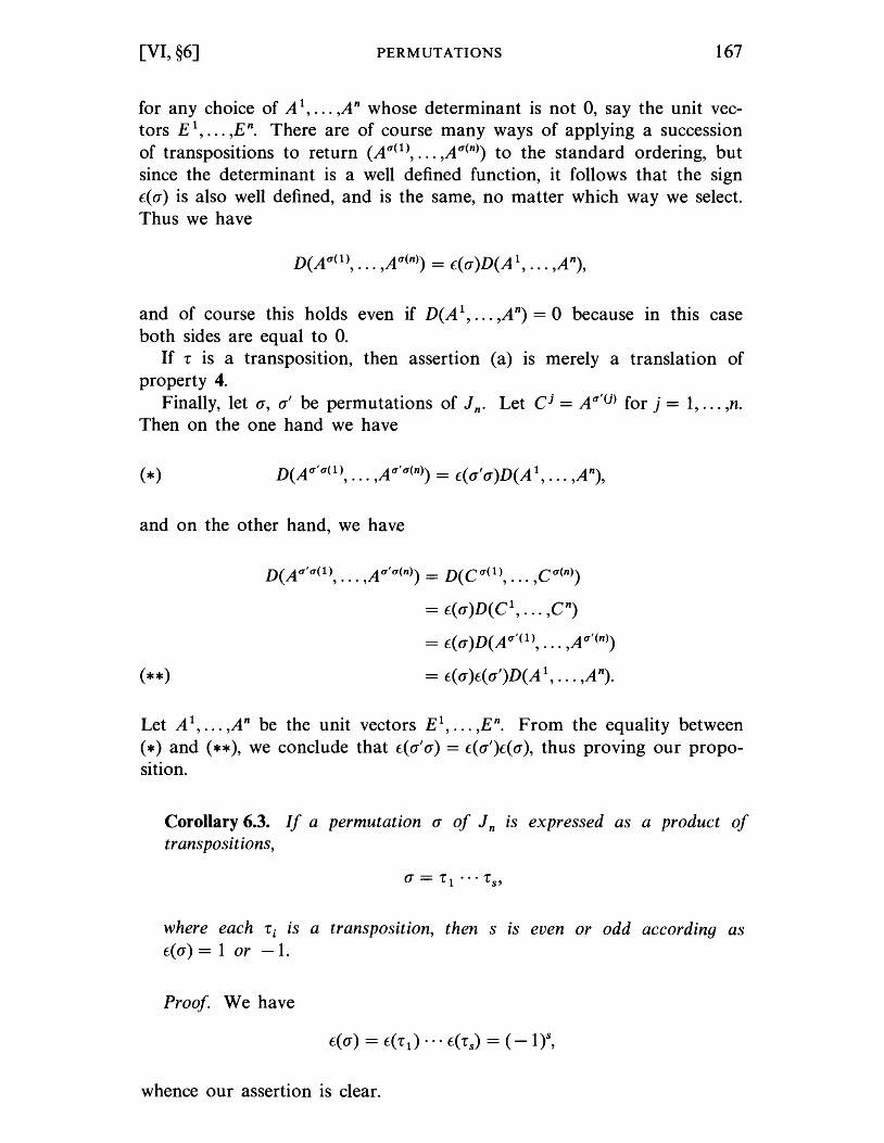
[VI, §6] PERMUTATIONS 167
for any choice of A 1, ... ,A n whose determinant is not 0, say the unit vectors E 1
, ••• ,En. There are of course many ways of applying a succession of transpositions to return (Au(1), ... ,Au(n») to the standard ordering, but since the determinant is a well defined function, it follows that the sign E(a) is also well defined, and is the same, no matter which way we select. Thus we have
and of course this holds even if D(A 1, ... ,An) = 0 because In this case both sides are equal to O.
If r is a transposition, then assertion (a) is merely a translation of property 4.
Finally, let a, a' be permutations of J n. Let C i = AU'U) for j = 1, ... ,no Then on the one hand we have
and on the other hand, we have
= E(a)D(C 1, ••• ,cn)
= E( a )D( A u'( 1), ... ,A u'(n»)
= E( a )E( a')D( A 1 , ... ,A n).
Let A 1, ... ,An be the unit vectors E 1, ••• ,En. From the equality between
(*) and (**), we conclude that E(a' a) = E(a')E(a), thus proving our proposition.
Corollary 6.3. If a permutation a of J n is expressed as a product of transpositions,
where each r i is a transposition, then s is even or odd according as E( a) = 1 or - 1.
Proof. We have
whence our assertion is clear.
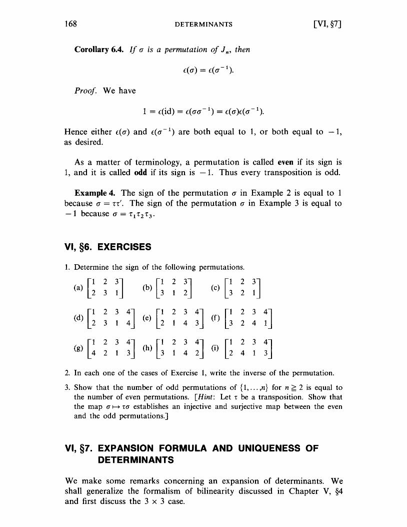
168 DETERMINANTS [VI, §7]
Corollary 6.4. If a is a permutation of J n' then
Proof. We have
Hence either E(a) and E(a- 1) are both equal to 1, or both equal to -1,
as desired.
As a matter of terminology, a permutation is called even if its sign is 1, and it is called odd if its sign is -1. Thus every transposition is odd.
Example 4. The sign of the permutation a in Example 2 is equal to 1 because a = 7:7:'. The sign of the permutation a in Example 3 is equal to -1 because a = 7: 1 7: 2 7: 3 ,
VI, §6. EXERCISES
1. Determine the sign of the following permutations.
(a) [~ ~ ~J (b) [~ ~ ~J (c) [~ ~ ~J
[1
2 3 44J [1
2 3 43J [31
2 3 41 J (d) 2 3 1 (e) 2 1 4 (f) 2 4
(g) [~ ~ ~ ~J (h) [! ~ ! ~J (i) G ~ ~ ~J 2. In each one of the cases of Exercise 1, write the inverse of the permutation.
3. Show that the number of odd permutations of {1, ... ,n} for n ~ 2 is equal to the number of even permutations. [Hint: Let! be a transposition. Show that the map (J I---+!(J establishes an injective and surjective map between the even and the odd permutations.]
VI, §7. EXPANSION FORMULA AND UNIQUENESS OF DETERMINANTS
We make some remarks concerning an expansion of determinants. We shall generalize the formalism of bilinearity discussed in Chapter V, §4 and first discuss the 3 x 3 case.
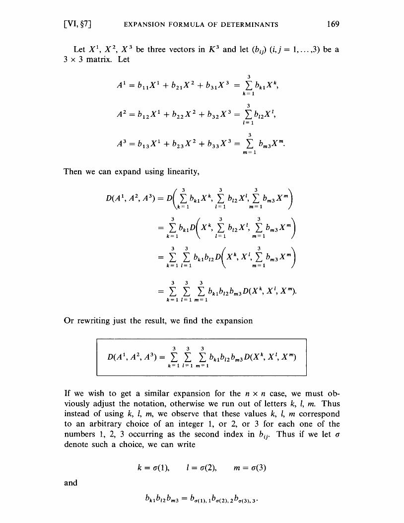
[VI, §7] EXPANSION FORMULA OF DETERMINANTS 169
Let Xl, X 2, X 3 be three vectors in K3 and let (bij) (i,j = 1, ... ,3) be a 3 x 3 matrix. Let
3
Al = bllX I + b2l X 2 + b3l X 3 - L bklX\ k=l
3
A2 = bl2 X l + b22 X 2 + b32 X 3 = L b,2X ', 1= I
3
A 3 = bl3 X l + b23 X 2 + b33 X 3 = L bm3xm. m=l
Then we can expand using linearity,
D(A\ A2, A
3) = D(t
lbklX\ Itl bl2XI'mtlbm3xm)
- ktlbklD( xk, Itl bl2 XI, mtlbm3 xm)
- ktl Jl bkl bl2 D( X\XI'mtlbm3xm) 3 3 3
- L L L bklb'2bm3D(Xk, X', xm). k=l'=l m=l
Or rewriting just the result, we find the expansion
3 3 3
D(A\ A 2, A 3) = L L L bklb'2bm3D(Xk, X', xm) k=11=1 m=l
If we wish to get a similar expansion for the n x n case, we must obviously adjust the notation, otherwise we run out of letters k, 1, m. Thus instead of using k, 1, m, we observe that these values k, 1, m correspond to an arbitrary choice of an integer 1, or 2, or 3 for each one of the numbers 1, 2, 3 occurring as the second index in b ij. Thus if we let (J denote such a choice, we can write
k = (J(I), 1 = (J(2), m = (J(3)
and
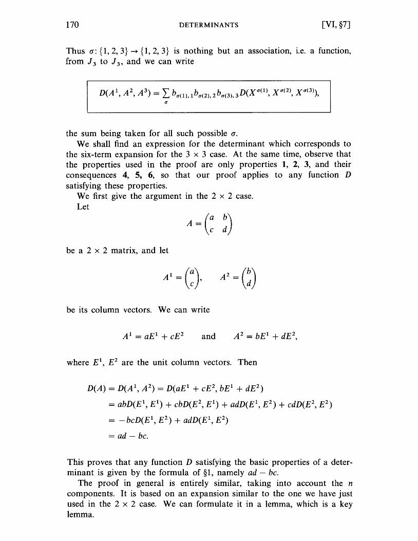
170 DETERMINANTS [VI, §7]
Thus (1: {I, 2, 3} ~ {I, 2, 3} is nothing but an association, I.e. a function, from J 3 to J 3' and we can write
the sum being taken for all such possible (1.
We shall find an expression for the determinant which corresponds to the six-term expansion for the 3 x 3 case. At the same time, observe that the properties used in the proof are only properties 1, 2, 3, and their consequences 4, 5, 6, so that our proof applies to any function D satisfying these properties.
We first give the argument in the 2 x 2 case. Let
A = (: !) be a 2 x 2 matrix, and let
be its column vectors. We can write
and
where El, E2 are the unit column vectors. Then
D(A) = D(A 1, A2) = D(aEl + eE2, bEl + dE2)
= abD(E1, El) + ebD(E2, El) + adD(E1, E2) + edD(E2, E2)
= -beD(E 1, E2) + adD(El, E2)
= ad - be.
This proves that any function D satisfying the basic properties of a determinant is given by the formula of §l, namely ad - be.
The proof in general is entirely similar, taking into account the n components. It is based on an expansion similar to the one we have just used in the 2 x 2 case. We can formulate it in a lemma, which is a key lemma.
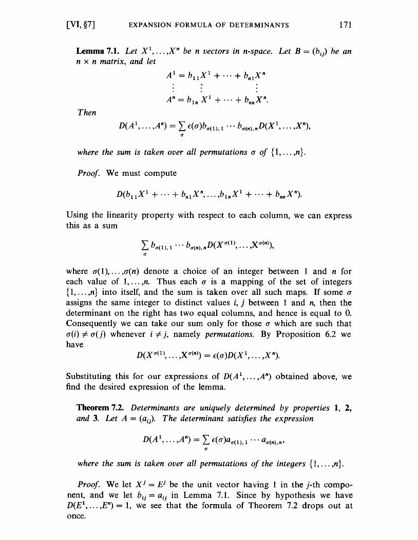
[VI, §7] EXPANSION FORMULA OF DETERMINANTS 171
Lemma 7.1. Let Xl, ... ,xn be n vectors in n-space. Let B = (bij) be an n x n matrix, and let
Al=b X 1 + ... +b xn 11 nl
Then
D(A 1, ... ,An) = I £(a)bu(1), 1 ••• bu(n),n D(X 1, ••• ,Xn),
where the sum is taken over all permutations a of {1, ... ,n}.
Proof. We must compute
Using the linearity property with respect to each column, we can express this as a sum
L bu(1), 1 ••. bu(n),nD(Xu(1), ... ,xu(n», u
where a(1), ... ,a(n) denote a choice of an integer between 1 and n for each value of 1, ... ,no Thus each a is a mapping of the set of integers {1, ... ,n} into itself, and the sum is taken over all such maps. If some a assigns the same integer to distinct values i, j between 1 and n, then the determinant on the right has two equal columns, and hence is equal to O. Consequently we can take our sum only for those a which are such that a(i) 1= a( j) whenever i 1= j, namely permutations. By Proposition 6.2 we have
D(xu(l), ... ,xu(n» = £(a)D(Xl, ... ,xn).
Substituting this for our expressions of D(A 1, ... ,An) obtained above, we find the desired expression of the lemma.
Theorem 7.2. Determinants are uniquely determined by properties 1, 2, and 3. Let A = (a ij). The determinant satisfies the expression
D(A 1, ... ,An) = L £(a)au(l), 1 ... au(n),n'
where the sum is taken over all permutations of the integers {1, ... ,n}.
Proof. We let X j = Ej be the unit vector having 1 in the j-th component, and we let bij = aij in Lemma 7.1. Since by hypothesis we have D(Et, ... ,En) = 1, we see that the formula of Theorem 7.2 drops out at once.
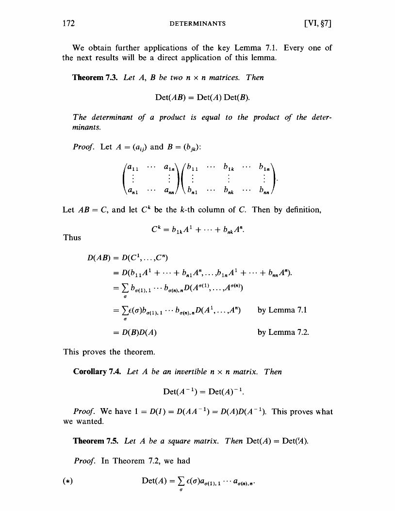
172 DETERMINANTS [VI, §7]
We obtain further applications of the key Lemma 7.1. Everyone of the next results will be a direct application of this lemma.
Theorem 7.3. Let A, B be two n x n matrices. Then
Det(AB) = Det(A) Det(B).
The determinant of a product is equal to the product of the determinants.
Proof. Let A = (aij) and B = (b jk ):
Let AB = C, and let C k be the k-th column of C. Then by definition,
Thus
D(AB) = D(C I, ... ,C n)
= D(bIIAI + ... + bnIAn, ... ,bInAI + ... + bnnAn).
- ~ b ... b D(AO'(1) AO'(n») - ~ 0'(1), I O'(n), n , ••• ,
0'
by Lemma 7.1
=D(B)D(A) by Lemma 7.2.
This proves the theorem.
Corollary 7.4. Let A be an invertible n x n matrix. Then
Proof. We have 1 = D(I) = D(AA- I) = D(A)D(A- I). This proves ,,'hat we wanted.
Theorem 7.5. Let A be a square matrix. Then Det(A) = Det(~).
Proof. In Theorem 7.2, we had
Det(A) = L £(a)aO'(I), I ... aO'(n),n·
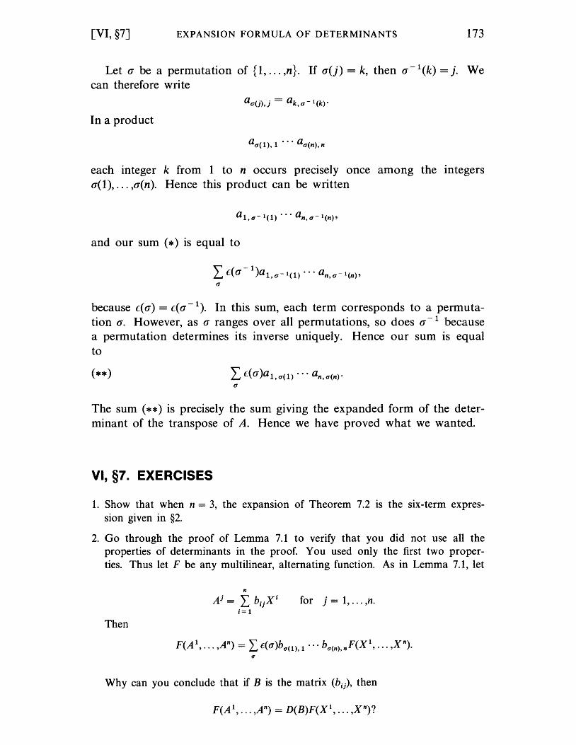
[VI, §7] EXPANSION FORMULA OF DETERMINANTS 173
Let a be a permutation of {1, ... ,n}. If a(j) = k, then a- 1(k) = j. We can therefore write
In a product
aO'( 1), 1 ••• aO'(n), n
each integer k from 1 to n occurs precisely once among the integers a(1), ... ,a(n). Hence this product can be written
and our sum (*) is equal to
L (a- 1 )a 1 ,0'-1(1) ••• an,O'-I(n)' 0'
because (a) = (a- 1). In this sum, each term corresponds to a permuta
tion a. However, as a ranges over all permutations, so does a - 1 because a permutation determines its inverse uniquely. Hence our sum is equal to
L (a)a 1,0'(1) ••• an, O'(n)· 0'
The sum (**) is precisely the sum giving the expanded form of the determinant of the transpose of A. Hence we have proved what we wanted.
VI, §7. EXERCISES
1. Show that when n = 3, the expansion of Theorem 7.2 is the six-term expression given in §2.
2. Go through the proof of Lemma 7.1 to verify that you did not use all the properties of determinants in the proof. You used only the first two properties. Thus let F be any multilinear, alternating function. As in Lemma 7.1, let
Then
n
Ai = L biiX i i= 1
for j = 1, ... ,no
F(A 1, ... ,An) = L f(a)bO'(1), 1 ••• bO'(n),nF(Xt, ... ,xn). 0'
Why can you conclude that if B is the matrix (b i), then
F(A 1, ... ,An) = D(B)F(Xl, ... ,xn)?
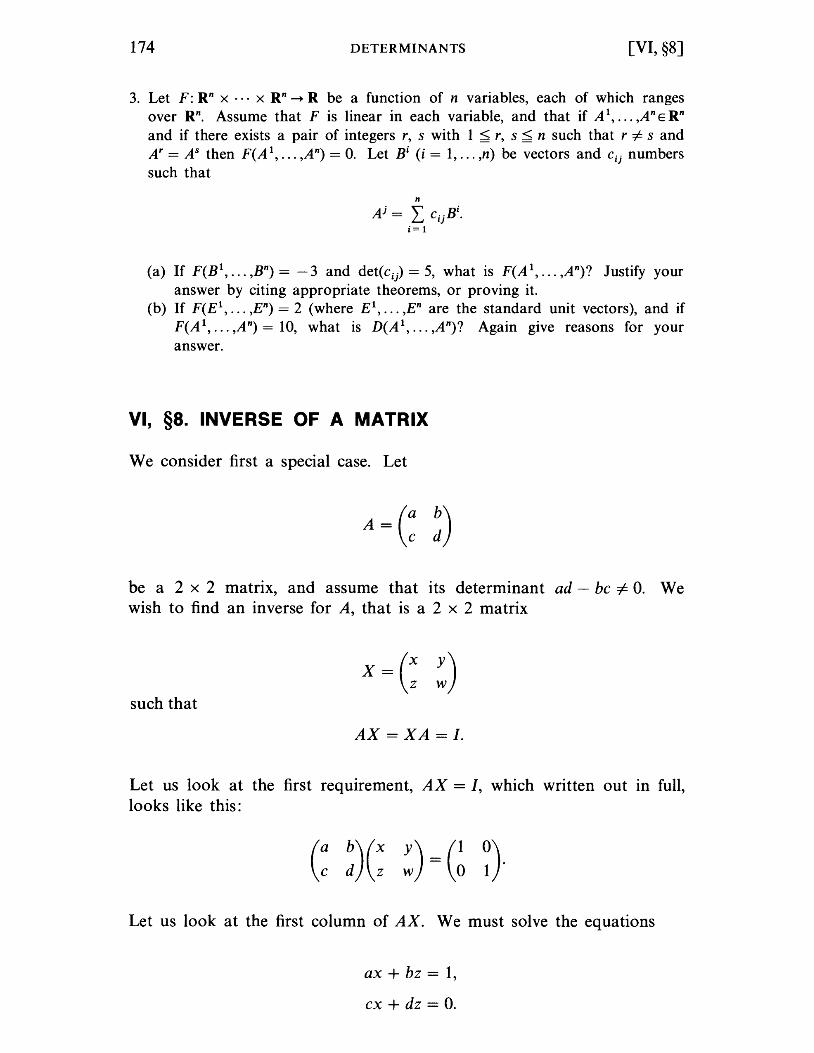
174 DETERMINANTS [VI, §8]
3. Let F: Rn x ... x Rn ~ R be a function of n variables, each of which ranges over Rn. Assume that F is linear in each variable, and that if A1, ... ,An E Rn and if there exists a pair of integers r, s with 1 ~ r, s ~ n such that r # sand Ar = AS then F(A 1, ... ,An) = O. Let Bi (i = 1, ... ,n) be vectors and cij numbers such that
n
Aj = L cijBi•
i= 1
(a) If F(B 1, ••• ,Bn) = - 3 and det(c i) = 5, what is F(A 1, ... ,An)? Justify your
answer by citing appropriate theorems, or proving it. (b) If F(E 1
, ••• ,En) = 2 (where E 1, ••• ,En are the standard unit vectors), and if
F(A 1, ... ,An) = 10, what is D(A 1, ... ,An)? Again give reasons for your answer.
VI, §8. INVERSE OF A MATRIX
We consider first a special case. Let
A = (: !) be a 2 x 2 matrix, and assume that its determinant ad - be #- O. We wish to find an inverse for A, that is a 2 x 2 matrix
such that
AX=XA=I.
Let us look at the first requirement, AX = I, which written out in full, looks like this:
Let us look at the first column of AX. We must solve the equations
ax + bz = 1,
ex + dz = O.
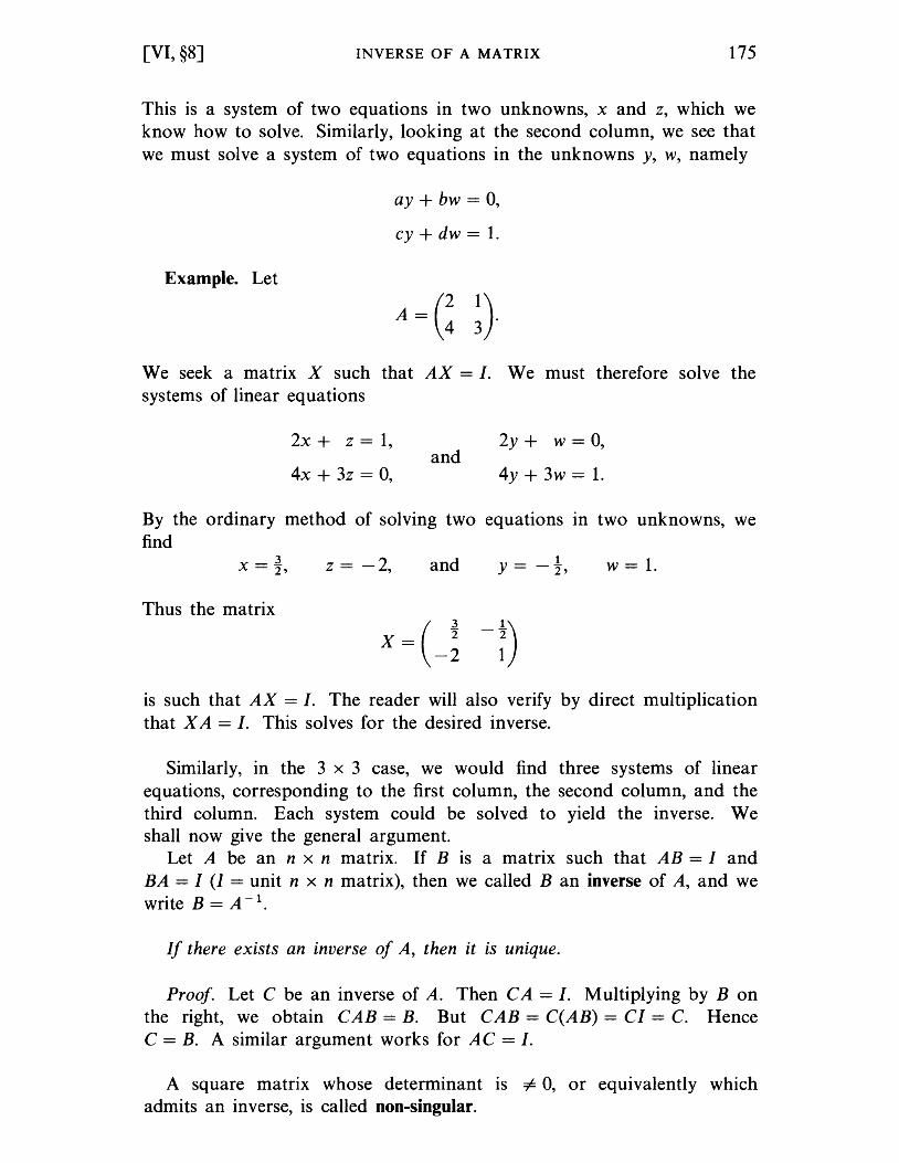
[VI, §8] INVERSE OF A MATRIX 175
This is a system of two equations in two unknowns, x and z, which we know how to solve. Similarly, looking at the second column, we see that we must solve a system of two equations in the unknowns y, W, namely
Example. Let
ay + bw = 0,
cy + dw = 1.
A = (2 1) 43'
We seek a matrix X such that AX = I. We must therefore solve the systems of linear equations
2x + z = 1,
4x + 3z = 0, and
2y + w = 0,
4y + 3w = 1.
By the ordinary method of solving two equations in two unknowns, we find
z = -2, and y = -!, w=1.
Thus the matrix
X=( ! -!) -2 1
is such that AX = I. The reader will also verify by direct multiplication that X A = I. This solves for the desired inverse.
Similarly, in the 3 x 3 case, we would find three systems of linear equations, corresponding to the first column, the second column, and the third column. Each system could be solved to yield the inverse. We shall now give the general argument.
Let A be an n x n matrix. If B is a matrix such that AB = I and BA = I (1 = unit n x n matrix), then we called B an inverse of A, and we write B = A -1.
If there exists an inverse of A, then it is unique.
Proof. Let C be an inverse of A. Then CA = I. Multiplying by B on the right, we obtain CAB = B. But CAB = C(AB) = CI = C. Hence C = B. A similar argument works for AC = I.
A square matrix whose determinant is =1= 0, or equivalently which admits an inverse, is called non-singular.
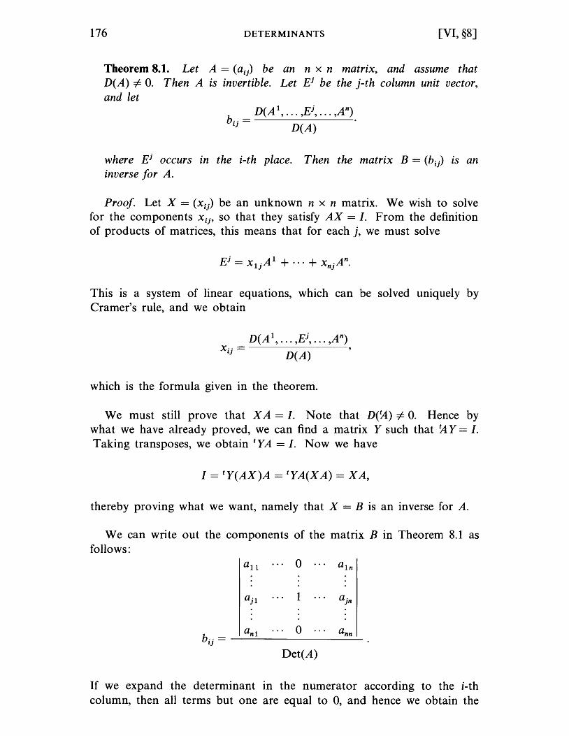
176 DETERMINANTS [VI, §8]
Theorem 8.1. Let A = (aij) be an n x n matrix, and assume that D(A) 1= o. Then A is invertible. Let Ej be the j-th column unit vector, and let
D(A 1, ... ,Ej, ... ,An) b··= .
lJ D(A)
where Ej occurs in the i-th place. Then the matrix B = (bij) is an inverse for A.
Proof. Let X = (xij) be an unknown n x n matrix. We wish to solve for the components Xij' so that they satisfy AX = I. From the definition of products of matrices, this means that for each j, we must solve
This is a system of linear equations, which can be solved uniquely by Cramer's rule, and we obtain
D(A)
which is the formula given in the theorem.
We must still prove that XA = I. Note that D(~) 1= O. Hence by what we have already proved, we can find a matrix Y such that ~ Y = I. Taking transposes, we obtain tYA = I. Now we have
I = tY(AX)A = tYA(XA) = XA,
thereby proving what we want, namely that X = B is an inverse for A.
We can write out the components of the matrix B in Theorem 8.1 as follows:
all 0 a ln
ajl 1 ajn
b··= an! 0 a"n
lJ
Det(A)
If we expand the determinant in the numerator according to the i-th column, then all terms but one are equal to 0, and hence we obtain the
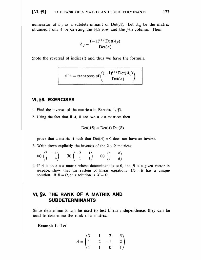
[VI, §9] THE RANK OF A MATRIX AND SUBDETERMINANTS 177
numerator of b ij as a subdeterminant of Oet(A). Let Aij be the matrix obtained from A be deleting the i-th row and the j-th column. Then
(-1Y+ j Oet(Aji) bij = Det(A)
(note the reversal of indices!) and thus we have the formula
( -1Y+ j Oet(A . .))
A - 1 = transpose of ('J . Oet A)
VI, §8. EXERCISES
1. Find the inverses of the matrices in Exercise 1, §3.
2. Using the fact that if A, B are two n x n matrices then
Det(AB) = Det(A) Det(B),
prove that a matrix A such that Det(A) = 0 does not have an inverse.
3. Write down explicitly the inverses of the 2 x 2 matrices:
(3 -1) (a) 1 4 ~) (c) (: !)
4. If A is an n x n matrix whose determinant is # 0, and B is a given vector in n-space, show that the system of linear equations AX = B has a unique solution. If B = 0, this solution is X = o.
VI, §9. THE RANK OF A MATRIX AND SUBDETERMINANTS
Since determinants can be used to test linear independence, they can be used to determine the rank of a matrix.
Example 1. Let
1 2
2 -1 1 0
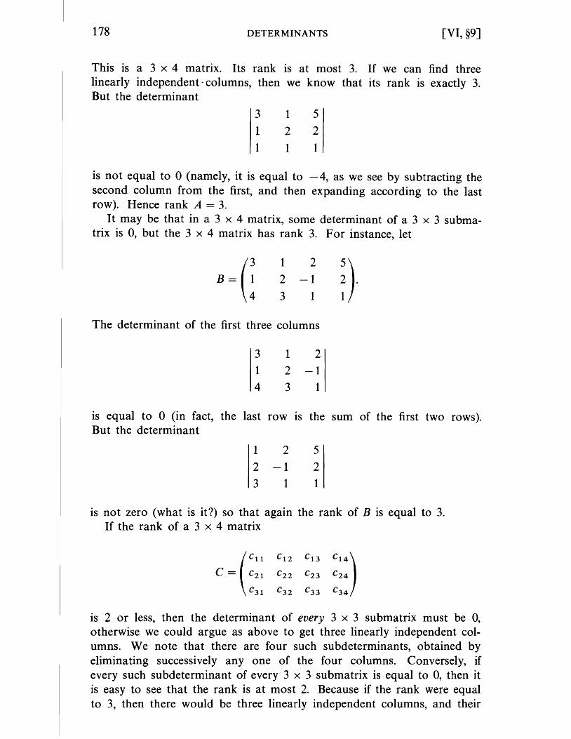
178 DETERMINANTS [VI, §9]
This is a 3 x 4 matrix. Its rank is at most 3. If we can find three linearly independent· columns, then we know that its rank is exactly 3. But the determinant
3
1
1
1
2
1
5
2
1
is not equal to ° (namely, it is equal to -4, as we see by subtracting the second column from the first, and then expanding according to the last row). Hence rank A = 3.
It may be that in a 3 x 4 matrix, some determinant of a 3 x 3 submatrix is 0, but the 3 x 4 matrix has rank 3. For instance, let
B=(! 1 2
2 -1
3 1
The determinant of the first three columns
3 1 2
1 2 -1
4 3 1
is equal to ° (in fact, the last row IS the But the determinant
125
2 -1 2 3 1 1
sum of the first two rows).
is not zero (what is it?) so that again the rank of B is equal to 3. If the rank of a 3 x 4 matrix
C l2 C l3
C22 C23
C32 C33
is 2 or less, then the determinant of every 3 x 3 submatrix must be 0, otherwise we could argue as above to get three linearly independent columns. We note that there are four such subdeterminants, obtained by eliminating successively anyone of the four columns. Conversely, if every such subdeterminant of every 3 x 3 submatrix is equal to 0, then it is easy to see that the rank is at most 2. Because if the rank were equal to 3, then there would be three linearly independent columns, and their
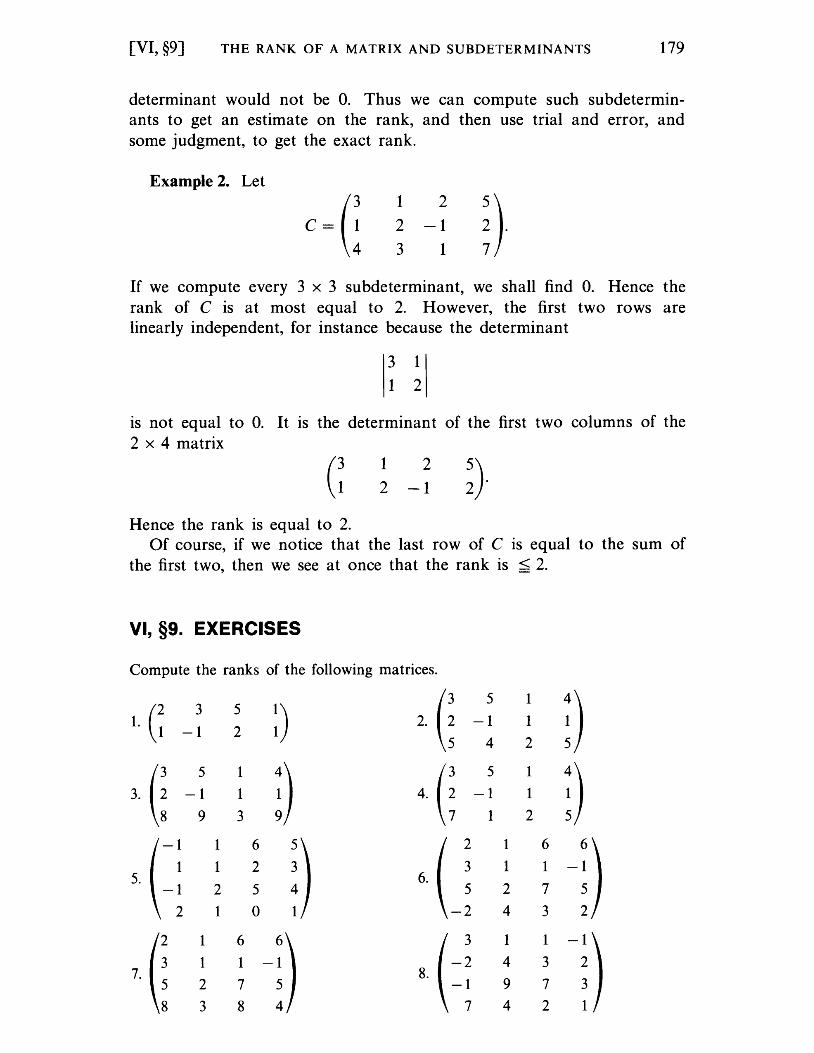
[VI, §9] THE RANK OF A MATRIX AND SUBDETERMINANTS 179
determinant would not be o. Thus we can compute such subdeterminants to get an estimate on the rank, and then use trial and error, and some judgment, to get the exact rank.
Example 2. Let
c = (! 1 2
2 -1
3 1
If we compute every 3 x 3 subdeterminant, we shall find o. Hence the rank of C is at most equal to 2. However, the first two rows are linearly independent, for instance because the determinant
3 1
1 2
is not equal to O. It is the determinant of the first two columns of the 2 x 4 matrix
Hence the rank is equal to 2.
1 2
2 -1
Of course, if we notice that the last row of C is equal to the sum of the first two, then we see at once that the rank is < 2.
VI, §9. EXERCISES
Compute the ranks of the following matrices.
~) 2. G 5 1
:) 1. (~ 3 5 -1 1
-1 2 4 2
3. G 5 1
n 4. G 5 1
D -1 1 -1 1
9 3 1 2
-1 1 6
~) 2 1 6
-~) 1 1 2 3 1 1 5. 6.
-1 2 5 5 2 7
2 1 0 -2 4 3
7. (;
1 6
-~) ( -~ 1 1
-~) 1 1 4 3 8.
9 2 7 -1 7
3 8 7 4 2
CHAPTER VII
Symmetric, Hermitian, and Unitary Operators
Let V be a finite dimensional vector space over the real or complex n urn bers, with a posi ti ve definite scalar product. Let
A: V -+ V
be a linear map. We shall study three important special cases of such maps, named in the title of this chapter. Such maps are also represented by matrices bearing the same names when a basis of V has been chosen.
In Chapter VIII we shall study such maps further and show that a basis can be chosen such that the maps are represented by diagonal matrices. This ties up with the theory of eigenvectors and eigenvalues.
VII, §1. SYMMETRIC OPERATORS
Throughout this section we let V be a finite dimensional vector space over a field K. We suppose that V has a fixed non-degenerate scalar product denoted by <v, w), for v, WE V.
The reader may take V = K n and may fix the scalar product to be the ordinary dot product
<x, Y) = tXY,
where X, Yare column vectors in Kn. However, in applications, it is not a good idea to fix such bases right away.
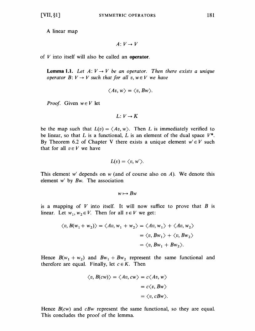
[VII, §1] SYMMETRIC OPERATORS 181
A linear map
A: V -+ V
of V into itself will also be called an operator.
Lemma 1.1. Let A: V -+ V be an operator. Then there exists a unique operator B: V -+ V such that for all v, WE V we have
<Av, W) = <v, Bw).
Proof. Given WE V let
L: V-+K
be the map such that L(v) = <Av, w). Then L is immediately verified to be linear, so that L is a functional, L is an element of the dual space V*. By Theorem 6.2 of Chapter V there exists a unique element w' E V such that for all v E V we have
L(v) = <v, w').
This element w' depends on w (and of course also on A). We denote this element w' by Bw. The association
W 1--+ Bw
IS a mapping of V into itself. It will now suffice to prove that B IS
linear. Let Wl' w2 E V. Then for all v E V we get:
<v, B(Wl + w2) = <Av, W l + w2) = <Av, wl ) + <Av, w2)
= <v, Bwl ) + <v, Bw2)
= <v, BWI + Bw2).
Hence B(Wl + w2) and BWl + BW2 represent the same functional and therefore are equal. Finally, let c E K. Then
<v, B(cw) = <Av, cw) = c<Av, w)
= c<v, Bw)
= <v, cBw).
Hence B(cw) and cBw represent the same functional, so they are equal. This concludes the proof of the lemma.
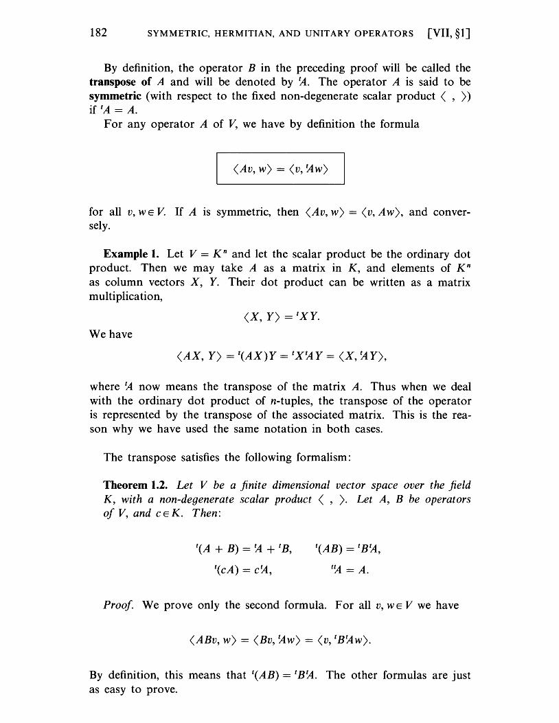
182 SYMMETRIC, HERMITIAN, AND UNITARY OPERATORS [VII, §1]
By definition, the operator B in the preceding proof will be called the transpose of A and will be denoted by~. The operator A is said to be symmetric (with respect to the fixed non-degenerate scalar product ( , ») if tA = A.
For any operator A of V, we have by definition the formula
(Av, w) = (v, ~w)
for all v, WE V. If A is symmetric, then (Av, w) = (v, Aw), and conversely.
Example 1. Let V = Kn and let the scalar product be the ordinary dot product. Then we may take A as a matrix in K, and elements of Kn as column vectors X, Y. Their dot product can be written as a matrix multiplication,
(X, Y) = tXY.
We have
(AX, Y) = t(AX)Y = tx~Y = (X, ~Y),
where ~ now means the transpose of the matrix A. Thus when we deal with the ordinary dot product of n-tuples, the transpose of the operator is represented by the transpose of the associated matrix. This is the reason why we have used the same notation in both cases.
The transpose satisfies the following formalism:
Theorem 1.2. Let V be a finite dimensional vector space over the field K, with a non-degenerate scalar product ( , ). Let A, B be operators of V, and c E K. Then:
t(A + B) = ~ + tB,
t(cA) = c~,
t(AB) = tB~,
t~ = A.
Proof. We prove only the second formula. For all v, WE V we have
(ABv, w) = (Bv, ~w) = (v, tB~w).
By definition, this means that t(AB) = tB~. The other formulas are just as easy to prove.
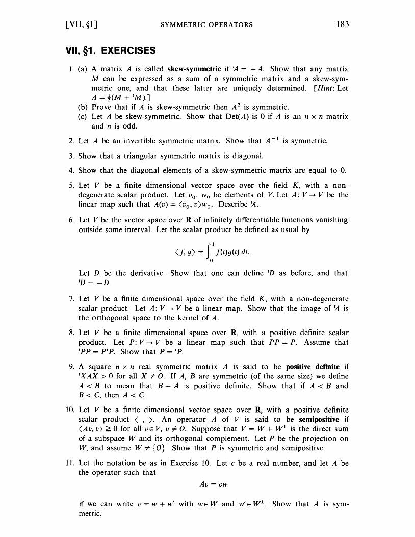
[VII, §1] SYMMETRIC OPERATORS 183
VII, §1. EXERCISES
1. (a) A matrix A is called skew-symmetric if ~ = - A. Show that any matrix M can be expressed as a sum of a symmetric matrix and a skew-symmetric one, and that these latter are uniquely determined. [Hint: Let A = t(M + 'M).]
(b) Prove that if A is skew-symmetric then A2 is symmetric. (c) Let A be skew-symmetric. Show that Det(A) is 0 if A is an n x n matrix
and n is odd.
2. Let A be an invertible symmetric matrix. Show that A-I is symmetric.
3. Show that a triangular symmetric matrix is diagonal.
4. Show that the diagonal elements of a skew-symmetric matrix are equal to o.
5. Let V be a finite dimensional vector space over the field K, with a nondegenerate scalar product. Let vo, Wo be elements of V. Let A: V ~ V be the linear map such that A(v) = (vo, v)wo. Describe~.
6. Let V be the vector space over R of infinitely differentiable functions vanishing outside some interval. Let the scalar product be defined as usual by
<f, g) = f 1 f(t)g(t) dt. o
Let D be the derivative. Show that one can define tD as before, and that tD= -D.
7. Let V be a finite dimensional space over the field K, with a non-degenerate scalar product. Let A: V ~ V be a linear map. Show that the image of ~ is the orthogonal space to the kernel of A.
8. Let V be a finite dimensional space over R, with a positive definite scalar product. Let P: V ~ V be a linear map such that PP = P. Assume that tpp = ptP. Show that P = tP.
9. A square n x n real symmetric matrix A is said to be positive definite if 'X AX > 0 for all X =I o. If A, B are symmetric (of the same size) we define A < B to mean that B - A is positive definite. Show that if A < Band B < C, then A < C.
10. Let V be a finite dimensional vector space over R, with a posItIve definite scalar product ( ,). An operator A of V is said to be semipositive if (Av, v) ~ 0 for all VE V, v =I o. Suppose that V = W + Wl. is the direct sum of a subspace Wand its orthogonal complement. Let P be the projection on W, and assume W i= {O}. Show that P is symmetric and semipositive.
11. Let the notation be as in Exercise 10. Let c be a real number, and let A be the operator such that
Av = cw
if we can write v = w + w' with WE Wand w' E Wl.. Show that A is symmetric.
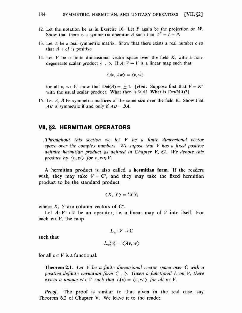
184 SYMMETRIC, HERMITIAN, AND UNITARY OPERATORS [VII, §2]
12. Let the notation be as in Exercise 10. Let P again be the projection on W. Show that there is a symmetric operator A such that A 2 = I + P.
13. Let A be a real symmetric matrix. Show that there exists a real number c so that A + cI is positive.
14. Let V be a finite dimensional vector space over the field K, with a nondegenerate scalar product < , ). If A: V ~ V is a linear map such that
<Av, Aw) = <v, w)
for all v, WE V, show that Det(A) = ± 1. [Hint: Suppose first that V = K n
with the usual scalar product. What then is ~A? What is Det(~A)?]
15. Let A, B be symmetric matrices of the same size over the field K. Show that AB is symmetric if and only if AB = BA.
VII, §2. HERMITIAN OPERATORS
. Throughout this section we let V be a finite dimensional vector space over the complex numbers. We supose that V has a fixed positive definite hermitian product as defined in Chapter V, §2. We denote this product by <v, w) for v, WE V.
A hermitian product is also called a hermitian form. If the readers wish, they may take V = en, and they may take the fixed hermitian product to be the standard product
<x, Y) = tX¥",
where X, Yare column vectors of en. Let A: V --. V be an operator, i.e. a linear map of V into itself. For
each WE V, the map
such that
for all v E V is a functional.
Theorem 2.1. Let V be a finite dimensional vector space over C with a positive definite hermitian form < , ). Given a functional L on V, there exists a unique w' E V such that L(v) = <v, w') for all v E V.
Proof. The proof is similar to that given in the real case, say Theorem 6.2 of Chapter V. We leave it to the reader.
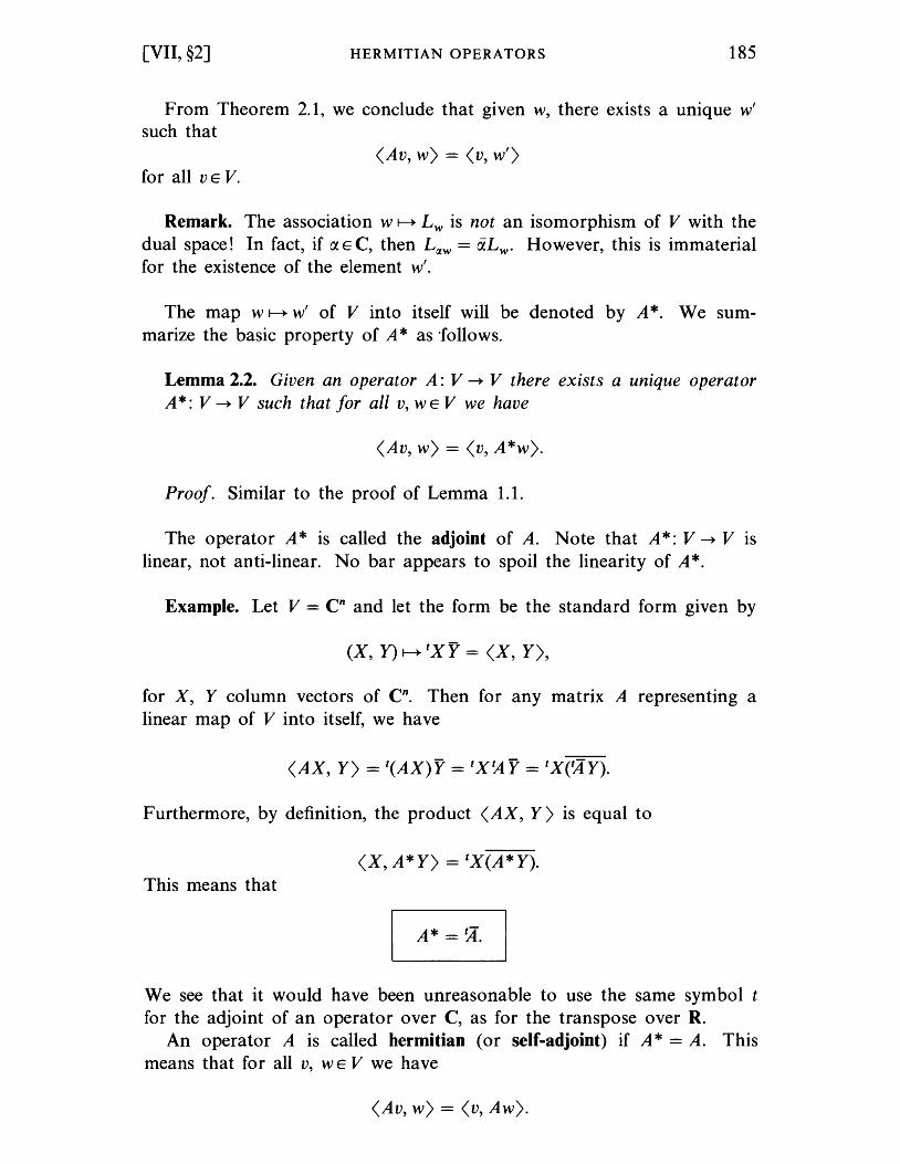
[VII, §2] HERMITIAN OPERATORS 185
From Theorem 2.1, we conclude that given w, there exists a unique w' such that
<Av, w) = <v, w') for all VE V.
Remark. The association w 1--+ Lw is not an isomorphism of V with the dual space! In fact, if rJ., E C, then L(lW = aLw' However, this is immaterial for the existence of the element w'.
The map w 1--+ w' of V into itself will be denoted by A*. We summarize the basic property of A * as 'follows.
Lemma 2.2. Given an operator A: V ---+ V there exists a unique operator A *: V ---+ V such that for all v, WE V we have
<Av, w) = <v, A*w).
Proof. Similar to the proof of Lemma 1.1.
The operator A * is called the adjoint of A. Note that A *: V ---+ V is linear, not anti-linear. No bar appears to spoil the linearity of A *.
Example. Let V = cn and let the form be the standard form given by
for X, Y column vectors of cn. Then for any matrix A representing a linear map of V into itself, we have
Furthermore, by definition, the product <AX, Y) is equal to
<X, A*Y) = tX(A*Y). This means that
A* =~.
We see that it would have been unreasonable to use the same symbol t for the adjoint of an operator over C, as for the transpose over R.
An operator A is called hermitian (or self-adjoint) if A * = A. This means that for all v, WE V we have
<Av, w) = <v, Aw).
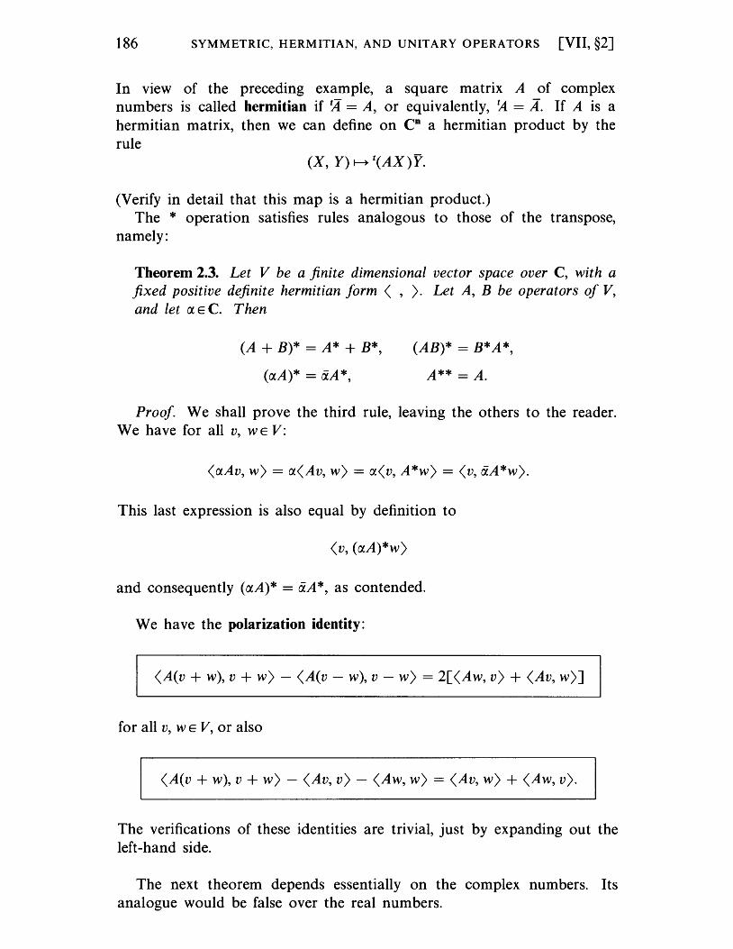
186 SYMMETRIC, HERMITIAN, AND UNITARY OPERATORS [VII, §2]
In view of the preceding example, a square matrix A of complex numbers is called hermitian if ~ = A, or equivalently, ~ = A. If A is a hermitian matrix, then we can define on Cn a hermitian product by the rule
(Verify in detail that this map is a hermitian product.) The * operation satisfies rules analogous to those of the transpose,
namely:
Theorem 2.3. Let V be a finite dimensional vector space over C, with a fixed positive definite hermitian form ( , ). Let A, B be operators of V, and let a E C. Then
(A + B)* = A* + B*,
(aA)* = ~A*,
(AB)* = B*A*,
A** = A.
Proof. We shall prove the third rule, leaving the others to the reader. We have for all v, WE V:
(aAv, w) = a(Av, w) = a(v, A*w) = (v, ~A*w).
This last expression is also equal by definition to
(v, (aA)*w)
and consequently (aA)* = ~A*, as contended.
We have the polarization identity:
(A(v + w), v + w) - (A(v - w), v - w) = 2[(Aw, v) + (Av, w)]
for all v, WE V, or also
(A(v + w), v + w) - (Av, v) - (Aw, w) = (Av, w) + (Aw, v).
The verifications of these identities are trivial, just by expanding out the left -hand side.
The next theorem depends essentially on the complex numbers. Its analogue would be false over the real numbers.
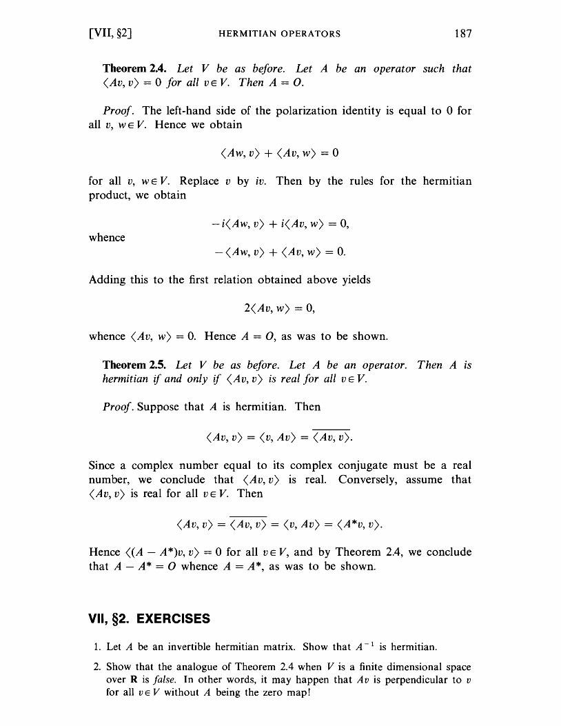
[VII, §2] HERMITIAN OPERATORS 187
Theorem 2.4. Let V be as before. Let A be an operator such that <Av, v) = 0 for all VE V. Then A = o.
Proof. The left-hand side of the polarization identity is equal to 0 for all v, WE V. Hence we obtain
<Aw, v) + <Av, w) = 0
for all v, WE V. Replace v by iv. Then by the rules for the hermitian product, we obtain
-i<Aw, v) + i<Av, w) = 0, whence
-<Aw, v) + <Av, w) = o.
Adding this to the first relation obtained above yields
2<Av, w) = 0,
whence <Av, w) = O. Hence A = 0, as was to be shown.
Theorem 2.5. Let V be as before. Let A be an operator. Then A is hermitian if and only if < Av, v) is real for all v E V.
Proof. Suppose that A is hermitian. Then
<Av, v) = <v, Av) = <Av, v).
Since a complex number equal to its complex conjugate must be a real number, we conclude that <Av, v) is real. Conversely, assume that <Av, v) is real for all v E V. Then
<Av, v) = <Av, v) = <v, Av) = <A*v, v).
Hence «A - A*)v, v) = 0 for all VE V, and by Theorem 2.4, we conclude that A - A* = 0 whence A = A*, as was to be shown.
VII, §2. EXERCISES
1. Let A be an invertible hermitian matrix. Show that A-I is hermitian.
2. Show that the analogue of Theorem 2.4 when V is a finite dimensional space over R is false. In other words, it may happen that Av is perpendicular to v for all v E V without A being the zero map!
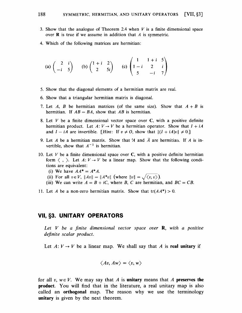
188 SYMMETRIC, HERMITIAN, AND UNITARY OPERATORS [VII, §3]
3. Show that the analogue of Theorem 2.4 when V is a finite dimensional space over R is true if we assume in addition that A is symmetric.
4. Which of the following matrices are hermitian:
(a) (_~ ~) (1 + i 2)
(b) 2 5i
1 + i 2
-i
5. Show that the diagonal elements of a hermitian matrix are real.
6. Show that a triangular hermitian matrix is diagonal.
7. Let A, B be hermitian matrices (of the same size). Show that A + B is hermitian. If AB = BA, show that AB is hermitian.
8. Let V be a finite dimensional vector space over C, with a positive definite hermitian product. Let A: V ~ V be a hermitian operator. Show that 1 + iA and 1 - iA are invertible. [Hint: If v * 0, show that 11(1 + iA)vll * 0.]
9. Let A be a hermitian matrix. Show that ~ and A are hermitian. If A is invertible, show that A - 1 is hermitian.
10. Let V be a finite dimensional space over C, with a positive definite hermitian form < , ). Let A: V ~ V be a linear map. Show that the following conditions are equivalent:
(i) We have AA* = A* A. (ii) For all VE V, IIAvl1 = IIA*vll (where Ilvll = j(;,0).
(iii) We can write A = B + iC, where B, C are hermitian, and BC = CB.
11. Let A be a non-zero hermitian matrix. Show that tr(AA *) > O.
VII, §3. UNITARY OPERATORS
Let V be a finite dimensional vector space over R, with a positive definite scalar product.
Let A: V -+ V be a linear map. We shall say that A is real unitary if
(Av, Aw) = (v, w)
for all v, WE V. We may say that A is unitary means that A preserves the product. You will find that in the literature, a real unitary map is also called an orthogonal map. The reason why we use the terminology unitary is given by the next theorem.
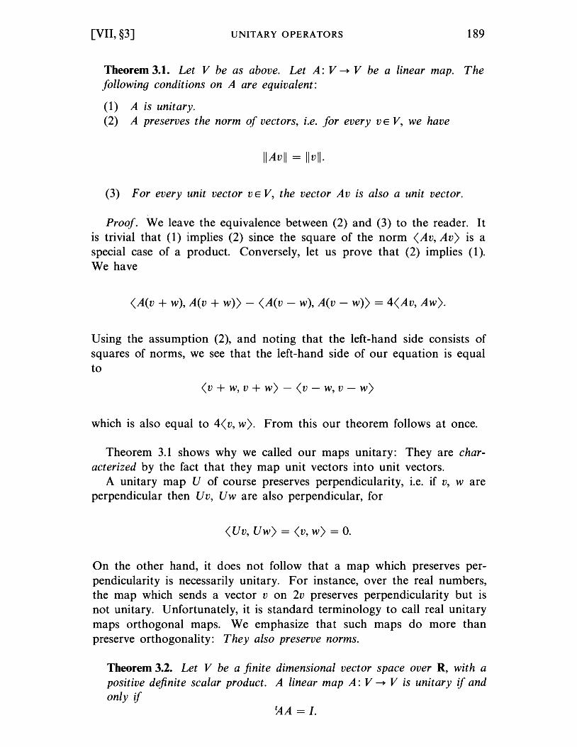
[VII, §3] UNITARY OPERATORS 189
Theorem 3.1. Let V be as above. Let A: V ---+ V be a linear map. The following conditions on A are equivalent:
(1) A is unitary. (2) A preserves the norm of vectors, i.e. for every v E V, we have
IIAvl1 = Ilvll·
(3) F or every unit vector v E V, the vector Av is also a unit vector.
Proof. We leave the equivalence between (2) and (3) to the reader. It is trivial that (1) implies (2) since the square of the norm <Av, Av) is a special case of a product. Conversely, let us prove that (2) implies (1). We have
<A(v + w), A(v + w) - <A(v - w), A(v - w) = 4<Av, Aw).
Using the assumption (2), and noting that the left-hand side consists of squares of norms, we see that the left-hand side of our equation is equal to
<v + w, v + w) - <v - w, v - w)
which is also equal to 4<v, w). From this our theorem follows at once.
Theorem 3.1 shows why we called our maps unitary: They are characterized by the fact that they map unit vectors into unit vectors.
A unitary map U of course preserves perpendicularity, i.e. if v, ware perpendicular then Uv, Uw are also perpendicular, for
<Uv, Uw) = <v, w) = O.
On the other hand, it does not follow that a map which preserves perpendicularity is necessarily unitary. For instance, over the real numbers, the map which sends a vector v on 2v preserves perpendicularity but is not unitary. Unfortunately, it is standard terminology to call real unitary maps orthogonal maps. We emphasize that such maps do more than preserve orthogonality: They also preserve norms.
Theorem 3.2. Let V be a finite dimensional vector space over R, with a positive definite scalar product. A linear map A: V ---+ V is unitary if and only if
~A =1.
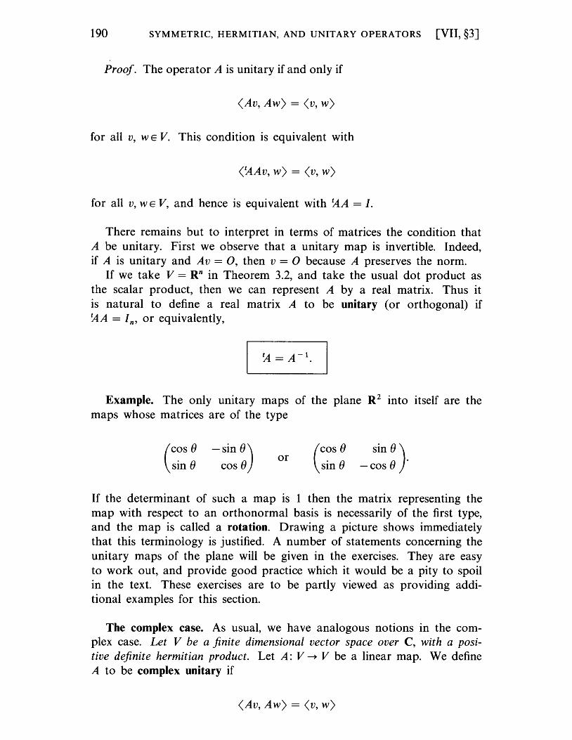
190 SYMMETRIC, HERMITIAN, AND UNITARY OPERATORS [VII, §3]
Proof. The operator A is unitary if and only if
(Av, Aw) = (v, w)
for all v, WE V. This condition is equivalent with
(~Av, w) = (v, w)
for all v, WE V, and hence is equivalent with ~A = I.
There remains but to interpret in terms of matrices the condition that A be unitary. First we observe that a unitary map is invertible. Indeed, if A is unitary and Av = 0, then v = 0 because A preserves the norm.
If we take V = Rn in Theorem 3.2, and take the usual dot product as the scalar product, then we can represent A by a real matrix. Thus it is natural to define a real matrix A to be unitary (or orthogonal) if ~A = In' or equivalently,
Example. The only unitary maps of the plane R2 into itself are the maps whose matrices are of the type
(
COS ()
sin () -sin ())
cos () or
(
COS ()
sin () sin ())
-cos () .
If the determinant of such a map is 1 then the matrix representing the map with respect to an orthonormal basis is necessarily of the first type, and the map is called a rotation. Drawing a picture shows immediately that this terminology is justified. A number of statements concerning the unitary maps of the plane will be given in the exercises. They are easy to work out, and provide good practice which it would be a pity to spoil in the text. These exercises are to be partly viewed as providing additional examples for this section.
The complex case. As usual, we have analogous notions in the complex case. Let V be a finite dimensional vector space over C, with a positive definite hermitian product. Let A: V --+ V be a linear map. We define A to be complex unitary if
(Av, Aw) = (v, w)
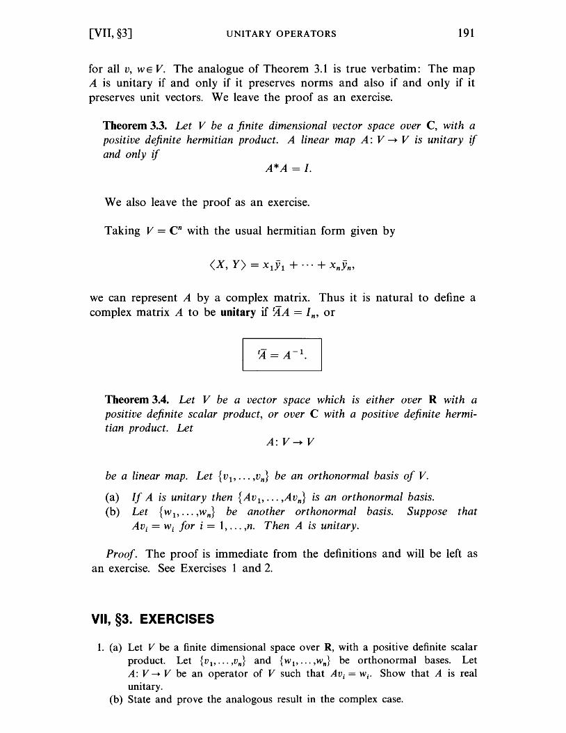
[VII, §3] UNITARY OPERATORS 191
for all v, WE V. The analogue of Theorem 3.1 is true verbatim: The map A is unitary if and only if it preserves norms and also if and only if it preserves unit vectors. We leave the proof as an exercise.
Theorem 3.3. Let V be a finite dimensional vector space over C, with a positive definite hermitian product. A linear map A: V --+ V is unitary if and only if
A*A = I.
We also leave the proof as an exercise.
Taking V = cn with the usual hermitian form given by
we can represent A by a complex matrix. Thus it is natural to define a complex matrix A to be unitary if ~A = In' or
Theorem 3.4. Let V be a vector space which is either over R with a positive definite scalar product, or over C with a positive definite hermitian product. Let
A: V--+ V
be a linear map. Let {v I' ... ,vn} be an orthonormal basis of v. (a) If A is unitary then {Av l , ... ,Avn } is an orthonormal basis. (b) Let {WI' ... ,wn} be another orthonormal basis. Suppose that
AVi = Wi for i = 1, ... ,no Then A is unitary.
Proof. The proof is immediate from the definitions and will be left as an exercise. See Exercises 1 and 2.
VII, §3. EXERCISES
1. (a) Let V be a finite dimensional space over R, with a positive definite scalar product. Let {VI' ... ,vn } and {WI' ... ,wn } be orthonormal bases. Let A: V ---+ V be an operator of V such that AVi = Wi. Show that A is real unitary.
(b) State and prove the analogous result in the complex case.
192 SYMMETRIC, HERMITIAN, AND UNITARY OPERATORS [VII, §3]
2. Let V be as in Exercise 1. Let {v l' ... ,vn } be an orthonormal basis of V. Let A be a unitary operator of V. Show that {Av l' ... ,Avn} is an orthonormal basis.
3. Let A be a real unitary matrix. (a) Show that ~ is unitary. (b) Show that A - 1 exists and is unitary. (c) If B is real unitary, show that AB is unitary, and that B- 1 AB is unitary.
4. Let A be a complex unitary matrix. (a) Show that ~ is unitary (b) Show that A - 1 exists and is unitary. (c) If B is complex unitary, show that AB is unitary, and that B- 1 AB is
unitary.
5. (a) Let V be a finite dimensional space over R, with a positive definite scalar product, and let {v 1, ••• ,vn } = (!A and {W l' ... ,Wn } = (!A' be orthonormal bases of V. Show that the matrix M:, (id) is real unitary. [Hint: Use < Wi' Wi) = 1 and <Wi' Wj ) = 0 if i #- j, as well as the expression Wi = L aijvj, for some aijER.]
(b) Let F: V --+ V be such that F(v i ) = Wi for all i. Show that M:, (F) is unitary.
6. Show that the absolute value of the determinant of a real unitary matrix is equal to 1. Conclude that if A is real unitary, then Det(A) = 1 or -1.
7. If A is a complex square matrix, show that Det(A) = Det(A). Conclude that the absolute value of the determinant of a complex unitary matrix is equal to 1.
8. Let A be a diagonal real unitary matrix. Show that the diagonal elements of A are equal to 1 or -1.
9. Let A be a diagonal complex unitary matrix. Show that each diagonal element has absolute value 1, and hence is of type eiO
, with real B.
The following exercises describe various properties of real unitary maps of the plane R2.
10. Let V be a 2-dimensional vector space over R, with a positive definite scalar product, and let A be a real unitary map of V into itself. Let {Vi' V2 } and {W1' w2 } be orthonormal bases of v such that AVi = Wi for i = 1, 2. Let a, b, c, d be real numbers such that
Show that a2 + b2 = 1, c2 + d 2 = 1, ac + bd = 0, a2 = d 2 and c2 = b2•
11. Show that the determinant ad - bc is equal to 1 or - 1. (Show that its square is equal to 1.)
[VII, §3] UNITARY OPERATORS 193
12. Define a rotation of V to be a real unitary map A of V whose determinant is 1. Show that the matrix of A relative to an orthogonal basis of V is of type
for some real numbers a, b such that a2 + b2 = 1. Also prove the converse, that any linear map of V into itself represented by such a matrix on an orthogonal basis is unitary, and has determinant 1. Using calculus, one can then conclude that there exist a number e such that a = cos e and b = sin e.
13. Show that there exists a complex unitary matrix U such that, if
A = (COS e sin e
then U-lAU = B.
-sin e) cos e and
14. Let V = C be viewed as a vector space of dimension 2 over R. Let lJ, E C, and let La: C --+ C be the map z ~ lJ,z. Show that La is an R-linear map of V into itself. For which complex numbers lJ, is La a unitary map with respect to the scalar product <z, w) = Re(zw)? What is the matrix of La with respect to the basis {I, i} of Cover R?
CHAPTER VIII
Eigenvectors and Eigenvalues
This chapter gives the basic elementary properties of eigenvectors and eigenvalues. We get an application of determinants in computing the characteristic polynomial. In §3, we also get an elegant mixture of calculus and linear algebra by relating eigenvectors with the problem of finding the maximum and minimum of a quadratic function on the sphere. Most students taking linear algebra will have had some calculus, but the proof using complex numbers instead of the maximum principle can be used to get real eigenvalues of a symmetric matrix if the calculus has to be avoided. Basic properties of the complex numbers will be recalled in an appendix.
VIII, §1. EIGENVECTORS AND EIGENVALUES
Let V ee a vector space and let
A: V--+ V
be a linear map of V into itself. An element v E V is called an eigenvector of A if there exists a number A such that Av = AV. If v =1= 0 then A is uniquely determined, because Al v = A2 v implies Al = A2. In this case, we say that A is an eigenvalue of A belonging to the eigenvector v. We also say that v is an eigenvector with the eigenvalue A. Instead of eigenvector and eigenvalue, one also uses the terms characteristic vector and characteristic value.
If A is a square n x n matrix then an eigenvector of A is by definition an eigenvector of the linear map of K n into itself represented by this
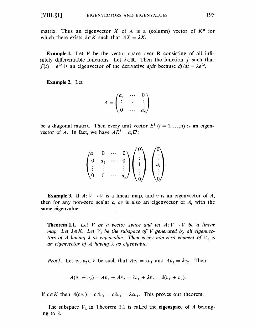
[VIII, §1] EIGENVECTORS AND EIGENVALUES 195
matrix. Thus an eigenvector X of A is a (column) vector of K n for which there exists A E K such that AX = AX.
Example 1. Let V be the vector space over R consisting of all infinitely differentiable functions. Let A E R. Then the function f such that f(t) = e;'t is an eigenvector of the derivative d/dt because df/dt = Ae;'t.
Example 2. Let
be a diagonal matrix. Then every unit vector Ei (i = 1, ... ,n) is an eigenvector of A. In fact, we have AEi = aiEi:
0 0 a l 0 0
0 a2 0 1 -
0 0 an 0
Example 3. If A: V -+ V is a linear map, and v is an eigenvector of A, then for any non-zero scalar c, cv is also an eigenvector of A, with the same eigenvalue.
Theorem 1.1. Let V be a vector space and let A: V -+ V be a linear map. Let A E K. Let V;. be the subspace of V generated by all eigenvectors of A having A as eigenvalue. Then every non-zero element of V;. is an eigenvector of A having A as eigenvalue.
Proof. Let VI' V2 E V be such that AVI = AV I and AV2 = AV2. Then
If CEK then A(cv l ) = CAVI = CAV I = ACV I. This proves our theorem.
The subspace V;. in Theorem 1.1 is called the eigenspace of A belonging to A.
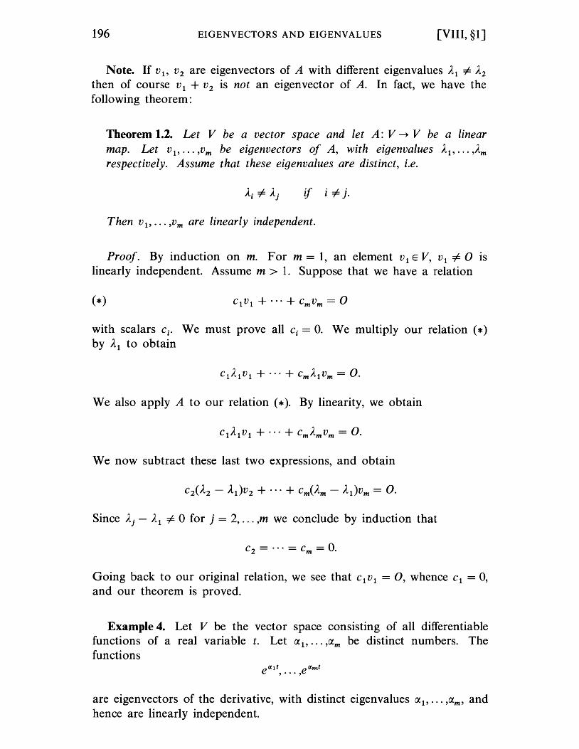
196 EIGENVECTORS AND EIGENVALUES [VIII, §1]
Note. If vl , V2 are eigenvectors of A with different eigenvalues Al =1= A2
then of course V l + V2 is not an eigenvector of A. In fact, we have the following theorem:
Theorem 1.2. Let V be a vector space and let A: V --+ V be a linear map. Let v l , ... ,Vm be eigenvectors of A, with eigenvalues Al , ... ,Am respectively. Assume that these eigenvalues are distinct, i.e.
if i =1= j.
Then v l , ... ,Vm are linearly independent.
Proof. By induction on m. For m = 1, an element V l E V, V l =1= 0 IS
linearly independent. Assume m > 1. Suppose that we have a relation
with scalars ci • We must prove all Ci = o. We multiply our relation (*) by A 1 to obtain
We also apply A to our relation (*). By linearity, we obtain
We now subtract these last two expressions, and obtain
Since Aj - Al =1= 0 for j = 2, ... ,m we conclude by induction that
Going back to our original relation, we see that C1V l = 0, whence C l = 0, and our theorem is proved.
Example 4. Let V be the vector space consisting of all differentiable functions of a real variable t. Let ct l , ... ,ctm be distinct numbers. The functions
are eigenvectors of the derivative, with distinct eigenvalues ct l , ... ,ctm , and hence are linearly independent.
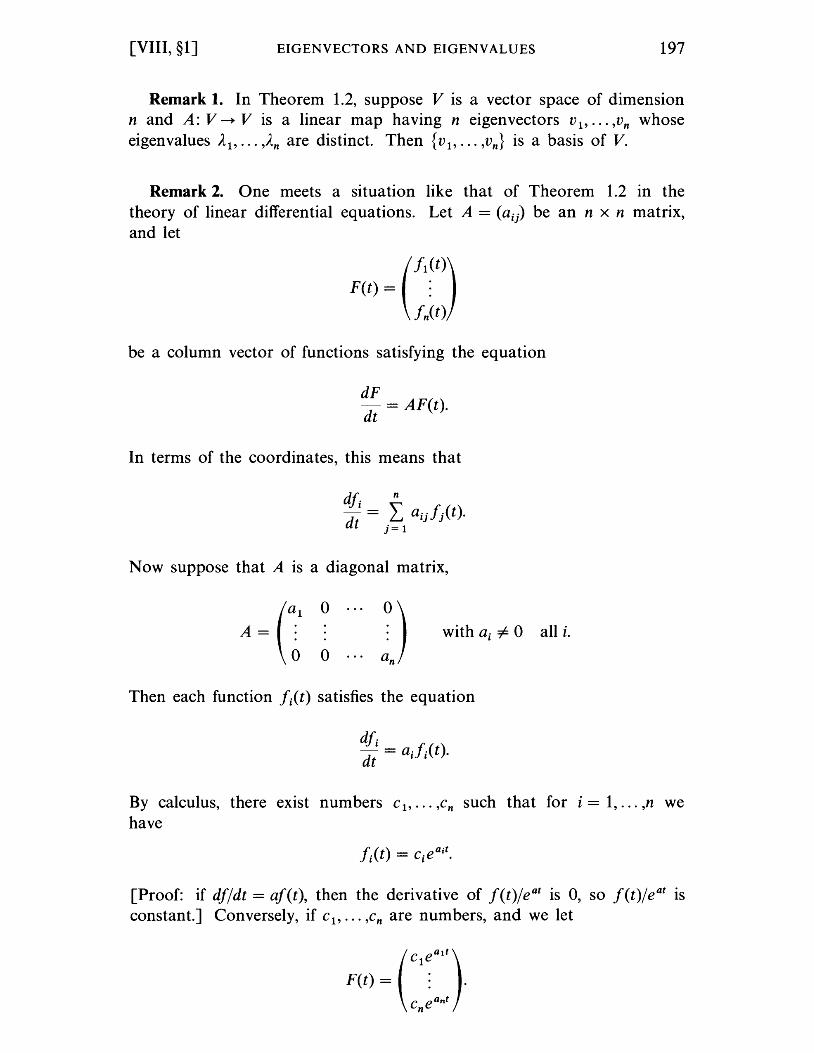
[VIII, §1] EIGENVECTORS AND EIGENVALUES 197
Remark 1. In Theorem 1.2, suppose V is a vector space of dimension n and A: V -+ V is a linear map having n eigenvectors V 1, ••• ,Vn whose eigenvalues A1 , ••• ,An are distinct. Then {V 1 , ••• ,Vn} is a basis of V.
Remark 2. One meets a situation like that of Theorem 1.2 In the theory of linear differential equations. Let A = (aij) be an n x n matrix, and let
F(t) = : (
f1 (t))
fn(t)
be a column vector of functions satisfying the equation
dF dt = AF(t).
In terms of the coordinates, this means that
Now suppose that A is a diagonal matrix,
A = (: ! ::: I) with ai -1= 0 all i.
Then each function fi(t) satisfies the equation
By calculus, there exist numbers C b ... 'Cn such that for i = 1, ... ,n we have
[Proof: if df/dt = af(t), then the derivative of f(t)/e at is 0, so f(t)/e at is constant.] Conversely, if C 1, ••• 'Cn are numbers, and we let
(
c ealt) F(t) = 1 : .
C eant n
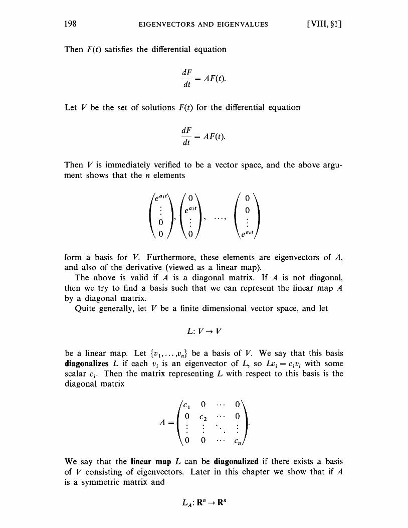
198 EIGENVECTORS AND EIGENVALUES [VIII, §1]
Then F(t) satisfies the differential equation
dF dt = AF(t).
Let V be the set of solutions F(t) for the differential equation
dF at = AF(t).
Then V is immediately verified to be a vector space, and the above argument shows that the n elements
... ,
form a basis for V. Furthermore, these elements are eigenvectors of A, and also of the derivative (viewed as a linear map).
The above is valid if A is a diagonal matrix. If A is not diagonal, then we try to find a basis such that we can represent the linear map A by a diagonal matrix.
Quite generally, let V be a finite dimensional vector space, and let
L: V -+ V
be a linear map. Let {v l , ..• ,vn } be a basis of V. We say that this basis diagonalizes L if each Vi is an eigenvector of L, so LVi = CiVi with some scalar Ci • Then the matrix representing L with respect to this basis is the diagonal matrix
o C2 o A=
We say that the linear map L can be diagonalized if there exists a basis of V consisting of eigenvectors. Later in this chapter we show that if A is a symmetric matrix and
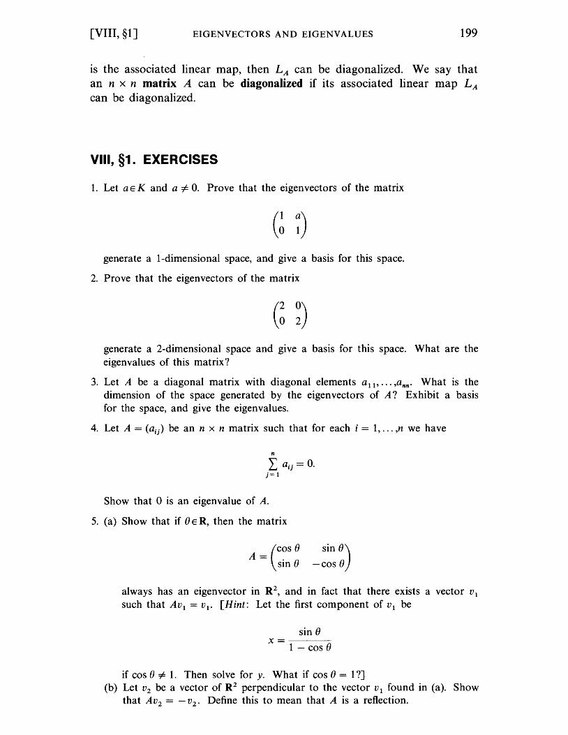
[VIII, §1] EIGENVECTORS AND EIGENVALUES 199
is the associated linear map, then LA can be diagonalized. We say that an n x n matrix A can be diagonalized if its associated linear map LA can be diagonalized.
VIII, §1. EXERCISES
1. Let a E K and a #- o. Prove that the eigenvectors of the matrix
generate a I-dimensional space, and give a basis for this space.
2. Prove that the eigenvectors of the matrix
generate a 2-dimensional space and give a basis for this space. What are the eigenvalues of this matrix?
3. Let A be a diagonal matrix with diagonal elements all' ... ,ann. What is the dimension of the space generated by the eigenvectors of A? Exhibit a basis for the space, and give the eigenvalues.
4. Let A = (aij ) be an n x n matrix such that for each i = 1, ... ,n we have
n
L aij = O. j= 1
Show that 0 is an eigenvalue of A.
5. (a) Show that if 8ER, then the matrix
A = (COS 8 sin 8
sin 8) -cos 8
always has an eigenvector in R2, and in fact that there exists a vector V l
such that AVl = Vl. [Hint: Let the first component of V l be
sin 8 x=----
1 - cos 8
if cos 8 #- 1. Then solve for y. What if cos 8 = I?] (b) Let V2 be a vector of R2 perpendicular to the vector V l found in (a). Show
that AV2 = - v2 . Define this to mean that A is a reflection.
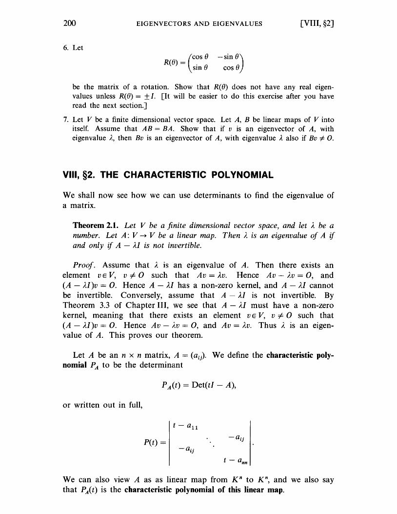
200
6. Let
EIGENVECTORS AND EIGENVALUES
(
COS 0 R(O) = . 0
SIn
- sin 0) cos 0
[VIII, §2]
be the matrix of a rotation. Show that R(O) does not have any real eigenval ues unless R( 0) = ± I. [I t will be easier to do this exercise after you have read the next section.]
7. Let V be a finite dimensional vector space. Let A, B be linear maps of V into itself. Assume that AB = BA. Show that if v is an eigenvector of A, with eigenvalue A, then Bv is an eigenvector of A, with eigenvalue A also if Bv #- O.
VIII, §2. THE CHARACTERISTIC POLYNOMIAL
We shall now see how we can use determinants to find the eigenvalue of a matrix.
Theorem 2.1. Let V be a finite dimensional vector space, and let A be a number. Let A: V ~ V be a linear map. Then A is an eigenvalue of A if and only if A - AI is not invertible.
Proof. Assume that A is an eigenvalue of A. Then there exists an element v E V, v =I- 0 such that Av = Av. Hence Av - AV = 0, and (A - AI)v = O. Hence A - AI has a non-zero kernel, and A - AI cannot be invertible. Conversely, assume that A - AI is not invertible. By Theorem 3.3 of Chapter III, we see that A - AI must have a non-zero kernel, meaning that there exists an element v E V, v =I- 0 such that (A - AI)v = O. Hence Av - AV = 0, and Av = Av. Thus A is an eigenvalue of A. This proves our theorem.
Let A be an n x n matrix, A = (aij). We define the characteristic polynomial PA to be the determinant
PA(t) = Det(tI - A),
or written out in full,
P(t) =
We can also view A as as linear map from K n to K n, and we also say
that PA(t) is the characteristic polynomial of this linear map.
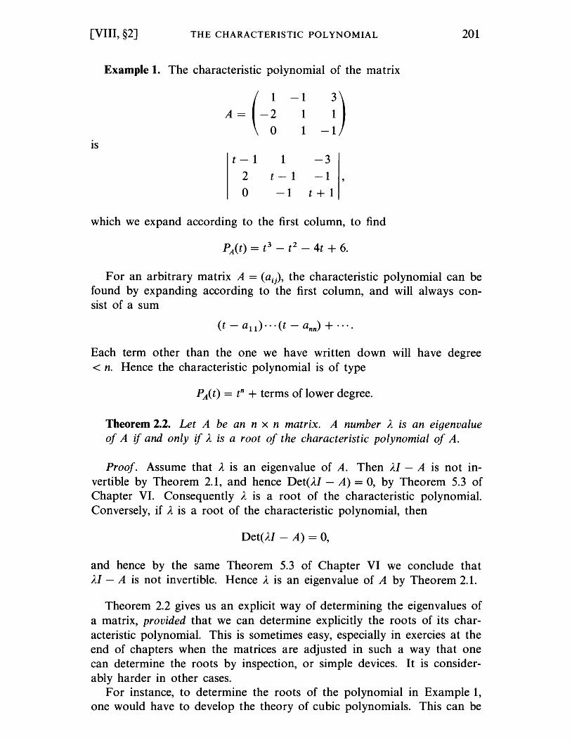
[VIII, §2] THE CHARACTERISTIC POLYNOMIAL 201
Example 1. The characteristic polynomial of the matrix
A = (-~ -1
-:) 1 1
IS
t - 1 1 -3 2 t - 1 -1
0 -1 t + 1
which we expand according to the first column, to find
For an arbitrary matrix A = (aij), the characteristic polynomial can be found by expanding according to the first column, and will always consist of a sum
Each term other than the one we have written down will have degree < n. Hence the characteristic polynomial is of type
PA(t) = tn + terms of lower degree.
Theorem 2.2. Let A be an n x n matrix. A number A is an eigenvalue of A if and only if A is a root of the characteristic polynomial of A.
Proof. Assume that A is an eigenvalue of A. Then AI - A is not invertible by Theorem 2.1, and hence Det(AI - A) = 0, by Theorem 5.3 of Chapter VI. Consequently A is a root of the characteristic polynomial. Conversely, if A is a root of the characteristic polynomial, then
Det(AI - A) = 0,
and hence by the same Theorem 5.3 of Chapter VI we conclude that AI - A is not invertible. Hence A is an eigenvalue of A by Theorem 2.1.
Theorem 2.2 gives us an explicit way of determining the eigenvalues of a matrix, provided that we can determine explicitly the roots of its characteristic polynomial. This is sometimes easy, especially in exercies at the end of chapters when the matrices are adjusted in such a way that one can determine the roots by inspection, or simple devices. It is considerably harder in other cases.
For instance, to determine the roots of the polynomial in Example 1, one would have to develop the theory of cubic polynomials. This can be
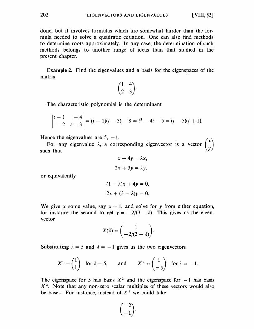
202 EIGENVECTORS AND EIGENVALUES [VIII, §2]
done, but it involves formulas which are somewhat harder than the formula needed to solve a quadratic equation. One can also find methods to determine roots approximately. In any case, the determination of such methods belongs to another range of ideas than that studied in the present chapter.
Example 2. Find the eigenvalues and a basis for the eigenspaces of the matrix
The characteristic polynomial is the determinant
t - 1 - 4 = (t - 1)(t - 3) - 8 = t 2
- 4t - 5 = (t - 5)(t + 1). - 2 t - 3
Hence the eigenvalues are 5, - 1. For any eigenvalue A, a corresponding eigenvector is a vector (;)
such that
or equivalently
x + 4y = AX,
2x + 3y = Ay,
(1 - A)X + 4y = 0,
2x + (3 - A)y = O.
We give X some value, say X = 1, and solve for y from either equation, for instance the second to get y = - 2/(3 - A). This gives us the eigenvector
X(A.) = ( -2/(~ - A.)}
Substituting A = 5 and A = -1 gives us the two eigenvectors
and
The eigenspace for 5 has basis Xl and the eigenspace for -1 has basis X2. Note that any non-zero scalar multiples of these vectors would also be bases. For instance, instead of X 2 we could take
(-~)
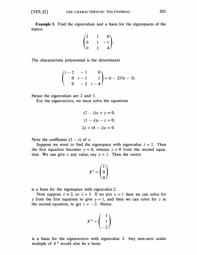
[VIII, §2] THE CHARACTERISTIC POLYNOMIAL 203
Example 3. Find the eigenvalues and a basis for the eigenspaces of the matrix
(~ 1
1
2 -!)
The characteristic polynomial is the determinant
(
t - 2 - 1 0) o t - 1 1 = (t - 2)2(t - 3).
o -2 t-4
Hence the eigenvalues are 2 and 3. For the eigenvectors, we must solve the equations
(2 - A)X + Y = 0,
(1 - A)Y - Z = 0,
2y+(4-A)Z=0.
Note the coefficient (2 - A) of x. Suppose we want to find the eigenspace with eigenvalue A = 2. Then
the first equation becomes y = 0, whence Z = 0 from the second equation. We can give x any value, say x = 1. Then the vector
is a basis for the eigenspace with eigenvalue 2. Now suppose A =1= 2, so A = 3. If we put x = 1 then we can solve for
y from the first equation to give y = 1, and then we can solve for Z in the second equation, to get z = - 2. Hence
is a basis for the eigenvectors with eigenvalue 3. Any non-zero scalar multiple of X 2 would also be a basis.
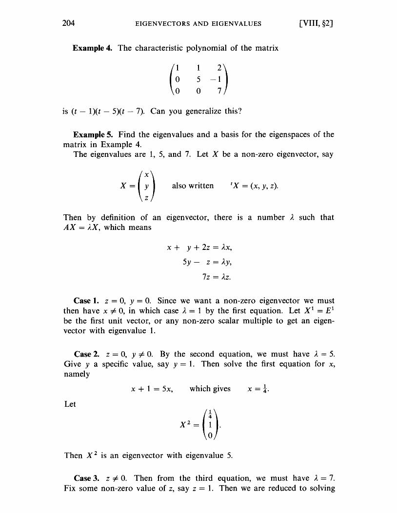
204 EIGENVECTORS AND EIGENVALUES [VIII, §2]
Example 4. The characteristic polynomial of the matrix
is (t - 1)( t - 5)( t - 7). Can you generalize this?
Example 5. Find the eigenvalues and a basis for the eigenspaces of the matrix in Example 4.
The eigenvalues are 1, 5, and 7. Let X be a non-zero eigenvector, say
also written tx = (x, y, z).
Then by definition of an eigenvector, there is a number A such that AX = AX, which means
x + y + 2z = AX,
5y - Z = AY,
7z = AZ.
Case 1. Z = 0, y = o. Since we want a non-zero eigenvector we must then have X =1= 0, in which case A = 1 by the first equation. Let Xl = E1 be the first unit vector, or any non-zero scalar multiple to get an eigenvector with eigenvalue 1.
Case 2. Z = 0, y =1= o. By the second equation, we must have A = 5. Give y a specific value, say y = 1. Then solve the first equation for x, namely
X + 1 = 5x, which gives X =!. Let
Then X 2 is an eigenvector with eigenvalue 5.
Case 3. Z =1= O. Then from the third equation, we must have A = 7. Fix some non-zero value of z, say Z = 1. Then we are reduced to solving
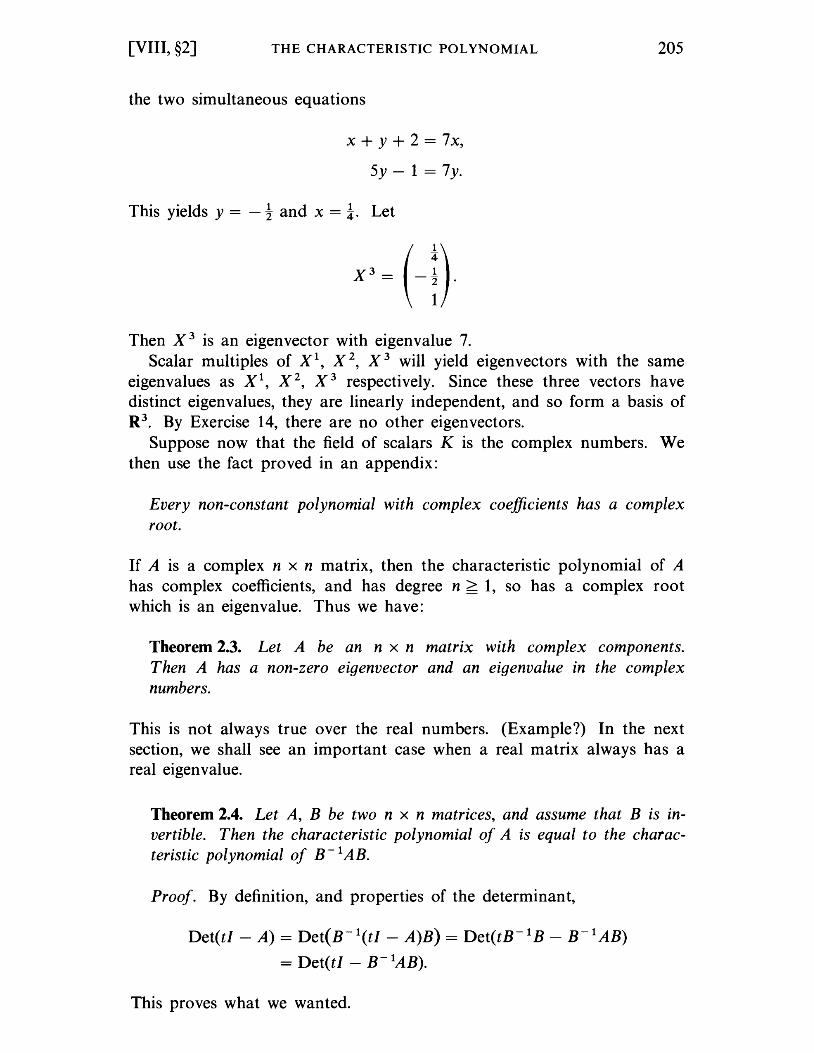
[VIII, §2] THE CHARACTERISTIC POLYNOMIAL
the two simultaneous equations
x + y + 2 = 7x,
5y - 1 = 7y.
This yields y = - -t and x = !. Let
Then X 3 is an eigenvector with eigenvalue 7.
205
Scalar multiples of Xl, X 2, X 3 will yield eigenvectors with the same eigenvalues as xl, X 2
, X 3 respectively. Since these three vectors have distinct eigenvalues, they are linearly independent, and so form a basis of R3. By Exercise 14, there are no other eigenvectors.
Suppose now that the field of scalars K is the complex numbers. We then use the fact proved in an appendix:
Every non-constant polynomial with complex coefficients has a complex root.
If A is a complex n x n matrix, then the characteristic polynomial of A has complex coefficients, and has degree n > 1, so has a complex root which is an eigenvalue. Thus we have:
Theorem 2.3. Let A be an n x n matrix with complex components. Then A has a non-zero eigenvector and an eigenvalue in the complex numbers.
This is not always true over the real numbers. (Example?) In the next section, we shall see an important case when a real matrix always has a real eigenvalue.
Theorem 2.4. Let A, B be two n x n matrices, and assume that B is invertible. Then the characteristic polynomial of A is equal to the characteristic polynomial of B- 1 AB.
Proof. By definition, and properties of the determinant,
Det(tI - A) = Det(B- 1(tI - A)B) = Det(tB- 1 B - B- 1 AB)
= Det(tI - B- 1AB).
This proves what we wanted.
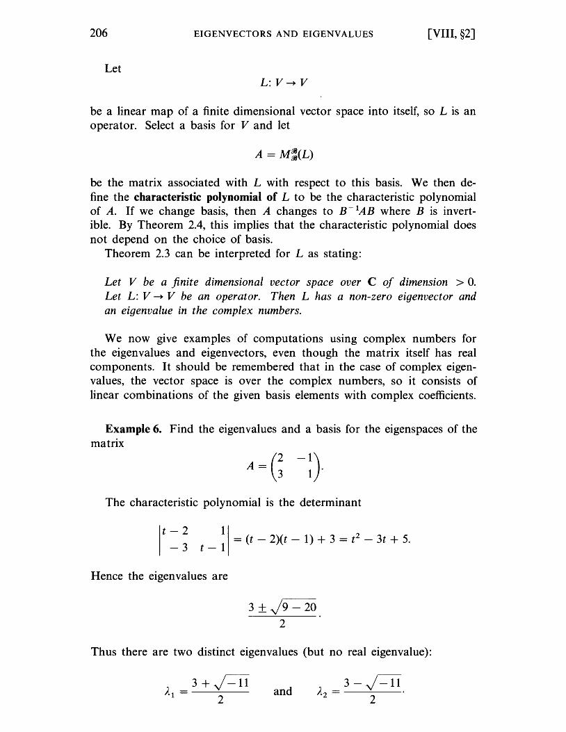
206 EIGENVECTORS AND EIGENVALUES [VIII, §2]
Let L:V~V
be a linear map of a finite dimensional vector space into itself, so L is an operator. Select a basis for V and let
be the matrix associated with L with respect to this basis. We then define the characteristic polynomial of L to be the characteristic polynomial of A. If we change basis, then A changes to B-1AB where B is invertible. By Theorem 2.4, this implies that the characteristic polynomial does not depend on the choice of basis.
Theorem 2.3 can be interpreted for L as stating:
Let V be a finite dimensional vector space over C of dimension > O. Let L: V ~ V be an operator. Then L has a non-zero eigenvector and an eigenvalue in the complex numbers.
We now give examples of computations using complex numbers for the eigenvalues and eigenvectors, even though the matrix itself has real components. It should be remembered that in the case of complex eigenvalues, the vector space is over the complex numbers, so it consists of linear combinations of the given basis elements with complex coefficients.
Example 6. Find the eigenvalues and a basis for the eigenspaces of the matrix
A=G -1) 1 .
The characteristic polynomial is the determinant
t - 2
-3 1
= (t - 2)(t - 1) + 3 = t2 - 3t + 5.
t - 1
Hence the eigenvalues are
3 ±)9 - 20 2
Thus there are two distinct eigenvalues (but no real eigenvalue):
and
[VIII, §2] THE CHARACTERISTIC POLYNOMIAL 207
Let X = (;) with not both x, y equal to O. Then X is an eigenvector if
and only if AX = AX, that is:
2x - Y = AX,
3x + y = AY,
where A is an eigenvalue. This system is equivalent with
(2 - A)X - Y = 0,
3x + (1 - A)Y = o.
We give X, say, an arbitrary value, for instance X = 1 and solve for y, so Y = (2 - A) from the first equation. Then we obtain the eigenvectors
and
Remark. We solved for Y from one of the equations. This is consistent with the other because A is an eigenvalue. Indeed, if you substitute x = 1 and Y = 2 - A on the left in the second equation, you get
3 + (1 - A)(2 - A) = 0
because A is a root of the characteristic polynomial.
Then X(A I ) is a basis for the one-dimensional eigenspace of AI' and X(A 2 ) is a basis for the one-dimensional eigenspace of A2 •
Example 7. Find the eigenvalues and a basis for the eigenspaces of the matrix
1
1
o
-1) o . 1
We compute the characteristic polynomial, which is the determinant
t-1 -1 1 o t - 1 0
-1 0 t-1
easily computed to be
P(t) = (t - 1)(t2 - 2t + 2).
208 EIGENVECTORS AND EIGENVALUES [VIII, §2]
Now we meet the problem of finding the roots of P(t) as real numbers or complex numbers. By the quadratic formula, the roots of t 2
- 2t + 2 are given by
The whole theory of linear algebra could have been done over the complex numbers, and the eigenvalues of the given matrix can also be defined over the complex numbers. Then from the computation of the roots above, we see that the only real eigenvalue is 1; and that there are two complex eigenvalues, namely
1 + v'-l and I-Fl· We let these eigenvalues be
Let
be a non-zero vector. Then X is an eigenvector for A if and only if the following equations are satisfied with some eigenvalue A:
x + y - Z = AX,
y = AY,
X + Z = AZ.
This system is equivalent with
(1 - A)X + Y - Z = 0,
(1 - A)Y = 0,
X + (1 - A)Z = o.
Case 1. A = 1. Then the second equation will hold for any value of y. Let us put y = 1. From the first equation we get Z = 1, and from the third equation we get X = O. Hence we get a first eigenvector
[VIII, §2] THE CHARACTERISTIC POLYNOMIAL 209
Case 2. A =1= 1. Then from the second equation we must have y = O. Now we can solve the system arising from the first and third equations:
(1 - A)X - Z = 0,
x + (1 - A)Z = O.
If these equations were independent, then the only solutions would be x = Z = O. This cannot be the case, since there must be a non-zero eigenvector with the given eigenvalue. Actually you can check directly that the second equation is equal to (A - 1) times the first. In any case, we give one of the variables an arbitrary value, and solve for the other. For instance, let Z = 1. Then x = 1/(1 - A). Thus we get the eigenvector
(
1/(1 - A)) X(A) = 0 .
1
We can substitute A = Ai and A = A2 to get the eigenvectors with the eigenvalues Ai and A2 respectively.
In this way we have found three eigenvectors with distinct eigenvalues, namely
Example 8. Find the eigenvalues and a basis for the eigenspaces of the matrix
(-~ -1
1
-1
The characteristic polynomial is
t - 1
2 - 1
1
t - 1
1
-2 - 3 = (t - 1)3 - (t - 1) - 1.
t - 1
The eigenvalues are the roots of this cubic equation. In general it is not easy to find such roots, and this is the case in the present instance. Let u = t - 1. In terms of u the polynomial can be written
Q(u) = u3 - U - 1.
210 EIGENVECTORS AND EIGENVALUES [VIII, §2]
From arithmetic, the only rational roots must be integers, and must divide 1, so the only possible rational roots are + 1, which are not roots. Hence there is no rational eigenvalue. But a cubic equation has the general shape as shown on the figure:
-1/)3 1/)3
Figure 1
This means that there is at least one real root. If you know calculus, then you have tools to be able to determine the relative maximum and relative minimum, you will find that the function u3
- u - 1 has its rela-
tive maximum at u == -1/)3, and that Q( -1/)3) is negative. Hence there is only one real root. The other "two roots are complex. This is as far as we are able to go with the means at hand. In any case, we give these roots a name, and let the eigenvalues be
They are all distinct. We can, however, find the eigenvectors In terms of the eigenvalues.
Let
be a non-zero vector. Then X is an eigenvector if and only if AX == AX, that is:
x -- y + 2z == AX,
-2x + y + 3z == Ay,
X - Y + Z == Az.
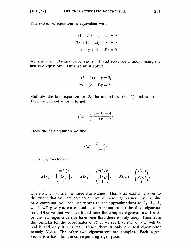
[VIII, §2] THE CHARACTERISTIC POLYNOMIAL
This system of equations is equivalent with
(1 - A)X - Y + 2z = 0,
- 2x + (1 - A)Y + 3z = 0,
x - Y + (1 - A)Z = O.
211
We give Z an arbitrary value, say Z = 1 and solve for x and y using the first two equations. Thus we must solve:
(A - l)x + y = 2,
2x+(A-l)y=3.
Multiply the first equation by 2, the second by (A - 1) and subtract. Then we can solve for y to get
3(A-l)-4 y( A.) = (A. _ 1)2 - 2 .
From the first equation we find
Hence eigenvectors are
2-y X(A) = --.
A-I
where AI' A2 , A3 are the three eigenvalues. This is an explicit answer to the extent that you are able to determine these eigenvalues. By machine or a computer, you can use means to get approximations to AI' A2 , A3 which will give you corresponding approximations to the three eigenvectors. Observe that we have found here the complex eigenvectors. Let Al be the real eigenvalue (we have seen that there is only one). Then from the formulas for the coordinates of X(A), we see that yeA) or X(A) will be real if and only if A is real. Hence there is only one real eigenvector namely X(A 1). The other two eigenvectors are complex. Each eigenvector is a basis for the corresponding eigenspace.
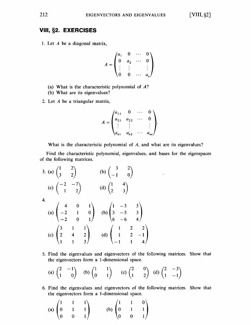
212 EIGENVECTORS AND EIGENVALUES
VIII, §2. EXERCISES
1. Let A be a diagonal matrix,
o
J). A=
o
(a) What is the characteristic polynomial of A? (b) What are its eigenvalues?
2. Let A be a triangular matrix,
A=
[VIII, §2]
What is the characteristic polynomial of A, and what are its eigenvalues?
Find the characteristic polynomial, eigenvalues, and bases for the eigenspaces of the following matrices.
3. (a) G ~) (b) ( _ ~ ~) (-2 -7) (c) 1 2 (d) G ~)
4.
(a) ( -~ 0
D (b) (:
-3
!) 1 -5 -2 0 -6
(c) G 1
n (-: 2
-D 4 (d) 2
1 1
5. Find the eigenvalues and eigenvectors of the following matrices. Show that the eigenvectors form a I-dimensional space.
(a) G -~) (b) G ~) (c) G ~) (d) G -3) -1
6. Find the eigenvalues and eigenvectors of the following matrices. Show that the eigenvectors form a I-dimensional space.
(a) G 1
:) (b) G 1
D 1 1
0 0
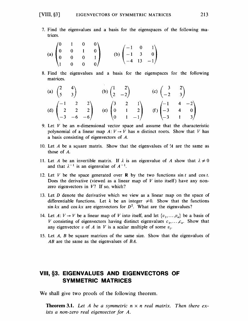
[VIII, §3] EIGENVECTORS OF SYMMETRIC MATRICES 213
7. Find the eigenvalues and a basis for the eigenspaces of the following matrices.
(a) (~ 1 0
!) ( -1
0 0 1
(b) -1 3 0 0
-4 13 0 0
8. Find the eigen val ues and a basis for the matrices.
(a) (
25 (b) G -~)
(- ~ ~ ~) (e) (~ ~ ~) -3 -6 -6 0 1-1
(d)
-D eigenspaces
(c) (_~
(
-1
(f) -3
-3
for the following
9. Let V be an n-dimensional vector space and assume that the characteristic polynomial of a linear map A: V -+ V has n distinct roots. Show that V has a basis consisting of eigenvectors of A.
10. Let A be a square matrix. Show that the eigenvalues of ~ are the same as those of A.
11. Let A be an invertible matrix. If'{ is an eigenvalue of A show that ,{ =1= 0 and that ,{ -1 is an eigenvalue of A-I.
12. Let V be the space generated over R by the two functions sin t and cos t. Does the derivative (viewed as a linear map of V into itself) have any nonzero eigenvectors in V? If so, which?
13. Let D denote the derivative which we view as a linear map on the space of differentiable functions. Let k be an integer =1= o. Show that the functions sin kx and cos kx are eigenvectors for D2. What are the eigenvalues?
14. Let A: V -+ V be a linear map of V into itself, and let {VI' ... ,Vn } be a basis of V consisting of eigenvectors having distinct eigenvalues C 1' ... 'Cn. Show that any eigenvector V of A in V is a scalar mUltiple of some Vi.
15. Let A, B be square matrices of the same size. Show that the eigenvalues of AB are the same as the eigenvalues of BA.
VIII, §3. EIGENVALUES AND EIGENVECTORS OF SYMMETRIC MATRICES
We shall give two proofs of the following theorem.
Theorem 3.1. Let A be a symmetric n x n real matrix. Then there exists a non-zero real eigenvector for A.
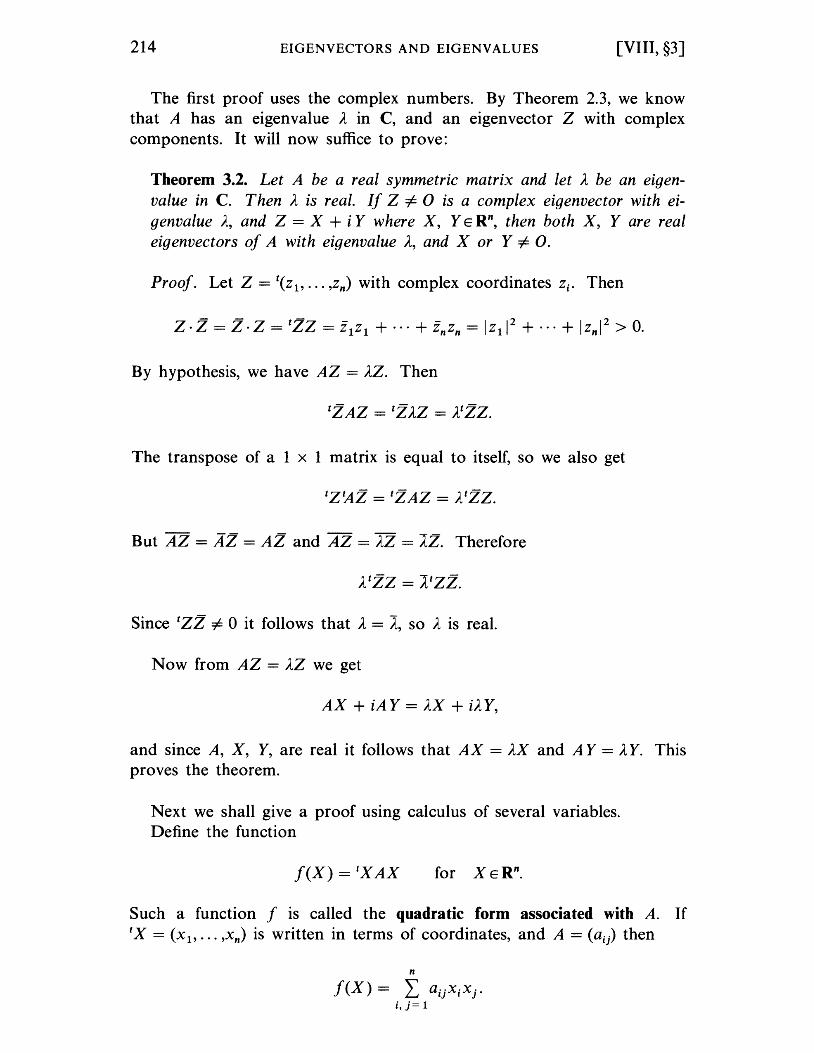
214 EIGENVECTORS AND EIGENVALUES [VIII, §3]
The first proof uses the complex numbers. By Theorem 2.3, we know that A has an eigenvalue A in C, and an eigenvector Z with complex components. It will now suffice to prove:
Theorem 3.2. Let A be a real symmetric matrix and let A be an eigenvalue in C. Then A is real. If Z =1= 0 is a complex eigenvector with eigenvalue A, and Z = X + i Y where X, Y ERn, then both X, Yare real eigenvectors of A with eigenvalue A, and X or Y i= O.
Proof. Let Z = t(Zl' ... ,zn) with complex coordinates Zi. Then
By hypothesis, we have AZ = AZ. Then
The transpose of a 1 x 1 matrix is equal to itself, so we also get
But AZ = AZ = AZ and AZ = AZ = A:Z. Therefore
Since tzZ i= 0 it follows that A = ~, so A is real.
Now from AZ = AZ we get
AX + iA Y = AX + iA Y,
and since A, X, Y, are real it follows that AX = AX and A Y = AY. This proves the theorem.
Next we shall give a proof using calculus of several variables. Define the function
f(X) = tXAX
Such a function f is called the quadratic form associated with A. If tx = (Xl' ... ,Xn) is written in terms of coordinates, and A = (aij) then
n
f(X) = L aijxixj •
i, j= 1
[VIII, §3] EIGENVECTORS OF SYMMETRIC MATRICES 215
Example. Let
Let tx = (x, y). Then
More generally, let
Then
Example. Suppose we are given a quadratic expression
f(x, y) = 3x2 + 5xy - 4y2.
Then it is the quadratic form associated with the symmetric matrix
A = 2 (
3 ~) ~ -4
In many applications, one wants to find a maximum for such a function f on the unit sphere. Recall that the unit sphere is the set of all
points X such that IIXII = 1, where IIXII =JX.X. It is shown in analysis courses that a continuous function f as above necessarily has a maximum on the sphere. A maximum on the unit sphere is a point P such that IIPII = 1 and
f(P) > f(X) for all X with II X II = 1.
The next theorem relates this problem with the problem of finding eigenvectors.
Theorem 3.3. Let A be a real symmetric matrix, and let f(X) = tXAX be the associated quadratic form. Let P be a point on the unit sphere such that f(P) is a maximum for f on the sphere. Then P is an eigenvector for A. I n other words, there exists a number )., such that AP = )"P.
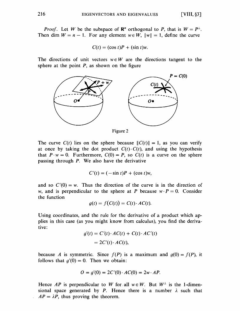
216 EIGENVECTORS AND EIGENVALUES [VIII, §3]
Proof. Let W be the subspace of Rn orthogonal to P, that is W = p.l. Then dim W = n - 1. For any element WE W, IIwll = 1, define the curve
C(t) = (cos t)P + (sin t)w.
The directions of unit vectors WE Ware the directions tangent to the sphere at the point P, as shown on the figure
p = C(O)
c~ ~..--------- .. -......
0-
Figure 2
The curve C(t) lies on the sphere because II C(t)11 = 1, as you can verify at once by taking the dot product C(t)· C(t), and using the hypothesis that p. W = O. Furthermore, C(O) = P, so C(t) is a curve on the sphere passing through P. We also have the derivative
C'(t) = ( - sin t)P + (cos t)w,
and so C'(O) = w. Thus the direction of the curve is in the direction of w, and is perpendicular to the sphere at P because W· P = O. Consider the function
get) = f( C(t)) = C(t)· AC(t).
Using coordinates, and the rule for the derivative of a product which applies in this case (as you might know from calculus), you find the derivative:
g'(t) = C'(t)· AC(t) + C(t)· AC'(t)
= 2C'(t)· AC(t),
because A is symmetric. Since f(P) is a maximum and g(O) = f(P), it follows that g'(O) = O. Then we obtain:
o = g'(O) = 2C'(O)· AC(O) = 2w· AP.
Hence AP is perpendicular to W for. all WE W. But W.l is the 1-dimensional space generated by P. Hence there is a number )., such that AP = )"P, thus proving the theorem.
[VIII, §3] EIGENVECTORS OF SYMMETRIC MATRICES 217
Corollary 3.4. The maximum value of f on the unit sphere is equal to the largest eigenvalue of A.
Proof. Let A be any eigenvalue and let P be an eigenvector on the unit sphere, so IIPII = 1. Then
Thus the value of f at an eigenvector on the unit sphere is equal to the eigenvalue. Theorem 3.3 tells us that the maximum of f on the unit sphere occurs at an eigenvector. Hence the maximum of f on the unit sphere is equal to the largest eigenvalue, as asserted.
Example. Let f(x, y) = 2X2 - 3xy + y2. Let A be the symmetric matrix associated with f. Find the eigenvectors of A on the unit circle, and find the maximum of f on the unit circle.
First we note that f is the quadratic form associated with the matrix
=( 2 -i) A 3 . -2 1
By Theorem 3.3 a maximum must occur at an eigenvector, so we first find the eigenvalues and eigenvectors.
The characteristic polynomial is the determinant
t - 2
Then the eigenvalues are
3 "2
3
2 = t2 - 3t _ i. t - 1
For the eigenvectors, we must solve
2x - iy = AX,
-ix + y = Ay.
Putting X = 1 this gives the possible eigenvectors
218 EIGENVECTORS AND EIGENVALUES [VIII, §4]
Thus there are two such eigenvectors, up to non-zero scalar multiples. The eigenvectors lying on the unit circle are therefore
P A _ X(A) ( ) - IIX(A)II with and
By Corollary 3.4 the maximum is the point with the bigger eigenvalue, and must therefore be the point
peA) with
The maximum value of f on the unit circle is (3 + jiO)/2. By the same token, the minimum value of f on the unit circle IS
(3 - jiO)/2.
VIII, §3. EXERCISES
1. Find the eigenvalues of the following matrices, and the maximum value of the associated quadratic forms on the unit circle.
( 2 -1) (a) -1 2 (b) G ~)
2. Same question, except find the maximum on the unit sphere.
(a) (-~ -~ -~) (b) (-~ -~ -~) o -1 1 0 -1 2
3. Find the maximum and minimum of the function
f(x, y) = 3x2 + 5xy - 4y2
on the unit circle.
VIII, §4. DIAGONALIZATION OF A SYMMETRIC LINEAR MAP
Throughout this section, unless otherwise specified, we let V be a vector space of dimension n over R, with a positive definite scalar product.
We shall give an application of the existence of eigenvectors proved in §3. We let
A:V~V
[VIII, §4] DIAGONALIZATION OF A SYMMETRIC LINEAR MAP 219
be a linear map. Recall that A IS symmetric (with respect to the scalar product) if we have the relation
<Av, W) = <v, Aw) 'for all v, WE V.
We can reformulate Theorem 3.1 as follows:
Theorem 4.1. Let V be a finite dimensional vector space with a positive definite scalar product. Let A: V ~ V be a symmetric linear map. Then A has a nonzero eigenvector.
Let W be a subspace of V, and let A: V ~ V be a symmetric linear map. We say that W is stable under A if A(W) c W, that is for all u E W we have Au E W. Sometimes one also says that W is invariant under A.
Theorem 4.2. Let A: V ~ V be a symmetric linear map. Let v be a non-zero eigenvector of A. If w is an element of V, perpendicular to v, then A w is also perpendicular to v.
If W is a subspace of V which is stable under A, then W.l is also stable under A.
Proof. Suppose first that v is an eigenvector of A. Then
<Aw, v) = <w, Av) = <w, AV) = A<w, v) = o.
Hence A w is also perpendicular to v. Second, suppose W is stable under A. Let u E W.l. Then for all WE W
we have:
<Au, w) = <u, Aw) = 0
by the assumption that Aw E W. Hence Au E W.l, thus proving the second assertion.
Theorem 4.3 (Spectral theorem). Let V be a finite dimensional vector space over the real numbers, of dimension n > 0, and with a positive definite scalar product. Let
A:V~V
be a linear map, symmetric with respect to the scalar product. Then V has an orthonormal basis consisting of eigenvectors.
Proof. By Theorem 3.1, there exists a non-zero eigenvector v for A. Let W be the one-dimensional space generated by v. Then W is stable under A. By Theorem 4.2, W.l is also stable under A and is a vector
220 EIGENVECTORS AND EIGENVALUES [VIII, §4]
space of dimension n - 1. We may then view A as gIvIng a symmetric linear map of W-L into itself. We can then repeat the procedure. We put v = V1 , and by induction we can find a basis {v 2 , ••• ,vn} of W-L consisting of eigenvectors. Then
is an orthogonal basis of V consisting of eigenvectors. We divide each vector by its norm to get an orthonormal basis, as desired.
If {e 1 , ••• ,en} is an orthonormal basis of V such that each ei is an eigen vector, then the matrix of A with respect to this basis is diagonal, and the diagonal elements are precisely the eigenvalues:
In such a simple representation, the effect of A then becomes much clearer than when A is represented by a more complicated matrix with respect to another basis.
A basis {v 1, ••• ,vn } such that each Vi is an eigenvector for A is called a spectral basis for A. We also say that this basis diagonalizes A, because the matrix of A with respect to this basis is a diagonal basis.
Example. We give an application to linear differential equations. Let A be an n x n symmetric real matrix. We want to find the solutions in Rn of the differential equation
where
dX(t) --=AX(t)
dt '
is given in terms of coordinates which are functions of t, and
Writing this equation in terms of arbitrary coordinates is messy. So let us forget at first about coordinates, and view Rn as an n-dimensional
[VIII, §4] DIAGONALIZATION OF A SYMMETRIC LINEAR MAP 221
vector space with a posItIve definite scalar product. We choose an orthonormal basis of V (usually different from the original basis) consisting of eigenvectors of A. Now with respect to this new basis, we can identify V with Rn with new coordinates which we denote by Y1' ... ,Yn. With respect to these new coordinates, the matrix of the linear map LA is
where A1, ••• ,An are the eigenvalues. But in terms of these more convenient coordinates, our differential equation simply reads
Thus the most general solution is of the form
with some constant ci •
The moral of this example is that one should not select a basis too quickly, and one should use as often as possible a notation without coordinates, until a choice of coordinates becomes imperative to make the solution of a problem simpler.
Theorem 4.4. Let A be a symmetric real n x n matrix. Then there exists an n x n real unitary matrix U such that
is a diaponal matrix.
Proof. We view A as the associated matrix of a symmetric linear map
relative to the standard basis [lA = {el, ... ,en}. By Theorem 4.3 we can find an orthonormal basis [lA' = {w 1, ••• ,wn } of Rn such that
222 EIGENVECTORS AND EIGENVALUES [VIII, §4J
is diagonal. Let U = M::,(id). Then U -1 AU IS diagonal. Furthermore U is unitary. Indeed, let U = (c ij ). Then
n
Wi = L Cjiej j= 1
for i = 1, ... ,no
The conditions <Wi' Wi) = 1 and <Wi' Wj ) = 0 if i i= j are immediately seen to mean that
tuu = I that is
This proves Theorem 4.4.
Remark. Theorem 4.4 shows us how to obtain all symmetric real matrices. Every symmetric real matrix A can be written in the form
tUBU,
where B is a diagonal matrix and U is real unitary.
VIII, §4. EXERCISES
1. Suppose that A is a diagonal n x n matrix. For any X ERn, what is tx AX in terms of the coordinates of X and the diagonal elements of A?
2. Let
be a diagonal matrix with A 1 ~ 0, ... ,An ~ o. Show that there exists an n x n diagonal matrix B such that B2 = A.
3. Let V be a finite dimensional vector space with a posItIve definite scalar product. Let A: V --+ V be a symmetric linear map. We say that A is positive definite if (Av, v) > 0 for all VE V and v i= o. Prove: (a) if A is positive definite, then all eigenvalues are > o. (b) If A is positive definite, then there exists a symmetric linear map B such
that B2 = A and BA = AB. What are the eigenvalues of B? [Hint: Use a basis of V consisting of eigenvectors.]
4. We say that A is semipositive if (Av, v) ~ 0 for all VE V. Prove the analogues of (a), (b) of Exercise 3 when A is only assumed semipositive. Thus the eigenvalues are ~ 0, and there exists a symmetric linear map B such that B2 = A.
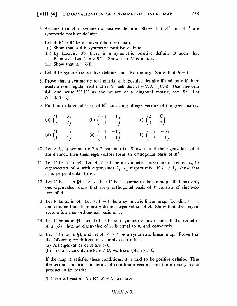
[VIII, §4] DIAGONALIZATION OF A SYMMETRIC LINEAR MAP 223
5. Assume that A is symmetric positive definite. Show that A 2 and A-I are symmetric positive definite.
6. Let A: Rn --+ Rn be an invertible linear map. (i) Show that ~A is symmetric positive definite.
(ii) By Exercise 3b, there is a symmetric positIve definite B such that B2 = ~A. Let U = AB - 1. Show that U is unitary.
(iii) Show that A = U B.
7. Let B be symmetric positive definite and also unitary. Show that B = I.
8. Prove that a symmetric real matrix A is positive definite if and only if there exists a non-singular real matrix N such that A = tNN. [Hint: Use Theorem 4.4, and write tu AU as the square of a diagonal matrix, say B2. Let N=UB- 1
.]
9. Find an orthogonal basis of R2 consisting of eigenvectors of the given matrix.
(a) G ~) (b) (-~ ~) (c) (~ ~) (d) G ~) (e) (-~ -~) (f) (-~ -:)
10. Let A be a symmetric 2 x 2 real matrix. Show that if the eigenvalues of A are distinct, then their eigenvectors form an orthogonal basis of R 2 •
11. Let V be as in §4. Let A: V --+ V be a symmetric linear map. Let VI' V 2 be eigenvectors of A with eigenyalues AI, A2 respectively. If Al i= A2, show that VI is perpendicular to v2 •
12. Let V be as in §4. Let A: V --+ V be a symmetric linear map. If A has only one eigenvalue, show that every orthogonal basis of V consists of eigenvectors of A.
13. Let V be as in §4. Let A: V --+ V be a symmetric linear map. Let dim V = n, and assume that there are n distinct eigenvalues of A. Show that their eigenvectors form an orthogonal basis of v.
14. Let V be as in §4. Let A: V --+ V be a symmetric linear map. If the kernel of A is {O}, then no eigenvalue of A is equal to 0, and conversely.
15. Let V be as in §4, and let A: V --+ V be a symmetric linear map. Prove that the following conditions on A imply each other. (a) All eigenvalues of A are > o. (b) For all elements VE V, V i= 0, we have (Av, v) > O.
If the map A satisfies these conditions, it is said to be positive definite. Thus the second condition, in terms of coordinate vectors and the ordinary scalar product in Rn reads:
(b/) For all vectors X ERn, X i= 0, we have
tXAX > O.
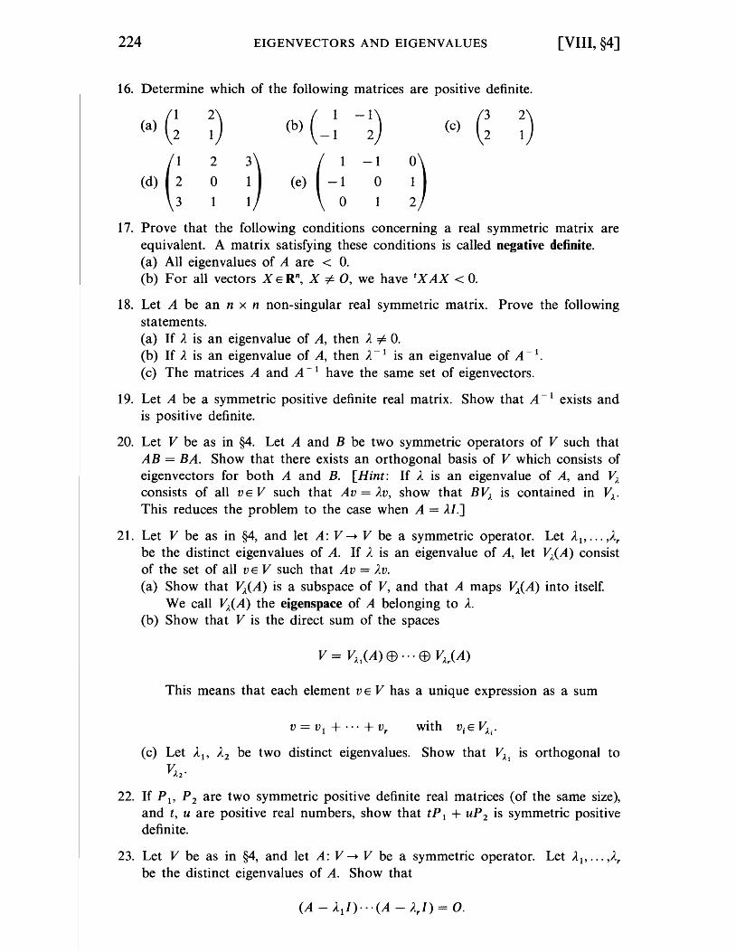
224 EIGENVECTORS AND EIGENVALUES
16. Determine which of the following matrices are positive definite.
(a) G
(d) G ~) 2
o 1
-1
o 1
(c) ~)
D
[VIII, §4]
17. Prove that the following conditions concerning a real symmetric matrix are equivalent. A matrix satisfying these conditions is called negative definite. (a) All eigenvalues of A are < o. (b) For all vectors XERn, X =I 0, we have tXAX < O.
18. Let A be an n x n non-singular real symmetric matrix. Prove the following statements. (a) If A is an eigenvalue of A, then A =I o. (b) If A is an eigenvalue of A, then A -1 is an eigenvalue of A -1.
(c) The matrices A and A -1 have the same set of eigenvectors.
19. Let A be a symmetric positive definite real matrix. Show that A - 1 exists and is positive definite.
20. Let V be as in §4. Let A and B be two symmetric operators of V such that AB = BA. Show that there exists an orthogonal basis of V which consists of eigenvectors for both A and B. [Hint: If A is an eigenvalue of A, and V;. consists of all v E V such that Av = AV, show that BV;. is contained in V;.. This reduces the problem to the case when A = AI.]
21. Let V be as in §4, and let A: V --+ V be a symmetric operator. Let A l' ... ,Ar be the distinct eigenvalues of A. If A is an eigenvalue of A, let V;.(A) consist of the set of all VE V such that Av = AV. (a) Show that V;.(A) is a subspace of V, and that A maps V;.(A) into itself.
We call V;.(A) the eigenspace of A belonging to A. (b) Show that V is the direct sum of the spaces
This means that each element v E V has a unique expression as a sum
v = v1 + ... + Vr
(c) Let A1, A2 be two distinct eigenvalues. Show that V;'l is orthogonal to V;. 2 •
22. If P l' P 2 are two symmetric positive definite real matrices (of the same size), and t, u are positive real numbers, show that tP 1 + uP 2 is symmetric positive definite.
23. Let V be as in §4, and let A: V --+ V be a symmetric operator. Let A l' ... ,Ar be the distinct eigenvalues of A. Show that
(A - A 1 I) ... (A - Ar I) = O.
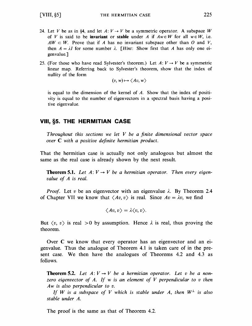
[VIII, §5] THE HERMITIAN CASE 225
24. Let V be as in §4, and let A: V ~ V be a symmetric operator. A subspace W of V is said to be invariant or stable under A if Aw E W for all WE W, i.e. AWe W. Prove that if A has no invariant subspace other than 0 and V, then A = AI for some number A. [Hint: Show first that A has only one eigenvalue.]
25. (For those who have read Sylvester's theorem.) Let A: V ~ V be a symmetric linear map. Referring back to Sylvester's theorem, show that the index of nullity of the form
(v, w) ~ (Av, w)
is equal to the dimension of the kernel of A. Show that the index of positivity is equal to the number of eigenvectors in a spectral basis having a positive eigenvalue.
VIII, §5. THE HERMITIAN CASE
Throughout this sections we let V be a finite dimensional vector space over C with a positive definite hermitian product.
That the hermitian case is actually not only analogous but almost the same as the real case is already shown by the next result.
Theorem 5.1. Let A: V -+ V be a hermitian operator. Then every eigenvalue of A is real.
Proof. Let v be an eigenvector with an eigenvalue A. By Theorem 2.4 of Chapter VII we know that <Av, v) is real. Since Av = AV, we find
<Av, v) = A<V, v>.
But <v, v) is real >0 by assumption. Hence A is real, thus proving the theorem.
Over C we know that every operator has an eigenvector and an eigenvalue. Thus the analogue of Theorem 4.1 is taken care of in the present case. We then have the analogues of Theorems 4.2 and 4.3 as follows.
Theorem 5.2. Let A: V -+ V be a hermitian operator. Let v be a nonzero eigenvector of A. If w is an element of V perpendicular to v then A w is also perpendicular to v.
If W is a subspace of V which is stable under A, then W-L is also stable under A.
The proof is the same as that of Theorem 4.2.
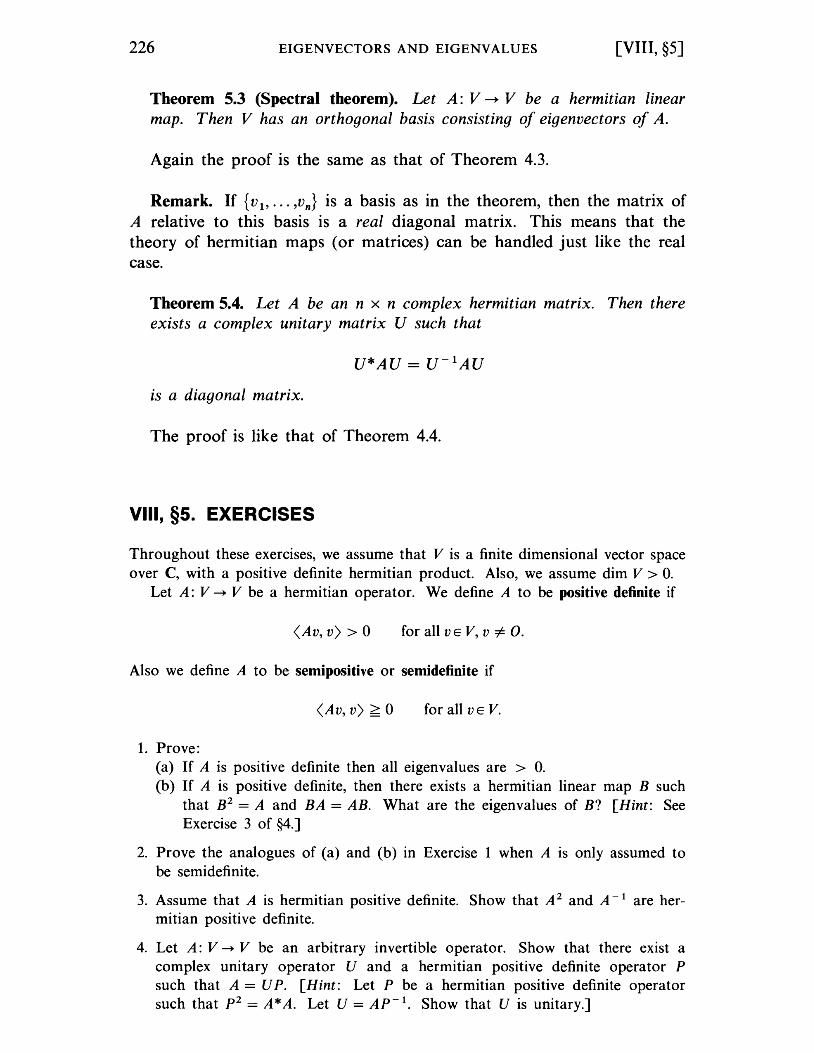
226 EIGENVECTORS AND EIGENVALUES [VIII, §5]
Theorem 5.3 (Spectral theorem). Let A: V ~ V be a hermitian linear map. Then V has an orthogonal basis consisting of eigenvectors of A.
Again the proof is the same as that of Theorem 4.3.
Remark. If {v l , ... ,vn} is a basis as in the theorem, then the matrix of A relative to this basis is a real diagonal matrix. This means that the theory of hermitian maps (or matrices) can be handled just like the real case.
Theorem 5.4. Let A be an n x n complex hermitian matrix. Then there exists a complex unitary matrix U such that
U*AU = U-lAU
is a diagonal matrix.
The proof is like that of Theorem 4.4.
VIII, §5. EXERCISES
Throughout these exercises, we assume that V is a finite dimensional vector space over C, with a positive definite hermitian product. Also, we assume dim V > o.
Let A: V --+ V be a hermitian operator. We define A to be positive definite if
<Av, v) > 0 for all v E V, v # O.
Also we define A to be semi positive or semidefinite if
<Av, v) ~ 0 forallvEV.
1. Prove: (a) If A is positive definite then all eigenvalues are > o. (b) If A is positive definite, then there exists a hermitian linear map B such
that B2 = A and BA = AB. What are the eigenvalues of B? [Hint: See Exercise 3 of §4.]
2. Prove the analogues of (a) and (b) in Exercise 1 when A is only assumed to be semidefinite.
3. Assume that A is hermitian positive definite. Show that A 2 and A-I are hermitian positive definite.
4. Let A: V --+ V be an arbitrary invertible operator. Show that there exist a complex unitary operator U and a hermitian positive definite operator P such that A = UP. [Hint: Let P be a hermitian positive definite operator such that p 2 = A * A. Let U = AP - 1. Show that U is unitary.]
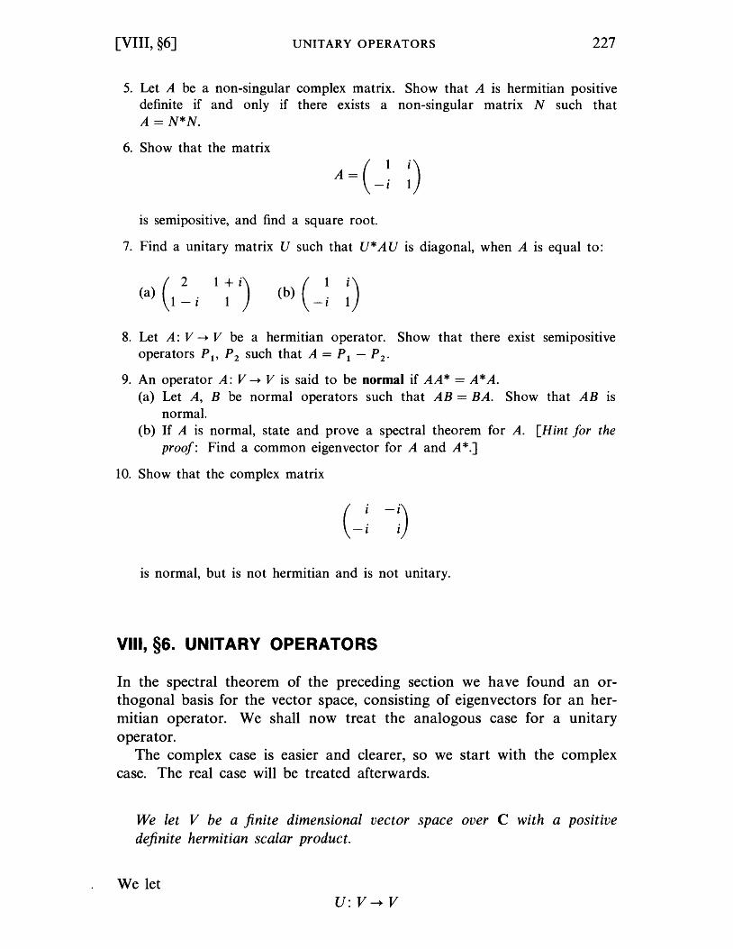
[VIII, §6] UNITARY OPERATORS 227
5. Let A be a non-singular complex matrix. Show that A is hermitian positive definite if and only if there exists a non-singular matrix N such that A = N*N.
6. Show that the matrix
( Ii) A= -i 1
is semipositive, and find a square root.
7. Find a unitary matrix U such that U* A U is diagonal, when A is equal to:
( 2 1 +1 i)
(a) 1 - i (b) (_~ :)
8. Let A: V ~ V be a hermitian operator. Show that there exist semipositive operators PI' P 2 such that A = PI - P 2 •
9. An operator A: V ~ V is said to be normal if AA * = A * A. (a) Let A, B be normal operators such that AB = BA. Show that AB is
normal. (b) If A is normal, state and prove a spectral theorem for A. [Hint for the
proof: Find a common eigenvector for A and A*.]
10. Show that the complex matrix
( ~ -~) -l l
is normal, but is not hermitian and is not unitary.
VIII, §6. UNITARY OPERATORS
In the spectral theorem of the preceding section we have found an orthogonal basis for the vector space, consisting of eigenvectors for an hermitian operator. We shall now treat the analogous case for a unitary operator.
The complex case is easier and clearer, so we start with the complex case. The real case will be treated afterwards.
We let V be a finite dimensional vector space over C with a positive definite hermitian scalar product.
We let U:V~V
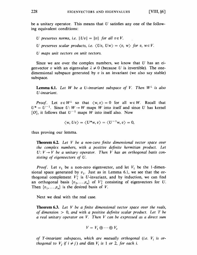
228 EIGENVECTORS AND EIGENVALUES [VIII, §6]
be a unitary operator. This means that U satisfies anyone of the following equivalent conditions:
U preserves norms, i.e. II Uvll = Ilvll for all VE v. U preserves scalar products, i.e. <Uv, Uw> = <v, w> for v, WE V.
U maps unit vectors on unit vectors.
Since we are over the complex numbers, we know that U has an eigenvector v with an eigenvalue A i= 0 (because U is invertible). The onedimensional subspace generated by v is an invariant (we also say stable) subspace.
Lemma 6.1. Let W be a U-invariant subspace of V. Then W-L is also U -invariant.
Proof. Let VEW-L so that <w,v>=O for all WEW. Recall that u* = U - 1. Since U: W ~ W maps W into itself and since U has kernel {O}, it follows that U- 1 maps W into itself also. Now
<W, Uv) = <U*w, v) = <U- 1w, v) = 0,
thus proving our lemma.
Theorem 6.2. Let V be a non-zero finite dimensional vector space over the complex numbers, with a positive definite hermitian product. Let U: V ~ V be a unitary operator. Then V has an orthogonal basis consisting of eigenvectors of U.
Proof. Let v1 be a non-zero eigenvector, and let V1 be the I-dimensional space generated by v1• Just as in Lemma 6.1, we see that the orthogonal complement vt is U-invariant, and by induction, we can find an orthogonal basis {v 2 , ••• ,vn} of vt consisting of eigenvectors for U. Then {v 1, ... ,vn } is the desired basis of v.
Next we deal with the real case.
Theorem 6.3. Let V be a finite dimensional vector space over the reals, of dimension > 0, and with a positive definite scalar product. Let T be a real unitary operator on V. Then V can be expressed as a direct sum
of T-invariant subspaces, which are mutually orthogonal (i.e. Vi is orthogonal to Vj if i i= j) and dim Vi is 1 or 2, for each i.
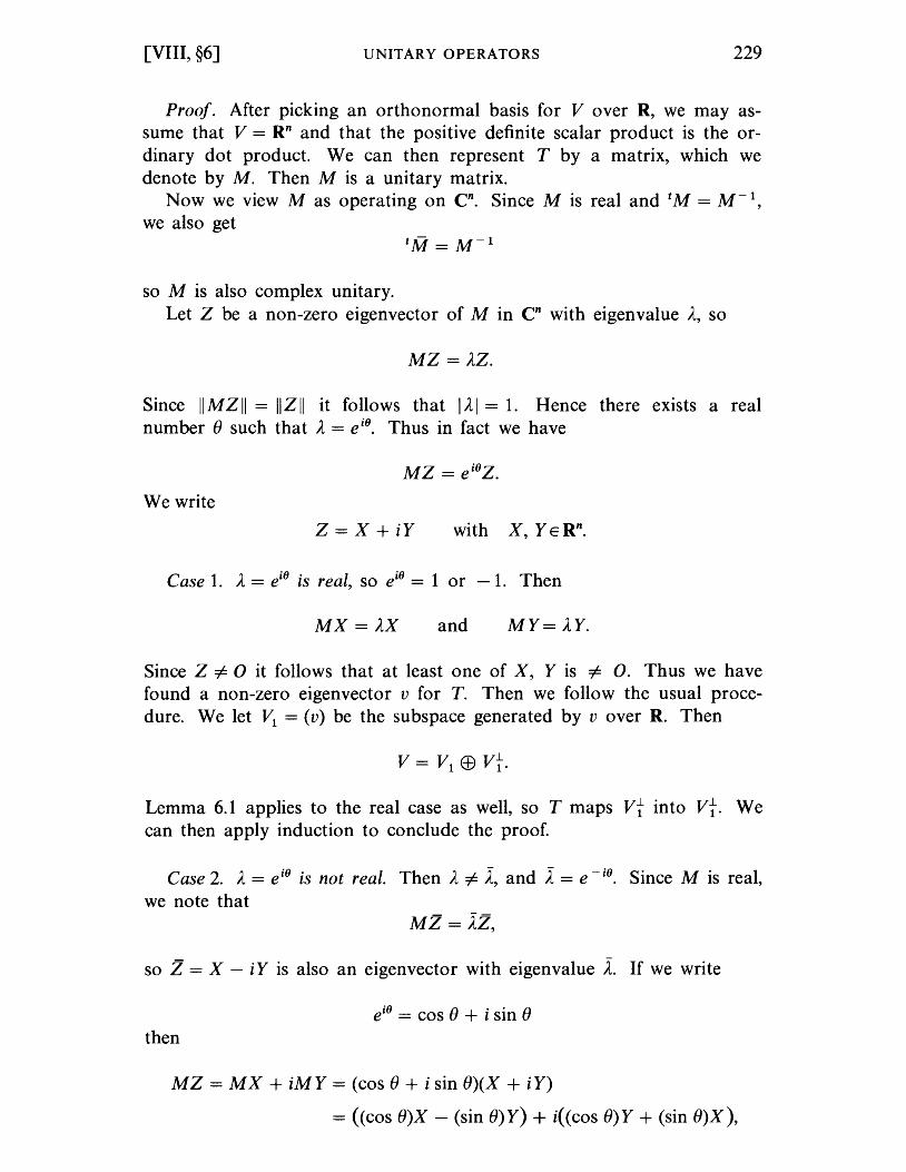
[VIII, §6] UNITARY OPERATORS 229
Proof. After picking an orthonormal basis for V over R, we may assume that V = Rn and that the positive definite scalar product is the ordinary dot product. We can then represent T by a matrix, which we denote by M. Then M is a unitary matrix.
Now we view M as operating on en. Since M is real and tM = M-l, we also get
so M is also complex unitary. Let Z be a non-zero eigenvector of M in en with eigenvalue A, so
MZ = AZ.
Since II M Z II = II Z II it follows that I A I = 1. Hence there exists a real number () such that A = ei8
• Thus in fact we have
We write
Z = X + iY
Case 1. A = ei8 is real, so ei8 = 1 or - 1. Then
MX=AX and MY= AY.
Since Z i= 0 it follows that at least one of X, Y is i= o. Thus we have found a non-zero eigenvector v for T. Then we follow the usual procedure. We let V1 = (v) be the subspace generated by v over R. Then
Lemma 6.1 applies to the real case as well, so T maps vi into vi. We can then apply induction to conclude the proof.
Case 2. A = e i8 is not real. Then A i= i, and i = e -w. Since M is real, we note that
so Z = X - iY is also an eigenvector with eigenvalue A. If we write
ei8 = cos () + i sin () then
MZ = MX + iMY = (cos () + i sin ())(X + iY)
= «cos ())X - (sin ()) Y) + i«cos ()) Y + (sin ())X),
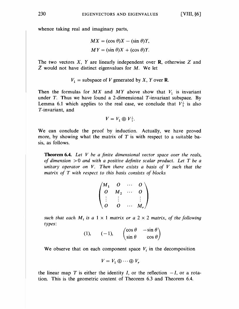
230 EIGENVECTORS AND EIGENVALUES
whence taking real and imaginary parts,
MX = (cos fJ)X - (sin fJ)Y,
MY = (sin fJ)X + (cos fJ)Y.
[VJII, §6]
The two vectors X, Yare linearly independent over R, otherwise Z and Z would not have distinct eigenvalues for M. We let
Vl = subspace of V generated by X, Y over R.
Then the formulas for MX and MY above show that VI IS Invariant under T. Thus we have found a 2-dimensional T-invariant subspace. By Lemma 6.1 which applies to the real case, we conclude that Vi is also T-invariant, and
We can conclude the proof by induction. Actually, we have proved more, by showing what the matrix of T is with respect to a suitable basis, as follows.
Theorem 6.4. Let V be a finite dimensional vector space over the reals, of dimension > 0 and with a positive definite scalar product. Let T be a unitary operator on V. Then there exists a basis of V such that the matrix of T with respect to this basis consists of blocks
o 0 M,
such that each Mi is a 1 x 1 matrix or a 2 x 2 matrix, of the following types:
(1), ( -1), (
COS fJ
sin fJ -sin fJ)
cos fJ
We observe that on each component space Vi in the decomposition
V= VIEB···EBV,
the linear map T is either the identity I, or the reflection - I, or a rotation. This is the geometric content of Theorem 6.3 and Theorem 6.4.
CHAPTER IX
Polynomials and Matrices
IX, §1. POLYNOMIALS
Let K be a field. By a polynomial over K we shall mean a formal expreSSIon
where t is a "variable". We have to explain how to form the sum and product of such expressions. Let
be another polynomial with hj E K. If, say, n > m we can write hj = 0 if j> m,
and then we can write the sum f + g as
Thus f + g is again a polynomial. If C E K, then
and hence cf is a polynomial. Thus polynomials form a vector space over K.
232 POLYNOMIALS AND MATRICES
We can also take the product of the two polynomials, fg, and
so that fg is again a polynomial. In fact, if we write
then
k
Ck = L aibk- i = aObk + a1bk- 1 + ... + akbo· i=O
[IX, §1]
All the preceding rules are probably familiar to you but we have recalled them to get in the right mood.
When we write a polynomial f in the form
with ai E K, then the numbers ao, ... ,an are called the coefficients of the polynomial. If n is the largest integer such that an =1= 0, then we say that n is the degree of f and write n = deg f. We also say that an is the leading coefficient of f. We say that a ° is the constant term of f. If f is the zero polynomial, then we shall use the convention that deg f = - 00. We agree to the convention that
-00+-00=-00,
- 00 + a = - 00, -00 < a
for every integer a, and no other operation with - 00 is defined. The reason for our convention is that it makes the following theorem
true without exception.
Theorem 1.1. Let f, g be polynomials with coefficients in K. Then
deg (fg) = degf + deg g.
Proof Let
and
with an =1= 0 and bm =1= O. Then from the multiplication rule for fg, we see that
f(t)g(t) = anbmtn+ m + terms of lower degree,
[IX, §2] POLYNOMIALS OF MATRICES AND LINEAR MAPS 233
and anbm =1= O. Hence degfg = n + m = degf + deg g. If f or g is 0, then our convention about - 00 makes our assertion also come out.
A polynomial of degree 1 is also called a linear polynomial. By a root a of f we shall mean a number such that f(a) = O. We
admit without proof the following statement:
Theorem 1.2. Let f be a polynomial with complex coefficients, of degree > 1. Then f has a root in C.
We shall prove this theorem In an appendix, uSIng some facts of analysis.
Theorem 1.3. Let f be a polynomial with complex coefficients, leading coefficient 1, and degf = n > 1. Then there exist complex numbers aI' ... ,an such that
The numbers a l , ... ,an are uniquely determined up to a permutation. Every root a of f is equal to some ab and conversely.
Proof. We shall give the proof of Theorem 1.3 (assuming Theorem 1.2) completely in Chapter XI. Since in this chapter, and the next two chapters, we do not need to know anything about polynomials except the simple statements of this section, we feel it is better to postpone the proof to this later chapter. Furthermore, the further theory of polynomials developed in Chapter XI will also have further applications to the theory of linear maps and matrices.
As a matter of terminology, let a l , ... ,ar be the distinct roots of the polynomial f in C. Then we can write
with integers m l , ... ,mr > 0, uniquely determined. We say that mi is the multiplicity of ai in f.
IX, §2. POLYNOMIALS OF MATRICES AND LINEAR MAPS
The set of polynomials with coefficients in K will be denoted by the symbols K[t].
Let A be a square matrix with coefficients in K. Let f E K[t], and write
234 POL YNOMIALS AND MATRICES [IX, §2]
with a i E K. We define
(1 -01). Example 1. Let f(t) = 3t2
- 2t + 5. Let A = 2 Then
(1 -1)2 (2 -2) (5 f(A) = 3 2 0 - 4 0 + 0 0) = (0 -1).
5 2-1
Theorem 2.1. Let f, g E K[t]. Let A be a square matrix with coefficients in K. Then
(f + g)(A) = f(A) + g(A),
(fg)(A) = f(A)g(A).
If c E K, then (cf)(A) = cf(A).
Proof Let f(t) and g(t) be written in the form
and
where
By definition,
On the other hand,
and
Hence
k
Ck = L aibk- i· i=O
(fg)(A) = cm+nAm+n + ... + col.
n m n m m+n f(A)g(A) = L L aiAibjAj = L L aibjAi+j = L ckAk.
i=O j=O i=O j=O k=O
Thus f(A)g(A) = (fg)(A).
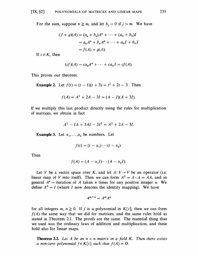
[IX, §2] POLYNOMIALS OF MATRICES AND LINEAR MAPS 235
For the sum, suppose n > m, and let bj = 0 if j > m. We have
= f(A) + g(A). If c E K, then
(cf)(A) = canAn + ... + cao1 = cf(A).
This proves our theorem.
Example 2. Let f(t) = (t - 1)(t + 3) = t2 + 2t - 3. Then
f(A) = A 2 + 2A - 31 = (A - 1)(A + 31).
If we multiply this last product directly using the rules for multiplication of matrices, we obtain in fact
A2 - 1A + 3A1 - 312 = A2 + 2A - 31.
Example 3. Let a l , ... ,an be numbers. Let
Then
Let V be a vector space over K, and let A: V ---+ V be an operator (i.e. linear map of V into itself). Then we can form A 2 = A 0 A = AA, and in general An = iteration of A taken n times for any positive integer n. We define A O = 1 (where I now denotes the identity mapping). We have
for all integers m, n > O. If f is a polynomial in K[t], then we can form f(A) the same way that we did for matrices, and the same rules hold as stated in Theorem 2.1. The proofs are the same. The essential thing that we used was the ordinary laws of addition and multiplication, and these hold also for linear maps.
Theorem 2.2. Let A be an n x n matrix in a field K. Then there exists a non-zero polynomial f E K[t] such that f(A) = O.
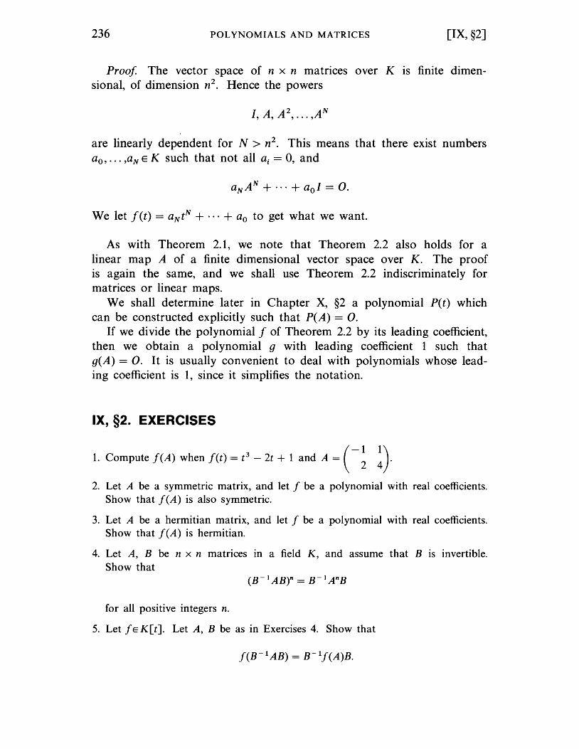
236 POLYNOMIALS AND MATRICES [IX, §2]
Proof The vector space of n x n matrices over K IS finite dimensional, of dimension n2
• Hence the powers
are linearly dependent for N > n2• This means that there exist numbers
ao, ... ,aN E K such that not all ai = 0, and
We let f(t) = aNtN + ... + ao to get what we want.
As with Theorem 2.1, we note that Theorem 2.2 also holds for a linear map A of a finite dimensional vector space over K. The proof is again the same, and we shall use Theorem 2.2 indiscriminately for matrices or linear maps.
We shall determine later in Chapter X, §2 a polynomial P(t) which can be constructed explicitly such that P(A) = O.
If we divide the polynomial f of Theorem 2.2 by its leading coefficient, then we obtain a polynomial g with leading coefficient 1 such that g(A) = O. It is usually convenient to deal with polynomials whose leading coefficient is 1, since it simplifies the notation.
IX, §2. EXERCISES
1. Compute f(A) when f(t) = t3 - 2t + 1 and A = (- ~ ~}
2. Let A be a symmetric matrix, and let f be a polynomial with real coefficients. Show that f(A) is also symmetric.
3. Let A be a hermitian matrix, and let f be a polynomial with real coefficients. Show that f(A) is hermitian.
4. Let A, B be n x n matrices in a field K, and assume that B is invertible. Show that
for all positive integers n.
5. Let f E K[t]. Let A, B be as in Exercises 4. Show that
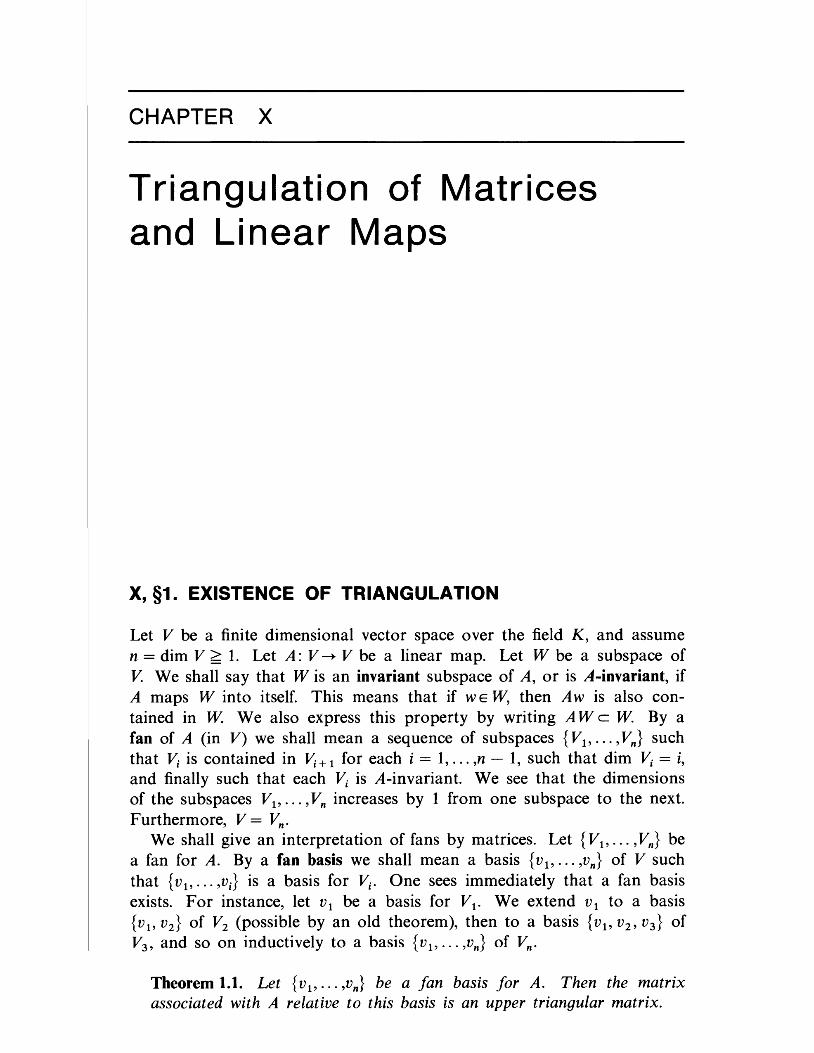
CHAPTER X
Triangulation of Matrices and Linear Maps
X, §1. EXISTENCE OF TRIANGULATION
Let V be a finite dimensional vector space over the field K, and assume n = dim V >1. Let A: V ---+ V be a linear map. Let W be a subspace of V. We shall say that W is an invariant subspace of A, or is A-invariant, if A maps W into itself. This means that if WE W, then Aw is also contained in W We also express this property by writing AWe W. By a fan of A (in V) we shall mean a sequence of subspaces {VI"'" Vn} such that Vi is contained in V; + 1 for each i = 1, ... ,n - 1, such that dim Vi = i, and finally such that each Vi is A-invariant. We see that the dimensions of the subspaces VI"'" Vn increases by 1 from one subspace to the next. Furthermore, V = Vn •
We shall give an interpretation of fans by matrices. Let {VI"'" Vn} be a fan for A. By a fan basis we shall mean a basis {VI"" ,Vn } of V such that {VI"" ,V;} is a basis for Vi' One sees immediately that a fan basis exists. F or instance, let V 1 be a basis for V l' We extend V 1 to a basis {VI' V2 } of V2 (possible by an old theorem), then to a basis {VI' V2 , V3 } of V3 , and so on inductively to a basis {VI"" ,Vn } of Vn -
Theorem 1.1. Let {VI"" ,Vn} be a fan basis for A. Then the matrix associated with A relative to this basis is an upper triangular matrix.
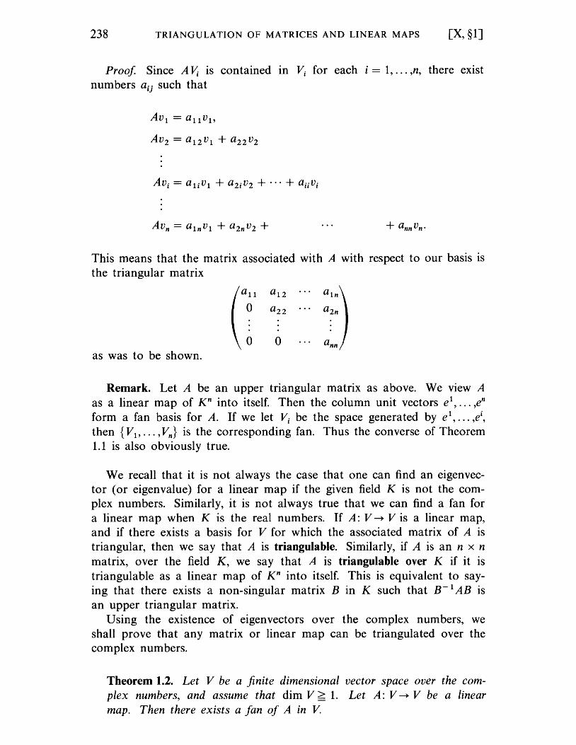
238 TRIANGULATION OF MATRICES AND LINEAR MAPS [X, §1]
Proof Since A ~ is contained In Vi for each i = 1, ... ,n, there exist numbers aij such that
This means that the matrix associated with A with respect to our basis is the triangular matrix
all a 1 2 a ln
o a22 a2n
as was to be shown.
Remark. Let A be an upper triangular matrix as above. We view A as a linear map of K n into itself. Then the column unit vectors e l
, ... ,en form a fan basis for A. If we let Vi be the space generated by e l
, ... ,ei,
then {VI' ... ' Vn} is the corresponding fan. Thus the converse of Theorem 1.1 is also obviously true.
We recall that it is not always the case that one can find an eigenvector (or eigenvalue) for a linear map if the given field K is not the complex numbers. Similarly, it is not always true that we can find a fan for a linear map when K is the real numbers. If A: V ---+ V is a linear map, and if there exists a basis for V for which the associated matrix of A is triangular, then we say that A is triangulable. Similarly, if A is an n x n matrix, over the field K, we say that A is triangulable over K if it is triangulable as a linear map of K n into itself. This is equivalent to saying that there exists a non-singular matrix B in K such that B- 1 AB is an upper triangular matrix.
Using the existence of eigenvectors over the complex numbers, we shall prove that any matrix or linear map can be triangulated over the complex numbers.
Theorem 1.2. Let V be a finite dimensional vector space over the complex numbers, and assume that dim V >1. Let A: V ---+ V be a linear map. Then there exists a fan of A in V.
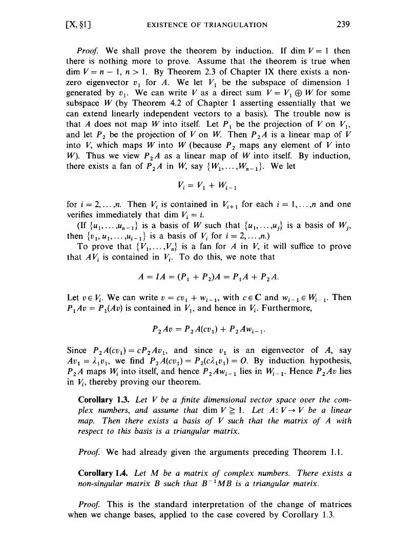
[X, §1] EXISTENCE OF TRIANGULATION 239
Proof We shall prove the theorem by induction. If dim V = 1 then there is nothing more to prove. Assume that the theorem is true when dim V = n - 1, n > 1. By Theorem 2.3 of Chapter IX there exists a nonzero eigenvector V 1 for A. We let V1 be the subspace of dimension 1 generated by V 1• We can write V as a direct sum V = V1 EB W for some subspace W (by Theorem 4.2 of Chapter I asserting essentially that we can extend linearly independent vectors to a basis). The trouble now is that A does not map W into itself. Let P 1 be the projection of V on V1 ,
and let P 2 be the projection of V on W. Then P 2 A is a linear map of V into V, which maps W into W (because P 2 maps any element of V into W). Thus we view P 2 A as a linear map of W into itself. By induction, there exists a fan of P 2 A in W, say {W1, ... ,Wn - 1}. We let
for i = 2, ... ,no Then Vi is contained in ~+ 1 for each i = 1, ... ,n and one verifies immediately that dim Vi = i.
(If {u 1, ... ,un - 1 } is a basis of W such that {u 1, ... ,uj } is a basis of Wj' then {v 1, u1, ..• 'U i - 1 } is a basis of Vi for i = 2, ... ,n.)
To prove that {V1, ... , Vn } is a fan for A in V, it will suffice to prove that AVi is contained in Vi. To do this, we note that
Let v E JIi. We can write v = CV 1 + Wi-l, with C E C and Wi-l E Wi-I. Then P1Av = P1(Av) is contained in VI, and hence in J!i. Furthermore,
Since P2A(cvt) = cP2 Av1, and since VI is an eigenvector of A, say AVI = A1V1, we find P2A(cv l) = P2(CAIV1) = O. By induction hypothesis, P2A maps Wi into itself, and hence P2Awi-1 lies in Wi-I. Hence P2Av lies in JIi, thereby proving our theorem.
Corollary 1.3. Let V be a finite dimensional vector space over the complex numbers, and assume that dim V >1. Let A: V ~ V be a linear map. Then there exists a basis of V such that the matrix of A with respect to this basis is a triangular matrix.
Proof We had already given the arguments preceding Theorem 1.1.
Corollary 1.4. Let M be a matrix of complex numbers. There exists a non-singular matrix B such that B- 1 M B is a triangular matrix.
Proof This is the standard interpretation of the change of matrices when we change bases, applied to the case covered by Corollary 1.3.
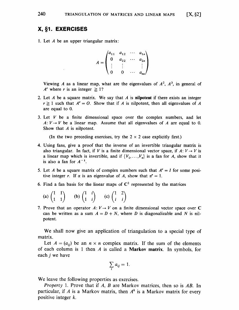
240 TRIANGULATION OF MATRICES AND LINEAR MAPS [X, §2]
X, §1. EXERCISES
1. Let A be an upper triangular matrix:
Viewing A as a linear map, what are the eigenvalues of A 2, A 3, in general of Ar where r is an integer ~ I?
2. Let A be a square matrix. We say that A is nilpotent if there exists an integer r ~ 1 such that A r = O. Show that if A is nilpotent, then all eigenvalues of A are equal to o.
3. Let V be a finite dimensional space over the complex numbers, and let A: V ---. V be a linear map. Assume that all eigenvalues of A are equal to o. Show that A is nilpotent.
(In the two preceding exercises, try the 2 x 2 case explicitly first.)
4. Using fans, give a proof that the inverse of an invertible triangular matrix is also triangular. In fact, if V is a finite dimensional vector space, if A: V --+ V is a linear map which is invertible, and if {Vi' ... ,Vn} is a fan for A, show that it is also a fan for A-i.
5. Let A be a square matrix of complex numbers such that Ar = I for some positive integer r. If tX is an eigenvalue of A, show that tXr = 1.
6. Find a fan basis for the linear maps of C2 represented by the matrices
(1 11) (a) 1 (b) G :) (c) G ~) 7. Prove that an operator A: V --+ V on a finite dimensional vector space over C
can be written as a sum A = D + N, where D is diagonalizable and N is nilpotent.
We shall now give an application of triangulation to a special type of matrix.
Let A = (aij) be an n x n complex matrix. If the sum of the elements of each column is 1 then A is called a Markov matrix. In symbols, for each j we have
We leave the following properties as exercises. Property 1. Prove that if A, B are Markov matrices, then so is AB. In
particular, if A is a Markov matrix, then Ak is a Markov matrix for every positive integer k.
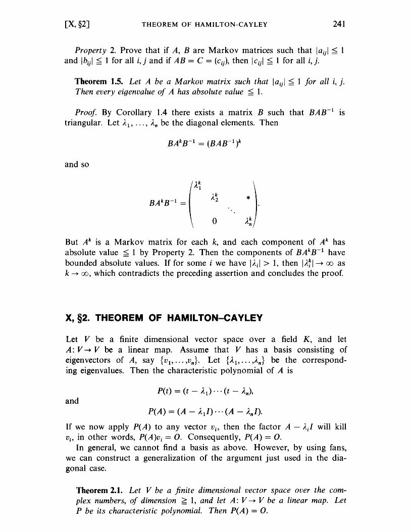
[X, §2] THEOREM OF HAMILTON-CAYLEY 241
Property 2. Prove that if A, B are Markov matrices such that laijl < 1 and Ibijl < 1 for all i, j and if AB = C = (c ij ), then ICijl < 1 for all i, j.
Theorem 1.5. Let A be a Markov matrix such that laijl < 1 for all i, j. Then every eigenvalue of A has absolute value < 1.
Proof By Corollary 1.4 there exists a matrix B such that BAB- 1 IS
triangular. Let A1 , ••• , An be the diagonal elements. Then
and so
o
But Ak is a Markov matrix for each k, and each component of Ak has absolute value < 1 by Property 2. Then the components of BAkB- 1 have bounded absolute values. If for some i we have IAil > 1, then IA~I---+ 00 as k ~ 00, which contradicts the preceding assertion and concludes the proof.
X, §2. THEOREM OF HAMIL TON-CA YLEY
Let V be a finite dimensional vector space over a field K, and let A: V ---+ V be a linear map. Assume that V has a basis consisting of eigenvectors of A, say {v 1, ••• ,vn}. Let {A 1, ••• ,An} be the corresponding eigenvalues. Then the characteristic polynomial of A is
P(t) = (t - A1) ••• (t - An), and
P(A) = (A - All)··· (A - AnI).
If we now apply P(A) to any vector Vi' then the factor A - Ail will kill Vi' in other words, P(A)Vi = o. Consequently, P(A) = O.
In general, we cannot find a basis as above. However, by using fans, we can construct a generalization of the argument just used in the diagonal case.
Theorem 2.1. Let V be a finite dimensional vector space over the complex numbers, of dimension > 1, and let A: V ---+ V be a linear map. Let P be its characteristic polynomial. Then P(A) = o.
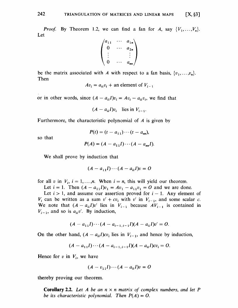
242 TRIANGULATION OF MATRICES AND LINEAR MAPS [X, §3]
Proof By Theorem 1.2, we can find a fan for A, say {V1 , ••• , Vn }.
Let
be the matrix associated with A with respect to a fan basis, {v 1, ••• ,vn}.
Then AVi = aUvi + an element of Vi- 1
or in other words, since (A - aiiI)vi = AVi - aiivi, we find that
(A - auI)vi lies in Vi - 1.
Furthermore, the characteristic polynomial of A is given by
so that
We shall prove by induction that
for all v in Vi' i = 1, ... ,no When i = n, this will yield our theorem. Let i = 1. Then (A - all I)V1 = AV1 - all V1 = 0 and we are done. Let i > 1, and assume our assertion proved for i - 1. Any element of
Vi can be written as a sum v' + CVi with v' in Vi - 1, and some scalar c. We note that (A - aiiI)v' lies in Vi- 1 because AVi- 1 is contained in Vi- 1, and so is auv'. By induction,
(A - a11 I)··· (A - ai-1,i-1I)(A - aiiI)v' = O.
On the other hand, (A - auI)cvi lies in Vi- 1, and hence by induction,
Hence for v in Vi' we have
thereby proving our theorem.
Corollary 2.2. Let A be an n x n matrix of complex numbers, and let P be its characteristic polynomial. Then peA) = o.

[X, §3] DIAGONALIZATION OF UNITARY MAPS 243
Proof We VIew A as a linear map of cn into itself, and apply the theorem.
Corollary 2.3. Let V be a finite dimensional vector space over the field K, and let A: V ~ V be a linear map. Let P be the characteristic polynomial of A. Then peA) = o.
Proof Take a basis of V, and let M be the matrix representing A with respect to this basis. Then PM = P A' and it suffices to prove that PM(M) = O. But we can apply Theorem 2.1 to conclude the proof.
Remark. One can base a proof of Theorem 2.1 on a continuity argument. Given a complex matrix A, one can, by various methods into which we don't go here, prove that there exist matrices Z of the same size as A, lying arbitrarily close to A (i.e. each component of Z is close to the corresponding component of A) such that Pz has all its roots of multiplicity 1. In fact, the complex polynomials having roots of multiplicity > 1 are thinly distributed among all polynomials. Now, if Z is as above, then the linear map it represents is diagonalizable (because Z has distinct eigenvalues), and hence Pz{Z) = 0 trivially, as noted at the beginning of this section. However, Pz(Z) approaches P A(A) as Z approaches A. Hence P A(A) = o.
X, §3. DIAGONALIZATION OF UNITARY MAPS
Using the methods of this chapter, we shall give a new proof for the following theorem, already proved in Chapter VIII.
Theorem 3.1. Let V be a finite dimensil)nal vector space over the complex numbers, and let dim V >1. Assume given a positive definite hermitian product on V. Let A: V ~ V be a unitary map. Then there exists an orthogonal basis of V consisting of eigenvectors of A.
Proof First observe that if w is an eigenvector for A, with eigenvalue A, then A w = A w, and A i= 0 beca use A preserves length.
By Theorem 1.2, we can find a fan for A, say {V1 , ... , Vn}. Let {v1, ... ,vn} be a fan basis. We can use the Gram-Schmidt orthogonalization process to orthogonalize it. We recall the process:
244 TRIANGULATION OF MATRICES AND LINEAR MAPS [X, §3]
From this construction, we see that {V'l' ... ,v~} is an orthogonal basis which is again a fan basis, because {V'l' ... ,va is a basis of the same space Vi as {v l , ... ,vJ. Dividing each v~ by its norm we obtain a fan basis {w l , ... ,wn} which is orthonormal. We contend that each Wi is an eigenvector for A. We proceed by induction. Since AWl is contained in Vl' there exist a scalar Al such that AWl = Alw l , so that W l is an eigenvector, and Al i= o. Assume that we have already proved that W l , •.. ,Wi-l are eigenvectors with non-zero eigenvalues. There exist scalars c l' ... 'Ci such that
Since A preserves perpendicularity, AWi is perpendicular to AWk for every k < i. But AWk = Ak Wk. Hence AWi is perpendicular to Wk itself, and hence Ck = O. Hence AWi = CiWi' and Ci i= 0 because A preserves length. We can thus go from 1 to n to prove our theorem.
Corollary 3.2. Let A be a complex unitary matrix. Then there exists a unitary matrix U such that U - 1 A U is a diagonal matrix.
Proof Let {e l, ... ,en} = 81 be the standard orthonormal basis of cn,
and let {w l , ... ,wn} = 81' be an orthonormal basis which diagonalizes A, viewed as a linear map of cn into itself. Let
Then U is unitary (cf. Exercise 5 of Chapter VII, §3), and if M' IS the matrix of A relative to the basis 81', then
M' = U-lAU.
This proves the Corollary.
X, §3. EXERCISES
1. Let A be a complex unitary matrix. Show that each eigenvalue of A can be written ei8 with some real O.
2. Let A be a complex unitary matrix. Show that there exists a diagonal matrix B and a complex unitary matrix U such A = U- 1 BU.
CHAPTER XI
Polynomials and Primary Decomposition
XI, §1. THE EUCLIDEAN ALGORITHM
We have already defined polynomials, and their degree, in Chapter IX. In this chapter, we deal with the other standard properties of polynomials. The basic one is the Euclidean algorithm, or long division, taught (presumably) in all elementary schools.
Theorem 1.1. Let J, g be polynomials over the field K, i.e. polynomials in K[t], and assume deg g > O. Then there exist polynomials q, r in K[t] such that
J(t) = q(t)g(t) + ret),
and deg r < deg g. The polynomials q, r are uniquely determined by these conditions.
Proof Let m = deg g > o. Write
J(t) = antn + ... + ao,
get) = bmtm + ... + bo,
with bm i= o. If n < m, let q = 0, r = J. If n > m, let
246 POLYNOMIALS AND PRIMARY DECOMPOSITION [XI, §1]
(This is the first step in the process of long division.) Then degfl < degf. Continuing in this way, or more formally by induction on n, we can find polynomials q1' r such that
with deg r < deg g. Then
f(t) = anb;;; 1tn -mg(t) + f1 (t)
= anb;;; 1tn - mg(t) + q 1 (t)g(t) + r(t)
= (an b;;; 1 tn - m + q 1 )g( t) + r( t),
and we have consequently expressed our polynomial in the desired form. To prove the uniqueness, suppose that
with deg r 1 < deg g and deg r2 < deg g. Then
The degree of the left-hand side is either > deg g, or the left-hand side is equal to O. The degree of the right-hand side is either < deg g, or the right-hand side is equal to O. Hence the only possibility is that they are both 0, whence
and
as was to be shown.
Corollary 1.2. Let f be a non-zero polynomial in K[tJ. Let a E K be such that f(a) = O. Then there exists a polynomial q(t) in K[t] such that
f(t) = (t - a)q(t).
Proof We can write
f(t) = q(t)(t - a) + r(t),
where deg r < deg(t - a). But deg(t - a) = 1. Hence r is constant. Since
o = f(a) = q(a)(a - a) + r(a) = r(a),
it follows that r = 0, as desired.
[XI, §1] THE EUCLIDEAN ALGORITHM 247
Corollary 1.3. Let K be a field such that every non-constant polynomial in K[t] has a root in K. Let f be such a polynomial. Then there exist elements ex l , ... ,exn E K and c E K such that
Proof In Corollary 1.2, observe that deg q = degf - 1. Let ex = ex l in Corollary 1.2. By assumption, if q is not constant, we can find a root ex 2
of q, and thus write
Proceeding inductively, we keep on going until qn is constant.
Assuming as we do that the complex numbers satisfy the hypothesis of Corollary 1.3, we see that we have proved the existence of a factorization of a polynomial over the complex numbers into factors of degree 1. The uniqueness will be proved in the next section.
Corollary 1.4. Let f be a polynomial of degree n in K[t]. There are at most n roots of f in K.
Proof Otherwise, if m > n, and ex l , ... ,exm are distinct roots of f in K, then
for some polynomial g, whence degf > m, contradiction.
XI, §1. EXERCISES
1. In each of the following cases, write f = qg + r with deg r < deg g. (a) f (t) = t2
- 2t + 1, g( t) = t - 1 (b) f(t) = t 3 + t - 1, g(t) = t2 + 1 (c) f(t) = t 3 + t, g(t) = t ( d) f (t) = t 3
- 1, g( t) = t - 1
2. If f(t) has integer coefficients, and if g(t) has integer coefficients and leading coefficient 1, show that when we express f = qg + r with deg r < deg g, the polynomials q and r also have integer coefficients.
3. Using the intermediate value theorem of calculus, show that every polynomial of odd degree over the real n urn bers has a root in the real n urn bers.
4. Let f(t) = t" + ... + ao be a polynomial with complex coefficients, of degree n, and let rJ. be a root. Show that 1rJ.1 ~ n· maxi lad. [Hint: Write -rJ." = a"_lrJ."-l + ... + ao. If 1rJ.1 > n· maxi lail, divide by rJ." and take the absolute value, together with a simple estimate to get a contradiction.]
248 POLYNOMIALS AND PRIMARY DECOMPOSITION [XI, §2]
XI, §2. GREATEST COMMON DIVISOR
We shall define a notion which bears to the set of polynomials K[t] the same relation as a subspace bears to a vector space.
By an ideal of K[t], or a polynomial ideal, or more briefly an ideal we shall mean a subset J of K[t] satisfying the following conditions.
The zero polynomial is in J. If f, g are in J, then f + g is in J. If f is in J, and g is an arbitrary polynomial, then gf is in J.
From this last condition, we note that if C E K, and f is in J, then cf is also in J. Thus an ideal may be viewed as a vector space over K. But it is more than that, in view of the fact that it can stand multiplication by arbitrary elements of K[t], not only constants.
Example 1. Let f1' ... ,fn be polynomials in K[t]. Let J be the set of all polynomials which can be written in the form
with some gi E K[t]. Then J is an ideal. Indeed, if
with hj E K[t], then
also lies in J. Also, 0 = Of1 + ... + Ofn lies in J. If f is an arbitrary polynomial in K[t], then
is also in J. Thus all our conditions are satisfied.
The ideal J in Example 1 is said to be generated by f1"" ,fn' and we say that f1"" ,fn are a set of generators.
We note that each fi lies in the ideal J of Example 1. For instance,
Example 2. The single element 0 is an ideal. Also, K[t] itself is an ideal. We note that 1 is a generator for K[t], which is called the unit ideal.
[XI, §2] GREATEST COMMON DIVISOR 249
Example 3. Consider the ideal generated by the two polynomials t - 1 and t - 2. We contend that it is the unit ideal. Namely,
(t - 1) - (t - 2) = 1
IS In it. Thus it may happen that we are given several generators for an ideal, and still we may find a single generator for it. We shall describe more precisely the situation in the subsequent theorems.
Theorem 2.1. Let J be an ideal of K[t]. Then there exists a polynomial g which is a generator of J.
Proof Suppose that J is not the zero ideal. Let g be a polynomial in J which is not 0, and is of smallest degree. We assert that g is a generator for J. Let f be any element of J. By the Euclidean algorithm, we can find polynomials q, r such that
f= qg + r
with deg r < deg g. Then r = f - qg, and by the definition of an ideal, it follows that r also lies in J. Since deg r < deg g, we must have r = O. Hence f = qg, and g is a generator for J, as desired.
Remark. Let gl be a non-zero generator for an ideal J, and let g2 also be a generator. Then there exists a polynomial q such that gl = qg2· Since
it follows that deg g2 < deg gl. By symmetry, we must have
Hence q is constant. We can write
with some constant c. Write
with an =1= O. Take b = a; 1. Then bg 2 is also a generator of J, and its leading coefficient is equal to 1. Thus we can always find a generator for an ideal (=1= 0) whose leading coefficient is 1. It is furthermore clear that this generator is uniquely determined.
250 POLYNOMIALS AND PRIMARY DECOMPOSITION [XI, §2]
Let I, g be non-zero polynomials. We shall say that g divides I, and write g I I, if there exists a polynomial q such that I = gq. Let 11' 12 be polynomials i= O. By a greatest common divisor of 11, 12 we shall mean a polynomial g such that g divides 11 and 12' and furthermore, if h divides 11 and 12' then h divides g.
Theorem 2.2. Let 11' 12 be non-zero polynomials in K[t]. Let g be a generator lor the ideal generated by 11' 12. Then g is a greatest common divisor 01 11 and 12.
Proof. Since 11 lies in the ideal generated by 11' 12' there exists a polynomial q 1 such that
whence g divides 11. Similarly, g divides 12. Let h be a polynomial dividing both 11 and 12. Write
and
with some polynomials hl and h2. Since g is in the ideal generated by 11,/2, there are polynomials gl' g2 such that g = gl/1 + g2/2' whence
Consequently h divides g, and our theorem is proved.
Remark 1. The greatest common divisor is determined up to a nonzero constant multiple. If we select a greatest common divisor with leading coefficient 1, then it is uniquely determined.
Remark 2. Exactly the same proof applies when we have more than two polynomials. For instance, if lb ... ,In are non-zero polynomials, and if g is a generator for the ideal generated by 11' ... ' In then g is a greatest common divisor of /1'··· ,In.
Polynomials 11' ... ,In whose greatest common divisor is 1 are said to be relatively prime.
XI, §2. EXERCISES
1. Show that tn - 1 is divisible by t - 1.
2. Show that t4 + 4 can be factored as a product of polynomials of degree 2 with integer coefficients.
[XI, §3] UNIQUE FACTORIZATION 251
3. If n is odd, find the quotient of tn + 1 by t + 1.
4. Let A be an n x n matrix over a field K, and let J be the set of all polynomials f(t) in K[tJ such that f(A) = o. Show that J is an ideal.
XI, §3. UNIQUE FACTORIZATION
A polynomial p in K[t] will be said to be irreducible (over K) if it is of degree > 1, and if, given a factorization p = fg with f, g E K[t], then degf or deg g = 0 (i.e. one of f, g is constant). Thus, up to a non-zero constant factor, the only divisors of pare p itself, and 1.
Example 1. The only irreducible polynomials over the complex numbers are the polynomials of degree 1, i.e. non-zero constant multiples of polynomials of type t - a, with a E C.
Example 2. The polynomial t 2 + 1 is irreducible over R.
Theorem 3.1. Every polynomial in K[t] of degree > 1 can be expressed as a product P1' ... ,Pm of irreducible polynomials. In such a product, the polynomials P1' ... ,Pm are uniquely determined, up to a rearrangement, and up to non-zero constant factors.
Proof. We first prove the existence of the factorization into a product of irreducible polynomials. Let f be in K[tJ, of degree > 1. If f is irreducible, we are done. Otherwise, we can write
f= gh,
where deg g < deg f and deg h < deg f. If g, h are irreducible, we are done. Otherwise, we further factor g and h into polynomials of lower degree. We cannot continue this process indefinitely, and hence there exists a factorization for f. (We can obviously phrase the proof as an induction.)
We must now prove uniqueness. We need a lemma.
Lemma 3.2. Let p be irreducible in K[t]. Let f, g E K[t] be non-zero polynomials, and assume p divides fg. Then p divides f or p divides g.
Proof. Assume that p does not divide f. Then the greatest common divisor of p and f is 1, and there exist polynomials hi' h2 in K[tJ such that
252 POLYNOMIALS AND PRIMARY DECOMPOSITION [XI, §3]
(We use Theorem 2.2.) Multiplying by g yields
But fg = ph3 for some h3' whence
and p divides g, as was to be shown.
The lemma will be applied when p divides a product of irreducible polynomials q 1 ..• qs' In that case, p divides q 1 or P divides q2'" qs· Hence there exists a constant c such that p = cq l' or P divides q2'" qs. In the ,latter case, we can proceed inductively, and we conclude that in any case, there exists some i such that p and q i differ by a constant factor.
Suppose now that we have two products of irreducible polynomials
After renumbering the qi' we may assume that Pi = c1ql for some constant c1 • Cancelling ql' we obtain
Repeating our argument inductively, we conclude that there exist constants Ci such that Pi = ciqi for all i, after making a possible permutation of q l' ... ,qs. This proves the desired uniqueness.
Corollary 3.3. Let f be a polynomial in K[t] of degree > 1. Then f has a factorization f = CPl'" Ps' where Pi"" ,Ps are irreducible polynomials with leading coefficient 1 , uniquely determined up to a permutation.
Corollary 3.4. Let f be a polynomial in C[t], of degree > 1. Then f has a factorization
with ai E C and c E C. The factors t - ai are uniquely determined up to a permutation.
We shall deal mostly with polynomials having leading coefficient 1. Let f be such a polynomial of degree > 1. Let Pi"" ,Pr be the distinct irreducible polynomials (with leading coefficient 1) occurring in its factorization. Then we can express f as a product
[XI, §3] UNIQUE FACTORIZATION 253
where i1, ••• ,ir are positive integers, uniquely determined by Pl'··· ,Pro This factorization will be called a normalized factorization for f. In particular, over the complex numbers, we can write
A polynomial with leading coefficient 1 is sometimes called monic. If p is irreducible, and f = pmg, where p does not divide g, and m is an
integer > 0, then we say that m is the multiplicity of p in f. (We define pO to be 1.) We denote this multiplicity by ordpf, and also call it the order of f at p.
If rx is a root of f, and
f(t) = (t - rx)mg(t),
with g(rx) i= 0, then t - rx does not divide g(t), and m is the multiplicity of t - rx in f. We also say that m is the multiplicity of rx in f.
There is an easy test for m > 1 in terms of the derivative. Let f(t) = antn + ... + ao be a polynomial. Define its (formal) deriva
tive to be
Then we have the following statements, whose proofs are left as exercises.
(a) If f, g are polynomials, then
(f + g)' = f' + g'. Also
(fg), = f'g + fg'·
If c is constant, then (cf)' = cf'.
(b) Let rx be a root of f and assume degf > 1. Show that the multiplicity of rx in f is > 1 if and only if f'(rx) = 0. Hence if f'(rx) i= 0, the multiplicity of rx is 1.
XI, §3. EXERCISES
1. Let f be a polynomial of degree 2 over a field K. Show that either f is irreducible over K, or f has a factorization into linear factors over K.
2. Let f be a polynomial of degree 3 over a field K. If f is not irreducible over K, show that f has a root in K.
254 POLYNOMIALS AND PRIMARY DECOMPOSITION [XI, §3]
3. Let f(t) be an irreducible polynomial with leading coefficient lover the real numbers. Assume degf = 2. Show that f(t) can be written in the form
f(t) = (t - a)2 + b2
with some a, bE Rand b i= O. Conversely, prove that any such polynomial is irreducible over R.
4. Let f be a polynomial with complex coefficients, say
Define its complex conjugate,
by taking the complex conjugate of each coefficient. Show that if f, g are in C[t], then
(f + g) = J + g, (fg) = Jg,
and if P E C, then (Pf) = pI 5. Let f(t) be a polynomial with real coefficients. Let (X be a root of f, which is
complex but not real. Show that a is also a root of f.
6. Terminology being as in Exercise 5, show that the multiplicity of (X in f is the same as that of a.
7. Let A be an n x n matrix in a field K. Let J be the set of polynomials f in K[t] such that f(A) = O. Show that J is an ideal. The monic generator of J is called the minimal polynomial of A over K. A similar definition is made if A is a linear map of a finite dimensional vector space V into itself.
8. Let V be a finite dimensional space over K. Let A: V ~ V be a linear map. Let f be its minimal polynomial. If A can be diagonalized (i.e. if there exists a basis of V consisting of eigenvectors of A), show that the minimal polynomial is equal to the product
where (Xl"" '(Xr are the distinct eigenvalues of A.
9. Show that the following polynomials have no multiple roots in C. (a) t4 + t (b) t 5
- 5t + 1 (c) any polynomial t2 + bt + c if b, c are numbers such that b2
- 4c is not O.
10. Show that the polynomial tn - 1 has no multiple roots in C. Can you deter
mine all the roots and give its factorization into factors of degree I?
[XI, §4] THE DECOMPOSITION OF A VECTOR SPACE 255
11. Let I, g be polynomials in K[tJ, and assume that they are relatively prime. Show that one can find polynomials 11' gl such that the determinant
is equal to 1.
12. Let 11' 12' 13 be polynomials in K[t] and assume that they generate the unit ideal. Show that one can find polynomials Iij in K[tJ such that the determinant
is equal to 1.
11 12 13
121 122 123
131 132 133
13. Let rx be a complex number, and let J be the set of all polynomials I(t) in K[tJ such that I(rx) = O. Show that J is an ideal. Assume that J is not the zero ideal. Show that the monic generator of J is irreducible.
14. Let I, g be two polynomials, written in the form
and
where iv, jv are integers ~ 0, and P l' ... 'Pr are distinct irreducible polynomials. (a) Show that the greatest common divisor of I and g can be expressed as a
product p~l ... p~r where k l' ... ,kr are integers ~ O. Express kv in terms of iv and jv·
(b) Define the least common mUltiple of polynomials, and express the least common multiple of I and g as a product p~l ... p~r with integers kv ~ O. Express kv in terms of iv and j v .
15. Give the greatest common divisor and least common multiple of the following pairs of polynomials: (a) (t - 2)3(t - 3)4(t - i) and (t - 1)(t - 2)(t - 3)3 (b) (t 2 + 1)(t2
- 1) and (t + i)3(t3 - 1)
XI, §4. APPLICATION TO THE DECOMPOSITION OF A VECTOR SPACE
Let V be a vector space over the field K, and let A: V ~ V be an operator of V. Let W be a subspace of V. We shall say that W is an invariant subspace under A if Aw lies in W for each w in W, i.e. if A W is contained in W.
256 POLYNOMIALS AND PRIMARY DECOMPOSITION [XI, §4]
Example 1. Let Vi be a non-zero eigenvector of A, and let Vi be the I-dimensional space generated by Vi. Then Vi is an invariant subspace under A.
Example 2. Let A be an eigenvalue of A, and let V;. be the subspace of V consisting of all V E V such that Av = Av. Then V;. is an invariant subspace under A, called the eigenspace of A.
Example 3. Let f(t) E K[t] be a polynomial, and let W be the kernel of f(A). Then W is an invariant subspace under A.
Proof. Suppose that f(A)w = O. Since tf(t) = f(t)t, we get
Af(A) = f(A)A, whence
f(A)(Aw) = f(A)Aw = Af(A)w = O.
Thus Aw is also in the kernel of f(A), thereby proving our assertion.
Remark in general that for any two polynomials f, g we have
f(A)g(A) = g(A)f(A)
because f(t)g(t) = g(t)f(t). We use this frequently in the sequel. We shall now describe how the factorization of a polynomial into two
factors whose greatest common divisor is 1, gives rise to a decomposition of the vector space V into a direct sum of invariant subspaces.
Theorem 4.1. Let f(t) E K[t] be a polynomial, and suppose that f = flf2' where fl' f2 are polynomials of degree > 1, and greatest common divisor equal to 1. Let A: V ---+ V be an operator. Assume that f(A) = O. Let
Wi = kernel of fl (A) and
Then V is the direct sum of WI and W2.
Proof By assumption, there exist polynomials gl' g2 such that
Hence
[XI, §4] THE DECOMPOSITION OF A VECTOR SPACE 257
Let v E V. Then
The first term in this sum belongs to W 2 , because
Similarly, the second term in this sum belongs to W 1• Thus V is the sum of W 1 and W2 •
To show that this sum is direct, we must prove that an expression
with W 1 E W 1 and W2 E W2 , is uniquely determined by v. Applying g1(A)f1(A) to this sum, we find
because f1(A)w 1 = O. Applying the expression (*) to W 2 itself, we find
because f2(A)W2 = O. Consequently
w2 = g 1 (A)f1 (A)v,
and hence W2 is uniquely determined. Similarly, W 1 = g2(A)f2(A)v is uniquely determined, and the sum is therefore direct. This proves our theorem.
Theorem 4.1 applies as well when f is expressed as a product of several factors. We state the result over the complex numbers.
Theorem 4.2. Let V be a vector space over C, and let A: V ---+ V be an operator. Let P(t) be a polynomial such that P(A) = 0, and let
be its factorization, the rx l' ... ,rxr being the distinct roots. Let Wi be the kernel of (A - rxiI)mi. Then V is the direct sum of the subspaces
W1,··· ,Wr •
258 POLYNOMIALS AND PRIMARY DECOMPOSITION [XI, §4]
Proof The proof can be done by induction, splitting off the factors (t - ai)mt, (t - a 2 )m\ ... ,one by one. Let
Wi = Kernel of (A - aiI)m 1,
W= Kernel of (A - a 2 I)m2···(A - arI)mr.
By Theorem 4.1 we obtain a direct sum decomposition V = Wi EB W Now, inductively, we can assume that W is expressed as a direct sum
where Wj (j = 2, ... ,r) is the kernel of (A - ajI)m j in W. Then
is a direct sum. We still have to prove that Wj (j = 2, ... ,r) is the kernel of (A - ajI)m j in V. Let
be an element of V, with WiE Wi' and such that v IS In the kernel of (A - ajI)m j
• Then in particular, v is in the kernel of
whence v must be in W, and consequently Wi = o. Since v lies in W, we can now conclude that v = Wj because W is the direct sum of W 2 , .•• , Wr.
Example 4. Differential equations. Let V be the space of (infinitely differentiable) solutions of the differential equation
with constant complex coefficients ai •
Theorem 4.3 Let
P( ) n n-i t = t + an - 1 t + ... + ao·
Factor pet) as in Theorem 5.2
[XI, §4] THE DECOMPOSITION OF A VECTOR SPACE 259
Then V is the direct sum of the spaces of solutions of the differential equations
for i = 1, ... ,r.
Proof This is merely a direct application of Theorem 4.2.
Thus the study of the original differential equation is reduced to the study of the much simpler equation
The solutions of this equation are easily found.
Theorem 4.4 Let rx be a complex number. Let W be the space of solutions of the differential equation
Then W is the space generated by the functions
eIXt teIXt tm - 1 eIXt , , ... ,
and these functions form a basis for this space, which therefore has dimension m.
Proof For any complex rx we have
(The proof is a simple induction.) Consequently, f lies in the kernel of (D - rxI)m if and only if
The only functions whose m-th derivative is 0 are the polynomials of degree < m - 1. Hence the space of solutions of (D - rxI)mf = 0 is the space generated by the functions
eIXt teIXt tm - 1 eIXt , , ... , .
Finally these functions are linearly independent. Suppose we have a linear relation
260 POLYNOMIALS AND PRIMARY DECOMPOSITION [XI, §5]
for all t, with constants co, ... 'Cm - l' Let
Then Q(t) is a non-zero polynomial, and we have
Q(t)ecxt = 0 for all t.
But ecxt i= 0 for all t so Q(t) = 0 for all t. Since Q is a polynomial, we must have Ci = 0 for i = 0, ... ,m - 1 thus concluding the proof.
XI, §4. EXERCISES
1. In Theorem 4.1 show that image of 11 (A) = kernel of I2{A).
2. Let A: V --+ V be an operator, and V finite dimensional. Suppose that A 3 = A. Show that V is the direct sum
where Vo = Ker A, V1 is the {+ I)-eigenspace of A, and V -1 is the {-I)-eigenspace of A.
3. Let A: V --+ V be an operator, and V finite dimensional. Suppose that the characteristic polynomial of A has the factorization
where ~1"" '~n are distinct elements of the field K. Show that V has a basis consisting of eigenvectors for A.
XI, §5. SCHUR'S LEMMA
Let V be a vector space over K, and let S be a set of operators of V. Let W be a subspace of V. We shall say that W is an S-invariant subspace if BW is contained in W for all B in S. We shall say that V is a simple S-space if V i= {O} and if the only S-invariant subspaces are V itself and the zero subspace.
Remark 1. Let A: V -+ V be an operator such that AB = BA for all BE S. Then the image and kernel of A are S-invariant subspaces of V.
[XI, §5] SCHUR'S LEMMA 261
Proof. Let w be in the image of A, say w = Av with some VEV. Then Bw = BAv = ABv. This shows that Bw is also in the image of A, and hence that the image of A is S-invariant. Let u be in the kernel of A. Then ABu = BAu = O. Hence Bu is also in the kernel, which is therefore an S-invariant subspace.
Remark 2. Let S be as above, and let A: V -+ V be an operator. Assume that AB = BA for all BE S. If f is a polynomial in K[t], then f(A)B = Bf(A) for all BE S.
Prove this as a simple exercise.
Theorem 5.1. Let V be a vector space over K, and let S be a set of operators of V. Assume that V is a simple S-space. Let A: V -+ V be a linear map such that AB = BA for all B in S. Then either A is invertible or A is the zero map.
Proof. Assume A i= O. By Remark 1, the kernel of A is {O}, and its image is all of V. Hence A is invertible.
Theorem 5.2. Let V be a finite dimensional vector space over the complex numbers. Let S be a set of operators of V, and assume that V is a simple S-space. Let A: V -+ V be a linear map such that AB = BA for all B in S. Then there exists a number A such that A = AI.
Proof. Let J be the ideal of polynomials f in C[t] such that f(A) = O. Let g be a generator for this ideal, with leading coefficient 1. Then g i= o. We contend that g is irreducible. Otherwise, we can write g = h1h2 with polynomials h1' h2 of degrees < deg g. Consequently h1(A) i= O. By Theorem 5.1, and Remarks 1, 2 we conclude that h1(A) is invertible. Similarly, h2(A) is invertible. Hence h1 (A)h2(A) is invertible, an impossibility which proves that g must be irreducible. But the only irreducible polynomials over the complex numbers are of degree 1, and hence g(t) = t - A for some A E C. Since g(A) = 0, we conclude that A - AI = 0, whence A = AI, as was to be shown.
XI, §5. EXERCISES
1. Let V be a finite dimensional vector space over the field K, and let S be the set of all linear maps of V into itself. Show that V is a simple S-space.
2. Let V = R 2, let S consist of the matrix (~ ~) viewed as linear map of V into
itself. Here, a is a fixed non-zero real number. Determine all S-invariant subspaces of V.
262 POLYNOMIALS AND PRIMARY DECOMPOSITION [XI, §6]
3. Let V be a vector space over the field K, and let {v l' ... ,vn } be a basis of V. For each permutation (f of {I, ... ,n} let Au: V --+ V be the linear map such that
(a) Show that for any two permutations (f, ! we have
and Aid = I. (b) Show that the subspace generated by v = VI + ... + Vn is an invariant
subspace for the set Sn consisting of all Au. (c) Show that the element v of part (b) is an eigenvector of each Au. What is
the eigen val ue of Au belonging to v? (d) Let n = 2, and let (f be the permutation which is not the identity. Show
that VI - V2 generates a I-dimensional subspace which is invariant under Au· Show that VI - V2 is an eigenvector of Au. What is the eigenvalue?
4. Let V be a vector space over the field K, and let A: V --+ V be an operator. Assume that Ar = I for some integer r ~ 1. Let T = I + A + ... + Ar - 1. Let Vo be an element of V. Show that the space generated by Tvo is an invariant subspace of A, and that TVois an eigenvector of A. If TVo,i= 0, what is the eigen val ue?
5. Let V be a vector space over the field K, and let S be a set of operators of V. Let U, W be S-invariant subspaces of V. Show that U + Wand U n Ware S-invariant subspaces.
XI, §6. THE JORDAN NORMAL FORM
In Chapter X, §1 we proved that a linear map over the complex numbers can always be triangularized. This result suffices for many applications, but it is possible to improve it and find a basis such that the matrix of the linear map has an exceptionally simple triangular form. We do this now, using the primary decomposition.
We first consider a special case, which turns out to be rather typical afterwards. Let V be a vector space over the complex numbers. Let A: V -+ V be a linear map. Let rxEC and let VE V, v i= o. We shall say that v is (A - rxI)-cyclic if there exists an integer r > 1 such that (A - rxI)rv = o. The smallest positive integer r having this property will then be called a period of v relative to A - rxI. If r is such a period, then we have (A - rxI)kv i= 0 for any integer k such that 0 < k < r.
Lemma 6.1. If v i= 0 is (A - rxI)-cyclic, with period r, then the elements
v, (A - rxI)v, . .. ,
are linearly independent.
[XI, §6] THE JORDAN NORMAL FORM 263
Proof Let B = A - aI for simplicity. A relation of linear dependence between the above elements can be written
f(B)v = 0,
where f is a polynomial i= 0 of degree < r - 1, namely
with f(t) = Co + c1t + ... + cstS, and s < r - 1. We also have Brv = 0 by
hypothesis. Let g(t) = tr. If h is the greatest common divisor of f and g, then we can write
where f1' gl are polynomials, and thus h(B) = f1(B)f(B) + gl(B)g(B). It follows that h(B)v = O. But h(t) divides tr and is of degree < r - 1, so that h(t) = td with d < r. This contradicts the hypothesis that r is a period of v, and proves the lemma.
The vector space V will be called cyclic if there exists some number a and an element v E V which is (A - aI)-cyclic and v, Av, ... ,Ar- 1v generate V. If this is the case, then Lemma 6.1 implies that
{(A - cxIr- lV, ... ,(A - aI)v, v}
is a basis for V. With respect to this basis, the matrix of A is then particularly simple. Indeed, for each k we have
By definition, it follows that the associated matrix for A with respect to this basis is equal to the triangular matrix
a 1 0 0 0
0 a 1 0 0
.. 0
0 0 0 ... a
0 0 0 0 a
This matrix has a on the diagonal, 1 above the diagonal, and 0 everywhere else. The reader will observe that (A - aIr- 1v is an eigenvector for A, with eigenvalue a.
The basis (*) is called a Jordan basis for V with respect to A. Suppose that V is expressed as a direct sum of A-invariant subspaces,
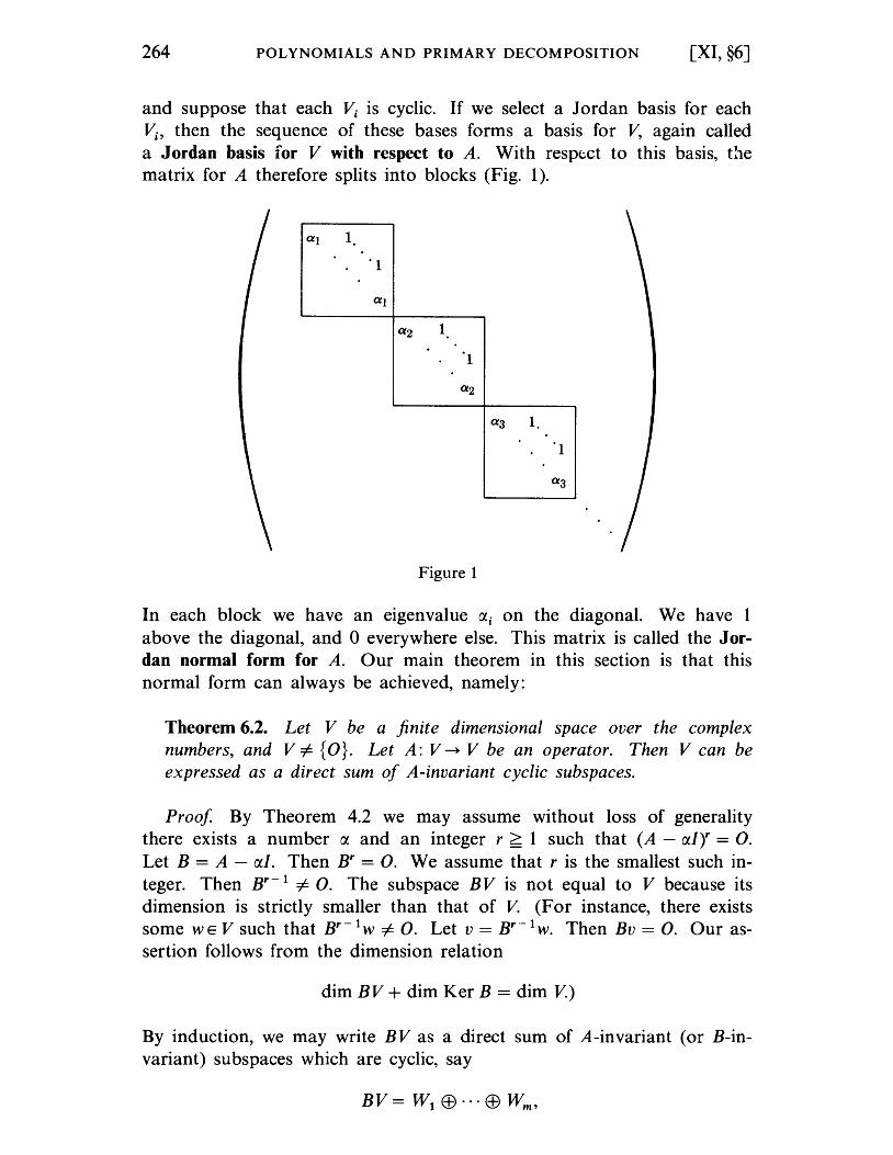
264 POLYNOMIALS AND PRIMARY DECOMPOSITION [XI, §6]
and suppose that each Vi is cyclic. If we select a Jordan basis for each Vi' then the sequence of these bases forms a basis for V, again called a Jordan basis for V with respect to A. With resp(;'ct to this basis, t!le matrix for A therefore splits into blocks (Fig. 1).
al 1
·1
al
a2 1
1
a2
a3 1.
·1
a3
Figure 1
In each block we have an eigenvalue rx i on the diagonal. We have 1 above the diagonal, and 0 everywhere else. This matrix is called the Jordan normal form for A. Our main theorem in this section is that this normal form can always be achieved, namely:
Theorem 6.2. Let V be a finite dimensional space over the complex numbers, and V i= {O}. Let A: V --+ V be an operator. Then V can be expressed as a direct sum of A-invariant cyclic subspaces.
Proof By Theorem 4.2 we may assume without loss of generality there exists a number rx and an integer r > 1 such that (A - rxIr = O. Let B = A - rxI. Then Br = o. We assume that r is the smallest such integer. Then Br-l i= O. The subspace BV is not equal to V because its dimension is strictly smaller than that of V. (For instance, there exists some WE V such that Br-lw i= O. Let v = Br-l w. Then Bv = O. Our assertion follows from the dimension relation
dim BV + dim Ker B = dim V.)
By induction, we may write BV as a direct sum of A-invariant (or B-invariant) subspaces which are cyclic, say
[XI, §6] THE JORDAN NORMAL FORM 265
such that Wi has a basis consisting of elements Bkw i for some cyclic vector WiE Wi of period rio Let ViE V be such that BVi = Wi. Then each Vi is a cyclic vector, because
Let ~ be the subspace of V generated by the elements Bkvi for k = 0, ... ,rio We contend that the subspace V' equal to the sum
V' = V + ... + V I m
is a direct sum. We have to prove that any element u in this sum can be expressed uniquely in the form
Any element of ~ is of type h(B)Vi where h is a polynomial, of degree < rio Suppose that
(1)
Applying B and noting that Bfi(B) = fi(B)B we get
But WI + ... + Wm is a direct sum decomposition of BV, whence
all i = 1, ... ,me
Therefore tri divides flt), and in particular t divides flt). We can thus write
for some polynomial gi' and hence fi(B) = gi(B)B. It follows from (1) that
Again, tri divides gi(t), whence tri + I divides fi(t), and therefore fi(B)Vi = o. This proves what we wanted, namely that V'is a direct sum of VI' ... ' Vm •
From the construction of V' we observe that BV' = BV, because any element in BV is of the form
266 POLYNOMIALS AND PRIMARY DECOMPOSITION [XI, §6]
with some polynomials ii' and is therefore the image under B of the element
which lies in V'. From this we shall conclude that
V= V' + Ker B.
Indeed, let v E V. Then Bv = Bv' for some v' E V', and hence B(v - v') = O. Thus
v = v' + (v - v'),
thus proving that V = V' + Ker B. Of course this sum is not direct. However, let [J4' be a Jordan basis of V'. We can extend [J4' to a basis of V by using elements of Ker B. Namely, if {u 1, ••. ,us} is a basis of Ker B, then
is a basis of V for suitable indices j 1' ... ,j,. Each uj satisfies BUj = 0, whence uj is an eigenvector for A, and the one-dimensional space generated by U j is A -invariant, and cyclic. We let this subspace be denoted by U j • Then we have
V = V' ffi U· ffi ... ffi U· Jl Jl
thus gIvIng the desired expression of V as a direct sum of cyclic subspaces. This proves our theorem.
XI, §6. EXERCISES
In the following exercises, we let V be a finite dimensional vector space over the complex numbers, and we let A: V --+- V be an operator.
1. Show that A can be written in the form A = D + N, where D is a diagonalizable operator, N is a nilpotent operator, and DN = ND.
2. Assume that V is cyclic. Show that the subspace of V generated by eigenvectors of A is one-dimensional.
[XI, §6] THE JORDAN NORMAL FORM 267
3. Assume that V is cyclic. Let f be a polynomial. What are the eigenvalues of f(A) in terms of those of A? Same question when V is not assumed cyclic.
4. If A is nilpotent and not 0, show that A is not diagonalizable.
5. Let P A be the characteristic polynomial of A, and write it as a product
r
P A(t) = n (t - Cti)m i,
i= 1
where Ct i, ••• ,Ctr are distinct. Let f be a polynomial. Express the characteristic polynomial P f(A) as a product of factors of degree 1.
A direct sum decomposition of matrices
6. Let Matn (C) be the vector space of n x n complex matrices. Let Eij for i, j == 1, ... ,n be the matrix with (ij)-component 1, and all other components O. Then the set of elements Eij is a basis for Matn(C). Let D* be the set of diagonal matrices with non-zero diagonal components. We write such a matrix as diag(at, ... , an) == a. We define the conjugation action of D* on Matn(C) by
c(a)X == aXa- I.
(a) Show that a 1---+ c(a) is a map from D* into the automorphisrris of Matn(C) (isomorphisms of Matn (C) with itself), satisfying
c(/) == id, c(ab) == c(a)c(b) and
A map satisfying these conditions is called a bomomorphism. (b) Show that each Eij is an eigenvector for the action of c(a), the eigenvalue
being given by Xij(a) == ai/aj. Thus Matn(C) is a direct sum o'f eigenspaces. Each Xij: D* -+ C* is a homomorphism of D* into the multiplicative group of complex numbers.
7. For two matrices X, Y E Matn(C), define [X, Y] == XY - YX. Let Lx denote the map such that Lx( Y) == [X, Y]. One calls Lx the bracket (or regular or Lie) action of X. (a) Show that for each X, the map Lx: Y 1---+ [X, Y] is a linear map, satisfying
the Leibniz rule for derivations, that is [X, [Y, Z]] == [[X, Y], Z] + [Y, [X, Z]]. (b) Let D be the vector space of diagonal matrices. For each HE D, show that
Eij is an eigenvector of L H , with eigenvalue Ctij(H) == hi - hj (if hI, ... ,hn are the diagonal components of H). Show that Ctij: D -+ C is linear. It is called an eigencbaracter of the bracket action.
(c) For two linear maps A, B of a vector space V into itself, define
[A, B] == AB - BA. Show that L[x, Y] == [Lx, Ly].
CHAPTER XII
Convex Sets
XII, §1. DEFINITIONS
Let S be a subset of Rm. We say that S is convex if given points P, Q in S, the line segment joining P to Q is also oontained in S.
We recall that the line segment joining P to Q is the set of all points P + t(Q - P) with 0 < t < 1. Thus it is the set of points
(1 - t)P + tQ, with 0 < t < 1.
Theorem 1.1. Let P l' ... ,P n be points of Rm. The set of all linear combinations
with 0 < Xi < 1 and Xl + ... + Xn = 1, is a convex set.
Theorem 1.2. Let P l' ... ,P n be points of Rm. Any convex set which contains P l' ... ,P n also contains all linear combinations
such that 0 < Xi < 1 for all i, and Xl + ... + X" -= 1.
Either work out the proofs as art exercise or look them up in Chapter III, §5.
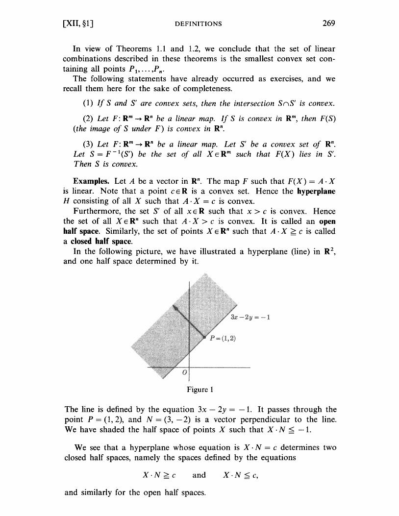
[XII, §1] DEFINITIONS 269
In view of Theorems 1.1 and 1.2, we conclude that the set of linear combinations described in these theorems is the smallest convex set containing all points P l' ... ,P n •
The following statements have already occurred as exercises, and we recall them here for the sake of completeness.
(1) If Sand S' are convex sets, then the intersection S nS' is convex.
(2) Let F: Rm --+ Rn be a linear map. If S is convex in Rm, then F(S) (the image of S under F) is convex in Rn.
(3) Let F: Rm --+ Rn be a linear map. Let S' be a convex set of Rn. Let S = F -1(S') be the set of all X E Rm such that F(X) lies in S'. Then S is convex.
Examples. Let A be a vector in Rn. The map F such that F(X) = A· X is linear. Note that a point c E R is a convex set. Hence the hyperplane H consisting of all X such that A· X = c is convex.
Furthermore, the set S' of all x E R such that x > c is convex. Hence the set of all X E Rn such that A· X > c is convex. It is called an open half space. Similarly, the set of points X E Rn such that A· X > c is called a closed half space.
In the following picture, we have illustrated a hyperplane (line) in R2, and one half space determined by it.
Figure 1
The line is defined by the equation 3x - 2y = -1. It passes through the point P = (1, 2), and N = (3, - 2) is a vector perpendicular to the line. We have shaded the half space of points X such that X· N < -1.
We see that a hyperplane whose equation is X· N = c determines two closed half spaces, namely the spaces defined by the equations
X·N>c and X·N < c,
and similarly for the open half spaces.
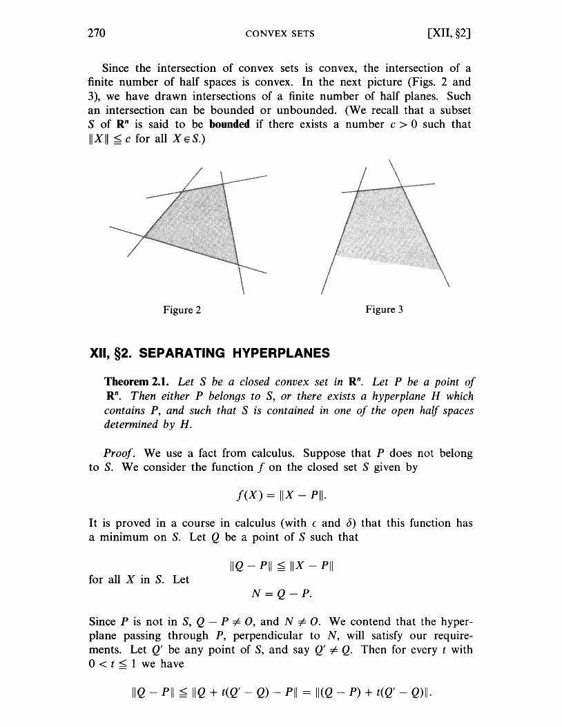
270 CONVEX SETS [XII, §2]
Since the intersection of convex sets is convex, the intersection of a finite number of half spaces is convex. In the next picture (Figs. 2 and 3), we have drawn intersections of a finite number of half planes. Such an intersection can be bounded or unbounded. (We recall that a subset S of Rn is said to be bounded if there exists a number c > 0 such that IIXII < c for all XES.)
Figure 2 Figure 3
XII, §2. SEPARATING HYPERPLANES
Theorem 2.1. Let S be a closed convex set in Rn. Let P be a point of Rn. Then either P belongs to S, or there exists a hyperplane H which contains P, and such that S is contained in one of the open half spaces determined by H.
Proof. We use a fact from calculus. Suppose that P does not belong to S. We consider the function f on the closed set S given by
f(X) = IIX - PII·
It is proved in a course in calculus (with ( and b) that this function has a minimum on S. Let Q be a point of S such that
IIQ - PII < IIX - PII for all X in S. Let
N = Q - P.
Since P is not in S, Q - P =1= 0, and N =1= o. We contend that the hyperplane passing through P, perpendicular to N, will satisfy our requirements. Let Q' be any point of S, and say Q' =1= Q. Then for every t with o < t < 1 we have
IIQ - PII < IIQ + t(Q' - Q) - PII = II(Q - P) + t(Q' - Q)II·
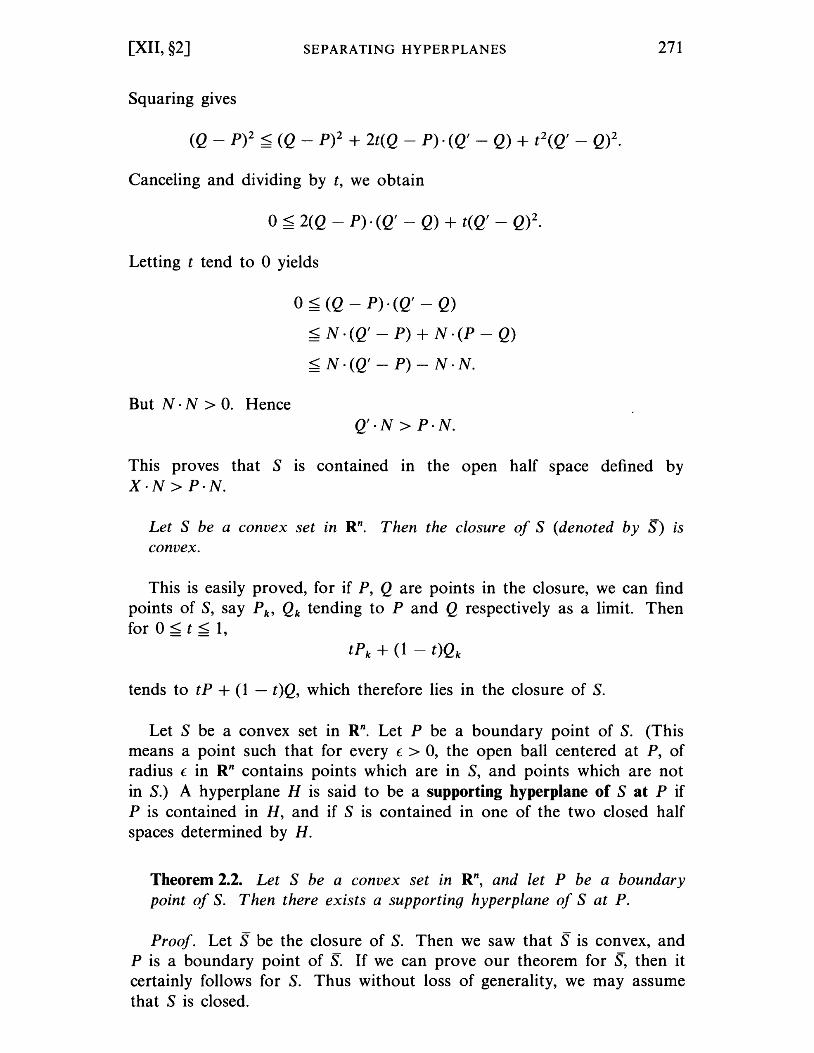
[XII, §2] SEPARATING HYPERPLANES
Squaring gives
(Q _ p)2 < (Q _ p)2 + 2t(Q _ P). (Q' _ Q) + t2(Q' _ Q)2.
Canceling and dividing by t, we obtain
o <2(Q - P)·(Q' - Q) + t(Q' - Q)2.
Letting t tend to 0 yields
But N· N > O. Hence
o < (Q - P)· (Q' - Q)
< N .(Q' - P) + N ·(P - Q)
< N·(Q' - P) - N·N.
Q'·N > P·N.
271
This proves that S IS contained in the open half space defined by X·N>P·N.
Let S be a convex set in Rn. Then the closure of S (denoted by S) is convex.
This is easily proved, for if P, Q are points in the closure, we can find points of S, say P k' Qk tending to P and Q respectively as a limit. Then for 0 < t < 1,
tends to tP + (1 - t)Q, which therefore lies in the closure of S.
Let S be a convex set in Rn. Let P be a boundary point of S. (This means a point such that for every l > 0, the open ball centered at P, of radius l in Rn contains points which are in S, and points which are not in S.) A hyperplane H is said to be a supporting hyperplane of S at P if P is contained in H, and if S is contained in one of the two closed half spaces determined by H.
Theorem 2.2. Let S be a convex set in Rn, and let P be a boundary
point of S. Then there exists a supporting hyperplane of S at P.
Proof. Let S be the closure of S. Then we saw that S is convex, and P is a boundary point of S. If we can prove our theorem for S, then it certainly follows for S. Thus without loss of generality, we may assume that S is closed.
272 CONVEX SETS [XII, §3]
For each integer k > 2, we can find a point P k not in S, but at distance < 11k from P. By Theorem 2.1, we find a point Qk on S whose distance from Pk is minimal, and we let Nk = Qk - Pk. Let N~ be the vector in the same direction as N k but of norm 1. The sequence of vectors N'k has a point of accumulation on the sphere of radius 1, say N', because the sphere is compact. We have by Theorem 2.1, for all XES,
for every k, whence dividing each side by the norm of N k , we get
for every k. Since N' is a point of accumulation of {N~}, and since P is a limit of {P k}, it follows by continuity that for each X in S,
X·N'>P·N'. This proves our theorem.
Remark. Let S be a convex set, and let H be a hyperplane defined by an equation
X·N=a.
Assume that for all XES we have X· N > a. If P is a point of S lying in the hyperplane, then P is a boundary point of S. Otherwise, for i > 0 and i sufficiently small, P - iN would be a point of S, and thus
(P - iN) . N = p. N - iN . N = a - iN . N < a,
contrary to hypothesis. We conclude therefore that H is a supporting hyperplane of S at P.
XII, §3. EXTREME POINTS AND SUPPORTING HYPERPLANES
Let S be a convex set and let P be a point of S. We shall say that P is an extreme point of S if there do not exist points Ql' Q2 of S with Ql #- Q2 such that P can be written in the form
P = tQl + (1 - t)Q2 with 0 < t < 1.
In other words, P cannot lie on a line segment contained in S unless it is one of the end-points of the line segment.
[XII, §3] EXTREME POINTS AND SUPPORTING HYPERPLANES 273
Theorem 3.1. Let S be a closed convex set which is bounded. Then every supporting hyperplane of S contains an extreme point.
Proof. Let H be a supporting hyperplane, defined by the equation X . N = Po . N at a boundary point Po, and say X· N > Po . N for all XES. Let T be the intersection of S and the hyperplane. Then T is convex, closed, bounded. We contend that an extreme point of Twill also be an extreme point of S. This will reduce our problem to finding extreme points of T To prove our contention let P be an extreme point of T, and suppose that we can write
o < t < 1.
Dotting with N, and using the fact that P is in the hyperplane, hence p. N = po· N, we obtain
(1)
We have Ql·N and Q2·N > Po·N since Ql' Q2 lie in S. If one of these IS > Po·N, say Ql·N > Po·N, then the right-hand side of equation (1) IS
and this is impossible. Hence both Ql' Q2 lie in the hyperplane, thereby contradicting the hypothesis that P is an extreme point of T.
We shall now find an extreme point of T. Among all points of T, there is at least one point whose first coordinate is smallest, because T is closed and bounded. (We project on the first coordinate. The image of T under this projection has a greatest lower bound which is taken on by an element of T since T is closed.) Let Tl be the subset of T consisting of all points whose first coordinate is equal to this smallest one. Then Tl is closed, and bounded. Hence we can find a point of Tl whose second coordinate is smallest among all points of T1 ,
and the set T2 of all points of Tl having this second coordinate is closed and bounded. We may proceed in this way until we find a point P of T having successively smallest first, second, ... ,n-th coordinate. We assert that P is an extreme point of T. Let
P = (PI'··· ,Pn)· Suppose that we can write
P = tX + (1 - t)Y, o < t < 1,
274 CONVEX SETS [XII, §4]
and points X = (Xl' ... ,xn), Y = (Yl, ... ,Yn) In T. Then Xl and Yl > Pl'
and
If Xl or Yl > Pl' then
which is impossible. Hence Xl = Yl = Pl. Proceeding inductively, suppose we have proved Xi = Yi = Pi for i = 1, ... ,r. Then if r < n,
Pr+ 1 = txr+ 1 + (1 - t)Yr+ l'
and we may repeat the preceding argument. It follows that
X = Y = P,
whence P is an extreme point, and our theorem is proved.
XII, §4. THE KREIN-MILMAN THEOREM
Let E be a set of points in Rn (with at least one point in it). We wish to describe the smallest convex set containing E. We may say that it is the intersection of all convex sets containing E, because this intersection is convex, and is clearly smallest.
We can also describe this smallest convex set in another way. Let EC
be the set of all linear combinations
of points P 1' ... ,Pm in E with real coefficients ti such that
and
Then the set EC is convex. We leave the trivial verification to the reader. Any convex set containing E must contain E C
, and hence E C is the smallest convex set containing E. We call E C the convex closure of E.
Let S be a convex set and let E be the set of its extreme points. Then EC is contained in S. We ask for conditions under which EC = S.
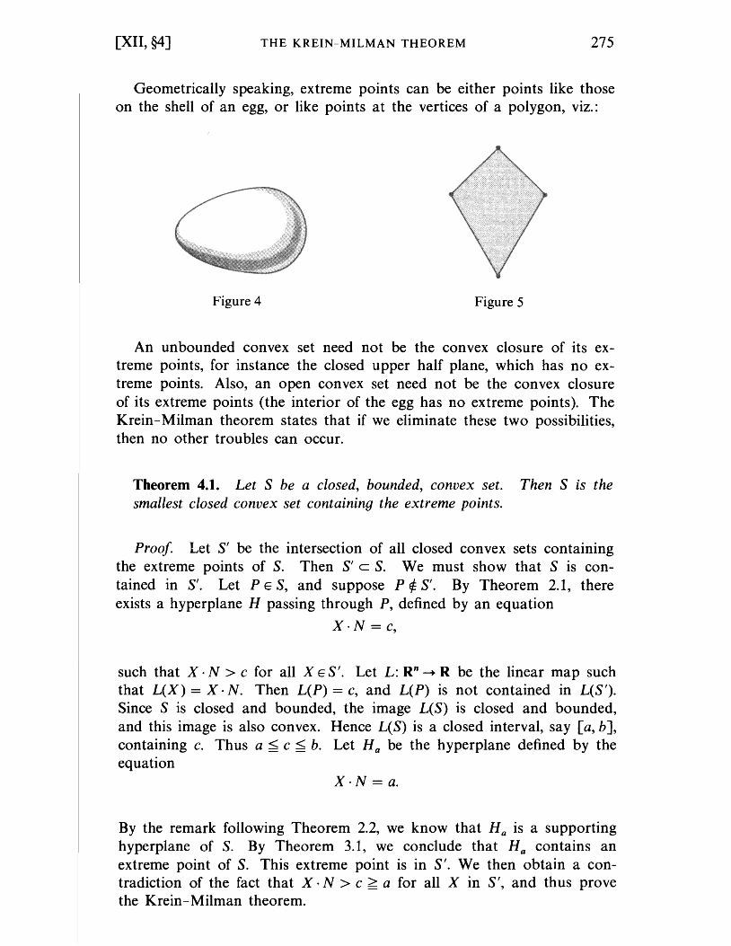
[XII, §4] THE KREIN-MILMAN THEOREM 275
Geometrically speaking, extreme points can be either points like those on the shell of an egg, or like points at the vertices of a polygon, viz.:
Figure 4 Figure 5
An unbounded convex set need not be the convex closure of its extreme points, for instance the closed upper half plane, which has no extreme points. Also, an open convex set need not be the convex closure of its extreme points (the interior of the egg has no extreme points). The Krein-Milman theorem states that if we eliminate these two possibilities, then no other troubles can occur.
Theorem 4.1. Let S be a closed, bounded, convex set. Then S is the smallest closed convex set containing the extreme points.
Proof. Let S' be the intersection of all closed convex sets containing the extreme points of S. Then S' c S. We must show that S is contained in S'. Let PES, and suppose P ~ S'. By Theorem 2.1, there exists a hyperplane H passing through P, defined by an equation
X·N = c,
such that X· N > c for all XES'. Let L: Rn ~ R be the linear map such that L(X) = X . N. Then L(P) = c, and L(P) is not contained in L(S'). Since S is closed and bounded, the image L(S) is closed and bounded, and this image is also convex. Hence L(S) is a closed interval, say [a, b], containing c. Thus a < c < b. Let Ha be the hyperplane defined by the equation
X·N=a.
By the remark following Theorem 2.2, we know that Ha is a supporting hyperplane of S. By Theorem 3.1, we conclude that Ha contains an extreme point of S. This extreme point is in S'. We then obtain a contradiction of the fact that X· N > c > a for all X in S', and thus prove the Krein-Milman theorem.
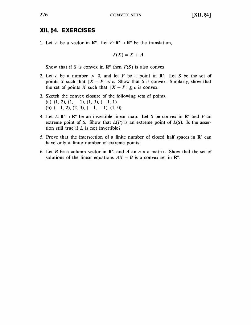
276 CONVEX SETS [XII, §4]
XII, §4. EXERCISES
1. Let A be a vector in Rn. Let F: Rn -+ Rn be the translation,
F(X) = X + A.
Show that if S is convex in Rn then F(S) is also convex.
2. Let c be a number > 0, and let P be a point in Rn. Let S be the set of points X such that IIX - PII < c. Show that S is convex. Similarly, show that the set of points X such that II X - P II ~ c is convex.
3. Sketch the convex closure of the following sets of points. ( a) ( 1, 2), (1, - 1), (1, 3), ( - 1, 1) (b) (-1, 2), (2, 3), (-1, -1), (1, 0)
4. Let L: Rn -+ Rn be an invertible linear map. Let S be convex in Rn and P an extreme point of S. Show that L(P) is an extreme point of L(S). Is the assertion still true if L is not invertible?
5. Prove that the intersection of a finite number of closed half spaces in Rn can have only a finite number of extreme points.
6. Let B be a column vector in Rn, and A an n x n matrix. Show that the set of
solutions of the linear equations AX = B is a convex set in Rn.
APPENDIX
Complex Numbers
The complex numbers are a set of objects which can be added and multiplied, the sum and product of two complex numbers being also a complex number, and satisfy the following conditions.
(1) Every real number is a complex number, and if ~, P are real numbers, then their sum and product as complex numbers are the same as their sum and product as real numbers.
(2) There is a complex number denoted by i such that i2 = -1.
(3) Every complex number can be written uniquely in the form a + bi where a, b are real numbers.
(4) The ordinary laws of arithmetic concerning addition and multiplication are satisfied. We list these laws:
If ~, p, yare complex numbers, then
(~P)y = ~(Py) and (~ + p) + y = ~ + (p + y).
We have ~(p + y) = ~p + ~y, and (P + y)~ = p~ + y~. We ha ve ~p = p~, and ~ + p = p + ~. If 1 is the real number one, then 1~ = ~. If 0 is the real number zero, then o~ = o. We have ~+(-l)~=O.
We shall now draw consequences of these properties. With each complex number a + bi, we associate the vector (a, b) in the plane. Let ~ = a l + a2 i and p = b i + b2 i be two complex numbers. Then
~ + P = a l + hI + (a 2 + b2 )i.
278 COMPLEX NUMBERS [APP. I]
Hence addition of complex numbers is carried out "componentwise" and corresponds to addition of vectors in the plane. F or example,
(2 + 3i) + ( - 1 + 5i) = 1 + 8i.
In multiplying complex numbers, we use the rule i2 = -1 to simplify a product and to put it in the form a + bi. For instance, let rx = 2 + 3i and f3 = 1 - i. Then
rxf3 = (2 + 3i)(1 - i) = 2(1 - i) + 3i(1 - i)
= 2 - 2i + 3i - 3i2
= 2 + i - 3( -1)
=2+3+i
=5+i.
Let rx = a + bi be a complex number. We define ~ to be a - bi. Thus if rx = 2 + 3i, then ~ = 2 - 3i. The complex number ~ is called the conjugate of rx. We see at once that
With the vector interpretation of complex numbers, we see that rx~ is the square of the distance of the point (a, b) from the origin.
We now have one more important property of complex numbers, which will allow us to divide by complex numbers other than 0.
If rx = a + bi is a complex number #- 0, and if we let
then rxA = Arx = 1. The proof of this property is an immediate consequence of the law of
multiplication of complex numbers, because
The number A above is called the inverse of rx, and is denoted by rx- 1 or l/rx. If rx, f3 are complex numbers, we often write f3lrx instead of rx - 1 f3 (or f3rx- 1
), just as we did with real numbers. We see that we can divide by complex numbers #- 0.
[APP. I] COMPLEX NUMBERS 279
We define the absolute value of a complex number rx = a1 + ia2 to be
Irxl = Jai + a~.
This absolute value is none other than the norm of the vector (a 1 , a2 ).
In terms of absolute values, we can write
provided rx =1= o. The triangle inequality for the norm of vectors can now be stated for
complex numbers. If rx, P are complex numbers, then
Irx + PI < Irxl + IPI.
Another property of the absolute value is given in Exercise 5. Using some elementary facts of analysis, we shall now prove:
Theorem. The complex numbers are algebraically closed, in other words, every polynomial f E C[t] of degree > 1 has a root in C.
Proof We may write
I( ) n n-1 t = an t + an - 1 t + ... + ao
with an #- O. For every real R > 0, the function I I I such that
t ~ If(t)1
is continuous on the closed disc of radius R, and hence has a minimum value on this disc. On the other hand, from the expression
we see that when I t I becomes large, then II (t) I also becomes large, i.e. given C > 0 there exists R > 0 such that if It I > R then I/(t)1 > C. Consequently, there exists a positive number Ro such that, if Zo is a minimum point of Ilion the closed disc of radius Ro, then
I/(t)1 > I/(zo)1
for all complex numbers t. In other words, Zo is an absolute minimum for III. We shall prove that I(zo) = O.
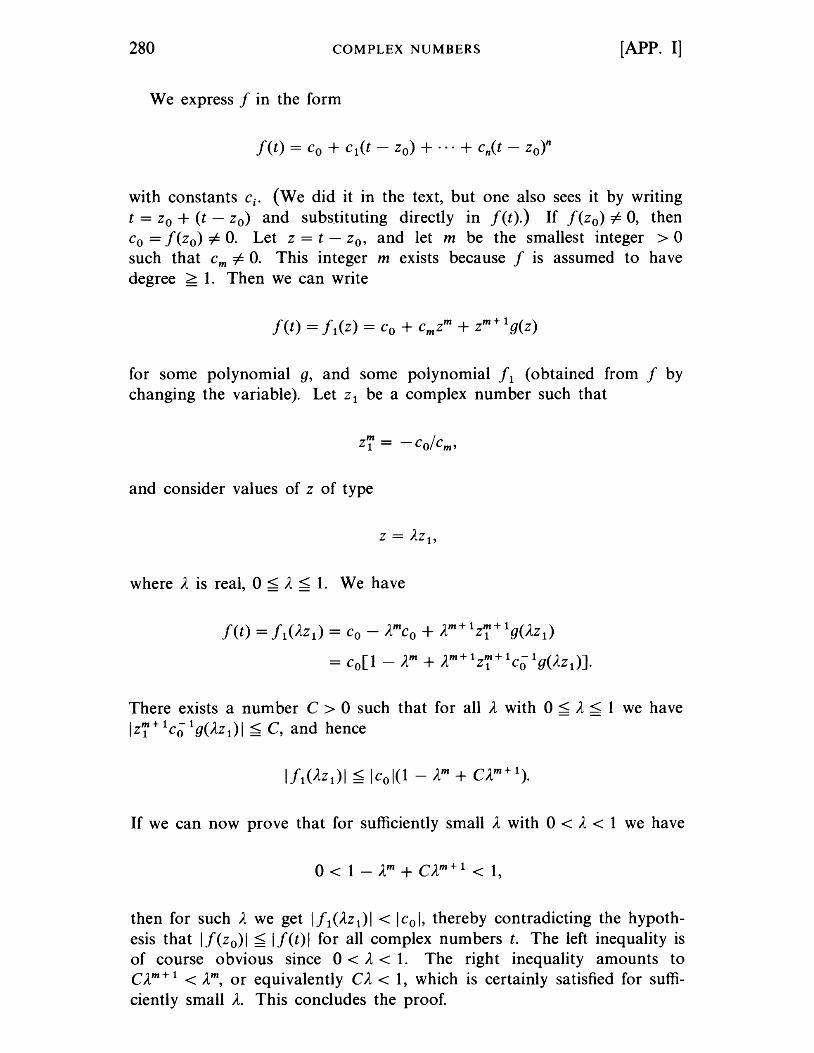
280 COMPLEX NUMBERS [APP. I]
We express f in the form
with constants Ci • (We did it in the text, but one also sees it by writing t = Zo + (t - zo) and subs.tituting directly in f(t).) If f(zo);/= 0, then Co = f(zo) ;/= O. Let z = t - zo, and let m be the smallest integer > 0 such that cm ;/= O. This integer m exists because f is assumed to have degree > 1. Then we can write
for some polynomial g, and some polynomial fl (obtained from f by changing the variable). Let Zl be a complex number such that
and consider values of z of type
where A is real, 0 < A <1. We have
f(t) = fl(AZ l ) = Co - AmCo + Am+ lz7+ 19(AZl )
= co[1 - Am + Am+ lz7+ lCO 19(AZl )].
There exists a number C > 0 such that for all A with 0 < A s 1 we have Iz7+ lCO 19(AZl)1 < C, and hence
If we can now prove that for sufficiently small A with 0 < A < 1 we have
then for such A we get Ifl(AZl)1 < Icol, thereby contradicting the hypothesis that I f(zo)1 < I f(t)1 for all complex numbers t. The left inequality is of course obvious since 0 < A < 1. The right inequality amounts to CAm+ 1 < Am, or equivalently CA < 1, which is certainly satisfied for sufficiently small A. This concludes the proof.
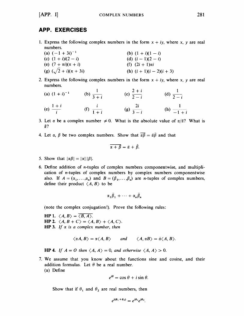
[APP. I] COMPLEX NUMBERS 281
APP. EXERCISES
1. Express the following complex numbers in the form x + iy, where x, yare real numbers. (a) (-1 + 3i) - 1
(c) (1 + i)i(2 - i) (e) (7 + ni)(n + i)
(b) (1 + i)( 1 - i) ( d) (i - 1)(2 - i)
(f) (2i + 1 )ni
(g) (J2 + i)(n + 3i) (h) (i + 1)(i - 2)(i + 3)
2. Express the following complex numbers in the form x + iy, where x, yare real numbers.
(a) (1 + 0- 1
1 + i (e) -.
I
1 (b) 3 + i
i (f) 1 + i
2+i (c) -.
2 - I
2i (g) 3 - i
1 (d) -.
2 - I
1 (h) -1 + i
3. Let tY. be a complex number =I- o. What is the absolute value of tY./a? What is =? tY..
4. Let tY., f3 be two complex numbers. Show that tY.f3 = ap and that
5. Show that 1tY.f31 = 1tY.11f31.
6. Define addition of n-tuples of complex numbers componentwise, and multiplication of n-tuples of complex numbers by complex numbers componentwise also. If A = (tY. 1, ... ,tY.n) and B = (f31' ... ,f3n) are n-tuples of complex numbers, define their product (A, B) to be
(note the complex conjugation!). Prove the following rules:
UP 1. (A, B) = (B, A). UP 2. (A, B + C) = (A, B) + (A, C). UP 3. If tY. is a complex number, then
(tY.A, B) = tY.(A, B) and (A, tY.B) = a(A, B).
UP 4. If A = 0 then (A, A) = 0, and otherwise (A, A) > O.
7. We assume that you know about the functions sine and cosine, and their addition formulas. Let f) be a real number. (a) Define
ei8 = cos f) + i sin f).
Show that if (}1 and f)2 are real numbers, then
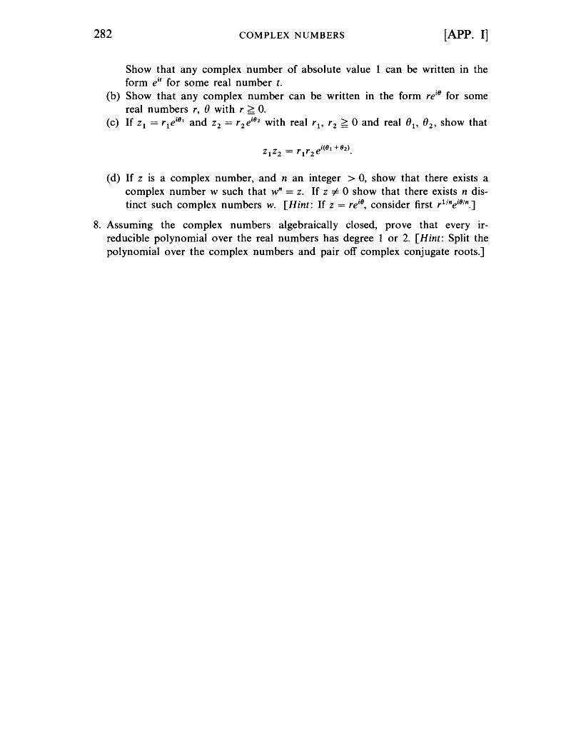
282 COMPLEX NUMBERS [APP. I]
Show that any complex number of absolute value 1 can be written in the form eit for some real number t.
(b) Show that any complex number can be written in the form rei8 for some
real numbers r, f) with r ~ o. (c) If ZI = r 1e
i81 and Z2 = r 2 ei82 with real r l , r 2 ~ 0 and real f)1' f)2' show that
(d) If Z is a complex number, and n an integer > 0, show that there exists a complex number w such that wn = z. If z =I- 0 show that there exists n distinct such complex numbers w. [Hint: If z = re
i8, consider first rl/ne
i8/n.]
8. Assuming the complex numbers algebraically closed, prove that every irreducible polynomial over the real numbers has degree 1 or 2. [Hint: Split the polynomial over the complex numbers and pair off complex conjugate roots.]
APPENDIX II
Iwasawa Decomposition and Others
Let SLn denote the set of matrices with determinant 1. The purpose of this appendix is to formulate in some general terms results about SLn. We shall use the language of group theory, which has not been used previously, so we have to start with the definition of a group.
Let G be a set. We are given a mapping G x G ~ G, which at first we write as a product, i.e. to each pair of elements (x, y) of G we associate an element of G denoted by xy, satisfying the following axioms.
GR 1. The product is associative, namely for all x, y, Z E G we have
(xY)Z = x(yz).
GR 2. There is an element e E G such that ex = xe = x for all x E G.
GR 3. Given x E G there exists an element x-I E G such that
It is an easy exercise to show that the element in GR 2 is uniquely determined, and it is called the unit element. The element x-I in GR 3 is also easily shown to be uniquely determined, and is called the inverse of x. A set together with a mapping satisfying the three axioms is called a group.
Example. Let G' = SLn(R). Let the product be the mUltiplication of matrices. Then SLn(R) is a group. Similarly, SLn(C) is a group. The unit element is the unit matrix I.
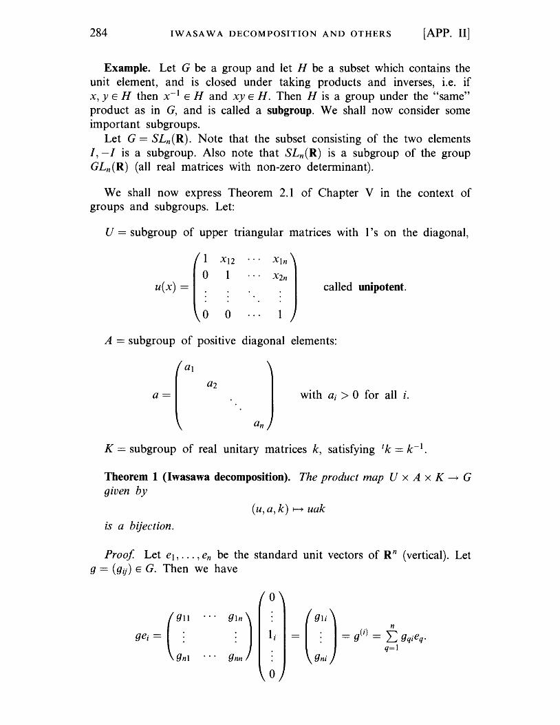
284 IW ASA W A DECOMPOSITION AND OTHERS [APP. II]
Example. Let G be a group and let H be a subset which contains the unit element, and is closed under taking products and inverses, i.e. if x, y E H then x-I E Hand xy E H. Then H is a group under the "same" product as in G, and is called a subgroup. We shall now consider some important subgroups.
Let G = SLn(R). Note that the subset consisting of the two elements I, -I is a subgroup. Also note that SLn(R) is a subgroup of the group GLn{R) (all real matrices with non-zero determinant).
We shall now express Theorem 2.1 of Chapter V In the context of groups and subgroups. Let:
U = subgroup of upper triangular matrices with 1 's on the diagonal,
1 XI2 XIn
o 1 X2n
u(X) = called unipotent.
001
A = subgroup of positive diagonal elements:
a= with ai > 0 for all i.
K = subgroup of real unitary matrices k, satisfying tk = k- l .
Theorem 1 (Iwasawa decomposition). The product map U x A x K ----t G given by
(u, a, k) 1---+ uak
is a bijection.
Proof Let eI, . .. ,en be the standard unit vectors of R n (vertical). Let g = (gij) E G. Then we have
o
o
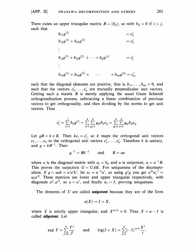
[APP. II] IW ASA W A DECOMPOSITION AND OTHERS 285
There exists an upper triangular matrix B == (bij), so with bij == 0 if i > j, such that
b ll gO)
b 12g(1) + b22g(2)
== e~ }
such that the diagonal elements are positive, that is b11 , ... , bnn > 0, and such that the vectors ei, ... , e~ are mutually perpendicular unit vectors. Getting such a matrix B is merely applying the usual Gram Schmidt orthogonalization process, subtracting a linear combination of previous vectors to get orthogonality, and then dividing by the norms to get unit vectors. Thus
) n n n n e; == L bijg(i) == L L gq;bijeq == L L gq;bijeq.
;=1 ;=1 q=1 q=1 ;=1
Let gB == k E K. Then ke; == e;, so k maps the orthogonal unit vectors e1, ... ,en to the orthogonal unit vectors ei, .. . ,e~. Therefore k is unitary, and g == kB- 1• Then
g-l == Bk-1 and B == au
where a is the diagonal matrix with a; == bu and u is unipotent, u == a-I B.
This proves the surjection G == UAK. For uniqueness of the decomposition, if g == uak == u' a' k', let U1 == u-1 u', so using gt g you get a 2tu11 == U1a,2. These matrices are lower and upper triangular respectively, with diagonals a2, a,2, so a == a', and finally U1 == /, proving uniqueness.
The elements of U are called unipotent because they are of the form
u(X) == / + X,
where X is strictly upper triangular, and xn+1 == O. Thus X == u - / IS
called nilpotent. Let
00 y) exp Y == 2:-.,
)=0 J. and
00 X; log(/ +X) == 2:(_I)Z+I_ ..
;=1 1
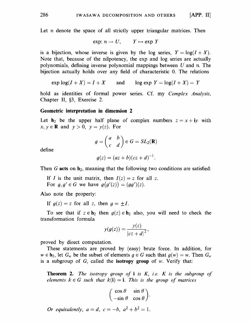
286 IW ASA W A DECOMPOSITION AND OTHERS [APP. II]
Let n denote the space of all strictly upper triangular matrices. Then
exp: n ----t U, y 1---+ exp Y
is a bijection, whose inverse is given by the log series, Y == log( I + X). Note that, because of the nilpotency, the exp and log series are actually polynomials, defining inverse polynomial mappings between U and n. The bijection actually holds over any field of characteristic O. The relations
exp 10g(1 + X) == I + X and log exp Y == 10g(1 + X) == Y
hold as identities of formal power series. Cf. my Complex Analysis, Chapter II, §3, Exercise 2.
Geometric interpretation in dimension 2
Let h2 be the upper half plane of complex numbers z == x + iy with x, y E Rand y > 0, y == y(z). For
define
g = (: !) E G = SL2(R)
g(z) == (az + b)(cz + d)-I.
Then G acts on h2, meaning that the following two conditions are satisfied:
If I is the unit matrix, then I(z) == z for all z. For g,g' E G we have g(g'(z)) == (gg')(z).
Also note the property:
If g(z) == z for all z, then g == + I. To see that if z E h2 then g(z) E h2 also, you will need to check the
transformation formula y(z)
y(g(z)) = Icz + d1 2 '
proved by direct computation. These statements are proved by (easy) brute force. In addition, for
w E h2, let Gw be the subset of elements g E G such that g(w) == w. Then Gw
is a subgroup of G, called the isotropy group of w. Verify that:
Theorem 2. The isotropy group of i is K, i. e. K is the subgroup of elements kEG such that k(i) == i. This is the group of matrices
(
COS () sin () ) -sin () cos () .
Or equivalently, a == d, c == -b, a2 + b2 == 1.
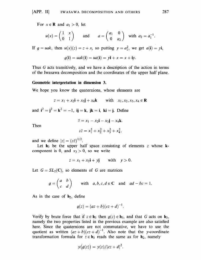
[APP. II] IW ASA W A DECOMPOSITION AND OTHERS 287
For x E Rand al > 0, let
u(x) = (~ ~) a=(~ ° ) . h 1 WIt a2 == al . a2
and
If 9 == uak, then u(x)(z) == z + x, so putting y == al, we get a(i) == yi,
g(i) == uak(i) == ua(i) == yi + x == x + iy.
Thus G acts transitively, and we have a description of the action in terms of the Iwasawa decomposition and the coordinates of the upper half plane.
Geometric interpretation in dimension 3.
We hope you know the quaternions, whose elements are
and i2 == j2 == k 2 == -1, ij == k, jk == i, ki == j. Define
Then - 2 2 2 2
ZZ==XI +X2 +X3 +X4'
and we define Izi == (zz) 1/2.
Let h3 be the upper half space consIstIng of elements z whose kcomponent is 0, and X3 > 0, so we write
with y > 0.
Let G == SL2(C), so elements of G are matrices
with a, b, e, dEC and ad - be == 1.
As in the case of h2, define
9 ( z) == (az + b) (ez + d) -1 .
Verify by brute force that if z E h3 then g(z) E h3, and that G acts on h3, namely the two properties listed in the previous example are also satisfied here. Since the quaternions are not commutative, we have to use the quotient as written (az + b)(ez + d)-I. Also note that the y-coordinate transformation formula for z E h3 reads the same as for h2, namely
y(g(z)) == y(z)/lez + d1 2.
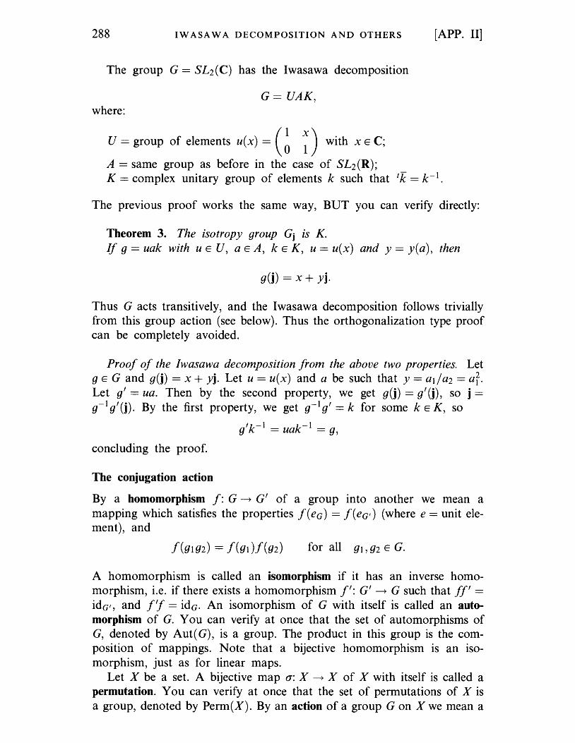
288 IW ASA W A DECOMPOSITION AND OTHERS
The group G = SL2(C) has the Iwasawa decomposition
G= UAK, where:
U = group of elements u(x) = (~ ~) with x E C;
A = same group as before in the case of SL2(R);
[APP. II]
K = complex unitary group of elements k such that ll( = k- l •
The previous proof works the same way, BUT you can verify directly:
Theorem 3. The isotropy group Gj is K. If g = uak with u E U, a E A, k E K, u = u(x) and y = y(a), then
gO) = x + yj.
Thus G acts transitively, and the Iwasawa decomposition follows trivially from this group action (see below). Thus the orthogonalization type proof can be completely avoided.
Prool 01 the Iwasawa decomposition Irom the above two properties. Let g E G and g(j) = x + yj. Let u = u(x) and a be such that y = al/a2 = a? Let g' = ua. Then by the second property, we get gO) = g'(j), so j = g-l g' 0). By the first property, we get g-l g' = k for some k E K, so
g'k- l = uak- l = g,
concluding the proof.
The conjugation action
By a homomorphism I: G ~ G' of a group into another we mean a mapping which satisfies the properties l(eG) = l(eG') (where e = unit element), and
for all g 1 ,g2 E G.
A homomorphism is called an isomorphism if it has an inverse homomorphism, i.e. if there exists a homomorphism I': G' ~ G such that II' = idG" and l'f = idG . An isomorphism of G with itself is called an automorphism of G. You can verify at once that the set of automorphisms of G, denoted by Aut( G), is a group. The product in this group is the composition of mappings. Note that a bijective homomorphism is an isomorphism, just as for linear maps.
Let X be a set. A bijective map a: X ~ X of X with itself is called a permutation. You can verify at once that the set of permutations of X is a group, denoted by Perm(X). By an action of a group G on X we mean a
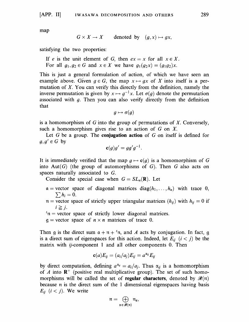
[APP. II] IW ASA W A DECOMPOSITION AND OTHERS
map GxX--tX denoted by (g, x) 1--+ gx,
satisfying the two properties:
If e is the unit element of G, then ex == x for all x EX. For all gl,g2 E G and x E X we have gl(g2X) == (glg2)X.
289
This is just a general formulation of action, of which we have seen an example above. Given g E G, the map x 1--+ gx of X into itself is a permutation of X. You can verify this directly from the definition, namely the inverse permutation is given by x 1--+ g-l x. Let a(g) denote the permutation associated with g. Then you can also verify directly from the definition that
g 1--+ a(g)
is a homomorphism of G into the group of permutations of X. Conversely, such a homomorphism gives rise to an action of G on X.
Let G be a group. The conjugation action of G on itself is defined for g,g'EGby
c(g)g' == gg' g-l .
It is immediately verified that the map g 1--+ c(g) is a homomorphism of G into Aut( G) (the group of automorphisms of G). Then G also acts on spaces naturally associated to G.
Consider the special case when G == SLn (R). Let
a == vector space of diagonal matrices diag(h 1, •.. , hn ) with trace 0, Lhi == O.
n == vector space of strictly upper triangular matrices (hij) with hij == 0 if i > j.
t n == vector space of strictly lower diagonal matrices. 9 == vector space of n x n matrices of trace O.
Then 9 is the direct sum a + n + tn, and A acts by conjugation. In fact, 9 is a direct sum of eigenspaces for this action. Indeed, let Eij (i < j) be the matrix with ij-component 1 and all other components O. Then
c(a)Eij == (ail aj )Eij == a(J.ij Eij
by direct computation, defining a(J.lj == ail aj. Thus lI.ij is a homomorphism of A into R+ (positive real multiplicative group). The set of such homomorphisms will be called the set of regular characters, denoted by 9l(n) because n is the direct sum of the 1 dimensional eigenspaces having basis Eij (i < j). We write
n == E9 n(J., (J.E~(n)
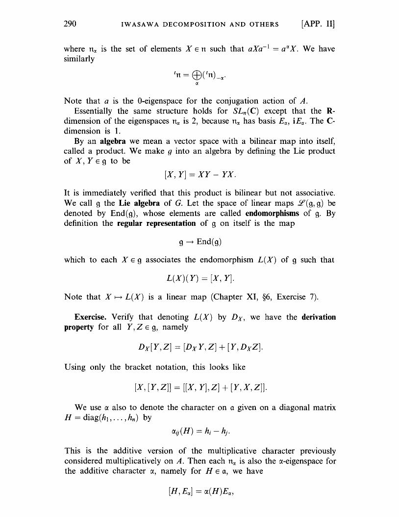
290 IW ASA W A DECOMPOSITION AND OTHERS [APP. II]
where noc is the set of elements X E n such that aXa- 1 == aOC X. We have similarly
Note that a is the O-eigenspace for the conjugation action of A. Essentially the same structure holds for SLn(C) except that the R
dimension of the eigenspaces noc is 2, because noc has basis EiJ.' iEiJ.. The Cdimension is 1.
By an algebra we mean a vector space with a bilinear map into itself, called a product. We make g into an algebra by defining the Lie product of X, Y E 9 to be
[X, Y] == XY - YX.
It is immediately verified that this product is bilinear but not associative. We call 9 the Lie algebra of G. Let the space of linear maps 2(g, g) be denoted by End(g), whose elements are called endomorphisms of g. By definition the regular representation of 9 on itself is the map
9 ~ End(g)
which to each X E 9 associates the endomorphism L(X) of 9 such that
L(X)( Y) == [X, Y].
Note that X ~ L(X) is a linear map (Chapter XI, §6, Exercise 7).
Exercise. Verify that denoting L(X) by Dx , we have the derivation property for all Y, Z E g, namely
Dx[Y,Z] == [DxY,Z] + [Y,DxZ].
Using only the bracket notation, this looks like
[X, [Y,Z]] == [[X, Y],Z] + [Y,X,Z]].
We use a also to denote the character on ° given on a diagonal matrix 11 == diag(h1, ... ,hn ) by
This is the additive version of the multiplicative character previously considered multiplicatively on A. Then each noc is also the a-eigenspace for the additive character a, namely for 11 E 0, we have
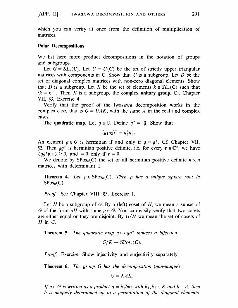
[APP. II] IW ASA W A DECOMPOSITION AND OTHERS 291
which you can verify at once from the definition of multiplication of matrices.
Polar Decompositions
We list here more product decompositions in the notation of groups and subgroups.
Let G == SLn ( C). Let U == U (C) be the set of strictly upper triangular matrices with components in C. Show that U is a subgroup. Let D be the set of diagonal complex matrices with non-zero diagonal elements. Show that D is a subgroup. Let K be the set of elements k E SLn(C) such that II( == k- l . Then K is a subgroup, the complex unitary group. Cf. Chapter VII, §3, Exercise 4.
Verify that the proof of the Iwasawa decomposition works in the complex case, that is G == UAK, with the same A in the real and complex cases.
The quadratic map. Let g E G. Define g* == I g. Show that
(glg2)* == g~g~.
An element g EGis hermitian if and only if g == g*. Cf. Chapter VII, §2. Then gg* is hermitian positive definite, i.e. for every v E Cn, we have <gg*v, v) > 0, and == ° only if v == 0.
We denote by SPosn(C) the set of all hermitian positive definite n x n matrices with determinant 1.
Theorem 4. Let p E SPosn(C). Then p has a unique square root in SPOsn(C).
Proof See Chapter VIII, §5, Exercise 1.
Let H be a subgroup of G. By a (left) coset of H, we mean a subset of G of the form gH with some g E G. You can easily verify that two cosets are either equal or they are disjoint. By G / H we mean the set of co sets of H in G.
Theorem 5. The quadratic map g ~ gg* induces a bijection
G/ K ~ SPosn(C).
Proof Exercise. Show injectivity and surjectivity separately.
Theorem 6. The group G has the decomposition (non-unique)
G == KAK.
If g EGis written as a product g == kl bk2 with kl' k2 E K and b E A, then b is uniquely determined up to a permutation of the diagonal elements.
292 IW ASA W A DECOMPOSITION AND OTHERS [APP. II]
Proof Given g E G there exists kl E K and b E A such that
by using Chapter VIII, Theorem 4.4. By the bijection of Theorem 5, there exists k2 E K such that g == k 1bk2, which proves the existence of the decomposition. As to the uniqueness, note that b2 is the diagonal matrix of eigenvalues of gg*, i.e. the diagonal elements are the roots of the characteristic polynomial, and these roots are uniquely determined up to a permutation, thus proving the theorem.
Note that there is another version of the polar decomposition as follows.
Theorem 7. Abbreviate SPosn(C) == P. Then G == PK, and the decomposition of an element g == pk with PEP, k E K is unique.
Proof The existence is a rephrasing of Chapter VIII, §5, Exercise 4. As to uniqueness, suppose g == pk. The quadratic map gives gg* == pp* == p2. The uniqueness of the square root in Theorem 4 shows that p is uniquely determined by g, whence so is k, as was to be shown.
Index
A
Action 267, 286, 288 Adjoint 185 Algebra 290 Algebraically closed 279 Al terna ting 147 Anti1inear 128 Associated linear map 81 Associated matrix 82 Automorphism 288
B
Basis 11, 87 Bessel inequality 102 Bijective 48 Bilinear form 118, 132 Bilinear map 118, 132 Bounded from below 273 Bracket action 267
c Character 289 Characteristic polynomial 200, 206 Characteristic value 194 Coefficients of a matrix 29 Coefficients of a polynomial 232 Column 23 Column equivalence 161 Column rank 113 Column vector 24
Complex numbers 277 Complex unitary 291 Component 3, 99 Component of a matrix 23 Conjugate 278 Conjugation action 289 Constant term 232 Contained 1 Convex 77, 268 Convex closure 79 Coordinate functions 46 Coordinate vector 3, 11 Coordinates with respect to a basis 11 Coset 291 Cramer's rule 157 Cyclic 262
D
Degree of polynomial 232 Derivation property 290 Derivative 55, 129, 195 Determinant 140, 201 Diagonal elements 27 Diagonal matrix 27 Diagona1ize 93, 199, 218, 220, 221,
243 Differential equations 64, 197, 220,
258 Dimension 16, 20, 61, 66, 97, 106, 115 Dirac functional 127 Direct product 21
294 INDEX
Direct sum 19, 21, Ill, 257 Distance 98 Divide 250 Dot product 6, 31 Dual basis 127 Dual space 126
E
Eigencharacter 267 Eigenspace 195, 224 Eigenvalue 194, 201, 216 Eigenvector 194 Element 1 Endomorphism 289 Euclidean algorithm 245 Even permutation 168 Expansion of determinant 143, 149,
169 Extreme point 272
F
Fan 237 Fan basis 237 Field 2 Finite dimensional 17 Fourier coefficient 100, 109 Function space 7 Functional 126
G
Generate 6, 248 Gradient 129 Gram-Schmidt orthogonalization 104 Greatest common divisor 250 Group 283
H
Half space 269 Hamilton-Cayley 241 Hermitian form 184 Hermitian map 185, 225 Hermitian matrix 186 Hermitian product 108 Homomorphism 267, 288 Homogeneous equations 29 Hyperplane 269
I
Ideal 248 Identity map 48, 53
Image 60 Independent 10, 159 Index of nullity 137 Index of positivity 138 Infinite dimensional 17 Injective 47 Intersection 1 Invariant subspace 219, 237, 255,
260 Inverse 35, 48, 69, 163, 174, 283 Inverse image 80 Invertible 35, 87 Irreducible 251 Isomorphism 69 Isotropy group 286 Iwasawa decomposition 284
J
Jordan basis 263 Jordan normal form 264
K
Kernel 59 Krein-Milman theorem 275
L
Leading coefficient 232 Lie 267 Line 17, 57, 72 Linear combination 5 Linear equations 29, 113 Linear mapping 51, 54 Linearly dependent or independent
10, 86, 159, 160
M
M:, 88 Mapping 43 Markov matrix 240 Matrix 23, 81, 82, 88, 92, 120 Maximal set of linearly independent
elements 13, 17 Maximum 215 Minimal polynomial 254 Multilinear map 146 Multiplicity 253
N
Negative definite 224 Nilpotent 42, 94, 240
Non-degenerate 32, 95 Non-singular 35, 175 Non-trivial 29 Norm of a vector 97 Normal 227 Null form 137 Null space 124 Numbers 2
o Odd permutation 168 Operator 68, 181 Orthogonal 7, 96, 188 Orthogonal basis 103 Orthogonal complement 107, 130 Orthonormal 103, 110, 136
p
Parallelogram 58, 73, 99 Period 262 Permutation 163 Perpendicular 7, 96 Plane 17 Polar decomposition 292 Polarization 186 Polynomial 231 Positive definite operator 183 Positive definite product 97, 108,
222 Product 283 Product of determinants 172 Product of matrices 32 Projection 99 Proper subset 1 Pythagoras 99
Q
Quadratic map 291 Quadratic form 132, 214 Quaternions 287
R
Rank 114, 178 Real unitary 284 Reflection 199 Regular action 267 Regular characters 289 Regular representation 290
INDEX
Root 205, 233, 246 Rotation 85, 93 Row 23 Row rank 113
s Scalar product 6, 95 Schur's lemma 261 Schwarz inequality 100, 110 Segment 57, 72 Self-adjoint 185 Semilinear 128 Semipositive 183, 222, 226 Separating hyperplane 269 Sign of permutation 166 Similar matrices 93 Skew-symmetric 65, 183 Span 73, 75, 79 Spectral theorem 219, 226 Square matrix 24 Stable subspace 219 Strictly upper triangular 41 Subfield 2 Subgroup 284 Subset 1 Subspace 5 Sum of subspaces 9, 19 Supporting hyperplane 270 Surjective 48 Sylvester's theorem 137 Symmetric form 132 Symmetric linear map 182, 213 Symmetric matrix 26, 213
T
Trace 40, 64 Translation 49, 75 Transpose of linear map 182 Transpose of matrix 26, 37, 89 Transposition 164 Triangle 75 Triangle inequality 101 Triangulable 238 Triangular 28, 41 Trilinear 146 Trivial solution 29
u Union Unipotent 284, 285
295
296
Unique factorization 251 U nit element 283 Unit ideal 248 Unit sphere 215 Unit vector 99, 110 Unitary group 284, 291 Unitary map 188, 228, 243 Unitary matrix 27, 190 Unknown 29 Upper triangular 28, 41
INDEX
v Value 7 Vandermonde determinant 155 Vector 4 Vector space 3
z Zero mapping 53, 55 Zero matrix 25
Linear Algebra is intended for a one-term course at the junior or senior level. It begins with an exposition of the basic theory of vector spaces and proceeds to explain the fundamental structure theorems for linear maps, including eigenvectors and eigenvalues, quadratic and hermitian forms, diagonalization of symmetric, hermitian, and unitary linear maps and matrices, triangulation, and Jordan canonical form. The book also includes a useful chapter on convex sets and the finite-dimensional Krein-Milman theorem. The presentation is aimed at the student who has already had some exposure to the elementary theory of matrices, determinants, and linear maps. However the book is logically self-contained. In this new edition, many parts of the book have been rewritten and reorganized, and new exercises have been added.
sprtngeronllne.com
m
• Z
ISBN 0-387-96412-6
9


![Linear algebra [serge lang]](https://img.pdfslide.us/doc/110x75/557d0ff5d8b42a063b8b50ac/linear-algebra-serge-lang.jpg)