CHAPTER 11

QUANTUM MECHANICS

11.1. In conformity with the scope of this book, the emphasis of the present

chapter is on the mathematics of quantum mechanics, the physical ideas entering

the discussion only in a secondary way. Limitation of space further demands that

only the important, and this happily implies the more elementary, portions of the

wide field be presented. Complete exclusion of physical ideas would, however,

leave its subject matter so poorly joined and so incomprehensible to the student who

has no prior knowledge of quantum mechanics that the value of an entirely formal

treatment appears questionable. It is also true that no part of applied mathematics

exacts from its student a more radical change from his customary habits of thought,

a greater tolerance for new methods of inquiry, than does this latest branch. In order

to provide the proper attitude of mind, we preface the later mathematical

developments by a few qualitative remarks whose relevance to the present book is

but auxiliary.

The central notion of classical mechanics is the mass point, or particle.

Classical theory therefore presupposes, tacitly, that a physical system can in

principle be recognized as a particle, or a set of particles. Until the advent of

quantum physics this dogma has never been questioned; in fact scientific

philosophers have frequently inflated it to the dimensions of a universal proposition

claiming that all physical systems are composed of particles. The method of

physical description in best accord with this fundamental attitude is clearly this: To

correlate instantaneous positions of a given particle with instants of time, assuming

motion to be continuous in space and time. Thus, if a particle moves along the X-

axis, the complete description of its motion would appear in the form 𝑥 = 𝑓(𝑡).

Now it is conceivable that such a correlation becomes impossible, and the

question then arises whether this fundamental mode of description should be

abandoned in such circumstances. The answer which has often been given and

which the modern physicist emphatically rejects is the flatly negative one, the

answer alleging that classical description is intrinsically evident and that the relation

𝑥 = 𝑓(𝑡) has meaning even when the functional relation cannot be established. On

the other hand, one would not like to discard this successful description lightly, for

instance because of certain practical and accidental difficulties in the procedure of

measuring 𝑥 as a function of 𝑡. The criterion which has ultimately produced clarity

is this: A method of description must be abandoned when it becomes impossible,

not because of experimental difficulty, but because its use contradicts known laws

of science. Classical description has become impossible for the latter reason, as the

following simple example will show.

Imagine an oscillating mass point, e.g., the bob of a pendulum. As long as

the eye can follow the bob, correlations between x and t can certainly be made. But

suppose the mass point is made to increase its frequency of vibration. The eye will

soon be unable to perceive instantaneous positions, but the camera can still establish

them. when the camera fails, oscillographic methods may be available, and after

that, ingenious devices perhaps not yet invented may serve. But ultimately, a barrier

of an essential kind will be encountered. Let us assume that the bob oscillates 1010

times per second. It is a fact of atomic physics that visible light requires about 10−8

seconds to be emitted (or reflected). Thus if it were used as the medium of report,

the light-emitting mass would have to remain in a given position for approximately

that length of time. In the present instance, however, the bob executes 100

vibrations within this period. A similar argument can finally be used to invalidate

every other means for establishing the classical correspondence. The latter has to

be ultimately abandoned because its use contradicts the laws of optics.

What, then, can be done? Perhaps the example suggests an answer. While a

snapshot can in principle no longer be taken of the rapidly oscillating bob, a time

exposure would reveal some features of its dynamical b behavior. It would give

essentially a correlation between the time the bob spends within a given interval dx

and the location of that interval, in other words between x and the probability wdx

of encountering it in dx. This leads to a less pretentious description of the physical

system called a mass point, of the form w= p (x), and this description is characteristic

of quantum mechanics. It is to be noted that p (x) can be inferred from the classical

relation 𝑥 = 𝑓(𝑡), but not ,𝑓(𝑡) from 𝑤 = 𝑝(𝑥).

Quantum mechanics provides the means for deducing probability relations

of the type described, and it does so in a logically consistent fashion. But before

turning to this central issue, let us see what has become of the concept: particle. Our

time exposure has left it very ill defined. Indeed if the system called a mass point

were invisibly small or never sufficiently stationary to permit the classical

description, the customary properties of particles would never be exhibited. By the

criterion of essential observability, the concept would lose its physical significance.

From a misunderstanding of this situation there has arisen a claim that quantum

mechanics leads to a dualism, to the monstrous conception that ultimate entities of

physics like electrons are both particles and waves; the correct statement is that they

are neither particles nor waves, but more abstract entities for the description of

which quantum mechanics gives most simple and successful rules. The question as

to the particle or wave nature of an electron must be put in the same class as that

regarding its color or, to use a lighter metaphor due to the philosopher Dingle, as

the question concerning the color of an elephant’s egg if an elephant laid eggs.

Despite this fundamental situation we shall place no ban upon the use of the

terms particle, wave, etc.; we shall even adhere to universal practice in calling the

electron one of the elementary particles of nature; we do this only, of course, as a

concession to usage. But whenever a paradox arises, the reader should endeavor to

resolve it by recalling that the “classical language” when applied to atomic entities

is in fact metaphoric.

AXIOMATIC FOUNDATION

11.2. Definitions.

For the sake of brevity all historical considerations are omitted here. Nor

will any attempt be made to “deduce” quantum mechanics either from classical

physics or from outstanding experimental facts, for in a strict logical sense this

cannot be done. We shall, however, present the framework of the theory with utmost

economy of thought and space, committing the reader to the tacit understanding that

all experimental consequences of the theory outlined have been verified as far as

they could hitherto be tested.

On a physical system, by which is meant any object of interest to physic or

chemistry, numerous observation or measurements can be made. The quantities so

observed or measured, such as size, energy, position and momentum, are called

observables. It is well to think of these observables without ascribing to them the

intuitive qualities they possess in classical mechanics. Position, or energy, is not so

much possessed by a system as it is characteristic of a certain measuring process

which can be carried out upon it. The measurement of an observable upon a system

yield a number.

In defining the state of a physical system considerable caution must be

exercised, for we wish to remain in keeping with the requirements outlined in the

introductory paragraphs. First it is well to notice that by state the scientist never

means anything not subject to arbitrary fixation; indeed the definition of state is

made to conform to the needs of each particular subject. It is quite different, for

instance, in classical mechanics from what it is in thermodynamics or in

electrodynamics. Hence we need not feel ill at ease when in quantum mechanics a

new choice is made. Leaving elucidation until later: a state is1 a function of certain

variables, a function from which by the rules of quantum theory significant

1 The reader who dislike this phrase may substitute “is represented by” for the simple “is”. We

wish to warn, however, that the spirit of quantum mechanics permits no distinction in meaning

between these two expressions.

information can be obtained. The variables may be chosen in several ways, each

giving rise to a consistent description equivalent to all others; here they will be

taken to be space coordinates, for this gives rise to the form of quantum mechanics

most commonly used, namely Schrodinger’s. By state function, we thus mean a

mathematical construct, ∅(𝑥1, 𝑦1, 𝑧1; 𝑥2, 𝑦2, 𝑧2; … 𝑥𝑛, 𝑦𝑛, 𝑧𝑛). It is possible, as we

shall later see, to associate the variables 𝑥1 . . . 𝑧𝑛 with the dimensions of

configuration space of the classical analogue of the system in question. In particular,

the number of variables needed in ∅ for a complete description of its behavior (at

a given instant of time) has always been found to be equal to the number of its

classical degrees of freedom. This must indeed be the case in order that large scale

bodies be consistently described both by quantum mechanics and by classical

mechanics. States may change with time; hence a state in its widest meaning may

be written

∅(𝑥1𝑦1𝑧1…𝑧𝑛, 𝑡)

Certain restrictions are to be placed upon state functions, restrictions which

will take on greater plausibility in view of the postulates of the next section. Most

important among them are two: first ∅, which may be a complex function, must

possess an integrable square2 in the sense that

∫∅ ∗ ∅𝑑𝜏 < ∞ (11-1)

Where 𝑑𝜏 is the “Volume of configuration space,” i.e., in rectangular

coordinates

𝑑𝜏 ≡ 𝑑𝑥1𝑑𝑦1𝑑𝑧 . . . 𝑑1𝑑𝑥𝑛𝑑𝑦𝑛𝑑𝑧𝑛

Second,

2 This statement requires modification in some cases. See remarks concerning “continuous

spectrum,” sec. 11.9c. Condition (1) must be rigorously maintained without exception when ∫ 𝑑𝜏 is

finite. It seems best to present the foundations of the theory with this restriction., leaving necessary

generalizations for later

∅ is single − valued (11-2)

The function ∅ may of course be expressed in any other system of space

coordinates by the ordinary geometric transformations of Chapter 5. Condition (2)

is particularly important when one of the variables is an angle, say 𝛼, for it then

requires that

∅ (𝛼) = ∅ (𝛼 + 2𝑛𝜋) (11-3)

𝑛 being an integer

Finally we must include in our list of definitions another mathematical

construct, that of an operator. Every specific mathematical operation, like adding

6, or multiplying by c, or extracting the third root, etc., can be represented by a

characteristic symbol which is then called an operator. Operators are:

6+, 𝑐. , √3

,𝑑

𝑑𝑥 , ∫ 𝑑𝑡

𝑏

𝑎, 𝐴

𝑑2

𝑑𝑥2+ 𝐵

𝑑

𝑑𝑥+ 𝐶, and so forth. In general they act on

functions. They can be applied in succession. When they are so applied, the order

in which the operators occur is important. For convenience, let us use more general

symbols for operators, such as P and Q. If P stands for + and Q for c., then PQF

means 𝛼 + 𝑐𝑓 𝑤ℎ𝑒𝑟𝑒 𝑓 is a function; however QPf means c ( + f ). Thus

QPf = PQf + ( c – 1 ) (11-4)

Such an equation is said to be an operator equation. The reader will at once

verify that, if P stands for / x and Q for x., the operator equation

PQf - QPf = f (11-5)

There is an important difference between eqs. (4) and (5); the second is

homogeneous in f, the first is not. From the second, f may be canceled symbolically

so that it reads

PQ – QP = 1 (11-5)

Only homogeneous operator equations of this kind, usually written in the

latter form without explicit insertion of the operand f, are of interest in quantum

mechanics.

The formalism of operator is convenient also in other ways. It is possible,

for instance, to define a periodic function ∅ (𝑥) by writing

𝑒ℎ𝐷∅ (𝑥) = ∅ (𝑥)

D being d/dx; for the left-hand side is, on expansion, simply the Taylor

series for ∅ (𝑥 + ℎ).

Two operators, P and Q, are said to commute when PQ – QP is zero. Thus

c and d/dx; commute if c is a constant. Other examples of commuting operators

are: x and d/dx; d/dx and ∫ 𝑑𝑥𝑏

𝑎 if and b are constant; + and ( b ). Clearly,

every operator commutes with itself or any power of itself, provided that by the n-

th power we mean the n-fold iteration of the operator.

11.3. Postulates.3

a. The fundamental postulates of quantum mechanics are three in number.

The first concerns the use of observables.

Brief reflection will show that classical physics associates with observables

certain definite function of suitable variables: x, y, z with position, mv with linear

momentum, 1

2𝑚𝑣2 with kinetic energy, and so forth. These function are chosen to

describe experience most adequately. There is no logical reason which would

exclude the use of more abstract mathematical entities in this association. It has

3 Henceforth in the present section, and in all subsequent sections up to 11.25, states will be

supposed to be independent of the time; i.e., ∅ does not contain I, Such states are known as

stationary ones, and the part of quantum mechanics dealing with them will be called quantum

statics. In quantum dynamics, introduced in sec. 11.25, a new postulate (Schrodinger’s “time”

equation) will be needed. This postulate is not included in the present list. Nor do we include the

Pauli principle, which is also of axiomatic status, and which will be presented in sec. 11.33. The

presented limitation is made for pedagogical reasons

indeed been found that, for the description of atomic phenomena, certain operators

should replace the functions which in classical mechanics represent observables.

The first postulate may be stated as follows:

To every observable there corresponds an operator.

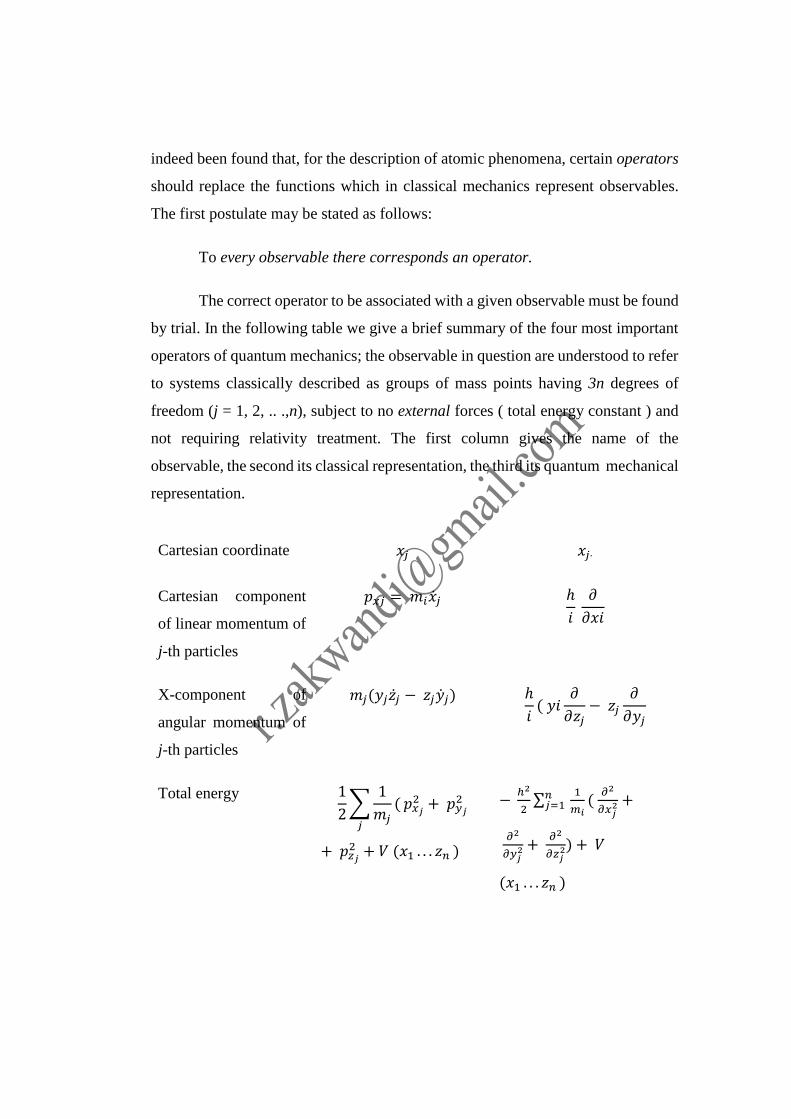
The correct operator to be associated with a given observable must be found

by trial. In the following table we give a brief summary of the four most important

operators of quantum mechanics; the observable in question are understood to refer

to systems classically described as groups of mass points having 3n degrees of

freedom (j = 1, 2, .. .,n), subject to no external forces ( total energy constant ) and

not requiring relativity treatment. The first column gives the name of the

observable, the second its classical representation, the third its quantum mechanical

representation.

Cartesian coordinate 𝑥𝑗 𝑥𝑗

Cartesian component

of linear momentum of

j-th particles

𝑝𝑥𝑗 = 𝑚𝑖��𝑗 ℎ

𝑖 𝜕

𝜕𝑥𝑖

X-component of

angular momentum of

j-th particles

𝑚𝑗(𝑦𝑗��𝑗 − 𝑧𝑗��𝑗) ℎ

𝑖( 𝑦𝑖

𝜕

𝜕𝑧𝑗− 𝑧𝑗

𝜕

𝜕𝑦𝑗

Total energy 1

2∑

1

𝑚𝑗(

𝑗

𝑝𝑥𝑗2 + 𝑝𝑦𝑗

2

+ 𝑝𝑧𝑗2 + 𝑉 (𝑥1 . . . 𝑧𝑛 )

− ℎ2

2∑

1

𝑚𝑖( 𝜕2

𝜕𝑥𝑗2 +

𝑛𝑗=1

𝜕2

𝜕𝑦𝑗2 +

𝜕2

𝜕𝑧𝑗2) + 𝑉

(𝑥1 . . . 𝑧𝑛 )

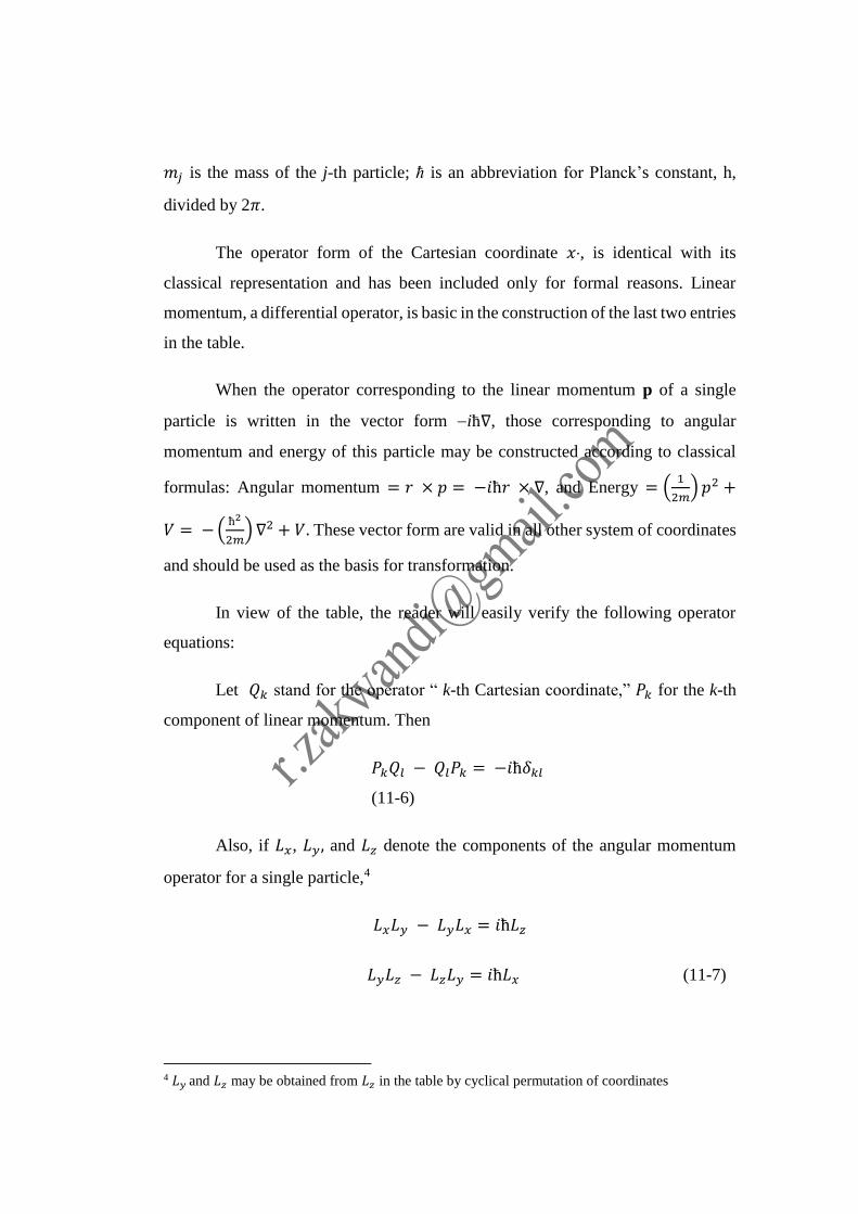
𝑚𝑗 is the mass of the j-th particle; ћ is an abbreviation for Planck’s constant, h,

divided by 2𝜋.

The operator form of the Cartesian coordinate 𝑥, is identical with its

classical representation and has been included only for formal reasons. Linear

momentum, a differential operator, is basic in the construction of the last two entries

in the table.

When the operator corresponding to the linear momentum p of a single

particle is written in the vector form iћ∇, those corresponding to angular

momentum and energy of this particle may be constructed according to classical

formulas: Angular momentum = 𝑟 × 𝑝 = −𝑖ћ𝑟 × ∇, and Energy = (1

2𝑚) 𝑝2 +

𝑉 = −(ћ2

2𝑚) ∇2 + 𝑉. These vector form are valid in all other system of coordinates

and should be used as the basis for transformation.

In view of the table, the reader will easily verify the following operator

equations:

Let 𝑄𝑘 stand for the operator “ k-th Cartesian coordinate,” 𝑃𝑘 for the k-th

component of linear momentum. Then

𝑃𝑘𝑄𝑙 − 𝑄𝑙𝑃𝑘 = −𝑖ћ𝛿𝑘𝑙

(11-6)

Also, if 𝐿𝑥, 𝐿𝑦, and 𝐿𝑧 denote the components of the angular momentum

operator for a single particle,4

𝐿𝑥𝐿𝑦 − 𝐿𝑦𝐿𝑥 = 𝑖ћ𝐿𝑧

𝐿𝑦𝐿𝑧 − 𝐿𝑧𝐿𝑦 = 𝑖ћ𝐿𝑥 (11-7)

4 𝐿𝑦 and 𝐿𝑧 may be obtained from 𝐿𝑧 in the table by cyclical permutation of coordinates

𝐿𝑧𝐿𝑥 − 𝐿𝑥𝐿𝑧 = 𝑖ћ𝐿𝑦

Commutation rules, like (6) and (7), are often sufficient to define the

operators involved without recourse to their explicit form, but the latter is usually

helpful.

b. The second postulate states:

The only possible values which a measurement of the observable whose

operator is P can yield are the eigenvalues pλ of the equation

𝑃𝜓𝜆 = 𝑝𝜆𝜓𝜆 (11-8)

Provided 𝜓𝜆 obeys conditions (1) and (2),namely: ∫𝜓𝜆∗ 𝜓𝜆𝑑𝜏 <

∞ 𝑎𝑛𝑑 𝜓𝜆 is single-valued.

The range of integration depends on the particular problem under

consideration, as will be seen later.

We illustrate the meaning of this postulate by a few examples. Let us find

the measurable values of the linear momentum of a particle, known to be

somewhere on the X-axis between the finite points 𝑥 = 𝛼 and 𝑥 = 𝑏. The operator

P is −𝑖ћ (𝜕

𝜕𝑥). Eq. (8) therefore becomes a first-order differential equation which

can obviously be satisfied if 𝜓𝜆 is assumed to be a function of x only. It reads

−𝑖ћ𝑑𝜓𝜆

𝑑𝑥= 𝑝𝜆𝜓𝜆 (11-9)

And has the solution

𝜓𝜆 = 𝑐𝑒(𝑖ћ)𝑝𝜆𝑥

is this solution satisfactory from the point of view of eqs. (1) and (2) ? It is certainly

single-valued; moreover, ∫ѱ𝜆∗ ѱ𝜆𝑑𝑥 = (𝑏 − 𝑎)𝑐

∗𝑐 is finite for every finite c.

Hence bo restriction upon 𝑝𝜆 results; 𝑎𝑙𝑙 values of the linear momentum may be

found upon measurement. The eigenvalues of the linear momentum from a

continuous spectrum ( λ is not a discrete index) and every function of the form

𝑐𝑒(𝑖

ћ)𝑝𝑥

with constant 𝑝 is an eigenfunction. As far as measurable values of linear

momentum are concerned, quantum mechanics leads to the same result as classical

physics.

This in not true for the 𝑎𝑛𝑔𝑢𝑙𝑎𝑟 momentum of a single particle. Here eq.

(8) reads

−𝑖ћ (𝑥𝜕

𝜕𝑦− 𝑦

𝜕

𝜕𝑥)ѱ𝜆 = 𝑚𝜆𝜓𝜆 (11-10)

Provided we consider the 𝑧-component and write ѱ𝜆 for the eigenvalues.

Obviously, ѱ𝜆 must be a fuction of both x and y. But a simple transformation of

coordinates reduces the equantion to a simpler form. On putting 𝑥 = 𝑟 cos 𝜃 and

𝑦 = 𝑟 sin 𝜃 , we have

𝑑

𝑑𝜃= −𝑟 sin 𝜃

𝜕

𝜕𝑥+ 𝑟 cos 𝜃

𝜕

𝜕𝑦= 𝑥

𝜕

𝜕𝑦− 𝑦

𝜕

𝜕𝑦

Therefore aq. (10) becomes

−𝑖ћ 𝑑ѱ𝜆𝑑𝜃

= 𝑚𝜆ѱ𝜆

And ѱ𝜆 is seen to be a funcition of 𝜃 alone. The solution is

ѱ𝜆 = 𝑐𝑒(𝑖ћ)𝑚𝜆𝜃

It certainly has an integrable square, because the range of 𝜃 extends from 0

to 2𝜋, or more exactly, from 2𝜋𝑛 to 2𝜋(𝑛 + 1), where 𝑛 is an integer. But ѱ𝜆

violates the condition of single-validness which must be imposed in the from (3).

To satisfy it we must require that

ѱ𝜆(𝜃) = ѱ𝜆(𝜃 + 2𝜋)

And this implies 𝑒(2𝜋𝑖

ћ)𝑚𝜆 = 1. This is true only if

𝑚𝜆 = 𝜆ћ , 𝜆 an integer (11-11)

Hence the only observable values of the angular momentum are given by

(11), and the eigenfunctions are 𝑐𝑒(𝑖

𝜃). This result is identical with the postulate of

the older Bohr theory concerning angular momentum.

Next we consider the possible values of the total energy of a single mass

point. The energy operator appearing in the table is often referred to as the

Hamiltonian operator and is denoted by the symbol H. let us use 𝐸𝜆 for the

eigenvalues. The operator equation then becomes

𝐻ѱ𝜆 ≡ −ћ2

2𝑚∇2ѱ𝜆 + 𝑉(𝑥, 𝑦, 𝑧)ѱ𝜆 = 𝐸𝜆ѱ𝜆 (11-12)

This equation, written perhaps more frequently in the form

∇2ѱ𝜆 + 2𝑚

ћ2 (𝐸𝜆 − 𝑉)ѱ𝜆 = 0 (11-12)

Was found by 𝑆𝑐ℎ𝑟��𝑑𝑖𝑛𝑔𝑒𝑟 and bears his name. Its solutions and eigen-values

clearly depend on the functional nature of 𝑉(𝑥, 𝑦, 𝑧); they will be reserved for

detailed consideration in secs. 9 et seq.

A rather peculiar result is obtained when (8) is applied to the coordinate

“operator”. The eigenvalues of “𝑥“ are the values ξ𝜆for which the equation

𝑥. ѱ𝜆 = ξ𝜆ѱ𝜆

an ordinary algebraic one, possesses solutions. On writing it in the form

(𝑥 − ξ𝜆)ѱ𝜆 = 0

It is evident that either 𝑥 = ξ𝜆 or ѱ𝜆 = 0. In plainer language, ѱ𝜆 as a function

of 𝑥 vanishes everywhere except at 𝑥 = ξ𝜆, a constant. From a rigorous

mathematical point of view such a function is a monstrosity, but it is useful for

certain purposes to introduce it, as Dirac5 has done. It is called 𝛿(𝑥 − ξ𝜆), the

symbol being fashioned after the Kronecker 𝛿, and is best visualized as something

like lim𝑎→0

𝑐𝑒−(𝑥−ξ𝜆)2/𝑎

. For later use the constant 𝑐(𝑎) will be so chose that

∫ 𝛿(𝑥 − 𝜉)𝑑𝑥 = 1,∞

−∞ so that

∫ 𝑓(𝑥)𝛿(𝑥 − 𝜉)𝑑𝑥 = 𝑓(𝜉)∞

−∞ (11-13)

now it is clear that such a “function” can be formed for every value ξ𝜆 , hence every

point of the X-axis is an eigenvalue of the 𝑥-coordinate. 6

The significance of the second postulate is best grasped when it is regarded

as furnishing a catalogue of the measurable values of all observables for which

operators are known. It implies no information concerning the meaning of the

eigenfunction ѱ𝜆. These are, of course, states of the system in the sense explained.

Their nature will unfold itself when the third postulate has been set forth. For the

present we only note that every 𝜓𝜆 is indeterminate with respect to a constant

multiplier; eq.(8) will also be satisfied by constant 𝜓𝜆 On the other hand,

∫𝜓𝜆∗𝜓𝜆 𝑑𝜏 exists. We may require, therefore, that 𝜓𝜆 is normalized after the manner

of sec.8.2. Henceforth this will be assumed unless a statement to the contrary is

made. In this connection it may be recalled, however, that normalization may fail

intrinsically when the eigenvalues 𝑝𝜆 form a continuous spectrum. In Chapter 8 this

was shown to be the case in instances where the range of the fundamental variable

became infinite. These require special treatment.

The 𝜓𝜆 will be orthogonal if operator and boundary conditions conform to

the circumstances of the Sturm- Liouville theory (sec.8.5). this theory, as will later

5 Dirac, P.A.M., “Principles of Quantum Mechanics,” Third Edition; Clarendon Press, Oxford, 1947.

6 The operation 𝑥. has continuous spectrum. Correspondingly , the integral ∫ 𝛿2(𝑥 − 𝜉)𝑑𝑥 does not

exist ! See ses. 11.9c.

be seen, covers most of the cases occurring in quantum mechanics, but must be

generalized somewhat to be applicable to complex operators.

c. We turn to the third postulate which states:

when a given system is in a state ∅, the expected means of a sequence of

measurements on the observable whose operator is P is given by

�� = ∫ ∅∗ 𝑃∅𝑑𝜏 (11-14)

The expected means is defined as in statistics : If a large number of

measurements is made on the system, and the measured values are 𝑝1,𝑝2,……..

𝑝𝑁 ,then �� ≡1

𝑁∑ 𝑃𝑖𝑁𝑖=1 . Note that eq. (14) does not predict the outcome of a single

measurement.

In writing (14) we are again supposing that ∅ is normalizes. This can be

brought about all physical problems by “confining” the system in configuration

space, that is, by taking the volume in which it moves to be finite, so that ∫𝑑𝜏

exists. Even if the volume is infinite, ∫∅ ∗ ∅𝑑𝜏 may still exist, but in general the

situation then calls for special treatment involving the use eigendifferentials instead

of eigenfunctions. * A more general form of eq. (14), which often works when the

volume of configuration space is infinite, is the following

�� = 𝑙𝑖𝑚𝜏 → ∞

∫𝜏 𝑃∅𝑑𝜏

∫𝜏∅∗∅𝑑𝜏

(11-14’)

*See Morse, P.M., and Feshbach, H., “Methods of Theoretical Physics,”MeGraw

Hill Book Co., Inc., 1953. We illustrate the meaning of (14) by a few examples.

Let a system having one degree of freedom be in a state described by∅ =

(𝑏/𝜋)1

4𝑒− (𝑏

2)(𝑥− 𝜉)2

. Then the mean value of its position will be:

�� = ∫ ∅2𝑥𝑑𝑥 = 𝜉∞

−∞

Its mean momentum:

��𝑥 = −𝑖ћ ∫∅∅′𝑑𝑥 = 0

Its mean kinetic energy:

��𝑘𝑖𝑛 = −ћ2

2𝑚∫∅∅′′𝑑𝑥 =

ћ2

2𝑚∫(∅′)2 𝑑𝑥 =

𝑏

2 ∙ ћ2

2𝑚

It is interesting to note that, the more concentrated the function ∅ (the

greater b) the larger will be the mean kinetic energy. To calculate the mean total

energy we should have to know the form of 𝑉 (𝑥).

Let us take ∅ = 𝑒𝑖𝑘𝑥 / (b – a)1/2 . We then find

�� = ∫ ∅∗𝑥∅𝑑𝑥 = 𝑏 + 𝑎

2

𝑏

𝑎

��𝑥 = −𝑖ћ∫ ∅∗∅′𝑑𝑥 = 𝑘ℎ𝑏

𝑎

��𝑘𝑖𝑛 = −ℎ2

2𝑚 ∫ ∅∗∅′′𝑑𝑥 =

𝑘2ℎ2

2𝑚

𝑏

𝑎

If in this example the range is extended to infinity, let us say in such a way

that − 𝑎 = 𝑏 → ∞, the function 𝑒𝑖𝑘𝑥 can clearly not be normalized One just then

eq. (14’) in the form

�� = lim→∞

∫ ∅∗𝑝∅𝑑𝑥𝑎

−𝑎

∫ ∅∗∅𝑑𝑥𝑎

−𝑎

Which gives the same result as those obtained above.

The three postulates here stated and exemplified do not reveal an intuitive

meaning of the state function ∅. It is therefore not unusual in textbooks on quantum

mechanics to add another postulate stating that ∅∗(𝑥)∅(𝑥) signifies the probability

that the “particle” whose state is ∅ be found at the point 𝑥 of configuration space (

with suitable generalization for more than one degree of freedom). This is indeed

true, and it may be well for the reader to form this basic conception; but this

statement is not a further postulate since it may be deduced from those already

given.( Cf. sec.6. )

DEDUCTIONS FROM THE POSTULATES

11.4. Orthogonality and Completeness of Eigenfunctions.

In Chapter 8, orthogonality and completeness of the eigenfunctions belonging to

the Sturm-Liouville operator L have been discussed. The proofs there given need to

be generalized if they are to be applied to quantum mechanics, for the operators

occurring there are not all af the same structure as L. (one of the mist important

equations encountered, the one-dimensional Schr��dinger equantion (12), is of the

Sturm-Liouville type.) They often involve many variables, they may be differential

operators of the first order, they may be complex; in fact they may not be differential

operators at all. To simplify the theory we shall assume that the eigenvalues 𝑝𝜆 of

eq. (8) are discrete, and that the boundary conditions on acceptable state functions

are of the form 1 and 2. Whenever convenient we shall even assume that ∅ vanishes

at the boundary of configuration space, over which integrations are to be carried

out, in a manner suitable to our needs. Unless these restrictions are made the

arguments become involved and in some respects problematic. It would the be

necessary to conduct a separate proof for every problem of interest; thus elegance

would fall prey to rigor.

We first define what is meant by an Hermitian operator. Let u and v be two

“acceptable” functions, defined over a certain range of configuration space 𝜏. We

then say that the operator P in Hermituan if

∫𝜏𝑢∗ ∙ 𝑃𝑣𝑑𝜏 = ∫

𝜏𝑣 ∙ 𝑃∗𝑢∗𝑑𝜏 (11-15)

All operators of interest in quantum mechanics have property. As a sample

proof The hermitian property of 𝑥 . is obvious. To prove it for the Hamiltanian H,

two partial integrations are necessary; the details may be left as an exercise for the

reader.

Hermitian operators real eigenvalues. The fact follows at once from eq. (15)

the eigenvalues of P are defined by the equation.

𝑃ѱ𝜆 = 𝑝𝜆 ѱ𝜆 (11 − 16)

This also implies the validity of the equantion

𝑃∗ѱ𝜆∗ = 𝑝𝜆

∗ѱ𝜆 ∗ (11-17)

Now multiply (16) by ѱ𝜆 ∗ and (17) by ѱ𝜆 , and integrate over 𝑑𝜏 obtaining

∫ѱ𝜆∗ 𝑃ѱ𝜆𝑑𝜏 = 𝑝𝜆 ∫ѱ𝜆

∗ 𝑃ѱ𝜆𝑑𝜏 ∫ѱ𝜆𝑃∗ѱ𝜆

∗𝑑𝜏 = 𝑝𝜆∗∫ѱ𝜆

∗ 𝑃ѱ𝜆𝑑𝜏

By (15) the left-hand sides of these two equation are equal, for ѱ𝜆 is certainly an

acceptable function in the sense outlined before. Hence 𝑝𝜆∗ = 𝑝𝜆 ; i.e., 𝑝𝜆 is real.

Since the eigenvalues of operators are measurable values of observables, which

must of necessity be real, the physical significance of an operator is assured when

it has the Hermitian property.

Let us again consider eq. (16). If ѱ𝜇 is some other eigenfunction, it is

evident that

∫ѱ𝜇∗ 𝑃ѱ𝜆𝑑𝜏 = 𝑝𝜆 ∫ѱ𝜇

∗ 𝑃ѱ𝜆𝑑𝜏 (11-18)

But if we start with the equation

𝑃∗ѱ𝜇∗ = 𝑝𝜇ѱ𝜇

∗

Which in true because 𝑝𝜇 is real, we also conclude that

∫ѱ𝜆𝑃∗ѱ𝜇

∗ 𝑑𝜏 = 𝑝𝜇 ∫ѱ𝜇∗ 𝑃ѱ𝜆𝑑𝜏 (11-19)

Combining (18) and (19) we find

∫ѱ𝜇∗ 𝑃ѱ𝜆𝑑𝜏 − ∫ѱ𝜆𝑃

∗ѱ𝜇∗ 𝑑𝜏 = ( 𝑝𝜆 − 𝑝𝜇) ∫ѱ𝜇

∗ 𝑃ѱ𝜆𝑑𝜏

If P is Hermitian the left-hand side vanishes. Hence either 𝑝𝜆 = 𝑝𝜇 or

∫ѱ𝜇∗ 𝑃ѱ𝜆𝑑𝜏 = 0 . we see that eigenfunctions of Hermition operators, belonging to

different eigenvalues, are orthogonal.

The completeness of the eigenfunctions of all operators employed in

quantum mechanics is usually assumed. To the authors’ knowledge, Rigorous proof

has not been given. Since, however, our main interest will be in the Schrodinger

equation which is of the Sturm-Liou vile type, this point need not detain us further.

In the following we shall assume completeness of all ψλ whenever this property is

needed.

Problem. Show that the angular momentum operator 𝐿𝑧 = −𝑖ћ ( 𝜕/𝜕𝜃 ) is

Hermitian.

11.5. Relative Frequencies of Measured Values.

Important consequent can now be deduced from the third postulate, eq. (14). We

first note that, if P is Hermitian, every power of P is Hermitian. Moreover, if (14)

is true for every operator P, it must certainly hold for the operator𝑃𝑟. It implies,

therefore,

𝑃𝑟 = ∫∅∗ 𝑃𝑟∅𝑑𝜏, 𝑟 = 1, 2, … (11-20)

The left-hand side stands, of course, foe the r-th moment of the statistical

aggregate or the measured values, i.e.,

𝑃𝑟 = ∑ 𝜌𝑖𝑖 𝑝𝑖𝑟 (11-21)

Provided 𝜌𝑖 is the relative frequency of the occurrence of the i-th eigenvalue 𝑝𝑖 in

the sett of measurement. In accordance with eq. (20), the state function ∅ predict

not only the mean, but all moments of the aggregate of measurements.7 Now eq.

(20) may be transformed as follows. Let the eigenfunctions of P be denoted by ѱλ,

7 for terminology., see sec. 12.3.

so that 𝑃ѱ𝜆 = 𝑝𝜆ѱ𝜆. On allowing P to operate on both side of this equations, there

result 𝑃2ѱ𝜆 = 𝑝𝜆𝑃ѱ𝜆 = 𝑝𝜆2ѱ𝜆. By continuing this process, the relation

𝑃𝑟ѱ𝜆 = 𝑝𝜆𝑟ѱ𝜆 (11-22)

Is established. If the function ∅ appearing in (20) is expanded in terms of the ѱ𝜆,

∅ = ∑𝑖ѱ𝑖𝑖

And this series is substituted, we find

𝑝𝑟 = ∫∑𝑖∗𝑗

𝑖𝑗

ѱ𝑖∗𝑃𝑟 ѱ𝑗𝑑𝜏 = ∑𝑖

∗𝑗𝑝𝑗𝑟

𝑖𝑗

∫ѱ𝑖∗ѱ𝑗 𝑑𝑑𝜏

= ∑𝑗∗𝑖𝑝𝑖

𝑟

𝑖

By virtue of (22) and the orthogonality of the ѱ𝑖. Comparing this with (21)

it is clear that

∑𝜌𝑖𝑝𝑖𝑟

𝑖

= ∑|𝑖|2𝑝𝑖

𝑟

𝑖

For every integer r. But this can be true only if

𝜌𝑖 = |𝑖|2 (11-23)

In Words: when the system is in the state ∅, a measurement of the

observable corresponding to P will yield the value 𝑝𝑖 with a probability (relative

frequency) |𝑖|2,𝑖 being the coefficient of ѱi in the expansion ∑ 𝜆ѱ𝜆,𝜆 and ѱ𝜆

is one of the eigenfunctions of P. The coefficients 𝑖 are called probability

amplitudes.

They may be expressed on terms of ∅ and ѱ𝑖 by the relation

∫ѱ𝑖∗∅𝑑𝜏 = ∑ ѱ𝑖

∗𝜆 𝜆ѱ𝜆𝑑𝜏 = 𝑖 (11-24)

Consequently, eq. (23) may also be written

𝜌𝑖 = | ∫ѱ𝑖∗∅𝑑𝜏|2 (11-25)

An interesting result is obtained when, in this equation, we let ∅ be one of

the eigenfunctions belonging to the operator P itself, e.g., ѱj. It then reads

𝜌𝑖 = | ∫ѱ𝑖∗∅𝑑𝜏|2 = 𝛿𝑖𝑗

All relative frequencies are zero expect the one measuring the occurrence of

the eigenvalue𝑝𝑗, which is unity. Thus we conclude that an Eigen state ѱ𝑗 of an

operator P is a state in which the system yields with certainly t5he value 𝑝𝑗 when

the observable corresponding to P is measured. Eigen functions are simply state

functions of this determinate character.

11.6. Intuitive Meaning of a State Function.

Consider now a system, like a simple mass point with one degree of

freedom, whose state function is ∅(𝑥). We wish to know the probability that a

measurement of its position will give the value 𝑥 = 𝜉. The eigenfunction

corresponding to the operator 𝑥 for the value ξ has been shown to be

ѱ𝜉 = 𝛿 (𝑥 − 𝜉)

Eq. (25) now reads

𝜌𝜉 = | ∫ 𝛿 (𝑥 − 𝜉) ∅(𝑥)𝑑𝑥 |2 = |∅(𝜉)|2 (11-26)

By virtue of (13). The probability (destiny) of finding the system at ξ is

given by the square of its state function. This fact provides a simple intuitive

meaning for the state function. It can be generalized to several dimensions Let

𝑞1, 𝑞2, . . . , 𝑞𝑛 be the coordinates on which ∅ depends. Using the former argument,

the eigenfunction corresponding to t5he composite coordinate operator 𝑞1 ∙ 𝑞2 ∙ ∙ ∙ ∙

𝑞𝑛 may be shown to be

ѱ𝜉1𝜉2∙∙∙𝜉𝑛 = 𝛿(𝑞1 − 𝜉1)𝛿(𝑞2 − 𝜉2)𝛿(𝑞𝑛 − 𝜉𝑛) (11-27)

If, therefore, we wish to find the probability 𝜌𝜉1𝜉2∙∙∙𝜉𝑛 of finding the system at the

point (𝜉1𝜉2 𝜉𝑛) of configuration space, we must use eq. (25) with ѱ𝑖 replaced by

(27). Hence

𝜌𝜉1∙∙∙𝜉𝑛 =

|∬∙∙∙ ∫ 𝛿 (𝑞1 − 𝜉1) ∙∙∙ 𝛿 (𝑞𝑛 − 𝜉𝑛)∅(𝑞1𝑞2 𝑞𝑛)𝑑𝑞1𝑑𝑞2 ∙∙∙ 𝑑𝑞𝑛|2 =

|∅(𝜉1𝜉2 𝜉𝑛)|2

11.7. Commuting Operators.

Let P and R be two operators satisfying the relation PR – RP = 0, and let

their eigenfunctions be ѱ𝜆 and𝑥𝜇, that is

𝑃ѱ𝜆 = 𝑝𝜆ѱ𝜆, 𝑅𝑥𝜇 = 𝑟𝜇𝑥𝜇 (11-28)

We assume the state function to be ѱ𝑖 so that, when P is measured, there result with

certainty the value𝑝𝑖. But

𝑅𝑃ѱ𝑖 = 𝑅𝑃ѱ𝑖 = 𝑝𝑖𝑅ѱ𝑖

Considering only the last two members of this equation, we may say that

(𝑅ѱ𝑖) is an eigenfunction of P, namely that belonging to the eigenvalue𝑝𝑖. But this

is possible only if 𝑅ѱ𝑖 = const. ѱ𝑖. Comparison with the second equation (28)

shows the constant to be one of the𝑟𝜇, and ѱ𝑖 to be one of the eigenfunction𝑥𝜇. We

conclude that commuting operators have simultaneous eigenstates; i.e.,

measurements on their observable yield definite values for both; they do not

“spread.”

The fact that, when P and Q are non-commuting operators and the state of

the system is an eigenstate of P, measurement on Q will give a statistical aggregate

of values and not a single one with certainty, is usually attributed to the interference

of measuring devices. For instance, the measurement of a particle’s position

disturbs its momentum, and vice versa, so that when one is ascertained with

precision, the other quantity loses it. From this point of view, measurements on the

observables associated with commuting operators are said to be compatible, the

procedures of measurements do not conflict do not conflict with each other.

11.8. Uncertainty Relation.

The proof of the famous Heisenberg uncertainty principle which will now

be given requires the use of an inequality, similar to a well known relation due to

Schwarz, though not identical with it. (Cf. eq. 3-112.)

Functions in the sense specified in connection with the definition of Hermitian

operators (sec. 11.4), then

∫𝑢∗𝑢𝑑𝜏 ∙ ∫ 𝑣∗𝑣𝑑𝜏 ≧1

4[∫(𝑢∗𝑣 + 𝑣∗𝑢)𝑑𝜏]2 (11-29)

We assume a system to be in a state∅, which need not be an eigenstate of

any particular operator, and we are interested in the result of measurements on the

observables belonging to two operators, P and Q, at present unspecified. Introduce

into eq. (29) the following functions

𝑢 = (𝑃 + ��)∅ 𝑎𝑛𝑑 𝑣 = 𝑖(𝑄 − ��)∅

Where �� and �� are mean values associated with P and Q through the relation (14).

Eq. (29) then reads

∫( 𝑃 − �� )∗∅∗(𝑃 − �� )∅𝑑𝜏 ∙ ∫(𝑄 − ��)∗∅∗(𝑄 − ��)∅𝑑𝜏 ≧

1

4[ 𝑖 ∫(𝑃 − ��)∗∅∗(𝑄 − ��)∅𝑑𝜏 − 𝑖 ∫(𝑄 − ��)∗ ∅∗(𝑃 − ��)∅𝑑𝜏]2

Now P and Q are Hermitian and satisfy eq. (15); �� and �� are constants. Therefore

the inequality reduce to

∫∅∗ ( 𝑃 − �� )2∅𝑑𝜏 ∙ ∫ ∅∗(𝑄 − ��)2 ∅𝑑𝜏 ≧ −1

4[∫∅∗(𝑃𝑄 − 𝑄𝑃)∅𝑑𝜏]2 (11-30)

Let us consider the meaning of the quantity ∫∅∗ ( 𝑃 − �� )2∅𝑑𝜏. When ∅ is

expanded in eigenfunctions ѱλ of P, ∅ = ∑ 𝜆ѱ𝜆𝜆 , and the expansion is introduced

in the integral, the result is ∑ |𝜆|2(𝑝𝜆 − 𝜆 ��)2, and this, in view of eq. (23),is

nothing other than the dispersion8 of the statistical aggregate of p-measurements

about their mean. For this quantity we may introduce the more familiar symbol∆𝑝2 .

A similar identification is to be made for∫∅∗(𝑄 − ��)2 ∅𝑑𝜏. Inequality (30) then

takes the more interesting form

∆𝑝2 . ∆𝑞2 ≧ −1

4[∫∅∗(𝑃𝑄 − 𝑄𝑃)∅𝑑𝜏]2 (11-31)

Now if P and Q commute, the right-hand side is zero, and it is possible for

∆𝑝2 𝑜𝑟 ∆𝑞2 to be zero, or even for both to vanish. This state of affairs recalls the

result of sec. 7, which was that both p- and q-measurements could yield single

values without spread.

When P and Q do not commute, relation (31) sets a lower limit for the

product of the dispersions, often called uncertainties. Suppose, for instance, that P

is the operator− 𝑖ћ (𝜕

𝜕𝑞), the linear momentum associated with q, and Q stands for

the coordinate q. We then have

𝑃𝑄 − 𝑄𝑃 = 𝑖ћ (11-32)

When this is put into (31) the result is ∆𝑝2 ∙ ∆𝑞2 ≧ћ2

4 , or , written in terms of

standard deviations, 𝛿𝑝 and 𝛿𝑞

𝛿𝑝 ∙ 𝛿𝑞 ≧ ћ/2 (11-33)

This is Heisenberg’s uncertainly relation.

8 The “dispersion” is the square of the so-called “standard deviation.” It is an index of the “ spread”

of the measurements. See chapter 12.

Our result need not be east in the form of an inequality. It is indeed quite

possible to calculate both 𝛿𝑝 and 𝛿𝑞 separately and exactly when the state function

∅ is given, as the postulates show.

A slight generalization of the present conclusions is also possible. There

are other operators, such as 𝐿𝑧 and 𝜃 (ef. Eq. 10 et seq.) which also obey eq. (32).

In fact all quantities which are called canonically conjugate in classical physics9

have operators which satisfy it. (Later we shall see that energy and time belong to

this class.) For all these, the uncertainty relation in the form (33) is valid.

Problem. Show that, if the state function ∅ is an eigenfunctions of the

angular momentum operator 𝐿𝑧 corresponding to the eigenvalue 𝐿𝑧 the product of

𝛿𝑙𝑥 and 𝛿𝑙𝑦 is at least as great as (ћ/2) 𝑙𝑧

SCHR��DINGER EQUATIONS

Attention will now be given to the eigenvalues and eigenfaunctions of

the energy operator, that is, to the solutions of the various forms of the Schrὄdinger

equations, eq. (12)

11.9. free Mass Point.− The simplest example of a physical system is

the free mass point for which the potential energy V may be taken to be zero. In that

case eq. (12) reads

∇2ѱ + 𝑘2ѱ = 0 (11-34)

Provided we omit the subscript λ and write𝑘2 ≡ 2𝑚𝐸/ћ2. This quantity

𝑘2 has a rather simple classical significance which it is well to recognize at once.

For if E is the total energy of the particle, which is in this case purely kinetic,

then𝐸 =1

2𝑚𝑣2 = 𝑝2/2𝑚. Hence 𝑘 ≡

𝑝

ћ, 𝑝 being the classical momentum of the

particle. Note also that k has the dimension opf a reciprocal length.

Eq. (34) has already been solved in Chapter 7 (cf. eq. 7-33), where it appeared as

the space form of the wave equation. To select the proper solution, we must consider

the fundamental domain, 𝜏, of our problem. Here, a great number of possibilities

present themselves.

a. Enclosure is a Parallelepiped. If the particle is known to be within a

parallelepiped of side lengths 𝑙1, 𝑙2 and𝑙3 , then 𝜏 is this volume of space.

Moreover, since |ѱ(𝑥𝑦𝑧)|2 has already been identified as the probability of finding

the particle at the point 𝑥, 𝑦, 𝑧 this quantity must certainly be zero everywhere

outside 𝜏. For reasons of continuity (which can, by more expanded arguments, be

shown to result from our axioms) we require that|ѱ|2, and hence ѱ itself, shall

vanish on the boundaries of 𝜏 also. In view of this boundary condition, the solution

of (34) in rectangular coordinates, namely eq. 7-36, must be chosen, in more

explicit form it reads

ѱ = (𝐴1𝑒𝑖𝑘1𝑥 + 𝐵1𝑒

−𝑖𝑘1𝑥) (𝐴2𝑒𝑖𝑘2𝑦 + 𝐵2𝑒

−𝑖𝑘2𝑦)(𝐴3𝑒𝑖𝑘2𝑦 + 𝐵3𝑒

−𝑖𝑘2𝑦,

𝑘2 = 𝑘12 + 𝑘2

2 + 𝑘32

The origin of the parallelepiped may be taken in one corner. Vanishing

of ѱ at the boundary then requires:

𝐴𝑠 + 𝐵𝑠 = 0, 𝐴𝑠𝑒𝑖𝑘𝑠𝑙𝑠 + 𝐵𝑠𝑒

−𝑖𝑘𝑠𝑙𝑠 = 0, 𝑠 − 1 ,2 ,3

The first condition makes each parenthesis of ѱ a sine-function; the second implies

𝑘𝑠 = 𝑛𝑠𝜋

𝑙𝑠

Where 𝑛𝑠 is an integer. Hence

ѱ = 𝑐 sin(𝑛1𝜋

𝑙1𝑥) sin(

𝑛2𝜋

𝑙2𝑦) sin(

𝑛3𝜋

𝑙3𝑧) (11-35)

and

𝑘2 = (𝑛12

𝑙12 +

𝑛22

𝑙22 +

𝑛32

𝑙32 )𝜋

2

So that

𝐸 = 𝜋2ћ2

2𝑚[(𝑛1

𝑙1)2 + (

𝑛2

𝑙2)2 + (

𝑛3

𝑙3)2] (11-36)

If ψ is to be normalized, ∫ψ ∗ ψdxdydz = 1, and the constant c has the value

𝑐 = (8

𝑙1𝑙2𝑙3)

12⁄

= (8

𝜏)

12⁄

The permitted energy values form a denumerably infinite set. Their arrangement

is best represented by constructing a lattice of points filling all space, with the

“reciprocal” parallelepiped of sides 1 𝑙1⁄ , 1 𝑙2

⁄ , 1 𝑙1⁄ as crystallographyc unit. If

from a given point lines are drawn to all other points, the squares of the lengths of

these lines (multiplied by 𝜋2ℎ2/2m) are the energies of our problem. However, not

all these lines represent different states. The function ψ changes only it sign when

one of the integers 𝑛1, 𝑛2 𝑜𝑟 𝑛3 changes sign; it is not therebly converted into a new,

linearly independent function. Hence only the lines lying in one octant of the lattice,

with the origin of the lines at one corner, will represent different states. If some of

the𝑙′𝑠 are equal there will be degeneracy (cf. Sec. 8. 6), for then an interchange of

the corresponding 𝑛′𝑠 will not produce a different E, while ψ will be changed into

a function which is nearly independent from the original one.

b. Enclosure is s sphere. Eq. (34) must now be solved in sphericak

coordinates. But this has already been done in sec. 8.4 (cf. Eq. 8-25), for an

acoustical problem. The eigenfunctions are, aside from normalizing factorψ =

𝑌𝑙(𝜃, 𝜑)𝑟−1

2⁄ 𝐽𝑙+1

2

(𝑘𝑟). The permitted energies are determined by the condition

𝐽𝑙+

1

2

(𝑘𝑎) = 0 where 𝑎 is the radius of the enclosure. For any integer𝑙, there will be

an infinie set of roots of 𝐽𝑙+

1

2

which we shall label 𝑟𝑙𝑛, 𝑛 = 1, 2, … ,∞. the permitted

k’s are therefore

𝑘𝑙𝑛 =𝑟𝑙𝑛𝑎

And hence E, which will also depend on two indices (quantum numbers) is given

by

𝐸𝑙𝑛 =ћ2

2𝑚𝑎2(𝑟𝑙𝑛)

2

The simple model treated here is called the “infinite potential hole”. It form the

basisfor many nuclear quantum mechanical calculations and is one of the favored

starting points for considerations leading to nuclear shell structure. * A solution of

the potential-hole problem with finite walls Ϯ requires the use of bessel functions

inside, Hankel functions outside the hole. The sequence of the energy values is

unaltered, but all levels are depressed9

c. No enclosure. When the particle is allowed to exist anywhere in

space, the former boundary conditions need not be applied. The simplest way to

treat this case is to return to case (a) and permit 𝑙1, 𝑙2, 𝑎𝑛𝑑 𝑙3 to become infinite.

Let us first consider the eigenvalues. The lattice of points will condense as the𝑙’s

increase, unti finally it forms a continuum; the energy states (length of the

connecting lines squared) will also move closer and closer together untill finally all

(positives) energies are permitted. A similar effect may be brought about by

increasing the mass of the particle, as a glance et eq. (36) will show. Quantum

mechanics indicates no quantization of the energy for particles which are not

restricted in their motion, or which have an infinite mass.

What happens to the ψ-function, (35), as the 𝑙′𝑠 increase? Clearly, the

normalizing constant c tends to zero, causing ψ also to vanish. The meaning of this

is quite simple: As the space in which the mass point moves increases indefinitely,

the chance of finding it at a given point, |ψ(x, y, z)|10

* Mayer, M.G. and Jensen, J.H.D., “Elementary Theory of Nuclear Shell Structure.,” John Wiley

and Sons, Inc., New York, 1955.

Ϯ Margenau, H., Phys. Rev. 46, 613 (1934) 10 Another procedure is dicussed for instance in Sommerfeld, A., “Atombau und Spektrallinen,”

Vol. II.

Approaches zero. The failure of the normalization rule is therefore not merely

a mathematical phenomenon, but physically reasonable. To circumvent it, several

procedures may be employed. One is to suppose that there is an infinite number of

particles in all space, N per unit volume, and accordingly to put∫|ψ|2 𝑑𝑟, taken over

a unit of volume, equal to N. This leaves c finite.11

When there are no boundary conditions the ψ-function need not be written as a

product of sines. In fact in the absence of an enclosure sine, cosine and exponential

functions are equally acceptable. Hence we may, if we desire, write

ψ𝐸 = 𝑐(𝑘)𝑒𝑖𝑘∙𝑟 , 𝐸 =

ћ2

2𝑚𝑘2

Using the notation explained in connection with eq. (38) of the Chapter 7.

Problem. Calculate eigenfunctions and eigenvalues of a free particle enclosed

in a cylinder of 𝑎 radius and length𝑑, obtaining

ψ = c𝑒𝑖[(𝑛𝜋𝑑)𝑧+𝑚𝜑]𝐽𝑚(𝛼𝜌)

where ∝ 𝛼 is a root of 𝐽𝑚,

𝐸𝑛 =ћ2

2𝑚(𝑛2𝜋2

𝑑2+∝2 𝛼2)

11.10. One-Dimensional Barrier Problems.- For a one-dimensional problem the

Schrὄdinger equation is

𝑑2ψ

𝑑𝑥2+2𝑚

ћ2[𝐸 − 𝑉(𝑥)]ψ = 0

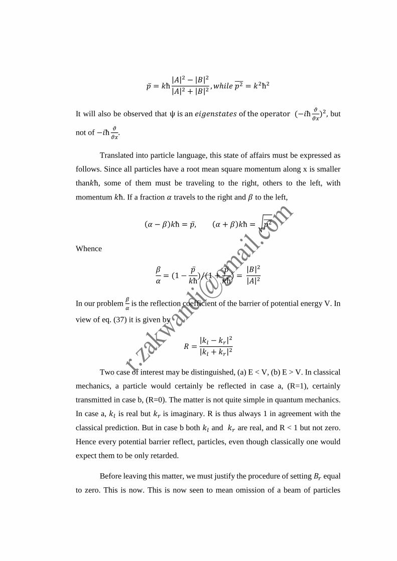
Let us take V to be the step function given by the solid line in Fig. 1, that is: 𝑉 =

0 𝑖𝑓 𝑥 < 0, 𝑉 = 𝑉 = 𝑐𝑜𝑛𝑠𝑡𝑎𝑛𝑡 𝑖𝑓 𝑥 > 0. The solutions for the two regions are

easily written down:

11 Another procedure is discussed for instance in Sommerfeld. A., “Atombau und Spektrallinien,”

Vol. II.

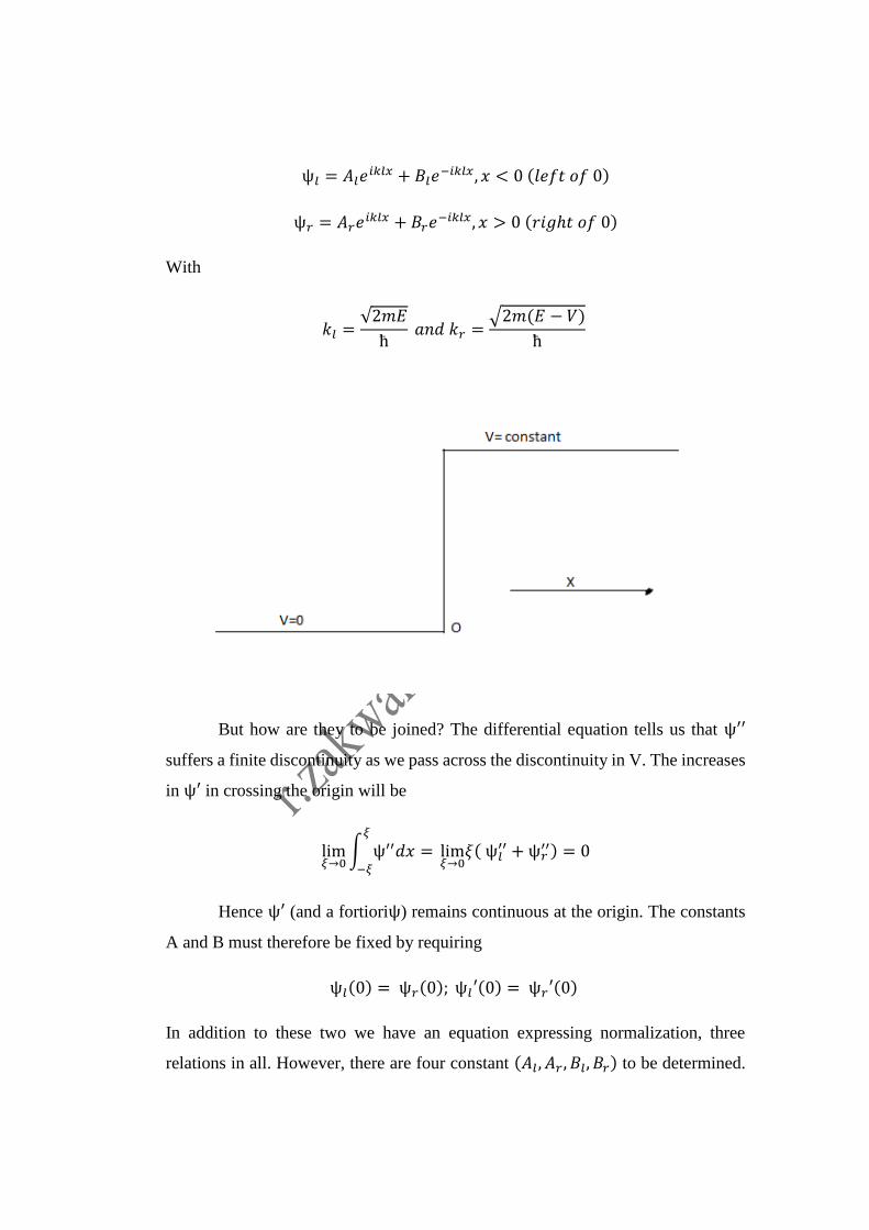
ψ𝑙 = 𝐴𝑙𝑒𝑖𝑘𝑙𝑥 + 𝐵𝑙𝑒

−𝑖𝑘𝑙𝑥, 𝑥 < 0 (𝑙𝑒𝑓𝑡 𝑜𝑓 0)

ψ𝑟 = 𝐴𝑟𝑒𝑖𝑘𝑙𝑥 + 𝐵𝑟𝑒

−𝑖𝑘𝑙𝑥, 𝑥 > 0 (𝑟𝑖𝑔ℎ𝑡 𝑜𝑓 0)

With

𝑘𝑙 =√2𝑚𝐸

ћ 𝑎𝑛𝑑 𝑘𝑟 =

√2𝑚(𝐸 − 𝑉)

ћ

But how are they to be joined? The differential equation tells us that ψ′′

suffers a finite discontinuity as we pass across the discontinuity in V. The increases

in ψ′ in crossing the origin will be

lim𝜉→0

∫ ψ′′𝑑𝑥 = 𝜉

−𝜉

lim𝜉→0

𝜉( ψ𝑙′′ + ψ𝑟

′′) = 0

Hence ψ′ (and a fortioriψ) remains continuous at the origin. The constants

A and B must therefore be fixed by requiring

ψ𝑙(0) = ψ𝑟(0); ψ𝑙′(0) = ψ𝑟′(0)

In addition to these two we have an equation expressing normalization, three

relations in all. However, there are four constant (𝐴𝑙 , 𝐴𝑟 , 𝐵𝑙, 𝐵𝑟) to be determined.

The mathematical situation is therefore such that one of them may be chosen at will.

Let us then put 𝐵𝑟 equal to zero. The physical meaning of this will at once be clear.

On applying the continuity conditions we have

A𝒍 + B𝑙 = 𝐴𝑟; 𝑘𝑙(A𝒍 − B𝑙) = 𝑘𝑟𝐴𝑟

Whence

Bl =𝑘𝑙 − 𝑘𝑟𝑘𝑙 + 𝑘𝑟

𝐴𝑙

The coefficient A and B have a simple significance. Let us analyze from our

fundamental point of view a state function of the formψ = 𝐴𝑒𝑖𝑘𝑙𝑥 + 𝐵𝑒−𝑖𝑘𝑙𝑥. In

view of the third postulate (eq. 14’) it represents a mean momentum

�� = −𝑖 ћ∫ψ ∗ ψ′dx

∫ψ ∗ ψdx

And a mean square momentum

𝑝2 = −ћ2∫ψ ∗ ψ′′dx

∫ψ ∗ ψdx

We have intentionally left the limits of integration indefinite. In evaluating

the integrals occuring here we assume that the range of integration is very much

larger than the wave length of the particles, 2𝜋/𝑘. The integral over the last two

terms of ψ ∗ ψ = A ∗ A + B ∗ B + AB ∗ 𝑒2𝑖𝑘𝑥 + 𝐴 ∗ 𝐵𝑒−2𝑖𝑘𝑥 will then vanish, and

∫ψ ∗ ψdx = (|𝐴|2 + |𝐵|2)𝑙

𝑙 being the range of integration. By the similar procedure,

∫ψ ∗ ψ′dx = ik(|𝐴|2 + |𝐵|2)𝑙 𝑎𝑛𝑑 ∫ψ ∗ ψ′′dx = −ik(|𝐴|2 + |𝐵|2)𝑙

Hence

�� = 𝑘ћ|𝐴|2 − |𝐵|2

|𝐴|2 + |𝐵|2, 𝑤ℎ𝑖𝑙𝑒 𝑝2 = 𝑘2ћ2

It will also be observed that ψ is an 𝑒𝑖𝑔𝑒𝑛𝑠𝑡𝑎𝑡𝑒𝑠 of the operator (−𝑖ћ𝜗

𝜗𝑥)2, but

not of −𝑖ћ𝜗

𝜗𝑥.

Translated into particle language, this state of affairs must be expressed as

follows. Since all particles have a root mean square momentum along x is smaller

than𝑘ћ, some of them must be traveling to the right, others to the left, with

momentum 𝑘ћ. If a fraction 𝛼 travels to the right and 𝛽 to the left,

(𝛼 − 𝛽)𝑘ћ = ��, (𝛼 + 𝛽)𝑘ћ = √𝑝2

Whence

𝛽

𝛼= (1 −

��

𝑘ћ)/(1 +

��

𝑘ћ) =

|𝐵|2

|𝐴|2

In our problem 𝛽

𝛼 is the reflection coefficient of the barrier of potential energy V. In

view of eq. (37) it is given by

𝑅 =|𝑘𝑙 − 𝑘𝑟|

2

|𝑘𝑙 + 𝑘𝑟|2

Two case of interest may be distinguished, (a) E < V, (b) E > V. In classical

mechanics, a particle would certainly be reflected in case a, (R=1), certainly

transmitted in case b, (R=0). The matter is not quite simple in quantum mechanics.

In case a, 𝑘𝑙 is real but 𝑘𝑟 is imaginary. R is thus always 1 in agreement with the

classical prediction. But in case b both 𝑘𝑙 and 𝑘𝑟 are real, and R < 1 but not zero.

Hence every potential barrier reflect, particles, even though classically one would

expect them to be only retarded.

Before leaving this matter, we must justify the procedure of setting 𝐵𝑟 equal

to zero. This is now. This is now seen to mean omission of a beam of particles

travelling to the left in the region to the right of the origin. Had such a beam been

included, the physical condition corresponding to ψ would have implied the

incidence of two beams of particls upon the origin, one from the left and one from

the right. In that case, 𝛽

𝛼 is not the reflection coefficient of the barrier. The ψ-

function we have chosen permits that interpretation, for it corresponds to one beam

incident from the left, one reflected and one transmitted beam.

Problem. Prove that �� is the same whether it is computed to the left or to the right

of the origin. [use condition (37)].

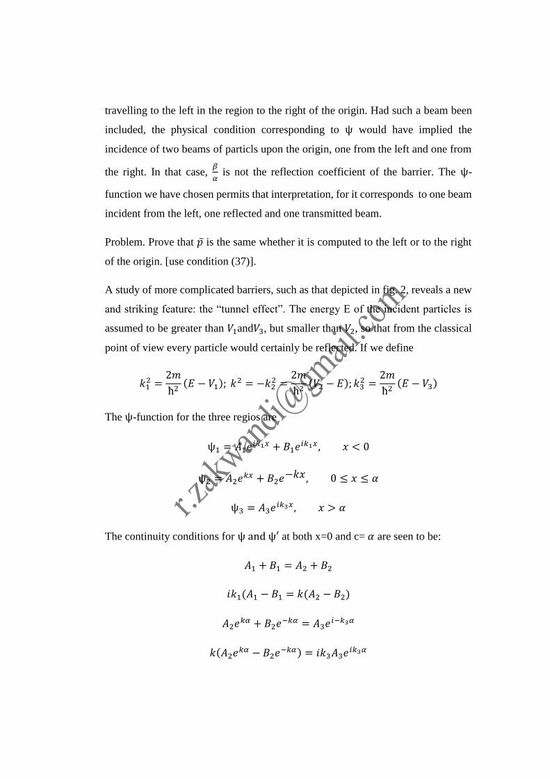
A study of more complicated barriers, such as that depicted in fig. 2, reveals a new

and striking feature: the “tunnel effect”. The energy E of the incident particles is

assumed to be greater than 𝑉1and𝑉3, but smaller than 𝑉2, so that from the classical

point of view every particle would certainly be reflected. If we define

𝑘12 =

2𝑚

ћ2(𝐸 − 𝑉1); 𝑘

2 = −𝑘22 =

2𝑚

ћ2(𝑉2 − 𝐸); 𝑘3

2 =2𝑚

ћ2(𝐸 − 𝑉3)

The ψ-function for the three regios are

ψ1 = 𝐴1𝑒𝑖𝑘1𝑥 + 𝐵1𝑒

𝑖𝑘1𝑥, 𝑥 < 0

ψ2 = 𝐴2𝑒𝑘𝑥 + 𝐵2𝑒

−𝑘𝑥, 0 ≤ 𝑥 ≤ 𝛼

ψ3 = 𝐴3𝑒𝑖𝑘3𝑥, 𝑥 > 𝛼

The continuity conditions for ψ and ψ′ at both x=0 and c= 𝛼 are seen to be:

𝐴1 + 𝐵1 = 𝐴2 + 𝐵2

𝑖𝑘1(𝐴1 − 𝐵1 = 𝑘(𝐴2 − 𝐵2)

𝐴2𝑒𝑘𝛼 + 𝐵2𝑒

−𝑘𝛼 = 𝐴3𝑒𝑖−𝑘3𝛼

𝑘(𝐴2𝑒𝑘𝛼 − 𝐵2𝑒

−𝑘𝛼) = 𝑖𝑘3𝐴3𝑒𝑖𝑘3𝛼

From these , 𝐵1, 𝐴2, and 𝐵2 may be eliminated. When this is done we obtain the

relation

𝐴1 =1

2𝐴3𝑒

𝑖𝑘3𝛼 {(1 +𝑘3𝑘1) cosh 𝑘𝛼 + 𝑖 (

𝑘

𝑘1−𝑘3𝑘) sinh 𝑘𝛼}

An argument similar to that which led us to identify the reflection coefficient R with

|𝐵|2/|𝐴|2, shows the transmissions coefficient of the present barrier to be

𝑇 =|𝐴3|

2𝑘3|𝐴1|2𝑘1

This may be computed from (38). In doing so we assume that 𝑘𝛼 ≫ 1 so that both

cosh 𝑘𝛼 and sinh 𝑘𝛼 become 1

2𝑒𝑘𝛼. Then

𝑇 = 16𝑘1𝑘3

(𝑘1 + 𝑘3)2 + (𝑘 −𝑘1𝑘3𝑘)2∙ 𝑒−2𝑘𝛼

As the width of the barrier increases, the factor 𝑒−2𝑘𝛼(sometimes called the

“transparency factor”) rapidly diminishes.

The surprising fact is that particles are able to “tunnel” through the barrier although

their kinetic energy is not great enough to allow them to pass it. Clasically speaking,

the kinetic energy of a particle would be

Negative while it is in region 2. Quantum mechanically, this statement is devoid of

meaning, since it is improper to compute 𝐸 − 𝑉 for this region alone.12

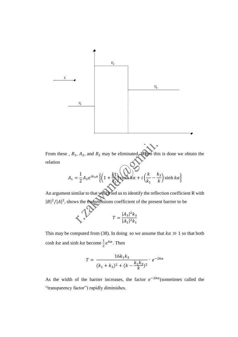
Fig. 3 gives a qualitative plot of the (real part of the) ψ-function in the three regions

here considered. It is seen that the barrier attenuates the wave coming from the left,

permitting a fraction of its amplitude to pass out at𝛼. The situation is quite

analogous t the passage of a wave through an absorbing layer.

11.11. Simple Harmonic Oscillator.-The potential energy, usually expressed in the

form 1

2𝑘𝑥2, is

1

2𝑚𝜔2𝑥2 when written in terms of the mass m and the classical

frequency 𝜔 = 2𝜋𝑣 of the oscillator. The meaning of 𝜔 is

12 More complicated barriers are discussed by Condon, E. U., Rev. Mod. Phys. 3, 43 (1931),

Eckart, C., Phys. Rev. 35, 1303 (1930)

Simply that of a parameter appearing in V; we must no longer expect the oscillator

to go back and forth 𝜔/2𝜋 times per second. The Schrὄdinger equation is

𝑑2𝜓

𝑑𝑥2+ (𝜖 − 𝛽2𝑥2)𝜓 = 0

If we use the abbreviations

𝜖 =2𝑚𝐸

ћ2, 𝛽 =

𝑚𝜔

ћ

The substitution 𝜉 = √𝛽𝑥 reduces (39) to the form of the differential equation for

“Hermit’s orthogonal functions”

𝑑2𝜓

𝑑𝜉2+ [1 − 𝜉2 + (

𝜖

𝛽− 1)]𝜓 = 0

Which was studied in chapter 2 (cf. Eq. 2-66). It was there found that its solution is

of the form 𝑒−𝜉2/2𝐻(𝜉),𝐻(𝜉) being solution of Hermite’s equation (2-62). Now

𝐻(𝜉) is a polynominal if the quantity𝛼, which corresponds to the present 1

2(𝜖

𝛽− 1),

as an integer. Unless this is true, H is a superposition of the infinite sequence (2-

63) and (2-64). But both of these approach infinity like𝑒𝜉2, as closer inspection will

show. If they are multiplied by𝑒−𝜉2/2, they will not yield a ψ-function which has

an integrable square between the limits −∞ 𝑎𝑛𝑑 +∞, which we are here assuming

to exist. Hence 𝐻(𝜉) must be chosen in its polynominal form, 𝐻𝑛(𝜉). Also,

1

2(𝜖/𝛽 − 1 ) = 𝑛, and this leads to

𝐸𝑛 = (𝑛 +1

2) ћ𝜔 = (𝑛 +

1

2) ℎ𝑣

𝜓𝑛 = 𝑐𝑒−(𝛽/2)𝑥2𝐻𝑛(√𝛽𝑥)

If theoscillator has three degrees of freedom, the Schrὄdinger equuation is

∇2𝜓 + (𝜖 − 𝛽2𝑟2)𝜓 = 0

When the same abbreviations as above are used. The method of separation of

variables (chapter 7) which involves the substitution of 𝑋(𝑥), 𝑌(𝑦), 𝑍(𝑧) for ψ at

once reduces this partial differential equation to three ordinary ones

𝑋′′ + (𝜖1 − 𝛽2𝑥2)𝑋 = 0, 𝑌′′ + (𝜖2 − 𝛽

2𝑥2)𝑌 = 0

𝑍′′ + (𝜖3 − 𝛽2𝑥2)𝑍 = 0

Provide that 𝜖1+𝜖2 + 𝜖3 = 𝜖. Each of these has a solution of the form (41), so that

𝜓𝑛1𝑛2𝑛3=𝑐𝑒

−(𝛽/2)𝑟2𝐻𝑛1(√𝛽𝑥)∙𝐻𝑛2(√𝛽𝑦)∙𝐻𝑛3(√𝛽𝑧)

𝐸𝑛1𝑛2𝑛2 = (𝑛1 + 𝑛2 + 𝑛3 +3

2)ћ𝜔

The orthogonality of the functions (41) has been proved in eq. 3-92. From this

formula, the normalizing constant c may also be computed. For if

∫ 𝑐2𝑒−𝛽𝑥2

∞

−∞

𝐻𝑛2(√𝛽𝑥)𝑑𝑥 = 𝛽−

12∫ 𝑐2𝑒−𝜉

2∞

−∞

𝐻𝑛2(𝜉)𝑑𝜉

= 𝑐2 ∙ 2𝑛𝑛!√𝜋

𝛽= 1

Then

𝑐 = (𝛽

𝜋)1/4

(𝑛! 2𝑛)−1/2

A similar computation, which involves three integrations, yields for the constant c

of eq. (42) the value

(𝛽

𝜋)1/4

(𝑛1! 𝑛2! 𝑛3! 2𝑛1+𝑛2+𝑛3)−1/2

Further mathematical details concerning the functions here encountered, as well as

table of the 𝐻𝑛-polynomials, are given in sec. 3.10.

Problem. The treatment above implide that the 3- dimensional oscillator was

istropic ; bound with equal force in all directions. Calculate eigenvalues and

eigenfunctions for an anisotropic oscillator with potential energy

𝑉 =1

2𝑚(𝜔1

2𝑥2 + 𝜔22𝑥2 + 𝜔3

2𝑥2)

11.12. Rigid Rotator, Eigenvalues Eigenfunctions of 𝐿2 . –A rigid rotator is a pair

of point masses held together by a rigid, inflexible and inextensible (massless)

bond. A diatomic molecule is a fiar approximation to a rigid rotator. Before

attempting to solve the Schrὄdinger equation for such a system it is well to digress

briefly and considen the eigenvalue equation for an operator which so far we have

not introduced, but which is easily constructed. We have seen that the operators

corresponding to the components of angular momentum of a particle are

𝐿𝑥 = −𝑖ћ (𝑦𝜕

𝜕𝑧− 𝑧

𝜕

𝜕𝑧)

𝐿𝑦 = −𝑖ћ (𝑧𝜕

𝜕𝑥− 𝑥

𝜕

𝜕𝑧)

𝐿𝑧 = −𝑖ћ (𝑥𝜕

𝜕𝑦− 𝑦

𝜕

𝜕𝑥)

From these, we wish to construct the operator

𝐿2 = 𝐿𝑥2 + 𝐿𝑦

2 + 𝐿𝑧2

It is advantageous to do this in polar (spherical) coordinates*13 putting 𝑥 =

𝑟 sin 𝜃 cos𝜑, 𝑦 = 𝑟 sin 𝜃 sin𝜑 𝑧 = 𝑟 cos 𝜃, 𝑤𝑒 ℎ𝑎𝑣𝑒

𝜕

𝜕𝑥= 𝑠𝑖𝑛𝜃𝑐𝑜𝑠𝜑

𝜕

𝜕𝑟+1

𝑟𝑐𝑜𝑠𝜃𝑐𝑜𝑠𝜑

𝜕

𝜕𝜃−1

𝑟

𝑠𝑖𝑛𝜑

𝑠𝑖𝑛𝜃

𝜕

𝜕𝜑

𝜕

𝜕𝑦= 𝑠𝑖𝑛𝜃𝑠𝑖𝑛𝜑

𝜕

𝜕𝑟+1

𝑟𝑐𝑜𝑠𝜃𝑠𝑖𝑛𝜑

𝜕

𝜕𝜃+1

𝑟

𝑐𝑜𝑠𝜑

𝑠𝑖𝑛𝜃

𝜕

𝜕𝜑

𝜕

𝜕𝑧= 𝑐𝑜𝑠𝜑

𝜕

𝜕𝑟−1

𝑟𝑠𝑖𝑛𝜃

𝜕

𝜕𝜃

When these results are introduced in (44) and (45) is formed, there results

𝐿2 = −ћ2 {1

sin 𝜃

𝜕

𝜕𝜃(sin 𝜃

𝜕

𝜕𝜃) +

1

𝑠𝑖𝑛2𝜃

𝜕2

𝜕𝜑2}

The observable value which the square of the angular momentum may assume are

the eigenvalues p of the equation

𝐿2𝜓 = 𝑝𝜓

This equatioan is easily solved by the metode of separation of variables (ef. Chapter

7 ). Clearly, ψ is a function of 𝜃 and 𝜑. Put ψ = Ө (𝜃) . 𝛷(𝜑) into (47). This equation

will then break up into two ordinary equations (the process is analogous to the

constructions of eqs. 7-42a and 7-42b):

ћ2 {1

sin 𝜃

𝜕

𝜕𝜃(sin 𝜃Ө′) −

𝑚2

𝑠𝑖𝑛2𝜃Ө +

𝑝

ћ2Ө} = 0

𝛷′′ = −𝑚2𝛷

13 See also the problem at the end of this section

This equation therefore has the solution 𝛷= const.𝑒𝑖𝑚𝜑, m an integar. The equation

for associated Legendre functions, (eq. 7.45b), except that the constant 𝑙(𝑙 + 1)

appearing there is here replaced by𝑝/ћ2. The solution previously obtained is

Ө = 𝑠𝑖𝑛𝑚𝜃𝑑𝑚

𝑑(𝑐𝑜𝑠𝜃)𝑚𝑃𝑙(cos 𝜃)

Now the legendre function 𝑃𝑙 was shown to behave singulary at cos 𝜃 = ±1 unless

𝑙 is an integer, in fact it would countain unlimited powers of 𝑥(= cos 𝜃). The same

would be true for Ө if 𝑙 were arbitrary. But in that case∫ψ ∗ ψdr, which contains

the factor

∫ Ө2 sin 𝜃𝑑𝜃 = ∫ Ө2𝑑𝑥1

−1

𝜋

0

Would centainly not exist. We conclude, therefore, that 𝑙 must be an integar, and

that the eigenfunction of 𝐿2 are

𝑝 = 𝑙(𝑙 + 1)ћ2

On other hand, the eigenfunctions of 𝐿2 are of the form

𝑠𝑖𝑛𝑚𝜃𝑑𝑚

𝑑𝜃𝑚𝑃𝑙(𝑐𝑜𝑠𝜃)𝑒

𝑖𝑚𝜑 = 𝑃𝑙𝑚(cos 𝜃) 𝑒𝑖𝑚𝜑

In the notation adopted in chapter 3 (ef. Eq. 3-43). Since the eigenvalue 𝑝 does not

depend on 𝑚 but only on, functions like (48) with different 𝑚 will satisfy eq. (47)

. The most general solution of that equation is therefore, 14

14 We define here and elsewhere: 𝑃𝑙

−𝑚 = 𝑃𝑙𝑚, 𝑎𝑠 𝑖𝑛 (3 − 62)

𝜓 = ∑ 𝑐𝑚𝑃𝑙𝑚(cos 𝜃)𝑒𝑖𝑚𝜑

𝑙

𝑚−−𝑙

In chapter 7 this function has already been encountered; it is called a spherical

harmonic and denoted by 𝑌𝑙(𝜃, 𝜑) (ef. Eq. 7-43 et seq.). Hence

ψ = 𝑌𝑙(𝜃, 𝜑)

Since 𝑑𝑟 = sin 𝜃𝑑𝜃𝑑𝜑, normalization requires that

∫ 𝑑𝜑𝜓 ∗ 𝜓 = 1𝜋

0

Whan (49) is inserted the integral becomes

2𝜋∑𝑐𝑚 ∗ 𝑐𝑚∫ [𝑃𝑙𝑚(𝑥)]2𝑑𝑥

1

−1

=4𝜋

2𝑙 + 1∑|𝑐𝑚|

2(𝑙 + 𝑚)!

(𝑙 − 𝑚)!

𝑙

−𝑙

𝑙

−𝑙

(cf. Eq. 3-62). Hence, for normalization, the constants 𝑐𝑚 appearing in (49) must

satisfy the relation

∑ |𝑐𝑚|2

𝑙

𝑚=−𝑙

(𝑙 + 𝑚)!

(𝑙 − 𝑚)!=2𝑙 + 1

4𝜋

And are otherwise arbitrary.

We are now ready to return to the problem of the rigid rotator. In the first place we

shall assume it proper to replace it by a single mass, rigidly tied to center of rotation,

and having the same moment of inertia as the original system. The condination upon

the state function in accord with this assumption-aside simple 𝑟 = 𝑎,a constant. The

best procedure is therefore to write down the SchrÖdinger equation for a particle

moving in three dimensions, and then to put 𝑟 = 𝑎, 𝑑 ψ /dr = 0. This requares the

use of polar (spherical) coordinates. The potential energy, in this case, is cleary

constant and may be taken to be zero.

SchrÖdinger’s equation reads15 (ef. Chapter 5 for transformation of ∇2)

1

𝑟2𝜕

𝜕𝑟(𝑟2

𝜕𝜓

𝜕𝑟) +

1

𝑟2 sin 𝜃

𝜕

𝜕𝜃(sin 𝜃

𝜕𝜓

𝜕𝜃) +

1

𝑟2𝑠𝑖𝑛2𝜃

𝜕2𝜓

𝜕𝜑2+2𝑀

ћ2𝐸𝜓 = 0

When 𝑟 is put equal to a the first term on the left vanisehes, and the remainder

becomes very similar to𝐿2𝜓. Indeed if we introduce, a new operator ⋀2 definde

as(1/ћ2)𝐿2, eq. (51) may be written

⋀2𝜓 =2𝑀𝑎2

ћ2𝐸𝜓

But the eigenvalues of a ⋀2 are obviously𝑙(𝑙 + 1), and its eigenfunctions are the

same as those of 𝐿2. The constant(2𝑀𝑎2/ћ2)𝐸, must be identified with𝑙(𝑙 + 1).

Hence the eigenvalues and eigenfunctions are

𝐸 =ћ2

2𝑀𝑎2𝑙(𝑙 + 1); 𝜓𝑙,𝑚 = 𝑌1(𝜃, 𝜑)

Problem. Show by vector algebra that

−⋀2 = (𝑟 𝑥 ∇)2 = −𝑟2∇2 + 2𝑟𝜕

𝜕𝑟+ 𝑟2

𝜕2

𝜕𝑟2

Hint: Note that(𝑟 𝑥 ∇)2 = 𝑟 ∙ [∇ 𝑥 (𝑟 𝑥 ∇)]. Then use (4-26) for∇ 𝑥 𝑈 𝑥 𝑉.

11.13. Motion in a Central Field. –By central field is meant a field of force in which

the potential energy is a function of r only; V is independent of 𝜃 and 𝜑. The

isotropic three-dimentional oscillator treated in sec. 11 is an example of motion in

a central field. Another is the motion of a particle in a coulomb field. It is to this

last example, an electron attracted by a positive point charge (hydrogen atom), that

we shall chiefly direct our attention. But before considering this spesific case a few

general features of the central field problem will be exposed.

15 To avoid confusion, we write M for the electron mass in this section, returning to the symbol m

in the next.

It is now clear that the Laplacian, ∇2, in spherical polar coordinates has the form.

∇2=1

𝑟2{𝜕

𝜕𝑟(𝑟2

𝜕

𝜕𝑟) + ⋀2}

Where ⋀2 is given by (by) divided by −ћ2. The eigenvalues of the ⋀2 are 𝑙(𝑙 + 1).

The Schrὄdinger equation therefore reads

1

𝑟2{𝜕

𝜕𝑟(𝑟2

𝜕𝜓

𝜕𝑟) − ⋀2𝜓} +

2𝑚

ћ2[𝐸 − 𝑉(𝑟)]𝜓 = 0

We write 𝜓 as a product of a function R(r) and another.𝐴(𝜃, 𝜑), which depends

only on the angles. The operator ⋀2 acts only on A. Eq. (55), after multiplication

by 𝑟2 and subsequent division by𝑅 ∙ 𝐴, has the form

𝑑𝑑𝑟(𝑟2

𝑑𝑅𝑑𝑟)

𝑅+2𝑚𝑟2

ћ2[𝐸 − 𝑉(𝑟)] =

⋀2𝐴

𝐴

The left-hand side of this equation is a function of 𝑟 alone, the right a function of

𝜃and𝜑. By the argument which is familiar from chapter 7, each side must be a

constant, say𝑎. Thus

⋀2𝐴 = 𝑎𝐴

But this is simply the eigenvalue equation for⋀2. We see, then, that

𝑎 = 𝑙(𝑙 + 1), 𝑎𝑛𝑑 𝐴 = 𝑌1(𝜃, 𝜑)

The left-hand side of (56) becomes

𝑑

𝑑𝑟[𝑟2

𝑑𝑅

𝑑] +

2𝑚𝑟2

ћ2[𝐸 − 𝑉(𝑟) −

𝑙(𝑙 + 1)

2𝑚𝑟2ћ2] 𝑅 = 0

And the substitution 𝑈(𝑟) = 𝑟𝑅(𝑟) reduce this to

𝑈′′ +2𝑚

ћ2[𝐸 − 𝑉(𝑟) −

𝑙(𝑙 + 1)ћ2

2𝑚𝑟2]𝑈 = 0

The depelovement so far has been totally independent of the form of V, except in

assuming it to be a function of 𝑟 alone. The result obtained are therefore valid for

any central field. Summarizing them, we may say:

The energy states of a particle in a central field are always of the form

𝜓 =1

𝑟𝑈𝑙(𝑟)𝑌𝑙(𝜃, 𝜑)

And the function 𝑈𝑙 is determined by eq. (57b). It was necessary to add a subscript

𝑙 𝑡𝑜 𝑈 because the differential equation contains 𝑙 as a parameter. The energies E

are obtained solely from eq. (57b)

That equation looks very much like the one-dimensional Schrὄdinger equation,

𝜓′′ +2𝑚

ћ2[𝐸 − 𝑉(𝑥)]𝜓 = 0

But with the term 𝑙(𝑙 + 1)ћ2/2𝑚𝑟2 added to the normal potential

energy. What is the meaning of that term? In classical mechanics, the energy of a

particle moving in three dimensions differs from that of a one-dimensional particle

by the kinetic energy of a rotation1

2𝑚𝑟2𝜔2. This is precisely the quantity𝑙(𝑙 +

1)ћ2/2𝑚𝑟2, for we have seen that 𝑙(𝑙 + 1)ћ2 is the certain value of the square of

the angular momentum for the state𝑌𝑙, in classical language(𝑚𝑟2𝜔)2, which when

divided by2𝑚𝑟2, gives exactly the kinetic energy of rotation.

There is, however, one further difference between (57b) and (58). The

fundamental range of 𝑟 in (57b) starts at 𝑟 = 0 and is limited to positive values,

whereas the range of 𝑥 in (58) may include negative values. This fact often has a

more important effect on the eigenvalues than the addition of the terms just

mentioned.

Let us now solve eq. (57b), assuming a Coulomb field, e.g., 𝑉(𝑟) = −𝑒2/𝑟.

The energies E will then be the energy levels of the hydrogen atom16. For

sufficiently large 𝑟 the solution is determined by

𝑈′′ − (𝛼

2)2

𝑈 = 0

Provided we define

(𝛼

2)2

= −2𝑚𝐸

ћ2

The solution of (59) is𝑈∞ = 𝑐1𝑒(𝛼/2)𝑟 + 𝑐2𝑒

(𝛼/2)𝑟, and this represents the behavior

of the correct𝑈 𝑎𝑡 ∞. Let us first suppose that 𝛼 is real, which means that the energy

of the particle is negative. U will then certainly not have an integrable square (note

that the radial integral has then the form ∫ 𝑅2𝑟2𝑑𝑟 = ∫𝑈2𝑑𝑟∞

0 if the coefficient 𝑐1

fails to vanish. But we cannot simply put it equal to zero because we have boundary

conditions to full fill! Without going further in our analysis at the moment we

expect, therefore, that only special values of 𝛼 will produce accetable solutions

when 𝛼 is real. If the total energy of the particle is negative (classically speaking,

the particle is bound to the attracting center), the energy is expected to be quantized.

The following analysis will bear this out.

If 𝛼 is imaginary, which means that E is positive, 𝑈∞ shows sinusoidal behaviot. It

has, in fact, the typical form of the state function for a free particle, and the failure

of normalization occurs in the milder manner which we have previously found

associated with the presence of a continuous spectrum of eigenvalues. There is

indeed no way of choosing 𝑐1 𝑜𝑟 𝑐2

Or 𝛼 which would make one 𝑈∞ more acceptable than another. We conclude that,

when E is positive, the energy spectrum is continuous.

16 If 𝑒2 is replaced by 𝑍𝑒2, 𝑍 = 2 represents ionized helium, Z=3 doubly ionized lithium, etc.

From the point of view of classical physics this result is welcome, for when E is

positive the particle is ionized and moves through the space, its energy being

unrestricted.

We now discuss the bound states in a more rigorous manner. Put𝐸 = −𝑊, so that

𝑊 is positive. Our interest will now return to eq. (57a) which forms a more suitable

basis for the present discussion. Let𝑟 = 𝑥/𝛼, where 𝛼 is defined by (60). Eq. (57a)

then reads, after some cancellation,

𝑥𝑑2𝑅

𝑑𝑥2+ 2

𝑑𝑅

𝑑𝑥+ [2𝑚𝑒2

ћ2𝛼−𝑥

4−𝑙(𝑙 + 1)

𝑥] 𝑅 = 0

But this is precisely the differential equation for associated Laguere functions,

which was studied in chapter 2 (cf.eq.71). for our immadiatepurpose we shall write

that equation with n* in place of n, since otherwise our nation would be in conflict

with physical convention. To summarize the result of sec. 2.16:

The equation

𝑥𝑦′′ + 2𝑦′ + [𝑛 ∗ −𝑘 − 1

2−𝑥

4−𝑘2 − 1

4𝑥] 𝑦 = 0

Has solution possessing an integrable square17 of the form

𝑦 = 𝑒−𝑥/2𝑥(𝑘−1)/2𝐿𝑛∗𝑘 (𝑥)

Provided n* and k are positive integers. Moreover, 𝑛 ∗ −𝑘 ≥ 0 sinc otherwise 𝐿𝑛∗𝑘

would vanish.

On comparing (61) and (62) we find, in the first place, that(𝑘2 − 1)/4 = 𝑖(𝑙 + 1),

hence

𝑘 = 2𝑙 + 1

Secondly,

17 The reader should convince himself of this fact by going back to see sec. 2.16.

𝑛 ∗ −𝑘 − 1

2= 𝑛 ∗ −𝑙 =

2𝑚𝑒2

ћ2𝛼

When the value of 𝛼 is inserted here and the relation is solved for W, we find

𝑊 =1

2

𝑚𝑒4

(𝑛 ∗ −𝑙)2ћ2

Because of the conditions on n* and k, the quantity 𝑛 ∗ −𝑙 cannot be zero. It is

usually denoted by n and called the total quantm number (after the role it played in

the Bohr theory). Our conclusion, then, is this: The energy states of the hydrogen

atom are

𝑊𝑛 = −𝐸𝑛 =1

2 2𝑚𝑒2

𝑛2ћ2

And the corresponding eigenfnctions are, in accordance with (63),

𝑅𝑛,𝑙 = 𝑐𝑛,𝑙𝑒−𝑥2𝑥𝑙𝐿𝑛+𝑙

2𝑙+1(𝑥)

The variable x being defined by

𝑥 = 𝛼𝑟 =√8𝑚𝑊

ћ𝑟 =

2𝑚𝑒2

𝑛ћ2𝑟

In the Bohr theory of hydrogen, the first orbit has a radius

𝑎0 =ћ2

𝑚𝑒2= 0,53 𝑥 10−8 𝑐𝑚

It sometimes convient to express x in terms of it. Thus𝛼 = 2/𝑛𝑎0, and

𝑥 =2

𝑛 𝑟

𝑎0

It is to be noticed that x represents a different variable for each energy state; the

quantum number n determining W appears as a scale factor in the dimensionless

variable x.

Some integrals involving𝑅𝑛,𝑙, which occur frequently in physical and chemical

problem, have been evaluated in sec. 3.11., see also the example at the end of sec.

3.11, which is of interest in this connection.

For later use, we write down in explicit form the state function for the normal

hydrogen atom. It is

𝑅1,0 = 𝑐1,0𝑒−𝑟/𝑎0𝐿1

1 = 2𝑎0−3/2𝑒−𝑟/𝑎0

For this state 𝑌1 = 𝑐𝑜𝑛𝑠𝑡𝑎𝑛𝑡 = (4𝜋)−1/2 when the function is normalized. Hence

the total ground state function is

𝜓0 = (𝜋𝑎03)−1/2𝑒−𝑟/𝑎0

Ψ-functions for the higher states are listed in explicit form in Pauling and Wilson18.

When the charge on the nucleus is not e but𝑍𝑒, 𝑎0 must be replaced by𝑎0/𝑍, so that

𝜓0 = (𝑍3

𝜋𝑎03)

1/2

𝑒−𝑍𝑟/𝑎0

Problem a., using the result of chapter 3, show that the normalizing factor in (65)

is

𝑐𝑛,𝑙 = (2

𝑛𝑎0)3/2

{(𝑛 − 𝑙 − 1)!

2𝑛[(𝑛 + 𝑙)!]3}

1/2

Problem b. Work out the problem of the isotropic oscillator using spherical

coordinates, and show that the result agree with those obtained in (42) and (43).

11.14 Symmetrical Top. –In dealing with the problem f the rotating rigid body

attention must be given to the kinetic energy operator. To obtain it we first observe

18 Pauling, L., and Wilson, E. B., Jr., “Introduction to Quantum Mechanics” McGraw-Hill Book

Co., 1935.

that its form in rectangular coordinates, for the n particle problem (cf. Sec. 11.31)

is 𝑇𝜓 = − ћ2

2∑

∇𝑖2

𝑚𝑖𝜓𝑛

𝑖−1

The position of a rigid body is best expressed in terms of the Eulerian angles,

introduced in sec. 9.5. it was there shown that the classical kinetic energy is given

by

𝑇𝑐 =1

2∑𝑚𝑖(𝑥𝑖

2 + 𝑦𝑖2 + 𝑧𝑖

2)

𝑛

𝑖=1

=1

2𝐴𝛽2 +

1

2𝐴𝛼2𝑠𝑖𝑛2𝛽 +

1

2𝐶(𝛾 + 𝛼 cos 𝛽)2

Let us define a line element constructed from the Cartesian coordinates

𝜉𝑖 = √𝑚𝑖𝑥𝑖 , ƞ𝑖 = √𝑚𝑖𝑦𝑖 , 𝜁𝑖 = √𝑚𝑖𝑧𝑖

As follows:

𝑑𝑠2 =∑(𝑑

𝑛

𝑖=1

𝜉𝑖2 + 𝑑ƞ𝑖

2 + 𝑑𝜁𝑖2)

This is clearly identical with2𝑇𝑐𝑑𝑡2. From the form of 𝑇𝑐 in Eulerian coordinates it

is seen that 𝑑𝑠2 in these coordinates is given by

𝑑𝑠2 = 𝐴𝑑𝛽2 + 𝐴 𝑠𝑖𝑛2𝛽𝑑𝛼2 + 𝐶(𝑑𝛾 + cos 𝛽𝑑𝛼)2

Now the quantum mechanical form of T is the Laplacian operator corresponding to

the line element𝑑𝑠2, multiplied by −ћ2/2. The problem is therefore to transform

the Laplacian operator from a set of coordinates in terms of which the line element

is given by (68), to a new set in terms of which the lines element is (69). This

problem has been discussed in sec. 5.17. if

𝑑𝑠2 =∑𝑔𝜆,𝜇𝑑𝑞𝜆𝑑𝑞𝜇𝜆,𝜇

Then

∇𝑞2𝜓 =

1

√𝑔∑

𝜕

𝜕𝑞𝜆[√𝑔 𝑔𝜆,𝜇

𝜕

𝜕𝑞𝜆𝜓]

𝜆,𝜇

On indentifying the 𝑔𝜆,𝜇 from (69) we find (putting 𝑞1 = 𝛽, 𝑞2 = 𝛼, 𝑞3 = 𝛾)

(𝑔𝜆,𝜇) = (

𝐴 0 00 𝐴𝑠𝑖𝑛2𝛽 + 𝐶𝑐𝑜𝑠2𝛽 𝐶 cos 𝛽0 𝐶 cos 𝛽 𝐶

)

And hence

(𝑔𝜆,𝜇) =

(

1

𝐴0 0

01

𝐴𝑠𝑖𝑛2𝛽−

cos𝛽

𝐴𝑠𝑖𝑛2𝛽

0 −cos 𝛽

𝐴𝑠𝑖𝑛2𝛽

1

𝐶+𝑐𝑜𝑠2𝛽

𝐴𝑠𝑖𝑛2𝛽)

, 𝑔 = 𝐴2𝐶 𝑠𝑖𝑛2𝛽

When these results are substitued in the expression for ∇𝑞2𝜓 we have

𝑇𝜓 = −ћ2

2∇𝑞2= −

ћ2

2 sin 𝛽{𝜕𝜓

𝜕𝛽(𝑠𝑖𝑛𝛽

𝐴

𝜕𝜓

𝜕𝛽) +

𝜕

𝜕𝛼[𝑠𝑖𝑛𝛽

𝐴𝑠𝑖𝑛2𝛽

𝜕𝜓

𝜕𝛼−𝑠𝑖𝑛𝛽𝑐𝑜𝑠𝛽

𝐴𝑠𝑖𝑛2𝛽

𝜕𝜓

𝜕𝛾]

+𝜕

𝜕𝛾[−𝑠𝑖𝑛𝛽𝑐𝑜𝑠𝛽

𝐴𝑠𝑖𝑛2𝛽

𝜕𝜓

𝜕𝛼+ (

𝑠𝑖𝑛𝛽

𝐶+𝑠𝑖𝑛𝛽𝑐𝑜𝑠2𝛽

𝐴 𝑠𝑖𝑛2𝛽)𝜕𝜓

𝜕𝛾]}

= −ћ2

2𝐴{𝜕2𝜓

𝜕𝛽2+ cot 𝛽

𝜕𝜓

𝜕𝛽+

1

𝑠𝑖𝑛2𝛽

𝜕2𝜓

𝜕𝛼2+ (𝑐𝑜𝑡2𝛽 +

𝐴

𝐶)𝜕2𝜓

𝜕𝛾2

−2 cos 𝛽

𝑠𝑖𝑛2𝛽

𝜕2𝜓

𝜕𝛼𝜕𝛾}

Since the potential energy in this problem is zero, the Schrὄdinger equation

becomes

𝑇𝜓 = 𝐸𝜓

It is separable; for if we put

𝜓 = 𝑢(𝛼) ∙ 𝑣(𝛾) ∙ 𝑤(𝛽)

The function 𝑢 𝑎𝑛𝑑 𝑣 are seen to satisfy equations of the form

𝑎2𝑑2𝑢

𝑑𝛼2+ 𝑎1

𝑑𝑢

𝑑𝛼+ 𝑎0𝑢 = 0, 𝑏2

𝑑2𝑢

𝑑𝛾2+ 𝑏1

𝑑𝑢

𝑑𝛾+ 𝑏0𝑢 = 0

Where the coefficient 𝑎0, 𝑎1, 𝑎2 are not function of𝛼, and the coefficients 𝑏0, 𝑏1, 𝑏2

are not function of 𝛾. Such equations have solutions

𝑢 = 𝑒𝑖𝑚𝛼, 𝑣 = 𝑒𝑖𝑘𝛾

m and k being roots of algebraic quadratic equations involving the coefficients

𝑎 𝑎𝑛𝑑 𝑏. However, these need not be solved here, since the condition of single-

valuedness dictates that m and k be integers. We therefore put

𝑢 = 𝑒𝑖𝑀𝛼, 𝑣 = 𝑒𝑖𝐾𝛾

𝑀,𝐾 = 0, ±1, ±2, 𝑒𝑡𝑐

The Schrὄdinger equation now reduces to the following ordinary differential

equation in the independent variable𝛽:

𝑤′′ + cot 𝛽𝑤′

−[𝑀2

𝑠𝑖𝑛2𝛽+ (𝑐𝑜𝑡 2𝛽 +

𝐴

𝐶)𝐾2 − 2

cos𝛽

𝑠𝑖𝑛2𝛽𝐾𝑀 −

2𝐴

ћ2𝐸]𝑤 = 0

The substutions

1

2(1 − 𝑐𝑜𝑠𝛽) = 𝑥

𝑤(𝛽) = 𝑥|𝐾−𝑀|2 (1 − 𝑥)

|𝐾+𝑀|2 𝐹(𝑥)

Which are suggested when this equation is examined for its singularities along the

lines of chapter 2, transform it to

(𝑥2 − 𝑥)𝑑2𝐹

𝑑𝑥2+ [(1 + 𝑝)𝑥 − 𝑞]

𝑑𝐹

𝑑𝑥− 𝑛(𝑝 + 𝑛)𝐹 = 0

The new parameters being defined as follows:

𝑝 = 1 + |𝐾 −𝑀| + |𝐾 +𝑀|

𝑞 = 1 + |𝐾 −𝑀|

𝑛(𝑝 + 𝑛) = 𝐴(2𝐸

ћ2−𝐾2

𝐶) + 𝐾2 −

1

4(𝑝 − 1)2 −

1

2(𝑝 − 1)

This last relation, when rearranged, may be written

𝐸 =ћ2

2𝐴[(𝑛 +

𝑝 + 1

2) (𝑛 +

𝑝 − 1

2) + (

𝐴

𝐶− 1)𝐾2]

Reference to chapter to chapter 2, eq. 56 will show at once that the differential

equation for F is none other than the familiar hypergeometric equation defining the

Jacobi polynomials, provided n is an integer. Unless this condition is satisfied, F

will diverge for𝑥 = 1, i.e., for𝛽 = 𝜋.

Eq. (70) takes a simpler form when we introduce the new quantum number

𝐽 = 𝑛 +𝑝 − 1

2= 𝑛 +

1

2|𝐾 −𝑀| +

1

2|𝐾 +𝑀|

Which is evidently a positive integer or zero. We then obtain

𝐸 =ћ2

2𝐴[𝐽(𝐽 + 1) + (

𝐴

𝐶− 1)𝐾2]

An equation which determines the energy levels of the symmetrical top. Note that

the quantity 1

2|𝐾 − 𝑀| +

1

2|𝐾 + 𝑀| is equal to the larger of the two integers K and

M; in consequence of this neither |𝐾| nor |𝑀| can be greater than J.

The energy levels of the spherical top (A=C) are those already obtained in sec. 11.12

(cf. Eq. 11-53).

MATRIX MECHANICS

11.15 General Remarks and procedure. –The formulation of quantum mechanics

we have given in the foregoing sections was historically precede by Heisenberg’s

matrix theory. The latter, while it appears at first glance to be an altogether different

mathematical structure, strikingly produced the same result as the former. But when

the initial amazement subsided both formulations were recognized as equivalent. In

the present text the Schrὄdinger -Dirac theory was discussed first because its axioms

seem perhaps less strange, and because its point of view has been more widely

adopted. The terminology of matrix mechanics, however, enjoys great popularity

and its often conducive to clarity of expression.

Its possible, and perhaps pedagogically worthwhile, to derive Heisenberg’s theory

from the postulates of part of this chapter. But when this is done, the impressive

element of uniqueness which attaches to matrix mechanics is completly lost. To

preserve it we proceed to state the basic facts of the theory first, to give an example

of its application, and then to exhibit its relation to the preceding developments. We

can afford to be brief, for when the equivalence of the theories is once established,

no new insight is likely to be gained by deducing former result over again in a

different manner. As before, attention will be limited to what we have called

quantum statics. The principal facts of chapter 10 will be used.

Heisenberg associates with every observable a square Hermitian matrix. As in the

Schrὄdinger theory, one of the chief concerns of matrix mechanics is the

determination of the measureable values of an observable. Let it be desired to find

the observable values of a quantity H, which, classically, is a function of the

cartesian coordinates 𝑞𝑖 and momenta𝑝𝑖,𝐻 = 𝐻(𝑞𝑖. . . 𝑞𝑛; 𝑝𝑖. . . 𝑝𝑛) in our

example we shall specify H to be the energy, but this restriction is not necessary.

Heisenberg’s directions are the find a set of matrices𝑸𝟏, 𝑸𝟐, ..., 𝑸𝒏; 𝑷𝟏, 𝑷𝟐, … , 𝑷𝒏

which (a) satisfy the commutation rules

𝑸𝒎𝑸𝒏 − 𝑸𝒏𝑸𝒏 = 𝑶; 𝑷𝒎𝑷𝒏 − 𝑷𝒏𝑷𝒎 = 𝑶; 𝑷𝒎𝑸𝒏 − 𝑸𝒏𝑷𝒎 = −𝒊ℏ𝜹𝒏𝒎𝑬

(11–71)

where E is the unit matrix; (b) render the matrix

H (𝑸𝟏, …𝑸𝒏; 𝑷𝟏… 𝑷𝒏) diagonal (11–72)

By H (𝑸𝟏… 𝑸𝒏; 𝑷𝟏… 𝑷𝒏) is meant, of course, the matrix which is the

same funcition of matrices 𝑸𝟏… 𝑷𝒏 that the ordinary function H is of 𝑞1… 𝑝𝑛.

The existence of the matrix H and its uniqueness will be assumed. when such a set

of matrices has been found, the diagonal elements of H will be the measurable

values in question. (It is also true that the squares of the absolute values of the

elements (𝑄𝑖)𝜆𝜇 are simply related to spectroscopic transition probabilities, as will

be show later; but this does not concern us here). We illustrate the power of the

method by an example.

11.16. Simple Harmonic Oscillator.

The Hamiltonian function is (cf. sec. 11)

H = 𝑝2

2𝑚 +

1

2𝓂𝜔2𝑞2

Hence, if P and 𝑸 are matrices,

𝑯 = (𝑸,𝑷) = 1

2𝑚 (𝑷𝟐 + 𝑚2𝜔𝟐𝑸2)

The straightforward way of working this problem would be to select a set

of matrices such as, e.g.,

𝑄𝜆𝜇 = 𝛿𝜇,𝜆−1, 𝑃𝜆𝜇 = −𝑖ℏ𝜇𝛿𝜇,𝜆+1 (11-73)

which satisfy the commutation rule (71)

(𝑃𝑄)𝜆𝜇 (𝑄𝑃)𝜆𝜇 = −𝑖ℏ𝜇𝛿𝜆𝜇 (11-71a)

as the reader may verify. These – must then be subjected to a similarity

transformation with some other matrix, say S, until the new matrices

𝑸′ = 𝑺−𝟏 𝑸𝑺,𝑷′ = 𝑺−𝟏𝑷𝑺

when substituted in H, make H a diagonal matrix. (Cf. Chap. 10.) This procedure,

however, is usually very cumbersome and is rarely used. The success of the

matrix method depends frequently on fortunate guesses or on specific properties

of the Hamiltonian. In the present instance the following consideration lead most

directly to a solution of the problem.

Supposes that the matrices 𝑷 𝑎𝑛𝑑 𝑸, which satisfy (71a) and make H

diagonal, have already been found. Then

𝐻𝑘𝑙 = 1

2𝑚 (𝑃2 + 𝑚2𝜔2𝑄2)𝑘𝑙 = 𝐸𝑘𝛿𝑘𝑙 (11-74)

provider we write 𝐸𝑘 for the diagonal elements of H.

Now let 𝑨 𝑷 − 𝑖𝑚𝜔𝑸

And

𝑩 𝑷 + 𝑖𝑚𝜔𝑸.

Then, because of eq. (71a),

𝑨𝑩 = 2𝑚𝑯 +𝑚𝜔ℏ𝟏 (11–7 5)

and

𝑩𝑨 = 2𝑚𝑯 −𝑚𝜔ℏ𝟏 (11–76)

Now form 𝑨𝑩𝑨 from (75) and (76):

A(2mH− 𝑚𝜔ℏ𝟏) = (2𝑚𝑯+𝑚𝜔ℏ𝟏) A

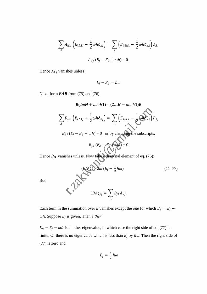
∑𝐴𝑘𝜆𝜆

(𝐸𝜆𝛿𝜆𝑗 − 1

2𝜔ℏ𝛿𝜆𝑗) = ∑(𝐸𝑘𝛿𝑘𝜆 −

1

2𝜔ℏ𝛿𝑘𝜆)𝐴𝜆𝑗

𝜆

𝐴𝑘𝑗 (𝐸𝑗 − 𝐸𝑘 + 𝜔ℏ) = 0.

Hence 𝐴𝑘𝑗 vanishes unless

𝐸𝑗 − 𝐸𝑘 = ℏ𝜔

Next, form BAB from (75) and (76):

B(2mH + 𝑚𝜔ℏ𝟏) = (2𝑚𝑯−𝑚𝜔ℏ𝟏)B

∑𝐵𝑘𝜆𝜆

(𝐸𝜆𝛿𝜆𝑗 + 1

2𝜔ℏ𝛿𝜆𝑗) = ∑(𝐸𝑘𝛿𝑘𝜆 −

1

2𝜔ℏ𝛿𝑘𝜆)𝐵𝜆𝑗

𝜆

𝐵𝑘𝑗 (𝐸𝑗 − 𝐸𝑘 + 𝜔ℏ) = 0 or by changing the subscripts,

𝐵𝑗𝑘 (𝐸𝑘 − 𝐸𝑗 + 𝜔ℏ) = 0

Hence 𝐵𝑗𝑘 vanishes unless. Now take a diagonal element of eq. (76):

(BA)𝑗𝑗 = 2m (𝐸𝑗 − 1

2ℏ𝜔) (11–77)

But

(𝐵𝐴)𝑗𝑗 =∑𝐵𝑗𝑘𝐴𝑘𝑗 .

𝜆

Each term in the summation over 𝜅 vanishes except the one for which 𝐸𝑘 = 𝐸𝑗 −

𝜔ℏ. Suppose 𝐸𝑗 is given. Then either

𝐸𝑘 = 𝐸𝑗 − 𝜔ℏ Is another eigenvalue, in which case the right side of eq. (77) is

finite. Or there is no eigenvalue which is less than 𝐸𝑗 by ℏ𝜔. Then the right side of

(77) is zero and

𝐸𝑗 = 1

2 ℏ𝜔

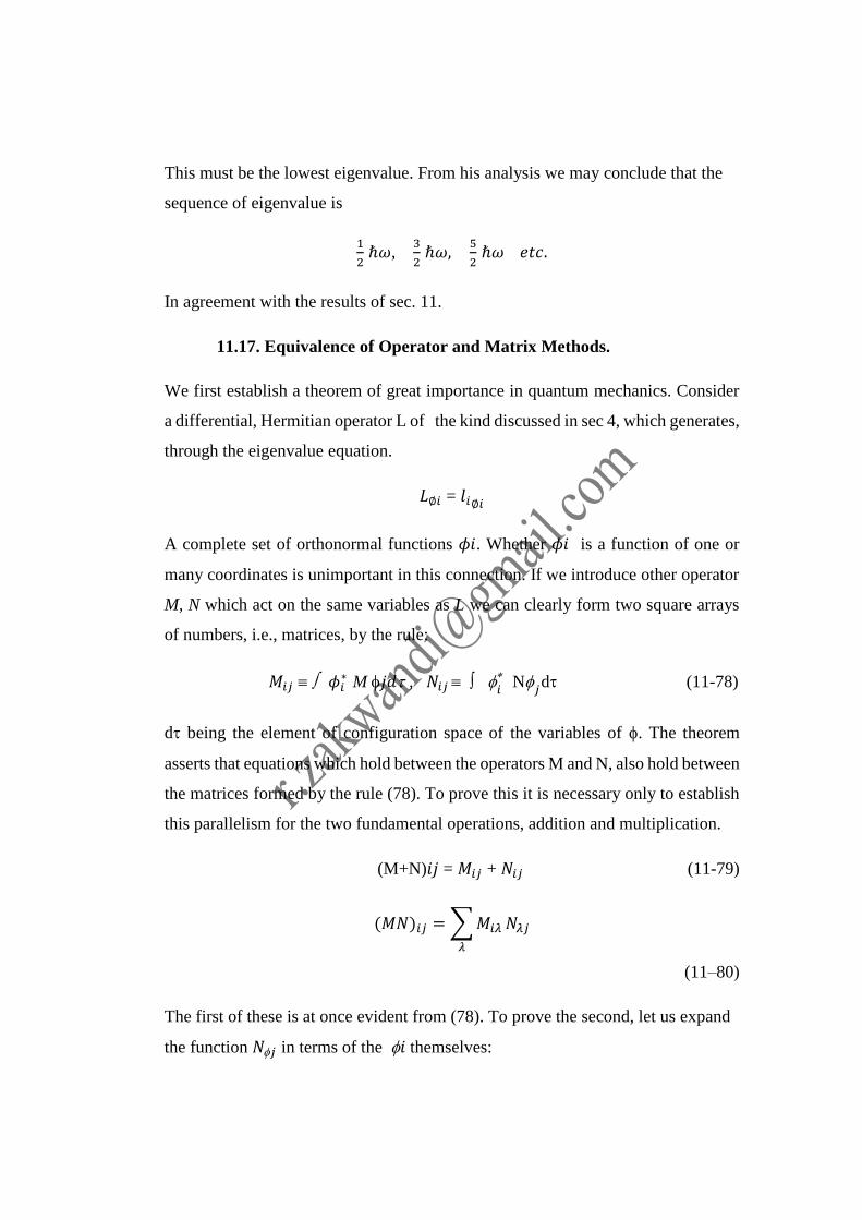
This must be the lowest eigenvalue. From his analysis we may conclude that the

sequence of eigenvalue is

1

2 ℏ𝜔,

3

2 ℏ𝜔,

5

2 ℏ𝜔 𝑒𝑡𝑐.

In agreement with the results of sec. 11.

11.17. Equivalence of Operator and Matrix Methods.

We first establish a theorem of great importance in quantum mechanics. Consider

a differential, Hermitian operator L of the kind discussed in sec 4, which generates,

through the eigenvalue equation.

𝐿∅𝑖 = 𝑙𝑖∅𝑖

A complete set of orthonormal functions 𝜙𝑖. Whether 𝜙𝑖 is a function of one or

many coordinates is unimportant in this connection. If we introduce other operator

M, N which act on the same variables as L we can clearly form two square arrays

of numbers, i.e., matrices, by the rule:

𝑀𝑖𝑗 𝜙𝑖 ∗ M 𝑗𝑑 , 𝑁𝑖𝑗

𝑖 N

𝑗d (11-78)

d being the element of configuration space of the variables of . The theorem

asserts that equations which hold between the operators M and N, also hold between

the matrices formed by the rule (78). To prove this it is necessary only to establish

this parallelism for the two fundamental operations, addition and multiplication.

(M+N)𝑖𝑗 = 𝑀𝑖𝑗 + 𝑁𝑖𝑗 (11-79)

(𝑀𝑁)𝑖𝑗 =∑𝑀𝑖𝜆

𝜆

𝑁𝜆𝑗

(11–80)

The first of these is at once evident from (78). To prove the second, let us expand

the function 𝑁𝑗 in terms of the 𝑖 themselves:

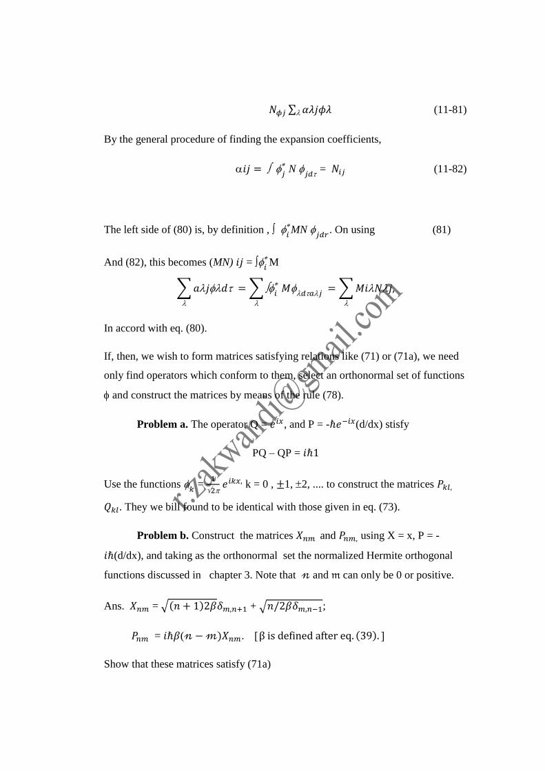
𝑁𝜙𝑗 ∑ 𝛼𝜆𝑗𝜙𝜆 (11-81)

By the general procedure of finding the expansion coefficients,

𝑖𝑗 = 𝑗 N

𝑗𝑑 = 𝑁𝑖𝑗 (11-82)

The left side of (80) is, by definition , 𝑖MN

𝑗𝑑𝑟. On using (81)

And (82), this becomes (MN) 𝑖𝑗 = 𝑖 M

∑𝑎𝑗𝑑

=∑ 𝑖

𝑀𝑑𝑎𝑗

=∑𝑀𝑖𝑁𝑗,

In accord with eq. (80).

If, then, we wish to form matrices satisfying relations like (71) or (71a), we need

only find operators which conform to them, select an orthonormal set of functions

and construct the matrices by means of the rule (78).

Problem a. The operator Q = 𝑒𝑖𝑥, and P = -ℏ𝑒−𝑖𝑥(d/dx) stisfy

PQ – QP = 𝑖ℏ1

Use the functions 𝑘 =

1

2 𝑒𝑖𝑘𝑥, k = 0 , ±1, 2, .... to construct the matrices 𝑃𝑘𝑙,

𝑄𝑘𝑙. They we bill found to be identical with those given in eq. (73).

Problem b. Construct the matrices 𝑋𝑛𝑚 and 𝑃𝑛𝑚, using X = x, P = -

𝑖ℏ(d/dx), and taking as the orthonormal set the normalized Hermite orthogonal

functions discussed in chapter 3. Note that 𝓃 and 𝔪 can only be 0 or positive.

Ans. 𝑋𝑛𝑚 = √(𝑛 + 1)2𝛽𝛿𝑚,𝑛+1 + √𝑛/2𝛽𝛿𝑚,𝑛−1;

𝑃𝑛𝑚 = 𝑖ℏ𝛽(𝓃 −𝓂)𝑋𝑛𝑚. β is defined after eq. (39).

Show that these matrices satisfy (71a)

It is interesting to note here that a Hermitian operator, defined by eq. (15),

generates a Hermitian matrix (cf. Sec. 11.10). for

𝑖 𝑃

𝑗𝑑 =

𝑗𝑃

𝑖d

Simply means

𝑃𝑖𝑗 = 𝑃𝑗𝑖

In our present notation.

The success of Heisenberg’s directions is now easily understood. The differential

operators which obey relations analogous to those prescribed for Heisenberg’s

matrices (71) are

𝑄𝑚 = 𝑞𝑚, 𝑃𝑚 = -𝑖ℏ𝜕

𝜕𝑞𝑚

In other words precisely the former, schrödinger operators. Suppose we select an

orthonormal set of functions ,𝑖, belonging to the operator L, and construct

(𝑄𝑚)𝑖𝑗 = 𝑖𝑄𝑚𝑗d

The fact that there are also others, like the ones considered in problem a, need not

disturb us here. The Schrödinger equation which results when they are used appears

different, to be sure, but reduces to its familiar form when a change of variable is

made.

When these matrices are substituted into the functional from H the result is the same

as if we had at once formed

𝐻𝑖𝑗 = ∫𝜙𝑖∗𝐻𝜙𝑗 𝑑𝜏

As follow from the theorem we have proved. But the only condition under which

this matrix can be diagonal is

𝐻𝜙𝑗 = 𝑐𝑜𝑛𝑠𝑡. 𝜙𝑗 (11–83)

That is to say, the 𝜙−functional must be chosen to be eigen functions of the

Hamiltonian H. The problem of making the matrix H diagonal is equivalent to

selecting the proper 𝜙𝑖, I. e., to solving the Schr��dinger equation. To see that the

diagonal elements of H are the permissible energies 𝐸𝑖 of the former theory, we

need only substitute 𝐻𝜙𝑗 = 𝐸𝑗𝜙𝑗 into (83), obtaining

𝐻𝑖𝑗 = 𝐸𝑖𝛿𝑖𝑗

It is easy to extend the Heisenberg theory beyond the limits of the present

development. The second postulate, eq. (8), is valid if P is interpreted as a matrix

and 𝜓𝜆 as a vector. In the terminology of chapter 10, the 𝜓𝜆 are then the

eigenvectors of the matrix P, and the 𝜌𝜆 are its eigenvalues. The relation of the

eigenvectors to the state functions is not difficult to see. Suppose we choose a basic

orthonormal set of functions, 𝜙𝑖. Expand the eigenfunctions ψ𝑖 appearing in the

operator equation

𝑃𝜓𝑖= 𝑝𝑖𝜓𝑖 (11–84)

In terms of them, viz.,

𝜓𝑖 =∑𝑎𝑖𝜆𝜙𝜆𝜆

.

Now multiply (84) by 𝜙𝑗∗ and integrate. We find immediately

∑𝑃𝑗𝜆 𝜆

𝑎𝑖𝜆 = 𝑝𝑖 𝑎𝑖𝑗

And conclude that the eigenvector Ψ𝑖 has as component the coefficients which

appear in its expansion in terms of the basic 𝜙. More explicitly,

𝜓𝑖 =

[ 𝑎𝑖1𝑎𝑖2𝑎𝑖3... ]

The last equation then reads (𝑃𝜓𝑖)𝑗 = 𝑃𝑖(𝜓𝑖)𝑗. If the basic set is identical with the

eigenfunctions of the operator P, eigenvector has only one non-vanishing

component.

Finally, even the third postulate, (14), may be retained in the Heisenberg

theory if its form is suitably changed. We interpret 𝜙 as a vector 𝜙 with components

𝑎𝑖, the 𝑎𝑖, being the coefficients in the expansion of the functions 𝜙 = in terms

of our basic 𝜙𝑖 (𝜙 without subscript here denotes an arbitrary state function, not

necessarily one of the set 𝜙𝑖 ), but 𝜙∗ not as the complex conjugate, but the

associate vector:

ϕ† = ( 𝑎1∗ 𝑎2

∗ 𝑎3∗ . . .)

P represents the matrix 𝑃𝑖𝑗 = ∫𝜙𝑖∗ 𝑃𝜙𝑗 𝑑𝜏 Eq. (14) must then be modified to

�� = ϕ† 𝑃ϕ

Which reads, when written more explicitly,

�� = ∑𝑎𝜆∗

𝜆𝜇

𝑃𝜆𝜇𝑎𝜇

When the 𝜙𝑖 are taken to be the aigenstates of the operator P, the matrix P becomes

diagonal, and

�� =∑𝑎𝜆∗

𝜆

𝑎𝜆𝑝𝜆

which is the same relation as was found the Schr��dinger theory under these

conditions.

Problem. Calculate the integral

∫ 𝓍𝜏∞

−∞

𝑒−𝓍2𝐻𝑛(𝑥)𝐻𝑚(𝑥)𝑑𝑥

By the methods of matrix mechanics. Let 𝜙𝑛 = 𝑐𝑛𝑒

−𝓍2/2 𝐻𝑛 (𝓍), 𝜙𝑚 = 𝑐𝑚

𝑒−𝓍2/2𝐻𝑛 (𝓍) , where 𝑐𝑛, 𝑐𝑚 are normalizing factors, and note that, aside from

normalizing factors, the integral is the matrix element ( 𝑥𝜏)𝑛𝑚. Now 𝑥𝜆𝜇 is given

by eq. (3-39); this may be used in calculating

(𝓍𝜏)𝑛𝑚 = ∑ 𝓍𝑛𝜆𝓍𝜆𝜇𝓍𝜇𝜈⋯𝓍𝜎𝑚𝜆,𝜇,𝜈,⋯𝜎

APPROXIMATION METHODS FOR SOLVING EIGENVALUE

PROBLEMS

11.18. Variantional (Ritz) Method.

In chapter 8 we showed that the differential equation 𝐿(𝑢) + 𝜆𝑤𝑢 = (𝑝𝑢′)′ −

𝑞𝑢 + 𝜆𝑤𝑢 = 0 is the necessary (though not sufficient!) condition upon u if it is to

minimize the integral Ʌ(𝑢) = ∫(𝑝𝑢′2 + 𝑞𝑢2) 𝑑𝑥 . Futhermore, it was seen that

Ʌ(𝒖) could be transformed (cf. eq. 8–37) by simple steps to −∫𝑢𝐿(𝑢)d 𝓍. The

theory in this simple form is applicable to every one-dimensional Schr��dinger

equation, for in that case the Hamiltonian operator H = -(ℏ2/2m) (𝑑2/𝑑𝑥2) + V (𝑥)

is of the form –L if only we identify p with ℏ2/2m and q with V. Hence we may at

once say that the Schrodinger equation is the necessary condition upon 𝜓 so that

the integral

∫𝜓𝐻𝜓d

Shall be a minimum. The one-dimensional variation theory may also be applied,

though in a somewhat more cumbersome manner, to every ordinary differential

equation to which the multi-dimensional Schrödinger equation gives rise on

separation of variables. It is possible, however, to prove a far more general theorem

which is of utmost utility in numerous problems of applied mathematics, a theorem

of which the former statement is a special case.

Let P be a Hermitian operator. We wish to find the normalized function 𝜓

which will make the integral

∫ 𝜓𝑃𝜓d

A minimum. The integration extends, as usual over configuration space, and we

shall assume for the sake of definiteness that is a finite portion of configuration

space. Certainly, the necessary condition upon 𝜓 is that

𝛿 {∫𝜓𝑃𝜓𝑑 − ∫𝜓𝜓𝑑}

Shall vanish; is an undetermined ( Lagrangian) multiplier (cf. Sec. 6.5). Now the

variation symbol and the integral sign are commutable in this expression because

the limits of the integration are supposed finite and fixed. Hence we have

∫𝛿𝜓. 𝑃𝜓𝑑 + ∫𝜓. 𝛿(𝑃𝜓)𝑑 − 𝜆 ∫ 𝛿𝜓. 𝜓𝑑 − 𝜆 ∫𝜓𝛿𝜓𝑑 = 0 (11-85)

The second integral in this expression may be transformed in two steps.

Firts, 𝛿(𝑃𝜓) may be replaced by 𝑃(𝛿𝜓) since the operator P suffers no variation.

Second because P is Hermitian and both 𝜓 𝑎𝑛𝑑 𝛿𝜓 are acceptable functions,

∫𝜓𝑃(𝛿𝜓)d = ∫𝛿𝜓. 𝑃𝜓d. Eq. (85) therefore reads

∫𝛿𝜓(𝑃𝜓 − 𝜆𝜓)d +∫ 𝛿𝜓(𝑃𝜓− 𝜆𝜓)d =0 (11-86)

Here 𝛿𝜓 is an entirely arbitrary functions. Let us take it to be real, so that 𝛿𝜓

= 𝛿𝜓. 𝐸𝑞. (86) can be satisfied only if

P𝜓 − 𝜆𝜓 + 𝑃𝜓− 𝜆𝜓 = 0

On the other hand, if we take 𝛿𝜓 to be imaginary, so that 𝛿𝜓 = −𝛿𝜓, we conclude

𝑃𝜓 − 𝜆𝜓 − 𝑃𝜓 + 𝜆𝜓 = 0

Addition of the last two equations yields

𝑃𝜓 = 𝜆𝜓

Subtraction gives

𝑃𝜓 = 𝜆𝜓

We have shown that, if

𝛿 ∫𝜓𝑃𝜓𝑑 = 0 (11-87)

For normalized 𝜓, this functionmust satisfy the eigenvalue equation

𝑃𝜓 = 𝜆𝜓 (11-88)

Which also automatically determines 𝜆. Whether, when (88) is satisfied, the

minimum of, or indeed the integral, ∫𝜓𝑃𝜓𝑑, actually exists, is a point we have

not investigated. It is customary in physics not to worry about these eventualities,

for they are difficult to discuss. The mathematical equivalence of the minimal

property of the integral and eq. (88) is usually taken as a matter of faith.

If 𝜓 satisfies eq. (88), then∫𝜓𝑃𝜓𝑑, = 𝜆 . From what has been said it follows,

therefore, that the integral ∫𝜑𝑃𝜑𝑑 computed with a function different from the

minimizing 𝜓, cannot be smaller than𝜆. But here a slight complication arises, for

there are many eigenvalues𝜆. All that we can really say is that for a function 𝜑 in

the “neighborhood” of 𝜓𝑖, the integral will not be greater than 𝜆𝑖. Certainly,

however,

∫𝜑𝑃𝜑𝑑 =≥ 𝜆0 (11-89)

If 𝜑 is any analytic and continuous function19 and 𝜆0 the lowest eigenvalue.

19 Restriction to function with a certain number of derivatives is necessary because P is in general a differential operator, and P 𝜑 must have meaning

The Ritz method, 20 named after its inventor, is a systematic procedure,

based upon the foregoing variational considerations, for solving the eigenvalue

equation (88) by substituting into the integral in (87) a suitable sequence of function

which causes the integral to converge upon the value 𝜆. Instead of presenting the

method in its original form, we shall here work out some of its features in a manner

more directly adapted to the needs of quantum mechanics, and with a slight loss of

the lowest (normal state) energy of physical energy of physical or chemical system,

hence with identify at once the operator P in (89) with the hamiltionan H.

The simples way of finding an approximation to the lowest wnwrgy of the system

in to use (89) directly. Sometimes a good guess can be made as to the general form

of the true state function , a from which may allow the inclution of one or more

arbitrary parameters. The integral in (89) is then computed with this function, and

the result is minimized with respect to the parameters. An example with the clarify

the methode.

11.19. example: normal state of the helium atom. The helium atom consists

of two electron moving in the field of the nucleus of charge 2e and at the same time

repelling each other. We consider the nucleus as stationary and denote the distances

of the two electrons from it by r1 and r2 respectively; r12 is the interelectronic

distance. The potential energy is – 2𝑒2(1/𝑟1 + 1/𝑟2) + 𝑒2/𝑟12, and the scrodinger

equation.

𝐻 = {−ℎ2

2𝑚(∇1

2 + ∇22) − 2𝑒2(1/𝑟1 + 1/𝑟2) + 𝑒2/𝑟12} = 𝐸 (11-90)

A subscript on the symbol ∇ indicates that the laplacian is to be taken with respect

to the respect to the coordinates labeled by the subscript. If the term 𝑒2/𝑟12 where

absent eq. (90) would be sparable, for then the operator H would be to the sum of

two helium – ion Hamiltonians, 𝐻 = 𝐻1 + 𝐻2, the first acting on the coordinates of

electron 1, the second on those of electrons 2. But the equation.

20 Ritz, W ., J . f. Reine und angew. Math .135, 1 (1909); Courant-Hilbert, p. 150.

(𝐻1 + 𝐻2) = 𝐸

May be separated of substitution of = 𝑢(1)𝑣(2), where 𝑢(1) stand for a function

of the space coordinates of electron 1, the second on those of electron 2. But the

equation.

𝐻1𝑢(1)

𝑢(1)+𝐻2𝑢(2)

𝑢(2)= 𝐸, a constant

Which indicates that 𝐻1𝑢(1) = 𝑒1𝑢(1); 𝐻2𝑣(2) = 𝐸2𝑣(2); 𝐸1 + 𝐸2 = 𝐸. But the

first two of these are simply Schrὄdinger equations for the singly charged helium

ion, whose solutions we already know. (Cf. eq. 67a) since we wish to find the lowest

energy of our system, we identify the functions as follow:

𝑢(1) = (𝑍3

𝜋𝑎03)

1/2 𝑒−𝑟1/𝑎0. 𝑣(2) = (𝑍3

𝜋𝑎03)

1/2 𝑒−𝑟1/𝑎0

And is the product of these.

The correct solution of eq. (90) is certainly not of this exact from because

of the “interaction term” 𝑒2/𝑟12, whose effect on one would expext to be very

complicated indeed. Aside from other changes, it will couse to depend or r12

expicitl. But from a physical point of view, the repulsion between the electrons will

cause both of them to be, on the average, farther away from the nucleus then if the

repulsion were absent. This would mean that the function 𝑢 and 𝑣 are in error with

respect to the scale factor 𝑍/𝑎0. If this were smaller, a more extended probability

distribution would result. (for the helium ion Z = 2) it woud seen expendient,

therefore, that we take as our “trial” function in the variational procedure teh

function = 𝑢(1)𝑣(2) but with an undertermined Z.

In calculating

∫ 𝐻𝑑𝑟 (11.90)

It is well to have available the differential equation whose solution are 𝑢 and 𝑣:

−ℎ2

2𝑚∇12𝑢(1) =

𝑍𝑒2

𝑟1𝑢(1) + 𝑍2𝐸𝐻𝑢(1), 𝑣(2) = 𝑢(2) (11-91)

Here 𝐸𝐻 is the energy is the normal hydrogen atom, 𝐸𝐻 = −𝑒2/2𝑎0(=

−13.53 𝑒. 𝑣𝑜𝑙𝑡𝑠). the differential 𝑑𝑟 in (91) represent, of course, the product of the

volume element for then two electrons. When H is taken from (90), we find, using

(92) and the fact that u is normalized,

∫ 𝐻𝑑𝑟 = 2𝑍2𝐸𝐻 + (𝑍 − 2)𝑒2 ∫ (

1

𝑟1+

1

𝑟2) 2𝑑𝑟 + 𝑒2 ∫

2

𝑟12𝑑𝑟 (11 – 92)

The integral

∫2

𝑟1𝑑𝑟 = ∫

𝑢2(1)

𝑟1𝑑𝑟1. ∫ 𝑢

2(2)𝑑𝑟2 = ∫𝑢2(1)

𝑟1. 𝑟12𝑑𝑟1 sin 𝜃𝑑𝜃𝑑𝜑

Is easily computed directly. It has, in fact, already been evaluated (cf. sec. 3.11,

example) and found to be 𝑍/𝑎0. The other integral, ∫2

𝑟1𝑑𝑟, has the same value.

We leave the evaluation of 𝑒2 ∫2

𝑟1𝑑𝑟 for later; its value is −

5

4𝑍𝐸𝐻 . Hence, eq.

(93) becomes

∫ 𝐻𝑑𝑟 = 2𝑍𝐸𝐻 + (𝑍 − 2). 2𝑍𝑒2

𝑎0−5

4𝑍𝐸𝐻 (11 – 93)

= 𝑍 [2𝑍 − 4(𝑍 − 2) −5

4] 𝐸𝐻

The symbol ℋ𝑖𝑗 in place of Hi j is to remind the reader of the fact that the matrix ℋ

dose not possess the simple properties of H because the former is not constructed

with an orthonormal, complete set of functions. The denominator in the expression

for E is needed to normalize the function ∅. According to the variantional principle,

E ≥ E0, the lowest energy state of the system.

We wish to find the condition that E shall be a minimum, and the minimum value

of E. insertion of (94) gives

𝐸 = ∑ 𝛼𝜆∗𝛼µℋ𝜆𝜇

𝑛𝜆,µ=1 / ∑ 𝛼𝜆

∗𝛼µ∆𝜆𝜇𝜆𝜇 (11 – 9)

This expression will be an extremum, and we hope a minimum, if E is so adjusted

that 𝜕𝐸

𝜕𝛼𝜅∗ and

𝜕𝐸

𝜕𝛼𝜅 are zero for every k from 1 to n. let us take the derivative with

respect to 𝛼𝜅∗ on both sides of last equation after is it written in form

𝐸 ∑𝛼𝜆∗𝛼µ∆𝜆𝜇

𝜆𝜇

= ∑𝛼𝜆∗𝛼µℋ𝜆𝜇

𝜆𝜇

The result is

𝜕𝐸

𝜕𝛼𝜅∗ ∑ 𝛼𝜆

∗𝛼𝜇∆𝜆𝜇 + 𝐸 ∑ 𝛼𝜇Δ𝜅𝜇 = ∑ 𝛼𝜇ℋ𝜅ì, 𝜅 = 1,2, … , 𝑛𝜇𝜇𝜆𝜇 (11 – 95)

When first term is omitted (𝜕𝐸

𝜕𝛼𝜅∗ = 0) the reminder of the equation represent the

condition that E shall be a minimum. Differentiation of (95) with respect to 𝛼𝜅 leads

in a similar way to

𝐸 ∑𝛼𝜆∗∆𝜆𝜅

𝜆

= ∑𝛼𝜆∗ℋ𝜆𝜅

𝜆

An equation which is simply the conjugate of the former. Both may conveniently

be written

∑ 𝛼𝜇(ℋ𝜅𝜇 − Δ𝜅𝜇𝐸) = 0, 𝑘 = 1,2, . . . , 𝑛𝜇 (11-96)

If this system of equation is to have a solution different from the trivial one,

every 𝛼𝜇 = 0, then determinant constructed from the coefficients of the 𝛼𝜇 must

vanish. Thus

||

ℋ11 − Δ11𝐸 ℋ12 − Δ12𝐸 … ℋ1𝑛 − Δ1𝑛𝐸ℋ21 − Δ21𝐸 ℋ22 − Δ22𝐸 … ℋ2𝑛 − Δ2𝑛𝐸…………………………………………………… .…………………………………………………… .ℋ𝑛1 − Δ𝑛1𝐸 ℋ𝑛2 − Δ𝑛2𝐸 … ℋ𝑛𝑛 − Δ𝑛𝑛𝐸

|| = 0 (11-97)

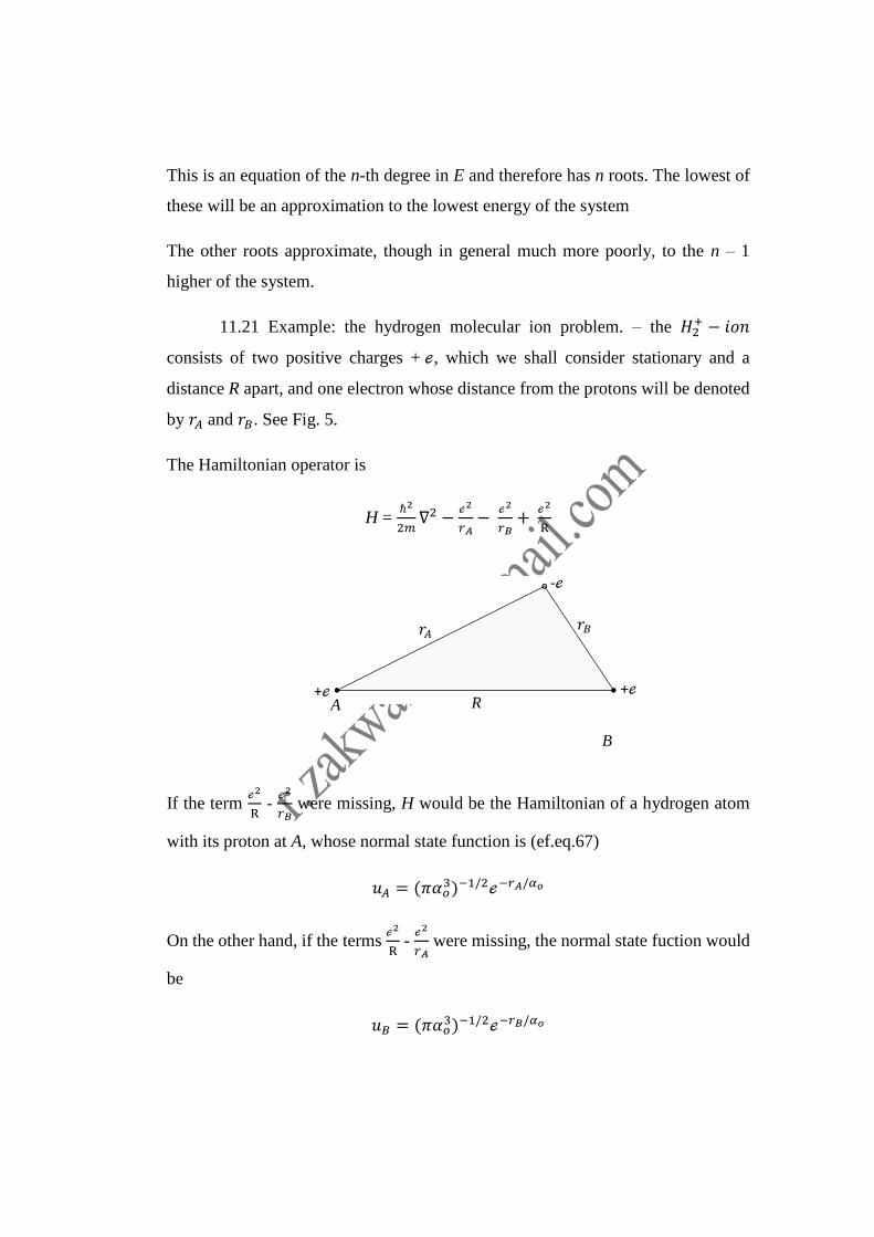
+ℯ +ℯ

𝑟𝐴 𝑟𝐵

R

A

This is an equation of the n-th degree in E and therefore has n roots. The lowest of

these will be an approximation to the lowest energy of the system

The other roots approximate, though in general much more poorly, to the n – 1

higher of the system.

11.21 Example: the hydrogen molecular ion problem. – the 𝐻2+ − 𝑖𝑜𝑛

consists of two positive charges + ℯ, which we shall consider stationary and a

distance R apart, and one electron whose distance from the protons will be denoted

by 𝑟𝐴 and 𝑟𝐵. See Fig. 5.

The Hamiltonian operator is

H = ℏ2

2𝑚∇2 −

ℯ2

𝑟𝐴−

ℯ2

𝑟𝐵+

ℯ2

R

If the term ℯ2

R - ℯ2

𝑟𝐵 were missing, H would be the Hamiltonian of a hydrogen atom

with its proton at A, whose normal state function is (ef.eq.67)

𝑢𝐴 = (𝜋𝛼𝜊3)−1/2ℯ−𝑟𝐴/𝛼𝜊

On the other hand, if the terms ℯ2

R - ℯ2

𝑟𝐴 were missing, the normal state fuction would

be

𝑢𝐵 = (𝜋𝛼𝜊3)−1/2ℯ−𝑟𝐵/𝛼𝜊

B

-ℯ

From a physical point of view one of these solutions is as good as the other: 𝑢𝐴

implies that the electron is entirely attached to proton A, 𝑢𝐵 that it is attached to

proton B. Neither is the ease. Let us see what happens if we take for variation

function ∅ a linear combination of 𝑢𝐴 and 𝑢𝐵. We put

∅ = 𝛼𝐴𝑢𝐴 + 𝛼𝐵𝑢𝐵

Using letters as subscripts rather than the number indices which appear in (94).21

The lowest energy is at once obtained as the lowest root of (97) which takes the

simple form

|ℋ𝐴𝐴 − ∆𝐴𝐴𝐸 ℋ𝐴𝐵 − ∆𝐴𝐵𝐸ℋ𝐵𝐴 − ∆𝐵𝐴𝐸 ℋ𝐵𝐵 − ∆𝐵𝐵𝐸

| = 0 (11-98)

in more complicated molecules it is well to label electron by numbers, nuclei letters.

We here follow this convention. Now ∆𝐴𝐴= ∫𝑢𝐴∗𝑢𝐴𝑑𝜏 = Δ𝐵𝐵 = 1, because 𝑢𝐴 and

𝑢𝐵 are normalized. They are not orthogonal, but ∆𝐴𝐵 = ∆𝐵𝐴. Similar, ℋ𝐴𝐵 =

∫𝑢𝐴𝐻𝑢𝐵𝑑𝜏 = ℋ𝐵𝐴 𝑑𝑎𝑛 ℋ𝐵𝐵 = ℋ𝐴𝐴 since H is insensitive to an interchange of

I A and B. with these simplifications the two roots of (98) are found to be

𝐸1 =ℋ𝐴𝐴+ℋ𝐴𝐵

1+∆𝐴𝐵 𝐸2 =

ℋ𝐴𝐴−ℋ𝐴𝐵

1−∆𝐴𝐵 (11-99)

The ∅ -functions corresponding to these energies are obtained from (96):

𝛼𝐴(ℋ𝐴𝐴 − 𝐸) + 𝛼𝐵(ℋ𝐴𝐵 − ∆𝐴𝐵𝐸) = 0

𝛼𝐴(ℋ𝐵𝐴 − ∆𝐵𝐴𝐸) + 𝛼𝐵(ℋ𝐵𝐵 − 𝐸) = 0

On inserting E = E1 we get 𝛼𝐴 = 𝛼𝐵 ; hence the corresponding

∅1 = 𝑐1(𝑢𝐴 + 𝑢𝐵)

If ∅1 is to normalized, 𝑐1 = [2(1 + ∆𝐴𝐵)]-1/2 . if E2 is inserted in (99), we find 𝛼𝐵

= - 𝛼𝐴, so that

∅2 = 𝑐2(𝑢𝐴 − 𝑢𝐵)

The normalizing factor is in this case 𝑐2 = [2(1 − ∆𝐴𝐵)]-1/2.

The remainder of the work is the computation of the three quantities ∆𝐴𝐵, ℋ𝐴𝐴 and

ℋ𝐴𝐵. It involves nothing new and will be left to the reader. The integrals are most

easily evaluated in spheroidal coordinates (cf.eq. 5-40). 𝜉 = 𝑟𝐴− 𝑟𝐵

𝑅, 𝜂 =

𝑟𝐴− 𝑟𝐵

𝑅 and

𝜑, the latter measured around R. In terms of these

𝑑𝜏 = 𝑅3

8(𝜉2 − 𝜂2)𝑑𝜉𝑑𝜂𝑑𝜑, 𝑑𝑎𝑛 𝑢𝐴𝑢𝐵 = (𝜋𝛼0

3)−1ℯ−(𝑅/𝛼𝑂)𝜉

1 ≤ 𝜉 < ∞; −1 ≤ 𝜂 ≤ 1

the following results will be found:

∆𝐴𝐵= ℯ−𝜌(1 + 𝜌 +

𝜌2

3

ℋ𝐴𝐴 = 𝐸𝐻 +ℯ2

𝑅+ 𝐽

𝐽 = −∫𝑢𝐴ℯ2

𝑟𝐵𝑢𝐴 𝑑𝜏 = −

ℯ2

𝑅[1 − ℯ−2𝜌(1 + 𝜌)]

ℋ𝐴𝐵 = (𝐸𝐻 +ℯ2

𝑅)∆𝐴𝐵 + 𝐾,

𝐾 = − ∫ 𝑢𝐴ℯ2

𝑟𝐴𝑢𝐵 𝑑𝜏 = −

ℯ2

𝑅ℯ−𝜌(𝜌 + 𝜌2) (11-100 )

The parameter 𝜌 ≡𝑅

𝛼0; 𝐸𝐻 is defined as in sec. 19. The quantities J and K are of

interest. According to its definitions, J represent the coulomb attraction energy

between a negative charge of density 𝑢𝐴2 and the proton B. the integral K has no

such simple interpretation; it is called an exchange integral. Its importance is best

appreciated if E1 and E2 are written more explicitly with the use of (100):

𝐸1 = 𝐸𝐻 + ℯ2

𝑅+

𝐽 + 𝐾

1 + ∆𝐴𝐵

𝐸2 = 𝐸𝐻 + ℯ2

𝑅+

𝐽 − 𝐾

1 − ∆𝐴𝐵

Because K is negative, 𝐸1 is the lower root, had we omitted the function 𝑢𝐵 from

our trial function ∅, the variantional result would have been

𝐸 = 𝐸𝐻 + ℯ2

𝑅+ 𝐽

𝐸1 is lower than this by virtue of the presence of K (and of course ∆𝐴𝐵). But in

classical parlance, a lower energy must be regarded as due to the presence of

additional attractive forces between the constituents of the system, i.e., a hydrogen

atom and a proton. These forces would be given by 𝜕𝐾

𝜕𝑅; they are commonly called

exchange forces. They possess no classical interpretation; their significance is

rooted entirely in the variational method through which they arise.

Of course 𝐸1 is only an approximation to the true energy, which is lower for every

R. Its most important feature is that it possesses a minimum, which explains the

stability of the 𝐻2+ ion. Classical mechanics would yield no minimum and is

therefore incompetent to account for the existence of this ion. A detailed

comparison of 𝐸1 with the experimental energy is given in pauling and Wilson.21

Problem Let 𝑢0, 𝑢1, 𝑢2, be the three lowest energy states of the simple harmonic

oscillator, 𝐻0 its Hamiltonian. The Hamiltonian for an oscillator in an electric field

is H = 𝐻0 + 𝑘𝑥, where k is a constant. Calculate by the variational method the

lowest energy of this system, using as trial functions (a) 𝑢0, (b) 𝑎0 𝑢0 +

𝑎1 𝑢1 (𝑐) 𝑎0 𝑢0 + 𝑎1 𝑢1 + 𝑎2 𝑢2 .

21 pauling and Wilson, loc. cit.

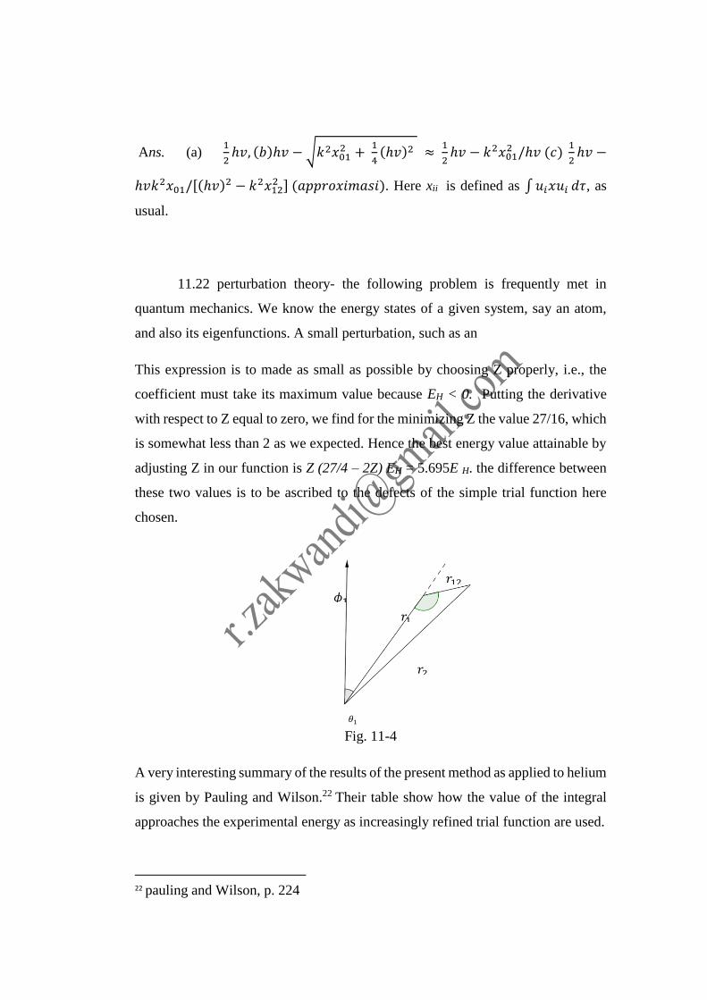
Ans. (a) 1

2ℎ𝑣, (𝑏)ℎ𝑣 − √𝑘2𝑥01

2 + 1

4(ℎ𝑣)2 ≈

1

2ℎ𝑣 − 𝑘2𝑥01

2 /ℎ𝑣 (𝑐) 1

2ℎ𝑣 −

ℎ𝑣𝑘2𝑥01/[(ℎ𝑣)2 − 𝑘2𝑥12

2 ] (𝑎𝑝𝑝𝑟𝑜𝑥𝑖𝑚𝑎𝑠𝑖). Here xii is defined as ∫𝑢𝑖𝑥𝑢𝑖 𝑑𝜏, as

usual.

11.22 perturbation theory- the following problem is frequently met in

quantum mechanics. We know the energy states of a given system, say an atom,

and also its eigenfunctions. A small perturbation, such as an

This expression is to made as small as possible by choosing Z properly, i.e., the

coefficient must take its maximum value because EH < 0. Putting the derivative

with respect to Z equal to zero, we find for the minimizing Z the value 27/16, which

is somewhat less than 2 as we expected. Hence the best energy value attainable by

adjusting Z in our function is Z (27/4 – 2Z) EH = 5.695E H. the difference between

these two values is to be ascribed to the defects of the simple trial function here

chosen.

Fig. 11-4

A very interesting summary of the results of the present method as applied to helium

is given by Pauling and Wilson.22 Their table show how the value of the integral

approaches the experimental energy as increasingly refined trial function are used.

22 pauling and Wilson, p. 224

𝜙1

𝑟1

𝑟2

𝑟12

𝜃1

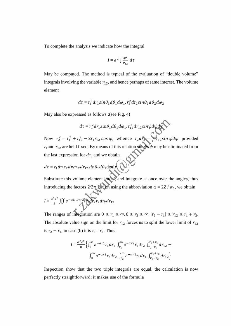
To complete the analysis we indicate how the integral

I = ℯ2 ∫𝜙2

𝑟12 𝑑𝜏

May be computed. The method is typical of the evaluation of “double volume”

integrals involving the variable 𝑟12, and hence perhaps of same interest. The volume

element

𝑑𝜏 = 𝑟12𝑑𝑟1𝑠𝑖𝑛𝜃1𝑑𝜃1𝑑𝜑1. 𝑟2

2𝑑𝑟2𝑠𝑖𝑛𝜃2𝑑𝜃2𝑑𝜑2

May also be expressed as follows :(see Fig. 4)

𝑑𝜏 = 𝑟12𝑑𝑟1𝑠𝑖𝑛𝜃1𝑑𝜃1𝑑𝜑1. 𝑟12

2 𝑑𝑟12𝑠𝑖𝑛𝜓𝑑𝜓𝑑𝜒

Now 𝑟22 = 𝑟1

2 + 𝑟122 − 2𝑟1𝑟12 𝑐𝑜𝑠 𝜓, whence 𝑟2𝑑𝑟2 = 𝑟1𝑟12𝑠𝑖𝑛 𝜓𝑑𝜓 provided

𝑟1and 𝑟12 are held fixed. By means of this relation sin 𝜓𝑑𝜓 may be eliminated from

the last expression for 𝑑𝜏, and we obtain

𝑑𝜏 = 𝑟1𝑑𝑟1𝑟2𝑑𝑟2𝑟12𝑑𝑟12𝑠𝑖𝑛𝜃1𝑑𝜃1d𝜑d𝜒

Substitute this volume element into I, and integrate at once over the angles, thus

introducing the factors 2.2𝜋 .2𝜋 . on using the abbreviation 𝛼 = 2Z / 𝛼0, we obtain

I = 𝛼6ℯ2

8∭ℯ−𝛼(𝑟1+𝑟2)𝑟1𝑑𝑟2𝑟2𝑑𝑟2𝑑𝑟12

The ranges of integration are 0 ≤ 𝑟1 ≤ ∞, 0 ≤ 𝑟2 ≤ ∞; |𝑟2 − 𝑟1| ≤ 𝑟12 ≤ 𝑟1 + 𝑟2.

The absolute value sign on the limit for 𝑟12 forces us to split the lower limit of 𝑟12

is 𝑟2 − 𝑟1, in case (b) it is 𝑟1 - 𝑟2. Thus

I = 𝛼6ℯ2

8{∫ ℯ−𝛼𝑟1𝑟1𝑑𝑟1

∞

0 ∫ ℯ−𝛼𝑟2𝑟2𝑑𝑟2 ∫ 𝑑𝑟12 +

𝑟2+𝑟1

𝑟2−𝑟1

∞

𝑟1

∫ ℯ−𝛼𝑟2𝑟2𝑑𝑟2 ∫ ℯ−𝛼𝑟1𝑟1𝑑𝑟1∞

𝑟2

∞

0 ∫ 𝑑𝑟12𝑟1+𝑟2

𝑟1−𝑟2}

Inspection show that the two triple integrals are equal, the calculation is now

perfectly straightforward; it makes use of the formula

∫ ℯ−𝑝𝑥𝑥𝑛𝑑𝑥∞

0

= 𝑝−(𝑛+1)𝑛!

And leads to the result

I = 5

8 𝑍

ℯ2

𝛼0=

5

4𝑍𝐸𝐻

Which was used above.

11.20 the method of linier variation functions.

It is often convenient to use as the trial function 𝜙 in ∫𝜙∗𝐻𝜙 𝑑𝜏 a linier

combination of definite function 𝑢𝑖 which are judged suitable for the problem at

hand. The coefficients appearing in the linier combination may then be tread as

variable parameters thus, assume

𝜙 = ∑𝛼𝜆𝑢𝜆

𝑛

𝜆=1

Where the u’s need not form an orthonormal set. We define

∫𝑢𝑖∗𝑢𝑗 𝑑𝜏 = Δ𝑖𝑗, ∫𝑢𝑖

∗𝐻𝑢𝑗 𝑑𝜏 = ℋ𝑖𝑗 , E ∫𝜙∗𝐻𝜙𝑑𝜏

∫𝜙∗𝜙𝑑𝜏

Electric or magnetic field, is now imposed; this changes, presumably by slight

amounts, both energy and state function. Mathematically, the situation is described

in this way. We know the solutions and eigenvalues of

𝐻0𝜓𝑖 = 𝐸𝑖0𝜓𝑖 (11–101)

Where 𝐻0 is the “unperturbed” Hamiltonian. We wish to find solution and

eigenvalues of

𝐻𝜙𝑖 = 𝐸𝑖𝜙𝑖, 𝐻0 + 𝐻′ (11–102)

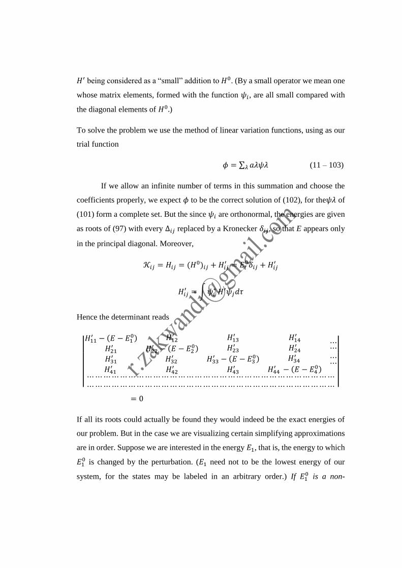
𝐻′ being considered as a “small” addition to 𝐻0. (By a small operator we mean one

whose matrix elements, formed with the function 𝜓𝑖, are all small compared with

the diagonal elements of 𝐻0.)

To solve the problem we use the method of linear variation functions, using as our

trial function

𝜙 = ∑ 𝑎𝜆𝜓𝜆𝜆 (11 – 103)

If we allow an infinite number of terms in this summation and choose the

coefficients properly, we expect 𝜙 to be the correct solution of (102), for the𝜓𝜆 of

(101) form a complete set. But the since 𝜓𝑖 are orthonormal, the energies are given

as roots of (97) with every Δ𝑖𝑗 replaced by a Kronecker 𝛿𝑖𝑗, so that E appears only

in the principal diagonal. Moreover,

𝒦𝑖𝑗 = 𝐻𝑖𝑗 = (𝐻0)𝑖𝑗 + 𝐻𝑖𝑗′ = 𝐸𝑖

0𝛿𝑖𝑗 + 𝐻𝑖𝑗′

𝐻𝑖𝑗′ = ∫𝜓𝑖

∗𝐻′𝜓𝑗𝑑𝜏

Hence the determinant reads

|

|

𝐻11′ − (𝐸 − 𝐸1

0)

𝐻21′

𝐻31′

𝐻41 ′

𝐻12′

𝐻22′ − (𝐸 − 𝐸2

0)

𝐻32 ′

𝐻42′

𝐻13′

𝐻23′

𝐻33′ − (𝐸 − 𝐸3

0)

𝐻43′

𝐻14′

𝐻24′

𝐻34 ′

𝐻44 ′ − (𝐸 − 𝐸4

0)

⋯⋯⋯⋯

⋯⋯⋯⋯⋯⋯⋯⋯⋯⋯⋯⋯⋯⋯⋯⋯⋯⋯⋯⋯⋯⋯⋯⋯⋯⋯⋯⋯⋯⋯⋯⋯⋯⋯⋯⋯⋯⋯⋯⋯⋯⋯⋯⋯⋯⋯⋯⋯⋯⋯⋯⋯⋯⋯⋯⋯⋯⋯⋯⋯

|

|

= 0

If all its roots could actually be found they would indeed be the exact energies of

our problem. But in the case we are visualizing certain simplifying approximations

are in order. Suppose we are interested in the energy 𝐸1, that is, the energy to which

𝐸10 is changed by the perturbation. (𝐸1 need not to be the lowest energy of our

system, for the states may be labeled in an arbitrary order.) If 𝐸10 is a non-

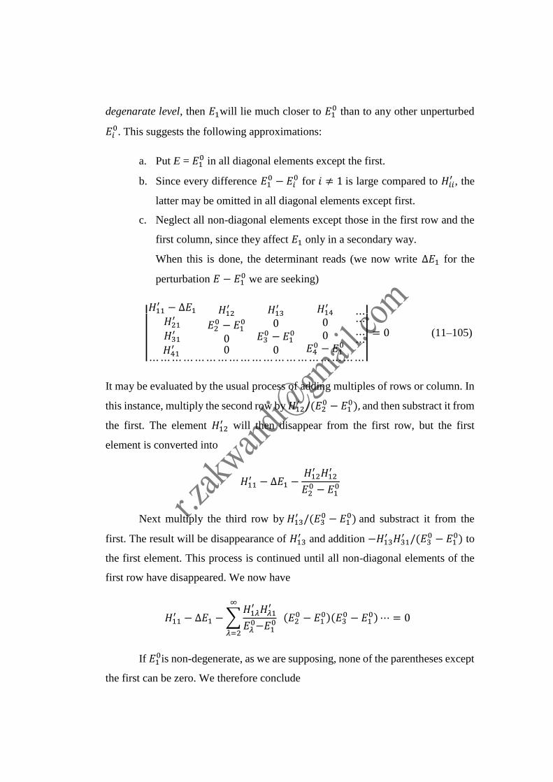
degenarate level, then 𝐸1will lie much closer to 𝐸10 than to any other unperturbed

𝐸𝑖0. This suggests the following approximations:

a. Put E = 𝐸10 in all diagonal elements except the first.

b. Since every difference 𝐸10 − 𝐸𝑖

0 for 𝑖 ≠ 1 is large compared to 𝐻𝑖𝑖′ , the

latter may be omitted in all diagonal elements except first.

c. Neglect all non-diagonal elements except those in the first row and the

first column, since they affect 𝐸1 only in a secondary way.

When this is done, the determinant reads (we now write Δ𝐸1 for the

perturbation 𝐸 − 𝐸10 we are seeking)

||

𝐻11′ − Δ𝐸1𝐻21′

𝐻31′

𝐻41 ′

𝐻12′

𝐸20 − 𝐸1

0

00

𝐻13′

0𝐸30 − 𝐸1

0

0

𝐻14′

00

𝐸40 − 𝐸1

0

⋯⋯⋯⋯

⋯⋯⋯⋯⋯⋯⋯⋯⋯⋯⋯⋯⋯⋯⋯⋯⋯⋯⋯

|| = 0 (11–105)

It may be evaluated by the usual process of adding multiples of rows or column. In

this instance, multiply the second row by 𝐻12′ /(𝐸2

0 − 𝐸10), and then substract it from

the first. The element 𝐻12′ will then disappear from the first row, but the first

element is converted into

𝐻11′ − Δ𝐸1 −

𝐻12′ 𝐻12

′

𝐸20 − 𝐸1

0

Next multiply the third row by 𝐻13′ /(𝐸3

0 − 𝐸10) and substract it from the

first. The result will be disappearance of 𝐻13′ and addition −𝐻13

′ 𝐻31′ /(𝐸3

0 − 𝐸10) to

the first element. This process is continued until all non-diagonal elements of the

first row have disappeared. We now have

𝐻11′ − Δ𝐸1 −∑

𝐻1𝜆′ 𝐻𝜆1

′

𝐸𝜆0−𝐸1

0

∞

𝜆=2

(𝐸20 − 𝐸1

0)(𝐸30 − 𝐸1

0)⋯ = 0

If 𝐸10is non-degenerate, as we are supposing, none of the parentheses except

the first can be zero. We therefore conclude

Δ𝐸1 = 𝐻11′ − ∑

𝐻1𝜆′ 𝐻𝜆1

′

𝐸𝜆0−𝐸1

0∞𝜆=2 (11 – 106)

and this is the Rayleigh-Schrödinger perturbation formula. The quantity 𝐻11′ is ofen

called the first-order perturbation, the sum of the right is called the second-order

perturbation. By retaining more elements in (104) third and higher orders may be

computed, but these are rarely used. When the approximation (106) is not sufficient

it is generally preferable to return to the variation scheme, or to find a more

successful way of evaluating the determinant (104). Formula (106) may, of course

, be used to calculate the perturbation in any energy level which in non-degenerate;

to show this fact it may be written in the form

𝐸𝑘 = 𝐻′𝑘𝑘

Where we have also used the Hermitian property of 𝐻′𝑘. The prime on the

summation symbol indicates that the term in which = 𝒦 should be omitted.

Next, let us find the coefficients 𝑎 in (103). They are obtained from (96) which

now reads

∑ 𝑎 (𝐸𝐾𝛿𝐾0 + 𝐻′𝑘 - 𝐸𝛿𝑘 ) = 0, k = 1,2,...

In accordance with the approximations which led to eq. (106) we put E =𝐸10 and

neglect every 𝐻′𝑘 unless one of the subscripts is 1. We then find

𝑎1𝐻′21 + 𝑎2 (𝐸20 - 𝐸1

0 ) = 0 if k = 2

𝑎1𝐻′31 + 𝑎3 (𝐸30 - 𝐸1

0 ) = 0 if k = 3 , etc. (11-107)

Hence

𝑎 = 𝐻′1

𝐸10− 𝐸

0 𝑎1 , 1

Or in general, if we are interested not in 𝐸1 but i 𝐸𝑘

𝑎 = 𝐻′𝑘

𝐸𝑘0− 𝐸

0 𝑎𝑘, k (11-108)

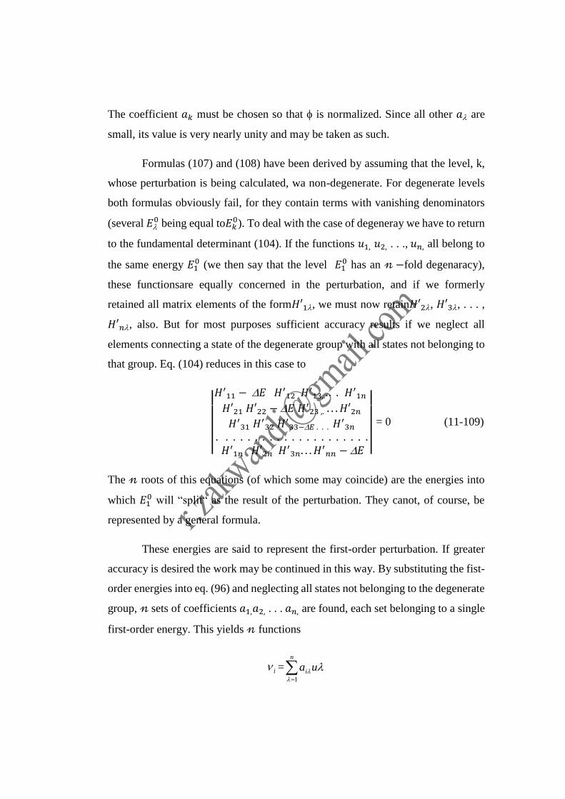
The coefficient 𝑎𝑘 must be chosen so that is normalized. Since all other 𝑎 are

small, its value is very nearly unity and may be taken as such.

Formulas (107) and (108) have been derived by assuming that the level, k,

whose perturbation is being calculated, wa non-degenerate. For degenerate levels

both formulas obviously fail, for they contain terms with vanishing denominators

(several 𝐸0 being equal to𝐸𝑘

0). To deal with the case of degeneray we have to return

to the fundamental determinant (104). If the functions 𝑢1, 𝑢2, . . ., 𝑢𝑛, all belong to

the same energy 𝐸10 (we then say that the level 𝐸1

0 has an 𝓃 −fold degenaracy),

these functionsare equally concerned in the perturbation, and if we formerly

retained all matrix elements of the form𝐻′1, we must now retain𝐻′2, 𝐻′3, . . . ,

𝐻′𝑛, also. But for most purposes sufficient accuracy results if we neglect all

elements connecting a state of the degenerate group with all states not belonging to

that group. Eq. (104) reduces in this case to

|

|

𝐻′11 − 𝐸 𝐻′12 𝐻

′13,.. . . 𝐻

′1𝑛

𝐻′21 𝐻′22 − 𝐸 𝐻′23 ,. . . . 𝐻′2𝑛𝐻′31 𝐻

′32 𝐻

′33−𝐸 . . . 𝐻

′3𝑛

. . . . . . . . . . . . . . . . . . . . . 𝐻′1𝑛 𝐻′2𝑛 𝐻

′3𝑛. . . 𝐻

′𝑛𝑛 − 𝐸

|

| = 0 (11-109)

The 𝓃 roots of this equations (of which some may coincide) are the energies into

which 𝐸10 will “split“ as the result of the perturbation. They canot, of course, be

represented by a general formula.

These energies are said to represent the first-order perturbation. If greater

accuracy is desired the work may be continued in this way. By substituting the fist-

order energies into eq. (96) and neglecting all states not belonging to the degenerate

group, 𝓃 sets of coefficients 𝑎1,𝑎2, . . . 𝑎𝑛, are found, each set belonging to a single

first-order energy. This yields 𝓃 functions

i =

uan

i1

If now we construct matrix elements with the 𝓋 −functions , dHvvH jiij ' , these

will be diagonal; for solving (109) is the well-known procedure for diagonalizing

the matrix H’. (See Chapter 10.) Hence, when the 𝒱 – functions are chosen to

represent the 𝓃 degenerate states, the second order perturbation can be computed

by formula (107), from which the terms with vanishing denominator sre now absent

because every 𝐻′𝑘 corresponding to them is zero.

11.23. Example : Non-Degenerate Case. The stark Effect.

Let 𝐻0 represent the Hamiltonian operator for anyone –electron system, and let

𝜓1,𝜓2, be its eigenfunctions. When a uniform electric field along X is applied, the

term H’ = eFx is added to 𝐻0, e being the electronic charge and F the field strength.

The normal state of the system is non-degenerate, hence formula (107) may be used.

Denoting the normal state by the subscript zero, we find

2

0

0

0

022

000 '

EE

xFeeFx (11-110)

Here 𝑥0𝜆 = 𝜓0𝑥𝜓𝜆d. The first term on the right is usually zero because|𝜓0|

2 is an

even function of 𝓍 ; thus the “ first-order Stark effect” is absent.

In classical physics, theincrement in energy of an atom due to a static

electric field is expressed in terms of the polarizability 𝒶 in the form

2

2

1aF

On comparing this with (110) we find for the polarizability of the normal

state of our system

∝= 2𝑒2∑|ᵪ0𝜆|

2

𝐸𝜆0−𝐸𝜆

0

𝜆

For an oscillator, this takes a particularly simple form, since all ᵪ0𝜆 vanish

with the exception of ᵪ01=√1/2𝛽 (cf. chapter 3, eqs. 92 and 93). Also, 𝐸𝜆0 =

(𝜆 +1

2) ℎ𝑣. Thus

∝= 2𝑒2𝑥012

ℎ𝑣

Comparison with the problem of sec. 21 shows that second-order perturbation

theory gives in this instance the same result as the variational method with the trial

function ∝0 𝜓0 +∝1 𝜓1 in general, however, the use of a simple variation function

yields a much poorer result for the polarizability than the method of sec. 22

11.24. Example: Degenerate Case. The Normal Zeeman Effect.

The energy states of the hydrogen atom were found to be

𝑅𝑛,𝑙(𝑟)𝑌𝑙(𝜃, 𝜑)

To a given 𝑙, there belong 2𝑙 + 1 spherical harmonics of the form

𝑌𝑙 = ∑ 𝑐𝑚

𝑙

𝑚=−1

𝑃𝑙𝑚(𝑐𝑜𝑠𝜃)𝑒𝑖𝑚𝜑 , (𝑃𝑙

−𝑚 = 𝑃𝑙𝑚

And each such combination with its own set of Coefficient,𝑐𝑚 Forms a proper

eignefunction when multiplied by𝑅𝑛,𝑙. The energy does not depend on m; the state

under consideration has therefore a 2𝑙 + 1 fold degeneracy.

Let us choose the 2𝑙 + 1 functions in the simplest possible way, namely by

letting each 𝑌𝑙 contain only one term, as follows:

𝑅𝑛,𝑙. 𝑐−𝑙𝑃𝑙𝑙𝑒−𝑖𝑙𝜑, 𝑅𝑛,𝑙. 𝑐−𝑙+1𝑃𝑙

𝑙−1𝑒−𝑖(𝑙−1)𝜑 , . . . . , 𝑅𝑛,𝑙. 𝑐1𝑃𝑙𝑙𝑒𝑖𝑙𝜑

And label them𝜙1, 𝜙2. . . , 𝜙2𝑙+1, in that order.

The Zeeman the splitting of the energy levels of an atom in a magnetic field.

When a uniform magnetic field along the Z-axis and of strength F is applied to the

hydrogen atom, its unperturbed Hamiltonian takes on the extra term.23

𝐻′ = − 𝑖ħ𝑒

2𝑀𝑐𝐹 𝜕

𝜕𝜑≡ −𝑖𝐴

𝜕

𝜕𝜑

Each matrix element 𝐻′ = ∫∅𝑖∗𝐻′dr contains the factor ∫𝑅𝑛,

2 𝑙𝑟2𝑑𝑟

Witch, by virtue of the normalization of the radial functions, is unity. If we

form, e.g. 𝐻12′ we obtain an integral over 𝜃 time∫ 𝑒𝑖𝑙𝜑

𝜕

𝜕𝜑 𝑒−𝑖(𝑙−1)𝜑𝑑𝜑

2𝜋

0, and this

vanishes in the same way all other non-diagonal matrix elements are seen to be zero.

The diagonal element 𝐻11′ is

−𝑖𝐴. (−𝑖𝑙).∫𝜙1∗𝜙1𝑑𝑟 = −𝐴𝑙

And the others are similarly constructed.

When these elements are substituted into (109) we have

|−𝑙𝐴 − ∆𝐸 0 0

0 −(𝑙 − 1)𝐴 − ∆𝐸 00 0 −(𝐿 − 2)𝐴 − ∆𝐸

000| = 0

………………………………………………………0

0 0 0…………… 𝑙𝐴 − ∆𝐸

The determinant is already diagonal, our choice of functions was a fortunate

one. The perturbed energies are clearly

23 See Vleeck, J.H., “The Theory of Electric and Magnetic Susceptibilities,” oxford,

1932. We write here M for the electron mass to avoid conflict with the summation

index m (magnetic quantum number). Note that H’ is the quantum representation

of 𝑒

2𝑀𝑐 F.L, where L is the angular momentum vector of sec. 11.3

∆𝐸 = 𝑚𝐴 = 𝑚ħ𝑒𝐹

2𝑀𝑐′𝑚 = −𝑙,−𝑙 + 1, . . . 0, 1. . . 𝑙

Classically, an electron in a magnetic field F performs a uniform precession of

angular frequency 𝜔𝐿 = 𝑒𝐹/2𝑀𝑐 known as the Larmor frequency. Thus we see

that ∆𝐸 = 𝑚ħ𝜔𝐿

Problem. Calculate the Stark effect of the rigid rotator (cf. sec. 11.12), for

the state 𝑙 = 3, adopting the same choice for the spherical harmonics as above.

Here 𝐻′ = 𝑒𝑎𝐹 𝑐𝑜𝑠 𝜃, provided the electric field F is along Z. the determinant will

not be diagonal. To calculate the matrix elements, use formulas (3-48 and 53).

Include in your calculation successively more states: 𝑙 = 2,3,4; 𝑙 = 1,2,3,4,5.

TIME-DEPENDET STATES. SCHRӦDINGER’S TIME EQUATION

11.25. General Considerations.

In all preceding considerations we have assumed that the states of the

systems in question were stationary ones, that the time coordinate could be

disregarded in describing them. In generalizing the theory so to make it applicable

to states which change in time it is well to look back and see why a time-free

description was possible thus far.

It is important to note that the time, t, in classical mechanics is canonically

conjugate to the energy, E, in the same sense that x is conjugate to 𝑝𝑥. Let us then

for the moment consider the operator 𝑝𝑥 = 𝑖ħ(𝜕

𝜕𝑥). Its eigenstates were seen to be

(cf. eq. 90 𝜓𝑝 = 𝑐𝑒(𝑖

ħ)𝑝𝑥

. What do they tell us about the distribution of the system

in x? The answer is, it is uniform.

Whatever is true at the point x1, is also true at the point x2. This is the

meaning of the uncertainty principle applied to the case at hand: if the momentum

is known with certainty, the state function is entirely noncommittal with regard to

x. If in the calculation of the mean value of an operator Q,

�� = ∫𝜓𝑝∗𝑄𝜓𝑝𝑑𝑟

Q did not depend on x, we could have afforded to neglect the factor 𝑒(𝑖

ℎ)𝑝𝑥

of

𝜓𝑝 altogether. It had to be included, however, because most operators of interest do

depend on x

But this trivial situation existed with regard to the time coordinate in all the

Schrodinger problems considered heretofore. The states were those in which the

energy was known with certainty, and for this reason the state functions were

completely indiscriminate in respect to t. What was true at t1 was also true at t2.

Moreover, the other operators used were independent of t. This condition will

always be present as long as we are dealing with closed systems, for the energy will

then be constant in time.

When the system is an open one, the present method must clearly fail. But

the last remarks contain the hint that we should, perhaps, associate with E the

operator --ih (𝜕/𝜕𝑡). This would lead to the eigenvalue equation.

−𝑖ℎ 𝜕

𝜕𝑡𝜓 = 𝐸𝜓

Which is certainly too simple because the energy depends on other things

beside the time. The example above gives us no definite lead at this point because

pa does possess the single dependence on x. There is, however, only one reasonable

way to include these other variables, namely, to put them into E, which thereby

ceases to be an eigenvalue: E must be replaced by the Hamiltonian operator H. We

then arrive at Schrodinger’s time equation

−𝑖ℎ 𝜕

𝜕𝑡𝜓 = 𝐻𝜓 (11-111)

H is to be constructed as before by replacement of every Cartesian

coordinate pi by −𝑖ℎ (𝜕 /𝜕 𝑞𝑖) and the dependence on t is to be introduced

explicitly.

It is immaterial, of course, whether we choose eq. (111) or its complex conjugate

equation. The latter choice has certain advantages and will here be made.

Furthermore, we shall use the symbol a (more or less generally) for time-dependent

state functions and thus record Schrodinger’ time equation in the form

𝑖ℎ𝜕𝑢 (𝑞1…𝑞𝑛𝑡)

𝜕𝑡= 𝐻 (−𝑖ℎ

𝜕

𝜕𝑞1, …− 𝑖ℎ

𝜕

𝜕𝑞𝑛; 𝑞1…𝑞𝑛; 𝑡) (𝑞1…𝑞𝑛; 𝑡) (11-112)

This equation, being of the first order in t, permits prediction of the state u at any

future (or past) time when u is known as a function of the coordinates at present.

Although it is closely related to the preceding deve10pments, eq. (112) is a new

postulate not derivable from those already given. The present theory must be valid

also in the special case when H does not contain t. When that is true eq. (112) is

separable. On writing 𝑢 = 𝜓(𝑞1 . . . 𝑞𝑛). 𝑓(𝑡)it becomes equivalent to the

equation.

𝐻ψ

𝜓=iℏ

𝜕𝑓𝜕𝑡

𝑓

Each side of which must represent a constant. But in View of the form of ~

the left-hand side, that constant must be one of the eigenvalues of the operator H,

say EA, so that

𝐻𝑒𝑛𝑐𝑒 𝜕𝑓

𝑎𝑡=−𝑖𝐸𝜆ℏ

𝑓

The general solution of eq. (112) for the special case in which H .is

independent of the time is

𝜐 = ∑ 𝑐𝜆 𝜆𝜓𝜆𝑒(0𝑖𝐸𝜆/ℏ)𝑡 (11-113)

We have formerly said that any state function, such as u, could be expanded

in the orthonormal system of functions 114.. This expansion was written as

𝜐 =∑𝑎

𝜆

𝜆𝜓𝜆

We now see that this is indeed true even when the analysis is made on the

basis of eq. (012), but the coefficients a) are always functions of the time: 𝑎𝜆 =

𝑐𝜆 – (𝑖𝐸𝜆ℎ)𝑡. The mean value of E, computed for the state

�� =∑|𝑐𝜆| 2𝐸𝜆 =∑|𝑎𝜆| 2𝐸𝜆𝜆𝜆

It is independent of t. But the probability of finding the system at the point

q1. . . qnof configuration space, u∗𝑢 = ∑ 𝑐𝜆∗

𝜆 𝑐𝜆𝝍𝜆∗𝝍𝝁𝒆

(𝒊

ħ)(𝐸𝜆−𝐸𝜇)𝑡

is a

superposition of oscillating functions of the time. The only way for this time

dependence to be obliterated would be to have 𝑐𝜆 = 𝛿𝜆 in which case.

𝑢 ∗ 𝑢 = 𝜓𝑗∗𝜓𝑗

Thus, whenever a state is formed by superposition of energy eigenstates, the

mean energy of the system remains constant, but the configuration of the system

changes in time. The reader should note, of course, that the solution of the

Schrodinger equation (12) when multiplied by 𝑒−(𝑖𝐸𝜆/ℎ)𝑡 is also a solution of (112),

but that the solution of (112) does not in general satisfy (12).

Problem. Let the time-dependent Hamiltonian be H = H o + V (t), where H0

acts only on space coordinates and has eigenfunctions 1h, eigenvalues Ex. Show

that

𝑢 =∑𝑐

𝜆

𝜆𝜓𝜆𝑒−(𝑖ℏ)(𝐸𝜆𝑡+∫𝑉𝑑𝑡

11.26. The Free Particle; Wave Packets.

The Eigenfunction of the energy of a free mass point (cf. sec. 11.9) moving

in one dimension without restriction are 𝜓𝑘 = 𝑒−𝑖𝑘𝑥 its energies𝑒𝑘 =ℎ2

2𝑚𝑘2, and

there is no quantization. The general solution of eq. (112) for the free particle is

therefore,

𝑢 = ∫ 𝑐(𝑘)∞

−∞𝑒𝑖[𝑘𝑥−(

ℎ2

2𝑚𝑘2𝑡]𝑑𝑘 (11-114)

A function constructed after the manner of (113) but with an integral instead

of a sum. An integral very similar to this has been already encountered in the

mathematical formulation of waves (cf. eq. 7-38) and of diffusion phenomena (eq.

7-53). It is interesting to inquire what form it will have at some time t if at t = 0 it

is given by 𝑢 = 𝑢0(𝑥). the coefficient 𝑐(𝑘) may be determined by Fourier analysis.

We have

𝑢0 = ∫ 𝑐(𝑘)𝑒𝑖𝑘𝑥𝑑𝑘∞

−∞

Whence by eq. 8-13

𝑐(𝑘) =1

2𝜋∫ 𝑢𝑜(𝜉)𝑒

−𝑖𝑘𝜉∞

−∞

𝑑𝜉

Eq. 114 therefore reads

𝑢(𝑥, 𝑡) =1

2𝜋∬ 𝑢𝑜(𝜉)𝑒

−𝑖[𝑘(𝑥−𝜉)−(ℎ/2𝑚)𝑘2𝑡]∞

−∞

𝑑𝜉𝑑𝑘

In this instance, the integration over to cannot be performed (as it could in

the diffusion problem, sec. 7.14). To proceed further it is necessary to introduce the

function 𝑢𝑜 explicitly.

Assume that 𝑢0 = 𝑒−𝑥2/2𝑎2. Then, with the use of the formula.

∫ 𝑒−𝜆𝑥2+𝑖𝜇𝑥𝑑𝑥 = √

𝜋

𝜆𝑒−𝜇

2/4𝜆∞

−∞ (11-115)

We find

𝑐(𝑘) =𝑎

√2𝜋𝑒−𝑎

2𝑘2/2

Hence

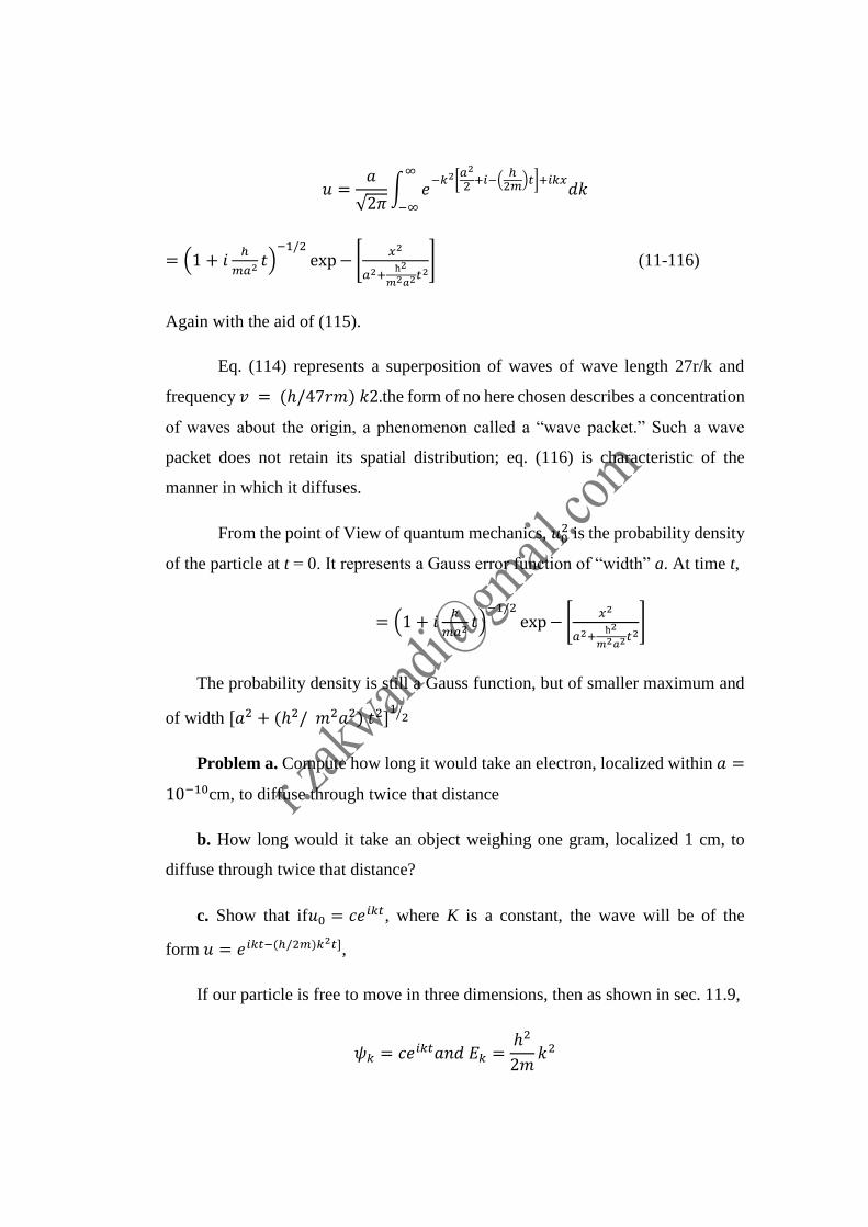
𝑢 =𝑎

√2𝜋∫ 𝑒

−𝑘2[𝑎2

2+𝑖−(

ℎ2𝑚

)𝑡]+𝑖𝑘𝑥𝑑𝑘

∞

−∞

= (1 + 𝑖ℎ

𝑚𝑎2𝑡)−1/2

exp− [𝑥2

𝑎2+ħ2

𝑚2𝑎2𝑡2] (11-116)

Again with the aid of (115).

Eq. (114) represents a superposition of waves of wave length 27r/k and

frequency 𝑣 = (ℎ/47𝑟𝑚) 𝑘2.the form of no here chosen describes a concentration

of waves about the origin, a phenomenon called a “wave packet.” Such a wave

packet does not retain its spatial distribution; eq. (116) is characteristic of the

manner in which it diffuses.

From the point of View of quantum mechanics, 𝑢02 is the probability density

of the particle at t = 0. It represents a Gauss error function of “width” a. At time t,

= (1 + 𝑖ℎ

𝑚𝑎2𝑡)−1/2

exp− [𝑥2

𝑎2+ħ2

𝑚2𝑎2𝑡2]

The probability density is still a Gauss function, but of smaller maximum and

of width [𝑎2 + (ℎ2/ 𝑚2𝑎2) 𝑡2]12⁄

Problem a. Compute how long it would take an electron, localized within 𝑎 =

10−10cm, to diffuse through twice that distance

b. How long would it take an object weighing one gram, localized 1 cm, to

diffuse through twice that distance?

c. Show that if𝑢0 = 𝑐𝑒𝑖𝑘𝑡, where K is a constant, the wave will be of the

form 𝑢 = 𝑒𝑖𝑘𝑡−(ℎ/2𝑚)𝑘2𝑡],

If our particle is free to move in three dimensions, then as shown in sec. 11.9,

𝜓𝑘 = 𝑐𝑒𝑖𝑘𝑡𝑎𝑛𝑑 𝐸𝑘 =ℎ2

2𝑚𝑘2

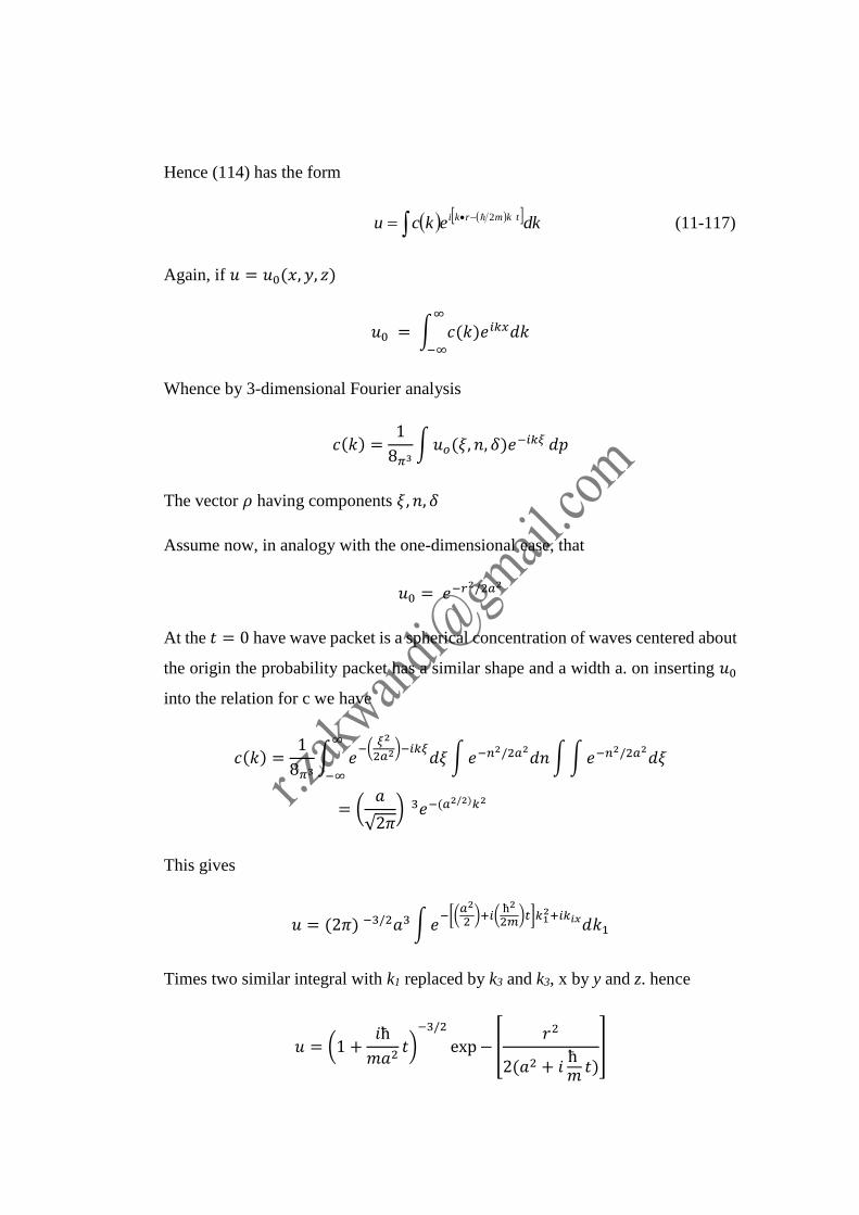
Hence (114) has the form

dkekcu tkmrki 2 (11-117)

Again, if 𝑢 = 𝑢0(𝑥, 𝑦, 𝑧)

𝑢0 = ∫ 𝑐(𝑘)𝑒𝑖𝑘𝑥𝑑𝑘∞

−∞

Whence by 3-dimensional Fourier analysis

𝑐(𝑘) =1

8𝜋3∫𝑢𝑜(𝜉, 𝑛, 𝛿)𝑒

−𝑖𝑘𝜉 𝑑𝑝

The vector 𝜌 having components 𝜉, 𝑛, 𝛿

Assume now, in analogy with the one-dimensional ease, that

𝑢0 = 𝑒−𝑟2/2𝑎2

At the 𝑡 = 0 have wave packet is a spherical concentration of waves centered about

the origin the probability packet has a similar shape and a width a. on inserting 𝑢0

into the relation for c we have

𝑐(𝑘) =1

8𝜋3∫ 𝑒

−(𝜉2

2𝑎2)−𝑖𝑘𝜉

𝑑𝜉∞

−∞

∫𝑒−𝑛2/2𝑎2𝑑𝑛∫∫𝑒−𝑛

2/2𝑎2𝑑𝜉

= (𝑎

√2𝜋) 3𝑒−(𝑎

2/2)𝑘2

This gives

𝑢 = (2𝜋) −3/2𝑎3∫𝑒−[(

𝑎2

2)+𝑖(

ħ2

2𝑚)𝑡]𝑘1

2+𝑖𝑘𝑖𝑥𝑑𝑘1

Times two similar integral with k1 replaced by k3 and k3, x by y and z. hence

𝑢 = (1 +𝑖ħ

𝑚𝑎2𝑡)−3/2

exp− [𝑟2

2(𝑎2 + 𝑖ħ

𝑚𝑡)]

The interpretation of this result is not different from that of (116).

Before leaving the subject of “particle waves” we should remark that every

component wave of the packet (117), being of the form 𝑒𝑖(𝑘.𝑟−2𝜋𝜈𝑡 travels in a

positive direction along k. Had we chosen the sign as in eq. (111) and not as in

(112), the waves would have been of the form 𝑒𝑖(𝑘.𝑟−2𝜋𝜈𝑡 which implies that they

travel along –k. Since 𝑘ħ represents the momentum of the particle, the latter choice

is a unusuitable one. We also also note that the wave length 𝜆 =2𝜋

𝑘=

2𝜋ħ

𝑚𝑤=

ℎ

𝑚𝑤

conforms to the De Broglie formula. The phase velocity of the waves is 𝑣𝜆 =ħ𝑘

2𝑚=

𝑚𝑤

2𝑚= 𝑣/2 but their group velocity24 defined as 2𝜋 (

𝑑𝑣

𝑑𝑘) = 𝑣 is equal to the classical

speed of the particle.25

11.27. Equation of Continuity, Current. If the state function changes in time in

accordance with the Schrӧdinger equation.

𝐻𝑢 = 𝑖ħ𝑢 (11-118)

Will it remain normalized? If it does not, there occurs a destruction or creation of

probability, while initially there was certainty, a situation which would clearly be

physically untenable. Permanence of normalization, however, follows immediately

from (118).

For

𝜕

𝜕𝑡∫𝑢 ∗ 𝑢𝑑𝜏 = ∫[𝑢 ∗ 𝑢 + 𝑢 ∗ 𝑢] 𝑑𝜏 =

𝑖

ħ ∫[𝑢𝐻 ∗ 𝑢 ∗ +𝑢 ∗ 𝐻𝑢] 𝑑𝜏

Because of (118) and the last expression is zero on account of the Hermitian

character of H.

24 For a discussion of group velocity, see Sommerfeld, “Wellenmechanischer

Erganzungsband “Friedr. Vieweg & Shon, Braunschweig, 1929, p.46. 25 This form of I is correct so long as the potential energy V is of the scalar form

here used. When H contains a vector potential, A, the term (e/c) A must be added

to the exspression for the current here given.

Having shown that 𝑢 ∗ 𝑢 is conserved we can define a probability current

by subjecting u*u, which we will 𝜌 for the moment, to the equation of continuity

𝜕

𝜕𝑡+ ∇. I = 0 (11-119)

Whatever I turns out to be must be regarded as the current corresponding to the

“flow” of the quantity u*u. we shall limit our consideration to the case of a single

particle so that

𝐻 =ħ2

2𝑚∇2 + 𝑉 (𝑥, 𝑦, 𝑧)

Althought generalization to many-deminsioned configuration space is easy.

Again because of (118)

𝜕𝑝

𝜕𝑡= 𝑢 ∗ 𝑢 + 𝑢 ∗ 𝑢 =

𝑖

ħ(𝑢𝐻 ∗ 𝑢 ∗ −𝑢 ∗ 𝐻𝑢)

=𝑖ħ

2𝑚(𝑢 ∗ ∇2𝑢 − 𝑢∇2𝑢 ∗) = ∇ [

𝑖ħ

2𝑚(𝑢 ∗ ∇ 𝑢 − 𝑢 ∇𝑢 ∗)]

To satisfy (119) we must put

𝐼 = −𝑖ħ

2𝑚(𝑢 ∗ ∇ 𝑢 − 𝑢∇ 𝑢 ∗) (11-120)

It is interesting to observr that a state u which has no complex devendence onn a

space variable has no current associated with it. Thus, in theFree particle problem,

𝑐𝑜𝑠 𝑘𝑥 and sin 𝑘𝑥 represent stationary states, but 𝑒𝑖𝑘𝑥 and 𝑒−𝑖𝑘𝑥 have currents.

Problem. Compute for the various regions of the barrier problems

considered in sec. 11.10

11.28. Application of Schrӧdinger’s Time Equation. Simple Radiation

Theory.

The cases in which eq. (118) can be solved exactly are not numerous and not very

interesting. When the time equation methods, the most useful of which will now be

illustrated.

Let an atom, whoose normal Hamiltonian function, free from all

perturbations, is 𝐻0, be suddenly subjected to a light wave which adds a perturbing

energy

𝑉(𝑥, 𝑡) = −𝑒𝐹0𝑥 sin𝜔𝑡 (11-121)

To H. Physically, this means the light wave is monochromatic and has

frequency 𝑣 = 𝜔/2𝜋; its electric is along X and of amplitude 𝐹0 if V did not contain

x and sin𝜔𝑡 in product form, eq. (118) with 𝐻 = 𝐻0 + 𝑉 would be separable; the

fusion of x and t into V spoils separability.

In solving (118) we use the following initial condition: At𝑡 = 0, when the

atom was exposed to the perturbation V, the atom was certainly in an eigenstate of

the operator𝐻0, say in the state 𝜓1 corresponding to the energy 𝐸1 which we shall

take to be the lowest energy of the system. Or, if we wish to include the trivial time

dependence of the state, we take

𝑢 = 𝜓1𝑒−(𝑖𝐸1/ħ)𝑡 (11-122)

The solution of

(𝐻0 + 𝑉)𝑣 = 𝑖ħ𝑣 (11-123)

Which we desire, is certainly available in the form

𝑣 = ∑ 𝑐𝜆𝜓𝜆𝑒−(𝑖𝐸1/ħ)𝑡𝜆 (11-124)

26 Imples that the wave length of the light is large compared with the size of the

atom. Correctly 𝑉 = −𝑒𝐹0𝑥 sin (𝜔𝑡 −2𝜋𝑧

𝜆), and we are omitting the term𝑧/𝜆. The

legitimacy of this will be clear form the following analysis.

Provided we let the coefficients 𝑐 be functions of the time. This follows

immediately from the completeness of the 𝜓𝜆 with respect to function of the space

coordinates. When (124) is substituted into (123). There results

∑𝑐𝜆

𝜆

(𝐻0 𝜓𝜆 + 𝑉 𝜓𝜆)𝑒−(𝑖𝐸1/ħ)𝑡 =∑(𝑐𝜆𝐸𝜆 𝜓𝜆 + 𝑖ħ𝑐𝜆 𝜓𝜆)𝑒−(𝑖𝐸1/ħ)𝑡𝜆

Wherein each term 𝐻0 𝜓𝜆 on the left cancels 𝐸𝜆 𝜓𝜆 on the right. Let us now

multiply the remaining terms of the equation by 𝜓𝑘∗ and integrate over configuration

space, remembering the orthogonality of the 𝜓𝜆. Then after simple rearrangement,

𝑐𝑘 = −𝑖

ħ∑ 𝑐𝑘𝑉𝑘𝜆𝜆 𝑒𝑖[

𝐸𝑘−𝐸𝜆ħ

]𝑡, 𝑘 = 1,2,3, .. . (11-125)

Where, as usual,

𝑉𝑘𝜆 = ∫𝜓𝑘∗ 𝑉 𝜓𝜆𝑑𝑟

If the unperturbed atom has an infinite number of states, (125) represents an

infinite set of linear differential equations, which in general can’t be solved. But we

nw recall that 𝑡 = 0 𝑣 = 𝑢 which means that all 𝑐𝑘 except 𝑐1 were zero at that time.

There after 𝑐1 decayed from 1 to some smaller value, while all other c’s grew from

0 to various finite values. We now limit our inquiry to times so small that 𝑐1 is still

sensibly unity, and the other c’s are small compared with it, although 𝑐1 may be

quite comparable with the time derivatives of other c’s. This permits the

26 Eq. (121) is a valid approximation for the purpose at hand. It neglects the energy

due to the magnetic vector of the light wave whose contribution is small compared

to (121) in the ratio 𝑣/𝑐, where 𝑣 is the velocity of the charge composing the atom

and 𝑐 the velocity of light. For hydrogen 𝑣/𝑐, is 1/137. Furthermore, eq. (121)

approximation of replacing every 𝑐𝜆 on the right-hand side of (125) by its value at

𝑡 = 0 while retaining every 𝑐𝑘. The equation then beomes

𝑐𝑘 = −𝑖

ħ𝑉𝑘1𝑒

(𝑖ħ)(𝐸𝑘−𝐸1)𝑡

To simplify writing we introduce the abbreviation

(𝐸𝑘 − 𝐸1)

ħ≡ 𝜔𝑘

And observe that ever 𝜔𝑘 > 0, since, as we are assuming, 𝐸1 is the lowest

energy state. In view of (121),

𝑉𝑘1 = −𝑒𝐹0𝑥𝑘1 sin𝜔𝑘 =1

2𝑖𝑒𝐹0𝑥𝑘1(𝑒

𝑖𝜔𝑡 − 𝑒𝑖𝜔𝑡)

So that

𝑐𝑘 =𝑒𝐹02ħ

𝑥𝑘1[𝑒𝑖(𝜔𝑘+𝜔)𝑡 − 𝑒𝑖(𝜔𝑘−𝜔)𝑡]

On integration,

𝑐𝑘 =𝑖𝑒𝐹02ħ

𝑥𝑘1 [𝑒𝑖(𝜔𝑘−𝜔)𝑡 − 1

𝜔𝑘 − 𝜔−𝑒𝑖(𝜔𝑘+𝜔)𝑡 − 1

𝜔𝑘 + 𝜔] , 𝑘 ≠ 1

Where we have at once adjusted the constant of integration so that 𝑐𝑘 = 0

when 𝑡 = 0. For physical reasons, only the first term in the square parenthesis need

be retained because it alone can attain appreciable magnitude. (Both 𝜔 and 𝜔𝑘 > 0

). In fact 𝑐𝑘 is large only when 𝜔 ≈ 𝜔𝑘 and this fact is accentuated when 𝑐𝑘 is

squared:

|𝑐𝑘|2 =

𝑒2𝐹02

2ħ2|𝑥𝑘1|

21 − cos(𝜔𝑘 − 𝜔)𝑡

(𝜔𝑘 − 𝜔)2=𝑒2𝐹0

2

4ħ2|𝑥𝑘1|

2 𝑠𝑖𝑛2[

(𝜔𝑘 − 𝜔)2 𝑡]

((𝜔𝑘 −𝜔)

2 𝑡)2

We now interpret this result. The coefficient 𝑐𝑘 is, in view of (124), the 𝑘 −

𝑡ℎ probability amplitude in the expansion of the state function 𝑣 at time 𝑡 in terms

of energy eigenstates of the normal atom. Hence because of sec. 5 |𝑐𝑘|2 is the

probability at time 𝑡 the 𝑘 − 𝑡ℎ energy level of the atom be excited; it is the

“transition probability” from state 1 to state 𝑘 when the atom has been exposed to

monochromatic light of frequency 𝜔/2𝜋 fot 𝑡 seconds.

Many interesting conclusions of a physical nature can be drawn from eq.

(126), of which only two will here be mentioned. First, the transition probability is

proportional to the square of the matrix element connecting the states in question.

Whenever 𝑥𝑘1 is the criterion of a “forbidden” transition in the second place, the

transition probability is small unless𝜔 ≈ 𝜔𝑘, which is the Bohr frequency

condition.

Problem. The reader may be surprised to find that |𝑐𝑘|2 is not a linier

function of𝑡, as might be except on physical grounds. Show that, when the incident

light forms a continuous spectrum of uniform intensity, |𝑐𝑘|2 is the proportional

to 𝑡. (For this purpose, (126) must be ntegrated over 𝜔 from 0 to ∞; but the

integration may without appreciable error be taken from −∞ 𝑡𝑜 + ∞)

ELECTRON SPIN. PAULI THEORY

11.29. Fundamentals of the Theory.

The theory so far developed describes the general behavior of atomic and molecular

systems surprisingly well, but it makes some false predictions, particularly with

regard to the finer details of the energy states of atoms, the Zeeman Effect and the

magnetic properties of electrons. It was soon apparent that the state of a single

electron could not be represented as a function of three space coordinates alone, but

that another parameter was required whose interpretation was for some time in

doubt. Most decisive in clarifiying the situation was the spectroscopic observation

of the doubling of the energy levels of a single electron: in all alkali atoms, for

instance, two levels are found where the Schrӧdinger equation permits only one.

The energy difference between these levels was such as would be produced by a

small magnet of magnetic field present in the atom on account of the these two

energy states was known to be different it was equal to that caused by the electron’s

orbital motion, plus ħ/2 in the other state.

Uhlenbeck and Goudsmit suggested that the electron behaves like a

spinning top having a “spin” angular momentum of magnitude ħ/2 which

however, can only add or subtract its whole amount, in quantum fashion, to any

angular momentum the electron already prossesses as a result of its orbital motion.

Correspondingly, the electron generates by its spin a magnetic moment of

magnitude ħ𝑒/2𝑚𝑐 (𝑚 is the electron mass, 𝑐 the velocity of light), and this also

communicates itself in 𝑡0 𝑡0 , either parallel or in opposition, to any magnetic

moment already present.

To describe the electron spin as an angular momentum of the usual kind and

to associate with it an operator like L (eq.44) proved a fruitless undertaking, chiefly

because L would have more than two eigentatates. The most successful procedure

of including the spin in the quantum mechanical formalism, aside from Dirac’s

relativistic treatment of the electron, is that of Pauli which will now be describe.

What follows will refer only to the spin states of a single electron some applications

to several electrons may be found in sec. 34 and 35.

Since the three space coordinates are insufficient to specity the complete

state of an electron, we introduce a fourth, the “spin coordinates” and denote it

by 𝑠𝑧. It corresponds, in classical language to the cosine of the angle between the

axis of the spin angular momentum and the Z-axis of coordinates. This visual

interpretation while in no way dictated by the mathematical formalism, will be

found a useful mental aid. Thus the state function of an electron has the form.

𝜙(𝑥, 𝑦, 𝑧, 𝑠𝑧)

Since in all that follows, the hypothetical spin coordinates 𝑠𝑧 and 𝑠𝑦. Are

never needed, we shall hence forth delete the subscript 𝑧 on 𝑠 but retain the above

interpretation. Hence 𝜙 = 𝜙(𝑥, 𝑦, 𝑧, 𝑠𝑧). Finally, it is well for the moment to

abstract attention entirely from the space dependent part of the wave function, i.e.,

to consider 𝑥, 𝑦, 𝑧 as fixed, cocentraining our inquiry solely upon the electron spin.

Then 𝜙 = 𝜙(𝑠)

If s, like x, y and z, were permitted to assume a continuous range of values,

difficulties would result. Pauli therefore postulates-in a manner admittedly ad hoc

and designed to force success of the theory-that the range of 8 consists of only two

points: s = ±11 (classical meaning: spin vector is parallel or in opposition to Z). A

function of s is therefore defined only at these two points. The most general spin

function is, accordingly.

∅(𝑠) = 𝑎𝛿𝑠+1 + 𝑏𝛿𝑠−1 (11-127)

Where the 𝛿′s are Kronecker symbols. Our postulates involved certain

integrals over configuration space. But an integral over configuration space

consisting of two points vanishes. It becomes necessary to redefine the integral as

a summation over the two points:

∫𝐹(𝑠)𝑑𝑠 ≡ 𝐹(−1) + 𝑓(1)

If ∅(𝑠) is to be normalized

∫(|𝑎| 2𝛿𝜏+1𝜏 +(𝑎∗𝑏 + 𝑏∗𝑎)𝛿𝑠 + 𝛿𝑠−)𝑑𝑠 = |𝑎| 2 + 𝑏| 2 = 1| (11-128)

In a very trivial sense, eq. (127) represents an expansion of a function (Ms) in a

complete orthonormal set of functions𝛿𝑠+1 𝑎𝑛𝑑 𝛿𝑠−1. To what operator do these

two functions belong as eigenstates? The answer is suggested by intuition and will

be justified by its complete success; it is the operator𝑠𝑧, which is associated with

the observable: spin angular momentum along Z. We must now give thought to the

mathematical structure of this operator.

Empirical evidence cited in the introductory paragraphs demands that its

two eigenvalues be ±h/2. Hence it must satisfy the two equations

𝑠2𝛿𝑠+1 =ℎ

2𝛿𝑠 + 1

𝑠2𝛿𝑠−1 =ℎ

2𝛿𝑠 − 1 (11-129)

It is possible to show that no differential operator of the type encountered previously

can satisfy these equations without giving rise to an infinite number of other

eigenstates. But why search for the operator? The simplest point of View, and that

here taken, is to regard eqs. (129) as a definition ofthe operator Sz

To simplify the notation, and to be in accord with custom, we now intro» duce the

symbol a(s) for𝛿𝑠+1, and𝛽𝑠−1. Furthermore, we define a new operator.

𝜎𝑧 =2

ℎ𝑠𝑧

Which has eigenvalues ±1, for the simple expedient to save writing. Then, in view

of (129),

𝛿𝑧𝑎(𝑠) = 𝑎(𝑠), 𝛿 𝑧𝛽(𝑠) = 𝛽(𝑠),

It is indeed possible and often useful to find an explicit operator in form of a matrix

which will satisfy these equations. This matrix is easily formed by means of the

principles outlined in sec. 17. Our eigenstates are 𝜓1 = 𝑎,𝜓2 = 𝛽, and we construct

(𝛿𝑧)𝑖𝑗 = ∫𝜓𝑖∗𝜎𝑧𝜓𝑗𝑑𝑟 with the integral replaced by a summation. We thus obtain

the two-square matrix

𝜎𝑧 = (1 0

0 − 1)

To let it operate on what was formerly the function (15(3) the latter has to be

regarded as a vector whose components are its expansion coefiicients:

If the function Q) is given by 𝜙(𝑠) = 𝑎𝑎 + 𝑏𝛽 a and b being numbers, then the

vector 𝜙(s) is

𝜙 = (𝑎

𝑏)

Thus, in the matrix representation,

𝜎𝑧𝜙 = (1 00−1)(𝑎𝑏)

And the reader will easily verify by the rules of Chapter 10 that the two 0

eigenvectors of 𝜎𝑧are 𝜙 = (𝑎0)𝑎𝑛𝑑 𝜙 =(0

𝑏)where the values of both a27And b must

be unity because of (128). The eigenvalues are, respectively, +1 and -1. But the

functions qt corresponding to the vectors (10) and (0

1) are clearly𝑎 𝑎𝑛𝑑 𝛽, which

takes us back to the scheme (130).

It is seen that there is a complete isomorphism between the two descriptions

of the operator SZ and its eigenstates 𝜙: One in terms of matrices and

eigenvectorsf‘where the rule of operations is (132); the other in terms of linear

substitution operators and eigenfunctions, Where the rule of operations is (130).

The question now arises as to the structure of the operators Sx and Sy,

associated with the other two components of the spin.28In endeavoring to construct

them it is important to recall one significant fact concerning the ordinary angular

momentum L: its components do not commute With one another. In fact (see eq. 7)

LzLy -LyLx = ihLz, LyLz -LzLy = ihLz

LzLx LxLz = ihLy

Let us assume that the components of the spin S, this being an angular momentum

operator, must be subject to the same commutation rules. In terms of a" rather than

S, we postulate

𝜎𝑧 𝜎𝑦 − 𝜎𝑦 𝜎𝑧 = 2𝑖𝜎𝑧; 𝜎𝑧 𝜎𝑦 − 2𝑖𝜎𝑥; 𝜎𝑧 𝜎𝑥 − 𝜎𝑥 𝜎𝑧 = 2𝑖𝜎𝑦

27 An operator p is in general uniquely determined when the result of is action upon

each member of an orthonormal set of function is known. The method of defining

an operator is ordinarily not useful because an infinite number of relation like (129)

would be required.

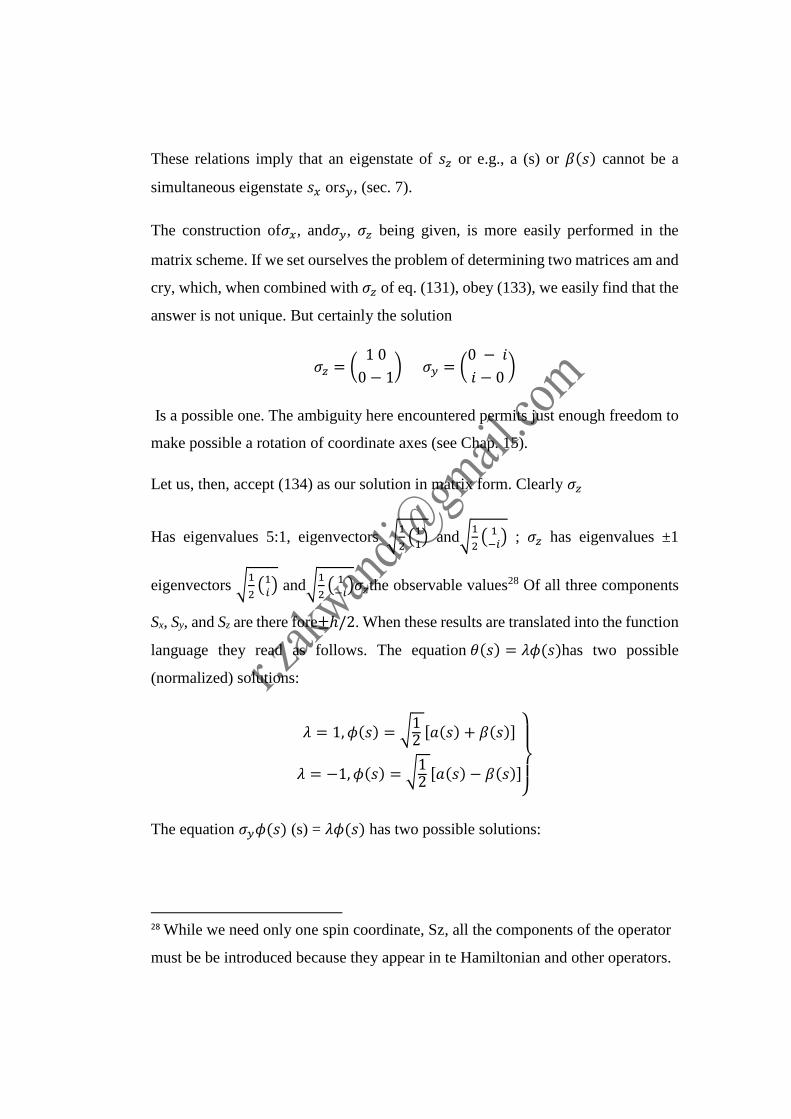
These relations imply that an eigenstate of 𝑠𝑧 or e.g., a (s) or 𝛽(𝑠) cannot be a

simultaneous eigenstate 𝑠𝑥 or𝑠𝑦, (sec. 7).

The construction of𝜎𝑥, and𝜎𝑦, 𝜎𝑧 being given, is more easily performed in the

matrix scheme. If we set ourselves the problem of determining two matrices am and

cry, which, when combined with 𝜎𝑧 of eq. (131), obey (133), we easily find that the

answer is not unique. But certainly the solution

𝜎𝑧 = (1 0

0 − 1) 𝜎𝑦 = (

0 − 𝑖

𝑖 − 0)

Is a possible one. The ambiguity here encountered permits just enough freedom to

make possible a rotation of coordinate axes (see Chap. 15).

Let us, then, accept (134) as our solution in matrix form. Clearly 𝜎𝑧

Has eigenvalues 5:1, eigenvectors √1

2(11) and√

1

2( 1−𝑖) ; 𝜎𝑧 has eigenvalues ±1

eigenvectors √1

2(1𝑖) and√

1

2( 1−𝑖)𝜎𝑧the observable values28 Of all three components

Sx, Sy, and Sz are there fore±ℎ/2. When these results are translated into the function

language they read as follows. The equation 𝜃(𝑠) = 𝜆𝜙(𝑠)has two possible

(normalized) solutions:

𝜆 = 1, 𝜙(𝑠) = √12 [𝑎(𝑠) + 𝛽(𝑠)]

𝜆 = −1, 𝜙(𝑠) = √12 [𝑎(𝑠) − 𝛽(𝑠)]

}

The equation 𝜎𝑦𝜙(𝑠) (s) = 𝜆𝜙(𝑠) has two possible solutions:

28 While we need only one spin coordinate, Sz, all the components of the operator

must be be introduced because they appear in te Hamiltonian and other operators.

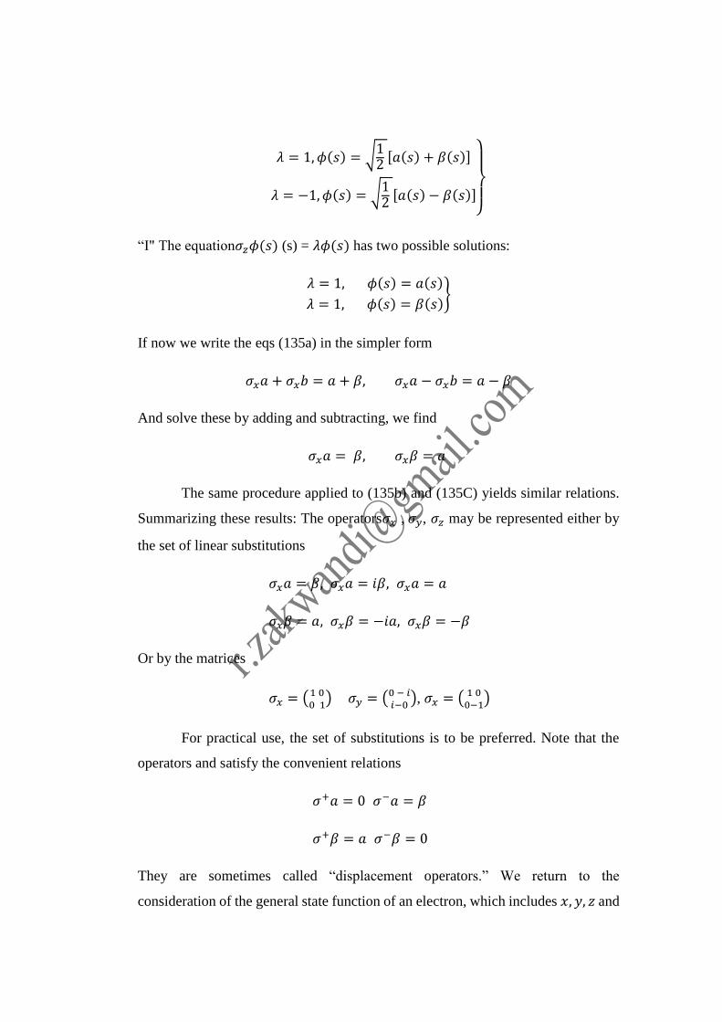
𝜆 = 1, 𝜙(𝑠) = √12 [𝑎(𝑠) + 𝛽(𝑠)]

𝜆 = −1, 𝜙(𝑠) = √12 [𝑎(𝑠) − 𝛽(𝑠)]

}

“I" The equation𝜎𝑧𝜙(𝑠) (s) = 𝜆𝜙(𝑠) has two possible solutions:

𝜆 = 1, 𝜙(𝑠) = 𝑎(𝑠)

𝜆 = 1, 𝜙(𝑠) = 𝛽(𝑠)}

If now we write the eqs (135a) in the simpler form

𝜎𝑥𝑎 + 𝜎𝑥𝑏 = 𝑎 + 𝛽, 𝜎𝑥𝑎 − 𝜎𝑥𝑏 = 𝑎 − 𝛽

And solve these by adding and subtracting, we find

𝜎𝑥𝑎 = 𝛽, 𝜎𝑥𝛽 = 𝑎

The same procedure applied to (135b) and (135C) yields similar relations.

Summarizing these results: The operators𝜎𝑥 , 𝜎𝑦, 𝜎𝑧 may be represented either by

the set of linear substitutions

𝜎𝑥𝑎 = 𝛽, 𝜎𝑥𝑎 = 𝑖𝛽, 𝜎𝑥𝑎 = 𝑎

𝜎𝑥𝛽 = 𝑎, 𝜎𝑥𝛽 = −𝑖𝑎, 𝜎𝑥𝛽 = −𝛽

Or by the matrices

𝜎𝑥 = (1 00 1) 𝜎𝑦 = (0 − 𝑖

𝑖−0), 𝜎𝑥 = (

1 00−1)

For practical use, the set of substitutions is to be preferred. Note that the

operators and satisfy the convenient relations

𝜎+𝑎 = 0 𝜎−𝑎 = 𝛽

𝜎+𝛽 = 𝑎 𝜎−𝛽 = 0

They are sometimes called “displacement operators.” We return to the

consideration of the general state function of an electron, which includes 𝑥, 𝑦, 𝑧 and

s as argument. Such a function may certainly be expanded in eigenfunctions of 𝜎𝑧

i.e

𝜙(𝑥, 𝑦, 𝑧, 𝑠) = 𝜙 + (𝑥, 𝑦, 𝑧)𝑎(𝑠) + 𝜙 − (𝑥, 𝑦, 𝑧)𝛽(𝑠)

Normalization now requires

∫𝜙∗𝜙𝑑𝑟 ≡∑𝜙∗𝜙𝑑𝑥𝑑𝑦𝑑𝑧

𝑠

= ∫(𝜙+∗ 𝜙+ + 𝜙−

∗𝜙−) 𝑑𝑥𝑑𝑦𝑑𝑧 = 1

The operators 𝜎𝑥𝜎𝑦𝜎𝑧 do not act on 𝜙+and 𝜙−which are only. Function of 𝑥, 𝑦, 𝑧

in other words, they commute with space coordinates. Thus, for instance

𝜎𝑦𝜙(𝑥, 𝑦, 𝑧, 𝑠) = 𝜎𝑦𝜙+𝑎 + 𝜎𝑦𝜙−𝛽 = 𝜙+𝜎𝑦𝑎 + 𝜙−𝜎𝑦𝛽 = 𝑖𝜙+𝛽 − 𝑖𝜙−𝑎

In the matrix scheme, 𝜙(𝑥, 𝑦, 𝑧, 𝑠) is represented by the vector

𝜙 = (𝜙+(𝑥, 𝑦, 𝑧, 𝑠)

𝜙−(𝑥, 𝑦, 𝑧, 𝑠))

In the sense of this analysis it may be said that the introduction of the spin in the

Pauli manner causes all Schrӧdinger function to become two-component functions.

Problem. Carry out the algebra involved in finding the two

Hermitian matrix (134).

11.30. Applications.

Atom in a Magnetic Field. Our interest here is not in a complete solution of this

problem, which may be found worked out in most books on quantum mechanics,

but in its silent mathematics features. We wish to find the energies of an electron

atom (e.g., hydrogen or, with good approximation, the alkalis) when it is placed in

a uniform magnetic field. The Hamiltonian consist of two parts, one acting on the

electrons space coordinates and one acting on the spin coordinate. The former will

be called 𝐻0 the letter is the “spin energy”. If the magnetics field Ἧ is taken along

the Z-axis, the classical energy of a particle of magnetic moment 𝜇 would be𝜇.Ἧ =

𝜇𝑧.Ἧ𝑧. But empiricalt, the magnetic moment associated with the spin is (ħ𝑒/2𝑚𝑐)𝜎

. We shall here write 𝜇 for the constantħ𝑒/2𝑚𝑐. In quantum mechanical

transcription, then, the “spin energy” is 𝜇Ἧ𝑧𝜎𝑧 where 𝜎𝑧 is interpreted as the

operator (130) or (131)

(𝐻0 + 𝜇Ἧ𝑧𝜎𝑧)Ѱ = 𝑬Ѱ 11-138)

Let

Ѱ(x, 𝑦, 𝑧, 𝑠) = 𝝍 + (x, 𝑦, 𝑧)𝛼(𝑠) + 𝝍 − (x, 𝑦, 𝑧)𝛽(𝑠)

And substitute obtaining

𝛼(s)[𝐻0 + 𝜇Ἧ𝑧 − 𝐸]𝜓+ + 𝛽(𝑠)[(s)[𝐻0 + 𝜇Ἧ𝑧 − 𝐸]𝜓− = 0

Provided relations (136) are used. Since ∝ 𝑎𝑛𝑑 𝛽 are linearly independent,

orthogonal functions of s, their coefficients in the las equation must separately

vanish. Hence we have

𝐻0𝜓+ + 𝜇Ἧ𝑧 = (𝐸 − 𝜇Ἧ𝑧)𝜓+ 𝐻0𝜓− + 𝜇Ἧ𝑧 = (𝐸 + 𝜇Ἧ𝑧)𝜓−

Now let 𝐸0 be an eigenvalue of 𝐻0 ψ0 the corresponding eigenfunction. The first

of eqs., (139) (which is nothing more than an eigenvalue equation for the

operator𝐻0) then says 𝑬 − 𝜇Ἧ𝑧 = 𝐸0 or𝐸 = 𝐸0 + 𝜇Ἧ𝑧𝜓+ = ψ0. On substituting

this value of E into the second equation it reads 𝐻0𝜓−=(𝐸0 + 2𝜇Ἧ𝑧)𝜓− and this

can only be satisfied by putting ψ− = 0 because (𝐸0 + 2𝜇Ἧ𝑧) is not an eigenvalue

of𝐻0. Thus we obtain as one solution of (138)

𝐸 = 𝐸0 + 𝜇Ἧ𝑧 Ѱ = 𝜓0(x, 𝑦, 𝑧) ∝ (𝑠) (11-140a)

But we can also start with the second of eqs. (139) and assume 𝜓−to be 𝜓0 𝐸 +

𝜇Ἧ𝑧to be 𝐸0 . Then 𝜓+ = 0 and we have

𝐸 = 𝐸0 − 𝜇Ἧ𝑧 Ѱ = 𝜓0(x, 𝑦, 𝑧)𝛽(𝑠) (11-140b)

How does the inclusion of the spin modify the eigenvalues and eigenfunction of the

Schrӧdinger equation when there is no magnetics field? The answer is obtained by

letting Ἧ𝑧 vanish in (140b). Both values of E coalesce to 𝐸0 which now represent

the ordinary Schrӧdinger energy in the absence of a field, but the functions Ѱ

remain distinct. The spin thus introduces a degeneracy into the Schrӧdinger

representation of states. Formulas (140) account- in a primitive way-for the

doubling of the alkali energy levels, the field Ἧ𝑧 being caused in that case by the

electron’s orbital motion, and not by external agencies.

Problem. Solve eq. (138) by the method of separation of variables, i.e., by

putting Ѱ = 𝜓(x, 𝑦, 𝑧)𝜙(𝑠) and show that (140) is the solution obtained by that

method also.

b. A Spin Problem. Having shown how spin and coordinate functions cooperate in

the description of the states of an electron, let us omit further reference to space

coordinates and inquire. What are the energies which an electron, placed in a

uniform magnetic field of arbitrary direction, may assume regardless of its

translational motion. The only energy of interest is that due to the sin. Let Ἧ be

the magnetics field strength. The Schrӧdinger equation reads.

𝜇Ἧ. 𝜎𝜓 = 𝜇(Ἧ𝑥𝜎𝑥 +Ἧ𝑦𝜎𝑦 +Ἧ𝑧𝜎𝑧)ψ(s) (11-141)

If Ἧ is taken along Z, the equation reduces to

𝜇Ἧ𝜎𝑧 . ψ(s) = 𝐸ψ(s) (11-142)

29

29 This can be seen explicitly if the equation is multiplied by either 𝛼(𝑠) or 𝛽(𝑠)

and the “integrated” over.

The operator on the left is but a constant multiple of oz and must therefore

have the same eigenfunctions as𝜎𝑧, i.e 𝑎 𝑎𝑛𝑑 𝛽. The corresponding eigenvalues are

at once seen to be E = ±𝜇ℋ. We shall show that eq. (141) has the same eigenvalues,

but different eigenfunctions. Make the substitution 𝜓 = 𝑎𝛼 − 𝑏𝛽(𝑠) in eq. (141).

On using, subsequently, relations (136) the result will be ‘𝑚𝑒𝑒𝑡: 4 + 𝑏𝑒 −

𝑛𝑒𝑤 𝑏𝑎) + 3€𝑧 < 𝑎𝑎 𝑏𝑒} − 𝐸𝑚𝑎 + 𝑤) = 0

𝜇{ℋ𝑧(𝑎𝛽 + 𝑏𝑎) − 𝑖ℋ𝑦(𝑎𝛽 − 𝑏𝑎) +ℋ𝑧(𝑎𝑎 + 𝑏𝛽)} − 𝐸(𝑎𝑎 + 𝑏𝛽) = 0

As before, the coefficients of a and 6 may be put equal to zero separately, so that

𝜇(ℋ𝑥𝑎 − 𝑖ℋ𝑦𝑎 −ℋ𝑧𝑏 = 𝐸𝑏

𝜇(ℋ𝑥𝑏 − 𝑖ℋ𝑦𝑏 −ℋ𝑧𝑎 = 𝐸𝑎}

If the equations are to have solutions a, b, which are different from zero, the

determinant of the coefficients of a, b must vanish, whence E = ±𝜇ℋ

On substituting E = +𝜇ℋ into the first of eqs. (143) and then taking the square of

its absolute value, we have

(ℋ𝑥2 +ℋ𝑦

2)|𝑎| 2 = (ℋ +ℋ𝑧) 2|𝑎| 2

Let us call the angle between ℋ and .the Z-axis,𝜃, so that 2(ℋ𝑥2 +ℋ

2 =

ℋ 2 𝑠𝑖𝑛 2 𝜃 and ℋ𝑧 = ℋ

𝑐𝑜𝑠 2 𝜃 . Furthermore, in View of (128), |𝑏| 2 = 1-

|𝑎| 2 . When these substitutions are made and the last equation is solved, the squares

of the absolute values of a, b are found to be 𝑐𝑜𝑠 2 𝜃/2 and𝑠𝑖𝑛 2 𝜃/2, respectively.

Let us then puta = cos𝜃/2, b = 𝑒𝑖𝛿sin 𝛿/2, treating 𝛿 as a phase constant. With

the further substitutions ℋ𝑧 = 𝐻 𝑠𝑖𝑛 𝜃 cos𝜙, ℋ𝑦 = 𝐻 sin 𝜃 𝑠𝑖𝑛 𝜙 where 𝜙 is the

azimuth of the field, we find from (143) that 𝜎 = −𝜙

In a similar way, when 𝐸 = −𝜇𝐻, 𝛿 = 𝜋 − 𝜙, 𝑎 =𝑠𝑖𝑛𝜃

2𝑏 = −𝑒−𝑖𝜙

𝑐𝑜𝑠𝜃

2

We conclude that eq. (141) has the eigenvalues 𝐸1 = 𝜇𝐻, 𝐸2 = −𝜇ℋ and the

corresponding eigenfunctions

𝜓1 = cos𝜃

2. 𝑎(𝑠) + sin

𝜃

2𝑒−𝑖𝜙 𝛽(𝑠)

𝜓2 = sin𝜃

2. 𝑎(𝑠) + cos

𝜃

2𝑒−𝑖𝜙 𝛽(𝑠)

} (11-143)

Notice that, when the field ℋ is the reversed in direction (i.e 𝜃 → 𝜋 − 𝜃, 𝜙 → 𝜙 +

𝜋), and 𝜓1 and 𝜓2 exchange their roles.

Problem. Solve eq. (141) by diagonalizing the matrix ℋ𝑧𝜎𝑧 +ℋ𝑧𝜎𝑧 +

ℋ𝑧𝜎𝑍 = (ℋ𝑧

ℋ𝑧 + 𝑖ℋ𝑦

ℋ𝑧 − 𝑖ℋ𝑦

−𝑖ℋ𝑧) and show that it leads to the same result.

THE MANY-BODY PROBLEM AND THE EXCLUSION PRINCIPLE

11.31. Separation of the Coordinates of the Center of Mass.

In classical mechanies, a system containing many particles and subject only to

internal forces behaves in such a way that its center of mass moves uniformly on a

straight line. As a corollary of this theorem every classical two-body problem may

be reduced to a one-body problem.30A similar fact may be proved in quantum

theory.

The Schrӧdinger equation for a system of n particles of masses 𝑚1. . . 𝑚2

reads:

(−∑ħ2

2𝑚𝑖

𝑛𝑖 ∇1

2 + 𝑉)𝜓 = 𝐸𝜓 (11-145)

Where ∇12=

𝜕2

𝜕𝑥𝑖2 +

𝜕2

𝜕𝑦𝑖2 +

𝜕2

𝜕𝑧𝑖2 the potensial energy, V, is to be regarded as a function

of the relative coordinates 𝑥𝑗 − 𝑥𝑖, 𝑦𝑗 − 𝑦𝑗 , 𝑧𝑗 − 𝑧𝑖 we first transform to a new set of

coordinates, defined as follows:

𝑥 =1

𝑀∑ 𝑚𝑖𝑥𝑖𝑛1 𝑀 = ∑ 𝑚𝑖

𝑛1 (11-146)

𝑥21 = 𝑥2 − 𝑋, 𝑥3

= 𝑥3 = 𝑥3

− 𝑋,… . 𝑥𝑛1 = 𝑥𝑛

= −𝑋

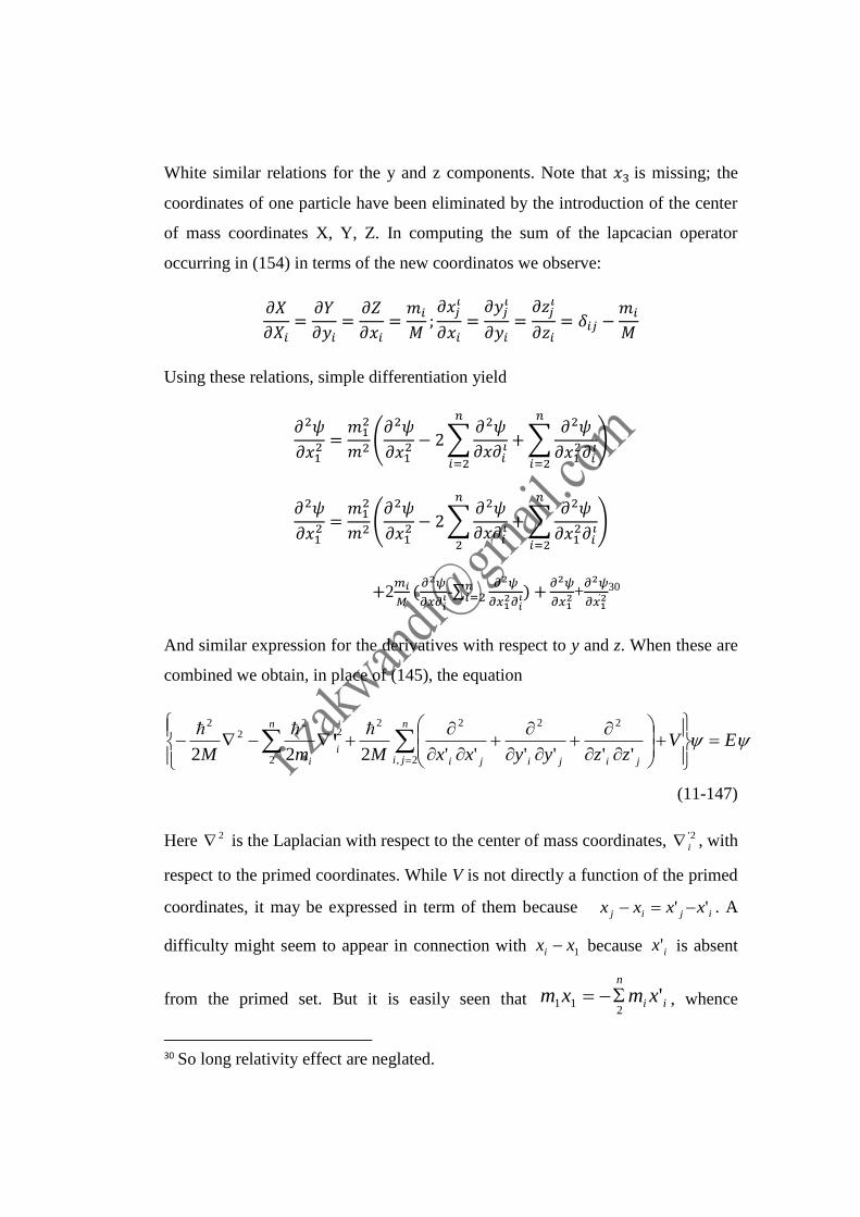
White similar relations for the y and z components. Note that 𝑥3 is missing; the

coordinates of one particle have been eliminated by the introduction of the center

of mass coordinates X, Y, Z. In computing the sum of the lapcacian operator

occurring in (154) in terms of the new coordinatos we observe:

𝜕𝑋

𝜕𝑋𝑖=𝜕𝑌

𝜕𝑦𝑖=𝜕𝑍

𝜕𝑥𝑖=𝑚𝑖

𝑀;𝜕𝑥𝑗

𝜄

𝜕𝑥𝑖=𝜕𝑦𝑗

𝜄

𝜕𝑦𝑖=𝜕𝑧𝑗

𝜄

𝜕𝑧𝑖= 𝛿𝑖𝑗 −

𝑚𝑖

𝑀

Using these relations, simple differentiation yield

𝜕2𝜓

𝜕𝑥12 =

𝑚12

𝑚 2(𝜕2𝜓

𝜕𝑥12 − 2∑

𝜕2𝜓

𝜕𝑥𝜕𝑖𝚤 +∑

𝜕2𝜓

𝜕𝑥12𝜕𝑖

𝚤

𝑛

𝑖=2

𝑛

𝑖=2

)

𝜕2𝜓

𝜕𝑥12 =

𝑚12

𝑚 2(𝜕2𝜓

𝜕𝑥12 − 2∑

𝜕2𝜓

𝜕𝑥𝜕𝑖𝚤 +∑

𝜕2𝜓

𝜕𝑥12𝜕𝑖

𝚤

𝑛

𝑖=2

𝑛

2

)

+2𝑚𝑖

𝑀(𝜕2𝜓

𝜕𝑥𝜕𝑖𝚤-∑

𝜕2𝜓

𝜕𝑥12𝜕𝑖

𝚤) +𝑛𝑖=2

𝜕2𝜓

𝜕𝑥12+

𝜕2𝜓

𝜕𝑥12

30

And similar expression for the derivatives with respect to y and z. When these are

combined we obtain, in place of (145), the equation

EVzzyyxxMmM

n

ji jijiji

n

ii

2,

2222

2

22

22

''''''222'

(11-147)

Here 2 is the Laplacian with respect to the center of mass coordinates, 2'

i , with

respect to the primed coordinates. While V is not directly a function of the primed

coordinates, it may be expressed in term of them because ijij xxxx '' . A

difficulty might seem to appear in connection with 1xxi because ix' is absent

from the primed set. But it is easily seen that ii

n

xmxm '2

11 , whence

30 So long relativity effect are neglated.

jj

n

ji

ii xmm

xxx ''1 . Therefore V, when expressed in term of new coordinates,

will not contain X, Y, or Z.

As result, eq. (147) is separable; therefore may be written as

).''(),,( 2 nzxZYX

Correspondingly, 'EEE c , where Ec is energy associated with ),,( ZYX ,

determined by

cEM

22

2

This is Schrὄdinger equation of a free particle of mass M, it produces, as

we know, no quantization. The remainder of (147) describes the internal motion

of the particles :

'22 2,

''2

2

'2

EVMm

n

ji

ji

n

i

i

(11-148)

It differs from the normal from Schrὄdinger’s equation by presence of the terms in

''

ji and by the fact that V has a different functional form in the primed

coordinates than in the unprimed ones.

The coordinates (146) measure the position of the i-th particles relative to

the center mass. It also possible to use a less symmetrical but physically more useful

set coordinates, which is closely related to (146). If we put

,,,,

,1

113

'

312

'

2'

11

xxxxxxxxx

mMxmM

X

nn

n

i

n

ii

(11-149)

Thus measuring all coordinates relative to that one which has been eliminated ( 1x

), we obtain in the same manner the equation

EVMmM

n

ji

ji

n

ii

2,

''2

2

22

22

222'

(11-150)

This form is particularly useful when it is desired to calculate the energy of a many-

electron atom, for particle 1 may then be taken to be the nucleus and summations

in (150) are extended electrons. The equations remaining after separation of the

motion of the center of mass is now

'11

2 ,

''

12

22

' EVmm

n

ji

ji

n

i

Where m is the mass of an electron, 1m , that of nucleus. If may be written in terms

of the reduced mass.

1

1

mm

mm

As follows :

'22

''

1

22'

2

EVm ji

ji

i

i

(11-151)

The terms in the double summation play an important role in the isotope effect of

heavy atoms.31

They are present whenever the number of electrons is greater than one. For the case

of hydrogen, eq.(151) has the same form as Schrὄdinger’s equation for a stationary

nucleus, except for the replacement of the electron mass by . Hence the true

energies of the hydrogen atom are not exactly given by eq.(64), but by that equation

with written from m. Note that the function V is different in (148) and (151), and

that the trms of the double summation have opposite signs. Nevertheless the

31 See Huges, A. L., and Eckart, C.,Phys. Rev. 36,694(1930)

equivalence of these two equations for the two-body problem may be seen as

follows. Write for the potential energy in (151)

),',','( zyxVV

Where

12' xxx , etc.

The V-function of (148) must then be expressed in terms ZzYyXx 222 ,, .

Now .2

1

2112 Xx

m

mmxx

Therefore we must use in (148)

,',','1

21

1

21

1

21

z

m

mmy

m

mmx

m

mmVV

And the equation reads

',','',','',','11

2

'2'

212

2

zyxEzyxzyxVmmm

Where

.1

21

m

mm If here we put ''',''',''' xzzyyxx it becomes :

','','',''''11

2

2

212

22

EzyxVmmm

Which is identical with eq. (151)

11.32. Independent System

Physical system are independent, or isolated from another, if Hamiltonian

operator of one contains no terms referring to another system. There is then no

interaction between them. Consider n independent systems, and let the coordinates

of the r-th system (including the spin coordinate) be symbolized by the single letter

qr. If its Hamiltonian operator is Hr its Schrὄdinger’s equation will be :

)()( )()()(

r

r

i

r

ir

r

ir qEqH (11-152)

)(r

iE being the i-th eigenvalue of the r-th system.

The state function describing the entire assemblage of n systems will satisfy

the equation

nnn qqqEqqqHHH 212121 ,, (11-153)

To find its solutions we put n

n

n qqqqqq )(

2

)2(

1

)1(

21,

tentatively. Substitution in (153) and use of the fact that 1H acts only on 1q , etc.,

leads at once to the equation

EHHH

n

n

n )(

)(

)2(

)2(

2

)1(

)1(

1

Which show that each term )(

)(

r

r

rH

is separately a constant, say )(rE and that

the sum of all these constant is E. But if )(

)(

)(r

r

r

r EH

then

)(r must be one of

the energies )(r

iE , Therefore

)()2()1(

)(

2

)2(

1

)1(

21 ,

n

sji

n

n

n

EEEE

qqqqqq

(11-154)

This result in indeed what intuition would lead us to expect. For clearly the total

energy of a number of isolated system is the sum of the individual energies.

Furthermore, if 1w is the probability that system 1 be found at 21, wq that system 2

be found at 2q , then the probability that both of these statements be true

simultaneously is product 21ww . Hence the individual functions, whose squares

are these probabilities, must like-wise combine as factors.

This latter circumstance is dictated also by the time dependence of the

Schrὄdinger’s states eq. (113). For only the product of the individual function

.,,,)2()1( )/()2()/()1( etcee tEitEi will have the

r

r tEi

e

)()/(

required in

Eti

n eqqq )/(

,,2,1 )( .

11.33. The Exclusion Principle.

When two independent systems occupy the energy states )1(

iE and )2(

jE

respectively, the combine system has an energy

)2()1(

ji EEE

And a state function

)2()( )2(

1

)1( qq ji (11-155)

We shall suppose for the moment that the individual states )1(

i and )2(

j are

non-degenerate. Then, unless there happen to be two energies )1(

lE and )2(

kE whose

sum is precisely the same as)2()1(

ji EE , the combined state (155) will also be non-

degenerated. This will generally be the case when the two systems are different in

a physical sense.

But if they are similar, e.g., both electrons or both hydrogen atoms, another

situation arises. We may then drop all superscripts in the description of the states,

and write (155)

)()(, 21

)2()1( qqEEE jiji (11-156)

This state is degenerate, although i and j are not; for if we interchange

the result a different function but not a different energy. This degeneracy,

which is peculiar to the description of any aggregated of similar systems, is known

as exchange degeneracy. Classically it implies that the energy of the total system is

unaltered when two individual constituents exchange place and spins.

In the more general case where iE has ig and jE has jg linearly

independent function associated with it, the number of ' s corresponding to E will

be, not ji gg but ji gg2 .

Returning to the case of non-degeneracy of i and j we not that the two

functions

)()(),()( 2121 qqqq ijIIjiI

Which are linearly independent, are equally good representatives of the state

in which ji EEE . Moreover, any linear combination of the two satisfies the

Schrὄdinger’s equation for this value of E, and has just claim to be considered. Of

course, only two such combinations can be linearly independent. Let us then

consider the function

III ba

Where we shall assume 122 ba to assure normalization. On “exchanging” the

two systems, III and III , hence the function above transforms itself

into

III ab

The numerical value of which for any given configuration 21,qq will in general be

different from III ba . Physically, this implies that the configuration which

result when the two systems exchange places has an altogether different probability

than the original, a consequence that is clearly objectionable.

However, among all linear combinations there are two which avoid this

dilemma. They are the symmetri32

combination

IIIs qq 2

1, 21

And the “ antisymmetric ” one

IIIA qq 2

1, 21

They are independent and indeed orthogonal; the first remains unaltered on

exchange of systems, the second change its sign. Both, therefore, yield probabilities

2 which are insensitive to exchange.

Consider now, not two, but n independent similar system, in states

,,, sji . The assemblage has energy sji EEEE , and is describe by the

state function

nsjin qqqqqq 2121, (11-157)

Where every permutation of the q’s among the ' s on the right will produce a new

function belonging to the same E, provided the subscripts, sji , are all different

(which we shall assume for the moment). Hence, if P np qqq 21, the function

which result from (157) when this permutation is made, then

p

ppn aqqq 21, (11-158)

32 A function is said to be symmetric with respect to a given operation if the operation leaves it

unchanged; it is said (in quantum mechanics) to be antisymmetric if the operation changes its sign

without altering it in any other way.

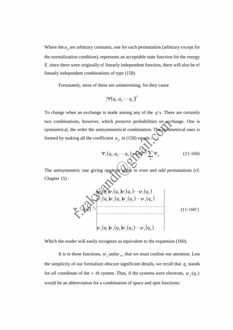
Where the pa are arbitrary constants, one for each permutation (arbitrary except for

the normalization condition), represents an acceptable state function for the energy

E. since there were originally n! linearly independent function, there will also be n!

linearly independent combinations of type (158)

Fortunately, most of these are uninteresting, for they cause

2

21, nqqq

To change when an exchange is made among any of the 'q s. There are certainly

two combinations, however, which preserve probabilities on exchange. One is

symmetrical, the order the antisymmetrical combination. The symmetrical ones is

formed by making all the coefficient pa in (158) equals :

p

pns nqqq 21

21 !, (11-160)

The antisymmetric one giving opposite signs to even and odd permutations (cf.

Chapter 15) :

nssss

njjjj

niiii

A

qqqq

qqqq

qqqq

n

321

321

321

21

! (11-160’)

Which the reader will easily recognize as equivalent to the expansion (160).

It is to these functions, s and A , that we must confine our attention. Lest

the simplicity of our formalism obscure significant details, we recall that rq stands

for all coordinate of the r -th system. Thus, if the systems were electrons, )( rj q

would be an abbreviation for a combination of space and spin functions:

rrrrjrrrrj szyxszyx ,,,,

In the notation of sec. 29, and an interchange of rq and pq means that rx is to be

exchanged against rp zx , against rp zy , against pz and rs against ps .

There is no a priori way of deciding which of the two function, (159) or

(160), is preferable. But here the exclusion principle, early recognized by Pauli,

creates simplicity in a most effective way. It states that if the individual systems

belong to a certain class (see below), only antisymmetric functions may be used in

describing the assemblage. This principle is of the nature of postulate; it has not yet

been deduced from more fundamental axioms, although one might hope, from a

mathematical point of view, that this will prove possible.33

Why nature insist upon antisymmetric states for some and symmetric states for

other among its creatures is at present a puzzle.

The elementary systems which Pauli’s principle is known to apply are;

electrons, positrons, protons, neutrons, neutrinos, and mu-mesons; photons, on the

other hand, and several kind of meson, are described by symmetrical state functions.

Perhaps the most important consequence of the exclusion principle is this.

Suppose our assemblage consist of electrons, two of which are described by the

same function i (i.e., the functions are identical with respect to positional and spin

factors). The determinant (160’) will then have two equal rows, and hence will

vanish. We may therefore say: two systems obeying the Pauli principle cannot be

in the same state. This fact governs the structure of atoms and molecules; each

electrons added to the shell of an atom must have its own set of quantum numbers.

33 A very searching and interesting examination of the principle in the light of other fundamental

issue has been given by Pauli, Phy. Rev. 58, 716 (1940)

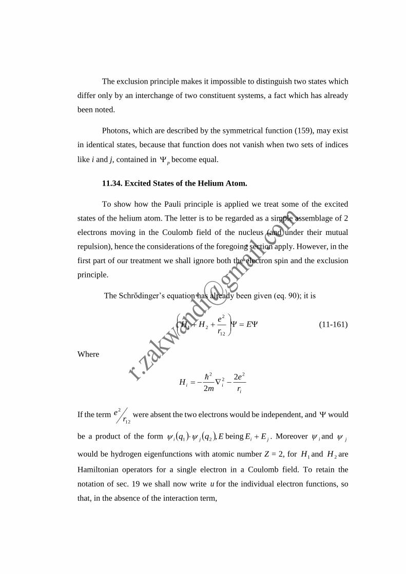
The exclusion principle makes it impossible to distinguish two states which

differ only by an interchange of two constituent systems, a fact which has already

been noted.

Photons, which are described by the symmetrical function (159), may exist

in identical states, because that function does not vanish when two sets of indices

like i and j, contained in p become equal.

11.34. Excited States of the Helium Atom.

To show how the Pauli principle is applied we treat some of the excited

states of the helium atom. The letter is to be regarded as a simple assemblage of 2

electrons moving in the Coulomb field of the nucleus (and under their mutual

repulsion), hence the considerations of the foregoing section apply. However, in the

first part of our treatment we shall ignore both the electron spin and the exclusion

principle.

The Schrὄdinger’s equation has already been given (eq. 90); it is

E

r

eHH

12

2

21 (11-161)

Where

i

iir

e

mH

22

2 2

2

If the term 12

2

re were absent the two electrons would be independent, and would

be a product of the form Eqq ji ,21 being ji EE . Moreover i and j

would be hydrogen eigenfunctions with atomic number Z = 2, for 1H and 2H are

Hamiltonian operators for a single electron in a Coulomb field. To retain the

notation of sec. 19 we shall now write u for the individual electron functions, so

that, in the absence of the interaction term,

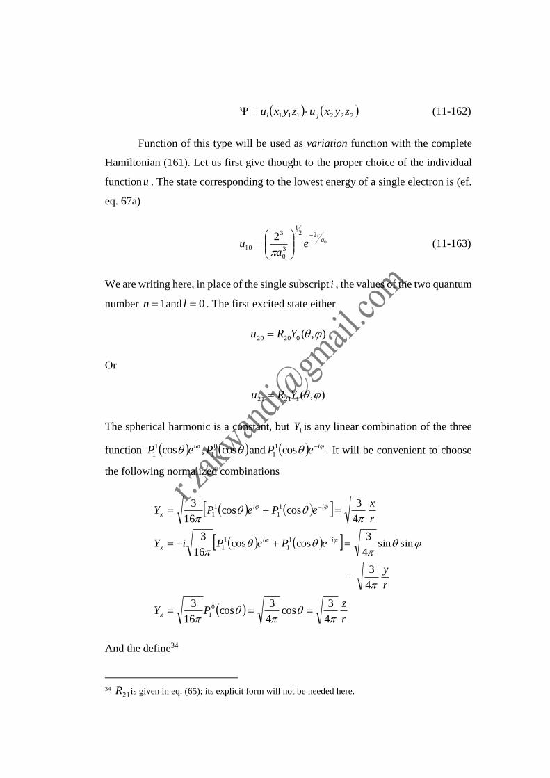
222111 zyxuzyxu ji (11-162)

Function of this type will be used as variation function with the complete

Hamiltonian (161). Let us first give thought to the proper choice of the individual

functionu . The state corresponding to the lowest energy of a single electron is (ef.

eq. 67a)

0

221

3

0

3

10

2 ar

ea

u

(11-163)

We are writing here, in place of the single subscript i , the values of the two quantum

number 1n and 0l . The first excited state either

),(02020 YRu

Or

),(12121 YRu

The spherical harmonic is a constant, but 1Y is any linear combination of the three

function cos,cos 0

1

1

1 PeP iand ieP cos1

1 . It will be convenient to choose

the following normalized combinations

r

zPY

r

y

ePePiY

r

xePePY

x

ii

x

ii

x

4

3cos

4

3cos

16

3

4

3

sinsin4

3coscos

16

3

4

3coscos

16

3

0

1

1

1

1

1

1

1

1

1

And the define34

34 21R is given in eq. (65); its explicit form will not be needed here.

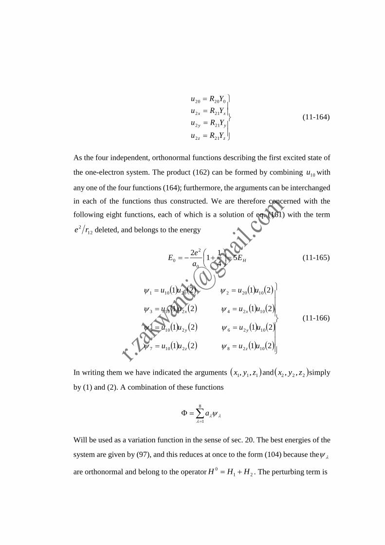
zz

yy

xx

YRu

YRu

YRu

YRu

212

212

212

02020

(11-164)

As the four independent, orthonormal functions describing the first excited state of

the one-electron system. The product (162) can be formed by combining 10u with

any one of the four functions (164); furthermore, the arguments can be interchanged

in each of the functions thus constructed. We are therefore concerned with the

following eight functions, each of which is a solution of eq. (161) with the term

12

2 re deleted, and belongs to the energy

HEa

eE 5

4

11

2

0

2

0

(11-165)

2121

2121

2121

2121

10282107

10262105

10242103

1020220101

uuuu

uuuu

uuuu

uuuu

zz

yy

xx

(11-166)

In writing them we have indicated the arguments 111 ,, zyx and 222 ,, zyx simply

by (1) and (2). A combination of these functions

8

1

a

Will be used as a variation function in the sense of sec. 20. The best energies of the

system are given by (97), and this reduces at once to the form (104) because the

are orthonormal and belong to the operator 21

0 HHH . The perturbing term is

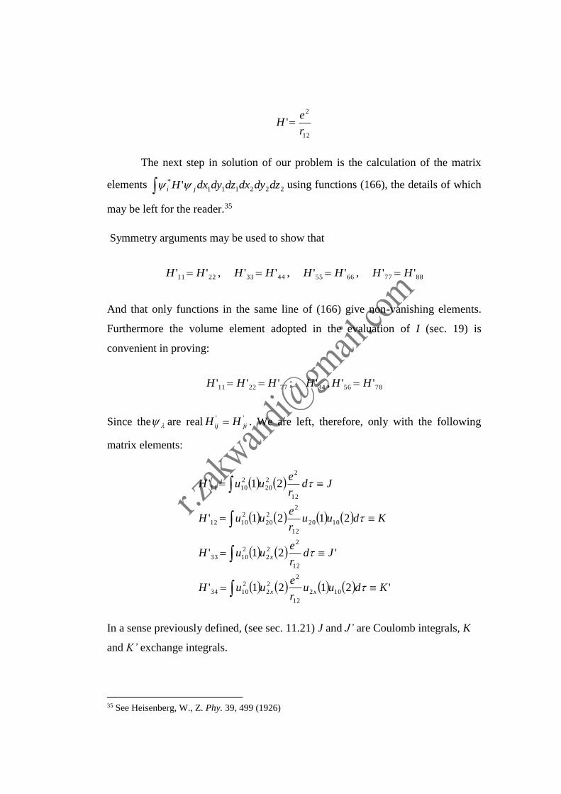
12

2

'r

eH

The next step in solution of our problem is the calculation of the matrix

elements 222111

* ' dzdydxdzdydxH ji using functions (166), the details of which

may be left for the reader.35

Symmetry arguments may be used to show that

8877665544332211 '','','','' HHHHHHHH

And that only functions in the same line of (166) give non-vanishing elements.

Furthermore the volume element adopted in the evaluation of I (sec. 19) is

convenient in proving:

785634772211 '',';''' HHHHHH

Since the are real''

jiij HH . We are left, therefore, only with the following

matrix elements:

'2121'

'21'

2121'

21'

102

12

22

2

2

1034

12

22

2

2

1033

1020

12

22

20

2

1012

12

22

20

2

1011

Kduur

euuH

Jdr

euuH

Kduur

euuH

Jdr

euuH

xx

x

In a sense previously defined, (see sec. 11.21) J and J’ are Coulomb integrals, K

and K’ exchange integrals.

35 See Heisenberg, W., Z. Phy. 39, 499 (1926)

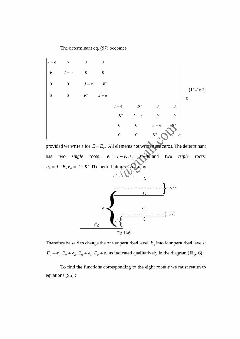
The determinant eq. (97) becomes

0

'00

'00

00'

00'

'00

'00

00

00

eJK

KeJ

eJK

KeJ

eJK

KeJ

eJK

KeJ

(11-167)

provided we write e for .0EE All elements not written are zeros. The determinant

has two single roots: ', 21 KJeKJe and two triple roots:

'',' 43 KJeKJe The perturbation 12

2 re may

Therefore be said to change the one unperturbed level 0E into four perturbed levels:

,40302010 ,,, eEeEeEeE as indicated qualitatively in the diagram (Fig. 6).

To find the functions corresponding to the eight roots e we must return to

equations (96) :

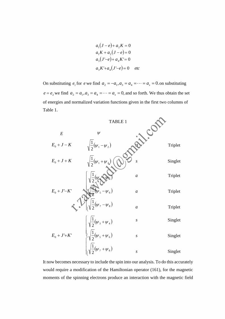
etceJaKa

KaeJa

eJaKa

KaeJa

0''

0''

0

0

43

43

21

21

On substituting 1e for e we find .0, 4312 saaaaa on substituting

2ee we find ,0, 4312 saaaaa and so forth. We thus obtain the set

of energies and normalized variation functions given in the first two columns of

Table 1.

TABLE 1

E

KJE 0 212

1 a Triplet

KJE 0 212

1 s Singlet

''0 KJE

87

65

43

2

1

2

1

2

1

a

a

a

Triplet

Triplet

Triplet

''0 KJE

87

65

43

2

1

2

1

2

1

s

s

s

Singlet

Singlet

Singlet

It now becomes necessary to include the spin into our analysis. To do this accurately

would require a modification of the Hamiltonian operator (161), for the magnetic

moments of the spinning electrons produce an interaction with the magnetic field

do their orbital motions and this interaction has not been included in (161). We shall

omit this spin-orbit interaction and refer the reader to the literature for the more

accurate treatment.36

In other words, we shall suppose that the Hamiltonian does not act on the spin

coordinates. The state function is then separable and appears as the product of an

orbital (any of the functions in the table) and a spin function, and the letter may be

taken as an eigenfunction of z for each electron. Let us consider these spin function

more closely. For the two electrons, we have four functions:

11111111 ,,, ssandssssss

These, however, do not have convenient exchange properties, for when 1s and 1s are

interchanged, the first and last remain unaltered, the second transforms into the third

two other, equivalent functions, which are symmetrical with respect to an exchange

of spin coordinates. They are, when normalized, 21212

1ssss and

21212

1ssss . We have in this way obtained four spin functions

)16811(2

1

;,2

1,

2121

3 212 21211 21

ssssA

ssssssss

The first three of which are symmetrical, only the last being antisymmetrical.

Furthermore, this set of function is orthogonal (and complete).

To include the spin we need only multiply each one of the functions in Table

1 by one of the spin functions 1to A , a procedure which yields 32 different

functions of position and spin coordinates. But here the exclusion principle effects

36 Condon, E. U., and Shortley, G. H., “The Theory of Atomic Spectra,” Macmillan Co. New

York, 1953

a great simplification. It says that only functions which are antisymmetrical when

all coordinates, i.e., position and spin coordinates, of the two electrons are

interchanged, are to be permitted. Hence a function of Table 1 which is symmetrical

can only be combined with A , and a function which is antisymmetrical only with

1 2, and .

3

Now the functions marked a in the table are antisymmetric; they can be

multiplied by any one of the three functions. Each of them corresponds,

therefore, to three states. For this reason the energy states ''0 KJE and

KJE 0 are said to be triplet states. If spin-orbit interaction had been included

in our calculation each of these levels would have appeared as three closely adjacent

levels, while the other energies, marked singlet, would have remained single.

It is true that the functions in Table 1 are only approximate solutions of eq.

(161). Nevertheless what we have said about their symmetry with respect to

exchange of electrons may be shown to hold rigorously. The structure of the helium

energy spectrum, and in particular the singlet-triplet character of the states, are

therefore correctly given by the simple theory of this section; the numerical values

of the energy levels will be in error.

The normal state of helium atom, whose energy was computed

approximately in sec. 19 of this chapter, is given in the present notation by

21 1010 uu , if we neglect the spin. It is clearly symmetrical and can only be

multiplied by A when the spins are introduced. Hence it is a singlet state. When the

helium atom is in a singlet state, its probability is very small, as may be shown by

an extension of the methods used in sec. 11.28. Hence triplet and singlet levels so

not “ combine, “ and helium may be said to have two distinct spectra, the triplet

spectrum, to which spetrocopist apply the term “ orthohelium “ spectrum, and the

singlet spectrum called “ parhelium “ spectrum.

Problem a. Instead of using the 8 functions (166) as linear variation

function s, star with the 32 functions obtained from (166) by multiplying each of

them by 1 2 3.,, A Show that, if these 32 functions are suitably arranged, the

determinant equation is a four-fold repetition of the one obtained above, and that it

yields the same result in regard to both energies and functions.

Problem b. the following spin operators for two electrons may be defined:

212121

2

2

2

2

2

2

2

1

2

1

2

1

2

21

2

21

2 zzyxyxxzyxzyx

zzz

where 1x is the operators z acting on spin coordinate ,1s etc. Show that

1 2 3.,, and A are all eigenstates with respect to both of these operators, in

particular that

0,8,8,8

0,2,0,2

2

33

2

22

2

11

2

33211

A

Azzzz

Are these result consistent with the classical interpretation according to which

1is the state in which both spin are parallel and along Z,

2is the state in which both spin are parallel and perpendicular to Z,

3is the state in which both spin are parallel and along to Z,

A is the state in which both spin are opposed and yield no resultant angular

momentum?

11.35. The Hydrogen Molecule,

One of the stumbling blocks of pre-quantum chemistry was the phenomenon of

homo-polar binding; it is impossible to explain on the basis of classical dynamics

the union of two hydrogen atoms to form a molecule. They only attraction which

two neutral structures like H-atoms could possibly exhibit was due to quadru-pole

forces, and these were known to be too weak to account for molecular binding. It

was shown by Heitler and London that the homo polar bond it caused by a typical

quantum-mechanical effect: the “exchange“ of the two electrons. Its meaning will

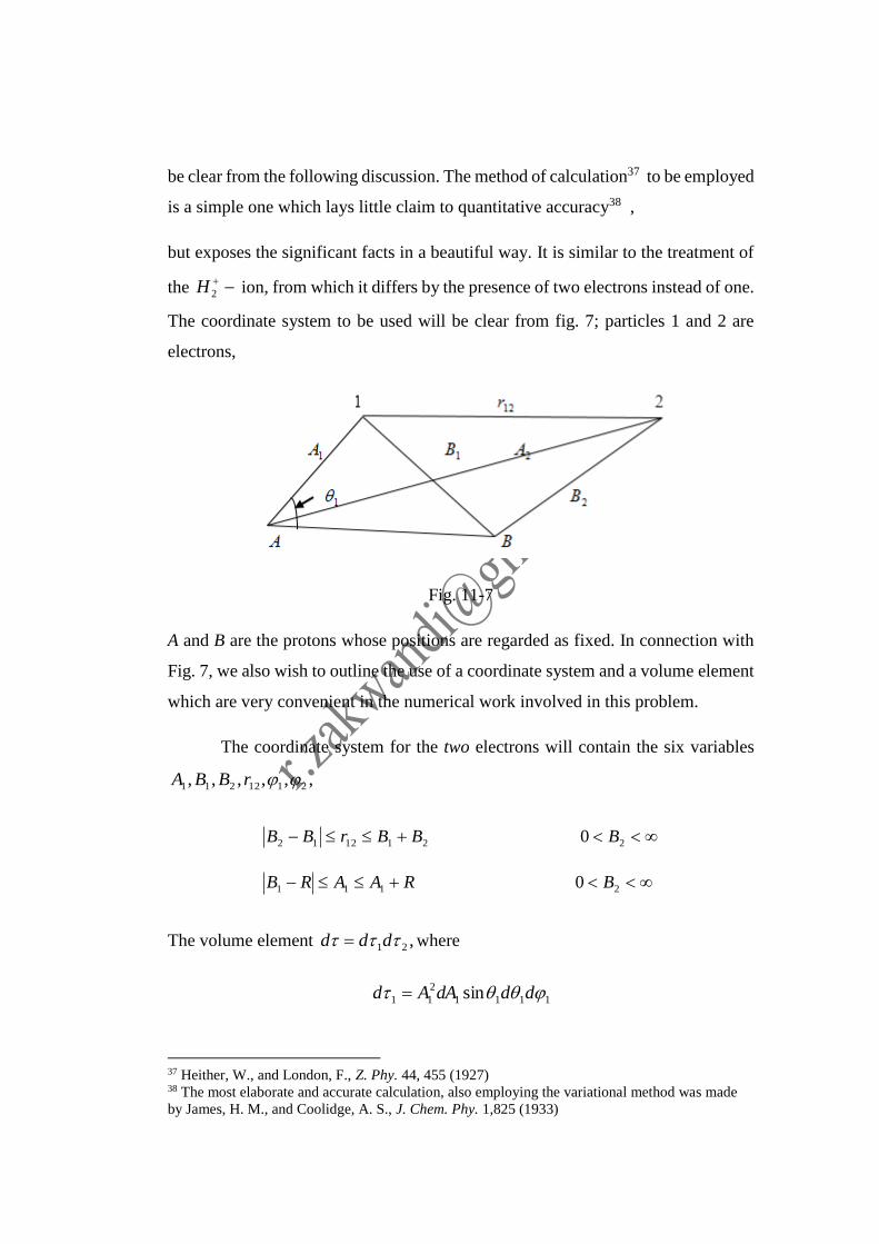
be clear from the following discussion. The method of calculation37 to be employed

is a simple one which lays little claim to quantitative accuracy38 ,

but exposes the significant facts in a beautiful way. It is similar to the treatment of

the

2H ion, from which it differs by the presence of two electrons instead of one.

The coordinate system to be used will be clear from fig. 7; particles 1 and 2 are

electrons,

Fig. 11-7

A and B are the protons whose positions are regarded as fixed. In connection with

Fig. 7, we also wish to outline the use of a coordinate system and a volume element

which are very convenient in the numerical work involved in this problem.

The coordinate system for the two electrons will contain the six variables

,,,,,, 2112211 rBBA

2111

2211212

0

0

BRAARB

BBBrBB

The volume element ,21 ddd where

1111

2

11 sin dddAAd

37 Heither, W., and London, F., Z. Phy. 44, 455 (1927) 38 The most elaborate and accurate calculation, also employing the variational method was made

by James, H. M., and Coolidge, A. S., J. Chem. Phy. 1,825 (1933)

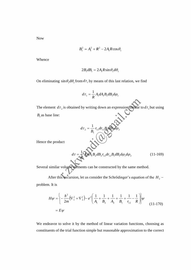
Now

11

22

1

2

1 cos2 RARAB

Whence

11111 sin22 dRAdBB

On eliminating 11sin d from by means of this last relation, we find

111111

1 ddBBdAA

Rd

The element 2d is obtained by writing down an expression similar to 1d but using

1B as base line:

2221212

1

2

1 ddBBdrr

Bd

Hence the product

211112122211

1 dddBBdrrdBBdAA

Rd (11-169)

Several similar volume elements can be constructed by the same method.

After this excursion, let us consider the Schrὄdinger’s equation of the 2H

problem. It is

E

RrBABAe

mH

111111

2 121221

22

2

2

1

2

(11-170)

We endeavor to solve it by the method of linear variation functions, choosing as

constituents of the trial function simple but reasonable approximation to the correct

1d

. If H did not contain the last four items in the parenthesis multiplying 2e it would

simply be the sum of two hydrogen-atom Hamiltonian, and

21 BA uu

Where

0

2

0

1

21

3

02

13

0 2,1

B

B

A

A eaueau

Are hydrogen functions centered about A and B respectively. On the other hand,

in the terms RrBA 1111 1221 were missing from the parenthesis, H would

also be the sum of two hydrogen-atom Hamiltonians, but 21 AB uu . Both the

these ’s are equally good approximations, and both must be included in the trial

function. Note that they differ with respect to an exchange of the electrons (or,

amounts in this problem to the same thing, the protons). Hence we adopt

2121 21 ABBA uucuuc (11-170)

As variation function in minimizing dH . As explained in sec. 20, the process

leads to the secular equations

0cc

0cc

2222221211

1212211111

EE

EE

(11-171)

And E given by

0

22222121

12121111

EE

EE

(11-172)

Here

21

2

12112

2221

22

11

112121

121

duudduuuu

dduu

BAABBA

BA

The letter integral is familiar from sec. 21, it is the quantity there called AB .

Hence

0

22

2

2112 ,3

1

R

e p

Next, we turn to

2111 1121 dduHuuu AABA

The 2 terms in H need not calculated; their effect upon 1Au and 2Bu is at

once obtainable from the differential equations which these function satisfy:

222

,112

2

22

2

2

1

22

1

2

BHB

AHA

uB

eEu

m

uA

eEu

m

In this way we find

R

eJJEH

2

11 '22

Where

1

1

22

21

1

1

222 121 d

B

ueddBuueJ A

BA (11-173)

And

1

1

22

21

12

222 121

' dB

uedd

r

uueJ ABA (11-174)

J is given in sec. 21, eq. (100), and J’ has the value

64

3

8

1111' 22

2 e

R

eJ

Problems. Prove this result, using the system of coordinates and the volume

element (169).

Furthermore,

1122

As the reader will easily verify. In a similar way,

12

2

21

12122112 '22 R

eKEEH

Where

1

1

1

2 11 dBuueK BA (11-175)

And

21

12

1

12 2211 dd

r

uuBuueK BABA

(11-176)

The value of K is given in eq. (100), and

4'2'2ln6

3

13

4

23

8

25

5' 322

0

2

EiEi

ee

K

Where 5772,0 (Euler-Mascheroni constant),

22

2

123

1',

e

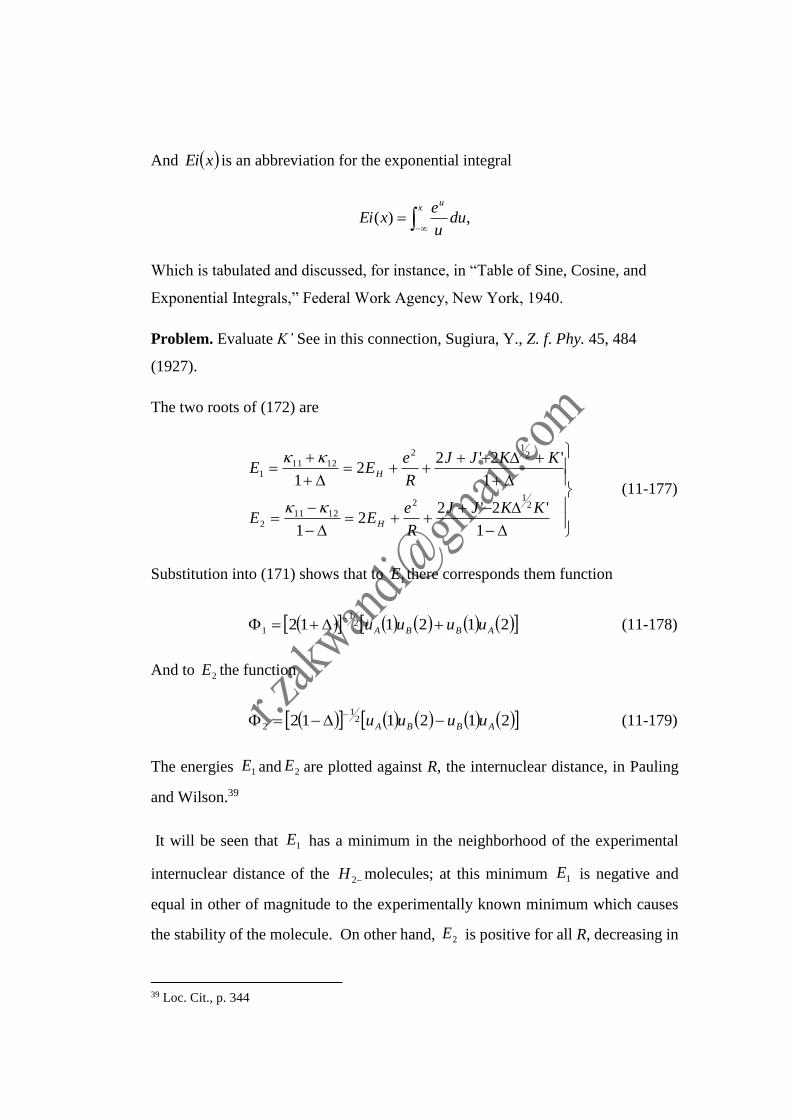
And xEi is an abbreviation for the exponential integral

xu

duu

exEi ,)(

Which is tabulated and discussed, for instance, in “Table of Sine, Cosine, and

Exponential Integrals,” Federal Work Agency, New York, 1940.

Problem. Evaluate K’ See in this connection, Sugiura, Y., Z. f. Phy. 45, 484

(1927).

The two roots of (172) are

1

'2'22

1

1

'2'22

1

21

2

12112

21

2

12111

KKJJ

R

eEE

KKJJ

R

eEE

H

H

(11-177)

Substitution into (171) shows that to 1E there corresponds them function

212112 21

1 ABBA uuuu

(11-178)

And to 2E the function

212112 21

2 ABBA uuuu

(11-179)

The energies and are plotted against R, the internuclear distance, in Pauling

and Wilson.39

It will be seen that has a minimum in the neighborhood of the experimental

internuclear distance of the 2H molecules; at this minimum is negative and

equal in other of magnitude to the experimentally known minimum which causes

the stability of the molecule. On other hand, is positive for all R, decreasing in

39 Loc. Cit., p. 344

1E 2E

1E

1E

2E

monotone fashion with increasing R.it, therefore corresponds to repulsion between

the atoms. Comparison of and shows the difference in their behavior as

function or R to be predominantly due to the presence of the K and K’ integrals.

These would have been missing if electron had not been taken account of by

introducing the two functions constituting the of eq. (170). In that case also, there

would have been only one energy and not two. Now while (170) may be crude

approximation, the fact that two equivalent functions, differing only with respect to

electron exchange, will compose the correct solution of (170) is beyond doubt,

hence the qualitative aspect here obtained cannot be questioned. The integrals K

and K’ are called exchange integrals.

Let us now included the spin and apply the Pauli principle. The spin function

are those already encountered in the helium problem, eq. (168). If the resultant

function is to be antisymmetrical, 1 , which is symmetrical in the position

coordinates of electrons 1 and 2must be multiplied by an antisymmetrical function

of the spins, of which there is only one, namely A . However, 2 may be multiplied

by one of the three functions 1 2 3or . It represent a triplet state while is

singlet.

To the energy , therefore, there correspond three times as many quantum

mechanical states as to 1E . From this fact may be drawn the conclusion that when

H-atoms approach they will, ceteris paribus, be three times as likely to repel as to

attract each other.

REFERENCES

To begin with source material, there are : Schrӧdinger’s charming volume

“Wave mechanics” (Blackie and Son, London, 1932) which is a collection of this

epoch-making papers of 1926 and 1927; Heisenberg’s more popular “The physical

Principles of the quantum theory” (Chicago University Press, Chicago, 1930); De

Broglie and Brillouin’s and Jordan’s “Elementare Quantenmechanik” (J. Springer,

Berlin, 1930) The foundations of the subject, both mathematical and philosophical,

1E 2E

1

2E

are treated most thoroughly but also most abstractly by Dirac in his “Principle of

Quantum Mechanics” (Clarendon Press, Oxford, Third Edition, 1947) and by J. v.

Neumann in “Mathematische Grundlagen der Quantenmechanic” (J. Springer,

Berlin, 1932)

General treatises are :

Condon, E. U., and Morse, P. M., “Quantum Mechanics,” McGrew-Hill Book Co.,

Inc., New York, 1929.

Ruark, A. E., and Urey, H. C., “Atoms, Molecules, and Quanta,” McGrew-Hill Co.,

Inc., New York, 1930

De Broglie, L., “Theorie de la Quantification,” Hermann et Cie, Paris, 1932.

Frenkel, J., ”Wave Mechanics,” Vols. I and II, Clarendon Press, Oxford, 1932,

1934.

“Handbuch der Physisk,” Vol. XXIV, Parts I and II (numerous author), Julius

Springer, Berlin, 1933.

Pauling. L., and Wilson, E. B., “Introduction of Quantum Mechanics,” McGrew-

Hill Co., Inc., New York, 1935

Jordan. P., “Anschauliche Quantenmechanik,” J. Springer, Berlin, 1936.

Kemble, E. C., “The fundamental Principles of Quantum Mechanics,” McGrew-

Hill Co., Inc., New York, 1937.

Dushman, S., “Elements of Quantum Mechanics,” John Wiley and Sons, Inc., New

York, 1938.

Sommerfeld, A., “Atombau und Spektrallinien,” Vol. II, Vieweg und sons,

Braunschweig, 1939.

Mott, N. F., and Sneddon, I. N., “Wave mechanics and its Applications” Oxford

Press, 1948.

Schiff, L. I., “Quantum Mechanics,” McGrew-Hill Co., Inc., New York, 1949

Bohm, D., “Quantum Theory,” Prentice-Hall, Inc,. New York, 1951.

Slater, J. C., “Quantum Theory of Matter,” McGrew-Hill Co., Inc., New York, 1951

Houston, W. V., “Principles of Quantum Mechanics,” McGrew-Hill Co., Inc., New

York, 1951

Lande, A., “Quantum Mechanics” Pitman Publishing Corp., New York, 1951

A list books in which quantum mechanics is applied to special problems

follows.

Van Vleck, J. K., “The Theory of Electric and Magnetic Susceptibilities,”

Clarendon Press, Oxford, 1932.

Condon, E. U., and Shortley, G. H., “The Theory of Atomic Spectra,” The

Macmillan Co., New York, 1935.