Performance OR Capacity #CMGimPACt2016

Different Approaches for Different TasksCMG imPACt 2016

42nd International Conference by Computer Measurement Group

Alexander Gilgur, Steve Politis

Session 361

November 08, 2016 La Jolla, CA USA

Steve PolitisJosue KuriAlex NikolaidisGrace SmithYuri SmirnovTyler PricePaul Sorenson

For contributing knowledge, ideas, solutions, and support

What’s the difference between Performance

and Capacity?

• Two languages in the IT world

• Need tools, metrics, and stats compatible with both languages

• Need fluency in both languages

• Metrics:• Time (latency)• Rate• Count:

• Packets in flight• Packet loss

• A few words about % Utilization

• Models:• Correlations• Trends in Data• Time-Series Analysis

• Approach• Top-Down?• Bottom-Up?• Hybrid?

• Measures and Aggregations:• 𝜇 + 𝑍 ∗ 𝜎• Busy Hour/Peak Minute• Nonparametric Measures:

• P95• Outlier Boundaries

For Capacity Planning:• Uncertainty: “Redistribution of wealth”• Distribution Looks Gaussian• Washout of local anomalies

For Performance Analysis:• “Big Picture” • Immediate impact assessment• Drilldown is easier than aggregation:

• No need to worry about which aggregation function to choose

For Performance Analysis:• Immediate anomaly detection• Trend identification

• Practical Significance is unknown

For Capacity Planning:• ”Just the right” bandwidth• Actual distributions & trends

• Time Consuming• Aggregation can get complicated

• Aggregate AZ Pairs (“Flows”) for each service (product)• Aggregate services (products) for each AZ Pair

For Infra Performance Analysis:• Cannot tell where the “hot” issues are

For Capacity Planning:• Can tell how much each svc (product) needs

For Infra Performance Analysis:• Will ID “hot” flows (A-Z Pairs)

For Capacity Planning:• Will not find “hot” services(products)


• Packets in flight• Packet loss

• A few words about % Utilization

• Models:• Correlations• Trends in Data• Time-Series Analysis

• Approach• Top-Down?• Bottom-Up?• Hybrid?

• Measures and Aggregations:• 𝜇 + 𝑍 ∗ 𝜎• Busy Hour/Peak Minute• Nonparametric Measures:

• P95• Outlier Boundaries

[𝜇 − 𝑍 ∗ 𝜎, 𝜇 + 𝑍 ∗ 𝜎]

• The 𝑍 is arbitrary• Assumptions about the distribution:

• Mean and Variance defined• Gaussian (Symmetrical)• Stationary• No outliers

• Simple math:• Addition• Regression• TSA Forecasting

[𝜇 − 𝑍 ∗ 𝜎, 𝜇 + 𝑍 ∗ 𝜎] [𝜇 − 𝑍𝟏 ∗ 𝜎, 𝜇 + 𝑍𝟐 ∗ 𝜎]

𝑆𝑎𝑚𝑝𝑙𝑖𝑛𝑔:With enough random samples, their means will be Gaussian (Central Limit Theorem)

𝐷𝑎𝑡𝑎𝑇𝑟𝑎𝑛𝑠𝑓𝑜𝑟𝑚𝑎𝑡𝑖𝑜𝑛:• log• exp• Box-CoxFor Capacity Planning: For Monitoring:

Busy Hour / Peak Minute

Losing information:• Can’t identify the day’s outliers.• Need 3+ wks. of daily peaks to measure p95.

For Performance Monitoring

For Capacity Planning

• 𝑆𝑖𝑔𝑛𝑎𝑙 ∶ 𝑁𝑜𝑖𝑠𝑒 → 0.• Top-Down forecast is hard to interpret.• Misses underlying services.• Hides trends.

If used as an aggregated measure (Top-Down),• Accurate representation of Multiplexing.• Drilldown answers the “Who is hit the most?” question

• We size for busy-hour traffic.• Snapshot of service distribution:

• Great for Top-Down approach.

Nonparametric: p95

• Sensitive to Aggregation Level: • ∑𝑝95�

� (𝑥G) ≠ 𝑝95(∑𝑥𝑖�� ).• Have to have 20+ latest data points (𝑝95 ≡ K

LM)• How many of these are outliers?

For Performance Monitoring For Capacity Planning

• Summation may lead to oversizing• Ignores the bulk of the distribution• We will miss SLA 5% of the time• Forecasting p95: ergodicity assumption

• Distribution shape does not matter• OK to have outliers• Only 5% of data points will cause alerts • Easy to understand

• “Tradition!”• Math implemented in R, Python, Matlab, SAS

• even for regression

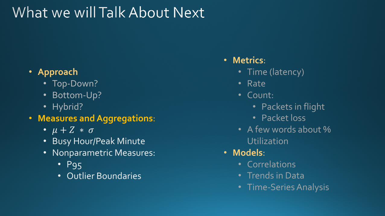
Should we Size Hardware for 𝒑𝟗𝟓 ?

5% of the time SLO (99.9%? 99.999%?) will be violated

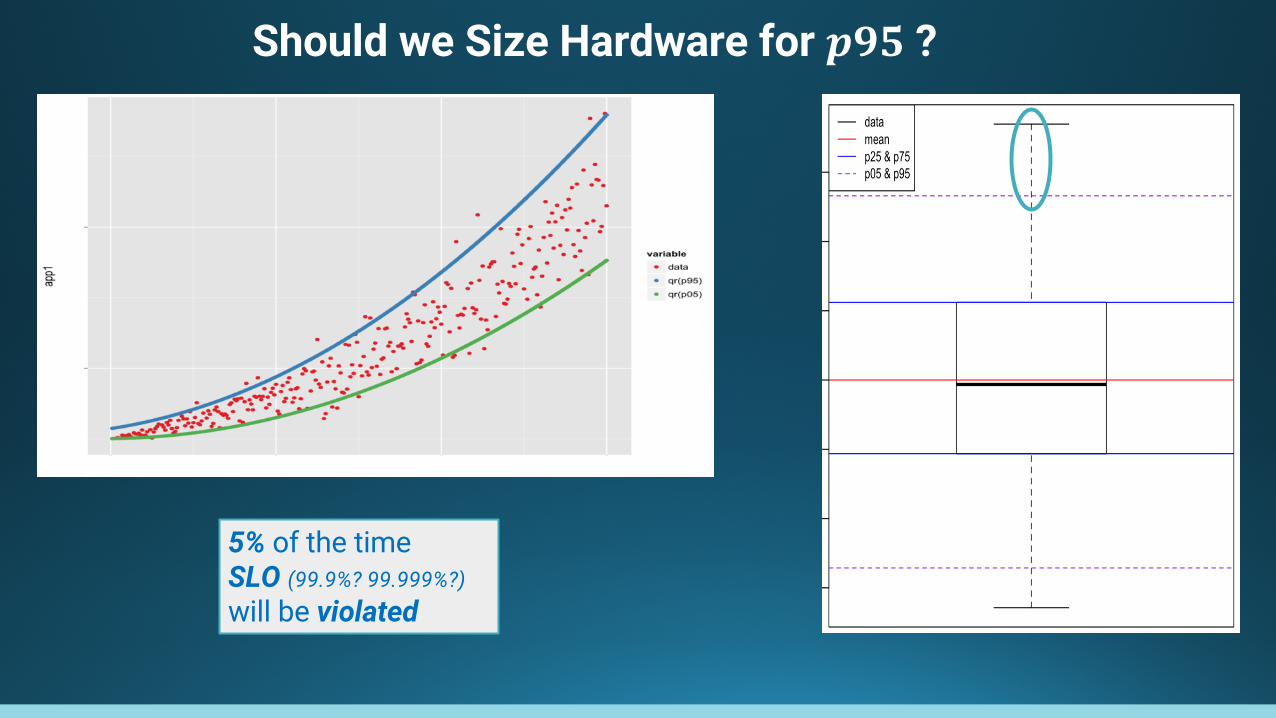
Shouldn’t we Size Resources for Non-Outliers Instead?

We size for SLA, as long as traffic stays within outlier boundaries

John Tukey’s IQR method:

𝐼𝑄𝑅 = 𝑝75 − 𝑝25𝐿𝑜𝑤𝑒𝑟𝐵𝑜𝑢𝑛𝑑 = 𝑝25 − 𝜷 ∗ 𝐼𝑄𝑅𝑈𝑝𝑝𝑒𝑟𝐵𝑜𝑢𝑛𝑑 = 𝑝75 + 𝜷 ∗ 𝐼𝑄𝑅

• 𝑝95 will “outlaw” NON-outliers• IFF 𝑝95 < 𝑈𝑝𝑝𝑒𝑟𝐵𝑜𝑢𝑛𝑑

• Need a “smart” 𝜷

Nonparametric: Outlier Boundaries

• Sensitive to Aggregation Level• How many of these are real outliers?

For Performance Monitoring For Capacity Planning

• Summation may lead to oversizing• Ergodicity assumption

• We size for non-outliers• We guarantee SLA• Math implemented (R, Python, Matlab, SAS)

• even for regression• It looks at the bulk of distribution.• We will NOT miss SLA 5% of the time.

• Distribution shape does not matter• Need fewer data points than for p95 • Only respond to outliers

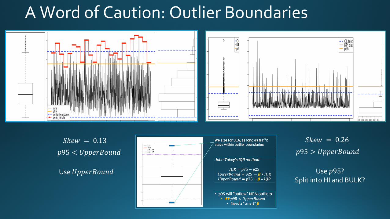
A Word of Caution: Outlier Boundaries

𝑆𝑘𝑒𝑤 = 0.13 𝑆𝑘𝑒𝑤 = 0.26

𝑝95 < 𝑈𝑝𝑝𝑒𝑟𝐵𝑜𝑢𝑛𝑑 𝑝95 > 𝑈𝑝𝑝𝑒𝑟𝐵𝑜𝑢𝑛𝑑

Use 𝑈𝑝𝑝𝑒𝑟𝐵𝑜𝑢𝑛𝑑 Use 𝑝95?Split into HI and BULK?

• There is no “one size fits all” approach.• There is no “one size fits all” statistic.• There are common principles:

• Aggregate before computing percentiles.• Use Outlier Boundaries:

• Performance & Capacity:• Accounts for the bulk of the data;• Distribution does not matter;

• Performance:• Easy to ID outliers;

• Capacity:• Sizing for Non-Outliers => less $

• Avoid Predefined Percentiles.


• Packets in flight; Packet Loss; % Utilization• Models:

• Correlations• Trends in Data

Coming Next

User Metrics:• throughput • latency• data loss• data loss & latency• latency & data loss

The Whirlpool of Metrics

For MonitoringReal metrics:• # of Packets in Flight • # of Packets in Queue or Lost

For Capacity Planning

Traditional Metrics in Planning:• 𝑇ℎ𝑟𝑜𝑢𝑔ℎ𝑝𝑢𝑡 [Gbps]• 𝐿𝑎𝑡𝑒𝑛𝑐𝑦hijklm

• 𝐿𝑎𝑡𝑒𝑛𝑐𝑦hinl = 𝑙𝑜𝑎𝑑𝑖𝑛𝑔||𝑟𝑒𝑎𝑠𝑠𝑒𝑚𝑏𝑙𝑦• Packets get queued and blocked.• Bits may be bursty while packets are smooth.

• Reverse statement is true as well.

• 𝐿𝑎𝑡𝑒𝑛𝑐𝑦hijklm = 𝑡𝑟𝑎𝑛𝑠𝑝𝑜𝑟𝑡 + 𝑞𝑢𝑒𝑢𝑒𝑖𝑛𝑔• Packets need capacity.

• Packet sizes vary => capacity [Gbps]

Example:320𝐺𝑏𝑝𝑠 = 26.7𝑀 ∗

1.5𝑘𝐵 ∗ 8 𝑏𝑖𝑡𝑠𝑠𝑒𝑐

320𝐺𝑏𝑝𝑠 = 10 ∗4𝐺𝑖𝐵 ∗ 8 𝑏𝑖𝑡𝑠

𝑠𝑒𝑐

Traditional Metrics for Monitoring:• % Utilization• Packet Loss Rate

Time, Rate, Count, and Utilization

𝑃𝑞 = 𝐸𝑟𝑙𝑎𝑛𝑔𝐶(𝑁, 𝐶)

Packet Queueing:

𝑃𝑏 = 𝐸𝑟𝑙𝑎𝑛𝑔𝐵(𝑁, 𝐶)

Packet Blocking:

2012 paper

𝑁 = 𝑃𝑃𝑆 ∗ 𝐿𝑎𝑡𝑒𝑛𝑐𝑦

𝐿𝑎𝑡𝑒𝑛𝑐𝑦 =12 ∗ 𝑅𝑇𝑇 + 𝑇��

𝑏𝑝𝑠 = 𝑃𝑃𝑆 ∗𝑏𝑖𝑡𝑠𝑝𝑎𝑐𝑘𝑒𝑡

𝐶 = 𝑚𝑎 𝑥 𝑃𝑃𝑆 ∗12 ∗ 𝑅𝑇𝑇

2006 paper(CPU centric)

• Utilization CAN BE useless• If the metric does not

reflect what it is used for.

links were utilized

near 100% [�h��h�] but

no packet drops

• There is no “one size fits all” approach.• There is no “one size fits all” statistic.• There are common principles:

• Aggregate before computing percentiles.• Use a statistic that accounts for the bulk of the data.

• Metric = what’s important to the BW user:• Quality of Service (QoS):

• Network Latency• Packets lost

• Models:• Trend in Data• Correlation• Time-Series Analysis

Coming Next

Trend in Data

Performance Monitoring:• Is this “normal” behavior?• Will this trend continue?• High values will be marked as outliers

• Are they?

Dealing with Trends

Option 1:• Fit in a linear regression• If it’s a good fit:

• Get distribution of residuals• Add p95 or outlier boundary of

residuals to regression line

Performance Monitoring:

This results in:

Option 1:Linear Regression -> Residualsallows us to detrend the data and deal with a stationary proxy…

… IFF:• Residuals are stationary• Residuals are normal• Residuals are homoscedastic

Performance Monitoring

If Residuals are Not Normal / Not Homoscedastic?

Linear Regressiondoes not work


Plan B: Directly Predict %-iles

Option 2 : Quantile Regression:rq (Demand ~ Time)


• Requires stationary trends• No need for homoscedasticity• No need for normality

Using Regression

1. Build regression for 𝐾𝑃𝐼 = 𝑓(𝐵𝑀); 2. TSA-forecast 𝑅𝑒𝑠𝑖𝑑𝑢𝑎𝑙𝑠;3. Predict 𝐾𝑃𝐼(𝐵𝑀|m ∗);4. Combine with forecast of 𝑅𝑒𝑠𝑖𝑑𝑢𝑎𝑙𝑠

Capacity Planning:

Problems: 𝑅𝑒𝑠𝑖𝑑𝑢𝑎𝑙𝑠 = 𝑓(𝑡𝑖𝑚𝑒)𝐼𝑛𝑡𝑒𝑟𝑐𝑒𝑝𝑡 = 𝑓(𝑡𝑖𝑚𝑒)

Using Quantile Regression Capacity Planning:

Great for most use cases

• No need for homoscedasticity• No need for normality• Works for correlated Time Series• Requires stationary trends• Old and New have same weight

Quantile Regression in Performance Monitoring

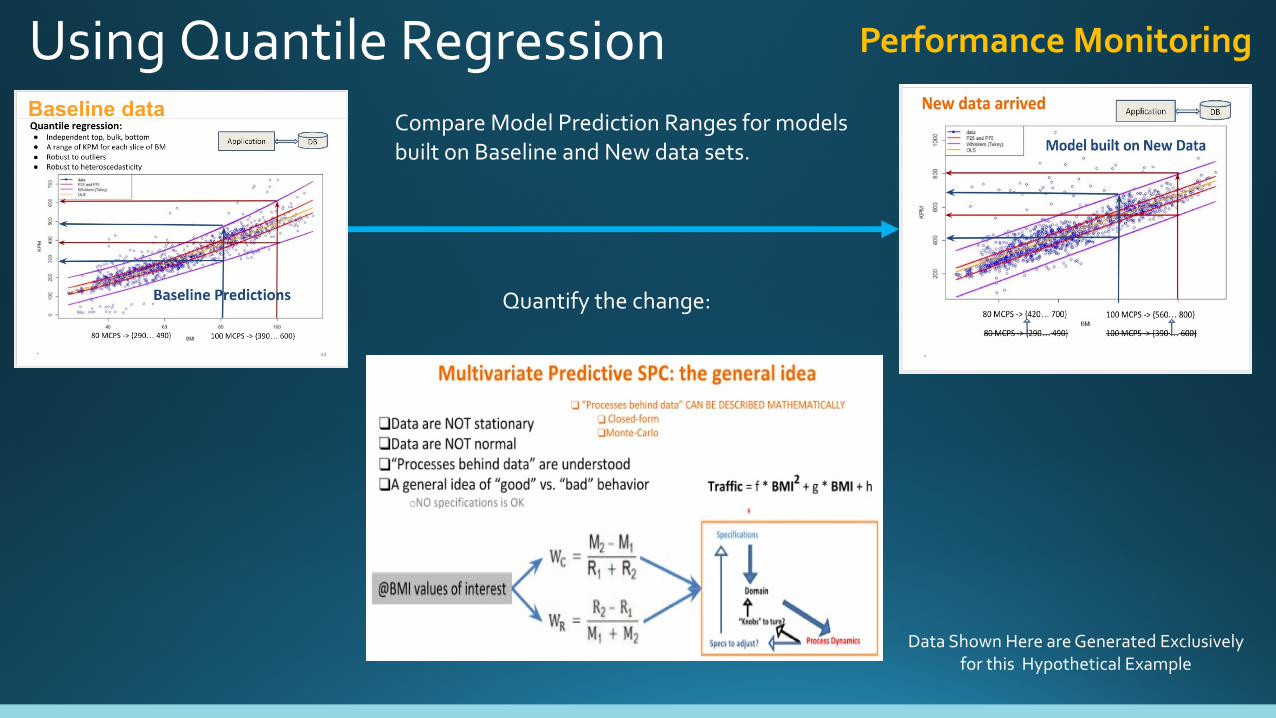
Using Quantile Regression Performance Monitoring

Compare Model Prediction Ranges for models built on Baseline and New data sets.

Quantify the change:

Baseline data

Data Shown Here are Generated Exclusively for this Hypothetical Example

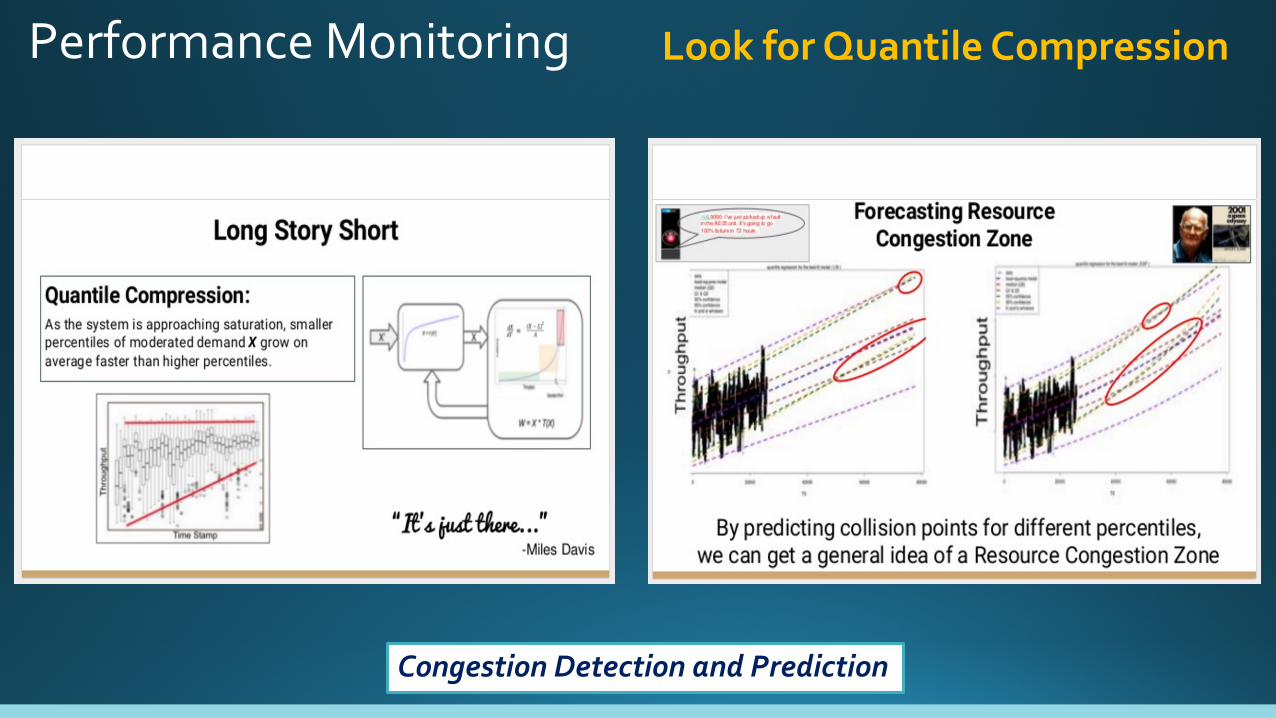
Performance Monitoring Look for Quantile Compression

Congestion Detection and Prediction

Time Series Analysis

Using Time Series Analysis

ETS (Error, Trend, Seasonality) Decomposition

For Performance Monitoring:

1. Fit a Forecasting (ETS) Model2. Get residuals3. Identify & Interpret Outliers in Residuals

4. Interpolate (or Predict) Outliers5. Re-fit Forecasting Model6. Predict Using the Fitted model

For Capacity Planning:

TSA Forecasting

Autoregressive(ARIMA) || ETS (EWMA) Forecasting

1. Fit a Forecasting Model2. Get residuals3. Identify Outliers4. Interpolate (or Predict) Outliers5. Re-fit Forecasting Model6. Predict Using the Fitted model

Issues / Problems / Challenges

How can we account for these variabilities?

• Underlying services have their own plans:• Growth• Deprecation• Relocation

• Supporting infrastructure has its own lifecycle:• New Product Introduction• Implementation and Growth• Depreciation• Tech Refresh

• Topologies and policies change in time• Change in policies and topology can lead to

changes in demand

Possible Solutions: Flow Level

1. Bottom-Up:• Forecast each service individually; • Follow up with Monte-Carlo aggregation

𝑆𝑣𝑐1

𝑆𝑣𝑐2

𝑆𝑣𝑐3

Possible Problem:Different prediction intervals not indicative of different data variability

Advantages:• Each service’s trend and variability is accounted for.• Each service’s growth plans are easy to account for.

𝐹𝑙𝑜𝑤1

1. Bottom-Up:Forecast each service individually; follow up with Monte-Carlo aggregation

Possible Problem:Different prediction intervals not indicative of different data variability


𝑆𝑣𝑐1

𝑆𝑣𝑐2

𝑆𝑣𝑐3

2. Top-Down:• Forecast the flow.• Get Distribution of each component’s weight in the flow.• Compute each component’s demand forecast

Possible Problems:Component Weights can drift in timeInteraction and Contention => “unknown unknown”


Solutions:Estimate Component WeightsAccount for Quantile Compression

𝑆𝑣𝑐1

𝑆𝑣𝑐2

𝑆𝑣𝑐3

𝑆𝑣𝑐3 𝑆𝑣𝑐2

𝑆𝑣𝑐1

Flow-Level TSA Forecasting

Autoregressive(ARIMA) || ETS (EWMA) Forecasting

1. Fit a Forecasting Model2. Get residuals3. Identify Outliers4. Interpolate (or Predict) Outliers5. Re-fit Forecasting Model6. Predict Using the Fitted model

For Capacity Planning:• TSA is NOT the Whole Story:

• Business Growth is not accounted for

Flow-Level Top-Down Stochastic Problem

Problem: 1. Flow composition varies from day to day.2. Flow composition also varies within a day.3. Old components may not be relevant anymore. 4. New components may not have enough history.

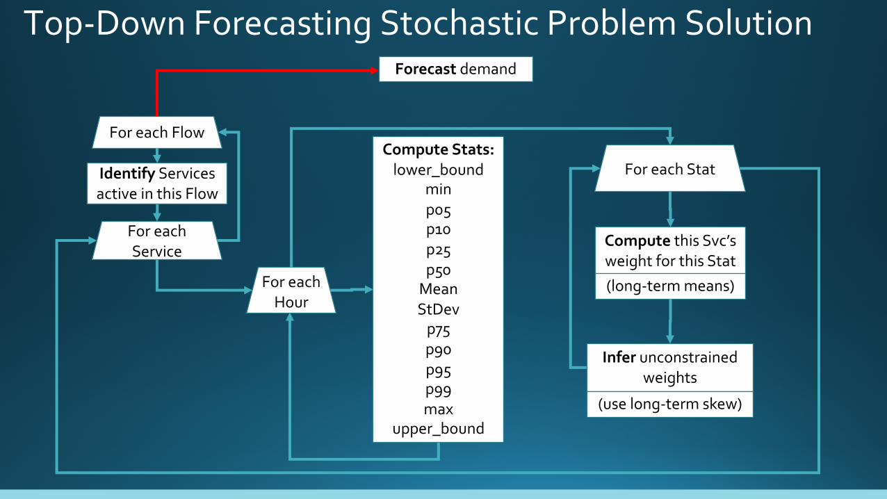
Top-Down Forecasting Stochastic Problem Solution

For each Flow

Forecast demand

(next 2 slides)

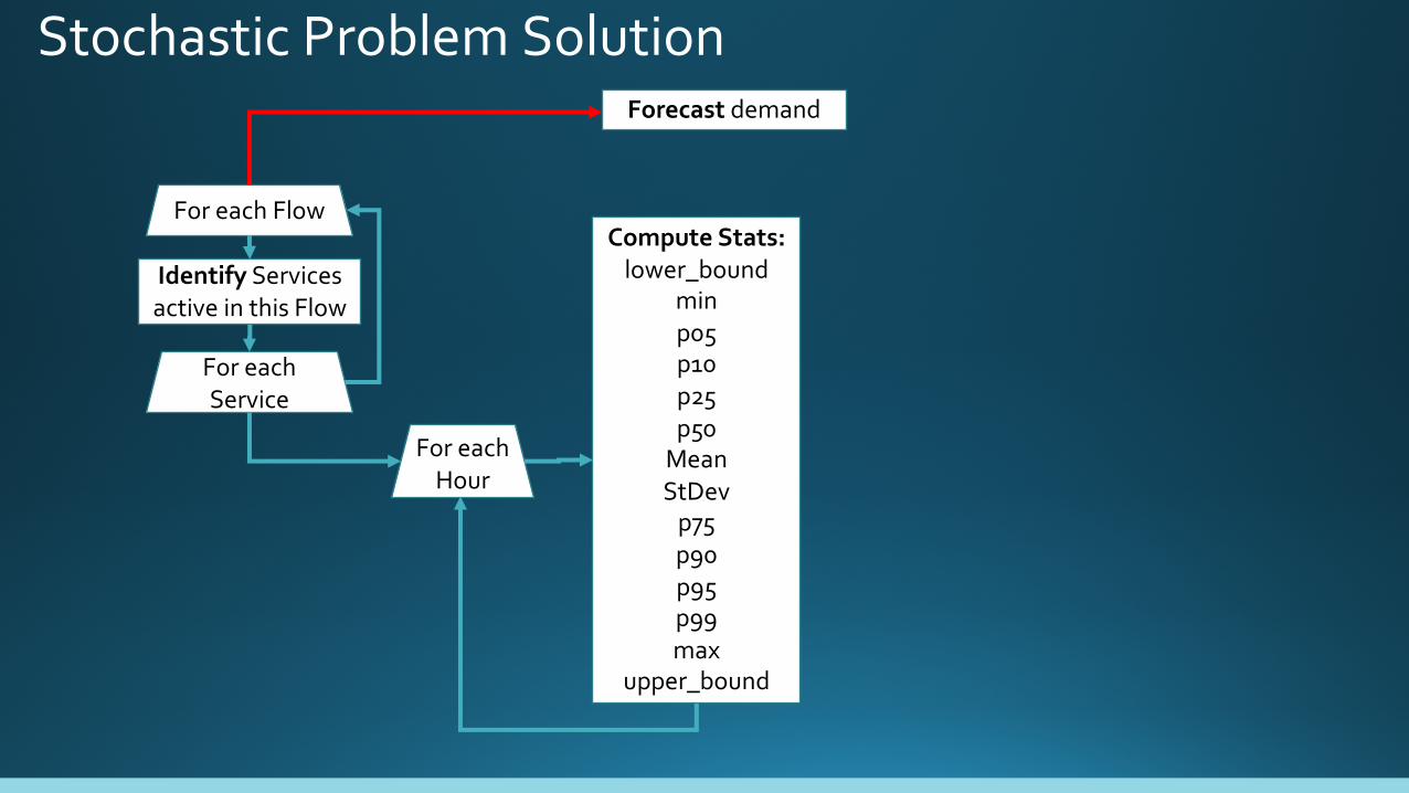
Stochastic Problem Solution

For each Flow

For each Service

Identify Services active in this Flow

Compute Stats:lower_bound

minp05p10p25p50

MeanStDev

p75p90p95p99max

upper_bound

For each Hour

Forecast demand

For each Flow

For each Service



minp05p10p25p50

MeanStDev

p75p90p95p99max

upper_bound

For each Hour

Compute this Svc’s weight for this Stat

For each Stat

(long-term means)

Infer unconstrained weights

(use long-term skew)

Forecast demand

Top-Down Forecasting Stochastic Problem Solution

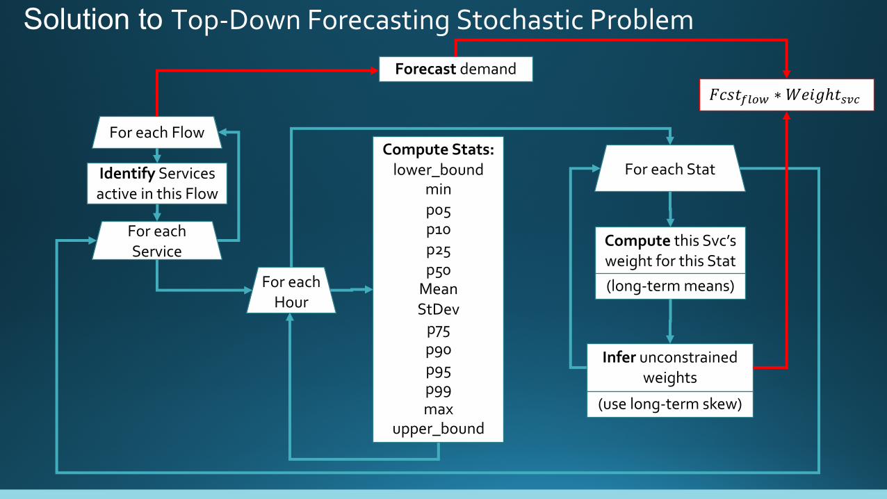
For each Flow

For each Service



minp05p10p25p50

MeanStDev

p75p90p95p99max

upper_bound

For each Hour

Compute this Svc’s weight for this Stat

For each Stat

(long-term means)

Infer unconstrained weights

(use long-term skew)

Forecast demand

𝐹𝑐𝑠𝑡�� ∗ 𝑊𝑒𝑖𝑔ℎ𝑡��j

Solution to Top-Down Forecasting Stochastic Problem

This Solves Most of the Problems• Underlying services have their own plans :

• Growth • Deprecation• Relocation

• USE PER-SERVICE DEPENDENCIES• Supporting infrastructure has its own lifecycle:

• New Product Introduction• Implementation and Growth• Depreciation• Tech Refresh

• USE PER-SERVICE /PER-FLOW DEPENDENCIES• Topologies and policies change in time

• Change in policies and topology can lead to changes in demand

• USE DUMMY VARIABLES

Now we can account for these variabilities!

Usefulness depends on:• Aggregation of Data

• StatMuxing?• Peak Hour?• Hourly Stats?

• Forecast Demand based on the Model• Bottoms-Up

• 𝑇𝑟𝑎𝑓𝑓𝑖𝑐 ∗ 𝑄𝑜𝑆 Drives 𝐷𝐶𝐿𝑜𝑎𝑑 Drives 𝑆𝑝𝑎𝑐𝑒&𝑃𝑜𝑤𝑒𝑟• Account for QoS in Demand Forecasting

• Plan for SLO

• DO NOT Assume Anything!

• Especially about Shapes of Distributions.

• Mean and Variance are Overrated!

• So is 𝑝95!

• Use Outlier Boundaries (“fences”)

• Size Systems for “would-be-unbounded” forecasts

• DO Use Entire Distribution to be Proactive

[email protected] / [email protected]@fb.com

All data in this presentation are generated solely for illustration purposesSelect images and formulae are provided with permission from Facebook

Capacity PlanningIs the number of Gbps on a constrained system indicative of demand?Is it right to forecast upper bound of traffic on a constrained system?

• Use 𝑝25, 𝑝50, and 𝑝75 to compute the 𝑆𝑘𝑒𝑤

• Forecast 𝑝25 and 𝑝50

• Use the 𝑆𝑘𝑒𝑤 to infer forecast of 𝑝75��j��m�iG�l�• Compute the forecast of 𝑈𝑝𝑝𝑒𝑟𝐵𝑜𝑢𝑛𝑑

Resource Constraint =>Quantile Compression =>

Underforecasting the load =>Undersizing the resource

Account for Quantile Compression

What is Quantile Compression?

Engineering

Performance OR Capacity #CMGimPACt2016