Maximizing network interruption in wireless

International Journal of Computer Networks & Communications (IJCNC) Vol.7, No.2, March 2015

DOI : 10.5121/ijcnc.2015.7209 103

MAXIMIZING NETWORK INTERRUPTION IN WIRELESS

SENSOR NETWORK: AN INTRUDER’S PERSPECTIVE

Mohammad Mahfuzul Islam1, Fariha Tasmin Jaigirdar2 and Mohammad Manzurul Islam3

1Department of Computer Science and Engineering, Bangladesh University of Engineering and Technology (BUET), Dhaka, Bangladesh

2Department of Computer Science and Engineering, Bangladesh University of Engineering and Technology (BUET), Dhaka, Bangladesh

3Faculty of Engineering and IT, University of Technology (UTS), Sydney, Australia

ABSTRACT With the colossal growth of wireless sensor networks (WSNs) in different applications starting from home automation to military affairs, the pressure on ensuring security in such a network is paramount. Considering the security challenges, it is really a hard-hitting effort to develop a secured WSN system. Moreover, as the information technology is getting popular, the intruders are also planning new ideas to break the system security, to harm the network and to make the system quality down with the target of taking the control of the network to corrupt it or to get benefits from it anyway. The intruders corrupt the system only when the security breaking cost (SBC) is lower compared with the benefits they attained or the harm it can make to others. In this paper, the authors define the term “maximizing network interruption problem” and propose a technique, called the grid point approximation algorithm, to estimate the SBC of a multi-hop WSN so that it can be made tougher for an intruder to break the system security. It is assumed that the intruder has the complete picture of the entire network. The technique is designed from the intruder’s point of view for completely jamming all the sensor nodes in the network through placing jammers or malicious nodes strategically and at the same time keeping the number of jammer nodes to minimum or near minimum. To the best of the authors’ knowledge, there is no work proposed so far of the same kind. Experimental results with the changes of the different network parameters show that the proposed algorithm is able to provide excellent performances to achieve the targets. KEYWORDS Wireless sensor network, Maximizing network interruption problem, Grid point approximation algorithm, Security breaking cost, Step-size. 1.INTRODUCTION

A wireless sensor network (WSN) is a wireless network consisting of distributed autonomous devices, called sensors, to cooperatively monitor physical or environmental conditions, such as temperature, vibration, pressure, motion or pollutants at different locations [1]. With the tremendous growing trend of computing and communication technologies, nowadays, WSNs are contentedly used in different applications ranging from home monitoring and automation to ocean and wildlife monitoring, industrial process monitoring, traffic control, healthcare applications, building safety and earthquake monitoring to many military applications [1]. The network can work both in a friendly environment as well as in an unfriendly or hostile environment to collect and to operate with sensitive data [2]. However, the wireless media are susceptible to easy access


104

by the intruders especially when data is transmitted through it from sensor devices having very poor computing facilities for protection. The signals in these media can also be interrupted easily through jamming or creating obstacles for the sensors to operate in a regular manner. By obliterating the regular operational activities of the network or by stealing sensitive data an intruder can readily get benefits or may cause harm to the targets. Therefore, ensuring the security during data gathering and transmission in WSN is highly imperative besides keeping up the smooth operation of the network. Ensuring proper security in a WSN is very difficult, if not impossible, because it is hard to implement sophisticated security algorithms within the tiny sensors. Moreover, the batteries stored inside the sensors supply very limited power and are died out quickly. Nevertheless, charging the battery in a sensor under deployment is intricate, if not impossible in many cases. The processing speed of a sensor device is also very limited to run complex methodologies. Therefore, implementing any effective security algorithms inside a sensor to protect its signals from the intruders is difficult and an intruder can easily attack a sensor node or damage its signals whenever it can arrive in a location where the sensors are within its transmission boundary. If the sensors in a WSN are deployed in close proximity, then a few numbers of intruders can spoil the network operation. Hence, deployment strategies used for WSN plays a vital role in ensuring both the operational and the data security of the network. No system in this universe is fully secured. As broadcasting is an inherent phenomenon in WSNs, wireless networks are vulnerable to maintain its security and unable to tackle most of the attacks like overhearing [3], jamming [4], malicious association and denial of service (DoS) [5]. Overhearing allows intruders to capture the target messages without changing the original transmitted from the sender when the signal is within the communication range of the intruders, i.e., the intruders are placed within the communication range of the sender. Nevertheless, Jamming deliberately uses its own radio noise or signals to disrupt the communication of signals from other targeted devices. The attack having the highest impact is called DoS, in which a malicious node disrupts the communication of signals among other nodes using various means and making the destination unreachable. In all of the above cases, the intruders target to make more harms to the system or to gain more profits from it utilizing its minimum possible budget. If a vicious activity made by an intruder costs more than the profit gained or the cost of harms enforced to others, then attacker must not choose such an activity for its misdeed. The attackers always explore the way to break the security of the system spending minimum amount of efforts or cost, which is termed as the security breaking cost (SBC) in this paper. A high-quality security ensuring algorithm, therefore, shall need to estimate the minimum SBC required for the intruders to make the algorithm robust. Maximizing network interruption problem (MIP) is the strategy to explore how maximum harms can be made to opponents or how maximum profits can be gained by an intruder through utilizing minimum resources, i.e., minimum SBC. MIP is an NP-hard problem [6] as the solution is a decision problem where optimal utilization of resources is to be made for ensuring the maximum harms or profits gained. This paper, for the first time to the best knowledge of the authors, proposes a low SBC based greedy solution to the MIP by using the grid approximation technique. The scheme is designed from the intruder’s perspective and assumed that the intruder has the complete picture of the entire network. The network deployment area is divided into smaller units through placing gridlines horizontally and vertically and then deployment of the malicious nodes are carried out strategically at the grid intersection points which best suits for making more harms to the networks or gaining more benefits from it at the lower cost. The scheme either corrupts the operation of entire WSN or overhears signals communicated within the region while keeping the number of malicious nodes to a minimum or near minimum.


105

Though the grid approximation technique is designed from the trespassers' perspective to make more harm in network operation or to get more benefits by analyzing the signals transmitted within the network, the concept it bears is very suitable for ensuring high level securities for the systems. Some of the practical target-oriented applications of the proposed scheme are as follows: (1) to measure the network security immunity power through simulating the proposed scheme on it; (2) to jog the memory of the proposed scheme while designing a new secured deployment strategy for WSN so that the SBC of the proposed network to be set up become higher; (3) to make the communication topology more complicated for the sniffers to overhear packets in view of the thoughts presented in the proposed scheme. The proposed grid approximation scheme can also be applied for quick data gathering inside the WSN coverage area, cost effective deployment of chargers for connectionless inductive remote charging, maximizing destruction to the opponents in the battlefield with minimum resources, earthquake monitoring with message passing and saving of scarce battery powers available in tiny sensors by keeping more nodes in sleeping mode. The rest of the paper is organized as follows. Section 2 describes the state-of-arts relating to the coverage problems which are not the same but constitutes related literatures required for presenting the novelty of the MIP and the proposed solution. The details of the strategies used in the proposed grid approximation technique and related algorithms are presented in Section 3. Section 4 presents experimental setups, simulation results and its comparative analysis under the variations of tuning parameters for proper investigations. Finally, some concluding remarks and future research directions are presented in Section 5. 2. LITERATURE REVIEW Monitoring is one of the key applications for WSN through which a target space or some objects are kept in close observation to ensure the proper protection of them from misdeeds or malfunctioning. In most applications, a number of sensors are deployed densely in an enclosed or a limited area to inspect whether some events take place in that specific zone or not. The coverage problem [7] is used to represent the processes where a specific area, or points or a boundary is monitored by deploying a number of sensors at multiple points. Nevertheless, a single monitoring device is deployed in the schemes commonly named as the minimum enclosing circle (MEC) [12] where the processes find the minimum coverage distance required for the device for monitoring all objects in a cram place. All of above mentioned techniques, having objectives, missions and methodologies different from the grid approximation technique; hold on important principles that are detailed below for defining the novelty and concepts of the proposed scheme. 2.1. The Coverage Problem The coverage problem [7] defines the problem of finding suitable techniques for monitoring/tracking a given place or its border lines or the objects lies inside the place using the possible minimum resources. The main goal of the coverage problem is to monitor each target in the physical space of interest within the sensing range by at least one sensor. Depending on the type of the targets, the coverage problem is divided into three classes—the area coverage, the point or target coverage and the barrier or path coverage [10]. Many works [7][9][10][11] have been proposed to explore the appropriate solutions for the different types of coverage problems. The basic principle of each type of the coverage problems is detailed below.


106

2.1.1. The Area Coverage Problem The area coverage problem monitors or covers the entire area of a given network with the goal of leaving no point in the target area unattained by the observer [7]. Figure 1 shows the scenario of an area coverage problem where each points within the square-shaped area ABCD is monitored or tracked by deploying a number of sensor nodes at different location inside the area.

Figure 1. Example of the area coverage problem

Most of the schemes solving the area coverage problem deploy sensors or monitoring devices randomly and use different techniques [7][8][9][13] to select some of them (as indicated by filled circles in Figure 1) for monitoring the location while keeping the rest in inactive, i.e., in sleeping mode (as indicated by unfilled circle) to reduce the wastage of scarce energy. In the coverage configuration protocol (CCP) [8], one of the prominent area coverage methods, the authors propose the k-coverage algorithm where each location within the particular area is covered by at least k sensors while keeping the maximum number of sensor nodes deployed in sleeping mode. If any case an active node goes out of energy, i.e., die out, a sleeping node becomes active to cover the uncovered zone and some mutations are performed between the active and the sleeping nodes to ensure the coverage of the entire area. The main problem of the CCP scheme is its time and space complexity as it has to solve NP-hard problem to select the required nodes that can guarantee the coverage of entire monitoring area under observation while keeping the number of active sensors to the minimum. The well-known optimal geographical density control (OGDC) scheme proposed by H. Zhang et. al. [9] addresses the problem using the greedy approach [14]. The first node, in the OGDC scheme, is selected randomly and the next one is selected which is the closest to the point located at the distance from the first one. The remaining nodes are selected repeating the process of taking the closest one to the point which is on the line perpendicular to the line connecting the positions of two previously selected sensors and situated at the distance of from the intersection point of two circles representing coverage. Selecting the node in such a directional way still has higher computational and time complexities. Nevertheless, the algorithm requiring the knowledge of the sensors' locations or directional information is difficult to implement. A solution to this problem is proposed in [17], where each sensor needs only to know the distances between adjacent nodes within its transmission range and their sensing radii. The authors in the paper design a polynomial-time distributed algorithm which mutates the activeness of sensors, maintaining a sequence on remaining energy, in every time slot in order to maximize the network lifetime. The upper bound of the network life-time and deviation in this algorithm from the upper bound has also been studied in this research paper. All of the schemes representing the solutions to the area coverage problem are designed to monitor a specific area under the observation by activating the sensors that are deployed


107

randomly in past. No such mechanism deploys nodes/sensors in real time using explorative way to corrupt or monitor devices located at some predefined points (rather than monitoring the entire area) besides maintaining the number of deployments to the minimum. 2.1.2. The Point or Target Coverage Problem The point or target coverage problem is a special case of area coverage problem in which, instead of inspecting all points in a specific area, a limited number of immobile devices or points of interest are monitored or tracked by activating required sensor devices from those deployed previous in a random manner [7][10]. Figure 2 represents the problem where the six targets are monitored by the three sensor nodes selected from the previous random deployments.

Figure 2. Example of the point coverage problem The maximum set cover approximation scheme [11] explores for all the minimum sets of sensors, selected from the previous random deployments and each of the sets is able to uniquely monitor or track all the targets. The NP-hard problem for selecting the minimum number of sensors covering all targets is solved by the greedy approach where the sensor covering the maximum number of targets within its transmission range is selected first. The scheme then selects one set of sensors containing the minimum number of elements for monitoring/tracking the targets so that the energy efficiency is prevailed. If any member of the selected set is died out, then set becomes unable to keep an eye on all the targets and, hence, the scheme chooses next set for monitoring. Moreover, common sensors are not always able to connect directly with the central node due to their limited ranges in asymmetrical wireless networks. Therefore, in [15] A. Rostami et al. utilize super nodes that have more energy, processing power and a wider range of communication. It does connectivity and transmits data to the base station, nevertheless, it is not possible for all simple nodes to connect to the super nodes directly and they transmit data through other nodes. The authors present an energy aware routing algorithm considering the energy of relay nodes to choose and transmit data and increase the lifetime of the network. Although this is a better solution for increasing network lifetime, but is dependent on those particular super nodes. So a round basis algorithm proves to be efficient in this manner. In [16] the authors propose a gravitational emulation local search algorithm (GELS) as a strategy to select optimal sensors. The goal of this algorithm is to increase network lifetime by optimization and reducing power consumption and increasing monitoring network efficiency. At first for each executive round in network, a number of sensors are activated to monitor all the targets. To solve the problem of optimal sensor the authors consider three matrixes, distance matrix, initial velocity matrix and time matrix. In this paper the energy and distances of a sensor node is calculated with different factors for gaining the mass and using the law of gravity different solutions are examined and finally from the solutions the optimal one is considered.


108

All the point or target coverage schemes select monitoring devices from those sensors pre-deployed randomly to inspect a limited number of points or targets and none of them are designed for explorative deployments of observers to corrupt or making harms to all the nodes in an existing network. The monitoring network is therefore based on the selection of nodes pre-existed, not superimposing another network with the vision of making harm to all nodes of the network already installed. 2.2. Minimum Enclosing Circle (MEC) The minimum enclosing circle (MEC) [12] is a mathematical problem for determining a circle having the smallest radius but containing all target points from a given set in the Euclidean plane [19]. The method is used to find out the location for placing a monitoring device and its required coverage distance to keep an eye on targeted region/objects or to find out a location for placing a shared facility. MEC can also be used to solve the "bomb problem" where the circle radius is used for determining the minimum explorative capacity of the bomb and the center of the circle is the best place to drop the bomb for maximizing the level of destructions to the enemies. The algorithm proposed in [12] constructs a number of possible circles and select the one with the smallest radius that encompasses all the target points. Y. Lin et.al. [18] present another MEC implementation technique where deployment is performed by placing the multiple base stations or sinks each at the geometric center of a cluster in a WSN to maximize network lifetime in case of both the one-hop and the multi-hop communication. MIP differs from the MEC such that there is only one observant or malicious node in the later whose coverage radius varies arbitrarily depending on the transmission power level and the deployment environment. Nevertheless, MIP uses multiple vigilant or malicious nodes with the same or different coverage distance and deployment is performed by selecting the best location for them. 3. PROPOSED NETWORK INTERRUPTION MAXIMIZATION SCHEME MIP explores for a cost-effective and efficient strategy to deploy malicious nodes in a coverage zone such that all the active participants working in that zone become corrupted or failed to perform its activities. Figure 3 illustrates that at least three malicious nodes (represented by red circles) are necessary to corrupt the transmission of 13 (thirteen) sensors nodes (A to M), represented by blue circles. A blind deployment strategy, however, performs random deployment within the target zone to corrupt the sensor devices and requires 13 malicious nodes in worse-case to corrupt the entire network.

Figure 3. Jamming a sensor network


109

The malicious nodes are usually more powerful than the sensor nodes deployed because complex speed and memory intensive applications are required to be executed inside such devices. From an intruders perspective, it is not realistic to spend equal or more resources to make harm to others by making the entire network inactive. The main objective of this paper is to explore the best locations for deployment of malicious nodes while making the entire target zone tarnished by the minimum number. The optimum solution to this problem is an NP-hard [6] problem. The authors of this paper propose a heuristic solution named "the grid approximation scheme" to solve the proposed MIP problem. The scheme divides the entire deployment location into small squares through placing imaginary gridlines to explore points for malevolent node deployments at the locations nearest to the optimal. The scheme is detailed below. 3.1. The Grid Approximation Scheme The grid approximation scheme at first defines a square space that encompasses the entire WSN and places a number of horizontal and vertical gridlines on it to divide the space into small square precincts. Let a two-dimensional field of size D×D square precincts includes a WSN consisting of N sensor nodes deployed as shown in Figure 4. It is assumed that all the malicious nodes deployed are homogeneous and have the same transmission distance, denoted by R. Therefore, to jam a wireless sensor node v, a jamming node j must be placed so that ||v, j|| <= R, i.e., the distance between v and j is required to be less than or equal to R. The authors in this paper assume that the intruder has the full knowledge about the network topology as each sensor has a low-power Global Positioning System (GPS) [20]. If GPS is not available, the distance between neighbouring nodes can be estimated on the basis of incoming signal strengths.

Figure 4. Network architecture The proposed grid approximation scheme places the malicious nodes at the grid points only. For ensuring maximum destruction, the scheme uses the greedy approach to find out the mostly dense region centred at a grid point in order to place the first malicious node. Stepping ahead, the strategy removes those sensor nodes that are already jammed by the malicious node placed at the selected junction. The process repeats recursively to add more malicious nodes at the appropriate grid points until all the sensors nodes are removed or covered being within the transmission ranges of them. The strategy stops on finding out the minimum or near minimum number of malicious or jamming nodes required to corrupt all the sensor nodes in the network.

(1,1)

(D,0)

---------- (0,0)

(2,1) (3,1)

(1,0) (2,0) (3,0)

(0,1) (D,1)

(1,2) (2,2) (3,2) (0,2)

(1,3) (2,3) (3,3)

----------

(D,2)

(D,3) (0,3)

(1,4) (2,4) (3,4) (D,4)

(D,D)

----------

----------

---------- (0,4)

(1,D) (2,D) (3,D)


110

Let Si(xi,yi), 1 ≤ i ≤ N be a sensor node in the WSN deployed randomly at the location (xi, yi), where 0 ≤ xi, yi ≤ D and G(m, n) be the grid points produced by the scheme within the target region such that m, n {0, 1, 2, 3, 4, ....., D}. Therefore, the distance between a sensor node Si(xi,yi) and a grid point G(m, n) is calculated using the Euclidian distance as follows,

22 )()(,,, nymxnmGyxSdis iiiii

(1) Eq. (1) is the generalized distance calculating equation which is used for finding out the prospective member nodes of each grid points. Thus the malicious node placed at a grid point disrupts the communications of all sensor member nodes of that grid point. Throughout the procedure, the strategy maintains a table with only those grid points having at least one member node, i.e., sensor node within the R distance. The densest area in the grid structure is determined by the reference of the grid point having the highest number of member nodes. If is the

distance of the sensor Si(xi,yi) from the point G(m, n), then

nmGyxSdisk iiimni ,,, (2)

The number of member nodes in a grid point G(m, n) is the count of distances having value

less than R. (3)

A table is generated for all the grid points G(m, n) such . The first candidate

grid point for placing the malicious node is chosen as the one containing the maximum

number of member nodes K.

)max( mnKK (4) After getting the first malicious node position, , the strategy deletes all the member nodes of

the grid point , i.e., all the sensor nodes covered by the malicious node placed at the grid point

from the table. The table is then revised by deleting the row of the table for the grid point

and reducing the number of member nodes for the grid points G(p, q) by deleting

the sensor nodes that are also members of where,

and (5)

The grid approximation technique reapplies the same greedy method to the revised table to find out the next near optimum position for placing the next malicious node until the table becomes empty.


111

3.2. An Example To clearly portray the operation procedure of grid approximation technique, the authors of this paper use a 6×6 sized grid structure as an example, indicating in Figure 5. Each grid point is marked by G (m, n), where (m, n), 0 ≤ m, n ≤ 5 represents the point in the grid. The grid approximation scheme investigates for the sensor nodes deployed within the grid region to be interrupted by the malicious node with coverage distance R placed in each grid point.

Figure 5. A 6×6 sized grid structure

The WSN attempt to be interrupted as shown in this example contains 11 sensor nodes deployed in scattered manner within the region as depicted in Figure 6. Each blue circle has the radius R as shown in the figure and represents the region that can be covered by individual malicious node placed at the grid point, i.e., the centre of the circle. Table 1 shows the implementation/simulation scenario where each grid point that is able to cover at least one sensor is listed in along with the identity number of the sensors, such as only sensor node n1 is within the communication range from grid point G (1, 1), sensor nodes n1, n2 and n3 are within the communication range from the grid point G (1, 2). The third column represents the number of nodes that can be covered by the corresponding grid point. It is observed from the table that a specific sensor node may be covered from more than one malicious node, i.e., grid points. The scheme then explores for the minimum number of locations for placing malicious node using the concept of the minimum set cover problem [22]. The greedy approach first looks for the grid point such that placing a malicious node in that point covers the maximum number of sensors. In Table 1, placing a malicious node at grid point G (3, 3) will covered maximum number of six sensors represented by n*, where * = {6, 7, 8, 9, 10, 11}. So, this is the position for the first malicious node deployment guaranteeing the maximum number of transmission blockade in the network.

Figure 6. Deploying the sensor nodes over the network

(0,1) (1,1) (2,1)

(3,1) (4,1) (5,1)

(0,2) (1,2) (2,2) (3,2) (4,2) (5,2)

(0,3) (1,3) (2,3) (3,3) (4,3) (5,3)

(0,4) (1,4) (2,4) (3,4) (4,4) (5,4)

(0,5) (1,5) (2,5) (3,5) (4,5) (5,5)


112

After exploring the location for the first malevolent node, the table is reduced through applying the Pruning Strategy and location for the next malevolent node is identified. The process repeated until all the sensor nodes are interrupted by at least one of the malicious agents.

Table 1. Grid point’s member nodes and total node count.

Grid points Covered nodes Total G(1,1) n1 1 G(1,2) n1, n2, n3 3 G(2,2) n1, n3 2 G(2,3) n6, n7,n8 3 G(2,4) n8, n9 2 G(3,1) n4, n5 2 G(3,2) n4, n5 2 G(3,3) n6, n7, n8, n9, n10, n11 6 G(3,4) n8, n9, n10, n11, 4 G(4,2) n5 1 G(4,3) n10, n11 2

. 3.2.1. Pruning Strategy The pruning strategy of grid approximation technique each time when applied removes all entries in the row containing the grid point, say G(m, n), identified for placing the next malicious nodes. The strategy then accounts the sensor nodes listed against G (m, n) in the deleted row of the table that are the candidates to be covered by the malevolent node placed at the said grid point. The accounted sensors nodes are then deleted from each row of the table represented by the grid points G (m±R, n±R) where appears and the total count for the corresponding row is recalculated. In example, the first identified grid point is G (3, 3). So, the row containing G (3, 3) is deleted and sensor nodes n* in the row are accounted. In the second step, the accounted sensor nodes are deleted from the rows represented by G (3±1, 3±1), i.e., G (2, 2), G (2, 3), G (2, 4), G (3, 2), G (4, 2), G (4, 3), and G (3, 4) and the total count for these rows {2, 3, 2, 2, 1, 2, 4} is changed to {2, 0, 0, 2, 1, 0, 0}. After the modification, the new table is ready to be used for finding out the next location for the malicious nodes and the pruning strategy to be reapplied again. Both the strategies are repeated until the table becomes empty, i.e., all the sensor nodes are covered by the malicious agents deployed. Finally, the strategy terminates by finding a list of three grid points represented by G (3, 3), G (1, 2) and G (3, 1). 3.3. Malicious Node Placement Algorithm This section demonstrates the proposed grid approximation algorithm and describes its different steps to clearly depict all iterations. The different parameters used in the algorithm are the number of sensor nodes (NN), the transmission range (R), the maximum dimension limit of the grid structure (XMAX, YMAX) and the step-size of the grid (∆). The algorithm assumes that the sensor nodes are already deployed randomly in a two dimensional grid structure. Step 1 of the algorithm represents the random placement of the sensor nodes. Upon placing all the sensor nodes, distances are calculated from each sensor node to each grid point for


113

finding out every grid point’s member set, as indicated in step 5. Step 1 to step 10 formulate the table containing the grid points that have sensor nodes within the transmission zone. At the beginning of the algorithm, all the sensor nodes are considered as unaffected nodes, representing in step 11. Step 12 starts with a while loop that continues till all the sensor nodes are jammed by the intruders assuring the condition num_unaffected to be greater than 0. Step 14 to step 19 searches for all the grid point entries in the table in order to find out the highest sensor node covering the grid-point, where to place the intruder. Step 20 updates the num_unaffected array by deleting the already jammed sensor nodes. Step 21 to step 30 calculate the grid points that have already covered sensor nodes within their transmission range for deleting already covered entries of sensor nodes from the table. Step 31 to step 33 determine the number of intruders (along with their positions) needed for jamming all the sensor nodes by guaranteeing the num_unaffected value to be zero.

Algorithm Grid (NN, R, XMAX,YMAX, ∆) Input: Transmission range, R, Number of sensor nodes, NN, Maximum dimension in x-axes, XMAX, Maximum dimension in y-axes, YMAX, Step-size, ∆. Output: Deployment position of the intruders and the number of intruders. /*num_unaffected=number of unaffected nodes, pCount= number of grid point entries in the table, hNPcount= the value of highest number of sensor node covered by a grid point, nCount= sensor node count in the table, HighestPointNode= the point that has the maximum number of sensor nodes in its transmission range.*/ 1. Sensor nodes are deployed randomly over the deployment area, i.e.; XMAX×YMAX 2. for i := 0 to YMAX step ∆ 3. for j := 0 to XMAX step ∆ 4. for k := 0 to NN 5. if distance from all the grid points to all the sensor nodes ≤ R 6. those grid points are inserted in the table /*Here only those grid points are inserted in the table who have sensor nodes in their transmission range, i.e., the grid points that does not has any neighbour, not need to include in the table.*/ 7. endif 8. endfor 9. endfor 10. endfor 11. num_unaffected := NN 12. while(num_unaffected > 0) 13. hNPcount := 0 14. for i := 0 to pCount /*Checking for all the grid point entries in the table to find out the point that has maximum number of sensor nodes in its transmission range*/ 15. if nCount[i] > hNPcount 16. hNPcount := nCount [i] 17. HighestPointNode := i 18. endif 19. endfor /*Here the position of first malicious node is found and also the number of sensor nodes it covers.*/ 20. num_unaffected := num_unaffected-hNPcount /*Now the algorithm checks for other grid point entries within the upper and


114

lower bound of the transmission range of the HighestPointNode to determine whether they have those sensor nodes within their transmission range, R, as they have already been covered and that is why, need to be deleted.*/ 21. for j :=0 to pCount 22. if j :≠ HighestPointNode 23. Check for those grid points that resides between the transmission range of 24. HighestPoint Node, i.e., within ±R of HighestPointNode 25. for k := 0 to nCount [j] 26. if redundant node exist, delete all of them from the entries and update the table 27. endif 28. endfor 29. endif 30. endfor 31. nCount [HighestPointNode] := 1 32. Show all the malicious node position 33. Endwhile

3.4. Complexity Analysis The efficiency of the algorithm is to be analysed by calculating the time and space complexity. The space complexity of the proposed algorithm is proportionate to the number of grid points. For estimating the time complexity, the authors assume the grid size G = D×D, number of grid points

NG = number of sensors = NS, cost for calculating distance = CD, cost of each

comparison = CG and transmission range of the malicious nodes = R, ∆ is the step size. In the first iteration, distances of all sensor nodes from each grid point are calculated and then find the point that covers the maximum number of nodes within its transmission range. Thus the first iteration has two steps. In step 1.1, the time complexity of finding the distances of all sensor nodes from a given grid point is NSCD and hence for all grid point it becomes NGNSCD. In step 1.2, number of comparison for finding the point that cover the maximum number of nodes is NGNS and total comparison cost is NGNSCG. So, the total time-complexity for finding the grid point covering the maximum sensor nodes is NGNSCD + NGNSCG, i.e., NGNS (CD+CG). The second and consecutive iteration ensures that all the sensor nodes are jammed. The computational complexity at this stage is calculated by dividing the algorithm in different steps as shown below: Step 2.1: Upon finding the point (p, q) that holds the maximum number of nodes in its transmission range, the algorithm has to adjust which points need to be searched next. The adjustment points are (p ± r, q ± r). So, the total points to be searched are (2r×2r-1) = (4r2-1), where, r = ceiling (R/∆). Step 2.2: Then the sensor nodes that have already been covered by the chosen grid point are deleted from the list and require NDNS comparisons, where ND is the number of sensor nodes covered by the grid point and deleted from the list. So, the time complexity for the iteration is (4r2-1) NDNSCG.


115

Step 2.3: For finding rest of the grid points, the algorithm repeats the process for NS-ND sensor nodes and (NG-1) grid points. If the sensor nodes are distributed randomly and equally spaced within the region, then the number of grid points, p, chosen for intruders can be estimated as . So the time

complexity is estimated as,

Solving the equation, the complexity of the algorithm is found as,

Therefore, the total time complexity found for the algorithm is,

.

4. EXPERIMENTAL SETUP This section illustrates the experimental arrangement to evaluate the performance of the grid approximation technique. Different considering factors are added here for clear understanding the network scenario as well as the different network parameters ranges. 4.1. Simulation Setup The authors have developed a simulation software in Java environment using the discrete event simulation toolkit, SimJava [23]. The simulations were carried out in an Intel Xeon processor with 2GB RAM. The environment, number of sensors, step size for placing grids and other simulation parameters were chosen carefully to ensure that the real environment is to be reflected through simulation. 4.1.1. Environmental Setting To set up the simulation environment, a 2D space having size of D×D is used and N sensor nodes deployed in that space. The number of nodes, N is changed to several values for examining the effects of the algorithm. The dimensional length, D also varied into different ranges for analyzing the effects of the algorithm on different space size, i.e., from small to large network. 4.1.2. Changing Step-size While considering the grid structure for any simulation, a major concern is to decide the distance or the step size used for the gridlines. As the proposed grid approximation technique deploys the malicious nodes in the grid points only, measuring step size, i.e., the distance between two nearest grid points is a major feature for designing the algorithm. The goal of the scheme is not only finding the better locations for placing the malicious nodes and ensuring the number to the


116

minimum or the nearer, but also emphasizing on the processing steps and time complexity, which is by any case not desirable to be amplified.

Figure 7. Maximum distance between two grid points Let AB = BC = CD= AD = X be the step size used for a particular empirical analysis for placing malicious nodes as shown in Figure 7. As the covering distance of a malicious node is R, the distance between two nearest malicious nodes must be at most 2R to ensure the sensor nodes in any location within the region will be under the coverage of the malicious node. So, for the maximum step size, the diagonal distance between two consecutive grid points is BD = 2R. From Pythagoras theorem [21], the relationship can be written as, , i.e.,

. The maximum step size, X, therefore can be obtain as R. The minimum distance of the step-size can be any distance greater than or equal to zero and hence, 0 < X ≤ R.

At step-size X, there will be NG = grid points within the region . . 4.1.3. Simulation Parameters The different parameters used for simulation environment are the transmission range R, i.e., a malicious node’s covering range of receiving and transmitting signals, number of sensor nodes N, total networking area or dimension, D and step-size, Δ. To increase the accuracy of simulation results, the outcome of the simulation has been obtained at least five times for the same snapshots of the experimental environments and parameters and then the average is taken. Different values of the changing parameters used in simulation are listed in Table 2.

Table 2. Different values of network parameters.

Parameters Values Transmission Range, R

5, 8, 10, 20, 40

Number of Nodes, N

70,100,150,200,300,500

Dimension, D 100, 150, 200, 300 Step-size, Δ 1 to R


117

4.2. Simulation Result and Comparative Analysis Different simulation results and their comparative analysis are added in this section for determining the proposed algorithm’s efficiency. By varying the network parameters, Figure 8, 9 and 10 show three line charts that estimate the number of intruders needed to destroy all the deployed sensor nodes in the network.

Figure 8. Results by changing transmission range and dimension

Transmission range, R is the most important one among the three network parameters, when sensor node covering is the prime issue. Figure 8 shows the arrangement of the first scenario by keeping the number of nodes value fixed 200 and changes the value of transmission range, R (5, 8 and 10) and network topology, D(100×100, 200×200 and 300×300). It can be observed from Figure 8 that as the transmission range increases, the number of intruders needed to jam the network decreases accordingly. The reason is, with the increasing value of transmission range, more nodes can be within the range of the grid points (i.e., by placing a malicious at that point all the sensors that are within the transmission range of that point can be jammed easily) and number of intruders is lessening accordingly. Here, the intruder required is minimum for the highest valued transmission range, i.e., 10 in every charts and lowest for the low valued transmission range, 5. The second scenario adjusts the value of dimension and number of nodes, while transmission range remains fixed, 40. For establishing sophisticated applications of wireless sensor networks, another important parameter of a network is number of nodes, N. Figure 9 and 10 shows that, in most of the cases, as number of nodes increase the number of intruders require increase accordingly. This is because, with higher number of nodes, more malicious nodes are necessary to embrace them meeting the corresponding criteria. On a contrary, an exception is marked in Figure 9. That is, while the algorithm moves from number of nodes 100 to 150, the number of intruders needed is decreased. The reason is very obvious. The sensor nodes are deployed randomly over the networking region. As a result, if the nodes are placed in close proximity to all other nodes, it is possible to find out the most dense region of the sensors in a scenario that occurs in Figure 9. Thus, this region can be covered by minimum number of nodes easily rather than sparsely deployed sensors. In spite of such exceptional scenario, in most of the cases, as the number of nodes increases, the number of intruders required also increases accordingly which easily can be seen from Figure 9 and 10. By fixing the dimension or network topology, D, 300×300 the last scenario of experimental analysis deals with changing the other two parameters. In a large area,


118

where nodes are placed randomly it is normally happens that they are placed in a scattered manner and that is why more intruders are required to cover all the nodes in the network. Figure 8 and 9 shows that in most of the cases, as the dimension increase the number of intruders needed increase accordingly.

Figure 9. Results by changing dimension and number of nodes

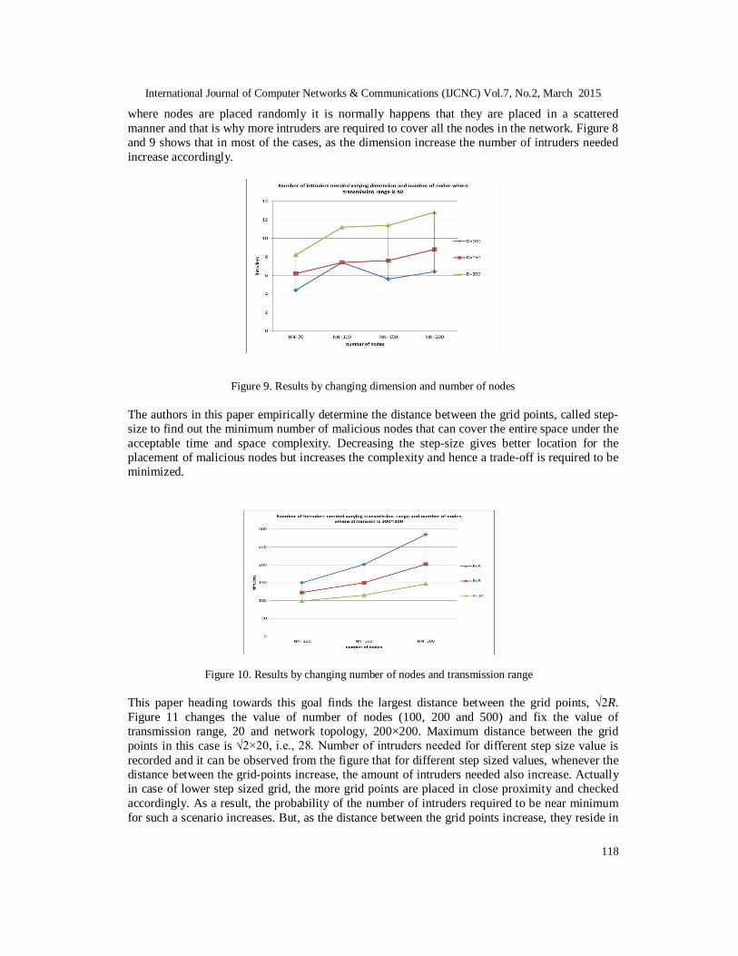
The authors in this paper empirically determine the distance between the grid points, called step-size to find out the minimum number of malicious nodes that can cover the entire space under the acceptable time and space complexity. Decreasing the step-size gives better location for the placement of malicious nodes but increases the complexity and hence a trade-off is required to be minimized.

Figure 10. Results by changing number of nodes and transmission range

This paper heading towards this goal finds the largest distance between the grid points, √2R. Figure 11 changes the value of number of nodes (100, 200 and 500) and fix the value of transmission range, 20 and network topology, 200×200. Maximum distance between the grid points in this case is √2×20, i.e., 28. Number of intruders needed for different step size value is recorded and it can be observed from the figure that for different step sized values, whenever the distance between the grid-points increase, the amount of intruders needed also increase. Actually in case of lower step sized grid, the more grid points are placed in close proximity and checked accordingly. As a result, the probability of the number of intruders required to be near minimum for such a scenario increases. But, as the distance between the grid points increase, they reside in


119

far space than previous placement. Therefore, the number of intruders required to embrace them increase accordingly.

Figure 11. : Results for different step size value by changing number of nodes while keeping dimension and transmission range fixed

Though escalating step size of the grid structure increases the desired number of intruders, the authors in this paper analysis the processing steps of the proposed architecture here that would be helpful for taking decisions on choosing the correct value of the step size. Figure 12 shows the processing step values for different step size and also indicate how processing step values change with the changing values of the step size. Considering a two-dimensional network structure of 100×100 and the transmission range, 20, for unit distanced step size, the processing step is 10000, where as for the maximum distanced step size, 28, the processing step value drop off to13, which is too minor in comparison to the previous value.

Figure 12. : Processing steps required for different step sized value 5. CONCLUSIONS AND FUTURE WORKS Designing a secured network or making the network durable against its security breakdown is a burning issue in developing an appropriate structure of a wireless network. This paper deals with the security issue from an intruder’s point of view with the goal of finding those regions where by placing malicious nodes maximum interruption is possible and finally searches for the minimum or near minimum number of intruders or malicious nodes needed to completely jam or destroy all the sensor nodes in the network. The authors in this paper describe these as a problem called “the maximizing network interruption problem” and find the solution of it by deriving an efficient and


120

cost-effective grid approximation algorithm. The proposed algorithm implies some bounds on how difficult it is for an intruder to launch an operational attack on the communication or signal passing of the network with a minimum power budget. Thus the security strength of a network is head to head comparable with the proposed strategy. By developing an algorithm from the intruders' perspective, the authors proposes an excellent means for security engineers to make their network robust by making the security breaking cost higher so that the intruders do not get any benefits through breaking the system security. The algorithm can further be enhanced by redesigning it for distributed environment and for mobile sensor devices under the reduced complexity and the reduced power consumption. REFERENCES [1] J Yick, B Mukherjee and D Ghosal, Wireless Sensor Network Survey, Computer Networks, 52, 2292-

2330 (2008). [2] C –Y Chong and S P Kumar, Sensor Networks: Evolution, Opportunities and Challenges,

Proceedings of IEEE, 1247-1256 (2003). [3] P Basu and J Redi, Effect of Overhearing Transmissions on Energy Efficiency in Dense Sensor

Networks, Proceedings of third International Symposium on Information Processing in Sensor Networks, 196-204(2004).

[4] W Xu, K Ma, W Trappe and Y Zhang, Jamming Sensor Networks: Attack and Defense Strategies, Network, IEEE, 20( 3), 41-47, May-June (2006).

[5] Z Cao, X Zhou, M Xu, Z Chen, J Hu and L Tang, Enhancing Base Station Security against DoS Attacks in Wireless Sensor Networks, IEEE International Conference on Wireless communications, networking and Mobile Computing (WiCOM), 22-24 Sept 2006.

[6] NP-Hard Problem, http://www.princeton.edu/~achaney/tmve/wiki100k/docs/NP-hard.html, Accessed 30 Mar 2014.

[7] M Cardei and J Wu, Coverage in Wireless Sensor Networks, Handbook of Sensor Networks, CRC Press(2004).

[8] X Wang, G Xing,Y Zhang,C Lu,R Pless and C Gill, Integrated Coverage and Connectivity Configuration in Wireless Sensor Networks,ACM Transactions on Sensor Networks, 36-72(2005).

[9] H Zhang, and J C Hou, Maintaining Sensing Coverage and Connectivity in Large Sensor Networks,International Journal of Ad Hoc & Sensor Wireless Networks, 89-124(2005).

[10] G J Fan and S Jin, Coverage Problem in Wireless Sensor Network: A Survey, Journal of Networks, 319-329(2010).

[11] M Cardei, M Thai, Y Li and W Wu, Energy-efficient target coverage in wireless sensor networks, 24th Annual Joint Conference of the IEEE Computer and Communications Societies, 1976-1984, 13-17 Mar 2005.

[12] Minimum Enclosing Circle Problem, http://www.cs.mcgill.ca/~cs507/projects/1998/jacob/problem.htnl, Accessed 27 Jun 2011.

[13] M. Marengoni, A. B. Draper, A. Hanson, and R. Sitaraman, A System to Place Observers on Polyhedral Terrain in Polynomial Time, Image and Vision Computing, 18, 773-780 (2000).

[14] K Jain, M Mahdian & A Saberi, A New Greedy Approach for Facility Location Problems, Proceedings of the 34th annual ACM symposium on theory of computing, 731-740 (2002).

[15] A S Rostami, M R Tanhatalab, H M Berneti, Novel Algorithm of Energy-Aware in Asymmetric Wireless Sensor Networks Routing for In-point Coverage, International Conference on Computational Intelligence and Communication Networks(CICN), 308-313, 27-28 Nov 2010.

[16] A Bagrezai, S V A -D Makki and A S Rostami, A New Energy Consumption Algorithm with Active Sensor Selection using GELS in Target Coverage WSN, International Journal of Computer Science Issues (IJCSI), 10(1) (2013).

[17] G S Kasbekar, Y Bejerano and S Sarkar,Lifetime and Coverage Guarantees through Distributed Coordinate-free Sensor Activation, IEEE/ACM transaction in Networking, 19(2), 470-483 (2011).

[18] Y Lin, Q Wu, X Cai, X Du and K Kwon, On Deployment of Multiple Base Stations for Energy-Efficient Communication in Wireless Sensor Networks, International journal of distributed sensor networks, 2010, (2010).

http://www.princeton.edu/~achaney/tmve/wiki100k/docs/NP-hard.html,

http://www.cs.mcgill.ca/~cs507/projects/1998/jacob/problem.htnl,


121

[19] P Winter, An Algorithm for the Steiner Problem in the Euclidian Plane, Networks an International Journal, 15 (3), 323-345 (1985).

[20] A E Rabbany, Introduction to GPS: The Global Positioning System, Library of Congress Cataloguing in Publication Data (2002).

[21] Pythagoras Theorem, http://www.mathsisfun.com/pythagoras.html, 5 Jan 2011. [22] P Zhang, R-L Wang, C-G Wu and K Okazaki, An Effective Algorithm for the Minimum Set Cover

Problem, International Conference on Machine learning and Cybernetics, 3032-3035, 13-16 Aug 2006.

[23] A Sobeih, W –P Chen, J C Hou, L –C Kung, N Li, H Lim, H –Y Tyan and H Zhang, J-Sim: A Simulation Environment for Wireless Sensor Networks, Proceedings of the 38th annual simulation symposium (ANSS’05), IEEE, 175-187, 4-6 Apr 2005.

Authors Dr. Mohammad Mahfuzul Islam has completed his Bsc. and Msc. Engineering in Computer Science and Engineering from Bangladesh University of Engineering and Technology (BUET). Mahfuz has achieved his Phd degree from Monash University, Australia. He is working in Buet in the Dept. of Computer Science and Engineering as a Professor and Head of the department. His research area is wireless cellular network. He has a number of conferences and journal in this field. Dr. Islam is the President of Bangladesh Computer Society (BCS). He is also member of IEEE. Fariha Tasmin Jaigirdar was born in Chittagong, Bangladesh at 9th May, 1983. Fariha has completed Bsc. Engineering in Computer Science and Engineering from Chittagong University of Engineering and Technology (CUET) in. Her Msc. Engineering in Computer Science and Engineering has been completed from Bangladesh University of Engineering and Technology (BUET) in 2011 with the submission of thesis entitled “Maximizing Network Interruption: An Intruder’s Perspective”.At present she is working in Daffodil International University as an Assistant Professor in the dept. of Computer Science and Engineering. Her research interest includes wireless network and digital signal processing. She has attended three conferences of ICCIT, Bangladesh, 2009 to 2011. She has more than five publications in different journals also. She has two poster papers. Recently she is working on different applications of Wireless Sensor Network. Mohammad Manzurul Islam received his M.Sc. degree in Information Technology with major in Internetworking from University of Technology Sydney (UTS) in 2013. He obtained his B.Sc. degree in Computer Science and Information Technology from Islamic University of Technology (IUT) in 2005. He started his career as a Lecturer of Computer Science and Engineering department in Stamford University Bangladesh. At the same time, he was the Legal Main Contact, Curriculum Lead and Instructor of Cisco Local Academy. Currently he is working as an Assistant Professor of Computer Science and Engineering department in Stamford University Bangladesh. His research interests include networking, network security and wireless sensor network.

http://www.mathsisfun.com/pythagoras.html,