Embed Size (px)
Citation preview

CHAPMAN & HALL/CRCA CRC Press Company
Boca Raton London New York Washington, D.C.
Simulations forRadar SystemsDesign
Bassem R. Mahafza, Ph.D.Decibel Research, Inc.Huntsville, Alabama
Atef Z. ElsherbeniProfessorElectrical Engineering DepartmentThe University of MississippiOxford, Mississippi
© 2004 by Chapman & Hall/CRC CRC Press LLC

This book contains information obtained from authentic and highly regarded sources. Reprinted materialis quoted with permission, and sources are indicated. A wide variety of references are listed. Reasonableefforts have been made to publish reliable data and information, but the author and the publisher cannotassume responsibility for the validity of all materials or for the consequences of their use.
Neither this book nor any part may be reproduced or transmitted in any form or by any means, electronicor mechanical, including photocopying, microfilming, and recording, or by any information storage orretrieval system, without prior permission in writing from the publisher.
The consent of CRC Press LLC does not extend to copying for general distribution, for promotion, forcreating new works, or for resale. Specific permission must be obtained in writing from CRC Press LLCfor such copying.
Direct all inquiries to CRC Press LLC, 2000 N.W. Corporate Blvd., Boca Raton, Florida 33431.
Trademark Notice:
Product or corporate names may be trademarks or registered trademarks, and areused only for identification and explanation, without intent to infringe.
Visit the CRC Press Web site at www.crcpress.com
© 2004 by Chapman & Hall/CRC CRC Press LLC
No claim to original U.S. Government worksInternational Standard Book Number 1-58488-392-8Library of Congress Catalog Number 2003065397
Printed in the United States of America 1 2 3 4 5 6 7 8 9 0Printed on acid-free paper
Library of Congress Cataloging-in-Publication Data
Mahafza, Bassem R.MATLAB simulations for radar systems design / Bassem R. Mahafza, Atef
Z. Elsherbenip. cm.
Includes bibliographical references and index.ISBN 1-58488-392-8 (alk. paper)1. Radar–Computer simulation. 2. Radar–Equipment and
supplies–Design and construction–Data processing. 3. MATLAB. I.Elsherbeni, Atef Z. II. TitleTK6585.M34 2003621.3848
′
01
′
13—dc22 2003065397
C3928_disclaimer Page 1 Wednesday, November 5, 2003 1:36 PM
© 2004 by Chapman & Hall/CRC CRC Press LLC

© 200
To: My wife and four sons;
Wayne and Shirley;
and
in the memory of my parents
Bassem R. Mahafza
To: My wife and children;
my mother;
and
in the memory of my father
Atef Z. Elsherbeni
4 by Chapman & Hall/CRC CRC Press LLC
© 200
Preface
The emphasis of MATLAB Simulations for Radar Systems Design is on radar systems design. However, a strong presentation of the theory is provided so that the reader will be equipped with the necessary background to perform radar systems analysis. The organization of this book is intended to teach a conceptual design process of radars and related trade-off analysis and calcula-tions. It is intended to serve as an engineering reference for radar engineers working in the field of radar systems. The MATLAB®1 code provided in this book is designed to provide the user with hands-on experience in radar sys-tems, analysis and design.
A radar design case study is introduced in Chapter 1 and carried throughout the text, where the authors view of how to design this radar is detailed and analyzed. Trade off analyses and calculations are performed. Additionally, sev-eral mini design case studies are scattered throughout the book.
MATLAB Simulations for Radar Systems Design is divided into two parts: Part I provides a comprehensive description of radar systems, analyses and design. A design case study, which is carried throughout the text, is introduced in Chapter 1. In each chapter the authors view of how to design the case-study radar is presented based on the theory covered up to that point in the book. As the material coverage progresses through the book, and new theory is dis-cussed, the design case-study requirements are changed and/or updated, and of course the design level of complexity is also increased. This design process is supported by a comprehensive set of MATLAB 6 simulations developed for this purpose. This part will serve as a valuable tool to students and radar engi-neers in helping them understand radar systems, design process. This includes 1) learning how to go about selecting different radar parameters to meet the design requirements; 2) performing detailed trade-off analysis in the context of radar sizing, modes of operations, frequency selection, waveforms and signal processing; 3) establishing and developing loss and error budgets associated with the design; and 4) generating an in-depth understanding of radar opera-tions and design philosophy. Additionally, Part I includes several mini design case studies pertinent to different chapters in order to help enhance understand-ing of radar design in the context of the material presented in different chap-ters.
Part II includes few chapters that cover specialized radar topics, some of which is authored and/or coauthored by other experts in the field. The material
1. MATLAB is a registered trademark of the The MathWorks, Inc. For product infor-mation, please contact: The MathWorks, Inc., 3 Apple Hill Drive, Natick, MA 01760-2098 USA. Web: www.mathworks.com.
4 by Chapman & Hall/CRC CRC Press LLC
© 200
included in Part II is intended to further enhance the understanding of radar system analysis by providing detailed and comprehensive coverage of these radar related topics. For this purpose, MATLAB 6 code has also been devel-oped and made available.
All MATLAB programs and functions provided in this book can be down-loaded from the CRC Press Web site (www.crcpress.com). For this purpose, follow this procedure: 1) from your Web browser type http://www.crc-press.com, 2) click on Electronic Products, 3) click on Download & Updates, and finally 4) follow instructions of how to download a certain set of code off that Web page. Furthermore, this MATLAB code can also be down-loaded from The MathWorks Web site by following these steps: 1) from your Web browser type: http://mathworks.com/matlabcentral/fileexchange/, 2) place the curser on Companion Software for Books and click on Communi-cations. The MATLAB functions and programs developed in this book include all forms of the radar equation: pulse compression, stretch processing, matched filter, probability of detection calculations with all Swerling models, High Range Resolution (HRR), stepped frequency waveform analysis, ghk tracking filter, Kalman filter, phased array antennas, clutter calculations, radar ambiguity functions, ECM, chaff, and many more.
Chapter 1 describes the most common terms used in radar systems, such as range, range resolution, and Doppler frequency. This chapter develops the radar range equation. Finally, a radar design case study entitled MyRadar Design Case Study is introduced. Chapter 2 is intended to provide an over-view of the radar probability of detection calculations and related topics. Detection of fluctuating targets including Swerling I, II, III, and IV models is presented and analyzed. Coherent and non-coherent integration are also intro-duced. Cumulative probability of detection analysis is in this chapter. Visit 2 of the design case study MyRadar is introduced.
Chapter 3 reviews radar waveforms, including CW, pulsed, and LFM. High Range Resolution (HRR) waveforms and stepped frequency waveforms are also analyzed. The concept of the Matched Filter (MF) is introduced and ana-lyzed. Chapter 4 presents in detail the principles associated with the radar ambiguity function. This includes the ambiguity function for single pulse, Lin-ear Frequency Modulated pulses, train of unmodulated pulses, Barker codes, and PRN codes. Pulse compression is introduced in Chapter 5. Both the MF and the stretch processors are analyzed.
Chapter 6 contains treatment of the concepts of clutter. This includes both surface and volume clutter. Chapter 7 presents clutter mitigation using Moving Target Indicator (MTI). Delay line cancelers implementation to mitigate the effects of clutter is analyzed.
Chapter 8 presents detailed analysis of Phased Arrays. Linear arrays are investigated and detailed and MATLAB code is developed to calculate and plot
4 by Chapman & Hall/CRC CRC Press LLC
© 200
the associated array patterns. Planar arrays, with various grid configurations, are also presented.
Chapter 9 discusses target tracking radar systems. The first part of this chap-ter covers the subject of single target tracking. Topics such as sequential lob-ing, conical scan, monopulse, and range tracking are discussed in detail. The second part of this chapter introduces multiple target tracking techniques. Fixed gain tracking filters such as the and the filters are presented in detail. The concept of the Kalman filter is introduced. Special cases of the Kal-man filter are analyzed in depth.
Chapter 10 is coauthored with Mr. J. Michael Madewell from the US Army Space and Missile Defense Command, in Huntsville, Alabama. This chapter presents an overview of Electronic Counter Measures (ECM) techniques. Top-ics such as self screening and stand off jammers are presented. Radar chaff is also analyzed and a chaff mitigation technique for Ballistic Missile Defense (BMD) is introduced.
Chapter 11 is concerned with the Radar Cross Section (RCS). RCS depen-dency on aspect angle, frequency, and polarization is discussed. The target scattering matrix is developed. RCS formulas for many simple objects are pre-sented. Complex object RCS is discussed, and target fluctuation models are introduced. Chapter 12 is coauthored with Dr. Brian Smith from the US Army Aviation and Missile Command (AMCOM), Redstone Arsenal in Alabama. This chapter presents the topic of Tactical Synthetic Aperture Radar (SAR). The topics of this chapter include: SAR signal processing, SAR design consid-erations, and the SAR radar equation. Finally Chapter 13 presents an overview of signal processing.
Using the material presented in this book and the MATLAB code designed by the authors by any entity or person is strictly at will. The authors and the publisher are neither liable nor responsible for any material or non-material losses, loss of wages, personal or property damages of any kind, or for any other type of damages of any and all types that may be incurred by using this book.
Bassem R. MahafzaHuntsville, Alabama
July, 2003
Atef Z. ElsherbeniOxford, Mississippi
July, 2003
αβ αβγ
4 by Chapman & Hall/CRC CRC Press LLC

© 200
Acknowledgment
The authors first would like to thank God for giving us the endurance and perseverance to complete this work. Many thanks are due to our families who have given up and sacrificed many hours in order to allow us to complete this book. The authors would like to also thank all of our colleagues and friends for their support during the preparation of this book. Special thanks are due to Brian Smith, James Michael Madewell, Patrick Barker, David Hall, Mohamed Al-Sharkawy, and Matthew Inman who have coauthored and/or reviewed some of the material in this reference book.
4 by Chapman & Hall/CRC CRC Press LLC

© 200
Table of Contents
Preface Acknowledgment
PART I
Chapter 1 Introduction to Radar Basics
1.1. Radar Classifications 1.2. Range 1.3. Range Resolution 1.4. Doppler Frequency 1.5. The Radar Equation
1.5.1. Radar Reference Range 1.6. Search (Surveillance)
1.6.1. Mini Design Case Study 1.1 1.7. Pulse Integration
1.7.1. Coherent Integration 1.7.2. Non-Coherent Integration 1.7.3. Detection Range with Pulse Integration 1.7.4. Mini Design Case Study 1.2
1.8. Radar Losses 1.8.1. Transmit and Receive Losses 1.8.2. Antenna Pattern Loss and Scan Loss 1.8.3. Atmospheric Loss 1.8.4. Collapsing Loss 1.8.5. Processing Losses 1.8.6. Other Losses
1.9. MyRadar Design Case Study - Visit 1
4 by Chapman & Hall/CRC CRC Press LLC

© 200
1.9.1 Authors and Publisher Disclaimer 1.9.2. Problem Statement 1.9.3. A Design 1.9.4. A Design Alternative
1.10. MATLAB Program and Function Listings Listing 1.1. Function radar_eq.m Listing 1.2. Program fig1_12.m Listing 1.3. Program fig1_13.m Listing 1.4. Program ref_snr.m Listing 1.5. Function power_aperture.m Listing 1.6. Program fig1_16.m Listing 1.7. Program casestudy1_1.m Listing 1.8. Program fig1_19.m Listing 1.9. Program fig1_21.m Listing 1.10. Function pulse_integration.m Listing 1.11. Program myradarvisit1_1.m Listing 1.12. Program fig1_27.m
Appendix 1APulsed Radar
1A.1. Introduction 1A.2. Range and Doppler Ambiguities 1A.3. Resolving Range Ambiguity 1A.4. Resolving Doppler Ambiguity
Appendix 1BNoise Figure
Chapter 2Radar Detection
2.1. Detection in the Presence of Noise 2.2. Probability of False Alarm 2.3. Probability of Detection 2.4. Pulse Integration
2.4.1. Coherent Integration 2.4.2. Non-Coherent Integration 2.4.3. Mini Design Case Study 2.1
2.5. Detection of Fluctuating Targets 2.5.1. Threshold Selection
4 by Chapman & Hall/CRC CRC Press LLC
© 200
2.6. Probability of Detection Calculation 2.6.1. Detection of Swerling V Targets 2.6.2. Detection of Swerling I Targets 2.6.3. Detection of Swerling II Targets 2.6.4. Detection of Swerling III Targets 2.6.5. Detection of Swerling IV Targets
2.7. The Radar Equation Revisited 2.8. Cumulative Probability of Detection
2.8.1. Mini Design Case Study 2.2 2.9. Constant False Alarm Rate (CFAR)
2.9.1. Cell-Averaging CFAR (Single Pulse) 2.9.2. Cell-Averaging CFAR with Non-Coherent Integra-
tion 2.10. MyRadar Design Case Study - Visit 2
2.10.1. Problem Statement 2.10.2. A Design
2.10.2.1. Single Pulse (per Frame) Design Option 2.10.2.2. Non-Coherent Integration Design Option
2.11. MATLAB Program and Function Listings Listing 2.1. Program fig2_2.m Listing 2.2. Function que_func.m Listing 2.3. Program fig2_3.m Listing 2.4. Function marcumsq.m Listing 2.5. Program prob_snr1.m Listing 2.6. Program fig2_6a.m Listing 2.7. Function improv_fac.m Listing 2.8 Program fig2_6b.m Listing 2.9. Function incomplete_gamma.m Listing 2.10. Function factor.m Listing 2.11. Program fig2_7.m Listing 2.12. Function threshold.m Listing 2.13. Program fig2_8.m Listing 2.14. Function pd_swerling5.m Listing 2.15. Program fig2_9.m Listing 2.16. Function pd_swerling1.m Listing 2.17. Program fig2_10.m Listing 2.18. Program fig2_11ab.m Listing 2.19. Function pd_swerling2.m Listing 2.20. Program fig2_12.m Listing 2.21. Function pd_swerling3.m Listing 2.22. Program fig2_13.m Listing 2.23 Function pd_swerling4.m Listing 2.24. Program fig2_14.m
4 by Chapman & Hall/CRC CRC Press LLC
© 200
Listing 2.25. Function fluct_loss.m Listing 2.26. Program fig2_16.m Listing 2.27. Program myradar_visit2_1.m Listing 2.28. Program myradar_visit2_2.m Listing 2.29. Program fig2_21.m
Chapter 3Radar Waveforms
3.1. Low Pass, Band Pass Signals and Quadrature Components
3.2. The Analytic Signal 3.3. CW and Pulsed Waveforms 3.4. Linear Frequency Modulation Waveforms 3.5. High Range Resolution 3.6. Stepped Frequency Waveforms
3.6.1. Range Resolution and Range Ambiguityin SWF
3.6.2. Effect of Target Velocity 3.7. The Matched Filter 3.8. The Replica 3.9. Matched Filter Response to LFM Waveforms 3.10. Waveform Resolution and Ambiguity
3.10.1. Range Resolution 3.10.2. Doppler Resolution 3.10.3. Combined Range and Doppler Resolution
3.11. Myradar Design Case Study - Visit 3 3.11.1. Problem Statement 3.11.2. A Design
3.12. MATLAB Program and Function Listings Listing 3.1. Program fig3_7.m Listing 3.2. Program fig3_8.m Listing 3.3. Function hrr_profile.m Listing 3.4. Program fig3_17.m
Chapter 4The Radar Ambiguity Function
4.1. Introduction 4.2. Examples of the Ambiguity Function
4.2.1. Single Pulse Ambiguity Function 4.2.2. LFM Ambiguity Function
4 by Chapman & Hall/CRC CRC Press LLC

© 200
4.2.3. Coherent Pulse Train Ambiguity Function 4.3. Ambiguity Diagram Contours 4.4. Digital Coded Waveforms
4.4.1. Frequency Coding (Costas Codes) 4.4.2. Binary Phase Codes 4.4.3. Pseudo-Random (PRN) Codes
4.5. MyRadar Design Case Study - Visit 4 4.5.1. Problem Statement 4.5.2. A Design
4.6. MATLAB Program and Function Listings Listing 4.1. Function single_pulse_ambg.m Listing 4.2. Program fig4_2.m Listing 4.3. Program fig4_4.m Listing 4.4. Function lfm_ambg.m Listing 4.5. Program fig4_5.m Listing 4.6. Program fig4_6.m Listing 4.7. Function train_ambg.m Listing 4.8. Program fig4_8.m Listing 4.9. Function barker_ambg.m Listing 4.10. Function prn_ambg.m Listing 4.11. Program myradar_visit4.m
Chapter 5Pulse Compression
5.1. Time-Bandwidth Product 5.2. Radar Equation with Pulse Compression 5.3. LFM Pulse Compression
5.3.1. Correlation Processor 5.3.2. Stretch Processor 5.3.3. Distortion Due to Target Velocity
5.4. MyRadar Design Case Study - Visit 5 5.4.1. Problem Statement 5.4.2. A Design
5.5. MATLAB Program and Function Listings Listing 5.1. Program fig5_3.m Listing 5.2. Function matched_filter.m Listing 5.3. Function power_integer_2.m Listing 5.4. Function stretch.m Listing 5.5. Program fig5_14.m
4 by Chapman & Hall/CRC CRC Press LLC

© 200
Chapter 6Surface and Volume Clutter
6.1. Clutter Definition 6.2. Surface Clutter
6.2.1. Radar Equation for Area Clutter - Airborne Radar
6.6.2. Radar Equation for Area Clutter - Ground BasedRadar
6.3. Volume Clutter 6.3.1. Radar Equation for Volume Clutter
6.4. Clutter Statistical Models 6.5. MyRadar Design Case Study - Visit 6
6.5.1. Problem Statement 6.5.2. A Design
6.6. MATLAB Program and Function Listings Listing 6.1. Function clutter_rcs.m Listing 6.2. Program myradar_visit6.m
Chapter 7Moving Target Indicator (MTI) and Clutter Mitiga-tion
7.1. Clutter Spectrum 7.2. Moving Target Indicator (MTI) 7.3. Single Delay Line Canceler 7.4. Double Delay Line Canceler 7.5. Delay Lines with Feedback (Recursive Filters) 7.6. PRF Staggering 7.7. MTI Improvement Factor
7.7.1. Two-Pulse MTI Case 7.7.2. The General Case
7.8. MyRadar Design Case Study - Visit 7 7.8.1. Problem Statement 7.8.2. A Design
7.9. MATLAB Program and Function Listings Listing 7.1. Function single_canceler.m Listing 7.2. Function double_canceler.m Listing 7.3. Program fig7_9.m Listing 7.4. Program fig7_10.m Listing 7.5. Program fig7_11.m Listing 7.4. Program myradar_visit7.m
4 by Chapman & Hall/CRC CRC Press LLC
© 200
Chapter 8Phased Arrays
8.1. Directivity, Power Gain, and Effective Aperture 8.2. Near and Far Fields 8.3. General Arrays 8.4. Linear Arrays
8.4.1. Array Tapering 8.4.2. Computation of the Radiation Pattern via the DFT
8.5. Planar Arrays 8.6. Array Scan Loss 8.7. MyRadar Design Case Study - Visit 8
8.7.1. Problem Statement 8.7.2. A Design
8.8. MATLAB Program and Function Listings Listing 8.1. Program fig8_5.m Listing 8.2. Program fig8_7.m Listing 8.3. Function linear_array.m Listing 8.4. Program circular_array.m Listing 8.5. Function rect_array.m Listing 8.6. Function circ_array.m Listing 8.7. Function rec_to_circ.m Listing 8.8. Program fig8_53.m
Chapter 9 Target Tracking
Single Target Tracking9.1. Angle Tracking
9.1.1. Sequential Lobing9.1.2. Conical Scan
9.2. Amplitude Comparison Monopulse9.3. Phase Comparison Monopulse9.4. Range Tracking
Multiple Target Tracking9.5. Track-While-Scan (TWS)9.6. State Variable Representation of an LTI System 9.7. The LTI System of Interest 9.8. Fixed-Gain Tracking Filters
9.8.1. The Filter9.8.2. The Filter
αβαβγ
4 by Chapman & Hall/CRC CRC Press LLC

© 200
9.9. The Kalman Filter 9.9.1. The Singer -Kalman Filter9.9.2. Relationship between Kalman and
Filters 9.10. MyRadar Design Case Study - Visit 9
9.10.1. Problem Statement 9.10.2. A Design
9.11. MATLAB Program and Function Listings Listing 9.1. Function mono_pulse.m Listing 9.2. Function ghk_tracker.m Listing 9.3. Program fig9_21.m Listing 9.4. Function kalman_filter.m Listing 9.5. Program fig9_28.m Listing 9.6. Function maketraj.m Listing 9.7. Function addnoise.m Listing 9.8. Function kalfilt.m
PART II
Chapter 10Electronic Countermeasures (ECM)
10.1. Introduction 10.2. Jammers
10.2.1. Self-Screening Jammers (SSJ) 10.2.2. Stand-Off Jammers (SOJ)
10.3. Range Reduction Factor 10.4. Chaff
10.4.1. Multiple MTI Chaff Mitigation Technique 10.5. MATLAB Program and Function Listings
Listing 10.1. Function ssj_req.m Listing 10.2. Function sir.m Listing 10.3. Function burn_thru.m Listing 10.4. Function soj_req.m Listing 10.5. Function range_red_factor.m Listing 10.6. Program fig8_10.m
Chapter 11 Radar Cross Section (RCS)
11.1. RCS Definition 11.2. RCS Prediction Methods 11.3. Dependency on Aspect Angle and Frequency
αβγαβγ
4 by Chapman & Hall/CRC CRC Press LLC
© 200
11.4. RCS Dependency on Polarization 11.4.1. Polarization 11.4.2. Target Scattering Matrix
11.5 RCS of Simple Objects 11.5.1. Sphere 11.5.2. Ellipsoid 11.5.3. Circular Flat Plate 11.5.4. Truncated Cone (Frustum) 11.5.5. Cylinder 11.5.6. Rectangular Flat Plate 11.5.7. Triangular Flat Plate
11.6. Scattering From a Dielectric-Capped Wedge 11.6.1. Far Scattered Field 11.6.2. Plane Wave Excitation 11.6.3. Special Cases
11.7. RCS of Complex Objects 11.8. RCS Fluctuations and Statistical Models
11.8.1. RCS Statistical Models - Scintillation Models 11.9. MATLAB Program and Function Listings
Listing 11.1. Function rcs_aspect.m Listing 11.2. Function rcs_frequency.m Listing 11.3. Program example11_1.m Listing 11.4. Program rcs_sphere.m Listing 11.5. Function rcs_ellipsoid.m Listing 11.6. Program fig11_18a.m Listing 11.7. Function rcs_circ_plate.m Listing 11.8. Function rcs_frustum.m Listing 11.9. Function rcs_cylinder.m Listing 11.10. Function rcs_rect_plate.m Listing 11.11. Function rcs_isosceles.m Listing 11.12. Program Capped_WedgeTM.m Listing 11.13. Function DielCappedWedgeTM
Fields_LS.m Listing 11.14. Function
DielCappedWedgeTMFields_PW.m Listing 11.15. Function polardb.m Listing 11.16. Function dbesselj.m Listing 11.17. Function dbessely.m Listing 11.18. Function dbesselh.m Listing 11.19. Program rcs_cylinder_complex.m Listing 11.20. Program Swerling_models.m
4 by Chapman & Hall/CRC CRC Press LLC
© 200
Chapter 12 High Resolution Tactical Synthetic Aperture Radar (TSAR)
12.1. Introduction 12.2. Side Looking SAR Geometry 12.3. SAR Design Considerations 12.4. SAR Radar Equation 12.5. SAR Signal Processing 12.6. Side Looking SAR Doppler Processing 12.7. SAR Imaging Using Doppler Processing 12.8. Range Walk 12.9. A Three-Dimensional SAR Imaging Technique
12.9.1. Background 12.9.2. DFTSQM Operation and Signal Processing 12.9.3.Geometry for DFTSQM SAR Imaging 12.9.4. Slant Range Equation 12.9.5. Signal Synthesis 12.9.6. Electronic Processing 12.9.7. Derivation of Eq. (12.71) 12.9.8. Non-Zero Taylor Series Coefficients for the kth
Range Cell 12.10. MATLAB Programs and Functions
Listing 12.1. Program fig12_12-13.m
Chapter 13 Signal Processing
13.1. Signal and System Classifications 13.2. The Fourier Transform 13.3. The Fourier Series 13.4. Convolution and Correlation Integrals 13.5. Energy and Power Spectrum Densities 13.6. Random Variables 13.7. Multivariate Gaussian Distribution 13.8. Random Processes 13.9. Sampling Theorem13.10. The Z-Transform13.11. The Discrete Fourier Transform13.12. Discrete Power Spectrum 13.13. Windowing Techniques13.14. MATLAB Programs
Listing 13.1. Program figs13.m
4 by Chapman & Hall/CRC CRC Press LLC

© 200
Appendix 13A
Fourier Transform Table
Appendix 13B
Some Common Probability Densities
Appendix 13C
Z - Transform Table
Chapter 14 MATLAB Program and Function Name List
Bibliography
4 by Chapman & Hall/CRC CRC Press LLC
© 200
Chapter 1 Introduction to Radar Basics
1.1. Radar ClassificationsThe word radar is an abbreviation for RAdio Detection And Ranging. In
general, radar systems use modulated waveforms and directive antennas to transmit electromagnetic energy into a specific volume in space to search for targets. Objects (targets) within a search volume will reflect portions of this energy (radar returns or echoes) back to the radar. These echoes are then pro-cessed by the radar receiver to extract target information such as range, veloc-ity, angular position, and other target identifying characteristics.
Radars can be classified as ground based, airborne, spaceborne, or ship based radar systems. They can also be classified into numerous categories based on the specific radar characteristics, such as the frequency band, antenna type, and waveforms utilized. Another classification is concerned with the mission and/or the functionality of the radar. This includes: weather, acquisi-tion and search, tracking, track-while-scan, fire control, early warning, over the horizon, terrain following, and terrain avoidance radars. Phased array radars utilize phased array antennas, and are often called multifunction (multi-mode) radars. A phased array is a composite antenna formed from two or more basic radiators. Array antennas synthesize narrow directive beams that may be steered mechanically or electronically. Electronic steering is achieved by con-trolling the phase of the electric current feeding the array elements, and thus the name phased array is adopted.
Radars are most often classified by the types of waveforms they use, or by their operating frequency. Considering the waveforms first, radars can be Con-
4 by Chapman & Hall/CRC CRC Press LLC
© 200
tinuous Wave (CW) or Pulsed Radars (PR).1 CW radars are those that continu-ously emit electromagnetic energy, and use separate transmit and receive antennas. Unmodulated CW radars can accurately measure target radial veloc-ity (Doppler shift) and angular position. Target range information cannot be extracted without utilizing some form of modulation. The primary use of unmodulated CW radars is in target velocity search and track, and in missile guidance. Pulsed radars use a train of pulsed waveforms (mainly with modula-tion). In this category, radar systems can be classified on the basis of the Pulse Repetition Frequency (PRF) as low PRF, medium PRF, and high PRF radars. Low PRF radars are primarily used for ranging where target velocity (Doppler shift) is not of interest. High PRF radars are mainly used to measure target velocity. Continuous wave as well as pulsed radars can measure both target range and radial velocity by utilizing different modulation schemes.
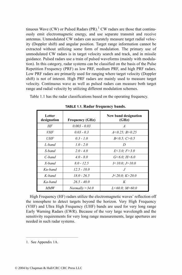
Table 1.1 has the radar classifications based on the operating frequency.
High Frequency (HF) radars utilize the electromagnetic waves reflection off the ionosphere to detect targets beyond the horizon. Very High Frequency (VHF) and Ultra High Frequency (UHF) bands are used for very long range Early Warning Radars (EWR). Because of the very large wavelength and the sensitivity requirements for very long range measurements, large apertures are needed in such radar systems.
1. See Appendix 1A.
TABLE 1.1. Radar frequency bands.
Letter designation Frequency (GHz)
New band designation (GHz)
HF 0.003 - 0.03 A
VHF 0.03 - 0.3 A<0.25; B>0.25
UHF 0.3 - 1.0 B<0.5; C>0.5
L-band 1.0 - 2.0 D
S-band 2.0 - 4.0 E<3.0; F>3.0
C-band 4.0 - 8.0 G<6.0; H>6.0
X-band 8.0 - 12.5 I<10.0; J>10.0
Ku-band 12.5 - 18.0 J
K-band 18.0 - 26.5 J<20.0; K>20.0
Ka-band 26.5 - 40.0 K
MMW Normally >34.0 L<60.0; M>60.0
4 by Chapman & Hall/CRC CRC Press LLC

© 200
Radars in the L-band are primarily ground based and ship based systems that are used in long range military and air traffic control search operations. Most ground and ship based medium range radars operate in the S-band. Most weather detection radar systems are C-band radars. Medium range search and fire control military radars and metric instrumentation radars are also C-band.
The X-band is used for radar systems where the size of the antenna consti-tutes a physical limitation; this includes most military multimode airborne radars. Radar systems that require fine target detection capabilities and yet can-not tolerate the atmospheric attenuation of higher frequency bands may also be X-band. The higher frequency bands (Ku, K, and Ka) suffer severe weather and atmospheric attenuation. Therefore, radars utilizing these frequency bands are limited to short range applications, such as police traffic radar, short range terrain avoidance, and terrain following radar. Milli-Meter Wave (MMW) radars are mainly limited to very short range Radio Frequency (RF) seekers and experimental radar systems.
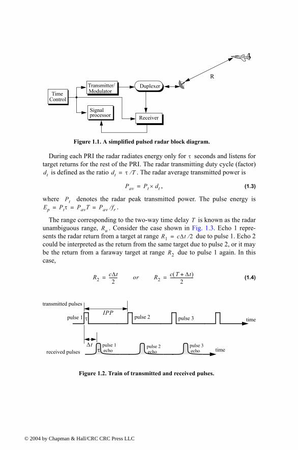
1.2. RangeFigure 1.1 shows a simplified pulsed radar block diagram. The time control
box generates the synchronization timing signals required throughout the sys-tem. A modulated signal is generated and sent to the antenna by the modulator/transmitter block. Switching the antenna between the transmitting and receiv-ing modes is controlled by the duplexer. The duplexer allows one antenna to be used to both transmit and receive. During transmission it directs the radar elec-tromagnetic energy towards the antenna. Alternatively, on reception, it directs the received radar echoes to the receiver. The receiver amplifies the radar returns and prepares them for signal processing. Extraction of target informa-tion is performed by the signal processor block. The targets range, , is com-puted by measuring the time delay, , it takes a pulse to travel the two-way path between the radar and the target. Since electromagnetic waves travel at the speed of light, , then
(1.1)
where is in meters and is in seconds. The factor of is needed to account for the two-way time delay.
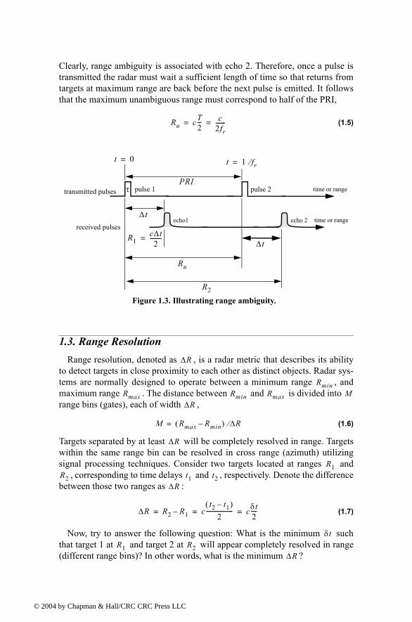
In general, a pulsed radar transmits and receives a train of pulses, as illus-trated by Fig. 1.2. The Inter Pulse Period (IPP) is , and the pulsewidth is . The IPP is often referred to as the Pulse Repetition Interval (PRI). The inverse of the PRI is the PRF, which is denoted by ,
(1.2)
R∆t
c 3 108× m sec⁄=
R c∆t2
--------=
R ∆t 12---
T τ
fr
fr1
PRI---------- 1
T---= =
4 by Chapman & Hall/CRC CRC Press LLC
© 200
During each PRI the radar radiates energy only for seconds and listens for target returns for the rest of the PRI. The radar transmitting duty cycle (factor)
is defined as the ratio . The radar average transmitted power is
, (1.3)
where denotes the radar peak transmitted power. The pulse energy is .
The range corresponding to the two-way time delay is known as the radar unambiguous range, . Consider the case shown in Fig. 1.3. Echo 1 repre-sents the radar return from a target at range due to pulse 1. Echo 2 could be interpreted as the return from the same target due to pulse 2, or it may be the return from a faraway target at range due to pulse 1 again. In this case,
(1.4)
Signalprocessor
TimeControl
Transmitter/Modulator
Signalprocessor Receiver
R
Figure 1.1. A simplified pulsed radar block diagram.
Duplexer
τ
dt dt τ T⁄=
Pav Pt dt×=
PtEp Ptτ PavT Pav fr⁄= = =
TRu
R1 c∆t 2⁄=
R2
R2c∆t2
--------= or R2c T ∆t+( )
2-----------------------=
time
time
transmitted pulses
received pulses
τIPP
pulse 1
∆t
pulse 3pulse 2
τpulse 1 echo
pulse 2 echo
pulse 3 echo
Figure 1.2. Train of transmitted and received pulses.
4 by Chapman & Hall/CRC CRC Press LLC
© 200
Clearly, range ambiguity is associated with echo 2. Therefore, once a pulse is transmitted the radar must wait a sufficient length of time so that returns from targets at maximum range are back before the next pulse is emitted. It follows that the maximum unambiguous range must correspond to half of the PRI,
(1.5)
1.3. Range ResolutionRange resolution, denoted as , is a radar metric that describes its ability
to detect targets in close proximity to each other as distinct objects. Radar sys-tems are normally designed to operate between a minimum range , and maximum range . The distance between and is divided into range bins (gates), each of width ,
(1.6)
Targets separated by at least will be completely resolved in range. Targets within the same range bin can be resolved in cross range (azimuth) utilizing signal processing techniques. Consider two targets located at ranges and
, corresponding to time delays and , respectively. Denote the difference between those two ranges as :
(1.7)
Now, try to answer the following question: What is the minimum such that target 1 at and target 2 at will appear completely resolved in range (different range bins)? In other words, what is the minimum ?
Ru cT2--- c
2fr-------= =
transmitted pulses
received pulses
τPRI
pulse 1
∆t
pulse 2
echo1 echo 2
R1c∆t2
--------=
Ru
R2
∆t
time or range
time or range
t 0= t 1 fr⁄=
Figure 1.3. Illustrating range ambiguity.
∆R
RminRmax Rmin Rmax M
∆R
M Rmax Rmin( ) ∆R⁄=
∆R
R1R2 t1 t2
∆R
∆R R2 R1 ct2 t1( )
2------------------- cδt
2----= = =
δtR1 R2
∆R
4 by Chapman & Hall/CRC CRC Press LLC
© 200
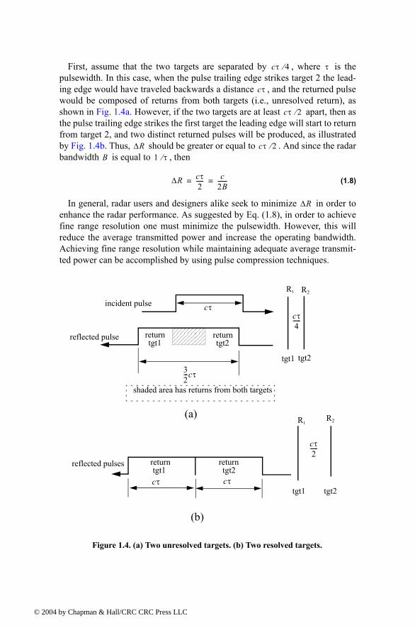
First, assume that the two targets are separated by , where is the pulsewidth. In this case, when the pulse trailing edge strikes target 2 the lead-ing edge would have traveled backwards a distance , and the returned pulse would be composed of returns from both targets (i.e., unresolved return), as shown in Fig. 1.4a. However, if the two targets are at least apart, then as the pulse trailing edge strikes the first target the leading edge will start to return from target 2, and two distinct returned pulses will be produced, as illustrated by Fig. 1.4b. Thus, should be greater or equal to . And since the radar bandwidth is equal to , then
(1.8)
In general, radar users and designers alike seek to minimize in order to enhance the radar performance. As suggested by Eq. (1.8), in order to achieve fine range resolution one must minimize the pulsewidth. However, this will reduce the average transmitted power and increase the operating bandwidth. Achieving fine range resolution while maintaining adequate average transmit-ted power can be accomplished by using pulse compression techniques.
cτ 4⁄ τ
cτ
cτ 2⁄
∆R cτ 2⁄B 1 τ⁄
∆R cτ2----- c
2B-------= =
∆R
incident pulse
reflected pulse
cτ
32---cτ
returntgt1
tgt1 tgt2
cτ4-----
tgt1 tgt2
cτ2-----
(a)
(b)
reflected pulses
cτcτ
return tgt1
return tgt2
R2
R2
R1
R1
return tgt2
shaded area has returns from both targets
Figure 1.4. (a) Two unresolved targets. (b) Two resolved targets.
4 by Chapman & Hall/CRC CRC Press LLC
© 200
1.4. Doppler FrequencyRadars use Doppler frequency to extract target radial velocity (range rate), as
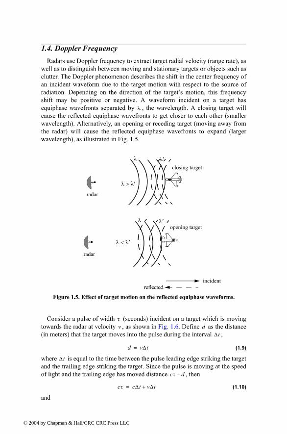
well as to distinguish between moving and stationary targets or objects such as clutter. The Doppler phenomenon describes the shift in the center frequency of an incident waveform due to the target motion with respect to the source of radiation. Depending on the direction of the targets motion, this frequency shift may be positive or negative. A waveform incident on a target has equiphase wavefronts separated by , the wavelength. A closing target will cause the reflected equiphase wavefronts to get closer to each other (smaller wavelength). Alternatively, an opening or receding target (moving away from the radar) will cause the reflected equiphase wavefronts to expand (larger wavelength), as illustrated in Fig. 1.5.
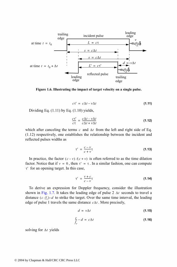
Consider a pulse of width (seconds) incident on a target which is moving towards the radar at velocity , as shown in Fig. 1.6. Define as the distance (in meters) that the target moves into the pulse during the interval ,
(1.9)
where is equal to the time between the pulse leading edge striking the target and the trailing edge striking the target. Since the pulse is moving at the speed of light and the trailing edge has moved distance , then
(1.10)
and
λ
λ λ′>
λ′λ
reflected
λ′
incident
opening target
closing target
λ
λ λ′<
radar
radar
Figure 1.5. Effect of target motion on the reflected equiphase waveforms.
τv d
∆t
d v∆t=
∆t
cτ d
cτ c∆t v∆t+=
4 by Chapman & Hall/CRC CRC Press LLC
© 200
(1.11)
Dividing Eq. (1.11) by Eq. (1.10) yields,
(1.12)
which after canceling the terms and from the left and right side of Eq. (1.12) respectively, one establishes the relationship between the incident and reflected pulses widths as
(1.13)
In practice, the factor is often referred to as the time dilation factor. Notice that if , then . In a similar fashion, one can compute
for an opening target. In this case,
(1.14)
To derive an expression for Doppler frequency, consider the illustration shown in Fig. 1.7. It takes the leading edge of pulse 2 seconds to travel a distance to strike the target. Over the same time interval, the leading edge of pulse 1 travels the same distance . More precisely,
(1.15)
(1.16)
solving for yields
v
s c∆t=
L cτ=
d v∆t=
trailingedge
leadingedgeincident pulse
reflected pulse
s c∆t=
L' cτ'=
leadingedge
trailingedge
at time t t0=
at time t t0 ∆t+=
Figure 1.6. Illustrating the impact of target velocity on a single pulse.
cτ' c∆t v∆t=
cτ'cτ------ c∆t v∆t
c∆t v∆t+-----------------------=
c ∆t
τ′ c vc v+-----------τ=
c v( ) c v+( )⁄v 0= τ′ τ=
τ′
τ′ v c+c v-----------τ=
∆tc fr⁄( ) d
c∆t
d v∆t=
cfr--- d c∆t=
∆t
4 by Chapman & Hall/CRC CRC Press LLC
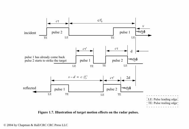
TE: Pulse trailing edgeLE: Pulse leading edge
v
es.
© 2004 by Chapman & Hall/CRC CRC Press LLC© 2004 by Chapman & Hall/CRC CRC Press LLC© 2004 by Chapman & Hall/CRC CRC Press LLC© 2004 by Chapman & Hall/CRC CRC Press LLC© 2004 by Chapman & Hall/CRC CRC Press LLC
pulse 1pulse 2
pulse 1 pulse 2
LETE
TELE
d
c/fr
TE
LETE
incident
reflected
LE
cτ
cτ'
LELE TETE
cτ's d c fr'⁄=
pulse 1 pulse 2
cτ
pulse 1 has already come backpulse 2 starts to strike the target
2d
Figure 1.7. Illustration of target motion effects on the radar puls
© 2004 by Chapman & Hall/CRC CRC Press LLC
© 200
(1.17)
(1.18)
The reflected pulse spacing is now and the new PRF is , where
(1.19)
It follows that the new PRF is related to the original PRF by
(1.20)
However, since the number of cycles does not change, the frequency of the reflected signal will go up by the same factor. Denoting the new frequency by
, it follows
(1.21)
where is the carrier frequency of the incident signal. The Doppler frequency is defined as the difference . More precisely,
(1.22)
but since and , then
(1.23)
Eq. (1.23) indicates that the Doppler shift is proportional to the target velocity, and, thus, one can extract from range rate and vice versa.
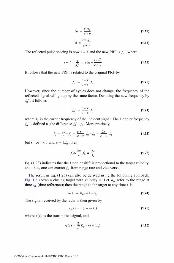
The result in Eq. (1.23) can also be derived using the following approach: Fig. 1.8 shows a closing target with velocity . Let refer to the range at time (time reference); then the range to the target at any time is
(1.24)
The signal received by the radar is then given by
(1.25)
where is the transmitted signal, and
(1.26)
∆tc fr⁄c v+-----------=
dcv fr⁄c v+-------------=
s d fr′
s d cfr′----- c∆t
cv fr⁄c v+-------------= =
fr′c v+c v----------- fr=
f0′
f0′c v+c v----------- f0=
f0fd f0′ f0
fd f0′ f0c v+c v----------- f0 f0
2vc v----------- f0= = =
v c« c λf0=
fd2vc
------ f0≈ 2vλ------=
fd
v R0t0 t
R t( ) R0 v t t0( )=
xr t( ) x t ψ t( )( )=
x t( )
ψ t( ) 2c--- R0 vt vt0+( )=
4 by Chapman & Hall/CRC CRC Press LLC
© 200
Substituting Eq. (1.26) into Eq. (1.25) and collecting terms yield
(1.27)
where the constant phase is
(1.28)
Define the compression or scaling factor by
(1.29)
Note that for a receding target the scaling factor is . Utilizing Eq. (1.29) we can rewrite Eq. (1.27) as
(1.30)
Eq. (1.30) is a time-compressed version of the return signal from a stationary target ( ). Hence, based on the scaling property of the Fourier transform, the spectrum of the received signal will be expanded in frequency to a factor of
.
Consider the special case when
(1.31)
where is the radar center frequency in radians per second. The received sig-nal is then given by
(1.32)
The Fourier transform of Eq. (1.32) is
(1.33)
v
R0
Figure 1.8. Closing target with velocity v.
xr t( ) x 1 2vc
------+ t ψ0 =
ψ0
ψ02R0
c--------- 2v
c------+ t0=
γ
γ 1 2vc
------+=
γ 1 2v c⁄( )=
xr t( ) x γt ψ0( )=
v 0=
γ
x t( ) y t( ) ω0tcos=
ω0xr t( )
xr t( ) y γt ψ0( ) γω0t ψ0( )cos=
Xr ω( ) 12γ----- Y ω
γ---- ω0 Y ω
γ---- ω0+ +
=
4 by Chapman & Hall/CRC CRC Press LLC
© 2
where for simplicity the effects of the constant phase have been ignored in Eq. (1.33). Therefore, the bandpass spectrum of the received signal is now cen-tered at instead of . The difference between the two values corresponds to the amount of Doppler shift incurred due to the target motion,
(1.34)
is the Doppler frequency in radians per second. Substituting the value of in Eq. (1.34) and using yield
(1.35)
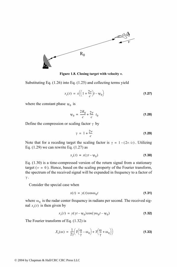
which is the same as Eq. (1.23). It can be shown that for a receding target the Doppler shift is . This is illustrated in Fig. 1.9.
In both Eq. (1.35) and Eq. (1.23) the target radial velocity with respect to the radar is equal to , but this is not always the case. In fact, the amount of Dop-pler frequency depends on the target velocity component in the direction of the radar (radial velocity). Fig. 1.10 shows three targets all having velocity : tar-get 1 has zero Doppler shift; target 2 has maximum Doppler frequency as defined in Eq. (1.35). The amount of Doppler frequency of target 3 is
, where is the radial velocity; and is the total angle between the radar line of sight and the target.
Thus, a more general expression for that accounts for the total angle between the radar and the target is
(1.36)
and for an opening target
(1.37)
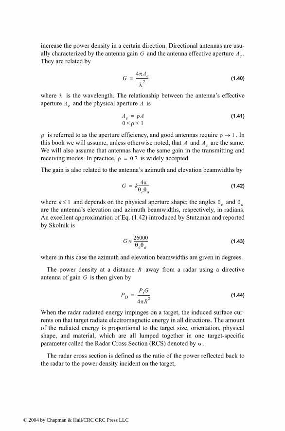
where . The angles and are, respectively, the eleva-tion and azimuth angles; see Fig. 1.11.
ψ0
γω0 ω0
ωd ω0 γω0=
ωd γ2πf ω=
fd2vc
------ f02vλ------= =
fd 2v λ⁄=
f0
fd
f0
fd
frequency frequency
ampl
itude
ampl
itude
closing target receding target
Figure 1.9. Spectra of received signal showing Doppler shift.
v
v
fd 2v θcos λ⁄= v θcos θ
fd
fd2vλ------ θcos=
fd2 vλ
--------- θcos=
θcos θecos θacos= θe θa
004 by Chapman & Hall/CRC CRC Press LLC
© 200
1.5. The Radar EquationConsider a radar with an omni directional antenna (one that radiates energy
equally in all directions). Since these kinds of antennas have a spherical radia-tion pattern, we can define the peak power density (power per unit area) at any point in space as
(1.38)
The power density at range away from the radar (assuming a lossless propa-gation medium) is
(1.39)
where is the peak transmitted power and is the surface area of a sphere of radius . Radar systems utilize directional antennas in order to
θv v
v
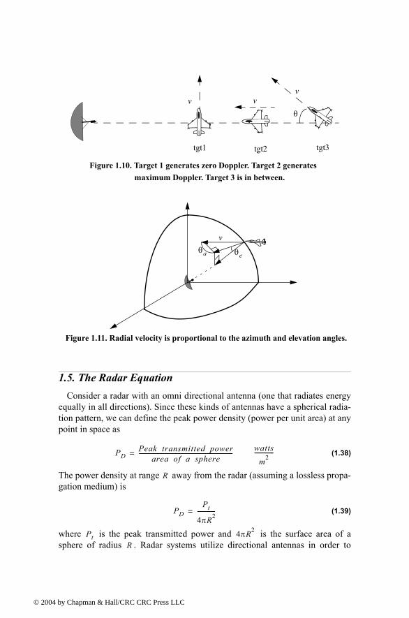
Figure 1.10. Target 1 generates zero Doppler. Target 2 generates maximum Doppler. Target 3 is in between.
tgt1 tgt2 tgt3
vθa θe
Figure 1.11. Radial velocity is proportional to the azimuth and elevation angles.
PDPeak transmitted power
area of a sphere-------------------------------------------------------------------=
wattsm2
--------------
R
PDPt
4πR2-------------=
Pt 4πR2
R
4 by Chapman & Hall/CRC CRC Press LLC
© 200
increase the power density in a certain direction. Directional antennas are usu-ally characterized by the antenna gain and the antenna effective aperture . They are related by
(1.40)
where is the wavelength. The relationship between the antennas effective aperture and the physical aperture is
(1.41)
is referred to as the aperture efficiency, and good antennas require . In this book we will assume, unless otherwise noted, that and are the same. We will also assume that antennas have the same gain in the transmitting and receiving modes. In practice, is widely accepted.
The gain is also related to the antennas azimuth and elevation beamwidths by
(1.42)
where and depends on the physical aperture shape; the angles and are the antennas elevation and azimuth beamwidths, respectively, in radians. An excellent approximation of Eq. (1.42) introduced by Stutzman and reported by Skolnik is
(1.43)
where in this case the azimuth and elevation beamwidths are given in degrees.
The power density at a distance away from a radar using a directive antenna of gain is then given by
(1.44)
When the radar radiated energy impinges on a target, the induced surface cur-rents on that target radiate electromagnetic energy in all directions. The amount of the radiated energy is proportional to the target size, orientation, physical shape, and material, which are all lumped together in one target-specific parameter called the Radar Cross Section (RCS) denoted by .
The radar cross section is defined as the ratio of the power reflected back to the radar to the power density incident on the target,
G Ae
G4πAe
λ2------------=
λAe A
Ae ρA0 ρ 1≤ ≤
=
ρ ρ 1→A Ae
ρ 0.7=
G k 4πθeθa-----------=
k 1≤ θe θa
G 26000θeθa
---------------≈
RG
PDPtG
4πR2-------------=
σ
4 by Chapman & Hall/CRC CRC Press LLC
© 200
(1.45)
where is the power reflected from the target. Thus, the total power deliv-ered to the radar signal processor by the antenna is
(1.46)
Substituting the value of from Eq. (1.40) into Eq. (1.46) yields
(1.47)
Let denote the minimum detectable signal power. It follows that the maximum radar range is
(1.48)
Eq. (1.48) suggests that in order to double the radar maximum range one must increase the peak transmitted power sixteen times; or equivalently, one must increase the effective aperture four times.
In practical situations the returned signals received by the radar will be cor-rupted with noise, which introduces unwanted voltages at all radar frequencies. Noise is random in nature and can be described by its Power Spectral Density (PSD) function. The noise power is a function of the radar operating band-width, . More precisely
(1.49)
The input noise power to a lossless antenna is
(1.50)
where is Boltzmans constant, and is the effective noise temperature in degrees Kelvin. It is always desirable that the minimum detectable signal ( ) be greater than the noise power. The fidelity of a radar receiver is normally described by a figure of merit called the noise figure (see Appendix 1B for details). The noise figure is defined as
(1.51)
and are, respectively, the Signal to Noise Ratios (SNR) at the input and output of the receiver. is the input signal power; is the input
σPrPD------- m2
=
Pr
PDrPtGσ
4πR2( )2
-------------------- Ae=
Ae
PDrPtG
2λ2σ
4π( )3R4----------------------=
SminRmax
RmaxPtG
2λ2σ
4π( )3Smin
-------------------------
1 4⁄
=
Pt
NB
N Noise PSD B×=
Ni kTeB=
k 1.38 10 23× joule degree⁄ Kelvin= Te
Smin
F
FSNR( )iSNR( )o
------------------Si Ni⁄So No⁄----------------= =
SNR( )i SNR( )oSi Ni
4 by Chapman & Hall/CRC CRC Press LLC
© 200
noise power. and are, respectively, the output signal and noise power. Substituting Eq. (1.50) into Eq. (1.51) and rearranging terms yields
(1.52)
Thus, the minimum detectable signal power can be written as
(1.53)
The radar detection threshold is set equal to the minimum output SNR, . Substituting Eq. (1.53) in Eq. (1.48) gives
(1.54)
or equivalently,
(1.55)
In general, radar losses denoted as reduce the overall SNR, and hence
(1.56)
Although it may take on many different forms, Eq. (1.56) is what is widely known as the Radar Equation. It is a common practice to perform calculations associated with the radar equation using decibel (dB) arithmetic. A review is presented in Appendix A.
MATLAB Function radar_eq.m
The function radar_eq.m implements Eq. (1.56); it is given in Listing 1.1 in Section 1.10. The syntax is as follows:
[snr] = radar_eq (pt, freq, g, sigma, te, b, nf, loss, range)
where
Symbol Description Units Status
pt peak power Watts input
freq radar center frequency Hz input
g antenna gain dB input
sigma target cross section m2 input
te effective noise temperature Kelvin input
So No
Si kTeBF SNR( )o=
Smin kTeBF SNR( )omin=
SNR( )omin
RmaxPtG
2λ2σ
4π( )3kTeBF SNR( )omin
------------------------------------------------------- 1 4⁄
=
SNR( )omin
PtG2λ2σ
4π( )3kTeBFRmax4
-------------------------------------------=
L
SNR( )oPtG
2λ2σ
4π( )3kTeBFLR4-----------------------------------------=
4 by Chapman & Hall/CRC CRC Press LLC
© 200
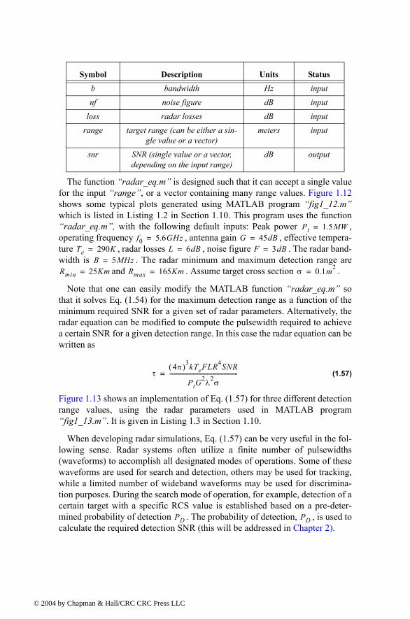
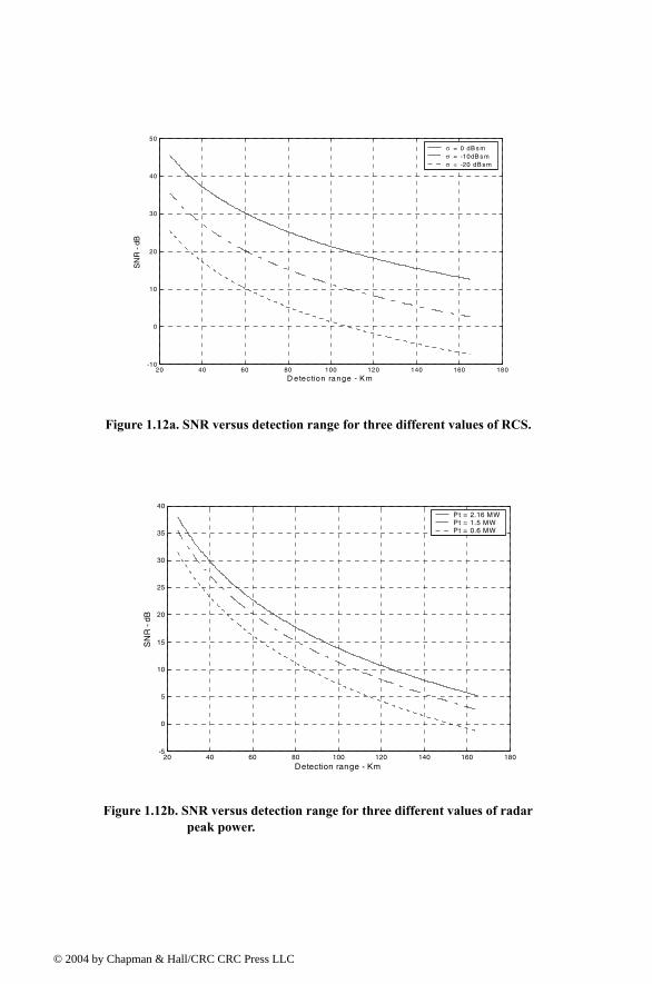
The function radar_eq.m is designed such that it can accept a single value for the input range, or a vector containing many range values. Figure 1.12 shows some typical plots generated using MATLAB program fig1_12.mwhich is listed in Listing 1.2 in Section 1.10. This program uses the function radar_eq.m, with the following default inputs: Peak power , operating frequency , antenna gain , effective tempera-ture , radar losses , noise figure . The radar band-width is . The radar minimum and maximum detection range are
and . Assume target cross section .
Note that one can easily modify the MATLAB function radar_eq.m so that it solves Eq. (1.54) for the maximum detection range as a function of the minimum required SNR for a given set of radar parameters. Alternatively, the radar equation can be modified to compute the pulsewidth required to achieve a certain SNR for a given detection range. In this case the radar equation can be written as
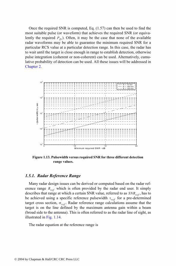
(1.57)
Figure 1.13 shows an implementation of Eq. (1.57) for three different detection range values, using the radar parameters used in MATLAB program fig1_13.m. It is given in Listing 1.3 in Section 1.10.
When developing radar simulations, Eq. (1.57) can be very useful in the fol-lowing sense. Radar systems often utilize a finite number of pulsewidths (waveforms) to accomplish all designated modes of operations. Some of these waveforms are used for search and detection, others may be used for tracking, while a limited number of wideband waveforms may be used for discrimina-tion purposes. During the search mode of operation, for example, detection of a certain target with a specific RCS value is established based on a pre-deter-mined probability of detection . The probability of detection, , is used to calculate the required detection SNR (this will be addressed in Chapter 2).
b bandwidth Hz input
nf noise figure dB input
loss radar losses dB input
range target range (can be either a sin-gle value or a vector)
meters input
snr SNR (single value or a vector, depending on the input range)
dB output
Symbol Description Units Status
Pt 1.5MW=f0 5.6GHz= G 45dB=
Te 290K= L 6dB= F 3dB=B 5MHz=
Rmin 25Km= Rmax 165Km= σ 0.1m2=
τ4π( )3kTeFLR4SNR
PtG2λ2σ
-------------------------------------------------=
PD PD
4 by Chapman & Hall/CRC CRC Press LLC
© 200
Figure 1.12a. SNR versus detection range for three different values of RCS.
20 40 60 80 100 120 140 160 180-10
0
10
20
30
40
50
D etection range - K m
SN
R -
dB
σ = 0 dB s mσ = -10dB s mσ = -20 dB s m
Figure 1.12b. SNR versus detection range for three different values of radar peak power.
20 40 60 80 100 120 140 160 180-5
0
5
10
15
20
25
30
35
40
Detection range - Km
SN
R -
dB
P t = 2.16 MWPt = 1.5 MWPt = 0.6 MW
4 by Chapman & Hall/CRC CRC Press LLC
© 200
Once the required SNR is computed, Eq. (1.57) can then be used to find the most suitable pulse (or waveform) that achieves the required SNR (or equiva-lently the required ). Often, it may be the case that none of the available radar waveforms may be able to guarantee the minimum required SNR for a particular RCS value at a particular detection range. In this case, the radar has to wait until the target is close enough in range to establish detection, otherwise pulse integration (coherent or non-coherent) can be used. Alternatively, cumu-lative probability of detection can be used. All these issues will be addressed in Chapter 2.
1.5.1. Radar Reference Range
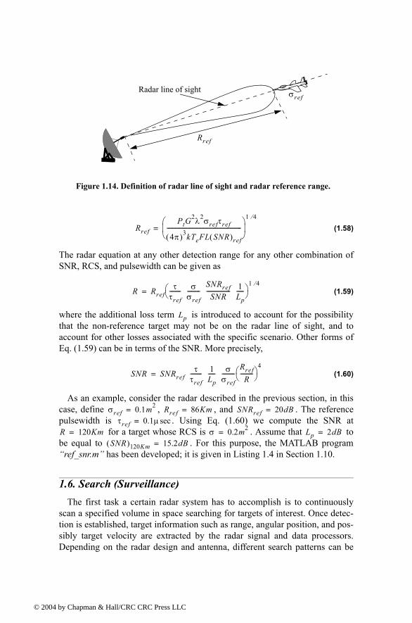
Many radar design issues can be derived or computed based on the radar ref-erence range which is often provided by the radar end user. It simply describes that range at which a certain SNR value, referred to as , has to be achieved using a specific reference pulsewidth for a pre-determined target cross section, . Radar reference range calculations assume that the target is on the line defined by the maximum antenna gain within a beam (broad side to the antenna). This is often referred to as the radar line of sight, as illustrated in Fig. 1.14.
The radar equation at the reference range is
PD
Figure 1.13. Pulsewidth versus required SNR for three different detection range values.
5 10 15 2010
-1
100
101
102
103
Minimum required SN R - dB
τ (p
ulse
wid
th) i
n µ
sec
R = 75 K mR = 100 K mR = 150 K m
RrefSNRref
τrefσref
4 by Chapman & Hall/CRC CRC Press LLC
© 200
(1.58)
The radar equation at any other detection range for any other combination of SNR, RCS, and pulsewidth can be given as
(1.59)
where the additional loss term is introduced to account for the possibility that the non-reference target may not be on the radar line of sight, and to account for other losses associated with the specific scenario. Other forms of Eq. (1.59) can be in terms of the SNR. More precisely,
(1.60)
As an example, consider the radar described in the previous section, in this case, define , , and . The reference pulsewidth is . Using Eq. (1.60) we compute the SNR at
for a target whose RCS is . Assume that to be equal to . For this purpose, the MATLAB program ref_snr.m has been developed; it is given in Listing 1.4 in Section 1.10.
1.6. Search (Surveillance)The first task a certain radar system has to accomplish is to continuously
scan a specified volume in space searching for targets of interest. Once detec-tion is established, target information such as range, angular position, and pos-sibly target velocity are extracted by the radar signal and data processors. Depending on the radar design and antenna, different search patterns can be
Rref
σrefRadar line of sight
Figure 1.14. Definition of radar line of sight and radar reference range.
RrefPtG
2λ2σrefτref
4π( )3kTeFL SNR( )ref
-----------------------------------------------------
1 4⁄
=
R Rrefττref-------- σ
σref---------
SNRrefSNR
----------------- 1Lp-----
1 4⁄
=
Lp
SNR SNRrefττref-------- 1
Lp----- σ
σref---------
RrefR
---------
4=
σref 0.1m2= Rref 86Km= SNRref 20dB=
τref 0.1µ sec=R 120Km= σ 0.2m2
= Lp 2dB=SNR( )120Km 15.2dB=
4 by Chapman & Hall/CRC CRC Press LLC
© 200
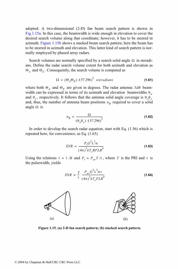
adopted. A two-dimensional (2-D) fan beam search pattern is shown in Fig.1.15a. In this case, the beamwidth is wide enough in elevation to cover the desired search volume along that coordinate; however, it has to be steered in azimuth. Figure 1.15b shows a stacked beam search pattern; here the beam has to be steered in azimuth and elevation. This latter kind of search pattern is nor-mally employed by phased array radars.
Search volumes are normally specified by a search solid angle in steradi-ans. Define the radar search volume extent for both azimuth and elevation as
and . Consequently, the search volume is computed as
(1.61)
where both and are given in degrees. The radar antenna beam-width can be expressed in terms of its azimuth and elevation beamwidths and , respectively. It follows that the antenna solid angle coverage is and, thus, the number of antenna beam positions required to cover a solid angle is
(1.62)
In order to develop the search radar equation, start with Eq. (1.56) which is repeated here, for convenience, as Eq. (1.63)
(1.63)
Using the relations and , where is the PRI and is the pulsewidth, yields
(1.64)
Ω
ΘA ΘE
Ω ΘAΘE( ) 57.296( )2⁄ steradians=
ΘA ΘE 3dBθa
θe θaθenB
Ω
nBΩ
θaθe( ) 57.296( )2⁄--------------------------------------------=
SNRPtG
2λ2σ
4π( )3kTeBFLR4-----------------------------------------=
τ 1 B⁄= Pt PavT τ⁄= T τ
SNR Tτ---
PavG2λ2στ
4π( )3kTeFLR4-------------------------------------=
(a) (b)
Figure 1.15. (a) 2-D fan search pattern; (b) stacked search pattern.
4 by Chapman & Hall/CRC CRC Press LLC
© 200
Define the time it takes the radar to scan a volume defined by the solid angle as the scan time . The time on target can then be expressed in terms of as
(1.65)
Assume that during a single scan only one pulse per beam per PRI illuminates the target. It follows that and, thus, Eq. (1.64) can be written as
(1.66)
Substituting Eqs. (1.40) and (1.42) into Eq. (1.66) and collecting terms yield the search radar equation (based on a single pulse per beam per PRI) as
(1.67)
The quantity in Eq. (1.67) is known as the power aperture product. In practice, the power aperture product is widely used to categorize the radars ability to fulfill its search mission. Normally, a power aperture product is com-puted to meet a predetermined SNR and radar cross section for a given search volume defined by .
As a special case, assume a radar using a circular aperture (antenna) with diameter . The 3-dB antenna beamwidth is
(1.68)
and when aperture tapering is used, . Substituting Eq. (1.68) into Eq. (1.62) yields
(1.69)
For this case, the scan time is related to the time-on-target by
(1.70)
Substitute Eq. (1.70) into Eq. (1.64) to get
(1.71)
Ω TscTsc
TiTscnB-------
TscΩ
-------θaθe= =
Ti T=
SNRPavG2λ2σ
4π( )3kTeFLR4-------------------------------------
TscΩ
-------θaθe=
SNRPavAeσ
4πkTeFLR4-----------------------------
TscΩ
-------=
PavA
Ω
D θ3dB
θ3dBλD----≈
θ3dB 1.25λ D⁄≈
nBD2
λ2------ Ω=
Tsc
TiTscnB-------
Tscλ2
D2Ω--------------= =
SNRPavG2λ2σ
4π( )3R4kTeFL-------------------------------------
Tscλ2
D2Ω--------------=
4 by Chapman & Hall/CRC CRC Press LLC
© 200
and by using Eq. (1.40) in Eq. (1.71) we can define the search radar equation for a circular aperture as
(1.72)
where the relation (aperture area) is used.
MATLAB Function power_aperture.m
The function power_aperture.m implements the search radar equation given in Eq. (1.67); it is given in Listing 1.5 in Section 1.10. The syntax is as follows:
PAP = power_aperture (snr, tsc, sigma, range, te, nf, loss, az_angle, el_angle)
where
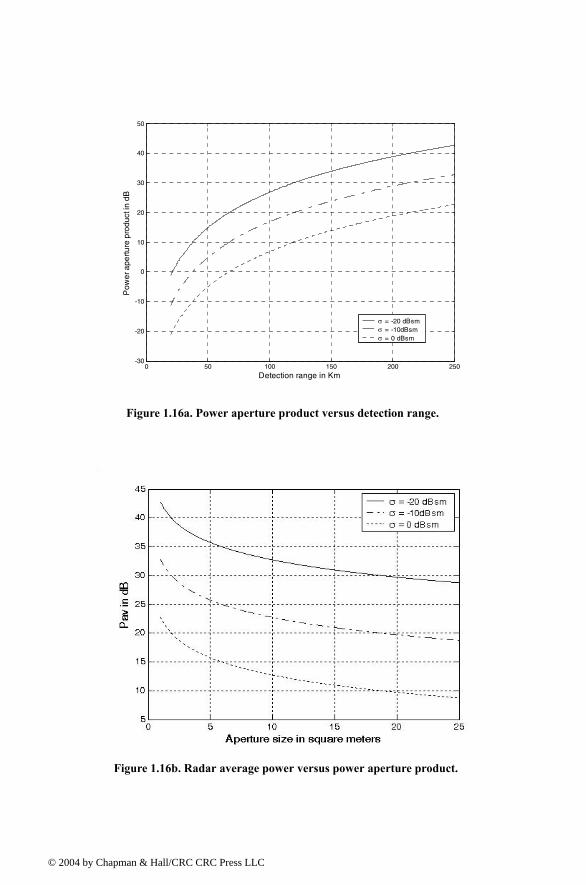
Plots of the power aperture product versus range and plots of the average power versus aperture area for three RCS choices are shown in Figure 1.16. MATLAB program fig1_16.m was used to produce these figures. It is given in Listing 1.6 in Section 1.10. In this case, the following radar parameters were used
Symbol Description Units Status
snr sensitivity snr dB input
tsc scan time seconds input
sigma target cross section m2 input
range target range (can be either sin-gle value or a vector)
meters input
te effective temperature Kelvin input
nf noise figure dB input
loss radar losses dB input
az_angle search volume azimuth extent degrees input
el_angle search volume elevation extent degrees input
PAP power aperture product dB output
SNRPavAσ
16R4kTeLF-----------------------------
Tsc
Ω-------=
A πD2 4⁄=
σ Tsc θe θa= R Te nf loss× snr
0.1 m2 2.5sec 2° 250Km 900K 13dB 15dB
4 by Chapman & Hall/CRC CRC Press LLC
© 200
Figure 1.16a. Power aperture product versus detection range.
0 50 100 150 200 250-30
-20
-10
0
10
20
30
40
50
Detection range in Km
Pow
er a
pertu
re p
rodu
ct in
dB
σ = -20 dBsmσ = -10dBsmσ = 0 dBsm
Figure 1.16b. Radar average power versus power aperture product.
4 by Chapman & Hall/CRC CRC Press LLC
© 200
Example:
Compute the power aperture product corresponding to the radar that has the following parameters: Scan time , Noise figure , losses
, search volume , range of interest is , and the required SNR is . Assume that and
.
Solution:
Note that corresponds to a search sector that is three fourths of a hemisphere. Thus, using Eq. (1.61) we conclude that
and . Using the MATLAB function power_aperture.m with the fol-lowing syntax:
PAP = power_aperture(20, 2, 3.162, 75e3, 290, 8, 6, 180, 135)
we compute the power aperture product as 36.7 dB.
1.6.1. Mini Design Case Study 1.1
Problem Statement:Design a ground based radar that is capable of detecting aircraft and mis-
siles at 10 Km and 2 Km altitudes, respectively. The maximum detection range for either target type is 60 Km. Assume that an aircraft average RCS is 6 dBsm, and that a missile average RCS is -10 dBsm. The radar azimuth and elevation search extents are respectively and . The required scan rate is 2 seconds and the range resolution is 150 meters. Assume a noise figure F = 8 dB, and total receiver noise L = 10 dB. Use a fan beam with azimuth beamwidth less than 3 degrees. The SNR is 15 dB.
A Design:The range resolution requirement is ; thus by using Eq. (1.8) we
calculate the required pulsewidth , or equivalently require the bandwidth . The statement of the problem lends itself to radar siz-ing in terms of power aperture product. For this purpose, one must first com-pute the maximum search volume at the detection range that satisfies the design requirements. The radar search volume is
(1.73)
At this point, the designer is ready to use the radar search equation (Eq. (1.67)) to compute the power aperture product. For this purpose, one can mod-
Tsc 2sec= F 8dB=
L 6dB= Ω 7.4 steradians= R 75Km=
20dB Te 290Kelvin=
σ 3.162m2=
Ω 7.4 steradians=
θa 180°=
θe 135°=
ΘA 360°= ΘE 10°=
∆R 150m=τ 1µ sec=
B 1MHz=
ΩΘAΘE
57.296( )2----------------------- 360 10×
57.296( )2----------------------- 1.097 steradians= = =
4 by Chapman & Hall/CRC CRC Press LLC
© 200
ify the MATLAB function power_aperture.m to compute and plot the power aperture product for both target types. To this end, the MATLAB program casestudy1_1.m, which is given in Listing 1.7 in Section 1.10, was devel-oped. Use the parameters in Table 1.2 as inputs for this program. Note that the selection of is arbitrary.
TABLE 1.2: Input parameters to MATLAB program casestudy1_1.m.
Figure 1.17 shows a plot of the output produced by this program. The same program also calculates the corresponding power aperture product for both the missile and aircraft cases, which can also be read from the plot,
(1.74)
Choosing the more stressing case for the design baseline (i.e., select the power-aperture-product resulting from the missile analysis) yields
(1.75)
Choose to calculate the average power as
(1.76)
and assuming an aperture efficiency of yields the physical aperture area. More precisely,
(1.77)
Symbol Description Units Value
snr sensitivity snr dB 15
tsc scan time seconds 2
sigma_tgtm missile radar cross section dBsm -10
sigma_tgta aircraft radar cross section dBsm 6
rangem missile detection range Km 60
rangea aircraft detection range Km 60
te effective temperature Kelvin 290
nf noise figure dB 8
loss radar losses dB 10
az_angle search volume azimuth extent degrees 360
el_angle search volume elevation extent degrees 10
Te 290Kelvin=
PAPmissile 38.53dB=
PAPaircraft 22.53dB=
Pav Ae× 103.853 7128.53 Ae⇒ 7128.53Pav
-------------------= = =
Ae 1.75m2=
Pav7128.53
1.75------------------- 4.073KW= =
ρ 0.8=
AAeρ----- 1.75
0.8---------- 2.1875m2
= = =
4 by Chapman & Hall/CRC CRC Press LLC
© 200
Use as the radar operating frequency. Then by using we calculate using Eq. (1.40) . Now one must deter-
mine the antenna azimuth beamwidth. Recall that the antenna gain is also related to the antenna 3-dB beamwidth by the relation
(1.78)
where are the antenna 3-dB azimuth and elevation beamwidths, respectively. Assume a fan beam with . It follows that
(1.79)
1.7. Pulse Integration When a target is located within the radar beam during a single scan it may
reflect several pulses. By adding the returns from all pulses returned by a given target during a single scan, the radar sensitivity (SNR) can be increased. The number of returned pulses depends on the antenna scan rate and the radar PRF. More precisely, the number of pulses returned from a given target is given by
(1.80)
Figure 1.17. Power aperture product versus detection range for radar in mini design case study 1.1.
f0 2.0GHz=Ae 1.75m2
= G 29.9dB=
G 26000θeθa
---------------=
θa θe,( )θe ΘE= 15°=
θa26000θeG
--------------- 2600010 977.38×---------------------------- 2.66°= = = θa⇒ 46.43mrad=
nPθaTscfr
2π-----------------=
4 by Chapman & Hall/CRC CRC Press LLC
© 200
where is the azimuth antenna beamwidth, is the scan time, and is the radar PRF. The number of reflected pulses may also be expressed as
(1.81)
where is the antenna scan rate in degrees per second. Note that when using Eq. (1.80), is expressed in radians, while when using Eq. (1.81) it is expressed in degrees. As an example, consider a radar with an azimuth antenna beamwidth , antenna scan rate (antenna scan time,
), and a PRF . Using either Eq.s (1.80) or (1.81) yields pulses.
The process of adding radar returns from many pulses is called radar pulse integration. Pulse integration can be performed on the quadrature components prior to the envelope detector. This is called coherent integration or pre-detec-tion integration. Coherent integration preserves the phase relationship between the received pulses. Thus a build up in the signal amplitude is achieved. Alter-natively, pulse integration performed after the envelope detector (where the phase relation is destroyed) is called non-coherent or post-detection integra-tion.
Radar designers should exercise caution when utilizing pulse integration for the following reasons. First, during a scan a given target will not always be located at the center of the radar beam (i.e., have maximum gain). In fact, dur-ing a scan a given target will first enter the antenna beam at the 3-dB point, reach maximum gain, and finally leave the beam at the 3-dB point again. Thus, the returns do not have the same amplitude even though the target RCS may be constant and all other factors which may introduce signal loss remain the same. This is illustrated in Fig. 1.18, and is normally referred to as antenna beam-shape loss.
θa Tsc fr
nPθafr
θ· scan------------=
θ· scanθa
θa 3°= θ· scan 45° sec⁄=Tsc 8 ondssec= fr 300Hz=
nP 20=
time
ampl
itude
antenna 3-dB beamwidth
Figure 1.18. Pulse returns from a point target using a rotating (scanning) antenna
4 by Chapman & Hall/CRC CRC Press LLC
© 200
Other factors that may introduce further variation to the amplitude of the returned pulses include target RCS and propagation path fluctuations. Addi-tionally, when the radar employs a very fast scan rate, an additional loss term is introduced due to the motion of the beam between transmission and reception. This is referred to as scan loss. A distinction should be made between scan loss due to a rotating antenna (which is described here) and the term scan loss that is normally associated with phased array antennas (which takes on a different meaning in that context). These topics will be discussed in more detail in other chapters.
Finally, since coherent integration utilizes the phase information from all integrated pulses, it is critical that any phase variation between all integrated pulses be known with a great level of confidence. Consequently, target dynam-ics (such as target range, range rate, tumble rate, RCS fluctuation, etc.) must be estimated or computed accurately so that coherent integration can be meaning-ful. In fact, if a radar coherently integrates pulses from targets without proper knowledge of the target dynamics it suffers a loss in SNR rather than the expected SNR build up. Knowledge of target dynamics is not as critical when employing non-coherent integration; nonetheless, target range rate must be estimated so that only the returns from a given target within a specific range bin are integrated. In other words, one must avoid range walk (i.e., avoid hav-ing a target cross between adjacent range bins during a single scan).
A comprehensive analysis of pulse integration should take into account issues such as the probability of detection , probability of false alarm , the target statistical fluctuation model, and the noise or interference statistical models. These topics will be discussed in Chapter 2. However, in this section an overview of pulse integration is introduced in the context of radar measure-ments as it applies to the radar equation. The basic conclusions presented in this chapter concerning pulse integration will still be valid, in the general sense, when a more comprehensive analysis of pulse integration is presented; however, the exact implementation, the mathematical formulation, and /or the numerical values used will vary.
1.7.1. Coherent IntegrationIn coherent integration, when a perfect integrator is used (100% efficiency),
to integrate pulses the SNR is improved by the same factor. Otherwise, integration loss occurs, which is always the case for non-coherent integration. Coherent integration loss occurs when the integration process is not optimum. This could be due to target fluctuation, instability in the radar local oscillator, or propagation path changes.
Denote the single pulse SNR required to produce a given probability of detection as . The SNR resulting from coherently integrating pulses is then given by
PD Pfa
nP
SNR( )1 nP
4 by Chapman & Hall/CRC CRC Press LLC
© 200
(1.82)
Coherent integration cannot be applied over a large number of pulses, partic-ularly if the target RCS is varying rapidly. If the target radial velocity is known and no acceleration is assumed, the maximum coherent integration time is lim-ited to
(1.83)
where is the radar wavelength and is the target radial acceleration. Coher-ent integration time can be extended if the target radial acceleration can be compensated for by the radar.
1.7.2. Non-Coherent Integration
Non-coherent integration is often implemented after the envelope detector, also known as the quadratic detector. Non-coherent integration is less efficient than coherent integration. Actually, the non-coherent integration gain is always smaller than the number of non-coherently integrated pulses. This loss in inte-gration is referred to as post detection or square law detector loss. Marcum and Swerling showed that this loss is somewhere between and . DiFranco and Rubin presented an approximation of this loss as
(1.84)
Note that as becomes very large, the integration loss approaches .
The subject of integration loss is treated in great levels of detail in the litera-ture. Different authors use different approximations for the integration loss associated with non-coherent integration. However, all these different approxi-mations yield very comparable results. Therefore, in the opinion of these authors the use of one formula or another to approximate integration loss becomes somewhat subjective. In this book, the integration loss approximation reported by Barton and used by Curry will be adopted. In this case, the non-coherent integration loss which can be used in the radar equation is
(1.85)
It follows that the SNR when pulses are integrated non-coherently is
(1.86)
1.7.3. Detection Range with Pulse Integration
The process of determining the radar sensitivity or equivalently the maxi-mum detection range when pulse integration is used is as follows: First, decide
SNR( )CI nP SNR( )1=
tCI λ 2ar⁄=
λ ar
nP nP
LNCI 10 np( )log 5.5 dB=
nP nP
LNCI1 SNR( )1+
SNR( )1----------------------------=
nP
SNR( )NCInP SNR( )1
LNCI------------------------- nP SNR( )1
SNR( )11 SNR( )1+----------------------------×= =
4 by Chapman & Hall/CRC CRC Press LLC
© 200
whether to use coherent or non-coherent integration. Keep in mind the issues discussed in the beginning of this section when deciding whether to use coher-ent or non-coherent integration.
Second, determine the minimum required or required for adequate detection and track. Typically, for ground based surveillance radars that can be on the order of 13 to 15 dB. The third step is to determine how many pulses should be integrated. The choice of is affected by the radar scan rate, the radar PRF, the azimuth antenna beamwidth, and of course by the target dynamics (remember that range walk should be avoided or compensated for, so that proper integration is feasible). Once and the required SNR are known one can compute the single pulse SNR (i.e., the reduction in SNR). For this purpose use Eq. (1.82) in the case of coherent integration. In the non-coherent integration case, Curry presents an attractive formula for this calcula-tion, as follows
(1.87)
Finally, use from Eq. (1.87) in the radar equation to calculate the radar detection range. Observe that due to the integration reduction in SNR the radar detection range is now larger than that for the single pulse when the same SNR value is used. This is illustrated using the following mini design case study.
1.7.4. Mini Design Case Study 1.2
Problem Statement:
A MMW radar has the following specifications: Center frequency
, pulsewidth , peak power , azimuth cov-
erage , Pulse repetition frequency , noise figure ; antenna diameter ; antenna gain ; radar cross
section of target is ; system losses ; radar scan time . Calculate: The wavelength ; range resolution ; bandwidth
; antenna half power beamwidth; antenna scan rate; time on target. Com-pute the range that corresponds to 10 dB SNR. Plot the SNR as a function of range. Finally, compute the number of pulses on the target that can be used for integration and the corresponding new detection range when pulse integration is used, assuming that the SNR stays unchanged (i.e., the same as in the case of a single pulse). Assume .
SNR( )CI SNR( )NCI
nP
nP
SNR( )1SNR( )NCI
2nP------------------------
SNR( )NCI2
4nP2
------------------------SNR( )NCI
nP------------------------++=
SNR( )1
f 94GHz= τ 50 10 9× sec= Pt 4W=
∆α 120°±= PRF 10KHz=
F 7dB= D 12in= G 47dB=
σ 20m2= L 10dB=
Tsc 3sec= λ ∆R
B
Te 290 Kelvin=
4 by Chapman & Hall/CRC CRC Press LLC
© 200
A Design:
The wavelength is
The range resolution is
Radar operating bandwidth is
The antenna 3-dB beamwidth is
Time on target is
It follows that the number of pulses available for integration is calculated using Eq. (1.81),
Coherent Integration case:Using the radar equation given in Eq. (1.58) yields . The
SNR improvement due to coherently integrating 94 pulses is 19.73dB. How-ever, since it is requested that the SNR remains at 10dB, we can calculate the new detection range using Eq. (1.59) as
Using the MATLAB Function radar_eq.m with the following syntax
[snr] = radar_eq (4, 94e9, 47, 20, 290, 20e6, 7, 10, 6.99e3)
yields SNR = -9.68 dB. This means that using 94 pulses integrated coherently at 6.99 Km where each pulse has a SNR of -9.68 dB provides the same detec-tion criteria as using a single pulse with SNR = 10dB at 2.245Km. This is illus-trated in Fig. 1.19, using the MATLAB program fig1_19.m, which is given in Listing 1.8 in Section 1.10. Figure 1.19 shows the improvement of the detection range if the SNR is kept constant before and after integration.
λ
λ cf-- 3 108×
94 109×-------------------- 0.00319m= = =
∆R
∆R cτ2----- 3 108×( ) 50 10 9×( )
2--------------------------------------------------- 7.5m= = =
B
B 1τ--- 1
50 10 9×----------------------- 20MHz= = =
θ3dB 1.25 λD---- 0.7499°= =
Tiθ3dB
θ· scan------------ 0.7499°
80° sec⁄------------------------ 9.38msec= = =
nPθ3dB
θ· scan------------fr 9.38 10 3× 10 103×× 94 pulses⇒= =
Rref 2.245Km=
RCI nP 94=2.245 94( )1 4⁄× 6.99Km= =
4 by Chapman & Hall/CRC CRC Press LLC
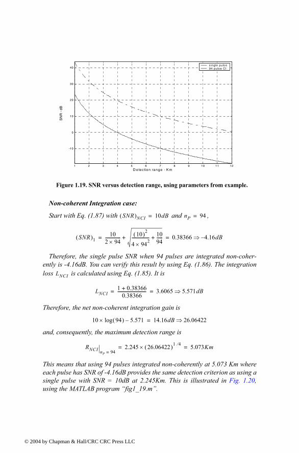
© 200
Non-coherent Integration case:
Start with Eq. (1.87) with and ,
Therefore, the single pulse SNR when 94 pulses are integrated non-coher-ently is -4.16dB. You can verify this result by using Eq. (1.86). The integration loss is calculated using Eq. (1.85). It is
Therefore, the net non-coherent integration gain is
and, consequently, the maximum detection range is
This means that using 94 pulses integrated non-coherently at 5.073 Km where each pulse has SNR of -4.16dB provides the same detection criterion as using a single pulse with SNR = 10dB at 2.245Km. This is illustrated in Fig. 1.20, using the MATLAB program fig1_19.m.
Figure 1.19. SNR versus detection range, using parameters from example.
1 2 3 4 5 6 7 8 9 10 11 12
-10
0
10
20
30
40
D etection range - K m
SN
R -
dBs ingle puls e94 puls e CI
SNR( )NCI 10dB= nP 94=
SNR( )110
2 94×--------------- 10( )2
4 942×----------------- 10
94------++ 0.38366 4.16dB⇒= =
LNCI
LNCI1 0.38366+
0.38366---------------------------- 3.6065 5.571dB⇒= =
10 94( )log× 5.571 14.16dB 26.06422⇒=
RNCI nP 94=2.245 26.06422( )1 4⁄× 5.073Km= =
4 by Chapman & Hall/CRC CRC Press LLC
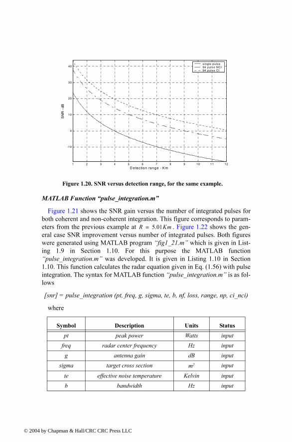
© 200
MATLAB Function pulse_integration.m
Figure 1.21 shows the SNR gain versus the number of integrated pulses for both coherent and non-coherent integration. This figure corresponds to param-eters from the previous example at . Figure 1.22 shows the gen-eral case SNR improvement versus number of integrated pulses. Both figures were generated using MATLAB program fig1_21.m which is given in List-ing 1.9 in Section 1.10. For this purpose the MATLAB function pulse_integration.m was developed. It is given in Listing 1.10 in Section 1.10. This function calculates the radar equation given in Eq. (1.56) with pulse integration. The syntax for MATLAB function pulse_integration.m is as fol-lows
[snr] = pulse_integration (pt, freq, g, sigma, te, b, nf, loss, range, np, ci_nci)
where
Symbol Description Units Status
pt peak power Watts input
freq radar center frequency Hz input
g antenna gain dB input
sigma target cross section m2 input
te effective noise temperature Kelvin input
b bandwidth Hz input
Figure 1.20. SNR versus detection range, for the same example.
1 2 3 4 5 6 7 8 9 10 11 12
-10
0
10
20
30
40
D etection range - K m
SN
R -
dBs ingle puls e94 pulse NCI94 pulse CI
R 5.01Km=
4 by Chapman & Hall/CRC CRC Press LLC
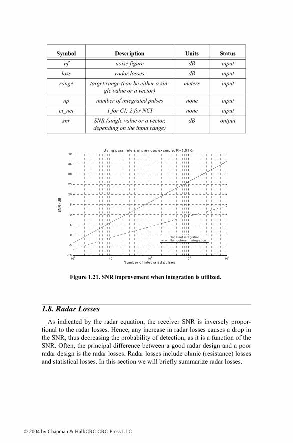
© 200
1.8. Radar LossesAs indicated by the radar equation, the receiver SNR is inversely propor-
tional to the radar losses. Hence, any increase in radar losses causes a drop in the SNR, thus decreasing the probability of detection, as it is a function of the SNR. Often, the principal difference between a good radar design and a poor radar design is the radar losses. Radar losses include ohmic (resistance) losses and statistical losses. In this section we will briefly summarize radar losses.
nf noise figure dB input
loss radar losses dB input
range target range (can be either a sin-gle value or a vector)
meters input
np number of integrated pulses none input
ci_nci 1 for CI; 2 for NCI none input
snr SNR (single value or a vector, depending on the input range)
dB output
Symbol Description Units Status
Figure 1.21. SNR improvement when integration is utilized.
100
101
102
103
104
-10
-5
0
5
10
15
20
25
30
35
40
N umber o f in tegrated pu lses
SN
R -
dB
U s ing parameters o f p revious exam ple, R =5.01K m
Coherent integrat ionNon-c oherent integrat ion
4 by Chapman & Hall/CRC CRC Press LLC
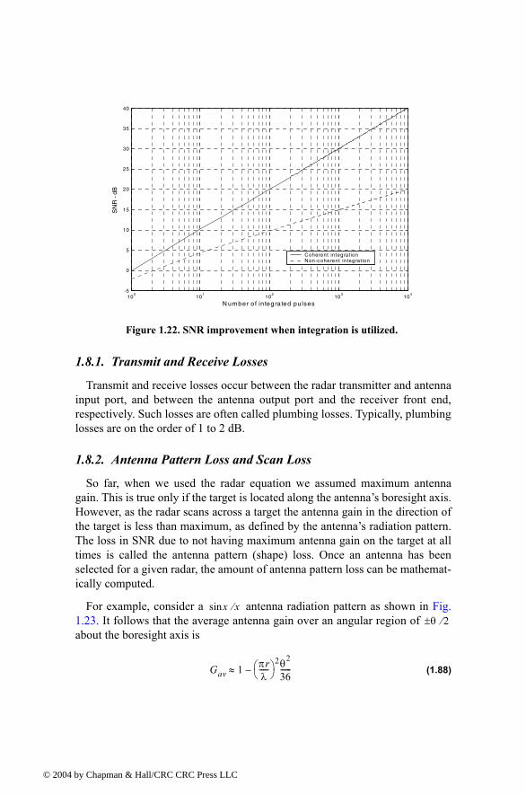
© 200
1.8.1. Transmit and Receive Losses
Transmit and receive losses occur between the radar transmitter and antenna input port, and between the antenna output port and the receiver front end, respectively. Such losses are often called plumbing losses. Typically, plumbing losses are on the order of 1 to 2 dB.
1.8.2. Antenna Pattern Loss and Scan Loss
So far, when we used the radar equation we assumed maximum antenna gain. This is true only if the target is located along the antennas boresight axis. However, as the radar scans across a target the antenna gain in the direction of the target is less than maximum, as defined by the antennas radiation pattern. The loss in SNR due to not having maximum antenna gain on the target at all times is called the antenna pattern (shape) loss. Once an antenna has been selected for a given radar, the amount of antenna pattern loss can be mathemat-ically computed.
For example, consider a antenna radiation pattern as shown in Fig. 1.23. It follows that the average antenna gain over an angular region of about the boresight axis is
(1.88)
Figure 1.22. SNR improvement when integration is utilized.
100
101
102
103
104
-5
0
5
10
15
20
25
30
35
40
N umber o f in tegrated pu lses
SN
R -
dB
Coherent integrat ionNon-coherent integrat ion
xsin x⁄θ 2⁄±
Gav 1 πrλ----- 2θ2
36------≈
4 by Chapman & Hall/CRC CRC Press LLC
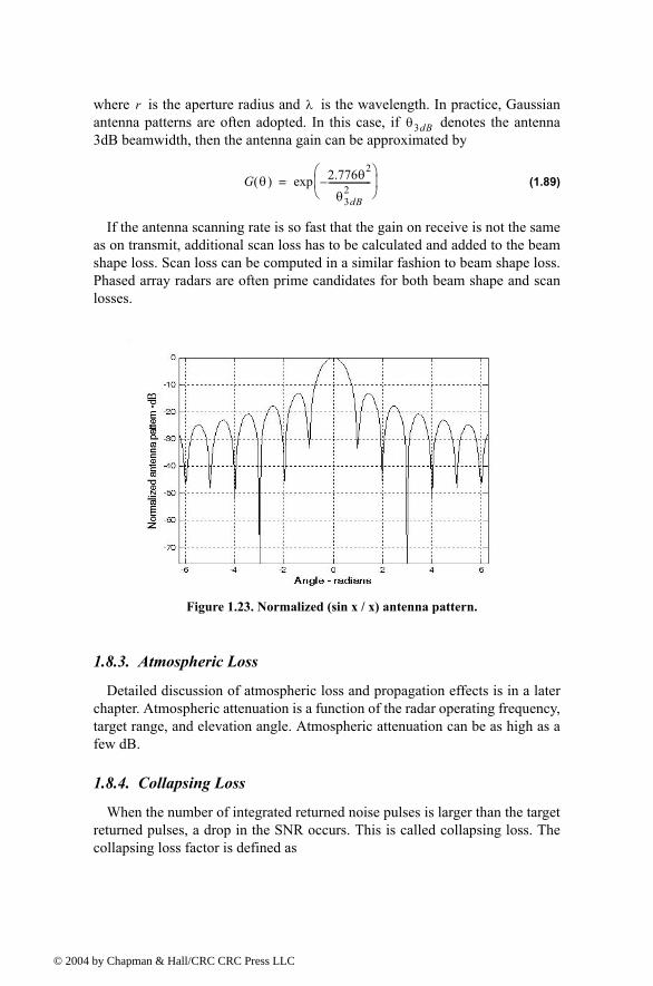
© 200
where is the aperture radius and is the wavelength. In practice, Gaussian antenna patterns are often adopted. In this case, if denotes the antenna 3dB beamwidth, then the antenna gain can be approximated by
(1.89)
If the antenna scanning rate is so fast that the gain on receive is not the same as on transmit, additional scan loss has to be calculated and added to the beam shape loss. Scan loss can be computed in a similar fashion to beam shape loss. Phased array radars are often prime candidates for both beam shape and scan losses.
1.8.3. Atmospheric Loss
Detailed discussion of atmospheric loss and propagation effects is in a later chapter. Atmospheric attenuation is a function of the radar operating frequency, target range, and elevation angle. Atmospheric attenuation can be as high as a few dB.
1.8.4. Collapsing Loss
When the number of integrated returned noise pulses is larger than the target returned pulses, a drop in the SNR occurs. This is called collapsing loss. The collapsing loss factor is defined as
r λθ3dB
G θ( ) 2.776θ2
θ3dB2
-------------------
exp=
Figure 1.23. Normalized (sin x / x) antenna pattern.
4 by Chapman & Hall/CRC CRC Press LLC
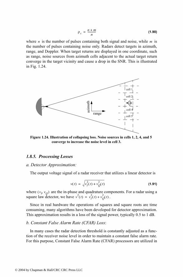
© 200
(1.90)
where is the number of pulses containing both signal and noise, while is the number of pulses containing noise only. Radars detect targets in azimuth, range, and Doppler. When target returns are displayed in one coordinate, such as range, noise sources from azimuth cells adjacent to the actual target return converge in the target vicinity and cause a drop in the SNR. This is illustrated in Fig. 1.24.
1.8.5. Processing Losses
a. Detector Approximation:
The output voltage signal of a radar receiver that utilizes a linear detector is
(1.91)
where are the in-phase and quadrature components. For a radar using a square law detector, we have .
Since in real hardware the operations of squares and square roots are time consuming, many algorithms have been developed for detector approximation. This approximation results in a loss of the signal power, typically 0.5 to 1 dB.
b. Constant False Alarm Rate (CFAR) Loss:
In many cases the radar detection threshold is constantly adjusted as a func-tion of the receiver noise level in order to maintain a constant false alarm rate. For this purpose, Constant False Alarm Rate (CFAR) processors are utilized in
ρcn m+
n-------------=
n m
cell 5
cell 4
cell 2
cell 1
rangeazim
uth
Figure 1.24. Illustration of collapsing loss. Noise sources in cells 1, 2, 4, and 5 converge to increase the noise level in cell 3.
v t( ) vI2 t( ) vQ
2 t( )+=
vI vQ,( )v2 t( ) vI
2 t( ) vQ2 t( )+=
4 by Chapman & Hall/CRC CRC Press LLC
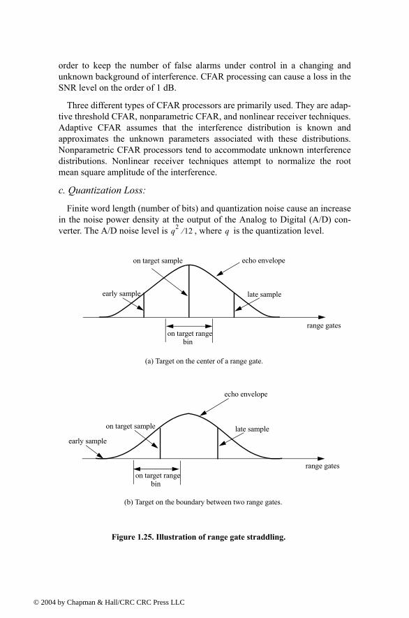
© 200
order to keep the number of false alarms under control in a changing and unknown background of interference. CFAR processing can cause a loss in the SNR level on the order of 1 dB.
Three different types of CFAR processors are primarily used. They are adap-tive threshold CFAR, nonparametric CFAR, and nonlinear receiver techniques. Adaptive CFAR assumes that the interference distribution is known and approximates the unknown parameters associated with these distributions. Nonparametric CFAR processors tend to accommodate unknown interference distributions. Nonlinear receiver techniques attempt to normalize the root mean square amplitude of the interference.
c. Quantization Loss:
Finite word length (number of bits) and quantization noise cause an increase in the noise power density at the output of the Analog to Digital (A/D) con-verter. The A/D noise level is , where is the quantization level.q2 12⁄ q
echo envelope
early sample late sample
on target sample
on target rangebin
echo envelope
early samplelate sampleon target sample
on target rangebin
(a) Target on the center of a range gate.
range gates
range gates
(b) Target on the boundary between two range gates.
Figure 1.25. Illustration of range gate straddling.
4 by Chapman & Hall/CRC CRC Press LLC
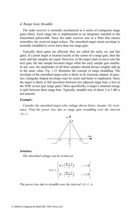
© 200
d. Range Gate Straddle:
The radar receiver is normally mechanized as a series of contiguous range gates (bins). Each range bin is implemented as an integrator matched to the transmitted pulsewidth. Since the radar receiver acts as a filter that smears (smooths), the received target echoes. The smoothed target return envelope is normally straddled to cover more than one range gate.
Typically, three gates are affected; they are called the early, on, and late gates. If a point target is located exactly at the center of a range gate, then the early and late samples are equal. However, as the target starts to move into the next gate, the late sample becomes larger while the early sample gets smaller. In any case, the amplitudes of all three samples should always roughly add up to the same value. Fig. 1.25 illustrates the concept of range straddling. The envelope of the smoothed target echo is likely to be Gaussian shaped. In prac-tice, triangular shaped envelopes may be easier and faster to implement. Since the target is likely to fall anywhere between two adjacent range bins, a loss in the SNR occurs (per range gate). More specifically, a targets returned energy is split between three range bins. Typically, straddle loss of about 2 to 3 dB is not unusual.
Example:
Consider the smoothed target echo voltage shown below. Assume resis-tance. Find the power loss due to range gate straddling over the interval
.
Solution: The smoothed voltage can be written as
The power loss due to straddle over the interval is
1Ω
0 τ,
0τ τtime
Kv(t)
-1
v t( )K K 1+
τ------------- t+ t 0<;
K K 1+τ
------------- t t 0≥;
=
0 τ,
4 by Chapman & Hall/CRC CRC Press LLC
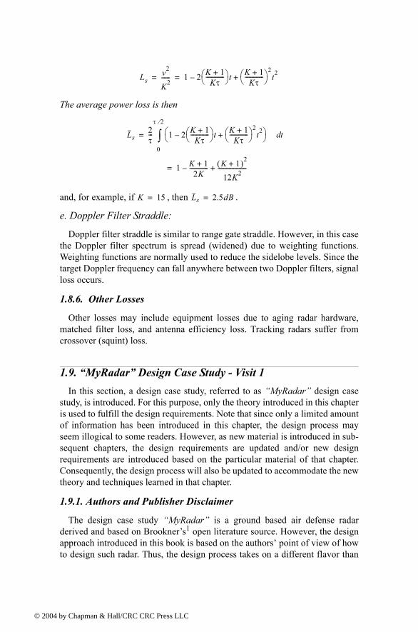
© 200
The average power loss is then
and, for example, if , then .
e. Doppler Filter Straddle:
Doppler filter straddle is similar to range gate straddle. However, in this case the Doppler filter spectrum is spread (widened) due to weighting functions. Weighting functions are normally used to reduce the sidelobe levels. Since the target Doppler frequency can fall anywhere between two Doppler filters, signal loss occurs.
1.8.6. Other Losses
Other losses may include equipment losses due to aging radar hardware, matched filter loss, and antenna efficiency loss. Tracking radars suffer from crossover (squint) loss.
1.9. MyRadar Design Case Study - Visit 1In this section, a design case study, referred to as MyRadar design case
study, is introduced. For this purpose, only the theory introduced in this chapter is used to fulfill the design requirements. Note that since only a limited amount of information has been introduced in this chapter, the design process may seem illogical to some readers. However, as new material is introduced in sub-sequent chapters, the design requirements are updated and/or new design requirements are introduced based on the particular material of that chapter. Consequently, the design process will also be updated to accommodate the new theory and techniques learned in that chapter.
1.9.1. Authors and Publisher Disclaimer
The design case study MyRadar is a ground based air defense radar derived and based on Brookners1 open literature source. However, the design approach introduced in this book is based on the authors point of view of how to design such radar. Thus, the design process takes on a different flavor than
Lsv2
K2------ 1 2 K 1+
Kτ------------- t
K 1+Kτ
------------- 2
t2+= =
Ls2τ--- 1 2 K 1+
Kτ------------- t
K 1+Kτ
------------- 2
t2+
td0
τ 2⁄
∫
1 K 1+2K
------------- K 1+( )2
12K2--------------------+
=
=
K 15= Ls 2.5dB=
4 by Chapman & Hall/CRC CRC Press LLC
© 200
that introduced by Brookner. Additionally, any and all design alternatives pre-sented in this book are based on and can be easily traced to open literature sources.
Furthermore, the design approach adopted in this book is based on modeling many of the radar system components with no regards to any hardware con-straints nor to any practical limitations. The design presented in this book is intended to be tutorial and academic in nature and does not adhere to any other requirements. Finally, the MATLAB code presented in this book is intended to be illustrative and academic and is not designed nor intended for any other uses.
Using the material presented in this book and the MATLAB code designed by the authors of this book by any entity or person is strictly at will. The authors and the publisher are neither liable nor responsible for any material or non-material losses, loss of wages, personal or property damages of any kind, or for any other type of damages of any and all types that may be incurred by using this book.
1.9.2. Problem Statement
You are to design a ground based radar to fulfill the following mission: Search and Detection. The threat consists of aircraft with an average RCS of 6 dBsm ( ), and missiles with an average RCS of -3 dBsm ( ). The missile altitude is 2Km, and the aircraft altitude is about 7 Km. Assume a scanning radar with 360 degrees azimuth coverage. The scan rate is less than or equal to 1 revolution every 2 seconds. Assume L to X band. We need range resolution of 150 m. No angular resolution is specified at this time. Also assume that only one missile and one aircraft constitute the whole threat. Assume a noise figure F = 6 dB, and total receiver loss L = 8 dB. For now use a fan beam with azimuth beamwidth of less than 3 degrees. Assume that 13 dB SNR is a reasonable detection threshold. Finally, assume flat earth.
1.9.3. A Design
The desired range resolution is . Thus, using Eq. (1.8) one calcu-lates the required pulsewidth as , or equivalently the required band-width . At this point a few preliminary decisions must be made. This includes the selection of the radar operating frequency, the aperture size, and the single pulse peak power.
1. Brookner, Eli, Editor, Practical Phased Array Antenna Systems, Artech House, 1991, Chapter 7.
σa 4m2=
σm 0.5m2=
∆R 150m=τ 1µ sec=
B 1MHz=
4 by Chapman & Hall/CRC CRC Press LLC
© 200
The choice of an operating frequency that can fulfill the design requirements is driven by many factors, such as aperture size, antenna gain, clutter, atmo-spheric attenuation, and the maximum peak power, to name a few. In this design, an operating frequency is selected. This choice is somewhat arbitrary at this point; however, as we proceed with the design process this choice will be better clarified.
Second, the transportability (mobility) of the radar drives the designer in the direction of a smaller aperture type. A good choice would be less than 5 meters squared. For now choose . The last issue that one must consider is the energy required per pulse. Note that this design approach assumes that the minimum detection SNR (13 dB) requirement is based on pulse integration. This condition is true because the target is illuminated with several pulses dur-ing a single scan, provided that the antenna azimuth beamwidth and the PRF choice satisfy Eq. (1.81).
The single pulse energy is . Typically, a given radar must be designed such that it has a handful of pulsewidths (waveforms) to choose from. Different waveforms (pulsewidths) are used for definite modes of operations (search, track, etc.). However, for now only a single pulse which satisfies the range resolution requirement is considered. To calculate the minimum single pulse energy required for proper detection, use Eq. (1.57). More precisely,
(1.92)
All parameters in Eq. (1.92) are known, except for the antenna gain, the detec-tion range, and the single pulse SNR. The antenna gain is calculated from
(1.93)
where the relation ( ) was used.
In order to estimate the detection range, consider the following argument. Since an aircraft has a larger RCS than a missile, one would expect an aircraft to be detected at a much longer range than that of a missile. This is depicted in Fig. 1.26, where refers to the aircraft detection range and denotes the missile detection range. As illustrated in this figure, the minimum search ele-vation angle is driven by the missile detection range, assuming that the mis-siles are detected, with the proper SNR, as soon as they enter the radar beam. Alternatively, the maximum search elevation angle is driven the aircrafts position along with the range that corresponds to the defenses last chance to intercept the threat (both aircraft and missile). This range is often called keep-out minimum range and is denoted by . In this design approach,
f 3GHz=
Ae 2.25m2=
E Ptτ=
E Ptτ4π( )3kTeFLR4SNR1
G2λ2σ---------------------------------------------------= =
G4πAe
λ2------------ 4π 2.25×
0.1( )2----------------------- 2827.4= = =
G⇒ 34.5dB=
λ c f⁄=
Ra Rm
θ1
θ2
Rmin
4 by Chapman & Hall/CRC CRC Press LLC
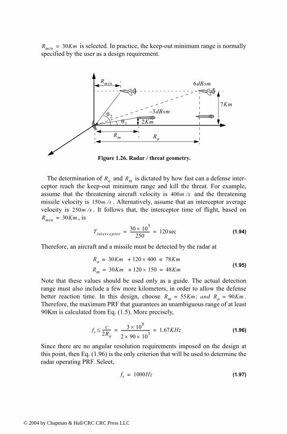
© 200
is selected. In practice, the keep-out minimum range is normally specified by the user as a design requirement.
The determination of and is dictated by how fast can a defense inter-ceptor reach the keep-out minimum range and kill the threat. For example, assume that the threatening aircraft velocity is and the threatening missile velocity is . Alternatively, assume that an interceptor average velocity is . It follows that, the interceptor time of flight, based on
, is
(1.94)
Therefore, an aircraft and a missile must be detected by the radar at
(1.95)
Note that these values should be used only as a guide. The actual detection range must also include a few more kilometers, in order to allow the defense better reaction time. In this design, choose . Therefore, the maximum PRF that guarantees an unambiguous range of at least 90Km is calculated from Eq. (1.5). More precisely,
(1.96)
Since there are no angular resolution requirements imposed on the design at this point, then Eq. (1.96) is the only criterion that will be used to determine the radar operating PRF. Select,
(1.97)
Rmin 30Km=
θ2θ1
Figure 1.26. Radar / threat geometry.
2Km
7Km
6dBsm
3dBsm
Rm Ra
Rmin
Ra Rm
400m s⁄150m s⁄
250m s⁄Rmin 30Km=
Tinterceptor30 103×
250-------------------- 120sec= =
Ra 30Km 120 400×+ 78Km= =
Rm 30Km 120 150×+ 48Km= =
Rm 55Km and Ra; 90Km= =
frc
2Ru---------≤ 3 108×
2 90 103××------------------------------ 1.67KHz= =
fr 1000Hz=
4 by Chapman & Hall/CRC CRC Press LLC
© 200
The minimum and maximum elevation angles are, respectively, calculated as
(1.98)
(1.99)
These angles are then used to compute the elevation search extent (remember that the azimuth search extent is equal to ). More precisely, the search vol-ume (in steradians) is given by
(1.100)
Consequently, the search volume is
(1.101)
The desired antenna must have a fan beam; thus using a parabolic rectangu-lar antenna will meet the design requirements. Select ; the corre-sponding antenna 3-dB elevation and azimuth beamwidths are denoted as
, respectively. Select
(1.102)
The azimuth 3-dB antenna beamwidth is calculated using Eq. (1.42) as
(1.103)
It follows that the number of pulses that strikes a target during a single scan is calculated using Eq. (1.81) as
(1.104)
The design approach presented in this book will only assume non-coherent integration (the reader is advised to re-calculate all results by assuming coher-ent integration, instead). The design requirement mandates a 13 dB SNR for detection. By using Eq. (1.87) one calculates the required single pulse SNR,
(1.105)
θ12
55------ atan 2.08°= =
θ2730------ atan 13.13°= =
360°Ω
Ωθ2 θ1
57.296( )2----------------------- 360×=
Ω 360θ2 θ1
57.296( )2-----------------------× 360 13.13 2.08
57.296( )2------------------------------× 1.212 steradians= = =
Ae 2.25m2=
θe θa,
θe θ2 θ1 13.13 2.08 11.05°= = =
θa4π
Gθe---------- 4 π× 1802×
2827.4 π2 11××---------------------------------------- 1.33°= = =
npθafr
θ· scan------------≤ 1.33 1000×
180---------------------------- 7.39 np⇒ 7= = =
SNR( )1101.3
2 7×------------ 101.3( )
2
4 72×------------------- 101.3
7------------++ 3.635= = SNR( )1⇒ 5.6dB=
4 by Chapman & Hall/CRC CRC Press LLC
© 200
Furthermore the non-coherent integration loss associated with this case is com-puted from Eq. (1.85),
(1.106)
It follows that the corresponding single pulse energy for the missile and the aircraft cases are respectively given by
(1.107)
(1.108)
Hence, the peak power that satisfies the single pulse detection requirement for both target types is
(1.109)
The radar equation with pulse integration is
(1.110)
Figure 1.27 shows the SNR versus detection range for both target-types with and without integration. To reproduce this figure use MATLAB program fig1_27.m which is given in Listing 1.12 in Section 1.10.
1.9.4. A Design Alternative
One could have elected not to reduce the single pulse peak power, but rather keep the single pulse peak power as computed in Eq. (1.109) and increase the radar detection range. For example, integrating 7 pulses coherently would improve the radar detection range by a factor of
(1.111)
LNCI1 3.635+
3.635---------------------- 1.27= = LNCI⇒ 1.056dB=
Em4π( )3kTeFLRm
4 SNR( )1
G2λ2σm
---------------------------------------------------------= ⇒
Em4π( )3 1.38 10 23×( ) 290( ) 100.8( ) 100.6( ) 55 103×( )
4100.56
2827.4( )2 0.1( )2 0.5( )--------------------------------------------------------------------------------------------------------------------------------------------- 0.1658 Joules= =
Ea4π( )3kTeFLRa
4 SNR( )1
G2λ2σa
--------------------------------------------------------= ⇒
Ea4π( )3 1.38 10 23×( ) 290( ) 100.8( ) 100.6( ) 90 103×( )
4100.56
2827.4( )2 0.1( )2 4( )--------------------------------------------------------------------------------------------------------------------------------------------- 0.1487 Joules= =
PtEτ--- 0.1658
1 10 6×-------------------- 165.8KW= = =
SNRPt
1G2λ2σ
4π( )3kTeBFLR4-----------------------------------------
npLNCI------------=
Rimp 7( )0.25 1.63= =
4 by Chapman & Hall/CRC CRC Press LLC
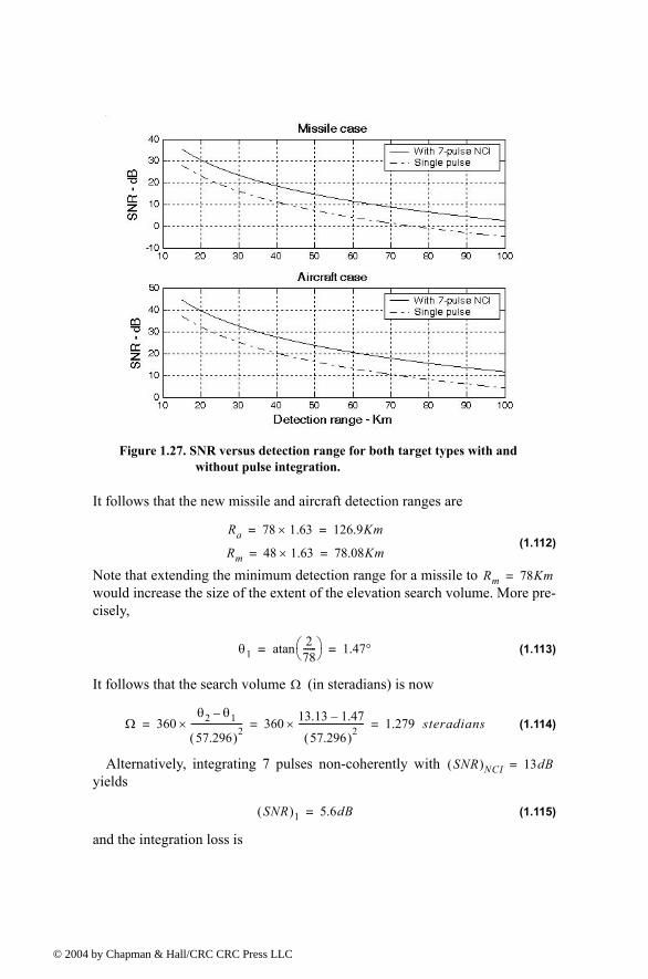
© 200
It follows that the new missile and aircraft detection ranges are
(1.112)
Note that extending the minimum detection range for a missile to would increase the size of the extent of the elevation search volume. More pre-cisely,
(1.113)
It follows that the search volume (in steradians) is now
(1.114)
Alternatively, integrating 7 pulses non-coherently with yields
(1.115)
and the integration loss is
Figure 1.27. SNR versus detection range for both target types with and without pulse integration.
Ra 78 1.63× 126.9Km= =
Rm 48 1.63× 78.08Km= =
Rm 78Km=
θ12
78------ atan 1.47°= =
Ω
Ω 360θ2 θ1
57.296( )2-----------------------× 360 13.13 1.47
57.296( )2------------------------------× 1.279 steradians= = =
SNR( )NCI 13dB=
SNR( )1 5.6dB=
4 by Chapman & Hall/CRC CRC Press LLC
© 200
(1.116)
Then, the net non-coherent integration gain is
(1.117)
Thus, the radar detection range is now improved due to a 7-pulse non-coherent integration to
(1.118)
Again, the extent of the elevation search volume is changed to
(1.119)
It follows that the search volume (in steradians) is now
(1.120)
1.10. MATLAB Program and Function ListingsThis section presents listings for all MATLAB functions and programs used
in this chapter. Users are encouraged to vary the input parameters and rerun these programs in order to enhance their understanding of the theory presented in the text. All selected parameters and variables follow the same nomenclature used in the text; thus, understanding the structure and hierarchy of the pre-sented code should be an easy task once the user has read the chapter.
Note that all MATLAB programs and functions developed in this book can be downloaded from CRC Press Web Site www.crcpress.com. Additionally, all MATLAB code developed for this book was developed using MATLAB 6.5 Release 13 for Microsoft Windows.
Listing 1.1. MATLAB Function radar_eq.mfunction [snr] = radar_eq(pt, freq, g, sigma, te, b, nf, loss, range)% This program implements Eq. (1.56)c = 3.0e+8; % speed of lightlambda = c / freq; % wavelengthp_peak = 10*log10(pt); % convert peak power to dBlambda_sqdb = 10*log10(lambda^2); % compute wavelength square in dBsigmadb = 10*log10(sigma); % convert sigma to dBfour_pi_cub = 10*log10((4.0 * pi)^3); % (4pi)^3 in dB
LNCI 1.057dB=
NCIgain 10 7( )log× 1.057 7.394dB= = NCIgain⇒ 5.488=
Ra 78 5.488( )0.25× 119.38Km= =
Rm 48 5.488( )0.25× 73.467Km= =
θ12
73.467---------------- atan 1.56°= =
Ω
Ω 360θ2 θ1
57.296( )2-----------------------× 360 13.13 1.56
57.296( )2------------------------------× 1.269 steradians= = =
4 by Chapman & Hall/CRC CRC Press LLC
© 200
k_db = 10*log10(1.38e-23); % Boltzman's constant in dBte_db = 10*log10(te); % noise temp. in dBb_db = 10*log10(b); % bandwidth in dBrange_pwr4_db = 10*log10(range.^4); % vector of target range^4 in dB% Implement Equation (1.56)num = p_peak + g + g + lambda_sqdb + sigmadb;den = four_pi_cub + k_db + te_db + b_db + nf + loss + range_pwr4_db;snr = num - den;return
Listing 1.2. MATLAB Program fig1_12.m% Use this program to reproduce Fig. 1.12 of text.close allclear allpt = 1.5e+6; % peak power in Wattsfreq = 5.6e+9; % radar operating frequency in Hzg = 45.0; % antenna gain in dBsigma = 0.1; % radar cross section in m squaredte = 290.0; % effective noise temperature in Kelvinsb = 5.0e+6; % radar operating bandwidth in Hznf = 3.0; %noise figure in dBloss = 6.0; % radar losses in dBrange = linspace(25e3,165e3,1000); % traget range 25 -165 Km, 1000 pointssnr1 = radar_eq(pt, freq, g, sigma, te, b, nf, loss, range);snr2 = radar_eq(pt, freq, g, sigma/10, te, b, nf, loss, range);snr3 = radar_eq(pt, freq, g, sigma*10, te, b, nf, loss, range);% plot SNR versus rangefigure(1)rangekm = range ./ 1000;plot(rangekm,snr3,'k',rangekm,snr1,'k -.',rangekm,snr2,'k:')gridlegend('\sigma = 0 dBsm','\sigma = -10dBsm','\sigma = -20 dBsm')xlabel ('Detection range - Km');ylabel ('SNR - dB');snr1 = radar_eq(pt, freq, g, sigma, te, b, nf, loss, range);snr2 = radar_eq(pt*.4, freq, g, sigma, te, b, nf, loss, range);snr3 = radar_eq(pt*1.8, freq, g, sigma, te, b, nf, loss, range);figure (2)plot(rangekm,snr3,'k',rangekm,snr1,'k -.',rangekm,snr2,'k:')gridlegend('Pt = 2.16 MW','Pt = 1.5 MW','Pt = 0.6 MW')xlabel ('Detection range - Km');ylabel ('SNR - dB');
4 by Chapman & Hall/CRC CRC Press LLC
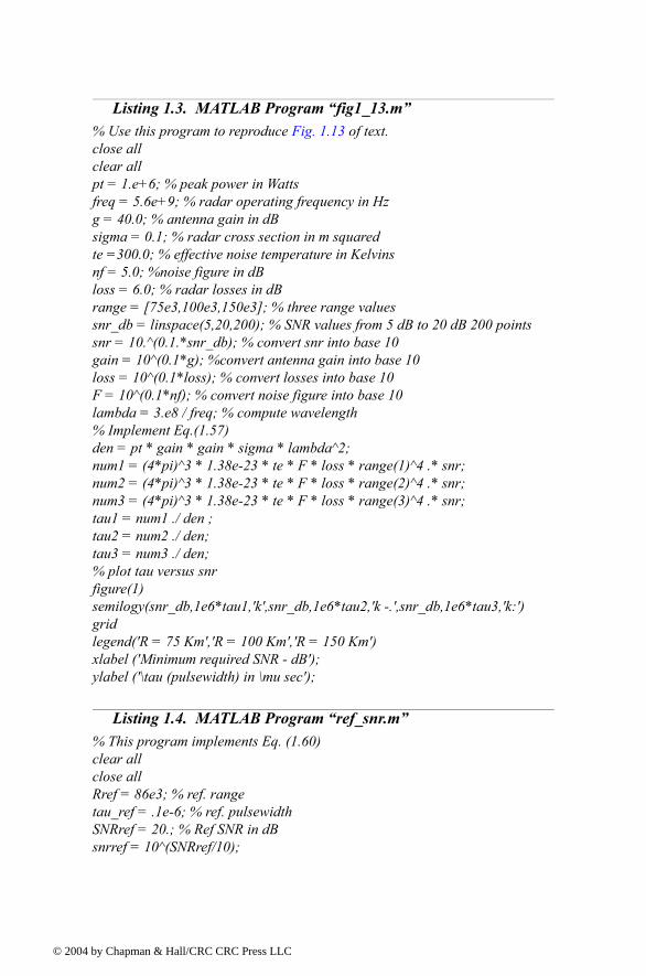
© 200
Listing 1.3. MATLAB Program fig1_13.m% Use this program to reproduce Fig. 1.13 of text.close allclear allpt = 1.e+6; % peak power in Wattsfreq = 5.6e+9; % radar operating frequency in Hzg = 40.0; % antenna gain in dBsigma = 0.1; % radar cross section in m squaredte =300.0; % effective noise temperature in Kelvinsnf = 5.0; %noise figure in dBloss = 6.0; % radar losses in dBrange = [75e3,100e3,150e3]; % three range valuessnr_db = linspace(5,20,200); % SNR values from 5 dB to 20 dB 200 pointssnr = 10.^(0.1.*snr_db); % convert snr into base 10gain = 10^(0.1*g); %convert antenna gain into base 10loss = 10^(0.1*loss); % convert losses into base 10F = 10^(0.1*nf); % convert noise figure into base 10lambda = 3.e8 / freq; % compute wavelength% Implement Eq.(1.57)den = pt * gain * gain * sigma * lambda^2;num1 = (4*pi)^3 * 1.38e-23 * te * F * loss * range(1)^4 .* snr;num2 = (4*pi)^3 * 1.38e-23 * te * F * loss * range(2)^4 .* snr;num3 = (4*pi)^3 * 1.38e-23 * te * F * loss * range(3)^4 .* snr;tau1 = num1 ./ den ;tau2 = num2 ./ den;tau3 = num3 ./ den;% plot tau versus snrfigure(1)semilogy(snr_db,1e6*tau1,'k',snr_db,1e6*tau2,'k -.',snr_db,1e6*tau3,'k:')gridlegend('R = 75 Km','R = 100 Km','R = 150 Km')xlabel ('Minimum required SNR - dB');ylabel ('\tau (pulsewidth) in \mu sec');
Listing 1.4. MATLAB Program ref_snr.m% This program implements Eq. (1.60)clear allclose allRref = 86e3; % ref. rangetau_ref = .1e-6; % ref. pulsewidthSNRref = 20.; % Ref SNR in dBsnrref = 10^(SNRref/10);
4 by Chapman & Hall/CRC CRC Press LLC
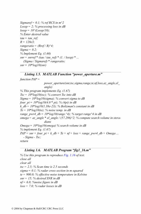
© 200
Sigmaref = 0.1; % ref RCS in m^2Lossp = 2; % processing loss in dBlossp = 10^(Lossp/10);% Enter desired valuetau = tau_ref;R = 120e3;rangeratio = (Rref / R)^4;Sigma = 0.2; % Implement Eq. (1.60)snr = snrref * (tau / tau_ref) * (1. / lossp) * ... (Sigma / Sigmaref) * rangeratio;snr = 10*log10(snr)
Listing 1.5. MATLAB Function power_aperture.mfunction PAP =
power_aperture(snr,tsc,sigma,range,te,nf,loss,az_angle,el_angle)
% This program implements Eq. (1.67)Tsc = 10*log10(tsc); % convert Tsc into dBSigma = 10*log10(sigma); % convert sigma to dBfour_pi = 10*log10(4.0 * pi); % (4pi) in dBk_db = 10*log10(1.38e-23); % Boltzman's constant in dBTe = 10*log10(te); % noise temp. in dBrange_pwr4_db = 10*log10(range.^4); % target range^4 in dBomega = az_angle * el_angle / (57.296)^2; % compute search volume in stera-
diansOmega = 10*log10(omega) % search volume in dB% implement Eq. (1.67)PAP = snr + four_pi + k_db + Te + nf + loss + range_pwr4_db + Omega ... - Sigma - Tsc;return
Listing 1.6. MATLAB Program fig1_16.m% Use this program to reproduce Fig. 1.16 of text.close allclear alltsc = 2.5; % Scan time is 2.5 secondssigma = 0.1; % radar cross section in m squaredte = 900.0; % effective noise temperature in Kelvinssnr = 15; % desired SNR in dBnf = 6.0; %noise figure in dBloss = 7.0; % radar losses in dB
4 by Chapman & Hall/CRC CRC Press LLC
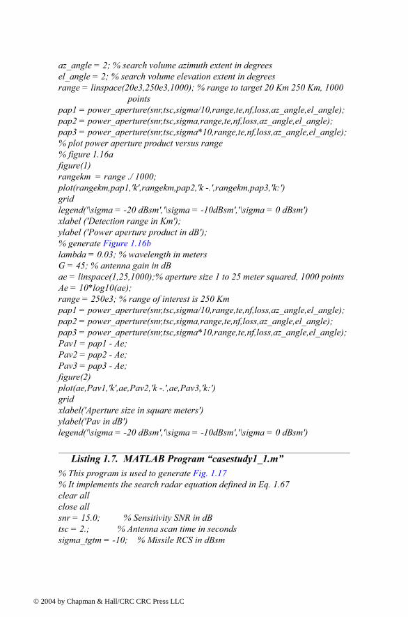
© 200
az_angle = 2; % search volume azimuth extent in degreesel_angle = 2; % search volume elevation extent in degreesrange = linspace(20e3,250e3,1000); % range to target 20 Km 250 Km, 1000
pointspap1 = power_aperture(snr,tsc,sigma/10,range,te,nf,loss,az_angle,el_angle);pap2 = power_aperture(snr,tsc,sigma,range,te,nf,loss,az_angle,el_angle);pap3 = power_aperture(snr,tsc,sigma*10,range,te,nf,loss,az_angle,el_angle);% plot power aperture product versus range% figure 1.16afigure(1)rangekm = range ./ 1000;plot(rangekm,pap1,'k',rangekm,pap2,'k -.',rangekm,pap3,'k:')gridlegend('\sigma = -20 dBsm','\sigma = -10dBsm','\sigma = 0 dBsm')xlabel ('Detection range in Km');ylabel ('Power aperture product in dB');% generate Figure 1.16blambda = 0.03; % wavelength in metersG = 45; % antenna gain in dBae = linspace(1,25,1000);% aperture size 1 to 25 meter squared, 1000 pointsAe = 10*log10(ae);range = 250e3; % range of interest is 250 Kmpap1 = power_aperture(snr,tsc,sigma/10,range,te,nf,loss,az_angle,el_angle);pap2 = power_aperture(snr,tsc,sigma,range,te,nf,loss,az_angle,el_angle);pap3 = power_aperture(snr,tsc,sigma*10,range,te,nf,loss,az_angle,el_angle);Pav1 = pap1 - Ae;Pav2 = pap2 - Ae;Pav3 = pap3 - Ae;figure(2)plot(ae,Pav1,'k',ae,Pav2,'k -.',ae,Pav3,'k:')gridxlabel('Aperture size in square meters')ylabel('Pav in dB')legend('\sigma = -20 dBsm','\sigma = -10dBsm','\sigma = 0 dBsm')
Listing 1.7. MATLAB Program casestudy1_1.m% This program is used to generate Fig. 1.17 % It implements the search radar equation defined in Eq. 1.67clear allclose allsnr = 15.0; % Sensitivity SNR in dBtsc = 2.; % Antenna scan time in secondssigma_tgtm = -10; % Missile RCS in dBsm
4 by Chapman & Hall/CRC CRC Press LLC
© 200
sigma_tgta = 6; % Aircraft RCS in dBsmrange = 60.0; % Sensitivity range in Km, te = 290.0; % Effective noise temperature in Kelvinsnf = 8; % Noise figure in dBloss = 10.0; % Radar losses in dBaz_angle = 360.0; % Search volume azimuth extent in degreesel_angle = 10.0; % Search volume elevation extent in degreesc = 3.0e+8; % Speed of light% Compute Omega in steradiansomega = (az_angle / 57.296) * (el_angle /57.296);omega_db = 10.0*log10(omega); % Convert Omega to dBsk_db = 10.*log10(1.38e-23);te_db = 10*log10(te);tsc_db = 10*log10(tsc);factor = 10*log10(4*pi);rangemdb = 10*log10(range * 1000.);rangeadb = 10*log10(range * 1000.);PAP_Missile = snr - sigma_tgtm - tsc_db + factor + 4.0 * rangemdb + ... k_db + te_db + nf + loss + omega_dbPAP_Aircraft = snr - sigma_tgta - tsc_db + factor + 4.0 * rangeadb + ... k_db + te_db + nf + loss + omega_dbindex = 0;% vary range from 2Km to 90 Km for rangevar = 2 : 1 : 90 index = index + 1; rangedb = 10*log10(rangevar * 1000.0); papm(index) = snr - sigma_tgtm - tsc_db + factor + 4.0 * rangedb + ... k_db + te_db + nf + loss + omega_db; missile_PAP(index) = PAP_Missile; aircraft_PAP(index) = PAP_Aircraft; papa(index) = snr - sigma_tgta - tsc_db + factor + 4.0 * rangedb + ... k_db + te_db + nf + loss +omega_db;endvar = 2 : 1 : 90;figure (1)plot (var,papm,'k',var,papa,'k-.')legend ('Missile','Aircraft')xlabel ('Range - Km');ylabel ('Power Aperture Product - dB');hold onplot(var,missile_PAP,'k:',var,aircraft_PAP,'k:')gridhold off
4 by Chapman & Hall/CRC CRC Press LLC
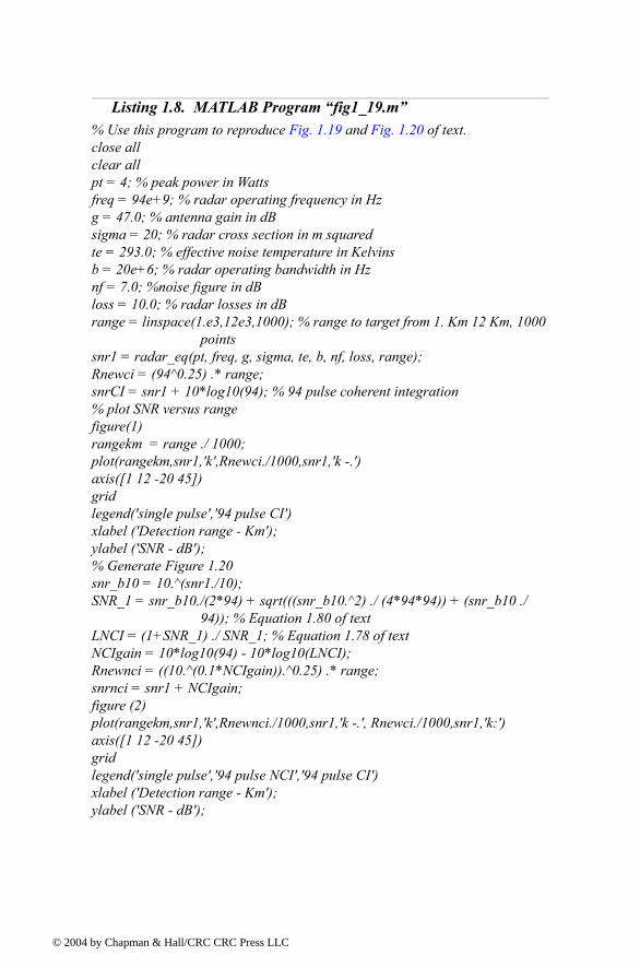
© 200
Listing 1.8. MATLAB Program fig1_19.m% Use this program to reproduce Fig. 1.19 and Fig. 1.20 of text.close allclear allpt = 4; % peak power in Wattsfreq = 94e+9; % radar operating frequency in Hzg = 47.0; % antenna gain in dBsigma = 20; % radar cross section in m squaredte = 293.0; % effective noise temperature in Kelvinsb = 20e+6; % radar operating bandwidth in Hznf = 7.0; %noise figure in dBloss = 10.0; % radar losses in dBrange = linspace(1.e3,12e3,1000); % range to target from 1. Km 12 Km, 1000
pointssnr1 = radar_eq(pt, freq, g, sigma, te, b, nf, loss, range);Rnewci = (94^0.25) .* range;snrCI = snr1 + 10*log10(94); % 94 pulse coherent integration% plot SNR versus rangefigure(1)rangekm = range ./ 1000;plot(rangekm,snr1,'k',Rnewci./1000,snr1,'k -.')axis([1 12 -20 45])gridlegend('single pulse','94 pulse CI')xlabel ('Detection range - Km');ylabel ('SNR - dB');% Generate Figure 1.20snr_b10 = 10.^(snr1./10);SNR_1 = snr_b10./(2*94) + sqrt(((snr_b10.^2) ./ (4*94*94)) + (snr_b10 ./
94)); % Equation 1.80 of textLNCI = (1+SNR_1) ./ SNR_1; % Equation 1.78 of textNCIgain = 10*log10(94) - 10*log10(LNCI);Rnewnci = ((10.^(0.1*NCIgain)).^0.25) .* range;snrnci = snr1 + NCIgain;figure (2)plot(rangekm,snr1,'k',Rnewnci./1000,snr1,'k -.', Rnewci./1000,snr1,'k:')axis([1 12 -20 45])gridlegend('single pulse','94 pulse NCI','94 pulse CI')xlabel ('Detection range - Km');ylabel ('SNR - dB');
4 by Chapman & Hall/CRC CRC Press LLC
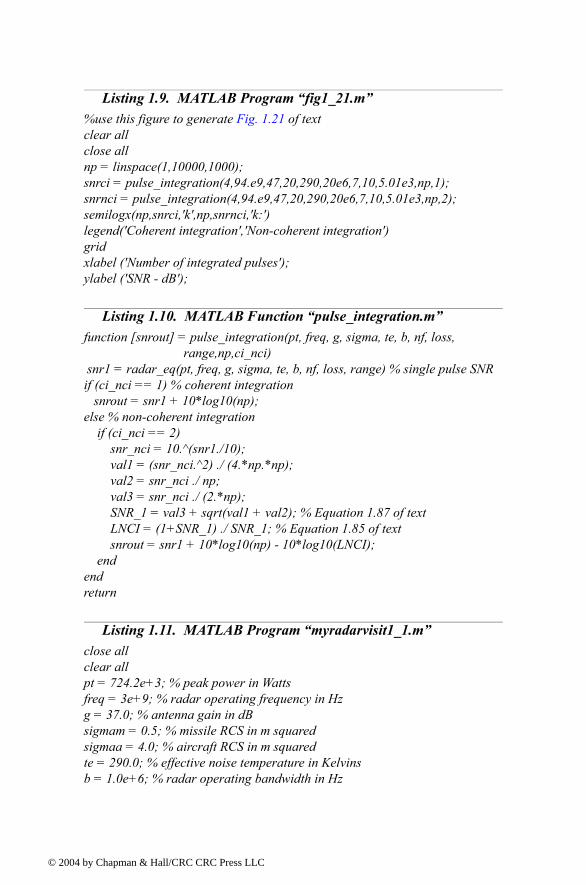
© 200
Listing 1.9. MATLAB Program fig1_21.m%use this figure to generate Fig. 1.21 of textclear allclose allnp = linspace(1,10000,1000);snrci = pulse_integration(4,94.e9,47,20,290,20e6,7,10,5.01e3,np,1);snrnci = pulse_integration(4,94.e9,47,20,290,20e6,7,10,5.01e3,np,2);semilogx(np,snrci,'k',np,snrnci,'k:')legend('Coherent integration','Non-coherent integration')gridxlabel ('Number of integrated pulses');ylabel ('SNR - dB');
Listing 1.10. MATLAB Function pulse_integration.mfunction [snrout] = pulse_integration(pt, freq, g, sigma, te, b, nf, loss,
range,np,ci_nci) snr1 = radar_eq(pt, freq, g, sigma, te, b, nf, loss, range) % single pulse SNRif (ci_nci == 1) % coherent integration snrout = snr1 + 10*log10(np);else % non-coherent integration if (ci_nci == 2) snr_nci = 10.^(snr1./10); val1 = (snr_nci.^2) ./ (4.*np.*np); val2 = snr_nci ./ np; val3 = snr_nci ./ (2.*np); SNR_1 = val3 + sqrt(val1 + val2); % Equation 1.87 of text LNCI = (1+SNR_1) ./ SNR_1; % Equation 1.85 of text snrout = snr1 + 10*log10(np) - 10*log10(LNCI); endendreturn
Listing 1.11. MATLAB Program myradarvisit1_1.mclose allclear allpt = 724.2e+3; % peak power in Wattsfreq = 3e+9; % radar operating frequency in Hzg = 37.0; % antenna gain in dBsigmam = 0.5; % missile RCS in m squaredsigmaa = 4.0; % aircraft RCS in m squaredte = 290.0; % effective noise temperature in Kelvinsb = 1.0e+6; % radar operating bandwidth in Hz
4 by Chapman & Hall/CRC CRC Press LLC
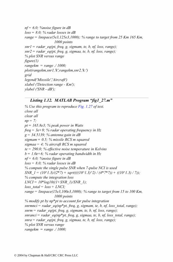
© 200
nf = 6.0; %noise figure in dBloss = 8.0; % radar losses in dBrange = linspace(5e3,125e3,1000); % range to target from 25 Km 165 Km,
1000 pointssnr1 = radar_eq(pt, freq, g, sigmam, te, b, nf, loss, range);snr2 = radar_eq(pt, freq, g, sigmaa, te, b, nf, loss, range);% plot SNR versus rangefigure(1)rangekm = range ./ 1000;plot(rangekm,snr1,'k',rangekm,snr2,'k:')gridlegend('Misssile','Aircraft')xlabel ('Detection range - Km');ylabel ('SNR - dB');
Listing 1.12. MATLAB Program fig1_27.m% Use this program to reproduce Fig. 1.27 of text.close allclear allnp = 7;pt = 165.8e3; % peak power in Wattsfreq = 3e+9; % radar operating frequency in Hzg = 34.5139; % antenna gain in dBsigmam = 0.5; % missile RCS m squaredsigmaa = 4; % aircraft RCS m squaredte = 290.0; % effective noise temperature in Kelvinsb = 1.0e+6; % radar operating bandwidth in Hznf = 6.0; %noise figure in dBloss = 8.0; % radar losses in dB% compute the single pulse SNR when 7-pulse NCI is usedSNR_1 = (10^1.3)/(2*7) + sqrt((((10^1.3)^2) / (4*7*7)) + ((10^1.3) / 7));% compute the integration lossLNCI = 10*log10((1+SNR_1)/SNR_1);loss_total = loss + LNCI;range = linspace(15e3,100e3,1000); % range to target from 15 to 100 Km,
1000 points% modify pt by np*pt to account for pulse integrationsnrmnci = radar_eq(np*pt, freq, g, sigmam, te, b, nf, loss_total, range);snrm = radar_eq(pt, freq, g, sigmam, te, b, nf, loss, range);snranci = radar_eq(np*pt, freq, g, sigmaa, te, b, nf, loss_total, range);snra = radar_eq(pt, freq, g, sigmaa, te, b, nf, loss, range);% plot SNR versus rangerangekm = range ./ 1000;
4 by Chapman & Hall/CRC CRC Press LLC

© 200
figure(1)subplot(2,1,1)plot(rangekm,snrmnci,'k',rangekm,snrm,'k -.')gridlegend('With 7-pulse NCI','Single pulse')ylabel ('SNR - dB');title('Missile case')subplot(2,1,2)plot(rangekm,snranci,'k',rangekm,snra,'k -.')gridlegend('With 7-pulse NCI','Single pulse')ylabel ('SNR - dB');title('Aircraft case')xlabel('Detection range - Km')
4 by Chapman & Hall/CRC CRC Press LLC
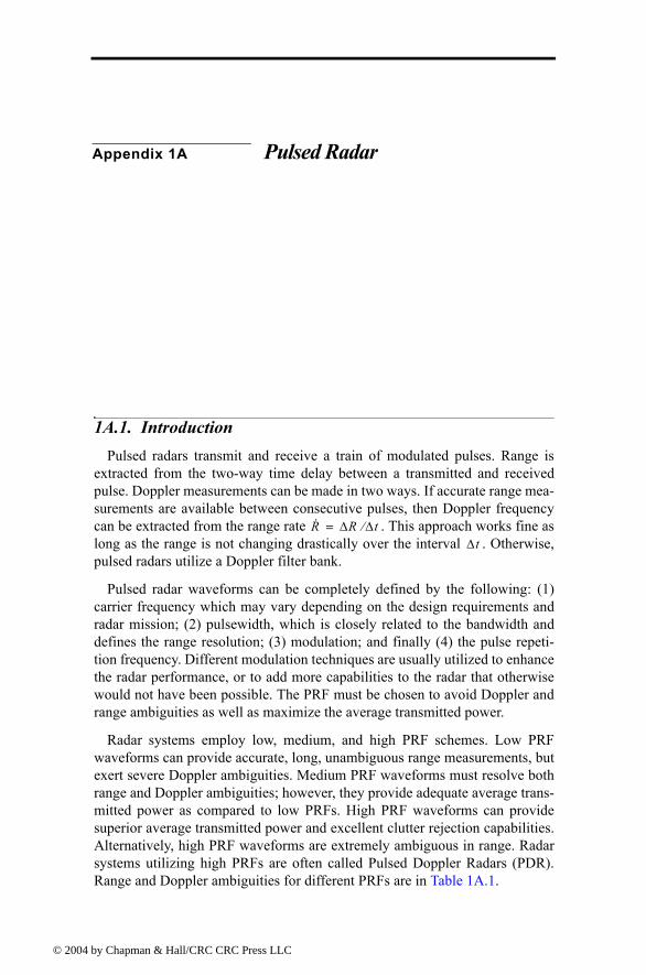
© 200
Appendix 1A Pulsed Radar
1A.1. IntroductionPulsed radars transmit and receive a train of modulated pulses. Range is
extracted from the two-way time delay between a transmitted and received pulse. Doppler measurements can be made in two ways. If accurate range mea-surements are available between consecutive pulses, then Doppler frequency can be extracted from the range rate . This approach works fine as long as the range is not changing drastically over the interval . Otherwise, pulsed radars utilize a Doppler filter bank.
Pulsed radar waveforms can be completely defined by the following: (1) carrier frequency which may vary depending on the design requirements and radar mission; (2) pulsewidth, which is closely related to the bandwidth and defines the range resolution; (3) modulation; and finally (4) the pulse repeti-tion frequency. Different modulation techniques are usually utilized to enhance the radar performance, or to add more capabilities to the radar that otherwise would not have been possible. The PRF must be chosen to avoid Doppler and range ambiguities as well as maximize the average transmitted power.
Radar systems employ low, medium, and high PRF schemes. Low PRF waveforms can provide accurate, long, unambiguous range measurements, but exert severe Doppler ambiguities. Medium PRF waveforms must resolve both range and Doppler ambiguities; however, they provide adequate average trans-mitted power as compared to low PRFs. High PRF waveforms can provide superior average transmitted power and excellent clutter rejection capabilities. Alternatively, high PRF waveforms are extremely ambiguous in range. Radar systems utilizing high PRFs are often called Pulsed Doppler Radars (PDR). Range and Doppler ambiguities for different PRFs are in Table 1A.1.
R· ∆R ∆t⁄=∆t
4 by Chapman & Hall/CRC CRC Press LLC
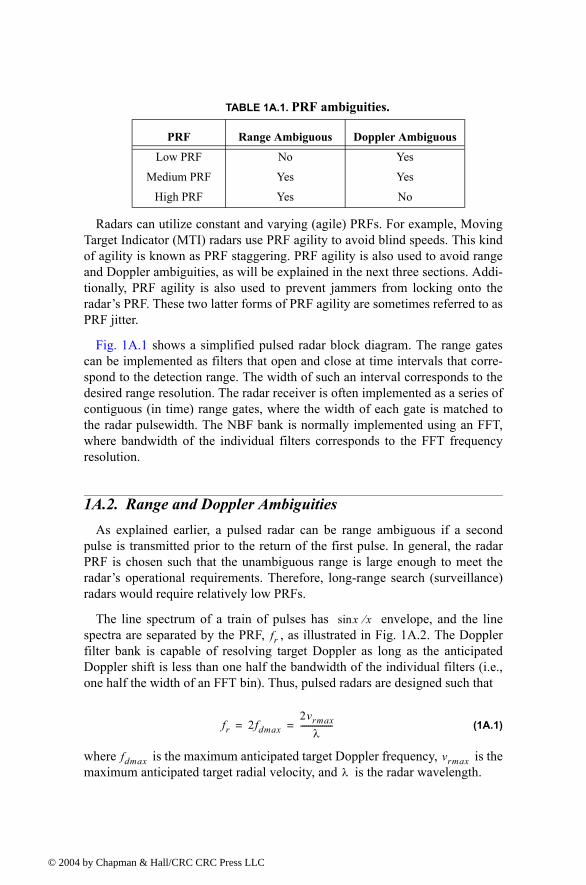
© 200
Radars can utilize constant and varying (agile) PRFs. For example, Moving Target Indicator (MTI) radars use PRF agility to avoid blind speeds. This kind of agility is known as PRF staggering. PRF agility is also used to avoid range and Doppler ambiguities, as will be explained in the next three sections. Addi-tionally, PRF agility is also used to prevent jammers from locking onto the radars PRF. These two latter forms of PRF agility are sometimes referred to as PRF jitter.
Fig. 1A.1 shows a simplified pulsed radar block diagram. The range gates can be implemented as filters that open and close at time intervals that corre-spond to the detection range. The width of such an interval corresponds to the desired range resolution. The radar receiver is often implemented as a series of contiguous (in time) range gates, where the width of each gate is matched to the radar pulsewidth. The NBF bank is normally implemented using an FFT, where bandwidth of the individual filters corresponds to the FFT frequency resolution.
1A.2. Range and Doppler AmbiguitiesAs explained earlier, a pulsed radar can be range ambiguous if a second
pulse is transmitted prior to the return of the first pulse. In general, the radar PRF is chosen such that the unambiguous range is large enough to meet the radars operational requirements. Therefore, long-range search (surveillance) radars would require relatively low PRFs.
The line spectrum of a train of pulses has envelope, and the line spectra are separated by the PRF, , as illustrated in Fig. 1A.2. The Doppler filter bank is capable of resolving target Doppler as long as the anticipated Doppler shift is less than one half the bandwidth of the individual filters (i.e., one half the width of an FFT bin). Thus, pulsed radars are designed such that
(1A.1)
where is the maximum anticipated target Doppler frequency, is the maximum anticipated target radial velocity, and is the radar wavelength.
TABLE 1A.1. PRF ambiguities.
PRF Range Ambiguous Doppler Ambiguous
Low PRF No Yes
Medium PRF Yes Yes
High PRF Yes No
x x⁄sinfr
fr 2fdmax2vrmaxλ
----------------= =
fdmax vrmaxλ
4 by Chapman & Hall/CRC CRC Press LLC
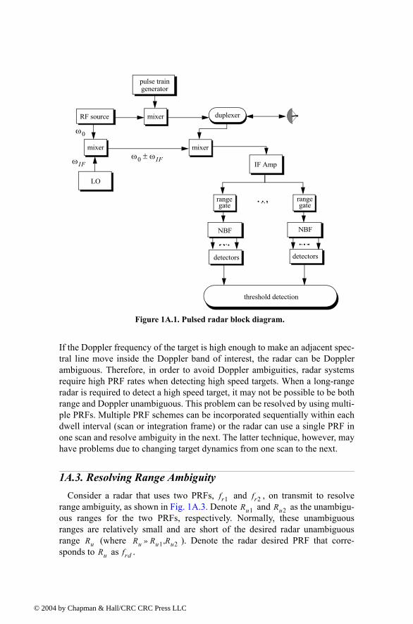
© 200
If the Doppler frequency of the target is high enough to make an adjacent spec-tral line move inside the Doppler band of interest, the radar can be Doppler ambiguous. Therefore, in order to avoid Doppler ambiguities, radar systems require high PRF rates when detecting high speed targets. When a long-range radar is required to detect a high speed target, it may not be possible to be both range and Doppler unambiguous. This problem can be resolved by using multi-ple PRFs. Multiple PRF schemes can be incorporated sequentially within each dwell interval (scan or integration frame) or the radar can use a single PRF in one scan and resolve ambiguity in the next. The latter technique, however, may have problems due to changing target dynamics from one scan to the next.
1A.3. Resolving Range Ambiguity Consider a radar that uses two PRFs, and , on transmit to resolve
range ambiguity, as shown in Fig. 1A.3. Denote and as the unambigu-ous ranges for the two PRFs, respectively. Normally, these unambiguous ranges are relatively small and are short of the desired radar unambiguous range (where ). Denote the radar desired PRF that corre-sponds to as .
RF source
mixer
mixer
mixer
LO
pulse traingenerator
duplexer
IF Amp
rangegate
rangegate
NBF NBF
detectorsdetectors
threshold detection
…
ω0
ω0 ωIF±ωIF
……
…
……
Figure 1A.1. Pulsed radar block diagram.
fr1 fr2Ru1 Ru2
Ru Ru Ru1 Ru2,»Ru frd
4 by Chapman & Hall/CRC CRC Press LLC

© 200
We choose and such that they are relatively prime with respect to one another. One choice is to select and for some integer . Within one period of the desired PRI ( ) the two PRFs
and coincide only at one location, which is the true unambiguous target position. The time delay establishes the desired unambiguous range. The time delays and correspond to the time between the transmit of a pulse on each PRF and receipt of a target return due to the same pulse.
Let be the number of PRF1 intervals between transmit of a pulse and receipt of the true target return. The quantity is similar to except it is for PRF2. It follows that, over the interval to , the only possible results are or . The radar needs only to measure and
. First, consider the case when . In this case,
(1A.2)
for which we get
(1A.3)
where and . It follows that the round trip time to the true target location is
fr
f0-1-2 1 2
fdfd
(a) (b)
Doppler bank
f0-1-2 1 2
f0-1-2 1 2 f0-1-2 1 2
Figure 1A.2. Spectra of transmitted and received waveforms, and Doppler bank. (a) Doppler is resolved. (b) Spectral lines have moved into the next Doppler filter. This results in an ambiguous Dop-pler measurement.
fr1 fr2fr1 Nfrd= fr2 N 1+( )frd=
N Td 1 frd⁄=fr1 fr2
Tdt1 t2
M1M2 M1
0 TdM1 M2 M= = M1 1+ M2= t1
t2 t1 t2<
t1Mfr1------+ t2
Mfr2------+=
Mt2 t1
T1 T2-----------------=
T1 1 fr1⁄= T2 1 fr2⁄=
4 by Chapman & Hall/CRC CRC Press LLC
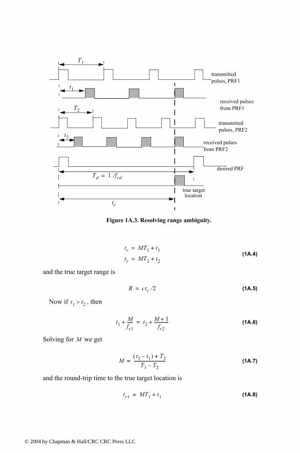
© 200
(1A.4)
and the true target range is
(1A.5)
Now if , then
(1A.6)
Solving for we get
(1A.7)
and the round-trip time to the true target location is
(1A.8)
transmittedpulses, PRF1
transmittedpulses, PRF2
received pulsesfrom PRF1
received pulsesfrom PRF2
desired PRF
true target
Figure 1A.3. Resolving range ambiguity.
location
T1
t1
T2
t2
Td 1 frd⁄=
tr
tr MT1 t1+=
tr MT2 t2+=
R ctr 2⁄=
t1 t2>
t1Mfr1------+ t2
M 1+fr2
--------------+=
M
Mt2 t1( ) T2+
T1 T2-------------------------------=
tr1 MT1 t1+=
4 by Chapman & Hall/CRC CRC Press LLC
© 200
and in this case, the true target range is
(1A.9)
Finally, if , then the target is in the first ambiguity. It follows that
(1A.10)
and
(1A.11)
Since a pulse cannot be received while the following pulse is being transmit-ted, these times correspond to blind ranges. This problem can be resolved by using a third PRF. In this case, once an integer is selected, then in order to guarantee that the three PRFs are relatively prime with respect to one another. In this case, one may choose , , and
.
1A.4. Resolving Doppler AmbiguityThe Doppler ambiguity problem is analogous to that of range ambiguity.
Therefore, the same methodology can be used to resolve Doppler ambiguity. In this case, we measure the Doppler frequencies and instead of and
.
If , then we have
(1A.12)
And if ,
(1A.13)
and the true Doppler is
(1A.14)
Finally, if , then
(1A.15)
Again, blind Doppler can occur, which can be resolved using a third PRF.
Rctr1
2---------=
t1 t2=
tr2 t1 t2= =
R ctr2 2⁄=
N
fr1 N N 1+( )frd= fr2 N N 2+( )frd=fr3 N 1+( ) N 2+( )frd=
fd1 fd2 t1t2
fd1 fd2>
Mfd2 fd1( ) fr2+
fr1 fr2-------------------------------------=
fd1 fd2<
Mfd2 fd1
fr1 fr2-------------------=
fd Mfr1 fd1+=
fd Mfr2 fd2+=
fd1 fd2=
fd fd1 fd2= =
4 by Chapman & Hall/CRC CRC Press LLC
© 200
Example:
A certain radar uses two PRFs to resolve range ambiguities. The desired unambiguous range is . Choose . Compute , ,
, and .
Solution:
First let us compute the desired PRF,
It follows that
.
Example:
Consider a radar with three PRFs; , , and . Assume . Calculate the frequency position of each
PRF for a target whose velocity is . Calculate (Doppler frequency) for another target appearing at , , and for each PRF.
Solution:
The Doppler frequency is
Then by using Eq. (1A.14) where , we can write
We will show here how to compute , and leave the computations of and to the reader. First, if we choose , that means , which
cannot be true since cannot be greater than . Choosing is also
Ru 100Km= N 59= fr1 fr2Ru1 Ru2
frd
frdc
2Ru--------- 3 108×
200 103×----------------------- 1.5KHz= = =
fr1 Nfrd 59( ) 1500( ) 88.5KHz= = =
fr2 N 1+( )frd 59 1+( ) 1500( ) 90KHz= = =
Ru1c
2fr1--------- 3 108×
2 88.5 103××---------------------------------- 1.695Km= = =
Ru2c
2fr2--------- 3 108×
2 90 103××------------------------------ 1.667Km= = =
fr1 15KHz= fr2 18KHz=fr3 21KHz= f0 9GHz=
550m s⁄ fd8KHz 2KHz 17KHz
fd 2vf0c
------- 2 550 9 109×××
3 108×------------------------------------------ 33KHz= = =
nifri fdi+ fd= i 1 2 3, ,=
n1fr1 fd1+ 15n1 fd1+ 33= =
n2fr2 fd2+ 18n2 fd2+ 33= =
n3fr3 fd3+ 21n3 fd3+ 33= =
n1 n2n3 n1 0= fd1 33KHz=
fd1 fr1 n1 1=
4 by Chapman & Hall/CRC CRC Press LLC
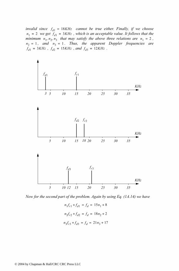
© 200
invalid since cannot be true either. Finally, if we choose we get , which is an acceptable value. It follows that the
minimum that may satisfy the above three relations are , , and . Thus, the apparent Doppler frequencies are
, , and .
Now for the second part of the problem. Again by using Eq. (1A.14) we have
fd1 18KHz=n1 2= fd1 3KHz=
n1 n2 n3, , n1 2=n2 1= n3 1=fd1 3KHz= fd2 15KHz= fd3 12KHz=
KHz
5 10 15 20 25 30 35
fr1fd1
3
KHz
5 10 15 20 25 30 35
fr2fd2
18
KHz
5 10 15 20 25 30 35
fr3fd3
12
n1fr1 fd1+ fd 15n1 8+= =
n2fr2 fd2+ fd 18n2 2+= =
n3fr3 fd3+ fd 21n3 17+= =
4 by Chapman & Hall/CRC CRC Press LLC
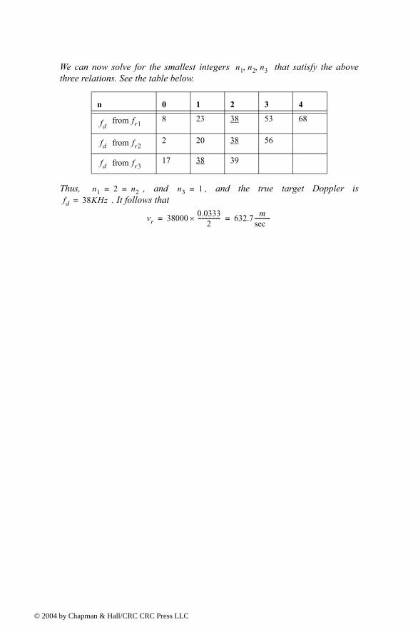
© 200
We can now solve for the smallest integers that satisfy the above three relations. See the table below.
Thus, , and , and the true target Doppler is . It follows that
n 0 1 2 3 4
from 8 23 38 53 68
from 2 20 38 56
from 17 38 39
n1 n2 n3, ,
fdfr1
fd fr2
fd fr3
n1 2 n2= = n3 1=fd 38KHz=
vr 38000 0.03332
----------------× 632.7 msec-----------= =
4 by Chapman & Hall/CRC CRC Press LLC
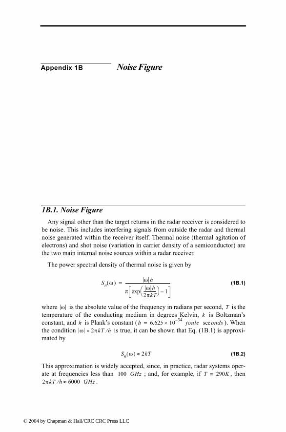
© 200
Appendix 1B Noise Figure
1B.1. Noise FigureAny signal other than the target returns in the radar receiver is considered to
be noise. This includes interfering signals from outside the radar and thermal noise generated within the receiver itself. Thermal noise (thermal agitation of electrons) and shot noise (variation in carrier density of a semiconductor) are the two main internal noise sources within a radar receiver.
The power spectral density of thermal noise is given by
(1B.1)
where is the absolute value of the frequency in radians per second, is the temperature of the conducting medium in degrees Kelvin, is Boltzmans constant, and is Planks constant ( ). When the condition is true, it can be shown that Eq. (1B.1) is approxi-mated by
(1B.2)
This approximation is widely accepted, since, in practice, radar systems oper-ate at frequencies less than ; and, for example, if , then
.
Sn ω( ) ω h
π ω h2πkT------------- exp 1
----------------------------------------------=
ω Tk
h h 6.625 10 34× joule ondssec=ω 2πkT h⁄«
Sn ω( ) 2kT≈
100 GHz T 290K=2πkT h⁄ 6000 GHz≈
4 by Chapman & Hall/CRC CRC Press LLC
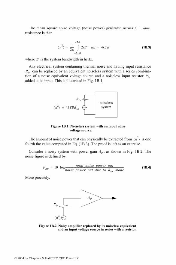
© 200
The mean square noise voltage (noise power) generated across a resistance is then
(1B.3)
where is the system bandwidth in hertz.
Any electrical system containing thermal noise and having input resistance can be replaced by an equivalent noiseless system with a series combina-
tion of a noise equivalent voltage source and a noiseless input resistor added at its input. This is illustrated in Fig. 1B.1.
The amount of noise power that can physically be extracted from is one fourth the value computed in Eq. (1B.3). The proof is left as an exercise.
Consider a noisy system with power gain , as shown in Fig. 1B.2. The noise figure is defined by
(1B.4)
More precisely,
1 ohm
n2⟨ ⟩ 12π------ 2kT ωd
2πB
2πB
∫ 4kTB= =
B
RinRin
noiselesssystemn2⟨ ⟩ 4kTBRin=
Rin
Figure 1B.1. Noiseless system with an input noise voltage source.
n2⟨ ⟩
AP
FdB 10 total noise power outnoise power out due to Rin alone--------------------------------------------------------------------------------------------------log=
Rin
n2⟨ ⟩
AP
Figure 1B.2. Noisy amplifier replaced by its noiseless equivalent and an input voltage source in series with a resistor.
4 by Chapman & Hall/CRC CRC Press LLC
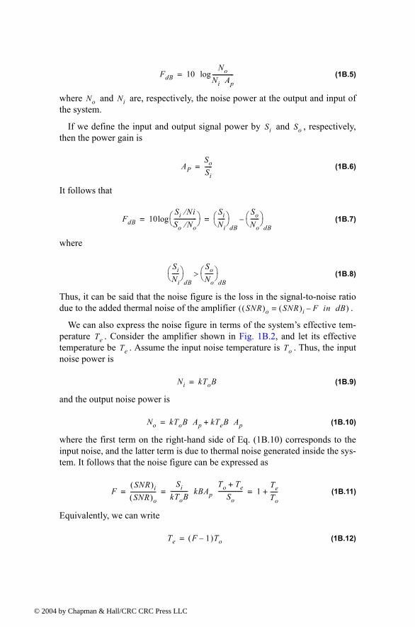
© 200
(1B.5)
where and are, respectively, the noise power at the output and input of the system.
If we define the input and output signal power by and , respectively, then the power gain is
(1B.6)
It follows that
(1B.7)
where
(1B.8)
Thus, it can be said that the noise figure is the loss in the signal-to-noise ratio due to the added thermal noise of the amplifier .
We can also express the noise figure in terms of the systems effective tem-perature . Consider the amplifier shown in Fig. 1B.2, and let its effective temperature be . Assume the input noise temperature is . Thus, the input noise power is
(1B.9)
and the output noise power is
(1B.10)
where the first term on the right-hand side of Eq. (1B.10) corresponds to the input noise, and the latter term is due to thermal noise generated inside the sys-tem. It follows that the noise figure can be expressed as
(1B.11)
Equivalently, we can write
(1B.12)
FdB 10No
Ni Ap---------------log=
No Ni
Si So
APSoSi-----=
FdB 10Si Ni⁄So No⁄---------------- log
SiNi-----
dB
SoNo------
dB= =
SiNi-----
dB
SoNo------
dB>
SNR( )o SNR( )i F in dB=( )
TeTe To
Ni kToB=
No kToB Ap kTeB Ap+=
FSNR( )iSNR( )o
------------------Si
kToB------------ kBAp
To Te+
So----------------- 1
TeTo-----+= = =
Te F 1( )To=
4 by Chapman & Hall/CRC CRC Press LLC
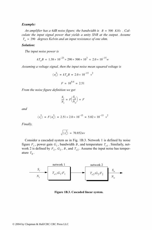
© 200
Example:
An amplifier has a 4dB noise figure; the bandwidth is . Cal-culate the input signal power that yields a unity SNR at the output. Assume
degrees Kelvin and an input resistance of one ohm.
Solution:
The input noise power is
Assuming a voltage signal, then the input noise mean squared voltage is
From the noise figure definition we get
and
Finally,
Consider a cascaded system as in Fig. 1B.3. Network 1 is defined by noise figure , power gain , bandwidth , and temperature . Similarly, net-work 2 is defined by , , , and . Assume the input noise has temper-ature .
B 500 KHz=
To 290=
kToB 1.38 10 23× 290 500 103××× 2.0 10 15× w= =
ni2⟨ ⟩ kToB 2.0 10 15× v2
= =
F 100.4 2.51= =
SiNi----- F
SoNo------ F= =
si2⟨ ⟩ F ni
2⟨ ⟩ 2.51 2.0 10 15×× 5.02 10 15× v2= = =
si2⟨ ⟩ 70.852nv=
F1 G1 B Te1F2 G2 B Te2
T0
network 2
Te2 G2; F2;Te1 G1 F1;;Si
Ni No
So
Figure 1B.3. Cascaded linear system.
network 1
4 by Chapman & Hall/CRC CRC Press LLC
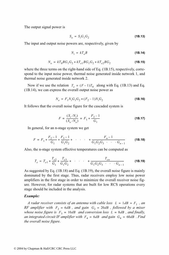
© 200
The output signal power is
(1B.13)
The input and output noise powers are, respectively, given by
(1B.14)
(1B.15)
where the three terms on the right-hand side of Eq. (1B.15), respectively, corre-spond to the input noise power, thermal noise generated inside network 1, and thermal noise generated inside network 2.
Now if we use the relation along with Eq. (1B.13) and Eq. (1B.14), we can express the overall output noise power as
(1B.16)
It follows that the overall noise figure for the cascaded system is
(1B.17)
In general, for an n-stage system we get
(1B.18)
Also, the n-stage system effective temperatures can be computed as
(1B.19)
As suggested by Eq. (1B.18) and Eq. (1B.19), the overall noise figure is mainly dominated by the first stage. Thus, radar receivers employ low noise power amplifiers in the first stage in order to minimize the overall receiver noise fig-ure. However, for radar systems that are built for low RCS operations every stage should be included in the analysis.
Example:
A radar receiver consists of an antenna with cable loss , an RF amplifier with , and gain , followed by a mixer whose noise figure is and conversion loss , and finally, an integrated circuit IF amplifier with and gain . Find the overall noise figure.
So SiG1G2=
Ni kToB=
No kT0BG1G2 kTe1BG1G2 kTe2BG2+ +=
Te F 1( )T0=
No F1NiG1G2 F2 1( )NiG2+=
FSi Ni⁄( )So No⁄( )
-------------------- F1F2 1
G1---------------+= =
F F1F2 1
G1---------------
F3 1
G1G2--------------- ⋅ ⋅ ⋅
Fn 1
G1G2G3 Gn 1⋅ ⋅ ⋅----------------------------------------------------------+ + + +=
Te Te1Te2G1--------
Te3G1G2--------------
TenG1G2G3 Gn 1⋅ ⋅ ⋅----------------------------------------------------------+⋅ ⋅ ⋅+ + +=
L 1dB F1= =F2 6dB= G2 20dB=
F3 10dB= L 8dB=F4 6dB= G4 60dB=
4 by Chapman & Hall/CRC CRC Press LLC
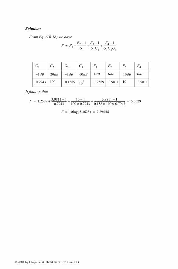
© 200
Solution:
From Eq. (1B.18) we have
It follows that
F F1F2 1
G1---------------
F3 1
G1G2---------------
F4 1
G1G2G3---------------------+ + +=
G1 G2 G3 G4 F1 F2 F3 F4
1dB 20dB 8dB 60dB 1dB 6dB 10dB 6dB
0.7943 100 0.1585 106 1.2589 3.9811 10 3.9811
F 1.2589 3.9811 10.7943
------------------------- 10 1100 0.7943×------------------------------- 3.9811 1
0.158 100× 0.7943×---------------------------------------------------+ + + 5.3629= =
F 10 5.3628( )log 7.294dB= =
4 by Chapman & Hall/CRC CRC Press LLC
© 200
Chapter 2 Radar Detection
2.1. Detection in the Presence of NoiseA simplified block diagram of a radar receiver that employs an envelope
detector followed by a threshold decision is shown in Fig. 2.1. The input signal to the receiver is composed of the radar echo signal and additive zero mean white Gaussian noise , with variance . The input noise is assumed to be spatially incoherent and uncorrelated with the signal.
The output of the bandpass IF filter is the signal , which can be written as
(2.1)
where is the radar operating frequency, is the envelope of , the phase is , and the subscripts , respectively,
refer to the in-phase and quadrature components.
A target is detected when exceeds the threshold value , where the decision hypotheses are
s t( )n t( ) ψ2
v t( )
v t( ) vI t( ) ω0tcos vQ t( ) ω0tsin+ r t( ) ω0t ϕ t( )( )cos= =
vI t( ) r t( ) ϕ t( )cos=
vQ t( ) r t( ) ϕ t( )sin=
ω0 2πf0= r t( )v t( ) ϕ t( ) vQ vI⁄( )atan= I Q,
r t( ) VT
s t( ) n t( )+ VT> Detectionn t( ) VT> False alarm
4 by Chapman & Hall/CRC CRC Press LLC
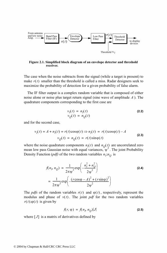
© 200
The case when the noise subtracts from the signal (while a target is present) to make smaller than the threshold is called a miss. Radar designers seek to maximize the probability of detection for a given probability of false alarm.
The IF filter output is a complex random variable that is composed of either noise alone or noise plus target return signal (sine wave of amplitude ). The quadrature components corresponding to the first case are
(2.2)
and for the second case,
(2.3)
where the noise quadrature components and are uncorrelated zero mean low pass Gaussian noise with equal variances, . The joint Probability Density Function (pdf) of the two random variables is
(2.4)
The pdfs of the random variables and , respectively, represent the modulus and phase of . The joint pdf for the two random variables
is given by
(2.5)
where is a matrix of derivatives defined by
From antennaand low noise Band Pass
Filter (IF)EnvelopeDetector
Low PassFilter
Threshold VT
ThresholdDetector to display
devicesv t( )
r t( )Amp.
Figure 2.1. Simplified block diagram of an envelope detector and threshold receiver.
r t( )
A
vI t( ) nI t( )vQ t( ) nQ t( )
==
vI t( ) A nI t( )+ r t( ) ϕ t( )cos= = nI t( )⇒ r t( ) ϕ t( )cos A=
vQ t( ) nQ t( ) r t( ) ϕ t( )sin= =
nI t( ) nQ t( )ψ2
nI nQ;
f nI nQ,( ) 12πψ2------------- nI
2 nQ2+
2ψ2-----------------
exp
12πψ2------------- r ϕcos A( )2 r ϕsin( )2+
2ψ2-----------------------------------------------------------
exp
=
=
r t( ) ϕ t( )v t( )
r t( ) ϕ t( );
f r ϕ,( ) f nI nQ,( ) J=
J[ ]
4 by Chapman & Hall/CRC CRC Press LLC
© 200
(2.6)
The determinant of the matrix of derivatives is called the Jacobian, and in this case it is equal to
(2.7)
Substituting Eqs. (2.4) and (2.7) into Eq. (2.5) and collecting terms yield
(2.8)
The pdf for alone is obtained by integrating Eq. (2.8) over
(2.9)
where the integral inside Eq. (2.9) is known as the modified Bessel function of zero order,
(2.10)
Thus,
(2.11)
which is the Rician probability density function. If (noise alone), then Eq. (2.11) becomes the Rayleigh probability density function
(2.12)
Also, when is very large, Eq. (2.11) becomes a Gaussian probability density function of mean and variance :
J[ ] r∂∂nI
ϕ∂∂nI
r∂∂nQ
ϕ∂∂nQ
ϕcos r ϕsin
ϕsin r ϕcos= =
J r t( )=
f r ϕ,( ) r2πψ2------------- r2 A2+
2ψ2-----------------
rA ϕcos
ψ2------------------- expexp=
r ϕ
f r( ) f r ϕ,( ) ϕd
0
2π
∫ rψ2------ r2 A2+
2ψ2-----------------
1
2π------ rA ϕcos
ψ2------------------- exp ϕd
0
2π
∫exp= =
I0 β( ) 12π------ eβ θcos θd
0
2π
∫=
f r( ) rψ2------I0
rAψ2------ r2 A2+
2ψ2-----------------
exp=
A ψ2⁄ 0=
f r( ) rψ2------ r2
2ψ2---------
exp=
A ψ2⁄( )A ψ2
4 by Chapman & Hall/CRC CRC Press LLC
© 200
(2.13)
Fig. 2.2 shows plots for the Rayleigh and Gaussian densities. For this purpose, use MATLAB program fig2_2.m given in Listing 2.1 in Section 2.11. This program uses MATLAB functions normpdf.m and raylpdf.m. Both func-tions are part of the MATLAB Statistics toolbox. Their associated syntax is as follows
normpdf(x,mu,sigma)
raylpdf(x,sigma)
x is the variable, mu is the mean, and sigma is the standard deviation.
The density function for the random variable is obtained from
(2.14)
While the detailed derivation is left as an exercise, the result of Eq. (2.14) is
(2.15)
f r( ) 1
2πψ2----------------- r A( )2
2ψ2-------------------
exp≈
Figure 2.2. Gaussian and Rayleigh probability densities.
ϕ
f ϕ( ) f r ϕ,( ) rd
0
r
∫=
f ϕ( ) 12π------ A2
2ψ2---------
exp A ϕcos
2πψ2----------------- A ϕsin( )2
2ψ2--------------------------
exp F A ϕcosψ
---------------- +=
4 by Chapman & Hall/CRC CRC Press LLC
© 200
where
(2.16)
The function can be found tabulated in most mathematical formula refer-ence books. Note that for the case of noise alone ( ), Eq. (2.15) collapses to a uniform pdf over the interval .
One excellent approximation for the function is
(2.17)
and for negative values of
(2.18)
MATLAB Function que_func.m
The function que_func.m computes using Eqs. (2.17) and (2.18) and is given in Listing 2.2 in Section 2.11. The syntax is as follows:
fofx = que_func (x)
2.2. Probability of False AlarmThe probability of false alarm is defined as the probability that a sample of the signal will exceed the threshold voltage when noise alone is
present in the radar,
(2.19a)
(2.19b)
Fig. 2.3 shows a plot of the normalized threshold versus the probability of false alarm. It is evident from this figure that is very sensitive to small changes in the threshold value. This figure can be reproduced using MATLAB program fig2_3.m given in Listing 2.3 in Section 2.11.
The false alarm time is related to the probability of false alarm by
F x( ) 12π
---------- e ζ 2 2⁄ ξd
∞
x
∫=
F x( )A 0=
0 2π,
F x( )
F x( ) 1 1
0.661x 0.339 x2 5.51++-------------------------------------------------------------- 1
2π----------e x2 2⁄= x 0≥
x
F x( ) 1 F x( )=
F x( )
PfaR r t( ) VT
Pfarψ2------ r2
2ψ2---------
exp rd
VT
∞
∫VT
2
2ψ2---------
exp= =
VT 2ψ2 1Pfa------- ln=
Pfa
Tfa
4 by Chapman & Hall/CRC CRC Press LLC
© 200
(2.20)
where represents the radar integration time, or the average time that the output of the envelope detector will pass the threshold voltage. Since the radar operating bandwidth is the inverse of , then by substituting Eq. (2.19) into Eq. (2.20) we can write as
(2.21)
Minimizing means increasing the threshold value, and as a result the radar maximum detection range is decreased. Therefore, the choice of an acceptable value for becomes a compromise depending on the radar mode of opera-tion.
Fehlner1 defines the false alarm number as
(2.22)
1. Fehlner, L. F., Marcums and Swerlings Data on Target Detection by a Pulsed Radar, Johns Hopkins University, Applied Physics Lab. Rpt. # TG451, July 2, 1962, and Rpt. # TG451A, September 1964.
VT
2ψ2--------------
Figure 2.3. Normalized detection threshold versus probability of false alarm.
1 Pfa⁄( )log
Tfa tint Pfa⁄=
tint
B tintTfa
Tfa1B---
VT2
2ψ2---------
exp=
Tfa
Tfa
nfa2( )ln
1 Pfa( )ln--------------------------=
2( )lnPfa
-------------≈
4 by Chapman & Hall/CRC CRC Press LLC
© 200
Other slightly different definitions for the false alarm number exist in the liter-ature, causing a source of confusion for many non-expert readers. Other than the definition in Eq. (2.22), the most commonly used definition for the false alarm number is the one introduced by Marcum (1960). Marcum defines the false alarm number as the reciprocal of . In this text, the definition given in Eq. (2.22) is always assumed. Hence, a clear distinction is made between Mar-cums definition of the false alarm number and the definition in Eq. (2.22).
2.3. Probability of DetectionThe probability of detection is the probability that a sample of
will exceed the threshold voltage in the case of noise plus signal,
(2.23)
If we assume that the radar signal is a sine waveform with amplitude , then its power is . Now, by using (single-pulse SNR) and
, then Eq. (2.23) can be rewritten as
(2.24)
(2.25)
is called Marcums Q-function. When is small and is relatively large so that the threshold is also large, Eq. (2.24) can be approximated by
(2.26)
where is given by Eq. (2.16). Many approximations for computing Eq. (2.24) can be found throughout the literature. One very accurate approximation presented by North (see bibliography) is given by
(2.27)
where the complementary error function is
Pfa
PD R r t( )
PDrψ2------ I0
rAψ2------ r2 A2+
2ψ2-----------------
exp rd
VT
∞
∫=
AA2 2⁄ SNR A2 2ψ2⁄=
VT2 2ψ2⁄( ) 1 Pfa⁄( )ln=
PDrψ2------I0
rAψ2------ r2 A2+
2ψ2-----------------
exp rd
2ψ2 1 pfa⁄( )ln
∞
∫
Q A2
ψ2------ 2 1
Pfa------- ln,
= =
Q α β,[ ] ζI0 αζ( )e ζ2 α2+( ) 2⁄ ζd
β
∞
∫=
Q Pfa PD
PD F Aψ---- 2 1
Pfa------- ln
≈
F x( )
PD 0.5 erfc Pfaln SNR 0.5+( )×≈
4 by Chapman & Hall/CRC CRC Press LLC
© 200
(2.28)
MATLAB Function marcumsq.m
The integral given in Eq. (2.24) is complicated and can be computed using numerical integration techniques. Parl1 developed an excellent algorithm to numerically compute this integral. It is summarized as follows:
(2.29)
(2.30)
(2.31)
(2.32)
(2.33)
(2.34)
, , and . The recursive Eqs. (2.30) through (2.32) are computed continuously until for values of . The accuracy of the algorithm is enhanced as the value of is increased. The MATLAB func-tion marcumsq.m given in Listing 2.4 in Section 2.11 implements Parls algorithm to calculate the probability of detection defined in Eq. (2.24). The syntax is as follows:
Pd = marcumsq (alpha, beta)where alpha and beta are from Eq. (2.25). Fig. 2.4 shows plots of the probabil-ity of detection, , versus the single pulse SNR, with the as a parameter. This figure can be reproduced using the MATLAB program prob_snr1.mgiven in Listing 2.5 in Section 2.11.
1. Parl, S., A New Method of Calculating the Generalized Q Function, IEEE Trans. Information Theory, Vol. IT-26, No. 1, January 1980, pp. 121-124.
erfc z( ) 1 2π
------- e ν2 νd
0
z
∫=
Q a b,[ ]
αn
2βn-------- a b( )2
2------------------- exp a b<
1αn
2βn-------- a b( )2
2------------------- exp a b≥
=
αn dn2nab------αn 1 αn 2++=
βn 1 2nab------βn 1 βn 2+ +=
dn 1+ dnd1=
α01 a b<0 a b≥
=
d1a b⁄ a b<b a⁄ a b≥
=
α 1 0.0= β0 0.5= β 1 0=βn 10p> p 3≥
p
PD Pfa
4 by Chapman & Hall/CRC CRC Press LLC
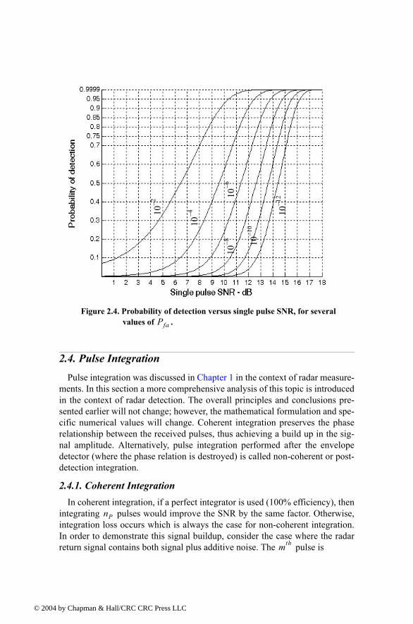
© 200
2.4. Pulse IntegrationPulse integration was discussed in Chapter 1 in the context of radar measure-
ments. In this section a more comprehensive analysis of this topic is introduced in the context of radar detection. The overall principles and conclusions pre-sented earlier will not change; however, the mathematical formulation and spe-cific numerical values will change. Coherent integration preserves the phase relationship between the received pulses, thus achieving a build up in the sig-nal amplitude. Alternatively, pulse integration performed after the envelope detector (where the phase relation is destroyed) is called non-coherent or post-detection integration.
2.4.1. Coherent IntegrationIn coherent integration, if a perfect integrator is used (100% efficiency), then
integrating pulses would improve the SNR by the same factor. Otherwise, integration loss occurs which is always the case for non-coherent integration. In order to demonstrate this signal buildup, consider the case where the radar return signal contains both signal plus additive noise. The pulse is
Figure 2.4. Probability of detection versus single pulse SNR, for several values of .Pfa
102
106
104 10
12
108 10
10
nP
mth
4 by Chapman & Hall/CRC CRC Press LLC
© 200
(2.35)
where is the radar return of interest and is white uncorrelated addi-tive noise signal. Coherent integration of pulses yields
(2.36)
The total noise power in is equal to the variance. More precisely,
(2.37)
where is the expected value operator. It follows that
(2.38)
where is the single pulse noise power and is equal to zero for and unity for . Observation of Eqs. (2.36) and (2.38) shows that the desired signal power after coherent integration is unchanged, while the noise power is reduced by the factor . Thus, the SNR after coherent integration is improved by .
Denote the single pulse SNR required to produce a given probability of detection as . Also, denote as the SNR required to produce the same probability of detection when pulses are integrated. It follows that
(2.39)
The requirements of knowing the exact phase of each transmitted pulse as well as maintaining coherency during propagation is very costly and challenging to achieve. Thus, radar systems would not utilize coherent integration during search mode, since target micro-dynamics may not be available.
2.4.2. Non-Coherent Integration
Non-coherent integration is often implemented after the envelope detector, also known as the quadratic detector. A block diagram of radar receiver utiliz-ing a square law detector and non-coherent integration is illustrated in Fig. 2.5. In practice, the square law detector is normally used as an approximation to the optimum receiver.
ym t( ) s t( ) nm t( )+=
s t( ) nm t( )nP
z t( ) 1nP----- ym t( )
m 1=
nP
∑ 1nP----- s t( ) nm t( )+[ ]
m 1=
nP
∑ s t( ) 1nP-----nm t( )
m 1=
nP
∑+= = =
z t( )
ψnz2 E 1
nP-----nm t( )
m 1=
nP
∑ 1
nP-----nl t( )
l 1=
nP
∑ ∗
=
E[ ]
ψnz2 1
nP2
----- E nm t( )nl∗ t( )[ ]
m l, 1=
nP
∑ 1nP
2----- ψny
2 δml
m l, 1=
nP
∑ 1nP-----ψny
2= = =
ψny2 δml m l≠
m l=
1 nP⁄nP
SNR( )1 SNR( )nPnP
SNR( )nP
1nP----- SNR( )1=
4 by Chapman & Hall/CRC CRC Press LLC
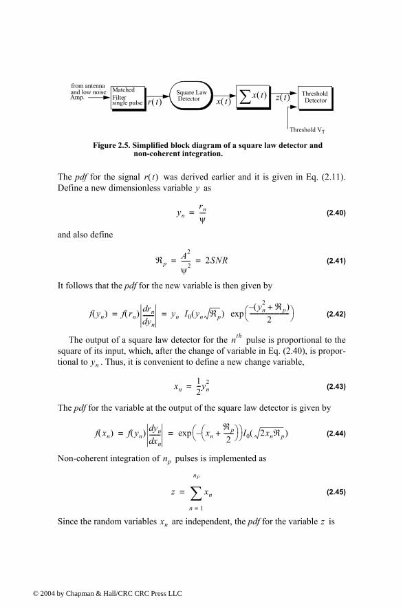
© 200
The pdf for the signal was derived earlier and it is given in Eq. (2.11). Define a new dimensionless variable as
(2.40)
and also define
(2.41)
It follows that the pdf for the new variable is then given by
(2.42)
The output of a square law detector for the pulse is proportional to the square of its input, which, after the change of variable in Eq. (2.40), is propor-tional to . Thus, it is convenient to define a new change variable,
(2.43)
The pdf for the variable at the output of the square law detector is given by
(2.44)
Non-coherent integration of pulses is implemented as
(2.45)
Since the random variables are independent, the pdf for the variable is
from antennaand low noise Matched
FilterSquare Law Detector
Threshold VT
ThresholdDetectorr t( )
x t( )∑Amp.
Figure 2.5. Simplified block diagram of a square law detector and non-coherent integration.
x t( ) z t( )single pulse
r t( )y
ynrn
ψ----=
ℜpA2
ψ2------ 2SNR= =
f yn( ) f rn( ) rndynd
------- yn I0 yn ℜp( )yn
2 ℜp+( )
2-------------------------- exp= =
nth
yn
xn12---yn
2=
f xn( ) f yn( ) yndxnd
------- xnℜp
2-------+
exp I0 2xnℜp( )= =
np
z xn
n 1=
nP
∑=
xn z
4 by Chapman & Hall/CRC CRC Press LLC
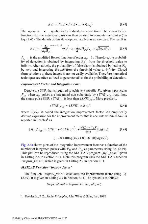
© 200
(2.46)
The operator symbolically indicates convolution. The characteristic functions for the individual pdfs can then be used to compute the joint pdf in Eq. (2.46). The details of this development are left as an exercise. The result is
(2.47)
is the modified Bessel function of order . Therefore, the probabil-ity of detection is obtained by integrating from the threshold value to infinity. Alternatively, the probability of false alarm is obtained by letting be zero and integrating the pdf from the threshold value to infinity. Closed form solutions to these integrals are not easily available. Therefore, numerical techniques are often utilized to generate tables for the probability of detection.
Improvement Factor and Integration Loss
Denote the SNR that is required to achieve a specific given a particular when pulses are integrated non-coherently by . And thus,
the single pulse SNR, , is less than . More precisely,
(2.48)
where is called the integration improvement factor. An empirically derived expression for the improvement factor that is accurate within is reported in Peebles1 as
(2.49)
Fig. 2.6a shows plots of the integration improvement factor as a function of the number of integrated pulses with and as parameters, using Eq. (2.49). This plot can be reproduced using the MATLAB program fig2_6a.m given in Listing 2.6 in Section 2.11. Note this program uses the MATLAB function improv_fac.m, which is given in Listing 2.7 in Section 2.11.
MATLAB Function improv_fac.m
The function improv_fac.m calculates the improvement factor using Eq. (2.49). It is given in Listing 2.7 in Section 2.11. The syntax is as follows:
[impr_of_np] = improv_fac (np, pfa, pd)
1. Peebles Jr., P. Z., Radar Principles, John Wiley & Sons, Inc., 1998.
f z( ) f x1( ) f x2( ) … f xnp( )•••=
•
f z( ) 2znPℜp-------------
nP 1( ) 2⁄z
12---nPℜp
exp InP 1 2nPzℜp( )=
InP 1 nP 1f z( )
ℜp
PDPfa nP SNR( )NCI
SNR( )1 SNR( )NCI
SNR( )NCI SNR( )1 I nP( )×=
I nP( )0.8dB
I nP( )[ ]dB 6.79 1 0.235PD+( ) 11 Pfa⁄( )log
46.6---------------------------+
nP( )
1 0.140 nP( )log 0.018310 nPlog( )2+( )
log=
PD Pfa
4 by Chapman & Hall/CRC CRC Press LLC
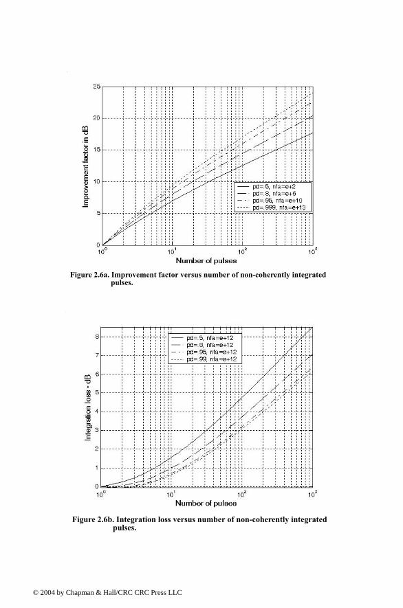
© 200
Figure 2.6a. Improvement factor versus number of non-coherently integrated pulses.
Figure 2.6b. Integration loss versus number of non-coherently integrated pulses.
4 by Chapman & Hall/CRC CRC Press LLC
© 200
where
The integration loss is defined as
(2.50)
Figure 2.6b shows a plot of the integration loss versus . This figure can be reproduced using MATLAB program fig2_6b.m given in Listing 2.8 in Sec-tion 2.11. It follows that, when non-coherent integration is utilized, the corre-sponding SNR required to achieve a certain given a specific is now given by
(2.51)
which is very similar to Eq. (1.86) derived in Chapter 1.
2.4.3. Mini Design Case Study 2.1
An L-band radar has the following specifications: operating frequency , operating bandwidth , noise figure ,
system losses , time of false alarm , detection
range , the minimum required SNR is , antenna
gain , and target RCS . (a) Determine the PRF , the
pulsewidth , the peak power , the probability of false alarm , the corre-
sponding , and the minimum detectable signal level . (b) How can you reduce the transmitter power to achieve the same performance when 10 pulses are integrated non-coherently? (c) If the radar operates at a shorter range in the single pulse mode, find the new probability of detection when the range decreases to .
A Solution
Assume that the maximum detection corresponds to the unambiguous range. From that the PRF is computed as
Symbol Description Units Status
np number of integrated pulses none input
pfa probability of false alarm none input
pd probability of detection none input
impr_of_np improvement factor output dB
LNCI nP I nP( )⁄=
nP
PD Pfa
SNR( )NCI nP SNR( )× 1( ) LNCI⁄=
f0 1.5GHz= B 2MHz= F 8dB=
L 4dB= Tfa 12 minutes=
R 12Km= SNR 13.85dB=
G 5000= σ 1m2= fr
τ Pt Pfa
PD Smin
9Km
4 by Chapman & Hall/CRC CRC Press LLC
© 200
The pulsewidth is proportional to the inverse of the bandwidth,
The probability of false alarm is
It follows that by using MATLAB functionmarcumsq.mthe probability of detection is calculated from
with the following syntax
marcumsq(alpha, beta)
where
Remember that . Thus, the detection probability is
Using the radar equation one can calculate the radar peak power. More pre-cisely,
And the minimum detectable signal is
frc
2Ru--------- 3 108×
2 12000×------------------------ 12.5KHz= = =
τ 1B--- 1
2 106×----------------- 0.5µs= = =
Pfa1
BTfa----------- 1
2 106× 12 60××------------------------------------------ 6.94 10 10×= = =
Q A2
ψ2------ 2 1
Pfa------- ln,
alpha 2 1013.85 10⁄× 6.9665= =
beta 2 16.94 10 10×----------------------------- ln 6.494= =
A2 ψ2⁄( ) 2SNR=
PD marcumsq 6.9665 6.944,( ) 0.508= =
Pt SNR4π( )3R4kT0BFL
G2λ2σ----------------------------------------= ⇒
Pt 101.385 4π( )3 120004 1.38 10 23×× 290× 2 106×× 6.309× 2.511××
50002 0.22× 1×--------------------------------------------------------------------------------------------------------------------------------------------------------
126.61Watts
=
=
4 by Chapman & Hall/CRC CRC Press LLC
© 200
When 10 pulses are integrated non-coherently, the corresponding improvement factor is calculated from the MATLAB function improv_fac.m using the fol-lowing syntax
improv_fac (10,1e-11,0.5)
which yields . Consequently, by keeping the probability of detection the same (with and without integration) the SNR can be reduced by a factor of almost 6 dB (13.85 - 7.78). The integration loss associated with a 10-pulse non-coherent integration is calculated from Eq. (2.50) as
Thus the net single pulse SNR with 10-pulse non-coherent integration is
.
Finally, the improvement in the SNR due to decreasing the detection range to 9 Km is
.
2.5. Detection of Fluctuating Targets So far the probability of detection calculations assumed a constant target
cross section (non-fluctuating target). This work was first analyzed by Mar-cum.1 Swerling2 extended Marcums work to four distinct cases that account for variations in the target cross section. These cases have come to be known as Swerling models. They are: Swerling I, Swerling II, Swerling III, and Swerling IV. The constant RCS case analyzed by Marcum is widely known as Swerling 0 or equivalently Swerling V. Target fluctuation lowers the probability of detection, or equivalently reduces the SNR.
1. Marcum, J. I., A Statistical Theory of Target Detection by Pulsed Radar, IRE Trans-actions on Information Theory. Vol IT-6, pp 59-267. April 1960.
2. Swerling, P., Probability of Detection for Fluctuating Targets, IRE Transactions on Information Theory. Vol IT-6, pp 269-308. April 1960.
SminPtG
2λ2σ
4π( )3R4L----------------------- 126.61 50002 0.22× 1××
4π( )3 120004 2.511××-------------------------------------------------------------- 1.2254 10 12× Volts= = =
I 10( ) 6= 7.78dB⇒
LNCInP
I 10( )------------- 10
6------ 1.67 2.2dB⇒= = =
SNR( )NCI 13.85 7.78 2.2+ 8.27dB= =
SNR( )9Km 10 120009000
--------------- log
413.85+ 18.85dB= =
4 by Chapman & Hall/CRC CRC Press LLC
© 200
Swerling I targets have constant amplitude over one antenna scan; however, a Swerling I target amplitude varies independently from scan to scan according to a Chi-square probability density function with two degrees of freedom. The amplitude of Swerling II targets fluctuates independently from pulse to pulse according to a Chi-square probability density function with two degrees of freedom. Target fluctuation associated with a Swerling III model is similar to Swerling I, except in this case the target power fluctuates independently from pulse to pulse according to a Chi-square probability density function with four degrees of freedom. Finally, the fluctuation of Swerling IV targets is from pulse to pulse according to a Chi-square probability density function with four degrees of freedom. Swerling showed that the statistics associated with Swer-ling I and II models apply to targets consisting of many small scatterers of comparable RCS values, while the statistics associated with Swerling III and IV models apply to targets consisting of one large RCS scatterer and many small equal RCS scatterers. Non-coherent integration can be applied to all four Swerling models; however, coherent integration cannot be used when the tar-get fluctuation is either Swerling II or Swerling IV. This is because the target amplitude decorrelates from pulse to pulse (fast fluctuation) for Swerling II and IV models, and thus phase coherency cannot be maintained.
The Chi-square pdf with degrees of freedom can be written as
(2.52)
where is the average RCS value. Using this equation, the pdf associated with Swerling I and II targets can be obtained by letting , which yields a Rayleigh pdf. More precisely,
(2.53)
Letting yields the pdf for Swerling III and IV type targets,
(2.54)
The probability of detection for a fluctuating target is computed in a similar fashion to Eq. (2.23), except in this case is replaced by the conditional pdf
. Performing the analysis for the general case (i.e., using Eq. (2.47)) yields
(2.55)
2N
f σ( ) NN 1( )! σ
--------------------------- Nσσ
------- N 1 Nσ
σ-------
exp=
σN 1=
f σ( ) 1σ--- σ
σ---
exp= σ 0≥
N 2=
f σ( ) 4σσ
2------ 2σ
σ------
exp= σ 0≥
f r( )f r σ⁄( )
f z σ⁄( ) 2znPσ
2 ψ2⁄---------------------- nP 1( ) 2⁄
z12---nP
σ2
ψ2------
exp InP 1 2nPzσ2
ψ2------
=
4 by Chapman & Hall/CRC CRC Press LLC
© 200
To obtain use the relations
(2.56)
(2.57)
Finally, using Eq. (2.56) in Eq. (2.57) produces
(2.58)
where is defined in Eq. (2.55) and is in either Eq. (2.53) or (2.54). The probability of detection is obtained by integrating the pdf derived from Eq. (2.58) from the threshold value to infinity. Performing the integration in Eq. (2.58) leads to the incomplete Gamma function.
2.5.1. Threshold Selection
When only a single pulse is used, the detection threshold is related to the probability of false alarm as defined in Eq. (2.19). DiFranco and Rubin1
derived a general form relating the threshold and for any number of pulses when non-coherent integration is used. It is
(2.59)
where is used to denote the incomplete Gamma function. It is given by
(2.60)
Note that the limiting values for the incomplete Gamma function are
(2.61)
For our purposes, the incomplete Gamma function can be approximated by
(2.62)
1. DiFranco, J. V. and Rubin, W. L., Radar Detection, Artech House, 1980.
f z( )
f z σ,( ) f z σ⁄( )f σ( )=
f z( ) f z σ,( ) σd∫=
f z( ) f z σ⁄( )f σ( ) σd∫=
f z σ⁄( ) f σ( )
VTPfa
Pfa
Pfa 1 ΓIVT
nP
---------- nP 1,
=
ΓI
ΓIVT
nP
---------- nP 1, e γ γ
nP 1( ) 1
nP 1( ) 1( )!----------------------------------- γd
0
VT nP⁄
∫=
ΓI 0 N,( ) 0= ΓI ∞ N,( ) 1=
ΓIVT
nP
---------- nP 1,
1VT
nP 1e
VT
nP 1( )!--------------------------- 1
nP 1
VT--------------
nP 1( ) nP 2( )
VT2
---------------------------------------
…nP 1( )!
VTnP 1
---------------------
+ + +
+
=
4 by Chapman & Hall/CRC CRC Press LLC
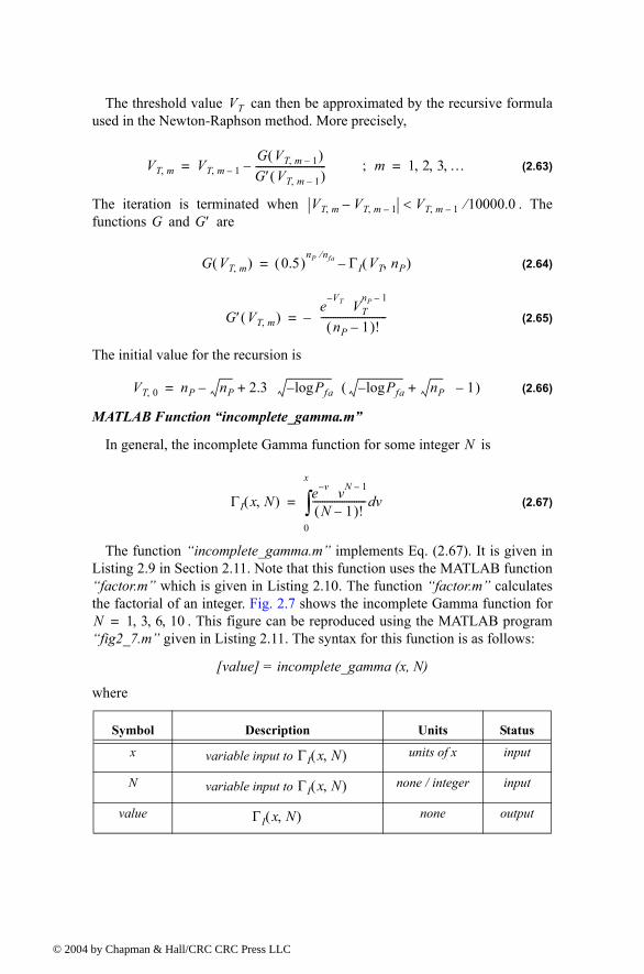
© 200
The threshold value can then be approximated by the recursive formula used in the Newton-Raphson method. More precisely,
(2.63)
The iteration is terminated when . The functions and are
(2.64)
(2.65)
The initial value for the recursion is
(2.66)
MATLAB Function incomplete_gamma.m
In general, the incomplete Gamma function for some integer is
(2.67)
The function incomplete_gamma.m implements Eq. (2.67). It is given in Listing 2.9 in Section 2.11. Note that this function uses the MATLAB function factor.m which is given in Listing 2.10. The function factor.m calculates the factorial of an integer. Fig. 2.7 shows the incomplete Gamma function for
. This figure can be reproduced using the MATLAB program fig2_7.m given in Listing 2.11. The syntax for this function is as follows:
[value] = incomplete_gamma (x, N)
where
Symbol Description Units Status
x variable input to units of x input
N variable input to none / integer input
value none output
VT
VT m, VT m 1,G VT m 1,( )G′ VT m 1,( )-----------------------------= m; 1 2 3 …, , ,=
VT m, VT m 1, VT m 1, 10000.0⁄<G G′
G VT m,( ) 0.5( )nP nfa⁄
ΓI VT nP,( )=
G′ VT m,( ) e
VTVT
nP 1
nP 1( )!---------------------------=
VT 0, nP nP 2.3 Pfalog Pfalog nP 1+( )+=
N
ΓI x N,( ) e v vN 1
N 1( )!---------------------- vd
0
x
∫=
N 1 3 6 10, , ,=
ΓI x N,( )
ΓI x N,( )
ΓI x N,( )
4 by Chapman & Hall/CRC CRC Press LLC
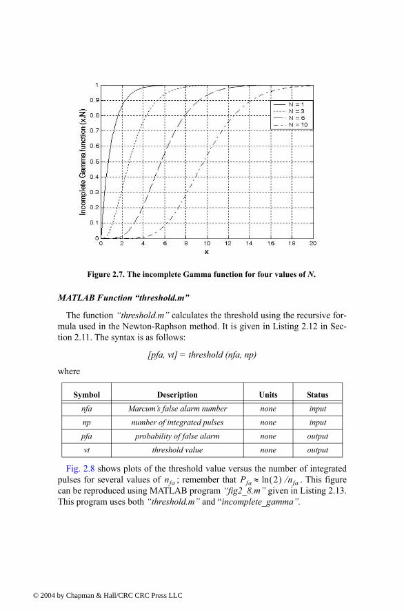
© 200
MATLAB Function threshold.m
The function threshold.m calculates the threshold using the recursive for-mula used in the Newton-Raphson method. It is given in Listing 2.12 in Sec-tion 2.11. The syntax is as follows:
[pfa, vt] = threshold (nfa, np)
where
Fig. 2.8 shows plots of the threshold value versus the number of integrated pulses for several values of ; remember that . This figure can be reproduced using MATLAB program fig2_8.m given in Listing 2.13. This program uses both threshold.m and incomplete_gamma.
Symbol Description Units Status
nfa Marcums false alarm number none input
np number of integrated pulses none input
pfa probability of false alarm none output
vt threshold value none output
Figure 2.7. The incomplete Gamma function for four values of N.
nfa Pfa 2( )ln nfa⁄≈
4 by Chapman & Hall/CRC CRC Press LLC
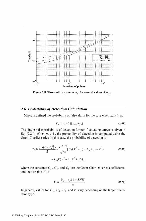
© 200
2.6. Probability of Detection CalculationMarcum defined the probability of false alarm for the case when as
(2.68)
The single pulse probability of detection for non-fluctuating targets is given in Eq. (2.24). When , the probability of detection is computed using the Gram-Charlier series. In this case, the probability of detection is
(2.69)
where the constants , , and are the Gram-Charlier series coefficients, and the variable is
(2.70)
In general, values for , , , and vary depending on the target fluctu-ation type.
Figure 2.8. Threshold versus for several values of .VT np nfa
nP 1>
Pfa 2( )ln nP nfa⁄( )≈
nP 1>
PDerfc V 2⁄( )
2------------------------------ e V2 2⁄
2π-------------- C3 V2 1( ) C4V 3 V2( )
C6V V4 10V2 15+( )
+[
]
≅
C3 C4 C6V
VVT nP 1 SNR+( )
ϖ--------------------------------------------=
C3 C4 C6 ϖ
4 by Chapman & Hall/CRC CRC Press LLC
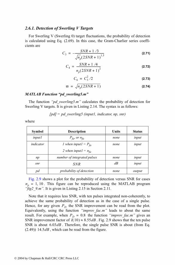
© 200
2.6.1. Detection of Swerling V Targets
For Swerling V (Swerling 0) target fluctuations, the probability of detection is calculated using Eq. (2.69). In this case, the Gram-Charlier series coeffi-cients are
(2.71)
(2.72)
(2.73)
(2.74)
MATLAB Function pd_swerling5.m
The function pd_swerling5.m calculates the probability of detection for Swerling V targets. It is given in Listing 2.14. The syntax is as follows:
[pd] = pd_swerling5 (input1, indicator, np, snr)
where
Fig. 2.9 shows a plot for the probability of detection versus SNR for cases . This figure can be reproduced using the MATLAB program
fig2_9.m. It is given in Listing 2.15 in Section 2.11.
Note that it requires less SNR, with ten pulses integrated non-coherently, to achieve the same probability of detection as in the case of a single pulse. Hence, for any given the SNR improvement can be read from the plot. Equivalently, using the function improv_fac.m leads to about the same result. For example, when the function improv_fac.m gives an SNR improvement factor of . Fig. 2.9 shows that the ten pulse SNR is about . Therefore, the single pulse SNR is about (from Eq. (2.49)) , which can be read from the figure.
Symbol Description Units Status
input1 Pfa, or nfa none input
indicator 1 when input1 = Pfa
2 when input1 = nfa
none input
np number of integrated pulses none input
snr dB input
pd probability of detection none output
C3SNR 1 3⁄+
np 2SNR 1+( )1.5--------------------------------------------=
C4SNR 1 4⁄+
np 2SNR 1+( )2-------------------------------------=
C6 C32 2⁄=
ϖ np 2SNR 1+( )=
SNR
np 1 10,=
PD
PD 0.8=I 10( ) 8.55dB≈
6.03dB14.5dB
4 by Chapman & Hall/CRC CRC Press LLC
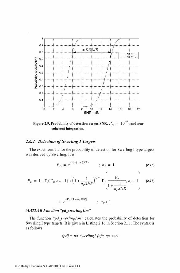
© 200
2.6.2. Detection of Swerling I Targets
The exact formula for the probability of detection for Swerling I type targets was derived by Swerling. It is
(2.75)
(2.76)
MATLAB Function pd_swerling1.m
The function pd_swerling1.m calculates the probability of detection for Swerling I type targets. It is given in Listing 2.16 in Section 2.11. The syntax is as follows:
[pd] = pd_swerling1 (nfa, np, snr)
Figure 2.9. Probability of detection versus SNR, , and non-coherent integration.
Pfa 10 9=
8.55dB≈
PD eVT 1 SNR+( )⁄
= nP; 1=
PD 1 ΓI VT nP 1,( ) 1 1nPSNR-----------------+
np 1ΓI
VT
1 1nPSNR-----------------+
--------------------------- nP 1,
×
+
eVT 1 nPSNR+( )⁄
=
nP 1>;
4 by Chapman & Hall/CRC CRC Press LLC
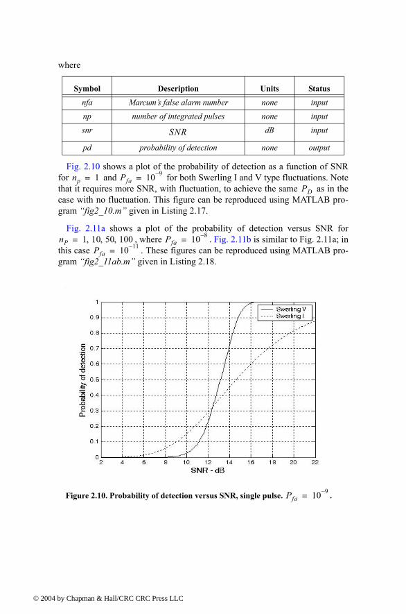
© 200
where
Fig. 2.10 shows a plot of the probability of detection as a function of SNR for and for both Swerling I and V type fluctuations. Note that it requires more SNR, with fluctuation, to achieve the same as in the case with no fluctuation. This figure can be reproduced using MATLAB pro-gram fig2_10.m given in Listing 2.17.
Fig. 2.11a shows a plot of the probability of detection versus SNR for , where . Fig. 2.11b is similar to Fig. 2.11a; in
this case . These figures can be reproduced using MATLAB pro-gram fig2_11ab.m given in Listing 2.18.
Symbol Description Units Status
nfa Marcums false alarm number none input
np number of integrated pulses none input
snr dB input
pd probability of detection none output
SNR
np 1= Pfa 10 9=PD
nP 1 10 50 100, , ,= Pfa 10 8=Pfa 10 11=
Figure 2.10. Probability of detection versus SNR, single pulse. .Pfa 10 9=
4 by Chapman & Hall/CRC CRC Press LLC
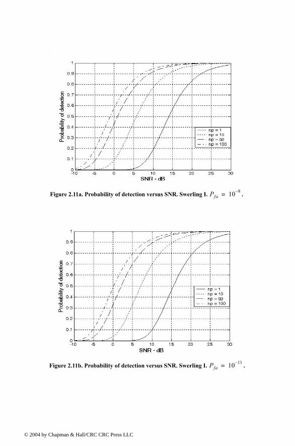
© 200
Figure 2.11a. Probability of detection versus SNR. Swerling I. .Pfa 10 8=
Figure 2.11b. Probability of detection versus SNR. Swerling I. .Pfa 10 11=
4 by Chapman & Hall/CRC CRC Press LLC
© 200
2.6.3. Detection of Swerling II Targets
In the case of Swerling II targets, the probability of detection is given by
(2.77)
For the case when Eq. (2.69) is used to compute the probability of detection. In this case,
(2.78)
(2.79)
(2.80)
MATLAB Function pd_swerling2.m
The function pd_swerling2.m calculates for Swerling II type targets. It is given in Listing 2.19 in Section 2.11. The syntax is as follows:
[pd] = pd_swerling2 (nfa, np, snr)
where
Fig. 2.12 shows a plot of the probability of detection as a function of SNR for , where . This figure can be reproduced using MATLAB program fig2_12.m given in Listing 2.20.
2.6.4. Detection of Swerling III Targets
The exact formulas, developed by Marcum, for the probability of detection for Swerling III type targets when is
(2.81)
Symbol Description Units Status
nfa Marcums false alarm number none input
np number of integrated pulses none input
snr dB input
pd probability of detection none output
PD 1 ΓIVT
1 SNR+( )------------------------- np, = nP 50≤;
nP 50>
C31
3 np
------------= C6,C3
2
2------=
C41
4nP---------=
ϖ nP 1 SNR+( )=
PD
SNR
nP 1 10 50 100, , ,= Pfa 10 10=
nP 1 2,=
PDVT
1 nPSNR 2⁄+--------------------------------- 1 2
nPSNR-----------------+
nP 2K0×exp=
K0 1VT
1 nPSNR 2⁄+--------------------------------- 2
nPSNR----------------- nP 2( )+=
4 by Chapman & Hall/CRC CRC Press LLC
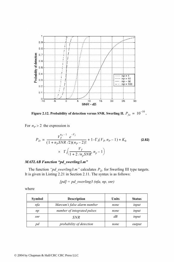
© 200
For the expression is
(2.82)
MATLAB Function pd_swerling3.m
The function pd_swerling3.m calculates for Swerling III type targets. It is given in Listing 2.21 in Section 2.11. The syntax is as follows:
[pd] = pd_swerling3 (nfa, np, snr)
where
Symbol Description Units Status
nfa Marcums false alarm number none input
np number of integrated pulses none input
snr dB input
pd probability of detection none output
Figure 2.12. Probability of detection versus SNR. Swerling II. .Pfa 10 10=
nP 2>
PDVT
nP 1e
VT
1 nPSNR 2⁄+( ) nP 2( )!------------------------------------------------------------ 1 ΓI VT nP 1,( ) K0
× ΓIVT
1 2 npSNR⁄+--------------------------------- np 1,
+ +=
PD
SNR
4 by Chapman & Hall/CRC CRC Press LLC
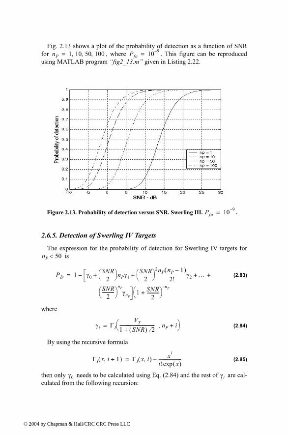
© 200
Fig. 2.13 shows a plot of the probability of detection as a function of SNR for , where . This figure can be reproduced using MATLAB program fig2_13.m given in Listing 2.22.
2.6.5. Detection of Swerling IV Targets
The expression for the probability of detection for Swerling IV targets for is
(2.83)
where
(2.84)
By using the recursive formula
(2.85)
then only needs to be calculated using Eq. (2.84) and the rest of are cal-culated from the following recursion:
nP 1 10 50 100, , ,= Pfa 10 9=
Figure 2.13. Probability of detection versus SNR. Swerling III. .Pfa 10 9=
nP 50<
PD 1 γ0SNR
2----------- nPγ1
SNR2
-----------
2nP nP 1( )2!
-------------------------γ2 …
SNR2
-----------
nP
γnP
+ + + +
1 SNR2
-----------+
nP
=
γi ΓIVT
1 SNR( ) 2⁄+-------------------------------- nP i+, =
ΓI x i 1+,( ) ΓI x i,( ) xi
i! x( )exp---------------------=
γ0 γi
4 by Chapman & Hall/CRC CRC Press LLC
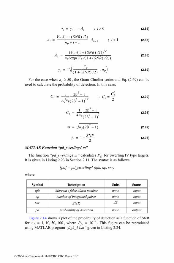
© 200
(2.86)
(2.87)
(2.88)
(2.89)
For the case when , the Gram-Charlier series and Eq. (2.69) can be used to calculate the probability of detection. In this case,
(2.90)
(2.91)
(2.92)
(2.93)
MATLAB Function pd_swerling4.m
The function pd_swerling4.m calculates for Swerling IV type targets. It is given in Listing 2.23 in Section 2.11. The syntax is as follows:
[pd] = pd_swerling4 (nfa, np, snr)
where
Figure 2.14 shows a plot of the probability of detection as a function of SNR for , where . This figure can be reproduced using MATLAB program fig2_14.m given in Listing 2.24.
Symbol Description Units Status
nfa Marcums false alarm number none input
np number of integrated pulses none input
snr dB input
pd probability of detection none output
γi γi 1 Ai= i 0>;
AiVT 1 SNR( ) 2⁄+( )⁄
nP i 1+----------------------------------------------- Ai 1= i 1>;
A1VT 1 SNR( ) 2⁄+( )⁄( )
nP
nP! VT 1 SNR( ) 2⁄+( )⁄( )exp----------------------------------------------------------------------=
γ0 ΓIVT
1 SNR( ) 2⁄+( )------------------------------------- nP, =
nP 50≥
C31
3 nP
------------- 2β3 1
2β2 1( )1.5
----------------------------= C6C3
2
2------=;
C41
4nP--------- 2β4 1
2β2 1( )2
-------------------------=
ϖ nP 2β2 1( )=
β 1 SNR2
-----------+=
PD
SNR
nP 1 10 50 100, , ,= Pfa 10 9=
4 by Chapman & Hall/CRC CRC Press LLC
© 200
2.7. The Radar Equation RevisitedThe radar equation developed in Chapter 1 assumed a constant target RCS
and did not account for integration loss. In this section, a more comprehensive form of the radar equation is introduced. In this case, the radar equation is given by
(2.94)
where is the average transmitted power, is the peak transmit-ted power, is pulsewidth, is PRF, is transmitting antenna gain, is receiving antenna gain, is wavelength, is target cross section, is improvement factor, is the number of integrated pulses, is Boltzmans constant, is effective noise temperature, is the system noise figure, is receiver bandwidth, is total system losses including integration loss, is loss due to target fluctuation, and is the minimum single pulse SNR required for detection.
The fluctuation loss, , can be viewed as the amount of additional SNR required to compensate for the SNR loss due to target fluctuation, given a spe-cific value. This was demonstrated for a Swerling I fluctuation in Fig.
Figure 2.14. Probability of detection versus SNR. Swerling IV. .Pfa 10 9=
R4 PavGtGrλ2σI nP( )
4π( )3kTeFBτfrLtLf SNR( )1----------------------------------------------------------------------=
Pav Ptτfr= Ptτ fr Gt Gr
λ σ I nP( )nP k
Te F BLt Lf
SNR( )1
Lf
PD
4 by Chapman & Hall/CRC CRC Press LLC
© 200
2.10. Kanter1 developed an exact analysis for calculating the fluctuation loss. In this text the authors will take advantage of the computational power of MATLAB and the MATLAB functions developed for this text to numerically calculate the amount of fluctuation loss with an accuracy of or better. For this purpose the MATLAB function fluct_loss.m was developed. It is given in Listing 2.25 in Section 2.11. Its syntax is as follows:
[Lf, Pd_Sw5] = fluct_loss(pd, pfa, np, sw_case)where
For example, using the syntax
[Lf,Pd_Sw5]=fluct_loss(0.65, 1e-9, 10,1)
will calculate the corresponding to both Swerling V and Swerling I fluc-tuation when the desired probability of detection and probability of false alarm and 10 pulses of non-coherent integration. The fol-lowing is a reprint of the output:
PD_SW5 = 0.65096989459928SNR_SW5 = 5.52499999999990PD_SW1 = 0.65019653294095SNR_SW1 = 8.32999999999990
Lf = 2.80500000000000
Note that a negative value for indicates a fluctuation SNR gain instead of loss. Finally, it must be noted that the function fluct_loss.m always assumes non-coherent integration. Fig. 2.15 shows a plot for the additional SNR (or fluctuation loss) required to achieve a certain probability of detection. This fig-ure can be reproduced using MATLAB program fig2_16.m given in Listing 2.26 in Section 2.11.
1. Kanter, I., Exact Detection Probability for Partially Correlated Rayleigh Targets, IEEE Trans, AES-22, pp. 184-196, March 1986.
Symbol Description Units Status
pd desired probability of detection none input
pfa probability of false alarm none input
np number of pulses none input
sw_case 1, 2, 3, or 4 depending on the desired Swerling case
none input
Lf fluctuation loss dB output
Pd_Sw5 Probability of detection correspond-ing to a Swerling V case
none output
0.005dB
SNRPD 0.65=
Pfa 10 9=
Lf
4 by Chapman & Hall/CRC CRC Press LLC
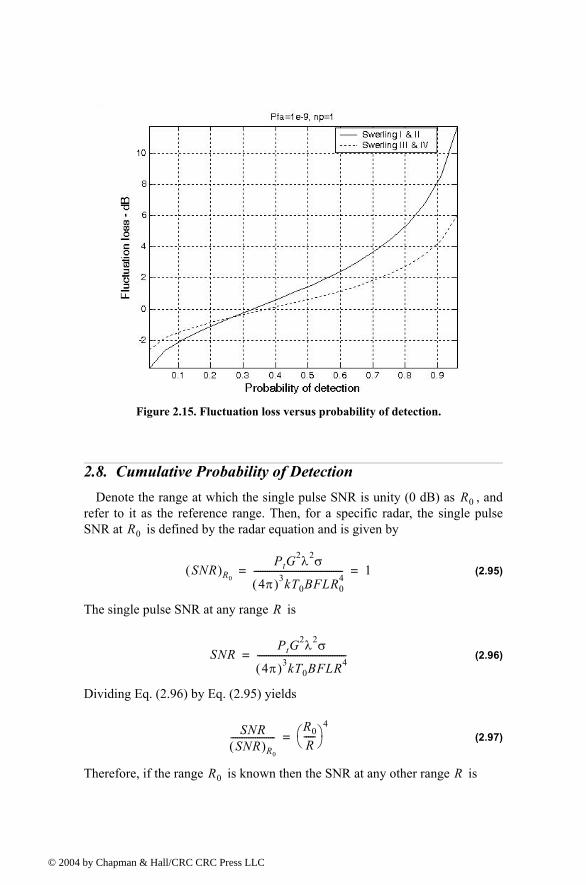
© 200
2.8. Cumulative Probability of DetectionDenote the range at which the single pulse SNR is unity (0 dB) as , and
refer to it as the reference range. Then, for a specific radar, the single pulse SNR at is defined by the radar equation and is given by
(2.95)
The single pulse SNR at any range is
(2.96)
Dividing Eq. (2.96) by Eq. (2.95) yields
(2.97)
Therefore, if the range is known then the SNR at any other range is
Figure 2.15. Fluctuation loss versus probability of detection.
R0
R0
SNR( )R0
PtG2λ2σ
4π( )3kT0BFLR04
---------------------------------------- 1= =
R
SNRPtG
2λ2σ
4π( )3kT0BFLR4----------------------------------------=
SNRSNR( )R0
--------------------R0
R-----
4=
R0 R
4 by Chapman & Hall/CRC CRC Press LLC
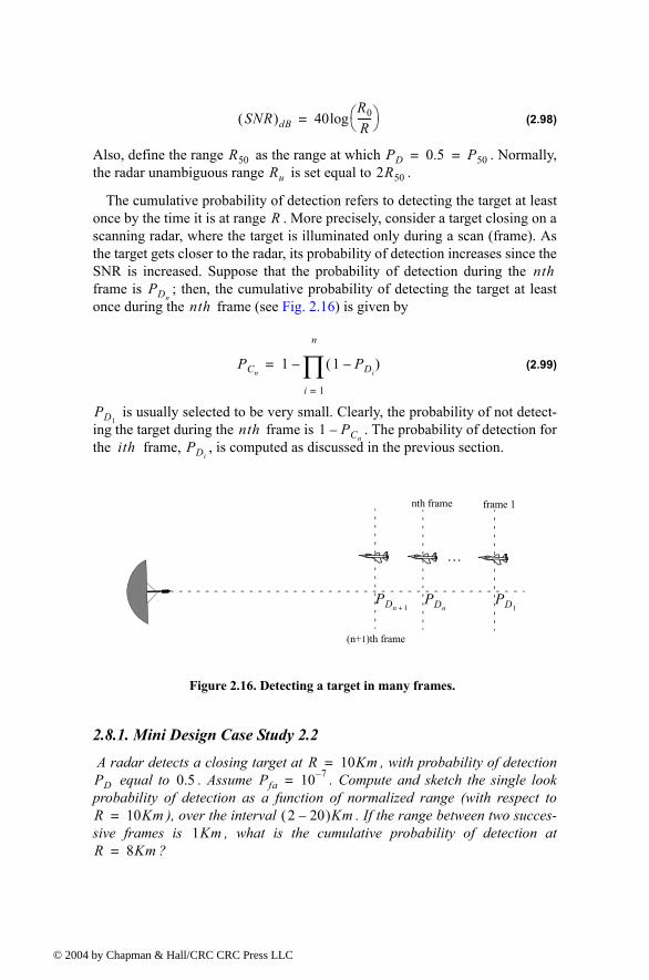
© 200
(2.98)
Also, define the range as the range at which . Normally, the radar unambiguous range is set equal to .
The cumulative probability of detection refers to detecting the target at least once by the time it is at range . More precisely, consider a target closing on a scanning radar, where the target is illuminated only during a scan (frame). As the target gets closer to the radar, its probability of detection increases since the SNR is increased. Suppose that the probability of detection during the frame is ; then, the cumulative probability of detecting the target at least once during the frame (see Fig. 2.16) is given by
(2.99)
is usually selected to be very small. Clearly, the probability of not detect-ing the target during the frame is . The probability of detection for the frame, , is computed as discussed in the previous section.
2.8.1. Mini Design Case Study 2.2
A radar detects a closing target at , with probability of detection equal to . Assume . Compute and sketch the single look
probability of detection as a function of normalized range (with respect to ), over the interval . If the range between two succes-
sive frames is , what is the cumulative probability of detection at ?
SNR( )dB 40R0
R----- log=
R50 PD 0.5 P50= =Ru 2R50
R
nthPDn
nth
PCn1 1 PDi
( )
i 1=
n
∏=
PD1nth 1 PCn
ith PDi
Figure 2.16. Detecting a target in many frames.
…
frame 1nth frame
(n+1)th frame
PD1PDn 1+
PDn
R 10Km=PD 0.5 Pfa 10 7=
R 10Km= 2 20( )Km1Km
R 8Km=
4 by Chapman & Hall/CRC CRC Press LLC
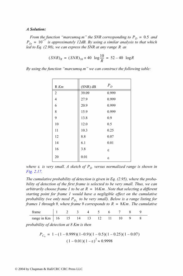
© 200
A Solution:
From the function marcumsq.m the SNR corresponding to and is approximately 12dB. By using a similar analysis to that which
led to Eq. (2.98), we can express the SNR at any range as
By using the function marcumsq.m we can construct the following table:
where is very small. A sketch of versus normalized range is shown in Fig. 2.17.
The cumulative probability of detection is given in Eq. (2.95), where the proba-bility of detection of the first frame is selected to be very small. Thus, we can arbitrarily choose frame 1 to be at . Note that selecting a different starting point for frame 1 would have a negligible effect on the cumulative probability (we only need to be very small). Below is a range listing for frames 1 through 9, where frame 9 corresponds to . The cumulative
probability of detection at 8 Km is then
R Km (SNR) dB
2 39.09 0.999
4 27.9 0.999
6 20.9 0.999
8 15.9 0.999
9 13.8 0.9
10 12.0 0.5
11 10.3 0.25
12 8.8 0.07
14 6.1 0.01
16 3.8
20 0.01
frame 1 2 3 4 5 6 7 8 9
range in Km 16 15 14 13 12 11 10 9 8
PD 0.5=Pfa 10 7=
R
SNR( )R SNR( )10 40 10R------log+ 52 40 Rlog= =
PD
ε
ε
ε PD
R 16Km=
PD1R 8Km=
PC91 1 0.999( ) 1 0.9( ) 1 0.5( ) 1 0.25( ) 1 0.07( )
1 0.01( ) 1 ε( )2 0.9998≈
=
4 by Chapman & Hall/CRC CRC Press LLC
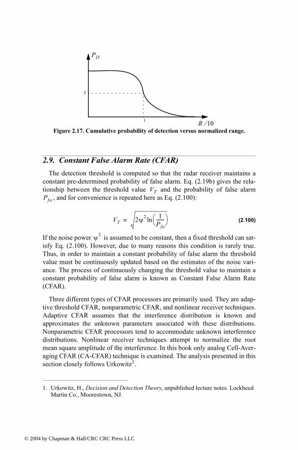
© 200
2.9. Constant False Alarm Rate (CFAR)The detection threshold is computed so that the radar receiver maintains a
constant pre-determined probability of false alarm. Eq. (2.19b) gives the rela-tionship between the threshold value and the probability of false alarm
, and for convenience is repeated here as Eq. (2.100):
(2.100)
If the noise power is assumed to be constant, then a fixed threshold can sat-isfy Eq. (2.100). However, due to many reasons this condition is rarely true. Thus, in order to maintain a constant probability of false alarm the threshold value must be continuously updated based on the estimates of the noise vari-ance. The process of continuously changing the threshold value to maintain a constant probability of false alarm is known as Constant False Alarm Rate (CFAR).
Three different types of CFAR processors are primarily used. They are adap-tive threshold CFAR, nonparametric CFAR, and nonlinear receiver techniques. Adaptive CFAR assumes that the interference distribution is known and approximates the unknown parameters associated with these distributions. Nonparametric CFAR processors tend to accommodate unknown interference distributions. Nonlinear receiver techniques attempt to normalize the root mean square amplitude of the interference. In this book only analog Cell-Aver-aging CFAR (CA-CFAR) technique is examined. The analysis presented in this section closely follows Urkowitz1.
1. Urkowitz, H., Decision and Detection Theory, unpublished lecture notes. Lockheed Martin Co., Moorestown, NJ.
R 10⁄
PD
1
.5
Figure 2.17. Cumulative probability of detection versus normalized range.
VTPfa
VT 2ψ2 1Pfa------- ln=
ψ2
4 by Chapman & Hall/CRC CRC Press LLC
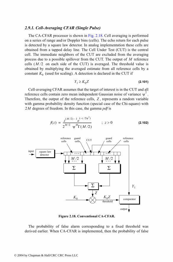
© 200
2.9.1. Cell-Averaging CFAR (Single Pulse)
The CA-CFAR processor is shown in Fig. 2.18. Cell averaging is performed on a series of range and/or Doppler bins (cells). The echo return for each pulse is detected by a square law detector. In analog implementation these cells are obtained from a tapped delay line. The Cell Under Test (CUT) is the central cell. The immediate neighbors of the CUT are excluded from the averaging process due to a possible spillover from the CUT. The output of reference cells ( on each side of the CUT) is averaged. The threshold value is obtained by multiplying the averaged estimate from all reference cells by a constant (used for scaling). A detection is declared in the CUT if
(2.101)
Cell-averaging CFAR assumes that the target of interest is in the CUT and all reference cells contain zero mean independent Gaussian noise of variance . Therefore, the output of the reference cells, , represents a random variable with gamma probability density function (special case of the Chi-square) with
degrees of freedom. In this case, the gamma pdf is
(2.102)
The probability of false alarm corresponding to a fixed threshold was derived earlier. When CA-CFAR is implemented, then the probability of false
MM 2⁄
K0
Y1 K0Z≥
ψ2
Z
2M
f z( ) z M 2⁄( ) 1 ez 2ψ2⁄( )
2M 2⁄ ψMΓ M 2⁄( )--------------------------------------------= z 0>;
Σ
… …
Σ…
Σ
K0 K0ZZ
Y1
M 2⁄ …M 2⁄
reference cells
reference cellsCUT
guardguard cells cells
input square law detector
comparator
output
threshold
Figure 2.18. Conventional CA-CFAR.
4 by Chapman & Hall/CRC CRC Press LLC
© 200
alarm can be derived from the conditional false alarm probability, which is averaged over all possible values of the threshold in order to achieve an uncon-ditional false alarm probability. The conditional probability of false alarm when can be written as
(2.103)
It follows that the unconditional probability of false alarm is
(2.104)
where is the pdf of the threshold, which except for the constant is the same as that defined in Eq. (2.102). Therefore,
(2.105)
Performing the integration in Eq. (2.104) yields
(2.106)
Observation of Eq. (2.106) shows that the probability of false alarm is now independent of the noise power, which is the objective of CFAR processing.
2.9.2. Cell-Averaging CFAR with Non-Coherent Integration
In practice, CFAR averaging is often implemented after non-coherent inte-gration, as illustrated in Fig. 2.19. Now, the output of each reference cell is the sum of squared envelopes. It follows that the total number of summed ref-erence samples is . The output is also the sum of squared enve-lopes. When noise alone is present in the CUT, is a random variable whose pdf is a gamma distribution with degrees of freedom. Additionally, the summed output of the reference cells is the sum of squared envelopes. Thus, is also a random variable which has a gamma pdf with degrees of freedom.
The probability of false alarm is then equal to the probability that the ratio exceeds the threshold. More precisely,
(2.107)
y VT=
Pfa VT y=( ) e y 2ψ2⁄=
Pfa Pfa VT y=( )f y( ) yd
0
∞
∫=
f y( ) K0
f y( ) yM 1 ey 2K0ψ
2⁄( )
2K0ψ2( )
MΓ M( )
---------------------------------------= ; y 0≥
Pfa1
1 K0+( )M------------------------=
nPMnP Y1 nP
Y12np
MnPZ 2MnP
Y1 Z⁄
Pfa Prob Y1 Z⁄ K1> =
4 by Chapman & Hall/CRC CRC Press LLC
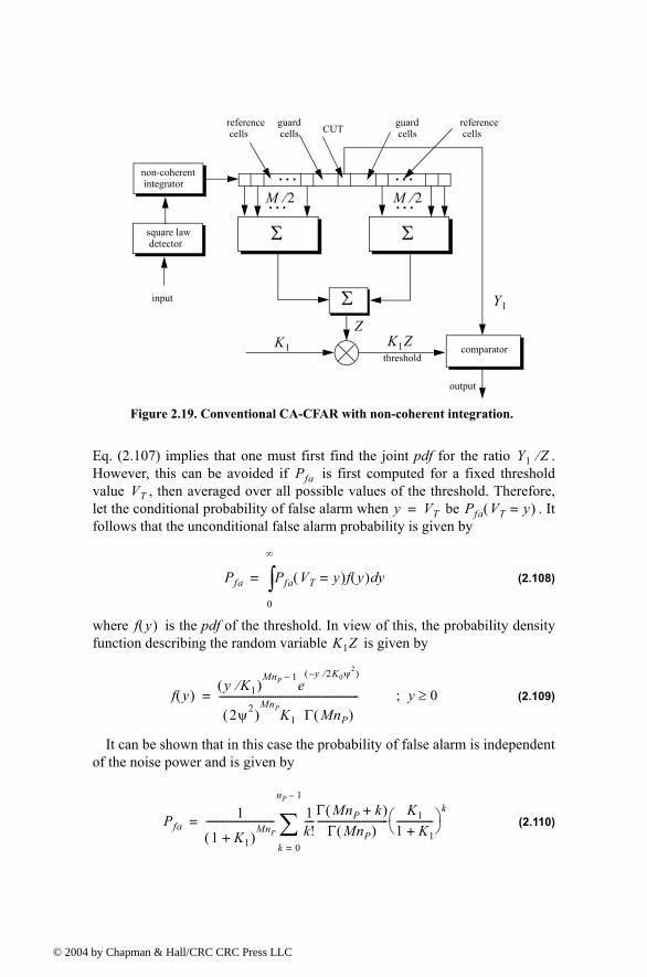
© 200
Eq. (2.107) implies that one must first find the joint pdf for the ratio . However, this can be avoided if is first computed for a fixed threshold value , then averaged over all possible values of the threshold. Therefore, let the conditional probability of false alarm when be . It follows that the unconditional false alarm probability is given by
(2.108)
where is the pdf of the threshold. In view of this, the probability density function describing the random variable is given by
(2.109)
It can be shown that in this case the probability of false alarm is independent of the noise power and is given by
(2.110)
Σ
… …
Σ…
Σ
K1 K1ZZ
Y1
M 2⁄ …M 2⁄
reference cells
reference cellsCUT
guardguard cells cells
non-coherent integrator
comparator
output
threshold
Figure 2.19. Conventional CA-CFAR with non-coherent integration.
square law detector
input
Y1 Z⁄Pfa
VTy VT= Pfa VT y=( )
Pfa Pfa VT y=( )f y( ) yd
0
∞
∫=
f y( )K1Z
f y( )y K1⁄( )
MnP 1e
y 2K0ψ2⁄( )
2ψ2( )MnPK1 Γ MnP( )
---------------------------------------------------------= ; y 0≥
Pfa1
1 K1+( )MnP
---------------------------- 1k!----Γ MnP k+( )Γ MnP( )
-----------------------------K1
1 K1+---------------
k
k 0=
nP 1
∑=
4 by Chapman & Hall/CRC CRC Press LLC
© 200
which is identical to Eq. (2.106) when and .
2.10. MyRadar Design Case Study - Visit 21
2.10.1. Problem StatementModify the design introduced in Chapter 1 for the MyRadar design case
study so that the effects of target RCS fluctuations are taken into account. For this purpose modify the design such that: The aircraft and missile target types follow Swerling I and Swerling III fluctuations, respectively. Also assume that a is required at maximum range with or better. You may use either non-coherent integration or cumulative probability of detection. Also, modify any other design parameters if needed.
2.10.2. A Design
The missile and the aircraft detection ranges were calculated in Chapter 1. They are for the aircraft and for the missile. First, determine the probability of detection for each target type with and without the 7-pulse non-coherent integration. For this purpose, use MATLAB program myradar_visit2_1.m given in Listing 2.27. This program first computes the improvement factor and the associated integration loss. Second it calculates the single pulse SNR. Finally it calculates the SNR when non-coherent integration is utilized. Executing this program yields:
SNR_single_pulse_missile = 5.5998 dBSNR_7_pulse_NCI_missile = 11.7216 dBSNR_single_pulse_aircraft = 6.0755 dB SNR_7_pulse_NCI_aircrfat = 12.1973 dB
Using these values in functions pd_swerling1.m and pd_swerling3.myields
Pd_single_pulse_missile = 0.013Pd_7_pulse_NCI_missile= 0.9276Pd_single_pulse_aircraft = 0.038Pd_7_pulse_NCI_aircraft = 0.8273
Clearly in all four cases, there is not enough SNR to meet the design require-ment of .
1. Please read disclaimer in Section 1.9.1.
K1 K0= nP 1=
PD 0.995≥ Pfa 10 7=
Ra 90Km= Rm 55Km=
PD 0.995≥
4 by Chapman & Hall/CRC CRC Press LLC
© 200
Instead, resort to accomplishing the desired probability of detection by using cumulative probabilities. The single frame increment for the missile and air-craft cases are
(2.111)
(2.112)
2.10.2.1 Single Pulse (Per Frame) Design Option
As a first design option, consider the case where during each frame only a single pulse is used for detection (i.e., no integration). Consequently, if the sin-gle pulse detection does not achieve the desired probability of detection at 90 Km for the aircraft or at 55 Km for the missile, then non-coherent integration of a few pulses per frame can then be utilized. Keep in mind that only non-coherent integration can be used in the cases of Swerling type I and III fluctua-tions (see Section 2.4).
Assume that the first frame corresponding to detecting the aircraft is 106 Km. This assumption is arbitrary and it provides the designer with 21 frames. It follows that the first frame, when detecting the missile, is at 61 Km. Further-more, assume that the SNR at is , for the aircraft case. And, for the missile case assume that at the corre-sponding SNR is . Note that these values are simply edu-cated guesses, and the designer may be required to perform several iterations in order to accomplish the desired cumulative probability of detection,
. In order to calculate the cumulative probability of detection at a certain range, the MATLAB program myradar_visit2_2.m was developed. This program is given in Listing 2.28 in Section 2.11.
Initialization of the program myradar_visit2_2.m includes entering the following inputs: The desired ; the number of pulses to be used for non-coherent integration per frame; the range at which the desired cumulative oper-ability of detection must be achieved; the frame size; and finally the target fluc-tuation type. For notational purposes, denote the range at which the desired cumulative probability of detection must be achieved as . Then for each frame, the following list includes the outputs of this program: SNR, probability of detection, fluctuation loss, and cumulative probability of detection.
The logic used by this program for calculating the proper probability of detection at each frame and for computing the cumulative probability of detec-tion is described as follows:
1. Initialize the program, by entering the desired input values. Assume Swer-ling V fluctuation and use Eq. (2.98) to calculate the frame-SNR, .
RMissile scan rate vm× 2 150× 300m= = =
RAircraft scan rate va× 2 400× 800m= = =
R 90Km= SNR( )aircraft 8.5dB=R 55Km=
SNR( )missile 9dB=
PD 0.995≥
Pfa
R0
SNR( )i
4 by Chapman & Hall/CRC CRC Press LLC
© 200
1.1. For the MyRadar design case study, use , , and
. Alternatively use and
for the missile case. Note that the selected SNR values are best estimates or educated guesses, and it may require going through few iterations before finally selecting an acceptable set.
2. The program will then calculate the number of frames and their associated ranges. The program uses the function fluct_loss.m to calculate the Swerling V at each frame and the additional SNR required to accom-plish the same probability of detection when target fluctuation is included.
3. Depending on the fluctuation type, the program will then use the proper MATLAB function to calculate the probability of detection for each frame,
.
3.1. For the MyRadar design case study, these functions are pd_swerling1.m and pd_swerling 3.m.
4. Finally, the program uses Eq. (2.99) to compute the cumulative probability of detection, .
A Graphical User Interface (GUI) has been developed for this program; Fig. 2.20 shows its associated GUI workspace. To use this GUI, from the MATLAB command window type myradar_visit2_2_gui. Executing the program myradar_visit2_2.m using the input values stated above yields the following cumulative probabilities of detection for the aircraft and missile cases,
These results clearly satisfy the design requirement of . However, one must re-validate the peak power requirement for the design. To do that, go back to Eq.s (1.107) and (1.108), and replace the SNR values used in Chapter 1 by the values adopted in this chapter (i.e., and
). It follows that the corresponding single pulse energy for the missile and the aircraft cases are respectively given by
(2.113)
(2.114)
nP 1= R0 90Km=
SNR0( )aircraft 8.5dB= R0 55Km=
SNR( )missile 9dB=
PD
PDi
PDn
PDCMissile0.99872=
PDCaircraft0.99687=
PD 0.995≥
SNR0( )aircraft 8.5dB=SNR( )missile 9dB=
Em 0.1658 100.9
100.56-------------× 0.36273Joules= =
Ea 0.1487 100.85
100.56-------------× 0.28994Joules= =
4 by Chapman & Hall/CRC CRC Press LLC
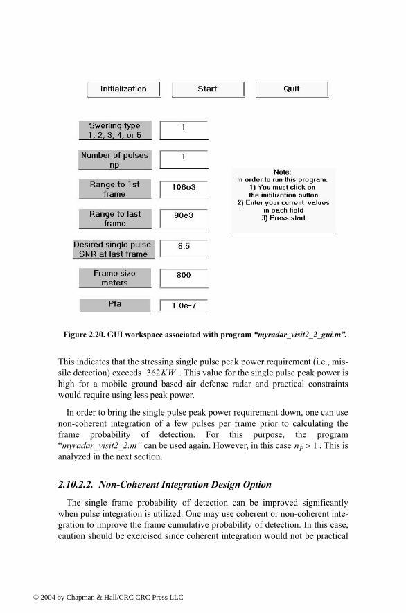
© 200
This indicates that the stressing single pulse peak power requirement (i.e., mis-sile detection) exceeds . This value for the single pulse peak power is high for a mobile ground based air defense radar and practical constraints would require using less peak power.
In order to bring the single pulse peak power requirement down, one can use non-coherent integration of a few pulses per frame prior to calculating the frame probability of detection. For this purpose, the program myradar_visit2_2.m can be used again. However, in this case . This is analyzed in the next section.
2.10.2.2. Non-Coherent Integration Design Option
The single frame probability of detection can be improved significantly when pulse integration is utilized. One may use coherent or non-coherent inte-gration to improve the frame cumulative probability of detection. In this case, caution should be exercised since coherent integration would not be practical
Figure 2.20. GUI workspace associated with program myradar_visit2_2_gui.m.
362KW
nP 1>
4 by Chapman & Hall/CRC CRC Press LLC
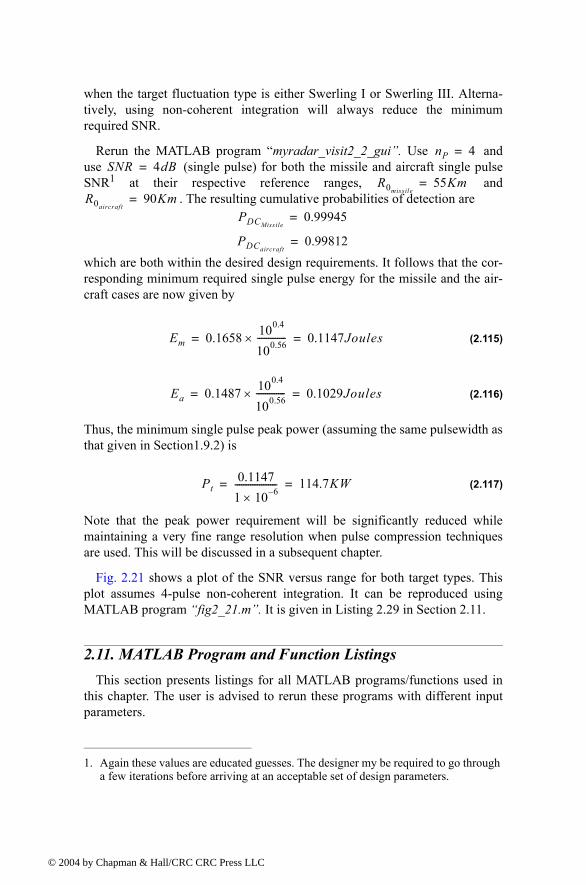
© 200
when the target fluctuation type is either Swerling I or Swerling III. Alterna-tively, using non-coherent integration will always reduce the minimum required SNR.
Rerun the MATLAB program myradar_visit2_2_gui. Use and use (single pulse) for both the missile and aircraft single pulse SNR1 at their respective reference ranges, and
. The resulting cumulative probabilities of detection are
which are both within the desired design requirements. It follows that the cor-responding minimum required single pulse energy for the missile and the air-craft cases are now given by
(2.115)
(2.116)
Thus, the minimum single pulse peak power (assuming the same pulsewidth as that given in Section1.9.2) is
(2.117)
Note that the peak power requirement will be significantly reduced while maintaining a very fine range resolution when pulse compression techniques are used. This will be discussed in a subsequent chapter.
Fig. 2.21 shows a plot of the SNR versus range for both target types. This plot assumes 4-pulse non-coherent integration. It can be reproduced using MATLAB program fig2_21.m. It is given in Listing 2.29 in Section 2.11.
2.11. MATLAB Program and Function ListingsThis section presents listings for all MATLAB programs/functions used in
this chapter. The user is advised to rerun these programs with different input parameters.
1. Again these values are educated guesses. The designer my be required to go through a few iterations before arriving at an acceptable set of design parameters.
nP 4=SNR 4dB=
R0missile55Km=
R0aircraft90Km=
PDCMissile0.99945=
PDCaircraft0.99812=
Em 0.1658 100.4
100.56-------------× 0.1147Joules= =
Ea 0.1487 100.4
100.56-------------× 0.1029Joules= =
Pt0.1147
1 10× 6------------------- 114.7KW= =
4 by Chapman & Hall/CRC CRC Press LLC
© 200
Listing 2.1. MATLAB Program fig2_2.m% This program can be used to reproduce Figure 2.2 of the textclear allclose allxg = linspace(-6,6,1500); % random variable between -6 and 6xr = linspace(0,6,1500); % random variable between 0 and 6mu = 0; % zero mean Gaussian pdf meansigma = 1.5; % standard deviation (sqrt(variance))ynorm = normpdf(xg,mu,sigma); % use MATLAB function normpdfyray = raylpdf(xr,sigma); % use MATLAB function raylpdfplot(xg,ynorm,'k',xr,yray,'k-.');gridlegend('Gaussian pdf','Rayleigh pdf')xlabel('x')
Figure 2.21. SNR versus detection range for both target types. The 4-pulse NCI curves correspond to 21 frame cumulative detection with the last frame at: 55 Km for the missile and 90 Km for the aircraft.
4 by Chapman & Hall/CRC CRC Press LLC

© 200
ylabel('Probability density')gtext('\mu = 0; \sigma = 1.5')gtext('\sigma =1.5')
Listing 2.2. MATLAB Function que_func.mfunction fofx = que_func(x)% This function computes the value of the Q-function% listed in Eq.(2.16). It uses the approximation in Eqs. (2.17) and (2.18)if (x >= 0) denom = 0.661 * x + 0.339 * sqrt(x^2 + 5.51); expo = exp(-x^2 /2.0); fofx = 1.0 - (1.0 / sqrt(2.0 * pi)) * (1.0 / denom) * expo;else denom = 0.661 * x + 0.339 * sqrt(x^2 + 5.51); expo = exp(-x^2 /2.0); value = 1.0 - (1.0 / sqrt(2.0 * pi)) * (1.0 / denom) * expo; fofx = 1.0 - value;end
Listing 2.3. MATLAB Program fig2_3.m%This program generates Figure 2.3.close allclear alllogpfa = linspace(.01,250,1000);var = 10.^(logpfa ./ 10.0);vtnorm = sqrt( log (var));semilogx(logpfa, vtnorm,'k')grid
Listing 2.4. MATLAB Function marcumsq.mfunction Pd = marcumsq (a,b)% This function uses Parl's method to compute PDmax_test_value = 5000.; if (a < b) alphan0 = 1.0; dn = a / b;else alphan0 = 0.; dn = b / a;endalphan_1 = 0.;betan0 = 0.5;
4 by Chapman & Hall/CRC CRC Press LLC
© 200
betan_1 = 0.;D1 = dn;n = 0;ratio = 2.0 / (a * b);r1 = 0.0;betan = 0.0;alphan = 0.0;while betan < 1000., n = n + 1; alphan = dn + ratio * n * alphan0 + alphan; betan = 1.0 + ratio * n * betan0 + betan; alphan_1 = alphan0; alphan0 = alphan; betan_1 = betan0; betan0 = betan; dn = dn * D1;endPD = (alphan0 / (2.0 * betan0)) * exp( -(a-b)^2 / 2.0);if ( a >= b) PD = 1.0 - PD;endreturn
Listing 2.5. MATLAB Program prob_snr1.m% This program is used to produce Fig. 2.4close allclear allfor nfa = 2:2:12 b = sqrt(-2.0 * log(10^(-nfa))); index = 0; hold on for snr = 0:.1:18 index = index +1; a = sqrt(2.0 * 10^(.1*snr)); pro(index) = marcumsq(a,b); end x = 0:.1:18; set(gca,'ytick',[.1 .2 .3 .4 .5 .6 .7 .75 .8 .85 .9 ... .95 .9999]) set(gca,'xtick',[1 2 3 4 5 6 7 8 9 10 11 12 13 14 15 16 17 18])
loglog(x, pro,'k');end
4 by Chapman & Hall/CRC CRC Press LLC
© 200
hold offxlabel ('Single pulse SNR - dB')ylabel ('Probability of detection')grid
Listing 2.6. MATLAB program fig2_6a.m % This program is used to produce Fig. 2.6a% It uses the function "improv_fac"clear allclose allpfa1 = 1.0e-2;pfa2 = 1.0e-6;pfa3 = 1.0e-10;pfa4 = 1.0e-13;pd1 = .5;pd2 = .8;pd3 = .95;pd4 = .999;index = 0;for np = 1:1:1000 index = index + 1; I1(index) = improv_fac (np, pfa1, pd1); I2(index) = improv_fac (np, pfa2, pd2); I3(index) = improv_fac (np, pfa3, pd3); I4(index) = improv_fac (np, pfa4, pd4);endnp = 1:1:1000;semilogx (np, I1, 'k', np, I2, 'k--', np, I3, 'k-.', np, I4, 'k:')xlabel ('Number of pulses');ylabel ('Improvement factor I - dB')legend ('pd=.5, nfa=e+2','pd=.8, nfa=e+6','pd=.95, nfa=e+10','pd=.999, nfa=e+13');grid
Listing 2.7. MATLAB Function improv_fac.mfunction impr_of_np = improv_fac (np, pfa, pd)% This function computes the non-coherent integration improvement% factor using the empirical formula defined in Eq. (2.49)fact1 = 1.0 + log10( 1.0 / pfa) / 46.6;fact2 = 6.79 * (1.0 + 0.235 * pd);fact3 = 1.0 - 0.14 * log10(np) + 0.0183 * (log10(np))^2;
4 by Chapman & Hall/CRC CRC Press LLC
© 200
impr_of_np = fact1 * fact2 * fact3 * log10(np);return
Listing 2.8. MATLAB Program fig2_6b.m% This program is used to produce Fig. 2.6b% It uses the function "improv_fac". clear allclose allpfa1 = 1.0e-12;pfa2 = 1.0e-12;pfa3 = 1.0e-12;pfa4 = 1.0e-12;pd1 = .5;pd2 = .8;pd3 = .95;pd4 = .99;index = 0;for np = 1:1:1000 index = index+1; I1 = improv_fac (np, pfa1, pd1); i1 = 10.^(0.1*I1); L1(index) = -1*10*log10(i1 ./ np); I2 = improv_fac (np, pfa2, pd2); i2 = 10.^(0.1*I2); L2(index) = -1*10*log10(i2 ./ np); I3 = improv_fac (np, pfa3, pd3); i3 = 10.^(0.1*I3); L3(index) = -1*10*log10(i3 ./ np); I4 = improv_fac (np, pfa4, pd4); i4 = 10.^(0.1*I4); L4 (index) = -1*10*log10(i4 ./ np);endnp = 1:1:1000;semilogx (np, L1, 'k', np, L2, 'k--', np, L3, 'k-.', np, L4, 'k:')axis tightxlabel ('Number of pulses');ylabel ('Integration loss - dB')legend ('pd=.5, nfa=e+12','pd=.8, nfa=e+12','pd=.95, nfa=e+12','pd=.99, nfa=e+12');grid
4 by Chapman & Hall/CRC CRC Press LLC
© 200
Listing 2.9. MATLAB Function incomplete_gamma.mfunction [value] = incomplete_gamma ( vt, np)% This function implements Eq. (2.67) to compute the Incomplete Gamma Function% This function needs "factor.m" to runformat longeps = 1.000000001;% Test to see if np = 1if (np == 1) value1 = vt * exp(-vt); value = 1.0 - exp(-vt); returnendsumold = 1.0;sumnew =1.0;calc1 = 1.0;calc2 = np;xx = np * log(vt+0.0000000001) - vt - factor(calc2);temp1 = exp(xx);temp2 = np / (vt+0.0000000001);diff = .0;ratio = 1000.0;if (vt >= np) while (ratio >= eps) diff = diff + 1.0; calc1 = calc1 * (calc2 - diff) / vt ; sumnew = sumold + calc1; ratio = sumnew / sumold; sumold = sumnew; end value = 1.0 - temp1 * sumnew * temp2; return else diff = 0.; sumold = 1.; ratio = 1000.; calc1 = 1.; while(ratio >= eps) diff = diff + 1.0; calc1 = calc1 * vt / (calc2 + diff); sumnew = sumold + calc1; ratio = sumnew / sumold; sumold = sumnew;
4 by Chapman & Hall/CRC CRC Press LLC
© 200
end value = temp1 * sumnew;end
Listing 2.10. MATLAB Function factor.mfunction [val] = factor(n)% Compute the factorial of n using logarithms to avoid overflow.format longn = n + 9.0;n2 = n * n;temp = (n-1) * log(n) - n + log(sqrt(2.0 * pi * n)) ... + ((1.0 - (1.0/30. + (1.0/105)/n2)/n2) / 12) / n;val = temp - log((n-1)*(n-2)*(n-3)*(n-4)*(n-5)*(n-6) ... *(n-7)*(n-8));return
Listing 2.11. MATLAB Program fig2_7.m% This program can be used to reproduce Fig. 2.7close allclear allformat longii = 0;for x = 0:.1:20 ii = ii+1; val1(ii) = incomplete_gamma(x , 1); val2(ii) = incomplete_gamma(x , 3); val = incomplete_gamma(x , 6); val3(ii) = val; val = incomplete_gamma(x , 10); val4(ii) = val;endxx = 0:.1:20;plot(xx,val1,'k',xx,val2,'k:',xx,val3,'k--',xx,val4,'k-.')legend('N = 1','N = 3','N = 6','N = 10')xlabel('x')ylabel('Incomplete Gamma function (x,N)')grid
Listing 2.12. MATLAB Function threshold.mfunction [pfa, vt] = threshold (nfa, np)% This function calculates the threshold value from nfa and np.% The Newton-Raphson recursive formula is used (Eqs. (2-63) through (2-66))
4 by Chapman & Hall/CRC CRC Press LLC
© 200
% This function uses "incomplete_gamma.m".delmax = .00001;eps = 0.000000001;delta =10000.;pfa = np * log(2) / nfa;sqrtpfa = sqrt(-log10(pfa));sqrtnp = sqrt(np); vt0 = np - sqrtnp + 2.3 * sqrtpfa * (sqrtpfa + sqrtnp - 1.0);vt = vt0;while (abs(delta) >= vt0) igf = incomplete_gamma(vt0,np); num = 0.5^(np/nfa) - igf; temp = (np-1) * log(vt0+eps) - vt0 - factor(np-1); deno = exp(temp); vt = vt0 + (num / (deno+eps)); delta = abs(vt - vt0) * 10000.0; vt0 = vt;end
Listing 2.13. MATLAB Program fig2_8.m% Use this program to reproduce Fig. 2.8 of textclear allfor n= 1: 1:150 [pfa1 y1(n)] = threshold(1000,n); [pfa2 y3(n)] = threshold(10000,n); [pfa3 y4(n)] = threshold(500000,n);endn =1:1:150;loglog(n,y1,'k',n,y3,'k--',n,y4,'k-.');axis([0 200 1 300])xlabel ('Number of pulses');ylabel('Threshold')legend('nfa=1000','nfa=10000','nfa=500000')grid
Listing 2.14. MATLAB Function pd_swerling5.mfunction pd = pd_swerling5 (input1, indicator, np, snrbar)% This function is used to calculate the probability of % for Swerling 5 or 0 targets for np>1.if(np == 1) 'Stop, np must be greater than 1' return
4 by Chapman & Hall/CRC CRC Press LLC
© 200
endformat longsnrbar = 10.0.^(snrbar./10.);eps = 0.00000001;delmax = .00001;delta =10000.;% Calculate the threshold Vtif (indicator ~=1) nfa = input1; pfa = np * log(2) / nfa;else pfa = input1; nfa = np * log(2) / pfa;endsqrtpfa = sqrt(-log10(pfa));sqrtnp = sqrt(np); vt0 = np - sqrtnp + 2.3 * sqrtpfa * (sqrtpfa + sqrtnp - 1.0);vt = vt0;while (abs(delta) >= vt0) igf = incomplete_gamma(vt0,np); num = 0.5^(np/nfa) - igf; temp = (np-1) * log(vt0+eps) - vt0 - factor(np-1); deno = exp(temp); vt = vt0 + (num / (deno+eps)); delta = abs(vt - vt0) * 10000.0; vt0 = vt;end% Calculate the Gram-Charlier coefficientstemp1 = 2.0 .* snrbar + 1.0;omegabar = sqrt(np .* temp1);c3 = -(snrbar + 1.0 / 3.0) ./ (sqrt(np) .* temp1.^1.5);c4 = (snrbar + 0.25) ./ (np .* temp1.^2.);c6 = c3 .* c3 ./2.0;V = (vt - np .* (1.0 + snrbar)) ./ omegabar;Vsqr = V .*V;val1 = exp(-Vsqr ./ 2.0) ./ sqrt( 2.0 * pi);val2 = c3 .* (V.^2 -1.0) + c4 .* V .* (3.0 - V.^2) -... c6 .* V .* (V.^4 - 10. .* V.^2 + 15.0);q = 0.5 .* erfc (V./sqrt(2.0));pd = q - val1 .* val2;
4 by Chapman & Hall/CRC CRC Press LLC
© 200
Listing 2.15. MATLAB Program fig2_9.m% This program is used to produce Fig. 2.9close allclear allpfa = 1e-9;nfa = log(2) / pfa;b = sqrt(-2.0 * log(pfa));index = 0;for snr = 0:.1:20 index = index +1; a = sqrt(2.0 * 10^(.1*snr)); pro(index) = marcumsq(a,b); prob205(index) = pd_swerling5 (pfa, 1, 10, snr);endx = 0:.1:20;plot(x, pro,'k',x,prob205,'k:');axis([0 20 0 1])xlabel ('SNR - dB')ylabel ('Probability of detection')legend('np = 1','np = 10')grid
Listing 2.16. MATLAB Function pd_swerling1.mfunction pd = pd_swerling1 (nfa, np, snrbar)% This function is used to calculate the probability of detection% for Swerling 1 targets.format longsnrbar = 10.0^(snrbar/10.);eps = 0.00000001;delmax = .00001;delta =10000.;% Calculate the threshold Vtpfa = np * log(2) / nfa;sqrtpfa = sqrt(-log10(pfa));sqrtnp = sqrt(np); vt0 = np - sqrtnp + 2.3 * sqrtpfa * (sqrtpfa + sqrtnp - 1.0);vt = vt0;while (abs(delta) >= vt0) igf = incomplete_gamma(vt0,np); num = 0.5^(np/nfa) - igf; temp = (np-1) * log(vt0+eps) - vt0 - factor(np-1); deno = exp(temp);
4 by Chapman & Hall/CRC CRC Press LLC
© 200
vt = vt0 + (num / (deno+eps)); delta = abs(vt - vt0) * 10000.0; vt0 = vt;endif (np == 1) temp = -vt / (1.0 + snrbar); pd = exp(temp); returnend temp1 = 1.0 + np * snrbar; temp2 = 1.0 / (np *snrbar); temp = 1.0 + temp2; val1 = temp^(np-1.); igf1 = incomplete_gamma(vt,np-1); igf2 = incomplete_gamma(vt/temp,np-1); pd = 1.0 - igf1 + val1 * igf2 * exp(-vt/temp1);
Listing 2.17. MATLAB Program fig2_10.m% This program is used to reproduce Fig. 2.10close allclear allpfa = 1e-9;nfa = log(2) / pfa;b = sqrt(-2.0 * log(pfa));index = 0;for snr = 0:.1:22 index = index +1; a = sqrt(2.0 * 10^(.1*snr)); pro(index) = marcumsq(a,b); prob(index) = pd_swerling1 (nfa, 1, snr);endx = 0:.1:22;plot(x, pro,'k',x,prob,'k:');axis([2 22 0 1])xlabel ('SNR - dB')ylabel ('Probability of detection')legend('Swerling V','Swerling I')grid
4 by Chapman & Hall/CRC CRC Press LLC
© 200
Listing 2.18. MATLAB Program fig2_11ab.m% This program is used to produce Fig. 2.11a&bclear allpfa = 1e-11;nfa = log(2) / pfa;index = 0;for snr = -10:.5:30 index = index +1; prob1(index) = pd_swerling1 (nfa, 1, snr); prob10(index) = pd_swerling1 (nfa, 10, snr); prob50(index) = pd_swerling1 (nfa, 50, snr); prob100(index) = pd_swerling1 (nfa, 100, snr);endx = -10:.5:30;plot(x, prob1,'k',x,prob10,'k:',x,prob50,'k--', ... x, prob100,'k-.');axis([-10 30 0 1])xlabel ('SNR - dB')ylabel ('Probability of detection')legend('np = 1','np = 10','np = 50','np = 100')grid
Listing 2.19. MATLAB Function pd_swerling2.mfunction pd = pd_swerling2 (nfa, np, snrbar)% This function is used to calculate the probability of detection% for Swerling 2 targets.format longsnrbar = 10.0^(snrbar/10.);eps = 0.00000001;delmax = .00001;delta =10000.;% Calculate the threshold Vtpfa = np * log(2) / nfa;sqrtpfa = sqrt(-log10(pfa));sqrtnp = sqrt(np); vt0 = np - sqrtnp + 2.3 * sqrtpfa * (sqrtpfa + sqrtnp - 1.0);vt = vt0;while (abs(delta) >= vt0) igf = incomplete_gamma(vt0,np); num = 0.5^(np/nfa) - igf; temp = (np-1) * log(vt0+eps) - vt0 - factor(np-1); deno = exp(temp); vt = vt0 + (num / (deno+eps));
4 by Chapman & Hall/CRC CRC Press LLC
© 200
delta = abs(vt - vt0) * 10000.0; vt0 = vt;endif (np <= 50) temp = vt / (1.0 + snrbar); pd = 1.0 - incomplete_gamma(temp,np); returnelse temp1 = snrbar + 1.0; omegabar = sqrt(np) * temp1; c3 = -1.0 / sqrt(9.0 * np); c4 = 0.25 / np; c6 = c3 * c3 /2.0; V = (vt - np * temp1) / omegabar; Vsqr = V *V; val1 = exp(-Vsqr / 2.0) / sqrt( 2.0 * pi); val2 = c3 * (V^2 -1.0) + c4 * V * (3.0 - V^2) - ... c6 * V * (V^4 - 10. * V^2 + 15.0); q = 0.5 * erfc (V/sqrt(2.0)); pd = q - val1 * val2;end
Listing 2.20. MATLAB Program fig2_12.m% This program is used to produce Fig. 2.12clear allpfa = 1e-10;nfa = log(2) / pfa;index = 0;for snr = -10:.5:30 index = index +1; prob1(index) = pd_swerling2 (nfa, 1, snr); prob10(index) = pd_swerling2 (nfa, 10, snr); prob50(index) = pd_swerling2 (nfa, 50, snr); prob100(index) = pd_swerling2 (nfa, 100, snr);endx = -10:.5:30;plot(x, prob1,'k',x,prob10,'k:',x,prob50,'k--', ... x, prob100,'k-.');axis([-10 30 0 1])xlabel ('SNR - dB')ylabel ('Probability of detection')legend('np = 1','np = 10','np = 50','np = 100')grid
4 by Chapman & Hall/CRC CRC Press LLC
© 200
Listing 2.21. MATLAB Function pd_swerling3.mfunction pd = pd_swerling3 (nfa, np, snrbar)% This function is used to calculate the probability of detection% for Swerling 3 targets.format longsnrbar = 10.0^(snrbar/10.);eps = 0.00000001;delmax = .00001;delta =10000.;% Calculate the threshold Vtpfa = np * log(2) / nfa;sqrtpfa = sqrt(-log10(pfa));sqrtnp = sqrt(np); vt0 = np - sqrtnp + 2.3 * sqrtpfa * (sqrtpfa + sqrtnp - 1.0);vt = vt0;while (abs(delta) >= vt0) igf = incomplete_gamma(vt0,np); num = 0.5^(np/nfa) - igf; temp = (np-1) * log(vt0+eps) - vt0 - factor(np-1); deno = exp(temp); vt = vt0 + (num / (deno+eps)); delta = abs(vt - vt0) * 10000.0; vt0 = vt;endtemp1 = vt / (1.0 + 0.5 * np *snrbar);temp2 = 1.0 + 2.0 / (np * snrbar);temp3 = 2.0 * (np - 2.0) / (np * snrbar);ko = exp(-temp1) * temp2^(np-2.) * (1.0 + temp1 - temp3);if (np <= 2) pd = ko; returnelse temp4 = vt^(np-1.) * exp(-vt) / (temp1 * exp(factor(np-2.))); temp5 = vt / (1.0 + 2.0 / (np *snrbar)); pd = temp4 + 1.0 - incomplete_gamma(vt,np-1.) + ko * ... incomplete_gamma(temp5,np-1.);end
Listing 2.22. MATLAB Program fig2_13.m% This program is used to produce Fig. 2.13clear allpfa = 1e-9;
4 by Chapman & Hall/CRC CRC Press LLC
© 200
nfa = log(2) / pfa;index = 0;for snr = -10:.5:30 index = index +1; prob1(index) = pd_swerling3 (nfa, 1, snr); prob10(index) = pd_swerling3 (nfa, 10, snr); prob50(index) = pd_swerling3(nfa, 50, snr); prob100(index) = pd_swerling3 (nfa, 100, snr);endx = -10:.5:30;plot(x, prob1,'k',x,prob10,'k:',x,prob50,'k--', ... x, prob100,'k-.');axis([-10 30 0 1])xlabel ('SNR - dB')ylabel ('Probability of detection')legend('np = 1','np = 10','np = 50','np = 100')grid
Listing 2.23. MATLAB Function pd_swerling4.mfunction pd = pd_swerling4 (nfa, np, snrbar)% This function is used to calculate the probability of detection% for Swerling 4 targets.format longsnrbar = 10.0^(snrbar/10.);eps = 0.00000001;delmax = .00001;delta =10000.;% Calculate the threshold Vtpfa = np * log(2) / nfa;sqrtpfa = sqrt(-log10(pfa));sqrtnp = sqrt(np); vt0 = np - sqrtnp + 2.3 * sqrtpfa * (sqrtpfa + sqrtnp - 1.0);vt = vt0;while (abs(delta) >= vt0) igf = incomplete_gamma(vt0,np); num = 0.5^(np/nfa) - igf; temp = (np-1) * log(vt0+eps) - vt0 - factor(np-1); deno = exp(temp); vt = vt0 + (num / (deno+eps)); delta = abs(vt - vt0) * 10000.0; vt0 = vt;endh8 = snrbar /2.0;
4 by Chapman & Hall/CRC CRC Press LLC
© 200
beta = 1.0 + h8;beta2 = 2.0 * beta^2 - 1.0;beta3 = 2.0 * beta^3;if (np >= 50) temp1 = 2.0 * beta -1; omegabar = sqrt(np * temp1); c3 = (beta3 - 1.) / 3.0 / beta2 / omegabar; c4 = (beta3 * beta3 - 1.0) / 4. / np /beta2 /beta2; c6 = c3 * c3 /2.0; V = (vt - np * (1.0 + snrbar)) / omegabar; Vsqr = V *V; val1 = exp(-Vsqr / 2.0) / sqrt( 2.0 * pi); val2 = c3 * (V^2 -1.0) + c4 * V * (3.0 - V^2) - ... c6 * V * (V^4 - 10. * V^2 + 15.0); q = 0.5 * erfc (V/sqrt(2.0)); pd = q - val1 * val2; returnelse snr = 1.0; gamma0 = incomplete_gamma(vt/beta,np); a1 = (vt / beta)^np / (exp(factor(np)) * exp(vt/beta)); sum = gamma0; for i = 1:1:np temp1 = 1; if (i == 1) ai = a1; else ai = (vt / beta) * a1 / (np + i -1); end a1 = ai; gammai = gamma0 - ai; gamma0 = gammai; a1 = ai; for ii = 1:1:i temp1 = temp1 * (np + 1 - ii); end term = (snrbar /2.0)^i * gammai * temp1 / exp(factor(i)); sum = sum + term; end pd = 1.0 - sum / beta^np;endpd = max(pd,0.);
4 by Chapman & Hall/CRC CRC Press LLC
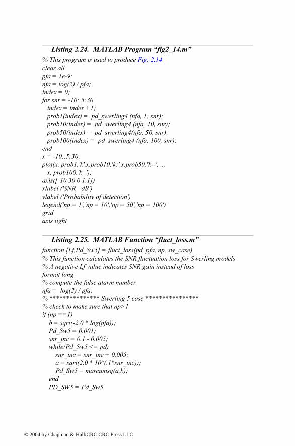
© 200
Listing 2.24. MATLAB Program fig2_14.m% This program is used to produce Fig. 2.14clear allpfa = 1e-9;nfa = log(2) / pfa;index = 0;for snr = -10:.5:30 index = index +1; prob1(index) = pd_swerling4 (nfa, 1, snr); prob10(index) = pd_swerling4 (nfa, 10, snr); prob50(index) = pd_swerling4(nfa, 50, snr); prob100(index) = pd_swerling4 (nfa, 100, snr);endx = -10:.5:30;plot(x, prob1,'k',x,prob10,'k:',x,prob50,'k--', ... x, prob100,'k-.');axis([-10 30 0 1.1])xlabel ('SNR - dB')ylabel ('Probability of detection')legend('np = 1','np = 10','np = 50','np = 100')gridaxis tight
Listing 2.25. MATLAB Function fluct_loss.mfunction [Lf,Pd_Sw5] = fluct_loss(pd, pfa, np, sw_case)% This function calculates the SNR fluctuation loss for Swerling models% A negative Lf value indicates SNR gain instead of loss format long% compute the false alarm numbernfa = log(2) / pfa;% *************** Swerling 5 case ****************% check to make sure that np>1if (np ==1) b = sqrt(-2.0 * log(pfa)); Pd_Sw5 = 0.001; snr_inc = 0.1 - 0.005; while(Pd_Sw5 <= pd) snr_inc = snr_inc + 0.005; a = sqrt(2.0 * 10^(.1*snr_inc)); Pd_Sw5 = marcumsq(a,b); end PD_SW5 = Pd_Sw5
4 by Chapman & Hall/CRC CRC Press LLC
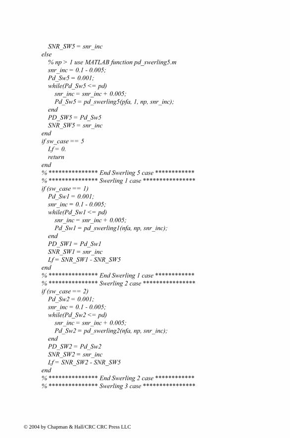
© 200
SNR_SW5 = snr_incelse % np > 1 use MATLAB function pd_swerling5.m snr_inc = 0.1 - 0.005; Pd_Sw5 = 0.001; while(Pd_Sw5 <= pd) snr_inc = snr_inc + 0.005; Pd_Sw5 = pd_swerling5(pfa, 1, np, snr_inc); end PD_SW5 = Pd_Sw5 SNR_SW5 = snr_incendif sw_case == 5 Lf = 0. returnend% *************** End Swerling 5 case ************% *************** Swerling 1 case ****************if (sw_case == 1) Pd_Sw1 = 0.001; snr_inc = 0.1 - 0.005; while(Pd_Sw1 <= pd) snr_inc = snr_inc + 0.005; Pd_Sw1 = pd_swerling1(nfa, np, snr_inc); end PD_SW1 = Pd_Sw1 SNR_SW1 = snr_inc Lf = SNR_SW1 - SNR_SW5end% *************** End Swerling 1 case ************% *************** Swerling 2 case ****************if (sw_case == 2) Pd_Sw2 = 0.001; snr_inc = 0.1 - 0.005; while(Pd_Sw2 <= pd) snr_inc = snr_inc + 0.005; Pd_Sw2 = pd_swerling2(nfa, np, snr_inc); end PD_SW2 = Pd_Sw2 SNR_SW2 = snr_inc Lf = SNR_SW2 - SNR_SW5end% *************** End Swerling 2 case ************% *************** Swerling 3 case ****************
4 by Chapman & Hall/CRC CRC Press LLC
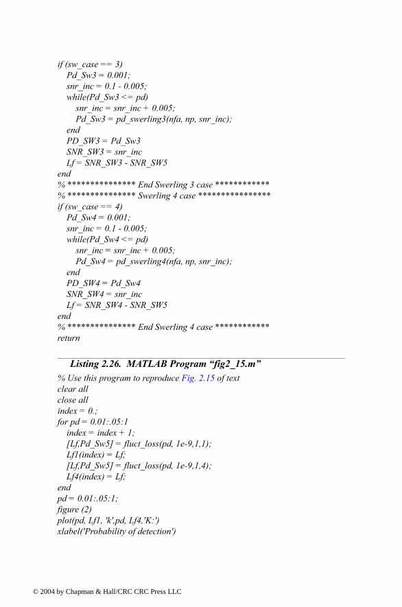
© 200
if (sw_case == 3) Pd_Sw3 = 0.001; snr_inc = 0.1 - 0.005; while(Pd_Sw3 <= pd) snr_inc = snr_inc + 0.005; Pd_Sw3 = pd_swerling3(nfa, np, snr_inc); end PD_SW3 = Pd_Sw3 SNR_SW3 = snr_inc Lf = SNR_SW3 - SNR_SW5end% *************** End Swerling 3 case ************% *************** Swerling 4 case ****************if (sw_case == 4) Pd_Sw4 = 0.001; snr_inc = 0.1 - 0.005; while(Pd_Sw4 <= pd) snr_inc = snr_inc + 0.005; Pd_Sw4 = pd_swerling4(nfa, np, snr_inc); end PD_SW4 = Pd_Sw4 SNR_SW4 = snr_inc Lf = SNR_SW4 - SNR_SW5end% *************** End Swerling 4 case ************return
Listing 2.26. MATLAB Program fig2_15.m% Use this program to reproduce Fig. 2.15 of textclear allclose allindex = 0.;for pd = 0.01:.05:1 index = index + 1; [Lf,Pd_Sw5] = fluct_loss(pd, 1e-9,1,1); Lf1(index) = Lf; [Lf,Pd_Sw5] = fluct_loss(pd, 1e-9,1,4); Lf4(index) = Lf; endpd = 0.01:.05:1;figure (2)plot(pd, Lf1, 'k',pd, Lf4,'K:')xlabel('Probability of detection')
4 by Chapman & Hall/CRC CRC Press LLC
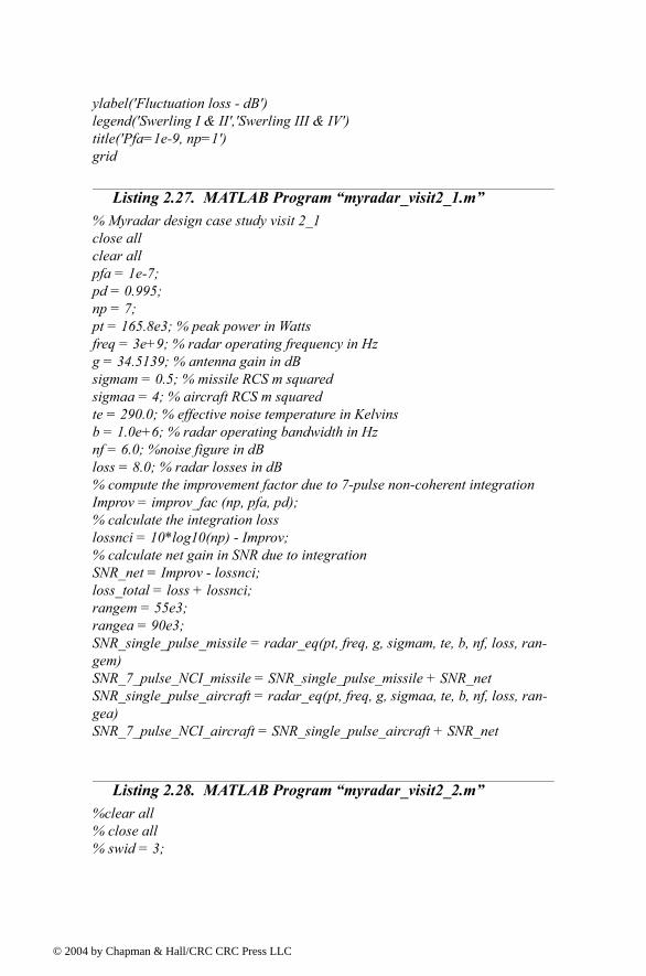
© 200
ylabel('Fluctuation loss - dB')legend('Swerling I & II','Swerling III & IV')title('Pfa=1e-9, np=1')grid
Listing 2.27. MATLAB Program myradar_visit2_1.m% Myradar design case study visit 2_1close allclear allpfa = 1e-7;pd = 0.995;np = 7;pt = 165.8e3; % peak power in Wattsfreq = 3e+9; % radar operating frequency in Hzg = 34.5139; % antenna gain in dBsigmam = 0.5; % missile RCS m squaredsigmaa = 4; % aircraft RCS m squaredte = 290.0; % effective noise temperature in Kelvinsb = 1.0e+6; % radar operating bandwidth in Hznf = 6.0; %noise figure in dBloss = 8.0; % radar losses in dB% compute the improvement factor due to 7-pulse non-coherent integrationImprov = improv_fac (np, pfa, pd);% calculate the integration losslossnci = 10*log10(np) - Improv;% calculate net gain in SNR due to integrationSNR_net = Improv - lossnci;loss_total = loss + lossnci;rangem = 55e3;rangea = 90e3;SNR_single_pulse_missile = radar_eq(pt, freq, g, sigmam, te, b, nf, loss, ran-gem)SNR_7_pulse_NCI_missile = SNR_single_pulse_missile + SNR_net SNR_single_pulse_aircraft = radar_eq(pt, freq, g, sigmaa, te, b, nf, loss, ran-gea)SNR_7_pulse_NCI_aircraft = SNR_single_pulse_aircraft + SNR_net
Listing 2.28. MATLAB Program myradar_visit2_2.m%clear all% close all% swid = 3;
4 by Chapman & Hall/CRC CRC Press LLC
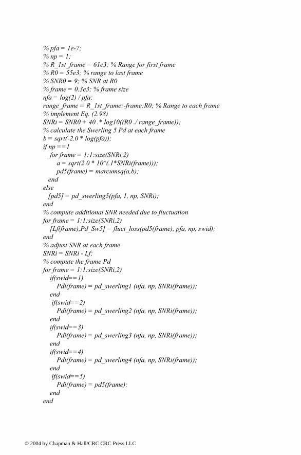
© 200
% pfa = 1e-7;% np = 1;% R_1st_frame = 61e3; % Range for first frame% R0 = 55e3; % range to last frame % SNR0 = 9; % SNR at R0% frame = 0.3e3; % frame sizenfa = log(2) / pfa;range_frame = R_1st_frame:-frame:R0; % Range to each frame% implement Eq. (2.98)SNRi = SNR0 + 40 .* log10((R0 ./ range_frame)); % calculate the Swerling 5 Pd at each frameb = sqrt(-2.0 * log(pfa));if np ==1 for frame = 1:1:size(SNRi,2) a = sqrt(2.0 * 10^(.1*SNRi(frame))); pd5(frame) = marcumsq(a,b); endelse [pd5] = pd_swerling5(pfa, 1, np, SNRi); end% compute additional SNR needed due to fluctuationfor frame = 1:1:size(SNRi,2) [Lf(frame),Pd_Sw5] = fluct_loss(pd5(frame), pfa, np, swid); end% adjust SNR at each frameSNRi = SNRi - Lf;% compute the frame Pdfor frame = 1:1:size(SNRi,2) if(swid==1) Pdi(frame) = pd_swerling1 (nfa, np, SNRi(frame)); end if(swid==2) Pdi(frame) = pd_swerling2 (nfa, np, SNRi(frame)); end if(swid==3) Pdi(frame) = pd_swerling3 (nfa, np, SNRi(frame)); end if(swid==4) Pdi(frame) = pd_swerling4 (nfa, np, SNRi(frame)); end if(swid==5) Pdi(frame) = pd5(frame); endend
4 by Chapman & Hall/CRC CRC Press LLC
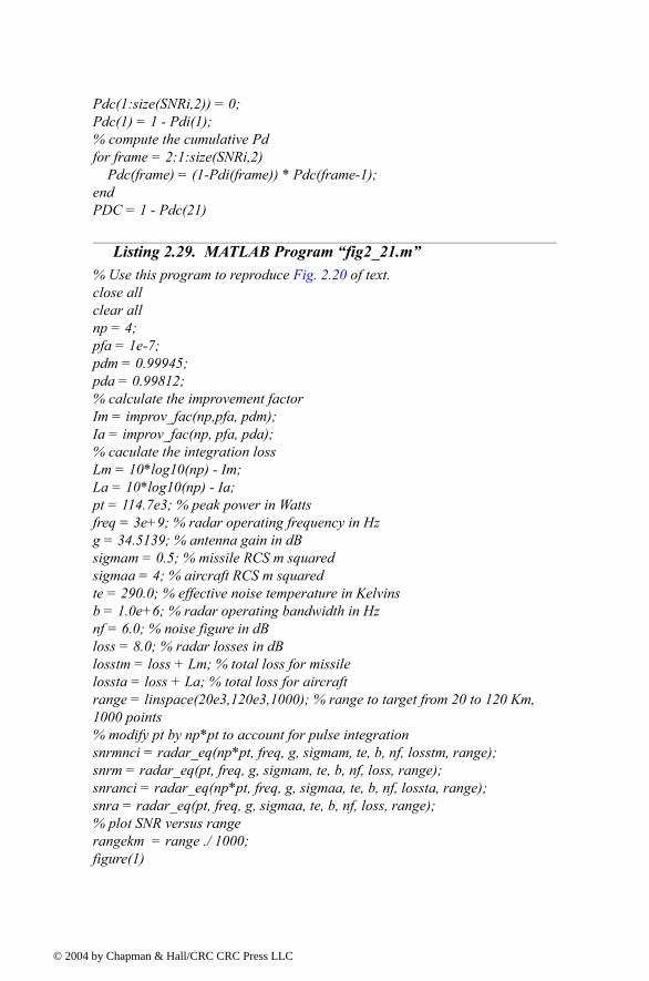
© 200
Pdc(1:size(SNRi,2)) = 0;Pdc(1) = 1 - Pdi(1);% compute the cumulative Pdfor frame = 2:1:size(SNRi,2) Pdc(frame) = (1-Pdi(frame)) * Pdc(frame-1);endPDC = 1 - Pdc(21)
Listing 2.29. MATLAB Program fig2_21.m% Use this program to reproduce Fig. 2.20 of text.close allclear allnp = 4;pfa = 1e-7;pdm = 0.99945;pda = 0.99812;% calculate the improvement factorIm = improv_fac(np,pfa, pdm);Ia = improv_fac(np, pfa, pda);% caculate the integration lossLm = 10*log10(np) - Im;La = 10*log10(np) - Ia;pt = 114.7e3; % peak power in Wattsfreq = 3e+9; % radar operating frequency in Hzg = 34.5139; % antenna gain in dBsigmam = 0.5; % missile RCS m squaredsigmaa = 4; % aircraft RCS m squaredte = 290.0; % effective noise temperature in Kelvinsb = 1.0e+6; % radar operating bandwidth in Hznf = 6.0; % noise figure in dBloss = 8.0; % radar losses in dBlosstm = loss + Lm; % total loss for missilelossta = loss + La; % total loss for aircraftrange = linspace(20e3,120e3,1000); % range to target from 20 to 120 Km, 1000 points% modify pt by np*pt to account for pulse integrationsnrmnci = radar_eq(np*pt, freq, g, sigmam, te, b, nf, losstm, range);snrm = radar_eq(pt, freq, g, sigmam, te, b, nf, loss, range);snranci = radar_eq(np*pt, freq, g, sigmaa, te, b, nf, lossta, range);snra = radar_eq(pt, freq, g, sigmaa, te, b, nf, loss, range);% plot SNR versus rangerangekm = range ./ 1000;figure(1)
4 by Chapman & Hall/CRC CRC Press LLC

© 200
subplot(2,1,1)plot(rangekm,snrmnci,'k',rangekm,snrm,'k -.')gridlegend('With 4-pulse NCI','Single pulse')ylabel ('SNR - dB');title('Missile case')subplot(2,1,2)plot(rangekm,snranci,'k',rangekm,snra,'k -.')gridlegend('With 4-pulse NCI','Single pulse')ylabel ('SNR - dB');title('Aircraft case')xlabel('Detection range - Km')
4 by Chapman & Hall/CRC CRC Press LLC
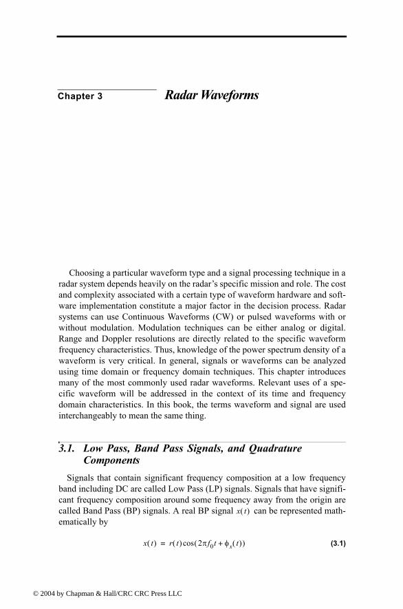
© 200
Chapter 3 Radar Waveforms
Choosing a particular waveform type and a signal processing technique in a radar system depends heavily on the radars specific mission and role. The cost and complexity associated with a certain type of waveform hardware and soft-ware implementation constitute a major factor in the decision process. Radar systems can use Continuous Waveforms (CW) or pulsed waveforms with or without modulation. Modulation techniques can be either analog or digital. Range and Doppler resolutions are directly related to the specific waveform frequency characteristics. Thus, knowledge of the power spectrum density of a waveform is very critical. In general, signals or waveforms can be analyzed using time domain or frequency domain techniques. This chapter introduces many of the most commonly used radar waveforms. Relevant uses of a spe-cific waveform will be addressed in the context of its time and frequency domain characteristics. In this book, the terms waveform and signal are used interchangeably to mean the same thing.
3.1. Low Pass, Band Pass Signals, and Quadrature Components
Signals that contain significant frequency composition at a low frequency band including DC are called Low Pass (LP) signals. Signals that have signifi-cant frequency composition around some frequency away from the origin are called Band Pass (BP) signals. A real BP signal can be represented math-ematically by
(3.1)
x t( )
x t( ) r t( ) 2πf0t φx t( )+( )cos=
4 by Chapman & Hall/CRC CRC Press LLC
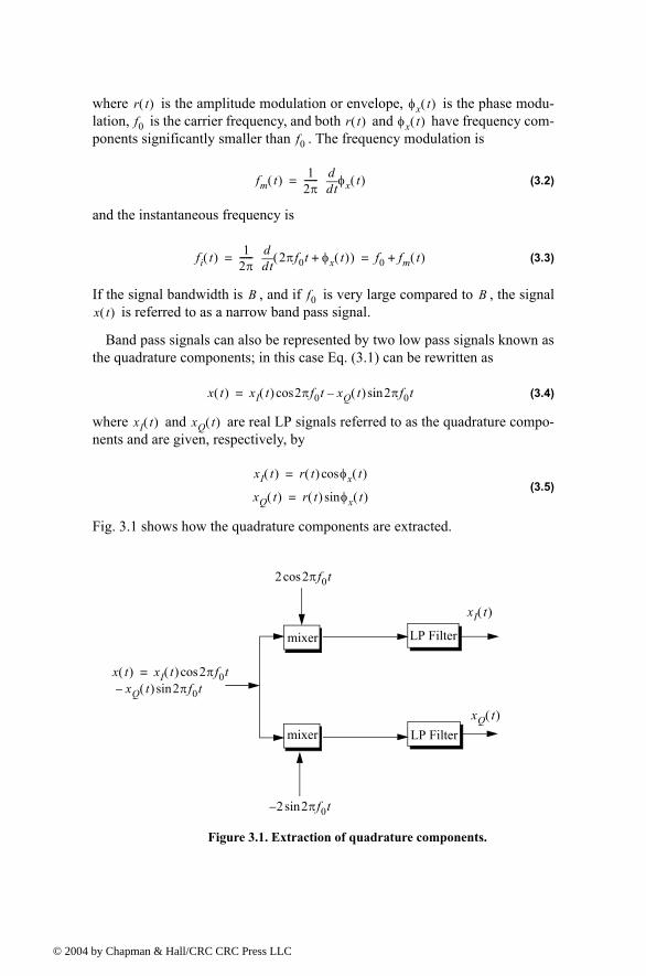
© 200
where is the amplitude modulation or envelope, is the phase modu-lation, is the carrier frequency, and both and have frequency com-ponents significantly smaller than . The frequency modulation is
(3.2)
and the instantaneous frequency is
(3.3)
If the signal bandwidth is , and if is very large compared to , the signal is referred to as a narrow band pass signal.
Band pass signals can also be represented by two low pass signals known as the quadrature components; in this case Eq. (3.1) can be rewritten as
(3.4)
where and are real LP signals referred to as the quadrature compo-nents and are given, respectively, by
(3.5)
Fig. 3.1 shows how the quadrature components are extracted.
r t( ) φx t( )f0 r t( ) φx t( )
f0
fm t( ) 12π------
tdd φx t( )=
fi t( ) 12π------
tdd 2πf0t φx t( )+( ) f0 fm t( )+= =
B f0 Bx t( )
x t( ) xI t( ) 2πf0tcos xQ t( ) 2πf0tsin=
xI t( ) xQ t( )
xI t( ) r t( ) φx t( )cos=
xQ t( ) r t( ) φx t( )sin=
mixer
mixer
LP Filter
LP Filter
2 2πf0tcos
x t( ) xI t( ) 2πf0tcosxQ t( ) 2πf0tsin
=
2 2πf0tsin
xQ t( )
xI t( )
Figure 3.1. Extraction of quadrature components.
4 by Chapman & Hall/CRC CRC Press LLC
© 200
3.2. The Analytic SignalThe sinusoidal signal defined in Eq. (3.1) can be written as the real part
of the complex signal . More precisely,
(3.6)
Define the analytic signal as
(3.7)
where
(3.8)
and
(3.9)
is the Fourier transform of and is the Fourier transform of . Eq. (3.9) can be written as
(3.10)
where is the step function in the frequency domain. Thus, it can be shown that is
(3.11)
is the Hilbert transform of .
Using Eqs. (3.6) and (3.11), one can then write (shown here without proof)
(3.12)
which is similar to Eq. (3.4) with .
Using Parsevals theorem it can be shown that the energy associated with the signal is
(3.13)
x t( )ψ t( )
x t( ) Re ψ t( ) = Re r t( )ejφx t( )
ej2πf0t
=
ψ t( ) v t( )ej2πf0t
=
v t( ) r t( )ejφx t( )
=
Ψ ω( )2X ω( )
0ω 0≥ω 0<
=
Ψ ω( ) ψ t( ) X ω( )x t( )
Ψ ω( ) 2U ω( )X ω( )=
U ω( )ψ t( )
ψ t( ) x t( ) jx t( )+=
x t( ) x t( )
x t( ) u0I t( ) ω0tcos u0Q t( ) ω0tsin=
ω0 2πf0=
x t( )
Ex12--- x2 t( ) td
∞
∞
∫12--- u2 t( ) td
∞
∞
∫12---Eψ= = =
4 by Chapman & Hall/CRC CRC Press LLC
© 200
3.3. CW and Pulsed Waveforms The spectrum of a given signal describes the spread of its energy in the fre-
quency domain. An energy signal (finite energy) can be characterized by its Energy Spectrum Density (ESD) function, while a power signal (finite power) is characterized by the Power Spectrum Density (PSD) function. The units of the ESD are Joules per Hertz and the PSD has units Watts per Hertz.
The signal bandwidth is the range of frequency over which the signal has a nonzero spectrum. In general, any signal can be defined using its duration (time domain) and bandwidth (frequency domain). A signal is said to be band-limited if it has finite bandwidth. Signals that have finite durations (time-lim-ited) will have infinite bandwidths, while band-limited signals have infinite durations. The extreme case is a continuous sine wave, whose bandwidth is infinitesimal.
A time domain signal has a Fourier Transform (FT) given by
(3.14)
where the Inverse Fourier Transform (IFT) is
(3.15)
The signal autocorrelation function is
(3.16)
The asterisk indicates the complex conjugate. The signal amplitude spectrum is . If were an energy signal, then its ESD is ; and if it were a
power signal, then its PSD is which is the FT of the autocorrelation function
(3.17)
First, consider a CW waveform given by
f t( ) F ω( )
F ω( ) f t( )e jωt td∞
∞
∫=
f t( ) 12π------ F ω( )ejωt ωd
∞
∞
∫=
Rf τ( )
Rf τ( ) f∗ t( )f t τ+( ) td∞
∞
∫=
F ω( ) f t( ) F ω( ) 2
Sf ω( )
Sf ω( ) Rf τ( )e jωτ τd∞
∞
∫=
4 by Chapman & Hall/CRC CRC Press LLC
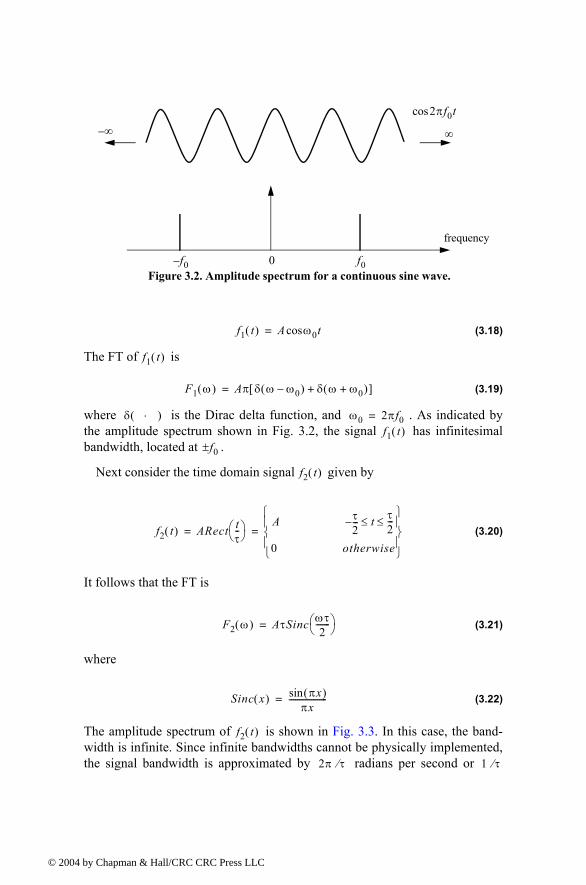
© 200
(3.18)
The FT of is
(3.19)
where is the Dirac delta function, and . As indicated by the amplitude spectrum shown in Fig. 3.2, the signal has infinitesimal bandwidth, located at .
Next consider the time domain signal given by
(3.20)
It follows that the FT is
(3.21)
where
(3.22)
The amplitude spectrum of is shown in Fig. 3.3. In this case, the band-width is infinite. Since infinite bandwidths cannot be physically implemented, the signal bandwidth is approximated by radians per second or
frequency
2πf0tcos
∞∞
f0 f00 Figure 3.2. Amplitude spectrum for a continuous sine wave.
f1 t( ) A ω0tcos=
f1 t( )
F1 ω( ) Aπ δ ω ω0( ) δ ω ω0+( )+[ ]=
δ ⋅( ) ω0 2πf0=f1 t( )
f0±
f2 t( )
f2 t( ) ARect tτ-- A τ
2--- t τ
2---≤ ≤
0 otherwise
= =
F2 ω( ) AτSinc ωτ2
------- =
Sinc x( ) πx( )sinπx
-------------------=
f2 t( )
2π τ⁄ 1 τ⁄
4 by Chapman & Hall/CRC CRC Press LLC
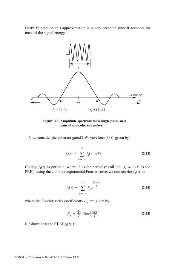
© 200
Hertz. In practice, this approximation is widely accepted since it accounts for most of the signal energy.
Now consider the coherent gated CW waveform given by
(3.23)
Clearly is periodic, where is the period (recall that is the PRF). Using the complex exponential Fourier series we can rewrite as
(3.24)
where the Fourier series coefficients are given by
(3.25)
It follows that the FT of is
frequency
τ
f0 1 τ⁄( ) f0 1 τ⁄( )+
f0
Figure 3.3. Amplitude spectrum for a single pulse, or a train of non-coherent pulses.
∞∞
f3 t( )
f3 t( ) f2 t nT( )
n ∞=
∞
∑=
f3 t( ) T fr 1 T⁄=f3 t( )
f3 t( ) Fnej2πnt
T--------------
n ∞=
∞
∑=
Fn
FnAτT
------ Sinc nτπT
--------- =
f3 t( )
4 by Chapman & Hall/CRC CRC Press LLC
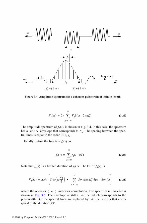
© 200
(3.26)
The amplitude spectrum of is shown in Fig. 3.4. In this case, the spectrum has a envelope that corresponds to . The spacing between the spec-tral lines is equal to the radar PRF, .
Finally, define the function as
(3.27)
Note that is a limited duration of . The FT of is
(3.28)
where the operator indicates convolution. The spectrum in this case is shown in Fig. 3.5. The envelope is still a which corresponds to the pulsewidth. But the spectral lines are replaced by spectra that corre-spond to the duration .
τ
∞∞
frequency
fr
f0 1 τ⁄( ) f0 1 τ⁄( )+
f0
Figure 3.4. Amplitude spectrum for a coherent pulse train of infinite length.
∞∞
F3 ω( ) 2π Fnδ ω 2nπfr( )
n ∞=
∞
∑=
f3 t( )xsin x⁄ Fn
fr
f4 t( )
f4 t( ) f2 t nT( )
n 0=
N
∑=
f4 t( ) f3 t( ) f4 t( )
F4 ω( ) ANτ Sinc ωNT2
------- Sinc nπτfr( )δ ω 2nπfr( )
n ∞=
∞
∑•
=
•( )xsin x⁄
xsin x⁄NT
4 by Chapman & Hall/CRC CRC Press LLC
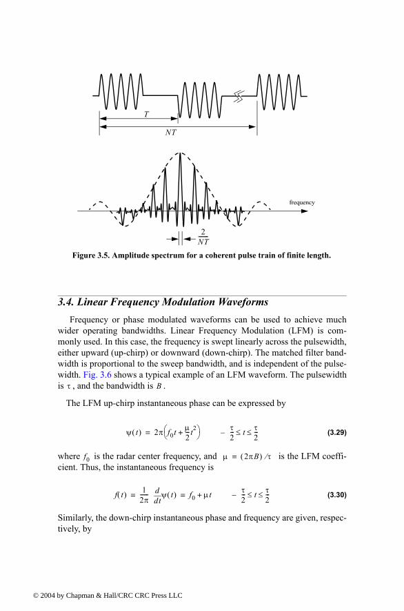
© 200
3.4. Linear Frequency Modulation Waveforms Frequency or phase modulated waveforms can be used to achieve much
wider operating bandwidths. Linear Frequency Modulation (LFM) is com-monly used. In this case, the frequency is swept linearly across the pulsewidth, either upward (up-chirp) or downward (down-chirp). The matched filter band-width is proportional to the sweep bandwidth, and is independent of the pulse-width. Fig. 3.6 shows a typical example of an LFM waveform. The pulsewidth is , and the bandwidth is .
The LFM up-chirp instantaneous phase can be expressed by
(3.29)
where is the radar center frequency, and is the LFM coeffi-cient. Thus, the instantaneous frequency is
(3.30)
Similarly, the down-chirp instantaneous phase and frequency are given, respec-tively, by
Figure 3.5. Amplitude spectrum for a coherent pulse train of finite length.
NT
frequency
2NT-------
T
τ B
ψ t( ) 2π f0t µ2---t2
+ =
τ2--- t τ
2---≤ ≤
f0 µ 2πB( ) τ⁄=
f t( ) 12π------
tdd ψ t( ) f0 µt+= =
τ2--- t τ
2---≤ ≤
4 by Chapman & Hall/CRC CRC Press LLC
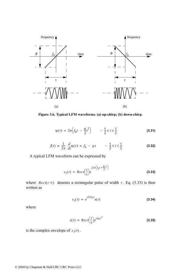
© 200
(3.31)
(3.32)
A typical LFM waveform can be expressed by
(3.33)
where denotes a rectangular pulse of width . Eq. (3.33) is then written as
(3.34)
where
(3.35)
is the complex envelope of .
time
frequency
τ
B f0
(a)
time
frequency
τ
B f0
(b)
Figure 3.6. Typical LFM waveforms. (a) up-chirp; (b) down-chirp.
ψ t( ) 2π f0t µ2---t2
=
τ2--- t τ
2---≤ ≤
f t( ) 12π------
tdd ψ t( ) f0 µt= =
τ2--- t τ
2---≤ ≤
s1 t( ) Rect tτ-- e
j2π f0t µ2--- t2+
=
Rect t τ⁄( ) τ
s1 t( ) ej2πf0t
s t( )=
s t( ) Rect tτ-- ejπµ t2
=
s1 t( )
4 by Chapman & Hall/CRC CRC Press LLC
© 200
The spectrum of the signal is determined from its complex envelope . The complex exponential term in Eq. (3.34) introduces a frequency shift
about the center frequency . Taking the FT of yields
(3.36)
Let , and perform the change of variable
(3.37)
Thus, Eq. (3.36) can be written as
(3.38)
(3.39)
where
(3.40)
(3.41)
The Fresnel integrals, denoted by and , are defined by
(3.42)
(3.43)
s1 t( )s t( )
fo s t( )
S ω( ) Rect tτ-- ejπµt2
e jωt td∞
∞
∫j2πµt2
2----------------- exp e jωt td
τ2---
τ2---
∫= =
µ′ 2πµ 2πB τ⁄= =
x µ′π----- t ω
µ′-----
= dx; µ′π----- dt=
S ω( ) πµ′----- e jω2 2µ′⁄ ejπx2 2⁄ xd
x1
x2
∫=
S ω( ) πµ′----- e jω2 2µ′⁄ ejπx2 2⁄ xd
0
x2
∫ ejπx2 2⁄ xd0
x1
∫
=
x1µ′π----- τ
2--- ω
µ′-----+
Bτ2
------ 1 fB 2⁄----------+
= =
x2µ′π----- τ
2--- ω
µ′-----
Bτ2
------ 1 fB 2⁄----------
= =
C x( ) S x( )
C x( ) πυ2
2--------- cos υd
0
x
∫=
S x( ) πυ2
2--------- sin υd
0
x
∫=
4 by Chapman & Hall/CRC CRC Press LLC
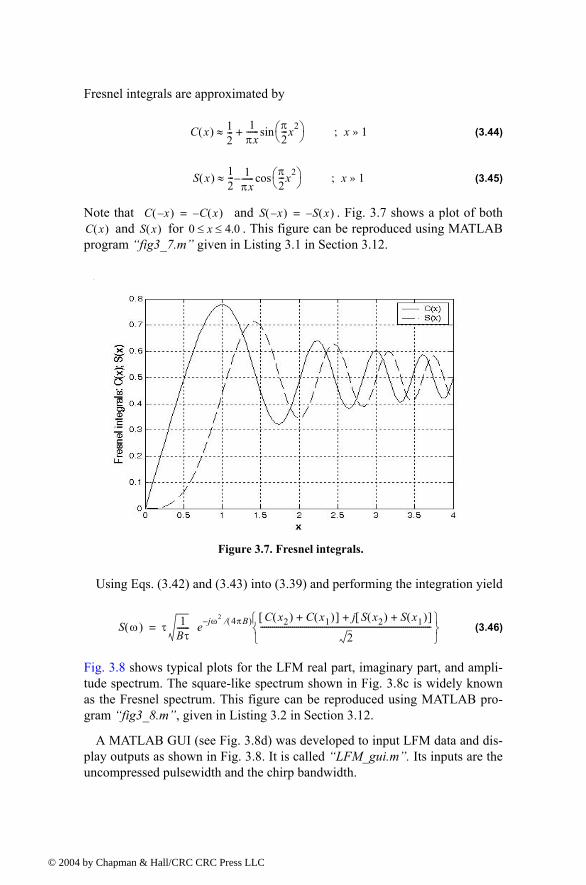
© 200
Fresnel integrals are approximated by
(3.44)
(3.45)
Note that and . Fig. 3.7 shows a plot of both and for . This figure can be reproduced using MATLAB
program fig3_7.m given in Listing 3.1 in Section 3.12.
Using Eqs. (3.42) and (3.43) into (3.39) and performing the integration yield
(3.46)
Fig. 3.8 shows typical plots for the LFM real part, imaginary part, and ampli-tude spectrum. The square-like spectrum shown in Fig. 3.8c is widely known as the Fresnel spectrum. This figure can be reproduced using MATLAB pro-gram fig3_8.m, given in Listing 3.2 in Section 3.12.
A MATLAB GUI (see Fig. 3.8d) was developed to input LFM data and dis-play outputs as shown in Fig. 3.8. It is called LFM_gui.m. Its inputs are the uncompressed pulsewidth and the chirp bandwidth.
C x( ) 12--- 1
πx------ π
2---x2 sin+≈ x 1»;
S x( ) 12--- 1πx------
π2---x2 cos≈ x 1»;
C x( ) C x( )= S x( ) S x( )=C x( ) S x( ) 0 x 4.0≤ ≤
Figure 3.7. Fresnel integrals.
S ω( ) τ 1Bτ------ e jω2 4πB( )⁄ C x2( ) C x1( )+[ ] j S x2( ) S x1( )+[ ]+
2--------------------------------------------------------------------------------------
=
4 by Chapman & Hall/CRC CRC Press LLC
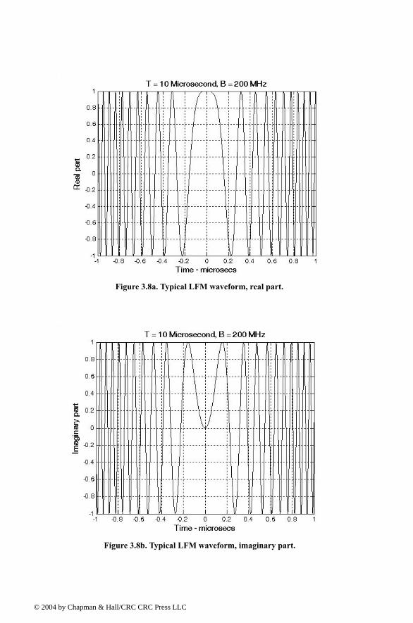
© 2
Figure 3.8a. Typical LFM waveform, real part.
Figure 3.8b. Typical LFM waveform, imaginary part.
004 by Chapman & Hall/CRC CRC Press LLC
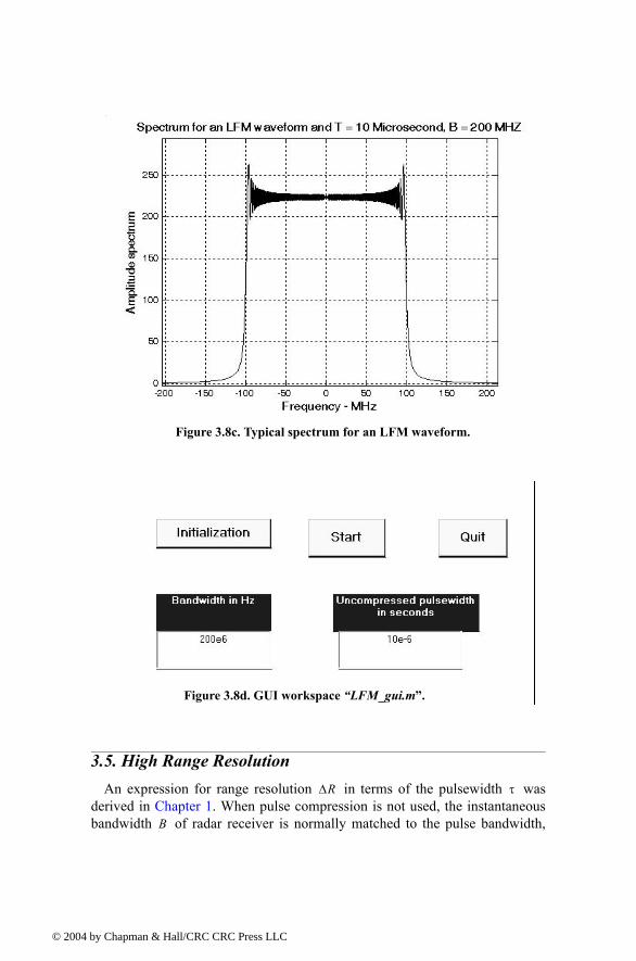
© 200
3.5. High Range Resolution An expression for range resolution in terms of the pulsewidth was
derived in Chapter 1. When pulse compression is not used, the instantaneous bandwidth of radar receiver is normally matched to the pulse bandwidth,
Figure 3.8c. Typical spectrum for an LFM waveform.
Figure 3.8d. GUI workspace LFM_gui.m.
∆R τ
B
4 by Chapman & Hall/CRC CRC Press LLC
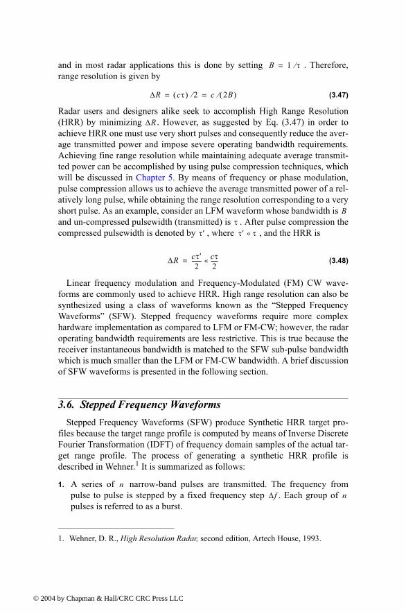
© 200
and in most radar applications this is done by setting . Therefore, range resolution is given by
(3.47)
Radar users and designers alike seek to accomplish High Range Resolution (HRR) by minimizing . However, as suggested by Eq. (3.47) in order to achieve HRR one must use very short pulses and consequently reduce the aver-age transmitted power and impose severe operating bandwidth requirements. Achieving fine range resolution while maintaining adequate average transmit-ted power can be accomplished by using pulse compression techniques, which will be discussed in Chapter 5. By means of frequency or phase modulation, pulse compression allows us to achieve the average transmitted power of a rel-atively long pulse, while obtaining the range resolution corresponding to a very short pulse. As an example, consider an LFM waveform whose bandwidth is and un-compressed pulsewidth (transmitted) is . After pulse compression the compressed pulsewidth is denoted by , where , and the HRR is
(3.48)
Linear frequency modulation and Frequency-Modulated (FM) CW wave-forms are commonly used to achieve HRR. High range resolution can also be synthesized using a class of waveforms known as the Stepped Frequency Waveforms (SFW). Stepped frequency waveforms require more complex hardware implementation as compared to LFM or FM-CW; however, the radar operating bandwidth requirements are less restrictive. This is true because the receiver instantaneous bandwidth is matched to the SFW sub-pulse bandwidth which is much smaller than the LFM or FM-CW bandwidth. A brief discussion of SFW waveforms is presented in the following section.
3.6. Stepped Frequency Waveforms Stepped Frequency Waveforms (SFW) produce Synthetic HRR target pro-
files because the target range profile is computed by means of Inverse Discrete Fourier Transformation (IDFT) of frequency domain samples of the actual tar-get range profile. The process of generating a synthetic HRR profile is described in Wehner.1 It is summarized as follows:
1. A series of narrow-band pulses are transmitted. The frequency from pulse to pulse is stepped by a fixed frequency step . Each group of pulses is referred to as a burst.
1. Wehner, D. R., High Resolution Radar, second edition, Artech House, 1993.
B 1 τ⁄=
∆R cτ( ) 2⁄ c 2B( )⁄= =
∆R
Bτ
τ′ τ′ τ«
∆R cτ′2
------- cτ2-----«=
n∆f n
4 by Chapman & Hall/CRC CRC Press LLC
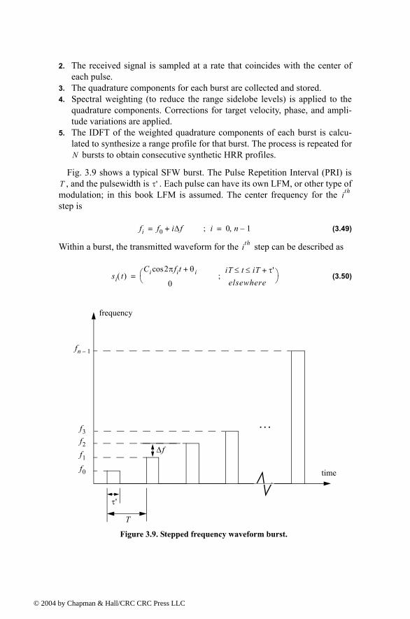
© 200
2. The received signal is sampled at a rate that coincides with the center of each pulse.
3. The quadrature components for each burst are collected and stored.4. Spectral weighting (to reduce the range sidelobe levels) is applied to the
quadrature components. Corrections for target velocity, phase, and ampli-tude variations are applied.
5. The IDFT of the weighted quadrature components of each burst is calcu-lated to synthesize a range profile for that burst. The process is repeated for
bursts to obtain consecutive synthetic HRR profiles.
Fig. 3.9 shows a typical SFW burst. The Pulse Repetition Interval (PRI) is , and the pulsewidth is . Each pulse can have its own LFM, or other type of
modulation; in this book LFM is assumed. The center frequency for the step is
(3.49)
Within a burst, the transmitted waveform for the step can be described as
(3.50)
N
T τ'ith
fi f0 i∆f+= i; 0 n 1,=
ith
si t( )Ci 2πfit θi+cos
0=
iT t iT τ'+≤ ≤elsewhere
;
…
f0
f1
f2
f3
fn 1
∆f
τ'
T
time
frequency
Figure 3.9. Stepped frequency waveform burst.
4 by Chapman & Hall/CRC CRC Press LLC
© 200
where are the relative phases and are constants. The received signal from a target located at range at time is then given by
(3.51)
where are constant and the round trip delay is given by
(3.52)
is the speed of light and is the target radial velocity.
The received signal is down-converted to base-band in order to extract the quadrature components. More precisely, is mixed with the signal
(3.53)
After low pass filtering, the quadrature components are given by
(3.54)
where are constants, and
(3.55)
where now . For each pulse, the quadrature components are then sam-pled at
(3.56)
is the time delay associated with the range that corresponds to the start of the range profile.
The quadrature components can then be expressed in complex form as
(3.57)
Eq. (3.57) represents samples of the target reflectivity, due to a single burst, in the frequency domain. This information can then be transformed into a series of range delay reflectivity (i.e., range profile) values by using the IDFT. It fol-lows that
θi CiR0 t 0=
sri t( ) Ci′ 2πfi t τ t( )( ) θi+( )cos= iT τ t( )+ t iT τ' τ t( )+ +≤ ≤;
Ci′ τ t( )
τ t( )R0 vt
c 2⁄----------------=
c v
sri t( )
yi t( ) C 2πfit θi+( )cos= iT t iT τ'+≤ ≤;
xI t( )
xQ t( ) Ai ψi t( )cos
Ai ψi t( )sin
=
Ai
ψi t( ) 2πfi2R0
c--------- 2vt
c--------
=
fi ∆f=
ti iTτr2----
2R0c
---------+ +=
τr
Xi Aiejψi=
4 by Chapman & Hall/CRC CRC Press LLC
© 200
(3.58)
Substituting Eqs. (3.57) and (3.55) into (3.58) and collecting terms yield
(3.59)
By normalizing with respect to and by assuming that and that the target is stationary (i.e., ), then Eq. (3.59) can be written as
(3.60)
Using inside Eq. (3.60) yields
(3.61)
which can be simplified to
(3.62)
where
(3.63)
Finally, the synthesized range profile is
(3.64)
3.6.1. Range Resolution and Range Ambiguity in SFW
As usual, range resolution is determined from the overall system bandwidth. Assuming a SFW with steps, and step size , then the corresponding range resolution is equal to
Hl1n--- Xi j2πli
n----------
expi 0=
n 1
∑= 0 l n 1≤ ≤;
Hl1n--- Ai j 2πli
n---------- 2πfi
2R0c
---------2vti
c---------
expi 0=
n 1
∑=
n Ai 1=v 0=
Hl j 2πlin
---------- 2πfi2R0
c---------
expi 0=
n 1
∑=
fi i∆f=
Hl j2πin
--------2nR0∆f
c------------------- l+
expi 0=
n 1
∑=
Hlπχsinπχn
------sin--------------- jn 1
2------------ 2πχ
n----------
exp=
χ2nR0∆f
c---------------------- l+=
Hlπχsinπχn
------sin---------------=
n ∆f
4 by Chapman & Hall/CRC CRC Press LLC
© 200
(3.65)
Range ambiguity associated with a SFW can be determined by examining the phase term that corresponds to a point scatterer located at range . More precisely,
(3.66)
It follows that
(3.67)
or equivalently,
(3.68)
It is clear from Eq. (3.68) that range ambiguity exists for . Therefore,
(3.69)
and the unambiguous range window is
(3.70)
Hence, a range profile synthesized using a particular SFW represents the rel-ative range reflectivity for all scatterers within the unambiguous range win-dow, with respect to the absolute range that corresponds to the burst time delay. Additionally, if a specific target extent is larger than , then all scatterers fall-ing outside the unambiguous range window will fold over and appear in the synthesized profile. This fold-over problem is identical to the spectral fold-over that occurs when using a Fast Fourier Transform (FFT) to resolve certain signal frequency contents. For example, consider an FFT with frequency reso-lution , and size . In this case, this FFT can resolve frequency tones between and . When this FFT is used to resolve the frequency content of a sine-wave tone equal to , fold-over occurs and a spectral line at the fourth FFT bin (i.e., ) appears. There-fore, in order to avoid fold-over in the synthesized range profile, the frequency step must be
∆R c2n∆f------------=
R0
ψi t( ) 2πfi2R0
c---------=
∆ψ∆f--------
4π fi 1+ fi( )fi 1+ fi( )
-------------------------------R0c
------4πR0
c-------------= =
R0∆ψ∆f-------- c
4π------=
∆ψ ∆ψ 2nπ+=
R0∆ψ 2nπ+
∆f------------------------ c
4π------ R0 n c
2∆f--------- += =
Ruc
2∆f---------=
Ru
∆f 50Hz= NFFT 64=1600Hz 1600Hz
1800Hz200Hz
∆f
4 by Chapman & Hall/CRC CRC Press LLC
Stepped Frequency Waveforms 159
© 200
(3.71)
where is the target extent in meters.
Additionally, the pulsewidth must also be large enough to contain the whole target extent. Thus,
(3.72)
and, in practice, (3.73)
This is necessary in order to reduce the amount of contamination of the synthe-sized range profile caused by the clutter surrounding the target under consider-ation.
MATLAB Function hrr_profile.m
The function hrr_profile.m computes and plots the synthetic HRR profile for a specific SFW. It is given in Listing 3.3 in Section 3.12. This function uti-lizes an Inverse Fast Fourier Transform (IFFT) of a size equal to twice the number of steps. Hamming window of the same size is also assumed. The syn-tax is as follows:
[hl] = hrr_profile (nscat, scat_range, scat_rcs, n, deltaf, prf, v, r0, winid)
where
Symbol Description Units Status
nscat number of scatterers that make up the target
none input
scat_range vector containing range to individ-ual scatterers
meters input
scat_rcs vector containing RCS of individual scatterers
meter square input
n number of steps none input
deltaf frequency step Hz input
prf PRF of SFW Hz input
v target velocity meter/second input
r0 profile starting range meters input
winid number>0 for Hamming window
number < 0 for no window
none input
hl range profile dB output
∆f c 2E⁄≤
E
∆f 1 τ'⁄≤
∆f 1 2τ'⁄≤
4 by Chapman & Hall/CRC CRC Press LLC
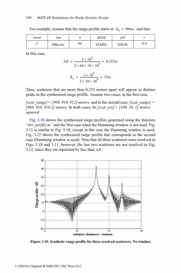
160 MATLAB Simulations for Radar Systems Design
© 200
For example, assume that the range profile starts at and that
In this case,
Thus, scatterers that are more than 0.235 meters apart will appear as distinct peaks in the synthesized range profile. Assume two cases; in the first case,
[scat_range] = [908, 910, 912] meters, and in the second case, [scat_range] = [908, 910, 910.2] meters. In both cases, let [scat_rcs] = [100, 10, 1] meters squared.
Fig. 3.10 shows the synthesized range profiles generated using the function hrr_profile.m and the first case when the Hamming window is not used. Fig. 3.11 is similar to Fig. 3.10, except in this case the Hamming window is used. Fig. 3.12 shows the synthesized range profile that corresponds to the second case (Hamming window is used). Note that all three scatterers were resolved in Figs. 3.10 and 3.11; however, the last two scatterers are not resolved in Fig. 3.12, since they are separated by less than .
nscat tau n deltaf prf v
3 64 0.0
R0 900m=
100µ sec 10MHz 10KHz
∆R 3 108×
2 64× 10 106××------------------------------------------ 0.235m= =
Ru3 108×
2 10 106××------------------------------ 15m= =
∆R
Figure 3.10. Synthetic range profile for three resolved scatterers. No window.
4 by Chapman & Hall/CRC CRC Press LLC
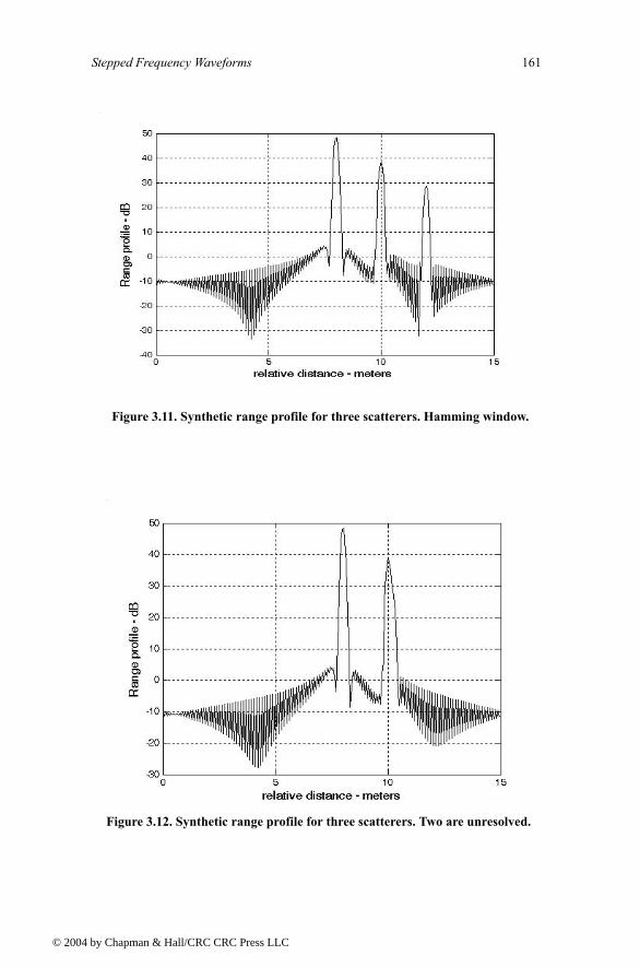
Stepped Frequency Waveforms 161
© 200
Figure 3.11. Synthetic range profile for three scatterers. Hamming window.
Figure 3.12. Synthetic range profile for three scatterers. Two are unresolved.
4 by Chapman & Hall/CRC CRC Press LLC
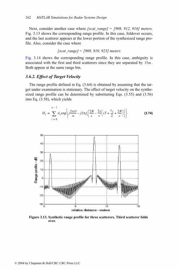
162 MATLAB Simulations for Radar Systems Design
© 200
Next, consider another case where [scat_range] = [908, 912, 916] meters. Fig. 3.13 shows the corresponding range profile. In this case, foldover occurs, and the last scatterer appears at the lower portion of the synthesized range pro-file. Also, consider the case where
[scat_range] = [908, 910, 923] meters
Fig. 3.14 shows the corresponding range profile. In this case, ambiguity is associated with the first and third scatterers since they are separated by . Both appear at the same range bin.
3.6.2. Effect of Target Velocity
The range profile defined in Eq. (3.64) is obtained by assuming that the tar-get under examination is stationary. The effect of target velocity on the synthe-sized range profile can be determined by substituting Eqs. (3.55) and (3.56) into Eq. (3.58), which yields
(3.74)
15m
Hl Ai j2πlin
---------- j2πfi2Rc
------- 2vc
------ iTτ12----- 2R
c-------+ +
expi 0=
n 1
∑=
Figure 3.13. Synthetic range profile for three scatterers. Third scatterer folds over.
4 by Chapman & Hall/CRC CRC Press LLC
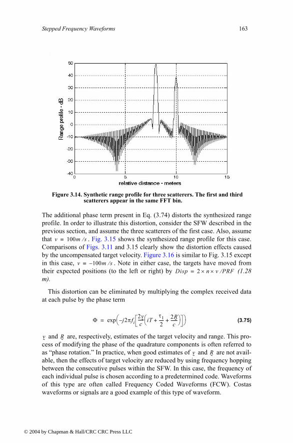
Stepped Frequency Waveforms 163
© 200
The additional phase term present in Eq. (3.74) distorts the synthesized range profile. In order to illustrate this distortion, consider the SFW described in the previous section, and assume the three scatterers of the first case. Also, assume that . Fig. 3.15 shows the synthesized range profile for this case. Comparisons of Figs. 3.11 and 3.15 clearly show the distortion effects caused by the uncompensated target velocity. Figure 3.16 is similar to Fig. 3.15 except in this case, . Note in either case, the targets have moved from their expected positions (to the left or right) by (1.28 m).
This distortion can be eliminated by multiplying the complex received data at each pulse by the phase term
(3.75)
and are, respectively, estimates of the target velocity and range. This pro-cess of modifying the phase of the quadrature components is often referred to as phase rotation. In practice, when good estimates of and are not avail-able, then the effects of target velocity are reduced by using frequency hopping between the consecutive pulses within the SFW. In this case, the frequency of each individual pulse is chosen according to a predetermined code. Waveforms of this type are often called Frequency Coded Waveforms (FCW). Costas waveforms or signals are a good example of this type of waveform.
Figure 3.14. Synthetic range profile for three scatterers. The first and third scatterers appear in the same FFT bin.
v 100m s⁄=
v 100 m s⁄=Disp 2 n v×× PRF⁄=
Φ j 2πfi2v
c------ iT
τ12----- 2R
c-------+ +
exp=
v
R
v
R
4 by Chapman & Hall/CRC CRC Press LLC
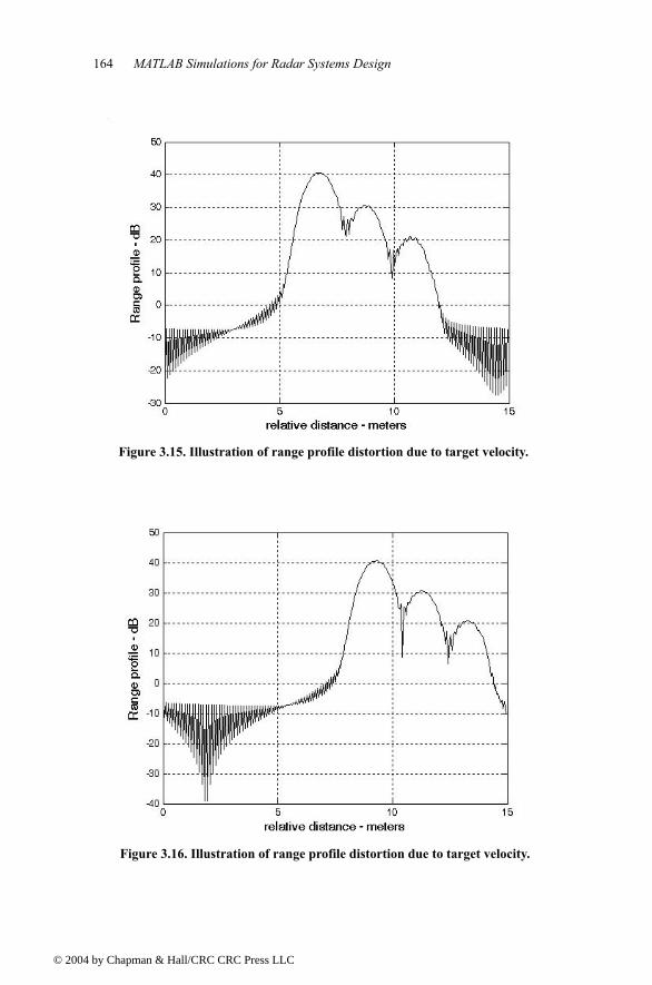
164 MATLAB Simulations for Radar Systems Design
© 200
Figure 3.15. Illustration of range profile distortion due to target velocity.
Figure 3.16. Illustration of range profile distortion due to target velocity.
4 by Chapman & Hall/CRC CRC Press LLC
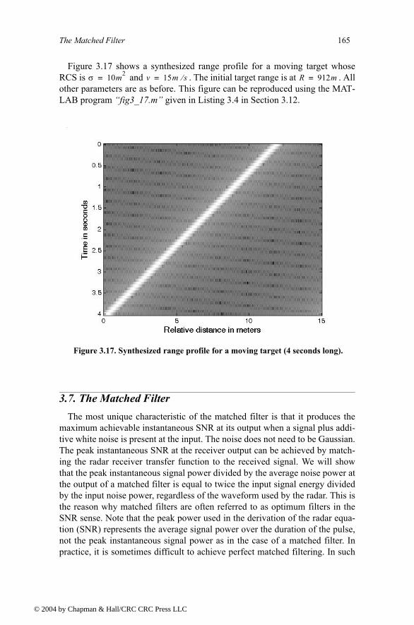
The Matched Filter 165
© 200
Figure 3.17 shows a synthesized range profile for a moving target whose RCS is and . The initial target range is at . All other parameters are as before. This figure can be reproduced using the MAT-LAB program fig3_17.m given in Listing 3.4 in Section 3.12.
3.7. The Matched FilterThe most unique characteristic of the matched filter is that it produces the
maximum achievable instantaneous SNR at its output when a signal plus addi-tive white noise is present at the input. The noise does not need to be Gaussian. The peak instantaneous SNR at the receiver output can be achieved by match-ing the radar receiver transfer function to the received signal. We will show that the peak instantaneous signal power divided by the average noise power at the output of a matched filter is equal to twice the input signal energy divided by the input noise power, regardless of the waveform used by the radar. This is the reason why matched filters are often referred to as optimum filters in the SNR sense. Note that the peak power used in the derivation of the radar equa-tion (SNR) represents the average signal power over the duration of the pulse, not the peak instantaneous signal power as in the case of a matched filter. In practice, it is sometimes difficult to achieve perfect matched filtering. In such
σ 10m2= v 15m s⁄= R 912m=
Figure 3.17. Synthesized range profile for a moving target (4 seconds long).
4 by Chapman & Hall/CRC CRC Press LLC
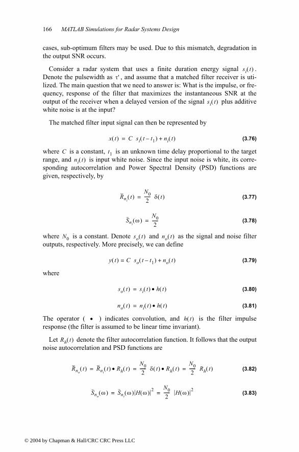
166 MATLAB Simulations for Radar Systems Design
© 200
cases, sub-optimum filters may be used. Due to this mismatch, degradation in the output SNR occurs.
Consider a radar system that uses a finite duration energy signal . Denote the pulsewidth as , and assume that a matched filter receiver is uti-lized. The main question that we need to answer is: What is the impulse, or fre-quency, response of the filter that maximizes the instantaneous SNR at the output of the receiver when a delayed version of the signal plus additive white noise is at the input?
The matched filter input signal can then be represented by
(3.76)
where is a constant, is an unknown time delay proportional to the target range, and is input white noise. Since the input noise is white, its corre-sponding autocorrelation and Power Spectral Density (PSD) functions are given, respectively, by
(3.77)
(3.78)
where is a constant. Denote and as the signal and noise filter outputs, respectively. More precisely, we can define
(3.79)
where
(3.80)
(3.81)
The operator ( ) indicates convolution, and is the filter impulse response (the filter is assumed to be linear time invariant).
Let denote the filter autocorrelation function. It follows that the output noise autocorrelation and PSD functions are
(3.82)
(3.83)
si t( )τ'
si t( )
x t( ) C si t t1( ) ni t( )+=
C t1ni t( )
Rnit( )
N02
------ δ t( )=
Sniω( )
N02
------=
N0 so t( ) no t( )
y t( ) C so t t1( )= no t( )+
so t( ) si t( ) h t( )•=
no t( ) ni t( ) h t( )•=
• h t( )
Rh t( )
Rnot( ) Rni
t( ) Rh t( )•N02
------ δ t( ) Rh t( )•N02
------ Rh t( )= = =
Snoω( ) Sni
ω( ) H ω( ) 2 N02
------ H ω( ) 2= =
4 by Chapman & Hall/CRC CRC Press LLC
The Matched Filter 167
© 200
where is the Fourier transform for the filter impulse response, . The total average output noise power is equal to evaluated at . More precisely,
(3.84)
The output signal power evaluated at time is , and by using Eq. (3.80) we get
(3.85)
A general expression for the output SNR at time can be written as
(3.86)
Substituting Eqs. (3.84) and (3.85) into Eq. (3.86) yields
(3.87)
The Schwartz inequality states that
(3.88)
where the equality applies only when , where is a constant and can be assumed to be unity. Then by applying Eq. (3.88) on the numerator of Eq. (3.87), we get
(3.89)
H ω( ) h t( )Rno
t( ) t 0=
Rno0( )
N02
------ h u( ) 2 ud∞
∞
∫=
t Cso t t1( ) 2
so t t1( ) si t t1 u( ) h u( ) ud∞
∞
∫=
t
SNR t( )Cso t t1( ) 2
Rno0( )
-------------------------------=
SNR t( )
C2 si t t1 u( ) h u( ) ud∞
∞
∫2
N02
------ h u( ) 2 ud∞
∞
∫
-------------------------------------------------------------------------=
P x( )Q x( ) xd∞
∞
∫2
P x( ) 2 xd∞
∞
∫ Q x( ) 2 xd∞
∞
∫≤
P kQ∗= k
SNR t( )
C2 si t t1 u( ) 2 ud∞
∞
∫ h u( ) 2 ud∞
∞
∫
N02
------ h u( ) 2 ud∞
∞
∫
-----------------------------------------------------------------------------------------------≤
2C2 si t t1 u( ) 2 ud∞
∞
∫N0
-------------------------------------------------------------=
4 by Chapman & Hall/CRC CRC Press LLC
168 MATLAB Simulations for Radar Systems Design
© 200
Eq. (3.89) tells us that the peak instantaneous SNR occurs when equality is achieved (i.e., from Eq. (3.88) ). More precisely, if we assume that equality occurs at , and that , then
(3.90)
and the maximum instantaneous SNR is
(3.91)
Eq. (3.91) can be simplified using Parsevals theorem,
(3.92)
where denotes the energy of the input signal; consequently we can write the output peak instantaneous SNR as
(3.93)
Thus, we can draw the conclusion that the peak instantaneous SNR depends only on the signal energy and input noise power, and is independent of the waveform utilized by the radar.
Finally, we can define the impulse response for the matched filter from Eq. (3.90). If we desire the peak to occur at , we get the non-causal matched filter impulse response,
(3.94)
Alternatively, the causal impulse response is
(3.95)
where, in this case, the peak occurs at . It follows that the Fourier transforms of and are given, respectively, by
(3.96)
(3.97)
h ksi∗=t t0= k 1=
h u( ) si∗ t0 t1 u( )=
SNR t0( )
2C2 si t0 t1 u( ) 2 ud∞
∞
∫N0
----------------------------------------------------------------=
E C2 si t0 t1 u( ) 2 ud∞
∞
∫=
E
SNR t0( ) 2EN0-------=
t0 t1=
hnc t( ) si∗ t( )=
hc t( ) si∗ τ t( )=
t0 t1 τ+=hnc t( ) hc t( )
Hnc ω( ) Si∗ ω( )=
Hc ω( ) Si∗ ω( )e jωτ=
4 by Chapman & Hall/CRC CRC Press LLC
The Replica 169
© 200
where is the Fourier transform of . Thus, the moduli of and are identical; however, the phase responses are opposite of each other.
Example:
Compute the maximum instantaneous SNR at the output of a linear filter whose impulse response is matched to the signal .
Solution:
The signal energy is
It follows that the maximum instantaneous SNR is
where is the input noise power spectrum density.
3.8. The ReplicaAgain, consider a radar system that uses a finite duration energy signal ,
and assume that a matched filter receiver is utilized. The input signal is given in Eq. (3.76) and is repeated here as Eq. (3.98),
(3.98)
The matched filter output can be expressed by the convolution integral between the filters impulse response and ,
(3.99)
Substituting Eq. (3.95) into Eq. (3.99) yields
(3.100)
where is a cross-correlation between and . Therefore, the matched filter output can be computed from the cross-correlation between the radar received signal and a delayed replica of the transmitted waveform. If the input signal is the same as the transmitted signal, the output of the matched
Si ω( ) si t( ) H ω( )Si ω( )
x t( ) t2 2T⁄( )exp=
E x t( ) 2 td∞
∞
∫ e t2( ) T⁄ td∞
∞
∫ πT Joules= = =
SNR πTN0 2⁄-------------=
N0 2⁄
si t( )
x t( ) C si t t1( ) ni t( )+=
y t( )x t( )
y t( ) x u( )h t u( ) ud∞
∞
∫=
y t( ) x u( )si∗ τ t u+( ) ud∞
∞
∫ Rxsit τ( )= =
Rxsit τ( ) x t( ) si τ t( )
4 by Chapman & Hall/CRC CRC Press LLC
170 MATLAB Simulations for Radar Systems Design
© 200
filter would be the autocorrelation function of the received (or transmitted) sig-nal. In practice, replicas of the transmitted waveforms are normally computed and stored in memory for use by the radar signal processor when needed.
3.9. Matched Filter Response to LFM WaveformsIn order to develop a general expression for the matched filter output when
an LFM waveform is utilized, we will consider the case when the radar is tracking a closing target with velocity . The transmitted signal is
(3.101)
The received signal is then given by
(3.102)
(3.103)
where is the time corresponding to the target initial detection range, and is the speed of light. Using Eq. (3.103) we can rewrite Eq. (3.102) as
(3.104)
and
(3.105)
is the scaling coefficient. Substituting Eq. (3.101) into Eq. (3.104) yields
(3.106)
which is the analytical signal representation for . The complex envelope of the signal is obtained by multiplying Eq. (3.106) by . Denote the complex envelope by ; then after some manipulation we get
(3.107)
The Doppler shift due to the target motion is
v
s1 t( ) Rect tτ'--- e
j2π f0t µ2--- t2
+
=
sr1t( ) s1 t ∆ t( )( )=
∆ t( ) t02vc
------ t t0( )=
t0 c
sr1t( ) s1 t t0
2vc
------ t t0( )+ s1 γ t t0( )( )= =
γ 1 2vc--+=
sr1t( ) Rect
γ t t0( )τ'
------------------- e
j2πf0γ t t0( )e
jπµγ2 t t0( )2
=
sr1t( )
sr1t( ) j2πf0t( )exp
sr t( )
sr t( ) ej2πf0t0
Rectγ t t0( )
τ'------------------- e
j2πf0 γ 1( ) t t0( )e
jπµγ2 t t0( )2
=
4 by Chapman & Hall/CRC CRC Press LLC
Matched Filter Response to LFM Waveforms 171
© 200
(3.108)
and since , we get
(3.109)
Using the approximation and Eq. (3.109), Eq. (3.107) is rewritten as
(3.110)
where
(3.111)
is given in Eq. (3.101). The matched filter response is given by the con-volution integral
(3.112)
For a non-causal matched filter the impulse response is equal to ; it follows that
(3.113)
Substituting Eq. (3.111) into Eq. (3.113), and performing some algebraic manipulations, we get
(3.114)
Finally, making the change of variable yields
(3.115)
It is customary to set . It follows that
(3.116)
fd2vc
------f0=
γ 1 2v c⁄=
fd γ 1( )f0=
γ 1≈
sr t( ) ej2πfd t t0( )
s t t0( )≈
s t t0( ) ej2πf0t
s1 t t0( )=
s1 t( )
so t( ) h u( )sr t u( )
∞
∞
∫ du=
h u( ) s∗ t( )
so t( ) s∗ u( )sr t u( ) ud∞
∞
∫=
so t( ) s∗ u( ) ej2πfd t u t0+( )
s t u t0+( ) ud∞
∞
∫=
t' t u+=
so t( ) s∗ t' t( )s t' t0( )ej2πfd t' t0( )
t'd∞
∞
∫=
t0 0=
so t fd;( ) s t'( )s∗ t' t( )ej2πfdt'
t'd∞
∞
∫=
4 by Chapman & Hall/CRC CRC Press LLC
172 MATLAB Simulations for Radar Systems Design
© 200
where we used the notation to indicate that the output is a function of both time and Doppler frequency.
3.10. Waveform Resolution and AmbiguityAs indicated by Eq. (3.93) the radar sensitivity (in the case of white additive
noise) depends only on the total energy of the received signal and is indepen-dent of the shape of the specific waveform. This leads us to ask the following question: If the radar sensitivity is independent of the waveform, then what is the best choice for a transmitted waveform? The answer depends on many fac-tors; however, the most important consideration lies in the waveforms range and Doppler resolution characteristics.
As discussed in Chapter 1, range resolution implies separation between dis-tinct targets in range. Alternatively, Doppler resolution implies separation between distinct targets in frequency. Thus, ambiguity and accuracy of this separation are closely associated terms.
3.10.1. Range Resolution
Consider radar returns from two stationary targets (zero Doppler) separated in range by distance . What is the smallest value of so that the returned signal is interpreted by the radar as two distinct targets? In order to answer this question, assume that the radar transmitted pulse is denoted by ,
(3.117)
where is the carrier frequency, is the amplitude modulation, and is the phase modulation. The signal can then be expressed as the real part of the complex signal , where
(3.118)
and
(3.119)
It follows that
(3.120)
The returns from both targets are respectively given by
(3.121)
(3.122)
so t fd;( )
∆R ∆R
s t( )
s t( ) A t( ) 2πf0t φ t( )+( )cos=
f0 A t( ) φ t( )s t( )
ψ t( )
ψ t( ) A t( )ej ω0t φ t( )( )
u t( )ejω0t
= =
u t( ) A t( )e jφ t( )=
s t( ) Re ψ t( ) =
sr1 t( ) ψ t τ0( )=
sr2 t( ) ψ t τ0 τ( )=
4 by Chapman & Hall/CRC CRC Press LLC
Waveform Resolution and Ambiguity 173
© 200
where is the difference in delay between the two returns. One can assume that the reference time is , and thus without any loss of generality one may set . It follows that the two targets are distinguishable by how large or small the delay can be.
In order to measure the difference in range between the two targets consider the integral square error between and . Denoting this error as , it follows that
(3.123)
Eq. (3.123) can be written as
(3.124)
Using Eq. (3.118) into Eq. (3.124) yields
(3.125)
The first term in the right hand side of Eq. (3.125) represents the signal energy, and is assumed to be constant. The second term is a varying function of with its fluctuation tied to the carrier frequency. The integral inside the right-most side of this equation is defined as the range ambiguity function,
(3.126)
The maximum value of is at . Target resolvability in range is measured by the squared magnitude . It follows that if
for some nonzero value of , then the two targets are indistin-guishable. Alternatively, if for some nonzero value of , then the two targets may be distinguishable (resolvable). As a consequence, the most desirable shape for is a very sharp peak (thumb tack shape) cen-tered at and falling very quickly away from the peak.
ττ0
τ0 0=τ
ψ t( ) ψ t τ( ) εR2
εR2 ψ t( ) ψ t τ( )
2 td∞
∞
∫=
εR2 ψ t( ) 2 td
∞
∞
∫ ψ t τ( ) 2 td∞
∞
∫
ψ t( )ψ∗ t τ( ) ψ∗ t( )ψ t τ( )+( ) td
∞
∞
∫
+=
εR2 2 u t( ) 2 td
∞
∞
∫ 2Re ψ∗ t( )ψ t τ( ) td∞
∞
∫
2 u t( ) 2 td∞
∫ 2Re ejω0τ
u∗ t( )u t τ( ) td∞
∫
= =
τ
χR τ( ) u∗ t( )u t τ( ) td∞
∞
∫=
χR τ( ) τ 0=χR τ( ) 2
χR τ( ) χR 0( )= τχR τ( ) χR 0( )≠ τ
χR τ( )τ 0=
4 by Chapman & Hall/CRC CRC Press LLC
174 MATLAB Simulations for Radar Systems Design
© 200
The time delay resolution is
(3.127)
Using Parsevals theorem, Eq. (3.127) can be written as
(3.128)
The minimum range resolution corresponding to is
(3.129)
However, since the signal effective bandwidth is
(3.130)
the range resolution is expressed as a function of the waveforms bandwidth as
(3.131)
The comparison between Eqs. (3.116) and (3.126) indicates that the output of the matched filter and the range ambiguity function have the same envelope (in this case the Doppler shift is set to zero). This indicates that the matched filter, in addition to providing the maximum instantaneous SNR at its output, also preserves the signal range resolution properties.
3.10.2. Doppler Resolution
It was shown in Chapter 1 that the Doppler shift corresponding to the target radial velocity is
(3.132)
where is the target radial velocity, is the wavelength, is the frequency, and is the speed of light.
∆τ
χR τ( ) 2 τd∞
∞
∫
χR2 0( )
-----------------------------------=
∆τ 2π
U ω( ) 4 ωd∞
∞
∫
U ω( ) 2 ωd∞
∞
∫2
--------------------------------------------=
∆τ
∆R c∆τ 2⁄=
B
U ω( ) 2 ωd∞
∞
∫2
2π U ω( ) 4 ωd∞
∞
∫
--------------------------------------------=
∆R c 2B( )⁄=
fd
fd2vλ------
2vf0c
----------= =
v λ f0c
4 by Chapman & Hall/CRC CRC Press LLC
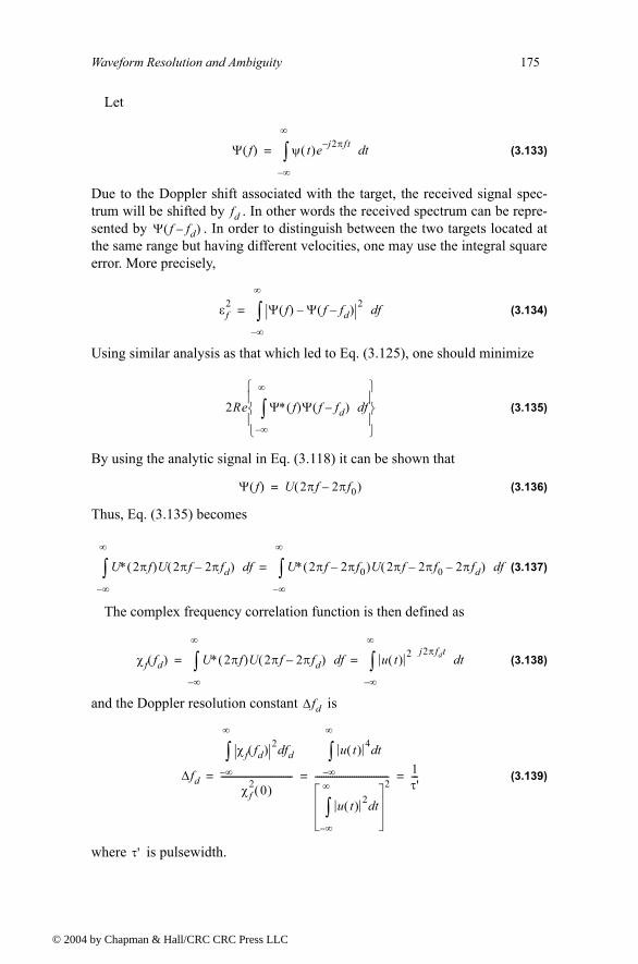
Waveform Resolution and Ambiguity 175
© 200
Let
(3.133)
Due to the Doppler shift associated with the target, the received signal spec-trum will be shifted by . In other words the received spectrum can be repre-sented by . In order to distinguish between the two targets located at the same range but having different velocities, one may use the integral square error. More precisely,
(3.134)
Using similar analysis as that which led to Eq. (3.125), one should minimize
(3.135)
By using the analytic signal in Eq. (3.118) it can be shown that
(3.136)
Thus, Eq. (3.135) becomes
(3.137)
The complex frequency correlation function is then defined as
(3.138)
and the Doppler resolution constant is
(3.139)
where is pulsewidth.
Ψ f( ) ψ t( )e j2πf t td∞
∞
∫=
fdΨ f fd( )
εf2 Ψ f( ) Ψ f fd( )
2 fd∞
∞
∫=
2Re Ψ∗ f( )Ψ f fd( ) fd∞
∞
∫
Ψ f( ) U 2πf 2πf0( )=
U∗ 2πf( )U 2πf 2πfd( ) fd∞
∞
∫ U∗ 2πf 2πf0( )U 2πf 2πf0 2πfd( ) fd∞
∞
∫=
χf fd( ) U∗ 2πf( )U 2πf 2πfd( ) fd∞
∞
∫ u t( ) 2 j2πfdttd
∞
∞
∫= =
∆fd
∆fd
χf fd( ) 2 fdd∞
∞
∫
χf2 0( )
---------------------------------
u t( ) 4 td∞
∞
∫
u t( ) 2 td∞
∞
∫2
---------------------------------- 1τ'---= = =
τ'
4 by Chapman & Hall/CRC CRC Press LLC
176 MATLAB Simulations for Radar Systems Design
© 200
Finally, one can define the corresponding velocity resolution as
(3.140)
Again observation of Eqs. (3.138) and (3.116) indicate that the output of the matched filter and the ambiguity function (when ) are similar to each other. Consequently, one concludes that the matched filter preserves the wave-form Doppler resolution properties as well.
3.10.3. Combined Range and Doppler Resolution
In this general case, one needs to use a two-dimensional function in the pair of variables ( ). For this purpose, assume that the complex envelope of the transmitted waveform is
(3.141)
Then the delayed and Doppler-shifted signal is
(3.142)
Computing the integral square error between Eqs. (3.142) and (3.141) yields
(3.143)
which can be written as
(3.144)
Again, in order to maximize this squared error for one must minimize the last term of Eq. (3.144).
Define the combined range and Doppler correlation function as
(3.145)
In order to achieve the most range and Doppler resolution, the modulus square of this function must be minimized for and . Note that the output of
∆vc∆fd2f0
----------- c2f0τ'-----------= =
τ 0=
τ fd,
ψ t( ) u t( )ej2πf0t
=
ψ' t τ( ) u t τ( )ej2π f0 fd( ) t τ( )
=
ε2 ψ t( ) ψ' t τ( )2 td
∞
∞
∫ 2 ψ t( ) 2 td∞
∞
∫ 2Re ψ∗ t( ) ψ' t τ( ) td∞
∞
∫
= =
ε2 2 u t( ) 2 td∞
∞
∫ 2Re ej2π f0 fd( )τ
u t( )u∗ t τ( )ej2πfdt
td∞
∞
∫
=
τ 0≠
χ τ fd,( ) u t( )u∗ t τ( )ej2πfdt
td∞
∞
∫=
τ 0≠ fd 0≠
4 by Chapman & Hall/CRC CRC Press LLC
MyRadar Design Case Study - Visit 3 177
© 200
the matched filter in Eq. (3.116) is identical to that given in Eq. (3.145). This means that the output of the matched filter exhibits maximum instantaneous SNR as well as the most achievable range and Doppler resolutions.
3.11. MyRadar Design Case Study - Visit 3
3.11.1. Problem Statement
Assuming a matched filter receiver, select a set of waveforms that can meet the design requirements as stated in the previous two chapters. Assume linear frequency modulation. Do not use more than a total of 5 waveforms. Modify the design so that the range resolution during the search mode, and
during tracking.
3.11.2. A Design
The major characteristics of radar waveforms include the waveforms energy, range resolution, and Doppler (or velocity) resolution. The pulse (waveform) energy is
(3.146)
where is the peak transmitted power and is the pulsewidth. Range resolu-tion is defined in Eq. (3.131), while the velocity resolution is in Eq. (3.140).
Close attention should be paid to the selection process of the pulsewidth. In this design we will assume that the pulse energy is the same as that computed in Chapter 2. The radar operating bandwidth during search and track are calcu-lated from Eq. (3.131) as
(3.147)
Since the design calls for a pulsed radar, then for each pulse transmitted (one PRI) the radar should not be allowed to receive any signal until that pulse has been completely transmitted. This limits the radar to a minimum operating range defined by
(3.148)
In this design choose . It follows that the minimum acceptable pulsewidth is .
∆R 30m=∆R 7.5m=
E Ptτ=
Pt τ
Bsearch
Btrack 3 108× 2 30×( )⁄ 5 MHz=
3 108× 2 7.5×( )⁄ 20 MHz=
=
Rmincτ2-----=
Rmin 15Km≥τmax 100µs≤
4 by Chapman & Hall/CRC CRC Press LLC
178 MATLAB Simulations for Radar Systems Design
© 200
For this design select 5 waveforms, one for search and four for track. Typi-cally search waveforms are longer than track waveforms; alternatively, track-ing waveforms require wider bandwidths than search waveforms. However, in the context of range, more energy is required at longer ranges (for both track and search waveforms), since one would expect the SNR to get larger as range becomes smaller. This was depicted in the example shown in Fig. 1.13 in Chapter 1.
Assume that during search and initial detection the single pulse peak power is to be kept under 10 KW (i.e., ). Then by using the single pulse energy calculated using Eq. (2.115) in Chapter 2, one can compute the mini-mum required pulsewidth as
(3.149)
Choose , with bandwidth and use LFM modulation. Fig. 3.18 shows plots of the real part, imaginary part, and the spectrum of this search waveform. This figure was produced using the GUI workspace LFM_gui.m. As far as the track waveforms, choose four waveforms of the same bandwidth ( ) and with the following pulsewidths.
Note that refers to the initial range at which track has been initiated. Fig. 3.19 is similar to Fig. 3.18 except it is for .
For the waveform set selected in this design option, the radar duty cycle var-ies from 1.25% to 2.0%. Remember that the PRF was calculated in Chapter 1 as ; thus the PRI is .
At this point of the design, one must verify that the selected waveforms pro-vide the radar with the desired SNR that meets or exceeds what was calculated in Chapter 2, and plotted in Fig. 2.21. In other words, one must now re-run these calculations and verify that the SNR has not been degraded. This task will be postponed until Chapter 5, where the radar equation with pulse com-pression is developed.
TABLE 3.1. MyRadar design case study track waveforms.
Pulsewidth Range window
Pt 20KW≤
τmin0.1147
20 103×--------------------≥ 5.735µs=
τsearch 20µs= B 5MHz=
Btrack 20MHz=
τt1 20µs= Rmax 0.75Rmax→
τt2 17.5µs= 0.75Rmax 0.5Rmax→
τt3 15µs= 0.5Rmax 0.25Rmax→
τt4 12.5µs= R 0.25Rmax≤
Rmaxτt3
fr 1KHz= T 1ms=
4 by Chapman & Hall/CRC CRC Press LLC
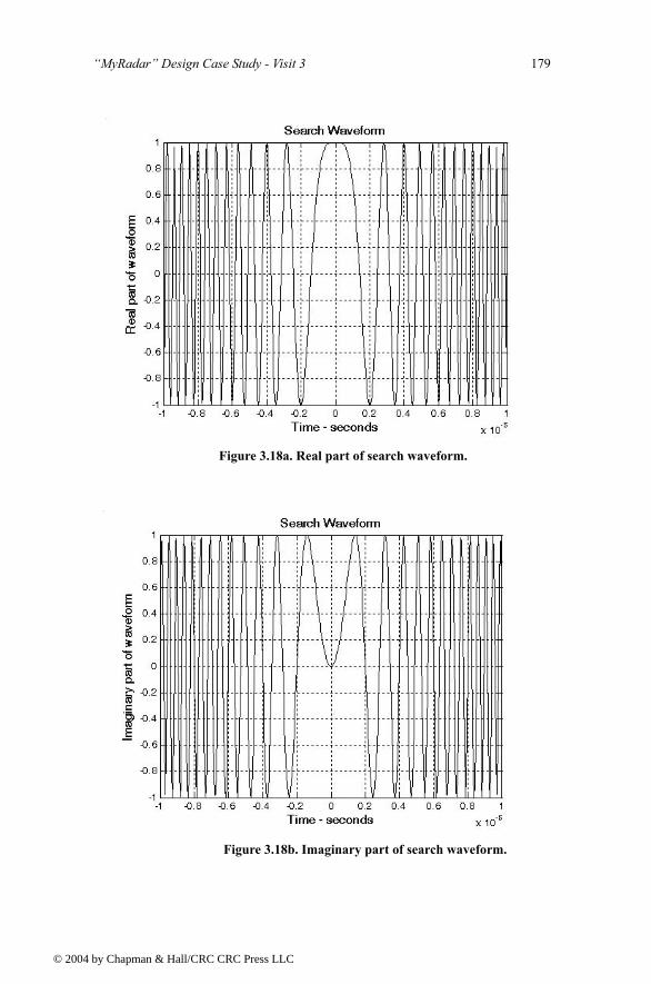
MyRadar Design Case Study - Visit 3 179
© 200
Figure 3.18a. Real part of search waveform.
Figure 3.18b. Imaginary part of search waveform.
4 by Chapman & Hall/CRC CRC Press LLC
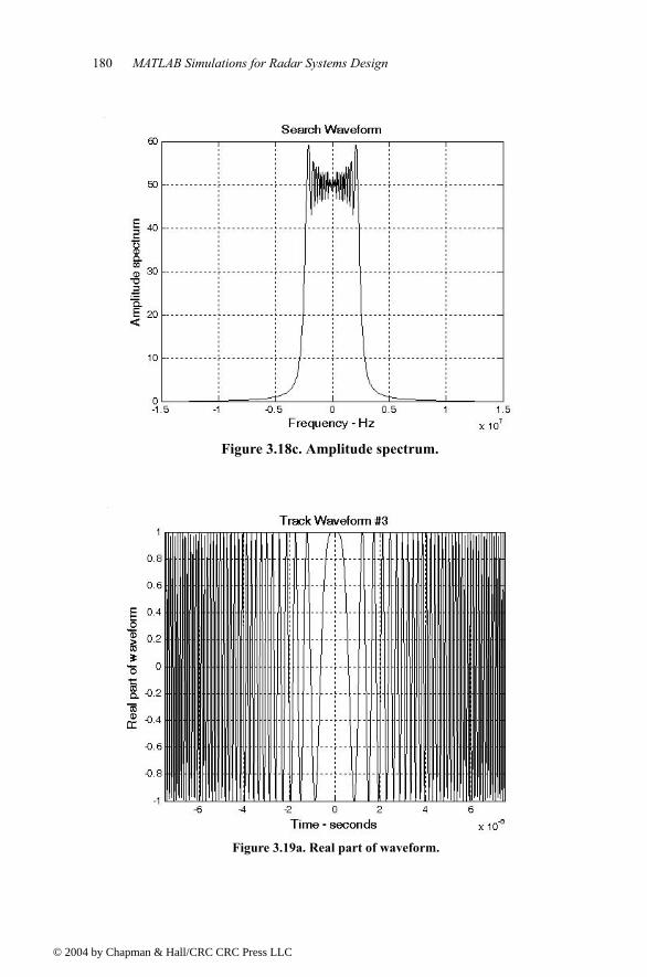
180 MATLAB Simulations for Radar Systems Design
© 200
Figure 3.18c. Amplitude spectrum.
Figure 3.19a. Real part of waveform.
4 by Chapman & Hall/CRC CRC Press LLC
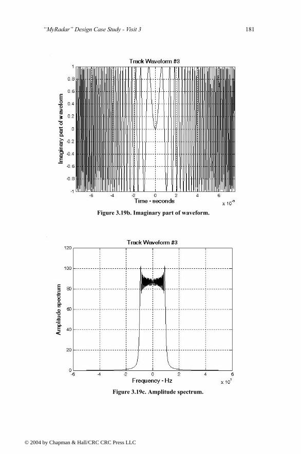
MyRadar Design Case Study - Visit 3 181
© 200
Figure 3.19b. Imaginary part of waveform.
Figure 3.19c. Amplitude spectrum.
4 by Chapman & Hall/CRC CRC Press LLC
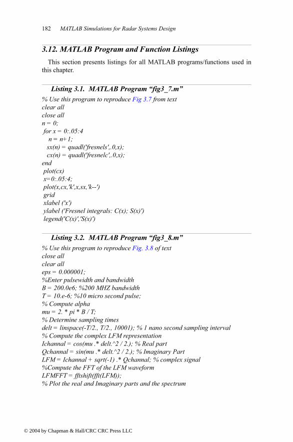
182 MATLAB Simulations for Radar Systems Design
© 200
3.12. MATLAB Program and Function ListingsThis section presents listings for all MATLAB programs/functions used in
this chapter.
Listing 3.1. MATLAB Program fig3_7.m% Use this program to reproduce Fig 3.7 from textclear allclose alln = 0; for x = 0:.05:4 n = n+1; sx(n) = quadl('fresnels',.0,x); cx(n) = quadl('fresnelc',.0,x);end plot(cx) x=0:.05:4; plot(x,cx,'k',x,sx,'k--') grid xlabel ('x') ylabel ('Fresnel integrals: C(x); S(x)') legend('C(x)','S(x)')
Listing 3.2. MATLAB Program fig3_8.m% Use this program to reproduce Fig. 3.8 of textclose allclear alleps = 0.000001;%Enter pulsewidth and bandwidthB = 200.0e6; %200 MHZ bandwidthT = 10.e-6; %10 micro second pulse;% Compute alphamu = 2. * pi * B / T;% Determine sampling timesdelt = linspace(-T/2., T/2., 10001); % 1 nano second sampling interval% Compute the complex LFM representationIchannal = cos(mu .* delt.^2 / 2.); % Real partQchannal = sin(mu .* delt.^2 / 2.); % Imaginary PartLFM = Ichannal + sqrt(-1) .* Qchannal; % complex signal%Compute the FFT of the LFM waveformLFMFFT = fftshift(fft(LFM));% Plot the real and Imaginary parts and the spectrum
4 by Chapman & Hall/CRC CRC Press LLC
MATLAB Program and Function Listings 183
© 200
freqlimit = 0.5 / 1.e-9;% the sampling interval 1 nano-secondfreq = linspace(-freqlimit/1.e6,freqlimit/1.e6,10001);figure(1)plot(delt*1e6,Ichannal,'k');axis([-1 1 -1 1])gridxlabel('Time - microsecs')ylabel('Real part')title('T = 10 Microsecond, B = 200 MHz')figure(2)plot(delt*1e6,Qchannal,'k');axis([-1 1 -1 1])gridxlabel('Time - microsecs')ylabel('Imaginary part')title('T = 10 Microsecond, B = 200 MHz')figure(3)plot(freq, abs(LFMFFT),'k');%axis tightgridxlabel('Frequency - MHz')ylabel('Amplitude spectrum')title('Spectrum for an LFM waveform and T = 10 Microsecond, ... B = 200 MHZ')
Listing 3.3. MATLAB Function hrr_profile.mfunction [hl] = hrr_profile (nscat, scat_range, scat_rcs, n, deltaf, prf, v,
rnote,winid)% Range or Time domain Profile% Range_Profile returns the Range or Time domain plot of a simulated % HRR SFWF returning from a predetermined number of targets with a prede-
termined% RCS for each target.c=3.0e8; % speed of light (m/s)num_pulses = n;SNR_dB = 40;nfft = 256;%carrier_freq = 9.5e9; %Hz (10GHz)freq_step = deltaf; %Hz (10MHz)V = v; % radial velocity (m/s) -- (+)=towards radar (-)=awayPRI = 1. / prf; % (s)if (nfft > 2*num_pulses) num_pulses = nfft/2;
4 by Chapman & Hall/CRC CRC Press LLC
184 MATLAB Simulations for Radar Systems Design
© 200
endInphase = zeros((2*num_pulses),1);Quadrature = zeros((2*num_pulses),1);Inphase_tgt = zeros(num_pulses,1);Quadrature_tgt = zeros(num_pulses,1);IQ_freq_domain = zeros((2*num_pulses),1);Weighted_I_freq_domain = zeros((num_pulses),1);Weighted_Q_freq_domain = zeros((num_pulses),1);Weighted_IQ_time_domain = zeros((2*num_pulses),1);Weighted_IQ_freq_domain = zeros((2*num_pulses),1);abs_Weighted_IQ_time_domain = zeros((2*num_pulses),1);dB_abs_Weighted_IQ_time_domain = zeros((2*num_pulses),1);taur = 2. * rnote / c;for jscat = 1:nscat ii = 0; for i = 1:num_pulses ii = ii+1; rec_freq = ((i-1)*freq_step); Inphase_tgt(ii) = Inphase_tgt(ii) + sqrt(scat_rcs(jscat)) * cos(-
2*pi*rec_freq*... (2.*scat_range(jscat)/c - 2*(V/c)*((i-1)*PRI + taur/2 +
2*scat_range(jscat)/c))); Quadrature_tgt(ii) = Quadrature_tgt(ii) + sqrt(scat_rcs(jscat))*sin(-
2*pi*rec_freq*... (2*scat_range(jscat)/c - 2*(V/c)*((i-1)*PRI + taur/2 +
2*scat_range(jscat)/c))); endendif(winid >= 0) window(1:num_pulses) = hamming(num_pulses);else window(1:num_pulses) = 1;endInphase = Inphase_tgt;Quadrature = Quadrature_tgt;Weighted_I_freq_domain(1:num_pulses) = Inphase(1:num_pulses).* window';Weighted_Q_freq_domain(1:num_pulses) = Quadrature(1:num_pulses).* win-
dow';Weighted_IQ_freq_domain(1:num_pulses)= Weighted_I_freq_domain + ... Weighted_Q_freq_domain*j;Weighted_IQ_freq_domain(num_pulses:2*num_pulses)=0.+0.i;Weighted_IQ_time_domain = (ifft(Weighted_IQ_freq_domain));abs_Weighted_IQ_time_domain = (abs(Weighted_IQ_time_domain));
4 by Chapman & Hall/CRC CRC Press LLC
MATLAB Program and Function Listings 185
© 200
dB_abs_Weighted_IQ_time_domain = 20.0*log10(abs_Weighted_IQ_time_domain)+SNR_dB;
% calculate the unambiguous range window sizeRu = c /2/deltaf;hl = dB_abs_Weighted_IQ_time_domain;numb = 2*num_pulses;delx_meter = Ru / numb;xmeter = 0:delx_meter:Ru-delx_meter;plot(xmeter, dB_abs_Weighted_IQ_time_domain,'k')xlabel ('relative distance - meters')ylabel ('Range profile - dB')grid
Listing 3.4. MATLAB Program fig3_17.m% use this program to reproduce Fig. 3.17 of textclear allclose allnscat = 1;scat_range = 912;scat_rcs = 10;n =64;deltaf = 10e6;prf = 10e3;v = 15;rnote = 900,winid = 1;count = 0;for time = 0:.05:3 count = count +1; hl = hrr_profile (nscat, scat_range, scat_rcs, n, deltaf, prf, v, rnote,winid); array(count,:) = transpose(hl); hl(1:end) = 0; scat_range = scat_range - 2 * n * v / prf;endfigure (1) numb = 2*256;% this number matches that used in hrr_profile. delx_meter = 15 / numb; xmeter = 0:delx_meter:15-delx_meter; imagesc(xmeter, 0:0.05:4,array) colormap(gray)ylabel ('Time in seconds')xlabel('Relative distance in meters')
4 by Chapman & Hall/CRC CRC Press LLC

186 MATLAB Simulations for Radar Systems Design
© 200
4 by Chapman & Hall/CRC CRC Press LLC
© 200
Chapter 4 The Radar Ambiguity Function
4.1. IntroductionThe radar ambiguity function represents the output of the matched filter, and
it describes the interference caused by the range and/or Doppler shift of a tar-get when compared to a reference target of equal RCS. The ambiguity function evaluated at is equal to the matched filter output that is matched perfectly to the signal reflected from the target of interest. In other words, returns from the nominal target are located at the origin of the ambigu-ity function. Thus, the ambiguity function at nonzero and represents returns from some range and Doppler different from those for the nominal tar-get.
The radar ambiguity function is normally used by radar designers as a means of studying different waveforms. It can provide insight about how different radar waveforms may be suitable for the various radar applications. It is also used to determine the range and Doppler resolutions for a specific radar wave-form. The three-dimensional (3-D) plot of the ambiguity function versus fre-quency and time delay is called the radar ambiguity diagram. The radar ambiguity function for the signal is defined as the modulus squared of its 2-D correlation function, i.e., . More precisely,
(4.1)
In this notation, the target of interest is located at , and the ambiguity diagram is centered at the same point. Note that some authors define the ambiguity function as . In this book, is called the uncer-tainty function.
τ fd,( ) 0 0,( )=
τ fd
s t( )χ τ fd;( ) 2
χ τ fd;( ) 2 s t( )s∗ t τ( )ej2πfdt
td
∞
∞
∫2
=
τ fd,( ) 0 0,( )=
χ τ fd;( ) χ τ fd;( )
4 by Chapman & Hall/CRC CRC Press LLC
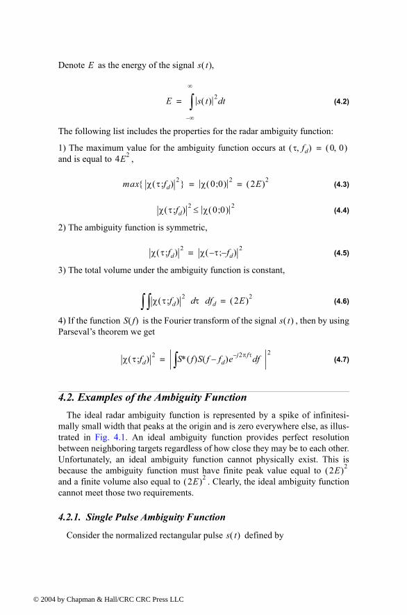
© 200
Denote as the energy of the signal ,
(4.2)
The following list includes the properties for the radar ambiguity function:
1) The maximum value for the ambiguity function occurs at and is equal to ,
(4.3)
(4.4)
2) The ambiguity function is symmetric,
(4.5)
3) The total volume under the ambiguity function is constant,
(4.6)
4) If the function is the Fourier transform of the signal , then by using Parsevals theorem we get
(4.7)
4.2. Examples of the Ambiguity FunctionThe ideal radar ambiguity function is represented by a spike of infinitesi-
mally small width that peaks at the origin and is zero everywhere else, as illus-trated in Fig. 4.1. An ideal ambiguity function provides perfect resolution between neighboring targets regardless of how close they may be to each other. Unfortunately, an ideal ambiguity function cannot physically exist. This is because the ambiguity function must have finite peak value equal to and a finite volume also equal to . Clearly, the ideal ambiguity function cannot meet those two requirements.
4.2.1. Single Pulse Ambiguity Function
Consider the normalized rectangular pulse defined by
E s t( )
E s t( ) 2 td
∞
∞
∫=
τ fd,( ) 0 0,( )=4E2
max χ τ fd;( ) 2 χ 0 0;( ) 2 2E( )2= =
χ τ fd;( ) 2 χ 0 0;( ) 2≤
χ τ fd;( ) 2 χ τ f d;( ) 2=
χ τ fd;( ) 2 τd fdd∫∫ 2E( )2=
S f( ) s t( )
χ τ fd;( ) 2 S∗ f( )S f fd( )e j2πfτ fd∫2
=
2E( )2
2E( )2
s t( )
4 by Chapman & Hall/CRC CRC Press LLC
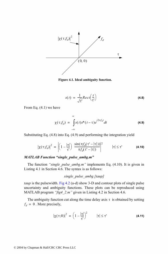
© 200
(4.8)
From Eq. (4.1) we have
(4.9)
Substituting Eq. (4.8) into Eq. (4.9) and performing the integration yield
(4.10)
MATLAB Function single_pulse_ambg.m
The function single_pulse_ambg.m implements Eq. (4.10). It is given in Listing 4.1 in Section 4.6. The syntax is as follows:
single_pulse_ambg [taup]
taup is the pulsewidth. Fig 4.2 (a-d) show 3-D and contour plots of single pulse uncertainty and ambiguity functions. These plots can be reproduced using MATLAB program fig4_2.m given in Listing 4.2 in Section 4.6.
The ambiguity function cut along the time delay axis is obtained by setting . More precisely,
(4.11)
τ
fdχ τ fd;( ) 2
0 0,( )
Figure 4.1. Ideal ambiguity function.
s t( ) 1τ'
-------Rect tτ'--- =
χ τ fd;( ) s t( )s∗ t τ( )ej2πfdt
td
∞
∞
∫=
χ τ fd;( ) 2 1 ττ'-----
πfd τ' τ( )( )sinπfd τ' τ( )
----------------------------------------2
= τ τ'≤
τfd 0=
χ τ 0;( ) 2 1 ττ'-----
2= τ τ'≤
4 by Chapman & Hall/CRC CRC Press LLC
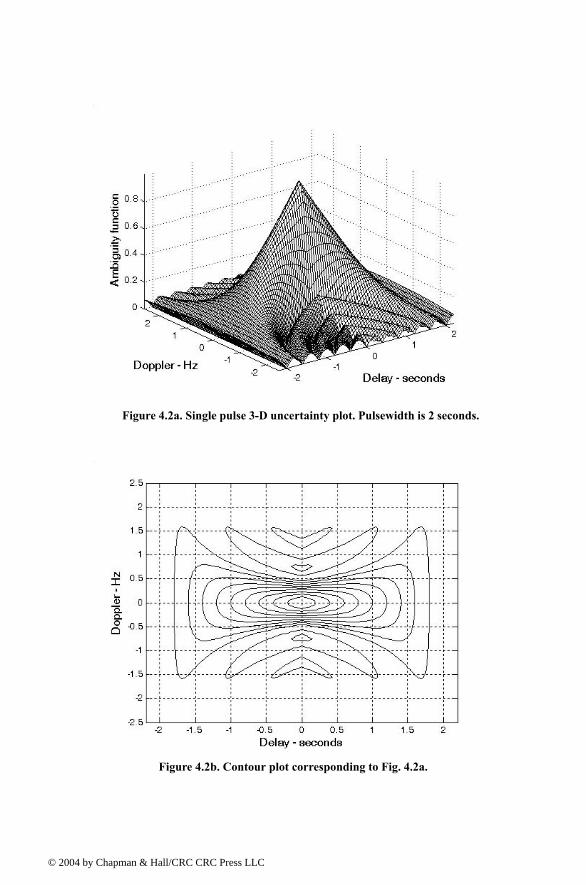
© 200
Figure 4.2a. Single pulse 3-D uncertainty plot. Pulsewidth is 2 seconds.
Figure 4.2b. Contour plot corresponding to Fig. 4.2a.
4 by Chapman & Hall/CRC CRC Press LLC
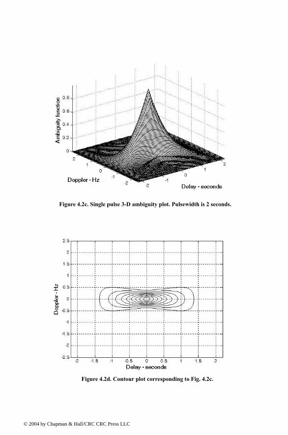
© 200
Figure 4.2c. Single pulse 3-D ambiguity plot. Pulsewidth is 2 seconds.
Figure 4.2d. Contour plot corresponding to Fig. 4.2c.
4 by Chapman & Hall/CRC CRC Press LLC
© 200
Note that the time autocorrelation function of the signal is equal to . Similarly, the cut along the Doppler axis is
(4.12)
Figs. 4.3 and 4.4, respectively, show the plots of the uncertainty function cuts defined by Eqs. (4.11) and (4.12). Since the zero Doppler cut along the time delay axis extends between and , then, close targets would be unambiguous if they are at least seconds apart.
s t( )χ τ 0;( )
χ 0 fd;( ) 2 πτ'fdsinπτ'fd
-------------------2
=
τ' τ'τ'
τ'τ ' τ
amplitude
Figure 4.3. Zero Doppler uncertainty function cut along the time delay axis.
Figure 4.4. Uncertainty function of a single frequency pulse (zero delay). This plot can be reproduced using MATLAB program fig4_4.m given in Listing 4.3 in Section 4.6.
4 by Chapman & Hall/CRC CRC Press LLC
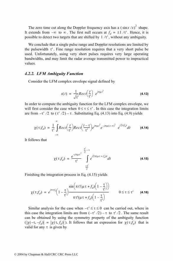
© 200
The zero time cut along the Doppler frequency axis has a shape. It extends from to . The first null occurs at . Hence, it is possible to detect two targets that are shifted by , without any ambiguity.
We conclude that a single pulse range and Doppler resolutions are limited by the pulsewidth . Fine range resolution requires that a very short pulse be used. Unfortunately, using very short pulses requires very large operating bandwidths, and may limit the radar average transmitted power to impractical values.
4.2.2. LFM Ambiguity Function
Consider the LFM complex envelope signal defined by
(4.13)
In order to compute the ambiguity function for the LFM complex envelope, we will first consider the case when . In this case the integration limits are from to . Substituting Eq. (4.13) into Eq. (4.9) yields
(4.14)
It follows that
(4.15)
Finishing the integration process in Eq. (4.15) yields
(4.16)
Similar analysis for the case when can be carried out, where in this case the integration limits are from to . The same result can be obtained by using the symmetry property of the ambiguity function ( ). It follows that an expression for that is valid for any is given by
xsin x⁄( )2
∞ ∞ fd 1 τ'⁄±=1 τ'⁄
τ'
s t( ) 1τ'
-------Rect tτ'--- ejπµt2
=
0 τ τ′≤ ≤τ′ 2⁄ τ′ 2⁄( ) τ
χ τ fd;( ) 1τ′---- Rect t
τ′---- Rect t τ
τ′---------- ejπµt2
e jπµ t τ( )2 ej2πfdt
∞
∞
∫ dt=
χ τ fd;( ) e j πµτ2
τ'--------------- e
j2π µτ f+ d( )t
τ'2
------
τ'2--- τ
∫ dt=
χ τ fd;( ) ejπτfd 1 τ
τ'---
πτ' µτ fd+( ) 1 τ
τ'---
sin
πτ' µτ fd+( ) 1 ττ'---
-------------------------------------------------------------= 0 τ τ′≤ ≤
τ′ τ 0≤ ≤τ′ 2⁄( ) τ τ' 2⁄
χ τ fd,( ) χ τ fd,( )= χ τ fd;( )τ
4 by Chapman & Hall/CRC CRC Press LLC
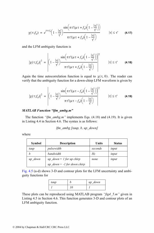
© 200
(4.17)
and the LFM ambiguity function is
(4.18)
Again the time autocorrelation function is equal to . The reader can verify that the ambiguity function for a down-chirp LFM waveform is given by
(4.19)
MATLAB Function lfm_ambg.m
The function lfm_ambg.m implements Eqs. (4.18) and (4.19). It is given in Listing 4.4 in Section 4.6. The syntax is as follows:
lfm_ambg [taup, b, up_down]
where
Fig. 4.5 (a-d) shows 3-D and contour plots for the LFM uncertainty and ambi-guity functions for
These plots can be reproduced using MATLAB program fig4_5.m given in Listing 4.5 in Section 4.6. This function generates 3-D and contour plots of an LFM ambiguity function.
Symbol Description Units Status
taup pulsewidth seconds input
b bandwidth Hz input
up_down up_down = 1 for up chirp
up_down = -1 for down chirp
none input
taup b up_down
1 10 1
χ τ fd;( ) ejπτfd 1 τ
τ'-----
πτ' µτ fd+( ) 1 τ
τ'-----
sin
πτ' µτ fd+( ) 1 ττ'-----
---------------------------------------------------------------= τ τ'≤
χ τ fd;( ) 2 1 ττ'-----
πτ' µτ fd+( ) 1 τ
τ'-----
sin
πτ' µτ fd+( ) 1 ττ'-----
---------------------------------------------------------------
2
= τ τ'≤
χ τ 0,( )
χ τ fd;( ) 2 1 ττ'-----
πτ' µτ fd( ) 1 τ
τ'-----
sin
πτ' µτ fd( ) 1 ττ'-----
---------------------------------------------------------------
2
= τ τ'≤
4 by Chapman & Hall/CRC CRC Press LLC
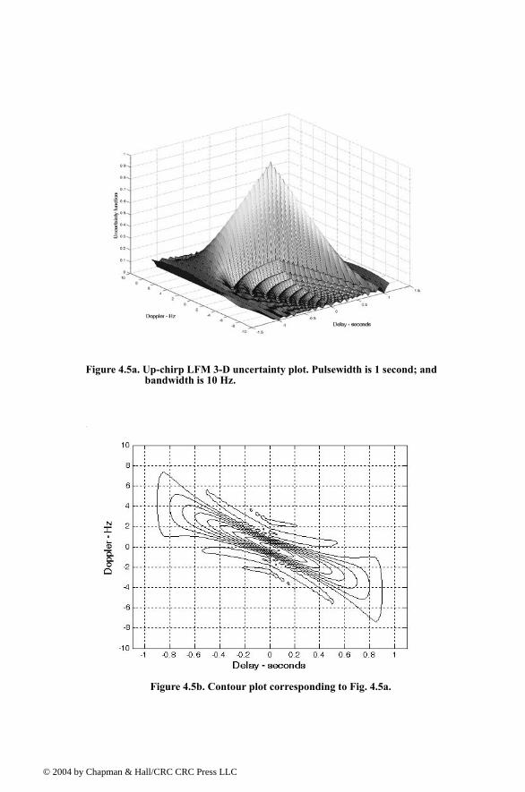
© 200
Figure 4.5a. Up-chirp LFM 3-D uncertainty plot. Pulsewidth is 1 second; and bandwidth is 10 Hz.
Figure 4.5b. Contour plot corresponding to Fig. 4.5a.
4 by Chapman & Hall/CRC CRC Press LLC
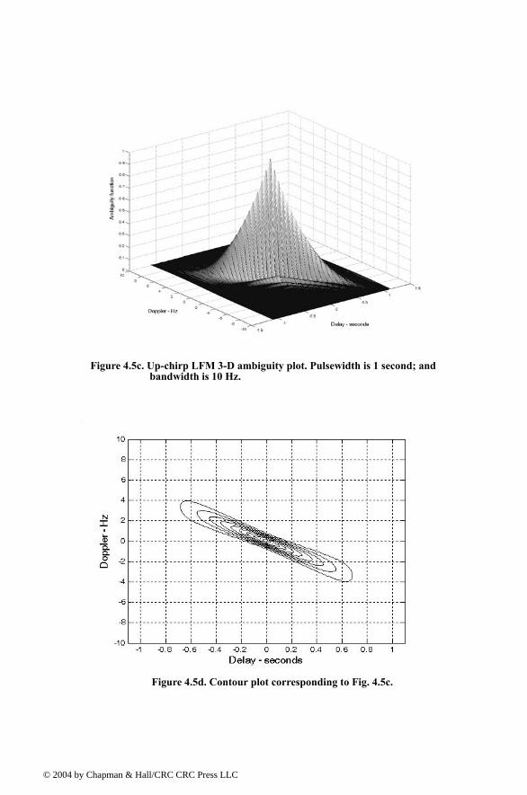
© 200
Figure 4.5c. Up-chirp LFM 3-D ambiguity plot. Pulsewidth is 1 second; and bandwidth is 10 Hz.
Figure 4.5d. Contour plot corresponding to Fig. 4.5c.
4 by Chapman & Hall/CRC CRC Press LLC
© 200
The up-chirp ambiguity function cut along the time delay axis is
(4.20)
Fig. 4.6 shows a plot for a cut in the uncertainty function corresponding to Eq. (4.20). Note that the LFM ambiguity function cut along the Doppler fre-quency axis is similar to that of the single pulse. This should not be surprising since the pulse shape has not changed (we only added frequency modulation). However, the cut along the time delay axis changes significantly. It is now much narrower compared to the unmodulated pulse cut. In this case, the first null occurs at
(4.21)
which indicates that the effective pulsewidth (compressed pulsewidth) of the matched filter output is completely determined by the radar bandwidth. It fol-lows that the LFM ambiguity function cut along the time delay axis is narrower than that of the unmodulated pulse by a factor
τ
χ τ 0;( ) 2 1 ττ'-----
πµττ' 1 τ
τ'-----
sin
πµττ' 1 ττ'-----
------------------------------------------------
2
= τ τ'≤
τn1 1 B⁄≈
Figure 4.6. Zero Doppler uncertainty of an LFM pulse ( , ). This plot can be reproduced using MATLAB
program fig4_6.m given in Listing 4.6 in Section 4.6.
τ′ 1=b 20=
4 by Chapman & Hall/CRC CRC Press LLC
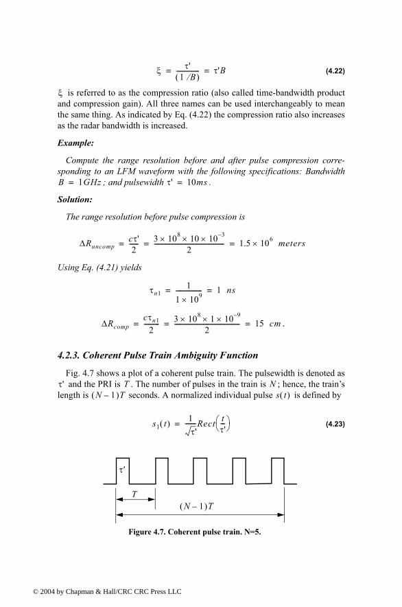
© 200
(4.22)
is referred to as the compression ratio (also called time-bandwidth product and compression gain). All three names can be used interchangeably to mean the same thing. As indicated by Eq. (4.22) the compression ratio also increases as the radar bandwidth is increased.
Example:
Compute the range resolution before and after pulse compression corre-sponding to an LFM waveform with the following specifications: Bandwidth
; and pulsewidth .
Solution:
The range resolution before pulse compression is
Using Eq. (4.21) yields
.
4.2.3. Coherent Pulse Train Ambiguity Function
Fig. 4.7 shows a plot of a coherent pulse train. The pulsewidth is denoted as and the PRI is . The number of pulses in the train is ; hence, the trains
length is seconds. A normalized individual pulse is defined by
(4.23)
ξ τ'1 B⁄( )
--------------- τ'B= =
ξ
B 1GHz= τ' 10ms=
∆Runcompcτ'2
------ 3 108× 10 10 3××2
---------------------------------------------- 1.5 106× meters= = =
τn11
1 109×----------------- 1 ns= =
∆Rcompcτn1
2---------- 3 108× 1 10 9××
2------------------------------------------- 15 cm= = =
τ' T NN 1( )T s t( )
s1 t( ) 1τ'
-------Rect tτ'--- =
N 1( )TT
τ′
Figure 4.7. Coherent pulse train. N=5.
4 by Chapman & Hall/CRC CRC Press LLC
© 200
When coherency is maintained between the consecutive pulses, then an expres-sion for the normalized train is
(4.24)
The output of the matched filter is
(4.25)
Substituting Eq. (4.24) into Eq. (4.25) and interchanging the summations and integration yield
(4.26)
Making the change of variable yields
(4.27)
The integral inside Eq. (4.27) represents the output of the matched filter for a single pulse, and is denoted by . It follows that
(4.28)
When the relation is used, then the following relation is true:1
(4.29)
Using Eq. (4.29) into Eq. (4.28) gives
1. Rihaczek, A. W., Principles of High Resolution Radar, Artech House, 1994.
s t( ) 1N
-------- s1 t iT( )
i 0=
N 1
∑=
χ τ fd;( ) s t( )s∗ t τ+( )ej2πfdt
td
∞
∞
∫=
χ τ fd;( ) 1N---- s1 t iT( ) s1∗ t jT τ( )e
j2πfdttd
∞
∞
∫j 0=
N 1
∑i 0=
N 1
∑=
t1 t iT=
χ τ fd;( ) 1N---- e
j2πfdiTs1 t1( ) s1∗ t1 τ i j( )T[ ]( )e
j2πfdt1 t1d
∞
∞
∫j 0=
N 1
∑i 0=
N 1
∑=
χ1
χ τ fd;( ) 1N---- e
j2πfdiTχ1 τ i j( )T fd;[ ]
j 0=
N 1
∑i 0=
N 1
∑=
q i j=
m 0=
N
∑i 0=
N
∑i 0=
N 1 q
∑for j i q=q N 1( )=
0
∑j 0=
N 1 q
∑for i j q+=q 1=
N 1
∑+=
4 by Chapman & Hall/CRC CRC Press LLC
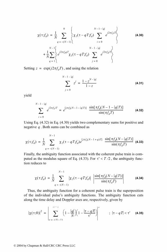
© 200
(4.30)
Setting , and using the relation
(4.31)
yield
(4.32)
Using Eq. (4.32) in Eq. (4.30) yields two complementary sums for positive and negative . Both sums can be combined as
(4.33)
Finally, the ambiguity function associated with the coherent pulse train is com-puted as the modulus square of Eq. (4.33). For , the ambiguity func-tion reduces to
(4.34)
Thus, the ambiguity function for a coherent pulse train is the superposition of the individual pulses ambiguity functions. The ambiguity function cuts along the time delay and Doppler axes are, respectively, given by
(4.35)
χ τ fd;( ) 1N---- χ1 τ qT fd;( ) e
j2πfdiT
i 0=
N 1 q
∑
1N---- e
j2πfdqTχ1 τ qT fd;( ) e
j2πfdjT
j 0=
N 1 q
∑
q 1=
N 1
∑+
q N 1( )=
0
∑=
z j2πfdT( )exp=
zj
j 0=
N 1 q
∑ 1 zN q1 z
----------------------=
ej2πfdiT
i 0=
N 1 q
∑ ejπfd N 1 q T( )[ ] πfd N 1 q T( )[ ]sin
πfdT( )sin------------------------------------------------------=
q
χ τ fd;( ) 1N---- χ1 τ qT fd;( )e
jπfd N 1 q+( )T[ ] πfd N q T( )[ ]sinπfdT( )sin
---------------------------------------------
q N 1( )=
N 1
∑=
τ′ T 2⁄<
χ τ fd;( ) 1N---- χ1 τ qT fd;( ) πfd N q T( )[ ]sin
πfdT( )sin---------------------------------------------
q N 1( )=
N 1
∑=
χ τ 0;( ) 2 1 qN-----
1 τ qTτ′
------------------
q N 1( )=
N 1
∑2
= τ qT τ′<;
4 by Chapman & Hall/CRC CRC Press LLC

© 200
(4.36)
MATLAB Function train_ambg.m
The function train_ambg.m implements Eq. (4.34). It is given in Listing 4.7 in Section 4.6. The syntax is as follows:
train_ambg [taup, n, pri]
Fig. 4.8 (a-d) shows typical outputs of this function, for
Symbol Description Units Status
taup pulsewidth seconds input
n number of pulses in train none input
pri pulse repetition interval seconds input
taup n pri
0.2 5 1
χ 0 fd;( ) 2 1N----
πfdτ′( )sinπfdτ′
-------------------------πfdNT( )sinπfdT( )sin
----------------------------2
=
Figure 4.8a. Three-dimensional ambiguity plot for a five pulse equal amplitude coherent train. Pulsewidth is 0.2 seconds; and PRI is 1 second, N=5. This plot can be reproduced using MATLAB program fig4_8.m given in Listing 4.8 in Section 4.6.
4 by Chapman & Hall/CRC CRC Press LLC
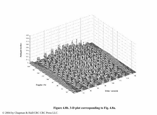
.
© 2004 by Chapman & Hall/CRC CRC Press LLC
Figure 4.8b. 3-D plot corresponding to Fig. 4.8a© 2004 by Chapman & Hall/CRC CRC Press LLC
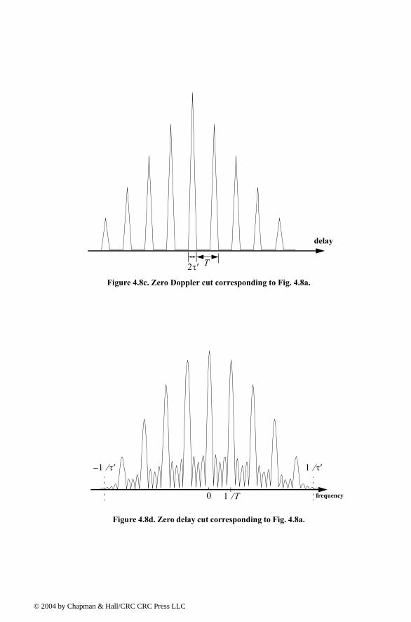
© 200
Figure 4.8c. Zero Doppler cut corresponding to Fig. 4.8a.
2τ′ T
delay
Figure 4.8d. Zero delay cut corresponding to Fig. 4.8a.
0 1 T⁄ frequency
1 τ′⁄ 1 τ′⁄
4 by Chapman & Hall/CRC CRC Press LLC
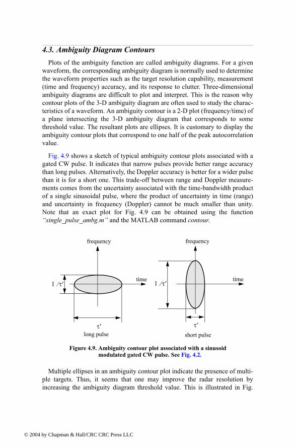
© 200
4.3. Ambiguity Diagram ContoursPlots of the ambiguity function are called ambiguity diagrams. For a given
waveform, the corresponding ambiguity diagram is normally used to determine the waveform properties such as the target resolution capability, measurement (time and frequency) accuracy, and its response to clutter. Three-dimensional ambiguity diagrams are difficult to plot and interpret. This is the reason why contour plots of the 3-D ambiguity diagram are often used to study the charac-teristics of a waveform. An ambiguity contour is a 2-D plot (frequency/time) of a plane intersecting the 3-D ambiguity diagram that corresponds to some threshold value. The resultant plots are ellipses. It is customary to display the ambiguity contour plots that correspond to one half of the peak autocorrelation value.
Fig. 4.9 shows a sketch of typical ambiguity contour plots associated with a gated CW pulse. It indicates that narrow pulses provide better range accuracy than long pulses. Alternatively, the Doppler accuracy is better for a wider pulse than it is for a short one. This trade-off between range and Doppler measure-ments comes from the uncertainty associated with the time-bandwidth product of a single sinusoidal pulse, where the product of uncertainty in time (range) and uncertainty in frequency (Doppler) cannot be much smaller than unity. Note that an exact plot for Fig. 4.9 can be obtained using the function single_pulse_ambg.m and the MATLAB command contour.
Multiple ellipses in an ambiguity contour plot indicate the presence of multi-ple targets. Thus, it seems that one may improve the radar resolution by increasing the ambiguity diagram threshold value. This is illustrated in Fig.
time
frequency frequency
time
τ′ τ′
1 τ′⁄1 τ′⁄
long pulse short pulse
Figure 4.9. Ambiguity contour plot associated with a sinusoid modulated gated CW pulse. See Fig. 4.2.
4 by Chapman & Hall/CRC CRC Press LLC
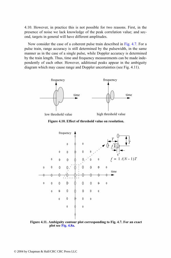
© 200
4.10. However, in practice this is not possible for two reasons. First, in the presence of noise we lack knowledge of the peak correlation value; and sec-ond, targets in general will have different amplitudes.
Now consider the case of a coherent pulse train described in Fig. 4.7. For a pulse train, range accuracy is still determined by the pulsewidth, in the same manner as in the case of a single pulse, while Doppler accuracy is determined by the train length. Thus, time and frequency measurements can be made inde-pendently of each other. However, additional peaks appear in the ambiguity diagram which may cause range and Doppler uncertainties (see Fig. 4.11).
time
frequency
time
frequency
low threshold value high threshold value
Figure 4.10. Effect of threshold value on resolution.
frequency
time
1T---T
τ′
f
f
1 N 1( )T⁄=
Figure 4.11. Ambiguity contour plot corresponding to Fig. 4.7. For an exact plot see Fig. 4.8a.
4 by Chapman & Hall/CRC CRC Press LLC
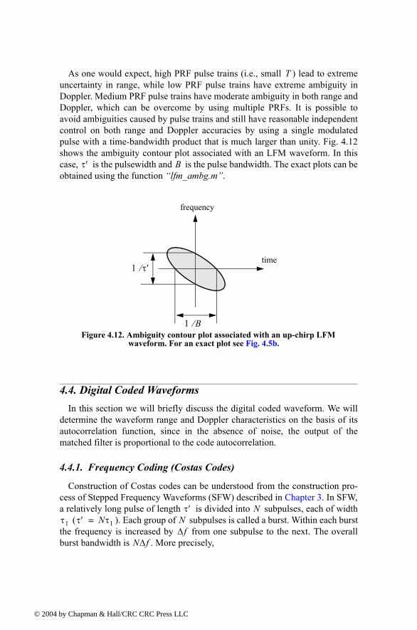
© 200
As one would expect, high PRF pulse trains (i.e., small ) lead to extreme uncertainty in range, while low PRF pulse trains have extreme ambiguity in Doppler. Medium PRF pulse trains have moderate ambiguity in both range and Doppler, which can be overcome by using multiple PRFs. It is possible to avoid ambiguities caused by pulse trains and still have reasonable independent control on both range and Doppler accuracies by using a single modulated pulse with a time-bandwidth product that is much larger than unity. Fig. 4.12 shows the ambiguity contour plot associated with an LFM waveform. In this case, is the pulsewidth and is the pulse bandwidth. The exact plots can be obtained using the function lfm_ambg.m.
4.4. Digital Coded WaveformsIn this section we will briefly discuss the digital coded waveform. We will
determine the waveform range and Doppler characteristics on the basis of its autocorrelation function, since in the absence of noise, the output of the matched filter is proportional to the code autocorrelation.
4.4.1. Frequency Coding (Costas Codes)
Construction of Costas codes can be understood from the construction pro-cess of Stepped Frequency Waveforms (SFW) described in Chapter 3. In SFW, a relatively long pulse of length is divided into subpulses, each of width
( ). Each group of subpulses is called a burst. Within each burst the frequency is increased by from one subpulse to the next. The overall burst bandwidth is . More precisely,
T
τ′ B
time
frequency
1 τ′⁄
1 B⁄ Figure 4.12. Ambiguity contour plot associated with an up-chirp LFM
waveform. For an exact plot see Fig. 4.5b.
τ′ Nτ1 τ′ Nτ1= N
∆fN∆f
4 by Chapman & Hall/CRC CRC Press LLC
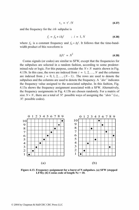
© 200
(4.37)
and the frequency for the subpulse is
(4.38)
where is a constant frequency and . It follows that the time-band-width product of this waveform is
(4.39)
Costas signals (or codes) are similar to SFW, except that the frequencies for the subpulses are selected in a random fashion, according to some predeter-mined rule or logic. For this purpose, consider the matrix shown in Fig. 4.13b. In this case, the rows are indexed from and the columns are indexed from . The rows are used to denote the subpulses and the columns are used to denote the frequency. A dot indicates the frequency value assigned to the associated subpulse. In this fashion, Fig. 4.13a shows the frequency assignment associated with a SFW. Alternatively, the frequency assignments in Fig. 4.13b are chosen randomly. For a matrix of size , there are a total of possible ways of assigning the dots (i.e.,
possible codes).
τ1 τ′ N⁄=
ith
fi f0 i∆f+= i; 1 N,=
f0 f0 ∆f»
∆fτ′ N2=
N N×i 1 2 … N, , ,=
j 0 1 2 … N 1( ), , , ,=
N N× N!N!
Figure 4.13. Frequency assignment for a burst of N subpulses. (a) SFW (stepped LFM); (b) Costas code of length Nc = 10.
(b)(a)
12345678910
12345678910
98765432109876543210
4 by Chapman & Hall/CRC CRC Press LLC
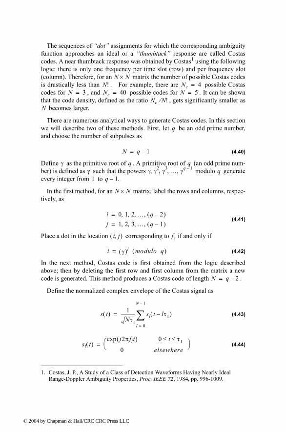
© 200
The sequences of dot assignments for which the corresponding ambiguity function approaches an ideal or a thumbtack response are called Costas codes. A near thumbtack response was obtained by Costas1 using the following logic: there is only one frequency per time slot (row) and per frequency slot (column). Therefore, for an matrix the number of possible Costas codes is drastically less than . For example, there are possible Costas codes for , and possible codes for . It can be shown that the code density, defined as the ratio , gets significantly smaller as
becomes larger.
There are numerous analytical ways to generate Costas codes. In this section we will describe two of these methods. First, let be an odd prime number, and choose the number of subpulses as
(4.40)
Define as the primitive root of . A primitive root of (an odd prime num-ber) is defined as such that the powers modulo generate every integer from to .
In the first method, for an matrix, label the rows and columns, respec-tively, as
(4.41)
Place a dot in the location corresponding to if and only if
(4.42)
In the next method, Costas code is first obtained from the logic described above; then by deleting the first row and first column from the matrix a new code is generated. This method produces a Costas code of length .
Define the normalized complex envelope of the Costas signal as
(4.43)
(4.44)
1. Costas, J. P., A Study of a Class of Detection Waveforms Having Nearly Ideal Range-Doppler Ambiguity Properties, Proc. IEEE 72, 1984, pp. 996-1009.
N N×N! Nc 4=
N 3= Nc 40= N 5=Nc N!⁄
N
q
N q 1=
γ q qγ γ γ2 γ3 … γq 1, , , , q
1 q 1
N N×
i 0 1 2 … q 2( ), , , ,=
j 1 2 3 … q 1( ), , , ,=
i j,( ) fi
i γ( )j modulo q( )=
N q 2=
s t( ) 1Nτ1
------------- sl t lτ1( )
l 0=
N 1
∑=
sl t( )j2πflt( )exp
0=
0 t τ1≤ ≤
elsewhere
4 by Chapman & Hall/CRC CRC Press LLC
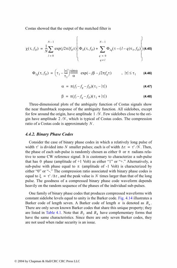
© 200
Costas showed that the output of the matched filter is
(4.45)
(4.46)
(4.47)
(4.48)
Three-dimensional plots of the ambiguity function of Costas signals show the near thumbtack response of the ambiguity function. All sidelobes, except for few around the origin, have amplitude . Few sidelobes close to the ori-gin have amplitude , which is typical of Costas codes. The compression ratio of a Costas code is approximately .
4.4.2. Binary Phase Codes
Consider the case of binary phase codes in which a relatively long pulse of width is divided into smaller pulses; each is of width . Then, the phase of each sub-pulse is randomly chosen as either or radians rela-tive to some CW reference signal. It is customary to characterize a sub-pulse that has phase (amplitude of +1 Volt) as either 1 or +. Alternatively, a sub-pulse with phase equal to (amplitude of -1 Volt) is characterized by either 0 or -. The compression ratio associated with binary phase codes is equal to , and the peak value is times larger than that of the long pulse. The goodness of a compressed binary phase code waveform depends heavily on the random sequence of the phases of the individual sub-pulses.
One family of binary phase codes that produces compressed waveforms with constant sidelobe levels equal to unity is the Barker code. Fig. 4.14 illustrates a Barker code of length seven. A Barker code of length is denoted as . There are only seven known Barker codes that share this unique property; they are listed in Table 4.1. Note that and have complementary forms that have the same characteristics. Since there are only seven Barker codes, they are not used when radar security is an issue.
χ τ fD,( ) 1N---- j2πlfDτ( )exp Φll τ fD,( ) Φlq τ l q( )τ1 fD,( )
q 0=
q l≠
N 1
∑+
l 0=
N 1
∑=
Φlq τ fD,( ) τ1ττ1-----
αsinα
----------- jβ j2πfqτ( )exp= τ τ1≤,
α π fl fq fD( ) τ1 τ( )=
β π fl fq fD( ) τ1 τ+( )=
1 N⁄2 N⁄
N
τ' N ∆τ τ' N⁄=0 π
0π
ξ τ' ∆τ⁄= N
n Bn
B2 B4
4 by Chapman & Hall/CRC CRC Press LLC
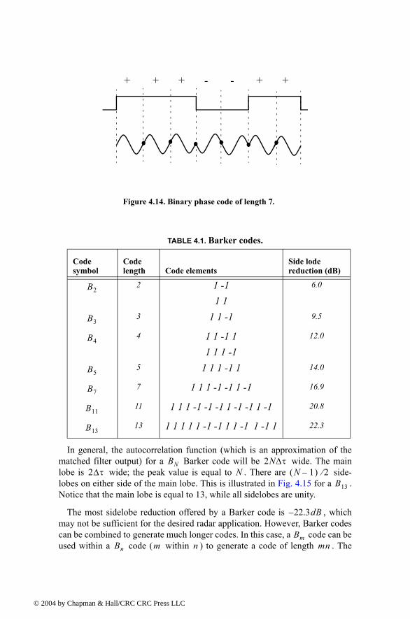
© 200
In general, the autocorrelation function (which is an approximation of the matched filter output) for a Barker code will be wide. The main lobe is wide; the peak value is equal to . There are side-lobes on either side of the main lobe. This is illustrated in Fig. 4.15 for a . Notice that the main lobe is equal to 13, while all sidelobes are unity.
The most sidelobe reduction offered by a Barker code is , which may not be sufficient for the desired radar application. However, Barker codes can be combined to generate much longer codes. In this case, a code can be used within a code ( within ) to generate a code of length . The
TABLE 4.1. Barker codes.
Code symbol
Code length Code elements
Side lode reduction (dB)
2 1 -11 1
6.0
3 1 1 -1 9.5
4 1 1 -1 11 1 1 -1
12.0
5 1 1 1 -1 1 14.0
7 1 1 1 -1 -1 1 -1 16.9
11 1 1 1 -1 -1 -1 1 -1 -1 1 -1 20.8
13 1 1 1 1 1 -1 -1 1 1 -1 1 -1 1 22.3
+ + + - - + +
Figure 4.14. Binary phase code of length 7.
B2
B3
B4
B5
B7
B11
B13
BN 2N∆τ2∆τ N N 1( ) 2⁄
B13
22.3dB
BmBn m n mn
4 by Chapman & Hall/CRC CRC Press LLC
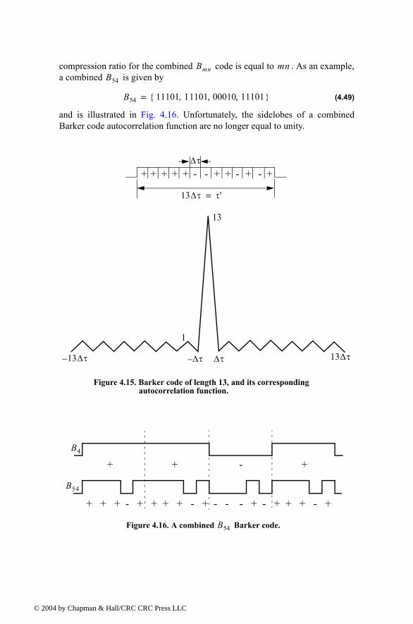
© 200
compression ratio for the combined code is equal to . As an example, a combined is given by
(4.49)
and is illustrated in Fig. 4.16. Unfortunately, the sidelobes of a combined Barker code autocorrelation function are no longer equal to unity.
Bmn mnB54
B54 11101 11101 00010 11101, , , =
+ + + + + - - + + - + - +
13∆τ τ'=
∆τ
1
13
∆τ∆τ 13∆τ13 ∆τ
Figure 4.15. Barker code of length 13, and its corresponding autocorrelation function.
+ + + - + + + + - + - - - + - + + + - +
B4
+ + - +
B54
Figure 4.16. A combined Barker code.B54
4 by Chapman & Hall/CRC CRC Press LLC
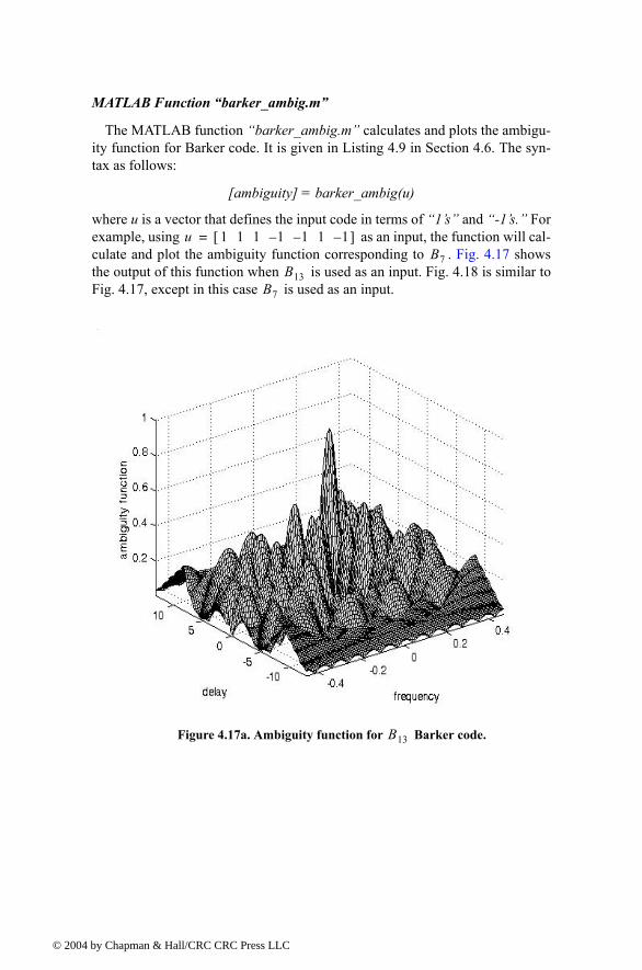
© 200
MATLAB Function barker_ambig.m
The MATLAB function barker_ambig.m calculates and plots the ambigu-ity function for Barker code. It is given in Listing 4.9 in Section 4.6. The syn-tax as follows:
[ambiguity] = barker_ambig(u)
where u is a vector that defines the input code in terms of 1s and -1s. For example, using as an input, the function will cal-culate and plot the ambiguity function corresponding to . Fig. 4.17 shows the output of this function when is used as an input. Fig. 4.18 is similar to Fig. 4.17, except in this case is used as an input.
u 1 1 1 1 1 1 1[ ]=B7
B13B7
Figure 4.17a. Ambiguity function for Barker code.B13
4 by Chapman & Hall/CRC CRC Press LLC
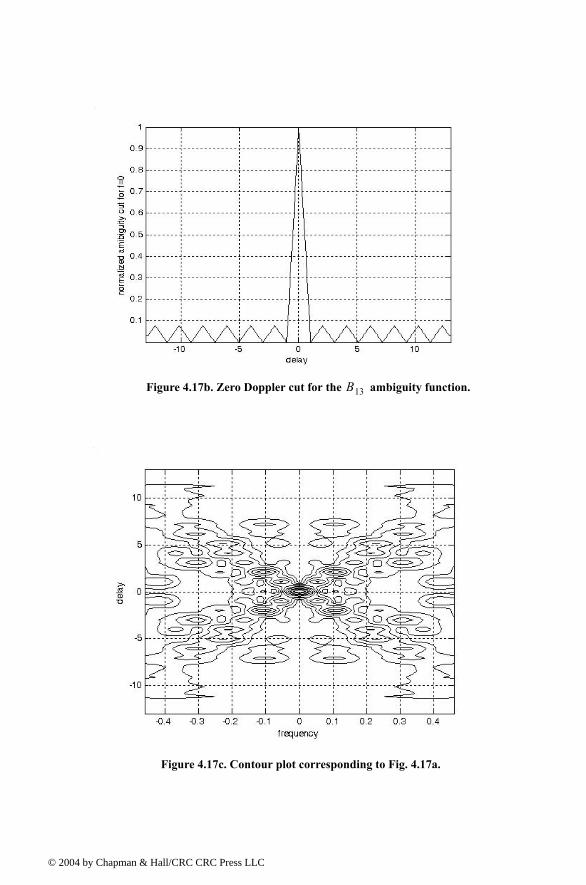
© 200
Figure 4.17b. Zero Doppler cut for the ambiguity function.B13
Figure 4.17c. Contour plot corresponding to Fig. 4.17a.
4 by Chapman & Hall/CRC CRC Press LLC
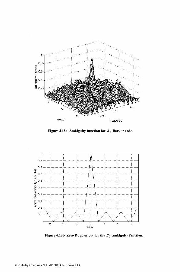
© 200
Figure 4.18a. Ambiguity function for Barker code.B7
Figure 4.18b. Zero Doppler cut for the ambiguity function.B7
4 by Chapman & Hall/CRC CRC Press LLC
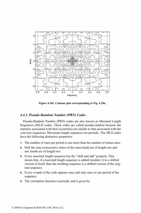
© 200
4.4.3. Pseudo-Random Number (PRN) Codes
Pseudo-Random Number (PRN) codes are also known as Maximal Length Sequences (MLS) codes. These codes are called pseudo-random because the statistics associated with their occurrence are similar to that associated with the coin-toss sequences. Maximum length sequences are periodic. The MLS codes have the following distinctive properties:
1. The number of ones per period is one more than the number of minus-ones.2. Half the runs (consecutive states of the same kind) are of length one and
one fourth are of length two.3. Every maximal length sequence has the shift and add property. This
means that, if a maximal length sequence is added (modulo 2) to a shifted version of itself, then the resulting sequence is a shifted version of the orig-inal sequence.
4. Every n-tuple of the code appears once and only once in one period of the sequence.
5. The correlation function is periodic and is given by
Figure 4.18c. Contour plot corresponding to Fig. 4.18a.
4 by Chapman & Hall/CRC CRC Press LLC
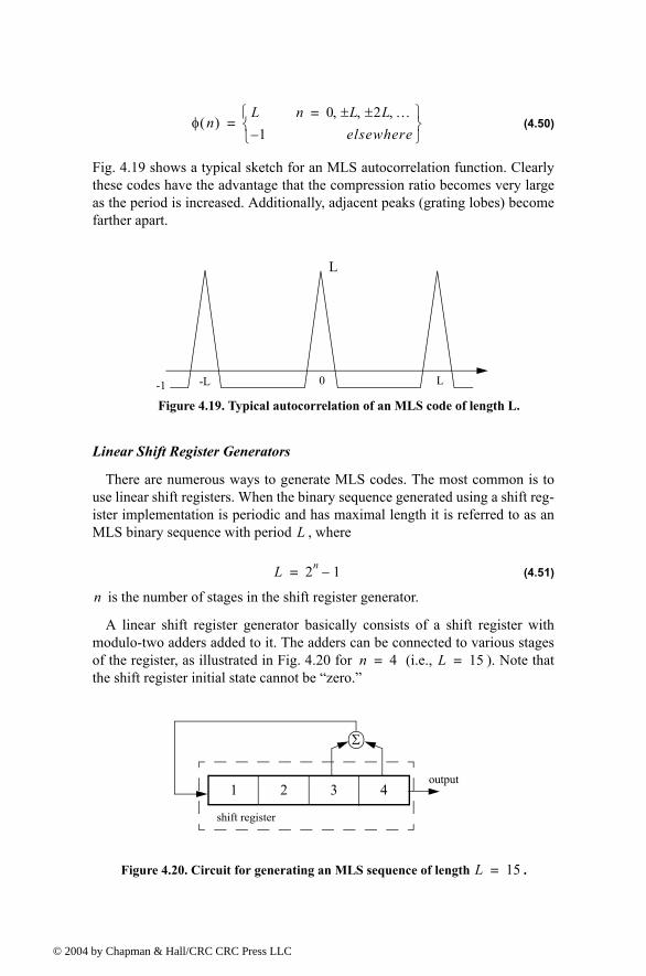
© 200
(4.50)
Fig. 4.19 shows a typical sketch for an MLS autocorrelation function. Clearly these codes have the advantage that the compression ratio becomes very large as the period is increased. Additionally, adjacent peaks (grating lobes) become farther apart.
Linear Shift Register Generators
There are numerous ways to generate MLS codes. The most common is to use linear shift registers. When the binary sequence generated using a shift reg-ister implementation is periodic and has maximal length it is referred to as an MLS binary sequence with period , where
(4.51)
is the number of stages in the shift register generator.
A linear shift register generator basically consists of a shift register with modulo-two adders added to it. The adders can be connected to various stages of the register, as illustrated in Fig. 4.20 for (i.e., ). Note that the shift register initial state cannot be zero.
φ n( )L n 0 L 2L …,±,±,=
1 elsewhere
=
L-L 0-1
L
Figure 4.19. Typical autocorrelation of an MLS code of length L.
L
L 2n 1=
n
n 4= L 15=
Σ
Figure 4.20. Circuit for generating an MLS sequence of length .L 15=
1 2 3 4
shift register
output
4 by Chapman & Hall/CRC CRC Press LLC
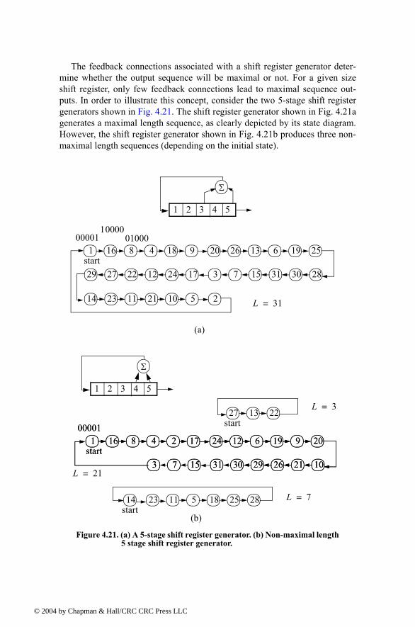
© 200
The feedback connections associated with a shift register generator deter-mine whether the output sequence will be maximal or not. For a given size shift register, only few feedback connections lead to maximal sequence out-puts. In order to illustrate this concept, consider the two 5-stage shift register generators shown in Fig. 4.21. The shift register generator shown in Fig. 4.21a generates a maximal length sequence, as clearly depicted by its state diagram. However, the shift register generator shown in Fig. 4.21b produces three non-maximal length sequences (depending on the initial state).
1 2 3 4 5
Σ
start
0000116 48 9181 26 613 251920
27 1222 172429 7 3115 28303
23 2111 51014 2
1000001000
1 2 3 4 5
Σ
(a)
start
0000116 48 1721 12 196 20924
3 157 30 2629 102131
L 31=
start
0000116 48 1721 12 196 20924
3 157 30 2629 102131
27 2213
14 11 185 282523
L 21=
L 3=
L 7=
Figure 4.21. (a) A 5-stage shift register generator. (b) Non-maximal length 5 stage shift register generator.
(b)
start
start
4 by Chapman & Hall/CRC CRC Press LLC
© 200
Given an n-stage shift register generator, one would be interested in knowing how many feedback connections will yield maximal length sequences. Zierler1
showed that the number of maximal length sequences possible for a given n-stage linear shift register generator is given by
(4.52)
where is the Eulers totient (or Eulers phi) function. Eulers phi function is defined by
(4.53)
where are the prime factors of . Note that when has multiples, then only one of them is used (see example in Eq. (4.56)). Also note that when is a prime number, then the Eulers phi function is
(4.54)
For example, a 3-stage shift register generator will produce
(4.55)
and a 6-stage shift register,
(4.56)
Maximal Length Sequence Characteristic Polynomial
Consider an n-stage maximal length linear shift register whose feedback connections correspond to . This maximal length shift register can be described using its characteristic polynomial defined by
(4.57)
where the additions are modulo 2. Therefore, if the characteristic polynomial for an n-stage shift register is known, one can easily determine the register feedback connections and consequently deduce the corresponding maximal length sequence. For example, consider a 6-stage shift register whose charac-teristic polynomial is
1. Zierler, N., Several Binary-Sequence Generators, MIT Technical Report No. 95, Sept. 1955.
NLϕ 2n 1( )
n-----------------------=
ϕ
ϕ k( ) kpi 1( )
pi------------------
i∏=
pi k pik
ϕ k( ) k 1=
NLϕ 23 1( )
3----------------------- ϕ 7( )
3----------- 7 1
3------------ 2= = = =
NLϕ 26 1( )
6----------------------- ϕ 63( )
6-------------- 63
6------ 3 1( )
3---------------- 7 1( )
7----------------×× 6= = = =
n k m etc, , ,
xn xk xm … 1+ + + +
4 by Chapman & Hall/CRC CRC Press LLC
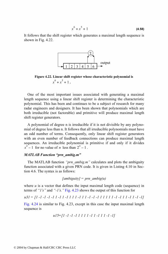
© 200
(4.58)
It follows that the shift register which generates a maximal length sequence is shown in Fig. 4.22.
One of the most important issues associated with generating a maximal length sequence using a linear shift register is determining the characteristic polynomial. This has been and continues to be a subject of research for many radar engineers and designers. It has been shown that polynomials which are both irreducible (not factorable) and primitive will produce maximal length shift register generators.
A polynomial of degree n is irreducible if it is not divisible by any polyno-mial of degree less than n. It follows that all irreducible polynomials must have an odd number of terms. Consequently, only linear shift register generators with an even number of feedback connections can produce maximal length sequences. An irreducible polynomial is primitive if and only if it divides
for no value of less than .
MATLAB Function prn_ambig.m
The MATLAB function prn_ambig.m calculates and plots the ambiguity function associated with a given PRN code. It is given in Listing 4.10 in Sec-tion 4.6. The syntax is as follows:
[ambiguity] = prn_ambig(u)
where u is a vector that defines the input maximal length code (sequence) in terms of 1s and -1s. Fig. 4.23 shows the output of this function for
u31 = [1 -1 -1 -1 -1 1 -1 1 -1 1 1 1 -1 1 1 -1 -1 -1 1 1 1 1 1 -1 -1 1 1 -1 1 -1 -1]
Fig. 4.24 is similar to Fig. 4.23, except in this case the input maximal length sequence is
u15=[1 -1 -1 -1 1 1 1 1 -1 1 -1 1 1 -1 -1]
x6 x5 1+ +
1 2 3 4 5 6
Σ
output
Figure 4.22. Linear shift register whose characteristic polynomial is
.x6 x5 1+ +
xn 1 n 2n 1
4 by Chapman & Hall/CRC CRC Press LLC
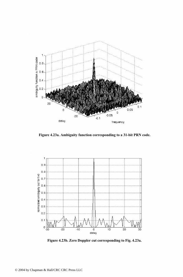
© 200
Figure 4.23a. Ambiguity function corresponding to a 31-bit PRN code.
Figure 4.23b. Zero Doppler cut corresponding to Fig. 4.23a.
4 by Chapman & Hall/CRC CRC Press LLC
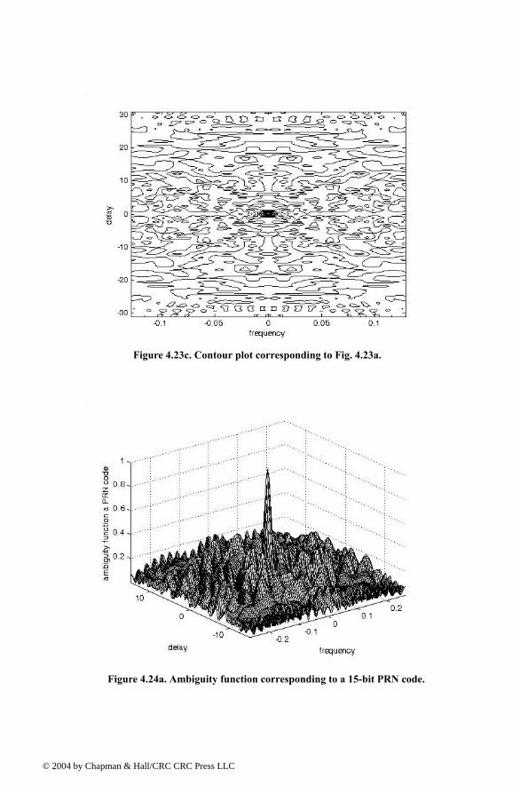
© 200
Figure 4.23c. Contour plot corresponding to Fig. 4.23a.
Figure 4.24a. Ambiguity function corresponding to a 15-bit PRN code.
4 by Chapman & Hall/CRC CRC Press LLC
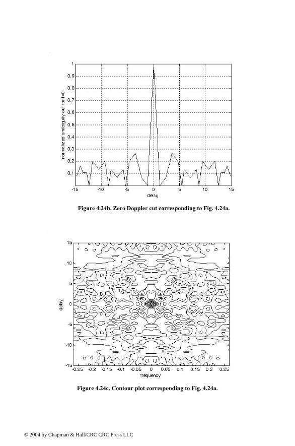
© 200
Figure 4.24b. Zero Doppler cut corresponding to Fig. 4.24a.
Figure 4.24c. Contour plot corresponding to Fig. 4.24a.
4 by Chapman & Hall/CRC CRC Press LLC
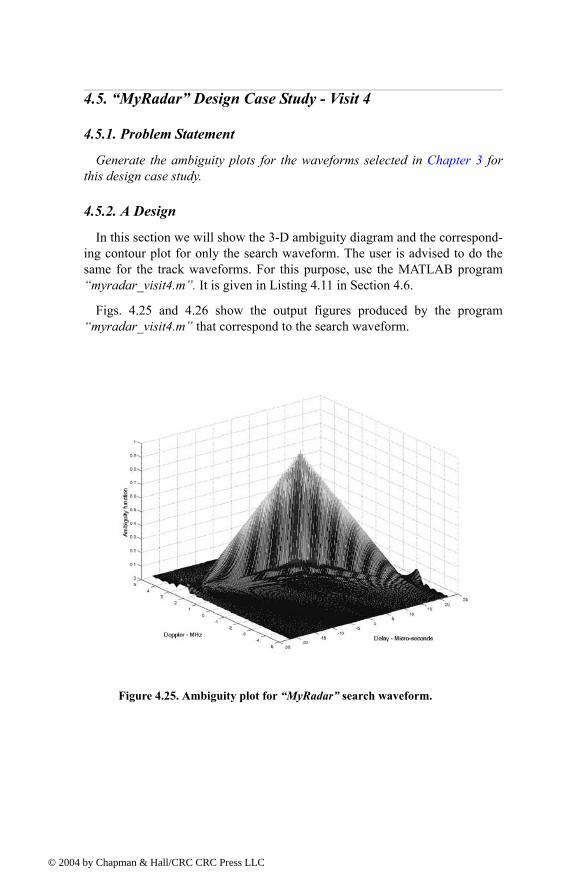
© 200
4.5. MyRadar Design Case Study - Visit 4
4.5.1. Problem Statement
Generate the ambiguity plots for the waveforms selected in Chapter 3 for this design case study.
4.5.2. A Design
In this section we will show the 3-D ambiguity diagram and the correspond-ing contour plot for only the search waveform. The user is advised to do the same for the track waveforms. For this purpose, use the MATLAB program myradar_visit4.m. It is given in Listing 4.11 in Section 4.6.
Figs. 4.25 and 4.26 show the output figures produced by the program myradar_visit4.m that correspond to the search waveform.
Figure 4.25. Ambiguity plot for MyRadar search waveform.
4 by Chapman & Hall/CRC CRC Press LLC
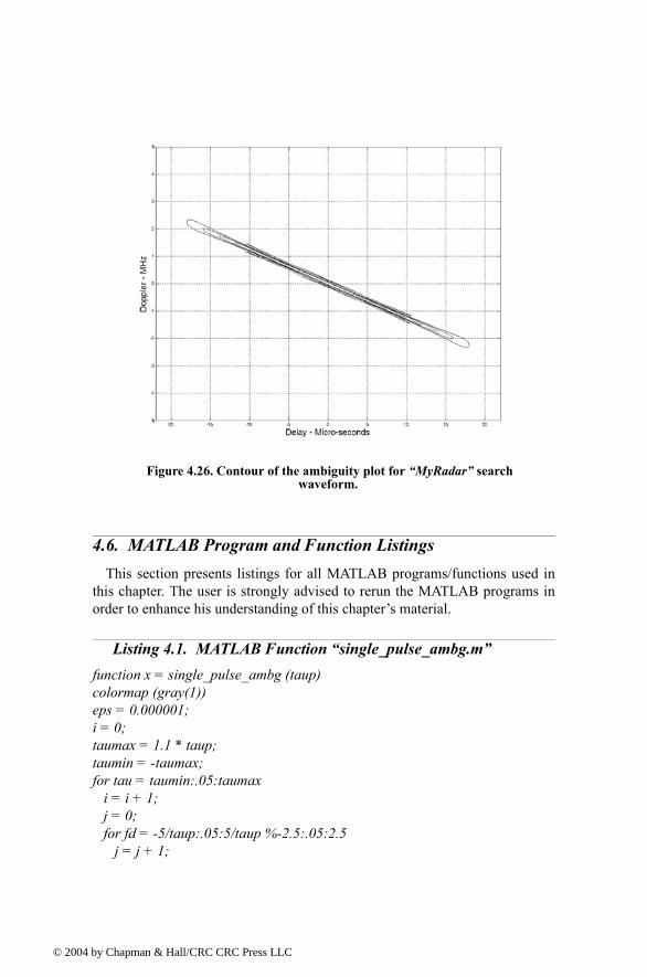
© 200
4.6. MATLAB Program and Function ListingsThis section presents listings for all MATLAB programs/functions used in
this chapter. The user is strongly advised to rerun the MATLAB programs in order to enhance his understanding of this chapters material.
Listing 4.1. MATLAB Function single_pulse_ambg.mfunction x = single_pulse_ambg (taup)colormap (gray(1))eps = 0.000001;i = 0;taumax = 1.1 * taup;taumin = -taumax;for tau = taumin:.05:taumax i = i + 1; j = 0; for fd = -5/taup:.05:5/taup %-2.5:.05:2.5 j = j + 1;
Figure 4.26. Contour of the ambiguity plot for MyRadar search waveform.
4 by Chapman & Hall/CRC CRC Press LLC
© 200
val1 = 1. - abs(tau) / taup; val2 = pi * taup * (1.0 - abs(tau) / taup) * fd; x(j,i) = abs( val1 * sin(val2+eps)/(val2+eps)); endend
Listing 4.2. MATLAB Program fig4_2.m% Use this program to reproduce Fig. 4.2 of textclose allclear alleps = 0.000001;taup = 2.;taumin = -1.1 * taup;taumax = -taumin;x = single_pulse_ambg(taup);taux = taumin:.05:taumax;fdy = -5/taup:.05:5/taup;figure(1)mesh(taux,fdy,x);xlabel ('Delay - seconds')ylabel ('Doppler - Hz')zlabel ('Ambiguity function')colormap([.5 .5 .5])colormap (gray)figure(2)contour(taux,fdy,x);xlabel ('Delay - seconds')ylabel ('Doppler - Hz')colormap([.5 .5 .5])colormap (gray)gridy = x.^2;figure(3)mesh(taux,fdy,y);xlabel ('Delay - seconds')ylabel ('Doppler - Hz')zlabel ('Ambiguity function')colormap([.5 .5 .5])colormap (gray)figure(4)contour(taux,fdy,y);xlabel ('Delay - seconds')ylabel ('Doppler - Hz')
4 by Chapman & Hall/CRC CRC Press LLC
© 200
colormap([.5 .5 .5])colormap (gray)grid
Listing 4.3. MATLAB Program fig4_4.m% Use this program to reproduce Fig 4.4 of textclose allclear alleps = 0.0001;taup = 2.;fd = -10./taup:.05:10./taup;uncer = abs( sinc(taup .* fd));ambg = uncer.^2;plot(fd, ambg,'k')xlabel ('Frequency - Hz')ylabel ('Ambiguity - Volts')gridfigure(2)plot (fd, uncer,'k');xlabel ('Frequency - Hz')ylabel ('Uncertainty - Volts')grid
Listing 4.4. MATLAB Function lfm_ambg.mffunction x = lfm_ambg(taup, b, up_down)eps = 0.000001;i = 0;mu = up_down * b / 2. / taup;delt = 2.2*taup/250;delf = 2*b /250;for tau = -1.1*taup:.05:1.1*taup i = i + 1; j = 0; for fd = -b:.05:b j = j + 1; val1 = 1. - abs(tau) / taup; val2 = pi * taup * (1.0 - abs(tau) / taup); val3 = (fd + mu * tau); val = val2 * val3; x(j,i) = abs( val1 * (sin(val+eps)/(val+eps))).^2; endend
4 by Chapman & Hall/CRC CRC Press LLC
© 200
Listing 4.5. MATLAB Program fig4_5.m% Use this program to reproduce Fig. 4.5 of textclose allclear alleps = 0.0001;taup = 1.;b =10.;up_down = 1.;x = lfm_ambg(taup, b, up_down);taux = -1.1*taup:.05:1.1*taup;fdy = -b:.05:b;figure(1)mesh(taux,fdy,x)xlabel ('Delay - seconds')ylabel ('Doppler - Hz')zlabel ('Ambiguity function')figure(2)contour(taux,fdy,x)xlabel ('Delay - seconds')ylabel ('Doppler - Hz')y = sqrt(x);figure(3)mesh(taux,fdy,y)xlabel ('Delay - seconds')ylabel ('Doppler - Hz')zlabel ('Uncertainty function')figure(4)contour(taux,fdy,y)xlabel ('Delay - seconds')ylabel ('Doppler - Hz')
Listing 4.6. MATLAB Program fig4_6.m% Use this program to reproduce Fig. 4.6 of textclose allclear alltaup = 1;b =20.;up_down = 1.;taux = -1.5*taup:.01:1.5*taup;fd = 0.;mu = up_down * b / 2. / taup;ii = 0.;
4 by Chapman & Hall/CRC CRC Press LLC
© 200
for tau = -1.5*taup:.01:1.5*taup ii = ii + 1; val1 = 1. - abs(tau) / taup; val2 = pi * taup * (1.0 - abs(tau) / taup); val3 = (fd + mu * tau); val = val2 * val3; x(ii) = abs( val1 * (sin(val+eps)/(val+eps)));endfigure(1)plot(taux,x)gridxlabel ('Delay - seconds')ylabel ('Uncertainty')figure(2)plot(taux,x.^2)gridxlabel ('Delay - seconds')ylabel ('Ambiguity')
Listing 4.7. MATLAB Function train_ambg.mfunction x = train_ambg (taup, n, pri)if( taup > pri / 2.) 'ERROR. Pulsewidth must be less than the PRI/2.' returnendgap = pri - 2.*taup;eps = 0.000001;b = 1. / taup;ii = 0.;for q = -(n-1):1:n-1 tauo = q - taup ; index = -1.; for tau1 = tauo:0.0533:tauo+gap+2.*taup index = index + 1; tau = -taup + index*.0533; ii = ii + 1; j = 0.; for fd = -b:.0533:b j = j + 1; if (abs(tau) <= taup) val1 = 1. -abs(tau) / taup; val2 = pi * taup * fd * (1.0 - abs(tau) / taup); val3 = abs(val1 * sin(val2+eps) /(val2+eps));
4 by Chapman & Hall/CRC CRC Press LLC
© 200
val4 = abs((sin(pi*fd*(n-abs(q))*pri+eps))/(sin(pi*fd*pri+eps))); x(j,ii)= val3 * val4 / n; else x(j,ii) = 0.; end end endend
Listing 4.8. MATLAB Program fig4_8.m% Use this program to reproduce Fig. 4.8 of textclose allclear alltaup =0.2;pri=1;n=5;x = train_ambg (taup, n, pri);figure(1)mesh(x)xlabel ('Delay - seconds')ylabel ('Doppler - Hz')zlabel ('Ambiguity function')figure(2)contour(x);xlabel ('Delay - seconds')ylabel ('Doppler - Hz')
Listing 4.9. MATLAB Function barker_ambig.mfunction [ambig] = barker_ambig(uinput)% Compute and plot the ambiguity function for a Barker code%Compute the ambiguity function% by utilizing the FFT through combining multiple range cutsN = size(uinput,2);tau = N;Barker_code = uinput;samp_num = size(Barker_code,2) *10;n = ceil(log(samp_num) / log(2));nfft = 2^n;u(1:nfft) = 0;j = 0;for index = 1:10:samp_num index;
4 by Chapman & Hall/CRC CRC Press LLC

© 200
j = j+1; u(index:index+10-1) = Barker_code(j);endv = u;delay = linspace(-tau, tau, nfft);freq_del = 12 / tau /100;j = 0;vfft = fft(v,nfft);for freq = -6/tau:freq_del:6/tau; j = j+1; exf = exp(sqrt(-1) * 2. * pi * freq .* delay); u_times_exf = u .* exf; ufft = fft(u_times_exf,nfft); prod = ufft .* conj(vfft); ambig(:,j) = fftshift(abs(ifft(prod))');endfreq = -6/tau:freq_del:6/tau;delay = linspace(-N,N,nfft);figure (1)mesh(freq,delay,ambig ./ max(max(ambig)))colormap([.5 .5 .5])colormap(gray)axis tightxlabel('frequency')ylabel('delay')zlabel('ambiguity function')figure (2)value = 10 * N ;plot(delay,ambig(:,51)/value,'k')xlabel('delay')ylabel('normalized amibiguity cut for f=0')gridaxis tightfigure (3)contour(freq,delay,ambig ./ max(max(ambig)))colormap([.5 .5 .5])colormap (gray)xlabel('frequency')ylabel('delay')grid on
Listing 4.10. MATLAB Function prn_ambig.mfunction [ambig] = prn_ambig(uinput)
4 by Chapman & Hall/CRC CRC Press LLC
© 200
% Compute and plot the ambiguity function for a PRN code% Compute the ambiguity function by utilizing the FFT % through combining multiple range cuts
N = size(uinput,2);tau = N;PRN = uinput;samp_num = size(PRN,2) * 10;n = ceil(log(samp_num) / log(2));nfft = 2^n;u(1:nfft) = 0;j = 0;for index = 1:10:samp_num index; j = j+1; u(index:index+10-1) = PRN(j);end% set-up the array vv = u;delay = linspace(0,5*tau,nfft);freq_del = 8 / tau /100;j = 0;vfft = fft(v,nfft);for freq = -4/tau:freq_del:4/tau; j = j+1; exf = exp(sqrt(-1) * 2. * pi * freq .* delay); u_times_exf = u .* exf; ufft = fft(u_times_exf,nfft); prod = ufft .* conj(vfft); ambig(:,j) = fftshift(abs(ifft(prod))');endfreq = -4/tau:freq_del:4/tau;delay = linspace(-N,N,nfft);figure(1)mesh(freq,delay,ambig ./ max(max(ambig)))colormap([.5 .5 .5])colormap(gray)axis tightxlabel('frequency')ylabel('delay')zlabel('ambiguity function a PRN code')figure(2)plot(delay,ambig(:,51)/(max(max(ambig))),'k')xlabel('delay')
4 by Chapman & Hall/CRC CRC Press LLC
© 200
ylabel('normalized amibiguity cut for f=0')gridaxis tightfigure(3)contour(freq,delay,ambig ./ max(max(ambig)))axis tightcolormap([.5 .5 .5])colormap(gray)xlabel('frequency')ylabel('delay')
Listing 4.11. MATLAB Program myradar_visit4.m% Use this program to reproduce Figs. 4.25 to 4.27 of the textclose allclear alleps = 0.0001;taup = 20.e-6;b =1.e6;up_down = 1.;i = 0;mu = up_down * b / 2. / taup;delt = 2.2*taup /250;delf = 2*b /300;for tau = -1.1*taup:delt:1.1*taup i = i + 1; j = 0; for fd = -b:delf:b j = j + 1; val1 = 1. - abs(tau) / taup; val2 = pi * taup * (1.0 - abs(tau) / taup); val3 = (fd + mu * tau); val = val2 * val3; x(j,i) = abs( val1 * (sin(val+eps)/(val+eps))).^2; endendtaux = linspace(-1.1*taup,1.1*taup,251).*1e6;fdy = linspace(-b,b,301) .* 1e-6;figure(1)mesh(taux,fdy,sqrt(x))xlabel ('Delay - Micro-seconds')ylabel ('Doppler - MHz')zlabel ('Ambiguity function')figure(2)
4 by Chapman & Hall/CRC CRC Press LLC

© 200
contour(taux,fdy,sqrt(x))xlabel ('Delay - Micro-seconds')ylabel ('Doppler - MHz')grid
4 by Chapman & Hall/CRC CRC Press LLC
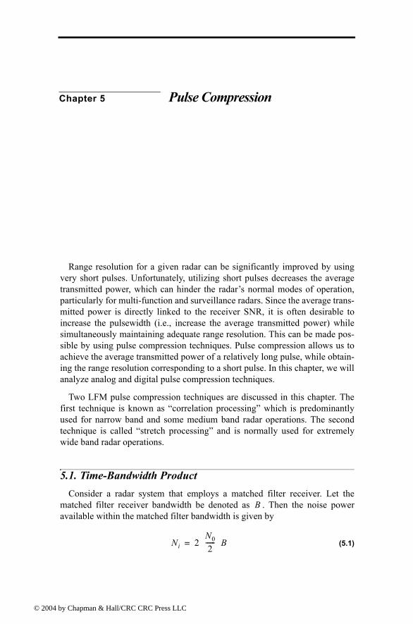
© 200
Chapter 5 Pulse Compression
Range resolution for a given radar can be significantly improved by using very short pulses. Unfortunately, utilizing short pulses decreases the average transmitted power, which can hinder the radars normal modes of operation, particularly for multi-function and surveillance radars. Since the average trans-mitted power is directly linked to the receiver SNR, it is often desirable to increase the pulsewidth (i.e., increase the average transmitted power) while simultaneously maintaining adequate range resolution. This can be made pos-sible by using pulse compression techniques. Pulse compression allows us to achieve the average transmitted power of a relatively long pulse, while obtain-ing the range resolution corresponding to a short pulse. In this chapter, we will analyze analog and digital pulse compression techniques.
Two LFM pulse compression techniques are discussed in this chapter. The first technique is known as correlation processing which is predominantly used for narrow band and some medium band radar operations. The second technique is called stretch processing and is normally used for extremely wide band radar operations.
5.1. Time-Bandwidth ProductConsider a radar system that employs a matched filter receiver. Let the
matched filter receiver bandwidth be denoted as . Then the noise power available within the matched filter bandwidth is given by
(5.1)
B
Ni 2N0
2------ B=
4 by Chapman & Hall/CRC CRC Press LLC
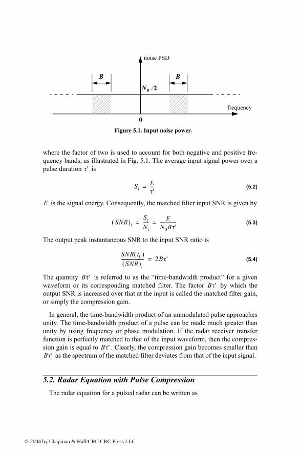
© 200
where the factor of two is used to account for both negative and positive fre-quency bands, as illustrated in Fig. 5.1. The average input signal power over a pulse duration is
(5.2)
is the signal energy. Consequently, the matched filter input SNR is given by
(5.3)
The output peak instantaneous SNR to the input SNR ratio is
(5.4)
The quantity is referred to as the time-bandwidth product for a given waveform or its corresponding matched filter. The factor by which the output SNR is increased over that at the input is called the matched filter gain, or simply the compression gain.
In general, the time-bandwidth product of an unmodulated pulse approaches unity. The time-bandwidth product of a pulse can be made much greater than unity by using frequency or phase modulation. If the radar receiver transfer function is perfectly matched to that of the input waveform, then the compres-sion gain is equal to . Clearly, the compression gain becomes smaller than
as the spectrum of the matched filter deviates from that of the input signal.
5.2. Radar Equation with Pulse CompressionThe radar equation for a pulsed radar can be written as
B B
N0 2⁄
0
noise PSD
frequency
Figure 5.1. Input noise power.
τ'
SiEτ'---=
E
SNR( )iSi
Ni----- E
N0Bτ'--------------= =
SNR t0( )SNR( )i
-------------------- 2Bτ'=
Bτ'Bτ'
Bτ'Bτ'
4 by Chapman & Hall/CRC CRC Press LLC
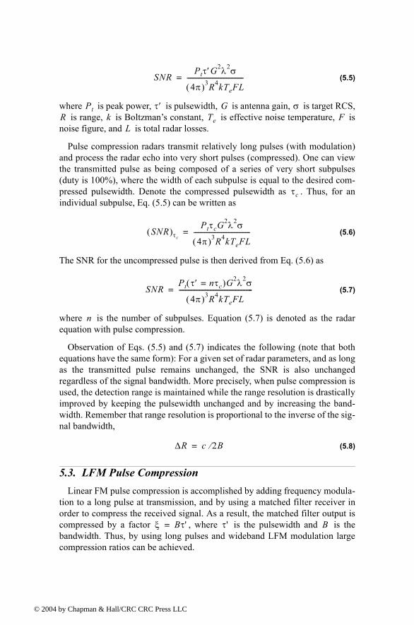
© 200
(5.5)
where is peak power, is pulsewidth, is antenna gain, is target RCS, is range, is Boltzmans constant, is effective noise temperature, is
noise figure, and is total radar losses.
Pulse compression radars transmit relatively long pulses (with modulation) and process the radar echo into very short pulses (compressed). One can view the transmitted pulse as being composed of a series of very short subpulses (duty is 100%), where the width of each subpulse is equal to the desired com-pressed pulsewidth. Denote the compressed pulsewidth as . Thus, for an individual subpulse, Eq. (5.5) can be written as
(5.6)
The SNR for the uncompressed pulse is then derived from Eq. (5.6) as
(5.7)
where is the number of subpulses. Equation (5.7) is denoted as the radar equation with pulse compression.
Observation of Eqs. (5.5) and (5.7) indicates the following (note that both equations have the same form): For a given set of radar parameters, and as long as the transmitted pulse remains unchanged, the SNR is also unchanged regardless of the signal bandwidth. More precisely, when pulse compression is used, the detection range is maintained while the range resolution is drastically improved by keeping the pulsewidth unchanged and by increasing the band-width. Remember that range resolution is proportional to the inverse of the sig-nal bandwidth,
(5.8)
5.3. LFM Pulse CompressionLinear FM pulse compression is accomplished by adding frequency modula-
tion to a long pulse at transmission, and by using a matched filter receiver in order to compress the received signal. As a result, the matched filter output is compressed by a factor , where is the pulsewidth and is the bandwidth. Thus, by using long pulses and wideband LFM modulation large compression ratios can be achieved.
SNRPtτ′G
2λ2σ
4π( )3R4kTeFL------------------------------------=
Pt τ′ G σR k Te F
L
τc
SNR( )τc
PtτcG2λ2σ
4π( )3R4kTeFL------------------------------------=
SNRPt τ′ nτc=( )G2λ2σ
4π( )3R4kTeFL-----------------------------------------------=
n
∆R c 2B⁄=
ξ Bτ'= τ' B
4 by Chapman & Hall/CRC CRC Press LLC
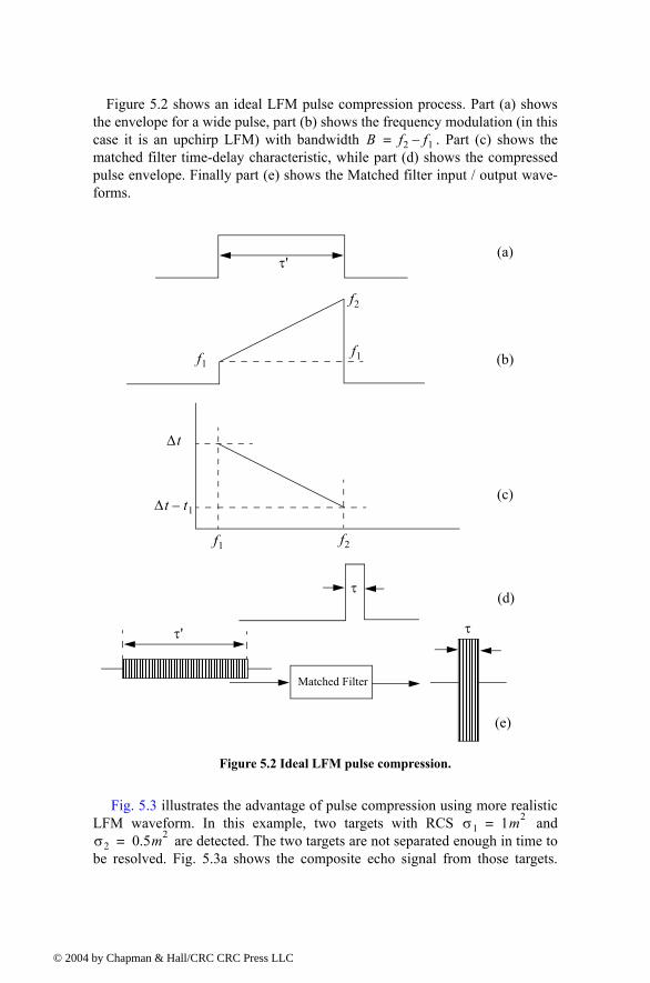
© 200
Figure 5.2 shows an ideal LFM pulse compression process. Part (a) shows the envelope for a wide pulse, part (b) shows the frequency modulation (in this case it is an upchirp LFM) with bandwidth . Part (c) shows the matched filter time-delay characteristic, while part (d) shows the compressed pulse envelope. Finally part (e) shows the Matched filter input / output wave-forms.
Fig. 5.3 illustrates the advantage of pulse compression using more realistic LFM waveform. In this example, two targets with RCS and
are detected. The two targets are not separated enough in time to be resolved. Fig. 5.3a shows the composite echo signal from those targets.
B f2 f1=
(a)
(b)
(c)
(d)
(e)
Matched Filter
τ'
f2
f1
∆t
∆t t1
f1 f2
τ
τ' τ
Figure 5.2 Ideal LFM pulse compression.
f1
σ1 1m2=σ2 0.5m2=
4 by Chapman & Hall/CRC CRC Press LLC
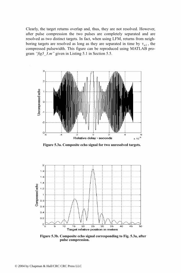
© 200
Clearly, the target returns overlap and, thus, they are not resolved. However, after pulse compression the two pulses are completely separated and are resolved as two distinct targets. In fact, when using LFM, returns from neigh-boring targets are resolved as long as they are separated in time by , the compressed pulsewidth. This figure can be reproduced using MATLAB pro-gram fig5_3.m given in Listing 5.1 in Section 5.5.
τn1
Figure 5.3a. Composite echo signal for two unresolved targets.
Figure 5.3b. Composite echo signal corresponding to Fig. 5.3a, after pulse compression.
4 by Chapman & Hall/CRC CRC Press LLC
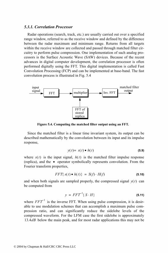
© 200
5.3.1. Correlation Processor
Radar operations (search, track, etc.) are usually carried out over a specified range window, referred to as the receive window and defined by the difference between the radar maximum and minimum range. Returns from all targets within the receive window are collected and passed through matched filter cir-cuitry to perform pulse compression. One implementation of such analog pro-cessors is the Surface Acoustic Wave (SAW) devices. Because of the recent advances in digital computer development, the correlation processor is often performed digitally using the FFT. This digital implementation is called Fast Convolution Processing (FCP) and can be implemented at base-band. The fast convolution process is illustrated in Fig. 5.4
Since the matched filter is a linear time invariant system, its output can be described mathematically by the convolution between its input and its impulse response,
(5.9)
where is the input signal, is the matched filter impulse response (replica), and the operator symbolically represents convolution. From the Fourier transform properties,
(5.10)
and when both signals are sampled properly, the compressed signal can be computed from
(5.11)
where is the inverse FFT. When using pulse compression, it is desir-able to use modulation schemes that can accomplish a maximum pulse com-pression ratio, and can significantly reduce the sidelobe levels of the compressed waveform. For the LFM case the first sidelobe is approximately
below the main peak, and for most radar applications this may not be
FFT multiplier
FFT of
Inv. FFTinputsignal
matched filter output
Figure 5.4. Computing the matched filter output using an FFT.
storedreplica
y t( ) s t( ) h t( )•=
s t( ) h t( )•
FFT s t( ) h t( )• S f( ) H f( )⋅=
y t( )
y FFT 1 S H⋅ =
FFT 1
13.4dB
4 by Chapman & Hall/CRC CRC Press LLC
© 200
sufficient. In practice, high sidelobe levels are not preferable because noise and/or jammers located at the sidelobes may interfere with target returns in the main lobe.
Weighting functions (windows) can be used on the compressed pulse spec-trum in order to reduce the sidelobe levels. The cost associated with such an approach is a loss in the main lobe resolution, and a reduction in the peak value (i.e., loss in the SNR). Weighting the time domain transmitted or received sig-nal instead of the compressed pulse spectrum will theoretically achieve the same goal. However, this approach is rarely used, since amplitude modulating the transmitted waveform introduces extra burdens on the transmitter.
Consider a radar system that utilizes a correlation processor receiver (i.e., matched filter). The receive window in meters is defined by
(5.12)
where and , respectively, define the maximum and minimum range over which the radar performs detection. Typically is limited to the extent of the target complex. The normalized complex transmitted signal has the form
(5.13)
is the pulsewidth, , and is the bandwidth.
The radar echo signal is similar to the transmitted one with the exception of a time delay and an amplitude change that correspond to the target RCS. Con-sider a target at range . The echo received by the radar from this target is
(5.14)
where is proportional to target RCS, antenna gain, and range attenuation. The time delay is given by
(5.15)
The first step of the processing consists of removing the frequency . This is accomplished by mixing with a reference signal whose phase is . The phase of the resultant signal, after low pass filtering, is then given by
(5.16)
and the instantaneous frequency is
(5.17)
Rrec Rmax Rmin=
Rmax RminRrec
s t( ) j2π f0t µ2---t2+
exp= 0 t τ′≤ ≤
τ′ µ B τ′⁄= B
R1
sr t( ) a1 j2π f0 t τ1( ) µ2--- t τ1( )2+
exp=
a1τ1
τ1 2R1 c⁄=
f0sr t( ) 2πf0t
ψ t( ) 2π f 0τ1µ2--- t τ1( )2+
=
fi t( ) 12π------
tdd ψ t( ) µ t τ1( ) B
τ′---- t
2R1
c---------
= = =
4 by Chapman & Hall/CRC CRC Press LLC
© 200
The quadrature components are
(5.18)
Sampling the quadrature components is performed next. The number of sam-ples, , must be chosen so that foldover (ambiguity) in the spectrum is avoided. For this purpose, the sampling frequency, (based on the Nyquist sampling rate), must be
(5.19)
and the sampling interval is
(5.20)
Using Eq. (5.17) it can be shown that (the proof is left as an exercise) the fre-quency resolution of the FFT is
(5.21)
The minimum required number of samples is
(5.22)
Equating Eqs. (5.20) and (5.22) yields
(5.23)
Consequently, a total of real samples, or complex samples, is suf-ficient to completely describe an LFM waveform of duration and bandwidth
. For example, an LFM signal of duration and bandwidth requires 200 real samples to determine the input signal (100
samples for the I-channel and 100 samples for the Q-channel).
For better implementation of the FFT is extended to the next power of two, by zero padding. Thus, the total number of samples, for some positive integer , is
(5.24)
The final steps of the FCP processing include: (1) taking the FFT of the sam-pled sequence; (2) multiplying the frequency domain sequence of the signal with the FFT of the matched filter impulse response; and (3) performing the inverse FFT of the composite frequency domain sequence in order to generate the time domain compressed pulse (HRR profile). Of course, weighting, antenna gain, and range attenuation compensation must also be performed.
xI t( )
xQ t( ) ψ t( )cos
ψ t( )sin =
Nfs
fs 2B≥
∆t 1 2B⁄≤
∆f 1 τ′⁄=
N 1∆f∆t----------- τ′
∆t-----= =
N 2Bτ′≥
2Bτ' Bτ′τ'
B τ' 20= µsB 5 MHz=
N
m
NFFT 2m N≥=
4 by Chapman & Hall/CRC CRC Press LLC
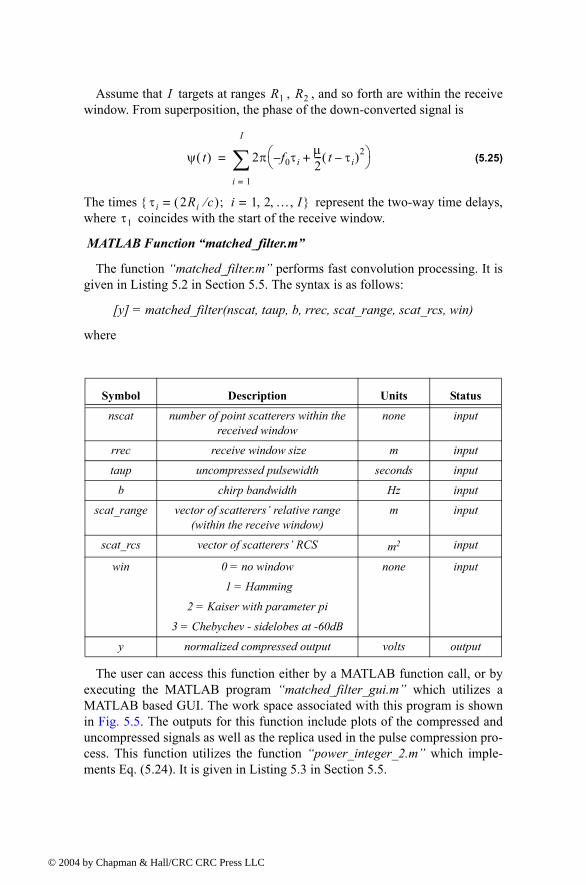
© 200
Assume that targets at ranges , , and so forth are within the receive window. From superposition, the phase of the down-converted signal is
(5.25)
The times represent the two-way time delays, where coincides with the start of the receive window.
MATLAB Function matched_filter.m
The function matched_filter.m performs fast convolution processing. It is given in Listing 5.2 in Section 5.5. The syntax is as follows:
[y] = matched_filter(nscat, taup, b, rrec, scat_range, scat_rcs, win)
where
The user can access this function either by a MATLAB function call, or by executing the MATLAB program matched_filter_gui.m which utilizes a MATLAB based GUI. The work space associated with this program is shown in Fig. 5.5. The outputs for this function include plots of the compressed and uncompressed signals as well as the replica used in the pulse compression pro-cess. This function utilizes the function power_integer_2.m which imple-ments Eq. (5.24). It is given in Listing 5.3 in Section 5.5.
Symbol Description Units Status
nscat number of point scatterers within the received window
none input
rrec receive window size m input
taup uncompressed pulsewidth seconds input
b chirp bandwidth Hz input
scat_range vector of scatterers relative range (within the receive window)
m input
scat_rcs vector of scatterers RCS m2 input
win 0 = no window
1 = Hamming
2 = Kaiser with parameter pi
3 = Chebychev - sidelobes at -60dB
none input
y normalized compressed output volts output
I R1 R2
ψ t( ) 2π f 0τiµ2--- t τi( )2+
i 1=
I
∑=
τi 2Ri c⁄( ) i; 1 2 … I, , ,= = τ1
4 by Chapman & Hall/CRC CRC Press LLC
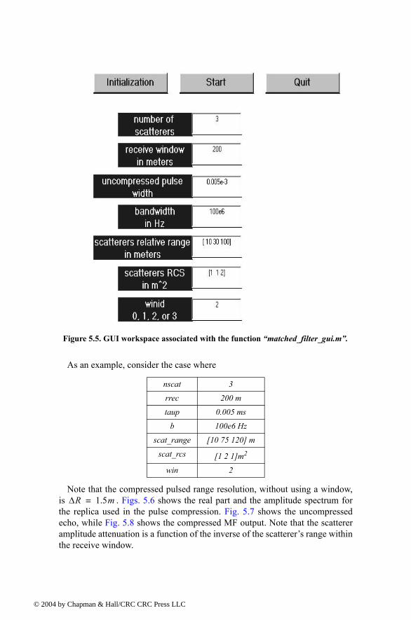
© 200
As an example, consider the case where
Note that the compressed pulsed range resolution, without using a window, is . Figs. 5.6 shows the real part and the amplitude spectrum for the replica used in the pulse compression. Fig. 5.7 shows the uncompressed echo, while Fig. 5.8 shows the compressed MF output. Note that the scatterer amplitude attenuation is a function of the inverse of the scatterers range within the receive window.
nscat 3
rrec 200 m
taup 0.005 ms
b 100e6 Hz
scat_range [10 75 120] m
scat_rcs [1 2 1]m2
win 2
Figure 5.5. GUI workspace associated with the function matched_filter_gui.m.
∆R 1.5m=
4 by Chapman & Hall/CRC CRC Press LLC
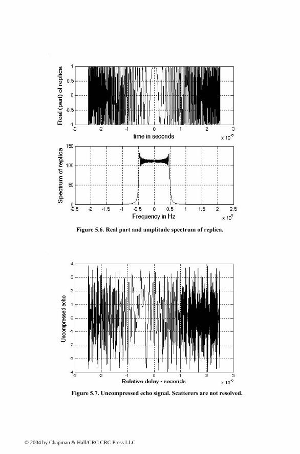
© 200
Figure 5.6. Real part and amplitude spectrum of replica.
Figure 5.7. Uncompressed echo signal. Scatterers are not resolved.
4 by Chapman & Hall/CRC CRC Press LLC
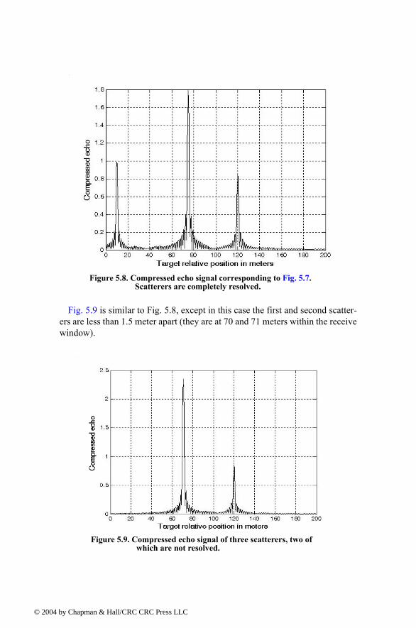
© 200
Fig. 5.9 is similar to Fig. 5.8, except in this case the first and second scatter-ers are less than 1.5 meter apart (they are at 70 and 71 meters within the receive window).
Figure 5.8. Compressed echo signal corresponding to Fig. 5.7. Scatterers are completely resolved.
Figure 5.9. Compressed echo signal of three scatterers, two of which are not resolved.
4 by Chapman & Hall/CRC CRC Press LLC
© 200
5.3.2. Stretch Processor
Stretch processing, also known as active correlation, is normally used to process extremely high bandwidth LFM waveforms. This processing technique consists of the following steps: First, the radar returns are mixed with a replica (reference signal) of the transmitted waveform. This is followed by Low Pass Filtering (LPF) and coherent detection. Next, Analog to Digital (A/D) conver-sion is performed; and finally, a bank of Narrow Band Filters (NBFs) is used in order to extract the tones that are proportional to target range, since stretch pro-cessing effectively converts time delay into frequency. All returns from the same range bin produce the same constant frequency. Fig. 5.10a shows a block diagram for a stretch processing receiver. The reference signal is an LFM waveform that has the same LFM slope as the transmitted LFM signal. It exists over the duration of the radar receive-window, which is computed from the difference between the radar maximum and minimum range. Denote the start frequency of the reference chirp as .
Consider the case when the radar receives returns from a few close (in time or range) targets, as illustrated in Fig. 5.10a. Mixing with the reference signal and performing low pass filtering are effectively equivalent to subtracting the return frequency chirp from the reference signal. Thus, the LPF output consists of constant tones corresponding to the targets positions. The normalized trans-mitted signal can be expressed by
(5.26)
where is the LFM coefficient and is the chirp start frequency. Assume a point scatterer at range . The signal received by the radar is
(5.27)
where is proportional to target RCS, antenna gain, and range attenuation. The time delay is
(5.28)
The reference signal is
(5.29)
The receive window in seconds is
(5.30)
fr
s1 t( ) 2π f0t µ2---t2+
cos= 0 t τ′≤ ≤
µ B τ′⁄= f0R
sr t( ) a 2π f0 t ∆τ( ) µ2--- t ∆τ( )2+
cos=
a∆τ
∆τ 2R c⁄=
sref t( ) 2 2π frtµ2---t2+
cos= 0 t Trec≤ ≤
Trec2 Rmax Rmin( )
c------------------------------------
2Rrec
c-------------= =
4 by Chapman & Hall/CRC CRC Press LLC
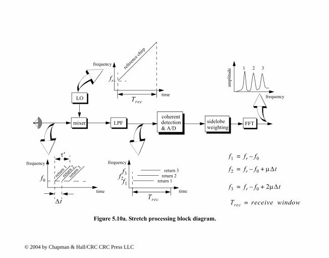
frequency
2 3
FFT
fr f0
fr f0 µ∆t+
fr f0 2µ∆t+
receive window=
return
1ret
urn 2
return
3
time
frequency
f0
time
frequency
fr
return 1return 2
return 3
time
frequency
f1
f3f2
refere
nce c
hirp
1
ampl
itude
τ′
mixer sidelobeLPFcoherentdetection& A/D weighting
LO
Figure 5.10a. Stretch processing block diagram.
∆t
Trec
Trec
f1 =
f2 =
f3 =
Trec
© 2004 by Chapman & Hall/CRC CRC Press LLC
© 200
It is customary to let . The output of the mixer is the product of the received and reference signals. After low pass filtering the signal is
(5.31)
Substituting Eq. (5.28) into (5.31) and collecting terms yield
(5.32)
and since , Eq. (5.32) is approximated by
(5.33)
The instantaneous frequency is
(5.34)
which clearly indicates that target range is proportional to the instantaneous frequency. Therefore, proper sampling of the LPF output and taking the FFT of the sampled sequence lead to the following conclusion: a peak at some fre-quency indicates presence of a target at range
(5.35)
Assume close targets at ranges , , and so forth ( ). From superposition, the total signal is
(5.36)
where are proportional to the targets cross sections, antenna gain, and range. The times represent the two-way time delays, where coincides with the start of the receive win-dow. Using Eq. (5.32) the overall signal at the output of the LPF can then be described by
(5.37)
And hence, target returns appear as constant frequency tones that can be resolved using the FFT. Consequently, determining the proper sampling rate and FFT size is very critical. The rest of this section presents a methodology for computing the proper FFT parameters required for stretch processing.
fr f0=
s0 t( ) a 2πf0∆τ 2πµ∆τt πµ ∆τ( )2+( )cos=
s0 t( ) a 4πBRcτ′
-------------- t 2R
c------- 2πf0
2πBRcτ′
-------------- +cos=
τ′ 2R c⁄»
s0 t( ) a 4πBRcτ′
-------------- t 4πR
c----------f0+cos≈
finst1
2π------
tdd 4πBR
cτ′--------------t 4πR
c----------f0+
2BRcτ′
-----------= =
f1
R1 f1cτ′ 2B⁄=
I R1 R2 R1 R2 … RI< < <
sr t( ) ai t( ) 2π f0 t τi( ) µ2--- t τi( )2+
cos
i 1=
I
∑=
ai t( ) i; 1 2 … I, , ,= τi 2Ri c⁄( ) i; 1 2 … I, , ,= =
τ1
so t( ) ai4πBRi
cτ′---------------- t
2Ri
c-------- 2πf0
2πBRi
cτ′----------------
+cos
i 1=
I
∑=
4 by Chapman & Hall/CRC CRC Press LLC
© 200
Assume a radar system using a stretch processor receiver. The pulsewidth is and the chirp bandwidth is . Since stretch processing is normally used in
extreme bandwidth cases (i.e., very large ), the receive window over which radar returns will be processed is typically limited to from a few meters to pos-sibly less than 100 meters. The compressed pulse range resolution is computed from Eq. (5.8). Declare the FFT size to be and its frequency resolution to be
. The frequency resolution can be computed using the following procedure: consider two adjacent point scatterers at range and . The minimum fre-quency separation, , between those scatterers so that they are resolved can be computed from Eq. (5.34). More precisely,
(5.38)
Substituting Eq. (5.8) into Eq. (5.38) yields
(5.39)
The maximum frequency resolvable by the FFT is limited to the region . Thus, the maximum resolvable frequency is
(5.40)
Using Eqs. (5.30) and (5.39) into Eq. (5.40) and collecting terms yield
(5.41)
For better implementation of the FFT, choose an FFT of size
(5.42)
is a nonzero positive integer. The sampling interval is then given by
(5.43)
MATLAB Function stretch.m
The function stretch.m presents a digital implementation of stretch pro-cessing. It is given in Listing 5.4 in Section 5.5. The syntax is as follows:
[y] = stretch (nscat, taup, f0, b, scat_range, rrec, scat_rcs, win)
where
τ′ BB
N∆f
R1 R2∆f
∆f f2 f12Bcτ′------- R2 R1( ) 2B
cτ′-------∆R= = =
∆f 2Bcτ′------- c
2B------- 1
τ′----= =
N∆f± 2⁄
N∆f2
----------2B Rmax Rmin( )
cτ′---------------------------------------->
2BRrec
cτ′-----------------=
N 2BTrec>
NFFT N≥ 2m=
m
∆f 1TsNFFT-----------------= Ts⇒ 1
∆fNFFT------------------=
4 by Chapman & Hall/CRC CRC Press LLC
© 200
The user can access this function either by a MATLAB function call or by exe-cuting the MATLAB program stretch_gui.m which utilizes MATLAB based GUI and is shown in Fig. 5.10b. The outputs of this function are the complex array and plots of the uncompressed and compressed echo signal versus time. As an example, consider the case where
Note that the compressed pulse range resolution, without using a window, is . Figs. 5.11 and 5.12, respectively, show the uncompressed and
compressed echo signals corresponding to this example. Fig. 5.13 is similar to Figs. 5.11 and 5.12 except in this case two of the scatterers are less than 15 cm apart (i.e., unresolved targets at ).
Symbol Description Units Status
nscat number of point scatterers within the received window
none input
taup uncompressed pulsewidth seconds input
f0 chirp start frequency Hz input
b chirp bandwidth Hz input
scat_range vector of scatterers range m input
rrec range receive window m input
scat_rcs vector of scatterers RCS m2 input
win 0 = no window
1 = Hamming
2 = Kaiser with parameter pi
3 = Chebychev - sidelobes at -60dB
none input
y compressed output volts output
nscat 3
taup 10 ms
f0 5.6 GHz
b 1 GHz
rrec 30 m
scat_range [2 5 10] m
scat_rcs [1, 1, 2] m2
win 2 (Kaiser)
y
∆R 0.15m=
Rrelative 3 3.1,[ ]m=
4 by Chapman & Hall/CRC CRC Press LLC
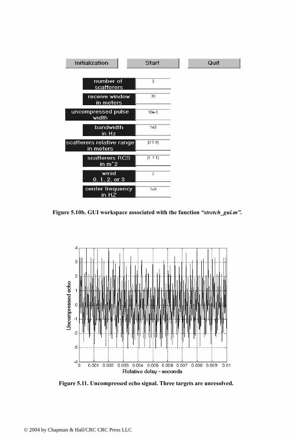
© 200
Figure 5.10b. GUI workspace associated with the function stretch_gui.m.
Figure 5.11. Uncompressed echo signal. Three targets are unresolved.
4 by Chapman & Hall/CRC CRC Press LLC
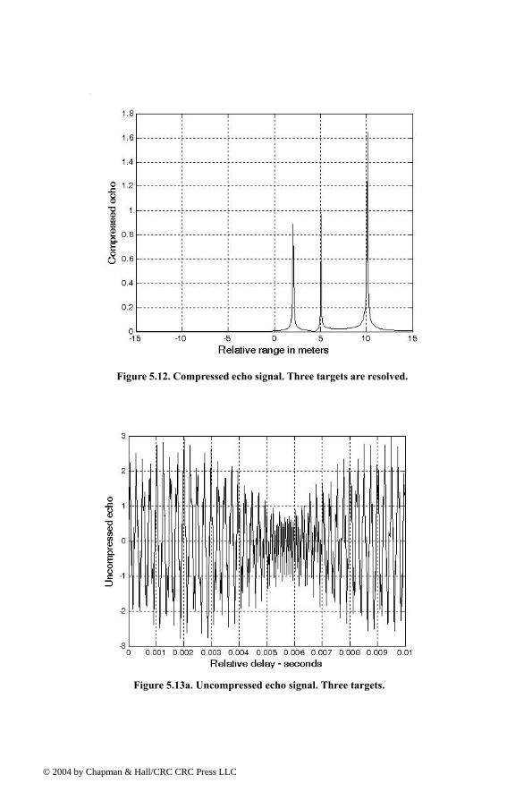
© 200
Figure 5.12. Compressed echo signal. Three targets are resolved.
Figure 5.13a. Uncompressed echo signal. Three targets.
4 by Chapman & Hall/CRC CRC Press LLC
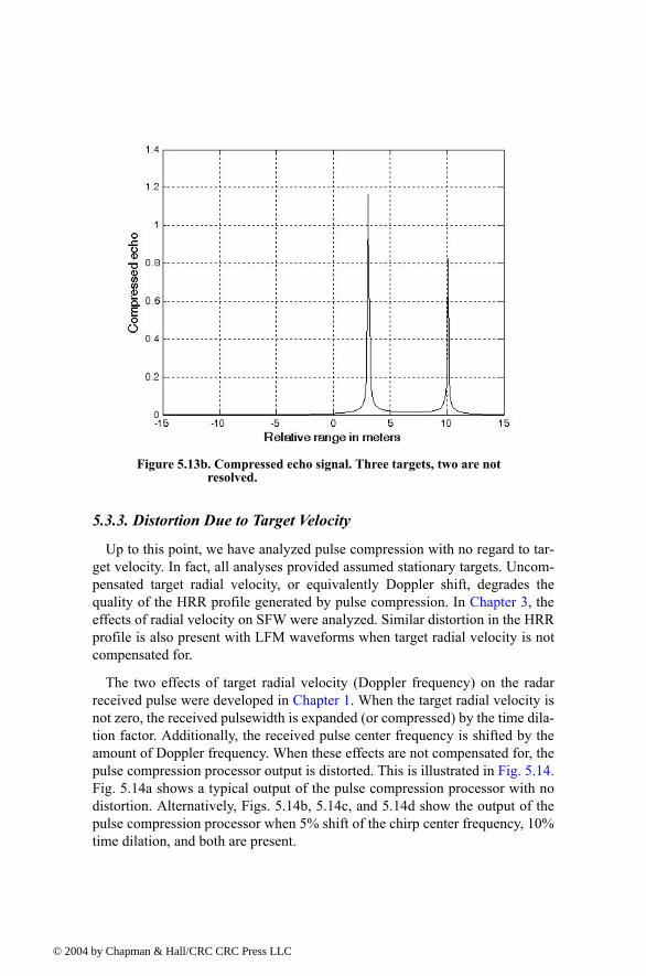
© 200
5.3.3. Distortion Due to Target Velocity
Up to this point, we have analyzed pulse compression with no regard to tar-get velocity. In fact, all analyses provided assumed stationary targets. Uncom-pensated target radial velocity, or equivalently Doppler shift, degrades the quality of the HRR profile generated by pulse compression. In Chapter 3, the effects of radial velocity on SFW were analyzed. Similar distortion in the HRR profile is also present with LFM waveforms when target radial velocity is not compensated for.
The two effects of target radial velocity (Doppler frequency) on the radar received pulse were developed in Chapter 1. When the target radial velocity is not zero, the received pulsewidth is expanded (or compressed) by the time dila-tion factor. Additionally, the received pulse center frequency is shifted by the amount of Doppler frequency. When these effects are not compensated for, the pulse compression processor output is distorted. This is illustrated in Fig. 5.14. Fig. 5.14a shows a typical output of the pulse compression processor with no distortion. Alternatively, Figs. 5.14b, 5.14c, and 5.14d show the output of the pulse compression processor when 5% shift of the chirp center frequency, 10% time dilation, and both are present.
Figure 5.13b. Compressed echo signal. Three targets, two are not resolved.
4 by Chapman & Hall/CRC CRC Press LLC
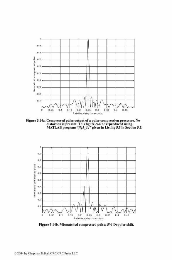
© 200
Figure 5.14a. Compressed pulse output of a pulse compression processor. No distortion is present. This figure can be reproduced using MATLAB program fig5_14 given in Listing 5.5 in Section 5.5.
0 0.05 0.1 0.15 0.2 0.25 0.3 0.35 0.4 0.45
0.1
0.2
0.3
0.4
0.5
0.6
0.7
0.8
0.9
1
R ela t ive de lay - s ec onds
No
rma
lize
d c
om
pre
ss
ed
pu
lse
Figure 5.14b. Mismatched compressed pulse; 5% Doppler shift.
0 0 .0 5 0 .1 0 .1 5 0 .2 0 .2 5 0 .3 0 .3 5 0 .4 0 .4 5
0 .1
0 .2
0 .3
0 .4
0 .5
0 .6
0 .7
0 .8
0 .9
1
R e la t ive d e la y - s e c o n d s
No
rma
lize
d c
om
pre
ss
ed
pu
lse
4 by Chapman & Hall/CRC CRC Press LLC
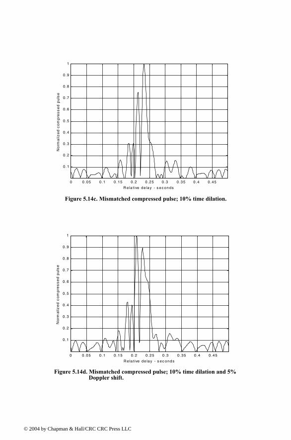
© 200
Figure 5.14c. Mismatched compressed pulse; 10% time dilation.
0 0 .05 0 .1 0 .15 0 .2 0 .25 0 .3 0.35 0.4 0 .45
0.1
0.2
0 .3
0 .4
0 .5
0 .6
0 .7
0 .8
0 .9
1
R ela t ive de lay - s ec onds
No
rma
lize
d c
om
pre
ss
ed
pu
lse
Figure 5.14d. Mismatched compressed pulse; 10% time dilation and 5% Doppler shift.
0 0 .05 0.1 0 .15 0.2 0 .25 0 .3 0 .35 0 .4 0 .45
0.1
0 .2
0 .3
0 .4
0 .5
0 .6
0 .7
0 .8
0 .9
1
R e la t ive de lay - s ec onds
No
rma
lize
d c
om
pre
ss
ed
pu
lse
4 by Chapman & Hall/CRC CRC Press LLC
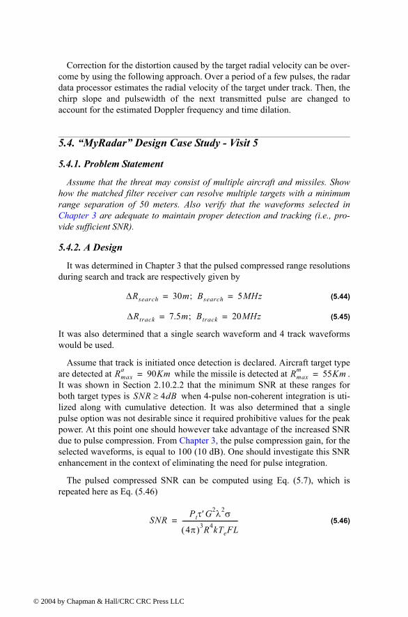
© 200
Correction for the distortion caused by the target radial velocity can be over-come by using the following approach. Over a period of a few pulses, the radar data processor estimates the radial velocity of the target under track. Then, the chirp slope and pulsewidth of the next transmitted pulse are changed to account for the estimated Doppler frequency and time dilation.
5.4. MyRadar Design Case Study - Visit 5
5.4.1. Problem Statement
Assume that the threat may consist of multiple aircraft and missiles. Show how the matched filter receiver can resolve multiple targets with a minimum range separation of 50 meters. Also verify that the waveforms selected in Chapter 3 are adequate to maintain proper detection and tracking (i.e., pro-vide sufficient SNR).
5.4.2. A Design
It was determined in Chapter 3 that the pulsed compressed range resolutions during search and track are respectively given by
(5.44)
(5.45)
It was also determined that a single search waveform and 4 track waveforms would be used.
Assume that track is initiated once detection is declared. Aircraft target type are detected at while the missile is detected at . It was shown in Section 2.10.2.2 that the minimum SNR at these ranges for both target types is when 4-pulse non-coherent integration is uti-lized along with cumulative detection. It was also determined that a single pulse option was not desirable since it required prohibitive values for the peak power. At this point one should however take advantage of the increased SNR due to pulse compression. From Chapter 3, the pulse compression gain, for the selected waveforms, is equal to 100 (10 dB). One should investigate this SNR enhancement in the context of eliminating the need for pulse integration.
The pulsed compressed SNR can be computed using Eq. (5.7), which is repeated here as Eq. (5.46)
(5.46)
∆Rsearch 30m Bsearch; 5MHz= =
∆Rtrack 7.5m Btrack; 20MHz= =
Rmaxa 90Km= Rmax
m 55Km=
SNR 4dB≥
SNRPtτ′G
2λ2σ
4π( )3R4kTeFL------------------------------------=
4 by Chapman & Hall/CRC CRC Press LLC
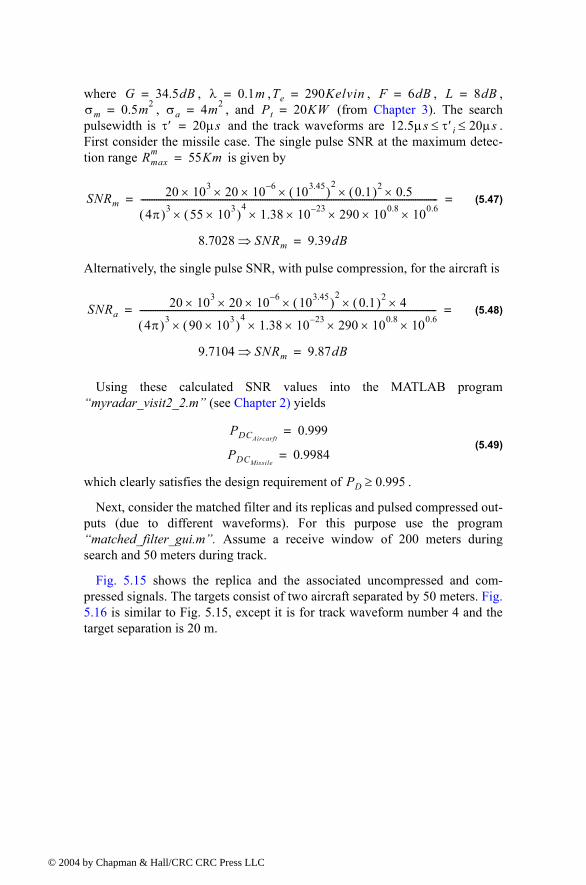
© 200
where , , , , , , , and (from Chapter 3). The search
pulsewidth is and the track waveforms are . First consider the missile case. The single pulse SNR at the maximum detec-tion range is given by
(5.47)
Alternatively, the single pulse SNR, with pulse compression, for the aircraft is
(5.48)
Using these calculated SNR values into the MATLAB program myradar_visit2_2.m (see Chapter 2) yields
(5.49)
which clearly satisfies the design requirement of .
Next, consider the matched filter and its replicas and pulsed compressed out-puts (due to different waveforms). For this purpose use the program matched_filter_gui.m. Assume a receive window of 200 meters during search and 50 meters during track.
Fig. 5.15 shows the replica and the associated uncompressed and com-pressed signals. The targets consist of two aircraft separated by 50 meters. Fig. 5.16 is similar to Fig. 5.15, except it is for track waveform number 4 and the target separation is 20 m.
G 34.5dB= λ 0.1m= Te 290Kelvin= F 6dB= L 8dB=σm 0.5m2= σa 4m2= Pt 20KW=
τ′ 20µs= 12.5µs τ≤ ′i 20µs≤
Rmaxm 55Km=
SNRm20 103 20 10 6 103.45( )
20.1( )2× 0.5×××××
4π( )3 55 103×( )4
1.38× 10 23× 290 100.8× 100.6×××--------------------------------------------------------------------------------------------------------------------------------------
8.7028 SNRm⇒ 9.39dB
= =
=
SNRa20 103 20 10 6 103.45( )
20.1( )2× 4×××××
4π( )3 90 103×( )4
1.38× 10 23× 290 100.8× 100.6×××--------------------------------------------------------------------------------------------------------------------------------------
9.7104 SNRm⇒ 9.87dB
= =
=
PDCAircarft0.999=
PDCMissile0.9984=
PD 0.995≥
4 by Chapman & Hall/CRC CRC Press LLC
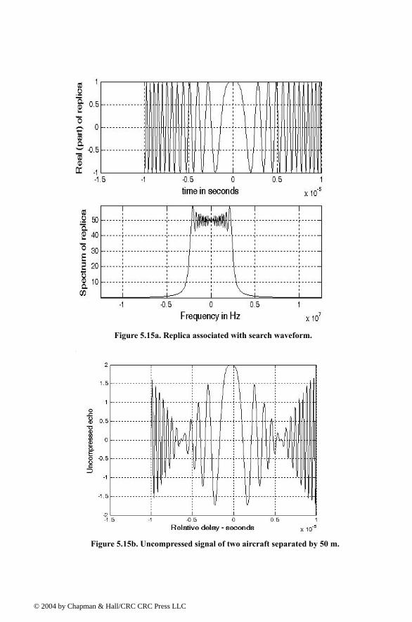
© 200
Figure 5.15a. Replica associated with search waveform.
Figure 5.15b. Uncompressed signal of two aircraft separated by 50 m.
4 by Chapman & Hall/CRC CRC Press LLC
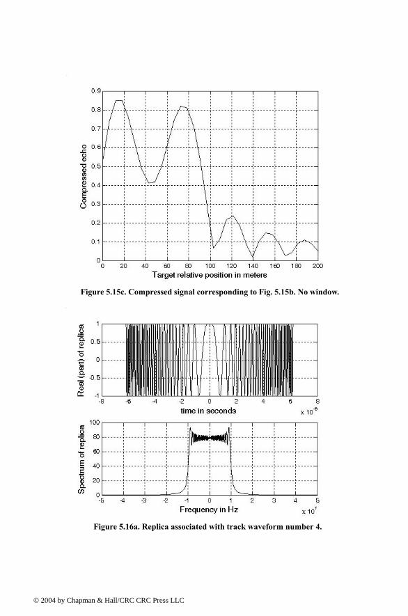
© 200
Figure 5.15c. Compressed signal corresponding to Fig. 5.15b. No window.
Figure 5.16a. Replica associated with track waveform number 4.
4 by Chapman & Hall/CRC CRC Press LLC
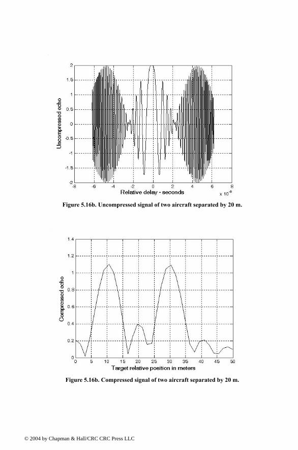
© 200
Figure 5.16b. Uncompressed signal of two aircraft separated by 20 m.
Figure 5.16b. Compressed signal of two aircraft separated by 20 m.
4 by Chapman & Hall/CRC CRC Press LLC

© 200
5.5. MATLAB Program and Function ListingsThis section presents listings for all MATLAB programs/functions used in
this chapter. The user is strongly advised to rerun the MATLAB programs in order to enhance his understanding of this chapters material.
Listing 5.1. MATLAB Program fig5_3.m% use this program to reproduce Fig. 5.3 of textclear allclose allnscat = 2; %two point scattererstaup = 10e-6; % 10 microsecond uncompressed pulseb = 50.0e6; % 50 MHz bandwidthrrec = 50 ; % 50 meter processing windowscat_range = [15 25] ; % scatterers are 15 and 25 meters into windowscat_rcs = [1 2]; % RCS 1 m^2 and 2m^2winid = 0; %no window used[y] = matched_filter(nscat,taup,b,rrec,scat_range,scat_rcs,winid);
Listing 5.2. MATLAB Function matched_filter.mfunction [y] = matched_filter(nscat,taup,b,rrec,scat_range,scat_rcs,winid)eps = 1.0e-16;% time bandwidth producttime_B_product = b * taup;if(time_B_product < 5 ) fprintf('********** Time Bandwidth product is TOO SMALL *********') fprintf('\n Change b and or taup') returnend% speed of lightc = 3.e8; % number of samplesn = fix(5 * taup * b)% initialize input, output and replica vectorsx(nscat,1:n) = 0.;y(1:n) = 0.;replica(1:n) = 0.;% determine proper windowif( winid == 0.) win(1:n) = 1.; win =win';else if(winid == 1.)
4 by Chapman & Hall/CRC CRC Press LLC
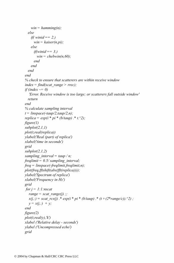
© 200
win = hamming(n); else if( winid == 2.) win = kaiser(n,pi); else if(winid == 3.) win = chebwin(n,60); end end endend% check to ensure that scatterers are within receive windowindex = find(scat_range > rrec);if (index ~= 0) 'Error. Receive window is too large; or scatterers fall outside window' returnend% calculate sampling intervalt = linspace(-taup/2,taup/2,n);replica = exp(i * pi * (b/taup) .* t.^2);figure(1)subplot(2,1,1)plot(t,real(replica))ylabel('Real (part) of replica')xlabel('time in seconds')gridsubplot(2,1,2)sampling_interval = taup / n;freqlimit = 0.5/ sampling_interval;freq = linspace(-freqlimit,freqlimit,n);plot(freq,fftshift(abs(fft(replica))));ylabel('Spectrum of replica')xlabel('Frequency in Hz')grid for j = 1:1:nscat range = scat_range(j) ;; x(j,:) = scat_rcs(j) .* exp(i * pi * (b/taup) .* (t +(2*range/c)).^2) ; y = x(j,:) + y;endfigure(2)plot(t,real(y),'k')xlabel ('Relative delay - seconds')ylabel ('Uncompressed echo')grid
4 by Chapman & Hall/CRC CRC Press LLC
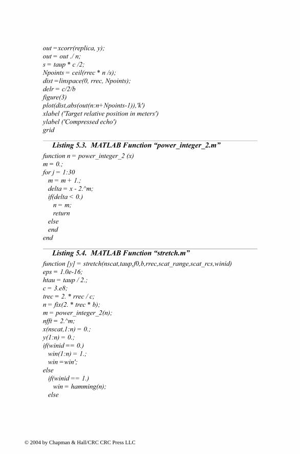
© 200
out =xcorr(replica, y);out = out ./ n;s = taup * c /2;Npoints = ceil(rrec * n /s);dist =linspace(0, rrec, Npoints);delr = c/2/bfigure(3)plot(dist,abs(out(n:n+Npoints-1)),'k')xlabel ('Target relative position in meters')ylabel ('Compressed echo')grid
Listing 5.3. MATLAB Function power_integer_2.mfunction n = power_integer_2 (x)m = 0.;for j = 1:30 m = m + 1.; delta = x - 2.^m; if(delta < 0.) n = m; return else endend
Listing 5.4. MATLAB Function stretch.mfunction [y] = stretch(nscat,taup,f0,b,rrec,scat_range,scat_rcs,winid)eps = 1.0e-16;htau = taup / 2.;c = 3.e8;trec = 2. * rrec / c;n = fix(2. * trec * b);m = power_integer_2(n);nfft = 2.^m;x(nscat,1:n) = 0.;y(1:n) = 0.;if(winid == 0.) win(1:n) = 1.; win =win';else if(winid == 1.) win = hamming(n); else
4 by Chapman & Hall/CRC CRC Press LLC
© 200
if( winid == 2.) win = kaiser(n,pi); else if(winid == 3.) win = chebwin(n,60); end end endenddeltar = c / 2. / b;max_rrec = deltar * nfft / 2.;maxr = max(scat_range);if(rrec > max_rrec | maxr >= rrec ) 'Error. Receive window is too large; or scatterers fall outside window' returnendt = linspace(0,taup,n);for j = 1:1:nscat range = scat_range(j);% + rmin; psi1 = 4. * pi * range * f0 / c - ... 4. * pi * b * range * range / c / c/ taup; psi2 = (2*4. * pi * b * range / c / taup) .* t; x(j,:) = scat_rcs(j) .* exp(i * psi1 + i .* psi2); y = y + x(j,:);endfigure(1)plot(t,real(y),'k')xlabel ('Relative delay - seconds')ylabel ('Uncompressed echo')ywin = y .* win';yfft = fft(y,n) ./ n;out= fftshift(abs(yfft));figure(2)delinc = rrec/ n;%dist = linspace(-delinc-rrec/2,rrec/2,n);dist = linspace((-rrec/2), rrec/2,n);plot(dist,out,'k')xlabel ('Relative range in meters')ylabel ('Compressed echo')axis autogrid
4 by Chapman & Hall/CRC CRC Press LLC
© 200
Listing 5.5. MATLAB Program fig5_14.m% use this program to reproduce Fig. 5.14 of textclear alleps = 1.5e-5;t = 0:0.001:.5; y = chirp(t,0,.25,20);figure(1)plot(t,y);yfft = fft(y,512) ;ycomp = fftshift(abs(ifft(yfft .* conj(yfft))));maxval = max (ycomp);ycomp = eps + ycomp ./ maxval; figure(1)del = .5 /512.;tt = 0:del:.5-eps;plot (tt,ycomp,'k')axis tightxlabel ('Relative delay - seconds');ylabel('Normalized compressed pulse')gridy1 = chirp (t,0,.25,21); % change center frequencyy1fft = fft(y1,512);y1comp = fftshift(abs(ifft(y1fft .* conj(yfft))));maxval = max (y1comp);y1comp = eps + y1comp ./ maxval; figure(2)plot (tt,y1comp,'k')axis tightxlabel ('Relative delay - seconds');ylabel('Normalized compressed pulse')gridt = 0:0.001:.45; % change pulsewidth y2 = chirp (t,0,.225,20);y2fft = fft(y2,512);y2comp = fftshift(abs(ifft(y2fft .* conj(yfft))));maxval = max (y2comp);y2comp = eps + y2comp ./ maxval; figure(3)plot (tt,y2comp,'k')axis tightxlabel ('Relative delay - seconds');ylabel('Normalized compressed pulse')grid
4 by Chapman & Hall/CRC CRC Press LLC
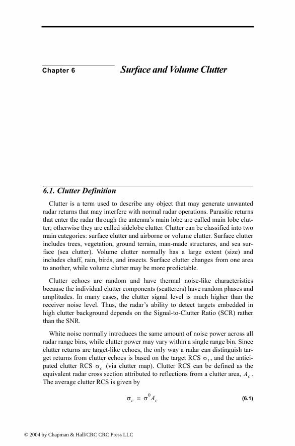
© 200
Chapter 6 Surface and Volume Clutter
6.1. Clutter DefinitionClutter is a term used to describe any object that may generate unwanted
radar returns that may interfere with normal radar operations. Parasitic returns that enter the radar through the antennas main lobe are called main lobe clut-ter; otherwise they are called sidelobe clutter. Clutter can be classified into two main categories: surface clutter and airborne or volume clutter. Surface clutter includes trees, vegetation, ground terrain, man-made structures, and sea sur-face (sea clutter). Volume clutter normally has a large extent (size) and includes chaff, rain, birds, and insects. Surface clutter changes from one area to another, while volume clutter may be more predictable.
Clutter echoes are random and have thermal noise-like characteristics because the individual clutter components (scatterers) have random phases and amplitudes. In many cases, the clutter signal level is much higher than the receiver noise level. Thus, the radars ability to detect targets embedded in high clutter background depends on the Signal-to-Clutter Ratio (SCR) rather than the SNR.
White noise normally introduces the same amount of noise power across all radar range bins, while clutter power may vary within a single range bin. Since clutter returns are target-like echoes, the only way a radar can distinguish tar-get returns from clutter echoes is based on the target RCS , and the antici-pated clutter RCS (via clutter map). Clutter RCS can be defined as the equivalent radar cross section attributed to reflections from a clutter area, . The average clutter RCS is given by
(6.1)
σtσc
Ac
σc σ0Ac=
4 by Chapman & Hall/CRC CRC Press LLC
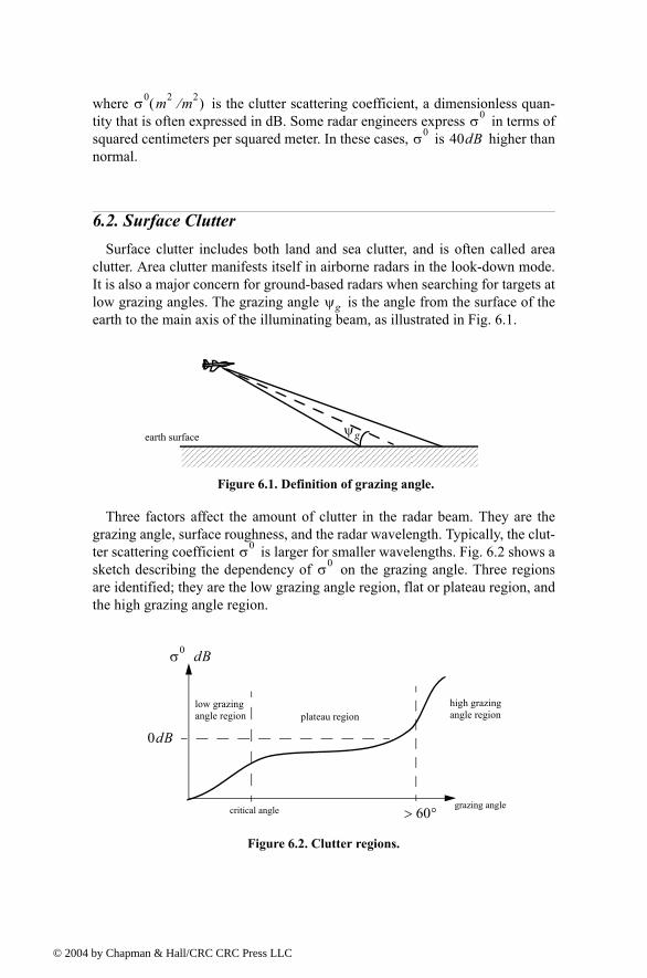
© 200
where is the clutter scattering coefficient, a dimensionless quan-tity that is often expressed in dB. Some radar engineers express in terms of squared centimeters per squared meter. In these cases, is higher than normal.
6.2. Surface ClutterSurface clutter includes both land and sea clutter, and is often called area
clutter. Area clutter manifests itself in airborne radars in the look-down mode. It is also a major concern for ground-based radars when searching for targets at low grazing angles. The grazing angle is the angle from the surface of the earth to the main axis of the illuminating beam, as illustrated in Fig. 6.1.
Three factors affect the amount of clutter in the radar beam. They are the grazing angle, surface roughness, and the radar wavelength. Typically, the clut-ter scattering coefficient is larger for smaller wavelengths. Fig. 6.2 shows a sketch describing the dependency of on the grazing angle. Three regions are identified; they are the low grazing angle region, flat or plateau region, and the high grazing angle region.
σ0 m2 m2⁄( )σ0
σ0 40dB
ψg
ψgearth surface
Figure 6.1. Definition of grazing angle.
σ0
σ0
σ0 dB
grazing angle
0dB
critical angle 60°>
Figure 6.2. Clutter regions.
high grazingangle regionplateau region
low grazingangle region
4 by Chapman & Hall/CRC CRC Press LLC
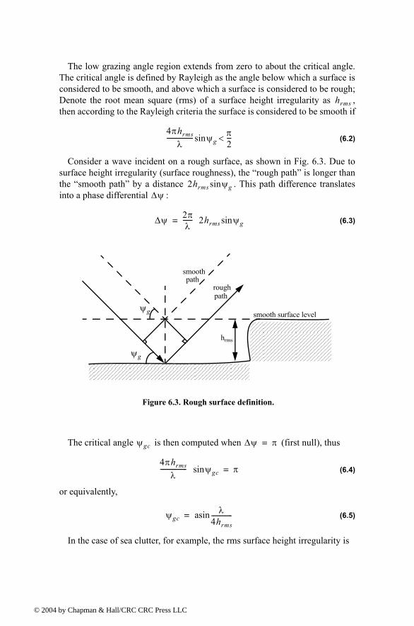
© 200
The low grazing angle region extends from zero to about the critical angle. The critical angle is defined by Rayleigh as the angle below which a surface is considered to be smooth, and above which a surface is considered to be rough; Denote the root mean square (rms) of a surface height irregularity as , then according to the Rayleigh criteria the surface is considered to be smooth if
(6.2)
Consider a wave incident on a rough surface, as shown in Fig. 6.3. Due to surface height irregularity (surface roughness), the rough path is longer than the smooth path by a distance . This path difference translates into a phase differential :
(6.3)
The critical angle is then computed when (first null), thus
(6.4)
or equivalently,
(6.5)
In the case of sea clutter, for example, the rms surface height irregularity is
hrms
4πhrms
λ----------------- ψgsin π
2---<
2hrms ψgsin∆ψ
∆ψ 2πλ
------ 2hrms ψgsin=
ψg
ψg
smoothpath
roughpath
smooth surface level
hrms
Figure 6.3. Rough surface definition.
ψgc ∆ψ π=
4πhrms
λ----------------- ψgcsin π=
ψgcλ
4hrms-------------asin=
4 by Chapman & Hall/CRC CRC Press LLC
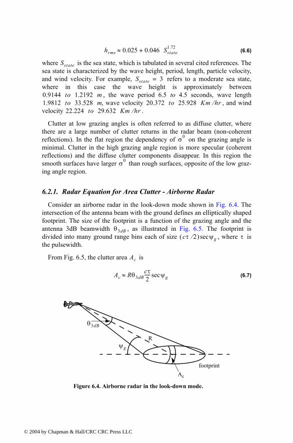
© 200
(6.6)
where is the sea state, which is tabulated in several cited references. The sea state is characterized by the wave height, period, length, particle velocity, and wind velocity. For example, refers to a moderate sea state, where in this case the wave height is approximately between
, the wave period 6.5 to 4.5 seconds, wave length , wave velocity , and wind
velocity .
Clutter at low grazing angles is often referred to as diffuse clutter, where there are a large number of clutter returns in the radar beam (non-coherent reflections). In the flat region the dependency of on the grazing angle is minimal. Clutter in the high grazing angle region is more specular (coherent reflections) and the diffuse clutter components disappear. In this region the smooth surfaces have larger than rough surfaces, opposite of the low graz-ing angle region.
6.2.1. Radar Equation for Area Clutter - Airborne Radar
Consider an airborne radar in the look-down mode shown in Fig. 6.4. The intersection of the antenna beam with the ground defines an elliptically shaped footprint. The size of the footprint is a function of the grazing angle and the antenna 3dB beamwidth , as illustrated in Fig. 6.5. The footprint is divided into many ground range bins each of size , where is the pulsewidth.
From Fig. 6.5, the clutter area is
(6.7)
hrms 0.025 0.046 Sstate1.72+≈
Sstate
Sstate 3=
0.9144 to 1.2192 m1.9812 to 33.528 m 20.372 to 25.928 Km hr⁄
22.224 to 29.632 Km hr⁄
σ0
σ0
θ3dBcτ 2⁄( ) ψgsec τ
Ac
Ac Rθ3dBcτ2----- ψgsec≈
ψg
Figure 6.4. Airborne radar in the look-down mode.
Ac
footprint
R
θ3dB
4 by Chapman & Hall/CRC CRC Press LLC
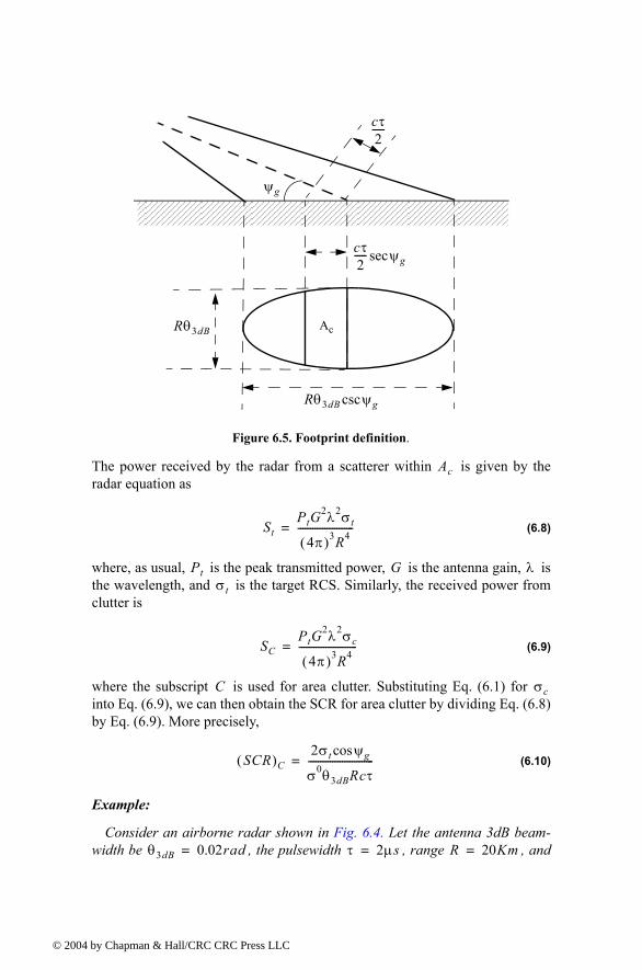
© 200
The power received by the radar from a scatterer within is given by the radar equation as
(6.8)
where, as usual, is the peak transmitted power, is the antenna gain, is the wavelength, and is the target RCS. Similarly, the received power from clutter is
(6.9)
where the subscript is used for area clutter. Substituting Eq. (6.1) for into Eq. (6.9), we can then obtain the SCR for area clutter by dividing Eq. (6.8) by Eq. (6.9). More precisely,
(6.10)
Example:
Consider an airborne radar shown in Fig. 6.4. Let the antenna 3dB beam-width be , the pulsewidth , range , and
cτ2-----
AcRθ3dB
Rθ3dB ψgcsc
cτ2----- ψgsec
ψg
Figure 6.5. Footprint definition.
Ac
StPtG
2λ2σt
4π( )3R4-----------------------=
Pt G λσt
SCPtG
2λ2σc
4π( )3R4------------------------=
C σc
SCR( )C2σt ψgcos
σ0θ3dBRcτ---------------------------=
θ3dB 0.02rad= τ 2µs= R 20Km=
4 by Chapman & Hall/CRC CRC Press LLC
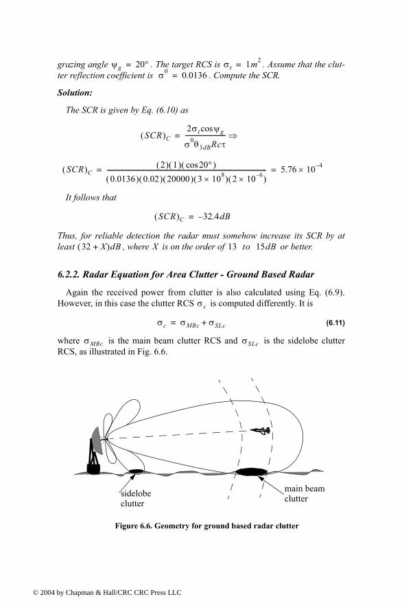
© 200
grazing angle . The target RCS is . Assume that the clut-ter reflection coefficient is . Compute the SCR.
Solution:
The SCR is given by Eq. (6.10) as
It follows that
Thus, for reliable detection the radar must somehow increase its SCR by at least , where is on the order of or better.
6.2.2. Radar Equation for Area Clutter - Ground Based Radar
Again the received power from clutter is also calculated using Eq. (6.9). However, in this case the clutter RCS is computed differently. It is
(6.11)
where is the main beam clutter RCS and is the sidelobe clutter RCS, as illustrated in Fig. 6.6.
ψg 20°= σt 1m2=σ0 0.0136=
SCR( )C2σt ψgcos
σ0θ3dBRcτ--------------------------- ⇒=
SCR( )C2( ) 1( ) 20°cos( )
0.0136( ) 0.02( ) 20000( ) 3 108×( ) 2 10 6×( )--------------------------------------------------------------------------------------------------------- 5.76 10 4×= =
SCR( )C 32.4dB=
32 X+( )dB X 13 to 15dB
σc
σc σMBc σSLc+=
σMBc σSLc
Figure 6.6. Geometry for ground based radar clutter
main beam cluttersidelobe
clutter
4 by Chapman & Hall/CRC CRC Press LLC
© 200
In order to calculate the total clutter RCS given in Eq. (6.11), one must first compute the corresponding clutter areas for both the main beam and the side-lobes. For this purpose, consider the geometry shown in Fig. 6.7. The angles
represent the antenna 3-dB azimuth and elevation beamwidths, respectively. The radar height (from the ground to the phase center of the antenna) is denoted by , while the target height is denoted by . The radar slant range is , and its ground projection is . The range resolution is and its ground projection is . The main beam clutter area is denoted by
and the sidelobe clutter area is denoted by .
θA and θE
hr htR Rg ∆R
∆RgAMBc ASLc
earth surfacehr
ht
R
Rg
θE
θe
θr
∆Rg
∆Rg
θA
sidelobeclutter region
sidelobeclutter region
main beamclutter region
Figure 6.7. Clutter geometry for ground based radar. Side view and top view.
R
antenna boresight
4 by Chapman & Hall/CRC CRC Press LLC
© 200
From Fig. 6.7 the following relations can be derived
(6.12)
(6.13)
(6.14)
where is the radar range resolution. The slant range ground projection is
(6.15)
It follows that the main beam and the sidelobe clutter areas are
(6.16)
(6.17)
Assume a radar antenna beam of the form
(6.18)
(6.19)
Then the main beam clutter RCS is
(6.20)
and the sidelobe clutter RCS is
(6.21)
where the quantity is the root-mean-square (rms) for the antenna side-lobe level.
Finally, in order to account for the variation of the clutter RCS versus range, one can calculate the total clutter RCS as a function of range. It is given by
(6.22)
where is the radar range to the horizon calculated as
θr hr R⁄( )asin=
θe ht hr( ) R⁄( )asin=
∆Rg ∆R θrcos=
∆R
Rg R θrcos=
AMBc ∆Rg Rg θA=
ASLc ∆Rg πRg=
G θ( )
G θ( ) 2.776θ2
θE2
-------------------
exp= Gaussian⇒
G θ( )
2.78 θθE-----
sin
2.78 θθE-----
------------------------------
2
0
θπθE
2.78----------≤;
elsewhere;
=x( )sin
x---------------
2⇒
σMBc σ0AMBcG2 θe θr+( ) σ0∆Rg Rg θAG2 θe θr+( )= =
σSLc σ0ASLc SLrms( )2 σ0∆Rg πRg SLrms( )2= =
SLrms
σc R( )σMBc σSLc+
1 R Rh⁄( )4+( )-----------------------------------=
Rh
4 by Chapman & Hall/CRC CRC Press LLC
© 200
(6.23)
where is the Earths radius equal to . The denominator in Eq. (6.22) is put in that format in order to account for refraction and for round (spherical) Earth effects.
The radar SNR due to a target at range is
(6.24)
where, as usual, is the peak transmitted power, is the antenna gain, is the wavelength, is the target RCS, is Boltzmans constant, is the effective noise temperature, is the radar operating bandwidth, is the receiver noise figure, and is the total radar losses. Similarly, the Clutter-to-Noise (CNR) at the radar is
(6.25)
where the is calculated using Eq. (6.21).
When the clutter statistic is Gaussian, the clutter signal return and the noise return can be combined, and a new value for determining the radar measure-ment accuracy is derived from the Signal-to-Clutter+Noise-Ratio, denoted by SIR. It is given by
(6.26)
Note that the is computed by dividing Eq.(6.24) by Eq. (6.25).
MATLAB Function clutter_rcs.m
The function clutter_rcs.m implements Eq. (6.22); it is given in Listing 6.1 in Section 6.6. It also generates plots of the clutter RCS and the CNR ver-sus the radar slant range. Its outputs include the clutter RCS in dBsm and the CNR in dB. The syntax is as follows:
[sigmaC,CNR] = clutter_rcs(sigma0, thetaE, thetaA, SL, range, hr, ht, pt, f0, b, t0, f, l, ant_id)
where
Rh8hrre
3-------------=
re 6371Km
R
SNRPtG
2λ2σt
4π( )3R4kToBFL----------------------------------------=
Pt G λσt k T0
B FL
CNRPtG
2λ2σc
4π( )3R4kToBFL----------------------------------------=
σc
SIR 11
SNR----------- 1
SCR-----------+
-----------------------------=
SCR
4 by Chapman & Hall/CRC CRC Press LLC
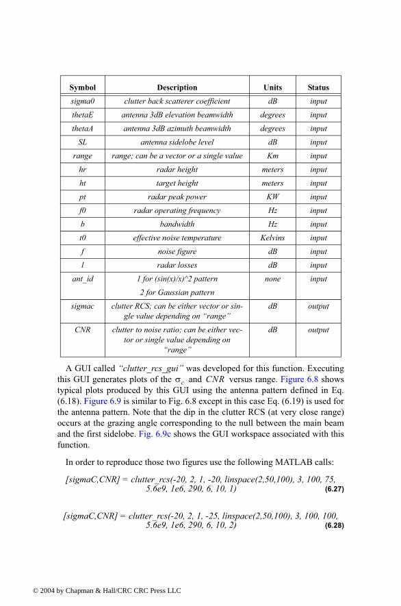
© 200
A GUI called clutter_rcs_gui was developed for this function. Executing this GUI generates plots of the and versus range. Figure 6.8 shows typical plots produced by this GUI using the antenna pattern defined in Eq. (6.18). Figure 6.9 is similar to Fig. 6.8 except in this case Eq. (6.19) is used for the antenna pattern. Note that the dip in the clutter RCS (at very close range) occurs at the grazing angle corresponding to the null between the main beam and the first sidelobe. Fig. 6.9c shows the GUI workspace associated with this function.
In order to reproduce those two figures use the following MATLAB calls:
[sigmaC,CNR] = clutter_rcs(-20, 2, 1, -20, linspace(2,50,100), 3, 100, 75, 5.6e9, 1e6, 290, 6, 10, 1) (6.27)
[sigmaC,CNR] = clutter_rcs(-20, 2, 1, -25, linspace(2,50,100), 3, 100, 100, 5.6e9, 1e6, 290, 6, 10, 2) (6.28)
Symbol Description Units Status
sigma0 clutter back scatterer coefficient dB input
thetaE antenna 3dB elevation beamwidth degrees input
thetaA antenna 3dB azimuth beamwidth degrees input
SL antenna sidelobe level dB input
range range; can be a vector or a single value Km input
hr radar height meters input
ht target height meters input
pt radar peak power KW input
f0 radar operating frequency Hz input
b bandwidth Hz input
t0 effective noise temperature Kelvins input
f noise figure dB input
l radar losses dB input
ant_id 1 for (sin(x)/x)^2 pattern
2 for Gaussian pattern
none input
sigmac clutter RCS; can be either vector or sin-gle value depending on range
dB output
CNR clutter to noise ratio; can be either vec-tor or single value depending on
range
dB output
σc CNR
4 by Chapman & Hall/CRC CRC Press LLC
© 200
Figure 6.8a. Clutter RCS versus range using the function call in Eq. (6.27).
Figure 6.8b. CNR versus range using the function call in Eq. (6.27).
4 by Chapman & Hall/CRC CRC Press LLC
© 200
Figure 6.9a. Clutter RCS versus range using the function call in Eq. (6.28).
Figure 6.9b. CNR versus range using the function call in Eq. (6.28).
4 by Chapman & Hall/CRC CRC Press LLC
© 200
Figure 6.9c. GUI workspace for clutter_rcs_gui.m.
4 by Chapman & Hall/CRC CRC Press LLC
© 200
6.3. Volume ClutterVolume clutter has large extents and includes rain (weather), chaff, birds,
and insects. The volume clutter coefficient is normally expressed in square meters (RCS per resolution volume). Birds, insects, and other flying particles are often referred to as angle clutter or biological clutter.
As mentioned earlier, chaff is used as an ECM technique by hostile forces. It consists of a large number of dipole reflectors with large RCS values. Histori-cally, chaff was made of aluminum foil; however, in recent years most chaff is made of the more rigid fiberglass with conductive coating. The maximum chaff RCS occurs when the dipole length is one half the radar wavelength.
Weather or rain clutter is easier to suppress than chaff, since rain droplets can be viewed as perfect small spheres. We can use the Rayleigh approxima-tion of a perfect sphere to estimate the rain droplets RCS. The Rayleigh approximation, without regard to the propagation medium index of refraction is:
(6.29)
where , and is radius of a rain droplet.
Electromagnetic waves when reflected from a perfect sphere become strongly co-polarized (have the same polarization as the incident waves). Con-sequently, if the radar transmits, for example, a right-hand-circular (RHC) polarized wave, then the received waves are left-hand-circular (LHC) polar-ized, because they are propagating in the opposite direction. Therefore, the back-scattered energy from rain droplets retains the same wave rotation (polar-ization) as the incident wave, but has a reversed direction of propagation. It follows that radars can suppress rain clutter by co-polarizing the radar transmit and receive antennas.
Denote as RCS per unit resolution volume . It is computed as the sum of all individual scatterers RCS within the volume,
(6.30)
where is the total number of scatterers within the resolution volume. Thus, the total RCS of a single resolution volume is
(6.31)
L
σ 9πr2 kr( )4= r λ«
k 2π λ⁄= r
η VW
η σi
i 1=
N
∑=
N
σW σiVW
i 1=
N
∑=
4 by Chapman & Hall/CRC CRC Press LLC
© 200
A resolution volume is shown in Fig. 6.10, and is approximated by
(6.32)
where , are, respectively, the antenna azimuth and elevation beamwidths in radians, is the pulsewidth in seconds, is speed of light, and is range.
Consider a propagation medium with an index of refraction . The rain droplet RCS approximation in this medium is
(6.33)
where
(6.34)
and is the droplet diameter. For example, temperatures between and yield
(6.35)
and for ice Eq. (6.33) can be approximated by
(6.36)
Substituting Eq. (6.33) into Eq. (6.30) yields
VWπ8---θaθeR2cτ≈
θa θeτ c R
θe
θa
cτ2-----
R
Figure 6.10. Definition of a resolution volume.
m ith
σiπ5
λ4-----K2Di
6≈
K2 m2 1
m2 2+----------------
2=
Di ith 32°F68°F
σi 0.93π5
λ4-----Di
6≈
σi 0.2π5
λ4-----Di
6≈
4 by Chapman & Hall/CRC CRC Press LLC
© 200
(6.37)
where the weather clutter coefficient is defined as
(6.38)
In general, a rain droplet diameter is given in millimeters and the radar reso-lution volume is expressed in cubic meters; thus the units of are often expressed in .
6.3.1. Radar Equation for Volume Clutter
The radar equation gives the total power received by the radar from a tar-get at range as
(6.39)
where all parameters in Eq. (6.39) have been defined earlier. The weather clut-ter power received by the radar is
(6.40)
Using Eq. (6.31) and Eq. (6.32) in Eq. (6.40) and collecting terms yield
(6.41)
The SCR for weather clutter is then computed by dividing Eq. (6.39) by Eq. (6.41). More precisely,
(6.42)
where the subscript is used to denote volume clutter.
η π5
λ4-----K2Z=
Z
Z Di6
i 1=
N
∑=
Zmillimeter6 m3⁄
σtR
StPtG
2λ2σt
4π( )3R4-----------------------=
SWPtG
2λ2σW
4π( )3R4-------------------------=
SWPtG
2λ2
4π( )3R4-------------------- π
8---R2θaθecτ σi
i 1=
N
∑=
SCR( )VSt
SW------
8σt
πθaθecτR2 σi
i 1=
N
∑-----------------------------------------= =
V
4 by Chapman & Hall/CRC CRC Press LLC
© 200
Example:
A certain radar has target RCS , pulsewidth , antenna beamwidth . Assume the detection range to be , and compute the SCR if .
Solution:
From Eq. (6.42) we have
Substituting the proper values we get
.
6.4. Clutter Statistical ModelsSince clutter within a resolution cell or volume is composed of a large num-
ber of scatterers with random phases and amplitudes, it is statistically described by a probability distribution function. The type of distribution depends on the nature of clutter itself (sea, land, volume), the radar operating frequency, and the grazing angle.
If sea or land clutter is composed of many small scatterers when the proba-bility of receiving an echo from one scatterer is statistically independent of the echo received from another scatterer, then the clutter may be modeled using a Rayleigh distribution,
(6.43)
where is the mean squared value of .
The log-normal distribution best describes land clutter at low grazing angles. It also fits sea clutter in the plateau region. It is given by
(6.44)
σt 0.1m2= τ 0.2µs=θa θe 0.02radians= =
R 50Km= σi∑ 1.6 10 8× m2 m3⁄( )=
SCR( )V8σt
πθaθecτR2 σi
i 1=
N
∑-----------------------------------------=
SCR( )V8( ) 0.1( )
π 0.02( )2 3 108×( ) 0.2 10 6×( ) 50 103×( )2
1.6 10 8×( )----------------------------------------------------------------------------------------------------------------------------------- 0.265= =
SCR( )V 5.76 dB=
f x( ) 2xx0------ x2
x0-------- x 0≥;exp=
x0 x
f x( ) 1σ 2π x---------------------
xln xmln( )2
2σ2---------------------------------
exp x 0>;=
4 by Chapman & Hall/CRC CRC Press LLC

© 200
where is the median of the random variable , and is the standard devi-ation of the random variable .
The Weibull distribution is used to model clutter at low grazing angles (less than five degrees) for frequencies between and . The Weibull proba-bility density function is determined by the Weibull slope parameter (often tabulated) and a median scatter coefficient , and is given by
(6.45)
where is known as the shape parameter. Note that when the Weibull distribution becomes a Rayleigh distribution.
6.5. MyRadar Design Case Study - Visit 6
6.5.1. Problem Statement
Analyze the impact of ground clutter on MyRadar design case study. Assume a Gaussian antenna pattern. Assume that the radar height is 5 meters. Consider an antenna sidelobe level and a ground clutter coef-ficient . What conclusions can you draw about the radars ability to maintain proper detection and track of both targets? Assume a radar height .
6.5.2. A Design
From the design processes established in Chapters 1 and 2, it was determined that the minimum single pulse SNR required to accomplish the design objec-tives was when non-coherent integration (4 pulses) and cumula-tive detection were used. Factoring in the surface clutter will degrade the SIR. However, one must maintain in order to achieve the desired prob-ability of detection.
Figure 6.11 shows a plot of the clutter RCS versus range corresponding to MyRadar design requirements. This figure can be reproduced using the MATLAB GUI clutter_rcs_gui with the following inputs:
Symbol Value Units
sigma0 -15 dB
thetaE 11 (see page 45) degrees
xm x σx( )ln
1 10GHza
σ0
f x( ) bxb 1
σ0-------------- xb
σ0-----
x 0≥;exp=
b 1 a⁄= b 2=
SL 20 dB=σ0 15 dBsm=
hr 5m≥
SNR 4dB≥
SIR 4dB≥
4 by Chapman & Hall/CRC CRC Press LLC
© 200
thetaA 1.33 (see page 45) degrees
SL -20 dB
range linspace(10,120,1000) Km
hr 5 meter
ht 2000 for missile; 10000 for aircraft meter
pt 20 KW
f0 3e9 Hz
b 5e6 Hz
t0 290 Kelvins
f 6 dB
l 8 dB
ant_id 2 for Gaussian pattern none
Symbol Value Units
Figure 6.11a. Clutter RCS entering the radar for the missile case.
4 by Chapman & Hall/CRC CRC Press LLC
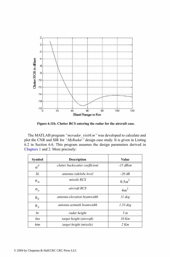
© 200
The MATLAB program myradar_visit6.m was developed to calculate and plot the CNR and SIR for MyRadar design case study. It is given in Listing 6.2 in Section 6.6. This program assumes the design parameters derived in Chapters 1 and 2. More precisely:
Symbol Description Value
clutter backscatter coefficient -15 dBsm
SL antenna sidelobe level -20 dB
missile RCS
aircraft RCS
antenna elevation beamwidth 11 deg
antenna azimuth beamwidth 1.33 deg
hr radar height 5 m
hta target height (aircraft) 10 Km
htm target height (missile) 2 Km
Figure 6.11b. Clutter RCS entering the radar for the aircraft case.
σ0
σm 0.5m2
σa 4m2
θE
θA
4 by Chapman & Hall/CRC CRC Press LLC
© 200
Figure 6.12 shows a plot of the CNR and the SIR associated with the mis-sile. Figure 6.13 is similar to Fig. 6.12 except it is for the aircraft case. It is clear from these figures that the required SIR has been degraded significantly for the missile case and not as much for the aircraft case. This should not be surprising, since the missiles altitude is much smaller than that of the aircraft. Without clutter mitigation, the missile would not be detected at all. Alterna-tively, the aircraft detection is compromised at . Clutter mitigation is the subject of the next chapter.
radar peak power 20 KW
radar operating frequency 3GHz
effective noise temperature 290 degrees Kelvin
noise figure 6 dB
L radar total losses 8 dB
Uncompressed pulsewidth 20 microseconds
Symbol Description Value
Pt
f0
T0
F
τ′
R 80Km≤
Figure 6.12. SNR, CNR, and SIR versus range for the missile case.
4 by Chapman & Hall/CRC CRC Press LLC
© 200
6.6. MATLAB Program and Function ListingsThis section presents listings for all MATLAB programs/functions used in
this chapter. The user is advised to rerun these programs with different input parameters.
Listing 6.1. MATALB Function clutter_rcs.mfunction [sigmaC,CNR] = clutter_rcs(sigma0, thetaE, thetaA, SL, range, hr, ht, pt, f0, b, t0, f, l,ant_id)% This function calculates the clutter RCS and the CNR for a ground based radar.clight = 3.e8; % speed of light in meters per secondlambda = clight /f0;thetaA_deg = thetaA;thetaE_deg = thetaE;thetaA = thetaA_deg * pi /180; % antenna azimuth beamwidth in radiansthetaE = thetaE_deg * pi /180.; % antenna elevation beamwidth in radiansre = 6371000; % earth radius in metersrh = sqrt(8.0*hr*re/3.); % range to horizon in meters
Figure 6.13. SNR, CNR and SIR versus range for the aircraft case.
4 by Chapman & Hall/CRC CRC Press LLC
© 200
SLv = 10.0^(SL/10); % radar rms sidelobes in voltssigma0v = 10.0^(sigma0/10); % clutter backscatter coefficient tau = 1/b; % pulsewidth deltar = clight * tau / 2.; % range resolution for unmodulated pulse%%%%%%%%%%%%%%%%%%%%%%%%%%%%%%range_m = 1000 .* range; % range in meters%%%%%%%%%%%%%%%%%%%%%%%%%%%%%%thetar = asin(hr ./ range_m);thetae = asin((ht-hr) ./ range_m);propag_atten = 1. + ((range_m ./ rh).^4); % propagation attenuation due to round earthRg = range_m .* cos(thetar);deltaRg = deltar .* cos(thetar);theta_sum = thetae + thetar;% use sinc^2 antenna pattern when ant_id=1% use Gaussian antenna pattern when ant_id=2if(ant_id ==1) % use sinc^2 antenna pattern ant_arg = (2.78 * theta_sum ) ./ (pi*thetaE); gain = (sinc(ant_arg)).^2;else gain = exp(-2.776 .*(theta_sum./thetaE).^2);end% compute sigmacsigmac = (sigma0v .* Rg .* deltaRg) .* (pi * SLv * SLv + thetaA .* gain.^2) ./ propag_atten;sigmaC = 10*log10(sigmac);%%%%%%%%%%%%%%%%%%%%%%%%%%%%%%%%%%%if (size(range,2)==1) fprintf('Sigma_Clutter='); sigmaCelse figure(1) plot(range, sigmaC) grid xlabel('Slant Range in Km') ylabel('Clutter RCS in dBsm')end%%%%%%%%%%%%%%%%%%%%%%%%%%%%%%%%%% Calculate CNRpt = pt * 1000;g = 26000 / (thetaA_deg*thetaE_deg); % antenna gainF = 10.^(f/10); % noise figure is 6 dBLt = 10.^(l/10); % total radar losses 13 dBk = 1.38e-23; % Boltzmans constantT0 = t0; % noise temperature 290K
4 by Chapman & Hall/CRC CRC Press LLC
© 200
argnumC = 10*log10(pt*g*g*lambda*lambda*tau .* sigmac);argdem = 10*log10(((4*pi)^3)*k*T0*Lt*F .*(range_m).^4);CNR = argnumC - argdem;%%%%%%%%%%%%%%%%%%%%%%%%%%%%%%%if (size(range,2) ==1) fprintf('Cluuter_to_Noise_ratio='); CNR else figure(2) plot(range, CNR,'r') grid xlabel('Slant Range in Km') ylabel('CNR in dB') end
Listing 6.2. MATLAB Program myradar_visit6.mclear allclose allthetaA= 1.33; % antenna azimuth beamwidth in degreesthetaE = 11; % antenna elevation beamwidth in degreeshr = 5.; % radar height to center of antenna (phase reference) in metershtm = 2000.; % target (missile) high in metershta = 10000.; % target (aircraft) high in metersSL = -20; % radar rms sidelobes in dBsigma0 = -15; % clutter backscatter coefficient b = 1.0e6; %1-MHz bandwidth t0 = 290; % noise temperature 290 degrees Kelvinf0 = 3e9; % 3 GHz center frequencypt = 114.6; % radar peak power in KWf = 6; % 6 dB noise figurel = 8; % 8 dB radar lossesrange = linspace(25,120,500); % radar slant range 25 to 120 Km, 500 points% calculate the clutter RCS and the associated CNR for both targets[sigmaCa,CNRa] = clutter_rcs(sigma0, thetaE, thetaA, SL, range, hr, hta, pt, f0, b, t0, f, l, 2);[sigmaCm,CNRm] = clutter_rcs(sigma0, thetaE, thetaA, L, range, hr, htm, pt, f0, b, t0, f, l, 2);close all%%%%%%%%%%%%%%%%%%%%%%%%np = 4;pfa = 1e-7;pdm = 0.99945;pda = 0.99812;% calculate the improvement factor
4 by Chapman & Hall/CRC CRC Press LLC
© 200
Im = improv_fac(np,pfa, pdm);Ia = improv_fac(np, pfa, pda);% calculate the integration lossLm = 10*log10(np) - Im;La = 10*log10(np) - Ia;pt = pt * 1000; % peak power in wattsrange_m = 1000 .* range; % range in metersg = 34.5139; % antenna gain in dBsigmam = 0.5; % missile RCS m squaredsigmaa = 4; % aircraft RCS m squarednf = f; %noise figure in dBloss = l; % radar losses in dBlosstm = loss + Lm; % total loss for missilelossta = loss + La; % total loss for aircraft% modify pt by np*pt to account for pulse integrationSNRm = radar_eq(np*pt, f0, g, sigmam, t0, b, nf, losstm, range_m);SNRa = radar_eq(np*pt, f0, g, sigmaa, t0, b, nf, lossta, range_m);snrm = 10.^(SNRm./10);snra = 10.^(SNRa./10);cnrm = 10.^(CNRm./10);cnra = 10.^(CNRa./10);SIRm = 10*log10(snrm ./ (1+cnrm));SIRa = 10*log10(snra ./ (1+cnra));%%%%%%%%%%%%%%%%%%%%%%%%%%%%%%%figure(3)plot(range, SNRm,'k', range, CNRm,'k :', range,SIRm,'k -.')gridlegend('Desired SNR; from Chapter 5','CNR','SIR')xlabel('Slant Range in Km')ylabel('dB')title('Missile case; 21-frame cumulative detection')%%%%%%%%%%%%%%%%%%%%%%%%%%%%%%%%%%%%%%%%%%figure(4)plot(range, SNRa,'k', range, CNRa,'k :', range,SIRa,'k -.')gridlegend('Desired SNR; from Chapter 5','CNR','SIR')xlabel('Slant Range in Km')ylabel('dB')title('Aircraft case; 21-frame cumulative detection')
4 by Chapman & Hall/CRC CRC Press LLC
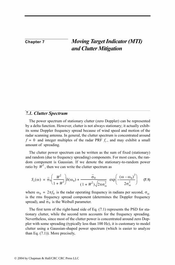
© 200
Chapter 7 Moving Target Indicator (MTI) and Clutter Mitigation
7.1. Clutter SpectrumThe power spectrum of stationary clutter (zero Doppler) can be represented
by a delta function. However, clutter is not always stationary; it actually exhib-its some Doppler frequency spread because of wind speed and motion of the radar scanning antenna. In general, the clutter spectrum is concentrated around
and integer multiples of the radar PRF , and may exhibit a small amount of spreading.
The clutter power spectrum can be written as the sum of fixed (stationary) and random (due to frequency spreading) components. For most cases, the ran-dom component is Gaussian. If we denote the stationary-to-random power ratio by , then we can write the clutter spectrum as
(7.1)
where is the radar operating frequency in radians per second, is the rms frequency spread component (determines the Doppler frequency spread), and is the Weibull parameter.
The first term of the right-hand side of Eq. (7.1) represents the PSD for sta-tionary clutter, while the second term accounts for the frequency spreading. Nevertheless, since most of the clutter power is concentrated around zero Dop-pler with some spreading (typically less than 100 Hz), it is customary to model clutter using a Gaussian-shaped power spectrum (which is easier to analyze than Eq. (7.1)). More precisely,
f 0= fr
W2
Sc ω( ) σ0W2
1 W2+----------------
δ ω0( )σ0
1 W2+( ) 2πσω2
--------------------------------------- ω ω0( )2
2σω2
-----------------------
exp+=
ω0 2πf0= σω
σ0
4 by Chapman & Hall/CRC CRC Press LLC
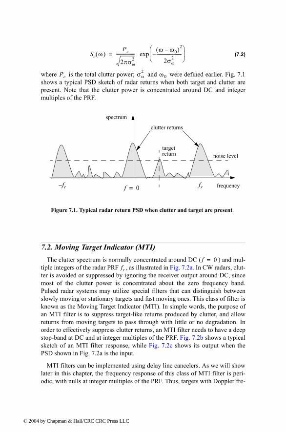
© 200
(7.2)
where is the total clutter power; and were defined earlier. Fig. 7.1 shows a typical PSD sketch of radar returns when both target and clutter are present. Note that the clutter power is concentrated around DC and integer multiples of the PRF.
7.2. Moving Target Indicator (MTI)The clutter spectrum is normally concentrated around DC ( ) and mul-
tiple integers of the radar PRF , as illustrated in Fig. 7.2a. In CW radars, clut-ter is avoided or suppressed by ignoring the receiver output around DC, since most of the clutter power is concentrated about the zero frequency band. Pulsed radar systems may utilize special filters that can distinguish between slowly moving or stationary targets and fast moving ones. This class of filter is known as the Moving Target Indicator (MTI). In simple words, the purpose of an MTI filter is to suppress target-like returns produced by clutter, and allow returns from moving targets to pass through with little or no degradation. In order to effectively suppress clutter returns, an MTI filter needs to have a deep stop-band at DC and at integer multiples of the PRF. Fig. 7.2b shows a typical sketch of an MTI filter response, while Fig. 7.2c shows its output when the PSD shown in Fig. 7.2a is the input.
MTI filters can be implemented using delay line cancelers. As we will show later in this chapter, the frequency response of this class of MTI filter is peri-odic, with nulls at integer multiples of the PRF. Thus, targets with Doppler fre-
Sc ω( )Pc
2πσω2
----------------- ω ω0( )2
2σω2
-----------------------
exp=
Pc σω2 ω0
frequencyfrf 0=fr
targetreturn
spectrum
noise level
clutter returns
Figure 7.1. Typical radar return PSD when clutter and target are present.
f 0=fr
4 by Chapman & Hall/CRC CRC Press LLC
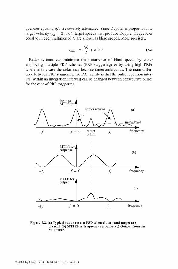
© 200
quencies equal to are severely attenuated. Since Doppler is proportional to target velocity ( ), target speeds that produce Doppler frequencies equal to integer multiples of are known as blind speeds. More precisely,
(7.3)
Radar systems can minimize the occurrence of blind speeds by either employing multiple PRF schemes (PRF staggering) or by using high PRFs where in this case the radar may become range ambiguous. The main differ-ence between PRF staggering and PRF agility is that the pulse repetition inter-val (within an integration interval) can be changed between consecutive pulses for the case of PRF staggering.
nfrfd 2v λ⁄=
fr
vblindλfr
2------- n 0≥;=
noise level
frequencytargetreturn
frf 0=fr
clutter returns
MTI filterresponse
frequencyfrf 0=fr
input to MTI filter
MTI filteroutput
frequencyfrf 0=fr
(a)
(c)
(b)
Figure 7.2. (a) Typical radar return PSD when clutter and target are present. (b) MTI filter frequency response. (c) Output from an MTI filter.
4 by Chapman & Hall/CRC CRC Press LLC
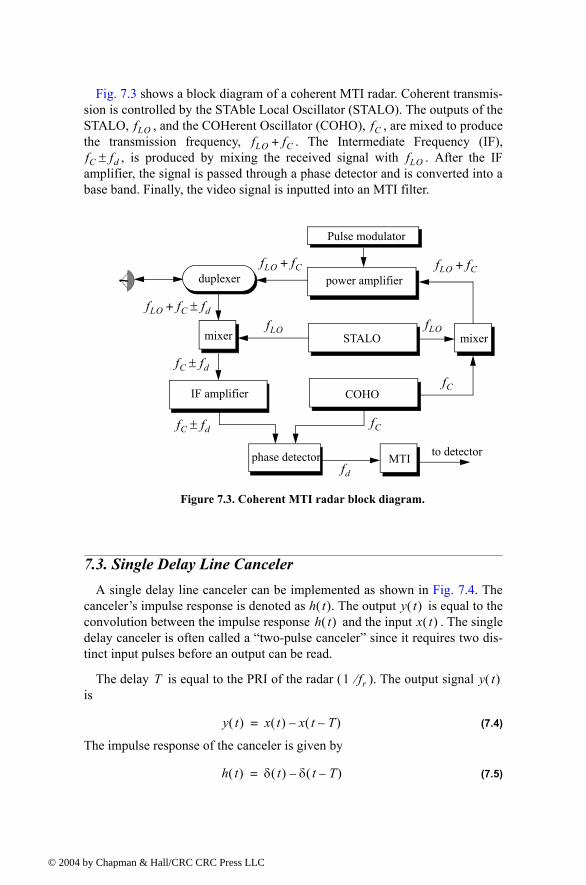
© 200
Fig. 7.3 shows a block diagram of a coherent MTI radar. Coherent transmis-sion is controlled by the STAble Local Oscillator (STALO). The outputs of the STALO, , and the COHerent Oscillator (COHO), , are mixed to produce the transmission frequency, . The Intermediate Frequency (IF),
, is produced by mixing the received signal with . After the IF amplifier, the signal is passed through a phase detector and is converted into a base band. Finally, the video signal is inputted into an MTI filter.
7.3. Single Delay Line CancelerA single delay line canceler can be implemented as shown in Fig. 7.4. The
cancelers impulse response is denoted as . The output is equal to the convolution between the impulse response and the input . The single delay canceler is often called a two-pulse canceler since it requires two dis-tinct input pulses before an output can be read.
The delay is equal to the PRI of the radar ( ). The output signal is
(7.4)
The impulse response of the canceler is given by
(7.5)
fLO fCfLO fC+
fC fd± fLO
Pulse modulator
duplexer power amplifier
mixer mixerSTALO
COHOIF amplifier
phase detector MTI to detector
fLO fC+
fLO
fLO fC fd±+
fC
fLO fC+
fLO
fC
fC fd±
fd
fC fd±
Figure 7.3. Coherent MTI radar block diagram.
h t( ) y t( )h t( ) x t( )
T 1 fr⁄ y t( )
y t( ) x t( ) x t T( )=
h t( ) δ t( ) δ t T( )=
4 by Chapman & Hall/CRC CRC Press LLC
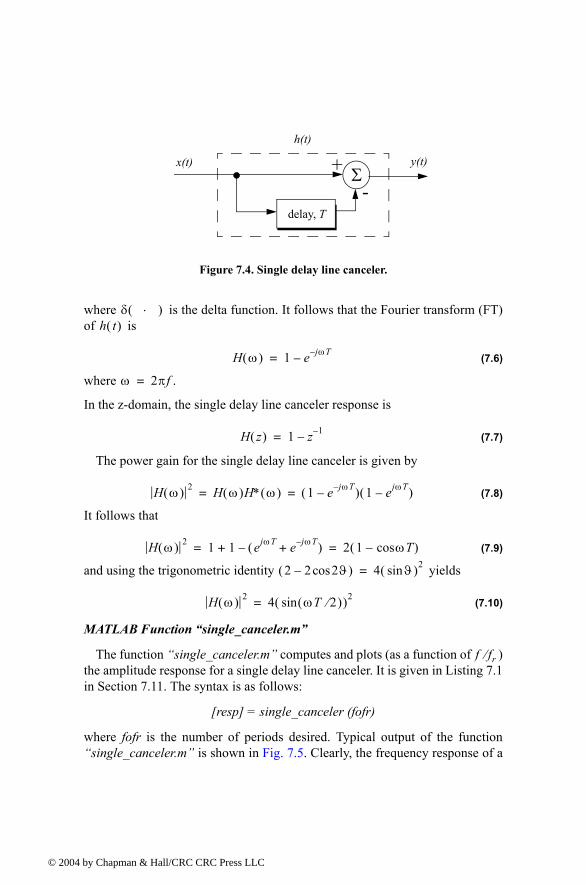
© 200
where is the delta function. It follows that the Fourier transform (FT) of is
(7.6)
where .
In the z-domain, the single delay line canceler response is
(7.7)
The power gain for the single delay line canceler is given by
(7.8)
It follows that
(7.9)
and using the trigonometric identity yields
(7.10)
MATLAB Function single_canceler.m
The function single_canceler.m computes and plots (as a function of ) the amplitude response for a single delay line canceler. It is given in Listing 7.1 in Section 7.11. The syntax is as follows:
[resp] = single_canceler (fofr)
where fofr is the number of periods desired. Typical output of the function single_canceler.m is shown in Fig. 7.5. Clearly, the frequency response of a
-+ Σ
x(t) y(t)
delay, T
h(t)
Figure 7.4. Single delay line canceler.
δ ⋅( )h t( )
H ω( ) 1 e jωT=
ω 2πf=
H z( ) 1 z 1=
H ω( ) 2 H ω( )H∗ ω( ) 1 e jωT( ) 1 ejωT( )= =
H ω( ) 2 1 1 ejωT e jωT+( )+ 2 1 ωTcos( )= =
2 2 2ϑcos( ) 4 ϑsin( )2=
H ω( ) 2 4 ωT 2⁄( )sin( )2=
f fr⁄
4 by Chapman & Hall/CRC CRC Press LLC
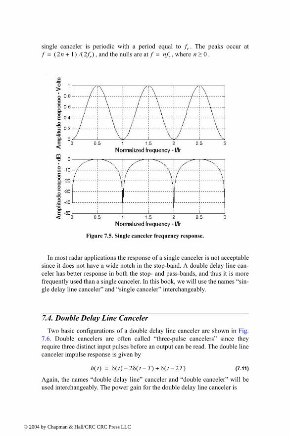
© 200
single canceler is periodic with a period equal to . The peaks occur at , and the nulls are at , where .
In most radar applications the response of a single canceler is not acceptable since it does not have a wide notch in the stop-band. A double delay line can-celer has better response in both the stop- and pass-bands, and thus it is more frequently used than a single canceler. In this book, we will use the names sin-gle delay line canceler and single canceler interchangeably.
7.4. Double Delay Line CancelerTwo basic configurations of a double delay line canceler are shown in Fig.
7.6. Double cancelers are often called three-pulse cancelers since they require three distinct input pulses before an output can be read. The double line canceler impulse response is given by
(7.11)
Again, the names double delay line canceler and double canceler will be used interchangeably. The power gain for the double delay line canceler is
frf 2n 1+( ) 2fr( )⁄= f nfr= n 0≥
Figure 7.5. Single canceler frequency response.
h t( ) δ t( ) 2δ t T( ) δ t 2T( )+=
4 by Chapman & Hall/CRC CRC Press LLC
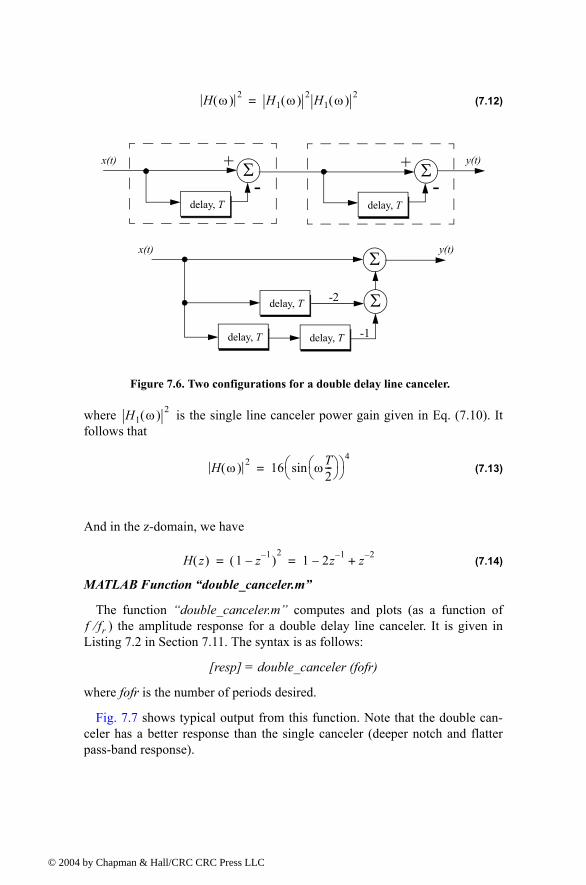
© 200
(7.12)
where is the single line canceler power gain given in Eq. (7.10). It follows that
(7.13)
And in the z-domain, we have
(7.14)
MATLAB Function double_canceler.m
The function double_canceler.m computes and plots (as a function of ) the amplitude response for a double delay line canceler. It is given in
Listing 7.2 in Section 7.11. The syntax is as follows:
[resp] = double_canceler (fofr)
where fofr is the number of periods desired.
Fig. 7.7 shows typical output from this function. Note that the double can-celer has a better response than the single canceler (deeper notch and flatter pass-band response).
H ω( ) 2 H1 ω( ) 2 H1 ω( ) 2=
-+ Σ
x(t) y(t)
delay, T-
+ Σ
delay, T
Σ
delay, T
Σdelay, T
delay, T
-2
-1
x(t) y(t)
Figure 7.6. Two configurations for a double delay line canceler.
H1 ω( ) 2
H ω( ) 2 16 ωT2---
sin
4=
H z( ) 1 z 1( )2
1 2z 1 z 2+= =
f fr⁄
4 by Chapman & Hall/CRC CRC Press LLC
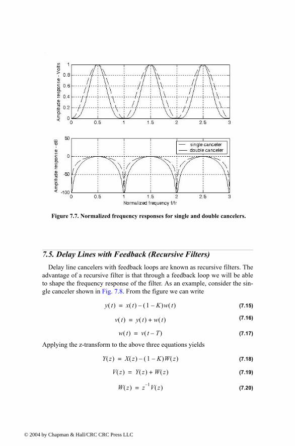
© 200
7.5. Delay Lines with Feedback (Recursive Filters)Delay line cancelers with feedback loops are known as recursive filters. The
advantage of a recursive filter is that through a feedback loop we will be able to shape the frequency response of the filter. As an example, consider the sin-gle canceler shown in Fig. 7.8. From the figure we can write
(7.15)
(7.16)
(7.17)
Applying the z-transform to the above three equations yields
(7.18)
(7.19)
(7.20)
Figure 7.7. Normalized frequency responses for single and double cancelers.
y t( ) x t( ) 1 K( )w t( )=
v t( ) y t( ) w t( )+=
w t( ) v t T( )=
Y z( ) X z( ) 1 K( )W z( )=
V z( ) Y z( ) W z( )+=
W z( ) z 1 V z( )=
4 by Chapman & Hall/CRC CRC Press LLC
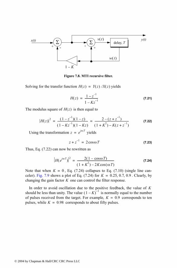
© 200
Solving for the transfer function yields
(7.21)
The modulus square of is then equal to
(7.22)
Using the transformation yields
(7.23)
Thus, Eq. (7.22) can now be rewritten as
(7.24)
Note that when , Eq. (7.24) collapses to Eq. (7.10) (single line can-celer). Fig. 7.9 shows a plot of Eq. (7.24) for . Clearly, by changing the gain factor one can control the filter response.
In order to avoid oscillation due to the positive feedback, the value of should be less than unity. The value is normally equal to the number of pulses received from the target. For example, corresponds to ten pulses, while corresponds to about fifty pulses.
Σ Σ delay, Tx(t) y(t)
+ - + +
w t( )
v t( )
1 K
Figure 7.8. MTI recursive filter.
H z( ) Y z( ) X z( )⁄=
H z( ) 1 z 1
1 Kz 1--------------------=
H z( )
H z( ) 2 1 z 1( ) 1 z( )
1 Kz 1( ) 1 Kz( )---------------------------------------------- 2 z z 1+( )
1 K2+( ) K z z 1+( )---------------------------------------------------= =
z ejωT=
z z 1+ 2 ωTcos=
H ejωT( )2 2 1 ωTcos( )
1 K2+( ) 2K ωT( )cos-------------------------------------------------------=
K 0=K 0.25 0.7 0.9, ,=
K
K1 K( ) 1
K 0.9=K 0.98=
4 by Chapman & Hall/CRC CRC Press LLC
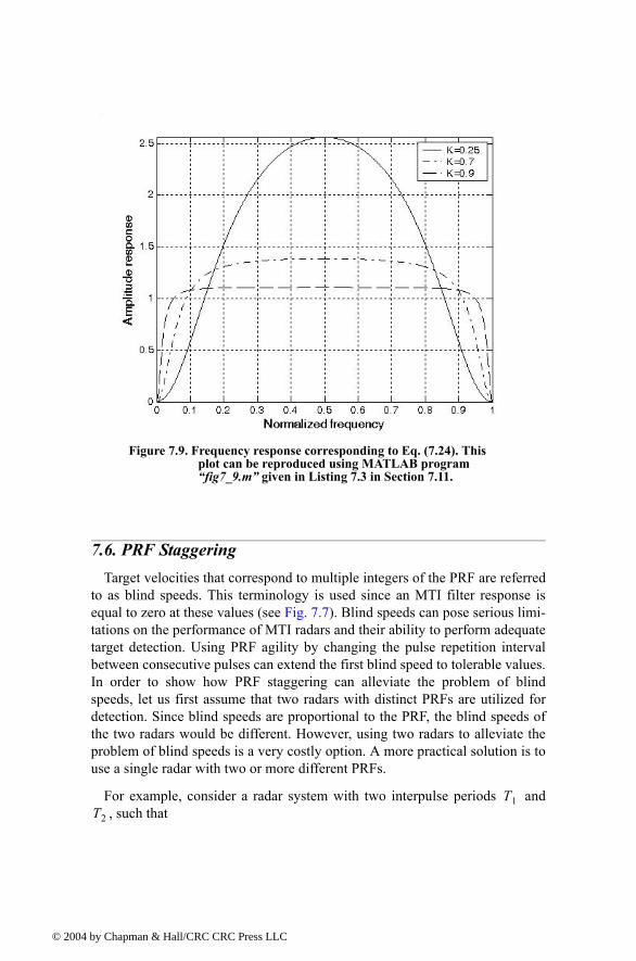
© 200
7.6. PRF StaggeringTarget velocities that correspond to multiple integers of the PRF are referred
to as blind speeds. This terminology is used since an MTI filter response is equal to zero at these values (see Fig. 7.7). Blind speeds can pose serious limi-tations on the performance of MTI radars and their ability to perform adequate target detection. Using PRF agility by changing the pulse repetition interval between consecutive pulses can extend the first blind speed to tolerable values. In order to show how PRF staggering can alleviate the problem of blind speeds, let us first assume that two radars with distinct PRFs are utilized for detection. Since blind speeds are proportional to the PRF, the blind speeds of the two radars would be different. However, using two radars to alleviate the problem of blind speeds is a very costly option. A more practical solution is to use a single radar with two or more different PRFs.
For example, consider a radar system with two interpulse periods and , such that
Figure 7.9. Frequency response corresponding to Eq. (7.24). This plot can be reproduced using MATLAB program fig7_9.m given in Listing 7.3 in Section 7.11.
T1T2
4 by Chapman & Hall/CRC CRC Press LLC
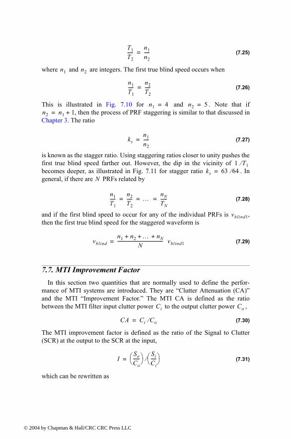
© 200
(7.25)
where and are integers. The first true blind speed occurs when
(7.26)
This is illustrated in Fig. 7.10 for and . Note that if , then the process of PRF staggering is similar to that discussed in
Chapter 3. The ratio
(7.27)
is known as the stagger ratio. Using staggering ratios closer to unity pushes the first true blind speed farther out. However, the dip in the vicinity of becomes deeper, as illustrated in Fig. 7.11 for stagger ratio . In general, if there are PRFs related by
(7.28)
and if the first blind speed to occur for any of the individual PRFs is , then the first true blind speed for the staggered waveform is
(7.29)
7.7. MTI Improvement FactorIn this section two quantities that are normally used to define the perfor-
mance of MTI systems are introduced. They are Clutter Attenuation (CA) and the MTI Improvement Factor. The MTI CA is defined as the ratio between the MTI filter input clutter power to the output clutter power ,
(7.30)
The MTI improvement factor is defined as the ratio of the Signal to Clutter (SCR) at the output to the SCR at the input,
(7.31)
which can be rewritten as
T1
T2-----
n1
n2-----=
n1 n2
n1
T1-----
n2
T2-----=
n1 4= n2 5=n2 n1 1+=
ksn1
n2-----=
1 T1⁄ks 63 64⁄=
N
n1
T1-----
n2
T2----- …
nN
TN------= = =
vblind1
vblindn1 n2 … nN+ + +
N----------------------------------------- vblind1=
Ci Co
CA Ci Co⁄=
ISo
Co------ Si
Ci----- ⁄=
4 by Chapman & Hall/CRC CRC Press LLC
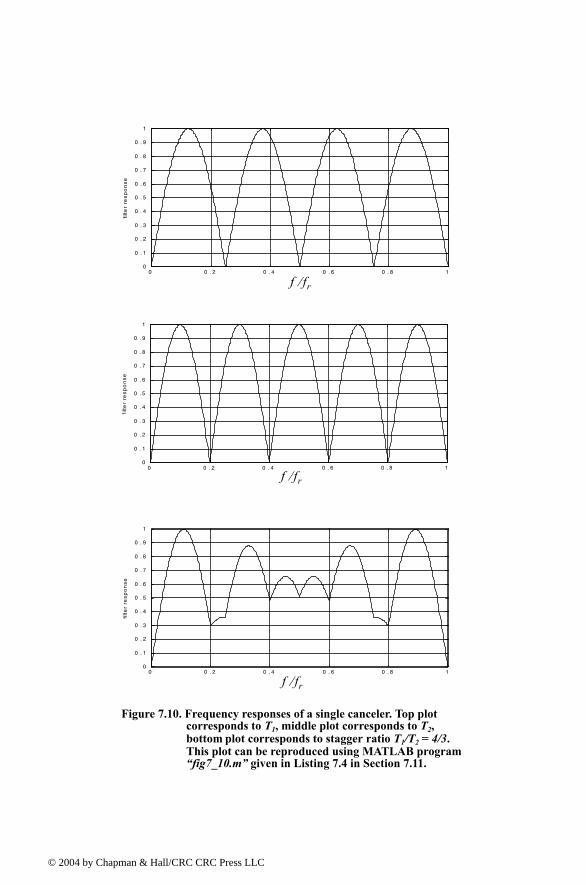
© 200
0 0 . 2 0 . 4 0 . 6 0 . 8 10
0 . 1
0 . 2
0 . 3
0 . 4
0 . 5
0 . 6
0 . 7
0 . 8
0 . 9
1fi
lte
r re
sp
on
se
0 0 . 2 0 . 4 0 . 6 0 . 8 10
0 . 1
0 . 2
0 . 3
0 . 4
0 . 5
0 . 6
0 . 7
0 . 8
0 . 9
1
filt
er
res
po
ns
e
0 0 . 2 0 . 4 0 . 6 0 . 8 10
0 . 1
0 . 2
0 . 3
0 . 4
0 . 5
0 . 6
0 . 7
0 . 8
0 . 9
1
filt
er
res
po
ns
e
f fr⁄
f fr⁄
f fr⁄
Figure 7.10. Frequency responses of a single canceler. Top plot corresponds to T1, middle plot corresponds to T2, bottom plot corresponds to stagger ratio T1/T2 = 4/3. This plot can be reproduced using MATLAB program fig7_10.m given in Listing 7.4 in Section 7.11.
4 by Chapman & Hall/CRC CRC Press LLC
© 200
(7.32)
The ratio is the average power gain of the MTI filter, and it is equal to . In this section, a closed form expression for the improvement factor
using a Gaussian-shaped power spectrum is developed. A Gaussian-shaped clutter power spectrum is given by
0 5 1 0 1 5 2 0 2 5 3 0- 4 0
- 3 5
- 3 0
- 2 5
- 2 0
- 1 5
- 1 0
- 5
0fil
ter r
espo
nse,
dB
target velocity relative to first blind speed; 63/64
0 2 4 6 8 1 0 1 2 1 4 1 6- 4 0
- 3 5
- 3 0
- 2 5
- 2 0
- 1 5
- 1 0
- 5
0
target velocity relative to first blind speed; 33/34
filte
r res
pons
e, d
B
Figure 7.11. MTI responses, staggering ratio 63/64. This plot can be reproduced using MATLAB program fig7_11.m given in Listing 7.5 in Section 7.11.
ISo
Si-----CA=
So Si⁄H ω( ) 2
4 by Chapman & Hall/CRC CRC Press LLC
© 200
(7.33)
where is the clutter power (constant), and is the clutter rms frequency (which describes the clutter spectrum spread in the frequency domain). It is given by
(7.34)
is the standard deviation for the clutter spectrum spread due to wind veloc-ity; is the standard deviation for the clutter spectrum spread due to antenna scanning; and is the standard deviation for the clutter spectrum spread due to the radar platform motion (if applicable). It can be shown that1
(7.35)
(7.36)
(7.37)
where is the wavelength and is the wind rms velocity; is the antenna 3-db azimuth beamwidth (in radians); is the antenna scan time; is the platform velocity; and is the azimuth angle (in radians) relative to the direc-tion of motion.
The clutter power at the input of an MTI filter is
(7.38)
Factoring out the constant yields
(7.39)
It follows that
1. Berkowtiz, R. S., Modern Radar, Analysis, Evaluation, and System Deign, John Wiley & Sons, New York, 1965.
W f( )Pc
2π σt
------------------- f2 2σt2⁄( )exp=
Pc σt
σt σv2 σs
2 σw2+ +=
σvσs
σv
σv2σw
λ----------=
σs 0.265 2πΘaTscan------------------- =
σsvλ--- θsin≈
λ σw ΘaTscan v
θ
CiPc
2π σt
------------------- f2
2σt2
---------
exp fd
∞
∞
∫=
Pc
Ci Pc1
2πσt
---------------- f2
2σt2
---------
exp fd
∞
∞
∫=
4 by Chapman & Hall/CRC CRC Press LLC
© 200
(7.40)
The clutter power at the output of an MTI is
(7.41)
7.7.1. Two-Pulse MTI Case
In this section we will continue the analysis using a single delay line can-celer. The frequency response for a single delay line canceler is given by Eq. (7.6). The single canceler power gain is given in Eq. (7.10), which will be repeated here, in terms of rather than , as Eq. (7.42),
(7.42)
It follows that
(7.43)
Now, since clutter power will only be significant for small , then the ratio is very small (i.e., ). Consequently, by using the small angle
approximation, Eq. (7.43) is approximated by
(7.44)
which can be rewritten as
(7.45)
The integral part in Eq. (7.45) is the second moment of a zero mean Gaussian distribution with variance . Replacing the integral in Eq. (7.45) by yields
(7.46)
Substituting Eqs. (7.46) and (7.40) into Eq. (7.30) produces
Ci Pc=
Co W f( ) H f( ) 2 fd
∞
∞
∫=
f ω
H f( ) 2 4 πffr----- sin
2=
CoPc
2π σt
------------------- f2
2σt2
---------
exp 4 πffr----- sin
2fd
∞
∞
∫=
ff fr⁄ σt fr«
CoPc
2π σt
------------------- f2
2σt2
---------
exp 4 πffr----- 2
fd
∞
∞
∫≈
Co4Pcπ
2
fr2
--------------- 1
2πσt2
----------------- f2
2σt2
---------
exp f2 fd
∞
∞
∫=
σt2 σt
2
Co4Pcπ
2
fr2
--------------- σt2=
4 by Chapman & Hall/CRC CRC Press LLC
© 200
(7.47)
It follows that the improvement factor for a single canceler is
(7.48)
The power gain ratio for a single canceler is (remember that is periodic with period )
(7.49)
Using the trigonometric identity yields
(7.50)
It follows that
(7.51)
The expression given in Eq. (7.51) is an approximation valid only for . When the condition is not true, then the autocorrelation func-
tion needs to be used in order to develop an exact expression for the improve-ment factor.
Example:
A certain radar has . If the clutter rms is (wooded hills with ), find the improvement factor when a single delay line canceler is used.
Solution:
In this case . It follows that the clutter attenuation CA is
and since we get
.
CACi
Co------
fr
2πσt------------
2= =
Ifr
2πσt------------
2 So
Si-----=
H f( )fr
So
Si----- H f( ) 2 1
fr--- 4 πf
fr-----sin
2fd
fr 2⁄
fr 2⁄
∫= =
2 2 2ϑcos( ) 4 ϑsin( )2=
H f( ) 2 1fr--- 2 2 2πf
fr--------cos
fd
fr 2⁄
fr 2⁄
∫ 2= =
I 2fr
2πσt------------
2=
σt fr« σt fr«
fr 800Hz= σv 6.4Hz=σw 1.16311Km hr⁄=
σt σv=
CAfr
2πσt------------
2 8002π( ) 6.4( )
------------------------
2395.771 25.974dB= = = =
So Si⁄ 2 3dB= =
IdB CA So Si⁄+( )dB 3 25.97+ 28.974dB= = =
4 by Chapman & Hall/CRC CRC Press LLC
© 200
7.7.2. The General Case
A general expression for the improvement factor for the n-pulse MTI (shown for a 2-pulse MTI in Eq. (7.51)) is given by
(7.52)
where the double factorial notation is defined by
(7.53)
(7.54)
Of course ; is defined by
(7.55)
where are the Binomial coefficients for the MTI filter. It follows that for a 2-pulse, 3-pulse, and 4-pulse MTI are respectively
(7.56)
Using this notation, then the improvement factor for a 3-pulse and 4-pulse MTI are respectively given by
(7.57)
(7.58)
7.8. MyRadar Design Case Study - Visit 7
7.8.1. Problem Statement
The impact of surface clutter on the MyRadar design case study was ana-lyzed. Assume that the wind rms velocity . Propose a clutter mitigation process utilizing a 2-pulse and a 3-pulse MTI. All other parameters are as calculated in the previous chapters.
I 1Q2 2 n 1( ) 1( )!!---------------------------------------------
fr
2πσt------------
2 n 1( )=
2n 1( )!! 1 3 5× …× 2n 1( )××=
2n( )!! 2 4 … 2n×××=
0!! 1= Q
Q2 1
Ai2
i 1=
n
∑---------------=
Ai Q2
12--- 1
20------ 1
70------, ,
I3 pulse 2fr
2πσt------------
4=
I4 pulse43---
fr
2πσt------------
6=
σw 0.45m s⁄=
4 by Chapman & Hall/CRC CRC Press LLC
© 200
7.8.2. A Design
In earlier chapters we determined that the wavelength is , the PRF is , the scan rate is , and the antenna azimuth 3-db beamwidth is . It follows that
(7.59)
(7.60)
Thus, the total clutter rms spectrum spread is
(7.61)
The expected clutter attenuation using a 2-pulse and a 3-pulse MTI are respectively given by
(7.62)
(7.63)
To demonstrate the effect of a 2-pulse and 3-pulse MTI on MyRadar design case study, the MATLAB program myradar_visit7.m has been devel-oped. It is given in Listing 7.6 in Section 7.5. This program utilizes the radar equation with pulse compression. In this case, the peak power was established in Chapter 5 as . Figs. 7.12 and 7.13 show the desired SNR and the calculated SIR using a 2-pulse and a 3-pulse MTI filter respectively, for the missile case. Figs. 7.14 and 7.15 show similar output for the aircraft case.
One may argue, depending on the tracking scheme adopted by the radar, that for a tracking radar
(7.64)
since for a radar that employes a monopulse tracking option. In this design, we will assume a Kalman filter tracker. For more details the reader is advised to visit Chapter 9.
λ 0.1m=fr 1KHz= Tscan 2s=
Θa 1.3°=
σv2σw
λ---------- 2 0.45×
0.1------------------- 9Hz= = =
σs 0.265 2πΘaTscan------------------- 0.265 2 π×
1.32 π180--------- 2××
-----------------------------------× 36.136Hz= = =
σt σv2 σs
2+ 81 1305.810+ 1386.810 37.24Hz= = = =
I2pulse 2fr
2πσt------------
22 1000
2 π 37.24××--------------------------------
2× 36.531W
W----- 15.63dB⇒= = =
I3pulse 2fr
2πσt------------
42 1000
2 π 37.24××--------------------------------
4× 667.247W
W----- 28.24dB⇒= = =
Pt 10KW≤
σt σv 9Hz= =
σs 0=
4 by Chapman & Hall/CRC CRC Press LLC
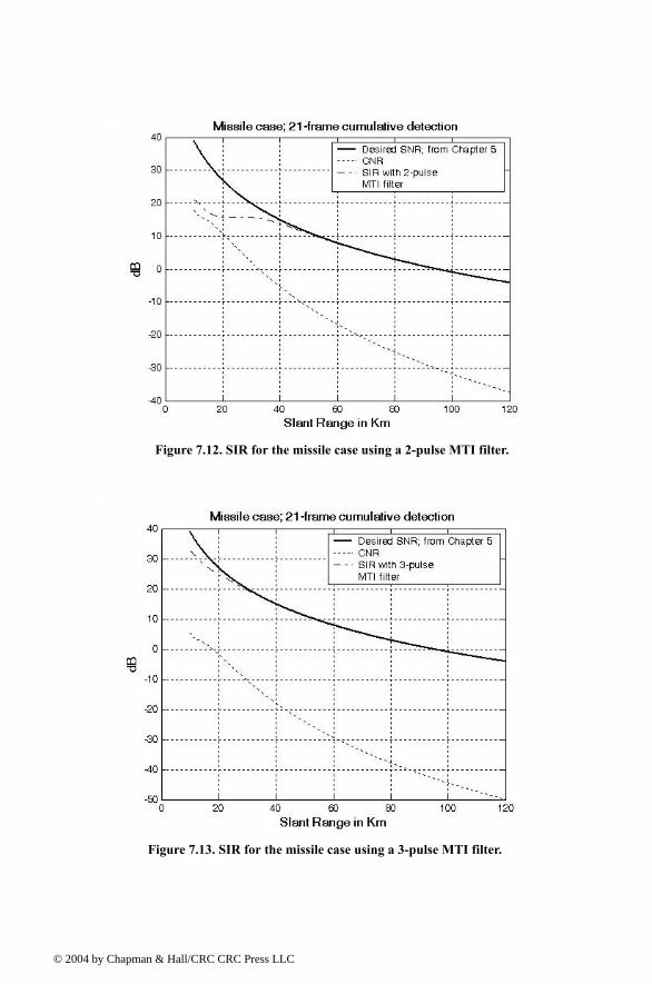
© 200
Figure 7.12. SIR for the missile case using a 2-pulse MTI filter.
Figure 7.13. SIR for the missile case using a 3-pulse MTI filter.
4 by Chapman & Hall/CRC CRC Press LLC
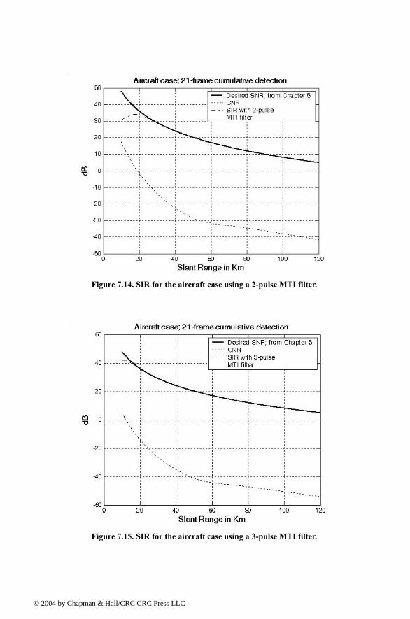
© 200
Figure 7.14. SIR for the aircraft case using a 2-pulse MTI filter.
Figure 7.15. SIR for the aircraft case using a 3-pulse MTI filter.
4 by Chapman & Hall/CRC CRC Press LLC
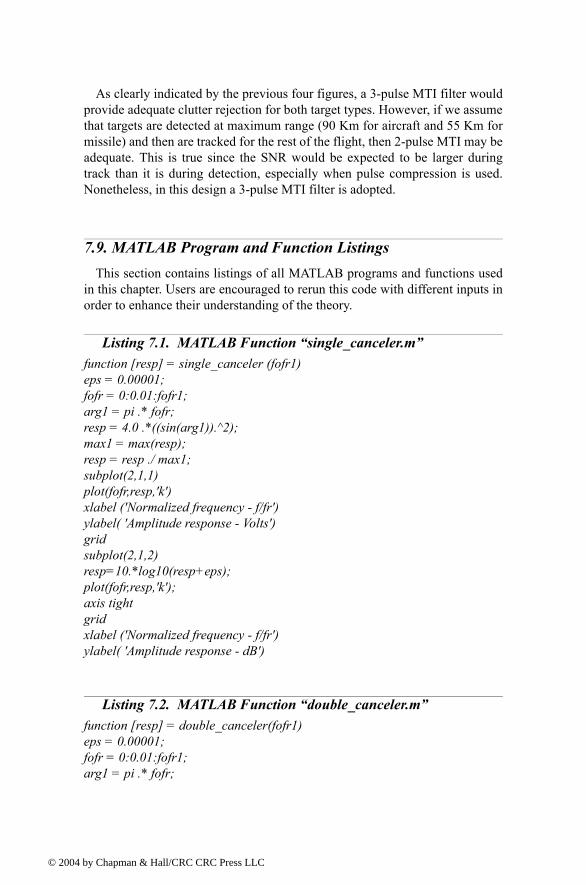
© 200
As clearly indicated by the previous four figures, a 3-pulse MTI filter would provide adequate clutter rejection for both target types. However, if we assume that targets are detected at maximum range (90 Km for aircraft and 55 Km for missile) and then are tracked for the rest of the flight, then 2-pulse MTI may be adequate. This is true since the SNR would be expected to be larger during track than it is during detection, especially when pulse compression is used. Nonetheless, in this design a 3-pulse MTI filter is adopted.
7.9. MATLAB Program and Function ListingsThis section contains listings of all MATLAB programs and functions used
in this chapter. Users are encouraged to rerun this code with different inputs in order to enhance their understanding of the theory.
Listing 7.1. MATLAB Function single_canceler.mfunction [resp] = single_canceler (fofr1)eps = 0.00001;fofr = 0:0.01:fofr1;arg1 = pi .* fofr;resp = 4.0 .*((sin(arg1)).^2);max1 = max(resp);resp = resp ./ max1;subplot(2,1,1)plot(fofr,resp,'k')xlabel ('Normalized frequency - f/fr')ylabel( 'Amplitude response - Volts')gridsubplot(2,1,2)resp=10.*log10(resp+eps);plot(fofr,resp,'k');axis tightgridxlabel ('Normalized frequency - f/fr')ylabel( 'Amplitude response - dB')
Listing 7.2. MATLAB Function double_canceler.mfunction [resp] = double_canceler(fofr1)eps = 0.00001;fofr = 0:0.01:fofr1;arg1 = pi .* fofr;
4 by Chapman & Hall/CRC CRC Press LLC
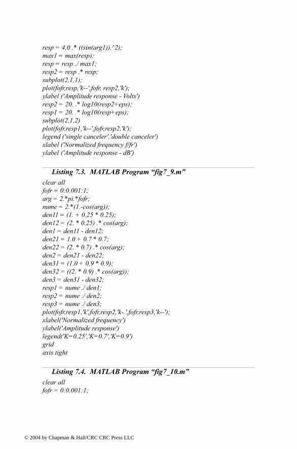
© 200
resp = 4.0 .* ((sin(arg1)).^2);max1 = max(resp);resp = resp ./ max1;resp2 = resp .* resp;subplot(2,1,1);plot(fofr,resp,'k--',fofr, resp2,'k');ylabel ('Amplitude response - Volts')resp2 = 20. .* log10(resp2+eps);resp1 = 20. .* log10(resp+eps);subplot(2,1,2)plot(fofr,resp1,'k--',fofr,resp2,'k');legend ('single canceler','double canceler')xlabel ('Normalized frequency f/fr')ylabel ('Amplitude response - dB')
Listing 7.3. MATLAB Program fig7_9.mclear allfofr = 0:0.001:1;arg = 2.*pi.*fofr;nume = 2.*(1.-cos(arg));den11 = (1. + 0.25 * 0.25);den12 = (2. * 0.25) .* cos(arg);den1 = den11 - den12;den21 = 1.0 + 0.7 * 0.7;den22 = (2. * 0.7) .* cos(arg);den2 = den21 - den22;den31 = (1.0 + 0.9 * 0.9);den32 = ((2. * 0.9) .* cos(arg));den3 = den31 - den32;resp1 = nume ./ den1;resp2 = nume ./ den2;resp3 = nume ./ den3;plot(fofr,resp1,'k',fofr,resp2,'k-.',fofr,resp3,'k--');xlabel('Normalized frequency')ylabel('Amplitude response')legend('K=0.25','K=0.7','K=0.9')gridaxis tight
Listing 7.4. MATLAB Program fig7_10.mclear allfofr = 0:0.001:1;
4 by Chapman & Hall/CRC CRC Press LLC
© 200
f1 = 4.0 .* fofr;f2 = 5.0 .* fofr;arg1 = pi .* f1;arg2 = pi .* f2;resp1 = abs(sin(arg1));resp2 = abs(sin(arg2));resp = resp1+resp2;max1 = max(resp);resp = resp./max1;plot(fofr,resp1,fofr,resp2,fofr,resp);xlabel('Normalized frequency f/fr')ylabel('Filter response')
Listing 7.5. MATLAB Program fig7_11.mclear allfofr = 0.01:0.001:32;a = 63.0 / 64.0;term1 = (1. - 2.0 .* cos(a*2*pi*fofr) + cos(4*pi*fofr)).^2;term2 = (-2. .* sin(a*2*pi*fofr) + sin(4*pi*fofr)).^2;resp = 0.25 .* sqrt(term1 + term2);resp = 10. .* log(resp);plot(fofr,resp);axis([0 32 -40 0]);grid
Listing 7.6. MATLAB Program myradar_visit7.mclear allclose allclutter_attenuation = 28.24;thetaA= 1.33; % antenna azimuth beamwidth in degreesthetaE = 11; % antenna elevation beamwidth in degreeshr = 5.; % radar height to center of antenna (phase reference) in metershtm = 2000.; % target (missile) height in metershta = 10000.; % target (aircraft) height in metersSL = -20; % radar rms sidelobes in dBsigma0 = -15; % clutter backscatter coefficient in dBb = 1.0e6; %1-MHz bandwidth t0 = 290; % noise temperature 290 degrees Kelvinf0 = 3e9; % 3 GHz center frequencypt = 114.6; % radar peak power in KWf = 6; % 6 dB noise figurel = 8; % 8 dB radar losses
4 by Chapman & Hall/CRC CRC Press LLC
© 200
range = linspace(25,120,500); % radar slant range 25 to 120 Km, 500 points% calculate the clutter RCS and the associated CNR for both targets[sigmaCa,CNRa] = clutter_rcs(sigma0, thetaE, thetaA, SL, range, hr, hta, pt, f0, b, t0, f, l,2);[sigmaCm,CNRm] = clutter_rcs(sigma0, thetaE, thetaA, SL, range, hr, htm, pt, f0, b, t0, f, l,2);close all%%%%%%%%%%%%%%%%%%%%%%%%np = 4;pfa = 1e-7;pdm = 0.99945;pda = 0.99812;% calculate the improvement factorIm = improv_fac(np,pfa, pdm);Ia = improv_fac(np, pfa, pda);% caculate the integration lossLm = 10*log10(np) - Im;La = 10*log10(np) - Ia;pt = pt * 1000; % peak power in wattsrange_m = 1000 .* range; % range in metersg = 34.5139; % antenna gain in dBsigmam = 0.5; % missile RCS m squaredsigmaa = 4; % aircraft RCS m squarednf = f; %noise figure in dBloss = l; % radar losses in dBlosstm = loss + Lm; % total loss for missilelossta = loss + La; % total loss for aircraft% modify pt by np*pt to account for pulse integrationSNRm = radar_eq(np*pt, f0, g, sigmam, t0, b, nf, losstm, range_m);SNRa = radar_eq(np*pt, f0, g, sigmaa, t0, b, nf, lossta, range_m);snrm = 10.^(SNRm./10);snra = 10.^(SNRa./10);CNRm = CNRm - clutter_attenuation;CNRa = CNRa - clutter_attenuation;cnrm = 10.^(CNRm./10);cnra = 10.^(CNRa./10);SIRm = 10*log10(snrm ./ (1+cnrm));SIRa = 10*log10(snra ./ (1+cnra));%%%%%%%%%%%%%%%%%%%%%%%%%%%%%%%figure(3)plot(range, SNRm,'k', range, CNRm,'k :', range,SIRm,'k -.')gridlegend('Desired SNR; from Chapter 5','CNR','SIR with 3-pulse','MTI filter')xlabel('Slant Range in Km')
4 by Chapman & Hall/CRC CRC Press LLC

© 200
ylabel('dB')title('Missile case; 21-frame cumulative detection')%%%%%%%%%%%%%%%%%%%%%%%%%%%%%%%%%%%%%figure(4)plot(range, SNRa,'k', range, CNRa,'k :', range,SIRa,'k -.')gridlegend('Desired SNR; from Chapter 5','CNR','SIR with 3-pulse','MTI filter')xlabel('Slant Range in Km')ylabel('dB')title('Aircraft case; 21-frame cumulative detection')
4 by Chapman & Hall/CRC CRC Press LLC
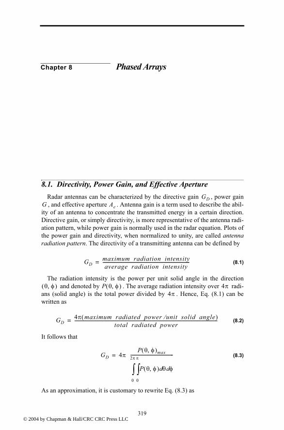
© 200
Chapter 8 Phased Arrays
8.1. Directivity, Power Gain, and Effective Aperture Radar antennas can be characterized by the directive gain , power gain, and effective aperture . Antenna gain is a term used to describe the abil-
ity of an antenna to concentrate the transmitted energy in a certain direction.Directive gain, or simply directivity, is more representative of the antenna radi-ation pattern, while power gain is normally used in the radar equation. Plots ofthe power gain and directivity, when normalized to unity, are called antennaradiation pattern. The directivity of a transmitting antenna can be defined by
(8.1)
The radiation intensity is the power per unit solid angle in the direction and denoted by . The average radiation intensity over radi-
ans (solid angle) is the total power divided by . Hence, Eq. (8.1) can bewritten as
(8.2)
It follows that
(8.3)
As an approximation, it is customary to rewrite Eq. (8.3) as
GDG Ae
GDmaximum radiation intensityaverage radiation intensity
---------------------------------------------------------------------------------=
θ φ,( ) P θ φ,( ) 4π4π
GD4π maximum radiated power unit solid angle⁄( )
total radiated power-------------------------------------------------------------------------------------------------------------------------------------=
GD 4πP θ φ,( )max
P θ φ,( ) θd φd
0
π
∫0
2π
∫----------------------------------------=
3194 by Chapman & Hall/CRC CRC Press LLC
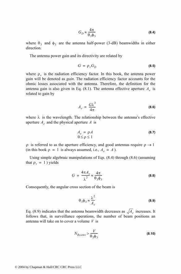
© 200
(8.4)
where and are the antenna half-power (3-dB) beamwidths in eitherdirection.
The antenna power gain and its directivity are related by
(8.5)
where is the radiation efficiency factor. In this book, the antenna powergain will be denoted as gain. The radiation efficiency factor accounts for theohmic losses associated with the antenna. Therefore, the definition for theantenna gain is also given in Eq. (8.1). The antenna effective aperture isrelated to gain by
(8.6)
where is the wavelength. The relationship between the antennas effectiveaperture and the physical aperture is
(8.7)
is referred to as the aperture efficiency, and good antennas require (in this book is always assumed, i.e., ).
Using simple algebraic manipulations of Eqs. (8.4) through (8.6) (assumingthat ) yields
(8.8)
Consequently, the angular cross section of the beam is
(8.9)
Eq. (8.9) indicates that the antenna beamwidth decreases as increases. Itfollows that, in surveillance operations, the number of beam positions anantenna will take on to cover a volume is
(8.10)
GD4πθ3φ3-----------≈
θ3 φ3
G ρrGD=
ρr
Ae
AeGλ2
4π----------=
λAe A
Ae ρA0 ρ 1≤ ≤
=
ρ ρ 1→ρ 1= Ae A=
ρr 1=
G4πAe
λ2------------ 4π
θ3φ3-----------≈=
θ3φ3λ2
Ae-----≈
Ae
V
NBeamsV
θ3φ3----------->
4 by Chapman & Hall/CRC CRC Press LLC
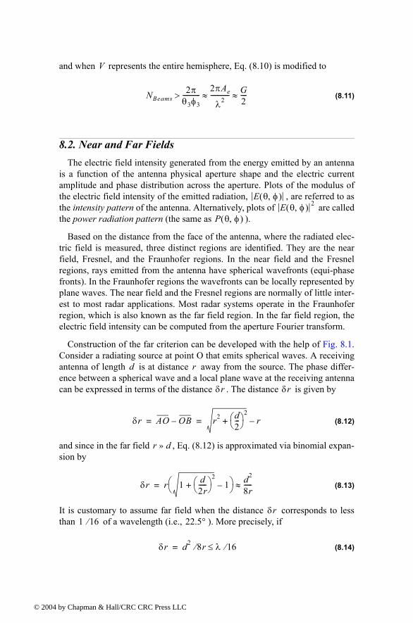
© 200
and when represents the entire hemisphere, Eq. (8.10) is modified to
(8.11)
8.2. Near and Far FieldsThe electric field intensity generated from the energy emitted by an antenna
is a function of the antenna physical aperture shape and the electric currentamplitude and phase distribution across the aperture. Plots of the modulus ofthe electric field intensity of the emitted radiation, , are referred to asthe intensity pattern of the antenna. Alternatively, plots of are calledthe power radiation pattern (the same as ).
Based on the distance from the face of the antenna, where the radiated elec-tric field is measured, three distinct regions are identified. They are the nearfield, Fresnel, and the Fraunhofer regions. In the near field and the Fresnelregions, rays emitted from the antenna have spherical wavefronts (equi-phasefronts). In the Fraunhofer regions the wavefronts can be locally represented byplane waves. The near field and the Fresnel regions are normally of little inter-est to most radar applications. Most radar systems operate in the Fraunhoferregion, which is also known as the far field region. In the far field region, theelectric field intensity can be computed from the aperture Fourier transform.
Construction of the far criterion can be developed with the help of Fig. 8.1.Consider a radiating source at point O that emits spherical waves. A receivingantenna of length is at distance away from the source. The phase differ-ence between a spherical wave and a local plane wave at the receiving antennacan be expressed in terms of the distance . The distance is given by
(8.12)
and since in the far field , Eq. (8.12) is approximated via binomial expan-sion by
(8.13)
It is customary to assume far field when the distance corresponds to lessthan of a wavelength (i.e., ). More precisely, if
(8.14)
V
NBeams2πθ3φ3-----------
2πAe
λ2------------ G
2----≈ ≈>
E θ φ,( )E θ φ,( ) 2
P θ φ,( )
d r
δr δr
δr AO OB r2 d2---
2+ r= =
r d»
δr r 1 d2r-----
2+ 1
d2
8r-----≈=
δr1 16⁄ 22.5°
δr d2 8r⁄ λ 16⁄≤=
4 by Chapman & Hall/CRC CRC Press LLC
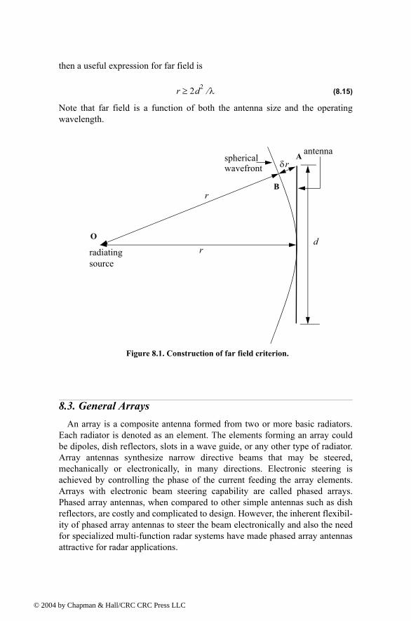
© 200
then a useful expression for far field is
(8.15)
Note that far field is a function of both the antenna size and the operatingwavelength.
8.3. General ArraysAn array is a composite antenna formed from two or more basic radiators.
Each radiator is denoted as an element. The elements forming an array couldbe dipoles, dish reflectors, slots in a wave guide, or any other type of radiator.Array antennas synthesize narrow directive beams that may be steered,mechanically or electronically, in many directions. Electronic steering isachieved by controlling the phase of the current feeding the array elements.Arrays with electronic beam steering capability are called phased arrays.Phased array antennas, when compared to other simple antennas such as dishreflectors, are costly and complicated to design. However, the inherent flexibil-ity of phased array antennas to steer the beam electronically and also the needfor specialized multi-function radar systems have made phased array antennasattractive for radar applications.
r 2d2 λ⁄≥
r
δr
d
r
antennasphericalwavefront
Figure 8.1. Construction of far field criterion.
radiatingsource
O
B
A
4 by Chapman & Hall/CRC CRC Press LLC
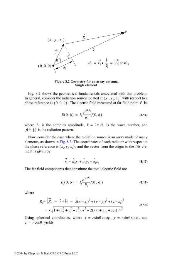
© 200
Fig. 8.2 shows the geometrical fundamentals associated with this problem.In general, consider the radiation source located at with respect to aphase reference at . The electric field measured at far field point is
(8.16)
where is the complex amplitude, is the wave number, andis the radiation pattern.
Now, consider the case where the radiation source is an array made of manyelements, as shown in Fig. 8.3. The coordinates of each radiator with respect tothe phase reference is , and the vector from the origin to the ele-ment is given by
(8.17)
The far field components that constitute the total electric field are
(8.18)
where
(8.19)
Using spherical coordinates, where , , and yields
0 0 0, ,( )θ1
x1 y1 z1, ,( )R1
rr1
p
d1
d1 r1rr-----• r1 θ1cos= =
Figure 8.2 Geometry for an array antenna. Single element
x1 y1 z1, ,( )0 0 0, ,( ) P
E θ φ,( ) I0e
jkR1
R1-------------f θ φ,( )=
I0 k 2π λ⁄=f θ φ,( )
xi yi zi, ,( ) ith
ri ax= xi ay
yi az zi+ +
Ei θ φ,( ) Iie
jkRi
Ri------------f θi φi,( )=
Ri Ri= r ri x xi( )2 y yi( )2 z zi( )2+ += =
r 1 xi2 yi
2 zi2+ +( ) r2⁄ 2 xxi yyi zzi+ +( ) r2⁄+=
x r θ ϕcossin= y r θ ϕsinsin=z r θcos=
4 by Chapman & Hall/CRC CRC Press LLC

© 200
(8.20)
Thus, a good approximation (using binomial expansion) for Eq. (8.19) is
(8.21)
It follows that the phase contribution at the far field point from the radiatorwith respect to the phase reference is
(8.22)
Remember, however, that the unit vector along the vector is
(8.23)
Hence, we can rewrite Eq. (8.22) as
(8.24)
Finally, by virtue of superposition, the total electric field is
(8.25)
which is known as the array factor for an array antenna where the complex cur-rent for the element is .
0 0 0, ,( )
x1 y1 z1, ,( )
xi yi zi, ,( )Ri r ri=
rri
p
ax
θ
r1
R1 r r1=
ay
az
az
az
θ1
Figure 8.3 Geometry for an array antenna.
ax ay
ay
ax
xi2 yi
2 zi2+ +( )
r2-------------------------------- ri
r2------ 1«=
Ri r r xi θ φcossin yi θ φsinsin zi θcos+ +( )=
ith
ejkRi
e jkr ejk xi θ φcossin yi θ φsinsin zi θcos+ +( )
=
r0 r
r0rr----- a x θ φcossin a y θ φsinsin a z θcos+ += =
ejkRi
e jkr ejk ri r0•( ) e jkr ejΨi θ φ,( )
= =
E θ φ,( ) IiejΨi θ φ,( )
i 1=
N
∑=
ith Ii
4 by Chapman & Hall/CRC CRC Press LLC
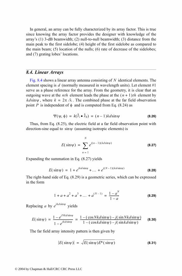
© 200
In general, an array can be fully characterized by its array factor. This is truesince knowing the array factor provides the designer with knowledge of thearrays (1) 3-dB beamwidth; (2) null-to-null beamwidth; (3) distance from themain peak to the first sidelobe; (4) height of the first sidelobe as compared tothe main beam; (5) location of the nulls; (6) rate of decrease of the sidelobes;and (7) grating lobes locations.
8.4. Linear ArraysFig. 8.4 shows a linear array antenna consisting of identical elements. The
element spacing is (normally measured in wavelength units). Let element #1serve as a phase reference for the array. From the geometry, it is clear that anoutgoing wave at the element leads the phase at the element by
, where . The combined phase at the far field observationpoint is independent of and is computed from Eq. (8.24) as
(8.26)
Thus, from Eq. (8.25), the electric field at a far field observation point withdirection-sine equal to (assuming isotropic elements) is
(8.27)
Expanding the summation in Eq. (8.27) yields
(8.28)
The right-hand side of Eq. (8.29) is a geometric series, which can be expressedin the form
(8.29)
Replacing by yields
(8.30)
The far field array intensity pattern is then given by
(8.31)
Nd
nth n 1+( )thkd ψsin k 2π λ⁄=
P φ
Ψ ψ φ,( ) k ri r0•( ) n 1( )kd ψsin= =
ψsin
E ψsin( ) ej n 1( ) kd ψsin( )
n 1=
N
∑=
E ψsin( ) 1 ejkd ψsin … ej N 1( ) kd ψsin( )+ + +=
1 a a2 a3 … a N 1( )+ + + + + 1 aN1 a
---------------=
a ejkd ψsin
E ψsin( ) 1 ejNkd ψsin
1 ejkd ψsin----------------------------- 1 Nkd ψsincos( ) j Nkd ψsinsin( )
1 kd ψsincos( ) j kd ψsinsin( )-----------------------------------------------------------------------------------------= =
E ψsin( ) E ψsin( )E∗ ψsin( )=
4 by Chapman & Hall/CRC CRC Press LLC
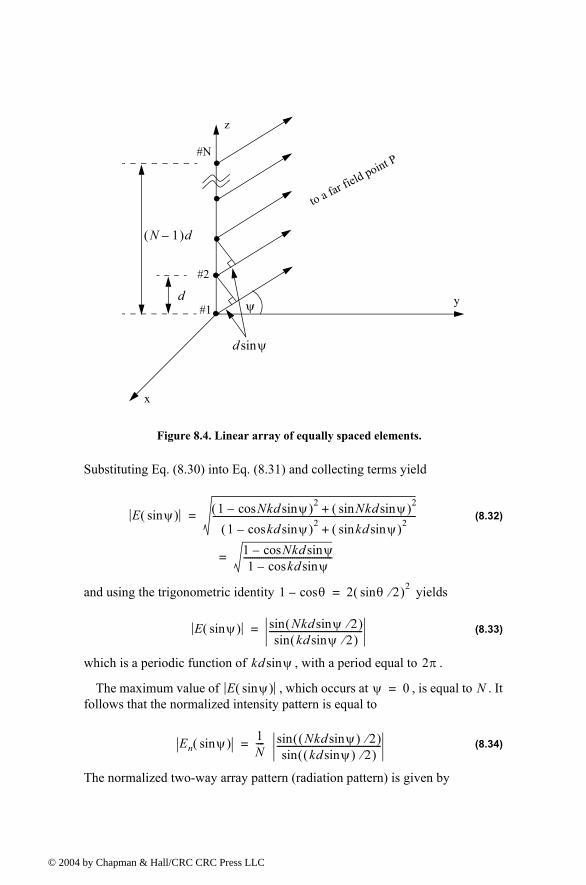
© 200
Substituting Eq. (8.30) into Eq. (8.31) and collecting terms yield
(8.32)
and using the trigonometric identity yields
(8.33)
which is a periodic function of , with a period equal to .
The maximum value of , which occurs at , is equal to . Itfollows that the normalized intensity pattern is equal to
(8.34)
The normalized two-way array pattern (radiation pattern) is given by
y
z
x
to a far field point P
ψ
d ψsin
d
N 1( )d
Figure 8.4. Linear array of equally spaced elements.
#1
#2
#N
E ψsin( ) 1 Nkd ψsincos( )2 Nkd ψsinsin( )2+
1 kd ψsincos( )2 kd ψsinsin( )2+--------------------------------------------------------------------------------------------
1 Nkd ψsincos1 kd ψsincos
----------------------------------------
=
=
1 θcos 2 θ 2⁄sin( )2=
E ψsin( ) Nkd ψsin 2⁄( )sinkd ψsin 2⁄( )sin
------------------------------------------=
kd ψsin 2π
E ψsin( ) ψ 0= N
En ψsin( ) 1N---- Nkd ψsin( ) 2⁄( )sin
kd ψsin( ) 2⁄( )sin-----------------------------------------------=
4 by Chapman & Hall/CRC CRC Press LLC
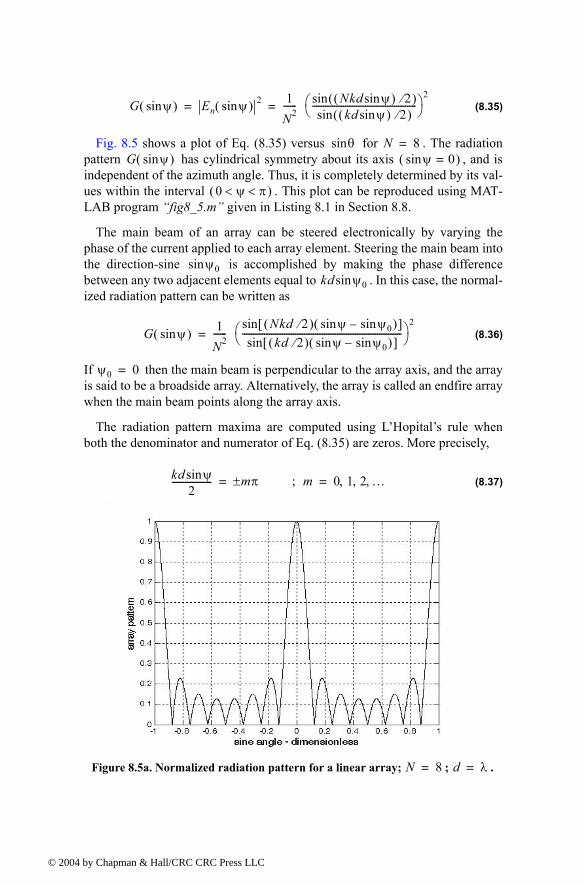
© 200
(8.35)
Fig. 8.5 shows a plot of Eq. (8.35) versus for . The radiationpattern has cylindrical symmetry about its axis , and isindependent of the azimuth angle. Thus, it is completely determined by its val-ues within the interval . This plot can be reproduced using MAT-LAB program fig8_5.m given in Listing 8.1 in Section 8.8.
The main beam of an array can be steered electronically by varying thephase of the current applied to each array element. Steering the main beam intothe direction-sine is accomplished by making the phase differencebetween any two adjacent elements equal to . In this case, the normal-ized radiation pattern can be written as
(8.36)
If then the main beam is perpendicular to the array axis, and the arrayis said to be a broadside array. Alternatively, the array is called an endfire arraywhen the main beam points along the array axis.
The radiation pattern maxima are computed using LHopitals rule whenboth the denominator and numerator of Eq. (8.35) are zeros. More precisely,
(8.37)
G ψsin( ) En ψsin( ) 2 1N2------ Nkd ψsin( ) 2⁄( )sin
kd ψsin( ) 2⁄( )sin-----------------------------------------------
2= =
θsin N 8=G ψsin( ) ψsin 0=( )
0 ψ π< <( )
ψ0sinkd ψ0sin
G ψsin( ) 1N2------
Nkd 2⁄( ) ψsin ψ0sin( )[ ]sinkd 2⁄( ) ψsin ψ0sin( )[ ]sin
------------------------------------------------------------------------
2=
ψ0 0=
kd ψsin2
------------------ mπ±= m; 0 1 2 …, , ,=
Figure 8.5a. Normalized radiation pattern for a linear array; ; .N 8= d λ=
4 by Chapman & Hall/CRC CRC Press LLC
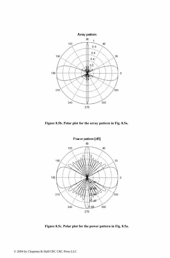
© 200
Figure 8.5b. Polar plot for the array pattern in Fig. 8.5a.
Figure 8.5c. Polar plot for the power pattern in Fig. 8.5a.
4 by Chapman & Hall/CRC CRC Press LLC
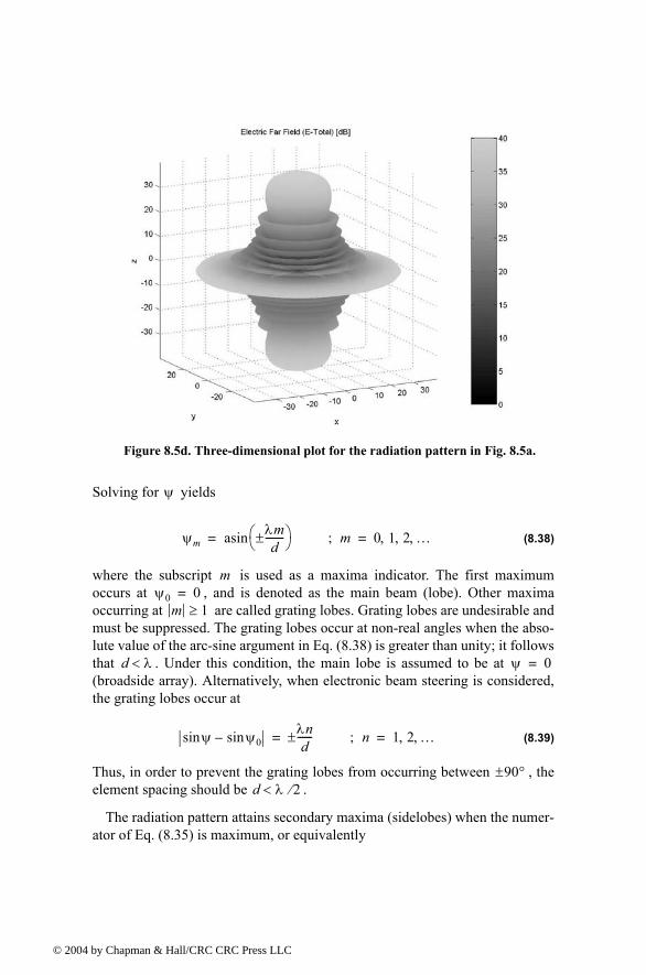
© 200
Solving for yields
(8.38)
where the subscript is used as a maxima indicator. The first maximumoccurs at , and is denoted as the main beam (lobe). Other maximaoccurring at are called grating lobes. Grating lobes are undesirable andmust be suppressed. The grating lobes occur at non-real angles when the abso-lute value of the arc-sine argument in Eq. (8.38) is greater than unity; it followsthat . Under this condition, the main lobe is assumed to be at (broadside array). Alternatively, when electronic beam steering is considered,the grating lobes occur at
(8.39)
Thus, in order to prevent the grating lobes from occurring between , theelement spacing should be .
The radiation pattern attains secondary maxima (sidelobes) when the numer-ator of Eq. (8.35) is maximum, or equivalently
Figure 8.5d. Three-dimensional plot for the radiation pattern in Fig. 8.5a.
ψ
ψmλmd
-------± asin= ; m 0 1 2 …, , ,=
mψ0 0=
m 1≥
d λ< ψ 0=
ψsin ψ0sinλnd
------±= n; 1 2 …, ,=
90°±d λ 2⁄<
4 by Chapman & Hall/CRC CRC Press LLC
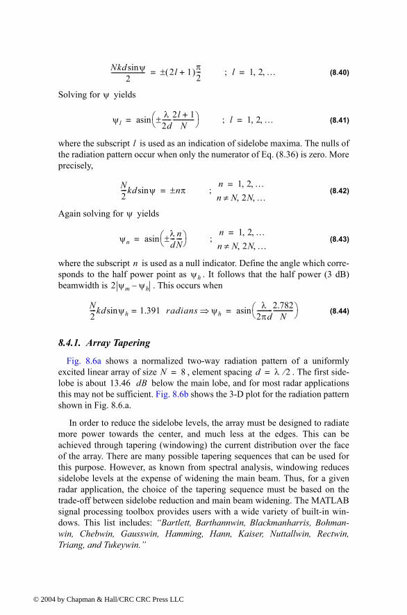
© 200
(8.40)
Solving for yields
(8.41)
where the subscript is used as an indication of sidelobe maxima. The nulls ofthe radiation pattern occur when only the numerator of Eq. (8.36) is zero. Moreprecisely,
(8.42)
Again solving for yields
(8.43)
where the subscript is used as a null indicator. Define the angle which corre-sponds to the half power point as . It follows that the half power (3 dB)beamwidth is . This occurs when
(8.44)
8.4.1. Array Tapering
Fig. 8.6a shows a normalized two-way radiation pattern of a uniformlyexcited linear array of size , element spacing . The first side-lobe is about below the main lobe, and for most radar applicationsthis may not be sufficient. Fig. 8.6b shows the 3-D plot for the radiation patternshown in Fig. 8.6.a.
In order to reduce the sidelobe levels, the array must be designed to radiatemore power towards the center, and much less at the edges. This can beachieved through tapering (windowing) the current distribution over the faceof the array. There are many possible tapering sequences that can be used forthis purpose. However, as known from spectral analysis, windowing reducessidelobe levels at the expense of widening the main beam. Thus, for a givenradar application, the choice of the tapering sequence must be based on thetrade-off between sidelobe reduction and main beam widening. The MATLABsignal processing toolbox provides users with a wide variety of built-in win-dows. This list includes: Bartlett, Barthannwin, Blackmanharris, Bohman-win, Chebwin, Gausswin, Hamming, Hann, Kaiser, Nuttallwin, Rectwin,Triang, and Tukeywin.
Nkd ψsin2
---------------------- 2l 1+( )π2---±= l; 1 2 …, ,=
ψ
ψlλ
2d------2l 1+
N--------------±
asin= l; 1 2 …, ,=
l
N2----kd ψsin nπ±= ;
n 1 2 …, ,=
n N 2N …,,≠
ψ
ψnλd---± n
N----
asin=n 1 2 …, ,=
n N 2N …,,≠;
nψh
2 ψm ψh
N2----kd ψhsin 1.391= radians ψh⇒ λ
2πd----------2.782
N-------------
asin=
N 8= d λ 2⁄=13.46 dB
4 by Chapman & Hall/CRC CRC Press LLC
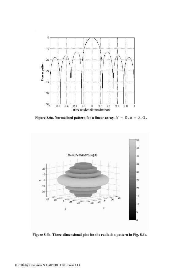
© 200
Figure 8.6a. Normalized pattern for a linear array. , .N 8= d λ 2⁄=
Figure 8.6b. Three-dimensional plot for the radiation pattern in Fig. 8.6a.
4 by Chapman & Hall/CRC CRC Press LLC
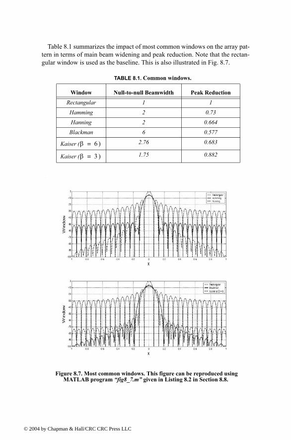
© 200
Table 8.1 summarizes the impact of most common windows on the array pat-tern in terms of main beam widening and peak reduction. Note that the rectan-gular window is used as the baseline. This is also illustrated in Fig. 8.7.
TABLE 8.1. Common windows.
Window Null-to-null Beamwidth Peak Reduction
Rectangular 1 1
Hamming 2 0.73
Hanning 2 0.664
Blackman 6 0.577
Kaiser ( 2.76 0.683
Kaiser ( 1.75 0.882
β 6 )=
β 3 )=
Figure 8.7. Most common windows. This figure can be reproduced using MATLAB program fig8_7.m given in Listing 8.2 in Section 8.8.
4 by Chapman & Hall/CRC CRC Press LLC
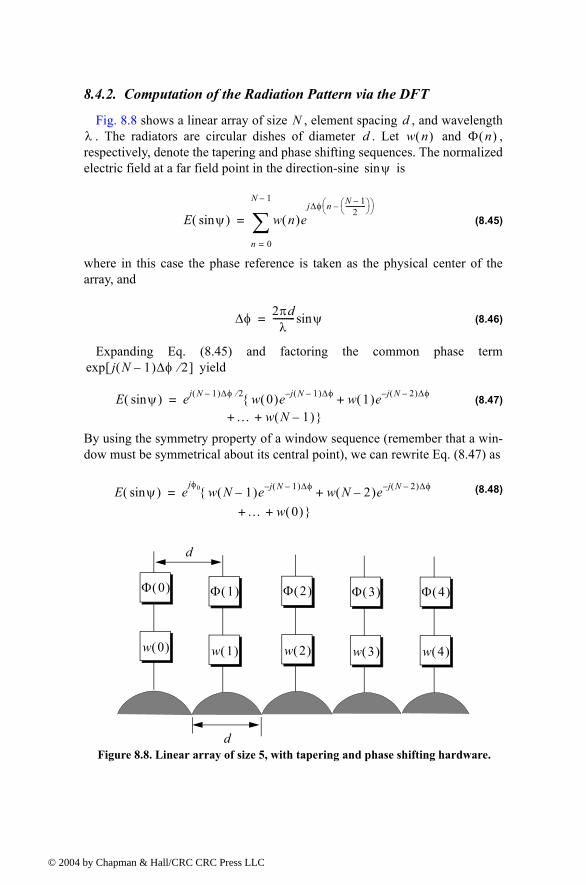
© 200
8.4.2. Computation of the Radiation Pattern via the DFT
Fig. 8.8 shows a linear array of size , element spacing , and wavelength. The radiators are circular dishes of diameter . Let and ,
respectively, denote the tapering and phase shifting sequences. The normalizedelectric field at a far field point in the direction-sine is
(8.45)
where in this case the phase reference is taken as the physical center of thearray, and
(8.46)
Expanding Eq. (8.45) and factoring the common phase term yield
(8.47)
By using the symmetry property of a window sequence (remember that a win-dow must be symmetrical about its central point), we can rewrite Eq. (8.47) as
(8.48)
N dλ d w n( ) Φ n( )
ψsin
E ψsin( ) w n( )ej∆φ n N 1
2-------------
n 0=
N 1
∑=
∆φ 2πdλ
---------- ψsin=
j N 1( )∆φ 2⁄[ ]exp
E ψsin( ) ej N 1( )∆φ 2⁄ w 0( )e j N 1( )∆φ w 1( )e j N 2( )∆φ
… w N 1( )+
+ +
=
E ψsin( ) ejφ0 w N 1( )e j N 1( )∆φ w N 2( )e j N 2( )∆φ
… w 0( )+
+ +
=
w 0( )
Φ 0( )
w 1( )
Φ 1( )
w 3( )
Φ 3( )
w 4( )
Φ 4( )
w 2( )
Φ 2( )
d
d Figure 8.8. Linear array of size 5, with tapering and phase shifting hardware.
4 by Chapman & Hall/CRC CRC Press LLC
© 200
where .
Define . It follows that
(8.49)
The discrete Fourier transform of the sequence is defined as
(8.50)
The set which makes equal to the DFT kernel is
(8.51)
Then by using Eq. (8.51) in Eq. (8.50) yields
(8.52)
The one-way array pattern is computed as the modulus of Eq. (8.52). It followsthat the one-way radiation pattern of a tapered linear array of circular dishes is
(8.53)
where is the element pattern.
In practice, phase shifters are normally implemented as part of the Transmit/Receive (TR) modules, using a finite number of bits. Consequently, due to thequantization error (difference between desired phase and actual quantizedphase) the sidelobe levels are affected.
MATLAB Function linear_array.m
The function linear_array.m computes and plots the linear array gain pat-tern as a function of real sine-space (sine the steering angle). It is given in List-ing 8.3 in Section 8.8. The syntax is as follows:
[theta, patternr, patterng] = linear_array(Nr, dolr, theta0, winid, win, nbits)
φ0 N 1( )∆φ 2⁄=
V1n j∆φn( ) n;exp 0 1 … N 1, , ,= =
E ψsin( ) ejφ0 w 0( ) w 1( )V1
1 … w N 1( )V1N 1+ + +[ ]
ejφ0 w n( )V1
n
n 0=
N 1
∑
=
=
w n( )
W q( ) w n( )ej2πnq( )
N--------------------
n 0=
N 1
∑= q; 0 1 … N 1, , ,=
ψqsin V1
ψqsin λqNd-------= q; 0 1 … N 1, , ,=
E ψsin( ) ejφ0W q( )=
G ψsin( ) Ge W q( )=
Ge
4 by Chapman & Hall/CRC CRC Press LLC
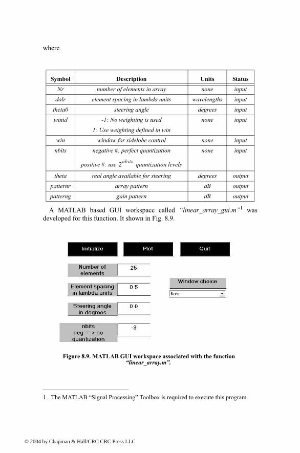
© 200
where
A MATLAB based GUI workspace called linear_array_gui.m1 wasdeveloped for this function. It shown in Fig. 8.9.
Symbol Description Units Status
Nr number of elements in array none input
dolr element spacing in lambda units wavelengths input
theta0 steering angle degrees input
winid -1: No weighting is used
1: Use weighting defined in win
none input
win window for sidelobe control none input
nbits negative #: perfect quantization
positive #: use quantization levels
none input
theta real angle available for steering degrees output
patternr array pattern dB output
patterng gain pattern dB output
1. The MATLAB Signal Processing Toolbox is required to execute this program.
2nbits
Figure 8.9. MATLAB GUI workspace associated with the function linear_array.m.
4 by Chapman & Hall/CRC CRC Press LLC
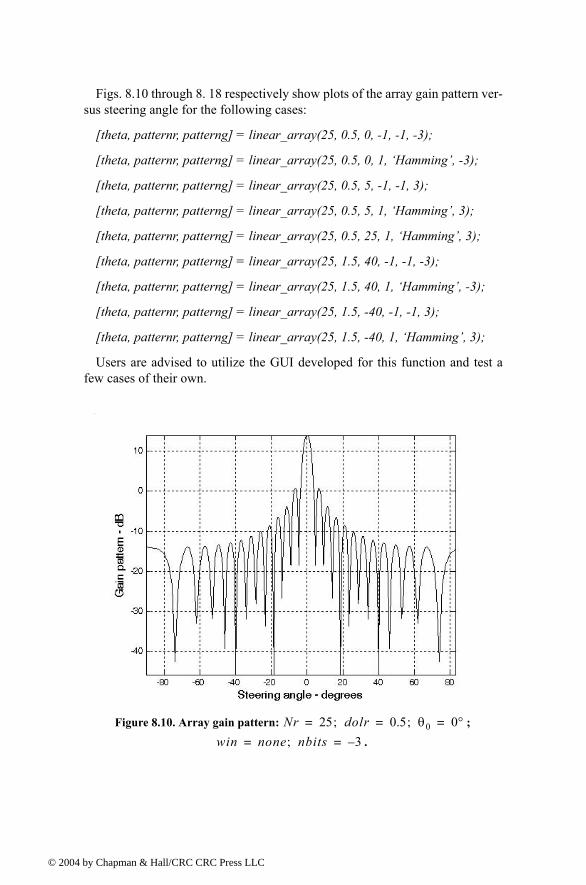
© 200
Figs. 8.10 through 8. 18 respectively show plots of the array gain pattern ver-sus steering angle for the following cases:
[theta, patternr, patterng] = linear_array(25, 0.5, 0, -1, -1, -3);
[theta, patternr, patterng] = linear_array(25, 0.5, 0, 1, Hamming, -3);
[theta, patternr, patterng] = linear_array(25, 0.5, 5, -1, -1, 3);
[theta, patternr, patterng] = linear_array(25, 0.5, 5, 1, Hamming, 3);
[theta, patternr, patterng] = linear_array(25, 0.5, 25, 1, Hamming, 3);
[theta, patternr, patterng] = linear_array(25, 1.5, 40, -1, -1, -3);
[theta, patternr, patterng] = linear_array(25, 1.5, 40, 1, Hamming, -3);
[theta, patternr, patterng] = linear_array(25, 1.5, -40, -1, -1, 3);
[theta, patternr, patterng] = linear_array(25, 1.5, -40, 1, Hamming, 3);
Users are advised to utilize the GUI developed for this function and test afew cases of their own.
Figure 8.10. Array gain pattern: ;
.
Nr 25 dolr; 0.5 θ0; 0°= = =
win none nbits; 3= =
4 by Chapman & Hall/CRC CRC Press LLC
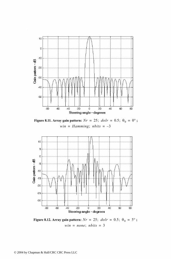
© 200
Figure 8.11. Array gain pattern: ; Nr 25 dolr; 0.5 θ0; 0°= = =
win Hamming nbits; 3= =
Figure 8.12. Array gain pattern: ; Nr 25 dolr; 0.5 θ0; 5°= = =
win none nbits; 3= =
4 by Chapman & Hall/CRC CRC Press LLC
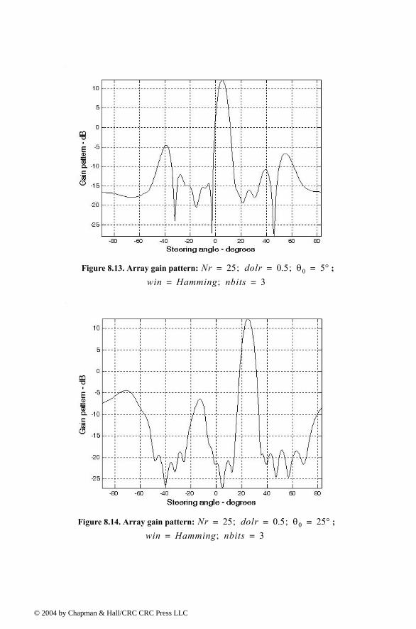
© 200
Figure 8.13. Array gain pattern: ; Nr 25 dolr; 0.5 θ0; 5°= = =
win Hamming nbits; 3= =
Figure 8.14. Array gain pattern: ; Nr 25 dolr; 0.5 θ0; 25°= = =
win Hamming nbits; 3= =
4 by Chapman & Hall/CRC CRC Press LLC
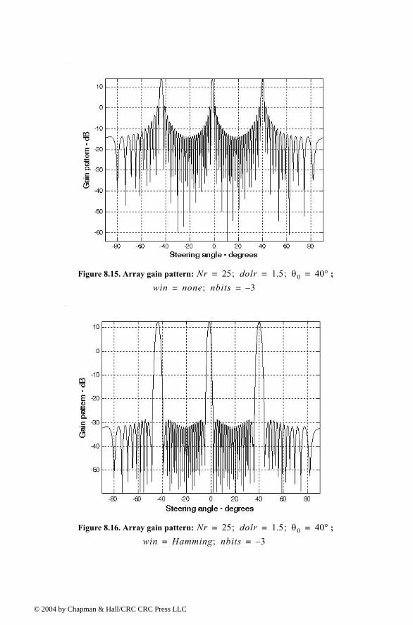
© 200
Figure 8.15. Array gain pattern: ; Nr 25 dolr; 1.5 θ0; 40°= = =
win none nbits; 3= =
Figure 8.16. Array gain pattern: ; Nr 25 dolr; 1.5 θ0; 40°= = =
win Hamming nbits; 3= =
4 by Chapman & Hall/CRC CRC Press LLC
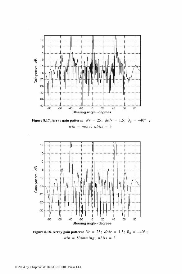
© 200
Figure 8.17. Array gain pattern: ; Nr 25 dolr; 1.5 θ0; 40 °= = =
win none nbits; 3= =
Figure 8.18. Array gain pattern: ; Nr 25 dolr; 1.5 θ0; 40 °= = =
win Hamming nbits; 3= =
4 by Chapman & Hall/CRC CRC Press LLC
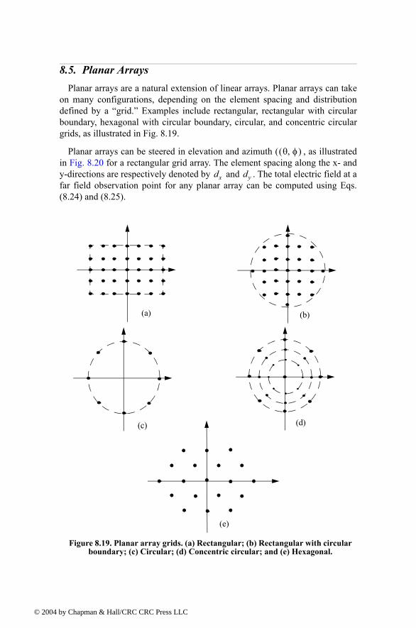
© 200
8.5. Planar ArraysPlanar arrays are a natural extension of linear arrays. Planar arrays can take
on many configurations, depending on the element spacing and distributiondefined by a grid. Examples include rectangular, rectangular with circularboundary, hexagonal with circular boundary, circular, and concentric circulargrids, as illustrated in Fig. 8.19.
Planar arrays can be steered in elevation and azimuth ( , as illustratedin Fig. 8.20 for a rectangular grid array. The element spacing along the x- andy-directions are respectively denoted by and . The total electric field at afar field observation point for any planar array can be computed using Eqs.(8.24) and (8.25).
θ φ,( )
dx dy
(a) (b)
(c) (d)
(e)
Figure 8.19. Planar array grids. (a) Rectangular; (b) Rectangular with circular boundary; (c) Circular; (d) Concentric circular; and (e) Hexagonal.
4 by Chapman & Hall/CRC CRC Press LLC
© 200
Rectangular Grid Arrays
Consider the rectangular grid as shown in Fig. 8.20. The dot product, where the vector is the vector to the element in the array and
is the unit vector to the far field observation point, can be broken linearly intoits x- and y-components. It follows that the electric field components due to theelements distributed along the x- and y-directions are respectively, given by
(8.54)
(8.55)
The total electric field at the far field observation point is then given by
(8.56)
N M×ri r0• ri ith r0
y
z
x
φθ
dy
dx
far field point
Figure 8.20. Rectangular array geometry.
Ex θ φ,( ) Ixne
j n 1( )kdx θ φcossin
n 1=
N
∑=
Ey θ φ,( ) Iyme
j m 1( )kdy θ φsinsin
m 1=
N
∑=
E θ φ,( ) Ex θ φ,( )Ey θ φ,( )
Iyme
j m 1( )kdy θ φsinsin
m 1=
N
∑
Ixne
j n 1( )kdx θ φcossin
n 1=
N
∑
= =
4 by Chapman & Hall/CRC CRC Press LLC
© 200
Eq. (8.56) can be expressed in terms of the directional cosines
(8.57a)
(8.57b)
The visible region is then defined by
(8.58)
It is very common to express a planar arrays ability to steer the beam inspace in terms of the space instead of the angles . Fig. 8.21 showshow a beam steered in a certain direction is translated into space.
u θ φcossin=
v θ φsinsin=
φ uv--- atan=
θ u2 v2+asin=
u2 v2+ 1≤
U V, θ φ,θ φ, U V,
θ
φ
V
U
Figure 8.21. Translation from spherical coordinates into U,V space.
1
4 by Chapman & Hall/CRC CRC Press LLC
© 200
The rectangular array one-way intensity pattern is then equal to the productof the individual patterns. More precisely for a uniform excitation( ),
(8.59)
The radiation pattern maxima, nulls, sidelobes, and grating lobes in both thex- and y-axes are computed in a similar fashion to the linear array case. Addi-tionally, the same conditions for grating lobe control are applicable. Note thesymmetry is about the angle .
Circular Grid Arrays
The geometry of interest is shown in Fig. 8.19c. In this case, elements aredistributed equally on the outer circle whose radius is . For this purpose con-sider the geometry shown in Fig. 8.22. From the geometry
(8.60)
The coordinates of the element are
(8.61)
It follows that
(8.62)
which can be rearranged as
(8.63)
Then by using the identity , Eq.(8.63)collapses to
(8.64)
Finally by using Eq. (8.25), the far field electric field is then given by
(8.65)
IymIxn
const= =
E θ φ,( ) Nkdx θ φcossin( ) 2⁄( )sinkdx θ φcossin( ) 2⁄( )sin
-------------------------------------------------------------Nkdy θ φsinsin( ) 2⁄( )sinkdy θ φsinsin( ) 2⁄( )sin
------------------------------------------------------------=
φ
Na
Φn2πN------ n= n; 1 2 … N, , ,=
nth
xn a Φncos=
yn a Φnsin=
zn 0=
k rn r0•( ) Ψn k a θ φ Φncoscossin a θ φ Φnsinsinsin 0+ +( )= =
Ψn ak θ φ Φncoscos φ Φnsinsin+( )sin=
A B( )cos A Bcoscos A Bsinsin+=
Ψn ak θ Φn φ( )cossin=
E θ φ a;,( ) In j2πaλ
---------- θ Φn φ( )cossin
exp
n 1=
N
∑=
4 by Chapman & Hall/CRC CRC Press LLC
© 200
where represents the complex current distribution for the element.When the array main beam is directed in the , Eq. (8.65) takes on thefollowing form
(8.66)
MATLAB program circular_array.m
The MATLAB program circular_array.m calculates and plots the rectan-gular and polar array patterns for a circular array versus and constantplanes. It is given in Listing 8.4 in Section 8.8. The input parameters to thisprogram include:
Symbol Description Units
a Circular array radius
N number of elements none
theta0 main direction in degrees
phi0 main direction in degrees
Variations Theta; or Phi none
In nthθ0 φ0,( )
E θ φ a;,( ) In j2πaλ
---------- θ Φn φ( )cossin θ0 Φn φ0( )cossin[ ]
exp
n 1=
N
∑=
x
y
z
Φ1
θ
φ
N
N 1
12
P
θ
a
Figure 8.22. Geometry for a circular array.
N 2
θ φ
λ
θ
φ
4 by Chapman & Hall/CRC CRC Press LLC
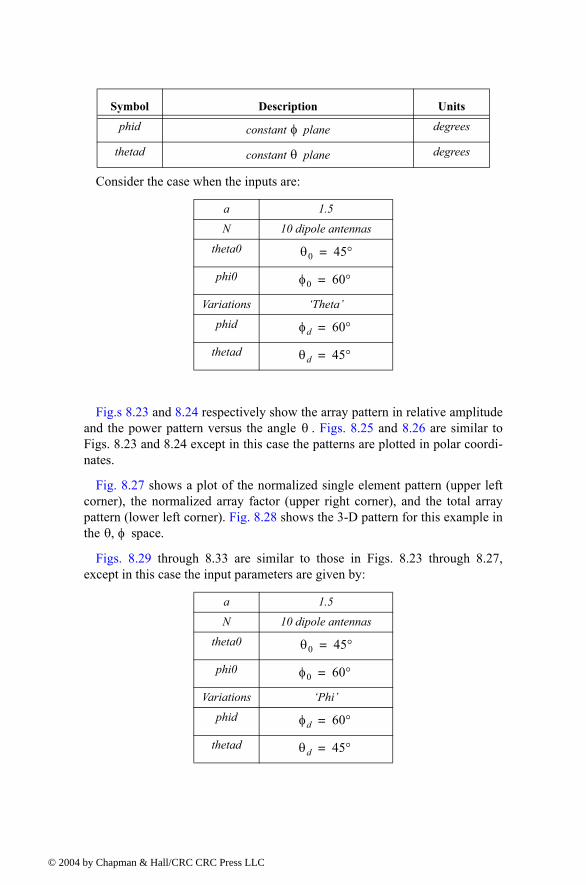
© 200
Consider the case when the inputs are:
Fig.s 8.23 and 8.24 respectively show the array pattern in relative amplitudeand the power pattern versus the angle . Figs. 8.25 and 8.26 are similar toFigs. 8.23 and 8.24 except in this case the patterns are plotted in polar coordi-nates.
Fig. 8.27 shows a plot of the normalized single element pattern (upper leftcorner), the normalized array factor (upper right corner), and the total arraypattern (lower left corner). Fig. 8.28 shows the 3-D pattern for this example inthe space.
Figs. 8.29 through 8.33 are similar to those in Figs. 8.23 through 8.27,except in this case the input parameters are given by:
phid constant plane degrees
thetad constant plane degrees
a 1.5
N 10 dipole antennas
theta0
phi0
Variations Theta
phid
thetad
a 1.5
N 10 dipole antennas
theta0
phi0
Variations Phi
phid
thetad
Symbol Description Units
φ
θ
θ0 45°=
φ0 60°=
φd 60°=
θd 45°=
θ
θ φ,
θ0 45°=
φ0 60°=
φd 60°=
θd 45°=
4 by Chapman & Hall/CRC CRC Press LLC
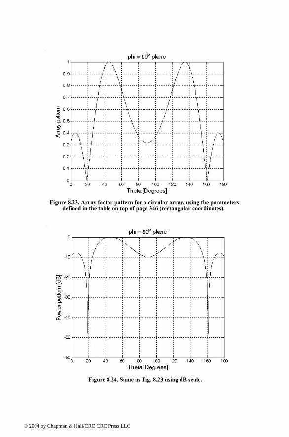
© 200
Figure 8.23. Array factor pattern for a circular array, using the parameters defined in the table on top of page 346 (rectangular coordinates).
Figure 8.24. Same as Fig. 8.23 using dB scale.
4 by Chapman & Hall/CRC CRC Press LLC
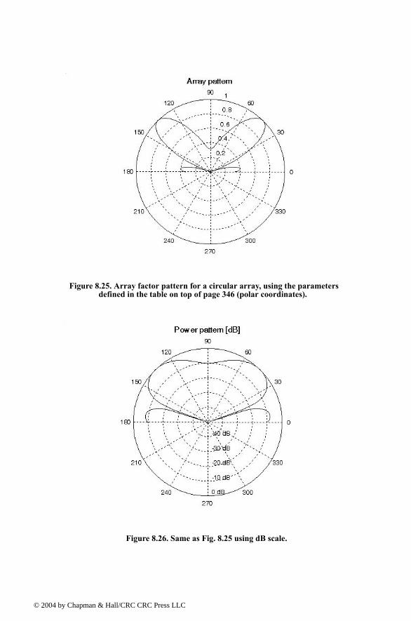
© 200
Figure 8.25. Array factor pattern for a circular array, using the parameters defined in the table on top of page 346 (polar coordinates).
Figure 8.26. Same as Fig. 8.25 using dB scale.
4 by Chapman & Hall/CRC CRC Press LLC
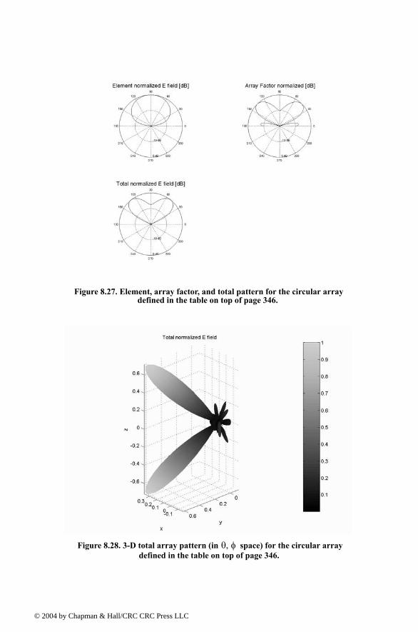
© 200
Figure 8.27. Element, array factor, and total pattern for the circular array defined in the table on top of page 346.
Figure 8.28. 3-D total array pattern (in space) for the circular array defined in the table on top of page 346.
θ φ,
4 by Chapman & Hall/CRC CRC Press LLC
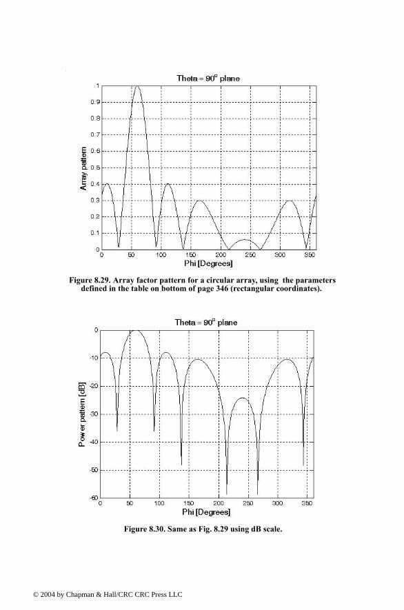
© 200
Figure 8.29. Array factor pattern for a circular array, using the parameters defined in the table on bottom of page 346 (rectangular coordinates).
Figure 8.30. Same as Fig. 8.29 using dB scale.
4 by Chapman & Hall/CRC CRC Press LLC
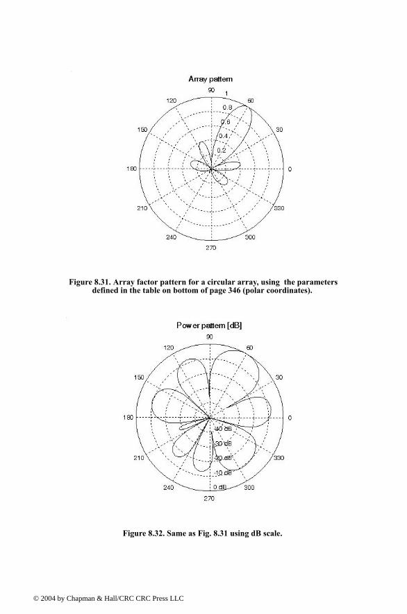
© 200
Figure 8.31. Array factor pattern for a circular array, using the parameters defined in the table on bottom of page 346 (polar coordinates).
Figure 8.32. Same as Fig. 8.31 using dB scale.
4 by Chapman & Hall/CRC CRC Press LLC
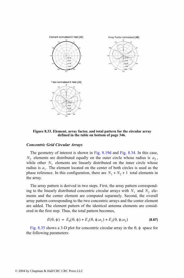
© 200
Concentric Grid Circular Arrays
The geometry of interest is shown in Fig. 8.19d and Fig. 8.34. In this case, elements are distributed equally on the outer circle whose radius is ,
while other elements are linearly distributed on the inner circle whoseradius is . The element located on the center of both circles is used as thephase reference. In this configuration, there are total elements inthe array.
The array pattern is derived in two steps. First, the array pattern correspond-ing to the linearly distributed concentric circular arrays with and ele-ments and the center element are computed separately. Second, the overallarray pattern corresponding to the two concentric arrays and the center elementare added. The element pattern of the identical antenna elements are consid-ered in the first step. Thus, the total pattern becomes,
(8.67)
Fig. 8.35 shows a 3-D plot for concentric circular array in the space forthe following parameters:
Figure 8.33. Element, array factor, and total pattern for the circular array defined in the table on bottom of page 346.
N2 a2N1
a1N1 N2 1+ +
N1 N2
E θ φ,( ) E0 θ φ,( ) E1 θ φ a1;,( ) E2 θ φ a2;,( )+ +=
θ φ,
4 by Chapman & Hall/CRC CRC Press LLC
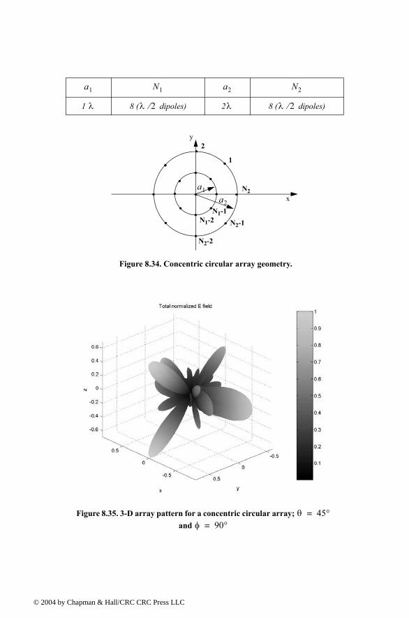
© 200
1 8 ( dipoles) 2 8 ( dipoles)
a1 N1 a2 N2
λ λ 2⁄ λ λ 2⁄
x
y
N2
1
2
N2-1
N2-2
a1a2
Figure 8.34. Concentric circular array geometry.
N1-1N1-2
Figure 8.35. 3-D array pattern for a concentric circular array; and
θ 45°=φ 90°=
4 by Chapman & Hall/CRC CRC Press LLC
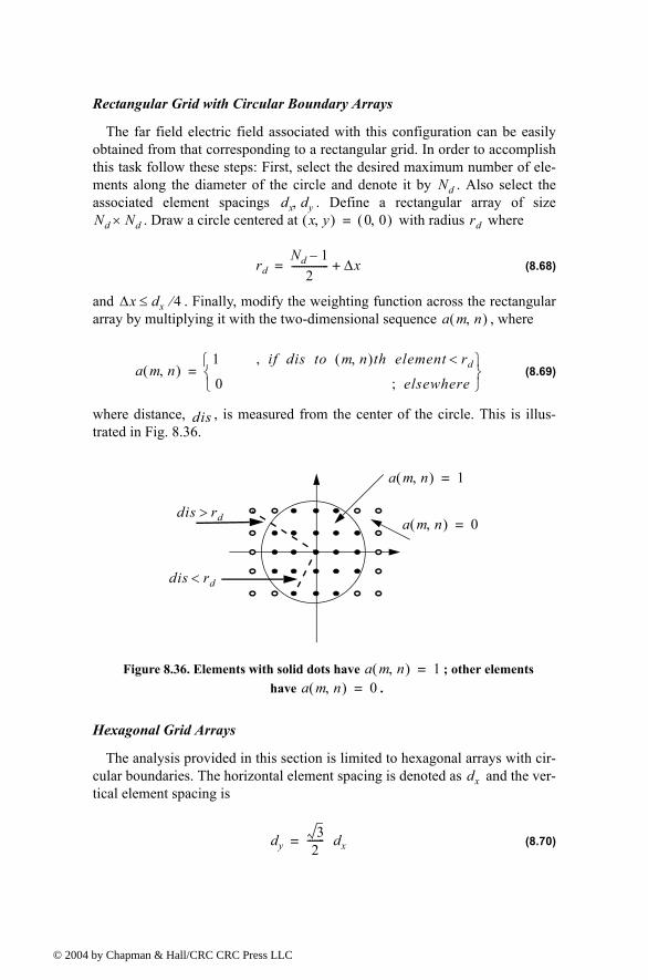
© 200
Rectangular Grid with Circular Boundary Arrays
The far field electric field associated with this configuration can be easilyobtained from that corresponding to a rectangular grid. In order to accomplishthis task follow these steps: First, select the desired maximum number of ele-ments along the diameter of the circle and denote it by . Also select theassociated element spacings . Define a rectangular array of size
. Draw a circle centered at with radius where
(8.68)
and . Finally, modify the weighting function across the rectangulararray by multiplying it with the two-dimensional sequence , where
(8.69)
where distance, , is measured from the center of the circle. This is illus-trated in Fig. 8.36.
Hexagonal Grid Arrays
The analysis provided in this section is limited to hexagonal arrays with cir-cular boundaries. The horizontal element spacing is denoted as and the ver-tical element spacing is
(8.70)
Nddx dy,
Nd Nd× x y,( ) 0 0,( )= rd
rdNd 1
2--------------- ∆x+=
∆x dx 4⁄≤a m n,( )
a m n,( )1 if dis to m n,( )th element rd<,
0 elsewhere;
=
dis
a m n,( ) 1=
a m n,( ) 0=
Figure 8.36. Elements with solid dots have ; other elements have .
a m n,( ) 1=a m n,( ) 0=
dis rd>
dis rd<
dx
dy3
2------- dx=
4 by Chapman & Hall/CRC CRC Press LLC
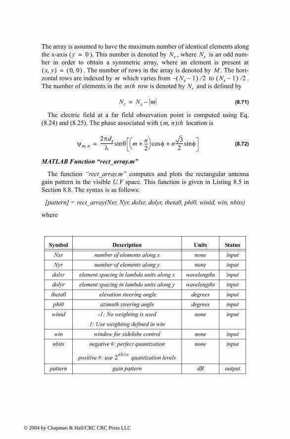
© 200
The array is assumed to have the maximum number of identical elements alongthe x-axis ( ). This number is denoted by , where is an odd num-ber in order to obtain a symmetric array, where an element is present at
. The number of rows in the array is denoted by . The hori-zontal rows are indexed by which varies from to .The number of elements in the row is denoted by and is defined by
(8.71)
The electric field at a far field observation point is computed using Eq.(8.24) and (8.25). The phase associated with location is
(8.72)
MATLAB Function rect_array.m
The function rect_array.m computes and plots the rectangular antennagain pattern in the visible U,V space. This function is given in Listing 8.5 inSection 8.8. The syntax is as follows:
[pattern] = rect_array(Nxr, Nyr, dolxr, dolyr, theta0, phi0, winid, win, nbits)
where
Symbol Description Units Status
Nxr number of elements along x none input
Nyr number of elements along y none input
dolxr element spacing in lambda units along x wavelengths input
dolyr element spacing in lambda units along y wavelengths input
theta0 elevation steering angle degrees input
phi0 azimuth steering angle degrees input
winid -1: No weighting is used
1: Use weighting defined in win
none input
win window for sidelobe control none input
nbits negative #: perfect quantization
positive #: use quantization levels
none input
pattern gain pattern dB output
y 0= Nx Nx
x y,( ) 0 0,( )= Mm Nx 1( ) 2⁄ Nx 1( ) 2⁄
mth Nr
Nr Nx m=
m n,( )th
ψm n,2πdx
λ------------ θ m n
2---+
φcos n 32
------- φsin+sin=
2nbits
4 by Chapman & Hall/CRC CRC Press LLC
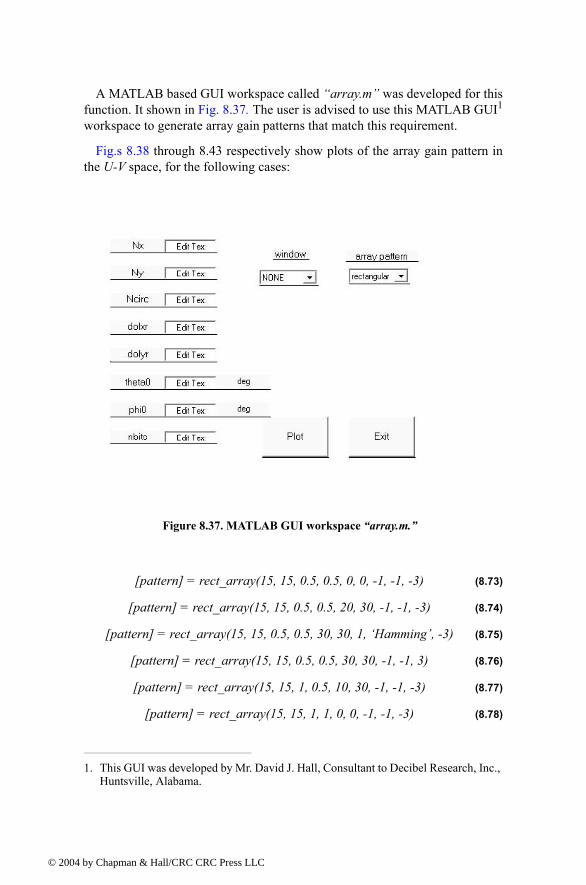
© 200
A MATLAB based GUI workspace called array.m was developed for thisfunction. It shown in Fig. 8.37. The user is advised to use this MATLAB GUI1
workspace to generate array gain patterns that match this requirement.
Fig.s 8.38 through 8.43 respectively show plots of the array gain pattern inthe U-V space, for the following cases:
[pattern] = rect_array(15, 15, 0.5, 0.5, 0, 0, -1, -1, -3) (8.73)
[pattern] = rect_array(15, 15, 0.5, 0.5, 20, 30, -1, -1, -3) (8.74)
[pattern] = rect_array(15, 15, 0.5, 0.5, 30, 30, 1, Hamming, -3) (8.75)
[pattern] = rect_array(15, 15, 0.5, 0.5, 30, 30, -1, -1, 3) (8.76)
[pattern] = rect_array(15, 15, 1, 0.5, 10, 30, -1, -1, -3) (8.77)
[pattern] = rect_array(15, 15, 1, 1, 0, 0, -1, -1, -3) (8.78)
1. This GUI was developed by Mr. David J. Hall, Consultant to Decibel Research, Inc., Huntsville, Alabama.
Figure 8.37. MATLAB GUI workspace array.m.
4 by Chapman & Hall/CRC CRC Press LLC
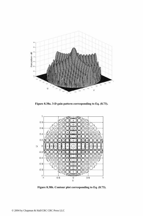
© 200
Figure 8.38a. 3-D gain pattern corresponding to Eq. (8.73).
Figure 8.38b. Contour plot corresponding to Eq. (8.73).
4 by Chapman & Hall/CRC CRC Press LLC

© 200
Figure 8.38c. Three-dimensional plot ( space) corresponding to Eq. (8.73).θ φ,
Figure 8.39a. 3-D gain pattern corresponding to Eq. (8.74).
4 by Chapman & Hall/CRC CRC Press LLC
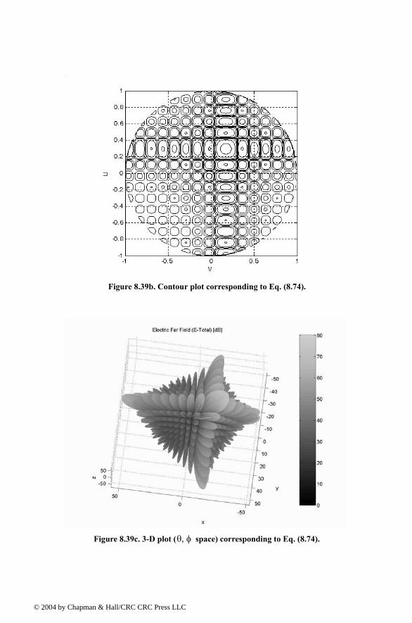
© 200
Figure 8.39b. Contour plot corresponding to Eq. (8.74).
Figure 8.39c. 3-D plot ( space) corresponding to Eq. (8.74).θ φ,
4 by Chapman & Hall/CRC CRC Press LLC
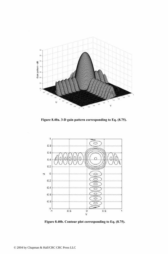
© 200
Figure 8.40a. 3-D gain pattern corresponding to Eq. (8.75).
Figure 8.40b. Contour plot corresponding to Eq. (8.75).
4 by Chapman & Hall/CRC CRC Press LLC

© 200
Figure 8.41a. 3-D gain pattern corresponding to Eq. (8.76).
Figure 8.41b. Contour plot corresponding to Eq. (8.76).
4 by Chapman & Hall/CRC CRC Press LLC
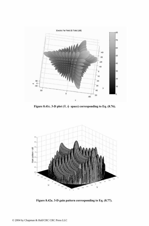
© 200
Figure 8.41c. 3-D plot ( space) corresponding to Eq. (8.76).θ φ,
Figure 8.42a. 3-D gain pattern corresponding to Eq. (8.77).
4 by Chapman & Hall/CRC CRC Press LLC
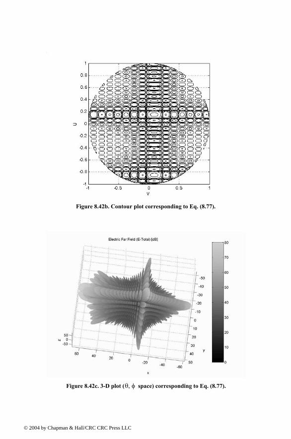
© 200
Figure 8.42b. Contour plot corresponding to Eq. (8.77).
Figure 8.42c. 3-D plot ( space) corresponding to Eq. (8.77).θ φ,
4 by Chapman & Hall/CRC CRC Press LLC
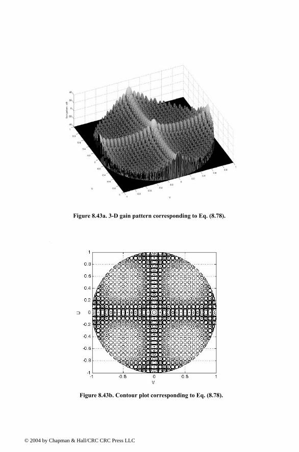
© 200
Figure 8.43a. 3-D gain pattern corresponding to Eq. (8.78).
Figure 8.43b. Contour plot corresponding to Eq. (8.78).
4 by Chapman & Hall/CRC CRC Press LLC
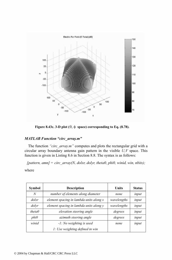
© 200
MATLAB Function circ_array.m
The function circ_array.m computes and plots the rectangular grid with acircular array boundary antenna gain pattern in the visible U,V space. Thisfunction is given in Listing 8.6 in Section 8.8. The syntax is as follows:
[pattern, amn] = circ_array(N, dolxr, dolyr, theta0, phi0, winid, win, nbits);
where
Symbol Description Units Status
N number of elements along diameter none input
dolxr element spacing in lambda units along x wavelengths input
dolyr element spacing in lambda units along y wavelengths input
theta0 elevation steering angle degrees input
phi0 azimuth steering angle degrees input
winid -1: No weighting is used
1: Use weighting defined in win
none input
Figure 8.43c. 3-D plot ( space) corresponding to Eq. (8.78).θ φ,
4 by Chapman & Hall/CRC CRC Press LLC
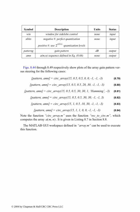
© 200
Figs. 8.44 through 8.49 respectively show plots of the array gain pattern ver-sus steering for the following cases:
[pattern, amn] = circ_array(15, 0.5, 0.5, 0, 0, -1, -1, -3) (8.79)
[pattern, amn] = circ_array(15, 0.5, 0.5, 20, 30, -1, -1, -3) (8.80)
[pattern, amn] = circ_array(15, 0.5, 0.5, 30, 30, 1, Hamming, -3) (8.81)
[pattern, amn] = circ_array(15, 0.5, 0.5, 30, 30, -1, -1, 3) (8.82)
[pattern, amn] = circ_array(15, 1, 0.5, 10, 30, -1, -1, -3) (8.83)
[pattern, amn] = circ_array(15, 1, 1, 0, 0, -1, -1, -3) (8.84)
Note the function circ_array.m uses the function rec_to_circ.m, whichcomputes the array . It is given in Listing 8.7 in Section 8.8.
The MATLAB GUI workspace defined in array.m can be used to executethis function.
win window for sidelobe control none input
nbits negative #: perfect quantization
positive #: use quantization levels
none input
patterng gain pattern dB output
amn a(m,n) sequence defined in Eq. (8.68) none output
Symbol Description Units Status
2nbits
a m n,( )
4 by Chapman & Hall/CRC CRC Press LLC
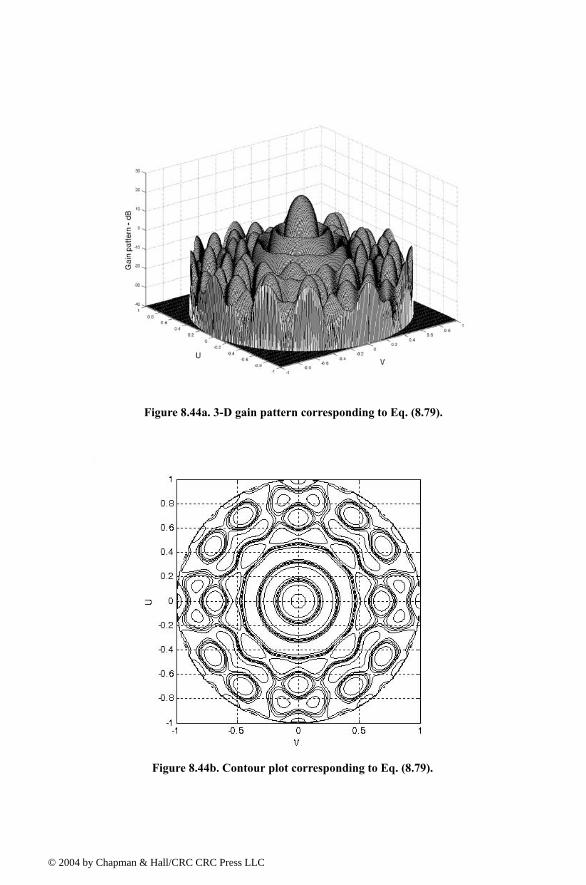
© 200
Figure 8.44a. 3-D gain pattern corresponding to Eq. (8.79).
Figure 8.44b. Contour plot corresponding to Eq. (8.79).
4 by Chapman & Hall/CRC CRC Press LLC
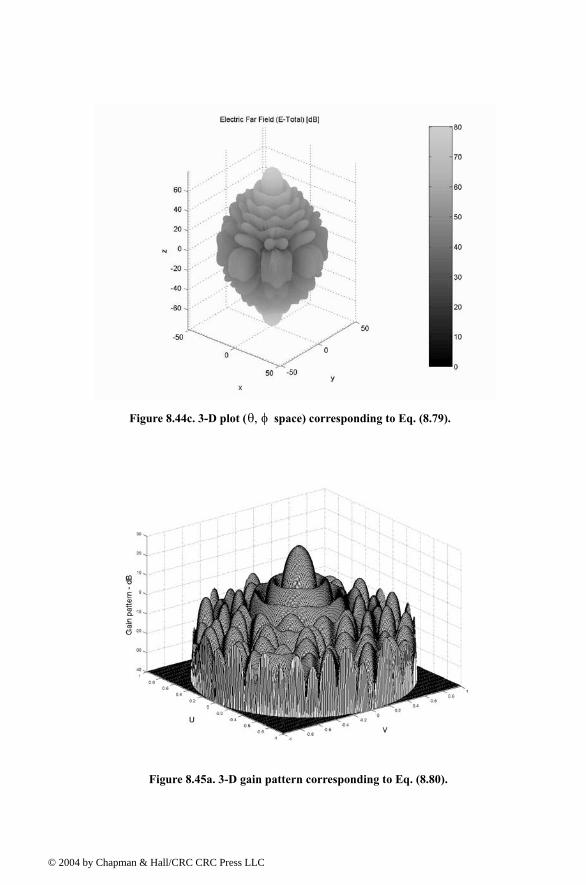
© 200
Figure 8.44c. 3-D plot ( space) corresponding to Eq. (8.79).θ φ,
Figure 8.45a. 3-D gain pattern corresponding to Eq. (8.80).
4 by Chapman & Hall/CRC CRC Press LLC
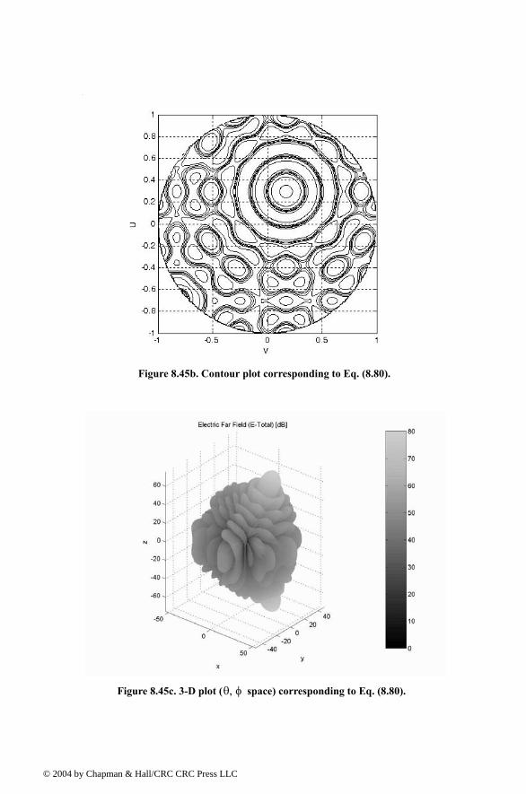
© 200
Figure 8.45b. Contour plot corresponding to Eq. (8.80).
Figure 8.45c. 3-D plot ( space) corresponding to Eq. (8.80).θ φ,
4 by Chapman & Hall/CRC CRC Press LLC
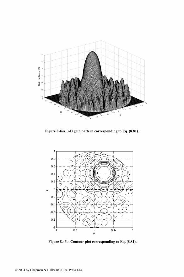
© 200
Figure 8.46a. 3-D gain pattern corresponding to Eq. (8.81).
Figure 8.46b. Contour plot corresponding to Eq. (8.81).
4 by Chapman & Hall/CRC CRC Press LLC
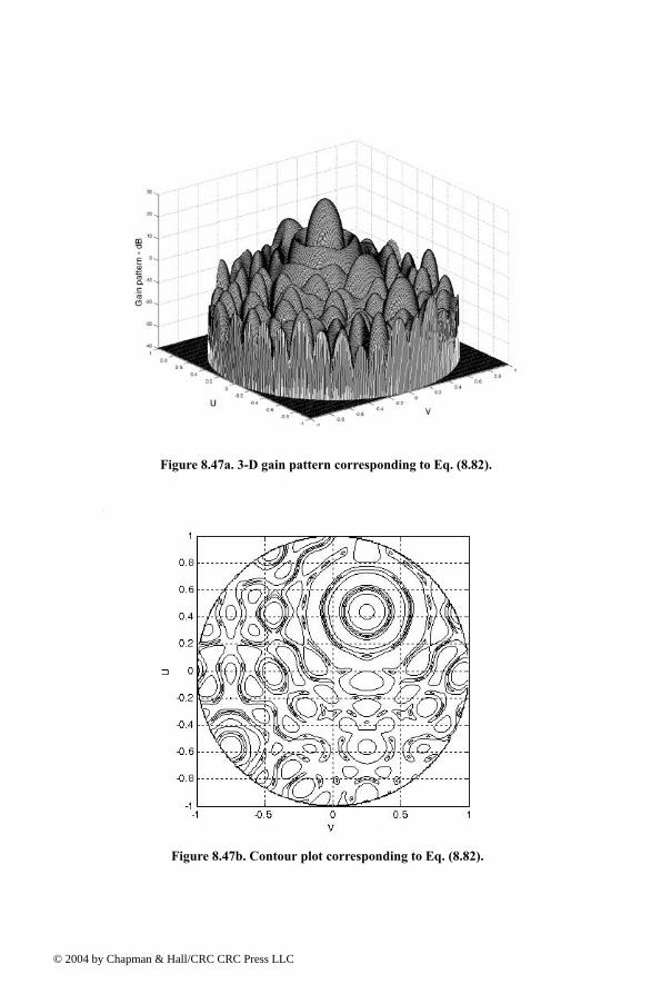
© 200
Figure 8.47a. 3-D gain pattern corresponding to Eq. (8.82).
Figure 8.47b. Contour plot corresponding to Eq. (8.82).
4 by Chapman & Hall/CRC CRC Press LLC
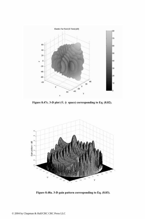
© 200
Figure 8.47c. 3-D plot ( space) corresponding to Eq. (8.82).θ φ,
Figure 8.48a. 3-D gain pattern corresponding to Eq. (8.83).
4 by Chapman & Hall/CRC CRC Press LLC
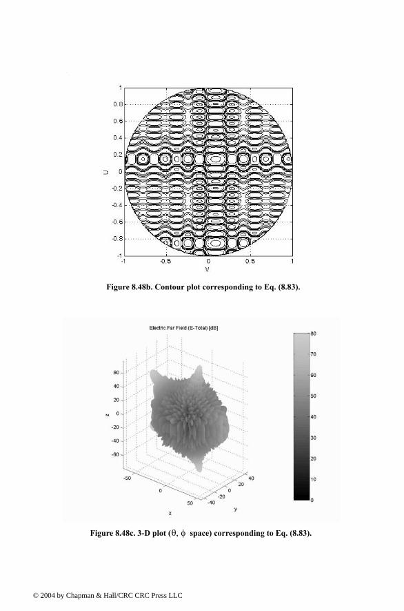
© 200
Figure 8.48b. Contour plot corresponding to Eq. (8.83).
Figure 8.48c. 3-D plot ( space) corresponding to Eq. (8.83).θ φ,
4 by Chapman & Hall/CRC CRC Press LLC
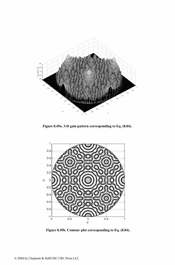
© 200
Figure 8.49a. 3-D gain pattern corresponding to Eq. (8.84).
Figure 8.49b. Contour plot corresponding to Eq. (8.84).
4 by Chapman & Hall/CRC CRC Press LLC
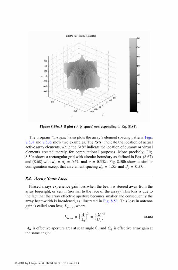
© 200
The program array.m also plots the arrays element spacing pattern. Figs.8.50a and 8.50b show two examples. The xs indicate the location of actualactive array elements, while the os indicate the location of dummy or virtualelements created merely for computational purposes. More precisely, Fig.8.50a shows a rectangular grid with circular boundary as defined in Eqs. (8.67)and (8.68) with and . Fig. 8.50b shows a similarconfiguration except that an element spacing and .
8.6. Array Scan LossPhased arrays experience gain loss when the beam is steered away from the
array boresight, or zenith (normal to the face of the array). This loss is due tothe fact that the array effective aperture becomes smaller and consequently thearray beamwidth is broadened, as illustrated in Fig. 8.51. This loss in antennagain is called scan loss, , where
(8.85)
is effective aperture area at scan angle , and is effective array gain atthe same angle.
Figure 8.49c. 3-D plot ( space) corresponding to Eq. (8.84).θ φ,
dx dy 0.5λ= = a 0.35λ=dx 1.5λ= dy 0.5λ=
Lscan
LscanAAθ------ 2 G
Gθ------ 2
= =
Aθ θ Gθ
4 by Chapman & Hall/CRC CRC Press LLC

© 200
Figure 8.50a. A 15 element circular array made from a rectangular array with circular boundary. Element spacing .dx 0.5λ dy= =
Figure 8.50b. A 15 element circular array made from a rectangular array with circular boundary. Element spacing and .dy 0.5λ= dx 1.5λ=
4 by Chapman & Hall/CRC CRC Press LLC
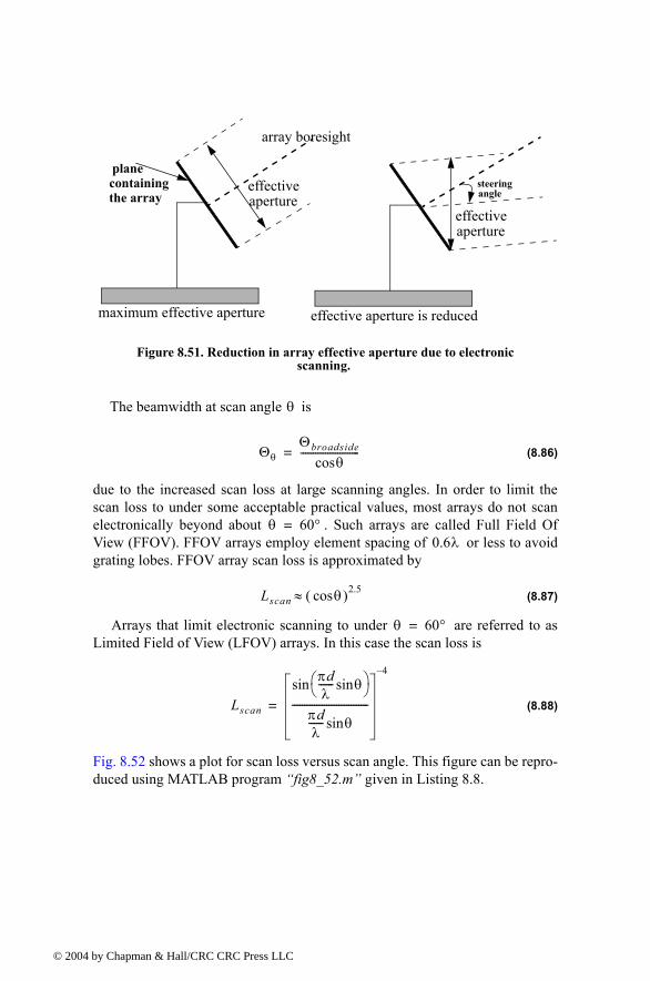
© 200
The beamwidth at scan angle is
(8.86)
due to the increased scan loss at large scanning angles. In order to limit thescan loss to under some acceptable practical values, most arrays do not scanelectronically beyond about . Such arrays are called Full Field OfView (FFOV). FFOV arrays employ element spacing of or less to avoidgrating lobes. FFOV array scan loss is approximated by
(8.87)
Arrays that limit electronic scanning to under are referred to asLimited Field of View (LFOV) arrays. In this case the scan loss is
(8.88)
Fig. 8.52 shows a plot for scan loss versus scan angle. This figure can be repro-duced using MATLAB program fig8_52.m given in Listing 8.8.
maximum effective aperture
array boresight
effective aperture is reduced
effectiveaperture
effectiveaperture
Figure 8.51. Reduction in array effective aperture due to electronic scanning.
plane containingthe array
steeringangle
θ
ΘθΘbroadside
θcos------------------------=
θ 60°=0.6λ
Lscan θcos( )2.5≈
θ 60°=
Lscan
πdλ
------ θsin sin
πdλ
------ θsin-------------------------------
4
=
4 by Chapman & Hall/CRC CRC Press LLC
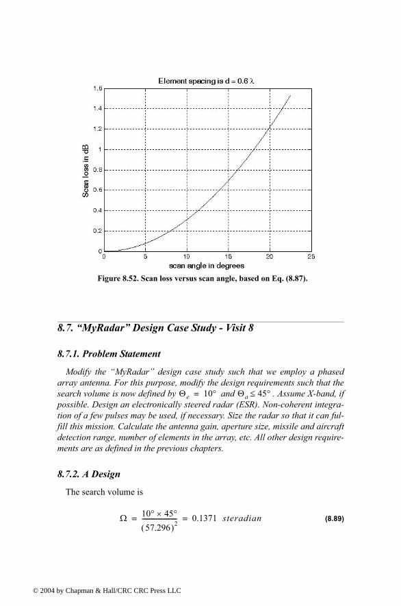
© 200
8.7. MyRadar Design Case Study - Visit 8
8.7.1. Problem Statement
Modify the MyRadar design case study such that we employ a phasedarray antenna. For this purpose, modify the design requirements such that thesearch volume is now defined by and . Assume X-band, ifpossible. Design an electronically steered radar (ESR). Non-coherent integra-tion of a few pulses may be used, if necessary. Size the radar so that it can ful-fill this mission. Calculate the antenna gain, aperture size, missile and aircraftdetection range, number of elements in the array, etc. All other design require-ments are as defined in the previous chapters.
8.7.2. A Design
The search volume is
(8.89)
Figure 8.52. Scan loss versus scan angle, based on Eq. (8.87).
Θe 10°= Θa 45°≤
Ω 10° 45°×
57.296( )2----------------------- 0.1371 steradian= =
4 by Chapman & Hall/CRC CRC Press LLC
© 200
For an X-band radar, choose , then
(8.90)
Assume an aperture size ; thus
(8.91)
Assume square aperture. It follows that the aperture 3-dB beamwidth is cal-culated from
(8.92)
The number of beams required to fill the search volume is
(8.93)
Note that the packing factor is used to allow for beam overlap in order toavoid gaps in the beam coverage. The search scan rate is 2 seconds. Thus, theminimum PRF should correspond to 200 beams per second (i.e., ).This PRF will allow the radar to visit each beam position only once during acomplete scan.
It was determined in Chapter 2 that 4-pulse non-coherent integration alongwith a cumulative detection scheme are required to achieve the desired proba-bility of detection. It was also determined that the single pulse energy for themissile and aircraft cases are respectively given by (see page 118)
(8.94)
(8.95)
However, these values were derived using and . Thenew wavelength is and the new gain is . Thus,the missile and aircraft single pulse energy, assuming the same single pulseSNR as derived in Chapter 2 (i.e., ) are
(8.96)
fo 9GHz=
λ 3 108×
9 109×----------------- 0.0333m= =
Ae 2.25m2=
G4πAe
λ2------------ 4 π 2.25××
0.0333( )2----------------------------- 25451.991 G⇒ 44dB= = = =
G 4πθ3db
2----------=
θ3dB⇒ 4 π 1802××
25451.991 π2×------------------------------------- 1.3°= =
nb kpΩ
1.3 57.296⁄( )2-----------------------------------
kp 1.5=
nb⇒ 399.5 choose nb⇒ 400= = =
kp
fr 200Hz=
Em 0.1147Joules=
Ea 0.1029Joules=
λ 0.1m= G 2827.4=λ 0.0333m= G 25451.99=
SNR 4dB=
Em 0.1147 0.12 2827.42×
0.03332 254522×------------------------------------------× 0.012765Joules= =
4 by Chapman & Hall/CRC CRC Press LLC
© 200
(8.97)
The single pulse peak power that will satisfy detection for both target typesis
(8.98)
where is used.
Note that since a 4-pulse non-coherent integration is adopted, the minimumPRF is increased to
(8.99)
and the total number of beams is . Consequently the unambiguousrange is
(8.100)
(1.101)
Since the effective aperture is , then by assuming an array effi-
ciency the actual array size is
(8.102)
It follows that the physical array sides are . Thus, by selectingthe array element spacing an array of size elements satis-fies the design requirements.
Since the field of view is less than , one can use element spacing aslarge as without introducing any grating lobes into the array FOV.Using this option yields an array of size elements. Hence, therequired power per element is less than .
8.8. MATLAB Program and Function ListingsThis section contains listings of all MATLAB programs and functions used
in this chapter. Users are encouraged to rerun this code with different inputs inorder to enhance their understanding of the theory.
Ea 0.1029 0.12 2827.42×
0.03332 254522×------------------------------------------× 0.01145Joules= =
Pt0.01276520 10 6×---------------------- 638.25W= =
τ 20µs=
fr 200 4× 800Hz= =
nb 1600=
Ru3 108×2 800×------------------≤ 187.5Km=
Ae 2.25m2=
ρ 0.8=
A 2.250.8---------- 2.8125m2= =
1.68m 1.68m×d 0.6λ= 84 84×
22.5°±d 1.5λ=
34 34× 1156=0.6W
4 by Chapman & Hall/CRC CRC Press LLC
© 200
Listing 8.1. MATLAB Program fig8_5.m% Use this code to produce figure 8.5a and 8.5b based on equation 8.34clear allclose alleps = 0.00001;k = 2*pi;theta = -pi : pi / 10791 : pi;var = sin(theta);nelements = 8;d = 1; % d = 1;num = sin((nelements * k * d * 0.5) .* var);
if(abs(num) <= eps) num = eps;endden = sin((k* d * 0.5) .* var);if(abs(den) <= eps) den = eps;end
pattern = abs(num ./ den);maxval = max(pattern);pattern = pattern ./ maxval;
figure(1)plot(var,pattern)xlabel('sine angle - dimensionless')ylabel('Array pattern')grid
figure(2)plot(var,20*log10(pattern))axis ([-1 1 -60 0])xlabel('sine angle - dimensionless')ylabel('Power pattern [dB]')grid;
figure(3)theta = theta +pi/2;polar(theta,pattern)title ('Array pattern')
figure(4)
4 by Chapman & Hall/CRC CRC Press LLC
© 200
polardb(theta,pattern)title ('Power pattern [dB]')
Listing 8.2. MATLAB Program fig8_7.m% Use this program to reproduce Fig. 8.7 of textclear allclose alleps =0.00001;N = 32;rect(1:32) = 1;ham = hamming(32);han = hanning(32);blk = blackman(32);k3 = kaiser(32,3);k6 = kaiser(32,6);RECT = 20*log10(abs(fftshift(fft(rect, 512)))./32 +eps);HAM = 20*log10(abs(fftshift(fft(ham, 512)))./32 +eps);HAN = 20*log10(abs(fftshift(fft(han, 512)))./32+eps);BLK = 20*log10(abs(fftshift(fft(blk, 512)))./32+eps);K6 = 20*log10(abs(fftshift(fft(k6, 512)))./32+eps);x = linspace(-1,1,512);figuresubplot(2,1,1)plot(x,RECT,'k--',x,HAM,'k',x,HAN,'k-.');xlabel('x')ylabel('Window')gridaxis tightlegend('Rectangular','Hamming','Hanning')subplot(2,1,2)plot(x,RECT,'k--',x,BLK,'k',x,K6,'K-.')xlabel('x')ylabel('Window')legend('Rectangular','Blackman','Kasier at \beta = 6')gridaxis tight
Listing 8.3. MATLAB Function linear_array.mfunction [theta,patternr,patterng] = linear_array(Nr,dolr,theta0,winid,win,nbits);% This function computes and returns the gain radiation pattern for a linear array
4 by Chapman & Hall/CRC CRC Press LLC
© 200
% It uses the FFT to compute the pattern%%%%%%%%% ********** INPUTS *********** %%%%%%%%%%% Nr ==> number of elements; dolr ==> element spacing (d) in lambda units divided by lambda% theta0 ==> steering angle in degrees; winid ==> use winid negative for no window, winid positive to enter your window of size(Nr)% win is input window, NOTE that win must be an NrX1 row vector; nbits ==> number of bits used in the phase shifters% negative nbits mean no quantization is used%%%%%% *********** OUTPUTS *********** %%%%%%%%%%%%% theta ==> real-space angle; patternr ==> array radiation pattern in dBs% patterng ==> array directive gain pattern in dBs%%%%%%%%%%%% **************** %%%%%%%%%%%%eps = 0.00001;n = 0:Nr-1;i = sqrt(-1);%if dolr is > 0.5 then; choose dol = 0.25 and compute new Nif(dolr <=0.5) dol = dolr; N = Nr;else ratio = ceil(dolr/.25); N = Nr * ratio; dol = 0.25;end% choose proper size fft, for minimum value choose 256Nrx = 10 * N; nfft = 2^(ceil(log(Nrx)/log(2)));if nfft < 256 nfft = 256;end% convert steering angle into radians; and compute the sine of angletheta0 = theta0 *pi /180.;sintheta0 = sin(theta0);% determine and compute quantized steering angleif nbits < 0 phase0 = exp(i*2.0*pi .* n * dolr * sintheta0);else % compute and add the phase shift terms (WITH nbits quantization) % Use formula thetal = (2*pi*n*dol) * sin(theta0) divided into 2^nbits % and rounded to the nearest qunatization level levels = 2^nbits; qlevels = 2.0 * pi / levels; % compute quantization levels
4 by Chapman & Hall/CRC CRC Press LLC
© 200
% compute the phase level and round it to the closest quantization level at each array element angleq = round(dolr .* n * sintheta0 * levels) .* qlevels; % vector of possi-ble angles phase0 = exp(i*angleq);end% generate array of elements with or without windowif winid < 0 wr(1:Nr) = 1;else wr = win';end% add the phase shift terms wr = wr .* phase0; % determine if interpolation is needed (i.e., N > Nr)if N > Nr w(1:N) = 0; w(1:ratio:N) = wr(1:Nr);else w = wr;end% compute the sine(theta) in real space that corresponds to the FFT index arg = [-nfft/2:(nfft/2)-1] ./ (nfft*dol);idx = find(abs(arg) <= 1);sinetheta = arg(idx);theta = asin(sinetheta);% convert angle into degreestheta = theta .* (180.0 / pi);% Compute fft of w (radiation pattern)patternv = (abs(fftshift(fft(w,nfft)))).^2;% convert radiationa pattern to dBspatternr = 10*log10(patternv(idx) ./Nr + eps);% Compute directive gain pattern rbarr = 0.5 *sum(patternv(idx)) ./ (nfft * dol);patterng = 10*log10(patternv(idx) + eps) - 10*log10(rbarr + eps);return
Listing 8.4. MATLAB Program circular_array.m% Circular Array in the x-y plane % Element is a short dipole antenna parallel to the z axis% 2D Radiation Patterns for fixed phi or fixed theta% dB polar plots uses the polardb.m file% Last modified: July 13, 2003
4 by Chapman & Hall/CRC CRC Press LLC
© 200
%%%%% Element expression needs to be modified if different%%%% than a short dipole antenna along the z axisclear allclf% close all% ==== Input Parameters ====a = 1.; % radius of the circleN = 20; % number of Elements of the circular arraytheta0 = 45; % main beam Theta directionphi0 = 60; % main beam Phi direction% Theta or Phi variations for the calculations of the far field patternVariations = 'Phi'; % Correct selections are 'Theta' or 'Phi' phid = 60; % constant phi plane for theta variationsthetad = 45; % constant theta plane for phi variations% ==== End of Input parameters section ====dtr = pi/180; % conversion factorsrtd = 180/pi;phi0r = phi0*dtr;theta0r = theta0*dtr;lambda = 1; k = 2*pi/lambda;ka = k*a; % Wavenumber times the radiusjka = j*ka;I(1:N) = 1; % Elements excitation Amplitude and Phasealpha(1:N) =0; for n = 1:N % Element positions Uniformly distributed along the circle phin(n) = 2*pi*n/N;endswitch Variationscase 'Theta' phir = phid*dtr; % Pattern in a constant Phi plane i = 0; for theta = 0.001:1:181 i = i+1; thetar(i) = theta*dtr; angled(i) = theta; angler(i) = thetar(i); Arrayfactor(i) = 0; for n = 1:N Arrayfactor(i) = Arrayfactor(i) + I(n)*exp(j*alpha(n)) ... * exp( jka*(sin(thetar(i))*cos(phir -phin(n))) ... -jka*(sin(theta0r )*cos(phi0r-phin(n))) ); end Arrayfactor(i) = abs(Arrayfactor(i));
4 by Chapman & Hall/CRC CRC Press LLC

© 200
Element(i) = abs(sin(thetar(i)+0*dtr)); % use the abs function to avoid endcase 'Phi' thetar = thetad*dtr; % Pattern in a constant Theta plane i = 0; for phi = 0.001:1:361 i = i+1; phir(i) = phi*dtr; angled(i) = phi; angler(i) = phir(i); Arrayfactor(i) = 0; for n = 1:N Arrayfactor(i) = Arrayfactor(i) + I(n)*exp(j*alpha(n)) ... * exp( jka*(sin(thetar )*cos(phir(i)-phin(n))) ... -jka*(sin(theta0r)*cos(phi0r -phin(n))) ); end Arrayfactor(i) = abs(Arrayfactor(i)); Element(i) = abs(sin(thetar+0*dtr)); % use the abs function to avoid end endangler = angled*dtr;Element = Element/max(Element);Array = Arrayfactor/max(Arrayfactor);ArraydB = 20*log10(Array);EtotalR =(Element.*Arrayfactor)/max(Element.*Arrayfactor);figure(1)plot(angled,Array)ylabel('Array pattern')gridswitch Variationscase 'Theta' axis ([0 180 0 1 ])% theta = theta +pi/2; xlabel('Theta [Degrees]') title ( 'phi = 90^o plane')case 'Phi'axis ([0 360 0 1 ]) xlabel('Phi [Degrees]') title ( 'Theta = 90^o plane')endfigure(2)plot(angled,ArraydB)%axis ([-1 1 -60 0])ylabel('Power pattern [dB]')grid;
4 by Chapman & Hall/CRC CRC Press LLC
© 200
switch Variationscase 'Theta' axis ([0 180 -60 0 ]) xlabel('Theta [Degrees]') title ( 'phi = 90^o plane')case 'Phi'axis ([0 360 -60 0 ]) xlabel('Phi [Degrees]') title ( 'Theta = 90^o plane')endfigure(3)polar(angler,Array)title ('Array pattern')figure(4)polardb(angler,Array)title ('Power pattern [dB]')% the plots provided above are for the array factor based on the circular % array plots for other patterns such as those for the antenna element % (Element)or the total pattern (Etotal based on Element*Arrayfactor) can % also be displayed by the user as all these patterns are already computed % above.figure(10)subplot(2,2,1) polardb (angler,Element,'b-'); % rectangular plot of element patterntitle('Element normalized E field [dB]')subplot(2,2,2)polardb(angler,Array,'b-')title(' Array Factor normalized [dB]')subplot(2,2,3)polardb(angler,EtotalR,'b-'); % polar plottitle('Total normalized E field [dB]')%%%%%%%%%%%%%%%%%%%%%%%%%%%%%%%%%%%%%%%%%%%%%%%%%%%%function polardb(theta,rho,line_style)% POLARDB Polar coordinate plot.% POLARDB(THETA, RHO) makes a plot using polar coordinates of% the angle THETA, in radians, versus the radius RHO in dB.% The maximum value of RHO should not exceed 1. It should not be% normalized, however (i.e., its max. value may be less than 1).% POLAR(THETA,RHO,S) uses the linestyle specified in string S.% See PLOT for a description of legal linestyles.if nargin < 1 error('Requires 2 or 3 input arguments.')elseif nargin == 2
4 by Chapman & Hall/CRC CRC Press LLC
© 200
if isstr(rho) line_style = rho; rho = theta; [mr,nr] = size(rho); if mr == 1 theta = 1:nr; else th = (1:mr)'; theta = th(:,ones(1,nr)); end else line_style = 'auto'; endelseif nargin == 1 line_style = 'auto'; rho = theta; [mr,nr] = size(rho); if mr == 1 theta = 1:nr; else th = (1:mr)'; theta = th(:,ones(1,nr)); endendif isstr(theta) | isstr(rho) error('Input arguments must be numeric.');endif ~isequal(size(theta),size(rho)) error('THETA and RHO must be the same size.');end% get hold statecax = newplot;next = lower(get(cax,'NextPlot'));hold_state = ishold;
% get x-axis text color so grid is in same colortc = get(cax,'xcolor');ls = get(cax,'gridlinestyle');% Hold on to current Text defaults, reset them to the% Axes' font attributes so tick marks use them.fAngle = get(cax, 'DefaultTextFontAngle');fName = get(cax, 'DefaultTextFontName');fSize = get(cax, 'DefaultTextFontSize');fWeight = get(cax, 'DefaultTextFontWeight');
4 by Chapman & Hall/CRC CRC Press LLC
© 200
fUnits = get(cax, 'DefaultTextUnits');set(cax, 'DefaultTextFontAngle', get(cax, 'FontAngle'), ... 'DefaultTextFontName', get(cax, 'FontName'), ... 'DefaultTextFontSize', get(cax, 'FontSize'), ... 'DefaultTextFontWeight', get(cax, 'FontWeight'), ... 'DefaultTextUnits','data')% make a radial grid hold on; maxrho =1; hhh=plot([-maxrho -maxrho maxrho maxrho],[-maxrho maxrho maxrho -maxrho]); set(gca,'dataaspectratio',[1 1 1],'plotboxaspectratiomode','auto') v = [get(cax,'xlim') get(cax,'ylim')]; ticks = sum(get(cax,'ytick')>=0); delete(hhh);% check radial limits and ticks rmin = 0; rmax = v(4); rticks = max(ticks-1,2); if rticks > 5 % see if we can reduce the number if rem(rticks,2) == 0 rticks = rticks/2; elseif rem(rticks,3) == 0 rticks = rticks/3; end end% only do grids if hold is offif ~hold_state% define a circle th = 0:pi/50:2*pi; xunit = cos(th); yunit = sin(th);% now really force points on x/y axes to lie on them exactly inds = 1:(length(th)-1)/4:length(th); xunit(inds(2:2:4)) = zeros(2,1); yunit(inds(1:2:5)) = zeros(3,1);% plot background if necessary if ~isstr(get(cax,'color')), patch('xdata',xunit*rmax,'ydata',yunit*rmax, ... 'edgecolor',tc,'facecolor',get(gca,'color'),... 'handlevisibility','off'); end% draw radial circles with dB ticks c82 = cos(82*pi/180); s82 = sin(82*pi/180); rinc = (rmax-rmin)/rticks;
4 by Chapman & Hall/CRC CRC Press LLC
© 200
tickdB=-10*(rticks-1); % the innermost tick dB value for i=(rmin+rinc):rinc:rmax hhh = plot(xunit*i,yunit*i,ls,'color',tc,'linewidth',1,... 'handlevisibility','off'); text((i+rinc/20)*c82*0,-(i+rinc/20)*s82, ... [' ' num2str(tickdB) ' dB'],'verticalalignment','bottom',... 'handlevisibility','off') tickdB=tickdB+10; end set(hhh,'linestyle','-') % Make outer circle solid% plot spokes th = (1:6)*2*pi/12; cst = cos(th); snt = sin(th); cs = [-cst; cst]; sn = [-snt; snt]; plot(rmax*cs,rmax*sn,ls,'color',tc,'linewidth',1,... 'handlevisibility','off')% annotate spokes in degrees rt = 1.1*rmax; for i = 1:length(th) text(rt*cst(i),rt*snt(i),int2str(i*30),... 'horizontalalignment','center',... 'handlevisibility','off'); if i == length(th) loc = int2str(0); else loc = int2str(180+i*30); end text(-rt*cst(i),-rt*snt(i),loc,'horizontalalignment','center',... 'handlevisibility','off') end% set view to 2-D view(2);% set axis limits axis(rmax*[-1 1 -1.15 1.15]);end% Reset defaults.set(cax, 'DefaultTextFontAngle', fAngle , ... 'DefaultTextFontName', fName , ... 'DefaultTextFontSize', fSize, ... 'DefaultTextFontWeight', fWeight, ... 'DefaultTextUnits', fUnits );% Transfrom data to dB scalermin = 0; rmax=1;
4 by Chapman & Hall/CRC CRC Press LLC
© 200
rinc = (rmax-rmin)/rticks;rhodb=zeros(1,length(rho));for i=1:length(rho) if rho(i)==0 rhodb(i)=0; else rhodb(i)=rmax+2*log10(rho(i))*rinc; end if rhodb(i)<=0 rhodb(i)=0; endend% transform data to Cartesian coordinates.xx = rhodb.*cos(theta);yy = rhodb.*sin(theta);% plot data on top of gridif strcmp(line_style,'auto') q = plot(xx,yy);else q = plot(xx,yy,line_style);endif nargout > 0 hpol = q;endif ~hold_state set(gca,'dataaspectratio',[1 1 1]), axis off; set(cax,'NextPlot',next);endset(get(gca,'xlabel'),'visible','on')set(get(gca,'ylabel'),'visible','on')
Listing 8.5. MATLAB Function rect_array.mfunction [pattern] = rect_array(Nxr,Nyr,dolxr,dolyr,theta0,phi0,winid,win,nbits);%%%%%%%%%% ************************ %%%%%%%%%%% This function computes the 3-D directive gain patterns for a planar array% This function uses the fft2 to compute its output%%%%%%%% ************ INPUTS ************ %%%%%%%%%% Nxr ==> number of along x-axis; Nyr ==> number of elements along y-axis% dolxr ==> element spacing in x-direction; dolyr ==> element spacing in y-direction Both are in lambda units% theta0 ==> elevation steering angle in degrees, phi0 ==> azimuth steering angle in degrees
4 by Chapman & Hall/CRC CRC Press LLC
© 200
% winid ==> window identifier; winid negative ==> no window ; winid posi-tive ==> use window given by win% win ==> input window function (2-D window) MUST be of size (Nxr X Nyr)% nbits is the number of nbits used in phase quantization; nbits negative ==> NO quantization%%%%% *********** OUTPUTS ************* %%%%%%%% pattern ==> directive gain pattern%%%%%%% ************************ %%%%%%%%%%%%eps = 0.0001;nx = 0:Nxr-1;ny = 0:Nyr-1;i = sqrt(-1);% check that window size is the same as the array size[nw,mw] = size(win);if winid >0 if nw ~= Nxr fprintf('STOP == Window size must be the same as the array') returnendif mw ~= Nyr fprintf('STOP == Window size must be the same as the array') returnendend
%if dol is > 0.5 then; choose dol = 0.5 and compute new Nif(dolxr <=0.5) ratiox = 1 ; dolx = dolxr ; Nx = Nxr ;else ratiox = ceil(dolxr/.5) ; Nx = (Nxr -1 ) * ratiox + 1 ; dolx = 0.5 ;endif(dolyr <=0.5) ratioy = 1 ; doly = dolyr ; Ny = Nyr ;else ratioy = ceil(dolyr/.5) ; Ny = (Nyr -1) * ratioy + 1 ; doly = 0.5 ;end
4 by Chapman & Hall/CRC CRC Press LLC
© 200
% choose proper size fft, for minimum value choose 256X256Nrx = 10 * Nx; Nry = 10 * Ny;nfftx = 2^(ceil(log(Nrx)/log(2)));nffty = 2^(ceil(log(Nry)/log(2)));if nfftx < 256 nfftx = 256;endif nffty < 256 nffty = 256;end% generate array of elements with or without windowif winid < 0 array = ones(Nxr,Nyr);else array = win;end% convert steering angles (theta0, phi0) to radianstheta0 = theta0 * pi / 180;phi0 = phi0 * pi / 180;% convert steering angles (theta0, phi0) to U-V sine-spaceu0 = sin(theta0) * cos(phi0);v0 = sin(theta0) * sin(phi0);% Use formula thetal = (2*pi*n*dol) * sin(theta0) divided into 2^m levels% and rounded to the nearest qunatization levelif nbits < 0 phasem = exp(i*2*pi*dolx*u0 .* nx *ratiox); phasen = exp(i*2*pi*doly*v0 .* ny *ratioy);else levels = 2^nbits; qlevels = 2.0*pi / levels; % compute quantization levels sinthetaq = round(dolx .* nx * u0 * levels * ratiox) .* qlevels; % vector of possible angles sinphiq = round(doly .* ny * v0 * levels *ratioy) .* qlevels; % vector of pos-sible angles phasem = exp(i*sinthetaq); phasen = exp(i*sinphiq); end% add the phase shift termsarray = array .* (transpose(phasem) * phasen);% determine if interpolation is needed (i.e., N > Nr)if (Nx > Nxr )| (Ny > Nyr) for xloop = 1 : Nxr temprow = array(xloop, :) ;
4 by Chapman & Hall/CRC CRC Press LLC
© 200
w( (xloop-1)*ratiox+1, 1:ratioy:Ny) = temprow ; end array = w;else w = array ;% w(1:Nx, :) = array(1:N,:);end% Compute array patternarrayfft = abs(fftshift(fft2(w,nfftx,nffty))).^2 ;%compute [su,sv] matrixU = [-nfftx/2:(nfftx/2)-1] ./(dolx*nfftx);indexx = find(abs(U) <= 1);U = U(indexx);V = [-nffty/2:(nffty/2)-1] ./(doly*nffty);indexy = find(abs(V) <= 1);V = V(indexy);%Normalize to generate gain paternrbar=sum(sum(arrayfft(indexx,indexy))) / dolx/doly/4./nfftx/nffty;arrayfft = arrayfft(indexx,indexy) ./rbar;[SU,SV] = meshgrid(V,U);indx = find((SU.^2 + SV.^2) >1);arrayfft(indx) = eps/10;pattern = 10*log10(arrayfft +eps);figure(1)mesh(V,U,pattern);xlabel('V')ylabel('U');zlabel('Gain pattern - dB')figure(2)contour(V,U,pattern)gridaxis imagexlabel('V')ylabel('U');axis([-1 1 -1 1])figure(3)x0 = (Nx+1)/2 ;y0 = (Ny+1)/2 ;radiusx = dolx*((Nx-1)/2) ;radiusy = doly*((Ny-1)/2) ;[xxx, yyy]=find(abs(array)>eps);xxx = xxx-x0 ;yyy = yyy-y0 ;plot(yyy*doly, xxx*dolx,'rx')
4 by Chapman & Hall/CRC CRC Press LLC
© 200
hold onaxis([-radiusy-0.5 radiusy+0.5 -radiusx-0.5 radiusx+0.5]);gridtitle('antenna spacing pattern');xlabel('y - \lambda units')ylabel('x - \lambda units')[xxx0, yyy0]=find(abs(array)<=eps);xxx0 = xxx0-x0 ;yyy0 = yyy0-y0 ;plot(yyy0*doly, xxx0*dolx,'co')axis([-radiusy-0.5 radiusy+0.5 -radiusx-0.5 radiusx+0.5]);hold offreturn
Listing 8.6. MATLAB Function circ_array.mfunction [pattern,amn] = circ_array(N,dolxr,dolyr,theta0,phi0,winid,win,nbits);%%%%%%%%% ************************ %%%%%%%%%%%% This function computes the 3-D directive gain patterns for a circular planar array% This function uses the fft2 to compute its output. It assumes that there are the same number of elements along the major x- and y-axes%%%%%%%% ************ INPUTS ************ %%%%%%%%% N ==> number of elements along x-aixs or y-axis% dolxr ==> element spacing in x-direction; dolyr ==> element spacing in y-direction. Both are in lambda units% theta0 ==> elevation steering angle in degrees, phi0 ==> azimuth steering angle in degrees% This function uses the function (rec_to_circ) which computes the circular array from a square % array (of size NXN) using the notation developed by ALLEN,J.L.,"The The-ory of Array Antennas % (with Emphasis on Radar Application)" MIT-LL Technical Report No. 323, July, 25 1965. % winid ==> window identifier; winid negative ==> no window ; winid posi-tive ==> use window given by win% win ==> input window function (2-D window) MUST be of size (Nxr X Nyr)% nbits is the number of nbits used in phase quantization; nbits negative ==> NO quantization%%%%%%% *********** OUTPUTS ************* %%%%%%%%% amn ==> array of ones and zeros; ones indicate true element location on the grid% zeros mean no elements at that location; pattern ==> directive gain pattern
4 by Chapman & Hall/CRC CRC Press LLC

© 200
%%%%%%%%% ************************ %%%%%%%%%%%%eps = 0.0001;nx = 0:N-1;ny = 0:N-1;i = sqrt(-1);% check that window size is the same as the array size[nw,mw] = size(win);if winid >0 if mw ~= N fprintf('STOP == Window size must be the same as the array') return end if nw ~= N fprintf('STOP == Window size must be the same as the array') return endend%if dol is > 0.5 then; choose dol = 0.5 and compute new Nif(dolxr <=0.5) ratiox = 1 ; dolx = dolxr ; Nx = N ;else ratiox = ceil(dolxr/.5) ; Nx = (N-1) * ratiox + 1 ; dolx = 0.5 ;endif(dolyr <=0.5) ratioy = 1 ; doly = dolyr ; Ny = N ;else ratioy = ceil(dolyr/.5); Ny = (N-1)*ratioy + 1 ; doly = 0.5 ;end% choose proper size fft, for minimum value choose 256X256Nrx = 10 * Nx; Nry = 10 * Ny;nfftx = 2^(ceil(log(Nrx)/log(2)));nffty = 2^(ceil(log(Nry)/log(2)));if nfftx < 256 nfftx = 256;end
4 by Chapman & Hall/CRC CRC Press LLC
© 200
if nffty < 256 nffty = 256;end% generate array of elements with or without windowif winid < 0 array = ones(N,N);else array = win;end% convert steering angles (theta0, phi0) to radianstheta0 = theta0 * pi / 180;phi0 = phi0 * pi / 180;% convert steering angles (theta0, phi0) to U-V sine-spaceu0 = sin(theta0) * cos(phi0);v0 = sin(theta0) * sin(phi0);% Use formula thetal = (2*pi*n*dol) * sin(theta0) divided into 2^m levels% and rounded to the nearest qunatization levelif nbits < 0 phasem = exp(i*2*pi*dolx*u0 .* nx * ratiox); phasen = exp(i*2*pi*doly*v0 .* ny * ratioy);else levels = 2^nbits; qlevels = 2.0*pi / levels; % compute quantization levels sinthetaq = round(dolx .* nx * u0 * levels * ratiox) .* qlevels; % vector of possible angles sinphiq = round(doly .* ny * v0 * levels *ratioy) .* qlevels; % vector of pos-sible angles phasem = exp(i*sinthetaq); phasen = exp(i*sinphiq); end% add the phase shift termsarray = array .* (transpose(phasem) * phasen) ;
% determine if interpolation is needed (i.e., N > Nr)if (Nx > N )| (Ny > N) for xloop = 1 : N temprow = array(xloop, :) ; w( (xloop-1)*ratiox+1, 1:ratioy:Ny) = temprow ; end array = w;else w(1:Nx, :) = array(1:N,:);end% Convert rectangular array into circular using function rec_to_circ
4 by Chapman & Hall/CRC CRC Press LLC
© 200
[m,n] = size(w) ;NC = max(m,n); % Use Allens algorithmif Nx == Ny temp_array = w;else midpoint = (NC-1)/2 +1 ; midwm = (m-1)/2 ; midwn = (n-1)/2 ; temp_array = zeros(NC,NC); temp_array(midpoint-midwm:midpoint+midwm, midpoint-midwn:mid-point+midwn) = w ;endamn = rec_to_circ(NC); % must be rectangular array (Nx=Ny)amn = temp_array .* amn ;
% Compute array patternarrayfft = abs(fftshift(fft2(amn,nfftx,nffty))).^2 ;%compute [su,sv] matrixU = [-nfftx/2:(nfftx/2)-1] ./(dolx*nfftx);indexx = find(abs(U) <= 1);U = U(indexx);V = [-nffty/2:(nffty/2)-1] ./(doly*nffty);indexy = find(abs(V) <= 1);V = V(indexy);[SU,SV] = meshgrid(V,U);indx = find((SU.^2 + SV.^2) >1);arrayfft(indx) = eps/10;%Normalize to generate gain patternrbar=sum(sum(arrayfft(indexx,indexy))) / dolx/doly/4./nfftx/nffty;arrayfft = arrayfft(indexx,indexy) ./rbar;[SU,SV] = meshgrid(V,U);indx = find((SU.^2 + SV.^2) >1);arrayfft(indx) = eps/10;pattern = 10*log10(arrayfft +eps);figure(1)mesh(V,U,pattern);xlabel('V')ylabel('U');zlabel('Gain pattern - dB')figure(2)contour(V,U,pattern)axis imagegridxlabel('V')
4 by Chapman & Hall/CRC CRC Press LLC
© 200
ylabel('U');axis([-1 1 -1 1])figure(3)x0 = (NC+1)/2 ;y0 = (NC+1)/2 ;radiusx = dolx*((NC-1)/2 + 0.05/dolx) ;radiusy = doly*((NC-1)/2 + 0.05/dolx) ;theta = 5 ;[xxx, yyy]=find(abs(amn)>0);xxx = xxx-x0 ;yyy = yyy-y0 ;plot(yyy*doly, xxx*dolx,'rx')axis equalhold onaxis([-radiusy-0.5 radiusy+0.5 -radiusx-0.5 radiusx+0.5]);gridtitle('antenna spacing pattern');xlabel('y - \lambda units')ylabel('x - \lambda units')[x, y]= makeellip( 0, 0, radiusx, radiusy, theta) ;plot(y, x) ;axis([-radiusy-0.5 radiusy+0.5 -radiusx-0.5 radiusx+0.5]);[xxx0, yyy0]=find(abs(amn)<=0);xxx0 = xxx0-x0 ;yyy0 = yyy0-y0 ;plot(yyy0*doly, xxx0*dolx,'co')axis([-radiusy-0.5 radiusy+0.5 -radiusx-0.5 radiusx+0.5]);axis equalhold off ;return
Listing 8.7. MATLAB Function rec_to_circ.mfunction amn = rec_to_circ(N)midpoint = (N-1)/2 + 1;amn = zeros(N);array1(midpoint,midpoint) = N;x0 = midpoint;y0 = x0;for i = 1:N for j = 1:N distance(i,j) = sqrt((x0-i)^2 + (y0-j)^2); endend
4 by Chapman & Hall/CRC CRC Press LLC

© 200
idx = find(distance < (N-1)/2 + .4);amn (idx) = 1;return
Listing 8.8. MATLAB Program fig8_52.m%Use this program to reproduce Fig. 8.40. Based on Eq. (8.87)clear allclose alld = 0.6; % element spacing in lambda unitsbetadeg = linspace(0,22.5,1000);beta = betadeg .*pi ./180;den = pi*d .* sin(beta);numarg = den;num = sin(numarg);lscan = (num./den).^-4;LSCAN = 10*log10(lscan+eps);figure (1)plot(betadeg,LSCAN)xlabel('scan angle in degrees')ylabel('Scan loss in dB')gridtitle('Element spacing is d = 0.6 \lambda ')
4 by Chapman & Hall/CRC CRC Press LLC
© 200
Chapter 9 Target Tracking
Single Target Tracking
Tracking radar systems are used to measure the targets relative position inrange, azimuth angle, elevation angle, and velocity. Then, by using and keep-ing track of these measured parameters the radar can predict their future val-ues. Target tracking is important to military radars as well as to most civilianradars. In military radars, tracking is responsible for fire control and missileguidance; in fact, missile guidance is almost impossible without proper targettracking. Commercial radar systems, such as civilian airport traffic controlradars, may utilize tracking as a means of controlling incoming and departingairplanes.
Tracking techniques can be divided into range/velocity tracking and angletracking. It is also customary to distinguish between continuous single-targettracking radars and multi-target track-while-scan (TWS) radars. Trackingradars utilize pencil beam (very narrow) antenna patterns. It is for this reasonthat a separate search radar is needed to facilitate target acquisition by thetracker. Still, the tracking radar has to search the volume where the targetspresence is suspected. For this purpose, tracking radars use special search pat-terns, such as helical, T.V. raster, cluster, and spiral patterns, to name a few.
9.1. Angle TrackingAngle tracking is concerned with generating continuous measurements of
the targets angular position in the azimuth and elevation coordinates. Theaccuracy of early generation angle tracking radars depended heavily on the
4 by Chapman & Hall/CRC CRC Press LLC
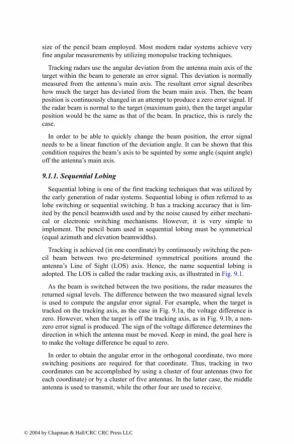
© 200
size of the pencil beam employed. Most modern radar systems achieve veryfine angular measurements by utilizing monopulse tracking techniques.
Tracking radars use the angular deviation from the antenna main axis of thetarget within the beam to generate an error signal. This deviation is normallymeasured from the antennas main axis. The resultant error signal describeshow much the target has deviated from the beam main axis. Then, the beamposition is continuously changed in an attempt to produce a zero error signal. Ifthe radar beam is normal to the target (maximum gain), then the target angularposition would be the same as that of the beam. In practice, this is rarely thecase.
In order to be able to quickly change the beam position, the error signalneeds to be a linear function of the deviation angle. It can be shown that thiscondition requires the beams axis to be squinted by some angle (squint angle)off the antennas main axis.
9.1.1. Sequential Lobing
Sequential lobing is one of the first tracking techniques that was utilized bythe early generation of radar systems. Sequential lobing is often referred to aslobe switching or sequential switching. It has a tracking accuracy that is lim-ited by the pencil beamwidth used and by the noise caused by either mechani-cal or electronic switching mechanisms. However, it is very simple toimplement. The pencil beam used in sequential lobing must be symmetrical(equal azimuth and elevation beamwidths).
Tracking is achieved (in one coordinate) by continuously switching the pen-cil beam between two pre-determined symmetrical positions around theantennas Line of Sight (LOS) axis. Hence, the name sequential lobing isadopted. The LOS is called the radar tracking axis, as illustrated in Fig. 9.1.
As the beam is switched between the two positions, the radar measures thereturned signal levels. The difference between the two measured signal levelsis used to compute the angular error signal. For example, when the target istracked on the tracking axis, as the case in Fig. 9.1a, the voltage difference iszero. However, when the target is off the tracking axis, as in Fig. 9.1b, a non-zero error signal is produced. The sign of the voltage difference determines thedirection in which the antenna must be moved. Keep in mind, the goal here isto make the voltage difference be equal to zero.
In order to obtain the angular error in the orthogonal coordinate, two moreswitching positions are required for that coordinate. Thus, tracking in twocoordinates can be accomplished by using a cluster of four antennas (two foreach coordinate) or by a cluster of five antennas. In the latter case, the middleantenna is used to transmit, while the other four are used to receive.
4 by Chapman & Hall/CRC CRC Press LLC
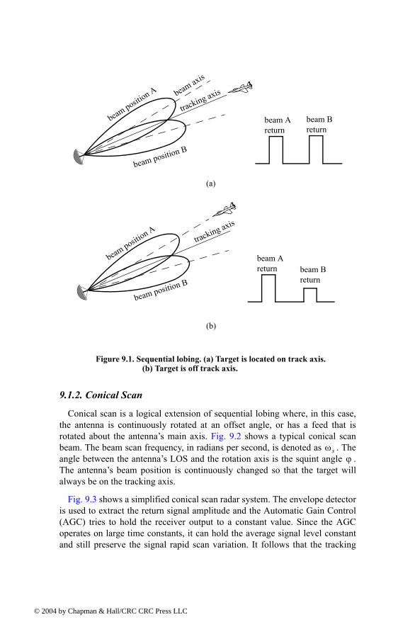
© 200
9.1.2. Conical Scan
Conical scan is a logical extension of sequential lobing where, in this case,the antenna is continuously rotated at an offset angle, or has a feed that isrotated about the antennas main axis. Fig. 9.2 shows a typical conical scanbeam. The beam scan frequency, in radians per second, is denoted as . Theangle between the antennas LOS and the rotation axis is the squint angle .The antennas beam position is continuously changed so that the target willalways be on the tracking axis.
Fig. 9.3 shows a simplified conical scan radar system. The envelope detectoris used to extract the return signal amplitude and the Automatic Gain Control(AGC) tries to hold the receiver output to a constant value. Since the AGCoperates on large time constants, it can hold the average signal level constantand still preserve the signal rapid scan variation. It follows that the tracking
beam axis
tracking axis
beam positi
on A
beam position B
beam Areturn beam B
return
(a)
beam position B
beam positi
on Atracking axis
beam Areturn
beam Breturn
(b)
Figure 9.1. Sequential lobing. (a) Target is located on track axis. (b) Target is off track axis.
ωsϕ
4 by Chapman & Hall/CRC CRC Press LLC
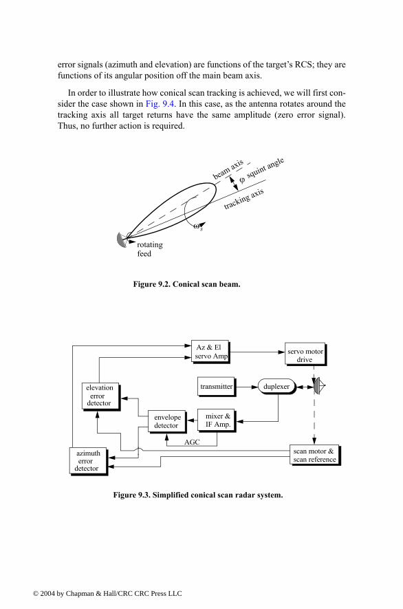
© 200
error signals (azimuth and elevation) are functions of the targets RCS; they arefunctions of its angular position off the main beam axis.
In order to illustrate how conical scan tracking is achieved, we will first con-sider the case shown in Fig. 9.4. In this case, as the antenna rotates around thetracking axis all target returns have the same amplitude (zero error signal).Thus, no further action is required.
tracking axis
beam axis
ϕ squint angle
rotatingfeed
Figure 9.2. Conical scan beam.
ωs
duplexertransmitter
mixer &IF Amp.
envelopedetector
AGCscan motor &scan reference
azimuth
detector error
elevation
detector error
Az & Elservo Amp servo motor
drive
Figure 9.3. Simplified conical scan radar system.
4 by Chapman & Hall/CRC CRC Press LLC
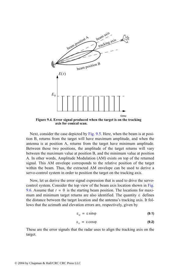
© 200
Next, consider the case depicted by Fig. 9.5. Here, when the beam is at posi-tion B, returns from the target will have maximum amplitude, and when theantenna is at position A, returns from the target have minimum amplitude.Between those two positions, the amplitude of the target returns will varybetween the maximum value at position B, and the minimum value at positionA. In other words, Amplitude Modulation (AM) exists on top of the returnedsignal. This AM envelope corresponds to the relative position of the targetwithin the beam. Thus, the extracted AM envelope can be used to derive aservo-control system in order to position the target on the tracking axis.
Now, let us derive the error signal expression that is used to drive the servo-control system. Consider the top view of the beam axis location shown in Fig.9.6. Assume that is the starting beam position. The locations for maxi-mum and minimum target returns are also identified. The quantity definesthe distance between the target location and the antennas tracking axis. It fol-lows that the azimuth and elevation errors are, respectively, given by
(9.1)
(9.2)
These are the error signals that the radar uses to align the tracking axis on thetarget.
beam axis
tracking axis
beam position A
beam position B
time
E t( )
E0
Figure 9.4. Error signal produced when the target is on the tracking axis for conical scan.
t 0=ε
εa ε ϕsin=
εe ε ϕcos=
4 by Chapman & Hall/CRC CRC Press LLC
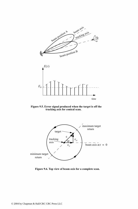
© 200
beam axis
tracking axis
beam positio
n A
beam position B
time
E t( )
E0
Figure 9.5. Error signal produced when the target is off the tracking axis for conical scan.
ϕ εa
εe
ε
beam axis at t 0=
maximum targetreturn
minimum targetreturn
trackingaxis
target
Figure 9.6. Top view of beam axis for a complete scan.
4 by Chapman & Hall/CRC CRC Press LLC
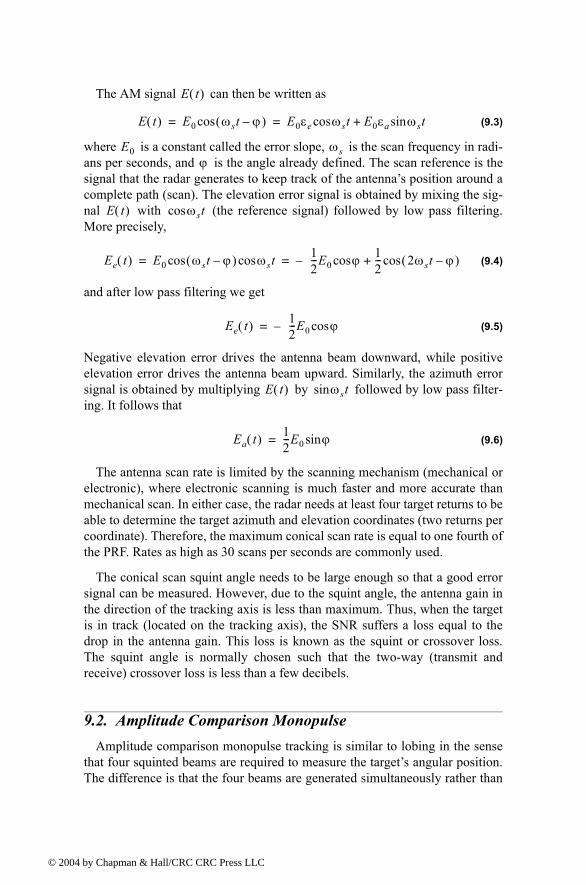
© 200
The AM signal can then be written as
(9.3)
where is a constant called the error slope, is the scan frequency in radi-ans per seconds, and is the angle already defined. The scan reference is thesignal that the radar generates to keep track of the antennas position around acomplete path (scan). The elevation error signal is obtained by mixing the sig-nal with (the reference signal) followed by low pass filtering.More precisely,
(9.4)
and after low pass filtering we get
(9.5)
Negative elevation error drives the antenna beam downward, while positiveelevation error drives the antenna beam upward. Similarly, the azimuth errorsignal is obtained by multiplying by followed by low pass filter-ing. It follows that
(9.6)
The antenna scan rate is limited by the scanning mechanism (mechanical orelectronic), where electronic scanning is much faster and more accurate thanmechanical scan. In either case, the radar needs at least four target returns to beable to determine the target azimuth and elevation coordinates (two returns percoordinate). Therefore, the maximum conical scan rate is equal to one fourth ofthe PRF. Rates as high as 30 scans per seconds are commonly used.
The conical scan squint angle needs to be large enough so that a good errorsignal can be measured. However, due to the squint angle, the antenna gain inthe direction of the tracking axis is less than maximum. Thus, when the targetis in track (located on the tracking axis), the SNR suffers a loss equal to thedrop in the antenna gain. This loss is known as the squint or crossover loss.The squint angle is normally chosen such that the two-way (transmit andreceive) crossover loss is less than a few decibels.
9.2. Amplitude Comparison MonopulseAmplitude comparison monopulse tracking is similar to lobing in the sense
that four squinted beams are required to measure the targets angular position.The difference is that the four beams are generated simultaneously rather than
E t( )
E t( ) E0 ωst ϕ( )cos E0εe ωstcos E0εa ωstsin+= =
E0 ωsϕ
E t( ) ωstcos
Ee t( ) E0 ωst ϕ( )cos ωstcos 12---E0 ϕcos 1
2--- 2ωst ϕ( )cos+= =
Ee t( ) 12---E0 ϕcos=
E t( ) ωssin t
Ea t( ) 12---E0 ϕsin=
4 by Chapman & Hall/CRC CRC Press LLC
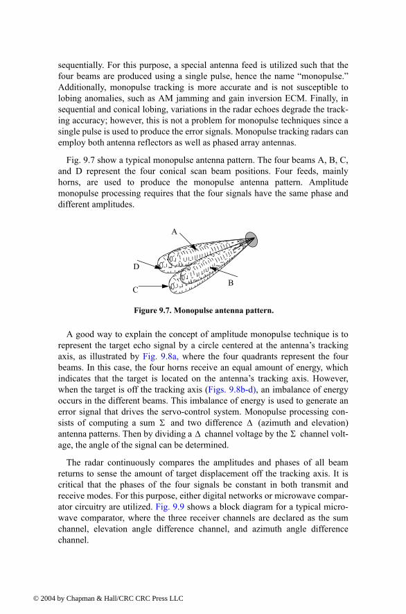
© 200
sequentially. For this purpose, a special antenna feed is utilized such that thefour beams are produced using a single pulse, hence the name monopulse.Additionally, monopulse tracking is more accurate and is not susceptible tolobing anomalies, such as AM jamming and gain inversion ECM. Finally, insequential and conical lobing, variations in the radar echoes degrade the track-ing accuracy; however, this is not a problem for monopulse techniques since asingle pulse is used to produce the error signals. Monopulse tracking radars canemploy both antenna reflectors as well as phased array antennas.
Fig. 9.7 show a typical monopulse antenna pattern. The four beams A, B, C,and D represent the four conical scan beam positions. Four feeds, mainlyhorns, are used to produce the monopulse antenna pattern. Amplitudemonopulse processing requires that the four signals have the same phase anddifferent amplitudes.
A good way to explain the concept of amplitude monopulse technique is torepresent the target echo signal by a circle centered at the antennas trackingaxis, as illustrated by Fig. 9.8a, where the four quadrants represent the fourbeams. In this case, the four horns receive an equal amount of energy, whichindicates that the target is located on the antennas tracking axis. However,when the target is off the tracking axis (Figs. 9.8b-d), an imbalance of energyoccurs in the different beams. This imbalance of energy is used to generate anerror signal that drives the servo-control system. Monopulse processing con-sists of computing a sum and two difference (azimuth and elevation)antenna patterns. Then by dividing a channel voltage by the channel volt-age, the angle of the signal can be determined.
The radar continuously compares the amplitudes and phases of all beamreturns to sense the amount of target displacement off the tracking axis. It iscritical that the phases of the four signals be constant in both transmit andreceive modes. For this purpose, either digital networks or microwave compar-ator circuitry are utilized. Fig. 9.9 shows a block diagram for a typical micro-wave comparator, where the three receiver channels are declared as the sumchannel, elevation angle difference channel, and azimuth angle differencechannel.
A
B
D
C
Figure 9.7. Monopulse antenna pattern.
Σ ∆∆ Σ
4 by Chapman & Hall/CRC CRC Press LLC
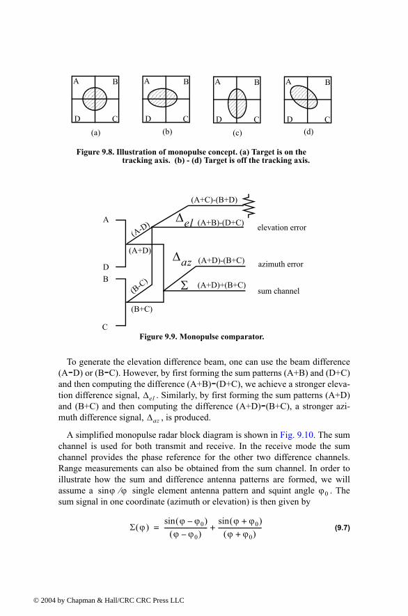
© 200
To generate the elevation difference beam, one can use the beam difference(A-D) or (B-C). However, by first forming the sum patterns (A+B) and (D+C)and then computing the difference (A+B)-(D+C), we achieve a stronger eleva-tion difference signal, . Similarly, by first forming the sum patterns (A+D)and (B+C) and then computing the difference (A+D)-(B+C), a stronger azi-muth difference signal, , is produced.
A simplified monopulse radar block diagram is shown in Fig. 9.10. The sumchannel is used for both transmit and receive. In the receive mode the sumchannel provides the phase reference for the other two difference channels.Range measurements can also be obtained from the sum channel. In order toillustrate how the sum and difference antenna patterns are formed, we willassume a single element antenna pattern and squint angle . Thesum signal in one coordinate (azimuth or elevation) is then given by
(9.7)
A B
D C
A B
D C
A B
D C
A B
D C(a) (b) (c) (d)
Figure 9.8. Illustration of monopulse concept. (a) Target is on the
tracking axis. (b) - (d) Target is off the tracking axis.
A
DB
C
(B-C)
(A-D)
(A+D)
(B+C)
∆az
∆el
Σ
(A+C)-(B+D)
(A+B)-(D+C)
(A+D)-(B+C)
(A+D)+(B+C)
elevation error
azimuth error
sum channel
Figure 9.9. Monopulse comparator.
∆el
∆az
ϕsin ϕ⁄ ϕ0
Σ ϕ( )ϕ ϕ0( )sin
ϕ ϕ0( )----------------------------
ϕ ϕ0+( )sinϕ ϕ0+( )
----------------------------+=
4 by Chapman & Hall/CRC CRC Press LLC
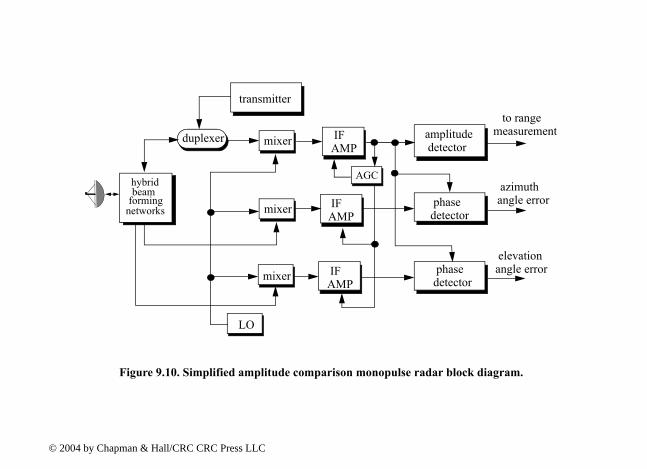
udetor
sector
etor
to rangemeasurement
azimuthangle error
elevationangle error
lock diagram.
hybridbeam
formingnetworks
transmitter
duplexer mixer
mixer
mixer
LO
IFAMP
IFAMP
IFAMP
amplit detec
phadete
phasdetec
Figure 9.10. Simplified amplitude comparison monopulse radar b
AGC
© 2004 by Chapman & Hall/CRC CRC Press LLC
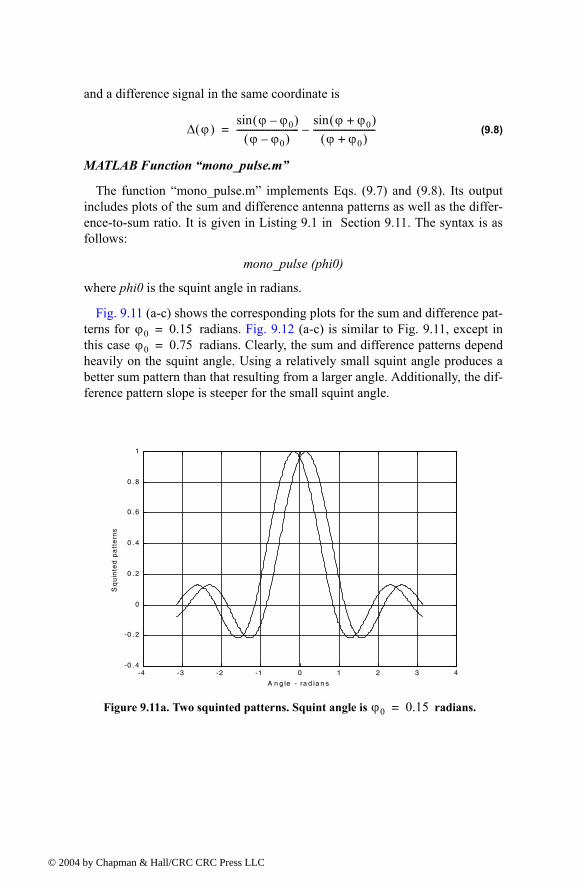
© 200
and a difference signal in the same coordinate is
(9.8)
MATLAB Function mono_pulse.m
The function mono_pulse.m implements Eqs. (9.7) and (9.8). Its outputincludes plots of the sum and difference antenna patterns as well as the differ-ence-to-sum ratio. It is given in Listing 9.1 in Section 9.11. The syntax is asfollows:
mono_pulse (phi0)
where phi0 is the squint angle in radians.
Fig. 9.11 (a-c) shows the corresponding plots for the sum and difference pat-terns for radians. Fig. 9.12 (a-c) is similar to Fig. 9.11, except inthis case radians. Clearly, the sum and difference patterns dependheavily on the squint angle. Using a relatively small squint angle produces abetter sum pattern than that resulting from a larger angle. Additionally, the dif-ference pattern slope is steeper for the small squint angle.
∆ ϕ( )ϕ ϕ0( )sin
ϕ ϕ0( )----------------------------
ϕ ϕ0+( )sinϕ ϕ0+( )
----------------------------=
ϕ0 0.15=ϕ0 0.75=
Figure 9.11a. Two squinted patterns. Squint angle is radians.ϕ0 0.15=
-4 -3 -2 -1 0 1 2 3 4-0 . 4
-0 . 2
0
0 . 2
0 . 4
0 . 6
0 . 8
1
A n g le - ra d ia n s
Sq
uin
ted
pa
tte
rns
4 by Chapman & Hall/CRC CRC Press LLC
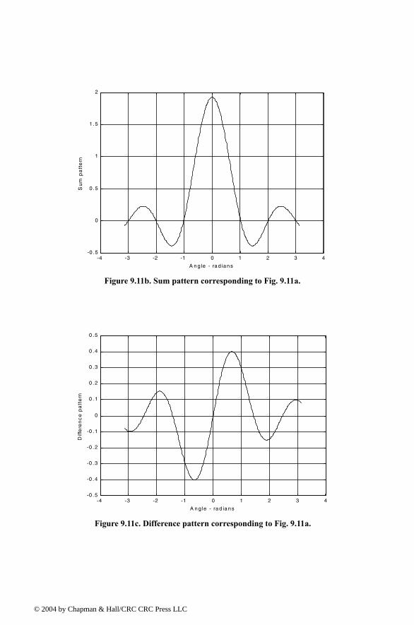
© 200
Figure 9.11b. Sum pattern corresponding to Fig. 9.11a.
-4 -3 -2 -1 0 1 2 3 4-0 .5
0
0 .5
1
1 .5
2
A n g le - ra d ia n s
Su
m p
att
ern
Figure 9.11c. Difference pattern corresponding to Fig. 9.11a.
-4 -3 -2 -1 0 1 2 3 4-0 .5
-0 .4
-0 .3
-0 .2
-0 .1
0
0 .1
0 .2
0 .3
0 .4
0 .5
A n g le - ra d ia n s
Diff
ere
nc
e p
att
ern
4 by Chapman & Hall/CRC CRC Press LLC
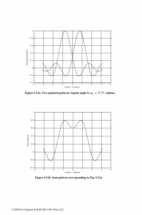
© 200
Figure 9.12a. Two squinted patterns. Squint angle is radians.ϕ0 0.75=
-4 -3 -2 -1 0 1 2 3 4-0 .4
-0 .2
0
0 .2
0 .4
0 .6
0 .8
1
A n g le - ra d ia n s
Sq
uin
ted
pa
tte
rns
Figure 9.12b. Sum pattern corresponding to Fig. 9.12a.
-4 -3 -2 -1 0 1 2 3 4-0 .4
-0 .2
0
0 .2
0 .4
0 .6
0 .8
1
A ng le - rad ians
Su
m p
att
ern
4 by Chapman & Hall/CRC CRC Press LLC
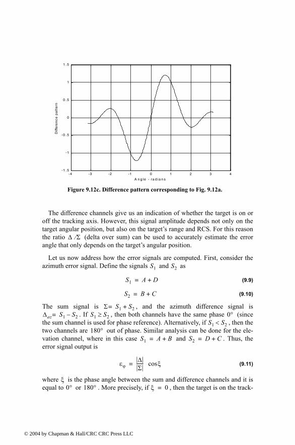
© 200
The difference channels give us an indication of whether the target is on oroff the tracking axis. However, this signal amplitude depends not only on thetarget angular position, but also on the targets range and RCS. For this reasonthe ratio (delta over sum) can be used to accurately estimate the errorangle that only depends on the targets angular position.
Let us now address how the error signals are computed. First, consider theazimuth error signal. Define the signals and as
(9.9)
(9.10)
The sum signal is , and the azimuth difference signal is. If , then both channels have the same phase (since
the sum channel is used for phase reference). Alternatively, if , then thetwo channels are out of phase. Similar analysis can be done for the ele-vation channel, where in this case and . Thus, theerror signal output is
(9.11)
where is the phase angle between the sum and difference channels and it isequal to or . More precisely, if , then the target is on the track-
Figure 9.12c. Difference pattern corresponding to Fig. 9.12a.
-4 -3 -2 -1 0 1 2 3 4-1 . 5
-1
-0 . 5
0
0 . 5
1
1 . 5
A n g le - ra d ia n s
Diff
ere
nc
e p
att
ern
∆ Σ⁄
S1 S2
S1 A D+=
S2 B C+=
Σ S1 S2+=∆az S1 S2= S1 S2≥ 0°
S1 S2<180°
S1 A B+= S2 D C+=
εϕ∆Σ
------ ξcos=
ξ0° 180° ξ 0=
4 by Chapman & Hall/CRC CRC Press LLC
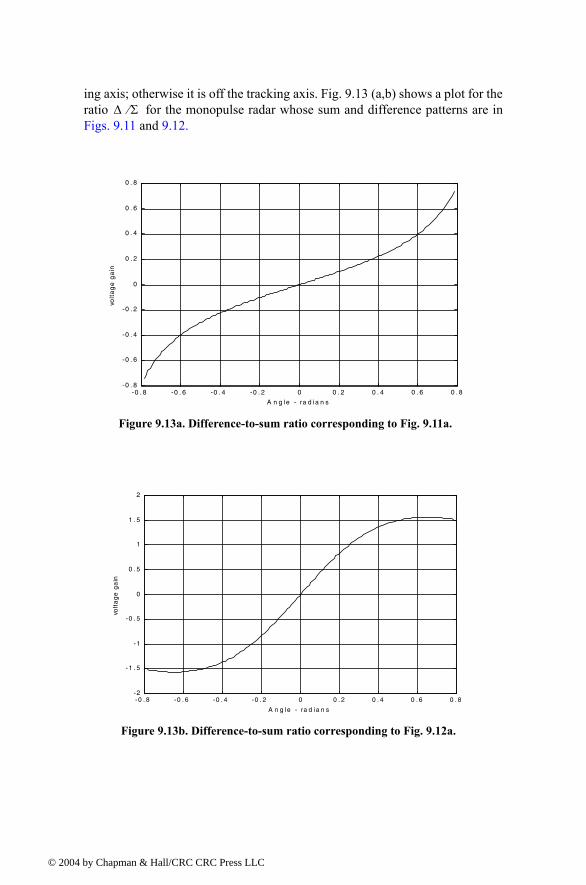
© 200
ing axis; otherwise it is off the tracking axis. Fig. 9.13 (a,b) shows a plot for theratio for the monopulse radar whose sum and difference patterns are inFigs. 9.11 and 9.12.
∆ Σ⁄
Figure 9.13a. Difference-to-sum ratio corresponding to Fig. 9.11a.
-0 . 8 -0 . 6 -0 . 4 -0 . 2 0 0 . 2 0 . 4 0 . 6 0 . 8-0 . 8
-0 . 6
-0 . 4
-0 . 2
0
0 . 2
0 . 4
0 . 6
0 . 8
A n g le - ra d ia n s
volt
ag
e g
ain
Figure 9.13b. Difference-to-sum ratio corresponding to Fig. 9.12a.
-0 . 8 -0 . 6 -0 . 4 -0 . 2 0 0 . 2 0 . 4 0 . 6 0 . 8-2
-1 . 5
-1
-0 . 5
0
0 . 5
1
1 . 5
2
A n g le - ra d ia n s
volt
ag
e g
ain
4 by Chapman & Hall/CRC CRC Press LLC
© 200
9.3. Phase Comparison MonopulsePhase comparison monopulse is similar to amplitude comparison monopulse
in the sense that the target angular coordinates are extracted from one sum andtwo difference channels. The main difference is that the four signals producedin amplitude comparison monopulse will have similar phases but differentamplitudes; however, in phase comparison monopulse the signals have thesame amplitude and different phases. Phase comparison monopulse trackingradars use a minimum of a two-element array antenna for each coordinate (azi-muth and elevation), as illustrated in Fig. 9.14. A phase error signal (for eachcoordinate) is computed from the phase difference between the signals gener-ated in the antenna elements.
Consider Fig. 9.14; since the angle is equal to , it follows that
(9.12)
and since we can use the binomial series expansion to get
(9.13)
R1
RR2
ϕα
d
antenna axis
target
Figure 9.14. Single coordinate phase comparison monopulse antenna.
α ϕ π 2⁄+
R12 R2 d
2---
22d
2---R ϕ π
2---+
cos+
R2 d4---
2dR ϕsin+
=
=
d R«
R1 R 1 d2R------- ϕsin+
≈
4 by Chapman & Hall/CRC CRC Press LLC
© 200
Similarly,
(9.14)
The phase difference between the two elements is then given by
(9.15)
where is the wavelength. The phase difference is used to determine theangular target location. Note that if , then the target would be on theantennas main axis. The problem with this phase comparison monopulse tech-nique is that it is quite difficult to maintain a stable measurement of the offboresight angle , which causes serious performance degradation. This prob-lem can be overcome by implementing a phase comparison monopulse systemas illustrated in Fig. 9.15.
The (single coordinate) sum and difference signals are, respectively, givenby
(9.16)
(9.17)
where the and are the signals in the two elements. Now, since and have similar amplitude and are different in phase by , we can write
(9.18)
It follows that
(9.19)
R2 R 1 d2R------- ϕsin
≈
φ 2πλ
------ R1 R2( ) 2πλ
------d ϕsin= =
λ φφ 0=
ϕ
Σ ϕ( ) S1 S2+=
∆ ϕ( ) S1 S2=
S1 S2 S1S2 φ
S1 S2e jφ=
∆ ϕ( ) S2 1 e jφ( )=
ϕ dΣ
∆
Figure 9.15. Single coordinate phase monopulse antenna, with sum and difference channels.
S2
S1
4 by Chapman & Hall/CRC CRC Press LLC
© 200
(9.20)
The phase error signal is computed from the ratio . More precisely,
(9.21)
which is purely imaginary. The modulus of the error signal is then given by
(9.22)
This kind of phase comparison monopulse tracker is often called the half-angletracker.
9.4. Range TrackingTarget range is measured by estimating the round-trip delay of the transmit-
ted pulses. The process of continuously estimating the range of a moving targetis known as range tracking. Since the range to a moving target is changing withtime, the range tracker must be constantly adjusted to keep the target locked inrange. This can be accomplished using a split gate system, where two rangegates (early and late) are utilized. The concept of split gate tracking is illus-trated in Fig. 9.16, where a sketch of a typical pulsed radar echo is shown in thefigure. The early gate opens at the anticipated starting time of the radar echoand lasts for half its duration. The late gate opens at the center and closes at theend of the echo signal. For this purpose, good estimates of the echo durationand the pulse center time must be reported to the range tracker so that the earlyand late gates can be placed properly at the start and center times of theexpected echo. This reporting process is widely known as the designation pro-cess.
The early gate produces positive voltage output while the late gate producesnegative voltage output. The outputs of the early and late gates are subtracted,and the difference signal is fed into an integrator to generate an error signal. Ifboth gates are placed properly in time, the integrator output will be equal tozero. Alternatively, when the gates are not timed properly, the integrator outputis not zero, which gives an indication that the gates must be moved in time, leftor right depending on the sign of the integrator output.
Σ ϕ( ) S2 1 e jφ+( )=
∆ Σ⁄
∆Σ--- 1 e jφ
1 e jφ+------------------ j φ
2--- tan= =
∆Σ
------ φ2--- tan=
4 by Chapman & Hall/CRC CRC Press LLC
© 200
radar echo
early gate
late gate
early gate response
late gate response
Figure 9.16. Illustration of split-range gate.
4 by Chapman & Hall/CRC CRC Press LLC
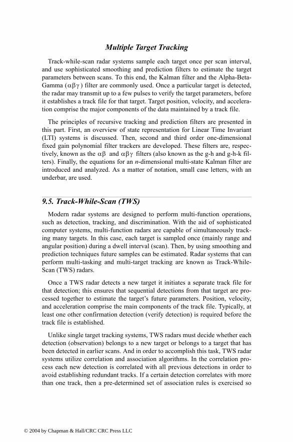
© 200
Multiple Target Tracking
Track-while-scan radar systems sample each target once per scan interval,and use sophisticated smoothing and prediction filters to estimate the targetparameters between scans. To this end, the Kalman filter and the Alpha-Beta-Gamma ( ) filter are commonly used. Once a particular target is detected,the radar may transmit up to a few pulses to verify the target parameters, beforeit establishes a track file for that target. Target position, velocity, and accelera-tion comprise the major components of the data maintained by a track file.
The principles of recursive tracking and prediction filters are presented inthis part. First, an overview of state representation for Linear Time Invariant(LTI) systems is discussed. Then, second and third order one-dimensionalfixed gain polynomial filter trackers are developed. These filters are, respec-tively, known as the and filters (also known as the g-h and g-h-k fil-ters). Finally, the equations for an n-dimensional multi-state Kalman filter areintroduced and analyzed. As a matter of notation, small case letters, with anunderbar, are used.
9.5. Track-While-Scan (TWS)Modern radar systems are designed to perform multi-function operations,
such as detection, tracking, and discrimination. With the aid of sophisticatedcomputer systems, multi-function radars are capable of simultaneously track-ing many targets. In this case, each target is sampled once (mainly range andangular position) during a dwell interval (scan). Then, by using smoothing andprediction techniques future samples can be estimated. Radar systems that canperform multi-tasking and multi-target tracking are known as Track-While-Scan (TWS) radars.
Once a TWS radar detects a new target it initiates a separate track file forthat detection; this ensures that sequential detections from that target are pro-cessed together to estimate the targets future parameters. Position, velocity,and acceleration comprise the main components of the track file. Typically, atleast one other confirmation detection (verify detection) is required before thetrack file is established.
Unlike single target tracking systems, TWS radars must decide whether eachdetection (observation) belongs to a new target or belongs to a target that hasbeen detected in earlier scans. And in order to accomplish this task, TWS radarsystems utilize correlation and association algorithms. In the correlation pro-cess each new detection is correlated with all previous detections in order toavoid establishing redundant tracks. If a certain detection correlates with morethan one track, then a pre-determined set of association rules is exercised so
αβγ
αβ αβγ
4 by Chapman & Hall/CRC CRC Press LLC
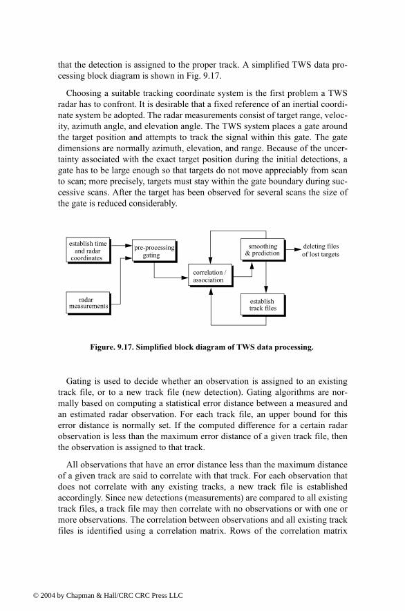
© 200
that the detection is assigned to the proper track. A simplified TWS data pro-cessing block diagram is shown in Fig. 9.17.
Choosing a suitable tracking coordinate system is the first problem a TWSradar has to confront. It is desirable that a fixed reference of an inertial coordi-nate system be adopted. The radar measurements consist of target range, veloc-ity, azimuth angle, and elevation angle. The TWS system places a gate aroundthe target position and attempts to track the signal within this gate. The gatedimensions are normally azimuth, elevation, and range. Because of the uncer-tainty associated with the exact target position during the initial detections, agate has to be large enough so that targets do not move appreciably from scanto scan; more precisely, targets must stay within the gate boundary during suc-cessive scans. After the target has been observed for several scans the size ofthe gate is reduced considerably.
Gating is used to decide whether an observation is assigned to an existingtrack file, or to a new track file (new detection). Gating algorithms are nor-mally based on computing a statistical error distance between a measured andan estimated radar observation. For each track file, an upper bound for thiserror distance is normally set. If the computed difference for a certain radarobservation is less than the maximum error distance of a given track file, thenthe observation is assigned to that track.
All observations that have an error distance less than the maximum distanceof a given track are said to correlate with that track. For each observation thatdoes not correlate with any existing tracks, a new track file is establishedaccordingly. Since new detections (measurements) are compared to all existingtrack files, a track file may then correlate with no observations or with one ormore observations. The correlation between observations and all existing trackfiles is identified using a correlation matrix. Rows of the correlation matrix
establish timeand radar
coordinates
radarmeasurements
pre-processing gating
correlation /association
smoothing& prediction
establishtrack files
deleting filesof lost targets
Figure. 9.17. Simplified block diagram of TWS data processing.
4 by Chapman & Hall/CRC CRC Press LLC
© 200
represent radar observations, while columns represent track files. In caseswhere several observations correlate with more than one track file, a set of pre-determined association rules can be utilized so that a single observation isassigned to a single track file.
9.6. State Variable Representation of an LTI System A linear time invariant system (continuous or discrete) can be described
mathematically using three variables. They are the input, output, and the statevariables. In this representation, any LTI system has observable or measurableobjects (abstracts). For example, in the case of a radar system, range may be anobject measured or observed by the radar tracking filter. States can be derivedin many different ways. For the scope of this book, states of an object or anabstract are the components of the vector that contains the object and its timederivatives. For example, a third-order one-dimensional (in this case range)state vector representing range can be given by
(9.23)
where , , and are, respectively, the range measurement, range rate(velocity), and acceleration. The state vector defined in Eq. (9.23) can be rep-resentative of continuous or discrete states. In this book, the emphasis is ondiscrete time representation, since most radar signal processing is executedusing digital computers. For this purpose, an n-dimensional state vector has thefollowing form:
(9.24)
where the superscript indicates the transpose operation.
The LTI system of interest can be represented using the following state equa-tions:
(9.25)
(9.26)
where: is the value of the state vector; is the value of the out-put vector; is the value of the input vector; is an matrix; is an matrix; is matrix; and is an matrix. The
xRR·
R··=
R R· R··
x x1 x· 1 … x2 x·2 … xn x·n …t
=
x· t( ) A x t( ) Bw t( )+=
y t( ) C x t( ) Dw t( )+=
x· n 1× y p 1×w m 1× A n n× B
n m× C p n× D p m×
4 by Chapman & Hall/CRC CRC Press LLC
© 200
homogeneous solution (i.e., ) to this linear system, assuming knowninitial condition at time , has the form
(9.27)
The matrix is known as the state transition matrix, or fundamental matrix,and is equal to
(9.28)
Eq. (9.28) can be expressed in series format as
(9.29)
Example:
Compute the state transition matrix for an LTI system when
Solution:
The state transition matrix can be computed using Eq. (9.29). For this pur-pose, compute and . It follows
Therefore,
The state transition matrix has the following properties (the proof is left asan exercise):
1. Derivative property
w 0=x 0( ) t0
x t( ) Φ t t0( )x t t0( )=
Φ
Φ t t0( ) eA t t0( )
=
Φ t t0( )t0 0=
eA t( ) I At A2 t2
2!----- …+ + + Ak tk
k!----
k 0=
∞
∑= = =
A 0 10.5 1
=
A2 A3…
A212--- 1
12--- 1
2---
= A312--- 1
2---
14--- 0
= …
Φ1 0t
12---t2
2!-------
12---t3
3!------- …+ ++ 0 t t2
2!-----
12--- t3
3!------- …+ ++
0 12---t
12---t2
2!-------+
14---t3
3!------- …+ 1 t
12---t2
2!------- 0t3
3!------- …+ + +
=
4 by Chapman & Hall/CRC CRC Press LLC
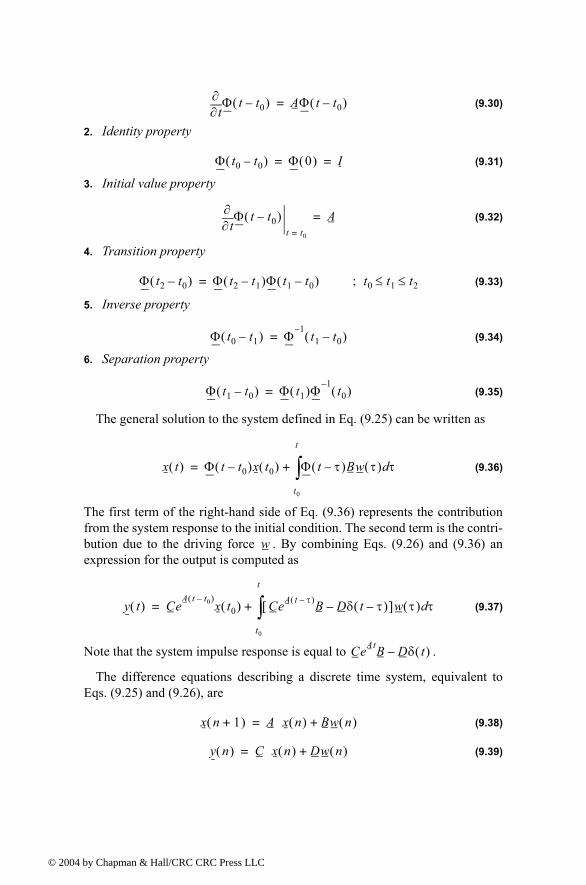
© 200
(9.30)
2. Identity property
(9.31)
3. Initial value property
(9.32)
4. Transition property
(9.33)
5. Inverse property
(9.34)
6. Separation property
(9.35)
The general solution to the system defined in Eq. (9.25) can be written as
(9.36)
The first term of the right-hand side of Eq. (9.36) represents the contributionfrom the system response to the initial condition. The second term is the contri-bution due to the driving force . By combining Eqs. (9.26) and (9.36) anexpression for the output is computed as
(9.37)
Note that the system impulse response is equal to .
The difference equations describing a discrete time system, equivalent toEqs. (9.25) and (9.26), are
(9.38)
(9.39)
t∂∂ Φ t t0( ) AΦ t t0( )=
Φ t0 t0( ) Φ 0( ) I= =
t∂∂ Φ t t0( )
t t0=
A=
Φ t2 t0( ) Φ t2 t1( )Φ t1 t0( )= t0 t1 t2≤ ≤;
Φ t0 t1( ) Φ1
t1 t0( )=
Φ t1 t0( ) Φ t1( )Φ1
t0( )=
x t( ) Φ t t0( )x t0( ) Φ t τ( )Bw τ( ) τd
t0
t
∫+=
w
y t( ) CeA t t0( )
x t0( ) CeA t τ( )B Dδ t τ( )[ ]w τ( ) τd
t0
t
∫+=
CeAtB Dδ t( )
x n 1+( ) A x n( ) Bw n( )+=
y n( ) C x n( ) Dw n( )+=
4 by Chapman & Hall/CRC CRC Press LLC

© 200
where defines the discrete time and is the sampling interval. All othervectors and matrices were defined earlier. The homogeneous solution to thesystem defined in Eq. (9.38), with initial condition , is
(9.40)
In this case the state transition matrix is an matrix given by
(9.41)
The following is the list of properties associated with the discrete transitionmatrix
(9.42)
(9.43)
(9.44)
(9.45)
(9.46)
(9.47)
The solution to the general case (i.e., non-homogeneous system) is given by
(9.48)
It follows that the output is given by
(9.49)
where the system impulse response is given by
(9.50)
Taking the Z-transform for Eqs. (9.38) and (9.39) yields
n nT T
x n0( )
x n( ) An n0
x n0( )=
n n×
Φ n n0,( ) Φ n n0( ) An n0
= =
Φ n 1 n0+( ) AΦ n n0( )=
Φ n0 n0( ) Φ 0( ) I= =
Φ n0 1 n0+( ) Φ 1( ) A= =
Φ n2 n0( ) Φ n2 n1( )Φ n1 n0( )=
Φ n0 n1( ) Φ1
n1 n0( )=
Φ n1 n0( ) Φ n1( )Φ1
n0( )=
x n( ) Φ n n0( )x n0( ) Φ n m 1( )Bw m( )
m n0=
n 1
∑+=
y n( ) CΦ n n0( )x n0( ) C Φ n m 1( )Bw m( ) Dw n( )+
m n0=
n 1
∑+=
h n( ) C Φ n m 1( )Bδ m( ) Dδ n( )+
m n0=
n 1
∑=
4 by Chapman & Hall/CRC CRC Press LLC
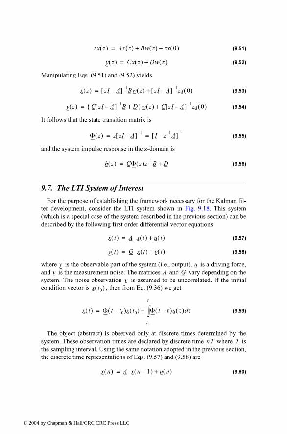
© 200
(9.51)
(9.52)
Manipulating Eqs. (9.51) and (9.52) yields
(9.53)
(9.54)
It follows that the state transition matrix is
(9.55)
and the system impulse response in the z-domain is
(9.56)
9.7. The LTI System of Interest For the purpose of establishing the framework necessary for the Kalman fil-
ter development, consider the LTI system shown in Fig. 9.18. This system(which is a special case of the system described in the previous section) can bedescribed by the following first order differential vector equations
(9.57)
(9.58)
where is the observable part of the system (i.e., output), is a driving force,and is the measurement noise. The matrices and vary depending on thesystem. The noise observation is assumed to be uncorrelated. If the initialcondition vector is , then from Eq. (9.36) we get
(9.59)
The object (abstract) is observed only at discrete times determined by thesystem. These observation times are declared by discrete time where isthe sampling interval. Using the same notation adopted in the previous section,the discrete time representations of Eqs. (9.57) and (9.58) are
(9.60)
zx z( ) Ax z( ) Bw z( ) zx 0( )+ +=
y z( ) Cx z( ) Dw z( )+=
x z( ) zI A[ ] 1 Bw z( ) zI A[ ] 1 zx 0( )+=
y z( ) C zI A[ ] 1 B D+ w z( ) C zI A[ ] 1 zx 0( )+=
Φ z( ) z zI A[ ] 1 I z 1 A[ ]1
= =
h z( ) CΦ z( )z 1 B D+=
x· t( ) A x t( ) u t( )+=
y t( ) G x t( ) v t( )+=
y uv A G
vx t0( )
x t( ) Φ t t0( )x t0( ) Φ t τ( )u τ( ) τd
t0
t
∫+=
nT T
x n( ) A x n 1( ) u n( )+=
4 by Chapman & Hall/CRC CRC Press LLC
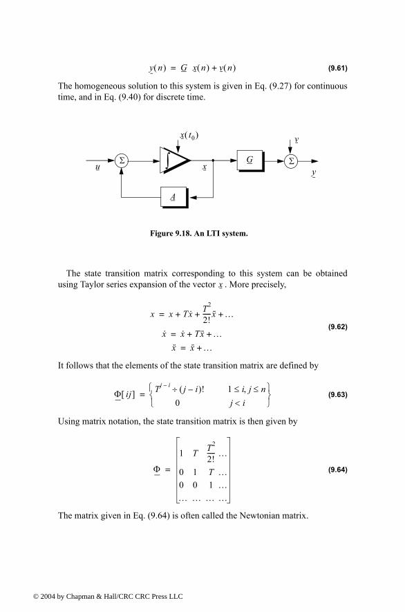
© 200
(9.61)
The homogeneous solution to this system is given in Eq. (9.27) for continuoustime, and in Eq. (9.40) for discrete time.
The state transition matrix corresponding to this system can be obtainedusing Taylor series expansion of the vector . More precisely,
(9.62)
It follows that the elements of the state transition matrix are defined by
(9.63)
Using matrix notation, the state transition matrix is then given by
(9.64)
The matrix given in Eq. (9.64) is often called the Newtonian matrix.
y n( ) G x n( ) v n( )+=
Σ Σu
A
∫ Gy
x t0( )
x
v
Figure 9.18. An LTI system.
x
x x Tx· T2
2!-----x·· …+ + +=
x· x· Tx·· …+ +=
x·· x·· …+=
Φ ij[ ] Tj i j i( )!÷ 1 i j n≤,≤0 j i<
=
Φ
1 T T2
2!----- …
0 1 T …0 0 1 …… … … …
=
4 by Chapman & Hall/CRC CRC Press LLC
© 200
9.8. Fixed-Gain Tracking Filters This class of filters (or estimators) is also known as Fixed-Coefficient fil-
ters. The most common examples of this class of filters are the and filters and their variations. The and trackers are one-dimensional sec-ond and third order filters, respectively. They are equivalent to special cases ofthe one-dimensional Kalman filter. The general structure of this class of esti-mators is similar to that of the Kalman filter.
The standard filter provides smoothed and predicted data for targetposition, velocity (Doppler), and acceleration. It is a polynomial predictor/cor-rector linear recursive filter. This filter can reconstruct position, velocity, andconstant acceleration based on position measurements. The filter can alsoprovide a smoothed (corrected) estimate of the present position which can beused in guidance and fire control operations.
Notation:
For the purpose of the discussion presented in the remainder of this chapter,the following notation is adopted: represents the estimate during the
sampling interval, using all data up to and including the samplinginterval; is the measured value; and is the residual (error).
The fixed-gain filter equation is given by
(9.65)
Since the transition matrix assists in predicting the next state,
(9.66)
Substituting Eq. (9.66) into Eq. (9.65) yields
(9.67)
The term enclosed within the brackets on the right hand side of Eq. (9.67) isoften called the residual (error) which is the difference between the measuredinput and predicted output. Eq. (9.67) means that the estimate of is thesum of the prediction and the weighted residual. The term repre-sents the prediction state. In the case of the estimator, is the row vectorgiven by
(9.68)
and the gain matrix is given by
αβ αβγαβ αβγ
αβγ
αβγ
x n m( )nth mth
yn nth en nth
x n n( ) Φx n 1 n 1( ) K yn GΦx n 1 n 1( )[ ]+=
x n 1+ n( ) Φx n n( )=
x n n( ) x n n 1( ) K yn Gx n n 1( )[ ]+=
x n( )Gx n n 1( )
αβγ G
G 1 0 0 …=
K
4 by Chapman & Hall/CRC CRC Press LLC
© 200
(9.69)
One of the main objectives of a tracking filter is to decrease the effect of thenoise observation on the measurement. For this purpose the noise covariancematrix is calculated. More precisely, the noise covariance matrix is
(9.70)
where indicates the expected value operator. Noise is assumed to be a zeromean random process with variance equal to . Additionally, noise measure-ments are also assumed to be uncorrelated,
(9.71)
Eq. (9.65) can be written as
(9.72)
where
(9.73)
Substituting Eqs. (9.72) and (9.73) into Eq. (9.70) yields
(9.74)
Expanding the right hand side of Eq. (9.74) and using Eq. (9.71) give
(9.75)
Under the steady state condition, Eq. (9.75) collapses to
(9.76)
where is the steady state noise covariance matrix. In the steady state,
(9.77)
Several criteria can be used to establish the performance of the fixed-gaintracking filter. The most commonly used technique is to compute the VarianceReduction Ratio (VRR). The VRR is defined only when the input to the trackeris noise measurements. It follows that in the steady state case, the VRR is the
Kαβ T⁄
γ T2⁄
=
C n n( ) E x n n( )( )xt n n( ) = yn; vn=
Eσv
2
E vnvm δσv
2 n m=
0 n m≠
=
x n n( ) Ax n 1 n 1( ) Kyn+=
A I KG( )Φ=
C n n( ) E Ax n 1 n 1( ) Kyn+( ) Ax n 1 n 1( ) Kyn+( )t =
C n n( ) AC n 1 n 1( )At Kσv2Kt+=
C n n( ) ACAt Kσv2Kt+=
C
C n n( ) C n 1 n 1( ) C= = for any n
4 by Chapman & Hall/CRC CRC Press LLC
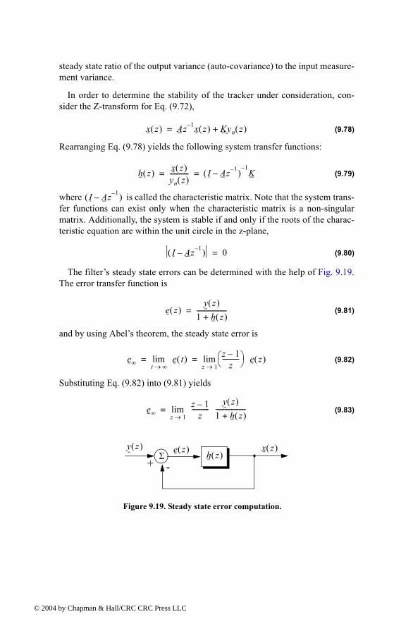
© 200
steady state ratio of the output variance (auto-covariance) to the input measure-ment variance.
In order to determine the stability of the tracker under consideration, con-sider the Z-transform for Eq. (9.72),
(9.78)
Rearranging Eq. (9.78) yields the following system transfer functions:
(9.79)
where is called the characteristic matrix. Note that the system trans-fer functions can exist only when the characteristic matrix is a non-singularmatrix. Additionally, the system is stable if and only if the roots of the charac-teristic equation are within the unit circle in the z-plane,
(9.80)
The filters steady state errors can be determined with the help of Fig. 9.19.The error transfer function is
(9.81)
and by using Abels theorem, the steady state error is
(9.82)
Substituting Eq. (9.82) into (9.81) yields
(9.83)
x z( ) Az 1 x z( ) Kyn z( )+=
h z( ) x z( )yn z( )------------ I Az 1( )
1K= =
I Az 1( )
I Az 1( ) 0=
e z( )y z( )
1 h z( )+-------------------=
e∞ e t( )t ∞→lim z 1
z----------- e z( )
z 1→lim= =
e∞z 1
z-----------
y z( )1 h z( )+-------------------
z 1→lim=
Σy z( ) x z( )
h z( )e z( )+ -
Figure 9.19. Steady state error computation.
4 by Chapman & Hall/CRC CRC Press LLC
© 200
9.8.1. The Filter
The tracker produces, on the observation, smoothed estimates forposition and velocity, and a predicted position for the observation.Fig. 9.20 shows an implementation of this filter. Note that the subscripts pand s are used to indicate, respectively, the predicated and smoothed values.The tracker can follow an input ramp (constant velocity) with no steadystate errors. However, a steady state error will accumulate when constantacceleration is present in the input. Smoothing is done to reduce errors in thepredicted position through adding a weighted difference between the measuredand predicted values to the predicted position, as follows:
(9.84)
(9.85)
is the position input samples. The predicted position is given by
(9.86)
The initialization process is defined by
A general form for the covariance matrix was developed in the previous sec-tion, and is given in Eq. (9.75). In general, a second order one-dimensionalcovariance matrix (in the context of the filter) can be written as
(9.87)
where, in general, is
(9.88)
By inspection, the filter has
(9.89)
αβαβ nth
n 1+( )th
αβ
xs n( ) x n n( ) xp n( ) α x0 n( ) xp n( )( )+= =
x· s n( ) x' n n( ) x· s n 1( ) βT--- x0 n( ) xp n( )( )+= =
x0
xp n( ) xs n n 1( ) xs n 1( ) Tx· s n 1( )+= =
xs 1( ) xp 2( ) x0 1( )= =
x· s 1( ) 0=
x· s 2( )x0 2( ) x0 1( )
T--------------------------------=
αβ
C n n( )Cxx Cxx·
Cx· x Cx· x·=
Cxy
Cxy E xyt =
αβ
A 1 α 1 α( )Tβ T⁄ 1 β( )
=
4 by Chapman & Hall/CRC CRC Press LLC
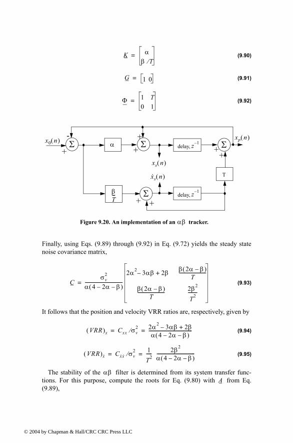
© 200
(9.90)
(9.91)
(9.92)
Finally, using Eqs. (9.89) through (9.92) in Eq. (9.72) yields the steady statenoise covariance matrix,
(9.93)
It follows that the position and velocity VRR ratios are, respectively, given by
(9.94)
(9.95)
The stability of the filter is determined from its system transfer func-tions. For this purpose, compute the roots for Eq. (9.80) with from Eq.(9.89),
K αβ T⁄
=
G 1 0=
Φ 1 T0 1
=
Σ
Σ Σ Σ
delay, z 1
delay, z 1
T
α
βT---
-
+ ++
++
++
xp n( )
x· s n( )
xs n( )
x0 n( )
Figure 9.20. An implementation of an tracker.αβ
Cσv
2
α 4 2α β( )----------------------------------
2α2 3αβ 2β+β 2α β( )
T------------------------
β 2α β( )T
------------------------ 2β2
T2--------
=
VRR( )x Cxx σv2⁄ 2α2 3αβ 2β+
α 4 2α β( )---------------------------------------= =
VRR( )x· Cx· x· σv2⁄ 1
T2----- 2β2
α 4 2α β( )----------------------------------= =
αβA
4 by Chapman & Hall/CRC CRC Press LLC
© 200
(9.96)
Solving Eq. (9.96) for yields
(9.97)
and in order to guarantee stability
(9.98)
Two cases are analyzed. First, are real. In this case (the details are left asan exercise),
(9.99)The second case is when the roots are complex; in this case we find
(9.100)
The system transfer functions can be derived by using Eqs. (9.79), (9.89),and (9.90),
(9.101)
Up to this point all relevant relations concerning the filter were madewith no regard to how to choose the gain coefficients ( and ). Before con-sidering the methodology of selecting these coefficients, consider the mainobjective behind using this filter. The twofold purpose of the tracker canbe described as follows:
1. The tracker must reduce the measurement noise as much as possible.2. The filter must be able to track maneuvering targets, with as little residual
(tracking error) as possible.
The reduction of measurement noise is normally determined by the VRRratios. However, the maneuverability performance of the filter depends heavilyon the choice of the parameters and .
A special variation of the filter was developed by Benedict and Bord-ner1, and is often referred to as the Benedict-Bordner filter. The main advan-
1. Benedict, T. R. and Bordner, G. W., Synthesis of an Optimal Set of Radar Track-While-Scan Smoothing Equations, IRE Transaction on Automatic Control, AC-7, July 1962, pp. 27-32.
I Az 1 1 2 α β( )z 1 1 α( )z 2+ 0= =
z
z1 2, 1 α β+2
------------- 12--- α β( )2 4β±=
z1 2, 1<
z1 2,
β 0> α β>;
α 0>
hx z( )hx· z( )
1z2 z 2 α β( ) 1 α( )+----------------------------------------------------------------
αz z α β( )α
-----------------
βz z 1( )T
----------------------=
αβα β
αβ
α β
αβ
4 by Chapman & Hall/CRC CRC Press LLC
© 200
tage of the Benedict-Bordner is reducing the transient errors associated withthe tracker. This filter uses both the position and velocity VRR ratios asmeasures of performance. It computes the sum of the squared differencesbetween the input (position) and the output when the input has a unit stepvelocity at time zero. Additionally, it computes the squared differencesbetween the real velocity and the velocity output when the input is as describedearlier. Both error differences are minimized when
(9.102)
In this case, the position and velocity VRR ratios are, respectively, given by
(9.103)
(9.104)
Another important sub-class of the tracker is the critically damped filter,often called the fading memory filter. In this case, the filter coefficients arechosen on the basis of a smoothing factor , where . The gain coeffi-cients are given by
(9.105)
(9.106)
Heavy smoothing means and little smoothing means . The ele-ments of the covariance matrix for a fading memory filter are
(9.107)
(9.108)
(9.109)
9.8.2. The Filter
The tracker produces, for the observation, smoothed estimates ofposition, velocity, and acceleration. It also produces the predicted position and
αβ
β α2
2 α------------=
VRR( )xα 6 5α( )
α2 8α 8+----------------------------=
VRR( )x·2T2----- α3 2 α( )⁄
α2 8α 8+----------------------------=
αβ
ξ 0 ξ 1≤ ≤
α 1 ξ2=
β 1 ξ( )2=
ξ 1→ ξ 0→
Cxx1 ξ
1 ξ+( )3------------------- 1 4ξ 5ξ2+ +( ) σv
2=
Cxx· Cx· x1T--- 1 ξ
1 ξ+( )3------------------- 1 2ξ 3ξ2+ +( ) σv
2= =
Cx· x·2T2----- 1 ξ
1 ξ+( )3------------------- 1 ξ( )2 σv
2=
αβγαβγ nth
4 by Chapman & Hall/CRC CRC Press LLC
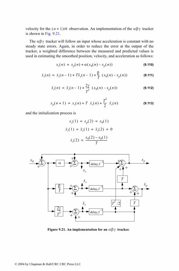
© 200
velocity for the observation. An implementation of the trackeris shown in Fig. 9.21.
The tracker will follow an input whose acceleration is constant with nosteady state errors. Again, in order to reduce the error at the output of thetracker, a weighted difference between the measured and predicted values isused in estimating the smoothed position, velocity, and acceleration as follows:
(9.110)
(9.111)
(9.112)
(9.113)
and the initialization process is
n 1+( )th αβγ
αβγ
xs n( ) xp n( ) α x0 n( ) xp n( )( )+=
x· s n( ) x· s n 1( ) Tx··s n 1( ) βT--- x0 n( ) xp n( )( )+ +=
x··s n( ) x··s n 1( ) 2γT2----- x0 n( ) xp n( )( )+=
xp n 1+( ) xs n( ) T x· s n( ) T2
2----- x··s n( )+ +=
xs 1( ) xp 2( ) x0 1( )= =
x· s 1( ) x··s 1( ) x··s 2( ) 0= = =
x· s 2( )x0 2( ) x0 1( )
T--------------------------------=
Σ
Σ Σ Σdelay, z 1α
βT---
-+
+ xp
x·px· s
xs
x0
Figure 9.21. An implementation for an tracker.αβγ
Σ
2γT2-----
T
T2 2⁄ T
Σ
x··s
delay, z 1
delay, z 1
+++
++ +
+
+
++
4 by Chapman & Hall/CRC CRC Press LLC
© 200
Using Eq. (9.63) the state transition matrix for the filter is
(9.114)
The covariance matrix (which is symmetric) can be computed from Eq. (9.76).For this purpose, note that
(9.115)
(9.116)
and
(9.117)
Substituting Eq. (9.117) into (9.76) and collecting terms the VRR ratios arecomputed as
(9.118)
(9.119)
(9.120)
As in the case of any discrete time system, this filter will be stable if and only ifall of its poles fall within the unit circle in the z-plane.
The characteristic equation is computed by setting
x··s 3( )x0 3( ) x0 1( ) 2x0 2( )+
T2-------------------------------------------------------=
αβγ
Φ1 T T2
2-----
0 1 T0 0 1
=
Kαβ T⁄
γ T2⁄
=
G 1 0 0=
A I KG( )Φ1 α 1 α( )T 1 α( )T2 2⁄β T⁄ β 1+ 1 β 2⁄( )T
2γ T2⁄ 2γ T⁄ 1 γ( )
= =
VRR( )x2β 2α2 2β 3αβ+( ) αγ 4 2α β( )
4 2α β( ) 2αβ αγ 2γ+( )----------------------------------------------------------------------------------------------=
VRR( )x·4β3 4β2γ 2γ2 2 α( )+
T2 4 2α β( ) 2αβ αγ 2γ+( )-----------------------------------------------------------------------------=
VRR( )x··4βγ2
T4 4 2α β( ) 2αβ αγ 2γ+( )-----------------------------------------------------------------------------=
αβγ
4 by Chapman & Hall/CRC CRC Press LLC
© 200
(9.121)
Substituting Eq. (9.117) into (9.121) and collecting terms yield the followingcharacteristic function:
(9.122)
The becomes a Benedict-Bordner filter when
(9.123)
Note that for Eq. (9.123) reduces to Eq. (9.102). For a critically dampedfilter the gain coefficients are
(9.124)
(9.125)
(9.126)
Note that heavy smoothing takes place when , while means thatno smoothing is present.
MATLAB Function ghk_tracker.m
The function ghk_tracker.m implements the steady state filter. It isgiven in Listing 9.2 in Section 9.11. The syntax is as follows:
[residual, estimate] = ghk_tracker (X0, smoocof, inp, npts, T, nvar)
where
Symbol Description Status
X0 initial state vector input
smoocof desired smoothing coefficient input
inp array of position measurements input
npts number of points in input position input
T sampling interval input
nvar desired noise variance input
residual array of position error (residual) output
estimate array of predicted position output
I Az 1 0=
f z( ) z3 3α β γ+ +( )z2 3 β 2α γ+( )z 1 α( )+ +=
αβγ
2β α α β γ2---+ +
0=
γ 0=
α 1 ξ3=
β 1.5 1 ξ2( ) 1 ξ( ) 1.5 1 ξ( )2 1 ξ+( )= =
γ 1 ξ( )3=
ξ 1→ ξ 0=
αβγ
4 by Chapman & Hall/CRC CRC Press LLC
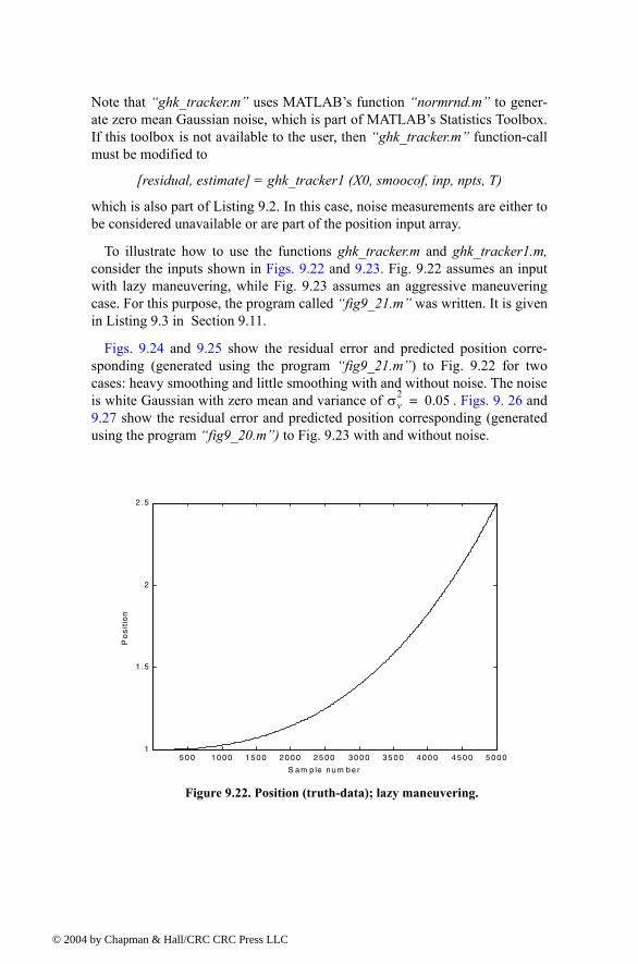
© 200
Note that ghk_tracker.m uses MATLABs function normrnd.m to gener-ate zero mean Gaussian noise, which is part of MATLABs Statistics Toolbox.If this toolbox is not available to the user, then ghk_tracker.m function-callmust be modified to
[residual, estimate] = ghk_tracker1 (X0, smoocof, inp, npts, T)
which is also part of Listing 9.2. In this case, noise measurements are either tobe considered unavailable or are part of the position input array.
To illustrate how to use the functions ghk_tracker.m and ghk_tracker1.m,consider the inputs shown in Figs. 9.22 and 9.23. Fig. 9.22 assumes an inputwith lazy maneuvering, while Fig. 9.23 assumes an aggressive maneuveringcase. For this purpose, the program called fig9_21.m was written. It is givenin Listing 9.3 in Section 9.11.
Figs. 9.24 and 9.25 show the residual error and predicted position corre-sponding (generated using the program fig9_21.m) to Fig. 9.22 for twocases: heavy smoothing and little smoothing with and without noise. The noiseis white Gaussian with zero mean and variance of . Figs. 9. 26 and9.27 show the residual error and predicted position corresponding (generatedusing the program fig9_20.m) to Fig. 9.23 with and without noise.
σv2 0.05=
Figure 9.22. Position (truth-data); lazy maneuvering.
5 0 0 1 0 0 0 1 50 0 2 0 0 0 2 5 0 0 3 0 0 0 3 5 0 0 4 0 0 0 4 5 0 0 5 0 0 01
1 .5
2
2 .5
Po
sit
ion
S a m p le n u m b e r
4 by Chapman & Hall/CRC CRC Press LLC
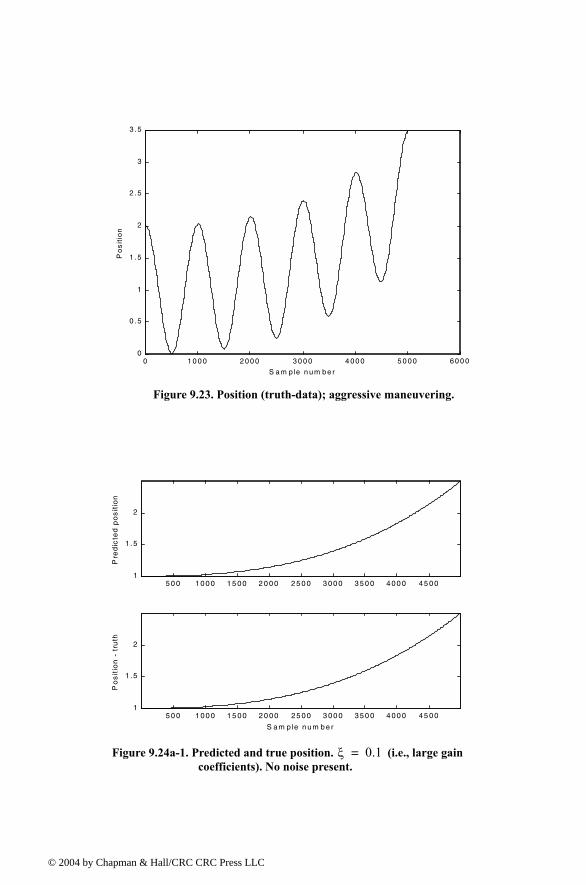
© 200
Figure 9.23. Position (truth-data); aggressive maneuvering.
0 1 0 0 0 2 0 0 0 3 0 0 0 4 0 0 0 5 0 0 0 6 0 0 00
0 .5
1
1 .5
2
2 .5
3
3 .5
S a m p le n u m b e r
Po
sit
ion
Figure 9.24a-1. Predicted and true position. (i.e., large gain coefficients). No noise present.
ξ 0.1=
50 0 1 00 0 1 5 00 2 0 00 25 0 0 3 00 0 3 50 0 4 00 0 45 001
1 .5
2
Pre
dic
ted
po
sit
ion
5 0 0 1 00 0 1 5 00 2 0 00 25 0 0 3 00 0 3 50 0 4 00 0 45 001
1 .5
2
S a m p le n u m b e r
Po
sit
ion
- t
ruth
4 by Chapman & Hall/CRC CRC Press LLC
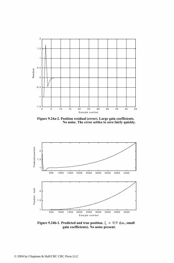
© 200
Figure 9.24a-2. Position residual (error). Large gain coefficients. No noise. The error settles to zero fairly quickly.
0 5 10 15 20 25 30 35 40 45 50-1 .5
-1
-0 .5
0
0 .5
1
1 .5
2
S am p le num ber
Re
sid
ua
l
Figure 9.24b-1. Predicted and true position. (i.e., small gain coefficients). No noise present.
ξ 0.9=
5 0 0 1 0 0 0 1 5 0 0 2 0 0 0 2 5 0 0 3 0 0 0 3 5 0 0 4 0 0 0 4 5 0 0
1
1 .5
2
Pre
dic
ted
po
sit
ion
5 0 0 1 0 0 0 1 5 0 0 2 0 0 0 2 5 0 0 3 0 0 0 3 5 0 0 4 0 0 0 4 5 0 01
1 .5
2
S a m p le n u m b e r
Po
sit
ion
- t
ruth
4 by Chapman & Hall/CRC CRC Press LLC
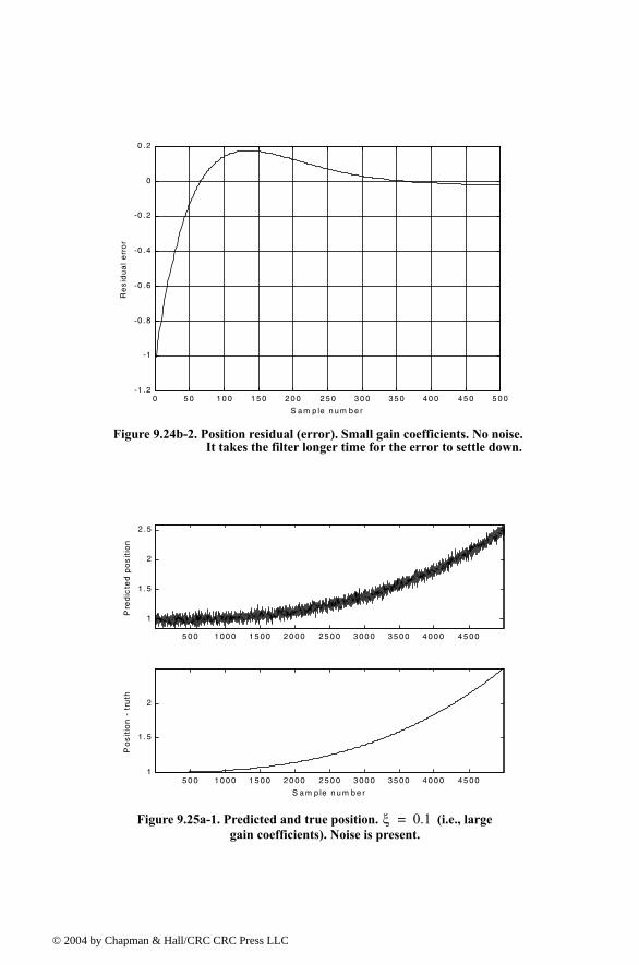
© 200
Figure 9.24b-2. Position residual (error). Small gain coefficients. No noise. It takes the filter longer time for the error to settle down.
0 5 0 1 0 0 1 5 0 2 0 0 2 5 0 3 0 0 3 5 0 4 0 0 4 5 0 5 0 0-1 .2
-1
-0 .8
-0 .6
-0 .4
-0 .2
0
0 .2
S a m p le n u m b e r
Re
sid
ua
l e
rro
r
Figure 9.25a-1. Predicted and true position. (i.e., large gain coefficients). Noise is present.
ξ 0.1=
50 0 1 00 0 1 5 00 2 0 00 25 0 0 3 00 0 3 50 0 4 00 0 45 00
1
1 .5
2
2 .5
Pre
dic
ted
po
sit
ion
5 0 0 1 00 0 1 5 00 2 0 00 25 0 0 3 00 0 3 50 0 4 00 0 45 001
1 .5
2
S a m p le n u m b e r
Po
sit
ion
- t
ruth
4 by Chapman & Hall/CRC CRC Press LLC
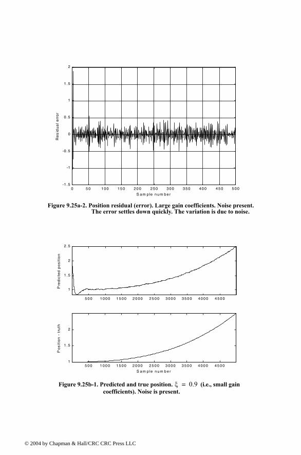
© 200
Figure 9.25a-2. Position residual (error). Large gain coefficients. Noise present. The error settles down quickly. The variation is due to noise.
0 50 1 00 15 0 20 0 250 3 00 3 50 40 0 45 0 5 00-1 .5
-1
-0 .5
0
0 .5
1
1 .5
2
S am p le nu m be r
Re
sid
ua
l e
rro
r
Figure 9.25b-1. Predicted and true position. (i.e., small gain coefficients). Noise is present.
ξ 0.9=
5 0 0 1 0 0 0 1 5 0 0 2 0 0 0 2 5 0 0 3 0 0 0 3 5 0 0 4 0 0 0 4 5 0 0
1
1 .5
2
2 .5
Pre
dic
ted
po
sit
ion
5 0 0 1 0 0 0 1 5 0 0 2 0 0 0 2 5 0 0 3 0 0 0 3 5 0 0 4 0 0 0 4 5 0 01
1 .5
2
S a m p le n u m b e r
Po
sit
ion
- t
ruth
4 by Chapman & Hall/CRC CRC Press LLC
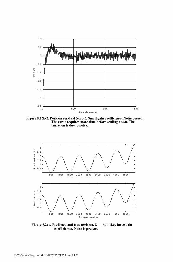
© 200
Figure 9.25b-2. Position residual (error). Small gain coefficients. Noise present. The error requires more time before settling down. The variation is due to noise.
0 500 1000 1500-1 .2
-1
-0 .8
-0 .6
-0 .4
-0 .2
0
0 .2
0 .4
S am p le num ber
Re
sid
ua
l
Figure 9.26a. Predicted and true position. (i.e., large gain coefficients). Noise is present.
ξ 0.1=
500 1000 1500 2000 2500 3000 3500 4000 4500
0 .5
1
1 .5
2
2 .5
3
Pre
dic
ted
po
sit
ion
5 00 1000 1500 2000 2500 3000 3500 4000 4500
0 .5
1
1 .5
2
2 .5
3
S am p le num ber
Po
sit
ion
- t
ruth
4 by Chapman & Hall/CRC CRC Press LLC
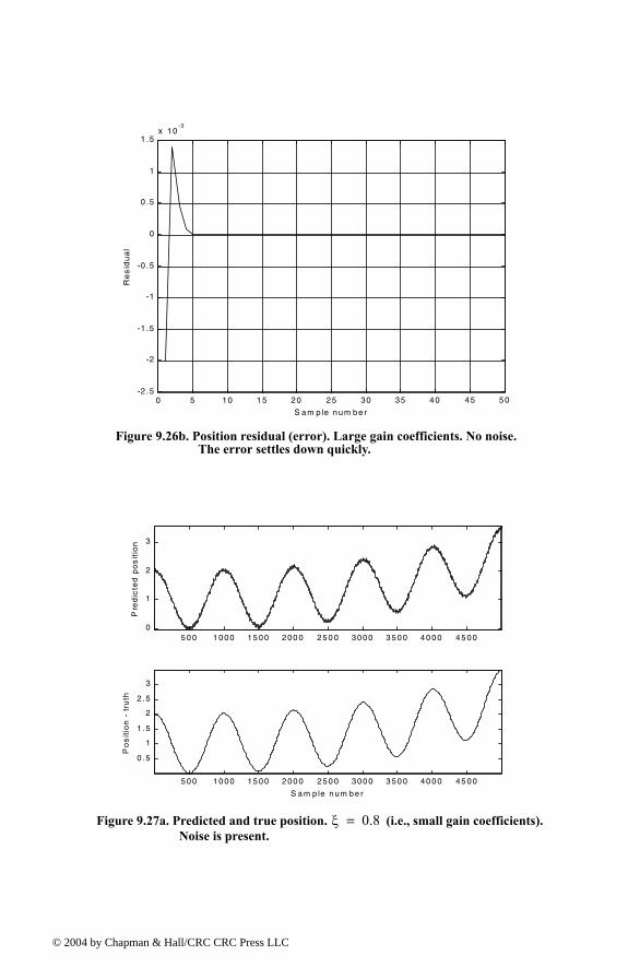
© 200
Figure 9.26b. Position residual (error). Large gain coefficients. No noise. The error settles down quickly.
0 5 10 1 5 20 25 30 35 4 0 4 5 50-2 .5
-2
-1 .5
-1
-0 .5
0
0 .5
1
1 .5x 10
-3R
es
idu
al
S a m p le num be r
Figure 9.27a. Predicted and true position. (i.e., small gain coefficients). Noise is present.
ξ 0.8=
5 0 0 1 0 0 0 1 5 0 0 2 0 0 0 2 5 0 0 3 0 0 0 3 5 0 0 4 0 0 0 4 5 0 00
1
2
3
Pre
dic
ted
po
sit
ion
5 0 0 1 0 0 0 1 5 0 0 2 0 0 0 2 5 0 0 3 0 0 0 3 5 0 0 4 0 0 0 4 5 0 0
0 .5
1
1 .5
2
2 .5
3
S a m p le n u m b e r
Po
sit
ion
- t
ruth
4 by Chapman & Hall/CRC CRC Press LLC
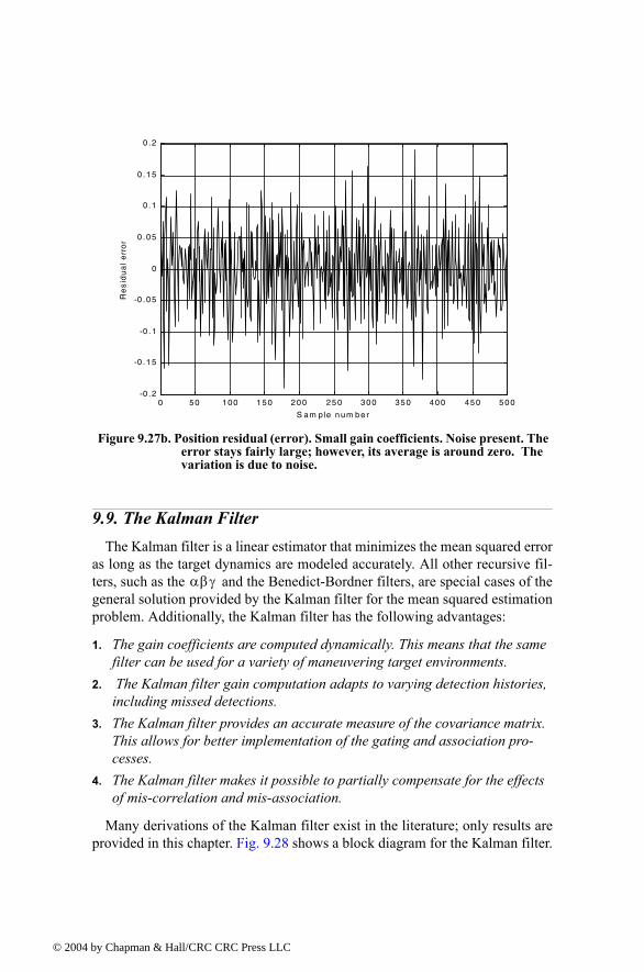
© 200
9.9. The Kalman FilterThe Kalman filter is a linear estimator that minimizes the mean squared error
as long as the target dynamics are modeled accurately. All other recursive fil-ters, such as the and the Benedict-Bordner filters, are special cases of thegeneral solution provided by the Kalman filter for the mean squared estimationproblem. Additionally, the Kalman filter has the following advantages:
1. The gain coefficients are computed dynamically. This means that the same filter can be used for a variety of maneuvering target environments.
2. The Kalman filter gain computation adapts to varying detection histories, including missed detections.
3. The Kalman filter provides an accurate measure of the covariance matrix. This allows for better implementation of the gating and association pro-cesses.
4. The Kalman filter makes it possible to partially compensate for the effects of mis-correlation and mis-association.
Many derivations of the Kalman filter exist in the literature; only results areprovided in this chapter. Fig. 9.28 shows a block diagram for the Kalman filter.
Figure 9.27b. Position residual (error). Small gain coefficients. Noise present. The error stays fairly large; however, its average is around zero. The variation is due to noise.
0 50 100 150 200 250 300 350 400 450 500-0 .2
-0 .15
-0 .1
-0 .05
0
0 .05
0 .1
0 .15
0 .2
S am p le num ber
Re
sid
ua
l e
rro
r
αβγ
4 by Chapman & Hall/CRC CRC Press LLC
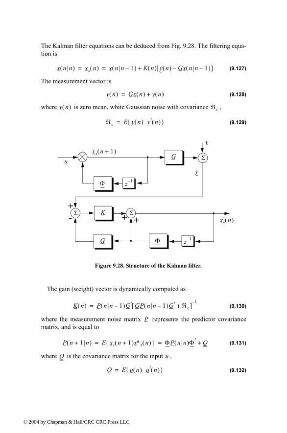
© 200
The Kalman filter equations can be deduced from Fig. 9.28. The filtering equa-tion is
(9.127)
The measurement vector is
(9.128)
where is zero mean, white Gaussian noise with covariance ,
(9.129)
The gain (weight) vector is dynamically computed as
(9.130)
where the measurement noise matrix represents the predictor covariancematrix, and is equal to
(9.131)
where is the covariance matrix for the input ,
(9.132)
x n n( ) xs n( ) x n n 1( ) K n( ) y n( ) Gx n n 1( )[ ]+= =
y n( ) Gx n( ) v n( )+=
v n( ) ℜc
ℜc E y n( ) yt n( ) =
Σu
Φ
G
y
xs n 1+( )v
z 1
z 1
Σ ΣK
G Φ
+- + + xs n( )
Figure 9.28. Structure of the Kalman filter.
K n( ) P n n 1( )Gt GP n n 1( )Gt ℜc+[ ]1
=
P
P n 1+ n( ) E xs n 1+( )x∗s n( ) ΦP n n( )Φt
Q+= =
Q u
Q E u n( ) ut n( ) =
4 by Chapman & Hall/CRC CRC Press LLC
© 200
The corrector equation (covariance of the smoothed estimate) is
(9.133)
Finally, the predictor equation is
(9.134)
9.9.1. The Singer -Kalman Filter
The Singer1 filter is a special case of the Kalman where the filter is gov-erned by a specified target dynamic model whose acceleration is a random pro-cess with autocorrelation function given by
(9.135)
where is the correlation time of the acceleration due to target maneuveringor atmospheric turbulence. The correlation time may vary from as low as10 seconds for aggressive maneuvering to as large as 60 seconds for lazymaneuvering cases.
Singer defined the random target acceleration model by a first order Markovprocess given by
(9.136)
where is a zero mean, Gaussian random variable with unity variance, is the maneuver standard deviation, and the maneuvering correlation coef-
ficient is given by
(9.137)
The continuous time domain system that corresponds to these conditions is thesame as the Wiener-Kolmogorov whitening filter which is defined by the dif-ferential equation
(9.138)
1. Singer, R. A., Estimating Optimal Tracking Filter Performance for Manned Maneu-vering Targets, IEEE Transaction on Aerospace and Electronics, AES-5, July, 1970, pp. 473-483.
P n n( ) I K n( )G[ ]P n n 1( )=
x n 1+ n( ) Φx n n( )=
αβγ
E x·· t( ) x·· t t1+( ) σa2 e
t1τm------
=
τmτm
x·· n 1+( ) ρm x·· n( ) 1 ρm2 σm w n( )+=
w n( )σm
ρm
ρm eTτm-----
=
tdd v t( ) βmv t( ) w t( )+=
4 by Chapman & Hall/CRC CRC Press LLC
© 200
where is equal to . The maneuvering variance using Singers modelis given by
(9.139)
is the maximum target acceleration with probability and the term defines the probability that the target has no acceleration.
The transition matrix that corresponds to the Singer filter is given by
(9.140)
Note that when is small (the target has constant acceleration),then Eq. (9.140) reduces to Eq. (9.114). Typically, the sampling interval ismuch less than the maneuvering time constant ; hence, Eq. (9.140) can beaccurately replaced by its second order approximation. More precisely,
(9.141)
The covariance matrix was derived by Singer, and it is equal to
(9.142)
where
(9.143)
(9.144)
(9.145)
βm 1 τm⁄
σm2 Amax
2
3----------- 1 4Pmax P0+[ ]=
Amax PmaxP0
Φ
1 T 1βm
2------ 1 βmT ρm+ +( )
0 1 1βm------ 1 ρm( )
0 0 ρm
=
Tβm T τm⁄=T
τm
Φ1 T T2 2⁄0 1 T 1 T 2τm⁄( )
0 0 ρm
=
C2σm
2
τm----------
C11 C12 C13
C21 C22 C23
C31 C32 C33
=
C11 σx2 1
2βm5
--------- 1 e2βmT
2βmT2βm
3 T3
3--------------- 2βm
2 T2 4βmTeβmT
+ += =
C12 C211
2βm4
--------- e2βmT
1+ 2 eβmT
2βmTeβmT
2βmT βm2 T2++[ ]= =
C13 C311
2βm3
--------- 1 e2βmT
2 βmTeβmT
[ ]= =
4 by Chapman & Hall/CRC CRC Press LLC
© 200
(9.146)
(9.147)
(9.148)
Two limiting cases are of interest:
1. The short sampling interval case ( ),
(9.149)
and the state transition matrix is computed from Eq. (9.141) as
(9.150)
which is the same as the case for the filter (constant acceleration).
2. The long sampling interval ( ). This condition represents the case when acceleration is a white noise process. The corresponding covariance and transition matrices are, respectively, given by
(9.151)
(9.152)
Note that under the condition that , the cross correlation terms and become very small. It follows that estimates of acceleration are no longer
C221
2βm3
--------- 4eβmT
3 e2βmT
2βmT+[ ]=
C23 C321
2βm2
--------- e2βmT
1 2eβmT
+[ ]= =
C331
2βm--------- 1 e
2βmT[ ]=
T τm«
CβmT 0→
lim2σm
2
τm----------
T5 20⁄ T4 8⁄ T3 6⁄
T4 8⁄ T3 3⁄ T2 2⁄
T3 6⁄ T2 2⁄ T
=
ΦβmT 0→
lim1 T T2 2⁄0 1 T0 0 1
=
αβγ
T τm»
CβmT ∞→
lim σm2
2T3τm
3--------------- T2τm τm
2
T2τm 2Tτm τm
τm2 τm 1
=
ΦβmT ∞→
lim1 T Tτm
0 1 τm
0 0 0
=
T τm» C13C23
4 by Chapman & Hall/CRC CRC Press LLC
© 200
available, and thus a two state filter model can be used to replace the three statemodel. In this case,
(9.153)
(9.154)
9.9.2. Relationship between Kalman and Filters
The relationship between the Kalman filter and the filters can be easilyobtained by using the appropriate state transition matrix , and gain vector corresponding to the in Eq. (9.127). Thus,
(9.155)
with (see Fig. 9.21)
(9.156)
(9.157)
(9.158)
Comparing the previous three equations with the filter equations yields
(9.159)
Additionally, the covariance matrix elements are related to the gain coeffi-cients by
C 2σm2 τm
T3 3⁄ T2 2⁄
T2 2⁄ T=
Φ 1 T0 1
=
αβγαβγΦ K
αβγ
x n n( )x· n n( )x·· n n( )
x n n 1( )x· n n 1( )x·· n n 1( )
k1 n( )
k2 n( )
k3 n( )
x0 n( ) x n n 1( )[ ]+=
x n n 1( ) xs n 1( ) T x· s n 1( ) T2
2----- x··s n 1( )+ +=
x· n n 1( ) x· s n 1( ) T x··s n 1( )+=
x·· n n 1( ) x··s n 1( )=
αβγ
αβT---
γ
T2-----
k1
k2
k3
=
4 by Chapman & Hall/CRC CRC Press LLC
© 200
(9.160)
Eq. (9.160) indicates that the first gain coefficient depends on the estimationerror variance of the total residual variance, while the other two gain coeffi-cients are calculated through the covariances between the second and thirdstates and the first observed state.
MATLAB Function kalman_filter.m
The function kalman_filter.m implements a state Singer- Kalman fil-ter. It is given in Listing 9.4 in Section 9.11. The syntax is as follows:
[residual, estimate] = kalman_filter(npts, T, X0, inp, R, nvar)
where
Note that kalman_filter.m uses MATLABs function normrnd.m to gener-ate zero mean Gaussian noise, which is part of MATLABs Statistics Toolbox.
To illustrate how to use the functions kalman_filter.m, consider the inputsshown in Figs. 9.22 and 9.23. Figs. 9.29 and 9.30 show the residual error andpredicted position corresponding to Figs. 9.22 and 9.23. These plots can bereproduced using the program fig9_28.m given in Listing 9.5 in Section9.11.
Symbol Description Status
npts number of points in input position input
T sampling interval input
X0 initial state vector input
inp input array input
R noise variance see Eq. (9-129) input
nvar desired state noise variance input
residual array of position error (residual) output
estimate array of predicted position output
k1
k2
k3
1C11 σv
2+--------------------
C11
C12
C13
=
αβγ
4 by Chapman & Hall/CRC CRC Press LLC
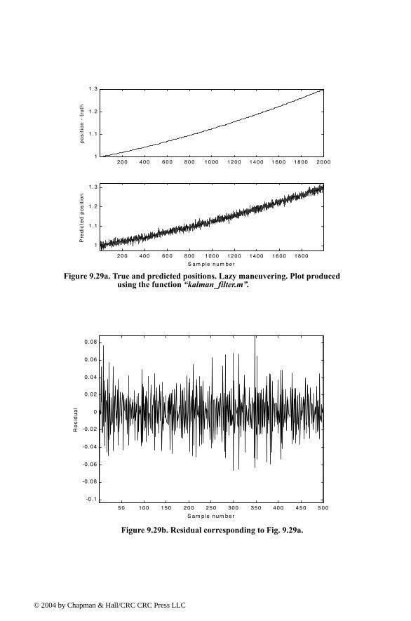
© 200
20 0 4 00 6 0 0 8 0 0 10 00 1 20 0 1 40 0 1 60 0 1 8 00 20 0 01
1 .1
1 .2
1 .3
po
sit
ion
- t
ruth
2 0 0 4 00 6 0 0 8 0 0 10 0 0 1 20 0 1 40 0 1 6 00 18 00
1
1 .1
1 .2
1 .3
S a m p le n u m b e r
Pre
dic
ted
po
sit
ion
Figure 9.29a. True and predicted positions. Lazy maneuvering. Plot produced using the function kalman_filter.m.
50 100 150 200 250 300 350 400 450 500
-0.1
-0 .08
-0 .06
-0 .04
-0 .02
0
0.02
0.04
0.06
0.08
S am ple num ber
Re
sid
ua
l
Figure 9.29b. Residual corresponding to Fig. 9.29a.
4 by Chapman & Hall/CRC CRC Press LLC
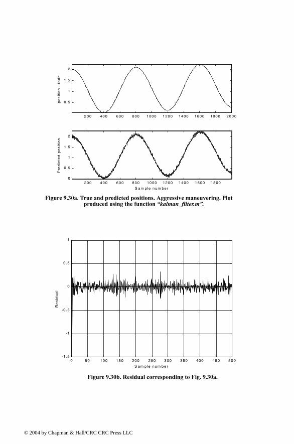
© 200
2 00 40 0 60 0 80 0 100 0 120 0 1 40 0 16 00 18 00 200 0
0 .5
1
1 .5
2
po
sit
ion
- t
ruth
2 00 40 0 60 0 80 0 10 00 120 0 1 40 0 1 600 18 000
0 .5
1
1 .5
2
S am p le nu m be r
Pre
dic
ted
po
sit
ion
Figure 9.30a. True and predicted positions. Aggressive maneuvering. Plot produced using the function kalman_filter.m.
0 50 100 150 200 250 300 350 400 450 500-1 .5
-1
-0 .5
0
0 .5
1
S am p le num ber
Re
sid
ua
l
Figure 9.30b. Residual corresponding to Fig. 9.30a.
4 by Chapman & Hall/CRC CRC Press LLC

© 200
9.10. MyRadar Design Case Study - Visit 9
9.10.1.Problem Statement
Implement a Kalman filter tracker into the MyRadar design case study.
9.10.2. A Design1
For this purpose, the MATLAB GUI workspace entitled kalman_gui.mwas developed. It is shown in Fig. 9.31. In this design, the inputs can be initial-ized to correspond to either target type (aircraft and missile). For example,when you click on the button ResetMissile, the initial x-, y-, and z-detectioncoordinates for the missile are loaded into the Starting Location field. Thecorresponding target velocity is also loaded in the velocity in x directionfield. Finally, all other fields associated with the Kalman filter are also loadedusing default values that are appropriate for this design case study. Note thatthe user can alter these entries as appropriate.
This program generates a fictitious trajectory for the selected target type.This is accomplished using the function maketraj.m. It is given in Listing9.6 in Section 9.11. The user can either use this program, or import their ownspecific trajectory. The function maketraj.m assumes constant altitude, andgenerates a manuevering trajectory in the x-y plane, as shown in Fig. 9.32. Thistrajectory can be changed using the different fields in the trajectory Parame-ter fields.
Next the program corrupts the trajectory by adding white Guassian noise toit. This is accomplished by the function addnoise.m which is given in List-ing 9.7 in Section 9.11. A six-state Kalman filter named kalfilt.m is then uti-lized to perform the tracking task. This function is given in Listing 9.8.
The azimuth, elevation, and range errors are input to the program using theircorresponding fields on the GUI. In this example, these entries are assumedconstant throughout the simulation. In practice, this is not true and these valueswill change. They are caluclated by the radar signal processor on a per pro-cessing interval basis and then are input into the tracker. For example, thestandard deviation of the error in the range measurement is
(9.161)
1. The MATLAB code in this section was developed by Mr. David Hall, Consultant to Decibel Research, Inc., Huntsville, Alabama.
σR∆R
2 SNR×------------------------ c
2B 2 SNR×--------------------------------= =
4 by Chapman & Hall/CRC CRC Press LLC
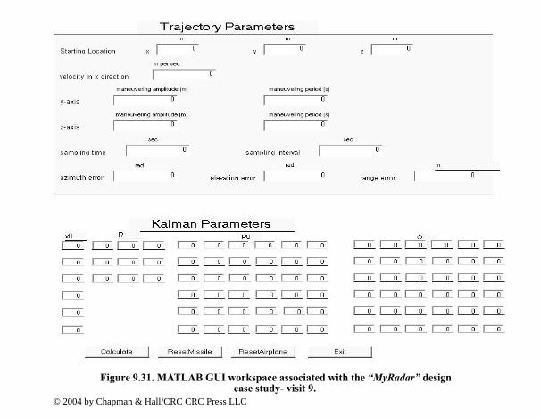
adar design
© 2004 by Chapman & Hall/CRC CRC Press LLC
Figure 9.31. MATLAB GUI workspace associated with the MyRcase study- visit 9.
© 200
where is the range resolution, is the speed of light, is the bandwidth,and is the measurement SNR.
The standard deviation of the error in the velocity measurement is
(9.162)
where is the wavelength and is the uncompressed pulsewidth. The stan-dard deviation of the error in the angle measurement is
(9.163)
where is the antenna beamwidth of the angular coordinate of the measure-ment (azimuth and elevation).
In this example, the radar is located at . This simulationcalculates and plots the following outputs:
Fig. 9.32 through Fig. 9.42 shows typical outputs produced using this simu-lation for the missile.
TABLE 9.1. Output list generated by the kalman_gui.m simulation
Figure # Description
9.32 uncorrupted input trajectory
9.33 corrupted input trajectory
9.34 corrupted and uncorrupted x-position
9.35 corrupted and uncorrupted y-position
9.36 corrupted and uncorrupted z-position
9.37 corrupted and filtered x-, y- and z-positions
9.38 predicted x-, y-, and z- velocities
9.39 position residuals
9.40 velocity residuals
9.41 covariance matrix components versus time
9.42 Kalman filter gains versus time
∆R c BSNR
σvλ
2τ 2 SNR×-------------------------------=
λ τ
σaΘ
1.6 2 SNR×--------------------------------=
Θ
x y z, ,( ) 0 0 0, ,( )=
4 by Chapman & Hall/CRC CRC Press LLC
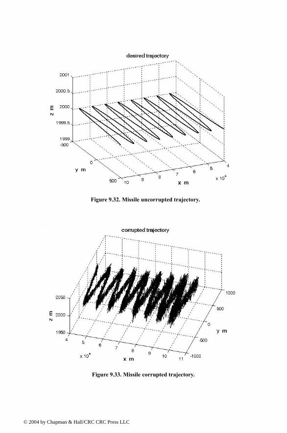
© 200
Figure 9.32. Missile uncorrupted trajectory.
Figure 9.33. Missile corrupted trajectory.
4 by Chapman & Hall/CRC CRC Press LLC
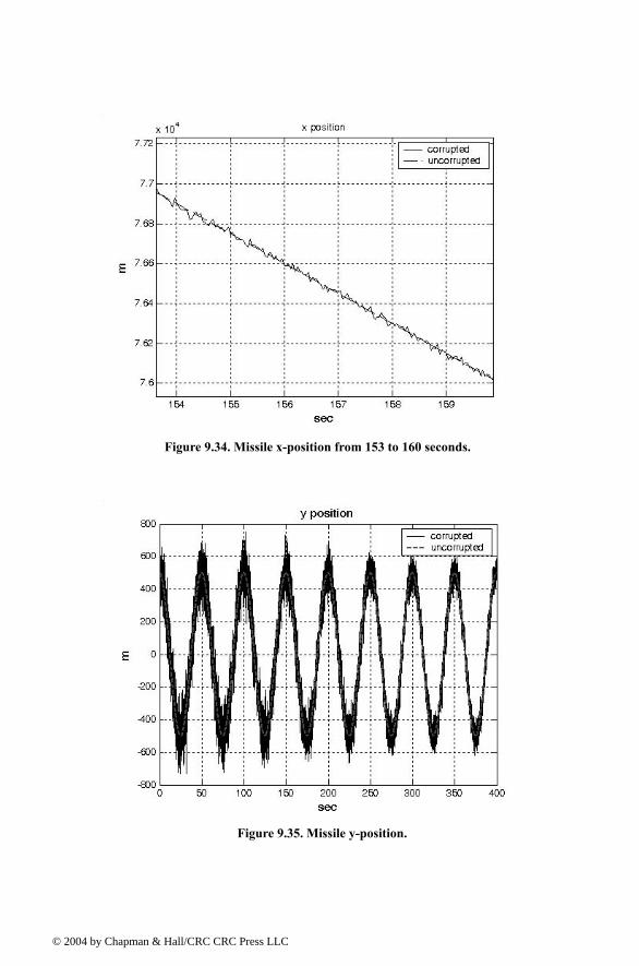
© 200
Figure 9.34. Missile x-position from 153 to 160 seconds.
Figure 9.35. Missile y-position.
4 by Chapman & Hall/CRC CRC Press LLC
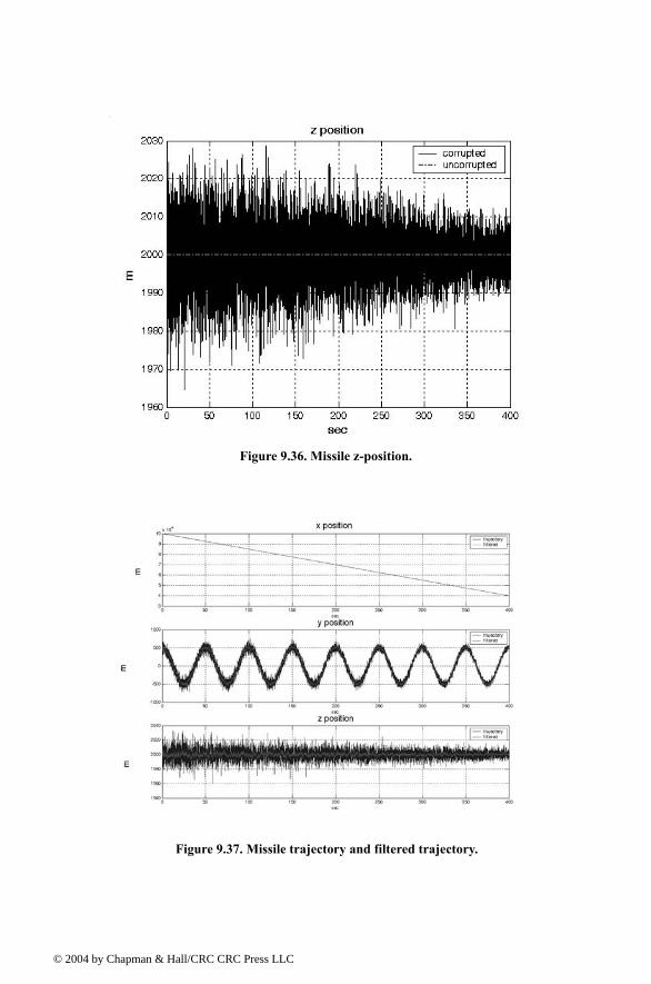
© 200
Figure 9.36. Missile z-position.
Figure 9.37. Missile trajectory and filtered trajectory.
4 by Chapman & Hall/CRC CRC Press LLC
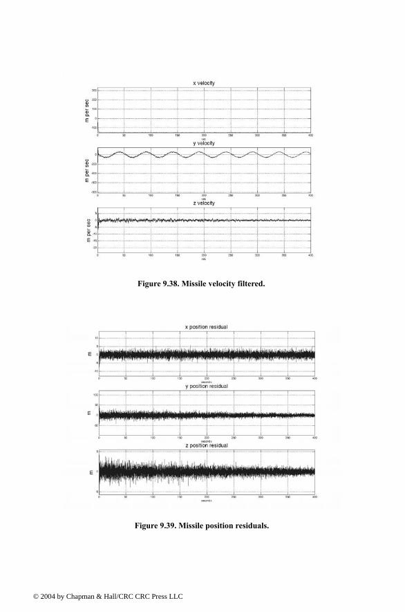
© 200
Figure 9.38. Missile velocity filtered.
Figure 9.39. Missile position residuals.
4 by Chapman & Hall/CRC CRC Press LLC
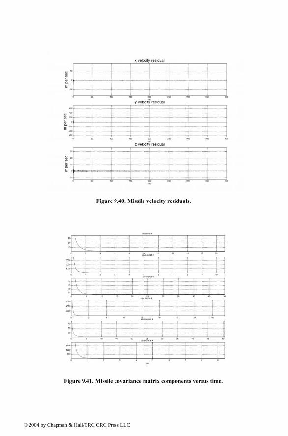
© 200
Figure 9.40. Missile velocity residuals.
Figure 9.41. Missile covariance matrix components versus time.
4 by Chapman & Hall/CRC CRC Press LLC
© 200
9.11. MATLAB Program and Function ListingsThis section contains listings of all MATLAB programs and functions used
in this chapter. Users are encouraged to rerun this code with different inputs inorder to enhance their understanding of the theory.
Listing 9.1. MATLAB Function mono_pulse.mfunction mono_pulse(phi0)eps = 0.0000001;angle = -pi:0.01:pi;y1 = sinc(angle + phi0);y2 = sinc((angle - phi0));ysum = y1 + y2;ydif = -y1 + y2;figure (1)plot (angle,y1,'k',angle,y2,'k');grid;xlabel ('Angle - radians')ylabel ('Squinted patterns')
Figure 9.42. Kalman filter gains versus time.
4 by Chapman & Hall/CRC CRC Press LLC
© 200
figure (2)plot(angle,ysum,'k');grid;xlabel ('Angle - radians')ylabel ('Sum pattern')figure (3)plot (angle,ydif,'k');grid;xlabel ('Angle - radians')ylabel ('Difference pattern')angle = -pi/4:0.01:pi/4;y1 = sinc(angle + phi0);y2 = sinc((angle - phi0));ydif = -y1 + y2;ysum = y1 + y2;dovrs = ydif ./ ysum;figure(4)plot (angle,dovrs,'k');grid;xlabel ('Angle - radians')ylabel ('voltage gain')
Listing 9.2. MATLAB Function ghk_tracker.mfunction [residual, estimate] = ghk_tracker (X0, smoocof, inp, npts, T, nvar)rn = 1.;% read the initial estimate for the state vectorX = X0; theta = smoocof;%compute values for alpha, beta, gammaw1 = 1. - (theta^3);w2 = 1.5 * (1. + theta) * ((1. - theta)^2) / T;w3 = ((1. - theta)^3) / (T^2);% setup the transition matrix PHIPHI = [1. T (T^2)/2.;0. 1. T;0. 0. 1.];while rn < npts ; %use the transition matrix to predict the next state XN = PHI * X; error = (inp(rn) + normrnd(0,nvar)) - XN(1); residual(rn) = error; tmp1 = w1 * error; tmp2 = w2 * error; tmp3 = w3 * error; % compute the next state
4 by Chapman & Hall/CRC CRC Press LLC
© 200
X(1) = XN(1) + tmp1; X(2) = XN(2) + tmp2; X(3) = XN(3) + tmp3; estimate(rn) = X(1); rn = rn + 1.;endreturn
MATLAB Function ghk_tracker1.m
function [residual, estimate] = ghk_tracker1 (X0, smoocof, inp, npts, T)rn = 1.;% read the initial estimate for the state vectorX = X0; theta = smoocof;%compute values for alpha, beta, gammaw1 = 1. - (theta^3);w2 = 1.5 * (1. + theta) * ((1. - theta)^2) / T;w3 = ((1. - theta)^3) / (T^2);% setup the transition matrix PHIPHI = [1. T (T^2)/2.;0. 1. T;0. 0. 1.];while rn < npts ; %use the transition matrix to predict the next state XN = PHI * X; error = inp(rn) - XN(1); residual(rn) = error; tmp1 = w1 * error; tmp2 = w2 * error; tmp3 = w3 * error; % compute the next state X(1) = XN(1) + tmp1; X(2) = XN(2) + tmp2; X(3) = XN(3) + tmp3; estimate(rn) = X(1); rn = rn + 1.;endreturn
Listing 9.3. MATLAB Program fig9_21.mclear alleps = 0.0000001;npts = 5000;del = 1./ 5000.;t = 0. : del : 1.;
4 by Chapman & Hall/CRC CRC Press LLC
© 200
% generate input sequenceinp = 1.+ t.^3 + .5 .*t.^2 + cos(2.*pi*10 .* t) ;% read the initial estimate for the state vectorX0 = [2,.1,.01]';% this is the update interval in secondsT = 100. * del;% this is the value of the smoothing coefficientxi = .91;[residual, estimate] = ghk_tracker (X0, xi, inp, npts, T, .01);figure(1)plot (residual(1:500))xlabel ('Sample number')ylabel ('Residual error')gridfigure(2)NN = 4999.;n = 1:NN;plot (n,estimate(1:NN),'b',n,inp(1:NN),'r')xlabel ('Sample number')ylabel ('Position')legend ('Estimated','Input')
Listing 9.4. MATLAB Function kalman_filter.mfunction [residual, estimate] = kalman_filter(npts, T, X0, inp, R, nvar)N = npts;rn=1;% read the initial estimate for the state vectorX = X0;% it is assumed that the measurement vector H=[1,0,0]% this is the state noise varianceVAR = nvar;% setup the initial value for the prediction covariance.S = [1. 1. 1.; 1. 1. 1.; 1. 1. 1.];% setup the transition matrix PHIPHI = [1. T (T^2)/2.; 0. 1. T; 0. 0. 1.];% setup the state noise covariance matrixQ(1,1) = (VAR * (T^5)) / 20.;Q(1,2) = (VAR * (T^4)) / 8.;Q(1,3) = (VAR * (T^3)) / 6.;Q(2,1) = Q(1,2);Q(2,2) = (VAR * (T^3)) / 3.;Q(2,3) = (VAR * (T^2)) / 2.;Q(3,1) = Q(1,3);
4 by Chapman & Hall/CRC CRC Press LLC
© 200
Q(3,2) = Q(2,3);Q(3,3) = VAR * T;while rn < N ; %use the transition matrix to predict the next state XN = PHI * X; % Perform error covariance extrapolation S = PHI * S * PHI' + Q; % compute the Kalman gains ak(1) = S(1,1) / (S(1,1) + R); ak(2) = S(1,2) / (S(1,1) + R); ak(3) = S(1,3) / (S(1,1) + R); %perform state estimate update: error = inp(rn) + normrnd(0,R) - XN(1); residual(rn) = error; tmp1 = ak(1) * error; tmp2 = ak(2) * error; tmp3 = ak(3) * error; X(1) = XN(1) + tmp1; X(2) = XN(2) + tmp2; X(3) = XN(3) + tmp3; estimate(rn) = X(1); % update the error covariance S(1,1) = S(1,1) * (1. -ak(1)); S(1,2) = S(1,2) * (1. -ak(1)); S(1,3) = S(1,3) * (1. -ak(1)); S(2,1) = S(1,2); S(2,2) = -ak(2) * S(1,2) + S(2,2); S(2,3) = -ak(2) * S(1,3) + S(2,3); S(3,1) = S(1,3); S(3,3) = -ak(3) * S(1,3) + S(3,3); rn = rn + 1.;end
Listing 9.5. MATLAB Program fig9_28.mclear allnpts = 2000;del = 1/2000;t = 0:del:1;inp = (1+.2 .* t + .1 .*t.^2) + cos(2. * pi * 2.5 .* t);X0 = [1,.1,.01]';% it is assumed that the measurement vector H=[1,0,0]% this is the update interval in secondsT = 1.;
4 by Chapman & Hall/CRC CRC Press LLC
© 200
% enter the measurement noise varianceR = .035;% this is the state noise variancenvar = .5;[residual, estimate] = kalman_filter(npts, T, X0, inp, R, nvar);figure(1)plot(residual)xlabel ('Sample number')ylabel ('Residual')figure(2)subplot(2,1,1)plot(inp)axis tightylabel ('position - truth')subplot(2,1,2)plot(estimate)axis tightxlabel ('Sample number')ylabel ('Predicted position')
Listing 9.6. MATLAB Function maketraj.mfunction [times , trajectory] = maketraj(start_loc, xvelocity, yamp, yperiod, zamp, zperiod, samplingtime, deltat)% maketraj.m% by David J. Hall% for Bassem Mahafza% 17 June 2003% 17:01% USAGE: [times , trajectory] = maketraj(start_loc, xvelocity, yamp, yperiod, zamp, zperiod, samplingtime, deltat)% NOTE: all coordinates are in radar reference coordinates.% INPUTS% name dimension explanation units%------ ------ --------------- -------% start_loc 3 X 1 starting location of target m% xvelocity 1 velocity of target m/s% yamp 1 amplitude of oscillation y direction m% yperiod 1 period of oscillation y direction m% zamp 1 amplitude of oscillation z direction m% zperiod 1 period of oscillation z direction m% samplingtime 1 length of interval of trajectory sec% deltat 1 time between samples sec%
4 by Chapman & Hall/CRC CRC Press LLC
© 200
% OUTPUTS%% name dimension explanation units%------ ---------- --------------- ------% times 1 X samplingtime/deltat vector of times % corresponding to samples sec% trajectory 3 X samplingtime/deltat trajectory x,y,z m%times = 0: deltat: samplingtime ;x = start_loc(1)+xvelocity.*times ;if yperiod~=0 y = start_loc(2)+yamp*cos(2*pi*(1/yperiod).*times) ;else y = ones(1, length(times))*start_loc(2) ;endif zperiod~=0 z = start_loc(3)+zamp*cos(2*pi*(1/zperiod).*times) ;else z = ones(1, length(times))*start_loc(3) ; endtrajectory = [x ; y ; z] ;
Listing 9.7. MATLAB Function addnoise.mfunction [noisytraj ] = addnoise(trajectory, sigmaaz, sigmael, sigmarange )% addnoise.m% by David J. Hall% for Bassem Mahafza% 10 June 2003% 11:46% USAGE: [noisytraj ] = addnoise(trajectory, sigmaaz, sigmael, sigmarange )% INPUTS% name dimension explanation units%------ ------ --------------- -------% trajectory 3 X POINTS trajectory in radar reference coords [m;m;m]% sigmaaz 1 standard deviation of azimuth error radians% sigmael 1 standard deviation of elevation error radians% sigmarange 1 standard deviation of range error m%% OUTPUTS% name dimension explanation units%------ ------ --------------- -------% noisytraj 3 X POINTS noisy trajectory [m;m;m]noisytraj = zeros(3, size(trajectory,2)) ;
4 by Chapman & Hall/CRC CRC Press LLC

© 200
for loop = 1 : size(trajectory,2) x = trajectory(1,loop); y = trajectory(2,loop); z = trajectory(3,loop); azimuth_corrupted = atan2(y,x) + sigmaaz*randn(1) ; elevation_corrupted = atan2(z, sqrt(x^2+y^2)) + sigmael*randn(1) ; range_corrupted = sqrt(x^2+y^2+z^2) + sigmarange*randn(1) ; x_corrupted = range_corrupted*cos(elevation_corrupted)*cos(azimuth_corrupted) ; y_corrupted = range_corrupted*cos(elevation_corrupted)*sin(azimuth_corrupted) ; z_corrupted = range_corrupted*sin(elevation_corrupted) ; noisytraj(:,loop) = [x_corrupted ; y_corrupted; z_corrupted ] ;end % next loop
Listing 9.8. MATLAB Function kalfilt.mfunction [filtered, residuals , covariances, kalmgains] = kalfilt(trajectory, x0, P0, phi, R, Q )% kalfilt.m% by David J. Hall% for Bassem Mahafza% 10 June 2003% 11:46% USAGE: [filtered, residuals , covariances, kalmgains] = kalfilt(trajectory, x0, P0, phi, R, Q )%% INPUTS% name dimension explanation units%------ ------ --------------- -------% trajectory NUMMEASUREMENTS X NUMPOINTS trajectory in radar reference coords [m;m;m]% x0 NUMSTATES X 1 initial estimate of state vector m, m/s% P0 NUMSTATES X NUMSTATES initial estimate of covariance matrix m, m/s% phi NUMSTATES X NUMSTATES state transition matrix -% R NUMMEASUREMENTS X NUMMEASUREMENTS measurement error covariance matrix m% Q NUMSTATES X NUMSTATES state error covariance matrix m, m/s%
4 by Chapman & Hall/CRC CRC Press LLC

© 200
% OUTPUTS% name dimension explanation units%------ ------ --------------- -------% filtered NUMSTATES X NUMPOINTS filtered trajectory x,y,z pos, vel [m; m/s; m; m/s; m; m/s]% residuals NUMSTATES X NUMPOINTS residuals of filtering [m;m;m]% covariances NUMSTATES X NUMPOINTS diagonal of covariance matrix [m;m;m]% kalmgains (NUMSTATES X NUMMEASUREMENTS) % X NUMPOINTS Kalman gain matrix -NUMSTATES = 6 ;NUMMEASUREMENTS = 3 ;NUMPOINTS = size(trajectory, 2) ;% initialize output matricesfiltered = zeros(NUMSTATES, NUMPOINTS) ;residuals = zeros(NUMSTATES, NUMPOINTS) ;covariances = zeros(NUMSTATES, NUMPOINTS) ;kalmgains = zeros(NUMSTATES*NUMMEASUREMENTS, NUMPOINTS) ;% set matrix relating measurements to statesH = [1 0 0 0 0 0 ; 0 0 1 0 0 0 ; 0 0 0 0 1 0];xhatminus = x0 ;Pminus = P0 ; for loop = 1: NUMPOINTS % compute the Kalman gain K = Pminus*H'*inv(H*Pminus*H' + R) ; kalmgains(:,loop) = reshape(K, NUMSTATES*NUMMEASUREMENTS, 1) ; % update the estimate with the measurement z z = trajectory(:,loop) ; xhat = xhatminus + K*(z - H*xhatminus) ; filtered(:,loop) = xhat ; residuals(:,loop) = xhat - xhatminus ; % update the error covariance for the updated estimate P = ( eye(NUMSTATES, NUMSTATES) - K*H)*Pminus ; covariances(:,loop) = diag(P) ; % only save diagonal of covariance matrix % project ahead xhatminus_next = phi*xhat ; Pminus_next = phi*P*phi' + Q ; xhatminus = xhatminus_next ; Pminus = Pminus_next ;end
4 by Chapman & Hall/CRC CRC Press LLC
© 200
Chapter 10 Electronic Countermeasures (ECM)
This chapter is coauthored with J. Michael Madewell1
10.1. IntroductionAny deliberate electronic effort intended to disturb normal radar operation is
usually referred to as an Electronic Countermeasure (ECM). This may also include chaff, radar decoys, radar RCS alterations (e.g., radio frequency absorbing materials), and, of course, radar jamming.
In general, ECM is used by the offense to accomplish one, several, or possi-bly all of the following objectives: (1) deny proper target detection; (2) gener-ate operator confusion and / or deception; (3) force delays in detection and tracking initiation; (4) generate false tracks of non-real targets; (5) overload the radar computer with an excessive number of targets; (6) deny accurate measurements of the target range and range rate; (7) force dropped tracks; and (8) introduce errors in target position and range rate. Alternatively, the defense may utilize Electronic counter-countermeasures (ECCM) to overcome and mitigate the effects of ECM on the radar. When deployed properly, ECCM techniques and / or hardware can have the following effects: (1) prevent receiver saturation; (2) maintain a reasonable CFAR rate; (3) enhance the sig-nal to jammer ratio; (4) properly identify and discriminate directional interfer-ence; (5) reject invalid targets; and (6) maintain true target tracks.
ECM techniques can be exploited by a radar system in many different ways and can be categorized into two classes:
1. Mr. J. Michael Madewell is with the US Army Space and Missile Defense Com-mand in Huntsville, Alabama.
4 by Chapman & Hall/CRC CRC Press LLC
© 200
1. Denial ECM techniques: Denial ECM techniques can be either active or passive. Active denial ECM techniques include: CW, short pulse, long pulse, spot noise, barrage noise, and sidelobe repeaters. Passive ECM tech-niques include chaff and Radar Absorbing Material (RAM).
2. Deception ECM techniques: Deception ECM techniques are also broken down into active and passive techniques. Active deception ECM techniques include repeater jammers and false target generators. Passive deception ECM include chaff and RAM.
10.2. JammersJammers can be categorized into two general types: (1) barrage jammers and
(2) deceptive jammers (repeaters). When strong jamming is present, detection capability is determined by receiver signal-to-noise plus interference ratio rather than SNR. In fact, in most cases, detection is established based on the signal-to-interference ratio alone.
Barrage jammers attempt to increase the noise level across the entire radar operating bandwidth. Consequently, this lowers the receiver SNR, and, in turn, makes it difficult to detect the desired targets. This is the reason why barrage jammers are often called maskers (since they mask the target returns). Barrage jammers can be deployed in the main beam or in the sidelobes of the radar antenna. If a barrage jammer is located in the radar main beam, it can take advantage of the antenna maximum gain to amplify the broadcasted noise sig-nal. Alternatively, sidelobe barrage jammers must either use more power, or operate at a much shorter range than main beam jammers. Main beam barrage jammers can be deployed either on-board the attacking vehicle, or act as an escort to the target. Sidelobe jammers are often deployed to interfere with a specific radar, and since they do not stay close to the target, they have a wide variety of stand-off deployment options.
Repeater jammers carry receiving devices on board in order to analyze the radars transmission, and then send back false target-like signals in order to confuse the radar. There are two common types of repeater jammers: spot noise repeaters and deceptive repeaters. The spot noise repeater measures the trans-mitted radar signal bandwidth and then jams only a specific range of frequen-cies. The deceptive repeater sends back altered signals that make the target appear in some false position (ghosts). These ghosts may appear at different ranges or angles than the actual target. Furthermore, there may be several ghosts created by a single jammer. By not having to jam the entire radar band-width, repeater jammers are able to make more efficient use of their jamming power. Radar frequency agility may be the only way possible to defeat spot noise repeaters.
4 by Chapman & Hall/CRC CRC Press LLC
© 200
In general a jammer can be identified by its effective operating bandwidth and by its Effective Radiated Power (ERP), which is proportional to the
jammer transmitter power . More precisely,
(10.1)
where is the jammer antenna gain and is the total jammer losses. The effect of a jammer on a radar is measured by the Signal-to-Jammer ratio (S/J).
10.2.1. Self-Screening Jammers (SSJ)
Self-screening jammers, also known as self-protecting jammers and as main beam jammers, are a class of ECM systems carried on the vehicle they are pro-tecting. Escort jammers (carried on vehicles that accompany the attacking vehicles) can also be treated as SSJs if they appear at the same range as that of the target(s).
Assume a radar with an antenna gain , wavelength , aperture , band-width , receiver losses , and peak power . The single pulse power received by the radar from a target of RCS , at range , is
(10.2)
is the radar pulsewidth. The power received by the radar from an SSJ jam-mer at the same range is
(10.3)
where are, respectively, the jammers peak power, antenna gain, operating bandwidth, and losses. Using the relation
(10.4)
then Eq. (10.3) can be written as
(10.5)
Note that . This is needed in order to compensate for the fact that the jammer bandwidth is usually larger than the operating bandwidth of the radar. Jammers are normally designed to operate against a wide variety of radar sys-tems with different bandwidths.
BJPJ
ERPPJGJ
LJ------------=
GJ LJ
G λ ArBr L Pt
σ R
SPtG
2λ2στ
4π( )3R4L-------------------------=
τ
JPJGJ
4πR2-------------
Ar
BJLJ-----------=
PJ GJ BJ LJ, , ,
Arλ2G4π
----------=
JPJGJ
4πR2------------- λ2G
4π---------- 1
BJLJ-----------=
BJ Br>
4 by Chapman & Hall/CRC CRC Press LLC
© 200
Substituting Eq. (10.1) into Eq. (10.5) yields,
(10.6)
Thus, S/J ratio for a SSJ case is obtained from Eqs. (10.6) and (10.2),
(10.7)
and when pulse compression is used, with time-bandwidth-product , then Eq. (10.7) can be written as
(10.8)
Note that to obtain Eq. (10.8), one must multiply Eq. (10.7) by the factor and use the fact that .
The jamming power reaches the radar on a one-way transmission basis, whereas the target echoes involve two-way transmission. Thus, the jamming power is generally greater than the target signal power. In other words, the ratio
is less than unity. However, as the target becomes closer to the radar, there will be a certain range such that the ratio is equal to unity. This range is known as the cross-over range. The range window where the ratio
is sufficiently larger than unity is denoted as the detection range. In order to compute the crossover range , set to unity in Eq. (10.8) and solve for range. It follows that
(10.9)
MATLAB Program ssj_req.m
The program ssj_req.m implements Eqs. (10.9); it is given in Listing 10.1 in Section 10.5. This program calculates the cross-over range and generates plots of relative and versus range normalized to the cross-over range, as illustrated in Fig. 10.1a.
In this example, the following parameters were utilized: radar peak power , jammer peak power , radar operating bandwidth
, jammer bandwidth , radar and jammer losses , target cross section , radar antenna gain
, jammer antenna gain , the radar operating frequency is . The syntax is as follows:
J ERP λ2G4π( )2R2
-------------------- 1BJ-----=
SJ---
PtτGσBJ
ERP( ) 4π( )R2L--------------------------------------=
GPC
SJ---
PtGσBJGPC
ERP( ) 4π( )R2BrL--------------------------------------------=
Br Br⁄ GPC Brτ=
S J⁄S J⁄
S J⁄Rco S J⁄
RCO( )SSJPtGσBJ
4πBrL ERP( )---------------------------------
1 2⁄=
S J
Pt 50KW= PJ 200W=Br 667KHz= BJ 50MHz=L LJ 0.10dB= = σ 10.m2=G 35dB= GJ 10dB=
f 5.6GHz=
4 by Chapman & Hall/CRC CRC Press LLC
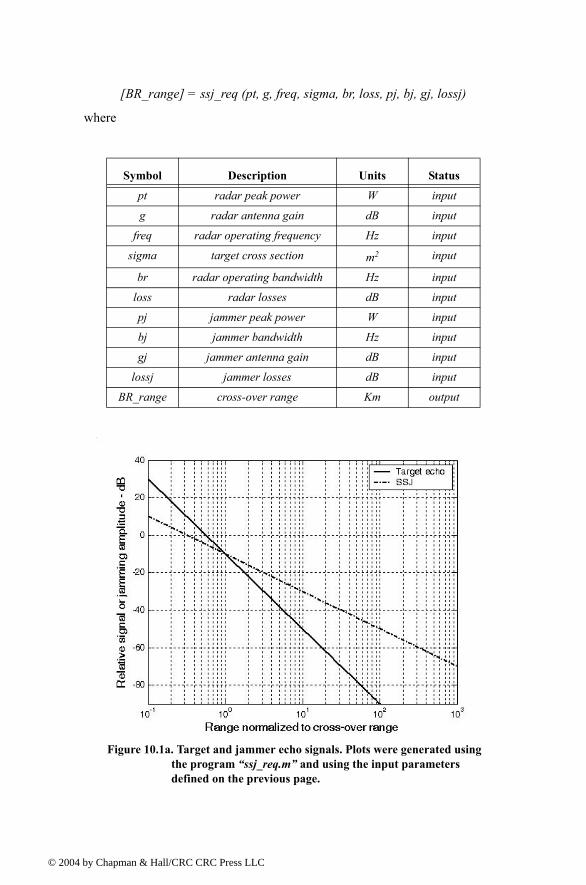
© 200
[BR_range] = ssj_req (pt, g, freq, sigma, br, loss, pj, bj, gj, lossj)
where
Symbol Description Units Status
pt radar peak power W input
g radar antenna gain dB input
freq radar operating frequency Hz input
sigma target cross section m2 input
br radar operating bandwidth Hz input
loss radar losses dB input
pj jammer peak power W input
bj jammer bandwidth Hz input
gj jammer antenna gain dB input
lossj jammer losses dB input
BR_range cross-over range Km output
Figure 10.1a. Target and jammer echo signals. Plots were generated using the program ssj_req.m and using the input parameters defined on the previous page.
4 by Chapman & Hall/CRC CRC Press LLC
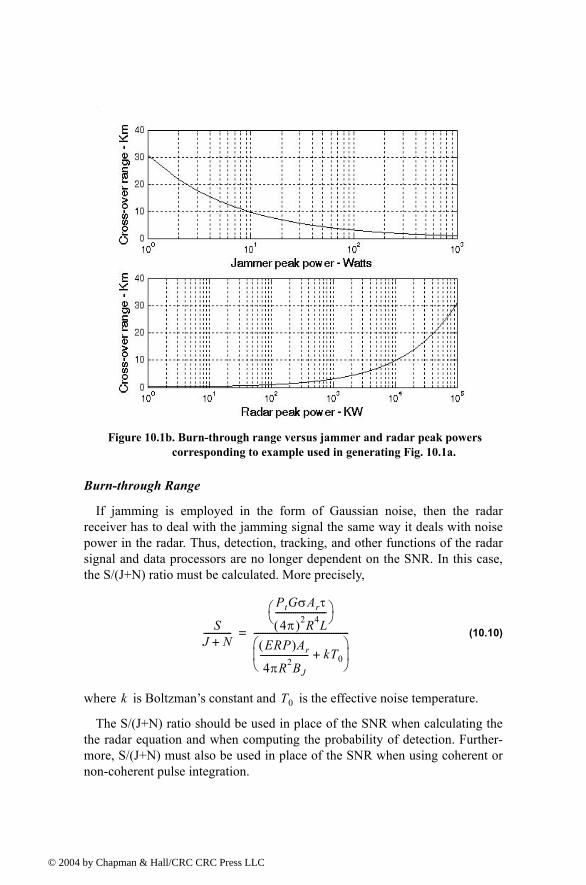
© 200
Burn-through Range
If jamming is employed in the form of Gaussian noise, then the radar receiver has to deal with the jamming signal the same way it deals with noise power in the radar. Thus, detection, tracking, and other functions of the radar signal and data processors are no longer dependent on the SNR. In this case, the S/(J+N) ratio must be calculated. More precisely,
(10.10)
where is Boltzmans constant and is the effective noise temperature.
The S/(J+N) ratio should be used in place of the SNR when calculating the the radar equation and when computing the probability of detection. Further-more, S/(J+N) must also be used in place of the SNR when using coherent or non-coherent pulse integration.
Figure 10.1b. Burn-through range versus jammer and radar peak powers corresponding to example used in generating Fig. 10.1a.
SJ N+-------------
PtGσArτ
4π( )2R4L-----------------------
ERP( )Ar
4πR2BJ
---------------------- kT0+ -------------------------------------------=
k T0
4 by Chapman & Hall/CRC CRC Press LLC
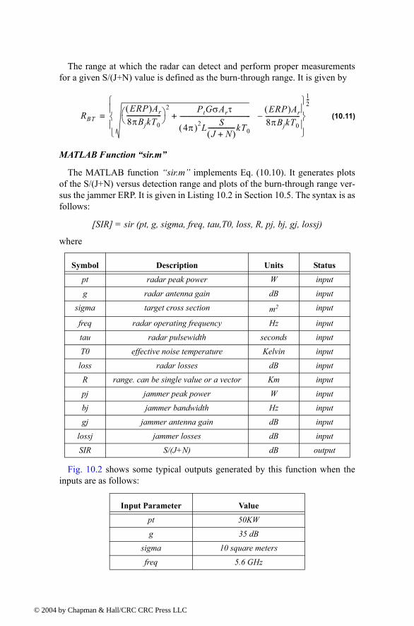
© 200
The range at which the radar can detect and perform proper measurements for a given S/(J+N) value is defined as the burn-through range. It is given by
(10.11)
MATLAB Function sir.m
The MATLAB function sir.m implements Eq. (10.10). It generates plots of the S/(J+N) versus detection range and plots of the burn-through range ver-sus the jammer ERP. It is given in Listing 10.2 in Section 10.5. The syntax is as follows:
[SIR] = sir (pt, g, sigma, freq, tau,T0, loss, R, pj, bj, gj, lossj)
where
Fig. 10.2 shows some typical outputs generated by this function when the inputs are as follows:
Symbol Description Units Status
pt radar peak power W input
g radar antenna gain dB input
sigma target cross section m2 input
freq radar operating frequency Hz input
tau radar pulsewidth seconds input
T0 effective noise temperature Kelvin input
loss radar losses dB input
R range. can be single value or a vector Km input
pj jammer peak power W input
bj jammer bandwidth Hz input
gj jammer antenna gain dB input
lossj jammer losses dB input
SIR S/(J+N) dB output
Input Parameter Value
pt 50KW
g 35 dB
sigma 10 square meters
freq 5.6 GHz
RBTERP( )Ar
8πBjkT0----------------------
2 PtGσArτ
4π( )2L SJ N+( )
-----------------kT0
---------------------------------------------+ERP( )Ar
8πBjkT0----------------------
12---
=
4 by Chapman & Hall/CRC CRC Press LLC
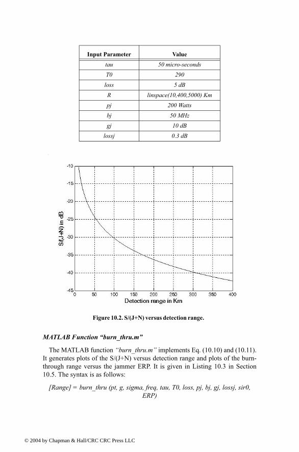
© 200
MATLAB Function burn_thru.m
The MATLAB function burn_thru.m implements Eq. (10.10) and (10.11). It generates plots of the S/(J+N) versus detection range and plots of the burn-through range versus the jammer ERP. It is given in Listing 10.3 in Section 10.5. The syntax is as follows:
[Range] = burn_thru (pt, g, sigma, freq, tau, T0, loss, pj, bj, gj, lossj, sir0, ERP)
tau 50 micro-seconds
T0 290
loss 5 dB
R linspace(10,400,5000) Km
pj 200 Watts
bj 50 MHz
gj 10 dB
lossj 0.3 dB
Input Parameter Value
Figure 10.2. S/(J+N) versus detection range.
4 by Chapman & Hall/CRC CRC Press LLC
© 200
where
Fig. 10.3 shows some typical outputs generated by this function when the inputs are as follows:
Symbol Description Units Status
pt radar peak power W input
g radar antenna gain dB input
sigma target cross section m2 input
freq radar operating frequency Hz input
tau radar pulsewidth seconds input
T0 effective noise temperature Kelvin input
loss radar losses dB input
pj jammer peak power W input
bj jammer bandwidth Hz input
gj jammer antenna gain dB input
lossj jammer losses dB input
sir0 desired SIR dB input
ERP desired ERP. can be a vector Watts input
Range burn-through range Km output
Input Parameter Value
pt 50KW
g 35 dB
sigma 10 square meters
freq 5.6 GHz
tau 0.5 milli-seconds
T0 290
loss 5 dB
pj 200 Watts
bj 500 MHz
gj 10 dB
lossj 0.3 dB
sir0 15dB
ERP linspace(1, 1000, 1000) W
4 by Chapman & Hall/CRC CRC Press LLC
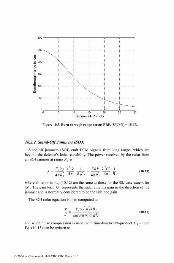
© 200
10.2.2. Stand-Off Jammers (SOJ)
Stand-off jammers (SOJ) emit ECM signals from long ranges which are beyond the defenses lethal capability. The power received by the radar from an SOJ jammer at range is
(10.12)
where all terms in Eq. (10.12) are the same as those for the SSJ case except for . The gain term represents the radar antenna gain in the direction of the
jammer and is normally considered to be the sidelobe gain.
The SOJ radar equation is then computed as
(10.13)
and when pulse compression is used, with time-bandwidth-product then Eq. (10.13) can be written as
Figure 10.3. Burn-through range versus ERP. (S/(J+N) = 15 dB.
RJ
JPJGJ
4πRJ2
------------- λ2G′4π
------------ 1BJLJ----------- ERP
4πRJ2
------------- λ2G′4π
------------ 1BJ-----= =
G′ G′
SJ---
PtτG2RJ2σBJ
4π ERP( )G′R4L----------------------------------------=
GPC
4 by Chapman & Hall/CRC CRC Press LLC
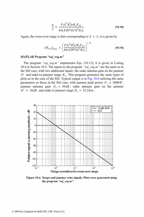
© 200
(10.14)
Again, the cross-over range is that corresponding to ; it is given by
(10.15)
MATLAB Program soj_req.m
The program soj_req.m implements Eqs. (10.15); it is given in Listing 10.4 in Section 10.5. The inputs to the program soj_req.m are the same as in the SSJ case, with two additional inputs: the radar antenna gain on the jammer
and radar-to-jammer range . This program generates the same types of plots as in the case of the SSJ. Typical output is in Fig. 10.4 utilizing the same parameters as those in the SSJ case, with jammer peak power , jammer antenna gain , radar antenna gain on the jammer
, and radar to jammer range .
SJ---
PtG2RJ
2σBJPPC
4π ERP( )G′R4BrL----------------------------------------------=
S J=
RCO( )SOJPtG
2RJ2σBJPPC
4π ERP( )G′BrL---------------------------------------
1 4⁄
=
G′ RJ
PJ 5000W=GJ 30dB=
G′ 10dB= RJ 22.2Km=
Figure 10.4. Target and jammer echo signals. Plots were generated using the program soj_req.m.
4 by Chapman & Hall/CRC CRC Press LLC
© 200
Again if the jamming is employed in the form of Gaussian noise, then the radar receiver has to deal with the jamming signal the same way it deals with noise power in the radar. In this case, the S/(J+N) is
(10.16)
10.3. Range Reduction FactorConsider a radar system whose detection range in the absence of jamming
is governed by
(10.17)
The term Range Reduction Factor (RRF) refers to the reduction in the radar detection range due to jamming. More precisely, in the presence of jamming the effective radar detection range is
(10.18)
In order to compute RRF, consider a radar characterized by Eq. (10.17), and a barrage jammer whose output power spectral density is (i.e., Gaussian-like). Then the amount of jammer power in the radar receiver is
(10.19)
where is the jammer effective temperature. It follows that the total jammer plus noise power in the radar receiver is given by
(10.20)
In this case, the radar detection range is now limited by the receiver signal-to-noise plus interference ratio rather than SNR. More precisely,
(10.21)
The amount of reduction in the signal-to-noise plus interference ratio because of the jammer effect can be computed from the difference between Eqs. (10.17) and (10.21). It is expressed (in dB) by
SJ N+-------------
PtGσArτ
4π( )2R4L-----------------------
ERP( )ArG'
4πRJ2BJ
---------------------------- kT0+ -------------------------------------------------=
R
SNR( )oPtG
2λ2σ
4π( )3kTeBrFLR4------------------------------------------=
Rdj R RRF×=
Jo
J kTJBr=
TJ
Ni J+ kTeBr kTJBr+=
SJ N+------------- PtG
2λ2σ
4π( )3k Te TJ+( )BrFLR4-----------------------------------------------------------=
4 by Chapman & Hall/CRC CRC Press LLC
© 200
(10.22)
Consequently, the RRF is
(10.23)
MATLAB Function range_red_factor.m
The function range_red_factor.m implements Eqs. (10.22) and (10.23); it is given in Listing 10.5 in Section 10.5. This function generates plots of RRF versus: (1) the radar operating frequency; (2) radar to jammer range; and (3) jammer power. Its syntax is as follows:
[RRF] = range_red_factor (te, pj, gj, g, freq, bj, rangej, lossj)
where
The following values were used to produce Figs. 10.5 through 10.7.
Symbol Description Units Status
te radar effective temperature K input
pj jammer peak power W input
gj jammer antenna gain dB input
g radar antenna gain on jammer dB input
freq radar operating frequency Hz input
bj jammer bandwidth Hz input
rangej radar to jammer range Km input
lossj jammer losses dB input
Symbol Value
te 500 kelvin
pj 500 KW
gj 3 dB
g 45 dB
freq 10 GHz
bj 10 MHZ
rangej 750 Km
lossj 1 dB
ϒ 10.0 1TJ
Te-----+
log×=
RRF 10ϒ
40------
=
4 by Chapman & Hall/CRC CRC Press LLC
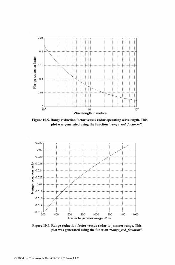
© 200
Figure 10.5. Range reduction factor versus radar operating wavelength. This plot was generated using the function range_red_factor.m.
Figure 10.6. Range reduction factor versus radar to jammer range. This plot was generated using the function range_red_factor.m.
4 by Chapman & Hall/CRC CRC Press LLC
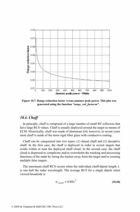
© 200
10.4. ChaffIn principle, chaff is composed of a large number of small RF reflectors that
have large RCS values. Chaff is usually deployed around the target as means of ECM. Historically, chaff was made of aluminum foil; however, in recent years most chaff is made of the more rigid fiber glass with conductive coating.
Chaff can be categorized into two types: (1) denial chaff and (2) deceptive chaff. In the first case, the chaff is deployed in order to screen targets that reside within or near the deployed chaff cloud. In the second case, the chaff cloud is dispersed to complicate and/or overwhelm the tracking and processing functions of the radar by luring the tracker away from the target and/or creating multiple false targets.
The maximum chaff RCS occurs when the individual chaff-dipole length is one half the radar wavelength. The average RCS for a single dipole when viewed broadside is
(10.24)
Figure 10.7. Range reduction factor versus jammer peak power. This plot was generated using the function range_red_factor.m.
L
σchaff1 0.88λ2≈
4 by Chapman & Hall/CRC CRC Press LLC
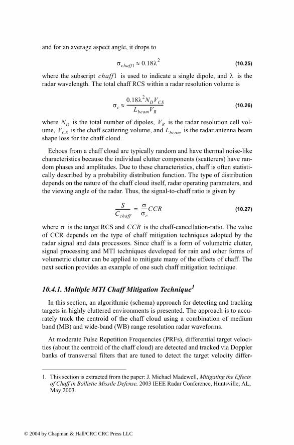
© 200
and for an average aspect angle, it drops to
(10.25)
where the subscript is used to indicate a single dipole, and is the radar wavelength. The total chaff RCS within a radar resolution volume is
(10.26)
where is the total number of dipoles, is the radar resolution cell vol-ume, is the chaff scattering volume, and is the radar antenna beam shape loss for the chaff cloud.
Echoes from a chaff cloud are typically random and have thermal noise-like characteristics because the individual clutter components (scatterers) have ran-dom phases and amplitudes. Due to these characteristics, chaff is often statisti-cally described by a probability distribution function. The type of distribution depends on the nature of the chaff cloud itself, radar operating parameters, and the viewing angle of the radar. Thus, the signal-to-chaff ratio is given by
(10.27)
where is the target RCS and is the chaff-cancellation-ratio. The value of CCR depends on the type of chaff mitigation techniques adopted by the radar signal and data processors. Since chaff is a form of volumetric clutter, signal processing and MTI techniques developed for rain and other forms of volumetric clutter can be applied to mitigate many of the effects of chaff. The next section provides an example of one such chaff mitigation technique.
10.4.1. Multiple MTI Chaff Mitigation Technique1
In this section, an algorithmic (schema) approach for detecting and tracking targets in highly cluttered environments is presented. The approach is to accu-rately track the centroid of the chaff cloud using a combination of medium band (MB) and wide-band (WB) range resolution radar waveforms.
At moderate Pulse Repetition Frequencies (PRFs), differential target veloci-ties (about the centroid of the chaff cloud) are detected and tracked via Doppler banks of transversal filters that are tuned to detect the target velocity differ-
1. This section is extracted from the paper: J. Michael Madewell, Mitigating the Effects of Chaff in Ballistic Missile Defense, 2003 IEEE Radar Conference, Huntsville, AL, May 2003.
σchaff1 0.18λ2≈
chaff1 λ
σc0.18λ2NDVCS
LbeamVR---------------------------------≈
ND VRVCS Lbeam
SCchaff------------- σ
σc-----CCR=
σ CCR
4 by Chapman & Hall/CRC CRC Press LLC
© 200
ences. Through sensitivity analysis models, the theoretical lower bound on detectable differential target velocity as a function of the chaff cloud composi-tion (e.g., clutter cross section, clutter spectral width, number of dipoles, and clutter velocity standard deviation) and radar related parameters (e.g., wave-form frequency, bandwidth, integration times, PRFs, and signal-to-clutter ratio) are analyzed.
Overview
A five-step approach for detecting and tracking targets in highly cluttered environments has been developed. The five steps are:
1. Utilize a 1 to 5 percent MB bandwidth, high PRF radar waveform, to mea-sure the chaff cloud range extent, centroid, and velocity growth rate.
2. Establish track on the centroid of the chaff cloud with the MB waveform. 3. Based on course track information obtained in steps 1) and 2), implement
WB track (10% or greater bandwidth waveform) on the cloud centroid.4. Design a doppler bank of Moving Target Indicator (MTI) transversal filters
to provide adequate gain at specific velocity increments about the WB cen-troid track.
5. Process the Multiple MTI (M2) doppler filters in parallel to detect differ-ences in target Doppler (with respect to the cloud centroid track velocity). Targets are detected when integration at the correct Doppler difference occurs.
Operational concerns that have been identified for implementation of this approach include: (1) the ability of a radar to adequately track the centroid of the chaff cloud (i.e., track precision); (2) the ability of a radar to detect small differences in target Doppler relative to the chaff cloud centroid (i.e., Doppler precision); and (3) the ability of a filter (in this case, a bank of MTI's) to achieve the necessary processing gain to detect the target
Theoretical tracking accuracy of a chaff cloud
The single pulse thermal-noise error in a velocity tracking measurement for optimum processing can be described by
(10.28)
where is the pulsewidth and is that for the target in track. To detect tar-gets in clutter, substitute the difference-channel chaff-to-signal ratio for . More precisely,
(10.29)
σf
σf1
1.81τ 2 SNR×--------------------------------------=
τ SNRSNR
σf1
1.81τ 2 Cchaff S⁄×------------------------------------------------=
4 by Chapman & Hall/CRC CRC Press LLC
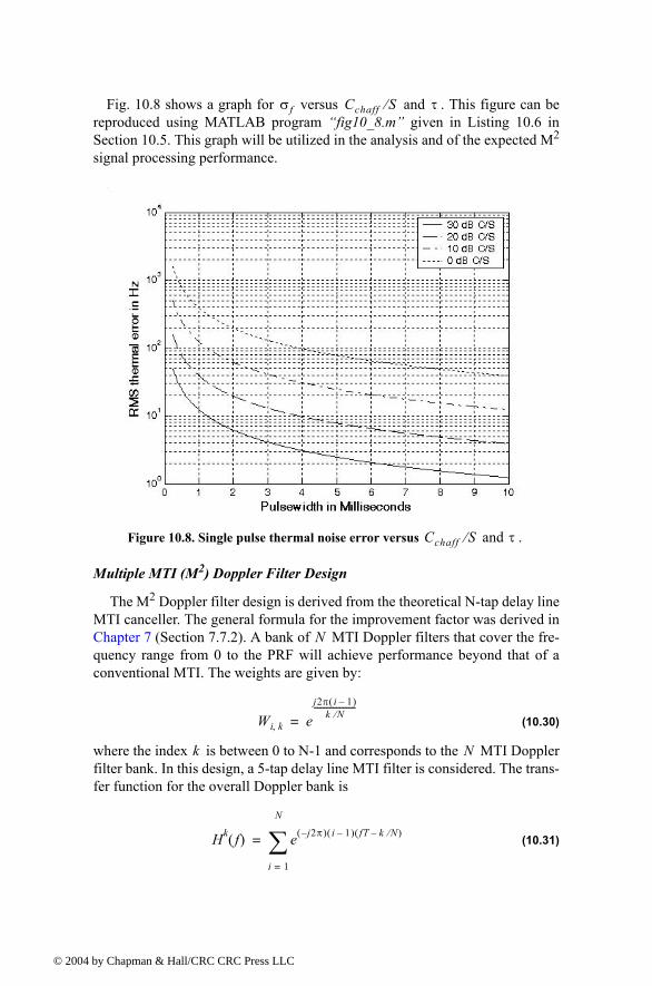
© 200
Fig. 10.8 shows a graph for versus and . This figure can be reproduced using MATLAB program fig10_8.m given in Listing 10.6 in Section 10.5. This graph will be utilized in the analysis and of the expected M2
signal processing performance.
Multiple MTI (M2) Doppler Filter Design
The M2 Doppler filter design is derived from the theoretical N-tap delay line MTI canceller. The general formula for the improvement factor was derived in Chapter 7 (Section 7.7.2). A bank of MTI Doppler filters that cover the fre-quency range from 0 to the PRF will achieve performance beyond that of a conventional MTI. The weights are given by:
(10.30)
where the index is between 0 to N-1 and corresponds to the MTI Doppler filter bank. In this design, a 5-tap delay line MTI filter is considered. The trans-fer function for the overall Doppler bank is
(10.31)
σf Cchaff S⁄ τ
Figure 10.8. Single pulse thermal noise error versus and .Cchaff S⁄ τ
N
Wi k, ej2π i 1( )
k N⁄------------------------
=
k N
Hk f( ) e j2π( ) i 1( ) fT k N⁄( )
i 1=
N
∑=
4 by Chapman & Hall/CRC CRC Press LLC
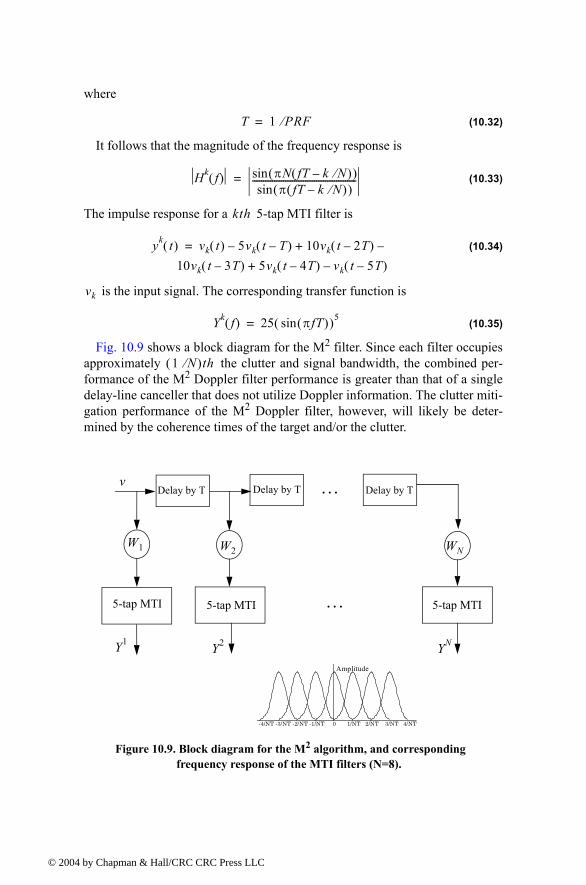
© 200
where
(10.32)
It follows that the magnitude of the frequency response is
(10.33)
The impulse response for a 5-tap MTI filter is
(10.34)
is the input signal. The corresponding transfer function is
(10.35)
Fig. 10.9 shows a block diagram for the M2 filter. Since each filter occupies approximately the clutter and signal bandwidth, the combined per-formance of the M2 Doppler filter performance is greater than that of a single delay-line canceller that does not utilize Doppler information. The clutter miti-gation performance of the M2 Doppler filter, however, will likely be deter-mined by the coherence times of the target and/or the clutter.
T 1 PRF⁄=
Hk f( ) πN fT k N⁄( )( )sinπ fT k N⁄( )( )sin
-----------------------------------------------=
kth
yk t( ) vk t( ) 5vk t T( ) 10vk t 2T( )10vk t 3T( )
5vk t 4T( ) vk t 5T( )
+
+
=
vk
Yk f( ) 25 πfT( )sin( )5=
1 N⁄( )th
…Delay by T Delay by T Delay by T
5-tap MTI 5-tap MTI 5-tap MTI
W1
Y1 Y2
WNW2
YN
Amplitude
-4/NT -3/NT -2/NT -1/NT 0 1/NT 2/NT 3/NT 4/NT
Figure 10.9. Block diagram for the M2 algorithm, and corresponding frequency response of the MTI filters (N=8).
…
v
4 by Chapman & Hall/CRC CRC Press LLC
© 200
Processor Implementation And Simulated Results
The M2 filter approach outlined in this section requires a very accurate track of the centroid of the chaff cloud being probed. As described earlier, initiation of track on the chaff cloud centroid is achieved with a MB range resolution waveform (step 1). As an example, assume that an X-band radar (10 GHz) is engaging one or more ballistic targets enveloped in a chaff cloud that contains 1 million dipoles occupying a 1-kilometer range extent. Assuming that the chaff cloud velocity distribution can be accurately modeled by Gaussian statis-tics, approximately 67% of these dipoles will reside in 333 meters of range extent. With these assumptions, the combined average RCS of the dipoles ( ) contained within a radar range resolution cell of this length (333 m) can be approximated by
(10.36)
The RCS of a typical ballistic Reentry Vehicle (RV) at forward aspect view-ing angles can be or smaller. Therefore, the MB for a typ-ical RV enveloped by the chaff cloud assumed above can approach or greater. Using an 8-msec pulsewidth and , the theoretical, sin-gle pulse, minimum rms track error is approximately . At X-band frequencies, this translates to a single pulse velocity error of
(10.37)
Note that for a train of pulses, this velocity error can be reduced by a factor of 10 or more. Thus, for a typical X-band radar, theory suggests that the track pre-cision of the chaff cloud centroid can approach 0.0015 m/s or better. This track precision is much less than the WB range resolution capability of the radar and therefore can be utilized to bootstrap the WB tracker (steps 2 and 3).
Assume a Gaussian chaff clutter velocity distribution and denote it . If ( relative to the cloud centroid velocity), the mini-
mum PRF required to meet the Nyquist sampling criterion is
(10.38)
Also, assume that a bank of Doppler MTI's (step 4) can be formed to cover this frequency range. Note that 256 is the closest 2N multiple for implementation with the Fast Fourier Transform (FFT). Using a 256 point FFT design, each fil-ter will contain approximately 1/256 of the total clutter velocities (about 0.03 m/s of velocity clutter per MTI Doppler filter). In addition, by utilizing the WB track waveform, a very precise range-Doppler image can be formed (with each range-Doppler resolution cell containing approximately 15 cm by 0.03 m/s of
RCSD
RCSD 0.18NDλ2 0.18 670 000, 0.032×× 108.54= = = 20.4dBsm⇒
20dBsm Cchaff S⁄40dB
30dB Cchaff S⁄fe 1Hz=
vefeλ2
------- 0.015m s⁄= =
vgvg 1.8m s⁄= 0.9m s⁄±
PRF fr 22vg
λ--------×≥ 240Hz= =
4 by Chapman & Hall/CRC CRC Press LLC
© 200
clutter). This design effectively reduces the amount of clutter that competes with an individual target scatter by a factor of more than 40 dB, thus reducing the by this same amount.
For extreme chaff cases where the initial WB range-Doppler image S/C is negative, an N-pulse coherent sliding window routine can be applied to the data prior to implementing the M2 algorithm. For example, a 16 pulse coherent sliding window can provide up to 12 dB of improvement. One should ensure that the number of pulses integrated is less than the coherency time of the target and clutter. Other constraints in implementing this approach are to ensure that the target phase does not deviate very much during the inte-gration period (to ensure optimum coherent processing gain) and the target position does not migrate to another range and/or Doppler cell (often referred to as range-Doppler walk). The zero Doppler filter (and/or near zero Doppler filters) can be used to perform statistics on the clutter and to adaptively adjust the optimal threshold setting to obtain low false alarms and high probabilities of detection over time.
A model for the M2 signal processor has been developed using MATLAB. Fig. 10.10 shows a plot of the amplitude versus range and Doppler (256x256 range-Doppler image) of three constant -20 dBsm target scatterers that are embedded in approximately -15 dBsm Gaussian white noise. In this figure, the noise completely envelops the signal. These modeling results are comparable to the output of a typical range Doppler imaging radar. Fig. 10.11 shows the results obtained by executing the first two blocks of the M2 signal processor. As expected, the three scatterers rise from above the noise and now have an
ratio of approximately 7 dB.
Finally, Fig. 10.12 shows the results obtained by implementing the entire top portion of the M2 signal processing chain. No attempt was made to optimize the threshold level. Instead, the threshold was manually set to -43 dB to allow for some of the higher false alarms to be seen in the figure. The largest ampli-tude false alarms are approximately -34 dB. Meanwhile, the amplitudes of the target returns have been reduced (less than 1 dB) from that of Fig. 10.11. Therefore, the improvement in Fig. 10.12 over that shown in Fig. 10.11 is approximately 8 to 9 dB. Hence, the processing gain attributed to the M2 signal processor is more than 20 dB above that of traditional range Doppler processing.
In summary, one concludes that the M2 signal processing algorithm for detecting and tracking ballistic missile targets in highly cluttered environments can provide better than 20 dB improvement over that of traditional range Doppler processing techniques alone.
Cchaff S⁄
S Cchaff⁄
S Cchaff⁄
S Cchaff⁄
S Cchaff⁄
4 by Chapman & Hall/CRC CRC Press LLC
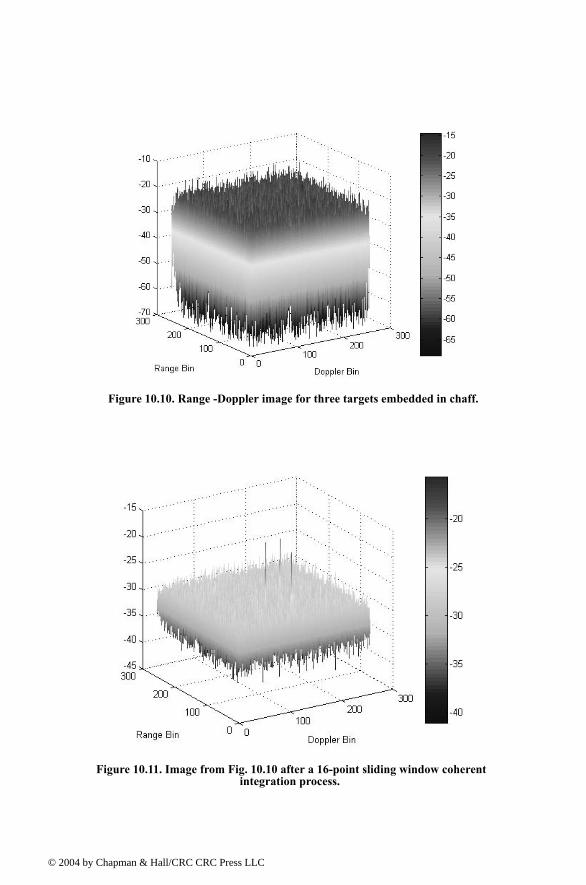
© 200
Figure 10.10. Range -Doppler image for three targets embedded in chaff.
Figure 10.11. Image from Fig. 10.10 after a 16-point sliding window coherent integration process.
4 by Chapman & Hall/CRC CRC Press LLC
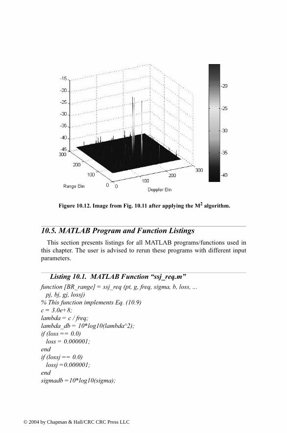
© 200
10.5. MATLAB Program and Function ListingsThis section presents listings for all MATLAB programs/functions used in
this chapter. The user is advised to rerun these programs with different input parameters.
Listing 10.1. MATLAB Function ssj_req.mfunction [BR_range] = ssj_req (pt, g, freq, sigma, b, loss, ... pj, bj, gj, lossj)% This function implements Eq. (10.9)c = 3.0e+8;lambda = c / freq;lambda_db = 10*log10(lambda^2);if (loss == 0.0) loss = 0.000001;endif (lossj == 0.0) lossj =0.000001;endsigmadb =10*log10(sigma);
Figure 10.12. Image from Fig. 10.11 after applying the M2 algorithm.
4 by Chapman & Hall/CRC CRC Press LLC
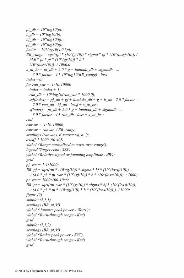
© 200
pt_db = 10*log10(pt);b_db = 10*log10(b);bj_db = 10*log10(bj);pj_db = 10*log10(pj);factor = 10*log10(4.0 *pi);BR_range = sqrt((pt * (10^(g/10)) * sigma * bj * (10^(lossj/10))) / ... (4.0 * pi * pj * (10^(gj/10)) * b * ... (10^(loss/10)))) / 1000.0 s_at_br = pt_db + 2.0 * g + lambda_db + sigmadb - ... 3.0 * factor - 4.* 10*log10(BR_range) - loss index =0;for ran_var = .1:10:10000 index = index + 1; ran_db = 10*log10(ran_var * 1000.0); ssj(index) = pj_db + gj + lambda_db + g + b_db - 2.0 * factor - ... 2.0 * ran_db - bj_db - lossj + s_at_br ; s(index) = pt_db + 2.0 * g + lambda_db + sigmadb - ... 3.0 * factor - 4.* ran_db - loss + s_at_br ;endranvar = .1:10:10000;ranvar = ranvar ./ BR_range;semilogx (ranvar,s,'k',ranvar,ssj,'k-.');axis([.1 1000 -90 40])xlabel ('Range normalized to cross-over range');legend('Target echo','SSJ')ylabel ('Relative signal or jamming amplitude - dB');gridpj_var = 1:1:1000;BR_pj = sqrt((pt * (10^(g/10)) * sigma * bj * (10^(lossj/10))) ... ./ (4.0 * pi .* pj_var * (10^(gj/10)) * b * (10^(loss/10)))) ./ 1000;pt_var = 1000:100:10e6;BR_pt = sqrt((pt_var * (10^(g/10)) * sigma * bj * (10^(lossj/10))) ... ./ (4.0 * pi .* pj * (10^(gj/10)) * b * (10^(loss/10)))) ./ 1000;figure (2)subplot (2,1,1)semilogx (BR_pj,'k')xlabel ('Jammer peak power - Watts');ylabel ('Burn-through range - Km')gridsubplot (2,1,2)semilogx (BR_pt,'k')xlabel ('Radar peak power - KW')ylabel ('Burn-through range - Km')grid
4 by Chapman & Hall/CRC CRC Press LLC
© 200
Listing 10.2. MATLAB Function sir.mfunction [SIR] = sir (pt, g, freq, sigma, tau,T0, loss, R, pj, bj, gj, lossj);c = 3.0e+8;k = 1.38e-23;%R = linspace(rmin, rmax, 1000);range = R .* 1000;lambda = c / freq;gj = 10^(gj/10);G = 10^(g/10);ERP1 = pj * gj / lossj;ERP_db = 10*log10(ERP1);% Calculate Eq. (10.10)Ar = lambda *lambda * G / 4 /pi;num1 = pt * tau * G * sigma * Ar;demo1 = 4^2 * pi^2 * loss .* range.^4;demo2 = 4 * pi * bj .* range.^2;num2 = ERP1 * Ar;val11 = num1 ./ demo1;val21 = num2 ./demo2; sir = val11 ./ (val21 + k * T0);SIR = 10*log10(sir);figure (1)plot (R, SIR,'k')xlabel ('Detection range in Km');ylabel ('S/(J+N) in dB')grid
Listing 10.3. MATLAB Function burn_thru.mfunction [Range] = burn_thru (pt, g, freq, sigma, tau, T0, loss, pj, bj, gj, lossj,sir0,ERP);c = 3.0e+8;k = 1.38e-23;%R = linspace(rmin, rmax, 1000);sir0 = 10^(sir0/10);lambda = c / freq;gj = 10^(gj/10);G = 10^(g/10); Ar = lambda *lambda * G / 4 /pi;%ERP = linspace(1,1000,5001);num32 = ERP .* Ar;demo3 = 8 *pi * bj * k * T0;demo4 = 4^2 * pi^2 * k * T0 * sir0;
4 by Chapman & Hall/CRC CRC Press LLC
© 200
val1 = (num32 ./ demo3).^2;val2 = (pt * tau * G * sigma * Ar)/(4^2 * pi^2 * loss * sir0 * k *T0);val3 = sqrt(val1 + val2);val4 = (ERP .* Ar) ./ demo3;Range = sqrt(val3 - val4) ./ 1000;figure (1)plot (10*log10(ERP), Range,'k')xlabel (' Jammer ERP in dB')ylabel ('Burnthrough range in Km')grid
Listing 10.4. MATLAB Function soj_req.mfunction [BR_range] = soj_req (pt, g, sigma, b, freq, loss, range, ... pj, bj,gj, lossj, gprime, rangej)% This function implements equations for SOJsc = 3.0e+8;lambda = c / freq;lambda_db = 10*log10(lambda^2)if (loss == 0.0) loss = 0.000001;endif (lossj == 0.0) lossj =0.000001;endsigmadb = 10*log10(sigma);range_db = 10*log10(range * 1000.);rangej_db = 10*log10(rangej * 1000.)pt_db = 10*log10(pt);b_db = 10*log10(b);bj_db = 10*log10(bj);pj_db = 10*log10(pj);factor = 10*log10(4.0 *pi);BR_range = ((pt * 10^(2.0*g/10) * sigma * bj * 10^(lossj/10) * ... (rangej)^2) / (4.0 * pi * pj * 10^(gj/10) * 10^(gprime/10) * ... b * 10^(loss/10)))^.25 / 1000. s_at_br = pt_db + 2.0 * g + lambda_db + sigmadb - ... 3.0 * factor - 4.0 * 10*log10(BR_range) - loss index =0;for ran_var = .1:1:1000; index = index + 1; ran_db = 10*log10(ran_var * 1000.0); s(index) = pt_db + 2.0 * g + lambda_db + sigmadb - ... 3.0 * factor - 4.0 * ran_db - loss + s_at_br;
4 by Chapman & Hall/CRC CRC Press LLC
© 200
soj(index) = s_at_br - s_at_br;endranvar = .1:1:1000;%ranvar = ranvar ./BR_range;semilogx (ranvar,s,'k',ranvar,soj,'k-.');xlabel ('Range normalized to cross-over range');legend('Target echo','SOJ')ylabel ('Relative signal or jamming amplitude - dB');
Listing 10.5. MATLAB Function range_red_factor.mfunction RRF = range_red_factor (te, pj, gj, g, freq, bj, rangej, lossj)% This function computes the range reduction factor and produces% plots of RRF versus wavelength, radar to jammer range, and jammer power c = 3.0e+8;k = 1.38e-23;lambda = c / freq;gj_10 = 10^( gj/10);g_10 = 10^( g/10);lossj_10 = 10^(lossj/10);index = 0;for wavelength = .01:.001:1 index = index +1; jamer_temp = (pj * gj_10 * g_10 *wavelength^2) / ... (4.0^2 * pi^2 * k * bj * lossj_10 * (rangej * 1000.0)^2); delta = 10.0 * log10(1.0 + (jamer_temp / te)); rrf(index) = 10^(-delta /40.0); endw = 0.01:.001:1;figure (1)semilogx(w,rrf,'k')gridxlabel ('Wavelength in meters')ylabel ('Range reduction factor')index = 0;for ran =rangej*.3:1:rangej*2 index = index + 1; jamer_temp = (pj * gj_10 * g_10 *wavelength^2) / ... (4.0^2 * pi^2 * k * bj * lossj_10 * (ran * 1000.0)^2); delta = 10.0 * log10(1.0 + (jamer_temp / te)); rrf1(index) = 10^(-delta /40.0);endfigure(2)ranvar = rangej*.3:1:rangej*2 ;
4 by Chapman & Hall/CRC CRC Press LLC
© 200
plot(ranvar,rrf1,'k')gridxlabel ('Radar to jammer range - Km')ylabel ('Range reduction factor')index = 0;for pjvar = pj*.01:1:pj*2 index = index + 1; jamer_temp = (pjvar * gj_10 * g_10 *wavelength^2) / ... (4.0^2 * pi^2 * k * bj * lossj_10 * (rangej * 1000.0)^2); delta = 10.0 * log10(1.0 + (jamer_temp / te)); rrf2(index) = 10^(-delta /40.0);endfigure(3)pjvar = pj*.01:1:pj*2;plot(pjvar,rrf2,'k')gridxlabel ('Jammer peak power - Watts')ylabel ('Range reduction factor')%%%%%%%%%%%%%%%%%%%%%%%%%%%%%%%% Use this input file to reproduce Figs. 10.5 through 10.7clear allte = 500.0; % radar effective temp. in Kelvinpj= 500; % jammer peak power in Wgj = 3.0; % jammer antenna gain in dBg = 45.0; % radar antenna gainfreq = 10.0e+9;% radar operating frequency in Hzbj= 10.0e+6; % radar operating bandwidth in Hzrangej = 750.0;% radar to jammer range in Kmlossj = 1.0; % jammer losses in dB
Listing 10.6. MATLAB Program fig10_8.m% Use this program to reproduce Fig. 10.8 in the textclear allclose alltau = linspace(.25,10,500);taum = tau .* 1e-3;C_S = [-20 -10 0 10];c_s = 10.^(C_S./10);for n = 1:size(C_S,2) val1 = 1 / (1.81*sqrt(2*c_s(n))); sigma(n,:) = val1 ./ taum;endfigure (1)
4 by Chapman & Hall/CRC CRC Press LLC

© 200
semilogy(tau,sigma(1,:),'k',tau,sigma(2,:),'k-- ',tau,sigma(3,:),'k-.', ... tau,sigma(4,:),'k:');xlabel('Pulsewidth in Milliseconds')ylabel('RMS thermal error in Hz')legend('-20 dB C/S','-10 dB C/S','0 dB C/S','10 dB C/S')grid
4 by Chapman & Hall/CRC CRC Press LLC
© 200
Chapter 11 Radar Cross Section (RCS)
In this chapter, the phenomenon of target scattering and methods of RCScalculation are examined. Target RCS fluctuations due to aspect angle, fre-quency, and polarization are presented. Radar cross section characteristics ofsome simple and complex targets are also introduced.
11.1. RCS DefinitionElectromagnetic waves, with any specified polarization, are normally dif-
fracted or scattered in all directions when incident on a target. These scatteredwaves are broken down into two parts. The first part is made of waves thathave the same polarization as the receiving antenna. The other portion of thescattered waves will have a different polarization to which the receivingantenna does not respond. The two polarizations are orthogonal and arereferred to as the Principal Polarization (PP) and Orthogonal Polarization(OP), respectively. The intensity of the backscattered energy that has the samepolarization as the radars receiving antenna is used to define the target RCS.When a target is illuminated by RF energy, it acts like an antenna, and willhave near and far fields. Waves reflected and measured in the near field are, ingeneral, spherical. Alternatively, in the far field the wavefronts are decom-posed into a linear combination of plane waves.
Assume the power density of a wave incident on a target located at range away from the radar is , as illustrated in Fig. 11.1. The amount of reflectedpower from the target is
(11.1)
RPDi
Pr σPDi=
4 by Chapman & Hall/CRC CRC Press LLC
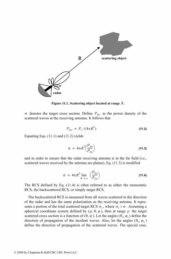
© 200
denotes the target cross section. Define as the power density of thescattered waves at the receiving antenna. It follows that
(11.2)
Equating Eqs. (11.1) and (11.2) yields
(11.3)
and in order to ensure that the radar receiving antenna is in the far field (i.e.,scattered waves received by the antenna are planar), Eq. (11.3) is modified
(11.4)
The RCS defined by Eq. (11.4) is often referred to as either the monostaticRCS, the backscattered RCS, or simply target RCS.
The backscattered RCS is measured from all waves scattered in the directionof the radar and has the same polarization as the receiving antenna. It repre-sents a portion of the total scattered target RCS , where . Assuming aspherical coordinate system defined by ( ), then at range the targetscattered cross section is a function of ( ). Let the angles ( ) define thedirection of propagation of the incident waves. Also, let the angles ( )define the direction of propagation of the scattered waves. The special case,
Figure 11.1. Scattering object located at range .R
Radar
R
Radar
R scattering object
radar
σ PDr
PDr Pr 4πR2( )⁄=
σ 4πR2 PDr
PDi-------- =
σ 4πR2 PDr
PDi--------
R ∞→lim=
σt σt σ>ρ θ ϕ, , ρ
θ ϕ, θi ϕi,θs ϕs,
4 by Chapman & Hall/CRC CRC Press LLC
© 200
when and , defines the monostatic RCS. The RCS measuredby the radar at angles and is called the bistatic RCS.
The total target scattered RCS is given by
(11.5)
The amount of backscattered waves from a target is proportional to the ratioof the target extent (size) to the wavelength, , of the incident waves. In fact, aradar will not be able to detect targets much smaller than its operating wave-length. For example, if weather radars use L-band frequency, rain dropsbecome nearly invisible to the radar since they are much smaller than thewavelength. RCS measurements in the frequency region, where the targetextent and the wavelength are comparable, are referred to as the Rayleighregion. Alternatively, the frequency region where the target extent is muchlarger than the radar operating wavelength is referred to as the optical region.In practice, the majority of radar applications fall within the optical region.
The analysis presented in this book mainly assumes far field monostaticRCS measurements in the optical region. Near field RCS, bistatic RCS, andRCS measurements in the Rayleigh region will not be considered since theirtreatment falls beyond this books intended scope. Additionally, RCS treatmentin this chapter is mainly concerned with Narrow Band (NB) cases. In otherwords, the extent of the target under consideration falls within a single rangebin of the radar. Wide Band (WB) RCS measurements will be briefly addressedin a later section. Wide band radar range bins are small (typically 10 - 50 cm);hence, the target under consideration may cover many range bins. The RCSvalue in an individual range bin corresponds to the portion of the target fallingwithin that bin.
11.2. RCS Prediction MethodsBefore presenting the different RCS calculation methods, it is important to
understand the significance of RCS prediction. Most radar systems use RCS asa means of discrimination. Therefore, accurate prediction of target RCS is crit-ical in order to design and develop robust discrimination algorithms. Addition-ally, measuring and identifying the scattering centers (sources) for a giventarget aid in developing RCS reduction techniques. Another reason of lesserimportance is that RCS calculations require broad and extensive technicalknowledge; thus, many scientists and scholars find the subject challenging andintellectually motivating. Two categories of RCS prediction methods are avail-able: exact and approximate.
θs θi= ϕs ϕi=θs θi≠ ϕs ϕi≠
σt1
4π------ σ θs ϕs,( ) θssin θd ϕsd
θs 0=
π
∫ϕs 0=
2π
∫=
λ
4 by Chapman & Hall/CRC CRC Press LLC
© 200
Exact methods of RCS prediction are very complex even for simple shapeobjects. This is because they require solving either differential or integral equa-tions that describe the scattered waves from an object under the proper set ofboundary conditions. Such boundary conditions are governed by Maxwellsequations. Even when exact solutions are achievable, they are often difficult tointerpret and to program using digital computers.
Due to the difficulties associated with the exact RCS prediction, approxi-mate methods become the viable alternative. The majority of the approximatemethods are valid in the optical region, and each has its own strengths and lim-itations. Most approximate methods can predict RCS within few dBs of thetruth. In general, such a variation is quite acceptable by radar engineers anddesigners. Approximate methods are usually the main source for predictingRCS of complex and extended targets such as aircrafts, ships, and missiles.When experimental results are available, they can be used to validate and ver-ify the approximations.
Some of the most commonly used approximate methods are GeometricalOptics (GO), Physical Optics (PO), Geometrical Theory of Diffraction (GTD),Physical Theory of Diffraction (PTD), and Method of Equivalent Currents(MEC). Interested readers may consult Knott or Ruck (see bibliography) formore details on these and other approximate methods.
11.3. Dependency on Aspect Angle and FrequencyRadar cross section fluctuates as a function of radar aspect angle and fre-
quency. For the purpose of illustration, isotropic point scatterers are consid-ered. An isotropic scatterer is one that scatters incident waves equally in alldirections. Consider the geometry shown in Fig. 11.2. In this case, two unity( ) isotropic scatterers are aligned and placed along the radar line of sight(zero aspect angle) at a far field range . The spacing between the two scatter-ers is 1 meter. The radar aspect angle is then changed from zero to 180 degrees,and the composite RCS of the two scatterers measured by the radar is com-puted.
This composite RCS consists of the superposition of the two individual radarcross sections. At zero aspect angle, the composite RCS is . Taking scat-terer-1 as a phase reference, when the aspect angle is varied, the compositeRCS is modified by the phase that corresponds to the electrical spacingbetween the two scatterers. For example, at aspect angle , the electricalspacing between the two scatterers is
(11.6)
is the radar operating wavelength.
1m2
R
2m2
10°
elec spacing 2 1.0 10°( )cos×( )×λ
--------------------------------------------------=
λ
4 by Chapman & Hall/CRC CRC Press LLC
© 200
Fig. 11.3 shows the composite RCS corresponding to this experiment. Thisplot can be reproduced using MATLAB function rcs_aspect.m given in List-ing 11.1 in Section 11.9. As clearly indicated by Fig. 11.3, RCS is dependenton the radar aspect angle; thus, knowledge of this constructive and destructiveinterference between the individual scatterers can be very critical when a radartries to extract the RCS of complex or maneuvering targets. This is truebecause of two reasons. First, the aspect angle may be continuously changing.Second, complex target RCS can be viewed to be made up from contributionsof many individual scattering points distributed on the target surface. Thesescattering points are often called scattering centers. Many approximate RCSprediction methods generate a set of scattering centers that define the back-scattering characteristics of such complex targets.
MATLAB Function rcs_aspect.m
The function rcs_aspect.m computes and plots the RCS dependency onaspect angle. Its syntax is as follows:
[rcs] = rcs_aspect (scat_spacing, freq)
where
Symbol Description Units Status
scat_spacing scatterer spacing meters input
freq radar frequency Hz input
rcs array of RCS versus aspect angle
dBsm output
radar
radar line of sight
1m
radar
radar line of sight0.707m
(a)
(b)
scat1 scat2
Figure 11.2. RCS dependency on aspect angle. (a) Zero aspect angle, zero electrical spacing. (b) aspect angle, electrical spacing.45° 1.414λ
4 by Chapman & Hall/CRC CRC Press LLC
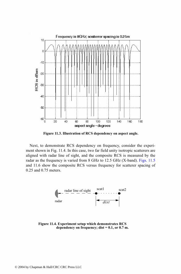
© 200
Next, to demonstrate RCS dependency on frequency, consider the experi-ment shown in Fig. 11.4. In this case, two far field unity isotropic scatterers arealigned with radar line of sight, and the composite RCS is measured by theradar as the frequency is varied from 8 GHz to 12.5 GHz (X-band). Figs. 11.5and 11.6 show the composite RCS versus frequency for scatterer spacing of0.25 and 0.75 meters.
Figure 11.3. Illustration of RCS dependency on aspect angle.
radar
radar line of sight
dist
scat1 scat2
Figure 11.4. Experiment setup which demonstrates RCS dependency on frequency; dist = 0.1, or 0.7 m.
4 by Chapman & Hall/CRC CRC Press LLC
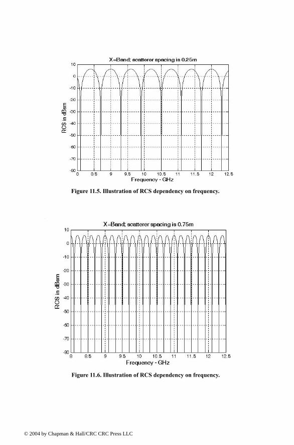
© 200
Figure 11.5. Illustration of RCS dependency on frequency.
Figure 11.6. Illustration of RCS dependency on frequency.
4 by Chapman & Hall/CRC CRC Press LLC
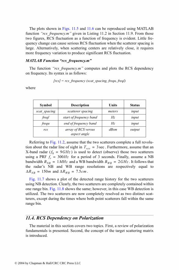
© 200
The plots shown in Figs. 11.5 and 11.6 can be reproduced using MATLABfunction rcs_frequency.m given in Listing 11.2 in Section 11.9. From thosetwo figures, RCS fluctuation as a function of frequency is evident. Little fre-quency change can cause serious RCS fluctuation when the scatterer spacing islarge. Alternatively, when scattering centers are relatively close, it requiresmore frequency variation to produce significant RCS fluctuation.
MATLAB Function rcs_frequency.m
The function rcs_frequency.m computes and plots the RCS dependencyon frequency. Its syntax is as follows:
[rcs] = rcs_frequency (scat_spacing, frequ, freql)
where
Referring to Fig. 11.2, assume that the two scatterers complete a full revolu-tion about the radar line of sight in . Furthermore, assume that anX-band radar ( ) is used to detect (observe) those two scatterersusing a PRF for a period of 3 seconds. Finally, assume a NBbandwidth and a WB bandwidth . It follows thatthe radars NB and WB range resolutions are respectively equal to
and .
Fig. 11.7 shows a plot of the detected range history for the two scatterersusing NB detection. Clearly, the two scatterers are completely contained withinone range bin. Fig. 11.8 shows the same; however, in this case WB detection isutilized. The two scatterers are now completely resolved as two distinct scat-terers, except during the times where both point scatterers fall within the samerange bin.
11.4. RCS Dependency on PolarizationThe material in this section covers two topics. First, a review of polarization
fundamentals is presented. Second, the concept of the target scattering matrixis introduced.
Symbol Description Units Status
scat_spacing scatterer spacing meters input
freql start of frequency band Hz input
frequ end of frequency band Hz input
rcs array of RCS versus aspect angle
dBsm output
Trev 3sec=f0 9GHz=
fr 300Hz=BNB 1MHz= BWB 2GHz=
∆RNB 150m= ∆RWB 7.5cm=
4 by Chapman & Hall/CRC CRC Press LLC
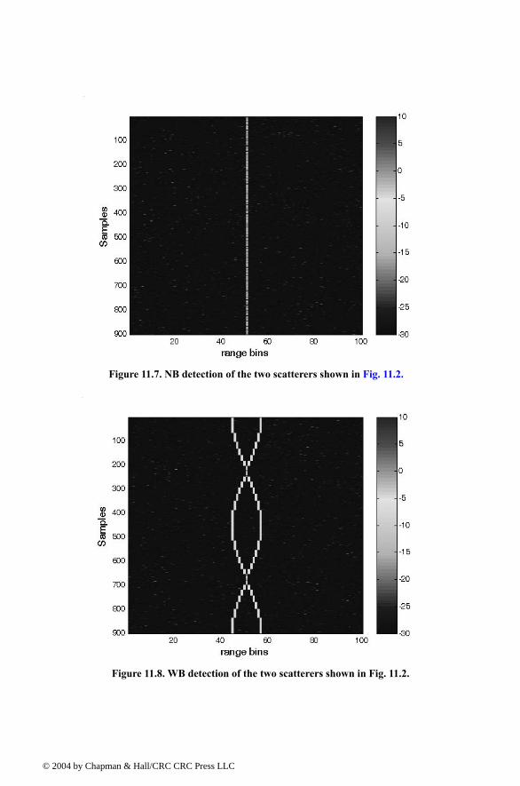
© 200
Figure 11.7. NB detection of the two scatterers shown in Fig. 11.2.
Figure 11.8. WB detection of the two scatterers shown in Fig. 11.2.
4 by Chapman & Hall/CRC CRC Press LLC
© 200
11.4.1. Polarization
The x and y electric field components for a wave traveling along the positivez direction are given by
(11.7)
(11.8)
where , is the wave frequency, the angle is the time phaseangle which leads , and, finally, and are, respectively, the waveamplitudes along the x and y directions. When two or more electromagneticwaves combine, their electric fields are integrated vectorially at each point inspace for any specified time. In general, the combined vector traces an ellipsewhen observed in the x-y plane. This is illustrated in Fig. 11.9.
The ratio of the major to the minor axes of the polarization ellipse is calledthe Axial Ratio (AR). When AR is unity, the polarization ellipse becomes a cir-cle, and the resultant wave is then called circularly polarized. Alternatively,when and the wave becomes linearly polarized.
Eqs. (11.7) and (11.8) can be combined to give the instantaneous total elec-tric field,
(11.9)
Ex E1 ωt kz( )sin=
Ey E2 ωt kz δ+( )sin=
k 2π λ⁄= ω δEy Ex E1 E2
E1 0= AR ∞=
E a xE1 ωt kz( )sin a yE2 ωt kz δ+( )sin+=
Figure 11.9. Electric field components along the x and y directions. The positive z direction is out of the page.
X
Y
Z E1
E2
E
4 by Chapman & Hall/CRC CRC Press LLC
© 200
where and are unit vectors along the x and y directions, respectively. At, and , then by replacing
by the ratio and by using trigonometry properties Eq. (11.9)can be rewritten as
(11.10)
Note that Eq. (11.10) has no dependency on .
In the most general case, the polarization ellipse may have any orientation,as illustrated in Fig. 11.10. The angle is called the tilt angle of the ellipse. Inthis case, AR is given by
(11.11)
When , the wave is said to be linearly polarized in the y direction,while if the wave is said to be linearly polarized in the x direction.Polarization can also be linear at an angle of when and
. When and , the wave is said to be Left Circu-larly Polarized (LCP), while if the wave is said to Right CircularlyPolarized (RCP). It is a common notation to call the linear polarizations alongthe x and y directions by the names horizontal and vertical polarizations,respectively.
a x a yz 0= Ex E1 ωt( )sin= Ey E2 ωt δ+( )sin=
ωt( )sin Ex E1⁄
Ex2
E12
-----2ExEy δcos
E1E2---------------------------
Ey2
E22
-----+ δsin( )2=
ωt
ξ
AR OAOB--------= 1 AR ∞≤ ≤( )
E1 0=E2 0=
45° E1 E2=ξ 45°= E1 E2= δ 90°=
δ 90°=
Figure 11.10. Polarization ellipse in the general case.
X
Y
Z E1
E2
E
O
A
B
Ex
Ey
ξ
4 by Chapman & Hall/CRC CRC Press LLC
© 200
In general, an arbitrarily polarized electric field may be written as the sum oftwo circularly polarized fields. More precisely,
(11.12)
where and are the RCP and LCP fields, respectively. Similarly, theRCP and LCP waves can be written as
(11.13)
(11.14)
where and are the fields with vertical and horizontal polarizations,respectively. Combining Eqs. (11.13) and (11.14) yields
(11.15)
(11.16)
Using matrix notation Eqs. (11.15) and (11.16) can be rewritten as
(11.17)
(11.18)
For many targets the scattered waves will have different polarization than theincident waves. This phenomenon is known as depolarization or cross-polar-ization. However, perfect reflectors reflect waves in such a fashion that an inci-dent wave with horizontal polarization remains horizontal, and an incidentwave with vertical polarization remains vertical but is phase shifted .Additionally, an incident wave which is RCP becomes LCP when reflected,and a wave which is LCP becomes RCP after reflection from a perfect reflec-tor. Therefore, when a radar uses LCP waves for transmission, the receivingantenna needs to be RCP polarized in order to capture the PP RCS, and LCR tomeasure the OP RCS.
E ER EL+=
ER EL
ER EV jEH+=
EL EV j EH=
EV EH
EREH jEV
2---------------------=
ELEH jEV+
2---------------------=
ER
EL
12
------- 1 j
1 jEH
EV
T[ ]EH
EV
= =
EH
EV
12
------- 1 1j j
ER
EL
T[ ] 1 EH
EV
= =
180°
4 by Chapman & Hall/CRC CRC Press LLC
© 200
Example:
Plot the locus of the electric field vector for the following cases:
case1:
case 2:
case 3:
case 4:
Solution:
The MATLAB program example11_1.m was developed to calculate andplot the loci of the electric fields. Figs. 11.11 through 11.14 show the desiredelectric fields loci. See listing 11.3 in Section 11.9.
E t z,( ) a x ω0t 2πzλ
---------+ cos a y 3 ω0t 2πz
λ---------+
cos+=
E t z,( ) a x ω0t 2πzλ
---------+ cos a y ω0t 2πz
λ---------+
sin+=
E t z,( ) a x ω0t 2πzλ
---------+ cos a y ω0t 2πz
λ--------- π
6---+ +
cos+=
E t z,( ) a x ω0t 2πzλ
---------+ cos a y 3 ω0t 2πz
λ--------- π
3---+ +
cos+=
Figure 11.11. Linearly polarized electric field.
4 by Chapman & Hall/CRC CRC Press LLC
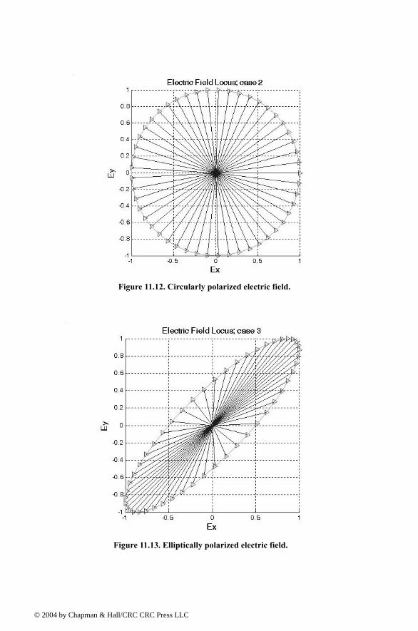
© 200
Figure 11.12. Circularly polarized electric field.
Figure 11.13. Elliptically polarized electric field.
4 by Chapman & Hall/CRC CRC Press LLC
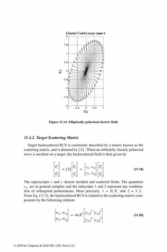
© 200
11.4.2. Target Scattering Matrix
Target backscattered RCS is commonly described by a matrix known as thescattering matrix, and is denoted by . When an arbitrarily linearly polarizedwave is incident on a target, the backscattered field is then given by
(11.19)
The superscripts and denote incident and scattered fields. The quantities are in general complex and the subscripts 1 and 2 represent any combina-
tion of orthogonal polarizations. More precisely, , and .From Eq. (11.3), the backscattered RCS is related to the scattering matrix com-ponents by the following relation:
(11.20)
Figure 11.14. Elliptically polarized electric field.
S[ ]
E1s
E2s
S[ ]E1
i
E2i
s11 s12
s21 s22
E1i
E2i
= =
i ssij
1 H R,= 2 V L,=
σ11 σ12
σ21 σ22
4πR2 s112 s12
2
s212 s22
2=
4 by Chapman & Hall/CRC CRC Press LLC
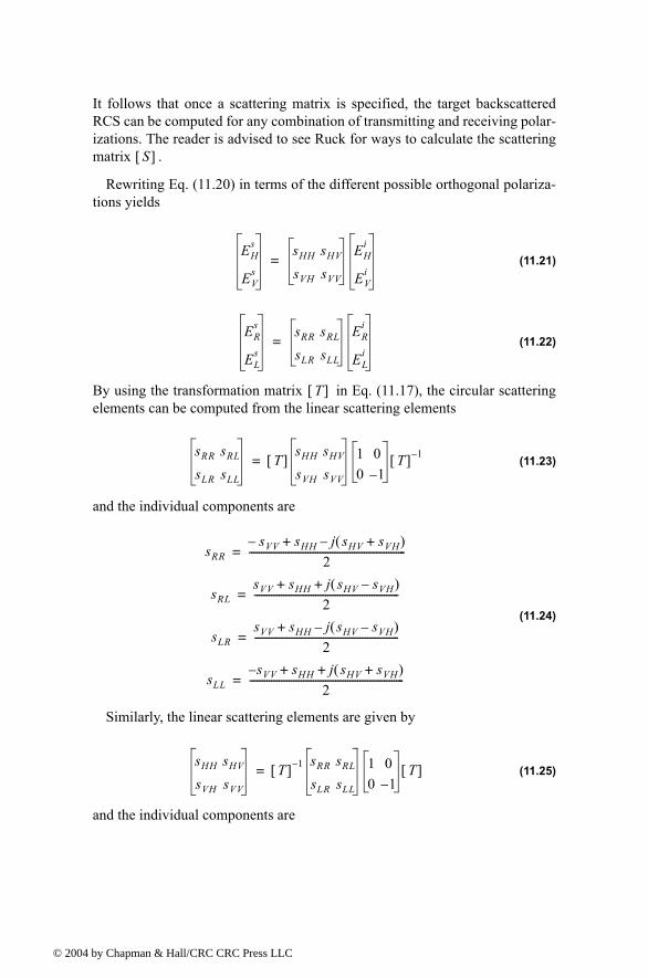
© 200
It follows that once a scattering matrix is specified, the target backscatteredRCS can be computed for any combination of transmitting and receiving polar-izations. The reader is advised to see Ruck for ways to calculate the scatteringmatrix .
Rewriting Eq. (11.20) in terms of the different possible orthogonal polariza-tions yields
(11.21)
(11.22)
By using the transformation matrix in Eq. (11.17), the circular scatteringelements can be computed from the linear scattering elements
(11.23)
and the individual components are
(11.24)
Similarly, the linear scattering elements are given by
(11.25)
and the individual components are
S[ ]
EHs
EVs
sHH sHV
sVH sVV
EHi
EVi
=
ERs
ELs
sRR sRL
sLR sLL
ERi
ELi
=
T[ ]
sRR sRL
sLR sLL
T[ ]sHH sHV
sVH sVV
1 00 1
T[ ] 1=
sRRsVV sHH j sHV sVH+( )+
2----------------------------------------------------------------=
sRLsVV sHH j sHV sVH( )+ +
2-----------------------------------------------------------=
sLRsVV sHH j sHV sVH( )+
2-----------------------------------------------------------=
sLLs VV sHH j sHV sVH+( )+ +
2---------------------------------------------------------------=
sHH sHV
sVH sVV
T[ ] 1 sRR sRL
sLR sLL
1 00 1
T[ ]=
4 by Chapman & Hall/CRC CRC Press LLC
© 200
(11.26)
11.5. RCS of Simple Objects This section presents examples of backscattered radar cross section for a
number of simple shape objects. In all cases, except for the perfectly conduct-ing sphere, only optical region approximations are presented. Radar designersand RCS engineers consider the perfectly conducting sphere to be the simplesttarget to examine. Even in this case, the complexity of the exact solution, whencompared to the optical region approximation, is overwhelming. Most formu-las presented are Physical Optics (PO) approximation for the backscatteredRCS measured by a far field radar in the direction ( ), as illustrated in Fig.11.15.
In this section, it is assumed that the radar is always illuminating an objectfrom the positive z-direction.
sHHsRR sRL sLR sLL+ +
2------------------------------------------------------=
sVHj sRR sLR sRL sLL+( )
2--------------------------------------------------------=
sHVj sRR sLR sRL sLL+( )
2-----------------------------------------------------------=
sVVsRR sLL jsRL sLR++ +
2----------------------------------------------------=
θ ϕ,
θ
ϕ
Z
Y
X
Direction toreceiving radar
Figure 11.15. Direction of antenna receiving backscattered waves.
sphere
4 by Chapman & Hall/CRC CRC Press LLC
© 200
11.5.1. Sphere
Due to symmetry, waves scattered from a perfectly conducting sphere areco-polarized (have the same polarization) with the incident waves. This meansthat the cross-polarized backscattered waves are practically zero. For example,if the incident waves were Left Circularly Polarized (LCP), then the backscat-tered waves will also be LCP. However, because of the opposite direction ofpropagation of the backscattered waves, they are considered to be Right Circu-larly Polarized (RCP) by the receiving antenna. Therefore, the PP backscat-tered waves from a sphere are LCP, while the OP backscattered waves arenegligible.
The normalized exact backscattered RCS for a perfectly conducting sphereis a Mie series given by
(11.27)
where is the radius of the sphere, , is the wavelength, is thespherical Bessel of the first kind of order n, and is the Hankel function oforder n, and is given by
(11.28)
is the spherical Bessel function of the second kind of order n. Plots of thenormalized perfectly conducting sphere RCS as a function of its circumferencein wavelength units are shown in Figs. 11.16a and 11.16b. These plots can bereproduced using the function rcs_sphere.m given in Listing 11.4 in Section11.9.
In Fig. 11.16, three regions are identified. First is the optical region (corre-sponds to a large sphere). In this case,
(11.29)
Second is the Rayleigh region (small sphere). In this case,
(11.30)
The region between the optical and Rayleigh regions is oscillatory in natureand is called the Mie or resonance region.
σ
πr2-------- j
kr----- 1( )n 2n 1+( )
krJn 1 kr( ) nJn kr( )
krHn 11( ) kr( ) nHn
1( ) kr( )-----------------------------------------------------------
Jn kr( )
Hn1( ) kr( )
--------------------
n 1=
∞
∑=
r k 2π λ⁄= λ JnHn
1( )
Hn1( ) kr( ) Jn kr( ) jYn kr( )+=
Yn
σ πr2= r λ»
σ 9πr2 kr( )4≈ r λ«
4 by Chapman & Hall/CRC CRC Press LLC
© 200
1 2 3 4 5 6 7 8 9 1 0 1 1 12 13 14 1 50
0 .2
0 .4
0 .6
0 .8
1
1 .2
1 .4
1 .6
1 .8
2
Figure 11.16a. Normalized backscattered RCS for a perfectly conducting sphere.
2πr λ⁄
σ
πr2--------
10-2
10-1
100
101
102
-25
-20
-15
-10
-5
0
5
S phere c irc um ferenc e in wavelengths
No
rma
lize
d s
ph
ere
RC
S -
dB
Figure 11.16b. Normalized backscattered RCS for a perfectly conducting sphere using semi-log scale.
optical region
Mie region
Rayleighregion
4 by Chapman & Hall/CRC CRC Press LLC
© 200
The backscattered RCS for a perfectly conducting sphere is constant in theoptical region. For this reason, radar designers typically use spheres of knowncross sections to experimentally calibrate radar systems. For this purpose,spheres are flown attached to balloons. In order to obtain Doppler shift,spheres of known RCS are dropped out of an airplane and towed behind theairplane whose velocity is known to the radar.
11.5.2. Ellipsoid
An ellipsoid centered at (0,0,0) is shown in Fig. 11.17. It is defined by thefollowing equation:
(11.31)
One widely accepted approximation for the ellipsoid backscattered RCS isgiven by
(11.32)
When , the ellipsoid becomes roll symmetric. Thus, the RCS is inde-pendent of , and Eq. (11.32) is reduced to
xa---
2 yb---
2 zc--
2+ + 1=
σ πa2b2c2
a2 θsin( )2 ϕcos( )2 b2 θsin( )2 ϕsin( )2 c2 θcos( )2+ +( )2
-----------------------------------------------------------------------------------------------------------------------------------=
a b=ϕ
θ
ϕ
Z
Y
X
Direction toreceiving radar
Figure 11.17. Ellipsoid.
a
c
b
4 by Chapman & Hall/CRC CRC Press LLC
© 200
(11.33)
and for the case when ,
(11.34)
Note that Eq. (11.34) defines the backscattered RCS of a sphere. This shouldbe expected, since under the condition the ellipsoid becomes asphere. Fig. 11.18a shows the backscattered RCS for an ellipsoid versus for
. This plot can be generated using MATLAB program fig11_18a.mgiven in Listing 11.5 in Section 11.9. Note that at normal incidence ( )the RCS corresponds to that of a sphere of radius , and is often referred to asthe broadside specular RCS value.
MATLAB Function rcs_ellipsoid.m
The function rcs_ellipsoid.m computes and plots the RCS of an ellipsoidversus aspect angle. It is given in Listing 11.6 in Section 11.9, and its syntax isas follows:
[rcs] = rcs_ellipsoid (a, b, c, phi)
σ πb4c2
a2 θsin( )2 c2 θcos( )2+( )2
--------------------------------------------------------------=
a b c= =
σ πc2=
a b c= =θ
ϕ 45°=θ 90°=
c
Figure 11.18a. Ellipsoid backscattered RCS versus aspect angle.
4 by Chapman & Hall/CRC CRC Press LLC
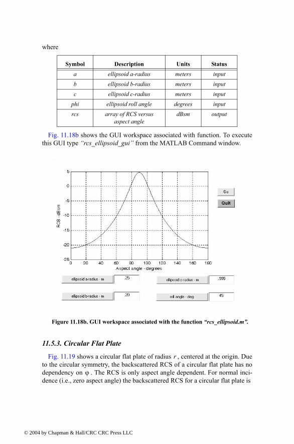
© 200
where
Fig. 11.18b shows the GUI workspace associated with function. To executethis GUI type rcs_ellipsoid_gui from the MATLAB Command window.
11.5.3. Circular Flat Plate
Fig. 11.19 shows a circular flat plate of radius , centered at the origin. Dueto the circular symmetry, the backscattered RCS of a circular flat plate has nodependency on . The RCS is only aspect angle dependent. For normal inci-dence (i.e., zero aspect angle) the backscattered RCS for a circular flat plate is
Symbol Description Units Status
a ellipsoid a-radius meters input
b ellipsoid b-radius meters input
c ellipsoid c-radius meters input
phi ellipsoid roll angle degrees input
rcs array of RCS versus aspect angle
dBsm output
Figure 11.18b. GUI workspace associated with the function rcs_ellipsoid.m.
r
ϕ
4 by Chapman & Hall/CRC CRC Press LLC
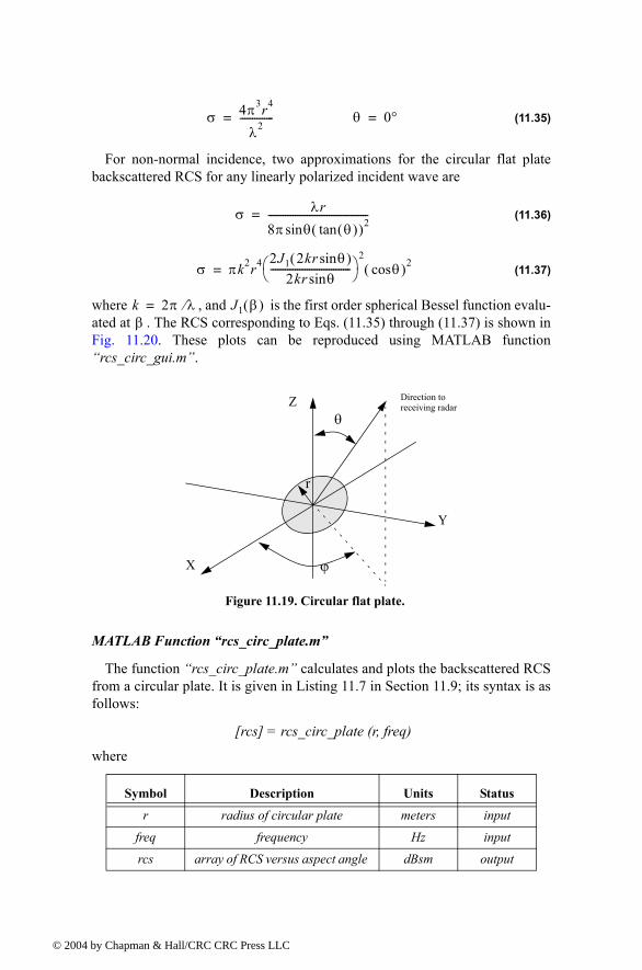
© 200
(11.35)
For non-normal incidence, two approximations for the circular flat platebackscattered RCS for any linearly polarized incident wave are
(11.36)
(11.37)
where , and is the first order spherical Bessel function evalu-ated at . The RCS corresponding to Eqs. (11.35) through (11.37) is shown inFig. 11.20. These plots can be reproduced using MATLAB functionrcs_circ_gui.m.
MATLAB Function rcs_circ_plate.m
The function rcs_circ_plate.m calculates and plots the backscattered RCSfrom a circular plate. It is given in Listing 11.7 in Section 11.9; its syntax is asfollows:
[rcs] = rcs_circ_plate (r, freq)
where
Symbol Description Units Status
r radius of circular plate meters input
freq frequency Hz input
rcs array of RCS versus aspect angle dBsm output
σ 4π3r4
λ2--------------= θ 0°=
σ λr8π θsin θ( )tan( )2-----------------------------------------=
σ πk2r4 2J1 2kr θsin( )2kr θsin
---------------------------------
2θcos( )2=
k 2π λ⁄= J1 β( )β
θ
ϕ
Z
Y
X
Direction toreceiving radar
Figure 11.19. Circular flat plate.
r
4 by Chapman & Hall/CRC CRC Press LLC
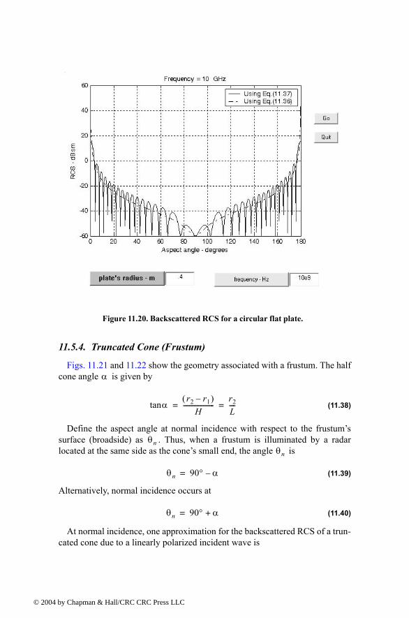
© 200
11.5.4. Truncated Cone (Frustum)
Figs. 11.21 and 11.22 show the geometry associated with a frustum. The halfcone angle is given by
(11.38)
Define the aspect angle at normal incidence with respect to the frustumssurface (broadside) as . Thus, when a frustum is illuminated by a radarlocated at the same side as the cones small end, the angle is
(11.39)
Alternatively, normal incidence occurs at
(11.40)
At normal incidence, one approximation for the backscattered RCS of a trun-cated cone due to a linearly polarized incident wave is
Figure 11.20. Backscattered RCS for a circular flat plate.
α
αtanr2 r1( )
H--------------------
r2
L----= =
θnθn
θn 90° α=
θn 90° α+=
4 by Chapman & Hall/CRC CRC Press LLC
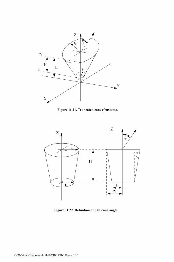
© 200
Figure 11.21. Truncated cone (frustum).
Z
Y
X
r2
Lz1
z2
r1
θ
H
r2
r1
H
Figure 11.22. Definition of half cone angle.
ZZ
α
θ
r1
r2
4 by Chapman & Hall/CRC CRC Press LLC
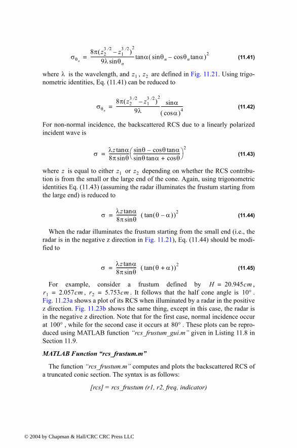
© 200
(11.41)
where is the wavelength, and , are defined in Fig. 11.21. Using trigo-nometric identities, Eq. (11.41) can be reduced to
(11.42)
For non-normal incidence, the backscattered RCS due to a linearly polarizedincident wave is
(11.43)
where is equal to either or depending on whether the RCS contribu-tion is from the small or the large end of the cone. Again, using trigonometricidentities Eq. (11.43) (assuming the radar illuminates the frustum starting fromthe large end) is reduced to
(11.44)
When the radar illuminates the frustum starting from the small end (i.e., theradar is in the negative z direction in Fig. 11.21), Eq. (11.44) should be modi-fied to
(11.45)
For example, consider a frustum defined by ,, . It follows that the half cone angle is .
Fig. 11.23a shows a plot of its RCS when illuminated by a radar in the positivez direction. Fig. 11.23b shows the same thing, except in this case, the radar isin the negative z direction. Note that for the first case, normal incidence occurat , while for the second case it occurs at . These plots can be repro-duced using MATLAB function rcs_frustum_gui.m given in Listing 11.8 inSection 11.9.
MATLAB Function rcs_frustum.m
The function rcs_frustum.m computes and plots the backscattered RCS ofa truncated conic section. The syntax is as follows:
[rcs] = rcs_frustum (r1, r2, freq, indicator)
σθn
8π z23 2⁄ z1
3 2⁄( )2
9λ θnsin--------------------------------------- α θnsin θncos αtan( )2tan=
λ z1 z2
σθn
8π z23 2⁄ z1
3 2⁄( )2
9λ--------------------------------------- αsin
αcos( )4-------------------=
σ λz αtan8π θsin------------------ θsin θ αtancos
θ αtansin θcos+------------------------------------------
2=
z z1 z2
σ λz αtan8π θsin------------------ θ α( )tan( )2=
σ λz αtan8π θsin------------------ θ α+( )tan( )2=
H 20.945cm=r1 2.057cm= r2 5.753cm= 10°
100° 80°
4 by Chapman & Hall/CRC CRC Press LLC
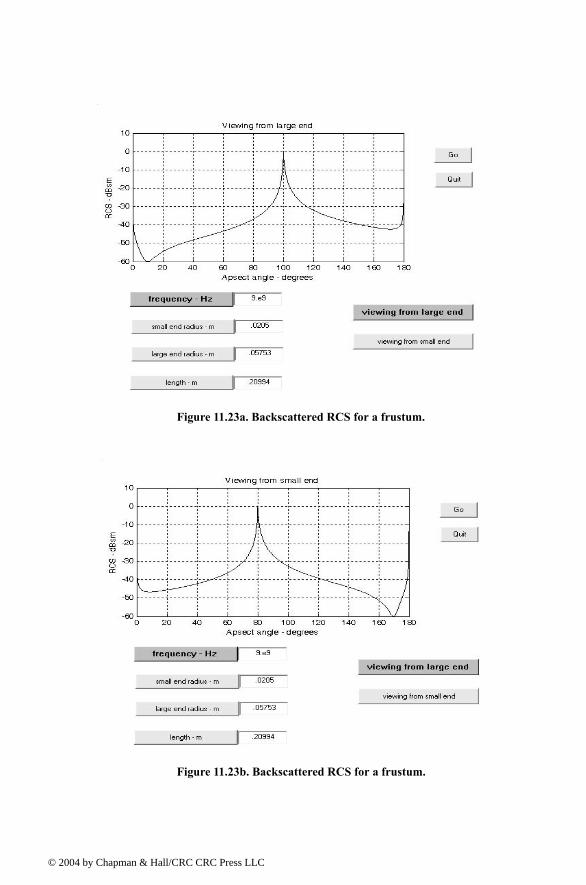
© 200
Figure 11.23a. Backscattered RCS for a frustum.
Figure 11.23b. Backscattered RCS for a frustum.
4 by Chapman & Hall/CRC CRC Press LLC
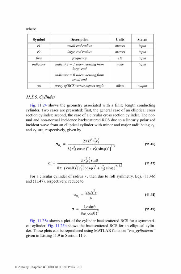
© 200
where
11.5.5. Cylinder
Fig. 11.24 shows the geometry associated with a finite length conductingcylinder. Two cases are presented: first, the general case of an elliptical crosssection cylinder; second, the case of a circular cross section cylinder. The nor-mal and non-normal incidence backscattered RCS due to a linearly polarizedincident wave from an elliptical cylinder with minor and major radii being and are, respectively, given by
(11.46)
(11.47)
For a circular cylinder of radius , then due to roll symmetry, Eqs. (11.46)and (11.47), respectively, reduce to
(11.48)
(11.49)
Fig. 11.25a shows a plot of the cylinder backscattered RCS for a symmetri-cal cylinder. Fig. 11.25b shows the backscattered RCS for an elliptical cylin-der. These plots can be reproduced using MATLAB function rcs_cylinder.mgiven in Listing 11.9 in Section 11.9.
Symbol Description Units Status
r1 small end radius meters input
r2 large end radius meters input
freq frequency Hz input
indicator indicator = 1 when viewing from large end
indicator = 0 when viewing from small end
none input
rcs array of RCS versus aspect angle dBsm output
r1r2
σθn
2πH2r22r1
2
λ r12 ϕcos( )2 r2
2 ϕsin( )2+[ ]1.5
--------------------------------------------------------------------=
σλr2
2r12 θsin
8π θcos( )2 r12 ϕcos( )2 r2
2 ϕsin( )2+[ ]1.5
-----------------------------------------------------------------------------------------------=
r
σθn
2πH2rλ
----------------=
σ λr θsin8π θcos( )2--------------------------=
4 by Chapman & Hall/CRC CRC Press LLC
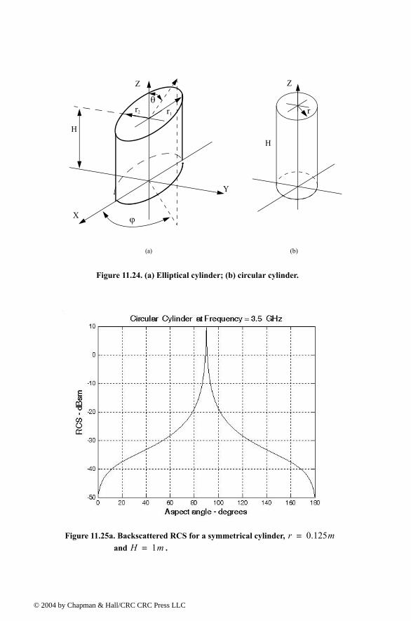
© 200
Z
Y
X
r1r2
θ
H
ϕ
Z
r
H
(a) (b)
Figure 11.24. (a) Elliptical cylinder; (b) circular cylinder.
Figure 11.25a. Backscattered RCS for a symmetrical cylinder, and .
r 0.125m=H 1m=
4 by Chapman & Hall/CRC CRC Press LLC
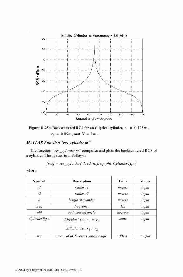
© 200
MATLAB Function rcs_cylinder.m
The function rcs_cylinder.m computes and plots the backscattered RCS ofa cylinder. The syntax is as follows:
[rcs] = rcs_cylinder(r1, r2, h, freq, phi, CylinderType)
where
Symbol Description Units Status
r1 radius r1 meters input
r2 radius r2 meters input
h length of cylinder meters input
freq frequency Hz input
phi roll viewing angle degrees input
CylinderType Circular, i.e.,
Elliptic, i.e.,
none input
rcs array of RCS versus aspect angle dBsm output
Figure 11.25b. Backscattered RCS for an elliptical cylinder, ,
, and .
r1 0.125m=
r2 0.05m= H 1m=
r1 r2=
r1 r2≠
4 by Chapman & Hall/CRC CRC Press LLC
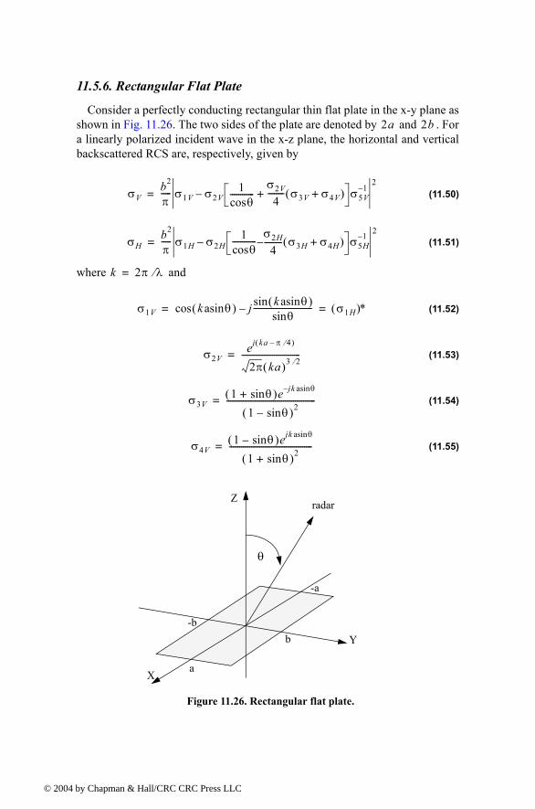
© 200
11.5.6. Rectangular Flat Plate
Consider a perfectly conducting rectangular thin flat plate in the x-y plane asshown in Fig. 11.26. The two sides of the plate are denoted by and . Fora linearly polarized incident wave in the x-z plane, the horizontal and verticalbackscattered RCS are, respectively, given by
(11.50)
(11.51)
where and
(11.52)
(11.53)
(11.54)
(11.55)
2a 2b
σVb2
π----- σ1V σ2V
1θcos
------------σ2V
4-------- σ3V σ4V+( )+ σ5V
12
=
σHb2
π----- σ1H σ2H
1θcos
------------ σ2H
4--------- σ3H σ4H+( ) σ5H
12
=
k 2π λ⁄=
σ1V k θasin( )cos j k θasin( )sinθsin
----------------------------- σ1H( )∗= =
σ2Vej ka π 4⁄( )
2π ka( )3 2⁄-----------------------------=
σ3V1 θsin+( )e jk θasin
1 θsin( )2--------------------------------------------=
σ4V1 θsin( )ejk θasin
1 θsin+( )2-----------------------------------------=
Figure 11.26. Rectangular flat plate.
Z
Y
X
θ
b-b
-a
a
radar
4 by Chapman & Hall/CRC CRC Press LLC
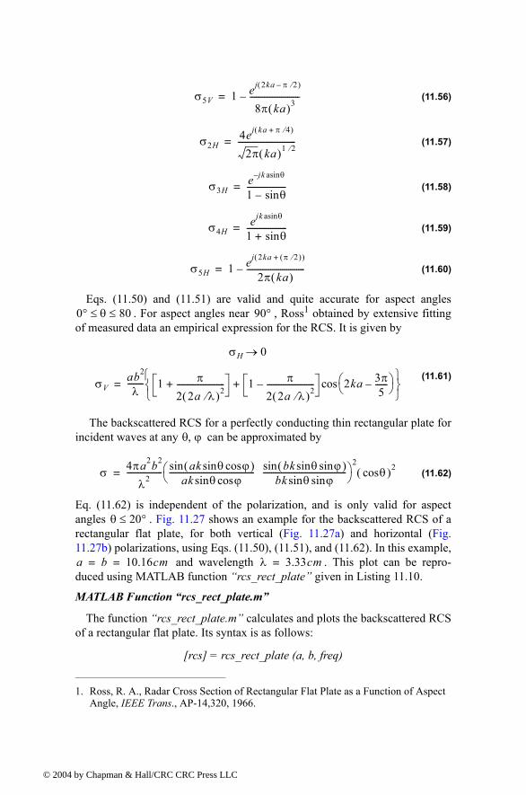
© 200
(11.56)
(11.57)
(11.58)
(11.59)
(11.60)
Eqs. (11.50) and (11.51) are valid and quite accurate for aspect angles. For aspect angles near , Ross1 obtained by extensive fitting
of measured data an empirical expression for the RCS. It is given by
(11.61)
The backscattered RCS for a perfectly conducting thin rectangular plate forincident waves at any can be approximated by
(11.62)
Eq. (11.62) is independent of the polarization, and is only valid for aspectangles . Fig. 11.27 shows an example for the backscattered RCS of arectangular flat plate, for both vertical (Fig. 11.27a) and horizontal (Fig.11.27b) polarizations, using Eqs. (11.50), (11.51), and (11.62). In this example,
and wavelength . This plot can be repro-duced using MATLAB function rcs_rect_plate given in Listing 11.10.
MATLAB Function rcs_rect_plate.m
The function rcs_rect_plate.m calculates and plots the backscattered RCSof a rectangular flat plate. Its syntax is as follows:
[rcs] = rcs_rect_plate (a, b, freq)
1. Ross, R. A., Radar Cross Section of Rectangular Flat Plate as a Function of Aspect Angle, IEEE Trans., AP-14,320, 1966.
σ5V 1 ej 2ka π 2⁄( )
8π ka( )3-------------------------=
σ2H4ej ka π 4⁄+( )
2π ka( )1 2⁄-----------------------------=
σ3He jk θasin
1 θsin--------------------=
σ4Hejk θasin
1 θsin+--------------------=
σ5H 1 ej 2ka π 2⁄( )+( )
2π ka( )-----------------------------=
0° θ 80≤ ≤ 90°
σH 0→
σVab2
λ-------- 1 π
2 2a λ⁄( )2------------------------+ 1 π
2 2a λ⁄( )2------------------------ 2ka 3π
5------
cos+
=
θ ϕ,
σ 4πa2b2
λ2------------------ ak θsin ϕcos( )sin
ak θsin ϕcos------------------------------------------- bk θsin ϕsin( )sin
bk θsin ϕsin------------------------------------------
2
θcos( )2=
θ 20°≤
a b 10.16cm= = λ 3.33cm=
4 by Chapman & Hall/CRC CRC Press LLC
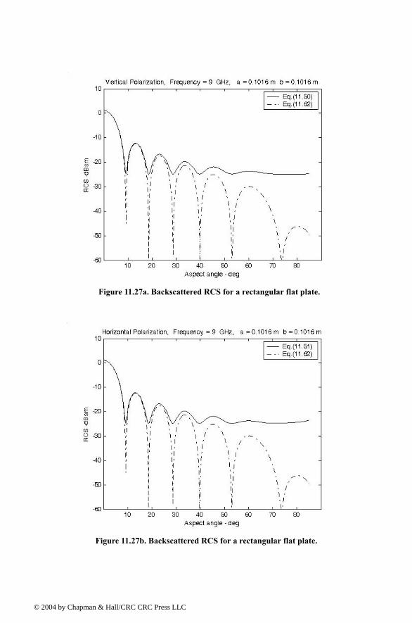
© 200
Figure 11.27a. Backscattered RCS for a rectangular flat plate.
Figure 11.27b. Backscattered RCS for a rectangular flat plate.
4 by Chapman & Hall/CRC CRC Press LLC
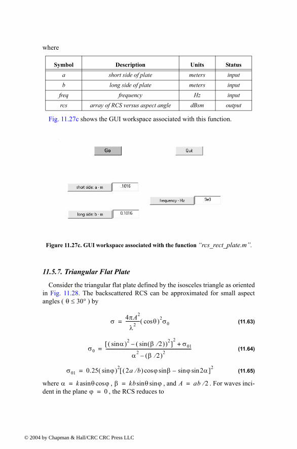
© 200
where
Fig. 11.27c shows the GUI workspace associated with this function.
11.5.7. Triangular Flat Plate
Consider the triangular flat plate defined by the isosceles triangle as orientedin Fig. 11.28. The backscattered RCS can be approximated for small aspectangles ( ) by
(11.63)
(11.64)
(11.65)
where , , and . For waves inci-dent in the plane , the RCS reduces to
Symbol Description Units Status
a short side of plate meters input
b long side of plate meters input
freq frequency Hz input
rcs array of RCS versus aspect angle dBsm output
Figure 11.27c. GUI workspace associated with the function rcs_rect_plate.m.
θ 30°≤
σ 4πA2
λ2------------- θcos( )2σ0=
σ0αsin( )2 β 2⁄( )sin( )2[ ]
2σ01+
α2 β 2⁄( )2----------------------------------------------------------------------------=
σ01 0.25 ϕsin( )2 2a b⁄( ) ϕ βsincos ϕ 2αsinsin[ ]2=
α k θ ϕcosasin= β kb θ ϕsinsin= A ab 2⁄=ϕ 0=
4 by Chapman & Hall/CRC CRC Press LLC
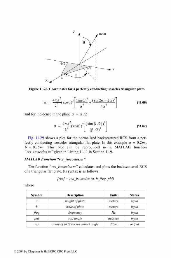
© 200
(11.66)
and for incidence in the plane
(11.67)
Fig. 11.29 shows a plot for the normalized backscattered RCS from a per-fectly conducting isosceles triangular flat plate. In this example ,
. This plot can be reproduced using MATLAB functionrcs_isosceles.m given in Listing 11.11 in Section 11.9.
MATLAB Function rcs_isosceles.m
The function rcs_isosceles.m calculates and plots the backscattered RCSof a triangular flat plate. Its syntax is as follows:
[rcs] = rcs_isosceles (a, b, freq, phi)
where
Symbol Description Units Status
a height of plate meters input
b base of plate meters input
freq frequency Hz input
phi roll angle degrees input
rcs array of RCS versus aspect angle dBsm output
Figure 11.28. Coordinates for a perfectly conducting isosceles triangular plate.
Z
Y
X
θ
b/2-b/2
a
radar
ϕ
σ 4πA2
λ2------------- θcos( )2 αsin( )4
α4------------------ 2αsin 2α( )2
4α4-----------------------------------+=
ϕ π 2⁄=
σ 4πA2
λ2------------- θcos( )2 β 2⁄( )sin( )4
β 2⁄( )4------------------------------=
a 0.2m=b 0.75m=
4 by Chapman & Hall/CRC CRC Press LLC
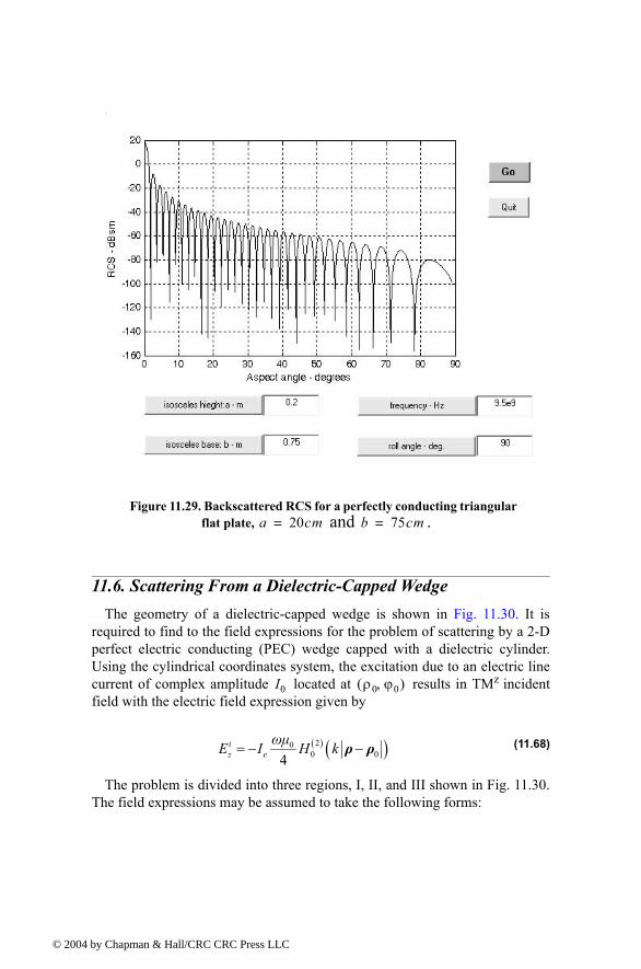
© 200
11.6. Scattering From a Dielectric-Capped WedgeThe geometry of a dielectric-capped wedge is shown in Fig. 11.30. It is
required to find to the field expressions for the problem of scattering by a 2-Dperfect electric conducting (PEC) wedge capped with a dielectric cylinder.Using the cylindrical coordinates system, the excitation due to an electric linecurrent of complex amplitude located at results in TMz incidentfield with the electric field expression given by
(11.68)
The problem is divided into three regions, I, II, and III shown in Fig. 11.30.The field expressions may be assumed to take the following forms:
Figure 11.29. Backscattered RCS for a perfectly conducting triangular flat plate, and .a 20cm= b 75cm=
I0 ρ0 ϕ0,( )
( ) ( )200 04
iz e
ωµE I H k= − −ρ ρ
4 by Chapman & Hall/CRC CRC Press LLC
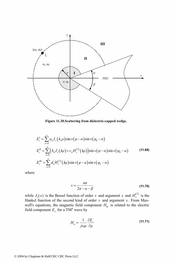
© 200
(11.69)
where
(11.70)
while is the Bessel function of order and argument and is theHankel function of the second kind of order and argument . From Max-well's equations, the magnetic field component is related to the electricfield component for a TMz wave by
(11.71)
x
y
α
β
I
II
III (ρ0, ϕ0)
PEC ε, µ0
ε0, µ0
Ie
a
Figure 11.30.Scattering from dielectric-capped wedge.
( ) ( ) ( )
( ) ( ) ( )( ) ( ) ( )
( ) ( ) ( ) ( )
I1 0
0
2II0
0
2III0
0
sin sin
sin sin
sin sin
z n vn
z n v n νn
z n νn
E a J k ρ v φ α v φ α
E b J kρ c H kρ v φ α v φ α
E d H kρ v φ α v φ α
∞
=
∞
=
∞
=
= − −
= + − −
= − −
∑
∑
∑
2nπv
π α β=
− −
Jv x( ) v x Hv2( )
v xHϕ
Ez
1 zφ
EHjωµ ρ
∂=
∂
4 by Chapman & Hall/CRC CRC Press LLC
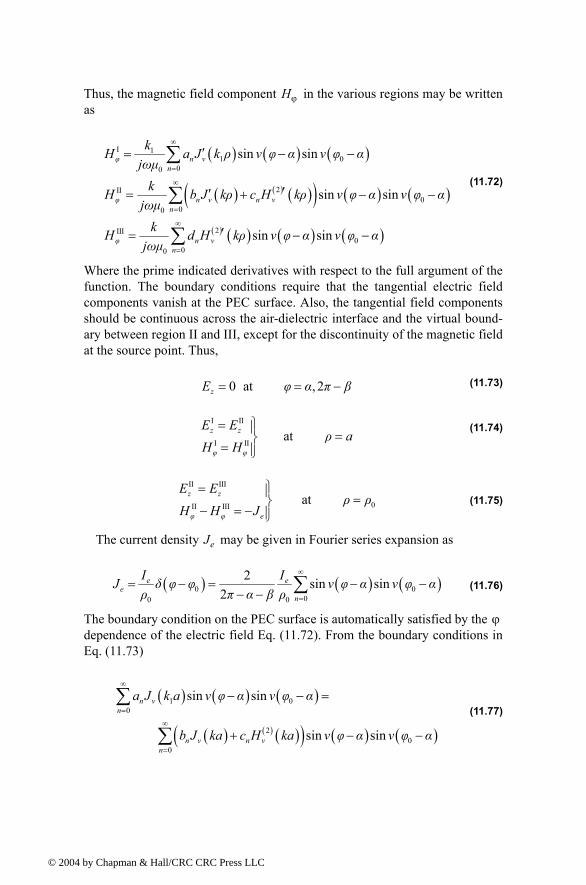
© 200
Thus, the magnetic field component in the various regions may be writtenas
(11.72)
Where the prime indicated derivatives with respect to the full argument of thefunction. The boundary conditions require that the tangential electric fieldcomponents vanish at the PEC surface. Also, the tangential field componentsshould be continuous across the air-dielectric interface and the virtual bound-ary between region II and III, except for the discontinuity of the magnetic fieldat the source point. Thus,
(11.73)
(11.74)
(11.75)
The current density may be given in Fourier series expansion as
(11.76)
The boundary condition on the PEC surface is automatically satisfied by the dependence of the electric field Eq. (11.72). From the boundary conditions inEq. (11.73)
(11.77)
Hϕ
( ) ( ) ( )
( ) ( ) ( )( ) ( ) ( )
( ) ( ) ( ) ( )
I 11 0
00
2II0
00
2III0
00
sin sin
sin sin
sin sin
φ n vn
φ n v n νn
φ n νn
kH a J k ρ v φ α v φ αjωµ
kH b J kρ c H kρ v φ α v φ αjωµ
kH d H kρ v φ α v φ αjωµ
∞
=
∞
=
∞
=
′= − −
′′= + − −
′= − −
∑
∑
∑
0 at , 2zE φ α π β= = −
I II
I II atz z
φ φ
E Eρ a
H H
= ==
II III
0II III atz z
φ φ e
E Eρ ρ
H H J
= =− = −
Je
( ) ( ) ( )0 000 0
2 sin sin2
e ee
n
I IJ δ φ φ ν φ α ν φ αρ π α β ρ
∞
=
= − = − −− − ∑
ϕ
( ) ( ) ( )
( ) ( ) ( )( ) ( ) ( )
1 00
20
0
sin sin
sin sin
n vn
n v n νn
a J k a v φ α v φ α
b J ka c H ka v φ α v φ α
∞
=
∞
=
− − =
+ − −
∑
∑
4 by Chapman & Hall/CRC CRC Press LLC
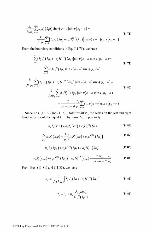
© 200
(11.78)
From the boundary conditions in Eq. (11.75), we have
(11.79)
(11.80)
Since Eqs. (11.77) and (11.80) hold for all , the series on the left and righthand sides should be equal term by term. More precisely,
(11.81)
(11.82)
(11.83)
(11.84)
From Eqs. (11.81) and (11.83), we have
(11.85)
(11.86)
( ) ( ) ( )
( ) ( ) ( )( ) ( ) ( )
11 0
00
20
00
sin sin
sin sin
n vn
n v n νn
k a J k a v φ α v φ αjωµ
k b J ka c H ka v φ α v φ αjωµ
∞
=
∞
=
′ − − =
′′ + − −
∑
∑
( ) ( ) ( )( ) ( ) ( )
( ) ( ) ( ) ( )
20 0 0
0
20 0
0
sin sin
sin sin
n v n νn
n νn
b J kρ c H kρ v φ α v φ α
d H kρ v φ α v φ α
∞
=
∞
=
+ − − =
− −
∑
∑
( ) ( ) ( )( ) ( ) ( )
( ) ( ) ( ) ( )
( ) ( )
20 0 0
00
20 0
00
000
sin sin
sin sin
2 sin sin2
n v n νn
n νn
e
n
k b J kρ c H kρ v φ α v φ αjωµ
k d H kρ v φ α v φ αjωµ
I ν φ α ν φ απ α β ρ
∞
=
∞
=
∞
=
′′ + − − =
′ − −
− − −− −
∑
∑
∑
ϕ
( ) ( ) ( ) ( )21n v n v n νa J k a b J ka c H ka= +
( ) ( ) ( ) ( )( )211
0 0n v n v n ν
k ka J k a b J ka c H kaµ µ
′′ ′= +
( ) ( ) ( ) ( ) ( )2 20 0 0n v n ν n νb J kρ c H kρ d H kρ+ =
( ) ( ) ( ) ( ) ( )2 2 00 0 0
0
22
en v n ν n ν
jη Ib J kρ c H kρ d H kρπ α β ρ
′ ′′ + = −− −
( ) ( ) ( ) ( )2
1
1n n v n v
v
a b J ka c H kaJ k a
= +
( )( ) ( )
02
0
vn n n
v
J kρd c b
H kρ= +
4 by Chapman & Hall/CRC CRC Press LLC
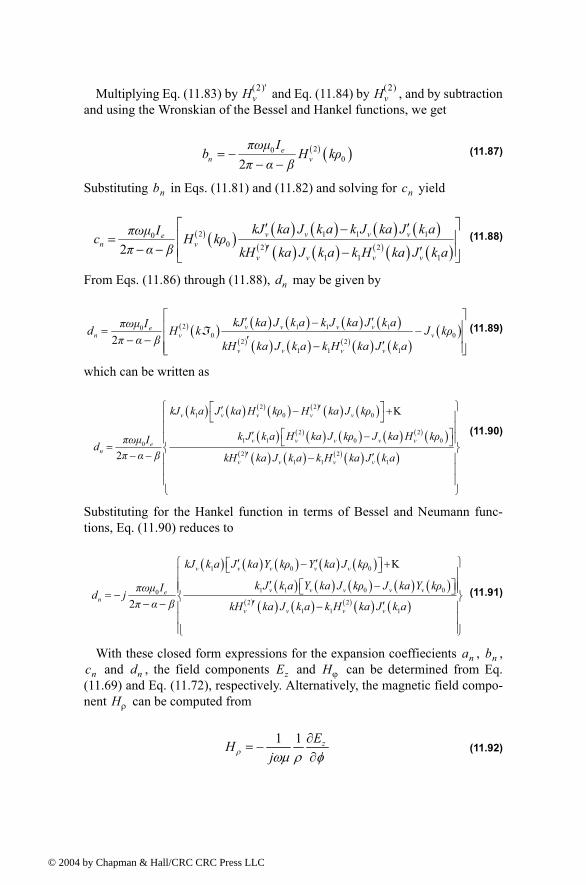
© 200
Multiplying Eq. (11.83) by and Eq. (11.84) by , and by subtractionand using the Wronskian of the Bessel and Hankel functions, we get
(11.87)
Substituting in Eqs. (11.81) and (11.82) and solving for yield
(11.88)
From Eqs. (11.86) through (11.88), may be given by
(11.89)
which can be written as
(11.90)
Substituting for the Hankel function in terms of Bessel and Neumann func-tions, Eq. (11.90) reduces to
(11.91)
With these closed form expressions for the expansion coeffiecients , , and , the field components and can be determined from Eq.
(11.69) and Eq. (11.72), respectively. Alternatively, the magnetic field compo-nent can be computed from
(11.92)
Hv2( )' Hv
2( )
( ) ( )2002
en ν
πωµ Ib H kρ
π α β= −
− −
bn cn
( ) ( ) ( ) ( ) ( ) ( )( ) ( ) ( ) ( ) ( ) ( )
2 1 1 100 2 2
1 1 12
v v v ven ν
ν v ν v
kJ ka J k a k J ka J k aπωµ Ic H kρπ α β kH ka J k a k H ka J k a
′ ′− =
− − ′ ′−
dn
( ) ( ) ( ) ( ) ( ) ( )( ) ( ) ( ) ( ) ( ) ( )
( )2 1 1 100 0
2 21 1 1
2v v v ve
n v v
v v v v
kJ ka J k a k J ka J k aπωµ Id H k J kρπ α β kH ka J k a k H ka J k a
ℑ ′ ′− = − − − ′ ′−
( ) ( ) ( ) ( ) ( ) ( ) ( )
( ) ( ) ( ) ( ) ( ) ( ) ( )( ) ( ) ( ) ( ) ( ) ( )
2 21 0 0
2 21 1 0 002 2
1 1 12
v v ν ν v
v ν v v νen
ν v ν v
kJ k a J ka H kρ H ka J kρ
k J k a H ka J kρ J ka H kρπωµ Idπ α β kH ka J k a k H ka J k a
′′ − + ′ − =
− − ′ ′−
K
( ) ( ) ( ) ( ) ( )( ) ( ) ( ) ( ) ( )
( ) ( ) ( ) ( ) ( ) ( )
1 0 0
1 1 0 002 2
1 1 12
v v ν ν v
v ν v v νen
ν v ν v
kJ k a J ka Y kρ Y ka J kρ
k J k a Y ka J kρ J ka Y kρπωµ Id jπ α β kH ka J k a k H ka J k a
′ ′ − + ′ − = − − − ′ ′−
K
an bncn dn Ez Hϕ
Hρ
1 1 zEHjρ ωµ ρ φ
∂= −
∂
4 by Chapman & Hall/CRC CRC Press LLC
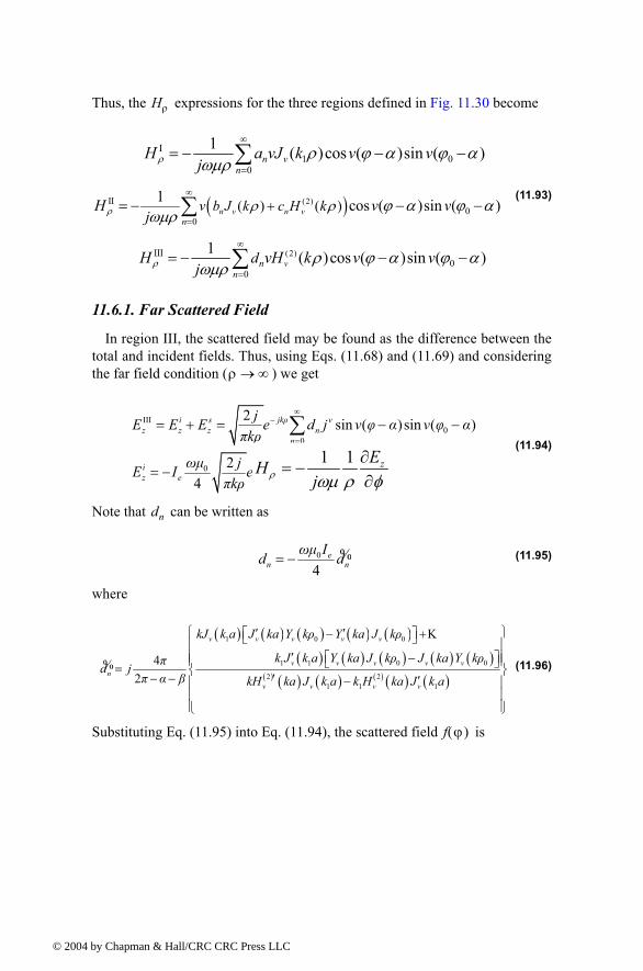
© 200
Thus, the expressions for the three regions defined in Fig. 11.30 become
(11.93)
11.6.1. Far Scattered Field
In region III, the scattered field may be found as the difference between thetotal and incident fields. Thus, using Eqs. (11.68) and (11.69) and consideringthe far field condition ( ) we get
(11.94)
Note that can be written as
(11.95)
where
(11.96)
Substituting Eq. (11.95) into Eq. (11.94), the scattered field is
Hρ
I1 0
0
1 ( )cos ( )sin ( )n vn
H a vJ k v vjρ ρ ϕ α ϕ αωµρ
∞
== − − −∑
( )(2)II0
0( ) ( )1 cos ( )sin ( )n v n v
nv b J k c H kH v v
jρ ρ ρ ϕ α ϕ αωµρ
∞
=+= − − −∑
(2)III0
0
1 ( )cos ( )sin ( )vnn
dH vH k v vjρ ρ ϕ α ϕ αωµρ
∞
== − − −∑
ρ ∞→
( )0 0
III0
0
cos0
2 sin ( )sin ( )
24
i s jkρ vz z z n
n
jkρ φ φi jkρz e
jE E E e d j v φ α v φ απkρ
ωµ jE I e eπkρ
∞−
=
+ −−
= + = − −
= −
∑1 1 zEH
jρ ωµ ρ φ∂
= −∂
dn
0
4e
n nωµ Id d= − %
( ) ( ) ( ) ( ) ( )( ) ( ) ( ) ( ) ( )
( ) ( ) ( ) ( ) ( ) ( )
1 0 0
1 1 0 0
2 21 1 1
42
v v ν ν v
v ν v v νn
ν v ν v
kJ k a J ka Y kρ Y ka J kρ
k J k a Y ka J kρ J ka Y kρπd jπ α β kH ka J k a k H ka J k a
′ ′ − + ′ − = − − ′ ′−
K
%
f ϕ( )
4 by Chapman & Hall/CRC CRC Press LLC
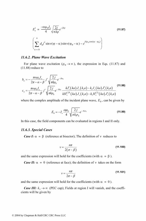
© 200
(11.97)
11.6.2. Plane Wave Excitation
For plane wave excitation ( ), the expression in Eqs. (11.87) and(11.88) reduce to
(11.98)
where the complex amplitude of the incident plane wave, , can be given by
(11.99)
In this case, the field components can be evaluated in regions I and II only.
11.6.3. Special Cases
Case I: (reference at bisector); The definition of reduces to
(11.100)
and the same expression will hold for the coefficients (with ).
Case II: (reference at face); the definition of takes on the form
(11.101)
and the same expression will hold for the coefficients (with ).
Case III: (PEC cap); Fields at region I will vanish, and the coeffi-cients will be given by
Ezs ωµ0Ie
4----------------- 2j
πkρ---------e jkρ
dnjν ν ϕ α( )sin ν ϕ0 α( )sin ejkρ0 ϕ ϕ0( )cos
n 0=
∞
∑
=
ρ0 ∞→
( ) ( ) ( ) ( )( ) ( ) ( ) ( ) ( ) ( )
0
0
0
0
1 1 102 2
0 1 1 1
22
22
jkρνen
v v v vjkρνen
ν v ν v
πωµ I jb j eπ α β πkρ
kJ ka J k a k J ka J k aπωµ I jc j eπ α β πkρ kH ka J k a k H ka J k a
−
−
= −− −
′ ′−=
− − ′ ′−
E0
000
0
24
jke
jE I ek
ρωµπ ρ
−= −
α β= ν
( )2nπνπ β
=−
α β=
α 0= ν
2nπνπ β
=−
α 0=
k1 ∞→
4 by Chapman & Hall/CRC CRC Press LLC
© 200
(11.102)
Note that the expressions of and will yield zero tangential electric fieldat when substituted in Eq.(11.69).
Case IV: (no cap); The expressions of the coefficients in this casemay be obtained by setting , or by taking the limit as approacheszero. Thus,
(11.103)
Case V: and (semi-infinite PEC plane); In this case, thecoefficients in Eq. (11.103) become valid with the exception that the values of
reduce to . Once, the electric field component in the differentregions is computed, the corresponding magnetic field component can becomputed using Eq. (11.71) and the magnetic field component may becomputed as
(11.104)
( ) ( )
( ) ( ) ( )( ) ( )
( ) ( ) ( ) ( )( ) ( )
( ) ( ) ( ) ( )
200
200 2
0 002
2
1
2
2
2
1 0
en ν
ven ν
ν
ν v v νen
ν
n n v n νv
πωµ Ib H kρπ α β
J kaπωµ Ic H kρπ α β H ka
Y ka J kρ J ka Y kρπωµ Id jπ α β H ka
a b J ka c H kaJ k a
= −− −
=− −
−=
− −
= + =
bn cnρ a=
a 0→k1 k= a
( ) ( ) ( ) ( ) ( ) ( )( ) ( ) ( ) ( ) ( ) ( )
( ) ( )
( ) ( ) ( ) ( )
( ) ( ) ( ) ( ) ( ) ( ) ( )
( ) ( ) ( ) ( ) ( )
200 2 2
200
2
2 21 0 0
21 1 00
02
21
2
v v v ven ν
ν v ν v
en ν
n n v n ν nv
v v ν ν v
v ν v ven
kJ ka J ka kJ ka J kaπωµ Ic H kρπ α β kH ka J ka kH ka J ka
πωµ Ib H kρπ α β
a b J ka c H ka bJ ka
kJ k a J ka H kρ H ka J kρ
k J k a H ka J kρ J ka Hπωµ Idπ α β
′ ′− = =
− − ′ ′−
= −− −
= + =
′′ − +
′ −=
− −
K
( ) ( )( ) ( ) ( ) ( ) ( ) ( )
( )
20
2 21 1 1
002
ν
ν v ν v
ev
kρ
kH ka J k a k H ka J k a
πωµ I J kρπ α β
′ ′−
= −− −
a 0→ α β 0= =
v n 2⁄ EzHϕ
Hρ
1 1 zEHjρ ωµ ρ φ
∂= −
∂
4 by Chapman & Hall/CRC CRC Press LLC
© 200
MATLAB Program Capped_WedgeTM.m
The MATLAB program "Capped_WedgeTM.m" given in listing 11.12, alongwith the following associated functions "DielCappedWedgeTMFields_Ls.m",DielCappedWedgeTMFields_PW", "polardb.m", "dbesselj.m", "dbesselh.m",and "dbessely.m" given in the following listings, calculates and plots the farfield of a capped wedge in the presence of an electric line source field. Thenear field distribution is also computed for both line source or plane wave exci-tation. All near field components are computed and displayed, in separate win-dows, using 3-D output format. The program is also capable of analyzing thefield variations due to the cap parameters. The user can execute this MATLABprogram from the MATLAB command window and manually change the inputparameters in the designated section in the program in order to perform thedesired analysis. Alternatively, the "Capped_Wedge_GUI.m" function alongwith the "Capped_Wedge_GUI.fig" file can be used to simplify the data entryprocedure.
A sample of the data entry screen of the "Capped_Wedge_GUI" program isshown in Fig. 11.31 for the case of a line source exciting a sharp conductingwedge. The corresponding far field pattern is shown in Fig. 11.32. When keep-ing all the parameters in Fig. 11.31 the same except that selecting a dielectricor conducting cap, one obtains the far field patterns in Figs. 11.33 and 11.34,respectively. It is clear from these figures how the cap parameters affect thedirection of the maximum radiation of the line source in the presence of thewedge. The distribution of the components of the fields in the near field forthese three cases (sharp edge, dielectric capped edge, and conducting cappededge) is computed and shown in Figs. 11.35 to 11.43. The near field distribu-tion for an incident plane wave field on these three types of wedges is alsocomputed and shown in Figs. 11.44 to 11.52. These near field distributionsclearly demonstrated the effect or cap parameters in altering the sharp edge sin-gular behavior. To further illustrate this effect, the following set of figures(Figs. (11.53) to (11.55)) presents the near field of the electric component ofplane wave incident on a half plane with a sharp edge, dielectric capped edge,and conducting capped edge.
The user is encouraged to experiment with this program as there are manyparameters that can be altered to change the near and far field characteristicdue to the scattering from a wedge structure.
4 by Chapman & Hall/CRC CRC Press LLC
© 200
Figure 11.31. The parameters for computing the far field pattern of a 60 degrees wedge excited by a line source
Figure 11.32. The far field pattern of a line source near a conducting wedge with sharp edge characterized by the parameters in Fig. 11.31.
4 by Chapman & Hall/CRC CRC Press LLC
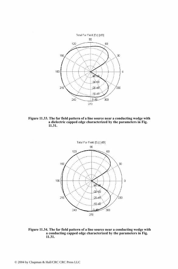
© 200
Figure 11.33. The far field pattern of a line source near a conducting wedge with a dielectric capped edge characterized by the parameters in Fig. 11.31.
Figure 11.34. The far field pattern of a line source near a conducting wedge with a conducting capped edge characterized by the parameters in Fig. 11.31.
4 by Chapman & Hall/CRC CRC Press LLC
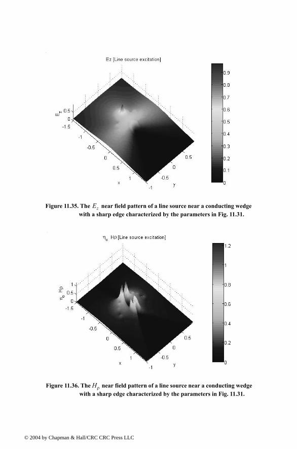
© 200
Figure 11.35. The near field pattern of a line source near a conducting wedge with a sharp edge characterized by the parameters in Fig. 11.31.
Ez
Figure 11.36. The near field pattern of a line source near a conducting wedge with a sharp edge characterized by the parameters in Fig. 11.31.
Hρ
4 by Chapman & Hall/CRC CRC Press LLC
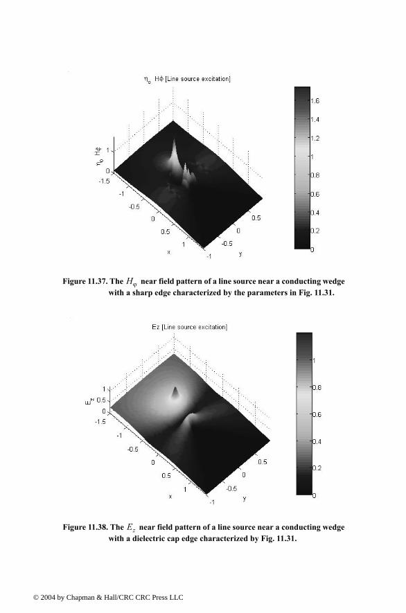
© 200
Figure 11.37. The near field pattern of a line source near a conducting wedge with a sharp edge characterized by the parameters in Fig. 11.31.
Hϕ
Figure 11.38. The near field pattern of a line source near a conducting wedge with a dielectric cap edge characterized by Fig. 11.31.
Ez
4 by Chapman & Hall/CRC CRC Press LLC
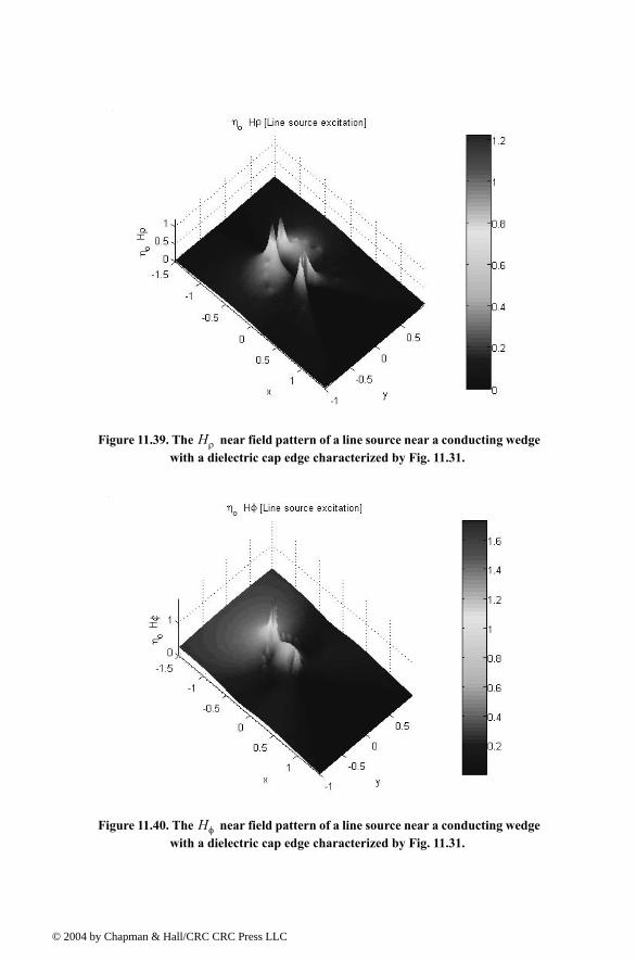
© 200
Figure 11.39. The near field pattern of a line source near a conducting wedge with a dielectric cap edge characterized by Fig. 11.31.
Hρ
Figure 11.40. The near field pattern of a line source near a conducting wedge with a dielectric cap edge characterized by Fig. 11.31.
Hφ
4 by Chapman & Hall/CRC CRC Press LLC
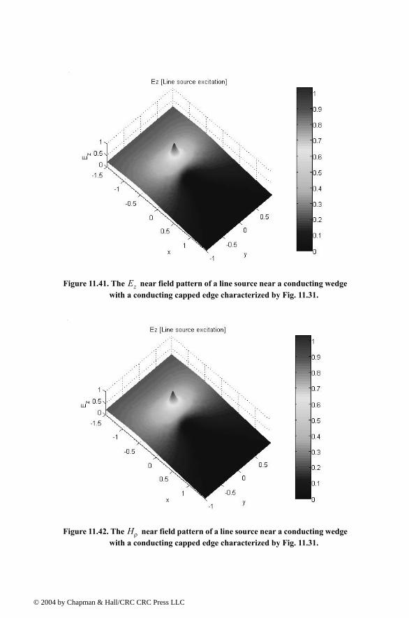
© 200
Figure 11.41. The near field pattern of a line source near a conducting wedge with a conducting capped edge characterized by Fig. 11.31.
Ez
Figure 11.42. The near field pattern of a line source near a conducting wedge with a conducting capped edge characterized by Fig. 11.31.
Hρ
4 by Chapman & Hall/CRC CRC Press LLC
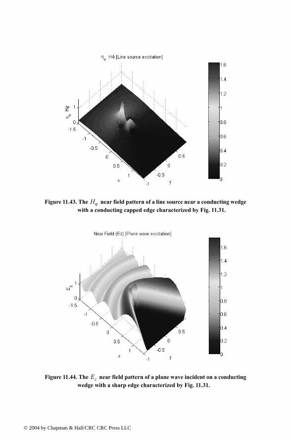
© 200
Figure 11.43. The near field pattern of a line source near a conducting wedge with a conducting capped edge characterized by Fig. 11.31.
Hϕ
Figure 11.44. The near field pattern of a plane wave incident on a conducting wedge with a sharp edge characterized by Fig. 11.31.
Ez
4 by Chapman & Hall/CRC CRC Press LLC
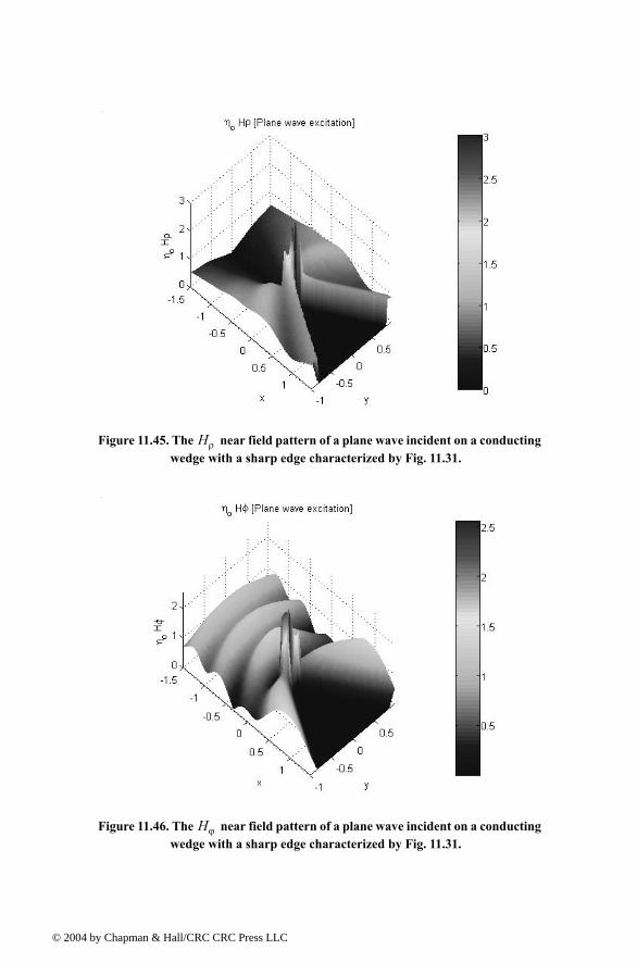
© 200
Figure 11.45. The near field pattern of a plane wave incident on a conducting wedge with a sharp edge characterized by Fig. 11.31.
Hρ
Figure 11.46. The near field pattern of a plane wave incident on a conducting wedge with a sharp edge characterized by Fig. 11.31.
Hϕ
4 by Chapman & Hall/CRC CRC Press LLC
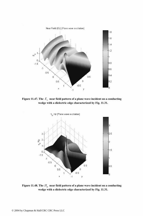
© 200
Figure 11.47. The near field pattern of a plane wave incident on a conducting wedge with a dielectric edge characterized by Fig. 11.31.
Ez
Figure 11.48. The near field pattern of a plane wave incident on a conducting wedge with a dielectric edge characterized by Fig. 11.31.
Hρ
4 by Chapman & Hall/CRC CRC Press LLC
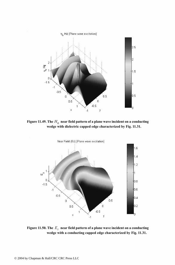
© 200
Figure 11.49. The near field pattern of a plane wave incident on a conducting wedge with dielectric capped edge characterized by Fig. 11.31.
Hϕ
Figure 11.50. The near field pattern of a plane wave incident on a conducting wedge with a conducting capped edge characterized by Fig. 11.31.
Ez
4 by Chapman & Hall/CRC CRC Press LLC
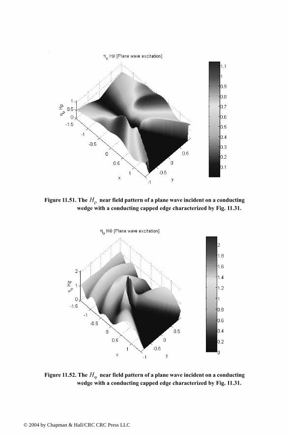
© 200
Figure 11.51. The near field pattern of a plane wave incident on a conducting wedge with a conducting capped edge characterized by Fig. 11.31.
Hρ
Figure 11.52. The near field pattern of a plane wave incident on a conducting wedge with a conducting capped edge characterized by Fig. 11.31.
Hϕ
4 by Chapman & Hall/CRC CRC Press LLC
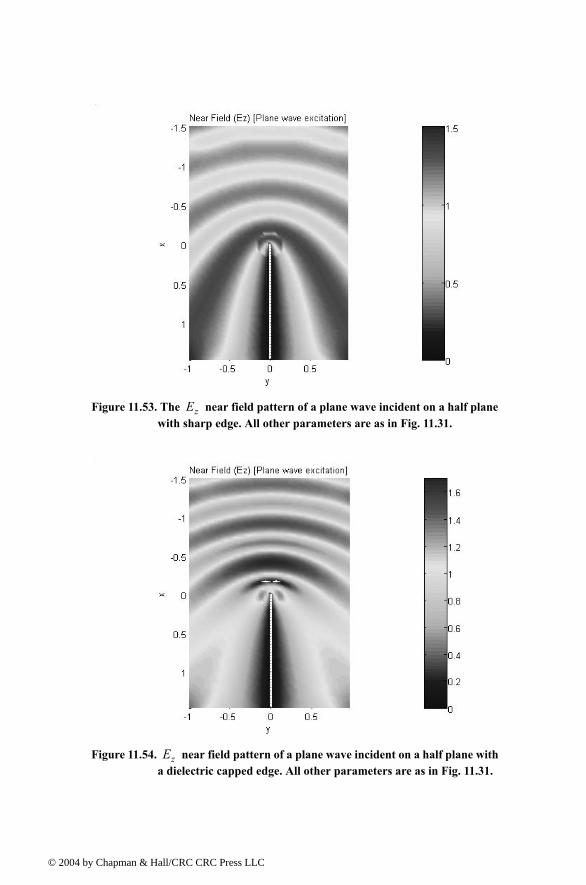
© 200
Figure 11.53. The near field pattern of a plane wave incident on a half plane with sharp edge. All other parameters are as in Fig. 11.31.
Ez
Figure 11.54. near field pattern of a plane wave incident on a half plane with a dielectric capped edge. All other parameters are as in Fig. 11.31.Ez
4 by Chapman & Hall/CRC CRC Press LLC
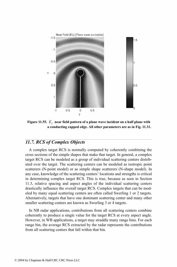
© 200
11.7. RCS of Complex Objects A complex target RCS is normally computed by coherently combining the
cross sections of the simple shapes that make that target. In general, a complextarget RCS can be modeled as a group of individual scattering centers distrib-uted over the target. The scattering centers can be modeled as isotropic pointscatterers (N-point model) or as simple shape scatterers (N-shape model). Inany case, knowledge of the scattering centers locations and strengths is criticalin determining complex target RCS. This is true, because as seen in Section11.3, relative spacing and aspect angles of the individual scattering centersdrastically influence the overall target RCS. Complex targets that can be mod-eled by many equal scattering centers are often called Swerling 1 or 2 targets.Alternatively, targets that have one dominant scattering center and many othersmaller scattering centers are known as Swerling 3 or 4 targets.
In NB radar applications, contributions from all scattering centers combinecoherently to produce a single value for the target RCS at every aspect angle.However, in WB applications, a target may straddle many range bins. For eachrange bin, the average RCS extracted by the radar represents the contributionsfrom all scattering centers that fall within that bin.
Figure 11.55. near field pattern of a plane wave incident on a half plane with a conducting capped edge. All other parameters are as in Fig. 11.31.Ez
4 by Chapman & Hall/CRC CRC Press LLC
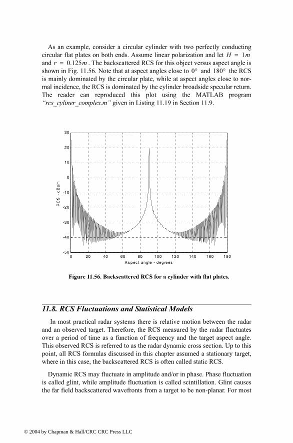
© 200
As an example, consider a circular cylinder with two perfectly conductingcircular flat plates on both ends. Assume linear polarization and let and . The backscattered RCS for this object versus aspect angle isshown in Fig. 11.56. Note that at aspect angles close to and the RCSis mainly dominated by the circular plate, while at aspect angles close to nor-mal incidence, the RCS is dominated by the cylinder broadside specular return.The reader can reproduced this plot using the MATLAB programrcs_cyliner_complex.m given in Listing 11.19 in Section 11.9.
11.8. RCS Fluctuations and Statistical Models In most practical radar systems there is relative motion between the radar
and an observed target. Therefore, the RCS measured by the radar fluctuatesover a period of time as a function of frequency and the target aspect angle.This observed RCS is referred to as the radar dynamic cross section. Up to thispoint, all RCS formulas discussed in this chapter assumed a stationary target,where in this case, the backscattered RCS is often called static RCS.
Dynamic RCS may fluctuate in amplitude and/or in phase. Phase fluctuationis called glint, while amplitude fluctuation is called scintillation. Glint causesthe far field backscattered wavefronts from a target to be non-planar. For most
H 1m=r 0.125m=
0° 180°
Figure 11.56. Backscattered RCS for a cylinder with flat plates.
0 20 40 60 80 100 120 140 160 180-50
-40
-30
-20
-10
0
10
20
30
A s pec t angle - degrees
RC
S -
dB
sm
4 by Chapman & Hall/CRC CRC Press LLC
© 200
radar applications, glint introduces linear errors in the radar measurements, andthus it is not of a major concern. However, in cases where high precision andaccuracy are required, glint can be detrimental. Examples include precisioninstrumentation tracking radar systems, missile seekers, and automated aircraftlanding systems. For more details on glint, the reader is advised to visit citedreferences listed in the bibliography.
Radar cross-section scintillation can vary slowly or rapidly depending on thetarget size, shape, dynamics, and its relative motion with respect to the radar.Thus, due to the wide variety of RCS scintillation sources, changes in the radarcross section are modeled statistically as random processes. The value of anRCS random process at any given time defines a random variable at that time.Many of the RCS scintillation models were developed and verified by experi-mental measurements.
11.8.1. RCS Statistical Models - Scintillation Models
This section presents the most commonly used RCS statistical models. Sta-tistical models that apply to sea, land, and volume clutter, such as the Weibulland Log-normal distributions, will be discussed in a later chapter. The choiceof a particular model depends heavily on the nature of the target under exami-nation.
Chi-Square of Degree
The Chi-square distribution applies to a wide range of targets; its pdf is givenby
(11.105)
where is the gamma function with argument , and is the averagevalue. As the degree gets larger the distribution corresponds to constrainedRCS values (narrow range of values). The limit corresponds to a con-stant RCS target (steady-target case).
Swerling I and II (Chi-Square of Degree 2)
In Swerling I, the RCS samples measured by the radar are correlatedthroughout an entire scan, but are uncorrelated from scan to scan (slow fluctu-ation). In this case, the pdf is
(11.106)
where denotes the average RCS overall target fluctuation. Swerling II tar-get fluctuation is more rapid than Swerling I, but the measurements are pulse to
2m
f σ( ) mΓ m( )σav--------------------- mσ
σav-------- m 1
emσ σav⁄
= σ 0≥
Γ m( ) m σav
m ∞→
f σ( ) 1σav--------
σσav--------
exp= σ 0≥
σav
4 by Chapman & Hall/CRC CRC Press LLC
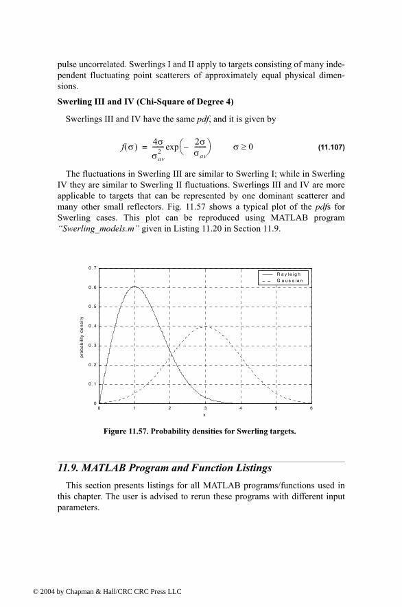
© 200
pulse uncorrelated. Swerlings I and II apply to targets consisting of many inde-pendent fluctuating point scatterers of approximately equal physical dimen-sions.
Swerling III and IV (Chi-Square of Degree 4)
Swerlings III and IV have the same pdf, and it is given by
(11.107)
The fluctuations in Swerling III are similar to Swerling I; while in SwerlingIV they are similar to Swerling II fluctuations. Swerlings III and IV are moreapplicable to targets that can be represented by one dominant scatterer andmany other small reflectors. Fig. 11.57 shows a typical plot of the pdfs forSwerling cases. This plot can be reproduced using MATLAB programSwerling_models.m given in Listing 11.20 in Section 11.9.
11.9. MATLAB Program and Function ListingsThis section presents listings for all MATLAB programs/functions used in
this chapter. The user is advised to rerun these programs with different inputparameters.
f σ( ) 4σσav
2--------
2σσav--------
exp= σ 0≥
Figure 11.57. Probability densities for Swerling targets.
0 1 2 3 4 5 60
0 . 1
0 . 2
0 . 3
0 . 4
0 . 5
0 . 6
0 . 7
x
pro
ba
bili
ty d
en
sit
y
R a y le ig h
G a u s s ia n
4 by Chapman & Hall/CRC CRC Press LLC
© 200
Listing 11.1. MATLAB Function rcs_aspect.mfunction [rcs] = rcs_aspect (scat_spacing, freq)% This function demonstrates the effect of aspect angle on RCS.% Plot scatterers separated by scat_spacing meter. Initially the two scatterers% are aligned with radar line of sight. The aspect angle is changed from% 0 degrees to 180 degrees and the equivalent RCS is computed.% Plot of RCS versus aspect is generated.eps = 0.00001;wavelength = 3.0e+8 / freq;% Compute aspect angle vectoraspect_degrees = 0.:.05:180.;aspect_radians = (pi/180) .* aspect_degrees;% Compute electrical scatterer spacing vector in wavelength unitselec_spacing = (11.0 * scat_spacing / wavelength) .* cos(aspect_radians);% Compute RCS (rcs = RCS_scat1 + RCS_scat2)% Scat1 is taken as phase reference pointrcs = abs(1.0 + cos((11.0 * pi) .* elec_spacing) ... + i * sin((11.0 * pi) .* elec_spacing));rcs = rcs + eps;rcs = 20.0*log10(rcs); % RCS in dBsm % Plot RCS versus aspect anglefigure (1);plot (aspect_degrees,rcs,'k');grid;xlabel ('aspect angle - degrees');ylabel ('RCS in dBsm');%title (' Frequency is 3GHz; scatterer spacing is 0.5m');
Listing 11.2. MATLAB Function rcs_frequency.mfunction [rcs] = rcs_frequency (scat_spacing, frequ, freql)% This program demonstrates the dependency of RCS on wavelength eps = 0.0001;freq_band = frequ - freql;delfreq = freq_band / 500.;index = 0;for freq = freql: delfreq: frequ index = index +1; wavelength(index) = 3.0e+8 / freq;endelec_spacing = 2.0 * scat_spacing ./ wavelength;rcs = abs ( 1 + cos((11.0 * pi) .* elec_spacing) ... + i * sin((11.0 * pi) .* elec_spacing));
4 by Chapman & Hall/CRC CRC Press LLC

© 200
rcs = rcs + eps;rcs = 20.0*log10(rcs); % RCS ins dBsm% Plot RCS versus frequencyfreq = freql:delfreq:frequ;plot(freq,rcs);grid;xlabel('Frequency');ylabel('RCS in dBsm');
Listing 11.3. MATLAB Program example11_1.mclear allclose allN = 50;wct = linspace(0,2*pi,N);% Case 1ax1 = cos(wct);ay1 = sqrt(3) .* cos(wct);M1 = moviein(N);figure(1)xc =0;yc=0;axis imagehold onfor ii = 1:N plot(ax1(ii),ay1(ii),'>r'); line([xc ax1(ii)],[yc ay1(ii)]); plot(ax1,ay1,'g'); M1(ii) = getframe;endgridxlabel('Ex')ylabel('Ey')title('Electric Field Locus; case1')% case 2ax3 = cos(wct);ay3 = sin(wct);M3 = moviein(N);figure(3)axis imagehold onfor ii = 1:N plot(ax3(ii),ay3(ii),'>r'); line([xc ax3(ii)],[yc ay3(ii)]);
4 by Chapman & Hall/CRC CRC Press LLC
© 200
plot(ax3,ay3,'g'); M3(ii) = getframe;endgridxlabel('Ex')ylabel('Ey')title('Electric Field Locus; case 2')rho = sqrt(ax3.^2 + ay3.^2);major_axis = 2*max(rho);minor_axis = 2*min(rho);aspect3 = 10*log10(major_axis/minor_axis)alpha3 = (180/pi) * atan2(ay3(1),ax3(1))% Case 3ax4 = cos(wct);ay4 = cos(wct+(pi/6));M4 = moviein(N);figure(4)axis imagehold onfor ii = 1:N plot(ax4(ii),ay4(ii),'>r'); line([xc ax4(ii)],[yc ay4(ii)]); plot(ax4,ay4,'g') M4(ii) = getframe;endgridxlabel('Ex')ylabel('Ey')title('Electric Field Locus; case 3')rho = sqrt(ax4.^2 + ay4.^2);major_axis = 2*max(rho);minor_axis = 2*min(rho);aspect4 = 10*log10(major_axis/minor_axis)alpha4 = (180/pi) * atan2(ay4(1),ax4(1))end% Case 4ax6 = cos(wct);ay6 = sqrt(3) .* cos(wct+(pi/3));M6 = moviein(N);figure(6)axis image
hold onfor ii = 1:N
4 by Chapman & Hall/CRC CRC Press LLC
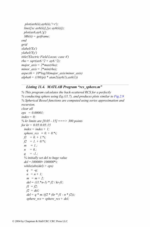
© 200
plot(ax6(ii),ay6(ii),'>r'); line([xc ax6(ii)],[yc ay6(ii)]); plot(ax6,ay6,'g') M6(ii) = getframe;endgridxlabel('Ex')ylabel('Ey')title('Electric Field Locus; case 4')rho = sqrt(ax6.^2 + ay6.^2);major_axis = 2*max(rho);minor_axis = 2*min(rho);aspect6 = 10*log10(major_axis/minor_axis)alpha6 = (180/pi) * atan2(ay6(1),ax6(1))
Listing 11.4. MATLAB Program rcs_sphere.m% This program calculates the back-scattered RCS for a perfectly% conducting sphere using Eq.(11.7), and produces plots similar to Fig.2.9 % Spherical Bessel functions are computed using series approximation and recursion.clear alleps = 0.00001;index = 0;% kr limits are [0.05 - 15] ===> 300 pointsfor kr = 0.05:0.05:15 index = index + 1; sphere_rcs = 0. + 0.*i; f1 = 0. + 1.*i; f2 = 1. + 0.*i; m = 1.; n = 0.; q = -1.; % initially set del to huge value del =100000+100000*i; while(abs(del) > eps) q = -q; n = n + 1; m = m + 2; del = (11.*n-1) * f2 / kr-f1; f1 = f2; f2 = del; del = q * m /(f2 * (kr * f1 - n * f2)); sphere_rcs = sphere_rcs + del;
4 by Chapman & Hall/CRC CRC Press LLC
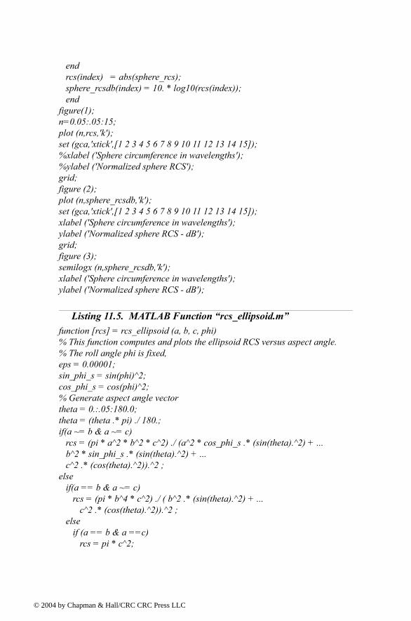
© 200
end rcs(index) = abs(sphere_rcs); sphere_rcsdb(index) = 10. * log10(rcs(index)); endfigure(1);n=0.05:.05:15;plot (n,rcs,'k');set (gca,'xtick',[1 2 3 4 5 6 7 8 9 10 11 12 13 14 15]);%xlabel ('Sphere circumference in wavelengths');%ylabel ('Normalized sphere RCS');grid;figure (2);plot (n,sphere_rcsdb,'k');set (gca,'xtick',[1 2 3 4 5 6 7 8 9 10 11 12 13 14 15]);xlabel ('Sphere circumference in wavelengths');ylabel ('Normalized sphere RCS - dB');grid;figure (3);semilogx (n,sphere_rcsdb,'k');xlabel ('Sphere circumference in wavelengths');ylabel ('Normalized sphere RCS - dB');
Listing 11.5. MATLAB Function rcs_ellipsoid.m function [rcs] = rcs_ellipsoid (a, b, c, phi)% This function computes and plots the ellipsoid RCS versus aspect angle.% The roll angle phi is fixed,eps = 0.00001;sin_phi_s = sin(phi)^2;cos_phi_s = cos(phi)^2;% Generate aspect angle vectortheta = 0.:.05:180.0;theta = (theta .* pi) ./ 180.;if(a ~= b & a ~= c) rcs = (pi * a^2 * b^2 * c^2) ./ (a^2 * cos_phi_s .* (sin(theta).^2) + ... b^2 * sin_phi_s .* (sin(theta).^2) + ... c^2 .* (cos(theta).^2)).^2 ;else if(a == b & a ~= c) rcs = (pi * b^4 * c^2) ./ ( b^2 .* (sin(theta).^2) + ... c^2 .* (cos(theta).^2)).^2 ; else if (a == b & a ==c) rcs = pi * c^2;
4 by Chapman & Hall/CRC CRC Press LLC
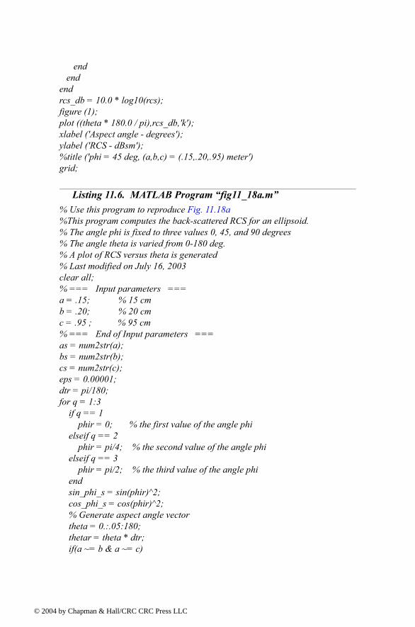
© 200
end endendrcs_db = 10.0 * log10(rcs);figure (1);plot ((theta * 180.0 / pi),rcs_db,'k');xlabel ('Aspect angle - degrees');ylabel ('RCS - dBsm');%title ('phi = 45 deg, (a,b,c) = (.15,.20,.95) meter')grid;
Listing 11.6. MATLAB Program fig11_18a.m% Use this program to reproduce Fig. 11.18a%This program computes the back-scattered RCS for an ellipsoid.% The angle phi is fixed to three values 0, 45, and 90 degrees% The angle theta is varied from 0-180 deg.% A plot of RCS versus theta is generated% Last modified on July 16, 2003clear all;% === Input parameters ===a = .15; % 15 cmb = .20; % 20 cmc = .95 ; % 95 cm% === End of Input parameters ===as = num2str(a);bs = num2str(b);cs = num2str(c);eps = 0.00001;dtr = pi/180;for q = 1:3 if q == 1 phir = 0; % the first value of the angle phi elseif q == 2 phir = pi/4; % the second value of the angle phi elseif q == 3 phir = pi/2; % the third value of the angle phi end sin_phi_s = sin(phir)^2; cos_phi_s = cos(phir)^2; % Generate aspect angle vector theta = 0.:.05:180; thetar = theta * dtr; if(a ~= b & a ~= c)
4 by Chapman & Hall/CRC CRC Press LLC

© 200
rcs(q,:) = (pi * a^2 * b^2 * c^2) ./ (a^2 * cos_phi_s .* (sin(thetar).^2) + ... b^2 * sin_phi_s .* (sin(thetar).^2) + ... c^2 .* (cos(thetar).^2)).^2 ; elseif(a == b & a ~= c) rcs(q,:) = (pi * b^4 * c^2) ./ ( b^2 .* (sin(thetar).^2) + ... c^2 .* (cos(thetar).^2)).^2 ; elseif (a == b & a ==c) rcs(q,:) = pi * c^2; endendrcs_db = 10.0 * log10(rcs);figure (1);plot(theta,rcs_db(1,:),'b',theta,rcs_db(2,:),'r:',theta,rcs_db(3,:),'g--','line-width',1.5);xlabel ('Aspect angle, Theta [Degrees]');ylabel ('RCS - dBsm');title (['Ellipsoid with (a,b,c) = (', [as],', ', [bs],', ', [cs], ') meter'])legend ('phi = 0^o','phi = 45^o','phi = 90^o')grid;
Listing 11.7. MATLAB Function rcs_circ_plate.m function [rcsdb] = rcs_circ_plate (r, freq) % This program calculates and plots the backscattered RCS of% circular flat plate of radius r.eps = 0.000001;% Compute aspect angle vector% Compute wavelengthlambda = 3.e+8 / freq; % X-Bandindex = 0;for aspect_deg = 0.:.1:180 index = index +1; aspect = (pi /180.) * aspect_deg; % Compute RCS using Eq. (2.37) if (aspect == 0 | aspect == pi) rcs_po(index) = (4.0 * pi^3 * r^4 / lambda^2) + eps; rcs_mu(index) = rcs_po(1); else x = (4. * pi * r / lambda) * sin(aspect); val1 = 4. * pi^3 * r^4 / lambda^2; val2 = 2. * besselj(1,x) / x; rcs_po(index) = val1 * (val2 * cos(aspect))^2 + eps;% Compute RCS using Eq. (2.36) val1m = lambda * r;
4 by Chapman & Hall/CRC CRC Press LLC
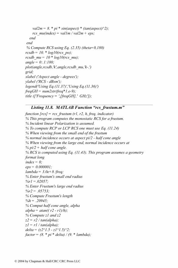
© 200
val2m = 8. * pi * sin(aspect) * (tan(aspect)^2); rcs_mu(index) = val1m / val2m + eps; end end % Compute RCS using Eq. (2.35) (theta=0,180)rcsdb = 10. * log10(rcs_po);rcsdb_mu = 10 * log10(rcs_mu);angle = 0:.1:180;plot(angle,rcsdb,'k',angle,rcsdb_mu,'k-.')grid;xlabel ('Aspect angle - degrees');ylabel ('RCS - dBsm');legend('Using Eq.(11.37)','Using Eq.(11.36)')freqGH = num2str(freq*1.e-9);title (['Frequency = ',[freqGH],' GHz']);
Listing 11.8. MATLAB Function rcs_frustum.mfunction [rcs] = rcs_frustum (r1, r2, h, freq, indicator)% This program computes the monostatic RCS for a frustum.% Incident linear Polarization is assumed.% To compute RCP or LCP RCS one must use Eq. (11.24)% When viewing from the small end of the frustum% normal incidence occurs at aspect pi/2 - half cone angle% When viewing from the large end, normal incidence occurs at% pi/2 + half cone angle.% RCS is computed using Eq. (11.43). This program assumes a geometryformat longindex = 0;eps = 0.000001;lambda = 3.0e+8 /freq;% Enter frustum's small end radius%r1 =.02057;% Enter Frustum's large end radius%r2 = .05753;% Compute Frustum's length%h = .20945;% Comput half cone angle, alphaalpha = atan(( r2 - r1)/h);% Compute z1 and z2z2 = r2 / tan(alpha);z1 = r1 / tan(alpha);delta = (z2^1.5 - z1^1.5)^2;factor = (8. * pi * delta) / (9. * lambda);
4 by Chapman & Hall/CRC CRC Press LLC
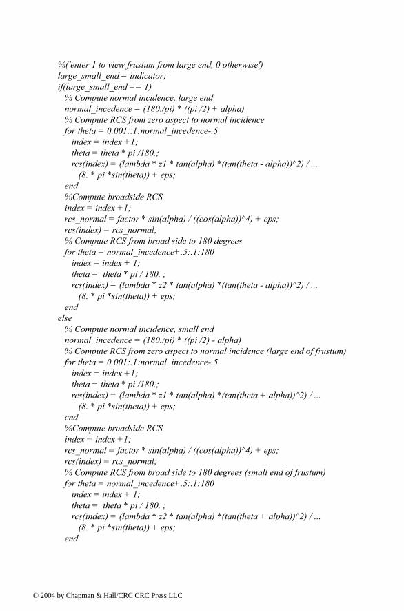
© 200
%('enter 1 to view frustum from large end, 0 otherwise')large_small_end = indicator;if(large_small_end == 1) % Compute normal incidence, large end normal_incedence = (180./pi) * ((pi /2) + alpha) % Compute RCS from zero aspect to normal incidence for theta = 0.001:.1:normal_incedence-.5 index = index +1; theta = theta * pi /180.; rcs(index) = (lambda * z1 * tan(alpha) *(tan(theta - alpha))^2) / ... (8. * pi *sin(theta)) + eps; end %Compute broadside RCS index = index +1; rcs_normal = factor * sin(alpha) / ((cos(alpha))^4) + eps; rcs(index) = rcs_normal; % Compute RCS from broad side to 180 degrees for theta = normal_incedence+.5:.1:180 index = index + 1; theta = theta * pi / 180. ; rcs(index) = (lambda * z2 * tan(alpha) *(tan(theta - alpha))^2) / ... (8. * pi *sin(theta)) + eps; endelse % Compute normal incidence, small end normal_incedence = (180./pi) * ((pi /2) - alpha) % Compute RCS from zero aspect to normal incidence (large end of frustum) for theta = 0.001:.1:normal_incedence-.5 index = index +1; theta = theta * pi /180.; rcs(index) = (lambda * z1 * tan(alpha) *(tan(theta + alpha))^2) / ... (8. * pi *sin(theta)) + eps; end %Compute broadside RCS index = index +1; rcs_normal = factor * sin(alpha) / ((cos(alpha))^4) + eps; rcs(index) = rcs_normal; % Compute RCS from broad side to 180 degrees (small end of frustum) for theta = normal_incedence+.5:.1:180 index = index + 1; theta = theta * pi / 180. ; rcs(index) = (lambda * z2 * tan(alpha) *(tan(theta + alpha))^2) / ... (8. * pi *sin(theta)) + eps; end
4 by Chapman & Hall/CRC CRC Press LLC
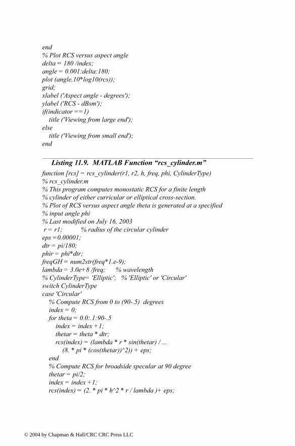
© 200
end% Plot RCS versus aspect angledelta = 180 /index;angle = 0.001:delta:180;plot (angle,10*log10(rcs));grid;xlabel ('Aspect angle - degrees');ylabel ('RCS - dBsm');if(indicator ==1) title ('Viewing from large end');else title ('Viewing from small end');end
Listing 11.9. MATLAB Function rcs_cylinder.mfunction [rcs] = rcs_cylinder(r1, r2, h, freq, phi, CylinderType)% rcs_cylinder.m% This program computes monostatic RCS for a finite length% cylinder of either curricular or elliptical cross-section.% Plot of RCS versus aspect angle theta is generated at a specified % input angle phi% Last modified on July 16, 2003 r = r1; % radius of the circular cylindereps =0.00001;dtr = pi/180;phir = phi*dtr;freqGH = num2str(freq*1.e-9);lambda = 3.0e+8 /freq; % wavelength% CylinderType= 'Elliptic'; % 'Elliptic' or 'Circular' switch CylinderTypecase 'Circular' % Compute RCS from 0 to (90-.5) degrees index = 0; for theta = 0.0:.1:90-.5 index = index +1; thetar = theta * dtr; rcs(index) = (lambda * r * sin(thetar) / ... (8. * pi * (cos(thetar))^2)) + eps; end % Compute RCS for broadside specular at 90 degree thetar = pi/2; index = index +1; rcs(index) = (2. * pi * h^2 * r / lambda )+ eps;
4 by Chapman & Hall/CRC CRC Press LLC
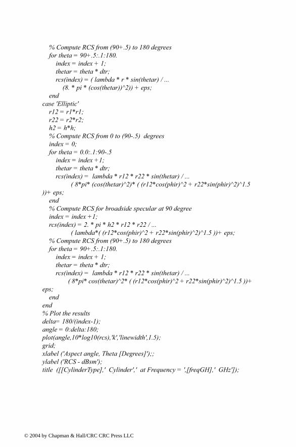
© 200
% Compute RCS from (90+.5) to 180 degrees for theta = 90+.5:.1:180. index = index + 1; thetar = theta * dtr; rcs(index) = ( lambda * r * sin(thetar) / ... (8. * pi * (cos(thetar))^2)) + eps; endcase 'Elliptic' r12 = r1*r1; r22 = r2*r2; h2 = h*h; % Compute RCS from 0 to (90-.5) degrees index = 0; for theta = 0.0:.1:90-.5 index = index +1; thetar = theta * dtr; rcs(index) = lambda * r12 * r22 * sin(thetar) / ... ( 8*pi* (cos(thetar)^2)* ( (r12*cos(phir)^2 + r22*sin(phir)^2)^1.5 ))+ eps; end % Compute RCS for broadside specular at 90 degree index = index +1; rcs(index) = 2. * pi * h2 * r12 * r22 / ... ( lambda*( (r12*cos(phir)^2 + r22*sin(phir)^2)^1.5 ))+ eps; % Compute RCS from (90+.5) to 180 degrees for theta = 90+.5:.1:180. index = index + 1; thetar = theta * dtr; rcs(index) = lambda * r12 * r22 * sin(thetar) / ... ( 8*pi* cos(thetar)^2* ( (r12*cos(phir)^2 + r22*sin(phir)^2)^1.5 ))+ eps; endend% Plot the resultsdelta= 180/(index-1);angle = 0:delta:180;plot(angle,10*log10(rcs),'k','linewidth',1.5);grid;xlabel ('Aspect angle, Theta [Degrees]');;ylabel ('RCS - dBsm');title ([[CylinderType],' Cylinder',' at Frequency = ',[freqGH],' GHz']);
4 by Chapman & Hall/CRC CRC Press LLC
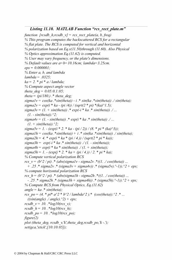
© 200
Listing 11.10. MATLAB Function rcs_rect_plate.mfunction [rcsdb_h,rcsdb_v] = rcs_rect_plate(a, b, freq)% This program computes the backscattered RCS for a rectangular % flat plate. The RCS is computed for vertical and horizontal% polarization based on Eq.s(11.50)through (11.60). Also Physical% Optics approximation Eq.(11.62) is computed.% User may vary frequency, or the plate's dimensions.% Default values are a=b=10.16cm; lambda=3.25cm.eps = 0.000001;% Enter a, b, and lambdalambda = .0325;ka = 2. * pi * a / lambda;% Compute aspect angle vectortheta_deg = 0.05:0.1:85;theta = (pi/180.) .* theta_deg;sigma1v = cos(ka .*sin(theta)) - i .* sin(ka .*sin(theta)) ./ sin(theta);sigma2v = exp(i * ka - (pi /4)) / (sqrt(2 * pi) *(ka)^1.5);sigma3v = (1. + sin(theta)) .* exp(-i * ka .* sin(theta)) ./ ... (1. - sin(theta)).^2;sigma4v = (1. - sin(theta)) .* exp(i * ka .* sin(theta)) ./ ... (1. + sin(theta)).^2;sigma5v = 1. - (exp(i * 2. * ka - (pi / 2)) / (8. * pi * (ka)^3));sigma1h = cos(ka .*sin(theta)) + i .* sin(ka .*sin(theta)) ./ sin(theta);sigma2h = 4. * exp(i * ka * (pi / 4.)) / (sqrt(2 * pi * ka));sigma3h = exp(-i * ka .* sin(theta)) ./ (1. - sin(theta));sigma4h = exp(i * ka * sin(theta)) ./ (1. + sin(theta));sigma5h = 1. - (exp(j * 2. * ka + (pi / 4.)) / 2. * pi * ka);% Compute vertical polarization RCSrcs_v = (b^2 / pi) .* (abs(sigma1v - sigma2v .*((1. ./ cos(theta)) ... + .25 .* sigma2v .* (sigma3v + sigma4v)) .* (sigma5v).^-1)).^2 + eps;% compute horizontal polarization RCSrcs_h = (b^2 / pi) .* (abs(sigma1h - sigma2h .*((1. ./ cos(theta)) ... - .25 .* sigma2h .* (sigma3h + sigma4h)) .* (sigma5h).^-1)).^2 + eps;% Compute RCS from Physical Optics, Eq.(11.62)angle = ka .* sin(theta);rcs_po = (4. * pi* a^2 * b^2 / lambda^2 ).* (cos(theta)).^2 .* ... ((sin(angle) ./ angle).^2) + eps;rcsdb_v = 10. .*log10(rcs_v);rcsdb_h = 10. .*log10(rcs_h);rcsdb_po = 10. .*log10(rcs_po);figure(2)plot (theta_deg, rcsdb_v,'k',theta_deg,rcsdb_po,'k -.');set(gca,'xtick',[10:10:85]);
4 by Chapman & Hall/CRC CRC Press LLC
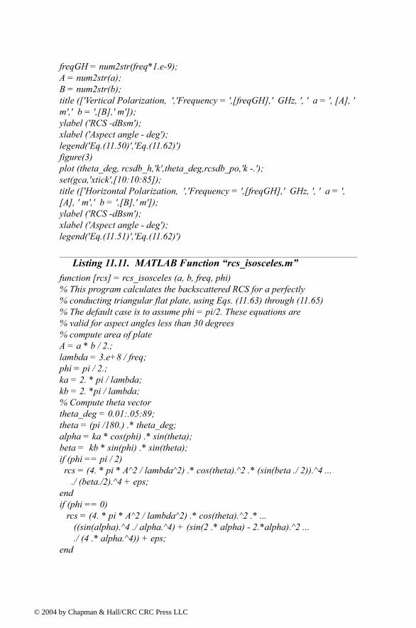
© 200
freqGH = num2str(freq*1.e-9);A = num2str(a);B = num2str(b);title (['Vertical Polarization, ','Frequency = ',[freqGH],' GHz, ', ' a = ', [A], ' m',' b = ',[B],' m']);ylabel ('RCS -dBsm');xlabel ('Aspect angle - deg');legend('Eq.(11.50)','Eq.(11.62)')figure(3)plot (theta_deg, rcsdb_h,'k',theta_deg,rcsdb_po,'k -.');set(gca,'xtick',[10:10:85]);title (['Horizontal Polarization, ','Frequency = ',[freqGH],' GHz, ', ' a = ', [A], ' m',' b = ',[B],' m']);ylabel ('RCS -dBsm');xlabel ('Aspect angle - deg');legend('Eq.(11.51)','Eq.(11.62)')
Listing 11.11. MATLAB Function rcs_isosceles.mfunction [rcs] = rcs_isosceles (a, b, freq, phi)% This program calculates the backscattered RCS for a perfectly% conducting triangular flat plate, using Eqs. (11.63) through (11.65)% The default case is to assume phi = pi/2. These equations are% valid for aspect angles less than 30 degrees% compute area of plateA = a * b / 2.;lambda = 3.e+8 / freq;phi = pi / 2.;ka = 2. * pi / lambda;kb = 2. *pi / lambda;% Compute theta vectortheta_deg = 0.01:.05:89;theta = (pi /180.) .* theta_deg;alpha = ka * cos(phi) .* sin(theta);beta = kb * sin(phi) .* sin(theta);if (phi == pi / 2) rcs = (4. * pi * A^2 / lambda^2) .* cos(theta).^2 .* (sin(beta ./ 2)).^4 ... ./ (beta./2).^4 + eps;endif (phi == 0) rcs = (4. * pi * A^2 / lambda^2) .* cos(theta).^2 .* ... ((sin(alpha).^4 ./ alpha.^4) + (sin(2 .* alpha) - 2.*alpha).^2 ... ./ (4 .* alpha.^4)) + eps;end
4 by Chapman & Hall/CRC CRC Press LLC
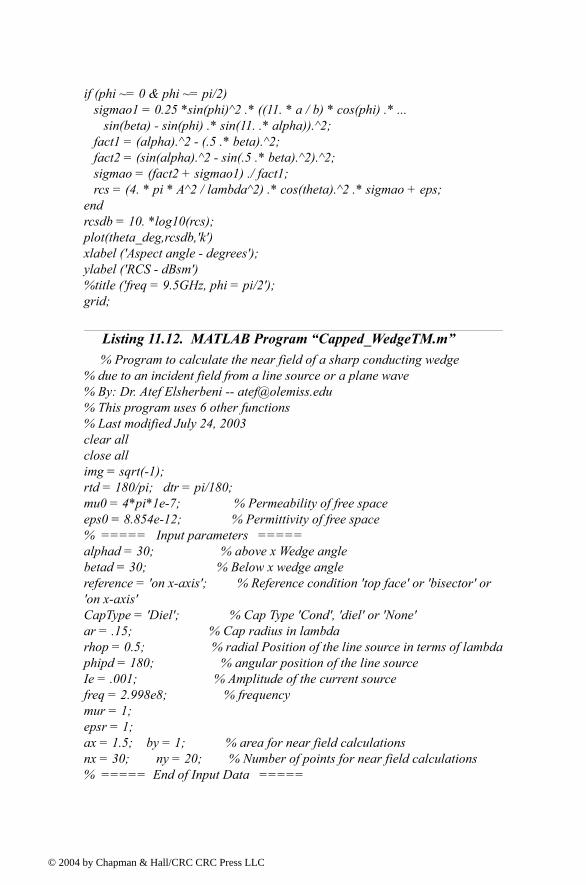
© 200
if (phi ~= 0 & phi ~= pi/2) sigmao1 = 0.25 *sin(phi)^2 .* ((11. * a / b) * cos(phi) .* ... sin(beta) - sin(phi) .* sin(11. .* alpha)).^2; fact1 = (alpha).^2 - (.5 .* beta).^2; fact2 = (sin(alpha).^2 - sin(.5 .* beta).^2).^2; sigmao = (fact2 + sigmao1) ./ fact1; rcs = (4. * pi * A^2 / lambda^2) .* cos(theta).^2 .* sigmao + eps;endrcsdb = 10. *log10(rcs);plot(theta_deg,rcsdb,'k')xlabel ('Aspect angle - degrees');ylabel ('RCS - dBsm')%title ('freq = 9.5GHz, phi = pi/2');grid;
Listing 11.12. MATLAB Program Capped_WedgeTM.m % Program to calculate the near field of a sharp conducting wedge% due to an incident field from a line source or a plane wave % By: Dr. Atef Elsherbeni -- [email protected] % This program uses 6 other functions% Last modified July 24, 2003clear allclose allimg = sqrt(-1);rtd = 180/pi; dtr = pi/180;mu0 = 4*pi*1e-7; % Permeability of free space eps0 = 8.854e-12; % Permittivity of free space % ===== Input parameters =====alphad = 30; % above x Wedge anglebetad = 30; % Below x wedge anglereference = 'on x-axis'; % Reference condition 'top face' or 'bisector' or 'on x-axis'CapType = 'Diel'; % Cap Type 'Cond', 'diel' or 'None'ar = .15; % Cap radius in lambdarhop = 0.5; % radial Position of the line source in terms of lambdaphipd = 180; % angular position of the line source Ie = .001; % Amplitude of the current sourcefreq = 2.998e8; % frequencymur = 1; epsr = 1; ax = 1.5; by = 1; % area for near field calculationsnx = 30; ny = 20; % Number of points for near field calculations% ===== End of Input Data =====
4 by Chapman & Hall/CRC CRC Press LLC
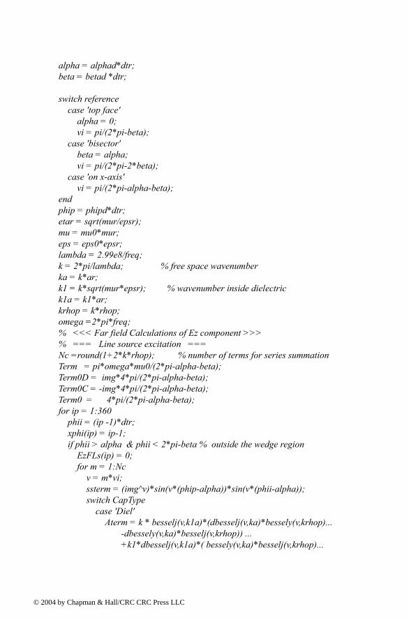
© 200
alpha = alphad*dtr;beta = betad *dtr;
switch reference case 'top face' alpha = 0; vi = pi/(2*pi-beta); case 'bisector' beta = alpha; vi = pi/(2*pi-2*beta); case 'on x-axis' vi = pi/(2*pi-alpha-beta);endphip = phipd*dtr;etar = sqrt(mur/epsr);mu = mu0*mur;eps = eps0*epsr;lambda = 2.99e8/freq;k = 2*pi/lambda; % free space wavenumberka = k*ar;k1 = k*sqrt(mur*epsr); % wavenumber inside dielectrick1a = k1*ar;krhop = k*rhop;omega =2*pi*freq;% <<< Far field Calculations of Ez component >>>% === Line source excitation ===Nc =round(1+2*k*rhop); % number of terms for series summation Term = pi*omega*mu0/(2*pi-alpha-beta);Term0D = img*4*pi/(2*pi-alpha-beta);Term0C = -img*4*pi/(2*pi-alpha-beta);Term0 = 4*pi/(2*pi-alpha-beta);for ip = 1:360 phii = (ip -1)*dtr; xphi(ip) = ip-1; if phii > alpha & phii < 2*pi-beta % outside the wedge region EzFLs(ip) = 0; for m = 1:Nc v = m*vi; ssterm = (img^v)*sin(v*(phip-alpha))*sin(v*(phii-alpha)); switch CapType case 'Diel' Aterm = k * besselj(v,k1a)*(dbesselj(v,ka)*bessely(v,krhop)... -dbessely(v,ka)*besselj(v,krhop)) ... +k1*dbesselj(v,k1a)*( bessely(v,ka)*besselj(v,krhop)...
4 by Chapman & Hall/CRC CRC Press LLC
© 200
-besselj(v,ka)*bessely(v,krhop)); Bterm =k*dbesselh(v,2,ka)*besselj(v,k1a) ... -k1*besselh(v,2,ka)*dbesselj(v,k1a); EzLS(m) = Term0D*ssterm*Aterm/Bterm; case 'Cond' Aterm = bessely(v,ka)*besselj(v,krhop) ... - besselj(v,ka)*bessely(v,krhop); Bterm = besselh(v,2,ka); EzLS(m) = Term0C*ssterm*Aterm/Bterm; case 'None' EzLS(m) = Term0*ssterm*besselj(v,krhop); end end EzFLs(ip) = abs(sum(EzLS)); else EzFLs(ip)=0; endendEzFLs = EzFLs/max(EzFLs);
figure(1);plot(xphi,EzFLs,'linewidth',1.5);xlabel('Observation angle \phi^o'); ylabel('Ez');axis ([0 360 0 1])title('Total Far Field (Ez) [Line source excitation]');
figure(2)polardb(xphi*dtr,EzFLs,'k')title ('Total Far Field (Ez) [dB]')
% <<< Near field observation points >>>delx = 2*ax/nx; dely = 2*by/ny;xi = -ax; yi = -by; % Initial values for x and yfor i = 1:nx for j = 1:ny x(i,j) = xi + (i-1)*delx; y(i,j) = yi + (j-1) *dely; rho(i,j) = sqrt(x(i,j)^2+y(i,j)^2); phi(i,j) = atan2(y(i,j),x(i,j)); if phi(i,j) < 0 phi(i,j) = phi(i,j) + 2*pi; end if rho(i,j) <= 0.001
4 by Chapman & Hall/CRC CRC Press LLC
© 200
rho(i,j) = 0.001; end end end
% Line source excitation, near field calculations
% ==== Line source coefficients ====Nc =round(1+2*k*max(max(rho))); % number of terms for series sum-mation Term = Ie*pi*omega*mu0/(2*pi-alpha-beta);for m = 1:Nc v = m*vi; switch CapType case 'Diel' b(m) = -Term * besselh(v,2,krhop); c(m) = -b(m) * (k*dbesselj(v,ka)*besselj(v,k1a) ... -k1*besselj(v,ka)*dbesselj(v,k1a)) ... /(k*dbesselh(v,2,ka)*besselj(v,k1a) ... -k1*besselh(v,2,ka)*dbesselj(v,k1a)); d(m) = c(m) + b(m) * besselj(v,krhop) ... / besselh(v,2,krhop); a(m) = ( b(m) * besselj(v,ka)+c(m) ... * besselh(v,2,ka))/besselj(v,k1a); case 'Cond' b(m) = -Term * besselh(v,2,krhop); c(m) = -b(m) * besselj(v,ka)/besselh(v,2,ka); d(m) = c(m) + b(m) * besselj(v,krhop) ... / besselh(v,2,krhop); a(m) = 0; case 'None' b(m) = -Term * besselh(v,2,krhop); c(m) = 0; d(m) = -Term * besselj(v,krhop); a(m) = b(m); end end termhphi = sqrt(-1)*omega*mu0;termhrho = -termhphi;for i = 1:nx for j = 1:ny for m = 1:Nc v = m*vi; % Equation
4 by Chapman & Hall/CRC CRC Press LLC
© 200
[Ezt,Hphit,Hrhot] = DielCappedWedgeTMFields_Ls(v,m,rho(i,j),phi(i,j),rhop, ... phip,ar,k,k1,alpha,beta,a,b,c,d); Eztt(m) = Ezt; Hphitt(m) = Hphit; Hrhott(m) = Hrhot; end SEz(i,j) = sum(Eztt); SHphi(i,j) = sum(Hphitt)/termhphi; SHrho(i,j) = sum(Hrhott)/termhrho; endendfigure(3);surf(x,y,abs(SEz));axis ('equal'); view(45,60); shading interp;xlabel('x'); ylabel('y'); zlabel('E_z');title('Ez [Line source excitation]');colorbar; colormap(copper); % colormap(jet);figure(4);surf(x,y,377*abs(SHrho));axis ('equal');view(45,60); shading interp;xlabel('x'); ylabel('y'); zlabel('\eta_o H\rho');title('\eta_o H\rho [Line source excitation]');colorbar; colormap(copper); % colormap(jet);figure(5);surf(x,y,377*abs(SHphi));axis ('equal');view(45,60); shading interp;xlabel('x'); ylabel('y'); zlabel('\eta_o H\phi');title('\eta_o H\phi [Line source excitation]')colorbar; colormap(copper); % colormap(jet);% === Plane wave excitation, near field calculations ===
4 by Chapman & Hall/CRC CRC Press LLC
© 200
Nc =round(1+2*k*max(max(rho))); % number of terms for series sum-mation Term = 4*pi/(2*pi-alpha-beta);for m = 1:Nc v = m*vi; switch CapType case 'Diel' b(m) = Term * img^v; c(m) = -b(m) * (k*dbesselj(v,ka)*besselj(v,k1a)... -k1*besselj(v,ka)*dbesselj(v,k1a)) ... / (k*dbesselh(v,2,ka)*besselj(v,k1a) ... -k1*besselh(v,2,ka)*dbesselj(v,k1a)); a(m) = ( b(m) * besselj(v,ka)+c(m) * besselh(v,2,ka))/besselj(v,k1a); case 'Cond' b(m) = -Term * img^v; c(m) = -b(m) * besselj(v,ka)/besselh(v,2,ka); a(m) = 0; case 'None' b(m) = -Term * img^v; c(m) = 0; a(m) = b(m); end endtermhphi = sqrt(-1)*omega*mu0;termhrho = -termhphi;for i = 1:nx for j = 1:ny for m = 1:Nc v = m*vi; % Equation [Ezt,Hphit,Hrhot] = DielCappedWedgeTMFields_PW(v,m,rho(i,j),phi(i,j), ... phip,ar,k,k1,alpha,beta,a,b,c); Eztt(m) = Ezt; Hphitt(m) = Hphit; Hrhott(m) = Hrhot;end EzPW(i,j) = sum(Eztt); HphiPW(i,j) = sum(Hphitt)/termhphi; HrhoPW(i,j) = sum(Hrhott)/termhrho; endend figure(6);surf(x,y,abs(EzPW));axis ('equal');
4 by Chapman & Hall/CRC CRC Press LLC
© 200
view(45,60); shading interp;xlabel('x'); ylabel('y'); zlabel('E_z');colorbar; colormap(copper); % colormap(jet);title('Near Field (Ez) [Plane wave excitation]');figure(7);surf(x,y,377*abs(HrhoPW));axis ('equal');view(45,60); shading interp;xlabel('x'); ylabel('y'); zlabel('\eta_o H\rho');title('\eta_o H\rho [Plane wave excitation]');colorbar; colormap(copper); % colormap(jet);figure(8);surf(x,y,377*abs(HphiPW));axis ('equal');view(45,60); shading interp;xlabel('x'); ylabel('y'); zlabel('\eta_o H\phi');title('\eta_o H\phi [Plane wave excitation]');colorbar; colormap(copper); % colormap(jet);
Listing 11.13. MATLAB Function "DielCappedWedgeTMFields_Ls.m"
function [Ezt,Hphit,Hrhot] = DielCappedWedgeTMFields_Ls(v,m,rhoij,phiij,rhop,phip,ar,k,k1,alpha,beta,a,b,c,d);% Function to calculate the near field components of a capped wedge % with a line source excitation at one near field point% This function is to be called by the Main program: Diel_Capped_WedgeTM.m% By: Dr. Atef Elsherbeni -- [email protected] % Last modified July 23, 2003Ezt = 0; Hrhot = 0; Hphit = 0; % Initializationif phiij > alpha & phiij < 2*pi-beta % outside the wedge region krho = k*rhoij; k1rho = k1*rhoij;
4 by Chapman & Hall/CRC CRC Press LLC
© 200
jvkrho = besselj(v,krho); hvkrho = besselh(v,2,krho); jvk1rho = besselj(v,k1rho); djvkrho = dbesselj(v,krho); djvk1rho = dbesselj(v,k1rho); dhvkrho = dbesselh(v,2,krho); ssterm = sin(v*(phip-alpha))*sin(v*(phiij-alpha)); scterm = sin(v*(phip-alpha))*cos(v*(phiij-alpha)); if rhoij <= ar % field point location is inside the cap region Ezt = a(m)*jvk1rho*ssterm; Hphit = k1*a(m)*djvk1rho*ssterm; Hrhot = v*a(m)*jvk1rho*scterm/rhoij; elseif rhoij <= rhop % field point location is between cap and the line source location Ezt = (b(m)*jvkrho+c(m)*hvkrho)*ssterm; Hphit = k*(b(m)*djvkrho+c(m)*dhvkrho)*ssterm; Hrhot = v*(b(m)*jvkrho+c(m)*hvkrho)*scterm/rhoij; elseif rhoij > rhop % field point location is greater than the line source loca-tion Ezt = d(m)*hvkrho*ssterm; Hphit = k*d(m)*dhvkrho*ssterm; Hrhot = v*d(m)*hvkrho*scterm/rhoij; endelse Ezt = 0; Hrhot = 0; Hphit = 0; % inside wedge regionEnd
Listing 11.14. MATLAB Function "DielCappedWedgeTMFields_PW.m"
function [Ezt,Hphit,Hrhot] = DielCappedWedgeTMFields_PW(v,m,rhoij,phiij,phip,ar,k,k1,alpha,beta,a,b,c);% Function to calculate the near field components of a capped wedge % with a line source excitation at one near field point% This function is to be called by the Main program: Diel_Capped_WedgeTM.m% By: Dr. Atef Elsherbeni -- [email protected] % Last modified July 23, 2003Ezt = 0; Hrhot = 0; Hphit = 0; % Initializationif phiij > alpha & phiij < 2*pi-beta % outside the wedge region krho = k*rhoij; k1rho = k1*rhoij; jvkrho = besselj(v,krho);
4 by Chapman & Hall/CRC CRC Press LLC
© 200
hvkrho = besselh(v,2,krho); jvk1rho = besselj(v,k1rho); djvkrho = dbesselj(v,krho); djvk1rho = dbesselj(v,k1rho); dhvkrho = dbesselh(v,2,krho); ssterm = sin(v*(phip-alpha))*sin(v*(phiij-alpha)); scterm = sin(v*(phip-alpha))*cos(v*(phiij-alpha)); if rhoij <= ar % field point location is inside the cap region Ezt = a(m)*jvk1rho*ssterm; Hphit = k1*a(m)*djvk1rho*ssterm; Hrhot = v*a(m)*jvk1rho*scterm/rhoij; else % field point location is between the cap and the line source location Ezt = (b(m)*jvkrho+c(m)*hvkrho)*ssterm; Hphit = k*(b(m)*djvkrho+c(m)*dhvkrho)*ssterm; Hrhot = v*(b(m)*jvkrho+c(m)*hvkrho)*scterm/rhoij; endelse Ezt = 0; Hrhot = 0; Hphit = 0; % inside wedge regionEnd
Listing 11.15. MATLAB Function "polardb.m"function polardb(theta,rho,line_style)% POLARDB Polar coordinate plot.% POLARDB(THETA, RHO) makes a plot using polar coordinates of% the angle THETA, in radians, versus the radius RHO in dB.% The maximum value of RHO should not exceed 1. It should not be% normalized, however (i.e., its max. value may be less than 1).% POLAR(THETA,RHO,S) uses the linestyle specified in string S.% See PLOT for a description of legal linestyles.if nargin < 1 error('Requires 2 or 3 input arguments.')elseif nargin == 2 if isstr(rho) line_style = rho; rho = theta; [mr,nr] = size(rho); if mr == 1 theta = 1:nr; else th = (1:mr)'; theta = th(:,ones(1,nr)); end else
4 by Chapman & Hall/CRC CRC Press LLC
© 200
line_style = 'auto'; endelseif nargin == 1 line_style = 'auto'; rho = theta; [mr,nr] = size(rho); if mr == 1 theta = 1:nr; else th = (1:mr)'; theta = th(:,ones(1,nr)); endendif isstr(theta) | isstr(rho) error('Input arguments must be numeric.');endif ~isequal(size(theta),size(rho)) error('THETA and RHO must be the same size.');end% get hold statecax = newplot;next = lower(get(cax,'NextPlot'));hold_state = ishold;% get x-axis text color so grid is in same colortc = get(cax,'xcolor');ls = get(cax,'gridlinestyle');% Hold on to current Text defaults, reset them to the% Axes' font attributes so tick marks use them.fAngle = get(cax, 'DefaultTextFontAngle');fName = get(cax, 'DefaultTextFontName');fSize = get(cax, 'DefaultTextFontSize');fWeight = get(cax, 'DefaultTextFontWeight');fUnits = get(cax, 'DefaultTextUnits');set(cax, 'DefaultTextFontAngle', get(cax, 'FontAngle'), ... 'DefaultTextFontName', get(cax, 'FontName'), ... 'DefaultTextFontSize', get(cax, 'FontSize'), ... 'DefaultTextFontWeight', get(cax, 'FontWeight'), ... 'DefaultTextUnits','data')% make a radial grid hold on; maxrho =1; hhh=plot([-maxrho -maxrho maxrho maxrho],[-maxrho maxrho maxrho -maxrho]); set(gca,'dataaspectratio',[1 1 1],'plotboxaspectratiomode','auto')
4 by Chapman & Hall/CRC CRC Press LLC
© 200
v = [get(cax,'xlim') get(cax,'ylim')]; ticks = sum(get(cax,'ytick')>=0); delete(hhh);% check radial limits and ticks rmin = 0; rmax = v(4); rticks = max(ticks-1,2); if rticks > 5 % see if we can reduce the number if rem(rticks,2) == 0 rticks = rticks/2; elseif rem(rticks,3) == 0 rticks = rticks/3; end end% only do grids if hold is offif ~hold_state% define a circle th = 0:pi/50:2*pi; xunit = cos(th); yunit = sin(th);% now really force points on x/y axes to lie on them exactly inds = 1:(length(th)-1)/4:length(th); xunit(inds(2:2:4)) = zeros(2,1); yunit(inds(1:2:5)) = zeros(3,1);% plot background if necessary if ~isstr(get(cax,'color')), patch('xdata',xunit*rmax,'ydata',yunit*rmax, ... 'edgecolor',tc,'facecolor',get(gca,'color'),... 'handlevisibility','off'); end% draw radial circles with dB ticks c82 = cos(82*pi/180); s82 = sin(82*pi/180); rinc = (rmax-rmin)/rticks; tickdB=-10*(rticks-1); % the innermost tick dB value for i=(rmin+rinc):rinc:rmax hhh = plot(xunit*i,yunit*i,ls,'color',tc,'linewidth',1,... 'handlevisibility','off'); text((i+rinc/20)*c82*0,-(i+rinc/20)*s82, ... [' ' num2str(tickdB) ' dB'],'verticalalignment','bottom',... 'handlevisibility','off') tickdB=tickdB+10; end set(hhh,'linestyle','-') % Make outer circle solid% plot spokes th = (1:6)*2*pi/12;
4 by Chapman & Hall/CRC CRC Press LLC
© 200
cst = cos(th); snt = sin(th); cs = [-cst; cst]; sn = [-snt; snt]; plot(rmax*cs,rmax*sn,ls,'color',tc,'linewidth',1,... 'handlevisibility','off')% annotate spokes in degrees rt = 1.1*rmax; for i = 1:length(th) text(rt*cst(i),rt*snt(i),int2str(i*30),... 'horizontalalignment','center',... 'handlevisibility','off'); if i == length(th) loc = int2str(0); else loc = int2str(180+i*30); end text(-rt*cst(i),-rt*snt(i),loc,'horizontalalignment','center',... 'handlevisibility','off') end% set view to 2-D view(2);% set axis limits axis(rmax*[-1 1 -1.15 1.15]);end% Reset defaults.set(cax, 'DefaultTextFontAngle', fAngle , ... 'DefaultTextFontName', fName , ... 'DefaultTextFontSize', fSize, ... 'DefaultTextFontWeight', fWeight, ... 'DefaultTextUnits',fUnits );% Tranfrom data to dB scalermin = 0; rmax=1;rinc = (rmax-rmin)/rticks;rhodb=zeros(1,length(rho));for i=1:length(rho) if rho(i)==0 rhodb(i)=0; else rhodb(i)=rmax+2*log10(rho(i))*rinc; end if rhodb(i)<=0 rhodb(i)=0; endend
4 by Chapman & Hall/CRC CRC Press LLC

© 200
% transform data to Cartesian coordinates.xx = rhodb.*cos(theta);yy = rhodb.*sin(theta);% plot data on top of gridif strcmp(line_style,'auto') q = plot(xx,yy);else q = plot(xx,yy,line_style,'linewidth',1.5);endif nargout > 0 hpol = q;endif ~hold_state set(gca,'dataaspectratio',[1 1 1]), axis off; set(cax,'NextPlot',next);endset(get(gca,'xlabel'),'visible','on')set(get(gca,'ylabel'),'visible','on')
Listing 11.16. MATLAB Function "dbesselj.m"function [ res ] = dbesselj( nu,z )res=besselj(nu-1,z)-besselj(nu,z)*nu/z;
Listing 11.17. MATLAB Function "dbessely.m"function [ res ] = dbessely( nu,z )res=bessely(nu-1,z)-bessely(nu,z)*nu/z;
Listing 11.18. MATLAB Function "dbesselh.m"function [ res ] = dbesselh(nu,kind,z)res=besselh(nu-1,kind,z)-besselh(nu,kind,z)*nu/z;
Listing 11.19. MATLAB Program rcs_cylinder_complex.m% This program computes the backscattered RCS for a cylinder% with flat plates.clear allindex = 0;eps =0.00001;a1 =.125;h = 1.;lambda = 3.0e+8 /9.5e+9;lambda = 0.00861;index = 0;
4 by Chapman & Hall/CRC CRC Press LLC
© 200
for theta = 0.0:.1:90-.1 index = index +1; theta = theta * pi /180.; rcs(index) = (lambda * a1 * sin(theta) / ... (8 * pi * (cos(theta))^2)) + eps;endtheta*180/pi;theta = pi/2;index = index +1;rcs(index) = (2 * pi * h^2 * a1 / lambda )+ eps;for theta = 90+.1:.1:180. index = index + 1; theta = theta * pi / 180.; rcs(index) = ( lambda * a1 * sin(theta) / ... (8 * pi * (cos(theta))^2)) + eps;endr = a1;index = 0;for aspect_deg = 0.:.1:180 index = index +1; aspect = (pi /180.) * aspect_deg; % Compute RCS using Eq. (11.37) if (aspect == 0 | aspect == pi) rcs_po(index) = (4.0 * pi^3 * r^4 / lambda^2) + eps; rcs_mu(index) = rcs_po(1); else x = (4. * pi * r / lambda) * sin(aspect); val1 = 4. * pi^3 * r^4 / lambda^2; val2 = 2. * besselj(1,x) / x; rcs_po(index) = val1 * (val2 * cos(aspect))^2 + eps; end endrcs_t =(rcs_po + rcs);angle = 0:.1:180;plot(angle,10*log10(rcs_t(1:1801)),'k');grid;xlabel ('Aspect angle -degrees');ylabel ('RCS -dBsm');
Listing 11.20. MATLAB Program Swerling_models.m% This program computes and plots Swerling statistical models% sigma_bar = 1.5; clear all
4 by Chapman & Hall/CRC CRC Press LLC

© 200
sigma = 0:0.001:6;sigma_bar = 1.5;swer_3_4 = (4. / sigma_bar^2) .* sigma .* ... exp(-2. * (sigma ./ sigma_bar));%t.*exp(-(t.^2)./2.swer_1_2 = (1. /sigma_bar) .* exp( -sigma ./ sigma_bar);plot(sigma,swer_1_2,'k',sigma,swer_3_4,'k');grid;gtext ('Swerling I,II');gtext ('Swerling III,IV');xlabel ('sigma');ylabel ('Probability density');title ('sigma-bar = 1.5');
4 by Chapman & Hall/CRC CRC Press LLC
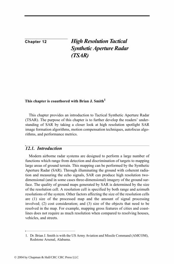
© 200
Chapter 12 High Resolution Tactical Synthetic Aperture Radar (TSAR)
This chapter is coauthored with Brian J. Smith1
This chapter provides an introduction to Tactical Synthetic Aperture Radar (TSAR). The purpose of this chapter is to further develop the readers under-standing of SAR by taking a closer look at high resolution spotlight SAR image formation algorithms, motion compensation techniques, autofocus algo-rithms, and performance metrics.
12.1. IntroductionModern airborne radar systems are designed to perform a large number of
functions which range from detection and discrimination of targets to mapping large areas of ground terrain. This mapping can be performed by the Synthetic Aperture Radar (SAR). Through illuminating the ground with coherent radia-tion and measuring the echo signals, SAR can produce high resolution two-dimensional (and in some cases three-dimensional) imagery of the ground sur-face. The quality of ground maps generated by SAR is determined by the size of the resolution cell. A resolution cell is specified by both range and azimuth resolutions of the system. Other factors affecting the size of the resolution cells are (1) size of the processed map and the amount of signal processing involved; (2) cost consideration; and (3) size of the objects that need to be resolved in the map. For example, mapping gross features of cities and coast-lines does not require as much resolution when compared to resolving houses, vehicles, and streets.
1. Dr. Brian J. Smith is with the US Army Aviation and Missile Command (AMCOM), Redstone Arsenal, Alabama.
4 by Chapman & Hall/CRC CRC Press LLC
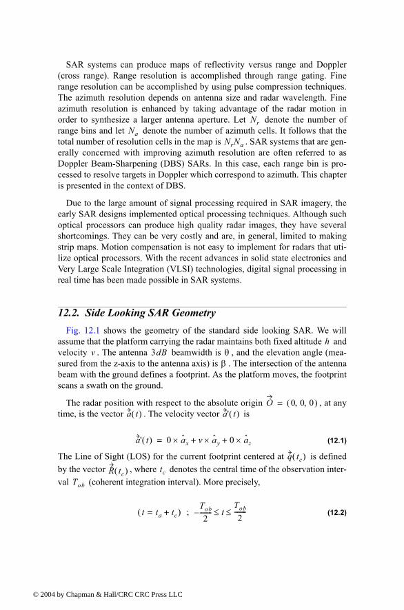
© 200
SAR systems can produce maps of reflectivity versus range and Doppler (cross range). Range resolution is accomplished through range gating. Fine range resolution can be accomplished by using pulse compression techniques. The azimuth resolution depends on antenna size and radar wavelength. Fine azimuth resolution is enhanced by taking advantage of the radar motion in order to synthesize a larger antenna aperture. Let denote the number of range bins and let denote the number of azimuth cells. It follows that the total number of resolution cells in the map is . SAR systems that are gen-erally concerned with improving azimuth resolution are often referred to as Doppler Beam-Sharpening (DBS) SARs. In this case, each range bin is pro-cessed to resolve targets in Doppler which correspond to azimuth. This chapter is presented in the context of DBS.
Due to the large amount of signal processing required in SAR imagery, the early SAR designs implemented optical processing techniques. Although such optical processors can produce high quality radar images, they have several shortcomings. They can be very costly and are, in general, limited to making strip maps. Motion compensation is not easy to implement for radars that uti-lize optical processors. With the recent advances in solid state electronics and Very Large Scale Integration (VLSI) technologies, digital signal processing in real time has been made possible in SAR systems.
12.2. Side Looking SAR GeometryFig. 12.1 shows the geometry of the standard side looking SAR. We will
assume that the platform carrying the radar maintains both fixed altitude and velocity . The antenna beamwidth is , and the elevation angle (mea-sured from the z-axis to the antenna axis) is . The intersection of the antenna beam with the ground defines a footprint. As the platform moves, the footprint scans a swath on the ground.
The radar position with respect to the absolute origin , at any time, is the vector . The velocity vector is
(12.1)
The Line of Sight (LOS) for the current footprint centered at is defined by the vector , where denotes the central time of the observation inter-val (coherent integration interval). More precisely,
(12.2)
NrNa
NrNa
hv 3dB θ
β
O 0 0 0, ,( )=a t( ) a' t( )
a' t( ) 0 a x× v a y× 0 a z×+ +=
q tc( )
R tc( ) tcTob
t ta tc+=( )Tob
2-------- t
Tob
2--------≤ ≤;
4 by Chapman & Hall/CRC CRC Press LLC
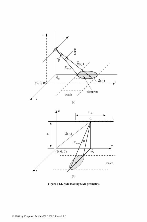
© 200
swath
Figure 12.1. Side looking SAR geometry.
-y
Tob
x
z
h
swath
θ
mg
y
footprint
θ2---
β
0 0 0, ,( ) q tc( )
v
Rmin
R tc( )
mg
a tc( )
x
z
Rmax
tc
(a)
(b)
v
0 0 0, ,( )
4 by Chapman & Hall/CRC CRC Press LLC
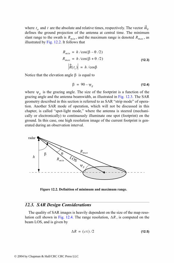
© 200
where and are the absolute and relative times, respectively. The vector defines the ground projection of the antenna at central time. The minimum slant range to the swath is , and the maximum range is denoted , as illustrated by Fig. 12.2. It follows that
(12.3)
Notice that the elevation angle is equal to
(12.4)
where is the grazing angle. The size of the footprint is a function of the grazing angle and the antenna beamwidth, as illustrated in Fig. 12.3. The SAR geometry described in this section is referred to as SAR strip mode of opera-tion. Another SAR mode of operation, which will not be discussed in this chapter, is called spot-light mode, where the antenna is steered (mechani-cally or electronically) to continuously illuminate one spot (footprint) on the ground. In this case, one high resolution image of the current footprint is gen-erated during an observation interval.
12.3. SAR Design ConsiderationsThe quality of SAR images is heavily dependent on the size of the map reso-
lution cell shown in Fig. 12.4. The range resolution, , is computed on the beam LOS, and is given by
(12.5)
ta t mg
Rmin Rmax
Rmin h β θ 2⁄( )cos⁄=
Rmax h β θ 2⁄+( )cos⁄=
R tc( ) h βcos⁄=
β
β 90 ψg=
ψg
Figure 12.2. Definition of minimum and maximum range.
LOSθ Rmax
Rminh
β
ψg
radar
∆R
∆R cτ( ) 2⁄=
4 by Chapman & Hall/CRC CRC Press LLC
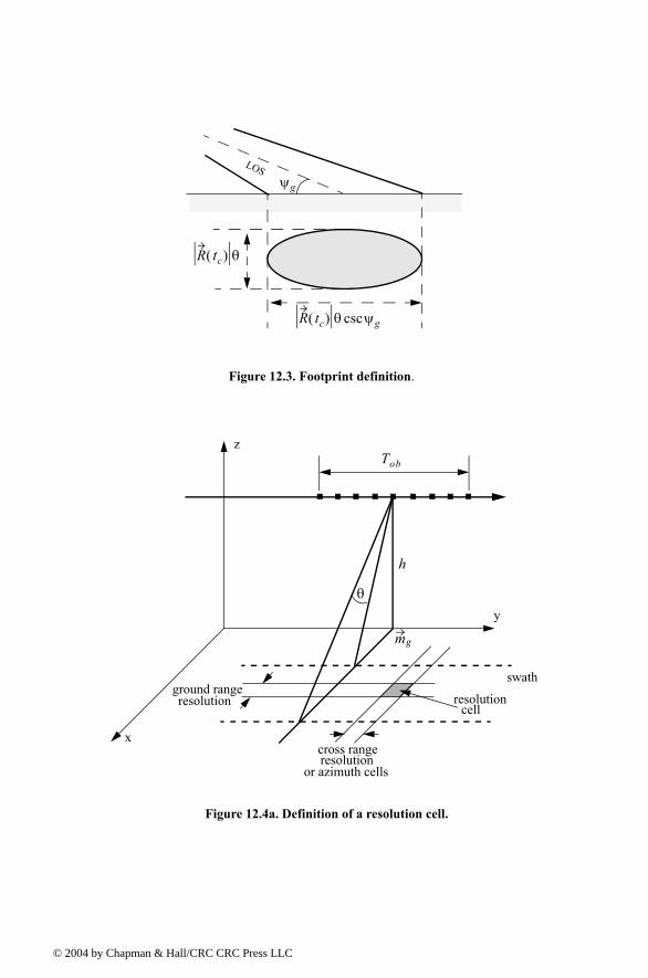
© 200
R tc( ) θ
R tc( ) θ ψgcsc
ψg
Figure 12.3. Footprint definition.
LOS
Tob
Figure 12.4a. Definition of a resolution cell.
x
z
h
swath
θ
mg
resolutioncell
y
ground rangeresolution
cross rangeresolution
or azimuth cells
4 by Chapman & Hall/CRC CRC Press LLC
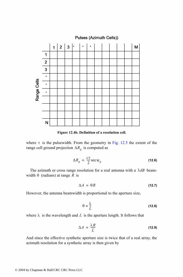
© 200
where is the pulsewidth. From the geometry in Fig. 12.5 the extent of the range cell ground projection is computed as
(12.6)
The azimuth or cross range resolution for a real antenna with a beam-width (radians) at range is
(12.7)
However, the antenna beamwidth is proportional to the aperture size,
(12.8)
where is the wavelength and is the aperture length. It follows that
(12.9)
And since the effective synthetic aperture size is twice that of a real array, the azimuth resolution for a synthetic array is then given by
Figure 12.4b. Definition of a resolution cell.
Pulses (Azimuth Cells))
1 2 3 M
Ran
ge C
ells
1
2
3
N
.
.
.
. . . Pulses (Azimuth Cells))
1 2 3 M
Ran
ge C
ells
1
2
3
N
.
.
.
. . .
τ∆Rg
∆Rgcτ2----- ψgsec=
3dBθ R
∆A θR=
θ λL---≈
λ L
∆A λRL
-------=
4 by Chapman & Hall/CRC CRC Press LLC
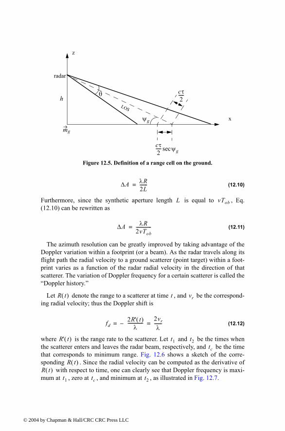
© 200
(12.10)
Furthermore, since the synthetic aperture length is equal to , Eq. (12.10) can be rewritten as
(12.11)
The azimuth resolution can be greatly improved by taking advantage of the Doppler variation within a footprint (or a beam). As the radar travels along its flight path the radial velocity to a ground scatterer (point target) within a foot-print varies as a function of the radar radial velocity in the direction of that scatterer. The variation of Doppler frequency for a certain scatterer is called the Doppler history.
Let denote the range to a scatterer at time , and be the correspond-ing radial velocity; thus the Doppler shift is
(12.12)
where is the range rate to the scatterer. Let and be the times when the scatterer enters and leaves the radar beam, respectively, and be the time that corresponds to minimum range. Fig. 12.6 shows a sketch of the corre-sponding . Since the radial velocity can be computed as the derivative of
with respect to time, one can clearly see that Doppler frequency is maxi-mum at , zero at , and minimum at , as illustrated in Fig. 12.7.
cτ2-----
cτ2----- ψgsec
ψg
Figure 12.5. Definition of a range cell on the ground.
LOS
x
z
h
radar
θ
mg
∆A λR2L-------=
L vTob
∆A λR2vTob--------------=
R t( ) t vr
fd2R' t( )λ
--------------2vr
λ-------= =
R' t( ) t1 t2tc
R t( )R t( )
t1 tc t2
4 by Chapman & Hall/CRC CRC Press LLC
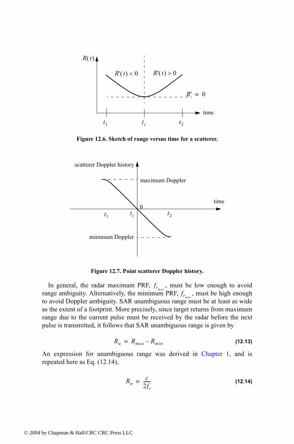
© 200
In general, the radar maximum PRF, , must be low enough to avoid range ambiguity. Alternatively, the minimum PRF, , must be high enough to avoid Doppler ambiguity. SAR unambiguous range must be at least as wide as the extent of a footprint. More precisely, since target returns from maximum range due to the current pulse must be received by the radar before the next pulse is transmitted, it follows that SAR unambiguous range is given by
(12.13)
An expression for unambiguous range was derived in Chapter 1, and is repeated here as Eq. (12.14),
(12.14)
R t( )
R' 0=
R' t( ) 0< R' t( ) 0>
timetct1 t2
Figure 12.6. Sketch of range versus time for a scatterer.
scatterer Doppler history
time0
maximum Doppler
minimum Doppler
Figure 12.7. Point scatterer Doppler history.
tct1 t2
frmaxfrmin
Ru Rmax Rmin=
Ruc
2fr------=
4 by Chapman & Hall/CRC CRC Press LLC
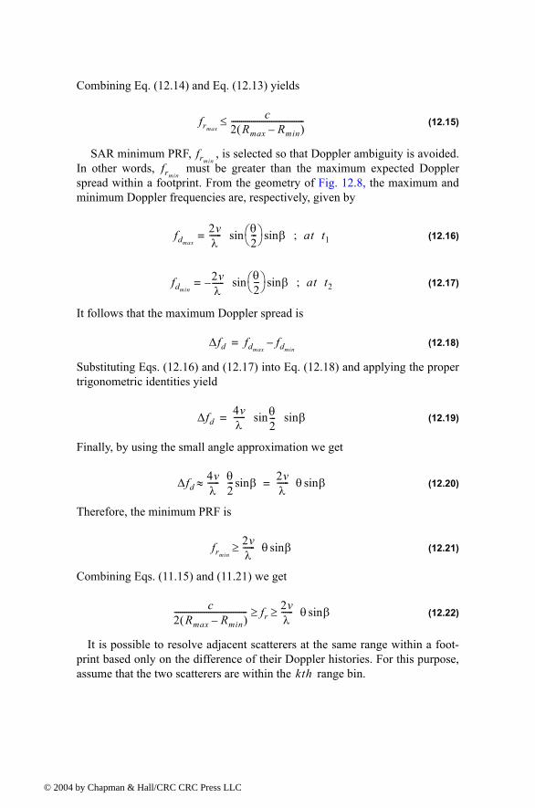
© 200
Combining Eq. (12.14) and Eq. (12.13) yields
(12.15)
SAR minimum PRF, , is selected so that Doppler ambiguity is avoided. In other words, must be greater than the maximum expected Doppler spread within a footprint. From the geometry of Fig. 12.8, the maximum and minimum Doppler frequencies are, respectively, given by
(12.16)
(12.17)
It follows that the maximum Doppler spread is
(12.18)
Substituting Eqs. (12.16) and (12.17) into Eq. (12.18) and applying the proper trigonometric identities yield
(12.19)
Finally, by using the small angle approximation we get
(12.20)
Therefore, the minimum PRF is
(12.21)
Combining Eqs. (11.15) and (11.21) we get
(12.22)
It is possible to resolve adjacent scatterers at the same range within a foot-print based only on the difference of their Doppler histories. For this purpose, assume that the two scatterers are within the range bin.
frmax
c2 Rmax Rmin( )------------------------------------≤
frminfrmin
fdmax
2vλ------ θ
2--- sin βsin= at t1;
fdmin
2vλ------
θ2--- sin βsin= at t2;
∆fd fdmaxfdmin
=
∆fd4vλ------ θ
2---sin βsin=
∆fd4vλ------ θ
2--- βsin≈ 2v
λ------ θ βsin=
frmin
2vλ------ θ βsin≥
c2 Rmax Rmin( )------------------------------------ fr
2vλ------ θ βsin≥ ≥
kth
4 by Chapman & Hall/CRC CRC Press LLC
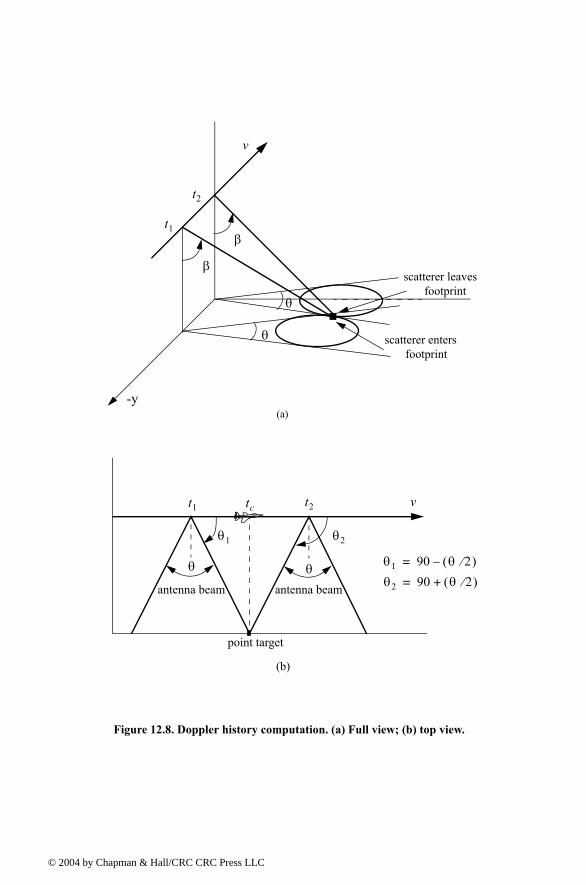
© 200
-y
β
v
β
t1
θ
θ
t2
scatterer entersfootprint
scatterer leavesfootprint
θ1
t1 t2tc
antenna beam antenna beam
θ θ
θ2
v
θ1 90 θ 2⁄( )=
θ2 90 θ 2⁄( )+=
point target
(a)
(b)
Figure 12.8. Doppler history computation. (a) Full view; (b) top view.
4 by Chapman & Hall/CRC CRC Press LLC
© 200
Denote their angular displacement as , and let be the minimum Doppler spread between the two scatterers such that they will appear in two distinct Doppler filters. Using the same methodology that led to Eq. (12.20) we get
(12.23)
where is the elevation angle corresponding to the range bin.
The bandwidth of the individual Doppler filters must be equal to the inverse of the coherent integration interval (i.e., ). It follows that
(12.24)
Substituting for yields
(12.25)
Therefore, the SAR azimuth resolution (within the range bin) is
(12.26)
Note that when , Eq. (12.26) is identical to Eq. (12.10).
12.4. SAR Radar EquationThe single pulse radar equation was derived in Chapter 1, and is repeated
here as Eq. (12.27),
(12.27)
where: is peak power; is antenna gain; is wavelength; is radar cross section; is radar slant range to the range bin; is Boltzmans constant;
is receiver noise temperature; is receiver bandwidth; and is radar losses. The radar cross section is a function of the radar resolution cell and ter-rain reflectivity. More precisely,
(12.28)
∆θ ∆fdmin
∆fdmin
2vλ------ ∆θ βksin=
βk kth
Tob ∆fdmin1 Tob⁄=
∆θ λ2vTob βksin----------------------------=
L vTob
∆θ λ2L βksin--------------------=
kth
∆Ag ∆θRk Rkλ
2L βksin--------------------= =
βk 90°=
SNRPtG
2λ2σ
4π( )3Rk4kT0BLLoss
---------------------------------------------=
Pt G λ σRk kth k
T0 B LLoss
σ σ0∆Rg= ∆Ag σ0∆Agcτ2----- ψgsec=
4 by Chapman & Hall/CRC CRC Press LLC
© 200
where is the clutter scattering coefficient, is the azimuth resolution, and Eq. (12.6) was used to replace the ground range resolution. The number of coherently integrated pulses within an observation interval is
(12.29)
where is the synthetic aperture size. Using Eq. (12.26) in Eq. (12.29) and rearranging terms yield
(12.30)
The radar average power over the observation interval is
(12.31)
The SNR for coherently integrated pulses is then
(12.32)
Substituting Eqs. (11.31), (11.30), and (11.28) into Eq. (12.32) and performing some algebraic manipulations give the SAR radar equation,
(12.33)
Eq. (12.33) leads to the conclusion that in SAR systems the SNR is (1) inversely proportional to the third power of range; (2) independent of azimuth resolution; (3) function of the ground range resolution; (4) inversely propor-tional to the velocity ; and (5) proportional to the third power of wavelength.
12.5. SAR Signal ProcessingThere are two signal processing techniques to sequentially produce a SAR
map or image; they are line-by-line processing and Doppler processing. The concept of SAR line-by-line processing is as follows: Through the radar linear motion a synthetic array is formed, where the elements of the current synthetic array correspond to the position of the antenna transmissions during the last observation interval. Azimuth resolution is obtained by forming narrow syn-thetic beams through combinations of the last observation interval returns. Fine range resolution is accomplished in real time by utilizing range gating and
σ0 ∆Ag
n frTobfrLv
-------==
L
nλRfr
2∆Agv---------------- βkcsc=
Pav Pt B⁄( )fr=
n
SNR( )n nSNR nPtG
2λ2σ
4π( )3Rk4kT0BLLoss
---------------------------------------------= =
SNR( )nPavG2λ3σ0
4π( )3Rk3kT0LLoss
-----------------------------------------∆Rg
2v---------- βkcsc=
v
4 by Chapman & Hall/CRC CRC Press LLC
© 200
pulse compression. For each range bin and each of the transmitted pulses dur-ing the last observation interval, the returns are recorded in a two-dimensional array of data that is updated for every pulse. Denote the two-dimensional array of data as .
To further illustrate the concept of line-by-line processing, consider the case where a map of size is to be produced, where is the number of azi-muth cells and is the number of range bins. Hence, is of size
, where the columns refer to range bins, and the rows refer to azimuth cells. For each transmitted pulse, the echoes from consecutive range bins are recorded sequentially in the first row of . Once the first row is com-pletely filled (i.e., returns from all range bins have been received), all data (in all rows) are shifted downward one row before the next pulse is transmitted. Thus, one row of is generated for every transmitted pulse. Consequently, for the current observation interval, returns from the first transmitted pulse will be located in the bottom row of , and returns from the last transmitted pulse will be in the first row of .
In SAR Doppler processing, the array is updated once every pulses so that a block of columns is generated simultaneously. In this case, refers to the number of transmissions during an observation interval (i.e., size of the synthetic array). From an antenna point of view, this is equivalent to having adjacent synthetic beams formed in parallel through electronic steer-ing.
12.6. Side Looking SAR Doppler ProcessingConsider the geometry shown in Fig. 12.9, and assume that the scatterer
is located within the range bin. The scatterer azimuth and elevation angles are and , respectively. The scatterer elevation angle is assumed to be equal to , the range bin elevation angle. This assumption is true if the ground range resolution, , is small; otherwise, for some small ; in this chapter .
The normalized transmitted signal can be represented by
(12.34)
where is the radar operating frequency, and denotes the transmitter phase. The returned radar signal from is then equal to
(12.35)
where is the round-trip delay to the scatterer, and includes scat-terer strength, range attenuation, and antenna gain. The round-trip delay is
MAP
Na Nr× NaNr MAP
Na Nr×
MAP
MAP
MAPMAP
MAP NN N
N
Cikth
µi βi βiβk
∆Rg βi βk εi+=εi εi 0=
s t( ) 2πf0t ξ0( )cos=
f0 ξ0Ci
si t µi,( ) Ai 2πf0 t τ i t µi,( )( ) ξ0[ ]cos=
τi t µi,( ) Ai
4 by Chapman & Hall/CRC CRC Press LLC
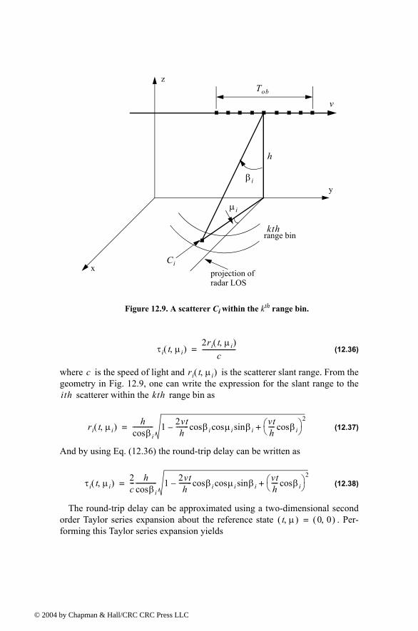
© 200
(12.36)
where is the speed of light and is the scatterer slant range. From the geometry in Fig. 12.9, one can write the expression for the slant range to the
scatterer within the range bin as
(12.37)
And by using Eq. (12.36) the round-trip delay can be written as
(12.38)
The round-trip delay can be approximated using a two-dimensional second order Taylor series expansion about the reference state . Per-forming this Taylor series expansion yields
Tob
Figure 12.9. A scatterer Ci within the kth range bin.
x
z
h
y
kth
µi
range bin
βi
v
Ciprojection of radar LOS
τi t µi,( )2ri t µi,( )
c---------------------=
c ri t µi,( )
ith kth
ri t µi,( ) hβicos
------------- 1 2vth
-------- βicos µicos βisinvth---- βicos
2+=
τi t µi,( ) 2c--- h
βicos------------- 1 2vt
h-------- βicos µicos βisin
vth---- βicos
2+=
t µ,( ) 0 0,( )=
4 by Chapman & Hall/CRC CRC Press LLC
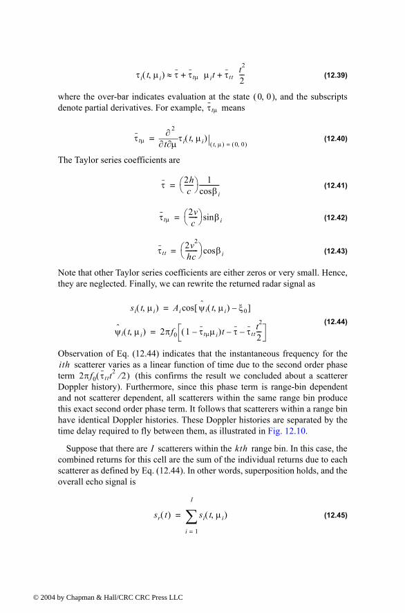
© 200
(12.39)
where the over-bar indicates evaluation at the state , and the subscripts denote partial derivatives. For example, means
(12.40)
The Taylor series coefficients are
(12.41)
(12.42)
(12.43)
Note that other Taylor series coefficients are either zeros or very small. Hence, they are neglected. Finally, we can rewrite the returned radar signal as
(12.44)
Observation of Eq. (12.44) indicates that the instantaneous frequency for the scatterer varies as a linear function of time due to the second order phase
term (this confirms the result we concluded about a scatterer Doppler history). Furthermore, since this phase term is range-bin dependent and not scatterer dependent, all scatterers within the same range bin produce this exact second order phase term. It follows that scatterers within a range bin have identical Doppler histories. These Doppler histories are separated by the time delay required to fly between them, as illustrated in Fig. 12.10.
Suppose that there are scatterers within the range bin. In this case, the combined returns for this cell are the sum of the individual returns due to each scatterer as defined by Eq. (12.44). In other words, superposition holds, and the overall echo signal is
(12.45)
τi t µi,( ) τ τtµ µit τt tt2
2---+ +≈
0 0,( )τtµ
τtµ t µ∂
2
∂∂ τi t µi,( )
t µ,( ) 0 0,( )==
τ 2hc
------ 1
βicos-------------=
τtµ2vc
------ βisin=
τtt2v2
hc-------- βicos=
si t µi,( ) Ai ψ i t µi,( ) ξ0[ ]cos=
ψ i t µi,( ) 2πf0 1 τtµµi( )t τ τt tt2
2---=
ith2πf0 τt tt
2 2⁄( )
I kth
sr t( ) si t µi,( )
i 1=
I
∑=
4 by Chapman & Hall/CRC CRC Press LLC
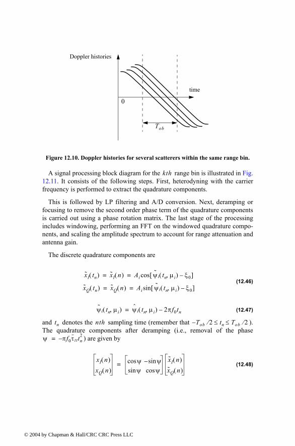
© 200
A signal processing block diagram for the range bin is illustrated in Fig. 12.11. It consists of the following steps. First, heterodyning with the carrier frequency is performed to extract the quadrature components.
This is followed by LP filtering and A/D conversion. Next, deramping or focusing to remove the second order phase term of the quadrature components is carried out using a phase rotation matrix. The last stage of the processing includes windowing, performing an FFT on the windowed quadrature compo-nents, and scaling the amplitude spectrum to account for range attenuation and antenna gain.
The discrete quadrature components are
(12.46)
(12.47)
and denotes the sampling time (remember that ). The quadrature components after deramping (i.e., removal of the phase
) are given by
(12.48)
Doppler histories
time
Figure 12.10. Doppler histories for several scatterers within the same range bin.
0
Tob
kth
x I tn( ) x I n( ) Ai ψ i tn µi,( ) ξ0[ ]cos= =
xQ tn( ) xQ n( ) Ai ψ i tn µi,( ) ξ0[ ]sin= =
ψ i tn µi,( ) ψ i tn µi,( ) 2πf0tn=
tn nth Tob 2⁄ tn Tob 2⁄≤ ≤
ψ πf0 τtttn2=
xI n( )
xQ n( )ψcos ψsin
ψsin ψcosx I n( )
xQ n( )=
4 by Chapman & Hall/CRC CRC Press LLC
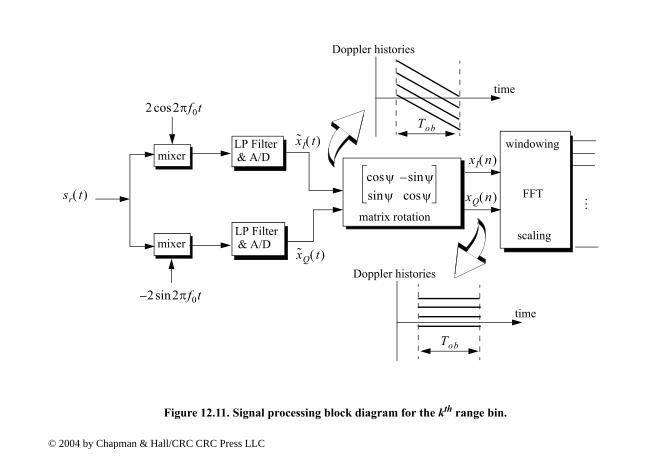
Side Looking SAR Doppler Processing
605
windowing
scaling
FFT
…
time
time
b
range bin.
xQ n( )
xI n( )
mixermixer
LP Filter
LP Filter
2 2πf0tcos
sr t( )
2 2πf0tsin
xQ t( )
x I t( ) & A/D
& A/D
ψcos ψsin
ψsin ψcosmatrix rotation
Doppler histories
Tob
Doppler histories
To
Figure 12.11. Signal processing block diagram for the kth
© 2004 by Chapman & Hall/CRC CRC Press LLC
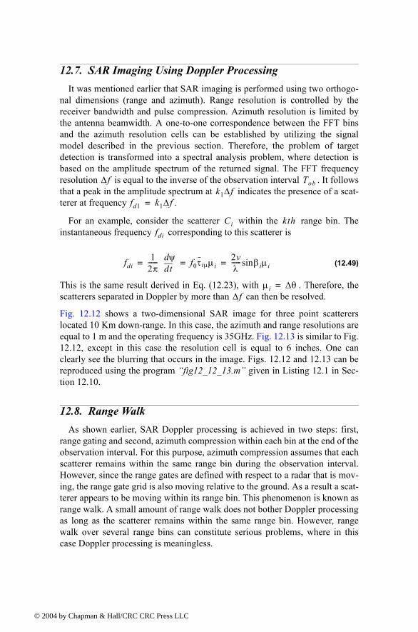
© 200
12.7. SAR Imaging Using Doppler ProcessingIt was mentioned earlier that SAR imaging is performed using two orthogo-
nal dimensions (range and azimuth). Range resolution is controlled by the receiver bandwidth and pulse compression. Azimuth resolution is limited by the antenna beamwidth. A one-to-one correspondence between the FFT bins and the azimuth resolution cells can be established by utilizing the signal model described in the previous section. Therefore, the problem of target detection is transformed into a spectral analysis problem, where detection is based on the amplitude spectrum of the returned signal. The FFT frequency resolution is equal to the inverse of the observation interval . It follows that a peak in the amplitude spectrum at indicates the presence of a scat-terer at frequency .
For an example, consider the scatterer within the range bin. The instantaneous frequency corresponding to this scatterer is
(12.49)
This is the same result derived in Eq. (12.23), with . Therefore, the scatterers separated in Doppler by more than can then be resolved.
Fig. 12.12 shows a two-dimensional SAR image for three point scatterers located 10 Km down-range. In this case, the azimuth and range resolutions are equal to 1 m and the operating frequency is 35GHz. Fig. 12.13 is similar to Fig. 12.12, except in this case the resolution cell is equal to 6 inches. One can clearly see the blurring that occurs in the image. Figs. 12.12 and 12.13 can be reproduced using the program fig12_12_13.m given in Listing 12.1 in Sec-tion 12.10.
12.8. Range WalkAs shown earlier, SAR Doppler processing is achieved in two steps: first,
range gating and second, azimuth compression within each bin at the end of the observation interval. For this purpose, azimuth compression assumes that each scatterer remains within the same range bin during the observation interval. However, since the range gates are defined with respect to a radar that is mov-ing, the range gate grid is also moving relative to the ground. As a result a scat-terer appears to be moving within its range bin. This phenomenon is known as range walk. A small amount of range walk does not bother Doppler processing as long as the scatterer remains within the same range bin. However, range walk over several range bins can constitute serious problems, where in this case Doppler processing is meaningless.
∆f Tobk1∆f
fd1 k1∆f=
Ci kthfdi
fdi1
2π------
tddψ f0τtµµi
2vλ------ βisin µi= = =
µi ∆θ=∆f
4 by Chapman & Hall/CRC CRC Press LLC
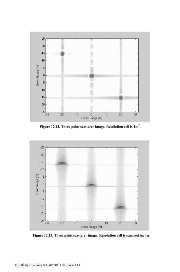
© 200
Figure 12.12. Three point scatterer image. Resolution cell is 1m2.
Figure 12.13. Three point scatterer image. Resolution cell is squared inches.
4 by Chapman & Hall/CRC CRC Press LLC
© 200
12.9. A Three-Dimensional SAR Imaging TechniqueThis section presents a new three-dimensional (3-D) Synthetic Aperture
Radar (SAR) imaging technique.1 It utilizes a linear array in transverse motion to synthesize a two-dimensional (2-D) synthetic array. Elements of the linear array are fired sequentially (one element at a time), while all elements receive in parallel. A 2-D information sequence is computed from the equiphase two-way signal returns. A signal model based on a third-order Taylor series expan-sion about incremental relative time, azimuth, elevation, and target height is used. Scatterers are detected as peaks in the amplitude spectrum of the infor-mation sequence. Detection is performed in two stages. First, all scatterers within a footprint are detected using an incomplete signal model where target height is set to zero. Then, processing using the complete signal model is per-formed only on range bins containing significant scatterer returns. The differ-ence between the two images is used to measure target height. Computer simulation shows that this technique is accurate and virtually impulse invari-ant.
12.9.1. Background
Standard Synthetic Aperture Radar (SAR) imaging systems are generally used to generate high resolution two-dimensional (2-D) images of ground ter-rain. Range gating determines resolution along the first dimension. Pulse com-pression techniques are usually used to achieve fine range resolution. Such techniques require the use of wide band receiver and display devices in order to resolve the time structure in the returned signals. The width of azimuth cells provides resolution along the other dimension. Azimuth resolution is limited by the duration of the observation interval.
This section presents a three-dimensional (3-D) SAR imaging technique based on Discrete Fourier Transform (DFT) processing of equiphase data col-lected in sequential mode (DFTSQM). It uses a linear array in transverse motion to synthesize a 2-D synthetic array. A 2-D information sequence is computed from the equiphase two-way signal returns. To this end, a new signal model based on a third-order Taylor series expansion about incremental rela-tive time, azimuth, elevation, and target height is introduced. Standard SAR imaging can be achieved using an incomplete signal model where target height is set to zero. Detection is performed in two stages. First, all scatterers within a footprint are detected using an incomplete signal model, where target height is set to zero. Then, processing using the complete signal model is performed
1. This section is extracted from: Mahafza, B. R. and Sajjadi, M., Three-Dimensional SAR Imaging Using a Linear Array in Transverse Motion, IEEE - AES Trans., Vol. 32, No. 1, January 1996, pp. 499-510.
4 by Chapman & Hall/CRC CRC Press LLC
© 200
only on range bins containing significant scatterer returns. The difference between the two images is used as an indication of target height. Computer simulation shows that this technique is accurate and virtually impulse invari-ant.
12.9.2. DFTSQM Operation and Signal ProcessingLinear Arrays
Consider a linear array of size , uniform element spacing , and wave-length . Assume a far field scatterer located at direction-sine . DFTSQM operation for this array can be described as follows. The elements are fired sequentially, one at a time, while all elements receive in parallel. The echoes are collected and integrated coherently on the basis of equal phase to compute a complex information sequence . The x-coordinates, in -units, of the element with respect to the center of the array is
(12.50)
The electric field received by the element due to the firing of the , and reflection by the far field scatterer , is
(12.51)
(12.52)
(12.53)
where is the target cross section, is the two-way element gain, and is the range attenuation with respect to reference range . The scat-
terer phase is assumed to be zero; however it could be easily included. Assum-ing multiple scatterers in the arrays FOV, the cumulative electric field in the path due to reflections from all scatterers is
(12.54)
where the subscripts denote the quadrature components. Note that the variable part of the phase given in Eq. (12.52) is proportional to the integers resulting from the sums . In the far field operation there are a total of distinct sums. Therefore, the electric fields with paths of the same sums can be collected
N dλ P βlsin
b m( ) m; 0 2N 1,= d xn
th
xnN 1
2------------- n+
n; 0 …N 1,= =
x2th x1
th
lth P
E x1 x2 sl;,( ) G2 sl( )R0
R-----
4σl exp jφ x1 x2 sl;,( )( )=
φ x1 x2, sl;( ) 2πλ
------ x1 x2+( ) sl( )=
sl βlsin=
σl G2 sl( )R0 R⁄( )4 R0
x1 x2⇒
E x1 x2,( ) EI x1 x2 sl;,( ) jEQ x1 x2 sl;,( )+[ ]all l∑=
I Q,( )
xn1 xn2+( ); n1 n2,( ) 0 …N 1,= 2N 1( ) xn1 xn2+( )
xn1 xn2+( )
4 by Chapman & Hall/CRC CRC Press LLC
© 200
coherently. In this manner the information sequence is computed, where is set to zero. At the same time one forms the sequence which keeps track of the number of returns that have the same sum. More precisely, for
(12.55)
(12.56)
It follows that
(12.57)
which is a triangular shape sequence.
The processing of the sequence is performed as follows: (1) the weighting takes the sequence into account; (2) the complex sequence
is extended to size , a power integer of two, by zero padding; (3) the DFT of the extended sequence is computed,
(12.58)
and, (4) after compensation for antenna gain and range attenuation, scatterers are detected as peaks in the amplitude spectrum . Note that step (4) is true only when
(12.59)
where denotes the direction-sine of the scatterer, and is implied in Eq. (12.59).
The classical approach to multiple target detection is to use a phased array antenna with phase shifting and tapering hardware. The array beamwidth is proportional to , and the first sidelobe is at about -13 dB. On the other hand, multiple target detection using DFTSQM provides a beamwidth propor-tional to as indicated by (Eq. (12.59), which has the effect of dou-bling the arrays resolution. The first sidelobe is at about -27 dB due to the triangular sequence . Additionally, no phase shifting hardware is required for detection of targets within a single elements field of view.
b m( ) m; 0 2N 1,= b 2N 1( )
c m( ) m; 0 …2N 2,= xn1 xn2+( )
m n1 n2+= ; n1 n2,( ) …0 N 1,=
b m( ) b m( ) E xn1 xn2,( )+=
c m( ) c m( ) 1+=
c m( ) m; 0 …2N 2,= m 1 m;+ 0 …N 2,=
N m; N 1=
2N 1 m m N …2N 2,=
=
b m( ) c m( )
b m( ) NFb' m( ) m; 0 NF 1,=
B q( ) b' m( ) exp j2πqmNF
-------------- q;⋅
m 0=
NF 1
∑ 0 …NF 1,= =
B q( )
βqsin λq2Nd---------- q; 0 …2N 1,= =
βqsin qth NF 2N=
λ Nd⁄( )
λ 2Nd⁄( )
c m( )
4 by Chapman & Hall/CRC CRC Press LLC
© 200
Rectangular Arrays DFTSQM operation and signal processing for 2-D arrays can be described as
follows. Consider an rectangular array. All elements are fired sequentially, one at a time. After each firing, all the array elements receive in parallel. Thus, samples of the quadrature components are col-lected after each firing, and a total of samples will be collected. How-ever, in the far field operation, there are only distinct equiphase returns. Therefore, the collected data can be added coherently to form a 2-D information array of size . The two-way radiation pattern is computed as the modulus of the 2-D amplitude spectrum of the information array. The processing includes 2-D windowing, 2-D Discrete Fourier Transformation, antenna gain, and range attenuation compensation. The field of view of the 2-D array is determined by the 3 dB pattern of a single element. All the scatterers within this field will be detected simultaneously as peaks in the amplitude spectrum.
Consider a rectangular array of size , with uniform element spacing , and wavelength . The coordinates of the element, in -
units, are
(12.60)
(12.61)
Assume a far field point defined by the azimuth and elevation angles . In this case, the one-way geometric phase for an element is
(12.62)
Therefore, the two-way geometric phase between the and ele-ments is
(12.63)
The two-way electric field for the scatterer at is
(12.64)
Assuming multiple scatterers within the arrays FOV, then the cumulative elec-tric field for the two-way path is given by
Nx Ny× NxNyNxNy
NxNyNxNy( )2
2Nx 1( ) 2Ny 1( )×
2Nx 1( ) 2Ny 1( )×
N N×dx dy d= = λ nth d
xnN 1
2------------- n+
n; 0 …N 1,= =
ynN 1
2------------- n+
n; 0 …N 1,= =
Pα β,( )
ϕ' x y,( ) 2πλ
------ x β αcossin y β αsinsin+[ ]=
x1 y1,( ) x2 y2,( )
ϕ x1 y1 x2 y2, , ,( ) 2πλ
------ βsin x1 x2+( ) αcos y1 y2+( ) αsin+[ ]=
lth αl βl,( )
E x1 x2 y1 y2 αl βl,;, , ,( ) G2 βl( )R0
R-----
4σl exp j ϕ x1 y1 x2 y2, , ,( )( )[ ]=
x1 y1,( ) x2 y2,( )⇒
4 by Chapman & Hall/CRC CRC Press LLC
© 200
(12.65)
All formulas for the 2-D case reduce to those of a linear array case by setting and .
The variable part of the phase given in Eq. (12.63) is proportional to the inte-gers and . Therefore, after completion of the sequential fir-ing, electric fields with paths of the same sums, where
(12.66)
(12.67)
can be collected coherently. In this manner the 2-D information array is computed. The coefficient sequence is also computed. More precisely,
(12.68)
(12.69)
It follows that
(12.70)
The processing of the complex 2-D information array is simi-lar to that of the linear case with the exception that one should use a 2-D DFT. After antenna gain and range attenuation compensation, scatterers are detected as peaks in the 2-D amplitude spectrum of the information array. A scatterer located at angles will produce a peak in the amplitude spectrum at DFT indexes , where
(12.71)
(12.72)
Derivation of Eq. (12.71) is in Section 12.9.7.
12.9.3. Geometry for DFTSQM SAR Imaging
Fig. 12.14 shows the geometry of the DFTSQM SAR imaging system. In this case, denotes the central time of the observation interval, . The air-craft maintains both constant velocity and height . The origin for the rela-
E x1 x2 y1 y2, , ,( ) E x1 x2 y1 y2 αl βl,;, , ,( )all scatterers∑=
Ny 1= α 0=
x1 x2+( ) y1 y2+( )i j,( )
i xn1 xn2 i;+ N 1( ) … N 1( ),= =
j yn1 yn2 j;+ N 1( ) … N 1( ),= =
b mx my,( ) mx my,( ); 0 …2N 1,= c mx my,( ) mx my,( ); 0 …2N 2,=
for mx n1 n2 and my n1 n2+=+=n1 0 …N 1,= and n2, 0 …N 1,=
b mx my,( ) b mx my,( ) E xn1 yn1 xn2 yn2, , ,( )+=
c mx my,( ) Nx mx Nx 1( )( ) Ny my Ny 1( )( )×=
b mx my,( )
αl βl,( )pl ql,( )
αlql
pl---- atan=
βlsinλpl
2Nd αlcos-------------------------
λql
2Nd αlsin------------------------= =
tc Dobv h
4 by Chapman & Hall/CRC CRC Press LLC
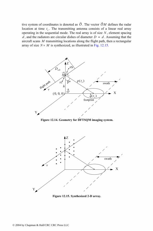
© 200
tive system of coordinates is denoted as . The vector defines the radar location at time . The transmitting antenna consists of a linear real array operating in the sequential mode. The real array is of size , element spacing
, and the radiators are circular dishes of diameter . Assuming that the aircraft scans transmitting locations along the flight path, then a rectangular array of size is synthesized, as illustrated in Fig. 12.15.
O OMtc
Nd D d=
MN M×
X
Z
Y
vflight path
0 0 0, ,( ) O
β∗
q tc( )
ρ tc( )
Dob
M tc
hswath
footprint
#1
#N
Figure 12.14. Geometry for DFTSQM imaging system.
X
Z
Y
v
swath
Figure 12.15. Synthesized 2-D array.
4 by Chapman & Hall/CRC CRC Press LLC
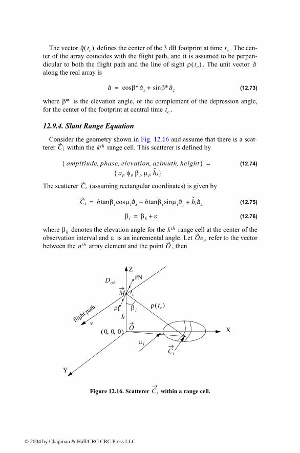
© 200
The vector defines the center of the 3 dB footprint at time . The cen-ter of the array coincides with the flight path, and it is assumed to be perpen-dicular to both the flight path and the line of sight . The unit vector along the real array is
(12.73)
where is the elevation angle, or the complement of the depression angle, for the center of the footprint at central time .
12.9.4. Slant Range Equation
Consider the geometry shown in Fig. 12.16 and assume that there is a scat-terer within the range cell. This scatterer is defined by
(12.74)
The scatterer (assuming rectangular coordinates) is given by
(12.75)
(12.76)
where denotes the elevation angle for the range cell at the center of the observation interval and is an incremental angle. Let refer to the vector between the array element and the point , then
q tc( ) tc
ρ tc( ) a
a β∗axcos β∗azsin+=
β∗tc
Ci kth
ampltiude phase elevation azimuth height, , , , ai φi βi µi h i, , , ,
=
Ci
Ci h βitan µicos ax h βitan µisin ay h iaz+ +=
βi βk ε+=
βk kth
ε Oennth O
X
Z
Y
vflight path
0 0 0, ,( ) O
βiρ tc( )
Dob
M tc
h#1
#N
Figure 12.16. Scatterer within a range cell.Ci
Ci
µi
4 by Chapman & Hall/CRC CRC Press LLC
© 200
(12.77)
(12.78)
The range between a scatterer within the range cell and the element of the real array is
(12.79)
It is more practical to use the scatterer's elevation and azimuth direction-sines rather than the corresponding increments. Therefore, define the scat-terer's azimuth and elevation direction-sines as
(12.80)
(12.81)
Then, one can rewrite Eq. (12.79) as
(12.82)
(12.83)
Expanding as a third order Taylor series expansion about incremental yields
(12.84)
where subscripts denote partial derivations, and the over-bar indicates evalua-tion at the state . Note that
(12.85)
Section 12.9.8 has detailed expressions of all non-zero Taylor series coeffi-cients for the range cell.
Even at the maximum increments , the terms:
Oen Dn β∗cos ax vtay Dn β∗sin h+( )az+ +=
Dn1 N
2------------- n+ d n; 0 …N 1,= =
C kth nth
rn2 t ε µ h D; n, , ,( ) Dn
2 v2t2 h h( )2 2Dn β∗sin h h( )h βk ε+( ) h βk ε+( )tan 2Dn β∗cos µcos 2vt µsin[ ]tan
+ + + +=
s µsin=
u εsin=
rn2 t s u h Dn;, , ,( ) Dn
2 v2t2 h h( )2 h2f2 u( )2Dn β∗sin h h( ) 2Dnh β∗cos f u( ) 1 s2 2vhtf u( )s( )
+ + + +=
f u( ) βk uasin+( )tan=
rnt s u h, , ,( )
r t s u h Dn;, , ,( ) r rh h ruu rh h
h 2
2----- rh uh u rss
s2
2---- rstst
rttt2
2---- ruu
u2
2----- rh h h
h 3
6----- rh h u
h 2u2
-------- rh sth st rh uu
h u2
2--------
rh ssh s2
2-------- russ
us2
2-------- rstustu rsuu
su2
2-------- rth h
th 2
2------- rutt
ut2
2------- ruuu
u3
6-----
+ + + + + + +
+ + + + + +
+ + + + + +
=
t s u h, , ,( ) 0 0 0 0, , ,( )=
rs rt rh s rh t rsu rtu rh h s rh h t rh su rh tu
rsss rsst rstt rttt rtsu 0= = = = = = = = = =
= = = = =
kth
tmx smx umx h mx, , ,
4 by Chapman & Hall/CRC CRC Press LLC
© 200
(12.86)
are small and can be neglected. Thus, the range is approximated by
(12.87)
Consider the following two-way path: the element transmitting, scatterer reflecting, and the element receiving. It follows that the round trip
delay corresponding to this two-way path is
(12.88)
where is the speed of light.
12.9.5. Signal Synthesis
The observation interval is divided into subintervals of width . During each subinterval, the real array is operated in
sequential mode, and an array length of is synthesized. The number of sub-intervals is computed such that is large enough to allow sequential transmission for the real array without causing range ambiguities. In other words, if the maximum range is denoted as then
(12.89)
Each subinterval is then partitioned into sampling subintervals of width. The location represents the sampling time at which the ele-
ment is transmitting during the subinterval.
The normalized transmitted signal during the subinterval for the element is defined as
(12.90)
where denotes the transmitter phase, and is the system operating fre-quency. Assume that there is only one scatterer, , within the range cell
rh h hh 3
6----- rh h u
h 2u2
-------- rh uuh u2
2-------- rh ss
h s2
2--------
russus2
2-------- rstustu rsuu
su2
2-------- rth h
th 2
2------- rutt
ut2
2------- ruuu
u3
6-----, , , , ,
, , , ,
rn
r t s u h Dn;, , ,( ) r rh h ruu rh h
h 2
2----- rh uh u
rsss2
2---- rstst rtt
t2
2---- ruu
u2
2----- rh sth
st
+ + + + +
+ + + +
=
n1th
Ci n2th
τn1n2
1c--- rn1
t s u h Dn1;, , ,( ) rn2
t s u h Dn2;, , ,( )+( )=
c
M∆t Dob M÷( )=
2NM ∆t
Rmx
∆t N2Rmx
c------------>
N2Rmx c⁄ tmn nth
mth
mth nth
sn tmn( ) 2πfotmn ζ+( )cos=
ζ foCi kth
4 by Chapman & Hall/CRC CRC Press LLC
© 200
defined by . The returned signal at the element due to fir-ing from the element and reflection from the scatterer is
(12.91)
where represents the two-way antenna gain, and the term denotes the range attenuation at the range cell. The analysis in this paper will assume hereon that and are both equal to zeroes.
Suppose that there are scatterers within the range cell, with angular locations given by
(12.92)
The composite returned signal at time within this range cell due to the path is
(12.93)
The platform motion synthesizes a rectangular array of size , where only one column of elements exists at a time. However, if and the real array is operated in the sequential mode, a square planar array of size
is synthesized. The element spacing along the flight path is .
Consider the range bin. The corresponding two-dimensional information sequence consists of similar vectors. The vector represents the returns due to the sequential firing of all ele-ments during the subinterval. Each vector has rows, and it is extended, by adding zeroes, to the next power of two. For example, consider the subinterval, and let . Then, the elements of the extended column are
(12.94)
ai φi si ui h i, , , ,( ) n2th
n1th Ci
si n1 n2 tmn1;,( ) aiG2 βisin( ) ρk tc( ) ρ tc( )⁄( )4
2πfo tmn1τn1n2
( ) ζ φi+[ ]cos=
G2 ρk tc( ) ρ tc( )⁄( )4
kth
ζ φi
No kth
ai φi s, i ui h i, , ,( ) i; 1 …No,=
tmn1n1 all Ci n2⇒ ⇒( )
s n1 n2 tmn1;,( ) si n1 n2 tmn1
;,( )
i 1=
No
∑=
N M×N M 2N=
2N 2N×dy vDob M⁄=
kth
bk n m,( ) n m,( ); 0 …2N 2,= 2Nmth N
mth 2N 1( )
mth M 2N 4= =bk n m,( )
bk 0 m,( ) bk 1 m,( ) bk 2 m,( ) bk 3 m,( ) bk 4 m,( ) bk 5 m,( )bk 6 m,( ) bk 7 m,( ),
,,,,,, s 0 0 tmn0
;,( ) s 0 1 tmn0;,( ) s 1 0 tmn1
;,( )+s 0 2 tmn0
;,( ) s 1 1 tmn1;,( ) s 2 0 tmn2
;,( ) s 0 3 tmn0;,( ) s 1 2 tmn1
;,( )s 2 1 tmn2
;,( ) s 3 0 tmn3;,( ) s 1 3 tmn1
;,( ) s 2 2 tmn2;,( )
s 3 1 tmn3;,( ) s 2 3 tmn2
;,( ) s 3 2 tmn3;,( ) s 3 3 tmn3
;,( ) 0, ,+ ,+ +,
+ ++
,+ +, ,=
4 by Chapman & Hall/CRC CRC Press LLC
© 200
12.9.6. Electronic Processing
Consider again the range cell during the subinterval, and the two-way path: element transmitting and element receiving. The analog quadrature components corresponding to this two-way path are
(12.95)
(12.96)
(12.97)
where denotes antenna gain, range attenuation, and scatterers' strengths. The subscripts for have been dropped for notation simplicity. Rearranging Eq. (12.97) and collecting terms yields
(12.98)
After analog to digital (A/D) conversion, deramping of the quadrature compo-nents to cancel the quadratic phase is performed. Then, the digital quadrature components are
(12.99)
(12.100)
kth mth
n1th n2
th
sI⊥ n1 n2 t;,( ) B ψ⊥cos=
sQ⊥ n1 n2 t;,( ) B ψ⊥sin=
ψ⊥ 2πf0 t 1c--- 2r rh Dn1
( ) rh Dn2( )+( )h ru Dn1
( ) ru Dn2( )+( )u
rh h Dn1( ) rh h Dn2
( )+( )h 2
2----- rh u Dn1
( ) rh u Dn2( )+( )h u
rss Dn1( ) rss Dn2
( )+( )s2
2---- 2rstst 2rtt
t2
2----
ruu Dn1( ) ruu Dn2
( )+( )u2
2----- rh st Dn1
( ) rh st Dn2( )+( )h st ]
+ + +
+
+ + +
+ +
=
Bt
ψ⊥2πf0
c----------- tc 2rsts rh st Dn1
( ) rh st Dn2( )+( )h s+[ ]t rttt2
2r rh Dn1( ) rh Dn2
( )+( )h ru Dn1( ) ru Dn2
( )+( )u
ruu Dn1( ) ruu Dn2
( )+( )u2
2----- rh h Dn1
( ) rh h Dn2( )+( )h
2
2-----
rh u Dn1( ) rh u Dn2
( )+( )h u rss Dn1( ) rss Dn2
( )+( )s2
2----
+
+
+ + +
+
=
2 πf0rttt2 c⁄( )
sI n1 n2 t;,( ) B ψcos=
sQ n1 n2 t;,( ) B ψsin=
4 by Chapman & Hall/CRC CRC Press LLC
© 200
(12.101)
The instantaneous frequency for the scatterer within the range cell is computed as
(12.102)
Substituting the actual values for , , and collecting terms yields
(12.103)
Note that if , then
(12.104)
which is the Doppler value corresponding to a ground patch (see Eq. (12.49)).
The last stage of the processing consists of three steps: (1) two-dimensional windowing; (2) performing a two-dimensional DFT on the windowed quadra-ture components; and (3) scaling to compensate for antenna gain and range attenuation.
12.9.7. Derivation of Eq. (12.71)
Consider a rectangular array of size , with uniform element spacing , and wavelength . Assume sequential mode operation where
elements are fired sequentially, one at a time, while all elements receive in par-allel. Assume far field observation defined by azimuth and elevation angles
. The unit vector on the line of sight, with respect to , is given by
(12.105)
The element of the array can be defined by the vector
(12.106)
where . The one-way geometric phase for this element is
(12.107)
ψ ψ⊥ 2πf0t 2πf0rttt2
c----+=
ith kth
fdi1
2π------
tddψ f0
c--- 2rsts rh st Dn1
( ) rh st Dn2( )+( )h s ]+[= =
rst rh st Dn1( ) rh st Dn2
( )
fdi2v βksin
λ-------------------
h sρk
2 tc( )-------------- h Dn1
Dn2+( ) β∗sin+( ) s
=
h 0=
fdi2vλ------ βksin µsin=
N N×dx dy d= = λ
α β,( ) u O
u β α axcossin β α aysinsin β azcos+ +=
nx ny,( )th
e nx ny,( ) nxN 1
2-------------
d ax nyN 1
2-------------
d ay+=
nx ny, 0 …N 1,=( )
ϕ' nx ny,( ) k u e nx ny,( )•( )=
4 by Chapman & Hall/CRC CRC Press LLC
© 200
where is the wave-number, and the operator indicates dot product. Therefore, the two-way geometric phase between the and
elements is
(12.108)
The cumulative two-way normalized electric field due to all transmissions is
(12.109)
where the subscripts and , respectively, refer to the transmitted and received electric fields. More precisely,
(12.110)
(12.111)
In this case, denotes the tapering sequence. Substituting Eqs. (12.108), (12.110), and (12.111) into Eq. (12.109) and grouping all fields with the same two-way geometric phase yields
(12.112)
(12.113)
(12.114)
(12.115)
(12.116)
The two-way array pattern is then computed as
(12.117)
Consider the two-dimensional DFT transform, , of the array
k 2π λ⁄= •( )nx1 ny1,( )
nx2 ny2,( )
ϕ nx1 ny1 nx2 ny2, , ,( ) k u e nx1 ny1,( ) e nx2 ny2,( )+ •[ ]=
E u( ) Et u( )Er u( )=
t r
Et u( ) w nxt nyt,( )exp jk u e nxt nyt,( )• [ ]
nyt 0=
N 1
∑nxt 0=
N 1
∑=
Er u( ) w nxr nyr,( )exp jk u e nxr nyr,( )• [ ]
nyr 0=
N 1
∑nxr 0=
N 1
∑=
w nx ny,( )
E u( ) ejδ w' m n,( )exp jkd βsin m αcos n αsin+( )[ ]
n 0=
Na 1
∑m 0=
Na 1
∑=
Na 2N 1=
m nxt nxr m;+ 0 …2N 2,= =
n nyt nyr n;+ 0 …2N 2,= =
δ d βsin2
----------------- N 1( ) αcos αsin+( )=
E u( ) w' m n,( )exp jkd βsin m αcos n αsin+( )[ ]
n 0=
Na 1
∑m 0=
Na 1
∑=
W' p q,( )w' nx ny,( )
4 by Chapman & Hall/CRC CRC Press LLC
© 200
(12.118)
Comparison of Eqs. (12.117) and Eq. (12.118) indicates that is equal to if
(12.119)
(12.120)
It follows that
(12.121)
12.9.8. Non-Zero Taylor Series Coefficients for the kth Range Cell
(12.122)
(12.123)
(12.124)
(12.125)
(12.126)
(12.127)
(12.128)
(12.129)
W' p q,( )
w' m n,( )exp j2πNa------ pm qn+( )
p q,;
n 0=
Na 1
∑m 0=
Na 1
∑ 0 …Na 1,
=
=
E u( )W' p q,( )
2πNa------ p
2πλ
------d β αcossin=
2πNa------ q
2πλ
------d β αsinsin=
α qp--- tan 1=
r Dn2 h2 1 βktan+( ) 2hDn β∗sin 2hDn β∗cos βktan+ + ρk tc( )= =
rh1r
------ h Dn β∗sin+( )=
ruh
r βkcos2------------------- h βktan Dn β∗cos( )=
rh h1r--- 1
r3---- h Dn β∗sin+( )=
rh u1r3---- h
βkcos2---------------- h Dn β∗tan+( ) h βktan Dn β∗cos( )=
rss1
4r3-------- 1
r--- h βktan Dn β∗cos( )+=
rst1r
------ hv βktan=
rttv2
r-----=
4 by Chapman & Hall/CRC CRC Press LLC
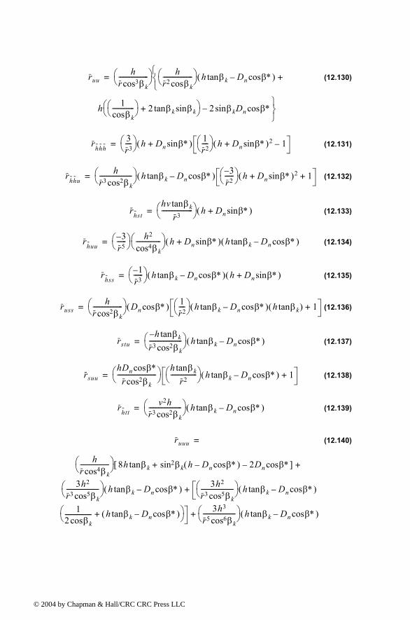
© 200
(12.130)
(12.131)
(12.132)
(12.133)
(12.134)
(12.135)
(12.136)
(12.137)
(12.138)
(12.139)
(12.140)
ruuh
r βkcos3------------------- h
r2 βkcos------------------- h βktan Dn β∗cos( )
h 1βkcos
-------------- 2 βktan βksin+ 2 βksin Dn β∗cos
+
=
rh h h3r3---- h Dn β∗sin+( ) 1
r2---- h Dn β∗sin+( )2 1=
rh h uh
r3 βkcos2--------------------- h βktan Dn β∗cos( ) 3
r2------ h Dn β∗sin+( )2 1+=
rh st
hv βktanr3
-------------------- h Dn β∗sin+( )=
rh uu3
r5------ h2
βkcos4---------------- h Dn β∗sin+( ) h βktan Dn β∗cos( )=
rh ss1
r3------ h βktan Dn β∗cos( ) h Dn β∗sin+( )=
russh
r βkcos2------------------- Dn β∗cos( ) 1
r2---- h βktan Dn β∗cos( ) h βktan( ) 1+=
rstuh βktan
r3 βkcos2--------------------- h βktan Dn β∗cos( )=
rsuuhDn β∗cos
r βkcos2------------------------- h βktan
r2----------------- h βktan Dn β∗cos( ) 1+=
rh ttv2h
r3 βkcos2--------------------- h βktan Dn β∗cos( )=
ruuu
hr βkcos4------------------- 8h βktan βksin2 h Dn β∗cos( ) 2Dn β∗cos+[ ]
3h2
r3 βkcos5--------------------- h βktan Dn β∗cos( ) 3h2
r3 βkcos5--------------------- h βktan Dn β∗cos( )
12 βkcos----------------- h βktan Dn β∗cos( )+ 3h3
r5 βkcos6--------------------- h βktan Dn β∗cos( )
+
+
+
=
4 by Chapman & Hall/CRC CRC Press LLC
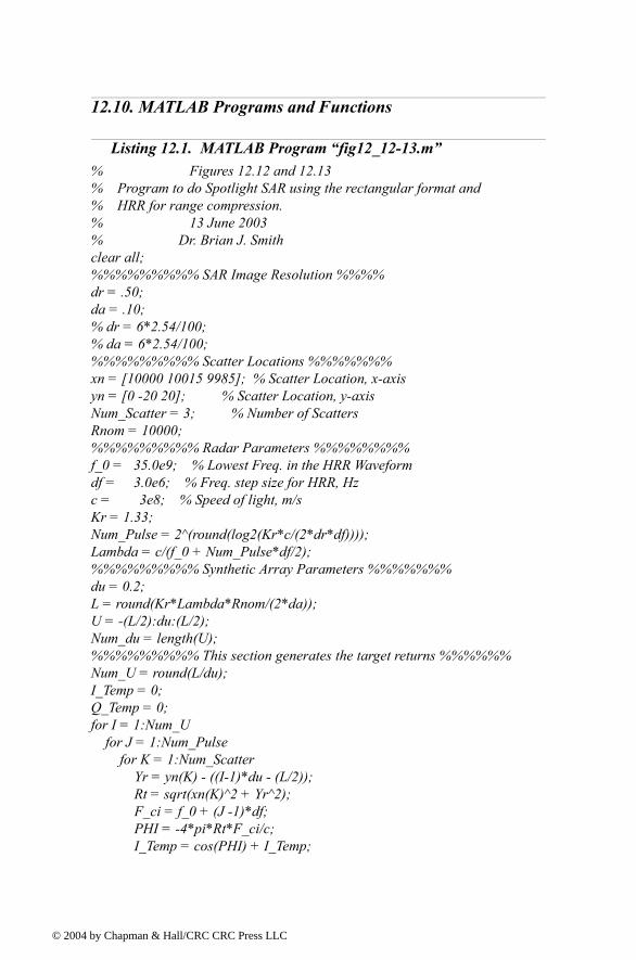
© 200
12.10. MATLAB Programs and Functions
Listing 12.1. MATLAB Program fig12_12-13.m% Figures 12.12 and 12.13% Program to do Spotlight SAR using the rectangular format and% HRR for range compression. % 13 June 2003% Dr. Brian J. Smithclear all;%%%%%%%%% SAR Image Resolution %%%%dr = .50;da = .10;% dr = 6*2.54/100;% da = 6*2.54/100;%%%%%%%%% Scatter Locations %%%%%%%xn = [10000 10015 9985]; % Scatter Location, x-axisyn = [0 -20 20]; % Scatter Location, y-axisNum_Scatter = 3; % Number of ScattersRnom = 10000;%%%%%%%%% Radar Parameters %%%%%%%%f_0 = 35.0e9; % Lowest Freq. in the HRR Waveformdf = 3.0e6; % Freq. step size for HRR, Hzc = 3e8; % Speed of light, m/sKr = 1.33;Num_Pulse = 2^(round(log2(Kr*c/(2*dr*df))));Lambda = c/(f_0 + Num_Pulse*df/2);%%%%%%%%% Synthetic Array Parameters %%%%%%%du = 0.2;L = round(Kr*Lambda*Rnom/(2*da));U = -(L/2):du:(L/2);Num_du = length(U);%%%%%%%%% This section generates the target returns %%%%%%Num_U = round(L/du);I_Temp = 0;Q_Temp = 0;for I = 1:Num_U for J = 1:Num_Pulse for K = 1:Num_Scatter Yr = yn(K) - ((I-1)*du - (L/2)); Rt = sqrt(xn(K)^2 + Yr^2); F_ci = f_0 + (J -1)*df; PHI = -4*pi*Rt*F_ci/c; I_Temp = cos(PHI) + I_Temp;
4 by Chapman & Hall/CRC CRC Press LLC
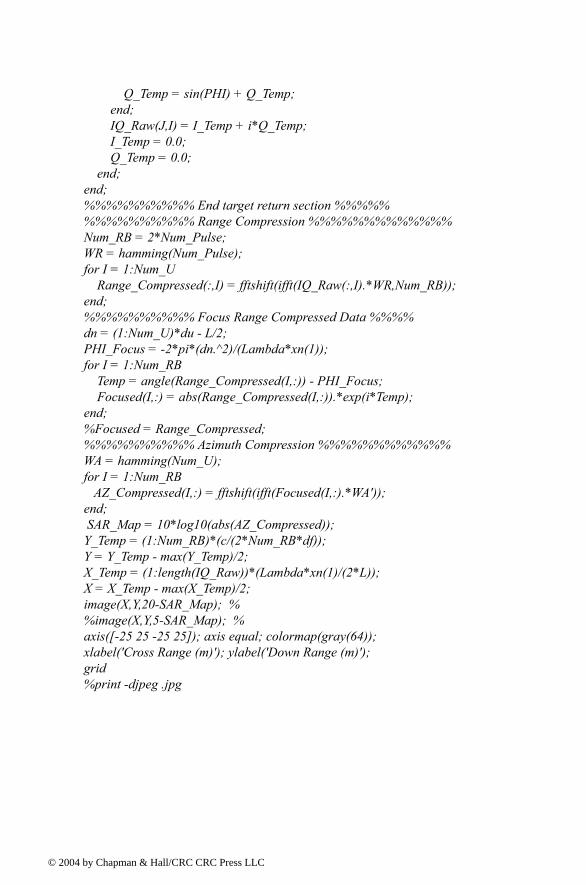
© 200
Q_Temp = sin(PHI) + Q_Temp; end; IQ_Raw(J,I) = I_Temp + i*Q_Temp; I_Temp = 0.0; Q_Temp = 0.0; end;end;%%%%%%%%%% End target return section %%%%%%%%%%%%%%% Range Compression %%%%%%%%%%%%%Num_RB = 2*Num_Pulse;WR = hamming(Num_Pulse);for I = 1:Num_U Range_Compressed(:,I) = fftshift(ifft(IQ_Raw(:,I).*WR,Num_RB));end;%%%%%%%%%% Focus Range Compressed Data %%%%dn = (1:Num_U)*du - L/2;PHI_Focus = -2*pi*(dn.^2)/(Lambda*xn(1));for I = 1:Num_RB Temp = angle(Range_Compressed(I,:)) - PHI_Focus; Focused(I,:) = abs(Range_Compressed(I,:)).*exp(i*Temp);end;%Focused = Range_Compressed;%%%%%%%%%% Azimuth Compression %%%%%%%%%%%%WA = hamming(Num_U);for I = 1:Num_RB AZ_Compressed(I,:) = fftshift(ifft(Focused(I,:).*WA'));end; SAR_Map = 10*log10(abs(AZ_Compressed));Y_Temp = (1:Num_RB)*(c/(2*Num_RB*df));Y = Y_Temp - max(Y_Temp)/2;X_Temp = (1:length(IQ_Raw))*(Lambda*xn(1)/(2*L));X = X_Temp - max(X_Temp)/2;image(X,Y,20-SAR_Map); % %image(X,Y,5-SAR_Map); % axis([-25 25 -25 25]); axis equal; colormap(gray(64));xlabel('Cross Range (m)'); ylabel('Down Range (m)');grid%print -djpeg .jpg
4 by Chapman & Hall/CRC CRC Press LLC
© 200
Chapter 13 Signal Processing
13.1. Signal and System ClassificationsIn general, electrical signals can represent either current or voltage, and may
be classified into two main categories: energy signals and power signals. Energy signals can be deterministic or random, while power signals can be periodic or random. A signal is said to be random if it is a function of a random parameter (such as random phase or random amplitude). Additionally, signals may be divided into low pass or band pass signals. Signals that contain very low frequencies (close to DC) are called low pass signals; otherwise they are referred to as band pass signals. Through modulation, low pass signals can be mapped into band pass signals.
The average power for the current or voltage signal over the interval across a resistor is
(13.1)
The signal is said to be a power signal over a very large interval , if and only if it has finite power; it must satisfy the following
relation:
(13.2)
Using Parsevals theorem, the energy dissipated by the current or voltage signal across a resistor, over the interval , is
P x t( )t1 t2,( ) 1Ω
P 1t2 t1-------------- x t( ) 2 td
t1
t2
∫=
x t( )T t2 t1=
0 1T--- x t( ) 2 t ∞<d
T 2⁄
T 2⁄
∫T ∞→lim<
Ex t( ) 1Ω t1 t2,( )
4 by Chapman & Hall/CRC CRC Press LLC
© 200
(13.3)
The signal is said to be an energy signal if and only if it has finite energy,
(13.4)
A signal is said to be periodic with period if and only if
(13.5)
where is an integer.
Example:
Classify each of the following signals as an energy signal, as a power signal, or as neither. All signals are defined over the interval :
, .
Solution:
Note that since the cosine function is periodic, the limit is not necessary.
Electrical systems can be linear or nonlinear. Furthermore, linear systems may be divided into continuous or discrete. A system is linear if the input sig-nal produces and produces ; then for some arbitrary constants and the input signal produces the output
. A linear system is said to be shift invariant (or time invari-ant) if a time shift at its input produces the same shift at its output. More pre-cisely, if the input signal produces then the delayed signal produces the output . The impulse response of a Linear Time Invariant (LTI) system, , is defined to be the systems output when the input is an impulse (delta function).
E x t( ) 2 td
t1
t2
∫=
x t( )
E x t( ) 2 t ∞<d
∞
∞
∫=
x t( ) T
x t( ) x t nT+( )= for all t
n
∞ t ∞< <( )x1 t( ) tcos 2tcos+= x2 t( ) α2t2( )exp=
Px1
1T--- tcos 2tcos+( )2 td
T 2⁄
T 2⁄
∫ 1= = power signal⇒
Ex2e α2t2( )
2td
∞
∞
∫ 2 e 2α2t2
0
∞
∫ dt 2 π2 2α-------------- 1
α--- π
2---= = = = energy signal⇒
x1 t( ) y1 t( ) x2 t( ) y2 t( )a1 a2 a1x1 t( ) a2x2 t( )+
a1y1 t( ) a2y2 t( )+
x t( ) y t( ) x t t0( )y t t0( )
h t( )
4 by Chapman & Hall/CRC CRC Press LLC
© 200
13.2. The Fourier TransformThe Fourier Transform (FT) of the signal is
(13.6)
or
(13.7)
and the Inverse Fourier Transform (IFT) is
(13.8)
or
(13.9)
where, in general, represents time, while and represent fre-quency in radians per second and Hertz, respectively. In this book we will use both notations for the transform, as appropriate (i.e., and ).
A detailed table of the FT pairs is listed in Appendix 13A. The FT properties are (the proofs are left as an exercise):
1. Linearity:
(13.10)
2. Symmetry: If then
(13.11)
3. Shifting: For any real time
(13.12)
x t( )
F x t( ) X ω( ) x t( )e jωt td
∞
∞
∫= =
F x t( ) X f( ) x t( )e j2πf t td
∞
∞
∫= =
F 1 X ω( ) x t( ) 12π------ X ω( )ejωt ωd
∞
∞
∫= =
F 1 X f( ) x t( ) X f( )ej2πft fd
∞
∞
∫= =
t ω 2πf= f
X ω( ) X f( )
F a1x1 t( ) a2x2 t( )+ a1X1 ω( ) a2X2 ω( )+=
F x t( ) X ω( )=
2πX ω( ) X t( )e jωt td
∞
∞
∫=
t0
F x t t0±( ) ejωt0±
X ω( )=
4 by Chapman & Hall/CRC CRC Press LLC
© 200
4. Scaling: If then
(13.13)
5. Central Ordinate:
(13.14)
(13.15)
6. Frequency Shift: If then
(13.16)
7. Modulation: If then
(13.17)
(13.18)
8. Derivatives:
(13.19)
9. Time Convolution: if and have Fourier transforms and , respectively, then
(13.20)
10. Frequency Convolution:
(13.21)
F x t( ) X ω( )=
F x at( ) 1a-----X ω
a---- =
X 0( ) x t( ) td
∞
∞
∫=
x 0( ) 12π------ X ω( ) ωd
∞
∞
∫=
F x t( ) X ω( )=
F eω0t±
x t( ) X ω ω0+−( )=
F x t( ) X ω( )=
F x t( ) ω0tcos 12--- X ω ω0+( ) X ω ω0( )+[ ]=
F x t( ) ω0t( )sin 12j----- X ω ω0( ) X ω ω0+( )[ ]=
Ftn
n
d
d x t( )( )
jω( )nX ω( )=
x t( ) h t( ) X ω( )H ω( )
F x τ( )h t τ( ) τd
∞
∞
∫
X ω( )H ω( )=
F x t( )h t( ) 12π------ X τ( )H ω τ( ) τd
∞
∞
∫=
4 by Chapman & Hall/CRC CRC Press LLC
© 200
11. Autocorrelation:
(13.22)
12. Parsevals Theorem: The energy associated with the signal is
(13.23)
13. Moments: The moment is
(13.24)
13.3. The Fourier SeriesA set of functions is said to be orthogonal over
the interval if and only if
(13.25)
where the asterisk indicates complex conjugate, and are constants. If for all , then the set is said to be an orthonormal set.
An electrical signal can be expressed over the interval as a weighted sum of a set of orthogonal functions as
(13.26)
where are, in general, complex constants, and the orthogonal functions are called basis functions. If the integral-square error over the interval
is equal to zero as approaches infinity, i.e.,
(13.27)
F x τ( )x∗ τ t( ) τd
∞
∞
∫
X ω( )X∗ ω( ) X ω( ) 2= =
x t( )
E x t( )2 td
∞
∞
∫ X ω( ) 2 ωd
∞
∞
∫= =
nth
mn tnx t( ) td
0
∞
∫ ωn
n
d
d X ω( ) ω 0== =
S ϕn t( ) n 1 … N, ,=; =t1 t2,( )
ϕi∗ t( )ϕj t( ) td
t1
t2
∫ ϕi t( )ϕj∗ t( ) td
t1
t2
∫0 i j≠λi i j=
= =
λiλi 1= i S
x t( ) t1 t2,( )
x t( ) Xnϕn t( )
n 1=
N
∑≈
Xnϕn t( )t1 t2,( ) N
x t( ) Xnϕn t( )
n 1=
N
∑
2
td
t1
t2
∫N ∞→lim 0=
4 by Chapman & Hall/CRC CRC Press LLC
© 200
then the set is said to be complete, and Eq. (13.26) becomes an equality. The constants are computed as
(13.28)
Let the signal be periodic with period , and let the complete orthogo-nal set be
(13.29)
Then the complex exponential Fourier series of is
(13.30)
Using Eq. (13.28) yields
(13.31)
The FT of Eq. (13.30) is given by
(13.32)
where is delta function. When the signal is real we can compute its trigonometric Fourier series from Eq. (13.30) as
(13.33)
S ϕn t( ) =Xn
Xn
x t( )ϕn∗ t( ) tdt1
t2
∫
ϕn t( ) 2 tdt1
t2
∫-------------------------------------=
x t( ) TS
S ej2πnt
T--------------
n ∞ ∞,=;
=
x t( )
x t( ) Xnej2πnt
T--------------
n ∞=
∞
∑=
Xn1T--- x t( )e
j 2πntT
-----------------td
T 2⁄
T 2⁄
∫=
X ω( ) 2π Xnδ ω 2πnT
----------
n ∞=
∞
∑=
δ ⋅( ) x t( )
x t( ) a0 an2πnt
T------------ cos
n 1=
∞
∑ bn2πnt
T------------ sin
n 1=
∞
∑+ +=
4 by Chapman & Hall/CRC CRC Press LLC
© 200
(13.34)
The coefficients are all zeros when the signal is an odd function of time. Alternatively, when the signal is an even function of time, then all are equal to zero.
Consider the periodic energy signal defined in Eq. (13.33). The total energy associated with this signal is then given by
(13.35)
13.4. Convolution and Correlation IntegralsThe convolution between the signals and is defined by
(13.36)
where is a dummy variable, and the operator is used to symbolically describe the convolution integral. Convolution is commutative, associative, and distributive. More precisely,
(13.37)
For the convolution integral to be finite at least one of the two signals must be an energy signal. The convolution between two signals can be computed using the FT
(13.38)
Consider an LTI system with impulse response and input signal . It follows that the output signal is equal to the convolution between the input signal and the system impulse response,
a0 X0=
an1T--- x t( ) 2πnt
T------------ cos td
T 2⁄
T 2⁄
∫=
bn1T--- x t( ) 2πnt
T------------ sin td
T 2⁄
T 2⁄
∫=
an x t( )bn
E 1T--- x t( ) 2 td
t0
t0 T+
∫a0
2
4-----
an2
2-----
bn2
2-----+
n 1=
∞
∑+= =
φxh t( ) x t( ) h t( )
φxh t( ) x t( ) h t( )• x τ( )h t τ( ) τd
∞
∞
∫==
τ •
x t( ) h t( )• h t( ) x t( )•=
x t( ) h t( ) g t( )•• x t( ) h t( )•( ) g t( )• x t( ) h t( ) g t( )•( )•= =
φxh t( ) F 1 X ω( )H ω( ) =
h t( ) x t( )y t( )
4 by Chapman & Hall/CRC CRC Press LLC
© 200
(13.39)
The cross-correlation function between the signals and is defined as
(13.40)
Again, at least one of the two signals should be an energy signal for the corre-lation integral to be finite. The cross-correlation function measures the similar-ity between the two signals. The peak value of and its spread around this peak are an indication of how good this similarity is. The cross-correlation integral can be computed as
(13.41)
When we get the autocorrelation integral,
(13.42)
Note that the autocorrelation function is denoted by rather than . When the signals and are power signals, the correlation integral becomes infinite and, thus, time averaging must be included. More precisely,
(13.43)
13.5. Energy and Power Spectrum Densities Consider an energy signal . From Parsevals theorem, the total energy
associated with this signal is
(13.44)
When is a voltage signal, the amount of energy dissipated by this signal when applied across a network of resistance is
y t( ) x τ( )h t τ( ) τd
∞
∞
∫ h τ( )x t τ( ) τd
∞
∞
∫= =
x t( ) g t( )
Rxg t( ) x∗ τ( )g t τ+( ) τd
∞
∞
∫=
Rxg t( )
Rxg t( ) F 1 X∗ ω( )G ω( ) =
x t( ) g t( )=
Rx t( ) x∗ τ( )x t τ+( ) τd
∞
∞
∫=
Rx t( ) Rxx t( )x t( ) g t( )
Rxg t( ) 1T---
T ∞→lim x∗ τ( )g t τ+( ) τd
T 2⁄
T 2⁄
∫=
x t( )
E x t( ) 2 td
∞
∞
∫ 12π------ X ω( ) 2 ωd
∞
∞
∫= =
x t( )R
4 by Chapman & Hall/CRC CRC Press LLC
© 200
(13.45)
Alternatively, when is a current signal we get
(13.46)
The quantity represents the amount of energy spread per unit fre-quency across a resistor; therefore, the Energy Spectrum Density (ESD) function for the energy signal is defined as
(13.47)
The ESD at the output of an LTI system when is at its input is
(13.48)
where is the FT of the system impulse response, . It follows that the energy present at the output of the system is
(13.49)
Example:
The voltage signal is applied to the input of a low pass LTI system. The system bandwidth is , and its input resistance is . If
over the interval and zero elsewhere, compute the energy at the output.
Solution:
From Eqs. (13.45) and (13.49) we get
Using Fourier transform tables and substituting yield
E 1R--- x t( ) 2 td
∞
∞
∫ 12πR---------- X ω( ) 2 ωd
∞
∞
∫= =
x t( )
E R x t( ) 2 td
∞
∞
∫ R2π------ X ω( ) 2 ωd
∞
∞
∫= =
X ω( ) 2 ωd∫1Ω
x t( )
ESD X ω( ) 2=
x t( )
Y ω( ) 2 X ω( ) 2 H ω( ) 2=
H ω( ) h t( )
Ey1
2π------ X ω( ) 2 H ω( ) 2 ωd
∞
∞
∫=
x t( ) e 5t t 0≥;=5Hz 5Ω
H ω( ) 1= 10 π ω 10π< <( )
Ey1
2πR---------- X ω( ) 2 H ω( ) 2 ωd
ω 10π=
10π
∫=
R 5=
Ey1
5π------ 1
ω2 25+------------------ ωd
0
10π
∫=
4 by Chapman & Hall/CRC CRC Press LLC
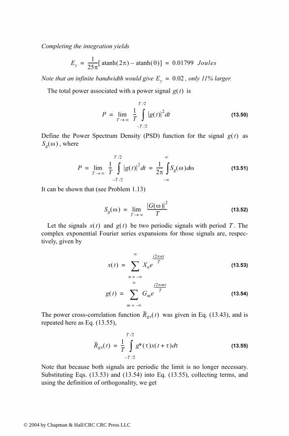
© 200
Completing the integration yields
Note that an infinite bandwidth would give , only 11% larger.
The total power associated with a power signal is
(13.50)
Define the Power Spectrum Density (PSD) function for the signal as , where
(13.51)
It can be shown that (see Problem 1.13)
(13.52)
Let the signals and be two periodic signals with period . The complex exponential Fourier series expansions for those signals are, respec-tively, given by
(13.53)
(13.54)
The power cross-correlation function was given in Eq. (13.43), and is repeated here as Eq. (13.55),
(13.55)
Note that because both signals are periodic the limit is no longer necessary. Substituting Eqs. (13.53) and (13.54) into Eq. (13.55), collecting terms, and using the definition of orthogonality, we get
Ey1
25π--------- 2π( )atanh 0( )atanh[ ] 0.01799 Joules= =
Ey 0.02=
g t( )
P 1T--- g t( ) 2 td
T 2⁄
T 2⁄
∫T ∞→lim=
g t( )Sg ω( )
P 1T--- g t( ) 2 td
T 2⁄
T 2⁄
∫T ∞→lim 1
2π------ Sg ω( ) ωd
∞
∞
∫= =
Sg ω( ) G ω( ) 2
T------------------
T ∞→lim=
x t( ) g t( ) T
x t( ) Xnej2πnt
T--------------
n ∞=
∞
∑=
g t( ) Gmej2πmt
T---------------
m ∞=
∞
∑=
Rgx t( )
Rgx t( ) 1T--- g∗ τ( )x t τ+( ) τd
T 2⁄
T 2⁄
∫=
4 by Chapman & Hall/CRC CRC Press LLC
© 200
(13.56)
When , Eq. (13.56) becomes the power autocorrelation function,
(13.57)
The power spectrum and cross-power spectrum density functions are then computed as the FT of Eqs. (13.57) and (13.56), respectively. More precisely,
(13.58)
The line (or discrete) power spectrum is defined as the plot of versus ,
where the lines are apart. The DC power is , and the total
power is .
13.6. Random VariablesConsider an experiment with outcomes defined by a certain sample space.
The rule or functional relationship that maps each point in this sample space into a real number is called random variable. Random variables are desig-nated by capital letters (e.g., ), and a particular value of a random vari-able is denoted by a lowercase letter (e.g., ).
The Cumulative Distribution Function (cdf) associated with the random vari-able is denoted as , and is interpreted as the total probability that the random variable is less or equal to the value . More precisely,
(13.59)
The probability that the random variable is in the interval is then given by
Rgx t( ) Gn∗Xnej2nπt
T--------------
n ∞=
∞
∑=
x t( ) g t( )=
Rx t( ) Xn2e
j2nπtT
--------------
n ∞=
∞
∑ X02 2 Xn
2ej2nπt
T--------------
n 1=
∞
∑+= =
Sx ω( ) 2π Xn2δ ω 2nπ
T----------
n ∞=
∞
∑=
Sgx ω( ) 2π Gn∗Xnδ ω 2nπT
----------
n ∞=
∞
∑=
Xn2 n
∆f 1 T⁄= X02
Xn2
n ∞=
∞
∑
X Y …, ,x y …, ,
X FX x( )X x
FX x( ) Pr X x≤ =
X x1 x2,( )
4 by Chapman & Hall/CRC CRC Press LLC
© 200
(13.60)
The cdf has the following properties:
(13.61)
It is often practical to describe a random variable by the derivative of its cdf, which is called the Probability Density Function (pdf). The pdf of the random variable is
(13.62)
or, equivalently,
(13.63)
The probability that a random variable has values in the interval is
(13.64)
Define the moment for the random variable as
(13.65)
The first moment, , is called the mean value, while the second moment, , is called the mean squared value. When the random variable
represents an electrical signal across a resistor, then is the DC com-ponent, and is the total average power.
The central moment is defined as
(13.66)
FX x2( ) FX x1( ) Pr x1 X x2≤ ≤ =
0 FX x( ) 1≤ ≤
FX ∞( ) 0=
FX ∞( ) 1=
FX x1( ) FX x2( )≤ x1 x2≤⇔
X
fX x( )xdd FX x( )=
FX x( ) Pr X x≤ fX λ( ) λd
∞
x
∫= =
X x1 x2,( )
FX x2( ) FX x1( ) Pr x1 X x2≤ ≤ fX x( ) xd
x1
x2
∫= =
nth X
E Xn[ ] Xn xnfX x( ) xd
∞
∞
∫= =
E X[ ]E X2[ ] X
1Ω E X[ ]E X2[ ]
nth
E X X( )n
[ ] X X( )n
x x( )nfX x( ) xd
∞
∞
∫= =
4 by Chapman & Hall/CRC CRC Press LLC
© 200
and, thus, the first central moment is zero. The second central moment is called the variance and is denoted by the symbol ,
(13.67)
Appendix 13B has some common pdfs and their means and variances.
In practice, the random nature of an electrical signal may need to be described by more than one random variable. In this case, the joint cdf and pdffunctions need to be considered. The joint cdf and pdf for the two random vari-ables and are, respectively, defined by
(13.68)
(13.69)
The marginal cdfs are obtained as follows:
(13.70)
If the two random variables are statistically independent, then the joint cdfs and pdfs are, respectively, given by
(13.71)
(13.72)
Let us now consider a case when the two random variables and are mapped into two new variables and through some transformations and defined by
(13.73)
The joint pdf, , may be computed based on the invariance of proba-bility under the transformation. One must first compute the matrix of deriva-tives; then the new joint pdf is computed as
(13.74)
σX2
σX2 X X( )
2=
X Y
FXY x y,( ) Pr X x Y y≤;≤ =
fXY x y,( )x y∂
2
∂∂ FXY x y,( )=
FX x( ) fUV u v,( ) ud vd
∞
x
∫∞
∞
∫ FXY x ∞,( )= =
FY y( ) fUV u v,( ) vd ud
∞
y
∫∞
∞
∫ FXY ∞ y,( )= =
FXY x y,( ) FX x( )FY y( )=
fXY x y,( ) fX x( )fY y( )=
X YU V T1
T2
U T1 X Y,( )=
V T2 X Y,( )=
fUV u v,( )
fUV u v,( ) fXY x y,( ) J=
4 by Chapman & Hall/CRC CRC Press LLC
© 200
(13.75)
where the determinant of the matrix of derivatives is called the Jacobian.
The characteristic function for the random variable is defined as
(13.76)
The characteristic function can be used to compute the pdf for a sum of inde-pendent random variables. More precisely, let the random variable be equal to
(13.77)
where is a set of independent random variables. It can be shown that
(13.78)
and the pdf is computed as the inverse Fourier transform of (with the sign of reversed),
(13.79)
The characteristic function may also be used to compute the moment for the random variable as
(13.80)
13.7. Multivariate Gaussian DistributionConsider a joint probability for random variables, . These
variables can be represented as components of an random column vec-tor, . More precisely,
Ju∂∂x
u∂∂y
v∂∂x
v∂∂y
=
J
X
CX ω( ) E ejωX[ ] fX x( )ejωx xd
∞
∞
∫= =
Y
Y X1 X2 … XN+ + +=
Xi ; i 1 …N,=
CY ω( ) CX1ω( )CX2
ω( )…CXNω( )=
fY y( ) CY ω( )y
fY y( ) 12π------ CY ω( )e jωy ωd
∞
∞
∫=
nthX
E Xn[ ] j( )n
ωn
n
d
d CX ω( )ω 0=
=
m X1 X2 … Xm, , ,m 1×
X
4 by Chapman & Hall/CRC CRC Press LLC
© 200
(13.81)
where the superscript indicates the transpose operation. The joint pdf for the vector is
(13.82)
The mean vector is defined as
(13.83)
and the covariance is an matrix given by
(13.84)
Note that if the elements of the vector are independent, then the covariance matrix is a diagonal matrix.
By definition a random vector is multivariate Gaussian if its pdf has the form
(13.85)
where is the mean vector, is the covariance matrix, is inverse of the covariance matrix and is its determinant, and is of dimension . If
is a matrix of rank , then the random vector is a k-variate Gaussian vector with
(13.86)
(13.87)
The characteristic function for a multivariate Gaussian pdf is defined by
(13.88)
Then the moments for the joint distribution can be obtained by partial differen-tiation. For example,
XtX1 X2 … Xm=
X
fx x( ) fx1 x2 … xm, , , x1 x2 … xm, , ,( )=
µx E X1[ ] E X2[ ] … E Xm[ ]t
=
m m×
Cx E X Xt[ ] µx µxt=
X
X
fx x( ) 2π( )m 2⁄ Cx1 2⁄[ ]
1 12--- x µx( )tCx
1 x µx( ) exp=
µx Cx Cx1
Cx X mA k m× k Y AX=
µy Aµx=
Cy ACxAt=
CX E j ω1X1 ω2X2 … ωmXm+ + +( ) exp[ ]
jµxtω 1
2---ωtCxω
exp
= =
4 by Chapman & Hall/CRC CRC Press LLC
© 200
(13.89)
Example:
The vector is a 4-variate Gaussian with
Define
Find the distribution of and the distribution of
Solution:
has a bivariate Gaussian distribution with
The vector can be expressed as
It follows that
E X1X2X3[ ]ω1 ω2∂ ω3∂
3
∂∂ CX ω1 ω2 ω3, ,( )= at ω 0=
X
µx 2 1 1 0t
=
Cx
6 3 2 13 4 3 22 3 4 31 2 3 3
=
X1X1
X2
= X2X3
X4
=
X1
Y2X1
X1 2X2+
X3 X4+
=
X1
µx1
21
= Cx1
6 33 4
=
Y
Y2 0 0 01 2 0 00 0 1 1
X1
X2
X3
X4
AX= =
4 by Chapman & Hall/CRC CRC Press LLC
© 200
13.8. Random ProcessesA random variable is by definition a mapping of all possible outcomes of
a random experiment to numbers. When the random variable becomes a func-tion of both the outcomes of the experiment as well as time, it is called a ran-dom process and is denoted by . Thus, one can view a random process as an ensemble of time domain functions that are the outcome of a certain random experiment, as compared to single real numbers in the case of a random vari-able.
Since the cdf and pdf of a random process are time dependent, we will denote them as and , respectively. The moment for the random process is
(13.90)
A random process is referred to as stationary to order one if all its sta-tistical properties do not change with time. Consequently, , where is a constant. A random process is called stationary to order two (or wide sense stationary) if
(13.91)
for all and .
Define the statistical autocorrelation function for the random process as
(13.92)
The correlation is, in general, a function of . As a con-sequence of the wide sense stationary definition, the autocorrelation function depends on the time difference , rather than on absolute time; and thus, for a wide sense stationary process we have
µy Aµx 4 4 1t
= =
Cy ACxAt24 24 624 34 136 13 13
= =
X
X t( )
FX x t;( ) fX x t;( ) nthX t( )
E Xn t( )[ ] xnfX x t;( ) xd
∞
∞
∫=
X t( )E X t( )[ ] X=
X X t( )
fX x1 x2 t1 t2,;,( ) fX x1 x2 t1 ∆t+ t2 ∆t+,;,( )=
t1 t2, ∆t
X t( )
ℜX t1 t2,( ) E X t1( )X t2( )[ ]=
E X t1( )X t2( )[ ] t1 t2,( )
τ t2 t1=
4 by Chapman & Hall/CRC CRC Press LLC
© 200
(13.93)
If the time average and time correlation functions are equal to the statistical average and statistical correlation functions, the random process is referred to as an ergodic random process. The following is true for an ergodic process:
(13.94)
(13.95)
The covariance of two random processes and is defined by
(13.96)
which can be written as
(13.97)
13.9. Sampling TheoremMost modern communication and radar systems are designed to process dis-
crete samples of signals bearing information. In general, we would like to determine the necessary condition such that a signal can be fully reconstructed from its samples by filtering, or data processing in general. The answer to this question lies in the sampling theorem which may be stated as follows: let the signal be real-valued and band-limited with bandwidth ; this signal can be fully reconstructed from its samples if the time interval between samples is no greater than .
Fig. 13.1 illustrates the sampling process concept. The sampling signal is periodic with period , which is called the sampling interval. The Fourier series expansion of is
(13.98)
The sampled signal is then given by
E X t( )[ ] X=
ℜX τ( ) E X t( )X t τ+( )[ ]=
1T--- x t( ) td
T 2⁄
T 2⁄
∫T ∞→lim E X t( )[ ] X= =
1T--- x∗ t( )x t τ+( ) td
T 2⁄
T 2⁄
∫T ∞→lim ℜX τ( )=
X t( ) Y t( )
CXY t t τ+,( ) E X t( ) E X t( )[ ] Y t τ+( ) E Y t τ+( )[ ] [ ]=
CXY t t τ+,( ) ℜXY τ( ) XY=
x t( ) B
1 2B( )⁄
p t( )Ts
p t( )
p t( ) Pnej2πnt
Ts--------------
n ∞=
∞
∑=
xs t( )
4 by Chapman & Hall/CRC CRC Press LLC
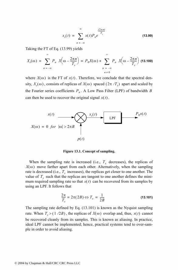
© 200
(13.99)
Taking the FT of Eq. (13.99) yields
(13.100)
where is the FT of . Therefore, we conclude that the spectral den-sity, , consists of replicas of spaced apart and scaled by
the Fourier series coefficients . A Low Pass Filter (LPF) of bandwidth
can then be used to recover the original signal .
When the sampling rate is increased (i.e., decreases), the replicas of move farther apart from each other. Alternatively, when the sampling
rate is decreased (i.e., increases), the replicas get closer to one another. The value of such that the replicas are tangent to one another defines the mini-mum required sampling rate so that can be recovered from its samples by using an LPF. It follows that
(13.101)
The sampling rate defined by Eq. (13.101) is known as the Nyquist sampling rate. When , the replicas of overlap and, thus, cannot be recovered cleanly from its samples. This is known as aliasing. In practice, ideal LPF cannot be implemented; hence, practical systems tend to over-sam-ple in order to avoid aliasing.
xs t( ) x t( )Pnej2πnt
Ts--------------
n ∞=
∞
∑=
Xs ω( ) Pn X ω 2πnTs
----------
n ∞=
∞
∑ P0X ω( ) Pn X ω 2πnTs
----------
n ∞=
n 0≠
∞
∑+= =
X ω( ) x t( )Xs ω( ) X ω( ) 2π Ts⁄( )
Pn B
x t( )
LPF
p t( )
X ω( ) 0 for ω 2πB>=
x t( ) P0x t( )xs t( )
Figure 13.1. Concept of sampling.
TsX ω( )
TsTs
x t( )
2πTs------ 2π 2B( )= Ts⇔ 1
2B-------=
Ts 1 2B⁄( )> X ω( ) x t( )
4 by Chapman & Hall/CRC CRC Press LLC
© 200
Example:
Assume that the sampling signal is given by
Compute an expression for .
Solution:
The signal is called the Comb function. Its exponential Fourier series is
It follows that
Taking the Fourier transform of this equation yields
.
Before proceeding to the next section, we will establish the following nota-tion: samples of the signal are denoted by and referred to as a dis-crete time domain sequence, or simply a sequence. If the signal is periodic, we will denote its sample by the periodic sequence .
13.10. The Z-TransformThe Z-transform is a transformation that maps samples of a discrete time
domain sequence into a new domain known as the z-domain. It is defined as
(13.102)
p t( )
p t( ) δ t nTs( )
n ∞=
∞
∑=
Xs ω( )
p t( )
p t( ) 1Ts-----e
2πntTs
------------
n ∞=
∞
∑=
xs t( ) x t( ) 1Ts-----e
2πntTs
------------
n ∞=
∞
∑=
Xs ω( ) 2πTs------ X ω 2πn
Ts----------
n ∞=
∞
∑=
x t( ) x n( )x t( )
x n( )
Z x n( ) X z( ) x n( )z n
n ∞=
∞
∑= =
4 by Chapman & Hall/CRC CRC Press LLC
© 200
where , and for most cases, . It follows that Eq. (13.102) can be rewritten as
(13.103)
In the z-domain, the region over which is finite is called the Region of Convergence (ROC). Appendix 13C has a list of most common Z-transform pairs. The Z-transform properties are (the proofs are left as an exercise):
1. Linearity:
(13.104)
2. Right-Shifting Property:
(13.105)
3. Left-Shifting Property:
(13.106)
4. Time Scaling:
(13.107)
5. Periodic Sequences:
(13.108)
where is the period.
6. Multiplication by :
(13.109)
7. Division by ; a is a real number:
z rejω= r 1=
X ejω( ) x n( )e jnω
n ∞=
∞
∑=
X z( )
Z ax1 n( ) bx2 n( )+ aX1 z( ) bX2 z( )+=
Z x n k( ) z k X z( )=
Z x n k+( ) zkX z( ) x n( )zk n
n 0=
k 1
∑=
Z anx n( ) X a 1 z( ) a 1 z( )nx n( )
n 0=
∞
∑= =
Z x n( ) zN
zN 1--------------Z x n( ) =
N
n
Z nx n( ) zzdd X z( )=
n a+
4 by Chapman & Hall/CRC CRC Press LLC
© 200
(13.110)
8. Initial Value:
(13.111)
9. Final Value:
(13.112)
10. Convolution:
(13.113)
11. Bilateral Convolution:
(13.114)
Example:
Prove Eq. (13.109).
Solution:
Starting with the definition of the Z-transform,
Taking the derivative, with respect to z, of the above equation yields
Z x n( )n a+------------
x n( )za u k a 1 ud
0
z
∫
n 0=
∞
∑=
x n0( ) zn0X z( ) z ∞→=
x n( )n ∞→lim 1 z 1( )X z( )
z 1→lim=
Z h n k( )x k( )
k 0=
∞
∑
H z( )X z( )=
Z h n k( )x k( )
k ∞=
∞
∑
H z( )X z( )=
X z( ) x
n ∞=
∞
∑ n( )z n=
zdd X z( ) x n( ) n( )
n ∞=
∞
∑ z n 1=
4 by Chapman & Hall/CRC CRC Press LLC
© 200
It follows that
In general, a discrete LTI system has a transfer function which describes how the system operates on its input sequence in order to pro-duce the output sequence . The output sequence is computed from the discrete convolution between the sequences and ,
(13.115)
However, since practical systems require that the sequence be of finite length, we can rewrite Eq. (13.115) as
(13.116)
where denotes the input sequence length. Taking the Z-transform of Eq. (13.116) yields
(13.117)
and the discrete system transfer function is
(13.118)
Finally, the transfer function can be written as
(13.119)
where is the amplitude response, and is the phase response.
z 1( ) nx n( )z n
n ∞=
∞
∑=
Z nx n( ) z( )zdd X z( )=
H z( )x n( )
y n( ) y n( )x n( ) h n( )
y n( ) x m( )h n m( )
m ∞=
∞
∑=
x n( )
y n( ) x m( )h n m( )
m 0=
N
∑=
N
Y z( ) X z( )H z( )=
H z( ) Y z( )X z( )-----------=
H z( )
H z( )z ejω=
H ejω( ) e H ejω( )∠=
H ejω( ) H ejω( )∠
4 by Chapman & Hall/CRC CRC Press LLC
© 200
13.11. The Discrete Fourier TransformThe Discrete Fourier Transform (DFT) is a mathematical operation that
transforms a discrete sequence, usually from the time domain into the fre-quency domain, in order to explicitly determine the spectral information for the sequence. The time domain sequence can be real or complex. The DFT has finite length , and is periodic with period equal to .
The discrete Fourier transform for the finite sequence is defined by
(13.120)
The inverse DFT is given by
(13.121)
The Fast Fourier Transform (FFT) is not a new kind of transform different from the DFT. Instead, it is an algorithm used to compute the DFT more effi-ciently. There are numerous FFT algorithms that can be found in the literature. In this book we will interchangeably use the DFT and the FFT to mean the same thing. Furthermore, we will assume radix-2 FFT algorithm, where the FFT size is equal to for some integer .
13.12. Discrete Power SpectrumPractical discrete systems utilize DFTs of finite length as a means of numer-
ical approximation for the Fourier transform. It follows that input signals must be truncated to a finite duration (denoted by ) before they are sampled. This is necessary so that a finite length sequence is generated prior to signal pro-cessing. Unfortunately, this truncation process may cause some serious prob-lems.
To demonstrate this difficulty, consider the time domain signal . The spectrum of consists of two spectral lines at .
Now, when is truncated to length seconds and sampled at a rate , where is the number of desired samples, we produce the
sequence . The spectrum of would still be composed of the same spectral lines if is an integer multiple of and if the DFT frequency resolution is an integer multiple of . Unfortunately, those two conditions are rarely met and, as a consequence, the spectrum of
N N
x n( )
X k( ) x n( )ej2πnk
N---------------
n 0=
N 1
∑= k; 0 … N 1, ,=
x n( ) 1N---- X k( )e
j2πnkN
---------------
k 0=
N 1
∑= n; 0 … N 1, ,=
N 2m= m
T
x t( ) 2πf0tsin= x t( ) f0±x t( ) T
Ts T N⁄= Nx n( ) n; 0 1 … N 1, , ,= x n( )
T Ts∆f f0
x n( )
4 by Chapman & Hall/CRC CRC Press LLC
© 200
spreads over several lines (normally the spread may extend up to three lines). This is known as spectral leakage. Since is normally unknown, this discon-tinuity caused by an arbitrary choice of cannot be avoided. Windowing tech-niques can be used to mitigate the effect of this discontinuity by applying smaller weights to samples close to the edges.
A truncated sequence can be viewed as one period of some periodic sequence with period . The discrete Fourier series expansion of is
(13.122)
It can be shown that the coefficients are given by
(13.123)
where is the DFT of . Therefore, the Discrete Power Spectrum
(DPS) for the band limited sequence is the plot of versus , where
the lines are apart,
(13.124)
Before proceeding to the next section, we will show how to select the FFT parameters. For this purpose, consider a band limited signal with band-width . If the signal is not band limited, a LPF can be used to eliminate frequencies greater than . In order to satisfy the sampling theorem, one must choose a sampling frequency , such that
(13.125)
The truncated sequence duration and the total number of samples are related by
f0T
x n( )x n( ) N x n( )
x n( ) Xkej2πnk
N---------------
k 0=
N 1
∑=
Xk
Xk1N---- x n( )e
j2πnkN
------------------
n 0=
N 1
∑ 1N----X k( )= =
X k( ) x n( )
x n( ) Xk2 k
∆f
P01
N2------ X 0( ) 2=
Pk1
N2------ X k( ) 2 X N k( ) 2+ = k; 1 2 … N
2---- 1, , ,=
PN 2⁄1
N2------ X N 2⁄( ) 2=
x t( )B
Bfs 1 Ts⁄=
fs 2B≥
T N
4 by Chapman & Hall/CRC CRC Press LLC
© 200
(13.126)
or equivalently,
(13.127)
It follows that
(13.128)
and the frequency resolution is
(13.129)
13.13. Windowing TechniquesTruncation of the sequence can be accomplished by computing the
product,
(13.130)
where
(13.131)
where . The finite sequence is called a windowing sequence, or simply a window. The windowing process should not impact the phase response of the truncated sequence. Consequently, the sequence must retain linear phase. This can be accomplished by making the window symmet-rical with respect to its central point.
If for all we have what is known as the rectangular window. It leads to the Gibbs phenomenon which manifests itself as an overshoot and a ripple before and after a discontinuity. Fig. 13.2 shows the amplitude spectrum of a rectangular window. Note that the first side lobe is at below the main lobe. Windows that place smaller weights on the samples near the edges will have lesser overshoot at the discontinuity points (lower side lobes); hence, they are more desirable than a rectangular window. However, sidelobes reduc-tion is offset by a widening of the main lobe. Therefore, the proper choice of a windowing sequence is continuous trade-off between side lobe reduction and
T NTs=
fsNT----=
fsNT---- 2B≥=
∆f 1NTs---------
fs
N---- 1
T--- 2B
N-------≥= = =
x n( )
xw n( ) x n( )w n( )=
w n( )f n( ) n; 0 1 …, , , N 1=
0 otherwise
=
f n( ) 1≤ w n( )
w n( )
f n( ) 1= n
13.46dB
4 by Chapman & Hall/CRC CRC Press LLC

© 200
main lobe widening. Table 13.1 gives a summary of some windows with the corresponding impact on main beam widening and peak reduction.
The multiplication process defined in Eq. (13.131) is equivalent to cyclic convolution in the frequency domain. It follows that is a smeared (dis-torted) version of . To minimize this distortion, we would seek windows that have a narrow main lobe and small side lobes. Additionally, using a win-dow other than a rectangular window reduces the power by a factor , where
(13.132)
It follows that the DPS for the sequence is now given by
(13.133)
TABLE 13.1. Common windows.
WindowNull-to-null Beamwidth. Rectangular
window is the reference. Peak
Reduction
Rectangular 1 1
Hamming 2 0.73
Hanning 2 0.664
Blackman 6 0.577
Kaiser ( 2.76 0.683
Kaiser ( 1.75 0.882
β 6 )=
β 3 )=
Xw k( )X k( )
Pw
Pw1N---- w2 n( )
n 0=
N 1
∑ W k( ) 2
k 0=
N 1
∑= =
xw n( )
P0w 1
PwN2------------- X 0( ) 2=
Pkw 1
PwN2------------- X k( ) 2 X N k( ) 2+ = k; 1 2 … N
2---- 1, , ,=
PN 2⁄w 1
PwN2------------- X N 2⁄( ) 2=
4 by Chapman & Hall/CRC CRC Press LLC
© 200
where is defined in Eq. (13.132). Table 13.2 lists some common windows. Figs. 13.3 through 13.5 show the frequency domain characteristics for these windows. These figures can be reproduced using MATLAB program figs13.m.
TABLE 13.2. Some common windows.
Window ExpressionFirst side lobe
Main lobe width
rectangular
Hamming
Hanning
Kaiser
is the zero-order modified Bessel function of the first kind
Figure 13.2. Normalized amplitude spectrum for rectangular window.
Pw
n 0 N 1.,=
w n( ) 1= 13.46dB 1
w n( ) 0.54 0.46 2πnN 1------------- cos=
41dB 2
w n( ) 0.5 1 2πnN 1------------- cos=
32dB 2
w n( )I0 β 1 2n N⁄( )2[ ]
I0 β( )-----------------------------------------------=
I0
46dBfor
β
2π=
5forβ 2π=
4 by Chapman & Hall/CRC CRC Press LLC
© 200
Figure 13.3. Normalized amplitude spectrum for Hamming window.
Figure 13.4. Normalized amplitude spectrum for Hanning window.
4 by Chapman & Hall/CRC CRC Press LLC
© 200
13.14. MATLAB Programs
Listing 13.1. MATLAB Program figs13.m%Use this program to reproduce figures in Section 13.13.clear allclose alleps = 0.0001;N = 32;win_rect (1:N) = 1;win_ham = hamming(N);win_han = hanning(N);win_kaiser = kaiser(N, pi);win_kaiser2 = kaiser(N, 5);Yrect = abs(fft(win_rect, 512));Yrectn = Yrect ./ max(Yrect);Yham = abs(fft(win_ham, 512));Yhamn = Yham ./ max(Yham);Yhan = abs(fft(win_han, 512));Yhann = Yhan ./ max(Yhan);
Figure 13.5. Normalized amplitude spectrum for Kaiser window.
4 by Chapman & Hall/CRC CRC Press LLC
© 200
YK = abs(fft(win_kaiser, 512));YKn = YK ./ max(YK);YK2 = abs(fft(win_kaiser2, 512));YKn2 = YK2 ./ max(YK2);figure (1)plot(20*log10(Yrectn+eps),'k')xlabel('Sample number')ylabel('20*log10(amplitude)')axis tightgridfigure(2) plot(20*log10(Yhamn + eps),'k')xlabel('Sample number')ylabel('20*log10(amplitude)')gridaxis tightfigure (3)plot(20*log10(Yhann+eps),'k')xlabel('Sample number')ylabel('20*log10(amplitude)')gridaxis tightfigure(4)plot(20*log10(YKn+eps),'k')gridhold on plot(20*log10(YKn2+eps),'k--')xlabel('Sample number')ylabel('20*log10(amplitude)')legend('Kaiser par. = \pi','Kaiser par. =5') axis tighthold off
4 by Chapman & Hall/CRC CRC Press LLC
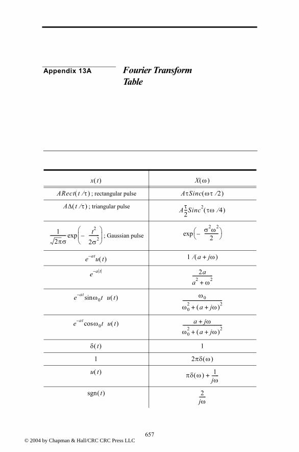
© 200
Appendix 13A Fourier Transform Table
; rectangular pulse
; triangular pulse
; Gaussian pulse
x t( ) X ω( )
ARect t τ⁄( ) AτSinc ωτ 2⁄( )
A∆ t τ⁄( ) Aτ2---Sinc2 τω 4⁄( )
12πσ
-------------- t2
2σ2---------
expσ2ω2
2------------
exp
e at u t( ) 1 a jω+( )⁄
e a t 2aa2 ω2+------------------
e at ω0tsin u t( ) ω0
ω02 a jω+( )2+
-----------------------------------
e at ω0cos t u t( ) a jω+
ω02 a jω+( )2+
-----------------------------------
δ t( ) 1
1 2πδ ω( )
u t( ) πδ ω( ) 1jω------+
t( )sgn 2jω------
6574 by Chapman & Hall/CRC CRC Press LLC
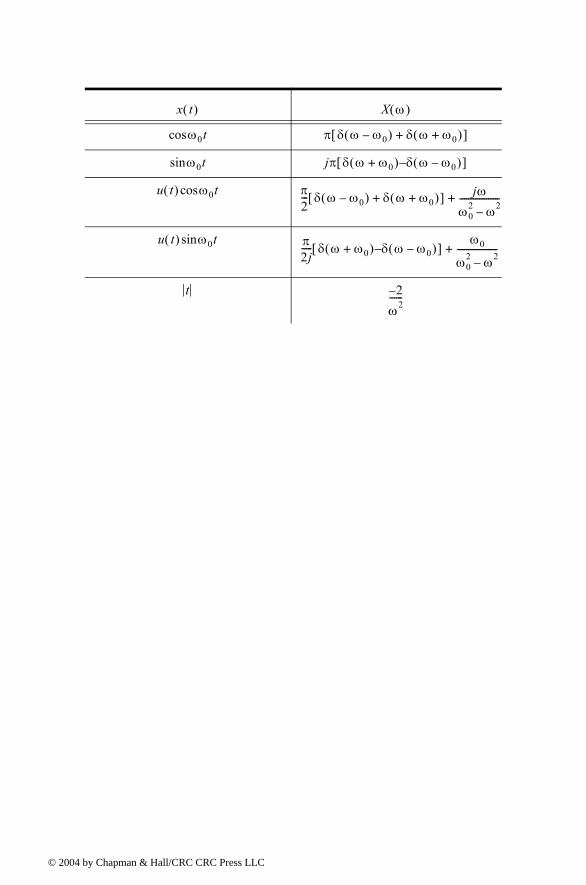
© 200
x t( ) X ω( )
ω0tcos π δ ω ω0( ) δ ω ω0+( )+[ ]
ω0tsin jπ δ ω ω0+( ) δ ω ω0( )[ ]
u t( ) ω0tcos π2--- δ ω ω0( ) δ ω ω0+( )+[ ] jω
ω02 ω2
------------------+
u t( ) ω0tsin π2j----- δ ω ω0+( ) δ ω ω0( )[ ]
ω0
ω02 ω2
------------------+
t 2
ω2------
4 by Chapman & Hall/CRC CRC Press LLC
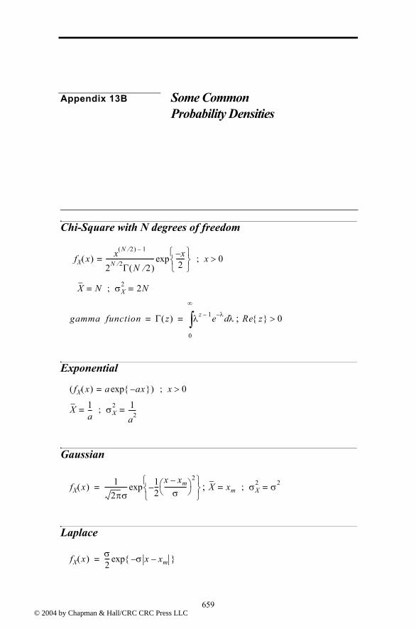
© 200
Appendix 13B Some Common Probability Densities
Chi-Square with N degrees of freedom
;
Exponential
Gaussian
;
Laplace
fX x( ) x N 2⁄( ) 1
2N 2⁄ Γ N 2⁄( )------------------------------- x
2-----
exp= x 0>;
X N= σX2; 2N=
gamma function Γ z( ) λz 1 e λ λd
0
∞
∫= = Re z 0>
fX x( ) a ax exp=( ) x 0>;
X 1a---= σX
2; 1a2-----=
fX x( ) 12πσ
-------------- 12---
x xm
σ--------------
2
exp= X xm= σX2; σ2=
fX x( ) σ2--- σ x xm exp=
6594 by Chapman & Hall/CRC CRC Press LLC
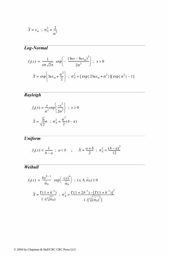
© 200
Log-Normal
Rayleigh
Uniform
;
Weibull
X xm= σX2; 2
σ2-----=
fX x( ) 1xσ 2π-----------------
xln xmln( )2
2σ2---------------------------------
exp x 0>;=
X xmln σ2
2-----+
exp= σX2; 2 xmln σ2+ exp[ ] σ2 exp 1[ ]=
fX x( ) xσ2----- x2
2σ2---------
exp= x 0≥;
X π2---σ= σX
2;σ2
2----- 4 π( )=
fX x( ) 1b a------------= a b<; X a b+
2------------= σX
2; b a( )2
12-------------------=
fX x( ) bxb 1
σ0-------------- x( )b
σ0---------
x b σ0, ,( ) 0≥;exp=
X Γ 1 b 1+( )
1 σ0b( )⁄
-------------------------= σX2; Γ 1 2b 1+( ) Γ 1 b 1+( )[ ]
2
1 σ0( )2b[ ]⁄
--------------------------------------------------------------------=
4 by Chapman & Hall/CRC CRC Press LLC
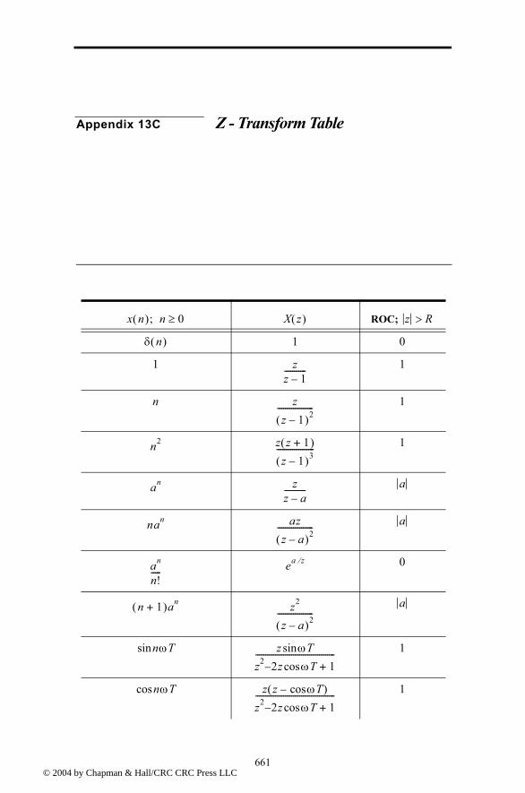
© 200
Appendix 13C Z - Transform Table
ROC; x n( ) n 0≥; X z( ) z R>
δ n( ) 1 0
1 zz 1----------- 1
n zz 1( )2------------------ 1
n2 z z 1+( )
z 1( )3------------------- 1
an zz a----------- a
nan azz a( )2------------------ a
an
n!----- ea z⁄ 0
n 1+( )an z2
z a( )2------------------
a
nωTsin z ωTsinz2 2z ωTcos 1+---------------------------------------- 1
nωTcos z z ωTcos( )
z2 2z ωTcos 1+---------------------------------------- 1
6614 by Chapman & Hall/CRC CRC Press LLC
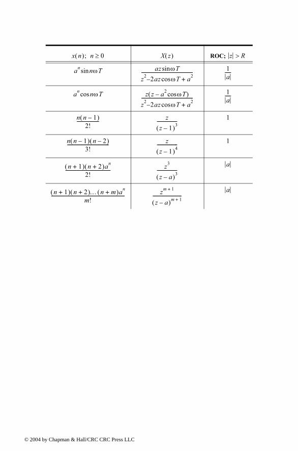
© 200
ROC; x n( ) n 0≥; X z( ) z R>
an nωTsin az ωTsinz2 2az ωTcos a2+---------------------------------------------- 1
a-----
an nωTcos z z a2 ωTcos( )
z2 2az ωTcos a2+----------------------------------------------
1a-----
n n 1( )2!
-------------------- zz 1( )3------------------ 1
n n 1( ) n 2( )3!
------------------------------------- zz 1( )4------------------ 1
n 1+( ) n 2+( )an
2!---------------------------------------- z3
z a( )3------------------
a
n 1+( ) n 2+( )… n m+( )an
m!----------------------------------------------------------------- zm 1+
z a( )m 1+--------------------------
a
4 by Chapman & Hall/CRC CRC Press LLC
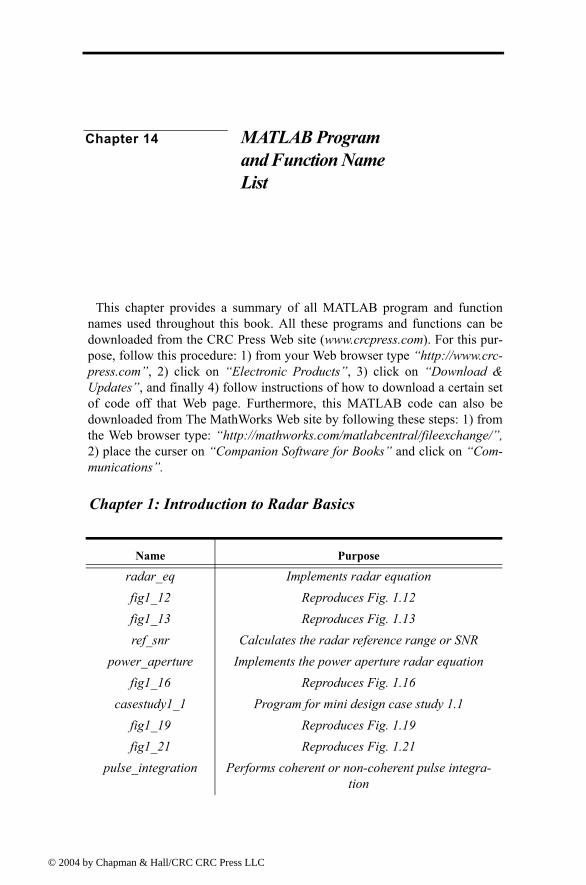
© 200
Chapter 14 MATLAB Program and Function Name List
This chapter provides a summary of all MATLAB program and function names used throughout this book. All these programs and functions can be downloaded from the CRC Press Web site (www.crcpress.com). For this pur-pose, follow this procedure: 1) from your Web browser type http://www.crc-press.com, 2) click on Electronic Products, 3) click on Download & Updates, and finally 4) follow instructions of how to download a certain set of code off that Web page. Furthermore, this MATLAB code can also be downloaded from The MathWorks Web site by following these steps: 1) from the Web browser type: http://mathworks.com/matlabcentral/fileexchange/, 2) place the curser on Companion Software for Books and click on Com-munications.
Chapter 1: Introduction to Radar Basics
Name Purpose
radar_eq Implements radar equationfig1_12 Reproduces Fig. 1.12fig1_13 Reproduces Fig. 1.13ref_snr Calculates the radar reference range or SNR
power_aperture Implements the power aperture radar equationfig1_16 Reproduces Fig. 1.16
casestudy1_1 Program for mini design case study 1.1fig1_19 Reproduces Fig. 1.19fig1_21 Reproduces Fig. 1.21
pulse_integration Performs coherent or non-coherent pulse integra-tion
4 by Chapman & Hall/CRC CRC Press LLC
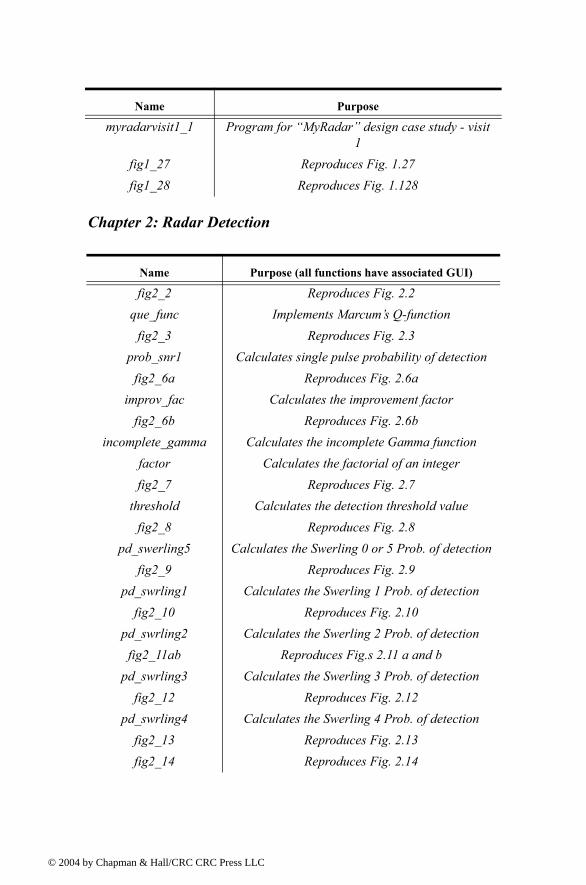
© 200
Chapter 2: Radar Detection
myradarvisit1_1 Program for MyRadar design case study - visit 1
fig1_27 Reproduces Fig. 1.27fig1_28 Reproduces Fig. 1.128
Name Purpose (all functions have associated GUI)
fig2_2 Reproduces Fig. 2.2que_func Implements Marcums Q-function
fig2_3 Reproduces Fig. 2.3prob_snr1 Calculates single pulse probability of detection
fig2_6a Reproduces Fig. 2.6aimprov_fac Calculates the improvement factor
fig2_6b Reproduces Fig. 2.6bincomplete_gamma Calculates the incomplete Gamma function
factor Calculates the factorial of an integerfig2_7 Reproduces Fig. 2.7
threshold Calculates the detection threshold valuefig2_8 Reproduces Fig. 2.8
pd_swerling5 Calculates the Swerling 0 or 5 Prob. of detectionfig2_9 Reproduces Fig. 2.9
pd_swrling1 Calculates the Swerling 1 Prob. of detectionfig2_10 Reproduces Fig. 2.10
pd_swrling2 Calculates the Swerling 2 Prob. of detectionfig2_11ab Reproduces Fig.s 2.11 a and b
pd_swrling3 Calculates the Swerling 3 Prob. of detectionfig2_12 Reproduces Fig. 2.12
pd_swrling4 Calculates the Swerling 4 Prob. of detectionfig2_13 Reproduces Fig. 2.13fig2_14 Reproduces Fig. 2.14
Name Purpose
4 by Chapman & Hall/CRC CRC Press LLC
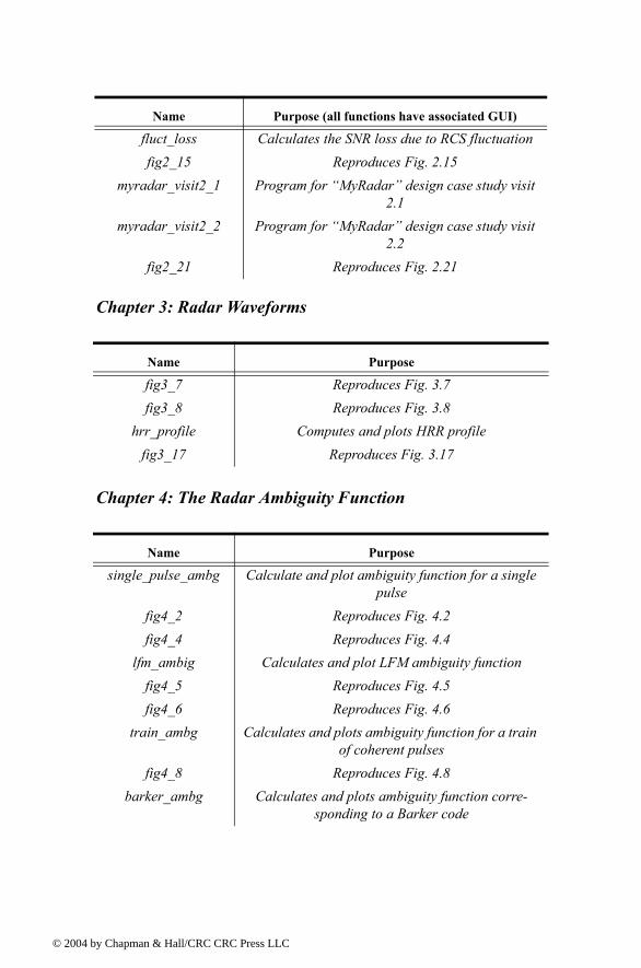
© 200
Chapter 3: Radar Waveforms
Chapter 4: The Radar Ambiguity Function
fluct_loss Calculates the SNR loss due to RCS fluctuationfig2_15 Reproduces Fig. 2.15
myradar_visit2_1 Program for MyRadar design case study visit 2.1
myradar_visit2_2 Program for MyRadar design case study visit 2.2
fig2_21 Reproduces Fig. 2.21
Name Purpose
fig3_7 Reproduces Fig. 3.7fig3_8 Reproduces Fig. 3.8
hrr_profile Computes and plots HRR profilefig3_17 Reproduces Fig. 3.17
Name Purpose
single_pulse_ambg Calculate and plot ambiguity function for a single pulse
fig4_2 Reproduces Fig. 4.2fig4_4 Reproduces Fig. 4.4
lfm_ambig Calculates and plot LFM ambiguity functionfig4_5 Reproduces Fig. 4.5fig4_6 Reproduces Fig. 4.6
train_ambg Calculates and plots ambiguity function for a train of coherent pulses
fig4_8 Reproduces Fig. 4.8barker_ambg Calculates and plots ambiguity function corre-
sponding to a Barker code
Name Purpose (all functions have associated GUI)
4 by Chapman & Hall/CRC CRC Press LLC
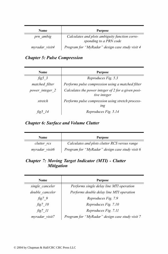
© 200
Chapter 5: Pulse Compression
Chapter 6: Surface and Volume Clutter
Chapter 7: Moving Target Indicator (MTI) - Clutter Mitigation
prn_ambig Calculates and plots ambiguity function corre-sponding to a PRN code
myradar_visit4 Program for MyRadar design case study visit 4
Name Purpose
fig5_3 Reproduces Fig. 5.3matched_filter Performs pulse compression using a matched filter
power_integer_2 Calculates the power integer of 2 for a given posi-tive integer
stretch Performs pulse compression using stretch process-ing
fig5_14 Reproduces Fig. 5.14
Name Purpose
clutter_rcs Calculates and plots clutter RCS versus rangemyradar_visit6 Program for MyRadar design case study visit 6
Name Purpose
single_canceler Performs single delay line MTI operationdouble_canceler Performs double delay line MTI operation
fig7_9 Reproduces Fig. 7.9fig7_10 Reproduces Fig. 7.10fig7_11 Reproduces Fig. 7.11
myradar_visit7 Program for MyRadar design case study visit 7
Name Purpose
4 by Chapman & Hall/CRC CRC Press LLC
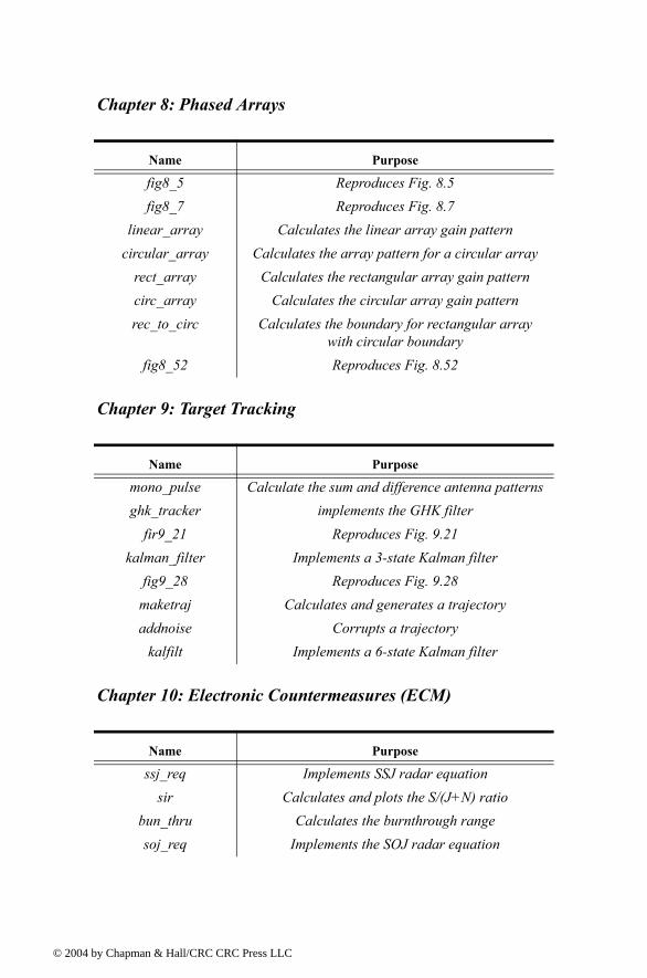
© 200
Chapter 8: Phased Arrays
Chapter 9: Target Tracking
Chapter 10: Electronic Countermeasures (ECM)
Name Purpose
fig8_5 Reproduces Fig. 8.5fig8_7 Reproduces Fig. 8.7
linear_array Calculates the linear array gain patterncircular_array Calculates the array pattern for a circular array
rect_array Calculates the rectangular array gain patterncirc_array Calculates the circular array gain patternrec_to_circ Calculates the boundary for rectangular array
with circular boundaryfig8_52 Reproduces Fig. 8.52
Name Purpose
mono_pulse Calculate the sum and difference antenna patternsghk_tracker implements the GHK filter
fir9_21 Reproduces Fig. 9.21kalman_filter Implements a 3-state Kalman filter
fig9_28 Reproduces Fig. 9.28maketraj Calculates and generates a trajectoryaddnoise Corrupts a trajectory
kalfilt Implements a 6-state Kalman filter
Name Purpose
ssj_req Implements SSJ radar equationsir Calculates and plots the S/(J+N) ratio
bun_thru Calculates the burnthrough rangesoj_req Implements the SOJ radar equation
4 by Chapman & Hall/CRC CRC Press LLC
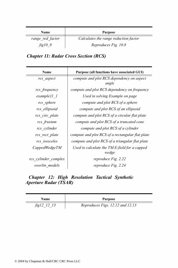
© 200
Chapter 11: Radar Cross Section (RCS)
Chapter 12: High Resolution Tactical Synthetic Aperture Radar (TSAR)
range_red_factor Calculates the range reduction factorfig10_8 Reproduces Fig. 10.8
Name Purpose (all functions have associated GUI)
rcs_aspect compute and plot RCS dependency on aspect angle
rcs_frequency compute and plot RCS dependency on frequencyexample11_1 Used in solving Example on page rcs_sphere compute and plot RCS of a sphere
rcs_ellipsoid compute and plot RCS of an ellipsoidrcs_circ_plate compute and plot RCS of a circular flat platercs_frustum compute and plot RCS of a truncated conercs_cylinder compute and plot RCS of a cylinder
rcs_rect_plate compute and plot RCS of a rectangular flat platercs_isosceles compute and plot RCS of a triangular flat plate
CappedWedgeTM Used to calculate the TM E-field for a capped wedge
rcs_cylinder_complex reproduce Fig. 2.22swerlin_models reproduce Fig. 2.24
Name Purpose
fig12_12_13 Reproduces Figs. 12.12 and 12.13
Name Purpose
4 by Chapman & Hall/CRC CRC Press LLC

© 200
Chapter 13: Signal Processing
Name Purpose
figs13 Reproduces Fig. 13.2 through Fig. 13.5.
4 by Chapman & Hall/CRC CRC Press LLC
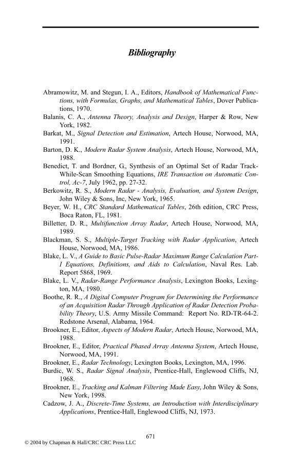
© 200
Bibliography
Abramowitz, M. and Stegun, I. A., Editors, Handbook of Mathematical Func-tions, with Formulas, Graphs, and Mathematical Tables, Dover Publica-tions, 1970.
Balanis, C. A., Antenna Theory, Analysis and Design, Harper & Row, New York, 1982.
Barkat, M., Signal Detection and Estimation, Artech House, Norwood, MA, 1991.
Barton, D. K., Modern Radar System Analysis, Artech House, Norwood, MA, 1988.
Benedict, T. and Bordner, G., Synthesis of an Optimal Set of Radar Track-While-Scan Smoothing Equations, IRE Transaction on Automatic Con-trol, Ac-7, July 1962, pp. 27-32.
Berkowitz, R. S., Modern Radar - Analysis, Evaluation, and System Design, John Wiley & Sons, Inc, New York, 1965.
Beyer, W. H., CRC Standard Mathematical Tables, 26th edition, CRC Press, Boca Raton, FL, 1981.
Billetter, D. R., Multifunction Array Radar, Artech House, Norwood, MA, 1989.
Blackman, S. S., Multiple-Target Tracking with Radar Application, Artech House, Norwood, MA, 1986.
Blake, L. V., A Guide to Basic Pulse-Radar Maximum Range Calculation Part-I Equations, Definitions, and Aids to Calculation, Naval Res. Lab. Report 5868, 1969.
Blake, L. V., Radar-Range Performance Analysis, Lexington Books, Lexing-ton, MA, 1980.
Boothe, R. R., A Digital Computer Program for Determining the Performance of an Acquisition Radar Through Application of Radar Detection Proba-bility Theory, U.S. Army Missile Command: Report No. RD-TR-64-2. Redstone Arsenal, Alabama, 1964.
Brookner, E., Editor, Aspects of Modern Radar, Artech House, Norwood, MA, 1988.
Brookner, E., Editor, Practical Phased Array Antenna System, Artech House, Norwood, MA, 1991.
Brookner, E., Radar Technology, Lexington Books, Lexington, MA, 1996.Burdic, W. S., Radar Signal Analysis, Prentice-Hall, Englewood Cliffs, NJ,
1968.Brookner, E., Tracking and Kalman Filtering Made Easy, John Wiley & Sons,
New York, 1998.Cadzow, J. A., Discrete-Time Systems, an Introduction with Interdisciplinary
Applications, Prentice-Hall, Englewood Cliffs, NJ, 1973.
6714 by Chapman & Hall/CRC CRC Press LLC
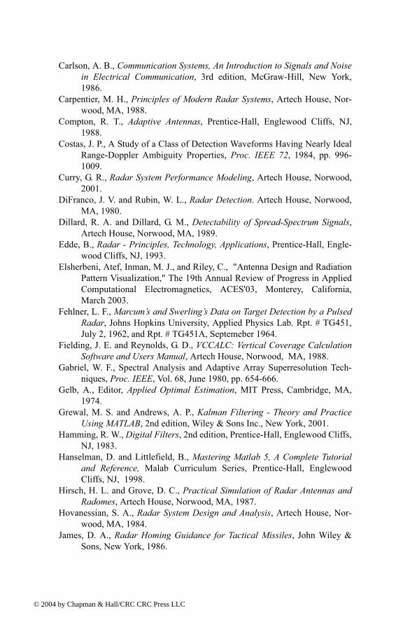
© 200
Carlson, A. B., Communication Systems, An Introduction to Signals and Noise in Electrical Communication, 3rd edition, McGraw-Hill, New York, 1986.
Carpentier, M. H., Principles of Modern Radar Systems, Artech House, Nor-wood, MA, 1988.
Compton, R. T., Adaptive Antennas, Prentice-Hall, Englewood Cliffs, NJ, 1988.
Costas, J. P., A Study of a Class of Detection Waveforms Having Nearly Ideal Range-Doppler Ambiguity Properties, Proc. IEEE 72, 1984, pp. 996-1009.
Curry, G. R., Radar System Performance Modeling, Artech House, Norwood, 2001.
DiFranco, J. V. and Rubin, W. L., Radar Detection. Artech House, Norwood, MA, 1980.
Dillard, R. A. and Dillard, G. M., Detectability of Spread-Spectrum Signals, Artech House, Norwood, MA, 1989.
Edde, B., Radar - Principles, Technology, Applications, Prentice-Hall, Engle-wood Cliffs, NJ, 1993.
Elsherbeni, Atef, Inman, M. J., and Riley, C., "Antenna Design and Radiation Pattern Visualization," The 19th Annual Review of Progress in Applied Computational Electromagnetics, ACES'03, Monterey, California, March 2003.
Fehlner, L. F., Marcums and Swerlings Data on Target Detection by a Pulsed Radar, Johns Hopkins University, Applied Physics Lab. Rpt. # TG451, July 2, 1962, and Rpt. # TG451A, Septemeber 1964.
Fielding, J. E. and Reynolds, G. D., VCCALC: Vertical Coverage Calculation Software and Users Manual, Artech House, Norwood, MA, 1988.
Gabriel, W. F., Spectral Analysis and Adaptive Array Superresolution Tech-niques, Proc. IEEE, Vol. 68, June 1980, pp. 654-666.
Gelb, A., Editor, Applied Optimal Estimation, MIT Press, Cambridge, MA, 1974.
Grewal, M. S. and Andrews, A. P., Kalman Filtering - Theory and Practice Using MATLAB, 2nd edition, Wiley & Sons Inc., New York, 2001.
Hamming, R. W., Digital Filters, 2nd edition, Prentice-Hall, Englewood Cliffs, NJ, 1983.
Hanselman, D. and Littlefield, B., Mastering Matlab 5, A Complete Tutorial and Reference, Malab Curriculum Series, Prentice-Hall, Englewood Cliffs, NJ, 1998.
Hirsch, H. L. and Grove, D. C., Practical Simulation of Radar Antennas and Radomes, Artech House, Norwood, MA, 1987.
Hovanessian, S. A., Radar System Design and Analysis, Artech House, Nor-wood, MA, 1984.
James, D. A., Radar Homing Guidance for Tactical Missiles, John Wiley & Sons, New York, 1986.
4 by Chapman & Hall/CRC CRC Press LLC

© 200
Kanter, I., Exact Detection Probability for Partially Correlated Rayleigh Targets, IEEE Trans. AES-22, pp. 184-196. March 1986.
Kay, S. M., Fundamentals of Statistical Signal Processing - Estimation Theory, Volume I, Prentice Hall Signal Processing Series, New Jersey, 1993.
Kay, S. M., Fundamentals of Statistical Signal Processing - Detection Theory, Volume II, Prentice Hall Signal Processing Series, New Jersey, 1993.
Klauder, J. R., Price, A. C., Darlington, S., and Albershiem, W. J., The Theory and Design of Chirp Radars, The Bell System Technical Journal, Vol. 39, No. 4, 1960.
Knott, E. F., Shaeffer, J. F., and Tuley, M. T., Radar Cross Section, 2nd edition, Artech House, Norwood, MA, 1993.
Lativa, J., Low-Angle Tracking Using Multifrequency Sampled Aperture Radar, IEEE - AES Trans., Vol. 27, No. 5, September 1991, pp.797-805.
Levanon, N., Radar Principles, John Wiley & Sons, New York, 1988.Lewis, B. L., Kretschmer, Jr., F. F., and Shelton, W. W., Aspects of Radar Sig-
nal Processing, Artech House, Norwood, MA, 1986.Long, M. W., Radar Reflectivity of Land and Sea, Artech House, Norwood,
MA, 1983.Lothes, R. N., Szymanski, M. B., and Wiley, R. G., Radar Vulnerability to Jam-
ming, Artech House, Norwood, MA, 1990.Mahafza, B. R. and Polge, R. J., Multiple Target Detection Through DFT Pro-
cessing in a Sequential Mode Operation of Real Two-Dimensional Arrays, Proc. of the IEEE Southeast Conf. '90, New Orleans, LA, April 1990, pp. 168-170.
Mahafza, B. R., Heifner, L.A., and Gracchi, V. C., Multitarget Detection Using Synthetic Sampled Aperture Radars (SSAMAR), IEEE - AES Trans., Vol. 31, No. 3, July 1995, pp. 1127-1132.
Mahafza, B. R. and Sajjadi, M., Three-Dimensional SAR Imaging Using a Linear Array in Transverse Motion, IEEE - AES Trans., Vol. 32, No. 1, January 1996, pp. 499-510.
Mahafza, B. R., Introduction to Radar Analysis, CRC Press, Boca Raton, FL, 1998.
Mahafza, B. R., Radar Systems Analysis and Design Using MATLAB, CRC Press, Boca Raton, FL, 2000.
Marchand, P., Graphics and GUIs with Matlab, 2nd edition, CRC Press, Boca Raton, FL, 1999.
Marcum, J. I., A Statistical Theory of Target Detection by Pulsed Radar, Math-ematical Appendix, IRE Trans., Vol. IT-6, April 1960, pp. 59-267.
Meeks, M. L., Radar Propagation at Low Altitudes, Artech House, Norwood, MA, 1982.
Melsa, J. L. and Cohn, D. L., Decision and Estimation Theory, McGraw-Hill, New York, 1978.
Mensa, D. L., High Resolution Radar Imaging, Artech House, Norwood, MA, 1984.
4 by Chapman & Hall/CRC CRC Press LLC
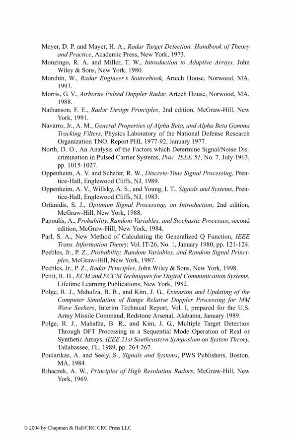
© 200
Meyer, D. P. and Mayer, H. A., Radar Target Detection: Handbook of Theory and Practice, Academic Press, New York, 1973.
Monzingo, R. A. and Miller, T. W., Introduction to Adaptive Arrays, John Wiley & Sons, New York, 1980.
Morchin, W., Radar Engineers Sourcebook, Artech House, Norwood, MA, 1993.
Morris, G. V., Airborne Pulsed Doppler Radar, Artech House, Norwood, MA, 1988.
Nathanson, F. E., Radar Design Principles, 2nd edition, McGraw-Hill, New York, 1991.
Navarro, Jr., A. M., General Properties of Alpha Beta, and Alpha Beta Gamma Tracking Filters, Physics Laboratory of the National Defense Research Organization TNO, Report PHL 1977-92, January 1977.
North, D. O., An Analysis of the Factors which Determine Signal/Noise Dis-crimination in Pulsed Carrier Systems, Proc. IEEE 51, No. 7, July 1963, pp. 1015-1027.
Oppenheim, A. V. and Schafer, R. W., Discrete-Time Signal Processing, Pren-tice-Hall, Englewood Cliffs, NJ, 1989.
Oppenheim, A. V., Willsky, A. S., and Young, I. T., Signals and Systems, Pren-tice-Hall, Englewood Cliffs, NJ, 1983.
Orfanidis, S. J., Optimum Signal Processing, an Introduction, 2nd edition, McGraw-Hill, New York, 1988.
Papoulis, A., Probability, Random Variables, and Stochastic Processes, second edition, McGraw-Hill, New York, 1984.
Parl, S. A., New Method of Calculating the Generalized Q Function, IEEE Trans. Information Theory, Vol. IT-26, No. 1, January 1980, pp. 121-124.
Peebles, Jr., P. Z., Probability, Random Variables, and Random Signal Princi-ples, McGraw-Hill, New York, 1987.
Peebles, Jr., P. Z., Radar Principles, John Wiley & Sons, New York, 1998.Pettit, R. H., ECM and ECCM Techniques for Digital Communication Systems,
Lifetime Learning Publications, New York, 1982.Polge, R. J., Mahafza, B. R., and Kim, J. G., Extension and Updating of the
Computer Simulation of Range Relative Doppler Processing for MM Wave Seekers, Interim Technical Report, Vol. I, prepared for the U.S. Army Missile Command, Redstone Arsenal, Alabama, January 1989.
Polge, R. J., Mahafza, B. R., and Kim, J. G., Multiple Target Detection Through DFT Processing in a Sequential Mode Operation of Real or Synthetic Arrays, IEEE 21st Southeastern Symposium on System Theory, Tallahassee, FL, 1989, pp. 264-267.
Poularikas, A. and Seely, S., Signals and Systems, PWS Publishers, Boston, MA, 1984.
Rihaczek, A. W., Principles of High Resolution Radars, McGraw-Hill, New York, 1969.
4 by Chapman & Hall/CRC CRC Press LLC

© 200
Ross, R. A., Radar Cross Section of Rectangular Flat Plate as a Function of Aspect Angle, IEEE Trans. AP-14:320, 1966.
Ruck, G. T., Barrick, D. E., Stuart, W. D., and Krichbaum, C. K., Radar Cross Section Handbook, Volume 1, Plenum Press, New York, 1970.
Ruck, G. T., Barrick, D. E., Stuart, W. D., and Krichbaum, C. K., Radar Cross Section Handbook, Volume 2, Plenum Press, New York, 1970.
Rulf, B. and Robertshaw, G. A., Understanding Antennas for Radar, Communi-cations, and Avionics, Van Nostrand Reinhold, 1987.
Scanlan, M.J., Editor, Modern Radar Techniques, Macmillan, New York, 1987.Scheer, J. A. and Kurtz, J. L., Editors, Coherent Radar Performance Estima-
tion, Artech House, Norwood, MA, 1993.Shanmugan, K. S. and Breipohl, A. M., Random Signals: Detection, Estima-
tion and Data Analysis, John Wiley & Sons, New York, 1988.Sherman, S. M., Monopulse Principles and Techniques, Artech House, Nor-
wood, MA.Singer, R. A., Estimating Optimal Tracking Filter Performance for Manned
Maneuvering Targets, IEEE Transaction on Aerospace and Electronics, AES-5, July 1970, pp. 473-483.
Skillman, W. A., DETPROB: Probability of Detection Calculation Software and Users Manual, Artech House, Norwood, MA, 1991.
Skolnik, M. I., Introduction to Radar Systems, McGraw-Hill, New York, 1982.Skolnik, M. I., Editor, Radar Handbook, 2nd edition, McGraw-Hill, New
York, 1990.Stearns, S. D. and David, R. A., Signal Processing Algorithms, Prentice-Hall,
Englewood Cliffs, NJ, 1988.Stimson, G. W., Introduction to Airborne Radar, Hughes Aircaft Company, El
Segundo, CA, 1983.Stratton, J. A., Electromagnetic Theory, McGraw-Hill, New York, 1941.Stremler, F. G., Introduction to Communication Systems, 3rd edition, Addison-
Wesley, New York, 1990.Stutzman, G. E., Estimating Directivity and Gain of Antennas, IEEE Antennas
and Propagation Magazine 40, August 1998, pp 7-11.Swerling, P., Probability of Detection for Fluctuating Targets, IRE Transaction on
Information Theory, Vol IT-6, April 1960, pp. 269-308.Van Trees, H. L., Detection, Estimation, and Modeling Theory, Part I. Wiley & Sons,
Inc., New York, 2001.Van Trees, H. L., Detection, Estimation, and Modeling Theory, Part III.Wiley & Sons,
Inc., New York, 2001.Van Trees, H. L., Optimum Array Processing, Part IV of Detection, Estimation, and
Modeling Theory, Wiley & Sons, Inc., New York, 2002.Tzannes, N. S., Communication and Radar Systems, Prentice-Hall, Englewood
Cliffs, NJ, 1985.Urkowtiz, H., Signal Theory and Random Processes, Artech House, Norwood,
MA, 1983.
4 by Chapman & Hall/CRC CRC Press LLC

© 200
Urkowitz, H., Decision and Detection Theory, Unpublished Lecture Notes, Lockheed Martin Co., Moorestown, NJ.
Vaughn, C. R., Birds and Insects as Radar Targets: A Review, Proc. IEEE, Vol. 73, No. 2, February 1985, pp. 205-227.
Wehner, D. R., High Resolution Radar, Artech House, Norwood, MA, 1987.White, J. E., Mueller, D. D., and Bate, R. R., Fundamentals of Astrodynamics,
Dover Publications, 1971.Ziemer, R. E. and Tranter, W. H., Principles of Communications, Systems,
Modulation, and Noise, 2nd edition, Houghton Mifflin, Boston, MA, 1985.
Zierler, N., Several Binary-Sequence Generators, MIT Technical Report No. 95, Sept. 1955.
4 by Chapman & Hall/CRC CRC Press LLC