Embed Size (px)
Citation preview
11
Polynomials and Curve Fitting
Lecture Series – 5
by
Shameer Koya
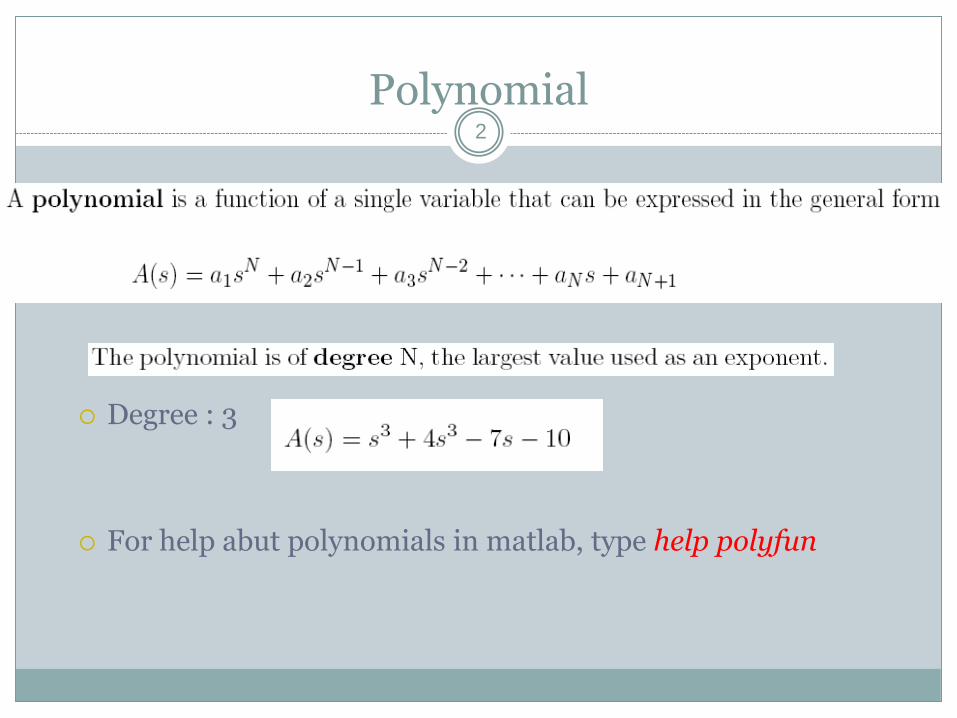
Polynomial
Degree : 3
For help abut polynomials in matlab, type help polyfun
2

Polynomials in MATLAB
MATLAB provides a number of functions for themanipulation of polynomials. These include, Evaluation of polynomials
Finding roots of polynomials
Addition, subtraction, multiplication, and division of polynomials
Dealing with rational expressions of polynomials
Curve fitting
Polynomials are defined in MATLAB as row vectors made up of thecoefficients of the polynomial, whose dimension is n+1, n being thedegree of the polynomial
p = [1 -12 0 25 116] represents x4 - 12x3 + 25x + 116
3

Roots
>>p = [1, -12, 0, 25, 116]; % 4th order polynomial
>>r = roots(p)
r =
11.7473
2.7028
-1.2251 + 1.4672i
-1.2251 - 1.4672i
From a set of roots we can also determine the polynomial
>>pp = poly(r)
r =
1 -12 -1.7764e-014 25 116
4

Addition and Subtraction
MATLAB does not provide a direct function for adding or subtracting polynomials unless they are of the same order, when they are of the same order, normal matrix addition and subtraction applies, d = a + b and e = a – b are defined when a and b are of the same order.
When they are not of the same order, the lesser order polynomial must be padded with leading zeroes before adding or subtracting the two polynomials.
>>p1=[3 15 0 -10 -3 15 -40];
>>p2 = [3 0 -2 -6];
>>p = p1 + [0 0 0 p2];
>>p =
3 15 0 -7 -3 13 -46
The lesser polynomial is padded and then added or subtracted as appropriate.
5
Multiplication
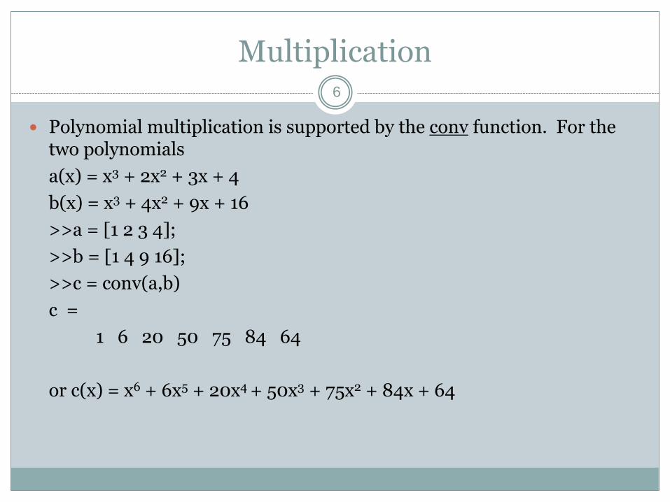
Polynomial multiplication is supported by the conv function. For the two polynomials
a(x) = x3 + 2x2 + 3x + 4
b(x) = x3 + 4x2 + 9x + 16
>>a = [1 2 3 4];
>>b = [1 4 9 16];
>>c = conv(a,b)
c =
1 6 20 50 75 84 64
or c(x) = x6 + 6x5 + 20x4 + 50x3 + 75x2 + 84x + 64
6
Multiplication II
Couple observations, Multiplication of more than two polynomials requires repeated
use of the conv function.
Polynomials need not be of the same order to use the convfunction.
Remember that functions can be nested so conv(conv(a,b),c) makes sense.
7
Division
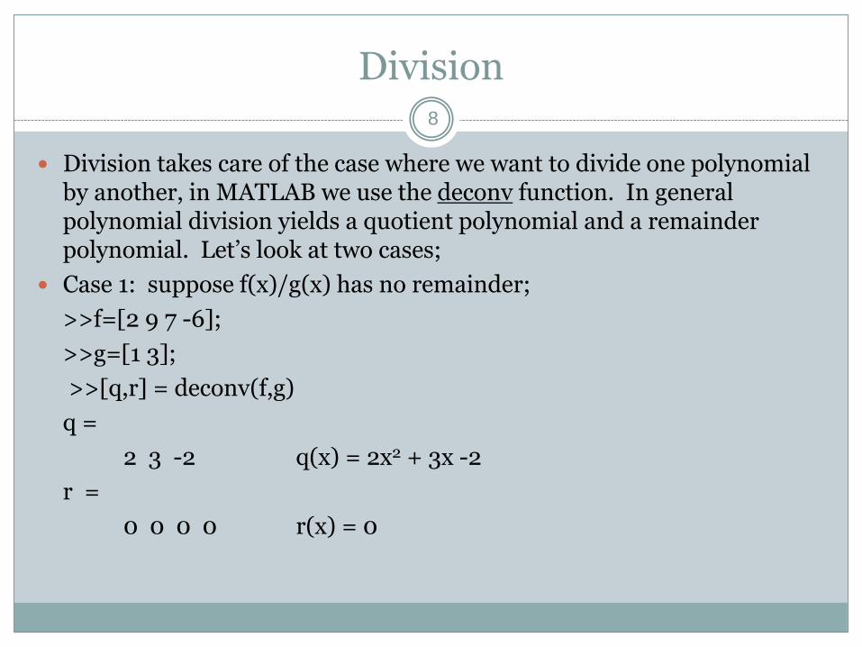
Division takes care of the case where we want to divide one polynomial by another, in MATLAB we use the deconv function. In general polynomial division yields a quotient polynomial and a remainder polynomial. Let’s look at two cases;
Case 1: suppose f(x)/g(x) has no remainder;
>>f=[2 9 7 -6];
>>g=[1 3];
>>[q,r] = deconv(f,g)
q =
2 3 -2 q(x) = 2x2 + 3x -2
r =
0 0 0 0 r(x) = 0
8
Division II
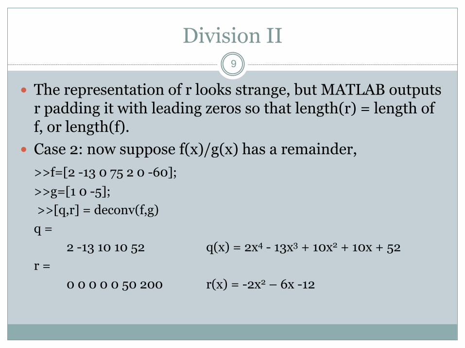
The representation of r looks strange, but MATLAB outputs r padding it with leading zeros so that length(r) = length of f, or length(f).
Case 2: now suppose f(x)/g(x) has a remainder,
>>f=[2 -13 0 75 2 0 -60];
>>g=[1 0 -5];
>>[q,r] = deconv(f,g)
q =
2 -13 10 10 52 q(x) = 2x4 - 13x3 + 10x2 + 10x + 52
r =
0 0 0 0 0 50 200 r(x) = -2x2 – 6x -12
9

Derivatives
Derivative of
Single polynomial
k = polyder(p)
Product of polynomials
k = polyder(a,b)
Quotient of two polynomials
[n d] = polyder(u,v)
10
Evaluation
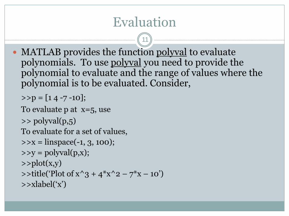
MATLAB provides the function polyval to evaluate polynomials. To use polyval you need to provide the polynomial to evaluate and the range of values where the polynomial is to be evaluated. Consider,
>>p = [1 4 -7 -10];
To evaluate p at x=5, use
>> polyval(p,5)
To evaluate for a set of values,
>>x = linspace(-1, 3, 100);
>>y = polyval(p,x);
>>plot(x,y)
>>title(‘Plot of x^3 + 4*x^2 – 7*x – 10’)
>>xlabel(‘x’)
11
Curve Fitting
MATLAB provides a number of ways to fit a curve to a set of measured data. One of these methods uses the “least squares” curve fit. This technique minimizes the squared errors between the curve and the set of measured data.
The function polyfit solves the least squares polynomial curve fitting problem.
To use polyfit, we must supply the data and the order or degree of the polynomial we wish to best fit to the data. For n = 1, the best fit straight line is found, this is called linear regression. For n = 2 a quadratic polynomial will be found.
12

Curve Fitting II
Consider the following example; Suppose you take 11 measurements of some physical system, each spaced 0.1 seconds apart from 0 to 1 sec. Let x be the row vector specifying the time values, and y the row vector of the actual measurements.
>>x = [0 .1 .2 .3 .4 .5 .6 .7 .8 .9 1];
>>y = [-.447 1.978 3.28 6.16 7.08 7.34 7.66 9.56 9.48 9.30 11.2];
>>n = 2;
>>p = polyfit( x, y, n ) %Find the best quadratic fit to the data
p =
-9.8108 20.1293 -0.317
or p(x) = -9.8108x2 + 20.1293 – 0.317
13

Curve Fitting ....
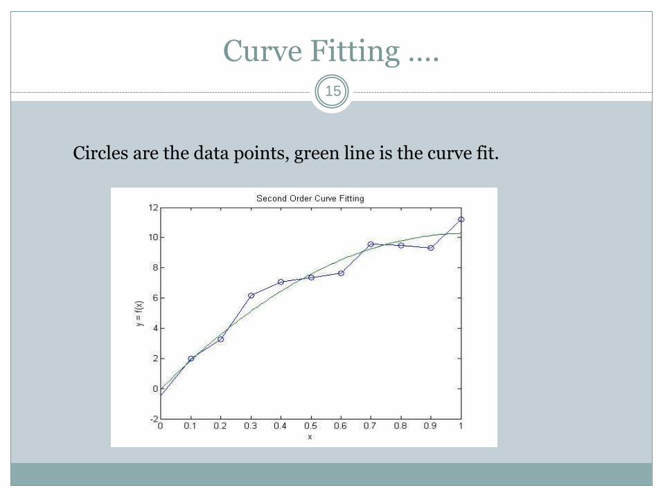
Let’s check out our least squares quadratic vs the measurement data to see how well polyfit performed.
>>xi = linspace(0,1,100);
>>yi = polyval(p, xi);
>>plot(x,y,’-o’, xi, yi, ‘-’)
>>xlabel(‘x’), ylabel(‘y = f(x)’)
>>title(‘Second Order Curve Fitting Example’)
14
Curve Fitting ….
Circles are the data points, green line is the curve fit.
15

Polynomial fit (degree 2)
Start with polynomial of degree 2 (i.e. quadratic):
p=polyfit(x,y,2)
p =
-0.0040 -0.0427 0.3152
So the polynomial is -0.0040x2 - 0.0427x + 0.3152
Could this be much use? Calculate the points using polyval and then plot...
yi=polyval(p,xi);
plot(x,y,’d’,xi,yi)
16

Polynomial fit (degree 2)17
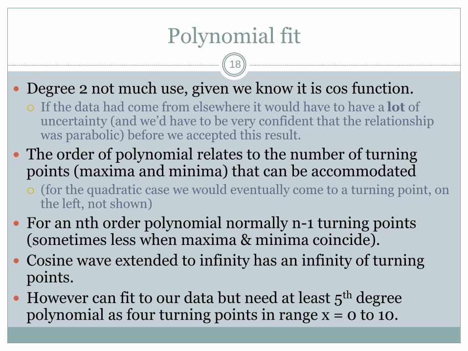
Polynomial fit
Degree 2 not much use, given we know it is cos function. If the data had come from elsewhere it would have to have a lot of
uncertainty (and we’d have to be very confident that the relationship was parabolic) before we accepted this result.
The order of polynomial relates to the number of turning points (maxima and minima) that can be accommodated (for the quadratic case we would eventually come to a turning point, on
the left, not shown)
For an nth order polynomial normally n-1 turning points (sometimes less when maxima & minima coincide).
Cosine wave extended to infinity has an infinity of turning points.
However can fit to our data but need at least 5th degree polynomial as four turning points in range x = 0 to 10.
18
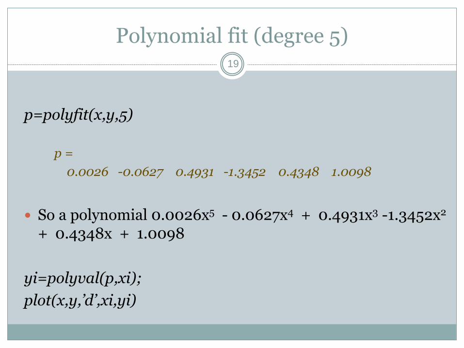
Polynomial fit (degree 5)
p=polyfit(x,y,5)
p =
0.0026 -0.0627 0.4931 -1.3452 0.4348 1.0098
So a polynomial 0.0026x5 - 0.0627x4 + 0.4931x3 -1.3452x2
+ 0.4348x + 1.0098
yi=polyval(p,xi);
plot(x,y,’d’,xi,yi)
19
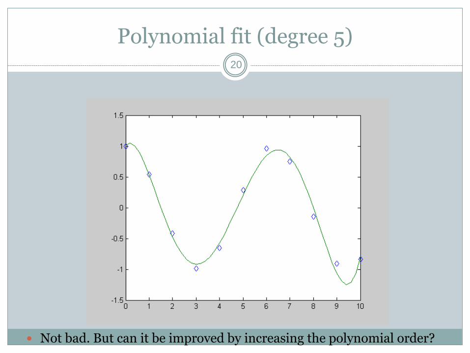
Polynomial fit (degree 5)
Not bad. But can it be improved by increasing the polynomial order?
20

Polynomial fit (degree 8)
plot(x,y,'d',xi,yi,'b',xi,cos(xi),'r')
agreement is now quite good (even better if we go to degree 9)
21

Summary of Polynomial Functions22
Function Description
conv Multiply polynomials
deconv Divide polynomials
poly Polynomial with specified roots
polyder Polynomial derivative
polyfit Polynomial curve fitting
polyval Polynomial evaluation
polyvalm Matrix polynomial evaluation
residue Partial-fraction expansion (residues)
roots Find polynomial roots

23
Thanks
Questions ??


![Indian Institute of Technology (ISM) Dhanbad Dhanbad, … · 2021. 1. 11. · Numerial solution of PDE using MATLAB. [9] Module 7: Polynomial curve fitting. Curve fitting using MATLAB](https://img.pdfslide.us/doc/110x75/6119cfbbd2890a0396172093/indian-institute-of-technology-ism-dhanbad-dhanbad-2021-1-11-numerial-solution.jpg)