Embed Size (px)
Citation preview

DEVELOPMENT OF A 2D HYDRAULIC MODEL FOR
THE RHINE VALLEY USING OPEN DATA
AUTHOR:
MARTIJN KRIEBEL
24/06/2016
BSc Thesis – Martijn Kriebel ii
Development of a 2D hydraulic model for the Rhine valley
using open data
BSc thesis for the bachelor’s programme Civil Engineering at the Faculty of Engineering Technology of the
University of Twente, combined with an internship at Deltares.
Author: Martijn Kriebel s1441043 [email protected]
Completion date: June 24th 2016
Supervisors:
Deltares: Prof. dr. J.C.J. Kwadijk
Ir. M. Hegnauer
University of Twente: Ir. K.D. Berends
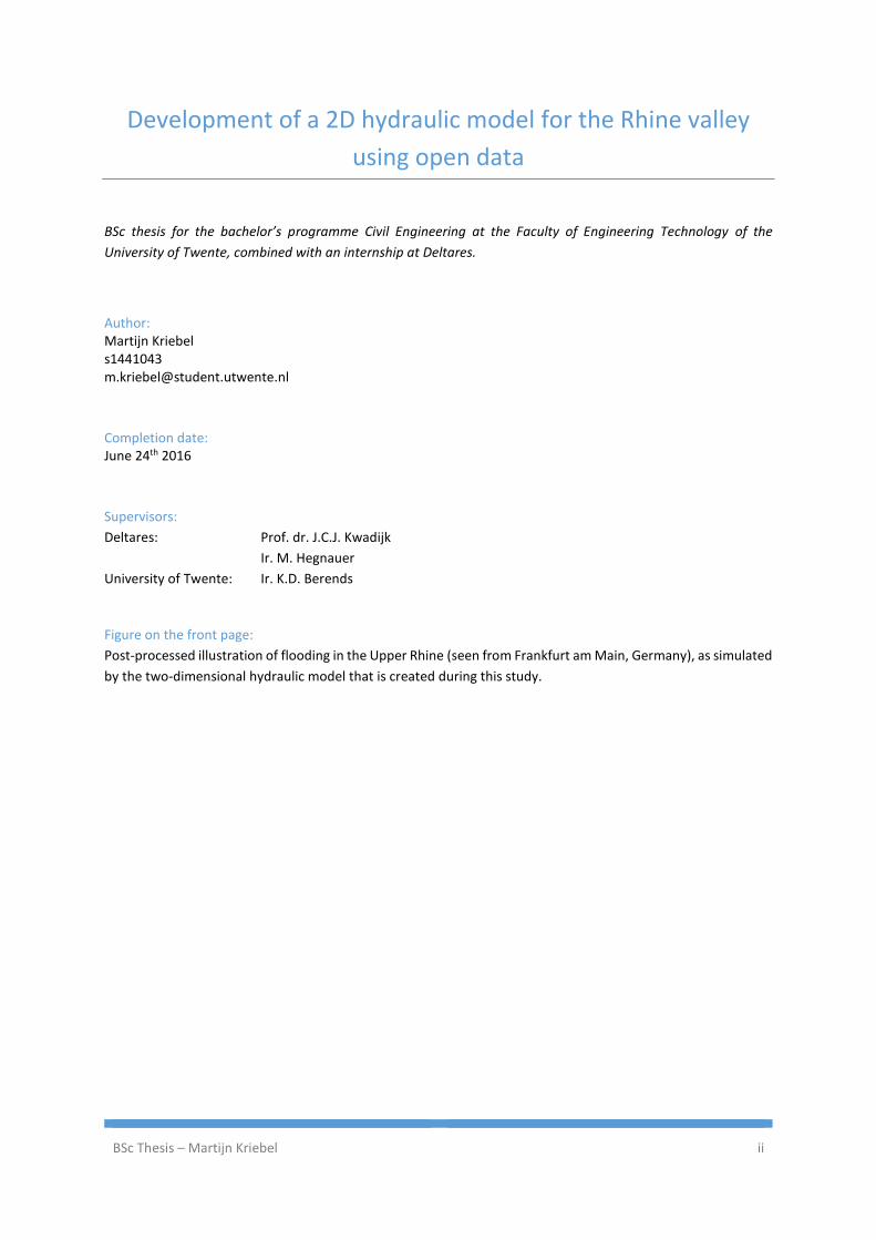
Figure on the front page:
Post-processed illustration of flooding in the Upper Rhine (seen from Frankfurt am Main, Germany), as simulated
by the two-dimensional hydraulic model that is created during this study.
Development of a 2D hydraulic model for the Rhine valley using open data iii
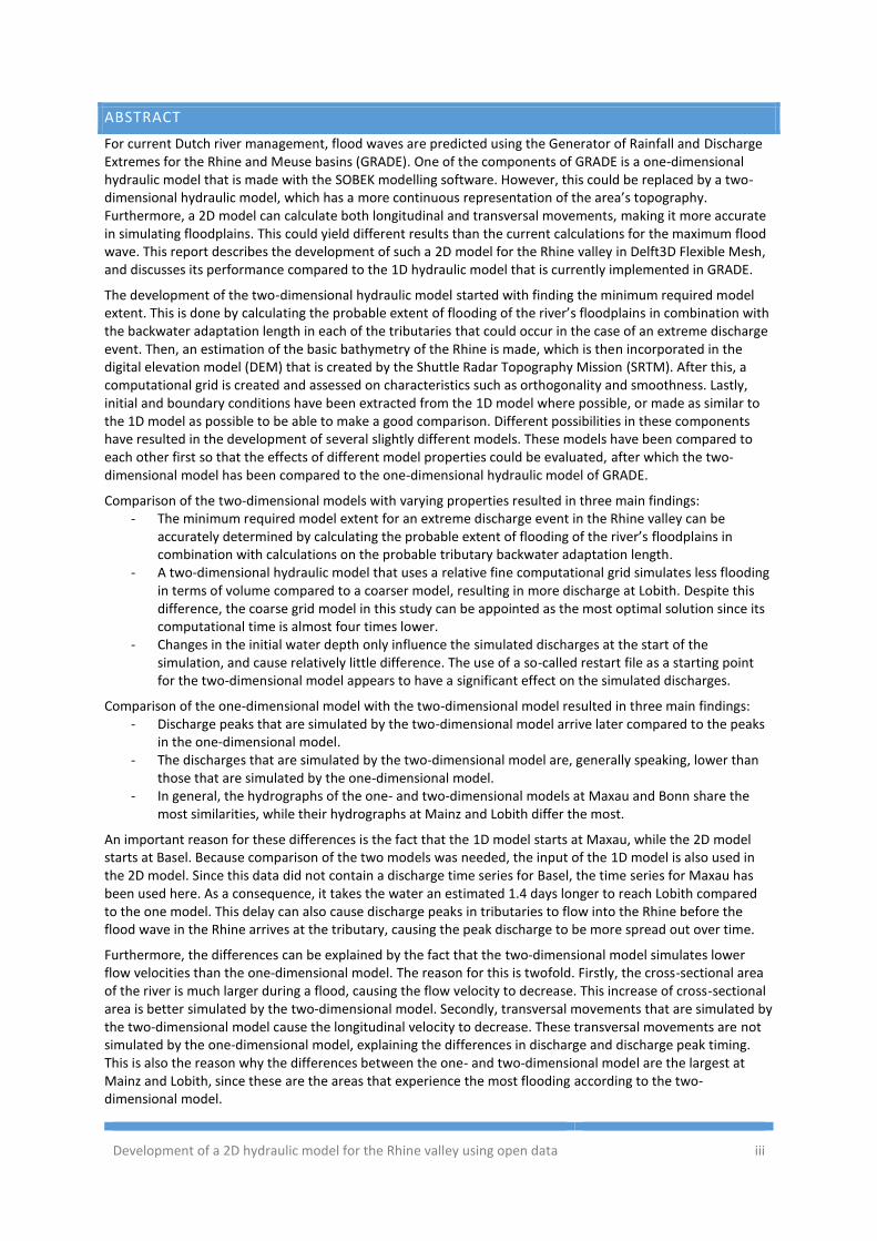
ABSTRACT
For current Dutch river management, flood waves are predicted using the Generator of Rainfall and Discharge Extremes for the Rhine and Meuse basins (GRADE). One of the components of GRADE is a one-dimensional hydraulic model that is made with the SOBEK modelling software. However, this could be replaced by a two-dimensional hydraulic model, which has a more continuous representation of the area’s topography. Furthermore, a 2D model can calculate both longitudinal and transversal movements, making it more accurate in simulating floodplains. This could yield different results than the current calculations for the maximum flood wave. This report describes the development of such a 2D model for the Rhine valley in Delft3D Flexible Mesh, and discusses its performance compared to the 1D hydraulic model that is currently implemented in GRADE.
The development of the two-dimensional hydraulic model started with finding the minimum required model extent. This is done by calculating the probable extent of flooding of the river’s floodplains in combination with the backwater adaptation length in each of the tributaries that could occur in the case of an extreme discharge event. Then, an estimation of the basic bathymetry of the Rhine is made, which is then incorporated in the digital elevation model (DEM) that is created by the Shuttle Radar Topography Mission (SRTM). After this, a computational grid is created and assessed on characteristics such as orthogonality and smoothness. Lastly, initial and boundary conditions have been extracted from the 1D model where possible, or made as similar to the 1D model as possible to be able to make a good comparison. Different possibilities in these components have resulted in the development of several slightly different models. These models have been compared to each other first so that the effects of different model properties could be evaluated, after which the two-dimensional model has been compared to the one-dimensional hydraulic model of GRADE.
Comparison of the two-dimensional models with varying properties resulted in three main findings: - The minimum required model extent for an extreme discharge event in the Rhine valley can be
accurately determined by calculating the probable extent of flooding of the river’s floodplains in combination with calculations on the probable tributary backwater adaptation length.
- A two-dimensional hydraulic model that uses a relative fine computational grid simulates less flooding in terms of volume compared to a coarser model, resulting in more discharge at Lobith. Despite this difference, the coarse grid model in this study can be appointed as the most optimal solution since its computational time is almost four times lower.
- Changes in the initial water depth only influence the simulated discharges at the start of the simulation, and cause relatively little difference. The use of a so-called restart file as a starting point for the two-dimensional model appears to have a significant effect on the simulated discharges.
Comparison of the one-dimensional model with the two-dimensional model resulted in three main findings: - Discharge peaks that are simulated by the two-dimensional model arrive later compared to the peaks
in the one-dimensional model. - The discharges that are simulated by the two-dimensional model are, generally speaking, lower than
those that are simulated by the one-dimensional model. - In general, the hydrographs of the one- and two-dimensional models at Maxau and Bonn share the
most similarities, while their hydrographs at Mainz and Lobith differ the most.
An important reason for these differences is the fact that the 1D model starts at Maxau, while the 2D model starts at Basel. Because comparison of the two models was needed, the input of the 1D model is also used in the 2D model. Since this data did not contain a discharge time series for Basel, the time series for Maxau has been used here. As a consequence, it takes the water an estimated 1.4 days longer to reach Lobith compared to the one model. This delay can also cause discharge peaks in tributaries to flow into the Rhine before the flood wave in the Rhine arrives at the tributary, causing the peak discharge to be more spread out over time.
Furthermore, the differences can be explained by the fact that the two-dimensional model simulates lower flow velocities than the one-dimensional model. The reason for this is twofold. Firstly, the cross-sectional area of the river is much larger during a flood, causing the flow velocity to decrease. This increase of cross-sectional area is better simulated by the two-dimensional model. Secondly, transversal movements that are simulated by the two-dimensional model cause the longitudinal velocity to decrease. These transversal movements are not simulated by the one-dimensional model, explaining the differences in discharge and discharge peak timing. This is also the reason why the differences between the one- and two-dimensional model are the largest at Mainz and Lobith, since these are the areas that experience the most flooding according to the two-dimensional model.

BSc Thesis – Martijn Kriebel iv
PREFACE
The thesis that lies before you is the result of an internship from April to June 2016 at Deltares, and is submitted
in partial fulfilment of the requirements for a Bachelor’s Degree in Civil Engineering at the University of Twente.
This report describes the development of a two-dimensional hydraulic model for the Rhine valley, and discusses
its performance compared to the one-dimensional hydraulic model that is currently in use.
During this short, but interesting period I had the opportunity to develop my academic skills as well as my
knowledge of this field of civil engineering. I am grateful to everyone who helped me completing this study and
thesis. I would like to express my appreciation to Jaap Kwadijk, who gave me the opportunity to work on this
subject in the first place, and to Mark Hegnauer, who provided me with guidance and advice during the
internship. I am also thankful to Koen Berends, who gave me valuable feedback on both my research proposal
and thesis and who guided me through the process of writing them. Furthermore, I would like to thank Anke
Becker who was always available for help when modelling problems arose. Lastly, I want to thank all the other
interns at Deltares who provided me with useful advice and feedback, and with whom I had a pleasant time at
the office.
Martijn Kriebel
Delft, June 24th 2016
Development of a 2D hydraulic model for the Rhine valley using open data v
TABLE OF CONTENTS
Abstract ................................................................................................................................................................... iii
Preface .................................................................................................................................................................... iv
1. Introduction ........................................................................................................................................................ 1
1.1. Background information and problem definition ........................................................................................ 1
1.2. Study area .................................................................................................................................................... 2
1.3. Research questions ...................................................................................................................................... 2
1.4. Thesis outline ............................................................................................................................................... 3
1.5. Software and open data ............................................................................................................................... 3
2. Theoretical background ...................................................................................................................................... 4
3. Methodology ....................................................................................................................................................... 6
3.1. Model extent ................................................................................................................................................ 6
3.1.1. Floodplains ............................................................................................................................................ 6
3.1.2. Tributary backwater .............................................................................................................................. 9
3.1.3. Final model extent .............................................................................................................................. 11
3.2. Model geometry ......................................................................................................................................... 12
3.2.1. DEM interpolation ............................................................................................................................... 12
3.2.2. Bathymetry .......................................................................................................................................... 13
3.3. Computational grid .................................................................................................................................... 13
3.3.1. Main channel and floodplain grid ....................................................................................................... 14
3.3.2. Tributary grid ....................................................................................................................................... 15
3.3.3. Irregularities ........................................................................................................................................ 16
3.3.4. Grid characteristics.............................................................................................................................. 17
3.3.5. Final grid .............................................................................................................................................. 17
3.4. Initial conditions ......................................................................................................................................... 18
3.5. Boundary conditions .................................................................................................................................. 18
3.5.1. Upstream boundary condition ............................................................................................................ 18
3.5.2. Downstream boundary condition ....................................................................................................... 19
3.6. Numerical properties ................................................................................................................................. 21
3.6.1. Conveyance and cell elevation ............................................................................................................ 21
3.6.2. Courant number .................................................................................................................................. 21
4. Results ............................................................................................................................................................... 22
4.1. Model domain ............................................................................................................................................ 23
4.2. Grid ............................................................................................................................................................. 24
4.3. Initial water depth ...................................................................................................................................... 27
4.4. Initial discharges ......................................................................................................................................... 27
BSc Thesis – Martijn Kriebel vi
4.5. 2D Delft3D FM model vs. 1D SOBEK model ............................................................................................... 28
5. Discussion .......................................................................................................................................................... 32
6. Conclusions ....................................................................................................................................................... 33
7. Recommendations ............................................................................................................................................ 34
References ............................................................................................................................................................ 35
Appendices ............................................................................................................................................................ 37
A. Study area ..................................................................................................................................................... 37
B. Rhine sections based on slope linearity ........................................................................................................ 38
C. Indicative floodplains Upper Rhine ............................................................................................................... 39
D. Indicative floodplains Middle Rhine ............................................................................................................. 40
E. Indicative floodplains Lower Rhine ............................................................................................................... 41
F. Tributary slopes ............................................................................................................................................. 42
G. Model extent ................................................................................................................................................ 45
H. Orthogonality of coarse grid ......................................................................................................................... 46
I. Orthogonality of fine grid ............................................................................................................................... 47
J. Smoothness of coarse grid ............................................................................................................................. 48
K. Smoothness of fine grid ................................................................................................................................ 49
L. Average water depth in the Rhine ................................................................................................................. 50
M. Downstream boundary conditions .............................................................................................................. 51
N. Locations of hydrographs ............................................................................................................................. 52
Development of a 2D hydraulic model for the Rhine valley using open data 1
1. INTRODUCTION
1.1. BACKGROUND INFORMATION AND PROBLEM DEFINITION
The Netherlands is a country that is inextricably connected to water, and has a history of many flooding events.
As much of the country covers the estuaries of the rivers Rhine, Meuse and Scheldt, 29% of its territory is
susceptible to river flooding (Reuters, 2010). Even though the Dutch Ministry of Infrastructure and the
Environment tries to lower the risk of river floods (with projects like “Ruimte voor de Rivier”), dykes are still
crucial for protecting the part of the population that lives near rivers. These dykes are designed to withstand
extreme discharges. For the Netherlands, river dykes should be able to withstand discharges that occur once
every 1250 years. For the river Rhine this would correspond to a discharge of 16050 m3/s at Lobith (Chbab, 1995).
Modifying and improving these dykes is a very costly operation. It is estimated that in order to raise a dyke 50
centimeter over a length of 1 kilometer, an investment of 2 million euro is needed. Furthermore, an estimated
total investment over the period 2015-2050 of 3.5 billion euro is needed to improve dyke safety (Kind, 2008).
This shows that investing in more accurate discharge estimations is justified given the costs of raising a dyke.
There is an ongoing debate about the maximum discharge that can arrive at the gauging station of Lobith, where
the Rhine exits Germany and enters the Netherlands. An underestimation of the discharge in the case of such
flood wave could lead to a disaster with many victims, but an overestimation on the other hand could result in
raising the dykes and thus unnecessary expenses.
For current Dutch river management, flood waves are predicted using the Generator of Rainfall and Discharge
Extremes for the Rhine and Meuse basins (GRADE), which has been developed by the Royal Netherlands
Meteorological Institute (KNMI) and Deltares. GRADE consists of three major components:
1. Stochastic weather generator: a generator which has been developed by KNMI. It produces daily rainfall
and temperature series which are based on historical data.
2. Hydrologiska Byråns Vattenbalansavdelning (HBV) model: a hydrological model that calculates the
runoff that occurs as a consequence of the simulated precipitation and temperature series.
3. 1D SOBEK model: a 1D hydraulic model of the Rhine, made with the river/estuary version of the SOBEK
modelling software (SOBEK-RE). By selecting the annual maximum discharges (which are the
consequence of the runoff that has been calculated with the HBV model), annual maximum flood waves
can be simulated. Using these flood waves, possible flooding of the area surrounding the Rhine can be
simulated. For the Rhine, a SOBEK model from Maxau (Germany) to Lobith is used.
(Hegnauer, Beersma, van den Boogaard, Buishand, & Passchier, 2014)
A one-dimensional model such as the SOBEK model in GRADE describes the river geometry using several cross-
sections that are perpendicular to the flow. Furthermore, the model’s boundary conditions consist of
hydrographs that are supplied by the HBV model and a downstream water level time series at Lobith. At each
cross-section and for each time step, the model computes water levels and discharges using the flow equations
for mass and momentum. This gives an indication of how the flood wave propagates through the Rhine river and
eventually how high the discharges are that arrive at Lobith. However, there are two problems with this method.
A first complication is the fact that calculated data (like water level surface) needs to be interpolated between
cross-sections, which leads to uncertainties in between them. Additionally, this information is highly dependent
on the chosen location of the cross-sections, as Bates and De Roo (2000) remark.
Another problem arises when one wants to model a river flood wave which should include floodplains. Maddock,
Harby, Kemp and Wood (2013) state that 1D models cannot accurately predict a flood wave with large lateral in-
and outflows, as is the case when floodplains are flooded. This can be explained by the fact that a one-
BSc Thesis – Martijn Kriebel 2
dimensional model is only able to provide flow properties in the downstream direction, while in- and outflows
between the river and floodplains are also caused by transversal movements. As a consequence of this, one-
dimensional models are known to consider low-lying floodplain areas that are not connected to the main channel
as flooded, because the elevation of these areas is lower than the interpolated water level surface (Werner,
2000).
These problems could be solved by using a two-dimensional model, since such a model has a more continuous
representation of the area’s topography. Furthermore, a 2D model can simulate both longitudinal and transversal
movements, and is therefore able to simulate floodplains more accurate than one-dimensional models. This
could yield different calculation results for the maximum flood wave.
In order to create such a 2D model, a Digital Elevation Model (DEM) is needed. In the beginning of the year 2000
NASA started publishing high-resolution topographic data of the Earth between 60° north and 56° south latitude,
which is approximately 80% of the Earth’s total landmass (Jet Propulsion Laboratory, 2015). This data was
collected during the Shuttle Radar Topography Mission (SRTM). Initially the highest resolution data (1-arc second,
or circa 30 meter) was only available for the United States while the data for the rest of the world had a lower
resolution of 3-arc second (circa 90 meter). However, at the end of 2014 and beginning of 2015, global 1-arc
second elevation data became publically accessible (Jet Propulsion Laboratory, 2014). The fact that this kind of
accurate, topographic data of the whole world is publically accessible, combined with the increase of computer
power the last decades opens the door to more comprehensive hydraulic models.
This report describes how a two-dimensional hydraulic model of the Rhine has been created using the SRTM
DEM data. Furthermore, it analyses the impact of several model aspects on the results, and discusses the
differences between this 2D model and the 1D SOBEK model of GRADE when an extreme discharge event is
simulated.
1.2. STUDY AREA
The study area of this study is the valley of the Rhine from Basel (Switzerland, located along the Rhine) up to
Arnhem, Nijmegen and Doesburg (the Netherlands, respectively located along the Nederrijn, Waal and IJssel).
Also, the lower parts of the same main tributaries of the Rhine that have been used in GRADE will be included.
These are the Neckar, Main, Nahe, Lahn, Moselle, Sieg, Ruhr and Lippe. An overview of this area can be found in
appendix A. This map also shows the location of Lobith, where the first Dutch gauging station along the Rhine is
located.
1.3. RESEARCH QUESTIONS
The main research question which will be answered in this thesis is as follows:
What are the differences in flood event discharges of the Rhine between an open data based two-dimensional
hydraulic model and the one-dimensional hydraulic model implemented in GRADE?
To be able to answer this question, the two-dimensional hydraulic model needed to be built after which its output
is compared to the results of GRADE. Therefore, the following three sub-questions are formulated:
1. What should be the minimum domain that needs to be taken into account in the model?
2. What should be the cell size and cell shape of the computational grid?
3. How do the simulated flood event discharges of the created two-dimensional model compare to the
discharges simulated by GRADE?
Development of a 2D hydraulic model for the Rhine valley using open data 3
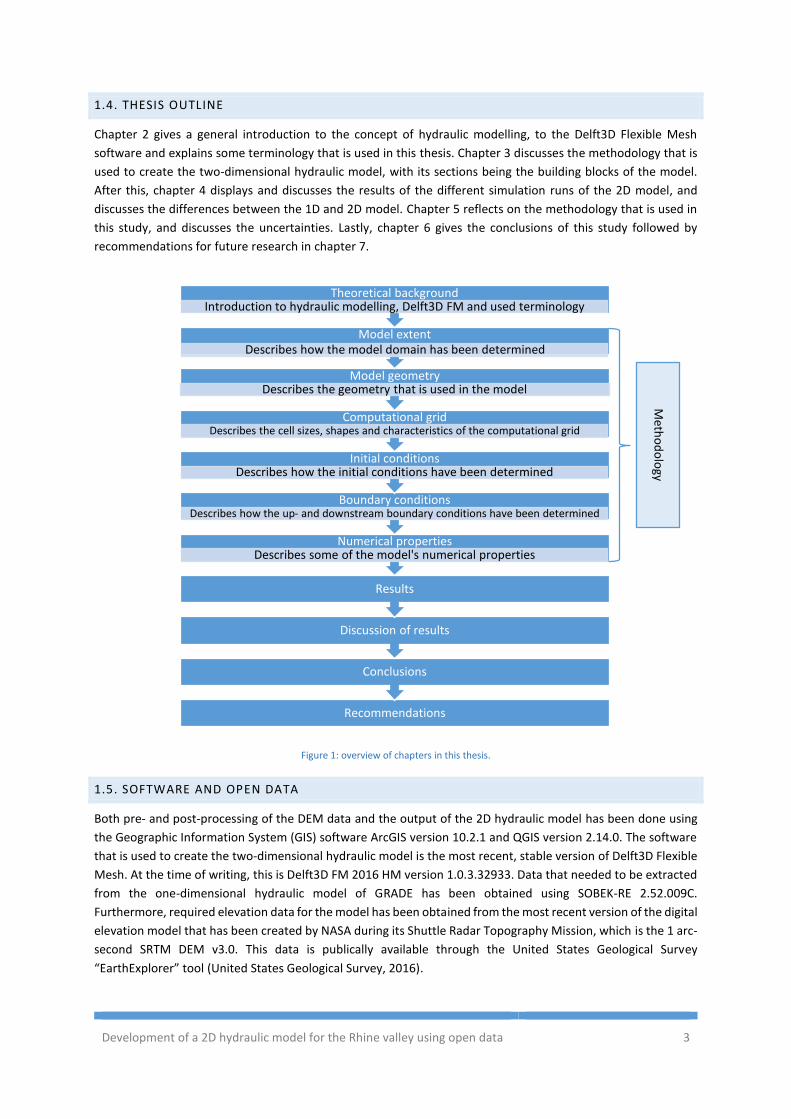
1.4. THESIS OUTLINE
Chapter 2 gives a general introduction to the concept of hydraulic modelling, to the Delft3D Flexible Mesh
software and explains some terminology that is used in this thesis. Chapter 3 discusses the methodology that is
used to create the two-dimensional hydraulic model, with its sections being the building blocks of the model.
After this, chapter 4 displays and discusses the results of the different simulation runs of the 2D model, and
discusses the differences between the 1D and 2D model. Chapter 5 reflects on the methodology that is used in
this study, and discusses the uncertainties. Lastly, chapter 6 gives the conclusions of this study followed by
recommendations for future research in chapter 7.
Figure 1: overview of chapters in this thesis.
1.5. SOFTWARE AND OPEN DATA
Both pre- and post-processing of the DEM data and the output of the 2D hydraulic model has been done using
the Geographic Information System (GIS) software ArcGIS version 10.2.1 and QGIS version 2.14.0. The software
that is used to create the two-dimensional hydraulic model is the most recent, stable version of Delft3D Flexible
Mesh. At the time of writing, this is Delft3D FM 2016 HM version 1.0.3.32933. Data that needed to be extracted
from the one-dimensional hydraulic model of GRADE has been obtained using SOBEK-RE 2.52.009C.
Furthermore, required elevation data for the model has been obtained from the most recent version of the digital
elevation model that has been created by NASA during its Shuttle Radar Topography Mission, which is the 1 arc-
second SRTM DEM v3.0. This data is publically available through the United States Geological Survey
“EarthExplorer” tool (United States Geological Survey, 2016).
Recommendations
Conclusions
Discussion of results
Results
Numerical propertiesDescribes some of the model's numerical properties
Boundary conditionsDescribes how the up- and downstream boundary conditions have been determined
Initial conditionsDescribes how the initial conditions have been determined
Computational gridDescribes the cell sizes, shapes and characteristics of the computational grid
Model geometryDescribes the geometry that is used in the model
Model extentDescribes how the model domain has been determined
Theoretical backgroundIntroduction to hydraulic modelling, Delft3D FM and used terminology
Meth
od
olo
gy
BSc Thesis – Martijn Kriebel 4
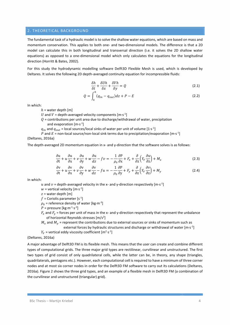
2. THEORETICAL BACKGROUND
The fundamental task of a hydraulic model is to solve the shallow water equations, which are based on mass and
momentum conservation. This applies to both one- and two-dimensional models. The difference is that a 2D
model can calculate this in both longitudinal and transversal direction (i.e. it solves the 2D shallow water
equations) as opposed to a one-dimensional model which only calculates the equations for the longitudinal
direction (Horritt & Bates, 2002).
For this study the hydrodynamic modelling software Delft3D Flexible Mesh is used, which is developed by
Deltares. It solves the following 2D depth-averaged continuity equation for incompressible fluids:
𝛿ℎ
𝛿𝑡+
𝛿𝑈ℎ
𝛿𝑥+
𝛿𝑉ℎ
𝛿𝑦= 𝑄 (2.1)
𝑄 = ∫ (𝑞𝑖𝑛 − 𝑞𝑜𝑢𝑡)𝑑𝑧 + 𝑃 − 𝐸ℎ
0
(2.2)
In which: ℎ = water depth [m] 𝑈 and 𝑉 = depth-averaged velocity components [m·s-1]
𝑄 = contributions per unit area due to discharge/withdrawal of water, precipitation and evaporation [m·s-1] 𝑞𝑖𝑛 and 𝑞𝑜𝑢𝑡 = local sources/local sinks of water per unit of volume [1·s-1] 𝑃 and 𝐸 = non-local source/non-local sink terms due to precipitation/evaporation [m·s-1]
(Deltares, 2016a)
The depth-averaged 2D momentum equation in x- and y-direction that the software solves is as follows:
∂u
∂t+ 𝑢
∂u
∂x+ 𝑣
∂u
∂y+ 𝑤
∂u
𝑑𝑧− 𝑓𝑣 = −
1
𝜌0
∂P
∂x+ 𝐹𝑥 +
∂
∂z(𝛶𝑉
∂u
∂z) + 𝑀𝑥 (2.3)
∂v
∂t+ 𝑢
∂v
∂x+ 𝑣
∂v
∂y+ 𝑤
∂v
𝑑𝑧− 𝑓𝑢 = −
1
𝜌0
∂P
∂y+ 𝐹𝑦 +
∂
∂z(𝛶𝑉
∂v
∂z) + 𝑀𝑦 (2.4)
In which: 𝑢 and 𝑣 = depth-averaged velocity in the x- and y-direction respectively [m·s-1] 𝑤 = vertical velocity [m·s-1] 𝑧 = water depth [m] 𝑓 = Coriolis parameter [s-1] 𝜌0 = reference density of water [kg·m-3] 𝑃 = pressure [kg·m-1·s-2]
𝐹𝑥 and 𝐹𝑦 = forces per unit of mass in the x- and y-direction respectively that represent the unbalance
of horizontal Reynolds stresses [m/s2] 𝑀𝑥 and 𝑀𝑦 = represent the contributions due to external sources or sinks of momentum such as
external forces by hydraulic structures and discharge or withdrawal of water [m·s-2] 𝛶𝑉 = vertical eddy viscosity coefficient [m2·s-1]
(Deltares, 2016a)
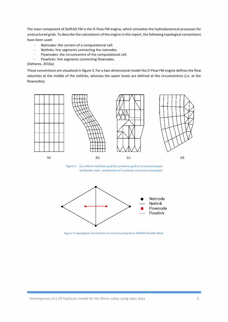
A major advantage of Delft3D FM is its flexible mesh. This means that the user can create and combine different
types of computational grids. The three major grid types are rectilinear, curvilinear and unstructured. The first
two types of grid consist of only quadrilateral cells, while the latter can be, in theory, any shape (triangles,
quadrilaterals, pentagons etc.). However, each computational cell is required to have a minimum of three corner
nodes and at most six corner nodes in order for the Delft3D FM software to carry out its calculations (Deltares,
2016a). Figure 2 shows the three grid types, and an example of a flexible mesh in Delft3D FM (a combination of
the curvilinear and unstructured (triangular) grid).
Development of a 2D hydraulic model for the Rhine valley using open data 5
The main component of Delft3D FM is the D-Flow FM engine, which simulates the hydrodynamical processes for
unstructured grids. To describe the calculations of the engine in this report, the following topological conventions
have been used:
- Netnodes: the corners of a computational cell. - Netlinks: line segments connecting the netnodes. - Flownodes: the circumcentre of the computational cell. - Flowlinks: line segments connecting flownodes.
(Deltares, 2016a)
These conventions are visualized in figure 3. For a two-dimensional model the D-Flow FM engine defines the flow
velocities at the middle of the netlinks, whereas the water levels are defined at the circumcentres (i.e. at the
flownodes).
Figure 2: (a) uniform rectilinear grid (b) curvilinear grid (c) unstructured grid
(d) flexible mesh: combination of curvilinear and unstructured grid
Figure 3: topological conventions of unstructured grids in Delft3D Flexible Mesh.
BSc Thesis – Martijn Kriebel 6
3. METHODOLOGY
3.1. MODEL EXTENT
An important, basic aspect regarding the development of a hydraulic model is the size of the domain that should
be taken into account (the model extent). One can decide to only include, for example, the Rhine with a buffer
of 50 meter around it. Although this model would require relatively few grid cells (and will consequently have a
low computation time), it is likely that in reality, the water will exceed the model domain in the case of an
extreme event. On the other hand, choosing a very large domain such as the Rhine with a buffer of 50 kilometer
results in many (unnecessary) grid cells and a higher computation time. Therefore, the model domain should be
made as large as the (maximum expected) spatial extent of the flooding during an extreme event.
In this methodology section an estimation of the minimum required domain is given. The process of defining this
domain consists of two major parts: estimating the probable extent of flooding of the river’s floodplains that
could occur in the case of an extreme discharge event, and estimating to what extent the tributaries should be
taken into account by looking at the backwater effect. When combined, an indication of the minimum required
domain is obtained.
3.1.1. FLOODPLAINS
Before looking at the possible floodplains in the case of an extreme discharge event, it is good to define the term
“floodplain” first. Loucks and van Beek (2005) define two types of floodplains: a hydrological floodplain, which is
inundated about two years out of three, and a topographic floodplain that is flooded by a flood peak of a given
frequency. The goal of the two-dimensional hydraulic model is to simulate extreme high discharges with high
return periods. Hegnauer, Kwadijk and Klijn (2015) estimate that the maximum plausible flood wave that can
arrive at Lobith has a discharge of 18 000 m3/s, with a corresponding return period of 100 000 years. Higher
discharges cannot be conveyed by the Niederrhein without embankment overtopping. In that case, the water
will enter the Netherlands over land and flows into e.g. the IJssel valley. However, it is likely that this will already
happen for lower discharges, since a discharge capacity of 18 000 m3/s in the Niederrhein is considered to be a
very high upper end estimation. This means that this scenario with a return period of 100 000 years can be used
as an indication of the maximal floodplain extent in the Rhine valley. Therefore, whenever the word “floodplain”
is used in this report, the topographic floodplain for an extreme discharge event with a return period of 100 000
years is meant.
The method that is used to get an indication of flooding of these floodplains can be summarized as follows:
1. The river is divided into sections, based on the slope. This slope should be roughly linear per section.
2. Using a modified version of the Chézy equation and known river properties the water level that occurs
during an extreme discharge event can be estimated.
3. These water levels have been linearly interpolated over all the other river cells.
4. The water levels of all the points on the river are interpolated over the DEM using the inverse distance
weighting method, and all the DEM cells that are below the corresponding water level are marked as
“flooded”.
5. All the flooded DEM cells that are not connected to the Rhine are removed.
The first two steps have been performed manually, while the remaining steps have been executed by a
customized Python script. The output of this method is an overview of areas along the Rhine which are likely to
be inundated in the case of the extreme discharge event.
Development of a 2D hydraulic model for the Rhine valley using open data 7
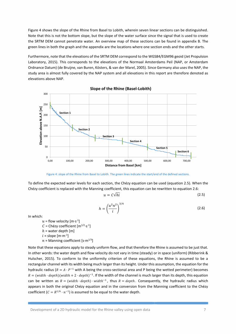
Figure 4 shows the slope of the Rhine from Basel to Lobith, wherein seven linear sections can be distinguished.
Note that this is not the bottom slope, but the slope of the water surface since the signal that is used to create
the SRTM DEM cannot penetrate water. An overview map of these sections can be found in appendix B. The
green lines in both the graph and the appendix are the locations where one section ends and the other starts.
Furthermore, note that the elevations of the SRTM DEM correspond to the WGS84/EGM96 geoid (Jet Propulsion
Laboratory, 2015). This corresponds to the elevations of the Normaal Amsterdams Peil (NAP, or Amsterdam
Ordnance Datum) (de Bruijne, van Buren, Kösters, & van der Marel, 2005). Since Germany also uses the NAP, the
study area is almost fully covered by the NAP system and all elevations in this report are therefore denoted as
elevations above NAP.
Figure 4: slope of the Rhine from Basel to Lobith. The green lines indicate the start/end of the defined sections.
To define the expected water levels for each section, the Chézy equation can be used (equation 2.5). When the
Chézy coefficient is replaced with the Manning coefficient, this equation can be rewritten to equation 2.6:
𝑢 = 𝐶√ℎ𝑖 (2.5)
ℎ = (𝑢2𝑛2
𝑖)
3/4
(2.6)
In which: 𝑢 = flow velocity [m·s-1] 𝐶 = Chézy coefficient [m1/2·s-1] ℎ = water depth [m] 𝑖 = slope [m·m-1] 𝑛 = Manning coefficient [s·m1/3]
Note that these equations apply to steady uniform flow, and that therefore the Rhine is assumed to be just that.
In other words: the water depth and flow velocity do not vary in time (steady) or in space (uniform) (Ribberink &
Hulscher, 2015). To conform to the uniformity criterion of these equations, the Rhine is assumed to be a
rectangular channel with its width being much larger than its height. Under this assumption, the equation for the
hydraulic radius (𝑅 = 𝐴 · 𝑃−1 with A being the cross-sectional area and P being the wetted perimeter) becomes
𝑅 = (𝑤𝑖𝑑𝑡ℎ · 𝑑𝑒𝑝𝑡ℎ)(𝑤𝑖𝑑𝑡ℎ + 2 · 𝑑𝑒𝑝𝑡ℎ)−1. If the width of the channel is much larger than its depth, this equation
can be written as 𝑅 = (𝑤𝑖𝑑𝑡ℎ · 𝑑𝑒𝑝𝑡ℎ) · 𝑤𝑖𝑑𝑡ℎ−1 , thus 𝑅 = 𝑑𝑒𝑝𝑡ℎ . Consequently, the hydraulic radius which
appears in both the original Chézy equation and in the conversion from the Manning coefficient to the Chézy
coefficient (𝐶 = 𝑅1/6 · 𝑛−1) is assumed to be equal to the water depth.
0
50
100
150
200
250
300
0,00 100,00 200,00 300,00 400,00 500,00 600,00 700,00
Elev
atio
n a
bo
ve N
.A.P
. [m
]
Distance from Basel [km]
Slope of the Rhine (Basel-Lobith)
Section 1
Section 2
Section 3
Section 4
Section 5Section 6
BSc Thesis – Martijn Kriebel 8
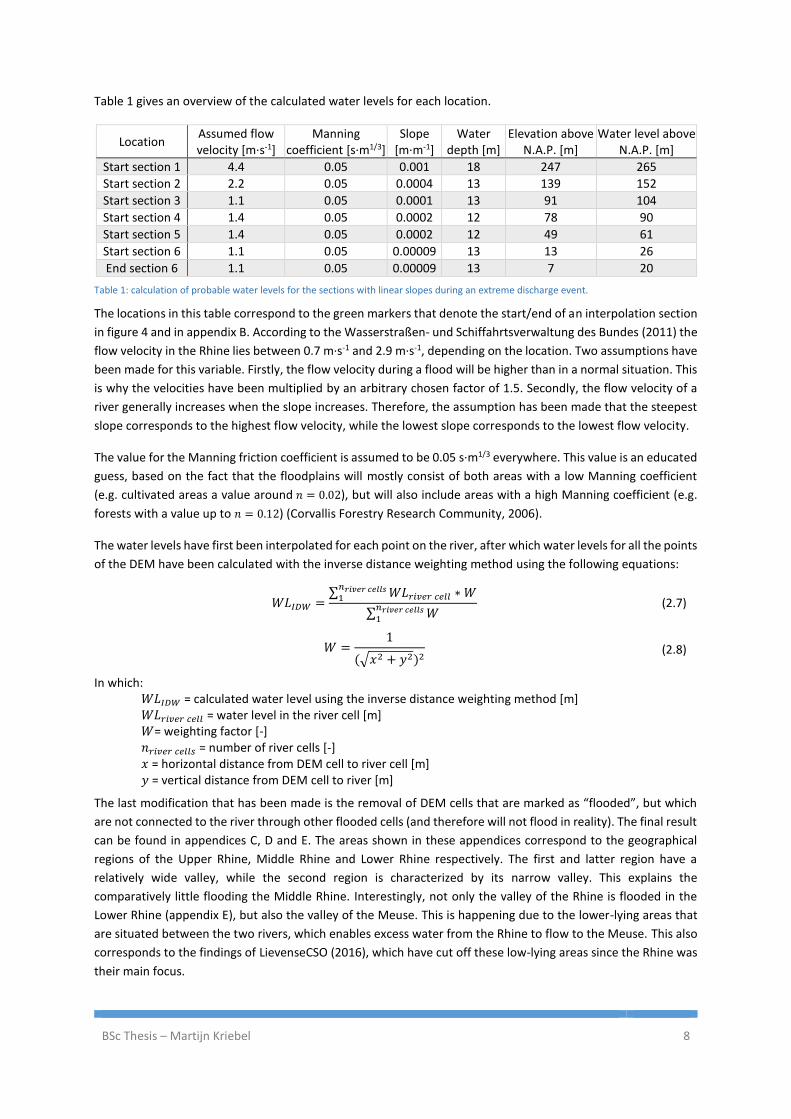
Table 1 gives an overview of the calculated water levels for each location.
Location Assumed flow velocity [m·s-1]
Manning coefficient [s·m1/3]
Slope [m·m-1]
Water depth [m]
Elevation above N.A.P. [m]
Water level above N.A.P. [m]
Start section 1 4.4 0.05 0.001 18 247 265
Start section 2 2.2 0.05 0.0004 13 139 152
Start section 3 1.1 0.05 0.0001 13 91 104
Start section 4 1.4 0.05 0.0002 12 78 90
Start section 5 1.4 0.05 0.0002 12 49 61
Start section 6 1.1 0.05 0.00009 13 13 26
End section 6 1.1 0.05 0.00009 13 7 20
Table 1: calculation of probable water levels for the sections with linear slopes during an extreme discharge event.
The locations in this table correspond to the green markers that denote the start/end of an interpolation section
in figure 4 and in appendix B. According to the Wasserstraßen- und Schiffahrtsverwaltung des Bundes (2011) the
flow velocity in the Rhine lies between 0.7 m·s-1 and 2.9 m·s-1, depending on the location. Two assumptions have
been made for this variable. Firstly, the flow velocity during a flood will be higher than in a normal situation. This
is why the velocities have been multiplied by an arbitrary chosen factor of 1.5. Secondly, the flow velocity of a
river generally increases when the slope increases. Therefore, the assumption has been made that the steepest
slope corresponds to the highest flow velocity, while the lowest slope corresponds to the lowest flow velocity.
The value for the Manning friction coefficient is assumed to be 0.05 s·m1/3 everywhere. This value is an educated
guess, based on the fact that the floodplains will mostly consist of both areas with a low Manning coefficient
(e.g. cultivated areas a value around 𝑛 = 0.02), but will also include areas with a high Manning coefficient (e.g.
forests with a value up to 𝑛 = 0.12) (Corvallis Forestry Research Community, 2006).
The water levels have first been interpolated for each point on the river, after which water levels for all the points
of the DEM have been calculated with the inverse distance weighting method using the following equations:
𝑊𝐿𝐼𝐷𝑊 =∑ 𝑊𝐿𝑟𝑖𝑣𝑒𝑟 𝑐𝑒𝑙𝑙 ∗ 𝑊
𝑛𝑟𝑖𝑣𝑒𝑟 𝑐𝑒𝑙𝑙𝑠1
∑ 𝑊𝑛𝑟𝑖𝑣𝑒𝑟 𝑐𝑒𝑙𝑙𝑠1
(2.7)
𝑊 =1
(√𝑥2 + 𝑦2)2 (2.8)
In which: 𝑊𝐿𝐼𝐷𝑊 = calculated water level using the inverse distance weighting method [m] 𝑊𝐿𝑟𝑖𝑣𝑒𝑟 𝑐𝑒𝑙𝑙 = water level in the river cell [m] 𝑊= weighting factor [-] 𝑛𝑟𝑖𝑣𝑒𝑟 𝑐𝑒𝑙𝑙𝑠 = number of river cells [-] 𝑥 = horizontal distance from DEM cell to river cell [m] 𝑦 = vertical distance from DEM cell to river [m]
The last modification that has been made is the removal of DEM cells that are marked as “flooded”, but which
are not connected to the river through other flooded cells (and therefore will not flood in reality). The final result
can be found in appendices C, D and E. The areas shown in these appendices correspond to the geographical
regions of the Upper Rhine, Middle Rhine and Lower Rhine respectively. The first and latter region have a
relatively wide valley, while the second region is characterized by its narrow valley. This explains the
comparatively little flooding the Middle Rhine. Interestingly, not only the valley of the Rhine is flooded in the
Lower Rhine (appendix E), but also the valley of the Meuse. This is happening due to the lower-lying areas that
are situated between the two rivers, which enables excess water from the Rhine to flow to the Meuse. This also
corresponds to the findings of LievenseCSO (2016), which have cut off these low-lying areas since the Rhine was
their main focus.
Development of a 2D hydraulic model for the Rhine valley using open data 9
3.1.2. TRIBUTARY BACKWATER
Appendices C, D and E include flooding that could occur at the lower parts of the tributaries of the Rhine.
However, the extent to which the valleys of the tributaries would flood will be less in reality since the method
from the previous paragraph only takes the effects of the water from the Rhine into account, and not the
opposing force of the water from the tributaries. Besides this, the tributaries are often situated perpendicular to
the flow direction in the Rhine, making it hard for the water to enter the tributary. To get a better idea how much
of the tributaries should be included in the model, one can look at the backwater adaptation length.
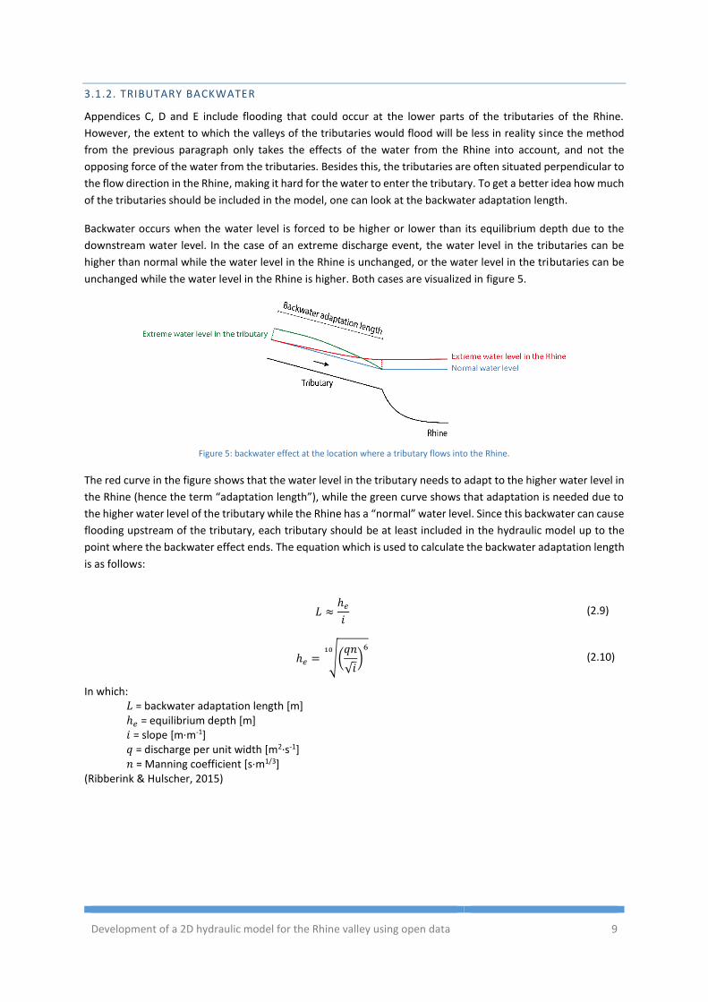
Backwater occurs when the water level is forced to be higher or lower than its equilibrium depth due to the
downstream water level. In the case of an extreme discharge event, the water level in the tributaries can be
higher than normal while the water level in the Rhine is unchanged, or the water level in the tributaries can be
unchanged while the water level in the Rhine is higher. Both cases are visualized in figure 5.
Figure 5: backwater effect at the location where a tributary flows into the Rhine.
The red curve in the figure shows that the water level in the tributary needs to adapt to the higher water level in
the Rhine (hence the term “adaptation length”), while the green curve shows that adaptation is needed due to
the higher water level of the tributary while the Rhine has a “normal” water level. Since this backwater can cause
flooding upstream of the tributary, each tributary should be at least included in the hydraulic model up to the
point where the backwater effect ends. The equation which is used to calculate the backwater adaptation length
is as follows:
𝐿 ≈ℎ𝑒
𝑖 (2.9)
ℎ𝑒 = √(𝑞𝑛
√𝑖)
610
(2.10)
In which: 𝐿 = backwater adaptation length [m] ℎ𝑒 = equilibrium depth [m] 𝑖 = slope [m·m-1] 𝑞 = discharge per unit width [m2·s-1] 𝑛 = Manning coefficient [s·m1/3]
(Ribberink & Hulscher, 2015)
BSc Thesis – Martijn Kriebel 10
Equation 2.9 is true for small values of the Froude number (Fr < 1, i.e. for subcritical flow). A flow is subcritical
when its slope is lower than the critical slope 𝑖𝑐:
𝑖𝑐 =𝑔𝑛2
√ℎ3 (2.11)
In which: 𝑖𝑐 = critical slope [m·m-1] 𝑔 = gravitational acceleration [m·s-2] 𝑛 = Manning coefficient [s·m1/3] ℎ = water depth [m]
(Ribberink & Hulscher, 2015)
Since the gravitational acceleration and the Manning coefficient in this equation are assumed to be constant
(𝑔 = 9.81 m·s-2 and 𝑛 = 0.05 s·m1/3), the critical slope can only be reached by varying the water depth, which is
calculated in table 1. These calculations result in the conclusion that all slopes are below the critical slope,
meaning that all flows are subcritical and equation 2.9 can be used.
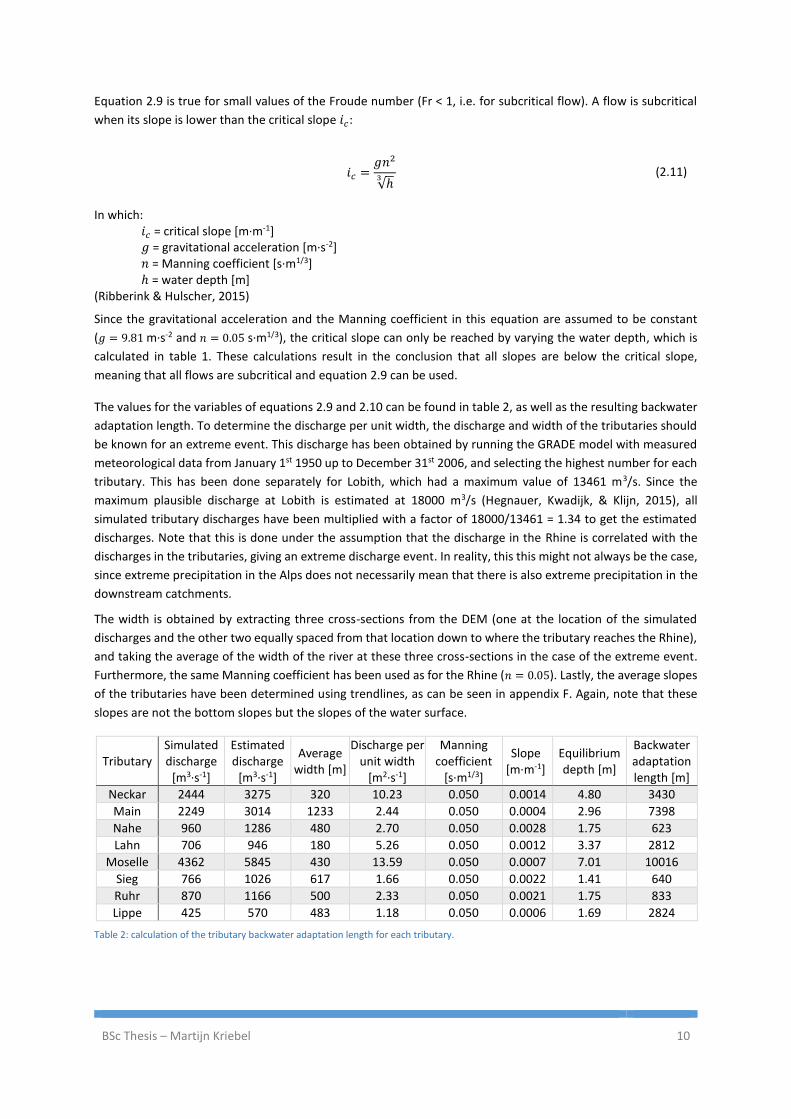
The values for the variables of equations 2.9 and 2.10 can be found in table 2, as well as the resulting backwater
adaptation length. To determine the discharge per unit width, the discharge and width of the tributaries should
be known for an extreme event. This discharge has been obtained by running the GRADE model with measured
meteorological data from January 1st 1950 up to December 31st 2006, and selecting the highest number for each
tributary. This has been done separately for Lobith, which had a maximum value of 13461 m3/s. Since the
maximum plausible discharge at Lobith is estimated at 18000 m3/s (Hegnauer, Kwadijk, & Klijn, 2015), all
simulated tributary discharges have been multiplied with a factor of 18000/13461 = 1.34 to get the estimated
discharges. Note that this is done under the assumption that the discharge in the Rhine is correlated with the
discharges in the tributaries, giving an extreme discharge event. In reality, this this might not always be the case,
since extreme precipitation in the Alps does not necessarily mean that there is also extreme precipitation in the
downstream catchments.
The width is obtained by extracting three cross-sections from the DEM (one at the location of the simulated
discharges and the other two equally spaced from that location down to where the tributary reaches the Rhine),
and taking the average of the width of the river at these three cross-sections in the case of the extreme event.
Furthermore, the same Manning coefficient has been used as for the Rhine (𝑛 = 0.05). Lastly, the average slopes
of the tributaries have been determined using trendlines, as can be seen in appendix F. Again, note that these
slopes are not the bottom slopes but the slopes of the water surface.
Tributary Simulated discharge
[m3·s-1]
Estimated discharge
[m3·s-1]
Average width [m]
Discharge per unit width
[m2·s-1]
Manning coefficient
[s·m1/3]
Slope [m·m-1]
Equilibrium depth [m]
Backwater adaptation length [m]
Neckar 2444 3275 320 10.23 0.050 0.0014 4.80 3430
Main 2249 3014 1233 2.44 0.050 0.0004 2.96 7398
Nahe 960 1286 480 2.70 0.050 0.0028 1.75 623
Lahn 706 946 180 5.26 0.050 0.0012 3.37 2812
Moselle 4362 5845 430 13.59 0.050 0.0007 7.01 10016
Sieg 766 1026 617 1.66 0.050 0.0022 1.41 640
Ruhr 870 1166 500 2.33 0.050 0.0021 1.75 833
Lippe 425 570 483 1.18 0.050 0.0006 1.69 2824
Table 2: calculation of the tributary backwater adaptation length for each tributary.
Development of a 2D hydraulic model for the Rhine valley using open data 11
Overall, these backwater adaptation lengths just under or almost the same as the indicative floodplains which
have been determined in section 3.1.1.
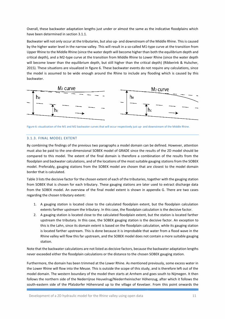
Backwater will not only occur at the tributaries, but also up- and downstream of the Middle Rhine. This is caused
by the higher water level in the narrow valley. This will result in a so-called M1-type curve at the transition from
Upper Rhine to the Middle Rhine (since the water depth will become higher than both the equilibrium depth and
critical depth), and a M2-type curve at the transition from Middle Rhine to Lower Rhine (since the water depth
will become lower than the equilibrium depth, but still higher than the critical depth) (Ribberink & Hulscher,
2015). These situations are visualized in figure 6. These backwater events do not require any calculations, since
the model is assumed to be wide enough around the Rhine to include any flooding which is caused by this
backwater.
Figure 6: visualization of the M1 and M2 backwater curves that will occur respectively just up- and downstream of the Middle Rhine.
3.1.3. FINAL MODEL EXTENT
By combining the findings of the previous two paragraphs a model domain can be defined. However, attention
must also be paid to the one-dimensional SOBEK model of GRADE since the results of the 2D model should be
compared to this model. The extent of the final domain is therefore a combination of the results from the
floodplain and backwater calculations, and of the locations of the most suitable gauging stations from the SOBEK
model. Preferably, gauging stations from the SOBEK model are chosen that are closest to the model domain
border that is calculated.
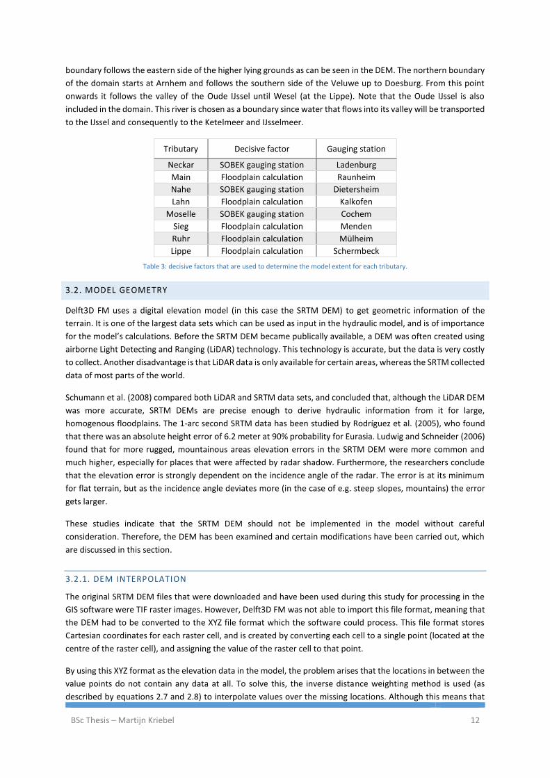
Table 3 lists the decisive factor for the chosen extent of each of the tributaries, together with the gauging station
from SOBEK that is chosen for each tributary. These gauging stations are later used to extract discharge data
from the SOBEK model. An overview of the final model extent is shown in appendix G. There are two cases
regarding the chosen tributary extent:
1. A gauging station is located close to the calculated floodplain extent, but the floodplain calculation
extents farther upstream the tributary. In this case, the floodplain calculation is the decisive factor.
2. A gauging station is located close to the calculated floodplain extent, but the station is located farther
upstream the tributary. In this case, the SOBEK gauging station is the decisive factor. An exception to
this is the Lahn, since its domain extent is based on the floodplain calculation, while its gauging station
is located farther upstream. This is done because it is improbable that water from a flood wave in the
Rhine valley will flow this far upstream, and the SOBEK model does not contain a more suitable gauging
station.
Note that the backwater calculations are not listed as decisive factors, because the backwater adaptation lengths
never exceeded either the floodplain calculations or the distance to the chosen SOBEK gauging station.
Furthermore, the domain has been trimmed at the Lower Rhine. As mentioned previously, some excess water in
the Lower Rhine will flow into the Meuse. This is outside the scope of this study, and is therefore left out of the
model domain. The western boundary of the model then starts at Arnhem and goes south to Nijmegen. It then
follows the northern side of the Nederrijnse Heuvelrug/Niederrheinischer Höhenzug, after which it follows the
south-eastern side of the Pfalzdorfer Höhenrand up to the village of Kevelaer. From this point onwards the
BSc Thesis – Martijn Kriebel 12
boundary follows the eastern side of the higher lying grounds as can be seen in the DEM. The northern boundary
of the domain starts at Arnhem and follows the southern side of the Veluwe up to Doesburg. From this point
onwards it follows the valley of the Oude IJssel until Wesel (at the Lippe). Note that the Oude IJssel is also
included in the domain. This river is chosen as a boundary since water that flows into its valley will be transported
to the IJssel and consequently to the Ketelmeer and IJsselmeer.
Tributary Decisive factor Gauging station
Neckar SOBEK gauging station Ladenburg
Main Floodplain calculation Raunheim
Nahe SOBEK gauging station Dietersheim
Lahn Floodplain calculation Kalkofen
Moselle SOBEK gauging station Cochem
Sieg Floodplain calculation Menden
Ruhr Floodplain calculation Mülheim
Lippe Floodplain calculation Schermbeck
Table 3: decisive factors that are used to determine the model extent for each tributary.
3.2. MODEL GEOMETRY
Delft3D FM uses a digital elevation model (in this case the SRTM DEM) to get geometric information of the
terrain. It is one of the largest data sets which can be used as input in the hydraulic model, and is of importance
for the model’s calculations. Before the SRTM DEM became publically available, a DEM was often created using
airborne Light Detecting and Ranging (LiDAR) technology. This technology is accurate, but the data is very costly
to collect. Another disadvantage is that LiDAR data is only available for certain areas, whereas the SRTM collected
data of most parts of the world.
Schumann et al. (2008) compared both LiDAR and SRTM data sets, and concluded that, although the LiDAR DEM
was more accurate, SRTM DEMs are precise enough to derive hydraulic information from it for large,
homogenous floodplains. The 1-arc second SRTM data has been studied by Rodríguez et al. (2005), who found
that there was an absolute height error of 6.2 meter at 90% probability for Eurasia. Ludwig and Schneider (2006)
found that for more rugged, mountainous areas elevation errors in the SRTM DEM were more common and
much higher, especially for places that were affected by radar shadow. Furthermore, the researchers conclude
that the elevation error is strongly dependent on the incidence angle of the radar. The error is at its minimum
for flat terrain, but as the incidence angle deviates more (in the case of e.g. steep slopes, mountains) the error
gets larger.
These studies indicate that the SRTM DEM should not be implemented in the model without careful
consideration. Therefore, the DEM has been examined and certain modifications have been carried out, which
are discussed in this section.
3.2.1. DEM INTERPOLATION
The original SRTM DEM files that were downloaded and have been used during this study for processing in the
GIS software were TIF raster images. However, Delft3D FM was not able to import this file format, meaning that
the DEM had to be converted to the XYZ file format which the software could process. This file format stores
Cartesian coordinates for each raster cell, and is created by converting each cell to a single point (located at the
centre of the raster cell), and assigning the value of the raster cell to that point.
By using this XYZ format as the elevation data in the model, the problem arises that the locations in between the
value points do not contain any data at all. To solve this, the inverse distance weighting method is used (as
described by equations 2.7 and 2.8) to interpolate values over the missing locations. Although this means that
Development of a 2D hydraulic model for the Rhine valley using open data 13
the model does not use the original raster DEM, this modification makes sure that elevation changes occur
gradually instead of abruptly, making the DEM more realistic.
Another modification which involves interpolation concerns the tributaries. These are all relatively narrow, which
causes misrepresentation of the elevations of the tributaries in the DEM. As a consequence, the tributary
elevation increases when going downstream in some cases, which is not realistic. To solve this, the elevation has
been linearly interpolated between the model boundary at that tributary and the location where the tributary
meets the Rhine. Note that none of the models include actual tributary bathymetry. Rather, smoothing of the
DEM (i.e. the water surface) is carried out.
3.2.2. BATHYMETRY
Another modification that is carried out on the DEM is the incorporation of the bathymetry of the Rhine. Since
the hydraulic model is initially a basic model, basic bathymetry is used. This means that the Rhine is assumed to
be a rectangular channel that has a constant depth along its length. This bathymetry needs to be “burned” into
the DEM, since it does not include elevations below the water surface. It is assumed that the channel depth is
equal to the initial water depth in the Rhine (which is 3 meter, as described in chapter 3.4). This means that at
the location of the main channel the DEM cells have been lowered by 3 meter. Note that this is an overestimation,
since the mean water depth will, in reality, most likely not result in a completely filled channel. Also, since this
channel depth is an average, it is an overestimation at some areas (mostly upstream) and an underestimation at
other locations (mostly downstream).
The part of the Upper Rhine where the Great Alsace Canal is located is a special case. Here, most of the water is
located in the Great Alsace canal, while the “actual” Rhine conveys less water (which is supported by the DEM,
since values at this part of the Rhine are lower than in the Great Alsace canal). This is done so that the
hydroelectric power stations at Kembs, Ottmarsheim, Fessenheim and Vogelgrün are provided with enough
water (Becker, Schwanenberg, Hatz, & Schruff, 2012). However, satellite pictures show that there is still water
located in the “actual” Rhine. Therefore, 3-meter-deep bathymetry is burnt at both locations. Note that this is
most certainly an overestimation, and that this should be changed if more detailed information is obtained.
Note that none of the models include tributary bathymetry, as mentioned in the previous section.
3.3. COMPUTATIONAL GRID
This methodology section describes the process of how the computational grid has been created. As explained
in chapter 2 a hydraulic model solves continuity and mass equations. However, this cannot simply be done for
the full model domain at once. Instead, the domain should be divided into several volume elements:
computational cells (Loucks & van Beek, 2005). The model then solves the continuity and mass equations for
each cell, resulting in detailed output. All the computational cells combined form the computational grid.
Bates and De Roo (2000) studied the possible grid cell sizes as they propose a simple raster-based (2D) flood
inundation model. As expected, smaller cells give the most accurate result in both studies. However, smaller grid
cells have some drawbacks. One of those is that it increases the required computation time significantly. This
corresponds to the findings of Werner (2000) on his DEM based 1D model.
A second drawback of small grid cell sizes is that it makes a model more complex, and thus more complicated for
the user. Bates and De Roo (2000) state that simpler models would be beneficial, as they could ideally be used
by people with little hydraulic modelling experience. According to them, the best model would be the simplest
one that provides the information that is needed by the user, whilst reasonably fitting the available data. This
corresponds to the well-known problem-solving principle of Occam’s razor, which says that no more assumptions
BSc Thesis – Martijn Kriebel 14
should be made than the minimum that is required. The best grid cell size is therefore the one which balances
accuracy and computation time best (i.e. the most optimal grid cell size).
Another characteristic that can influence the performance of a model, the shape of the computational cells. If,
for example, a rectilinear grid would be laid over of the area of interest, troubles can arise at parts where the
river is highly sinuous. If interpolation of cross-sections is needed to obtain the bathymetry at that location, the
model would give wrong results since it assumes the river to be continually straight instead of sinuous (Merwade,
Cook, & Coonrod, 2008). Of course, this can be solved in the Delft3D FM software by creating a curvilinear grid
that follows the curves of the river. The creation and application of this grid together with other types are
described in the following subsections.
3.3.1. MAIN CHANNEL AND FLOODPLAIN GRID
Two major parts of the computational grid can be distinguished: the main channel grid and the floodplain grid.
This is easy to see since the main channel grid is curvilinear, while the floodplain grid is unstructured. Despite
these differences, they form one integral grid because of the flexible mesh feature of Delft3D FM.
The main reason for a curvilinear grid at the Rhine is because it is computationally less intensive compared to an
unstructured grid. A straight part of the river can easily be covered by one curvilinear cell, since it is unlikely that
variables like water depth and velocity will change much there. When this part would be covered by unstructured
cells, much more cells would be needed, thus increasing the required computation time.
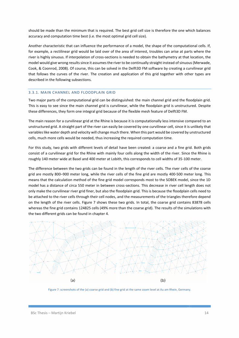
For this study, two grids with different levels of detail have been created: a coarse and a fine grid. Both grids
consist of a curvilinear grid for the Rhine with mainly four cells along the width of the river. Since the Rhine is
roughly 140 meter wide at Basel and 400 meter at Lobith, this corresponds to cell widths of 35-100 meter.
The difference between the two grids can be found in the length of the river cells. The river cells of the coarse
grid are mostly 800–900 meter long, while the river cells of the fine grid are mostly 400-500 meter long. This
means that the calculation method of the fine grid model corresponds most to the SOBEK model, since the 1D
model has a distance of circa 550 meter in between cross-sections. This decrease in river cell length does not
only make the curvilinear river grid finer, but also the floodplain grid. This is because the floodplain cells need to
be attached to the river cells through their cell nodes, and the measurements of the triangles therefore depend
on the length of the river cells. Figure 7 shows these two grids. In total, the coarse grid contains 83878 cells
whereas the fine grid contains 124825 cells (49% more than the coarse grid). The results of the simulations with
the two different grids can be found in chapter 4.
Figure 7: screenshots of the (a) coarse grid and (b) fine grid at the same zoom level at Au am Rhein, Germany.
Development of a 2D hydraulic model for the Rhine valley using open data 15
3.3.2. TRIBUTARY GRID
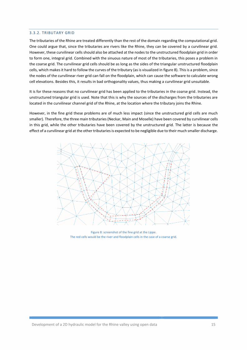
The tributaries of the Rhine are treated differently than the rest of the domain regarding the computational grid.
One could argue that, since the tributaries are rivers like the Rhine, they can be covered by a curvilinear grid.
However, these curvilinear cells should also be attached at the nodes to the unstructured floodplain grid in order
to form one, integral grid. Combined with the sinuous nature of most of the tributaries, this poses a problem in
the coarse grid. The curvilinear grid cells should be as long as the sides of the triangular unstructured floodplain
cells, which makes it hard to follow the curves of the tributary (as is visualized in figure 8). This is a problem, since
the nodes of the curvilinear river grid can fall on the floodplain, which can cause the software to calculate wrong
cell elevations. Besides this, it results in bad orthogonality values, thus making a curvilinear grid unsuitable.
It is for these reasons that no curvilinear grid has been applied to the tributaries in the coarse grid. Instead, the
unstructured triangular grid is used. Note that this is why the sources of the discharges from the tributaries are
located in the curvilinear channel grid of the Rhine, at the location where the tributary joins the Rhine.
However, in the fine grid these problems are of much less impact (since the unstructured grid cells are much
smaller). Therefore, the three main tributaries (Neckar, Main and Moselle) have been covered by curvilinear cells
in this grid, while the other tributaries have been covered by the unstructured grid. The latter is because the
effect of a curvilinear grid at the other tributaries is expected to be negligible due to their much smaller discharge.
Figure 8: screenshot of the fine grid at the Lippe.
The red cells would be the river and floodplain cells in the case of a coarse grid.
BSc Thesis – Martijn Kriebel 16
3.3.3. IRREGULARITIES
The Rhine contains some irregularities, especially in the Upper Rhine. One of the biggest irregularities is caused
by the Grand Canal d’Alsace (Great Alsace Canal). This canal is 50 kilometer long and runs parallel to the Rhine,
starting just downstream of Basel and ending at Breisach am Rhein (Germany). Because of this, a large island is
formed which is bounded by the Rhine and the channel. Furthermore, significant islands can be found at:
- Marckolsheim - Schoenau (the Réserve Naturelle de l’Île de Rhinau) - Schwanau - Strasbourg (the Réserve Naturelle de l’Île du Rohrschollen) - Rheinau - Iffezheim - Between Mainz and Bingen am Rhein (This area contains multiple islands, and if therefore also called
the Inselrhein, or “island Rhine”) - Lorch (the Lorcher Werth) - Niederwerth (including the Graswerth island) - Weißenthurm (the Weißenthurmer Werth)
Some of these islands are formed naturally, while others are river locks or hydroelectric power plants (note that
the effect of the constructions themselves are not taken into account in the model).
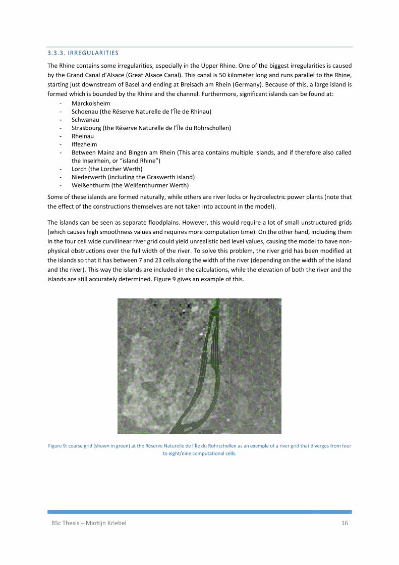
The islands can be seen as separate floodplains. However, this would require a lot of small unstructured grids
(which causes high smoothness values and requires more computation time). On the other hand, including them
in the four cell wide curvilinear river grid could yield unrealistic bed level values, causing the model to have non-
physical obstructions over the full width of the river. To solve this problem, the river grid has been modified at
the islands so that it has between 7 and 23 cells along the width of the river (depending on the width of the island
and the river). This way the islands are included in the calculations, while the elevation of both the river and the
islands are still accurately determined. Figure 9 gives an example of this.
Figure 9: coarse grid (shown in green) at the Réserve Naturelle de l’Île du Rohrschollen as an example of a river grid that diverges from four
to eight/nine computational cells.
Development of a 2D hydraulic model for the Rhine valley using open data 17
3.3.4. GRID CHARACTERISTICS
Two important properties of the computational grid are the orthogonality and the smoothness. The
orthogonality is defined as the cosine of the angle between a flowlink and a netlink. The smoothness is defined
as the ratio of the areas of two adjacent cells (Deltares, 2016a). In an ideal situation the orthogonality is 0 (i.e.
the angle between the flow- and netlink is 90°), while the smoothness is equal to 1. If a grid is orthogonal,
computationally expensive transformation terms do not have to be executed, which saves computation time.
Furthermore, a smooth grid minimizes the errors in the finite difference approximations (Deltares, 2016b).
However, it is hard to create a perfect grid in reality. Therefore, an orthogonality of 0.01 or lower is also
acceptable (Deltares, 2016a). Furthermore, experience shows that a smoothness of between 1-1.2 is sufficient
(Anke Becker, personal communication, May 17, 2016).
The orthogonality and smoothness of both the coarse and fine grid are shown in appendices H, I, J and K. It is
clear that the majority of the cells of all four pictures are dark blue. This means that most cells have an
orthogonality between 0 and 0.042, and a smoothness between 1 and 2.350. Closer examination of the grid show
that the majority of the cells has orthogonality and smoothness values that correspond to the advised values.
Slightly higher values can be found where the grid of the river is attached to the grid of the floodplain. The higher
orthogonality values can be explained by the curves of the rivers. Higher values for the smoothness at those
locations occur because the triangular cells are almost always larger than the river cells. The legends of the figures
show also much higher values. These cells are not immediately visible in the figures. They are all single cells which
are simply positioned in an unfortunate way. The effects of these cells can be neglected compared to the total
amount of cells.
3.3.5. FINAL GRID
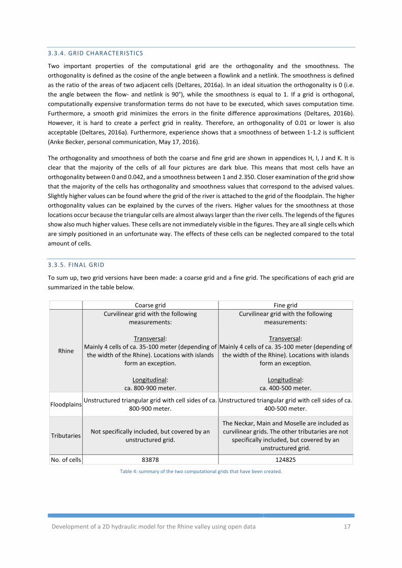
To sum up, two grid versions have been made: a coarse grid and a fine grid. The specifications of each grid are
summarized in the table below.
Table 4: summary of the two computational grids that have been created.
Coarse grid Fine grid
Rhine
Curvilinear grid with the following measurements:
Transversal:
Mainly 4 cells of ca. 35-100 meter (depending of the width of the Rhine). Locations with islands
form an exception.
Longitudinal: ca. 800-900 meter.
Curvilinear grid with the following measurements:
Transversal:
Mainly 4 cells of ca. 35-100 meter (depending of the width of the Rhine). Locations with islands
form an exception.
Longitudinal: ca. 400-500 meter.
Floodplains Unstructured triangular grid with cell sides of ca.
800-900 meter. Unstructured triangular grid with cell sides of ca.
400-500 meter.
Tributaries Not specifically included, but covered by an
unstructured grid.
The Neckar, Main and Moselle are included as curvilinear grids. The other tributaries are not
specifically included, but covered by an unstructured grid.
No. of cells 83878 124825
BSc Thesis – Martijn Kriebel 18
3.4. INITIAL CONDITIONS
Before a model can be run, initial conditions need to be specified which are used by the model as a starting point.
These initial conditions are water surface elevation and flow velocity (Maddock, Harby, Kemp, & Wood, 2013).
There are two possibilities for specifying these conditions: a cold start and a hot start. A cold start means that
the conditions are simply estimated. When applying a hot start, these elevations are specified from either
previous simulations or from measurements. The cold start method is the most common, since flood waves are
mostly the results from the inflows that are specified in the hydrographs. If a sufficiently long warm-up time is
being applied when using a cold start, the simulated flood wave will not have been influenced much by the initial
conditions (Engineers Australia, 2012).
For the Rhine, the average water depths at its major gauging stations over a period of ten years have been
collected and averaged. These average water depths can be found in appendix L. As a result, the initial water
depth in the Rhine has been set to 3 meter. To get the initial water surface elevation one simply adds this value
to the elevation of corresponding DEM cell in the main channel. As mentioned in chapter 3.2.2, the part of the
Upper Rhine where the Great Alsace Canal is located is a special case. Here, all the water is assumed to be located
in the Great Alsace canal, while the “actual” Rhine is assumed to be empty. Also note that the 3 meter channel
depth is an overestimation at some areas (mostly upstream) and an underestimation at other locations (mostly
downstream).
An initial condition that is used in the one-dimensional SOBEK model is initial discharge. This discharge is specified
for each of the model’s branches, causing initial flow velocities. Although this is not possible in Delft3D FM, a so-
called restart file can be used which makes it possible to use the flow velocities of a previously run simulation in
a new simulation. This restart file also contains other variables like the initial water depth which is mentioned
above. However, to make an accurate comparison between the SOBEK and Delft3D FM model, the same initial
velocities should be used. The 1D model contains varying initial velocities since the initial discharges are varying
from 1440-2300 m3/s. This varying flow velocity field is more difficult to create Delft3D FM, since it is not possible
to set an initial discharge for each computational cell (while in SOBEK one can specify one initial discharge per
branch). In order to recreate the initial discharges of the 1D model as good as possible, initial flow velocities are
obtained from the steady state results of a 2D model (to prevent a warm-up period from occurring) with a
constant discharge of 1870 m3/s at Basel (i.e. the average of the initial discharges of the 1D model). The
simulation run with the 1870 m3/s discharge is an example of a cold start, while the other simulations that use
the restart files are examples of a hot start.
The initial conditions that are chosen can influence the results of the model. Loucks and Van Beek (2005) group
this uncertainty under the “informational uncertainties” of a model. To get an idea of how much the model
output is influenced by the initial conditions, models with and without initial discharges have been run.
Furthermore, models with 3 meter initial water depth and 2.5 meter have been run to see if this has any effect
on the output. The results of these simulations can be found in chapter 4.
3.5. BOUNDARY CONDITIONS
There are two types of boundary conditions that can be distinguished in the hydraulic model: an upstream
boundary condition and a downstream boundary condition. The upstream boundary condition acts as the source
of the water, while the downstream boundary condition acts as a sink, so that the water that reaches it can be
removed from the model. This section describes both conditions that have been used for this study.
3.5.1. UPSTREAM BOUNDARY CONDITION
The upstream boundary condition is inserted in Delft3D FM as a discharge time series. Since the goal of this
study is to compare the two-dimensional model to the one-dimensional SOBEK model of GRADE, both models
Development of a 2D hydraulic model for the Rhine valley using open data 19
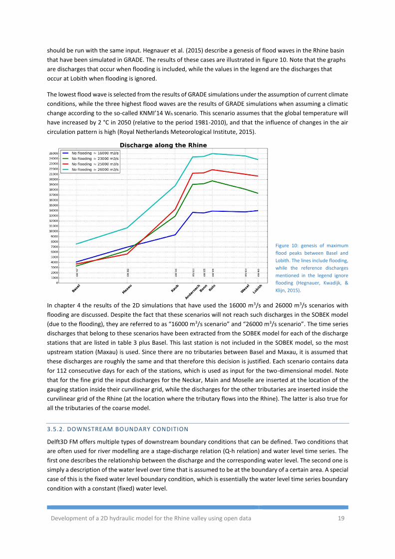
should be run with the same input. Hegnauer et al. (2015) describe a genesis of flood waves in the Rhine basin
that have been simulated in GRADE. The results of these cases are illustrated in figure 10. Note that the graphs
are discharges that occur when flooding is included, while the values in the legend are the discharges that
occur at Lobith when flooding is ignored.
The lowest flood wave is selected from the results of GRADE simulations under the assumption of current climate
conditions, while the three highest flood waves are the results of GRADE simulations when assuming a climatic
change according to the so-called KNMI’14 Wh scenario. This scenario assumes that the global temperature will
have increased by 2 °C in 2050 (relative to the period 1981-2010), and that the influence of changes in the air
circulation pattern is high (Royal Netherlands Meteorological Institute, 2015).
Figure 10: genesis of maximum
flood peaks between Basel and
Lobith. The lines include flooding,
while the reference discharges
mentioned in the legend ignore
flooding (Hegnauer, Kwadijk, &
Klijn, 2015).
In chapter 4 the results of the 2D simulations that have used the 16000 m3/s and 26000 m3/s scenarios with
flooding are discussed. Despite the fact that these scenarios will not reach such discharges in the SOBEK model
(due to the flooding), they are referred to as “16000 m3/s scenario” and “26000 m3/s scenario”. The time series
discharges that belong to these scenarios have been extracted from the SOBEK model for each of the discharge
stations that are listed in table 3 plus Basel. This last station is not included in the SOBEK model, so the most
upstream station (Maxau) is used. Since there are no tributaries between Basel and Maxau, it is assumed that
these discharges are roughly the same and that therefore this decision is justified. Each scenario contains data
for 112 consecutive days for each of the stations, which is used as input for the two-dimensional model. Note
that for the fine grid the input discharges for the Neckar, Main and Moselle are inserted at the location of the
gauging station inside their curvilinear grid, while the discharges for the other tributaries are inserted inside the
curvilinear grid of the Rhine (at the location where the tributary flows into the Rhine). The latter is also true for
all the tributaries of the coarse model.
3.5.2. DOWNSTREAM BOUNDARY CONDITION
Delft3D FM offers multiple types of downstream boundary conditions that can be defined. Two conditions that
are often used for river modelling are a stage-discharge relation (Q-h relation) and water level time series. The
first one describes the relationship between the discharge and the corresponding water level. The second one is
simply a description of the water level over time that is assumed to be at the boundary of a certain area. A special
case of this is the fixed water level boundary condition, which is essentially the water level time series boundary
condition with a constant (fixed) water level.
BSc Thesis – Martijn Kriebel 20
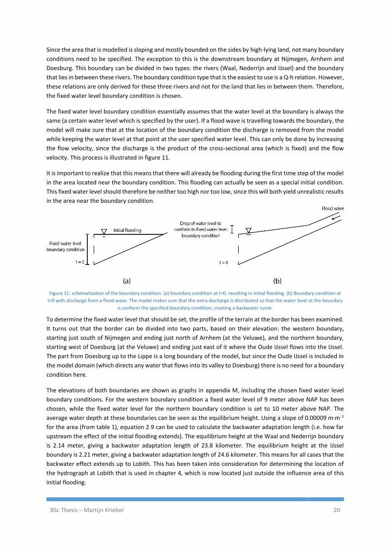
Since the area that is modelled is sloping and mostly bounded on the sides by high-lying land, not many boundary
conditions need to be specified. The exception to this is the downstream boundary at Nijmegen, Arnhem and
Doesburg. This boundary can be divided in two types: the rivers (Waal, Nederrijn and IJssel) and the boundary
that lies in between these rivers. The boundary condition type that is the easiest to use is a Q-h relation. However,
these relations are only derived for these three rivers and not for the land that lies in between them. Therefore,
the fixed water level boundary condition is chosen.
The fixed water level boundary condition essentially assumes that the water level at the boundary is always the
same (a certain water level which is specified by the user). If a flood wave is travelling towards the boundary, the
model will make sure that at the location of the boundary condition the discharge is removed from the model
while keeping the water level at that point at the user specified water level. This can only be done by increasing
the flow velocity, since the discharge is the product of the cross-sectional area (which is fixed) and the flow
velocity. This process is illustrated in figure 11.
It is important to realize that this means that there will already be flooding during the first time step of the model
in the area located near the boundary condition. This flooding can actually be seen as a special initial condition.
This fixed water level should therefore be neither too high nor too low, since this will both yield unrealistic results
in the area near the boundary condition.
Figure 11: schematization of the boundary condition. (a) boundary condition at t=0, resulting in initial flooding. (b) Boundary condition at
t>0 with discharge from a flood wave. The model makes sure that the extra discharge is distributed so that the water level at the boundary
is conform the specified boundary condition, creating a backwater curve.
To determine the fixed water level that should be set, the profile of the terrain at the border has been examined.
It turns out that the border can be divided into two parts, based on their elevation: the western boundary,
starting just south of Nijmegen and ending just north of Arnhem (at the Veluwe), and the northern boundary,
starting west of Doesburg (at the Veluwe) and ending just east of it where the Oude IJssel flows into the IJssel.
The part from Doesburg up to the Lippe is a long boundary of the model, but since the Oude IJssel is included in
the model domain (which directs any water that flows into its valley to Doesburg) there is no need for a boundary
condition here.
The elevations of both boundaries are shown as graphs in appendix M, including the chosen fixed water level
boundary conditions. For the western boundary condition a fixed water level of 9 meter above NAP has been
chosen, while the fixed water level for the northern boundary condition is set to 10 meter above NAP. The
average water depth at these boundaries can be seen as the equilibrium height. Using a slope of 0.00009 m·m-1
for the area (from table 1), equation 2.9 can be used to calculate the backwater adaptation length (i.e. how far
upstream the effect of the initial flooding extends). The equilibrium height at the Waal and Nederrijn boundary
is 2.14 meter, giving a backwater adaptation length of 23.8 kilometer. The equilibrium height at the IJssel
boundary is 2.21 meter, giving a backwater adaptation length of 24.6 kilometer. This means for all cases that the
backwater effect extends up to Lobith. This has been taken into consideration for determining the location of
the hydrograph at Lobith that is used in chapter 4, which is now located just outside the influence area of this
initial flooding.
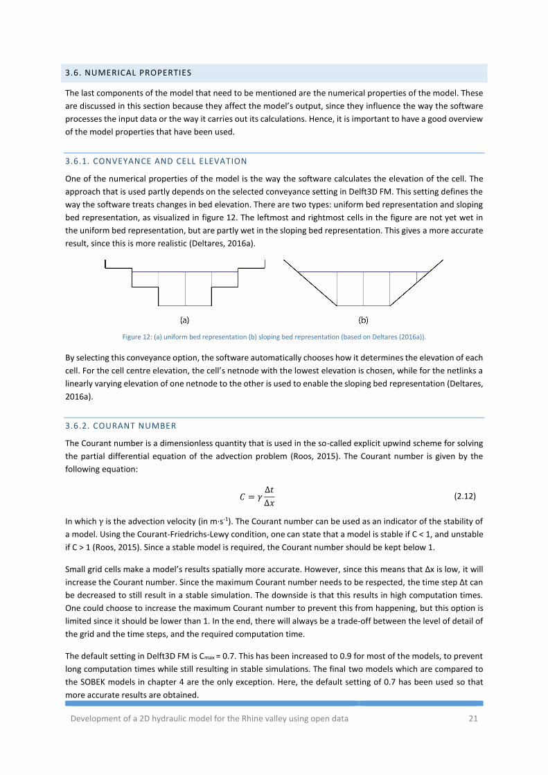
Development of a 2D hydraulic model for the Rhine valley using open data 21
3.6. NUMERICAL PROPERTIES
The last components of the model that need to be mentioned are the numerical properties of the model. These
are discussed in this section because they affect the model’s output, since they influence the way the software
processes the input data or the way it carries out its calculations. Hence, it is important to have a good overview
of the model properties that have been used.
3.6.1. CONVEYANCE AND CELL ELEVATION
One of the numerical properties of the model is the way the software calculates the elevation of the cell. The
approach that is used partly depends on the selected conveyance setting in Delft3D FM. This setting defines the
way the software treats changes in bed elevation. There are two types: uniform bed representation and sloping
bed representation, as visualized in figure 12. The leftmost and rightmost cells in the figure are not yet wet in
the uniform bed representation, but are partly wet in the sloping bed representation. This gives a more accurate
result, since this is more realistic (Deltares, 2016a).
Figure 12: (a) uniform bed representation (b) sloping bed representation (based on Deltares (2016a)).
By selecting this conveyance option, the software automatically chooses how it determines the elevation of each
cell. For the cell centre elevation, the cell’s netnode with the lowest elevation is chosen, while for the netlinks a
linearly varying elevation of one netnode to the other is used to enable the sloping bed representation (Deltares,
2016a).
3.6.2. COURANT NUMBER
The Courant number is a dimensionless quantity that is used in the so-called explicit upwind scheme for solving
the partial differential equation of the advection problem (Roos, 2015). The Courant number is given by the
following equation:
𝐶 = 𝛾∆𝑡
∆𝑥 (2.12)
In which γ is the advection velocity (in m·s-1). The Courant number can be used as an indicator of the stability of
a model. Using the Courant-Friedrichs-Lewy condition, one can state that a model is stable if C < 1, and unstable
if C > 1 (Roos, 2015). Since a stable model is required, the Courant number should be kept below 1.
Small grid cells make a model’s results spatially more accurate. However, since this means that Δx is low, it will
increase the Courant number. Since the maximum Courant number needs to be respected, the time step Δt can
be decreased to still result in a stable simulation. The downside is that this results in high computation times.
One could choose to increase the maximum Courant number to prevent this from happening, but this option is
limited since it should be lower than 1. In the end, there will always be a trade-off between the level of detail of
the grid and the time steps, and the required computation time.
The default setting in Delft3D FM is Cmax = 0.7. This has been increased to 0.9 for most of the models, to prevent
long computation times while still resulting in stable simulations. The final two models which are compared to
the SOBEK models in chapter 4 are the only exception. Here, the default setting of 0.7 has been used so that
more accurate results are obtained.

BSc Thesis – Martijn Kriebel 22
4. RESULTS
The table below gives an overview of the different models that have been run. The two-dimensional models are
compared for three different properties, which can give more information of the effects of these properties on
the model output. Furthermore, two “final” 2D models are used for comparison with the 1D SOBEK model from
GRADE. As mentioned in chapter 3.5.1, note that the 16000 m3/s and 26000 m3/s are the SOBEK scenarios with
flooding, meaning that the discharges from the SOBEK model will be lower than those numbers. A summary of
the different models can be found in the table below. All simulations have been run using a 4 core Intel Xeon E5-
2670 processor and 16 GB RAM.
Comparison properties 2D model
Coarse grid
vs.
Fine grid Goal:
Computational cells: 83878 (see table 4 for more details)
Initial water depth: 3 meter Initial discharges: yes Input scenario: 26000 m3/s Courant number: 0.9 Run time: 4h12m
Computational cells: 124825 (see table 4 for more details)
Initial water depth: 3 meter Initial discharges: yes Input scenario: 26000 m3/s Courant number: 0.9 Run time: 16h19m
To find out what effect the type of grid has on the
model output.
2.5 meter initial water depth
vs.
3 meter initial water depth Goal:
Grid: coarse Initial water depth: 2.5 meter Initial discharges: yes Input scenario: 26000 m3/s Courant number: 0.9 Run time: 4h11m
Grid: coarse Initial water depth: 3 meter Initial discharges: yes Input scenario: 26000 m3/s Courant number: 0.9 Run time: 4h12m Note that this model is the same as the coarse grid model in the top left corner.
To find out what effect the initial water depth has on
the model output.
Initial discharges
vs.
No initial discharges Goal:
Grid: coarse Initial water depth: 3 meter Initial discharges: yes Input scenario: 26000 m3/s Courant number: 0.9 Run time: 4h12m Note that this model is the same as the coarse grid model in the top left corner.
Grid: coarse Initial water depth: 3 meter Initial discharges: no Input scenario: 26000 m3/s Courant number: 0.9 Run time: 4h09m
To find out what the effects of initial discharges (and consequently initial velocities) from a restart
file are on the model output.
Comparison 2D Delft3D FM model vs. 1D SOBEK model
2D D3D FM 16000 m3/s scenario
vs.
1D SOBEK 16000 m3/s scenario Goal:
Grid: coarse Initial water depth: 3 meter Initial discharges: yes Input scenario: 16000 m3/s Courant number: 0.7 Run time: 4h52m
Input scenario: 16000 m3/s (with flooding) Run time: 2m
To find out how the 2D simulations in Delft3D FM differ from the 1D SOBEK
model of GRADE.
2D D3D FM 26000 m3/s scenario
vs.
1D SOBEK 26000 m3/s scenario
Grid: coarse Initial water depth: 3 meter Initial discharges: yes Input scenario: 26000 m3/s Courant number: 0.7 Run time: 5h10m
Input scenario: 26000 m3/s (with flooding)
Run time: 2m
Table 5: overview of the comparisons between models that have been made.
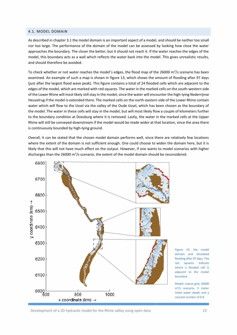
Development of a 2D hydraulic model for the Rhine valley using open data 23
4.1. MODEL DOMAIN
As described in chapter 3.1 the model domain is an important aspect of a model, and should be neither too small
nor too large. The performance of the domain of the model can be assessed by looking how close the water
approaches the boundary. The closer the better, but it should not reach it. If the water reaches the edges of the
model, this boundary acts as a wall which reflects the water back into the model. This gives unrealistic results,
and should therefore be avoided.
To check whether or not water reaches the model’s edges, the flood map of the 26000 m3/s scenario has been
examined. An example of such a map is shown in figure 13, which shows the amount of flooding after 97 days
(just after the largest flood wave peak). This figure contains a total of 24 flooded cells which are adjacent to the
edges of the model, which are marked with red squares. The water in the marked cells on the south-western side
of the Lower Rhine will most likely still stay in the model, since the water will encounter the high-lying Nederrijnse
Heuvelrug if the model is extended there. The marked cells on the north-eastern side of the Lower Rhine contain
water which will flow to the IJssel via the valley of the Oude IJssel, which has been chosen as the boundary of
the model. The water in these cells will stay in the model, but will most likely flow a couple of kilometers further
to the boundary condition at Doesburg where it is removed. Lastly, the water in the marked cells at the Upper
Rhine will still be conveyed downstream if the model would be made wider at that location, since the area there
is continuously bounded by high-lying ground.
Overall, it can be stated that the chosen model domain performs well, since there are relatively few locations
where the extent of the domain is not sufficient enough. One could choose to widen the domain here, but it is
likely that this will not have much effect on the output. However, if one wants to model scenarios with higher
discharges than the 26000 m3/s scenario, the extent of the model domain should be reconsidered.
Figure 13: the model
domain and simulated
flooding after 97 days. The
red squares indicate
where a flooded cell is
adjacent to the model
boundary.
Model: coarse grid, 26000
m3/s scenario, 3 meter
initial water depth and a
courant number of 0.9.
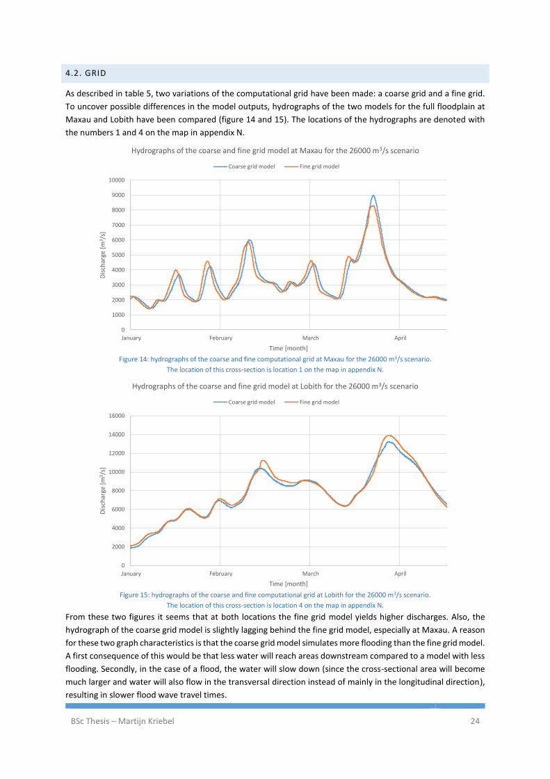
BSc Thesis – Martijn Kriebel 24
4.2. GRID
As described in table 5, two variations of the computational grid have been made: a coarse grid and a fine grid.
To uncover possible differences in the model outputs, hydrographs of the two models for the full floodplain at
Maxau and Lobith have been compared (figure 14 and 15). The locations of the hydrographs are denoted with
the numbers 1 and 4 on the map in appendix N.
Figure 14: hydrographs of the coarse and fine computational grid at Maxau for the 26000 m3/s scenario.
The location of this cross-section is location 1 on the map in appendix N.
Figure 15: hydrographs of the coarse and fine computational grid at Lobith for the 26000 m3/s scenario.
The location of this cross-section is location 4 on the map in appendix N.
From these two figures it seems that at both locations the fine grid model yields higher discharges. Also, the
hydrograph of the coarse grid model is slightly lagging behind the fine grid model, especially at Maxau. A reason
for these two graph characteristics is that the coarse grid model simulates more flooding than the fine grid model.
A first consequence of this would be that less water will reach areas downstream compared to a model with less
flooding. Secondly, in the case of a flood, the water will slow down (since the cross-sectional area will become
much larger and water will also flow in the transversal direction instead of mainly in the longitudinal direction),
resulting in slower flood wave travel times.
0
1000
2000
3000
4000
5000
6000
7000
8000
9000
10000
January February March April
Dis
char
ge [
m3/s
]
Time [month]
Hydrographs of the coarse and fine grid model at Maxau for the 26000 m3/s scenario
Coarse grid model Fine grid model
0
2000
4000
6000
8000
10000
12000
14000
16000
January February March April
Dis
char
ge [
m3/s
]
Time [month]
Hydrographs of the coarse and fine grid model at Lobith for the 26000 m3/s scenario
Coarse grid model Fine grid model
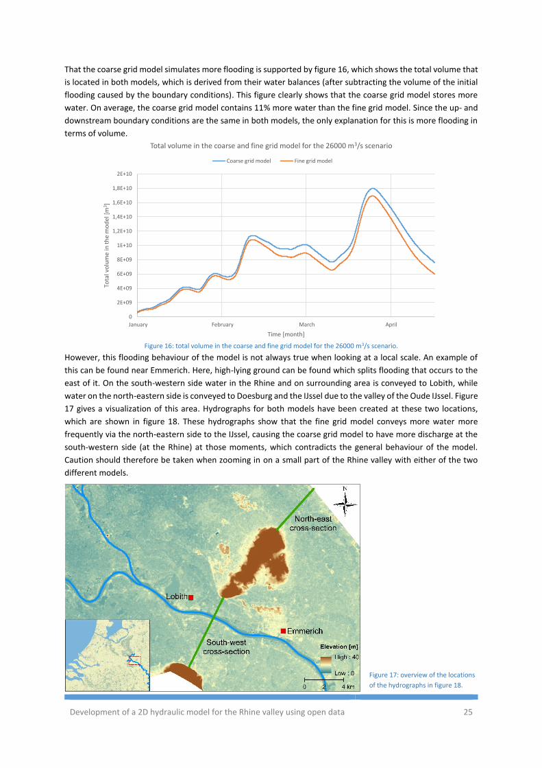
Development of a 2D hydraulic model for the Rhine valley using open data 25
That the coarse grid model simulates more flooding is supported by figure 16, which shows the total volume that
is located in both models, which is derived from their water balances (after subtracting the volume of the initial
flooding caused by the boundary conditions). This figure clearly shows that the coarse grid model stores more
water. On average, the coarse grid model contains 11% more water than the fine grid model. Since the up- and
downstream boundary conditions are the same in both models, the only explanation for this is more flooding in
terms of volume.
Figure 16: total volume in the coarse and fine grid model for the 26000 m3/s scenario.
However, this flooding behaviour of the model is not always true when looking at a local scale. An example of
this can be found near Emmerich. Here, high-lying ground can be found which splits flooding that occurs to the
east of it. On the south-western side water in the Rhine and on surrounding area is conveyed to Lobith, while
water on the north-eastern side is conveyed to Doesburg and the IJssel due to the valley of the Oude IJssel. Figure
17 gives a visualization of this area. Hydrographs for both models have been created at these two locations,
which are shown in figure 18. These hydrographs show that the fine grid model conveys more water more
frequently via the north-eastern side to the IJssel, causing the coarse grid model to have more discharge at the
south-western side (at the Rhine) at those moments, which contradicts the general behaviour of the model.
Caution should therefore be taken when zooming in on a small part of the Rhine valley with either of the two
different models.
Figure 17: overview of the locations
of the hydrographs in figure 18.
0
2E+09
4E+09
6E+09
8E+09
1E+10
1,2E+10
1,4E+10
1,6E+10
1,8E+10
2E+10
January February March April
Tota
l vo
lum
e in
th
e m
od
el [
m3]
Time [month]
Total volume in the coarse and fine grid model for the 26000 m3/s scenario
Coarse grid model Fine grid model
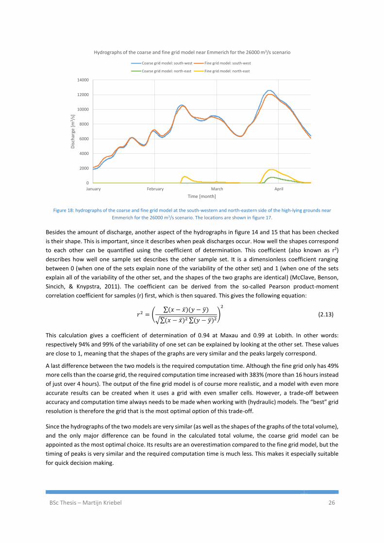
BSc Thesis – Martijn Kriebel 26
Figure 18: hydrographs of the coarse and fine grid model at the south-western and north-eastern side of the high-lying grounds near
Emmerich for the 26000 m3/s scenario. The locations are shown in figure 17.
Besides the amount of discharge, another aspect of the hydrographs in figure 14 and 15 that has been checked
is their shape. This is important, since it describes when peak discharges occur. How well the shapes correspond
to each other can be quantified using the coefficient of determination. This coefficient (also known as r2)
describes how well one sample set describes the other sample set. It is a dimensionless coefficient ranging
between 0 (when one of the sets explain none of the variability of the other set) and 1 (when one of the sets
explain all of the variability of the other set, and the shapes of the two graphs are identical) (McClave, Benson,
Sincich, & Knypstra, 2011). The coefficient can be derived from the so-called Pearson product-moment
correlation coefficient for samples (r) first, which is then squared. This gives the following equation:
𝑟2 = (∑(𝑥 − �̅�)(𝑦 − �̅�)
√∑(𝑥 − �̅�)2 ∑(𝑦 − �̅�)2)
2
(2.13)
This calculation gives a coefficient of determination of 0.94 at Maxau and 0.99 at Lobith. In other words:
respectively 94% and 99% of the variability of one set can be explained by looking at the other set. These values
are close to 1, meaning that the shapes of the graphs are very similar and the peaks largely correspond.
A last difference between the two models is the required computation time. Although the fine grid only has 49%
more cells than the coarse grid, the required computation time increased with 383% (more than 16 hours instead
of just over 4 hours). The output of the fine grid model is of course more realistic, and a model with even more
accurate results can be created when it uses a grid with even smaller cells. However, a trade-off between
accuracy and computation time always needs to be made when working with (hydraulic) models. The “best” grid
resolution is therefore the grid that is the most optimal option of this trade-off.
Since the hydrographs of the two models are very similar (as well as the shapes of the graphs of the total volume),
and the only major difference can be found in the calculated total volume, the coarse grid model can be
appointed as the most optimal choice. Its results are an overestimation compared to the fine grid model, but the
timing of peaks is very similar and the required computation time is much less. This makes it especially suitable
for quick decision making.
0
2000
4000
6000
8000
10000
12000
14000
January February March April
Dis
char
ge [
m3 /
s]
Time [month]
Hydrographs of the coarse and fine grid model near Emmerich for the 26000 m3/s scenario
Coarse grid model: south-west Fine grid model: south-west
Coarse grid model: north-east Fine grid model: north-east
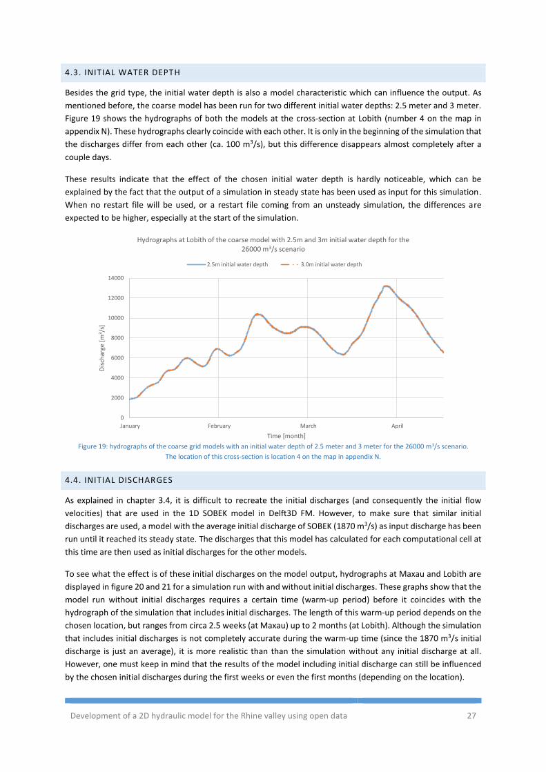
Development of a 2D hydraulic model for the Rhine valley using open data 27
4.3. INITIAL WATER DEPTH
Besides the grid type, the initial water depth is also a model characteristic which can influence the output. As
mentioned before, the coarse model has been run for two different initial water depths: 2.5 meter and 3 meter.
Figure 19 shows the hydrographs of both the models at the cross-section at Lobith (number 4 on the map in
appendix N). These hydrographs clearly coincide with each other. It is only in the beginning of the simulation that
the discharges differ from each other (ca. 100 m3/s), but this difference disappears almost completely after a
couple days.
These results indicate that the effect of the chosen initial water depth is hardly noticeable, which can be
explained by the fact that the output of a simulation in steady state has been used as input for this simulation.
When no restart file will be used, or a restart file coming from an unsteady simulation, the differences are
expected to be higher, especially at the start of the simulation.
Figure 19: hydrographs of the coarse grid models with an initial water depth of 2.5 meter and 3 meter for the 26000 m3/s scenario.
The location of this cross-section is location 4 on the map in appendix N.
4.4. INITIAL DISCHARGES
As explained in chapter 3.4, it is difficult to recreate the initial discharges (and consequently the initial flow
velocities) that are used in the 1D SOBEK model in Delft3D FM. However, to make sure that similar initial
discharges are used, a model with the average initial discharge of SOBEK (1870 m3/s) as input discharge has been
run until it reached its steady state. The discharges that this model has calculated for each computational cell at
this time are then used as initial discharges for the other models.
To see what the effect is of these initial discharges on the model output, hydrographs at Maxau and Lobith are
displayed in figure 20 and 21 for a simulation run with and without initial discharges. These graphs show that the
model run without initial discharges requires a certain time (warm-up period) before it coincides with the
hydrograph of the simulation that includes initial discharges. The length of this warm-up period depends on the
chosen location, but ranges from circa 2.5 weeks (at Maxau) up to 2 months (at Lobith). Although the simulation
that includes initial discharges is not completely accurate during the warm-up time (since the 1870 m3/s initial
discharge is just an average), it is more realistic than than the simulation without any initial discharge at all.
However, one must keep in mind that the results of the model including initial discharge can still be influenced
by the chosen initial discharges during the first weeks or even the first months (depending on the location).
0
2000
4000
6000
8000
10000
12000
14000
January February March April
Dis
char
ge [
m3/s
]
Time [month]
Hydrographs at Lobith of the coarse model with 2.5m and 3m initial water depth for the 26000 m3/s scenario
2.5m initial water depth 3.0m initial water depth
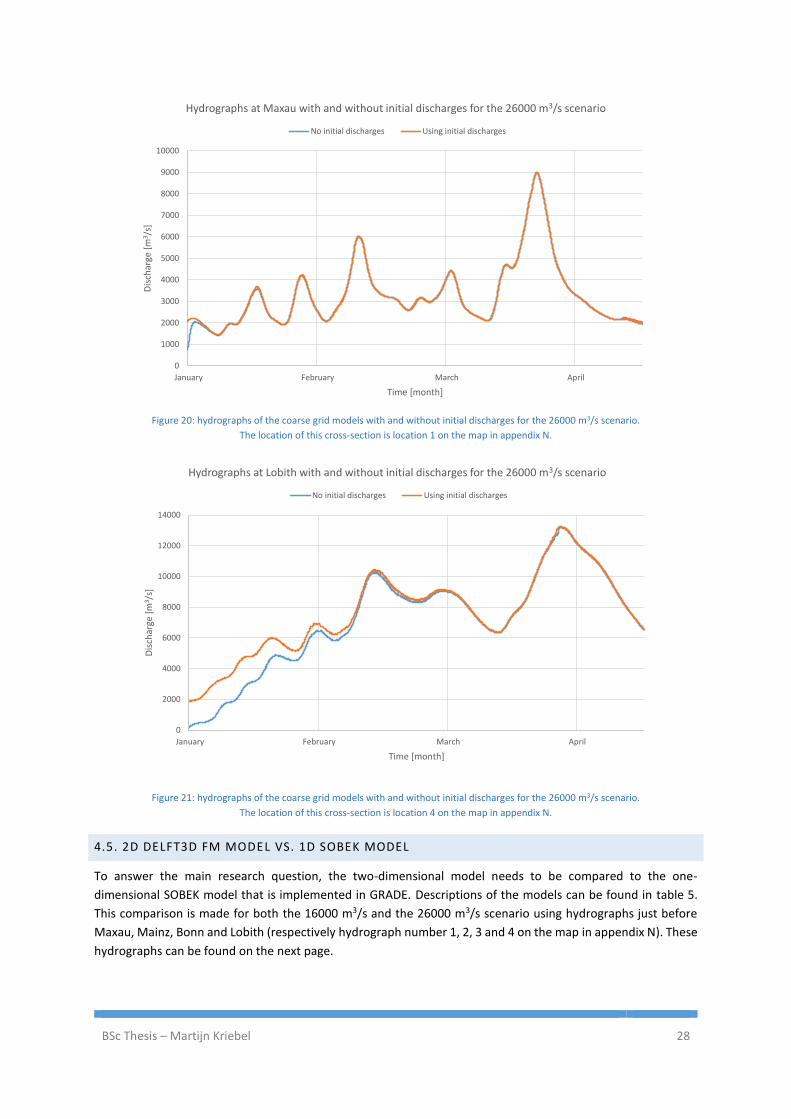
BSc Thesis – Martijn Kriebel 28
Figure 20: hydrographs of the coarse grid models with and without initial discharges for the 26000 m3/s scenario.
The location of this cross-section is location 1 on the map in appendix N.
Figure 21: hydrographs of the coarse grid models with and without initial discharges for the 26000 m3/s scenario.
The location of this cross-section is location 4 on the map in appendix N.
4.5. 2D DELFT3D FM MODEL VS. 1D SOBEK MODEL
To answer the main research question, the two-dimensional model needs to be compared to the one-
dimensional SOBEK model that is implemented in GRADE. Descriptions of the models can be found in table 5.
This comparison is made for both the 16000 m3/s and the 26000 m3/s scenario using hydrographs just before
Maxau, Mainz, Bonn and Lobith (respectively hydrograph number 1, 2, 3 and 4 on the map in appendix N). These
hydrographs can be found on the next page.
0
1000
2000
3000
4000
5000
6000
7000
8000
9000
10000
January February March April
Dis
char
ge [
m3/s
]
Time [month]
Hydrographs at Maxau with and without initial discharges for the 26000 m3/s scenario
No initial discharges Using initial discharges
0
2000
4000
6000
8000
10000
12000
14000
January February March April
Dis
char
ge [
m3/s
]
Time [month]
Hydrographs at Lobith with and without initial discharges for the 26000 m3/s scenario
No initial discharges Using initial discharges
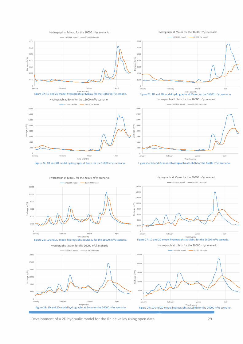
Development of a 2D hydraulic model for the Rhine valley using open data 29
Figure 22: 1D and 2D model hydrographs at Maxau for the 16000 m3/s scenario.
0
1000
2000
3000
4000
5000
6000
7000
January February March April
Dis
char
ge [
m3/s
]
Time [month]
Hydrograph at Maxau for the 16000 m3/s scenario
1D SOBEK model 2D D3D FM model
Figure 23: 1D and 2D model hydrographs at Mainz for the 16000 m3/s scenario.
0
1000
2000
3000
4000
5000
6000
7000
January February March April
Dis
char
ge [
m3/s
]
Time [month]
Hydrograph at Mainz for the 16000 m3/s scenario
1D SOBEK model 2D D3D FM model
Figure 24: 1D and 2D model hydrographs at Bonn for the 16000 m3/s scenario.
0
2000
4000
6000
8000
10000
12000
14000
16000
January February March April
Dis
char
ge [
m3/s
]
Time [month]
Hydrograph at Bonn for the 16000 m3/s scenario
1D SOBEK model 2D D3D FM model
Figure 25: 1D and 2D model hydrographs at Lobith for the 16000 m3/s scenario.
0
2000
4000
6000
8000
10000
12000
14000
16000
January February March April
Dis
char
ge [
m3/s
]
Time [month]
Hydrograph at Lobith for the 16000 m3/s scenario
1D SOBEK model 2D D3D FM model
Figure 26: 1D and 2D model hydrographs at Maxau for the 26000 m3/s scenario.
0
2000
4000
6000
8000
10000
12000
January February March April
Dis
char
ge [
m3/s
]
Time [month]
Hydrograph at Maxau for the 26000 m3/s scenario
1D SOBEK model 2D D3D FM model
Figure 27: 1D and 2D model hydrographs at Mainz for the 26000 m3/s scenario.
0
2000
4000
6000
8000
10000
12000
14000
16000
January February March April
Dis
char
ge [
m3/s
]
Time [month]
Hydrograph at Mainz for the 26000 m3/s scenario
1D SOBEK model 2D D3D FM model
Figure 29: 1D and 2D model hydrographs at Lobith for the 26000 m3/s scenario.
0
5000
10000
15000
20000
25000
January February March April
Dis
char
ge [
m3/s
]
Time [month]
Hydrograph at Lobith for the 26000 m3/s scenario
1D SOBEK model 2D D3D FM model
Figure 28: 1D and 2D model hydrographs at Bonn for the 26000 m3/s scenario.
0
5000
10000
15000
20000
25000
30000
January February March April
Dis
char
ge [
m3/s
]
Time [month]
Hydrograph at Bonn for the 26000 m3/s scenario
1D SOBEK model 2D D3D FM model
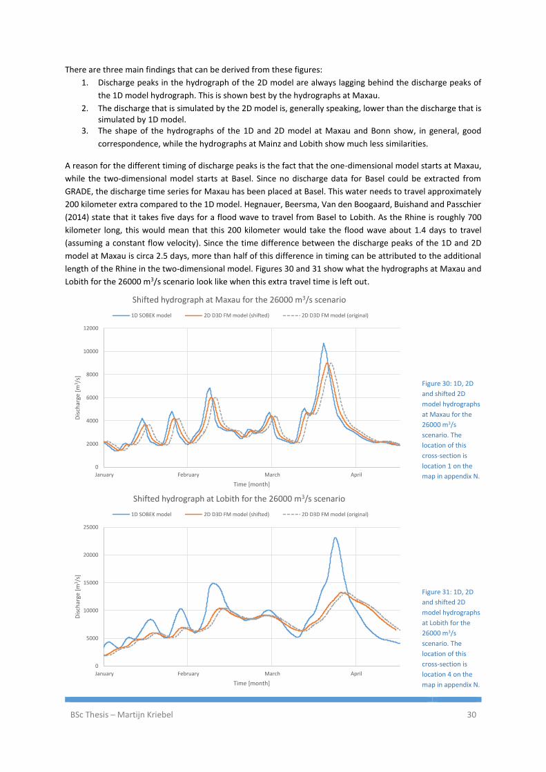
BSc Thesis – Martijn Kriebel 30
There are three main findings that can be derived from these figures:
1. Discharge peaks in the hydrograph of the 2D model are always lagging behind the discharge peaks of
the 1D model hydrograph. This is shown best by the hydrographs at Maxau.
2. The discharge that is simulated by the 2D model is, generally speaking, lower than the discharge that is simulated by 1D model.
3. The shape of the hydrographs of the 1D and 2D model at Maxau and Bonn show, in general, good
correspondence, while the hydrographs at Mainz and Lobith show much less similarities.
A reason for the different timing of discharge peaks is the fact that the one-dimensional model starts at Maxau,
while the two-dimensional model starts at Basel. Since no discharge data for Basel could be extracted from
GRADE, the discharge time series for Maxau has been placed at Basel. This water needs to travel approximately
200 kilometer extra compared to the 1D model. Hegnauer, Beersma, Van den Boogaard, Buishand and Passchier
(2014) state that it takes five days for a flood wave to travel from Basel to Lobith. As the Rhine is roughly 700
kilometer long, this would mean that this 200 kilometer would take the flood wave about 1.4 days to travel
(assuming a constant flow velocity). Since the time difference between the discharge peaks of the 1D and 2D
model at Maxau is circa 2.5 days, more than half of this difference in timing can be attributed to the additional
length of the Rhine in the two-dimensional model. Figures 30 and 31 show what the hydrographs at Maxau and
Lobith for the 26000 m3/s scenario look like when this extra travel time is left out.
Figure 30: 1D, 2D
and shifted 2D
model hydrographs
at Maxau for the
26000 m3/s
scenario. The
location of this
cross-section is
location 1 on the
map in appendix N.
Figure 31: 1D, 2D
and shifted 2D
model hydrographs
at Lobith for the
26000 m3/s
scenario. The
location of this
cross-section is
location 4 on the
map in appendix N.
0
2000
4000
6000
8000
10000
12000
January February March April
Dis
char
ge [
m3/s
]
Time [month]
Shifted hydrograph at Maxau for the 26000 m3/s scenario
1D SOBEK model 2D D3D FM model (shifted) 2D D3D FM model (original)
0
5000
10000
15000
20000
25000
January February March April
Dis
char
ge [
m3/s
]
Time [month]
Shifted hydrograph at Lobith for the 26000 m3/s scenario
1D SOBEK model 2D D3D FM model (shifted) 2D D3D FM model (original)
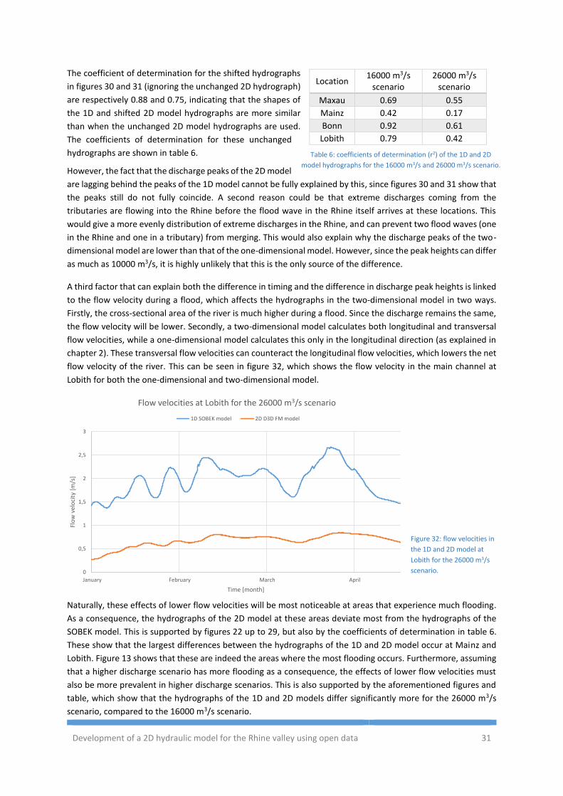
Development of a 2D hydraulic model for the Rhine valley using open data 31
The coefficient of determination for the shifted hydrographs
in figures 30 and 31 (ignoring the unchanged 2D hydrograph)
are respectively 0.88 and 0.75, indicating that the shapes of
the 1D and shifted 2D model hydrographs are more similar
than when the unchanged 2D model hydrographs are used.
The coefficients of determination for these unchanged
hydrographs are shown in table 6.
However, the fact that the discharge peaks of the 2D model
are lagging behind the peaks of the 1D model cannot be fully explained by this, since figures 30 and 31 show that
the peaks still do not fully coincide. A second reason could be that extreme discharges coming from the
tributaries are flowing into the Rhine before the flood wave in the Rhine itself arrives at these locations. This
would give a more evenly distribution of extreme discharges in the Rhine, and can prevent two flood waves (one
in the Rhine and one in a tributary) from merging. This would also explain why the discharge peaks of the two-
dimensional model are lower than that of the one-dimensional model. However, since the peak heights can differ
as much as 10000 m3/s, it is highly unlikely that this is the only source of the difference.
A third factor that can explain both the difference in timing and the difference in discharge peak heights is linked
to the flow velocity during a flood, which affects the hydrographs in the two-dimensional model in two ways.
Firstly, the cross-sectional area of the river is much higher during a flood. Since the discharge remains the same,
the flow velocity will be lower. Secondly, a two-dimensional model calculates both longitudinal and transversal
flow velocities, while a one-dimensional model calculates this only in the longitudinal direction (as explained in
chapter 2). These transversal flow velocities can counteract the longitudinal flow velocities, which lowers the net
flow velocity of the river. This can be seen in figure 32, which shows the flow velocity in the main channel at
Lobith for both the one-dimensional and two-dimensional model.
Figure 32: flow velocities in
the 1D and 2D model at
Lobith for the 26000 m3/s
scenario.
Naturally, these effects of lower flow velocities will be most noticeable at areas that experience much flooding.
As a consequence, the hydrographs of the 2D model at these areas deviate most from the hydrographs of the
SOBEK model. This is supported by figures 22 up to 29, but also by the coefficients of determination in table 6.
These show that the largest differences between the hydrographs of the 1D and 2D model occur at Mainz and
Lobith. Figure 13 shows that these are indeed the areas where the most flooding occurs. Furthermore, assuming
that a higher discharge scenario has more flooding as a consequence, the effects of lower flow velocities must
also be more prevalent in higher discharge scenarios. This is also supported by the aforementioned figures and
table, which show that the hydrographs of the 1D and 2D models differ significantly more for the 26000 m3/s
scenario, compared to the 16000 m3/s scenario.
Location 16000 m3/s
scenario 26000 m3/s
scenario
Maxau 0.69 0.55
Mainz 0.42 0.17
Bonn 0.92 0.61
Lobith 0.79 0.42
Table 6: coefficients of determination (r2) of the 1D and 2D
model hydrographs for the 16000 m3/s and 26000 m3/s scenario.
0
0,5
1
1,5
2
2,5
3
January February March April
Flo
w v
elo
city
[m
/s]
Time [month]
Flow velocities at Lobith for the 26000 m3/s scenario
1D SOBEK model 2D D3D FM model
BSc Thesis – Martijn Kriebel 32
5. DISCUSSION
This chapter reflects on the methodology that is used during this study. Although a two-dimensional hydraulic
model has been successfully created and compared to the one-dimensional SOBEK model, the methods that have
been used to achieve this and its results need to be evaluated carefully. This chapter therefore discusses the
most important uncertainties in this study that could influence the results, while chapter 7 gives
recommendations based on this discussion for future studies.
The majority of this study has been focused on the development of a two-dimensional hydraulic model for the
Rhine valley. This model contains many different components, but the digital elevation model might be the most
significant component of them all. The SRTM DEM is not only used for determining the model extent, but also
plays an important role in the calculations that Delft3D FM carries out. Although comparison with a different
digital elevation model was not possible, it is not unthinkable that errors in this DEM cause (locally) incorrect
results in the simulations, since the SRTM DEM has an absolute height error of 6.2 meter at 90% probability (as
mentioned in chapter 3.2).
Besides this absolute error in the SRTM DEM, it must not be forgotten that the DEM has been manually modified
in order to make it suitable for hydraulic modelling. The most notable modification is the incorporation of
bathymetry of the Rhine that was needed, since this is not included in the DEM. As explained in chapter 3.2.2 a
rectangular channel with a constant channel depth of 3 meter is assumed, based on the average water depth
that is measured over a period of ten years. However, this is most likely either an over- or underestimation for
most parts of the Rhine, and not a completely realistic representation. Furthermore, the Rhine will, in reality,
never be a perfectly rectangular channel.
A third DEM-related point of discussion is the omission of tributary bathymetry. Because this is not included, the
model simulates the elevation of any water at these locations higher than it would be in reality, since the DEM
values here are the elevation values of the tributary water surface. This is not realistic, and the effect of this
might influence the simulation results at the locations of these tributaries. However, it is questionable whether
or not this has any significant effect on the simulation results of the Rhine as a whole.
Another point of discussion concerns the chosen friction coefficient. To incorporate roughness in the model, a
friction coefficient need to be specified which differs for each type of land use. For the simulation runs during
this study, the default Manning friction coefficient in Delft3D FM has been used, which is 0.023. However, it is
most likely that this is an underestimation for most of the study area, since areas that contain forests, cultivated
land etc. have a much higher coefficient.
Uncertainty in the comparison of the one- and two-dimensional models can be found in the chosen initial
conditions. As discussed in chapter 4.3 the chosen initial water depth will not have much influence on the results
of the two-dimensional model. However, there is a certain measureable difference. Furthermore, the results of
the restart file which are used as input for the two-dimensional model rely heavily on the chosen initial discharge.
The initial discharge that has been used is chosen under the assumption that it is the best approximation of the
initial discharges that are used in the one-dimensional model.
Lastly, there are some aspects of the two-dimensional model that have not been considered in this study. One
of these are elevated line elements in the study area. Such line elements are often narrow, meaning that they
have not been detected by the SRTM, and therefore not incorporated in the DEM. However, line elements like
dykes are of great importance in a hydraulic model and can influence the results significantly. Furthermore,
Delft3D FM offers multiple features regarding wind, temperature et cetera. Although these can affect the
model’s results, they have not been included.
Development of a 2D hydraulic model for the Rhine valley using open data 33
6. CONCLUSIONS
The main objective of this study was to find out how a two-dimensional hydraulic model that is created in Delft3D
FM compares to a one-dimensional hydraulic model that is created in SOBEK-RE. The components of the
developed two-dimensional hydraulic model that is used for this comparison have been described in chapter 3.
Chapter 4 then discussed the effect of changes in these components on the model output, after which the
differences between a final two-dimensional hydraulic model and the one-dimensional model are discussed. The
main findings from this chapter are summarized below.
Firstly, it can be concluded that the minimum required model extent for an extreme discharge event in the Rhine
valley can be accurately determined by calculating the probable extent of flooding of the river’s floodplains in
combination with calculations on the probable backwater adaptation length that needs to be taken into account
at the tributaries.
Secondly, a two-dimensional hydraulic model that uses a relative fine computational grid (in this study a grid that
contains 49% more computational cells than the so-called coarse grid) simulates on average over one tenth less
volume in the model (i.e. less flooding) compared to a two-dimensional model that uses a coarse grid. As a
consequence of this, the discharges that are simulated by the fine grid model are somewhat higher. However,
compared to the fine grid model, the coarse grid model in this study can be appointed as the most optimal
solution since its computational time is almost four times lower.
As it turns out, changes in the initial water depth only influence the simulated discharges at the start of the
simulation, and cause relatively little difference. The use of a so-called restart file as a starting point for the two-
dimensional model appears to have a significant effect on the simulated discharges. Hydrographs of simulations
with and without restart files show a significant difference during the first 2.5 weeks at Maxau, but these
differences can still be seen up to the first two months of the simulation at Lobith.
Comparison of the one-dimensional model with the two-dimensional model resulted in three main findings:
- Discharge peaks that are simulated by the two-dimensional model arrive later compared to the peaks in the one-dimensional model.
- The discharges that are simulated by the two-dimensional model are, generally speaking, lower than those that are simulated by the one-dimensional model.
- In general, the hydrographs of the one- and two-dimensional models at Maxau and Bonn share the most similarities, while their hydrographs at Mainz and Lobith differ the most.
An important reason for these differences is the fact that the one-dimensional model starts at Maxau, while the
two-dimensional model starts at Basel. Because comparison of the two models was needed, the input of the 1D
model is also used in the 2D model. Since this data did not contain a discharge time series for Basel, the time
series for Maxau has been used here. As a consequence, it takes the water an estimated 1.4 days longer to reach
Lobith compared to the 1D model. This is supported by the hydrographs of the 2D model, which show more
similarities with the hydrographs of the 1D model if they are shifted 1.4 days to compensate for this extra travel
time. This delay can also cause discharge peaks in tributaries to flow into the Rhine before the flood wave in the
Rhine arrives at the tributary, causing the peak discharge to be more spread out over time.
Lastly, the differences can be explained by the fact that the 2D model simulates lower flow velocities than the
1D model. The reason for this is twofold. Firstly, the cross-sectional area of the river is much larger during a flood,
causing the flow velocity to decrease. This increase of cross-sectional area is better simulated by the 2D model.
Secondly, transversal movements that are simulated by the 2D model cause the longitudinal velocity to decrease.
These transversal movements are not simulated by the 1D model, explaining the differences in discharge and
discharge peak timing. This is also the reason why the differences between the 1D and 2D model are the largest
at Mainz and Lobith, since these are the areas that experience the most flooding according to the 2D model.
BSc Thesis – Martijn Kriebel 34
7. RECOMMENDATIONS
Although a two-dimensional hydraulic model has been successfully created and compared to the one-
dimensional SOBEK model, the model can be improved to get more accurate results. These improvements can
either concern modifications of model components that are already implemented, or the addition of extra
components. Therefore, this chapter gives several recommendations for future studies on this subject and for
future use of the developed two-dimensional model.
A first recommendation concerns the digital elevation model that is used in the model. As mentioned in chapter
3.2 the SRTM DEM is suitable for hydraulic modelling, but still contains a significant height error. A solution for
this would be to use a more accurate DEM (such as a LiDAR DEM). However, this may be difficult to acquire for
such a large area. Moreover, a closer examination of the used DEM revealed that it often includes the elevation
of forest canopy instead of the terrain elevation. Such factors can significantly affect the results of the model,
and it is therefore recommended that these inaccuracies are removed from the DEM.
Furthermore, elevated line elements such as dykes should be added to the model. These elements are often not
included in the DEM because they are too narrow, but they could (partially) prevent flooding in some areas. This
would result in a more realistic simulation, and could perhaps result in a better match between the hydrographs
of the one- and two-dimensional models.
A recommendation related to the land uses in the study area is the friction coefficient. At mentioned in the
discussion, the default Manning friction coefficient of Delft3D FM has been used for the simulations in this study.
This coefficient depends normally on the type of land use, but this default value is used uniformly over the study
area. Since this value is relatively low, it is good for future use of the model to specify this coefficient for each
type of land use separately.
In the current model, the Rhine is specified as a three-meter-deep rectangular channel, while no tributary
bathymetry is included at all. In order to get more detailed, realistic bathymetry, it is recommended to use the
cross-sections that are included in the one-dimensional SOBEK model. As mentioned before, these cross-sections
are on average circa 550 meter apart from each other, and are present for both the Rhine and its tributaries.
When these cross-sections are interpolated, a much more accurate bathymetry is obtained which can be
implemented in the two-dimensional model.
The last recommendation concerns the initial discharges that are used. As described in chapter 3.4 initial these
discharges have been derived from a different simulation using a restart-file, but rely heavily on the chosen
discharge time series of that simulation. The discharge time series that is used has been chosen is assumed to be
the best approximation of the initial discharges that are used in the one-dimensional model. Despite this, it may
well be that different initial conditions result in a more realistic output. However, this should be further studied.
Development of a 2D hydraulic model for the Rhine valley using open data 35
REFERENCES
Bates, P., & De Roo, A. (2000). A simple raster-based model for flood inundation simulation. Journal of
Hydrology, 236(1), 54-77.
Becker, B. P., Schwanenberg, D., Hatz, M., & Schruff, T. (2012). Conjuctive Real Time Control And Hydrodynamic
Modelling In Application To Rhine River. 10th International Conference on Hydroinformatics. Hamburg:
HIC.
Chbab, E. H. (1995). How Extreme were the 1995 Flood Waves on the Rivers Rhine and Meuse? Physics and
Chemistry of the Earth, 20(5-6), 455-458.
Corvallis Forestry Research Community. (2006). Manning's n Values. Retrieved June 10, 2016, from Corvallis
Forestry Research Community - Oregon State University:
http://www.fsl.orst.edu/geowater/FX3/help/8_Hydraulic_Reference/Mannings_n_Tables.htm
de Bruijne, A., van Buren, J., Kösters, A., & van der Marel, H. (2005). Geodetic reference frames in the
Netherlands. Delft: Netherlands Geodetic Commission.
Deltares. (2016a). D-Flow Flexible Mesh User Manual (version 1.1.0, revision 45964). Delft: Deltares.
Deltares. (2016b). RGFGRID User Manual (version 5.00, revision 45141). Delft: Deltares.
Engineers Australia. (2012). Australian Rainfall and Runoff Revision Project 15: Two Dimensional Modelling in
Urban and Rural Floodplains. Barton: Engineers Australia.
Hegnauer, M., Beersma, J., van den Boogaard, H., Buishand, T., & Passchier, R. (2014). Generator of Rainfall and
Discharge Extremes (GRADE) for the Rhine and Meuse basins. Delft: Deltares.
Hegnauer, M., Kwadijk, J., & Klijn, F. (2015). The plausibility of extreme high discharges in the river Rhine. Delft:
Deltares.
Horritt, M., & Bates, P. (2002). Evaluation of 1D and 2D numerical models for predicting river flood inundation.
Journal of Hydrology, 268, 87-99.
Jet Propulsion Laboratory. (2014, September 23). U.S. Relseases Enhanced Shuttle Land Elevation Data.
Retrieved June 10, 2016, from Jet Propulsion Laboratory (NASA/California Institute of Technology):
http://www.jpl.nasa.gov/news/news.php?release=2014-321
Jet Propulsion Laboratory. (2015). The Shuttle Radar Topography Mission (SRTM) Collection User Guide.
NASA/California Institute of Technology. Pasadena, California: NASA.
Kind, J. (2008). Waterveiligheid 21e eeuw: kengetallen kosten-batenanalyse. The Hague: Ministerie van Verkeer
en Waterstaat.
LievenseCSO. (2016). Data inventory Baseline in the Dutch-German transboundary. Bunnik: LievenseCSO.
Loucks, D. P., & van Beek, E. (2005). Water Resources Systems Planning and Management. Paris: United
Nations Educational, Scientific and Cultural Organization.
Ludwig, R., & Schneider, P. (2006). Validation of digital elevation models from SRTM X-SAR for applications in
hydrologic modeling. Journal of Photogrammetry & Remote Sensing, 60, 339-358.
BSc Thesis – Martijn Kriebel 36
Maddock, I., Harby, A., Kemp, P., & Wood, P. (2013). Ecohydraulics: An Integrated Approach. Chichester: Wiley-
Blackwell.
McClave, J. T., Benson, P. G., Sincich, T., & Knypstra, S. (2011). Statistiek: een inleiding (11th ed.). Amsterdam:
Pearson Education Benelux BV.
Merwade, V., Cook, A., & Coonrod, J. (2008). GIS techniques for creating river terrain models for hydrodynamic
modeling and flood inundation mapping. Environmental Modelling & Software, 23(10-11), 1300-1311.
Reuters. (2010, February 13). U.N. climate panel admits Dutch sea level flaw. (L. Ireland, Editor) Retrieved
March 1, 2016, from Reuters: http://www.reuters.com/article/us-climate-seas-
idUSTRE61C1V420100213
Ribberink, J., & Hulscher, S. (2015). Reader River Dynamics: Shallow Water Flows. Enschede: University of
Twente.
Rodríguez, E., Morris, C., Belz, J., Chapin, E., Martin, J., Daffer, W., & Hensley, S. (2005). An Assessment of the
SRTM Topographic Products. Pasadena, California: Jet Propulsion Laboratory (NASA/California Institute
of Technology).
Roos, P. C. (2015). Lecture Notes Mathematical Physics of Water Systems (7th ed.). Enschede: University of
Twente.
Royal Netherlands Meteorological Institute. (2015). KNMI'14 Climate Scenarios for the Netherlands (Revised
Edition 2015). De Bilt: Royal Netherlands Meteorological Institute.
Schumann, G., Matgen, P., Cutler, M., Black, A., Hoffmann, L., & Pfister, L. (2008). Comparison of remotely
sensed water stages from LiDAR, topograhic contours and SRTM. Journal of Photogrammetry &
Remote Sensing, 63, 283-289.
United States Geological Survey. (2016, April 6). EarthExplorer. Retrieved from United States Geological Survey:
http://earthexplorer.usgs.gov/
Wasserstraßen- und Schiffahrtsverwaltung des Bundes. (2011, April 11). Technische Daten Verkehrsweg Rhein.
Retrieved June 10, 2016, from Wasserstraßen- und Schiffahrtsverwaltung des Bundes:
http://www.wsd-west.wsv.de/wasserstrassen/verkehrsweg_rhein/technische_daten/index.html
Wasserstraßen- und Schiffahrtsverwaltung des Bundes. (2016, June 2). Pegelauswahl über Karte. Retrieved
June 2, 2016, from Pegel Online: http://pegelonline.wsv.de
Werner, M. (2000). Impact of Grid Size in GIS Based Flood Extent Mapping Using a 1D Flow Model. Physics and
Chemistry of the Earth, Part B: Hydrology, Oceans and Atmosphere, 26(7-8), 517-522.
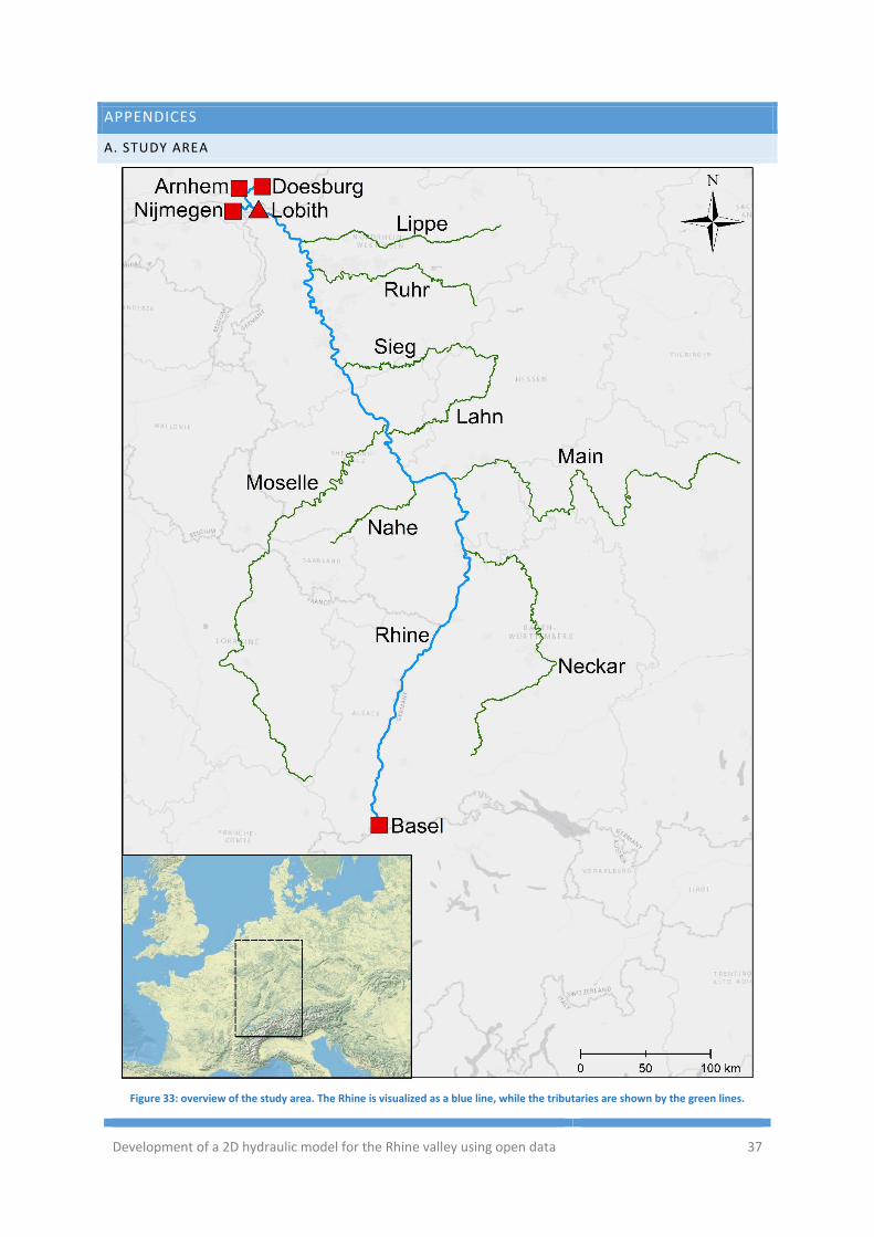
Development of a 2D hydraulic model for the Rhine valley using open data 37
APPENDICES
A. STUDY AREA
Figure 33: overview of the study area. The Rhine is visualized as a blue line, while the tributaries are shown by the green lines.
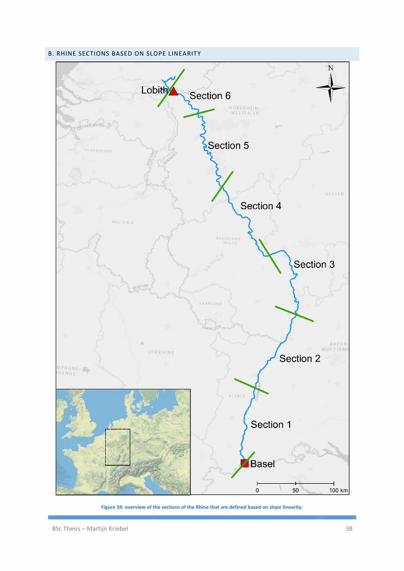
BSc Thesis – Martijn Kriebel 38
B. RHINE SECTIONS BASED ON SLOPE LINEARITY
Figure 34: overview of the sections of the Rhine that are defined based on slope linearity.
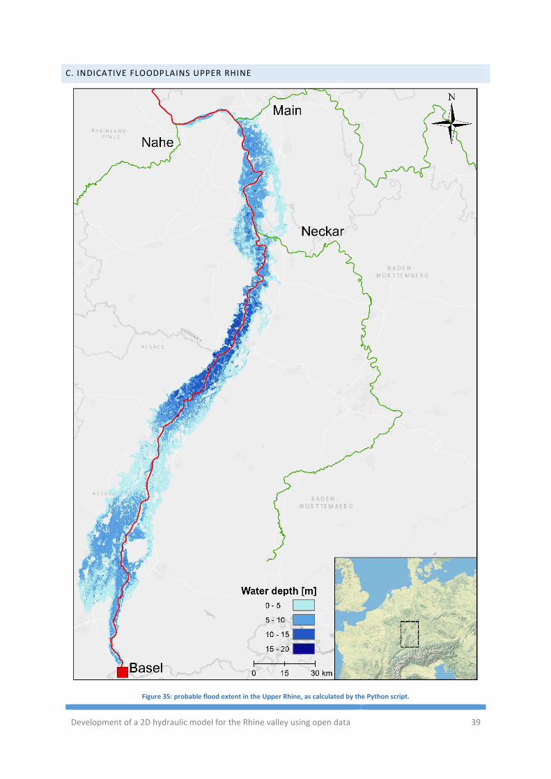
Development of a 2D hydraulic model for the Rhine valley using open data 39
C. INDICATIVE FLOODPLAINS UPPER RHINE
Figure 35: probable flood extent in the Upper Rhine, as calculated by the Python script.
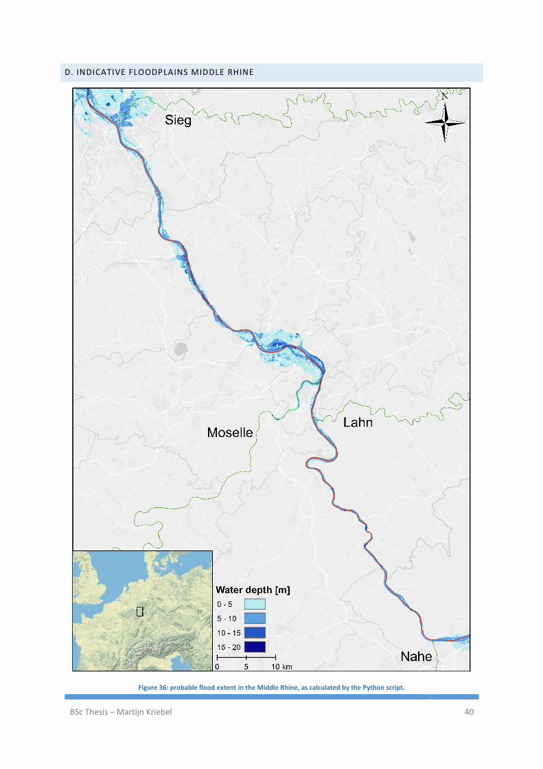
BSc Thesis – Martijn Kriebel 40
D. INDICATIVE FLOODPLAINS MIDDLE RHINE
Figure 36: probable flood extent in the Middle Rhine, as calculated by the Python script.
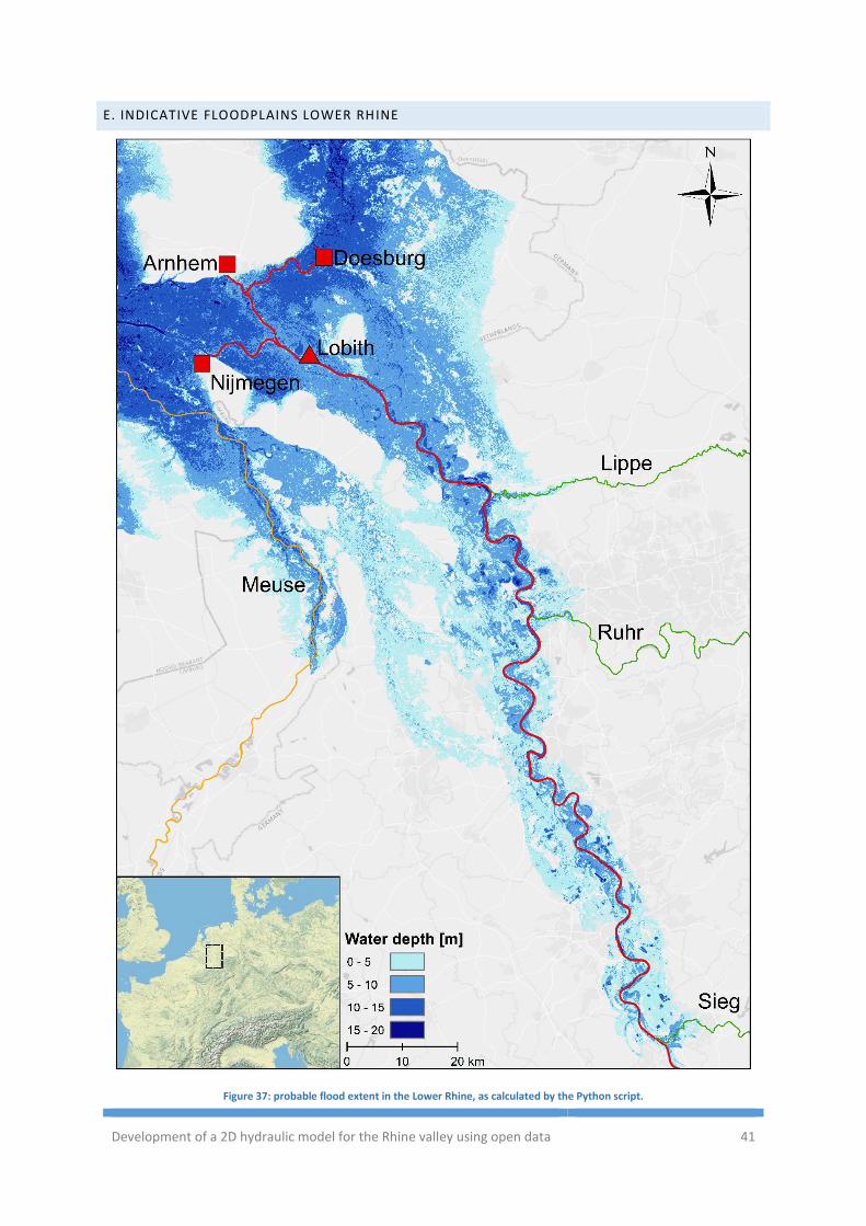
Development of a 2D hydraulic model for the Rhine valley using open data 41
E. INDICATIVE FLOODPLAINS LOWER RHINE
Figure 37: probable flood extent in the Lower Rhine, as calculated by the Python script.
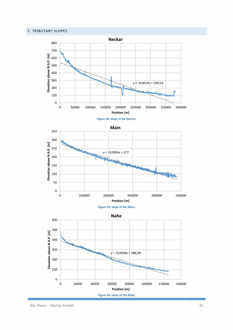
BSc Thesis – Martijn Kriebel 42
F. TRIBUTARY SLOPES
Figure 38: slope of the Neckar.
Figure 39: slope of the Main.
Figure 40: slope of the Nahe.
y = -0,0014x + 539,54
0
100
200
300
400
500
600
700
800
0 50000 100000 150000 200000 250000 300000 350000 400000
Ele
vati
on
ab
ove
N.A
.P.
[m]
Position [m]
Neckar
y = -0,0004x + 277
0
50
100
150
200
250
300
350
0 100000 200000 300000 400000 500000
Ele
vati
on
ab
ove
N.A
.P.
[m]
Position [m]
Main
y = -0,0028x + 388,09
0
100
200
300
400
500
600
0 20000 40000 60000 80000 100000 120000 140000
Ele
vati
on
ab
ove
N.A
.P.
[m]
Position [m]
Nahe
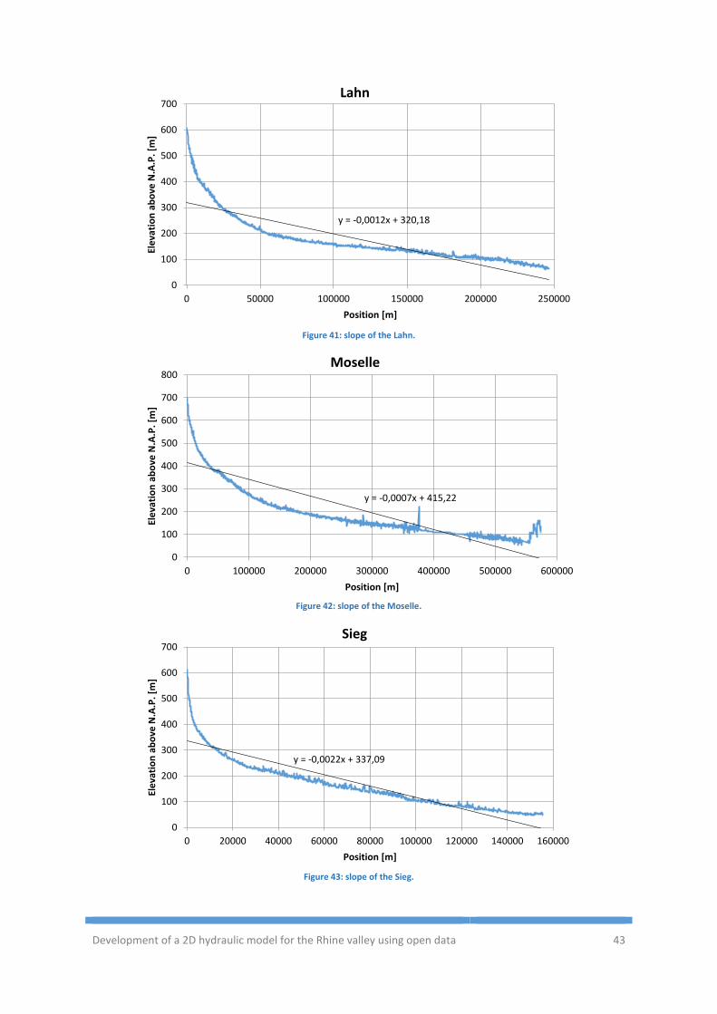
Development of a 2D hydraulic model for the Rhine valley using open data 43
Figure 41: slope of the Lahn.
Figure 42: slope of the Moselle.
Figure 43: slope of the Sieg.
y = -0,0012x + 320,18
0
100
200
300
400
500
600
700
0 50000 100000 150000 200000 250000
Ele
vati
on
ab
ove
N.A
.P.
[m]
Position [m]
Lahn
y = -0,0007x + 415,22
0
100
200
300
400
500
600
700
800
0 100000 200000 300000 400000 500000 600000
Ele
vati
on
ab
ove
N.A
.P.
[m]
Position [m]
Moselle
y = -0,0022x + 337,09
0
100
200
300
400
500
600
700
0 20000 40000 60000 80000 100000 120000 140000 160000
Ele
vati
on
ab
ove
N.A
.P.
[m]
Position [m]
Sieg
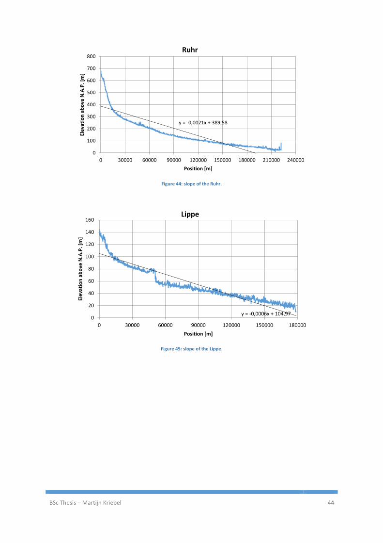
BSc Thesis – Martijn Kriebel 44
Figure 44: slope of the Ruhr.
Figure 45: slope of the Lippe.
y = -0,0021x + 389,58
0
100
200
300
400
500
600
700
800
0 30000 60000 90000 120000 150000 180000 210000 240000
Ele
vati
on
ab
ove
N.A
.P.
[m]
Position [m]
Ruhr
y = -0,0006x + 104,970
20
40
60
80
100
120
140
160
0 30000 60000 90000 120000 150000 180000
Ele
vati
on
ab
ove
N.A
.P.
[m]
Position [m]
Lippe
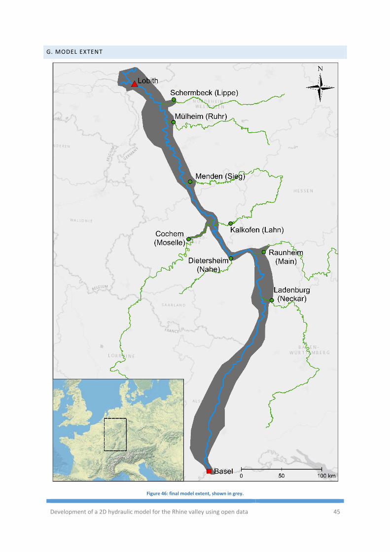
Development of a 2D hydraulic model for the Rhine valley using open data 45
G. MODEL EXTENT
Figure 46: final model extent, shown in grey.

BSc Thesis – Martijn Kriebel 46
H. ORTHOGONALITY OF COARSE GRID
Figure 47: orthogonality of the coarse grid.
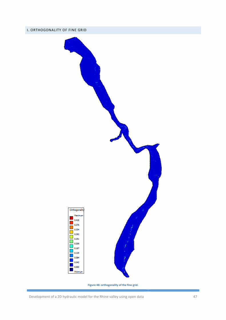
Development of a 2D hydraulic model for the Rhine valley using open data 47
I. ORTHOGONALITY OF FINE GRID
Figure 48: orthogonality of the fine grid.
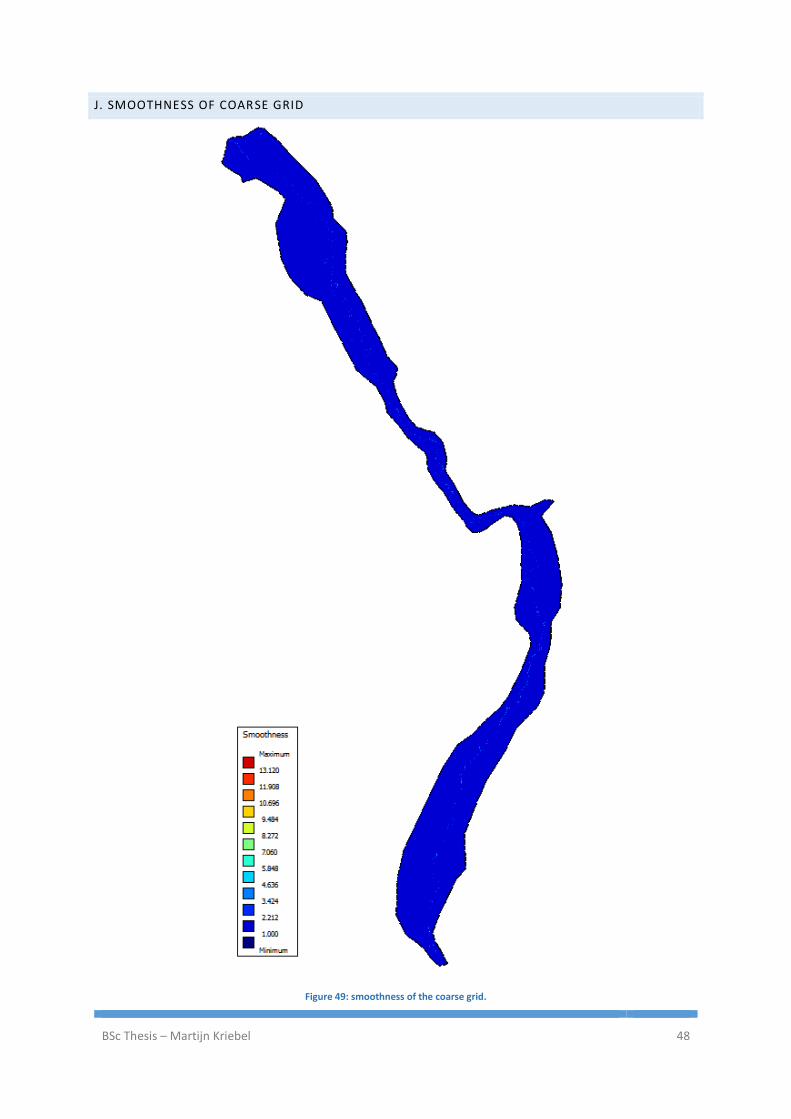
BSc Thesis – Martijn Kriebel 48
J. SMOOTHNESS OF COARSE GRID
Figure 49: smoothness of the coarse grid.

Development of a 2D hydraulic model for the Rhine valley using open data 49
K. SMOOTHNESS OF FINE GRID
Figure 50: smoothness of the fine grid.
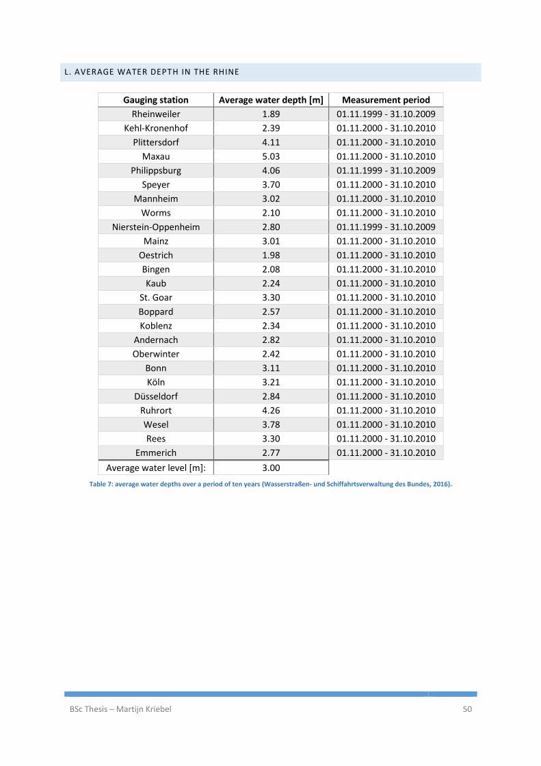
BSc Thesis – Martijn Kriebel 50
L. AVERAGE WATER DEPTH IN THE RHINE
Gauging station Average water depth [m] Measurement period
Rheinweiler 1.89 01.11.1999 - 31.10.2009
Kehl-Kronenhof 2.39 01.11.2000 - 31.10.2010
Plittersdorf 4.11 01.11.2000 - 31.10.2010
Maxau 5.03 01.11.2000 - 31.10.2010
Philippsburg 4.06 01.11.1999 - 31.10.2009
Speyer 3.70 01.11.2000 - 31.10.2010
Mannheim 3.02 01.11.2000 - 31.10.2010
Worms 2.10 01.11.2000 - 31.10.2010
Nierstein-Oppenheim 2.80 01.11.1999 - 31.10.2009
Mainz 3.01 01.11.2000 - 31.10.2010
Oestrich 1.98 01.11.2000 - 31.10.2010
Bingen 2.08 01.11.2000 - 31.10.2010
Kaub 2.24 01.11.2000 - 31.10.2010
St. Goar 3.30 01.11.2000 - 31.10.2010
Boppard 2.57 01.11.2000 - 31.10.2010
Koblenz 2.34 01.11.2000 - 31.10.2010
Andernach 2.82 01.11.2000 - 31.10.2010
Oberwinter 2.42 01.11.2000 - 31.10.2010
Bonn 3.11 01.11.2000 - 31.10.2010
Köln 3.21 01.11.2000 - 31.10.2010
Düsseldorf 2.84 01.11.2000 - 31.10.2010
Ruhrort 4.26 01.11.2000 - 31.10.2010
Wesel 3.78 01.11.2000 - 31.10.2010
Rees 3.30 01.11.2000 - 31.10.2010
Emmerich 2.77 01.11.2000 - 31.10.2010
Average water level [m]: 3.00
Table 7: average water depths over a period of ten years (Wasserstraßen- und Schiffahrtsverwaltung des Bundes, 2016).
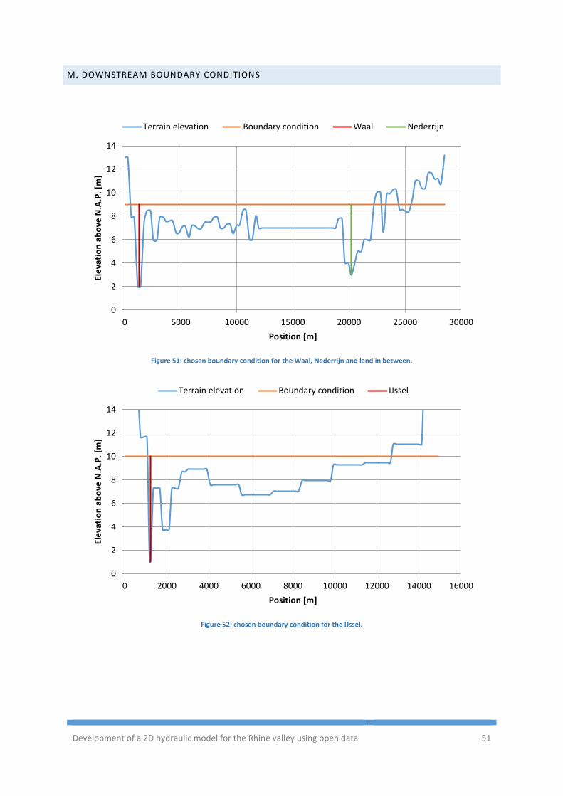
Development of a 2D hydraulic model for the Rhine valley using open data 51
M. DOWNSTREAM BOUNDARY CONDITIONS
Figure 51: chosen boundary condition for the Waal, Nederrijn and land in between.
Figure 52: chosen boundary condition for the IJssel.
0
2
4
6
8
10
12
14
0 5000 10000 15000 20000 25000 30000
Ele
vati
on
ab
ove
N.A
.P.
[m]
Position [m]
Terrain elevation Boundary condition Waal Nederrijn
0
2
4
6
8
10
12
14
0 2000 4000 6000 8000 10000 12000 14000 16000
Ele
vati
on
ab
ove
N.A
.P.
[m]
Position [m]
Terrain elevation Boundary condition IJssel
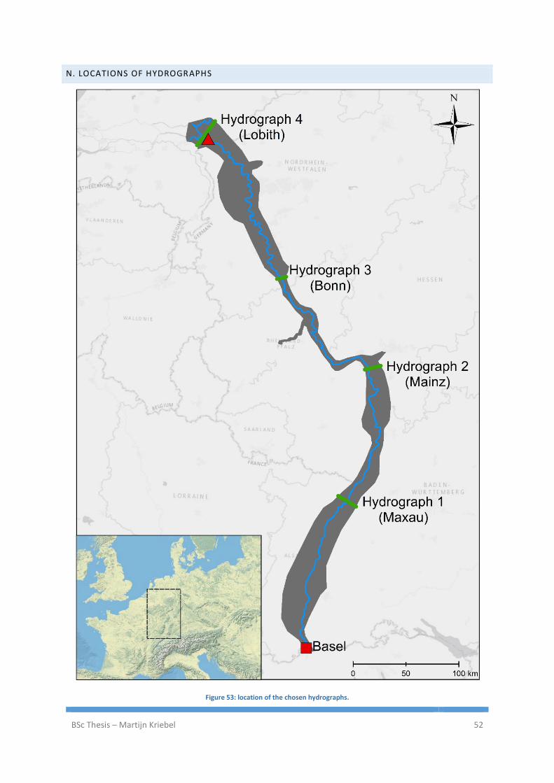
BSc Thesis – Martijn Kriebel 52
N. LOCATIONS OF HYDROGRAPHS
Figure 53: location of the chosen hydrographs.