Intro. to the Smith Chart

Transmission Line Applications

Background

• Philip Smith of Bell Laboratories developed the “Smith Chart” back in the 1930”s to expedite the tedious and repetative solution of certain rf design problems. These include:

• Transmission line problems• Rf amplifier design and analysis• L-C impedance matching networks• Plotting of antenna impedance• Etc.

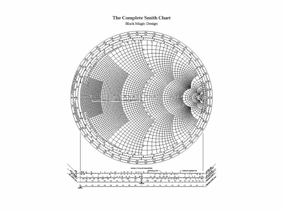
CONSTRUCTION

• The Smith Chart is made up of a family of circles and a second family of arcs of circles.

• The circles are called “constant resistance circles”• The arcs are “constant reactance circles”• Impedances must be entered in rectangular form –

broken down into a real and an imaginary component.• The real part (resistance) determines the circle to use.• The imaginary part (reactance) determines the arc to

use.• The intersection of an arc and a circle represents the

plotted impedance.

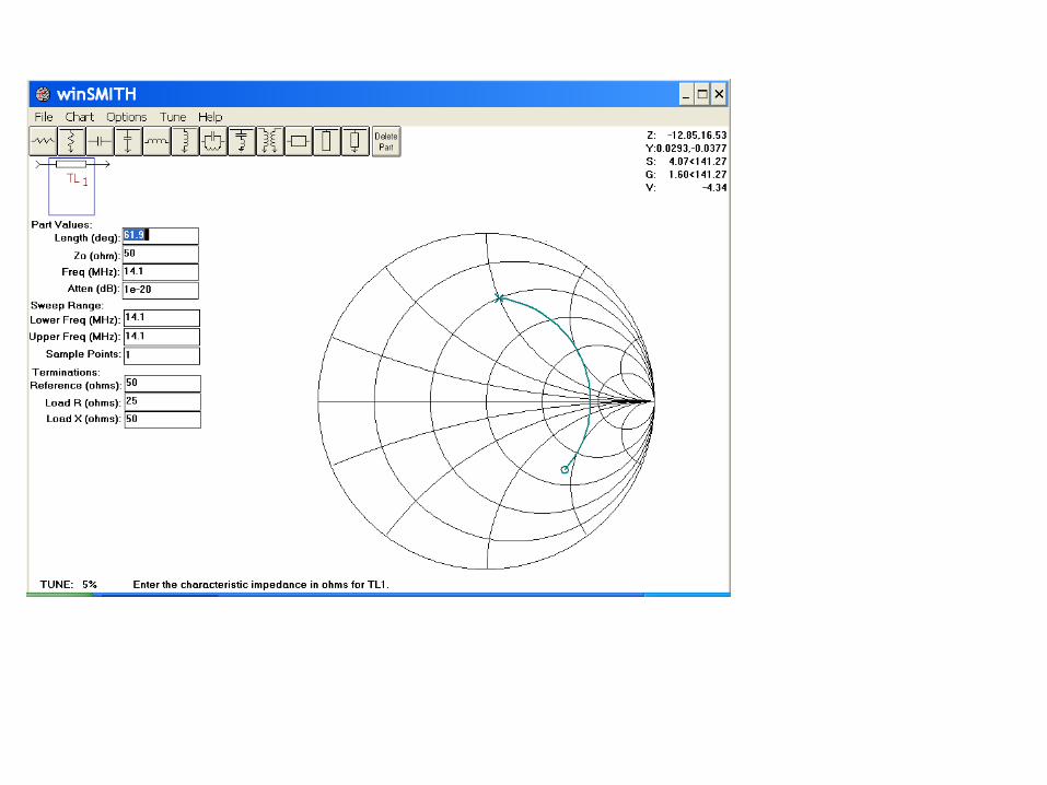
Antenna Z known, find Z at transmitter___________________________________________________________________ Assume an antenna impedance (ZL ) of 25 + j50 ohms

Let characteristic impedance of the transmission line = 50 ohms

Let velocity factor of cable (vf) = 0.66

Let physical line length = 100 feet = 30.48 meters

Let the frequency (f) be 14.1 MHz___________________________________________________________________One electrical wavelength on cable = (983.6)(vf)/f(MHz) = (983.6)(.66)/14.1 = 46.04 ft.

Wavelength of actual cable = 100 ft./46.04 ft. = 2.172 wavelengths or 781.9 degrees

Subtract 0.5 wavelengths until the result is less than or equal to 0.5 wavelengths.

The length to plot is 0.172 wavelengths or 61.9° (toward source).

Normalize Load Z

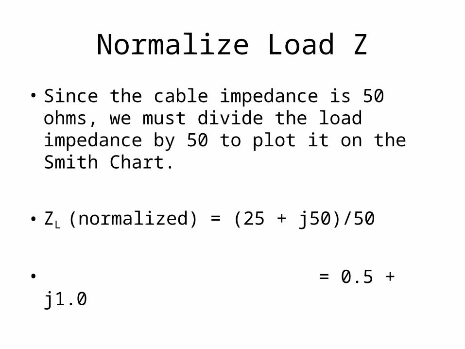
• Since the cable impedance is 50 ohms, we must divide the load impedance by 50 to plot it on the Smith Chart.

• ZL (normalized) = (25 + j50)/50

• = 0.5 + j1.0

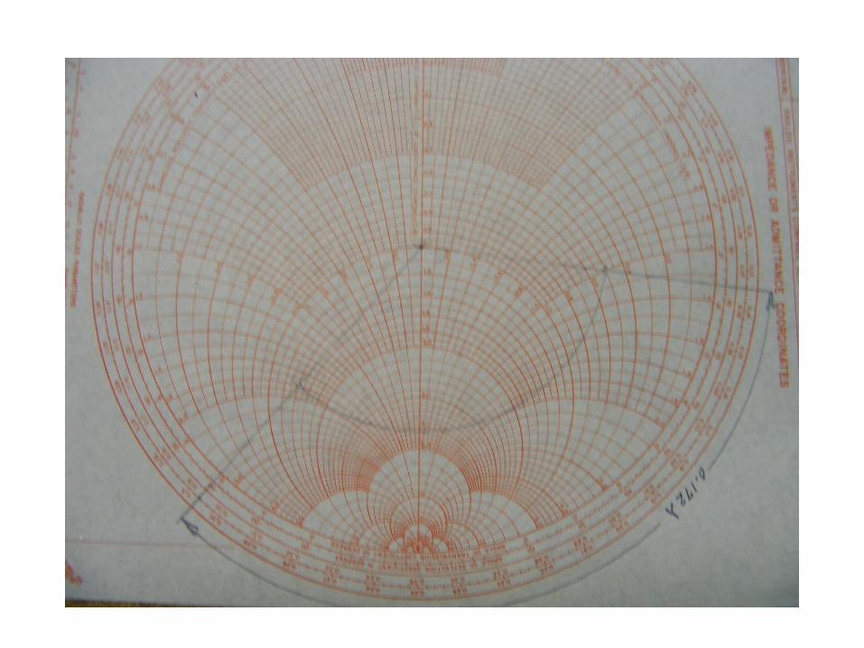
Plotting

• Place a dot at 0.5+ J1.0• Extend a radial line from the center through 0.5+j1.0 to the “wavelengths

toward generator” scale on the periphery.• Read approx. 0.1345 • Add 0.172 to get 0.3065• Extend another radial line from the center

through 0.3065 on the “wavelengths toward generator” scale.

Plotting Cont’

• Place one leg of your dividers on the center and the other leg on 0.5+j1.0

• Draw an arc clockwise (0.172 wavelengths) to the second radial.

• Read approx. 1.4 – j1.8 at the intersection.• Multiple by 50 to un-normalize.• Z at sending end is approx. 70-j90 ohms (An inductive antenna impedance looks

capacitive at the transmitter.)

FCG 12-26-09

OHMSZin 68.766 90.794iAnswer:

________________________________________________________________________________________

Zin Zo

ZL

Zo

cos j sin

cos jZL

Zo

sin

________________________________________________________________________________________

ZL 25 50j

Zo 50

61.9deg

l 100ft

Problem parameters:

______________________________________________________________________________________define "j"j 1

______________________________________________________________________________________

Input Impedance (Zin) of a lossless transmission line :