INNOVATIVE DISPERSION MODELING PRACTICES TO ACHIEVE A REASONABLE LEVEL OF CONSERVATISM IN AERMODMODELING DEMONSTRATIONSCASE STUDY TO EVALUATE EMVAP, AMR2, AND BACKGROUND CONCENTRATIONS

Presentation to the Board of the Upper Midwest Section of the Air & Waste Management Association

September 16, 2014

Sergio A. Guerra - Wenck Associates, Inc.

Challenge of new short-term NAAQS

2

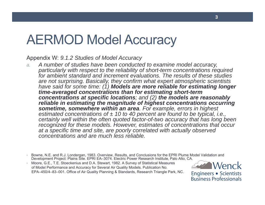
AERMOD Model AccuracyAppendix W: 9.1.2 Studies of Model Accuracy a. A number of studies have been conducted to examine model accuracy,

particularly with respect to the reliability of short-term concentrations required for ambient standard and increment evaluations. The results of these studies are not surprising. Basically, they confirm what expert atmospheric scientists have said for some time: (1) Models are more reliable for estimating longer time-averaged concentrations than for estimating short-term concentrations at specific locations; and (2) the models are reasonably reliable in estimating the magnitude of highest concentrations occurring sometime, somewhere within an area. For example, errors in highest estimated concentrations of ± 10 to 40 percent are found to be typical, i.e., certainly well within the often quoted factor-of-two accuracy that has long been recognized for these models. However, estimates of concentrations that occur at a specific time and site, are poorly correlated with actually observed concentrations and are much less reliable.

• Bowne, N.E. and R.J. Londergan, 1983. Overview, Results, and Conclusions for the EPRI Plume Model Validation and Development Project: Plains Site. EPRI EA–3074. Electric Power Research Institute, Palo Alto, CA.

• Moore, G.E., T.E. Stoeckenius and D.A. Stewart, 1982. A Survey of Statistical Measures of Model Performance and Accuracy for Several Air Quality Models. Publication No. EPA–450/4–83–001. Office of Air Quality Planning & Standards, Research Triangle Park, NC.

3

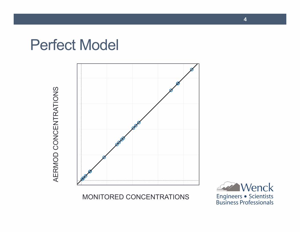
Perfect Model

4

MONITORED CONCENTRATIONS

AE

RM

OD

CO

NC

EN

TRAT

ION

S

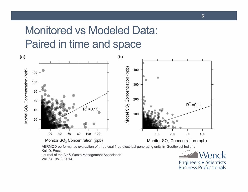
Monitored vs Modeled Data:Paired in time and space

AERMOD performance evaluation of three coal-fired electrical generating units in Southwest IndianaKali D. Frost Journal of the Air & Waste Management Association Vol. 64, Iss. 3, 2014

5

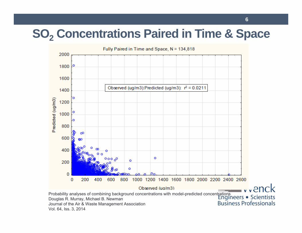
SO2 Concentrations Paired in Time & Space

Probability analyses of combining background concentrations with model-predicted concentrationsDouglas R. Murray, Michael B. Newman Journal of the Air & Waste Management Association Vol. 64, Iss. 3, 2014

6

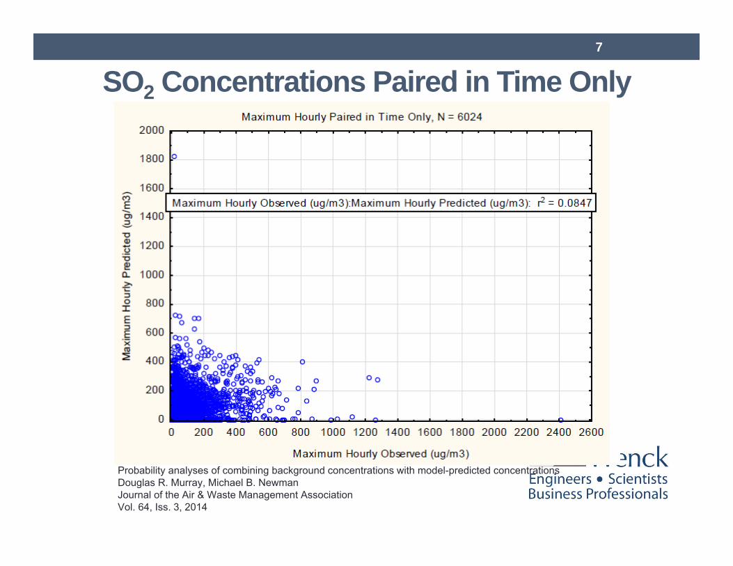
SO2 Concentrations Paired in Time Only

Probability analyses of combining background concentrations with model-predicted concentrationsDouglas R. Murray, Michael B. Newman Journal of the Air & Waste Management Association Vol. 64, Iss. 3, 2014

7

Roadmap• Case study based on 4 reciprocating internal combustion

engines (RICE) used for emergency purposes• Engines are also part of a peaking shaving agreement

and may be required to operate 250 hour per year• 3 Modeling techniques are presented

• EMVAP• ARM2• The use of the 50th percentile monitored concentration as Bkg

8

EMVAP• Problem: Currently assume continuous emissions from

proposed project or modification• In this case study an applicant is requesting to load shave

250 hour per year.• Current modeling practices prescribe that the engines be

modeled as if in continuous operation(i.e., 8760 hour/year).

• EMVAP assigns emission rates at random over numerous iterations.

• The resulting distribution from EMVAP yields a more representative approximation of actual impacts

9

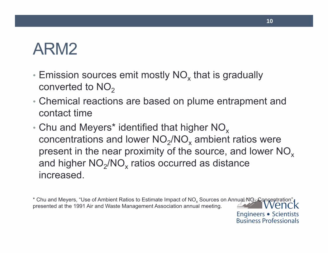
ARM2• Emission sources emit mostly NOx that is gradually

converted to NO2

• Chemical reactions are based on plume entrapment and contact time

• Chu and Meyers* identified that higher NOxconcentrations and lower NO2/NOx ambient ratios were present in the near proximity of the source, and lower NOxand higher NO2/NOx ratios occurred as distance increased.

* Chu and Meyers, “Use of Ambient Ratios to Estimate Impact of NOx Sources on Annual NO2 Concentration”, presented at the 1991 Air and Waste Management Association annual meeting.

10

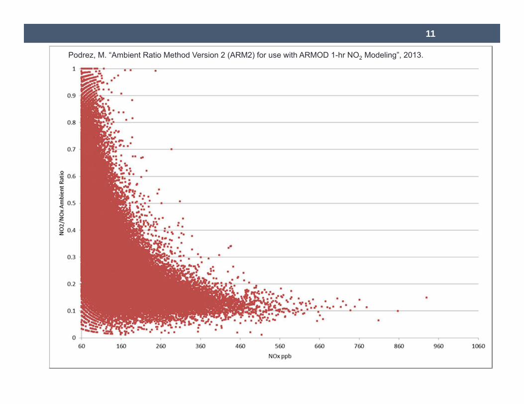
Podrez, M. “Ambient Ratio Method Version 2 (ARM2) for use with ARMOD 1-hr NO2 Modeling”, 2013.

11

Four cases evaluatedInput parameter Case 1 Case 2 Case 3 Case 4

Description of Dispersion Modeling

Current Modeling Practices

EMVAP(500 iterations)

ARM2 MethodEMVAP and

ARM2 Method

Maximum peak shaving hours per

year250 250 250 250

Hours of operation assigned in the

model8760 250 8760 250

NOx to NO2

Conversion

Assumed 100%

conversion

Assumed 100% conversion

Calculated based on the ARM2

equation

Calculated based on the ARM2

equation

12

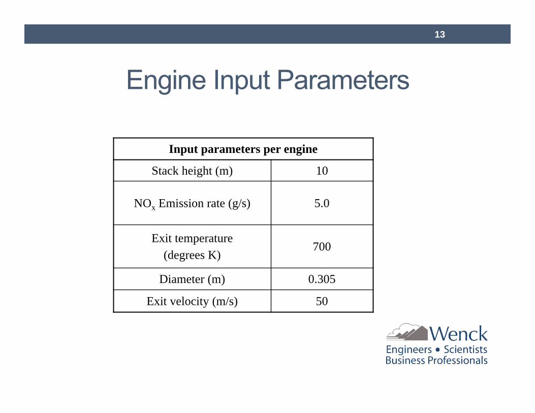
Engine Input Parameters

Input parameters per engine

Stack height (m) 10

NOx Emission rate (g/s) 5.0

Exit temperature(degrees K)

700

Diameter (m) 0.305

Exit velocity (m/s) 50

13

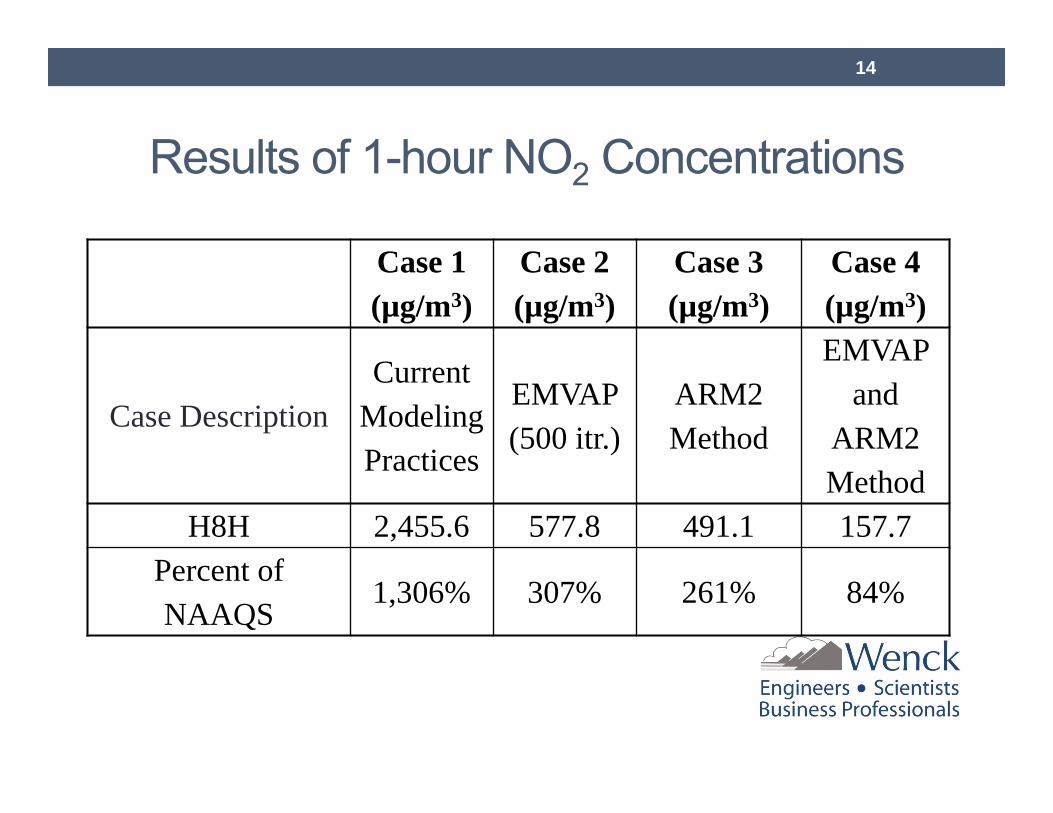
Results of 1-hour NO2 Concentrations

Case 1 (µg/m3)

Case 2 (µg/m3)

Case 3 (µg/m3)

Case 4 (µg/m3)

Case DescriptionCurrent

Modeling Practices

EMVAP(500 itr.)

ARM2Method

EMVAPand

ARM2Method

H8H 2,455.6 577.8 491.1 157.7Percent of NAAQS

1,306% 307% 261% 84%

14

Background Concentrations

15

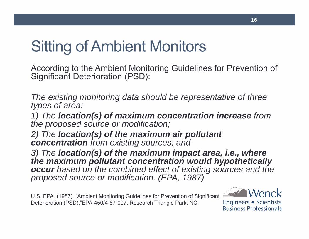
Sitting of Ambient MonitorsAccording to the Ambient Monitoring Guidelines for Prevention of Significant Deterioration (PSD):

The existing monitoring data should be representative of three types of area:1) The location(s) of maximum concentration increase from the proposed source or modification;2) The location(s) of the maximum air pollutant concentration from existing sources; and3) The location(s) of the maximum impact area, i.e., where the maximum pollutant concentration would hypothetically occur based on the combined effect of existing sources and the proposed source or modification. (EPA, 1987)

U.S. EPA. (1987). “Ambient Monitoring Guidelines for Prevention of Significant Deterioration (PSD).”EPA‐450/4‐87‐007, Research Triangle Park, NC.

16

Exceptional Events

http://blogs.mprnews.org/updraft/2012/06/co_smoke_plume_now_visible_abo/

17

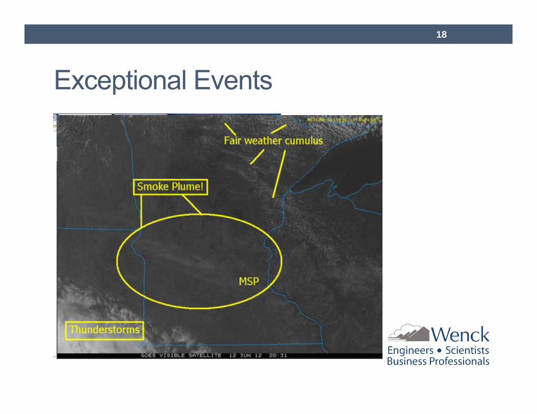
Exceptional Events

18

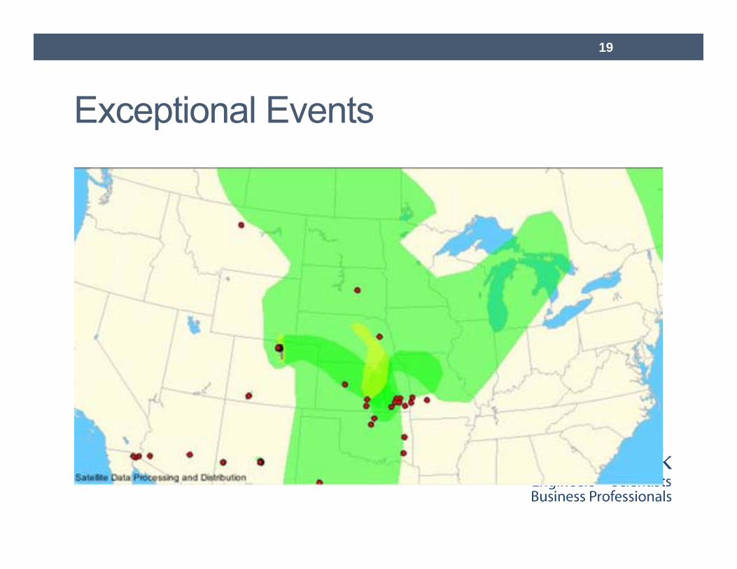
Exceptional Events

19

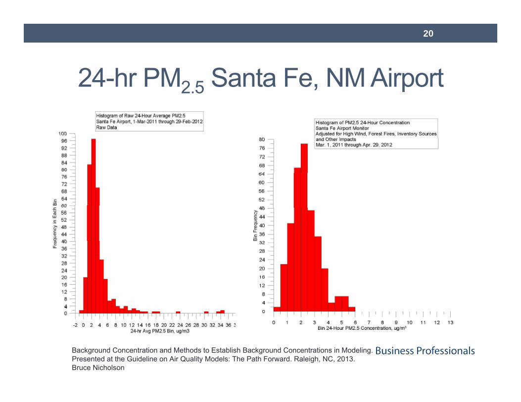
24-hr PM2.5 Santa Fe, NM Airport

Background Concentration and Methods to Establish Background Concentrations in Modeling. Presented at the Guideline on Air Quality Models: The Path Forward. Raleigh, NC, 2013.Bruce Nicholson

20

Probability of two unusual events

21

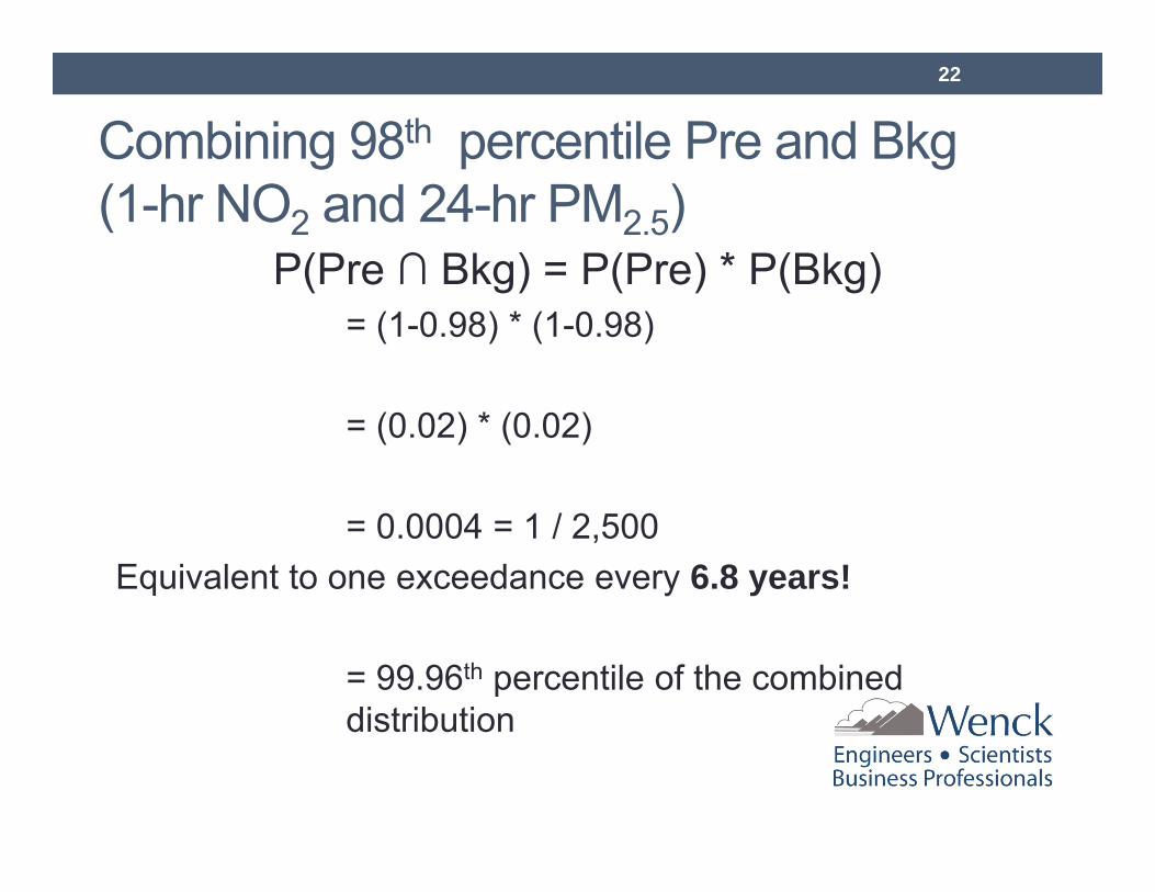
Combining 98th percentile Pre and Bkg (1-hr NO2 and 24-hr PM2.5)

P(Pre ∩ Bkg) = P(Pre) * P(Bkg)= (1-0.98) * (1-0.98)

= (0.02) * (0.02)

= 0.0004 = 1 / 2,500Equivalent to one exceedance every 6.8 years!

= 99.96th percentile of the combined distribution

22

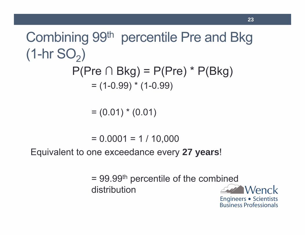
Combining 99th percentile Pre and Bkg (1-hr SO2)

P(Pre ∩ Bkg) = P(Pre) * P(Bkg)= (1-0.99) * (1-0.99)

= (0.01) * (0.01)

= 0.0001 = 1 / 10,000Equivalent to one exceedance every 27 years!

= 99.99th percentile of the combined distribution

23

Proposed Approach to Combine Modeled and Monitored Concentrations• Combining the 98th (or 99th for 1-hr SO2) % monitored

concentration with the 98th % predicted concentration is too conservative.

• A more reasonable approach is to use a monitored value closer to the main distribution (i.e., the median).

Evaluation of the SO2 and NOX offset ratio method to account for secondary PM2.5 formationSergio A. Guerra, Shannon R. Olsen, Jared J. Anderson Journal of the Air & Waste Management Association Vol. 64, Iss. 3, 2014

24

Combining 98th Pre and 50th Bkg P(Pre ∩ Bkg) = P(Pre) * P(Bkg)

= (1-0.98) * (1-0.50)

= (0.02) * (0.50)

= 0.01 = 1 / 100

= 99th percentile of the combined distribution

Evaluation of the SO2 and NOX offset ratio method to account for secondary PM2.5 formationSergio A. Guerra, Shannon R. Olsen, Jared J. Anderson Journal of the Air & Waste Management Association Vol. 64, Iss. 3, 2014

25

Combining 99th Pre and 50th Bkg P(Pre ∩ Bkg) = P(Pre) * P(Bkg)

= (1-0.99) * (1-0.50)

= (0.01) * (0.50)

= 0.005 = 1 / 200

= 99.5th percentile of the combined distribution

Evaluation of the SO2 and NOX offset ratio method to account for secondary PM2.5 formationSergio A. Guerra, Shannon R. Olsen, Jared J. Anderson Journal of the Air & Waste Management Association Vol. 64, Iss. 3, 2014

26

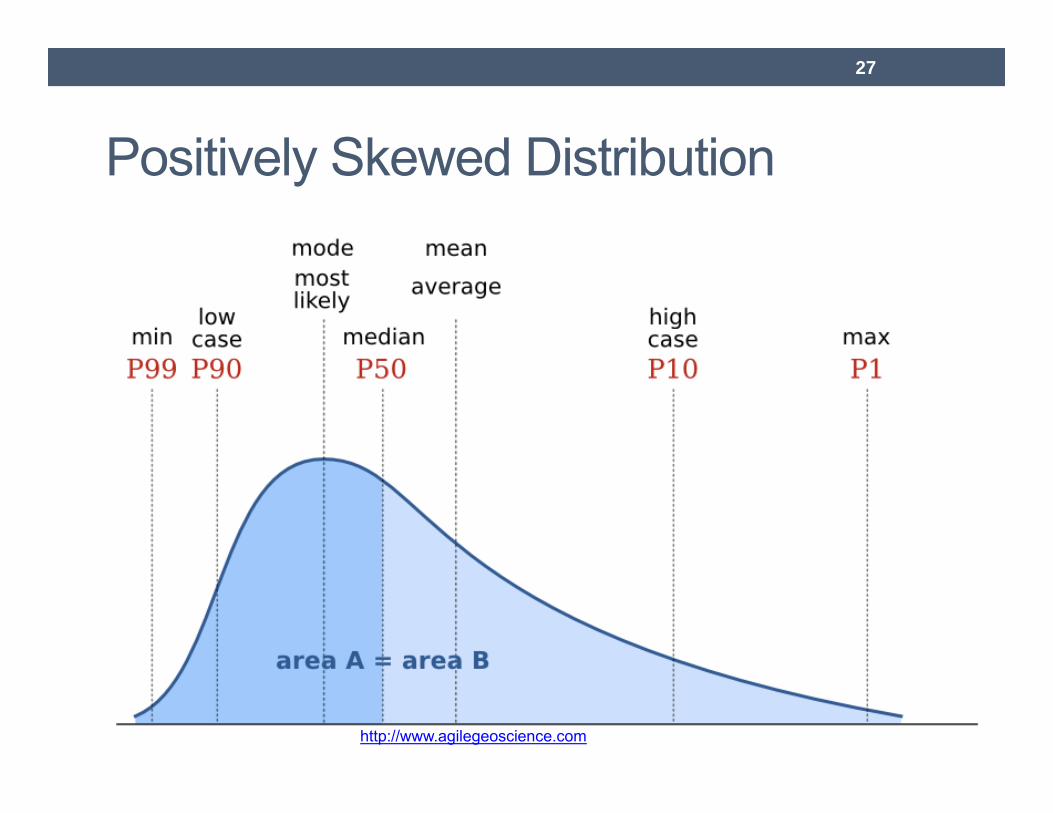
Positively Skewed Distribution

http://www.agilegeoscience.com

27

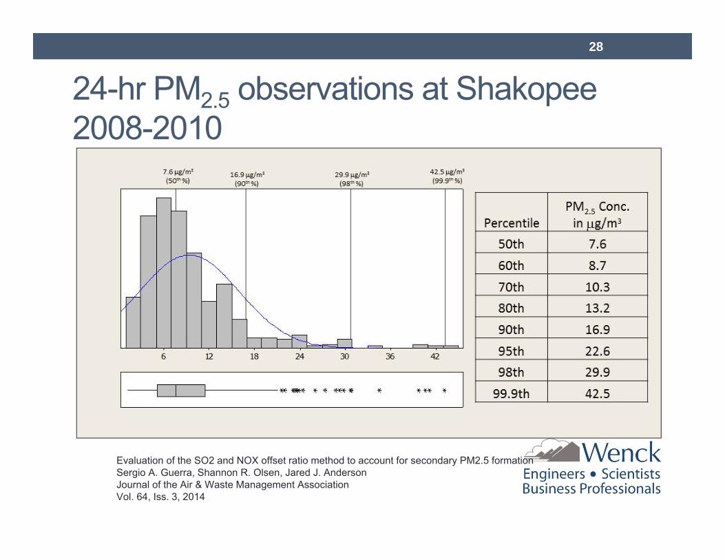
24-hr PM2.5 observations at Shakopee 2008-2010

Evaluation of the SO2 and NOX offset ratio method to account for secondary PM2.5 formationSergio A. Guerra, Shannon R. Olsen, Jared J. Anderson Journal of the Air & Waste Management Association Vol. 64, Iss. 3, 2014

28

Background concentrations1) Bkg 1: Maximum 1-hour NO2 observations from the

Blaine monitor averaged over three years.2) Bkg 2: Average of the annual 98th percentile daily

maximum 1-hour NO2 concentrations for years 2010-2012.

3) Bkg 3: 50th percentile concentration from the 2010-2012 hourly observations.

29

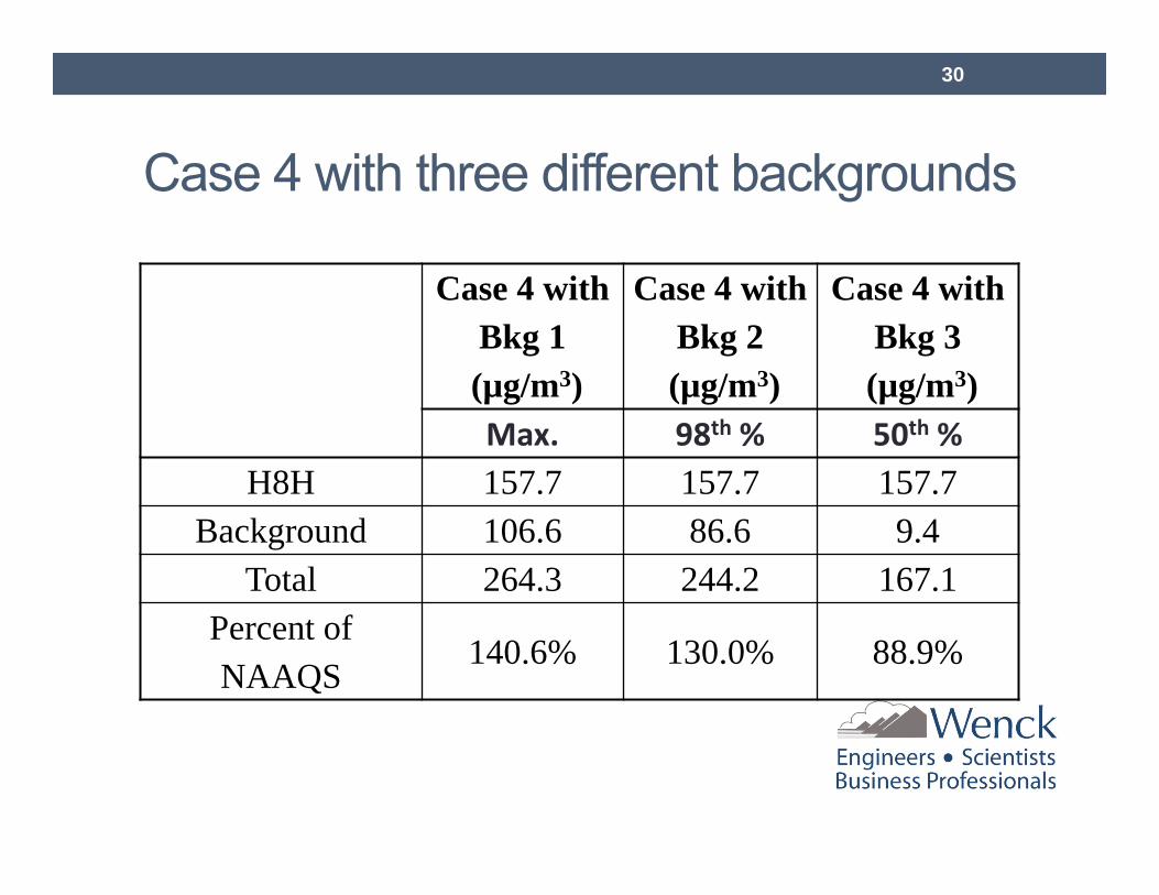
Case 4 with three different backgrounds

Case 4 with Bkg 1(µg/m3)

Case 4 with Bkg 2(µg/m3)

Case 4 with Bkg 3(µg/m3)

Max. 98th % 50th %H8H 157.7 157.7 157.7

Background 106.6 86.6 9.4Total 264.3 244.2 167.1

Percent of NAAQS

140.6% 130.0% 88.9%

30

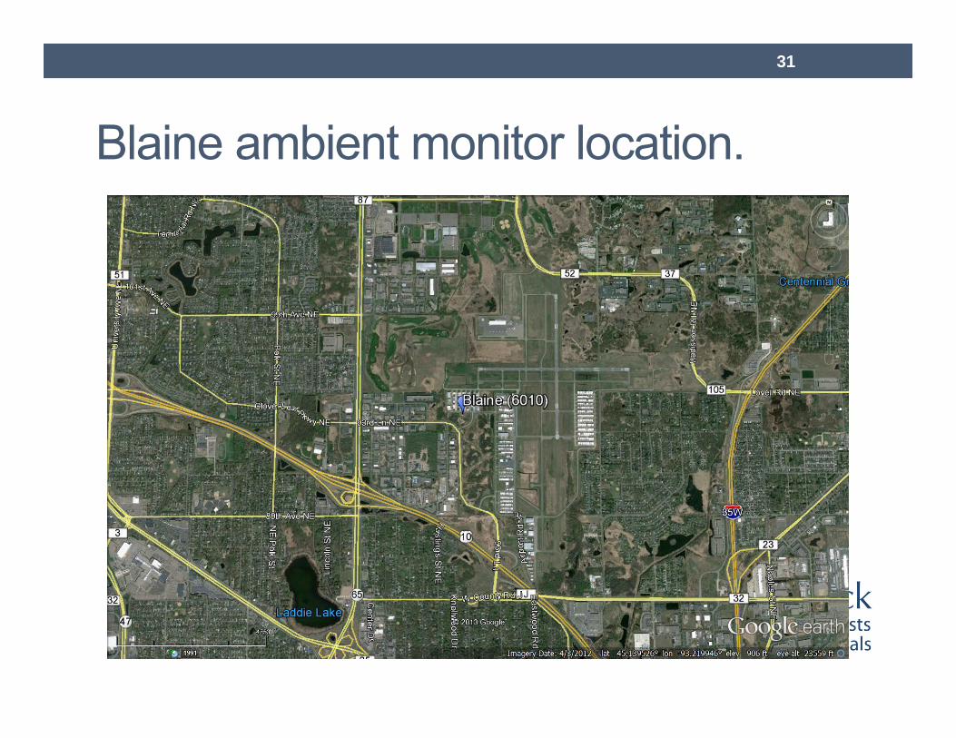
Blaine ambient monitor location.

31

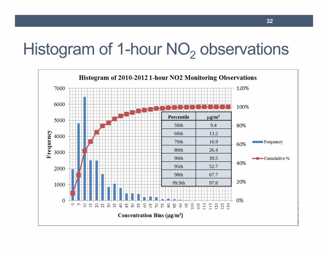
Histogram of 1-hour NO2 observations

Percentile g/m3

50th 9.4

60th 13.2

70th 16.9

80th 26.4

90th 39.5

95th 52.7

98th 67.7

99.9th 97.8

32

Conclusion• Use of EMVAP and ARM2 can help achieve more realistic concentrations

• Use of 50th % monitored concentration is statistically conservative when pairing it with the 98th (or 99th) % predicted concentration

• 3 Methods are protective of the NAAQS while still providing a reasonable level of conservatism

33

QUESTIONS…

Sergio A. Guerra, PhDEnvironmental EngineerPhone: (952) 837-3340sguerra@wenck.com

www.SergioAGuerra.com

34