Embed Size (px)
Citation preview
Technical Introduction to Geostationary Satellite Communication Systems Original Prepared by Telesat Canada
Slide Number 1Rev -, July 2001
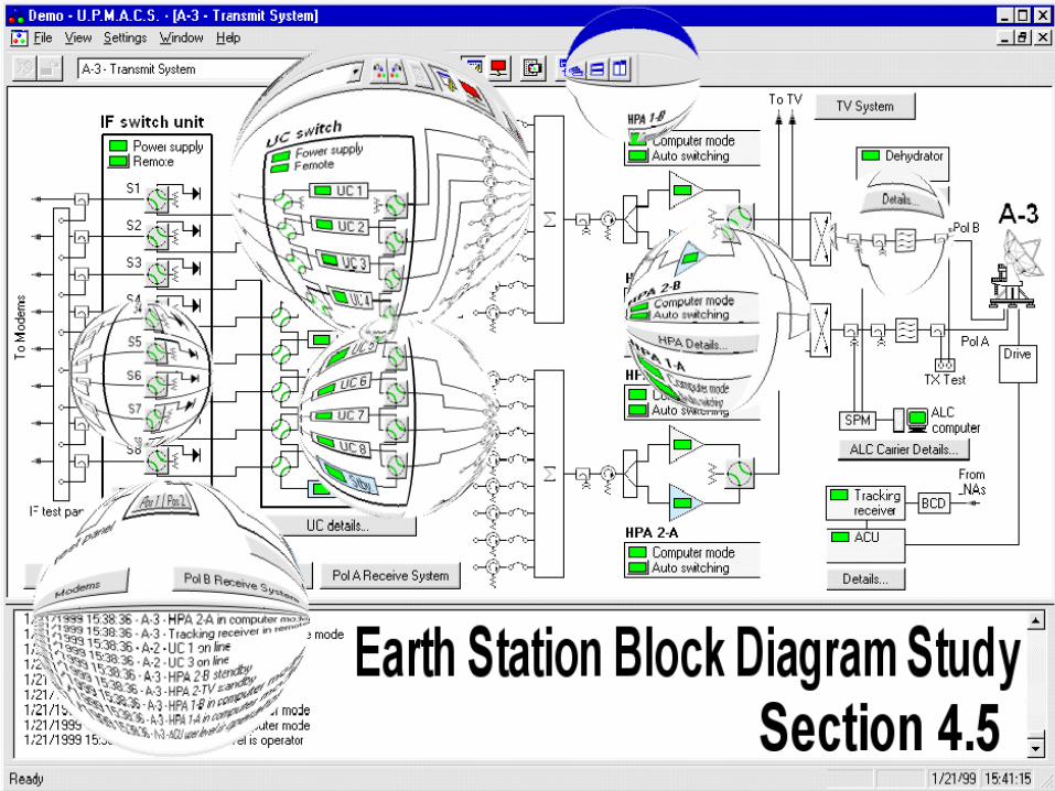
Earth Station Block Diagram Study
Section 5
Vol 4: Earth Stations
Technical Introduction to Geostationary Satellite Communication Systems Original Prepared by Telesat Canada
Slide Number 2Rev -, July 2001
Contents4.5.1 Block & Level Diagram Introduction4.5.2 Antenna Subsystem4.5.3 Low Noise Amplifiers 4.5.4 High Power Amplifiers (HPA)4.5.5 Up & Down Conversion4.5.6 Modems4.5.7 Exciters4.5.8 Baseband Equipment4.5.9 Redundancy Equipment4.5.10 Passive Devices
4.5: Earth Station Block Diagram StudyVol 4: Earth Stations
Technical Introduction to Geostationary Satellite Communication Systems Original Prepared by Telesat Canada
Slide Number 3Rev -, July 2001
4.5: Earth Station Block Diagram StudyVol 4: Earth Stations
Block & Level Diagram IntroducedPart 1
Technical Introduction to Geostationary Satellite Communication Systems Original Prepared by Telesat Canada
Slide Number 4Rev -, July 2001
How to Read a Block & Level Diagram
Part 1: Block and Level Diagram Introduced
A block diagram is a useful tool. It depicts a simplified, high-level schematic of the interconnection of major equipment units in a communication system. It can be used to:
• Troubleshoot problems • Follow signal flow • Check for proper signal levels
A block diagram is often annotated with signal level information with respect to an impedance of 50, 75 or 600 ohms (these are the most common impedance's, but any impedance level could be referenced).
When a block diagram is so marked, it is known as a Block & Level diagram.
4.5.1.1: How To Read a Block & Level Diagram
Vol 4: Earth Stations, Sec 5: Earth Station Block Diagram Study
Technical Introduction to Geostationary Satellite Communication Systems Original Prepared by Telesat Canada
Slide Number 5Rev -, July 2001
Typically, Earth Station transmit levels are measured with a power meter or a spectrum analyzer.
For single carriers, a power meter can be used with proper measurement results. In a multi-carrier environment, the preferred tool for measurement is a spectrum analyzer.
When measurements are made with a spectrum analyzer, the measurement is not a composite level but rather a selective frequency measurement.
If a composite level is to be measured, a power meter should always be used. This applies to the measurement of both receive and transmit levels.
Part 1: Block and Level Diagram Introduced
4.5.1.1: How To Read a Block & Level Diagram
Vol 4: Earth Stations, Sec 5: Earth Station Block Diagram Study
How to Read a Block & Level Diagram
Technical Introduction to Geostationary Satellite Communication Systems Original Prepared by Telesat Canada
Slide Number 6Rev -, July 2001
Some block and level diagrams include footnotes for specific measurements. These footnotes will give specific information about that measurement.
It may be stated whether the measurement is a composite or not. If not, it is common—and very useful—to include the spectrum analyzer resolution bandwidth setting used to produce the given measured value.
In reading and using block and level diagrams, care must always be taken to determine whether the listed value represents a composite or selective level. Incorrect level settings can cause equipment malfunction or the inordinate generation of C/I product.
In addition, levels are always referenced to a specific impedance, and care must be taken to ensure that measurement sets are configured to use that impedance.
Part 1: Block and Level Diagram Introduced
4.5.1.1: How To Read a Block & Level Diagram
Vol 4: Earth Stations, Sec 5: Earth Station Block Diagram Study
How to Read a Block & Level Diagram
Technical Introduction to Geostationary Satellite Communication Systems Original Prepared by Telesat Canada
Slide Number 7Rev -, July 2001
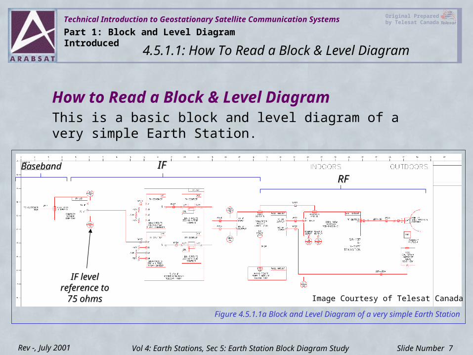
This is a basic block and level diagram of a very simple Earth Station.
IFIFRFRF
BasebandBaseband
IF level IF level reference to reference to
75 ohms75 ohms
Part 1: Block and Level Diagram Introduced
4.5.1.1: How To Read a Block & Level Diagram
Vol 4: Earth Stations, Sec 5: Earth Station Block Diagram Study
Image Courtesy of Telesat CanadaFigure 4.5.1.1a Block and Level Diagram of a very simple Earth Station
How to Read a Block & Level Diagram
Technical Introduction to Geostationary Satellite Communication Systems Original Prepared by Telesat Canada
Slide Number 8Rev -, July 2001
Signal FlowThe standard practice in depiction of signal flow is to go from the baseband signal level (demarcation point) at the left side of the page or drawing to the Earth Station antenna at the far right side of the drawing.
Signal flow progresses from Baseband, to IF (Intermediate Frequencies) to RF (Radio Frequencies) to the antenna for the transmission and reception of satellite frequencies.
Part 1: Block and Level Diagram Introduced
4.5.1.2: Signal Flow
Vol 4: Earth Stations, Sec 5: Earth Station Block Diagram Study
Technical Introduction to Geostationary Satellite Communication Systems Original Prepared by Telesat Canada
Slide Number 9Rev -, July 2001
4.5: Earth Station Block Diagram StudyVol 4: Earth Stations
Antenna SubsystemsPart 2
Technical Introduction to Geostationary Satellite Communication Systems Original Prepared by Telesat Canada
Slide Number 10Rev -, July 2001
Contents
Sec 5: Earth Stations Block Diagram Study
4.5.2.1 Types of Antennas4.5.2.2 Feeds4.5.2.3 Antenna Characteristics4.5.2.4 Antenna Structures (Mount & Foundation)4.5.2.5 Tracking Systems4.5.2.6 Three axis stabilized systems4.5.2.7 De-icing Equipment
4.5.2: Antenna Subsystems
Vol 4: Earth Stations
Technical Introduction to Geostationary Satellite Communication Systems Original Prepared by Telesat Canada
Slide Number 11Rev -, July 2001
Types of Antennas
Part 2: Antenna Subsystem
Types of antennas are:
• Prime Focus
• Cassegrain
• Gregorian
• Offset
• Dual Offset
• Receive Only
4.5.2.1: Types of Antennas
Vol 4: Earth Stations, Sec 5: Earth Station Block Diagram Study
Technical Introduction to Geostationary Satellite Communication Systems Original Prepared by Telesat Canada
Slide Number 12Rev -, July 2001
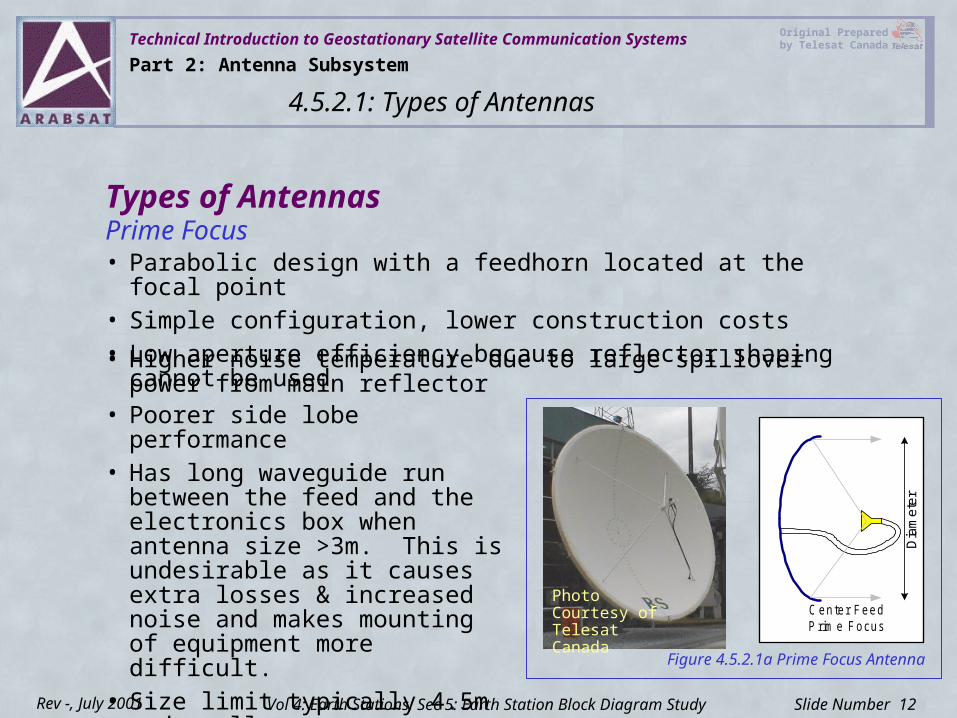
Types of AntennasPrime Focus• Parabolic design with a feedhorn located at the focal point• Simple configuration, lower construction costs• Low aperture efficiency because reflector shaping cannot be used
Dia
met
er
Center FeedP rim e Focus
Part 2: Antenna Subsystem
4.5.2.1: Types of Antennas
Vol 4: Earth Stations, Sec 5: Earth Station Block Diagram Study
• Higher noise temperature due to large spillover power from main reflector
• Poorer side lobe performance• Has long waveguide run between
the feed and the electronics box when antenna size >3m. This is undesirable as it causes extra losses & increased noise and makes mounting of equipment more difficult.
• Size limit typically 4.5m and smallerFigure 4.5.2.1a Prime Focus Antenna
Photo Courtesy of Telesat Canada
Technical Introduction to Geostationary Satellite Communication Systems Original Prepared by Telesat Canada
Slide Number 13Rev -, July 2001
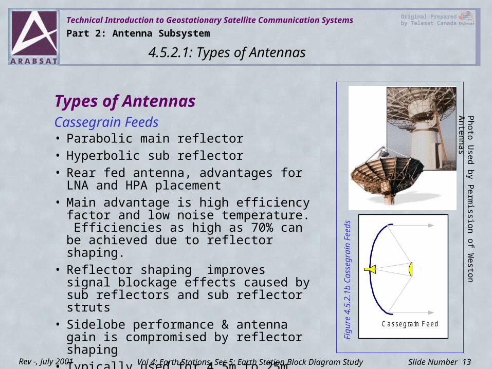
Types of AntennasCassegrain Feeds• Parabolic main reflector• Hyperbolic sub reflector • Rear fed antenna, advantages for LNA and
HPA placement• Main advantage is high efficiency factor and
low noise temperature. Efficiencies as high as 70% can be achieved due to reflector shaping.
• Reflector shaping improves signal blockage effects caused by sub reflectors and sub reflector struts
• Sidelobe performance & antenna gain is compromised by reflector shaping
• Typically used for 4.5m to 25m antennas Cassegra in Feed
Part 2: Antenna Subsystem
4.5.2.1: Types of Antennas
Vol 4: Earth Stations, Sec 5: Earth Station Block Diagram Study
Figu
re 4
.5.2
.1b
Cas
segr
ain
Feed
s
Photo Used by Permission of W
eston Antennas
Technical Introduction to Geostationary Satellite Communication Systems Original Prepared by Telesat Canada
Slide Number 14Rev -, July 2001
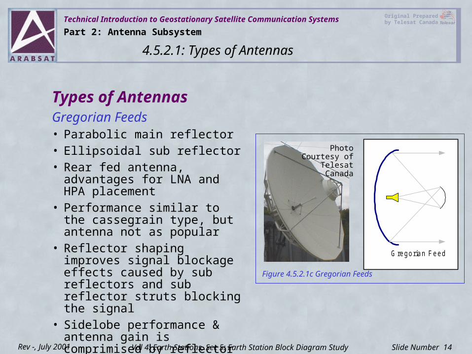
Types of AntennasGregorian Feeds• Parabolic main reflector• Ellipsoidal sub reflector • Rear fed antenna, advantages for
LNA and HPA placement• Performance similar to the
cassegrain type, but antenna not as popular
• Reflector shaping improves signal blockage effects caused by sub reflectors and sub reflector struts blocking the signal
• Sidelobe performance & antenna gain is comprimised by reflector shaping
G regorian Feed
Part 2: Antenna Subsystem
4.5.2.1: Types of Antennas
Vol 4: Earth Stations, Sec 5: Earth Station Block Diagram Study
Figure 4.5.2.1c Gregorian Feeds
Photo Courtesy of
Telesat Canada
Technical Introduction to Geostationary Satellite Communication Systems Original Prepared by Telesat Canada
Slide Number 15Rev -, July 2001
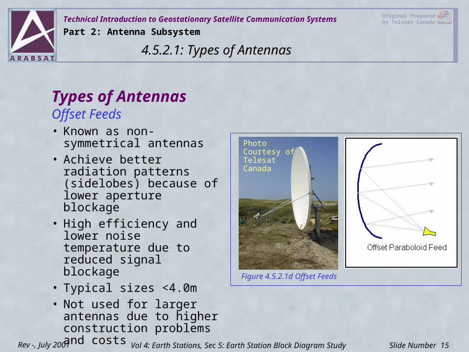
Types of AntennasOffset Feeds• Known as non-symmetrical
antennas• Achieve better radiation
patterns (sidelobes) because of lower aperture blockage
• High efficiency and lower noise temperature due to reduced signal blockage
• Typical sizes <4.0m• Not used for larger antennas
due to higher construction problems and costs
Part 2: Antenna Subsystem
4.5.2.1: Types of Antennas
Vol 4: Earth Stations, Sec 5: Earth Station Block Diagram Study
Figure 4.5.2.1d Offset Feeds
Photo Courtesy of Telesat Canada
Technical Introduction to Geostationary Satellite Communication Systems Original Prepared by Telesat Canada
Slide Number 16Rev -, July 2001
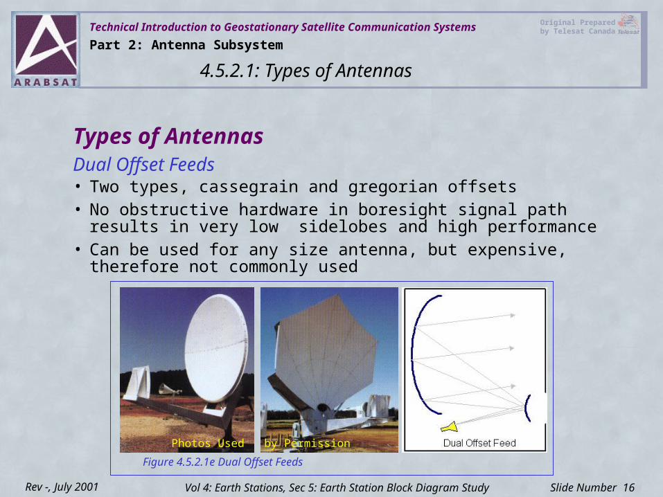
Types of AntennasDual Offset Feeds • Two types, cassegrain and gregorian offsets• No obstructive hardware in boresight signal path results in very low
sidelobes and high performance• Can be used for any size antenna, but expensive, therefore not
commonly used
Part 2: Antenna Subsystem
4.5.2.1: Types of Antennas
Vol 4: Earth Stations, Sec 5: Earth Station Block Diagram Study
Figure 4.5.2.1e Dual Offset Feeds
Photos Used by Permission
Technical Introduction to Geostationary Satellite Communication Systems Original Prepared by Telesat Canada
Slide Number 17Rev -, July 2001
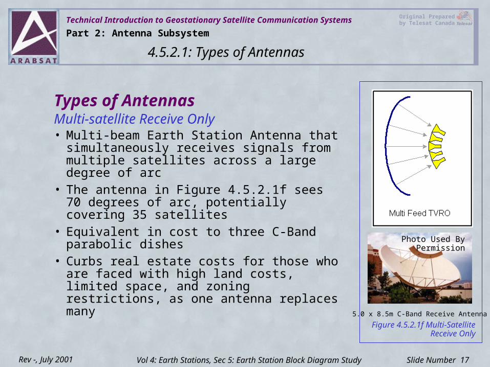
Types of AntennasMulti-satellite Receive Only• Multi-beam Earth Station Antenna that
simultaneously receives signals from multiple satellites across a large degree of arc
• The antenna in Figure 4.5.2.1f sees 70 degrees of arc, potentially covering 35 satellites
• Equivalent in cost to three C-Band parabolic dishes
• Curbs real estate costs for those who are faced with high land costs, limited space, and zoning restrictions, as one antenna replaces many
5.0 x 8.5m C-Band Receive Antenna
Part 2: Antenna Subsystem
4.5.2.1: Types of Antennas
Vol 4: Earth Stations, Sec 5: Earth Station Block Diagram Study
Figure 4.5.2.1f Multi-Satellite Receive Only
Photo Used By Permission
Technical Introduction to Geostationary Satellite Communication Systems Original Prepared by Telesat Canada
Slide Number 18Rev -, July 2001
Horn Main functions:• To illuminate main reflector• To separate transmit and receive bands• To separate and combine polarizations• To match impedance to that of free space• To provide error signals for some types of tracking systems
Feeds are open, flared waveguide sections. They can be rectangular or circular (conical).
Feedhorn design can drastically affect antenna performance.
Feed systems are composed primarily of a primary horn and a orthomode transducer (OMT).
Antenna feeds are designed for linear or circular polarization and must be adjusted to operate at the correct pole orientation.
Feeds
Part 2: Antenna Subsystem
4.5.2.2: Feeds
Vol 4: Earth Stations, Sec 5: Earth Station Block Diagram Study
Technical Introduction to Geostationary Satellite Communication Systems Original Prepared by Telesat Canada
Slide Number 19Rev -, July 2001
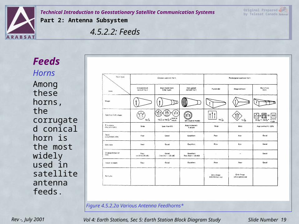
HornsAmong these horns, the corrugated conical horn is the most widely used in satellite antenna feeds.
Feeds
Part 2: Antenna Subsystem
4.5.2.2: Feeds
Vol 4: Earth Stations, Sec 5: Earth Station Block Diagram Study
Figure 4.5.2.2a Various Antenna Feedhorns*
Technical Introduction to Geostationary Satellite Communication Systems Original Prepared by Telesat Canada
Slide Number 20Rev -, July 2001
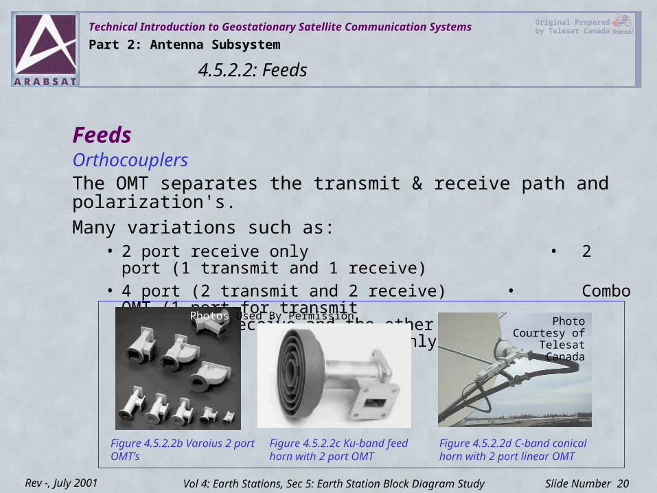
OrthocouplersThe OMT separates the transmit & receive path and polarization's.Many variations such as:
• 2 port receive only • 2 port (1 transmit and 1 receive)
• 4 port (2 transmit and 2 receive) • Combo OMT (1 port for transmit and receive and the other receive only)
Feeds
Figure 4.5.2.2d C-band conical horn with 2 port linear OMT
Figure 4.5.2.2c Ku-band feed horn with 2 port OMT
Figure 4.5.2.2b Varoius 2 port OMT’s
Part 2: Antenna Subsystem
4.5.2.2: Feeds
Vol 4: Earth Stations, Sec 5: Earth Station Block Diagram Study
Photo Courtesy of
Telesat Canada
Photos Used By Permission
Technical Introduction to Geostationary Satellite Communication Systems Original Prepared by Telesat Canada
Slide Number 21Rev -, July 2001
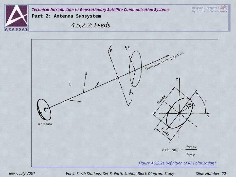
Polarization, Linear and CircularThe polarization of an RF wave radiated or received by an antenna is defined by the orientation of the electric vector E of the wave (Figure 4.5.2.2e).
This vector, which is perpendicular to the direction of propagation, can vary in direction & intensity during one RF period.
Feeds
While travelling one wavelength during one period, the E vector not only oscillates in intensity but can also rotate.
In the most general case, the projection of the tip of the E vector on a plane P perpendicular to the direction of propagation describes an ellipse during one period. This is called elliptical polarization.
Part 2: Antenna Subsystem
4.5.2.2: Feeds
Vol 4: Earth Stations, Sec 5: Earth Station Block Diagram Study
Technical Introduction to Geostationary Satellite Communication Systems Original Prepared by Telesat Canada
Slide Number 22Rev -, July 2001
Figure 4.5.2.2e Definition of RF Polarization*
Part 2: Antenna Subsystem
4.5.2.2: Feeds
Vol 4: Earth Stations, Sec 5: Earth Station Block Diagram Study
Technical Introduction to Geostationary Satellite Communication Systems Original Prepared by Telesat Canada
Slide Number 23Rev -, July 2001
FeedsPolarization, Linear and CircularElliptical polarization is characterized by 3 parameters:
• Rotation sense, as seen from the antenna and looking in the direction of propagation: right hand (RH - clockwise) or left hand (LH - counter-clockwise)
• Axial ratio (AR) of the ellipse (voltage axial ratio) • Inclination angle (T) of the ellipse
Most practical antennas radiate either in linear polarization (LP) or in circular polarization (CP) which are the most common particular cases of elliptical polarization.Linear polarization is obtained when the axial ratio is infinite, i.e. the ellipse is completely flat.
Circular polarization is obtained when Axial Ratio, AR=1.
Part 2: Antenna Subsystem
4.5.2.2: Feeds
Vol 4: Earth Stations, Sec 5: Earth Station Block Diagram Study
Technical Introduction to Geostationary Satellite Communication Systems Original Prepared by Telesat Canada
Slide Number 24Rev -, July 2001
FeedsOrthogonal PolarizationTwo waves are in orthogonal polarization if their electric fields describe identical ellipses in opposite directions.
Examples Two orthogonal circular polarizations described as right hand circular and left hand circular.Two orthogonal linear polarizations described as horizontal & vertical (relative to a local reference).
Part 2: Antenna Subsystem
4.5.2.2: Feeds
Vol 4: Earth Stations, Sec 5: Earth Station Block Diagram Study
Technical Introduction to Geostationary Satellite Communication Systems Original Prepared by Telesat Canada
Slide Number 25Rev -, July 2001
FeedsOrthogonal PolarizationExamples An antenna designed to transmit or receive a wave of a given polarization can neither transmit nor receive in the orthogonal polarization.
This property enables two simultaneous links to be established at the same frequency between the same two locations. This is called frequency reuse by orthogonal polarization.
Hence we have LHCP & RHCP or in linear polarization, vertical & horizontal.
Part 2: Antenna Subsystem
4.5.2.2: Feeds
Vol 4: Earth Stations, Sec 5: Earth Station Block Diagram Study
Technical Introduction to Geostationary Satellite Communication Systems Original Prepared by Telesat Canada
Slide Number 26Rev -, July 2001
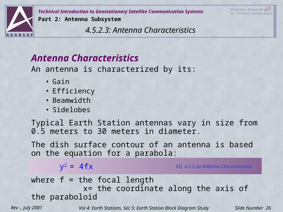
Antenna CharacteristicsAn antenna is characterized by its:
• Gain • Efficiency• Beamwidth• Sidelobes
Typical Earth Station antennas vary in size from 0.5 meters to 30 meters in diameter.
The dish surface contour of an antenna is based on the equation for a parabola:
y2 = 4fx
where f = the focal length x= the coordinate along the axis of the paraboloid
Part 2: Antenna Subsystem
4.5.2.3: Antenna Characteristics
Vol 4: Earth Stations, Sec 5: Earth Station Block Diagram Study
EQ. 4.5.2.3a Antenna Characteristics
Technical Introduction to Geostationary Satellite Communication Systems Original Prepared by Telesat Canada
Slide Number 27Rev -, July 2001
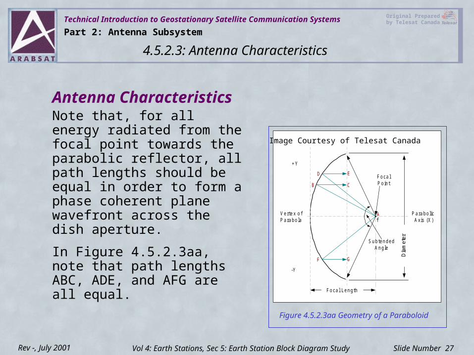
Antenna CharacteristicsNote that, for all energy radiated from the focal point towards the parabolic reflector, all path lengths should be equal in order to form a phase coherent plane wavefront across the dish aperture.
In Figure 4.5.2.3aa, note that path lengths ABC, ADE, and AFG are all equal.
Part 2: Antenna Subsystem
4.5.2.3: Antenna Characteristics
Vol 4: Earth Stations, Sec 5: Earth Station Block Diagram Study
Dia
met
er
Parabo lic Axis (X)
V ertex o fP arabola
+Y
-Y
Foca lP oint
f
Foca l Length
A
B C
D E
F G
S ubtendedAngle
Figure 4.5.2.3aa Geometry of a Paraboloid
Image Courtesy of Telesat Canada
Technical Introduction to Geostationary Satellite Communication Systems Original Prepared by Telesat Canada
Slide Number 28Rev -, July 2001
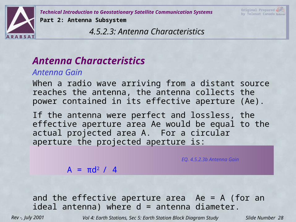
Antenna CharacteristicsAntenna GainWhen a radio wave arriving from a distant source reaches the antenna, the antenna collects the power contained in its effective aperture (Ae).
If the antenna were perfect and lossless, the effective aperture area Ae would be equal to the actual projected area A. For a circular aperture the projected aperture is:
A = πd2 / 4
and the effective aperture area Ae = A (for an ideal antenna) where d = antenna diameter.
Part 2: Antenna Subsystem
4.5.2.3: Antenna Characteristics
Vol 4: Earth Stations, Sec 5: Earth Station Block Diagram Study
EQ. 4.5.2.3b Antenna Gain
Technical Introduction to Geostationary Satellite Communication Systems Original Prepared by Telesat Canada
Slide Number 29Rev -, July 2001
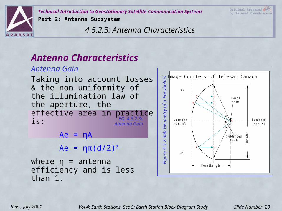
Antenna CharacteristicsAntenna GainTaking into account losses & the non-uniformity of the illumination law of the aperture, the effective area in practice is:
Ae = ηA
Ae = ηπ(d/2)2
where η = antenna efficiency and is less than 1.
Dia
met
er
Pa rabo lic Axis (X)
V ertex o fP arabola
+Y
-Y
FocalP o in t
f
Foca l Length
A
B C
D E
F G
SubtendedA ngle
Figu
re 4
.5.2
.3ab
Geo
met
ry o
f a P
arab
oloi
d
Part 2: Antenna Subsystem
4.5.2.3: Antenna Characteristics
Vol 4: Earth Stations, Sec 5: Earth Station Block Diagram Study
Image Courtesy of Telesat Canada
EQ. 4.5.2.3c Antenna Gain
Technical Introduction to Geostationary Satellite Communication Systems Original Prepared by Telesat Canada
Slide Number 30Rev -, July 2001
Antenna CharacteristicsEfficiencyEfficiency is an important factor in antenna design. Special techniques such as reflector shaping are used to optimize the efficiency of an Earth Station antenna.
Antenna aperture efficiencies between 55 and 75 percent are typically obtainable depending on type and design.
Efficiency is affected by:• Subreflector and supporting hardware
• Main reflector RMS surface deviation
• Illumination efficiency, which accounts for the non uniformity of the illumination, phase distribution across the antenna surface and power radiated in the sidelobes
Part 2: Antenna Subsystem
4.5.2.3: Antenna Characteristics
Vol 4: Earth Stations, Sec 5: Earth Station Block Diagram Study
Technical Introduction to Geostationary Satellite Communication Systems Original Prepared by Telesat Canada
Slide Number 31Rev -, July 2001
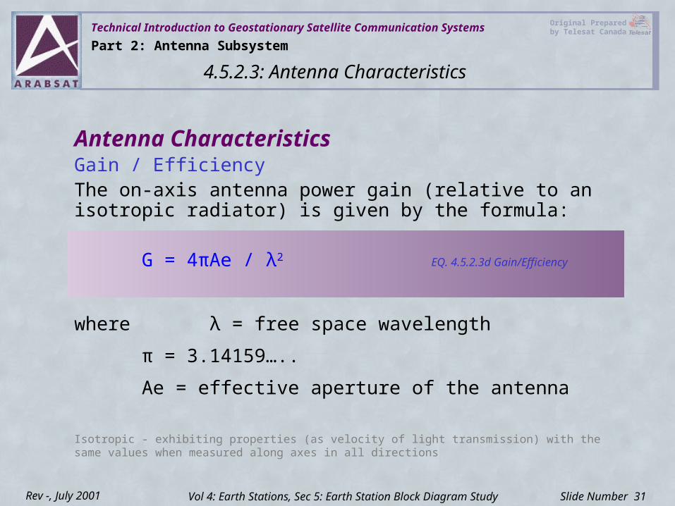
Antenna CharacteristicsGain / EfficiencyThe on-axis antenna power gain (relative to an isotropic radiator) is given by the formula:
G = 4πAe / λ2
where λ = free space wavelength
π = 3.14159…..
Ae = effective aperture of the antenna
Isotropic - exhibiting properties (as velocity of light transmission) with the same values when measured along axes in all directions
Part 2: Antenna Subsystem
4.5.2.3: Antenna Characteristics
Vol 4: Earth Stations, Sec 5: Earth Station Block Diagram Study
EQ. 4.5.2.3d Gain/Efficiency
Technical Introduction to Geostationary Satellite Communication Systems Original Prepared by Telesat Canada
Slide Number 32Rev -, July 2001
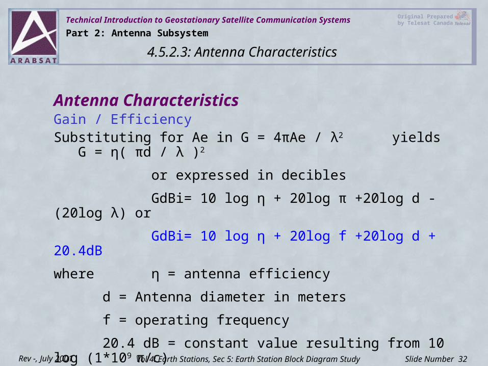
Antenna CharacteristicsGain / EfficiencySubstituting for Ae in G = 4πAe / λ2 yields G = η( πd / λ )2
or expressed in decibles
GdBi= 10 log η + 20log π +20log d - (20log λ) or
GdBi= 10 log η + 20log f +20log d + 20.4dB
where η = antenna efficiency
d = Antenna diameter in meters
f = operating frequency
20.4 dB = constant value resulting from 10 log (1*109 π/c)
Part 2: Antenna Subsystem
4.5.2.3: Antenna Characteristics
Vol 4: Earth Stations, Sec 5: Earth Station Block Diagram Study
Technical Introduction to Geostationary Satellite Communication Systems Original Prepared by Telesat Canada
Slide Number 33Rev -, July 2001
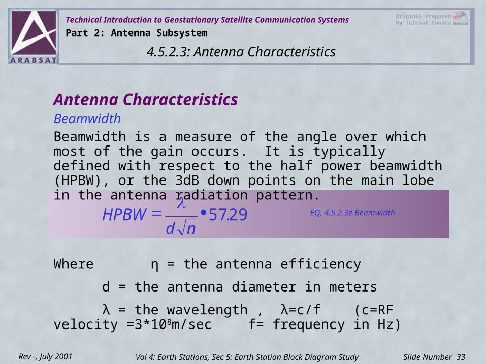
Antenna CharacteristicsBeamwidthBeamwidth is a measure of the angle over which most of the gain occurs. It is typically defined with respect to the half power beamwidth (HPBW), or the 3dB down points on the main lobe in the antenna radiation pattern.
Where η = the antenna efficiency
d = the antenna diameter in meters
λ = the wavelength , λ=c/f (c=RF velocity =3*108m/sec f= frequency in Hz)
Part 2: Antenna Subsystem
4.5.2.3: Antenna Characteristics
Vol 4: Earth Stations, Sec 5: Earth Station Block Diagram Study
29.57nd
HPBW
EQ. 4.5.2.3e Beamwidth

Technical Introduction to Geostationary Satellite Communication Systems Original Prepared by Telesat Canada
Slide Number 34Rev -, July 2001
Antenna CharacteristicsBeamwidthExample An Intelsat Standard “A” Earth Station with an antenna size of 16 meters and an efficiency of 70 percent would thus have a beamwidth of 0.214 degree at 6GHz.
η = .70
d = 16
λ = c/f = (3*108m/sec)/6,000,000,000 = .05
Part 2: Antenna Subsystem
4.5.2.3: Antenna Characteristics
Vol 4: Earth Stations, Sec 5: Earth Station Block Diagram Study
21398.
29.5770.16
05.
HPBW
HPBW
or 0.214
Technical Introduction to Geostationary Satellite Communication Systems Original Prepared by Telesat Canada
Slide Number 35Rev -, July 2001
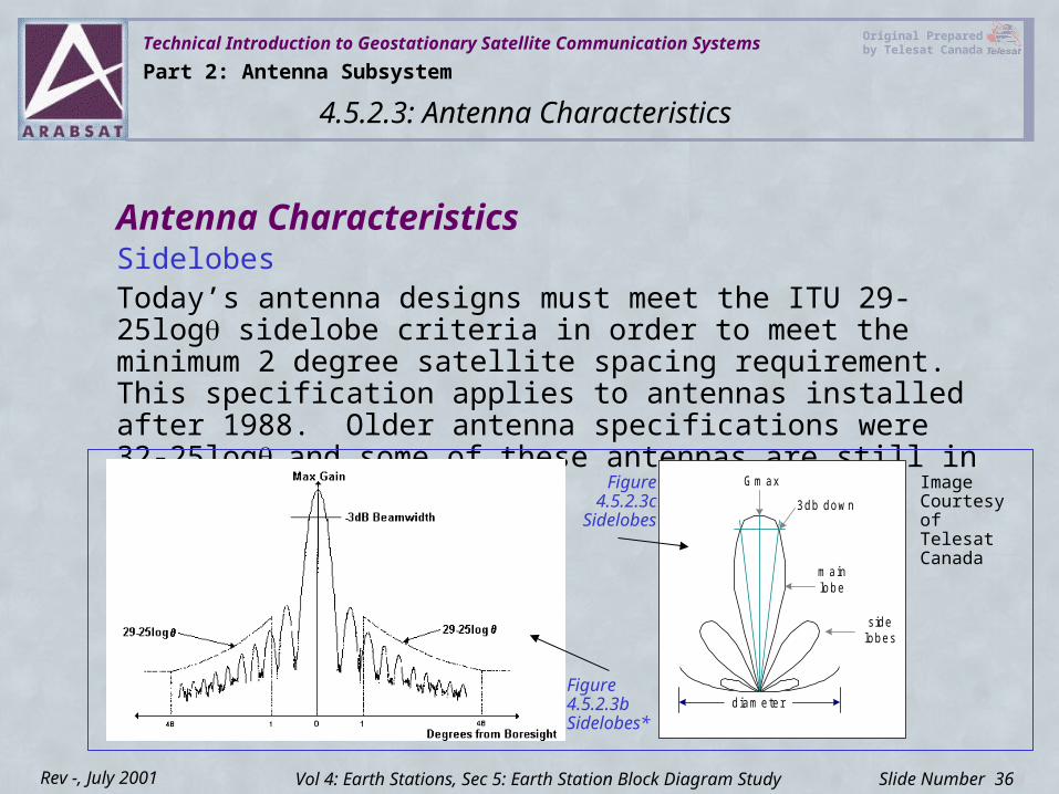
Antenna CharacteristicsSidelobesMost of the power radiated by an antenna is contained in the main lobe. However, a certain amount of residual power is radiated into the sidelobes.
Sidelobes are an intrinsic property of antenna radiation and cannot be completely eliminated. They can, however, be reduced by careful design.
The side lobe characteristic of Earth Station antennas is one of the main factors in determining the minimum spacing requirements between satellites and therefore the orbit/spectrum utilization efficiency.
Other factors effecting sidelobe characteristics are antenna diameter, operating frequency, and aperture efficiency.
Part 2: Antenna Subsystem
4.5.2.3: Antenna Characteristics
Vol 4: Earth Stations, Sec 5: Earth Station Block Diagram Study
Technical Introduction to Geostationary Satellite Communication Systems Original Prepared by Telesat Canada
Slide Number 36Rev -, July 2001
Antenna CharacteristicsSidelobesToday’s antenna designs must meet the ITU 29-25log sidelobe criteria in order to meet the minimum 2 degree satellite spacing requirement. This specification applies to antennas installed after 1988. Older antenna specifications were 32-25logand some of these antennas are still in service.
G m ax
3db down
m ainlobe
sidelobes
d iam eter
Part 2: Antenna Subsystem
4.5.2.3: Antenna Characteristics
Vol 4: Earth Stations, Sec 5: Earth Station Block Diagram Study
Figure 4.5.2.3b Sidelobes*
Figure 4.5.2.3c
Sidelobes
Image Courtesy of Telesat Canada
Technical Introduction to Geostationary Satellite Communication Systems Original Prepared by Telesat Canada
Slide Number 37Rev -, July 2001
Antenna StructuresMount and FoundationEnvironmental Conditions for Design:There are differences in design standards and Codes used in various countries however the end result of the design process is often very similar.
Wind, Ice, Other Wind is the most significant design parameter and typically governs the structural design for survival strength and also for operational stiffness.
In areas where ice loading occurs, load combinations such as ice with half wind load, must be considered.
Part 2: Antenna Subsystem
4.5.2.4: Antenna Structures
Vol 4: Earth Stations, Sec 5: Earth Station Block Diagram Study
Technical Introduction to Geostationary Satellite Communication Systems Original Prepared by Telesat Canada
Slide Number 38Rev -, July 2001
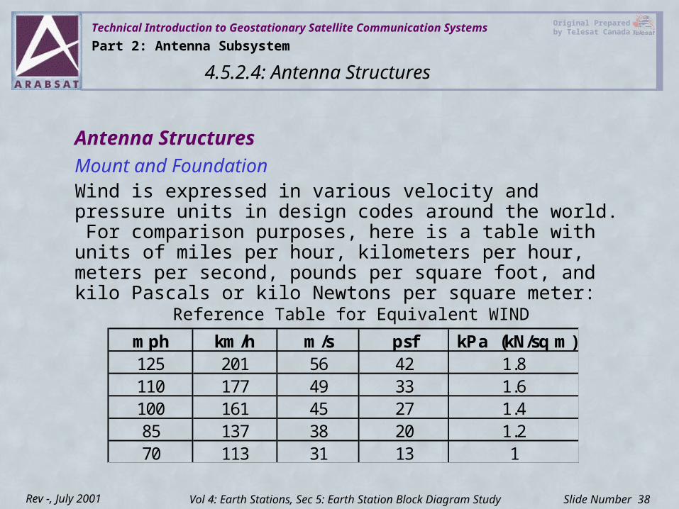
Mount and FoundationWind is expressed in various velocity and pressure units in design codes around the world. For comparison purposes, here is a table with units of miles per hour, kilometers per hour, meters per second, pounds per square foot, and kilo Pascals or kilo Newtons per square meter:
Reference Table for Equivalent WINDmph km/h m/s psf kPa (kN/sq m)125 201 56 42 1.8110 177 49 33 1.6100 161 45 27 1.485 137 38 20 1.270 113 31 13 1
Antenna Structures
Part 2: Antenna Subsystem
4.5.2.4: Antenna Structures
Vol 4: Earth Stations, Sec 5: Earth Station Block Diagram Study
Technical Introduction to Geostationary Satellite Communication Systems Original Prepared by Telesat Canada
Slide Number 39Rev -, July 2001
Antenna StructuresMount and FoundationWind Overview of Design Methods used in Canada and the United States:
The hourly average pressure for a 10 year return period Wind is used in Canada for antennas with area not more than 5 square meters.
The hourly average pressure for a 30 year return period Wind is used in Canada for larger antennas and typical building construction.
The velocity of the “fastest mile” 50 year return period Wind is used in US design.
Part 2: Antenna Subsystem
4.5.2.4: Antenna Structures
Vol 4: Earth Stations, Sec 5: Earth Station Block Diagram Study
Technical Introduction to Geostationary Satellite Communication Systems Original Prepared by Telesat Canada
Slide Number 40Rev -, July 2001
Mount and FoundationWind Understanding the Various Design Approaches:In Canada, Wind Design is derived from the maximum hourly average pressure for an appropriate return period wind, which is then modified with a gust factor and various other site-specific factors to obtain the design loads.
In the United States, Wind Design is determined from the fastest mile of wind which is the highest sustained average wind speed based on the time required for mile-long sample of air to pass a fixed point. This speed of wind is converted to pressure and a gust factor and other factors are then applied to obtain design loads.
Antenna Structures
Part 2: Antenna Subsystem
4.5.2.4: Antenna Structures
Vol 4: Earth Stations, Sec 5: Earth Station Block Diagram Study

Technical Introduction to Geostationary Satellite Communication Systems Original Prepared by Telesat Canada
Slide Number 41Rev -, July 2001
Mount and FoundationReturn Period for Design Wind: The probability of wind occurring in any year can be derived directly from the Return Period. A 30 year wind has a 1 in 30 chance of occurring in any year, which is a 3% probability. A 10 year wind has a 10% chance of occurring in any year.
10 year Wind - Used in Canada with gust factor of 2.5 on pressure for antennas of < 5 square meter area.
30 year Wind - Used in Canada with gust factor of 2.0 on pressure for antennas of > 5 square meter area.
Antenna Structures
Part 2: Antenna Subsystem
4.5.2.4: Antenna Structures
Vol 4: Earth Stations, Sec 5: Earth Station Block Diagram Study
Technical Introduction to Geostationary Satellite Communication Systems Original Prepared by Telesat Canada
Slide Number 42Rev -, July 2001
Mount and FoundationReturn Period for Design Wind: 50 year Wind - Used in U.S. These design codes use a smaller effective gust factor since the measuring period of the “fastest mile” is a much shorter time period. For high wind areas, the fastest mile could be perhaps only 30 seconds duration. Therefore the gust factor associated with a 30 second wind is smaller compared to the gust factor for an hourly average reference.
100 year Wind - Used in Canada and elsewhere for critical and post disaster services. Gust factors same as above.
Antenna Structures
Part 2: Antenna Subsystem
4.5.2.4: Antenna Structures
Vol 4: Earth Stations, Sec 5: Earth Station Block Diagram Study
Technical Introduction to Geostationary Satellite Communication Systems Original Prepared by Telesat Canada
Slide Number 43Rev -, July 2001
Mount and FoundationGust Factor: Since antennas are all relatively small structures, they respond to gusts. Gusts are wind speeds that are normally defined as having 5 second duration. Therefore, the gust wind must be used in structural adequacy calculations.
If the type of service carried by the antenna is affected by even momentary outages, then elastic deflections for the peak gust wind must also be used for design purposes.
Antenna Structures
Part 2: Antenna Subsystem
4.5.2.4: Antenna Structures
Vol 4: Earth Stations, Sec 5: Earth Station Block Diagram Study
Technical Introduction to Geostationary Satellite Communication Systems Original Prepared by Telesat Canada
Slide Number 44Rev -, July 2001
Mount and FoundationGust Factor: To determine the force acting on an object (antenna), the design wind pressure is multiplied by the (frontal) full-face area of the antenna and the shape factor.
The shape factor is different for all directions and in published data this normally includes an adjustment for the effective antenna area which is in the wind for each of the wind directions considered.
The typical maximum shape factor for a parabolic antenna is approximately 1.5.
Antenna Structures
Part 2: Antenna Subsystem
4.5.2.4: Antenna Structures
Vol 4: Earth Stations, Sec 5: Earth Station Block Diagram Study
Technical Introduction to Geostationary Satellite Communication Systems Original Prepared by Telesat Canada
Slide Number 45Rev -, July 2001
Mount and FoundationHeight Factor: Wind velocity increases with height above ground (up to approximately 500 meters).
Wind velocity near the ground surface is also influenced by the roughness factor of the surface. Near the ground, wind speed is higher over flat land or open water than it is in an urban or forested location or where there are surface irregularities.
Antenna Structures
Part 2: Antenna Subsystem
4.5.2.4: Antenna Structures
Vol 4: Earth Stations, Sec 5: Earth Station Block Diagram Study
Technical Introduction to Geostationary Satellite Communication Systems Original Prepared by Telesat Canada
Slide Number 46Rev -, July 2001
Mount and FoundationHeight Factor: Height factors (applied to wind pressure for design purposes) are:
0.9 for up to 6m height
1.0 for 10m height
1.15 for 20m height
1.25 for 30m height
Design winds are derived from observations of wind recorded at a standard height of 10m in open areas (typically airport locations). The height factors are applied to these values to determine wind at the desired elevation.
Antenna Structures
Part 2: Antenna Subsystem
4.5.2.4: Antenna Structures
Vol 4: Earth Stations, Sec 5: Earth Station Block Diagram Study
Technical Introduction to Geostationary Satellite Communication Systems Original Prepared by Telesat Canada
Slide Number 47Rev -, July 2001
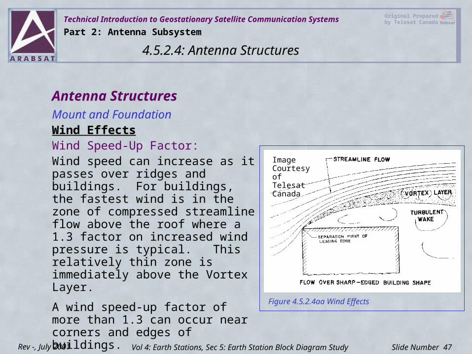
Mount and FoundationWind Effects Wind Speed-Up Factor:Wind speed can increase as it passes over ridges and buildings. For buildings, the fastest wind is in the zone of compressed streamline flow above the roof where a 1.3 factor on increased wind pressure is typical. This relatively thin zone is immediately above the Vortex Layer.
A wind speed-up factor of more than 1.3 can occur near corners and edges of buildings.
Antenna Structures
Part 2: Antenna Subsystem
4.5.2.4: Antenna Structures
Vol 4: Earth Stations, Sec 5: Earth Station Block Diagram Study
Figure 4.5.2.4aa Wind Effects
Image Courtesy of Telesat Canada
Technical Introduction to Geostationary Satellite Communication Systems Original Prepared by Telesat Canada
Slide Number 48Rev -, July 2001
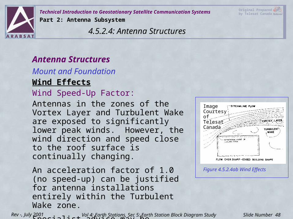
Antenna StructuresMount and FoundationWind Effects Wind Speed-Up Factor:Antennas in the zones of the Vortex Layer and Turbulent Wake are exposed to significantly lower peak winds. However, the wind direction and speed close to the roof surface is continually changing.
An acceleration factor of 1.0 (no speed-up) can be justified for antenna installations entirely within the Turbulent Wake zone.
Specialist advice may be required to make specific design recommendations for roof mounted antennas.
Part 2: Antenna Subsystem
4.5.2.4: Antenna Structures
Vol 4: Earth Stations, Sec 5: Earth Station Block Diagram Study
Figure 4.5.2.4ab Wind Effects
Image Courtesy of Telesat Canada
Technical Introduction to Geostationary Satellite Communication Systems Original Prepared by Telesat Canada
Slide Number 49Rev -, July 2001
Mount and FoundationIce: The build-up of ice on structures is a function of the amount, nature, and angle of rain occurring at just-freezing temperatures. Ice can also accumulate from fog. At temperatures below -10º C, is buildup is unlikely.
Freezing Rain (glaze ice): In conditions of freezing rain and high winds, it is possible to have significantly thicker ice build-up on vertical surfaces than the actual depth of rain water. This ice is “clear” and has a density of 90% that of water.
Antenna Structures
Part 2: Antenna Subsystem
4.5.2.4: Antenna Structures
Vol 4: Earth Stations, Sec 5: Earth Station Block Diagram Study
Technical Introduction to Geostationary Satellite Communication Systems Original Prepared by Telesat Canada
Slide Number 50Rev -, July 2001
Mount and FoundationIn-Cloud Icing (rime ice):In-cloud icing normally occurs at higher elevations in coastal areas when moist clouds (fog) remain for a period of time with the structures at a temperature below freezing. Several hundred meters of elevation is often the difference between no icing and a severe problem. Rime ice is white and opaque with a density that varies between 30% and 70% that of water and a texture from soft to hard depending on conditions during forming. The total thickness of rime ice depends more on the time of exposure to conditions which promote that growth.
Ice load can be multiples of the weight of the antenna structures and are a serious consideration in affected areas.
Antenna Structures
Part 2: Antenna Subsystem
4.5.2.4: Antenna Structures
Vol 4: Earth Stations, Sec 5: Earth Station Block Diagram Study
Technical Introduction to Geostationary Satellite Communication Systems Original Prepared by Telesat Canada
Slide Number 51Rev -, July 2001
Mount and FoundationOther Conditions: Seismic Seismic design generally does not govern any of the structural decisions made when selecting antennas and mounts.
For satellite communication antennas (parabolic shapes with large surface area compared to weight) the design forces due to wind are much more than the lateral, seismic loads due to earthquake shaking.
For example, seismic loading of up to 20% of the weight of the structure taken as a lateral force is much less than typical wind loads.The seismic performance of a communication facility is much more dependent on supporting the indoor equipment to prevent movement and the survivability of cabling and services (especially with underground conduits).
Antenna Structures
Part 2: Antenna Subsystem
4.5.2.4: Antenna Structures
Vol 4: Earth Stations, Sec 5: Earth Station Block Diagram Study
Technical Introduction to Geostationary Satellite Communication Systems Original Prepared by Telesat Canada
Slide Number 52Rev -, July 2001
Mount and FoundationDesign Wind for “Survival”The word “survival” is often used to describe the design conditions, such as the maximum design wind speed.
However, design codes use these conditions to safely engineer the structures to withstand the loads without damage, yielding or deformation of parts. Therefore, each structure has a margin of failure beyond the design loads.
For steel design in Canada and the U. S., there is a minimum factor to theoretical failure of 1.67. This is applicable to tension member failure. Other and more critical modes of failure which can result in immediate collapse of a structure have higher margins to failure. For example, compression buckling of slender members is 1.92 and bolt connections have a factor of 2.5.
Antenna Structures
Part 2: Antenna Subsystem
4.5.2.4: Antenna Structures
Vol 4: Earth Stations, Sec 5: Earth Station Block Diagram Study
Technical Introduction to Geostationary Satellite Communication Systems Original Prepared by Telesat Canada
Slide Number 53Rev -, July 2001
Mount and FoundationDesign Wind for “Survival”Other materials, such as aluminum, fiberglass, or concrete, are intended to have an equivalent level of confidence and have “safety factors” adjusted accordingly to suit the material and fabrication methods.
A 100 year wind has a pressure that is typically no more than 25% greater than a 30 year wind. When you consider that the structure has a minimum 1.67 factor, there are few conditions which should ever result in antenna collapse.
Antenna Structures
Part 2: Antenna Subsystem
4.5.2.4: Antenna Structures
Vol 4: Earth Stations, Sec 5: Earth Station Block Diagram Study
Technical Introduction to Geostationary Satellite Communication Systems Original Prepared by Telesat Canada
Slide Number 54Rev -, July 2001
Mount and FoundationDesign Wind for “Operational” ConditionsThe Operational limit of an antenna is the wind speed which creates a signal loss of defined level (dB) as a result of elastic deflections.
(Motorized antennas may also specify a maximum wind to operate the motors.)
Signal loss is due primarily to the off-axis movement of the antenna rather than antenna distortion, feed movement or other condition. All deflections can be considered as elastic and when the wind force is removed, original signal strength is regained.
Antenna Structures
Part 2: Antenna Subsystem
4.5.2.4: Antenna Structures
Vol 4: Earth Stations, Sec 5: Earth Station Block Diagram Study
Technical Introduction to Geostationary Satellite Communication Systems Original Prepared by Telesat Canada
Slide Number 55Rev -, July 2001
Mount and FoundationDesign Wind for “Operational” ConditionsThe antenna pattern will provide the angle of off-axis movement which will result in the signal loss being considered. Understand-ing the manufacturer’s definition of “operational” is essential to confirm that the performance of the installed antenna system will be as expected.
The operational wind limit is a wind velocity. However:• It may represent an averaged effect for all directions• It may represent an average for all possible elevation angles of
the antenna (up to 90 degrees in some cases) • It may represent an average of the full adjustment range of the
antenna (full left, center, full right), and sometimes a mount is not as stiff in all configurations
Antenna Structures
Part 2: Antenna Subsystem
4.5.2.4: Antenna Structures
Vol 4: Earth Stations, Sec 5: Earth Station Block Diagram Study
Technical Introduction to Geostationary Satellite Communication Systems Original Prepared by Telesat Canada
Slide Number 56Rev -, July 2001
Mount and FoundationDesign Wind for “Operational” Conditions
• It may be stated as a gust wind, but in reality include averaging to minimize the effects of gusts.
• Normally there is no allowance for foundation movement in operational deflection calculations. This is satisfactory for ground mounts, but it is not realistic for roof installations that must include deflections of foundation beams etc. If 15% of the allowable movement is allocated to the foundation, the effective operational wind limit of the antenna has been reduced by approximately 7%.
Antenna Structures
Part 2: Antenna Subsystem
4.5.2.4: Antenna Structures
Vol 4: Earth Stations, Sec 5: Earth Station Block Diagram Study
Technical Introduction to Geostationary Satellite Communication Systems Original Prepared by Telesat Canada
Slide Number 57Rev -, July 2001
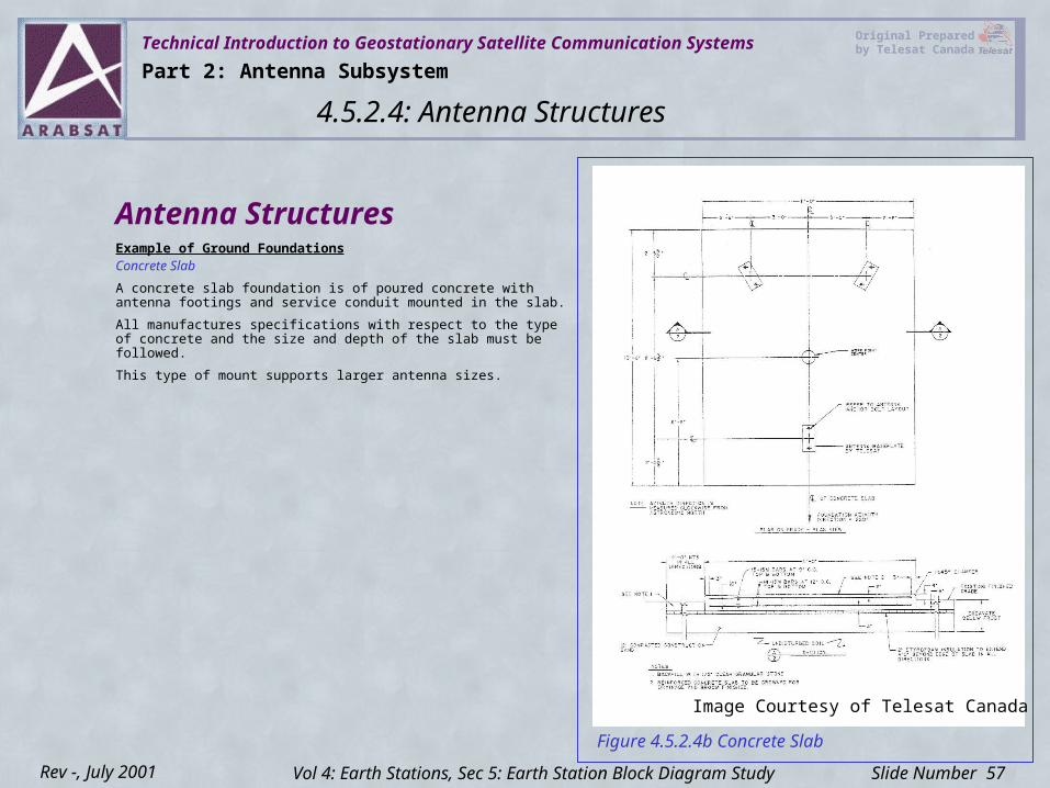
Example of Ground FoundationsConcrete Slab
A concrete slab foundation is of poured concrete with antenna footings and service conduit mounted in the slab.
All manufactures specifications with respect to the type of concrete and the size and depth of the slab must be followed.
This type of mount supports larger antenna sizes.
Antenna Structures
Part 2: Antenna Subsystem
4.5.2.4: Antenna Structures
Vol 4: Earth Stations, Sec 5: Earth Station Block Diagram Study
Figure 4.5.2.4b Concrete Slab
Image Courtesy of Telesat Canada
Technical Introduction to Geostationary Satellite Communication Systems Original Prepared by Telesat Canada
Slide Number 58Rev -, July 2001
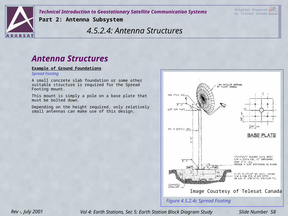
Example of Ground FoundationsSpread Footing
A small concrete slab foundation or some other suitable structure is required for the Spread Footing mount.
This mount is simply a pole on a base plate that must be bolted down.
Depending on the height required, only relatively small antennas can make use of this design.
Antenna Structures
Part 2: Antenna Subsystem
4.5.2.4: Antenna Structures
Vol 4: Earth Stations, Sec 5: Earth Station Block Diagram Study
Figure 4.5.2.4c Spread Footing
Image Courtesy of Telesat Canada
Technical Introduction to Geostationary Satellite Communication Systems Original Prepared by Telesat Canada
Slide Number 59Rev -, July 2001
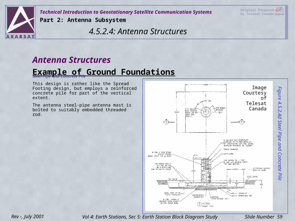
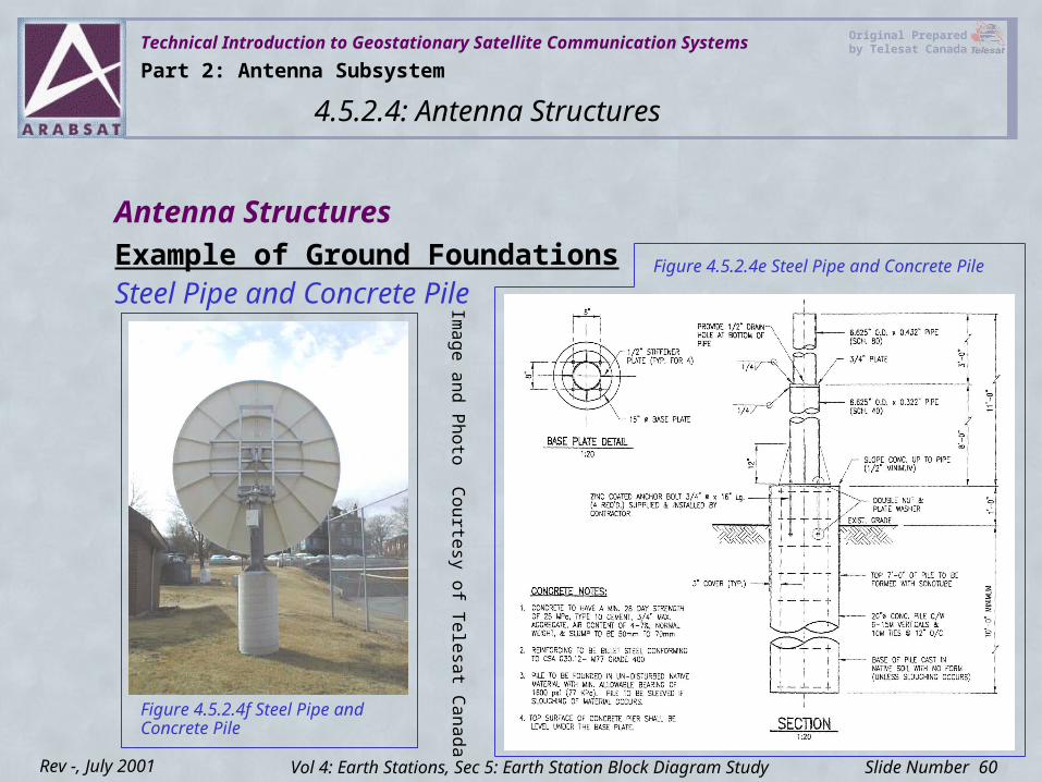
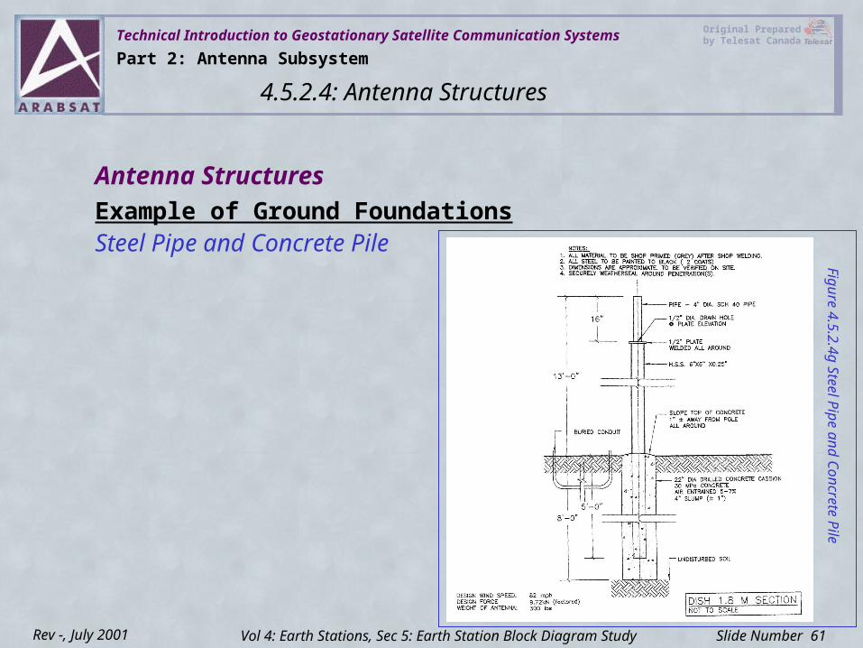
Steel Pipe and Concrete Pile
This design is rather like the Spread Footing design, but employs a reinforced concrete pile for part of the vertical extent.
The antenna steel-pipe antenna mast is bolted to suitably embedded threaded rod.
Antenna Structures
Part 2: Antenna Subsystem
4.5.2.4: Antenna Structures
Vol 4: Earth Stations, Sec 5: Earth Station Block Diagram Study
Figure 4.5.2.4d Steel P
ipe and Concrete
PileImage
Courtesy of Telesat
Canada
Example of Ground Foundations
Technical Introduction to Geostationary Satellite Communication Systems Original Prepared by Telesat Canada
Slide Number 60Rev -, July 2001
Example of Ground FoundationsSteel Pipe and Concrete Pile
Antenna Structures
Part 2: Antenna Subsystem
4.5.2.4: Antenna Structures
Vol 4: Earth Stations, Sec 5: Earth Station Block Diagram Study
Figure 4.5.2.4e Steel Pipe and Concrete Pile
Figure 4.5.2.4f Steel Pipe and Concrete Pile
Image and Photo Courtesy of Telesat Canada
Technical Introduction to Geostationary Satellite Communication Systems Original Prepared by Telesat Canada
Slide Number 61Rev -, July 2001
Example of Ground FoundationsSteel Pipe and Concrete Pile
Antenna Structures
Part 2: Antenna Subsystem
4.5.2.4: Antenna Structures
Vol 4: Earth Stations, Sec 5: Earth Station Block Diagram Study
Figure 4.5.2.4g Steel P
ipe and Concrete P
ile
Technical Introduction to Geostationary Satellite Communication Systems Original Prepared by Telesat Canada
Slide Number 62Rev -, July 2001
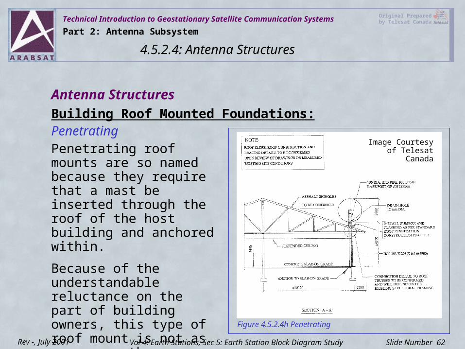
Building Roof Mounted Foundations:Penetrating
Antenna Structures
Part 2: Antenna Subsystem
4.5.2.4: Antenna Structures
Vol 4: Earth Stations, Sec 5: Earth Station Block Diagram Study
Figure 4.5.2.4h Penetrating
Image Courtesy of Telesat CanadaPenetrating roof mounts are
so named because they require that a mast be inserted through the roof of the host building and anchored within.
Because of the understandable reluctance on the part of building owners, this type of roof mount is not as common as the non-penetrating type.
Technical Introduction to Geostationary Satellite Communication Systems Original Prepared by Telesat Canada
Slide Number 63Rev -, July 2001
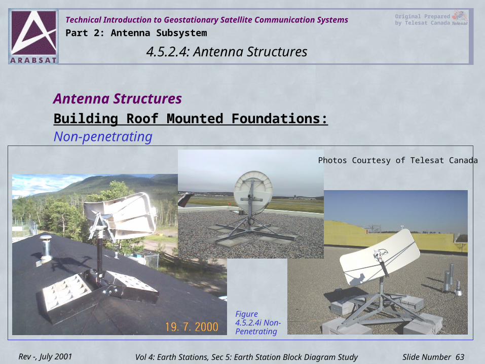
Building Roof Mounted Foundations:Non-penetrating
Antenna Structures
Part 2: Antenna Subsystem
4.5.2.4: Antenna Structures
Vol 4: Earth Stations, Sec 5: Earth Station Block Diagram Study
Figure 4.5.2.4i Non-Penetrating
Photos Courtesy of Telesat Canada
Technical Introduction to Geostationary Satellite Communication Systems Original Prepared by Telesat Canada
Slide Number 64Rev -, July 2001
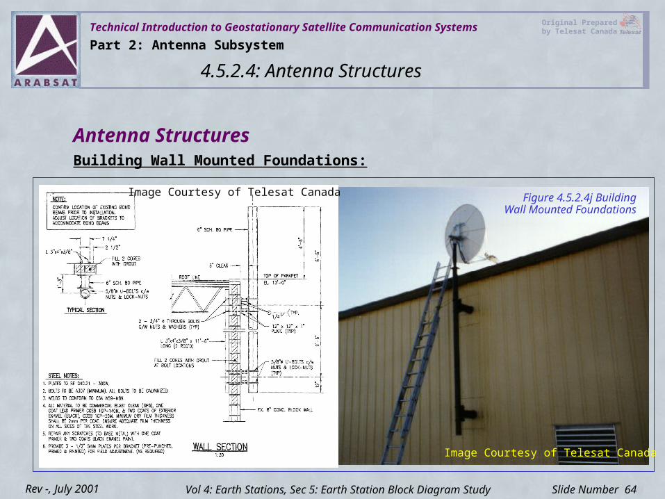
Building Wall Mounted Foundations:Antenna Structures
Part 2: Antenna Subsystem
4.5.2.4: Antenna Structures
Vol 4: Earth Stations, Sec 5: Earth Station Block Diagram Study
Figure 4.5.2.4j Building Wall Mounted Foundations
Image Courtesy of Telesat Canada
Image Courtesy of Telesat Canada
Technical Introduction to Geostationary Satellite Communication Systems Original Prepared by Telesat Canada
Slide Number 65Rev -, July 2001
Tracking SystemsIntroductionAlthough satellites are in geostationary orbits, they are constantly subjected to forces such as the gravitational attraction of the sun and moon, the radiation force of the sun’s light, and the sun’s own gravitational field.
These forces affect the position of the satellite and cause the satellite to drift from its nominal position in the East-West and North-South directions.
The North South drift would increase 0.86 degree per year if it were not corrected.
Part 2: Antenna Subsystem
4.5.2.5: Tracking Systems
Vol 4: Earth Stations, Sec 5: Earth Station Block Diagram Study
Technical Introduction to Geostationary Satellite Communication Systems Original Prepared by Telesat Canada
Slide Number 66Rev -, July 2001
Tracking SystemsIntroductionSatellite operators can choose to extend the satellite’s life by halting the North-South maneuvers. When North-South station keeping is no longer performed, the satellite becomes inclined and can be allowed to drift up to ±3 degrees.
To maintain adequate service, inclined-orbit satellites must be tracked by ground station antennas.
The principle factors that determine the extent of the tracking requirement are:
• The accuracy of the satellite’s station keeping
• The size of the antenna
• The geographical location of the Earth Station
Part 2: Antenna Subsystem
4.5.2.5: Tracking Systems
Vol 4: Earth Stations, Sec 5: Earth Station Block Diagram Study
Technical Introduction to Geostationary Satellite Communication Systems Original Prepared by Telesat Canada
Slide Number 67Rev -, July 2001
Antenna Gain Roll-offThe need for antenna tracking can be decided by its size and frequency.
For antenna sizes of 8 meters or less, there might be no need for tracking if the satellite is kept in a tight station keeping box.
Inclined orbit operation will require tracking systems on much smaller antennas
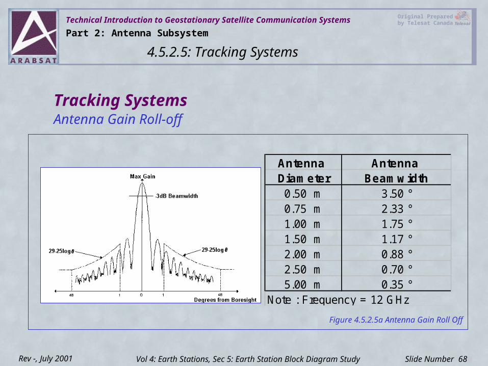
Antenna gain decreases as the mispointing angle increases. This loss of signal is directly related to its size and half power beamwidths (-3dB points).
Tracking Systems
Part 2: Antenna Subsystem
4.5.2.5: Tracking Systems
Vol 4: Earth Stations, Sec 5: Earth Station Block Diagram Study
Technical Introduction to Geostationary Satellite Communication Systems Original Prepared by Telesat Canada
Slide Number 68Rev -, July 2001
Antenna Gain Roll-offTracking Systems
Part 2: Antenna Subsystem
4.5.2.5: Tracking Systems
Vol 4: Earth Stations, Sec 5: Earth Station Block Diagram Study
Antenna Antenna Diameter Beamwidth
0.50 m 3.50 °0.75 m 2.33 °1.00 m 1.75 °1.50 m 1.17 °2.00 m 0.88 °2.50 m 0.70 °5.00 m 0.35 °
Note : Frequency = 12 GHz
Figure 4.5.2.5a Antenna Gain Roll Off
Technical Introduction to Geostationary Satellite Communication Systems Original Prepared by Telesat Canada
Slide Number 69Rev -, July 2001
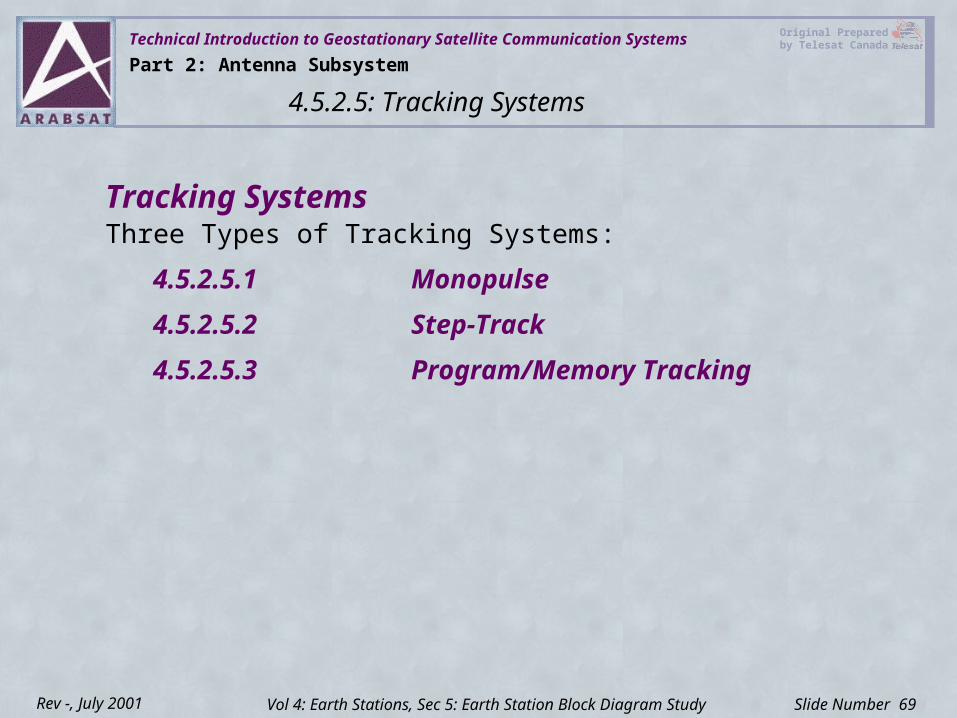
Three Types of Tracking Systems:
4.5.2.5.1 Monopulse
4.5.2.5.2 Step-Track
4.5.2.5.3 Program/Memory Tracking
Tracking Systems
Part 2: Antenna Subsystem
4.5.2.5: Tracking Systems
Vol 4: Earth Stations, Sec 5: Earth Station Block Diagram Study
Technical Introduction to Geostationary Satellite Communication Systems Original Prepared by Telesat Canada
Slide Number 70Rev -, July 2001
4.5.2.5.1MonopulseMonopulse derives its name from radar technology.
During the early stages of satellite communications, monopulse tracking of one form or another was used almost exclusively. From the mid 1970’s to present, there has been a shift towards the use of step-track auto-tracking systems.
Monopulse tracking requires an antenna built with a special antenna feed.
Antenna orientation command signals are generated by a monopulse tracking receiver. The receiver performs a comparison of a reference signal and the error angle measurement signal caused by azimuth and elevation misalignments.
Part 2: Antenna Subsystem
4.5.2.5: Tracking Systems
Vol 4: Earth Stations, Sec 5: Earth Station Block Diagram Study
Technical Introduction to Geostationary Satellite Communication Systems Original Prepared by Telesat Canada
Slide Number 71Rev -, July 2001
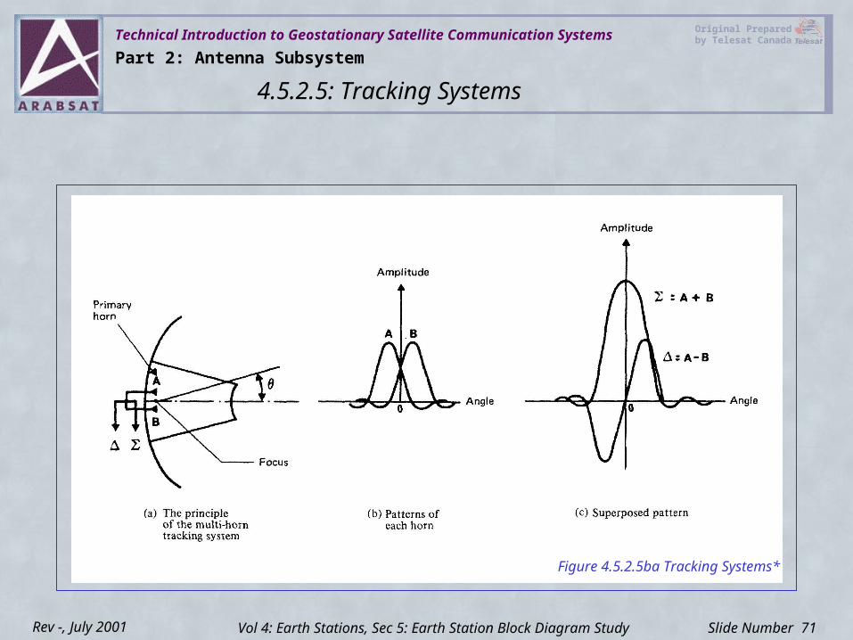
Figure 4.5.2.5ba Tracking Systems*
Part 2: Antenna Subsystem
4.5.2.5: Tracking Systems
Vol 4: Earth Stations, Sec 5: Earth Station Block Diagram Study
Technical Introduction to Geostationary Satellite Communication Systems Original Prepared by Telesat Canada
Slide Number 72Rev -, July 2001
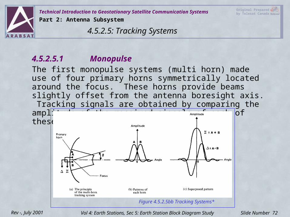
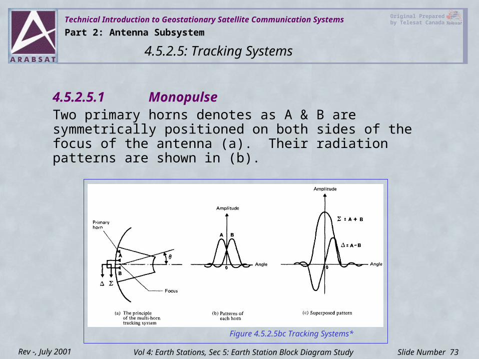
4.5.2.5.1MonopulseThe first monopulse systems (multi horn) made use of four primary horns symmetrically located around the focus. These horns provide beams slightly offset from the antenna boresight axis. Tracking signals are obtained by comparing the amplitude of the received signals of each of these beams.
Part 2: Antenna Subsystem
4.5.2.5: Tracking Systems
Vol 4: Earth Stations, Sec 5: Earth Station Block Diagram Study
Figure 4.5.2.5bb Tracking Systems*
Technical Introduction to Geostationary Satellite Communication Systems Original Prepared by Telesat Canada
Slide Number 73Rev -, July 2001
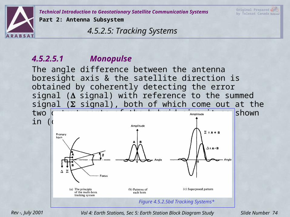
4.5.2.5.1MonopulseTwo primary horns denotes as A & B are symmetrically positioned on both sides of the focus of the antenna (a). Their radiation patterns are shown in (b).
Part 2: Antenna Subsystem
4.5.2.5: Tracking Systems
Vol 4: Earth Stations, Sec 5: Earth Station Block Diagram Study
Figure 4.5.2.5bc Tracking Systems*
Technical Introduction to Geostationary Satellite Communication Systems Original Prepared by Telesat Canada
Slide Number 74Rev -, July 2001
4.5.2.5.1MonopulseThe angle difference between the antenna boresight axis & the satellite direction is obtained by coherently detecting the error signal (signal) with reference to the summed signal ( signal), both of which come out at the two output ports of the hybrid circuit as shown in (c).
Part 2: Antenna Subsystem
4.5.2.5: Tracking Systems
Vol 4: Earth Stations, Sec 5: Earth Station Block Diagram Study
Figure 4.5.2.5bd Tracking Systems*
Technical Introduction to Geostationary Satellite Communication Systems Original Prepared by Telesat Canada
Slide Number 75Rev -, July 2001
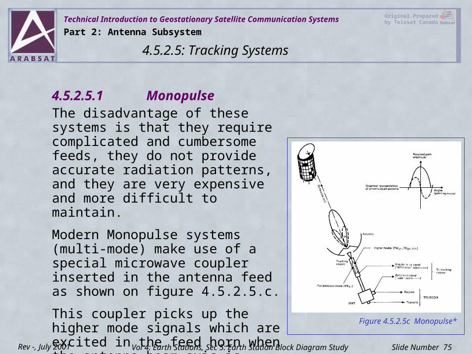
4.5.2.5.1MonopulseThe disadvantage of these systems is that they require complicated and cumbersome feeds, they do not provide accurate radiation patterns, and they are very expensive and more difficult to maintain.
Modern Monopulse systems (multi-mode) make use of a special microwave coupler inserted in the antenna feed as shown on figure 4.5.2.5.c.
This coupler picks up the higher mode signals which are excited in the feed horn when the antenna beam axis is offset from the satellite direction.
Part 2: Antenna Subsystem
4.5.2.5: Tracking Systems
Vol 4: Earth Stations, Sec 5: Earth Station Block Diagram Study
Figure 4.5.2.5c Monopulse*
Technical Introduction to Geostationary Satellite Communication Systems Original Prepared by Telesat Canada
Slide Number 76Rev -, July 2001
4.5.2.5.1MonopulseSuch higher mode signals correspond to odd mode radiation patterns with a null in the beam axis direction.
After coherent detection by a reference signal (which is the normal fundamental mode signal), bipolar discrimination error voltages are obtained and are directly fed to the servo system that controls antenna motion.
When operating in circular mode, only one higher odd mode of circular waveguide is required (TM01). This is because both the phase and amplitude of the TM01 component, when compared with the fundamental TE11 (used as reference), bears angular error information.
Part 2: Antenna Subsystem
4.5.2.5: Tracking Systems
Vol 4: Earth Stations, Sec 5: Earth Station Block Diagram Study
Technical Introduction to Geostationary Satellite Communication Systems Original Prepared by Telesat Canada
Slide Number 77Rev -, July 2001
4.5.2.5.1MonopulseWhen operating in linear polarization mode, TM01 detection only delivers one error signal (e.g. Azimuth) and a second higher odd mode is required for elevation. This second mode can be the TE01 mode.
Combination of other modes is possible (e.g. TE21 with proper orientation or TM01 + TE21 etc.). In this case the tracking receiver will need to accept two input error signals as opposed to one error signal for circular.
Part 2: Antenna Subsystem
4.5.2.5: Tracking Systems
Vol 4: Earth Stations, Sec 5: Earth Station Block Diagram Study
Technical Introduction to Geostationary Satellite Communication Systems Original Prepared by Telesat Canada
Slide Number 78Rev -, July 2001
4.5.2.5.2Step-TrackWith the continuous improvement in station keeping accuracy of GEO satellites, a much less complex and lower cost step-track system was developed.
Monopulse tracking systems, although very accurate, have largely been replaced by step-track systems because of their lower cost, greater simplicity, and easier maintenance.
The step track method uses a so called “climbing the hill method”. The antenna beam is steered step by step so as to obtain stronger receive signal from the satellite than was obtained in the last step.
If the step steering of the antenna beam has decreased the receive signal level, the step track processor will command the antenna to be steered in the opposite direction.
Part 2: Antenna Subsystem
4.5.2.5: Tracking Systems
Vol 4: Earth Stations, Sec 5: Earth Station Block Diagram Study
Technical Introduction to Geostationary Satellite Communication Systems Original Prepared by Telesat Canada
Slide Number 79Rev -, July 2001
4.5.2.5.2Step-TrackThe receive signal is usually derived from a satellite beacon carrier.
In the step-track system, no special tracking feed is required. Only a simple beacon receiver and step track processor is necessary.
A disadvantage of the step-track system is that the tracking accuracy is directly affected by rapid variations of the incoming signal due to atmospheric disturbances such as wind, rain absorption and beacon instability.
These limitations can be overcome by choosing a step size that is sufficiently small, but not so small as to cause the antenna to continuously hunt for the satellite as, for example, during moderate wind loading conditions.
Part 2: Antenna Subsystem
4.5.2.5: Tracking Systems
Vol 4: Earth Stations, Sec 5: Earth Station Block Diagram Study
Technical Introduction to Geostationary Satellite Communication Systems Original Prepared by Telesat Canada
Slide Number 80Rev -, July 2001
4.5.2.5.3Program/Memory TrackingWhen considering inclined orbit satellites a programmed tracking system becomes more attractive.
The antenna is controlled by a computer/software combination. Calculation of satellite orbital position is derived from pointing data (11 ephemeris parameters), thus eliminating the need for a satellite beacon.
Another option is the so called “Smooth Step-Track” system that memorizes the satellite’s track within the first 24 hours of acquisition. Then it follows the memorized program from the previous day. This feature would not be recommended for inclined orbit satellites.
Part 2: Antenna Subsystem
4.5.2.5: Tracking Systems
Vol 4: Earth Stations, Sec 5: Earth Station Block Diagram Study
Technical Introduction to Geostationary Satellite Communication Systems Original Prepared by Telesat Canada
Slide Number 81Rev -, July 2001
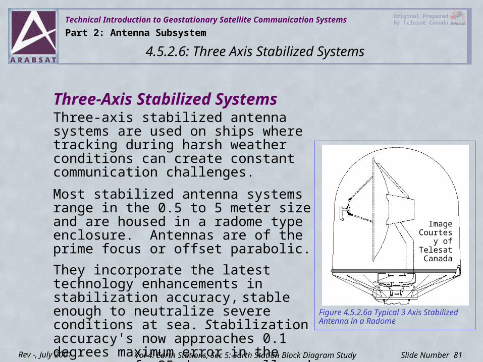
Three-Axis Stabilized SystemsThree-axis stabilized antenna systems are used on ships where tracking during harsh weather conditions can create constant communication challenges.
Most stabilized antenna systems range in the 0.5 to 5 meter size and are housed in a radome type enclosure. Antennas are of the prime focus or offset parabolic.They incorporate the latest technology enhancements in stabilization accuracy, stable enough to neutralize severe conditions at sea. Stabilization accuracy's now approaches 0.1 degrees maximum error in the presence of +25 degrees roll and + 15 degrees pitch.
Part 2: Antenna Subsystem
4.5.2.6: Three Axis Stabilized Systems
Vol 4: Earth Stations, Sec 5: Earth Station Block Diagram Study
Figure 4.5.2.6a Typical 3 Axis Stabilized Antenna in a Radome
Image Courtesy
of Telesat Canada
Technical Introduction to Geostationary Satellite Communication Systems Original Prepared by Telesat Canada
Slide Number 82Rev -, July 2001
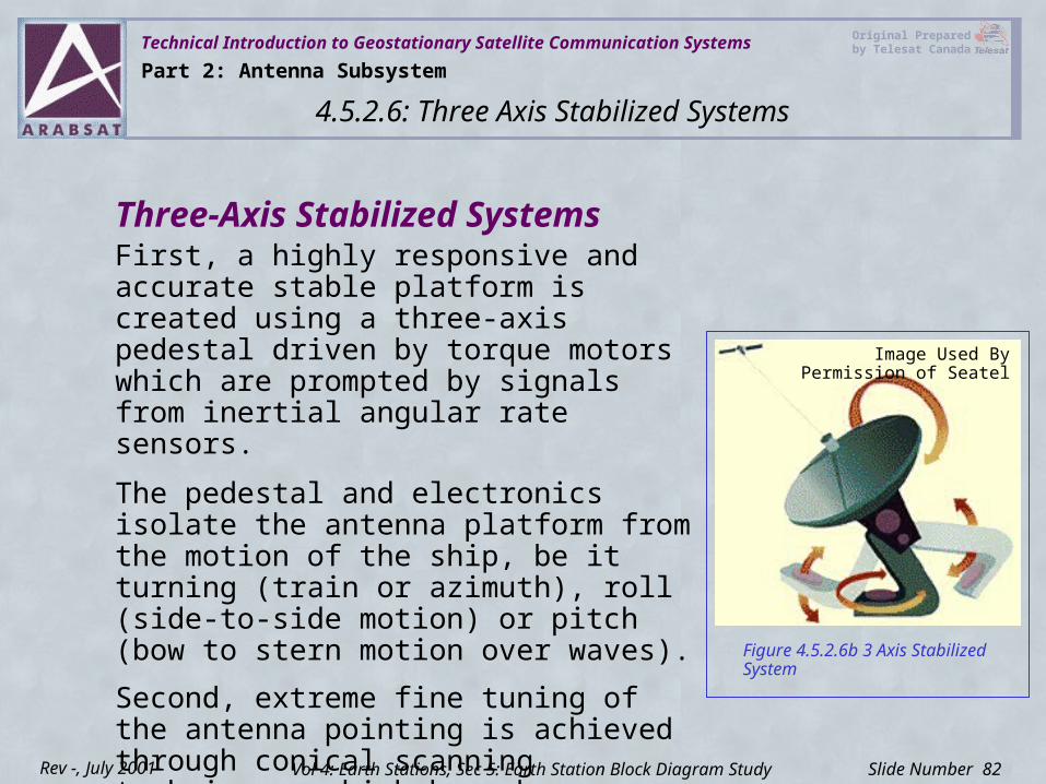
Three-Axis Stabilized SystemsFirst, a highly responsive and accurate stable platform is created using a three-axis pedestal driven by torque motors which are prompted by signals from inertial angular rate sensors.
The pedestal and electronics isolate the antenna platform from the motion of the ship, be it turning (train or azimuth), roll (side-to-side motion) or pitch (bow to stern motion over waves).
Second, extreme fine tuning of the antenna pointing is achieved through conical scanning techniques, which have been implemented by using digital signal processing.
Part 2: Antenna Subsystem
4.5.2.6: Three Axis Stabilized Systems
Vol 4: Earth Stations, Sec 5: Earth Station Block Diagram Study
Figure 4.5.2.6b 3 Axis Stabilized System
Image Used By Permission of Seatel
Technical Introduction to Geostationary Satellite Communication Systems Original Prepared by Telesat Canada
Slide Number 83Rev -, July 2001
Three-Axis Stabilized SystemsUtilizing modern conical scan tracking, the antenna control unit senses and compares the signal levels in all four of the antenna quadrants (up, down, left and right).
It then quickly and smoothly adjusts the antenna in elevation and azimuth to equalize the signal strength in each quadrant, which translates to extremely accurate pointing to the source of the signal, the satellite.
Conical scanning has been around since World War II radar and is considered the superior method of signal tracking for satellite communications three axis stabilized systems.
Part 2: Antenna Subsystem
4.5.2.6: Three Axis Stabilized Systems
Vol 4: Earth Stations, Sec 5: Earth Station Block Diagram Study
Technical Introduction to Geostationary Satellite Communication Systems Original Prepared by Telesat Canada
Slide Number 84Rev -, July 2001
De-icing EquipmentThe purpose of a de-ice system is to melt away any snow or ice accumulation building up on a parabolic reflector caused by snow or freezing rain.
Ku-Band signals are more susceptible to snow build up than is C-Band but in either case a large buildup will reduce the antenna gain and may cause service degradation.
De-icing equipment can be purchased in 2 ways:
• Purchased with the antenna at time of ordering (factory Installed)
• Purchased as a add-on if the original antenna installed was not equipped with de-icing
Part 2: Antenna Subsystem
4.5.2.7: De-icing Equipment
Vol 4: Earth Stations, Sec 5: Earth Station Block Diagram Study
Technical Introduction to Geostationary Satellite Communication Systems Original Prepared by Telesat Canada
Slide Number 85Rev -, July 2001
De-icing EquipmentDe-icing comes in various types based on the energy source used to create the heat required for the de-ice elements:
• Electrical-elements
• Electrical-Hot air blowers
• Gas
• Propane
Part 2: Antenna Subsystem
4.5.2.7: De-icing Equipment
Vol 4: Earth Stations, Sec 5: Earth Station Block Diagram Study
Technical Introduction to Geostationary Satellite Communication Systems Original Prepared by Telesat Canada
Slide Number 86Rev -, July 2001
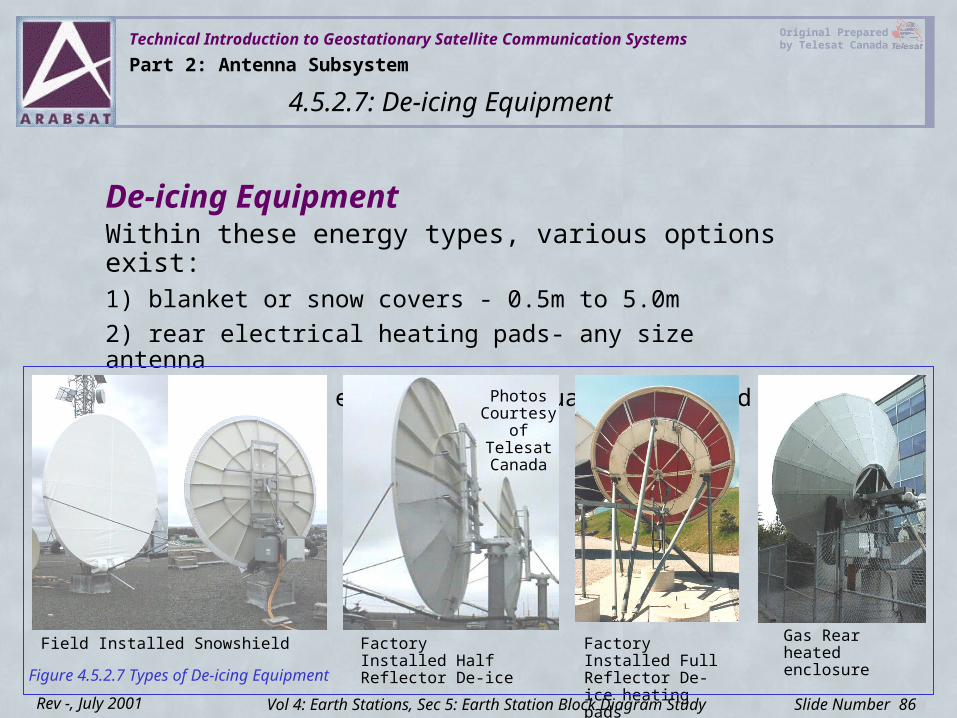
De-icing EquipmentWithin these energy types, various options exist: 1) blanket or snow covers - 0.5m to 5.0m2) rear electrical heating pads- any size antenna3) rear heating enclosures - usually 4.5m and up
Field Installed Snowshield Factory Installed Full Reflector De-ice heating pads
Factory Installed Half Reflector De-ice
Gas Rear heated enclosure
Part 2: Antenna Subsystem
4.5.2.7: De-icing Equipment
Vol 4: Earth Stations, Sec 5: Earth Station Block Diagram Study
Figure 4.5.2.7 Types of De-icing Equipment
Photos Courtesy
of Telesat Canada
Technical Introduction to Geostationary Satellite Communication Systems Original Prepared by Telesat Canada
Slide Number 87Rev -, July 2001
De-icing EquipmentA de-icing system consists of a control unit, a thermostat and some type of heating element. Some units add more complexity by adding a moisture sensor.
Most units will automatically turn on if the temperature goes below about 3C. Or, if equipped with a moisture sensor, then the units will require both a temperature below 3C and the presence of moisture before turning on.
Still others will deactivate the heating elements, even when moisture is present, if the temperature goes below -9C. This is based on the principle that below -9C the precipitation is sure to be snow and conditions do not favor a buildup on the antenna.
De-icing draws a lot of power, so if power saving is critical, then a moisture sensor is a must for a de-ice system. De-icing is highly recommended for large antenna systems.
Part 2: Antenna Subsystem
4.5.2.7: De-icing Equipment
Vol 4: Earth Stations, Sec 5: Earth Station Block Diagram Study
Technical Introduction to Geostationary Satellite Communication Systems Original Prepared by Telesat Canada
Slide Number 88Rev -, July 2001
De-icing Equipment
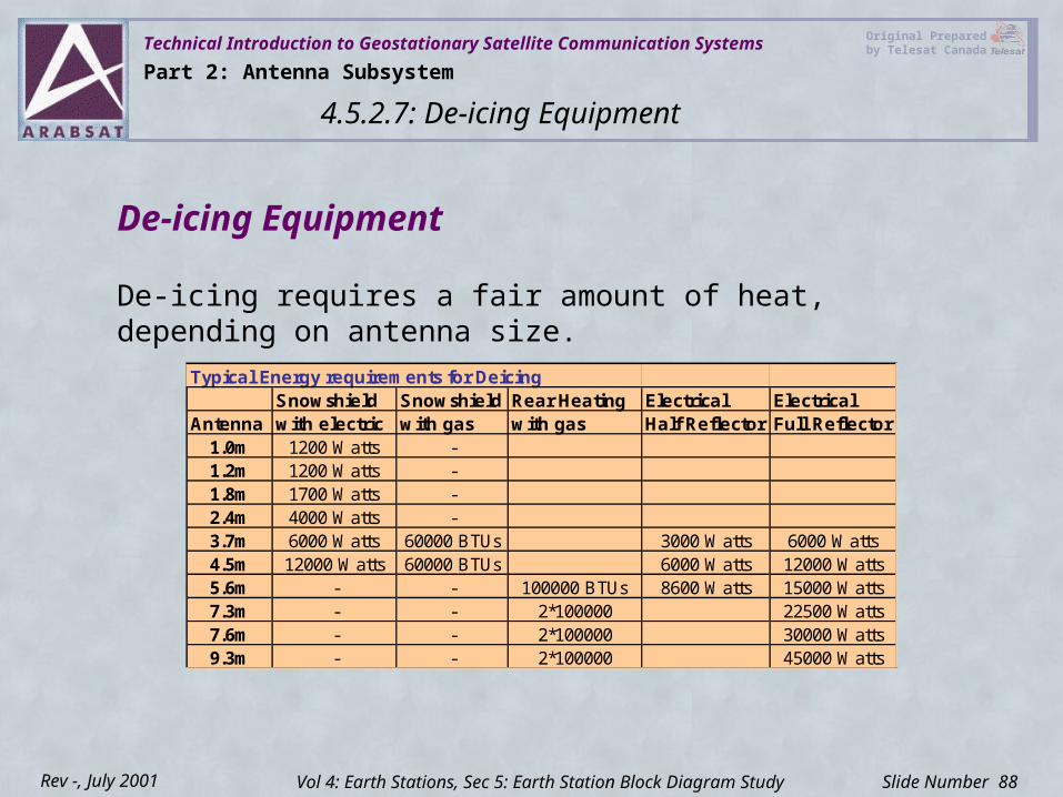
De-icing requires a fair amount of heat, depending on antenna size.
Typical Energy requirements for DeicingSnowshield Snowshield Rear Heating Electrical Electrical
Antenna with electric with gas with gas Half Reflector Full Reflector1.0m 1200 Watts -1.2m 1200 Watts -1.8m 1700 Watts -2.4m 4000 Watts -3.7m 6000 Watts 60000 BTUs 3000 Watts 6000 Watts4.5m 12000 Watts 60000 BTUs 6000 Watts 12000 Watts5.6m - - 100000 BTUs 8600 Watts 15000 Watts7.3m - - 2*100000 22500 Watts7.6m - - 2*100000 30000 Watts9.3m - - 2*100000 45000 Watts
Part 2: Antenna Subsystem
4.5.2.7: De-icing Equipment
Vol 4: Earth Stations, Sec 5: Earth Station Block Diagram Study
Technical Introduction to Geostationary Satellite Communication Systems Original Prepared by Telesat Canada
Slide Number 89Rev -, July 2001
4.5: Earth Station Block Diagram StudyVol 4: Earth Stations
Low Noise AmplifiersPart 3
Technical Introduction to Geostationary Satellite Communication Systems Original Prepared by Telesat Canada
Slide Number 90Rev -, July 2001
Contents
Sec 5: Earth Stations Block Diagram Study
4.5.3.1 LNA4.5.3.2 LNB4.5.3.3 LNC4.5.3.4 LNB-F
4.5.3: Low Noise Amplifiers
Vol 4: Earth Stations
Technical Introduction to Geostationary Satellite Communication Systems Original Prepared by Telesat Canada
Slide Number 91Rev -, July 2001
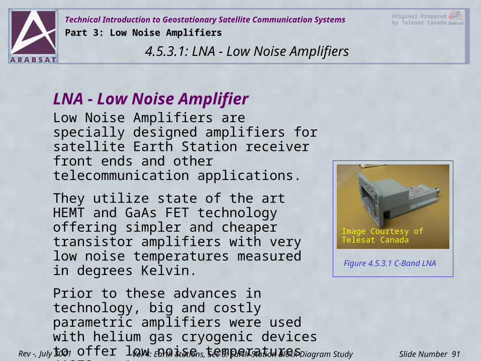
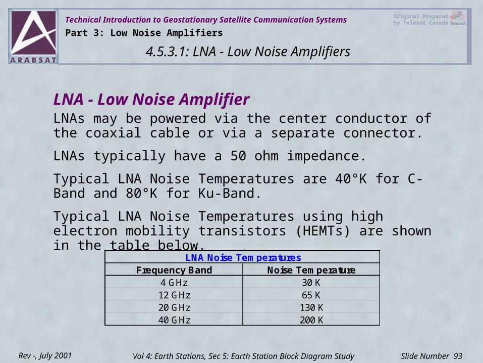
LNA - Low Noise Amplifier
Part 3: Low Noise Amplifiers
Low Noise Amplifiers are specially designed amplifiers for satellite Earth Station receiver front ends and other telecommunication applications.
They utilize state of the art HEMT and GaAs FET technology offering simpler and cheaper transistor amplifiers with very low noise temperatures measured in degrees Kelvin.
Prior to these advances in technology, big and costly parametric amplifiers were used with helium gas cryogenic devices to offer low noise temperatures (1970 era).
4.5.3.1: LNA - Low Noise Amplifiers
Vol 4: Earth Stations, Sec 5: Earth Station Block Diagram Study
Figure 4.5.3.1 C-Band LNA
Image Courtesy of Telesat Canada
Technical Introduction to Geostationary Satellite Communication Systems Original Prepared by Telesat Canada
Slide Number 92Rev -, July 2001
LNA - Low Noise AmplifierThe radio signal entering the Earth Station Antenna is a very low level, weak signal. The LNA is a highly sensitive preamplifier with very low thermal noise. LNA’s are wideband devices amplifying 500 MHz to 1 GHz of bandwidth.
For satellite system front ends, the lower the noise temperature the better, as noise temperature greatly influences the very important G/T parameter of the receiving Earth Station.
It is the antenna and LNA that characterize the G/T, the ratio of the antenna gain to the total noise temperature of the LNA and antenna system.
LNA’s should be placed as close as possible to the antenna feed, to avoid additional contributions of noise caused by waveguide losses.
Part 3: Low Noise Amplifiers
4.5.3.1: LNA - Low Noise Amplifiers
Vol 4: Earth Stations, Sec 5: Earth Station Block Diagram Study
Technical Introduction to Geostationary Satellite Communication Systems Original Prepared by Telesat Canada
Slide Number 93Rev -, July 2001
Frequency Band Noise Temperature4 GHz 30 K12 GHz 65 K20 GHz 130 K40 GHz 200 K
LNA Noise Temperatures
Part 3: Low Noise Amplifiers
4.5.3.1: LNA - Low Noise Amplifiers
Vol 4: Earth Stations, Sec 5: Earth Station Block Diagram Study
LNA - Low Noise AmplifierLNAs may be powered via the center conductor of the coaxial cable or via a separate connector.
LNAs typically have a 50 ohm impedance.
Typical LNA Noise Temperatures are 40°K for C-Band and 80°K for Ku-Band.
Typical LNA Noise Temperatures using high electron mobility transistors (HEMTs) are shown in the table below.
Technical Introduction to Geostationary Satellite Communication Systems Original Prepared by Telesat Canada
Slide Number 94Rev -, July 2001
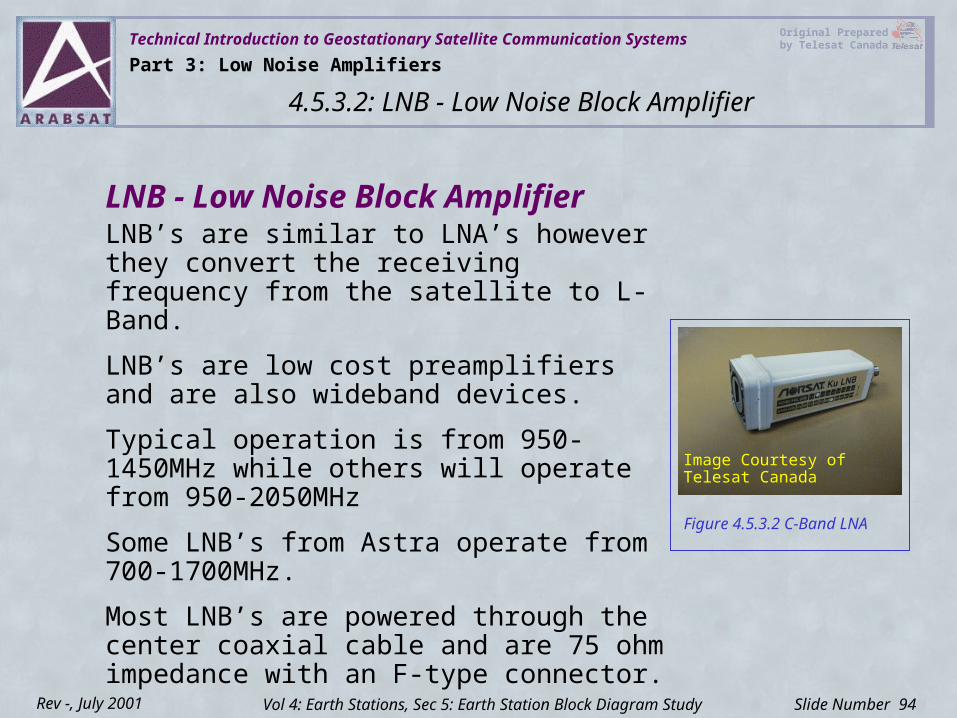
LNB - Low Noise Block AmplifierLNB’s are similar to LNA’s however they convert the receiving frequency from the satellite to L-Band.
LNB’s are low cost preamplifiers and are also wideband devices.
Typical operation is from 950-1450MHz while others will operate from 950-2050MHz
Some LNB’s from Astra operate from 700-1700MHz.
Most LNB’s are powered through the center coaxial cable and are 75 ohm impedance with an F-type connector.
Part 3: Low Noise Amplifiers
4.5.3.2: LNB - Low Noise Block Amplifier
Vol 4: Earth Stations, Sec 5: Earth Station Block Diagram Study
Figure 4.5.3.2 C-Band LNA
Image Courtesy of Telesat Canada
Technical Introduction to Geostationary Satellite Communication Systems Original Prepared by Telesat Canada
Slide Number 95Rev -, July 2001
LNC - Low Noise ConverterLNC’s have no distinguishable difference from an LNB other than they may output a different frequency, from 2 GHz to 70 MHz.
Some LNC’s may have external LO inputs for greater accuracy in the frequency downconversion process.
Part 3: Low Noise Amplifiers
4.5.3.3: LNC - Low Noise Converter
Vol 4: Earth Stations, Sec 5: Earth Station Block Diagram Study
Technical Introduction to Geostationary Satellite Communication Systems Original Prepared by Telesat Canada
Slide Number 96Rev -, July 2001
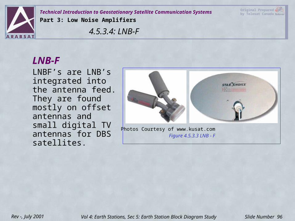
LNB-FLNBF’s are LNB’s integrated into the antenna feed.They are found mostly on offset antennas and small digital TV antennas for DBS satellites. Figure 4.5.3.3 LNB - F
Photos Courtesy of www.kusat.com
Part 3: Low Noise Amplifiers
4.5.3.4: LNB-F
Vol 4: Earth Stations, Sec 5: Earth Station Block Diagram Study
Technical Introduction to Geostationary Satellite Communication Systems Original Prepared by Telesat Canada
Slide Number 97Rev -, July 2001
4.5: Earth Station Block Diagram StudyVol 4: Earth Stations
High Power Amplifiers (HPA)Part 4
Technical Introduction to Geostationary Satellite Communication Systems Original Prepared by Telesat Canada
Slide Number 98Rev -, July 2001
Contents
Sec 5: Earth Stations Block Diagram Study
4.5.4.1 Klystron4.5.4.2 Travelling Wave Tube4.5.4.3 Solid State Power Amplifier (SSPA)4.5.4.4 Comparison of all 3 types
4.5.4: High Power Amplifiers (HPA)
Vol 4: Earth Stations
Technical Introduction to Geostationary Satellite Communication Systems Original Prepared by Telesat Canada
Slide Number 99Rev -, July 2001
Klystron
Part 4: High Power Amplifiers (HPA)
Description
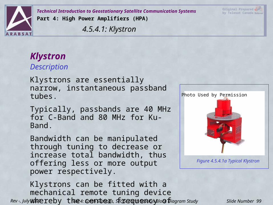
Klystrons are essentially narrow, instantaneous passband tubes.
Typically, passbands are 40 MHz for C-Band and 80 MHz for Ku-Band.
Bandwidth can be manipulated through tuning to decrease or increase total bandwidth, thus offering less or more output power respectively.
Klystrons can be fitted with a mechanical remote tuning device whereby the center frequency of the passband can be changed.
4.5.4.1: Klystron
Vol 4: Earth Stations, Sec 5: Earth Station Block Diagram Study
Figure 4.5.4.1a Typical Klystron
Photo Used by Permission
Technical Introduction to Geostationary Satellite Communication Systems Original Prepared by Telesat Canada
Slide Number 100Rev -, July 2001
Klystron A Klystron consists of:
• A series of cavities (usually five) which are microwave resonant circuits traversed by a electron beam
• Electron Gun
• Collector
• Focusing Magnet
• Beam, Heater & Low Voltage Power Supplies
• Cooling Equipment
• Monitor and Control Logic
Part 4: High Power Amplifiers (HPA)
4.5.4.1: Klystron
Vol 4: Earth Stations, Sec 5: Earth Station Block Diagram Study
Technical Introduction to Geostationary Satellite Communication Systems Original Prepared by Telesat Canada
Slide Number 101Rev -, July 2001
KlystronEach cavity is individually tuned, and electromagnets are placed between cavities for focusing purposes.
In the first cavity (the input cavity), the traversing electron beam is excited by the microwave signal that is to be amplified. This generates an alternating signal across the gap of the cavity. The velocity of the electrons passing through the beam will be modulated with the RF input signal.
Each of the cavities are successively tuned in such a way as to reproduce a linear amplified input signal. In the output cavity, the RF output signal is coupled to the transmission line and antenna (load).
Part 4: High Power Amplifiers (HPA)
4.5.4.1: Klystron
Vol 4: Earth Stations, Sec 5: Earth Station Block Diagram Study
Technical Introduction to Geostationary Satellite Communication Systems Original Prepared by Telesat Canada
Slide Number 102Rev -, July 2001
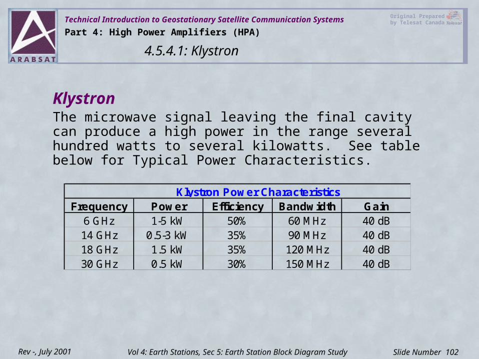
Frequency Power Efficiency Bandwidth Gain6 GHz 1-5 kW 50% 60 MHz 40 dB14 GHz 0.5-3 kW 35% 90 MHz 40 dB18 GHz 1.5 kW 35% 120 MHz 40 dB30 GHz 0.5 kW 30% 150 MHz 40 dB
Klystron Power Characteristics
KlystronThe microwave signal leaving the final cavity can produce a high power in the range several hundred watts to several kilowatts. See table below for Typical Power Characteristics.
Part 4: High Power Amplifiers (HPA)
4.5.4.1: Klystron
Vol 4: Earth Stations, Sec 5: Earth Station Block Diagram Study
Technical Introduction to Geostationary Satellite Communication Systems Original Prepared by Telesat Canada
Slide Number 103Rev -, July 2001
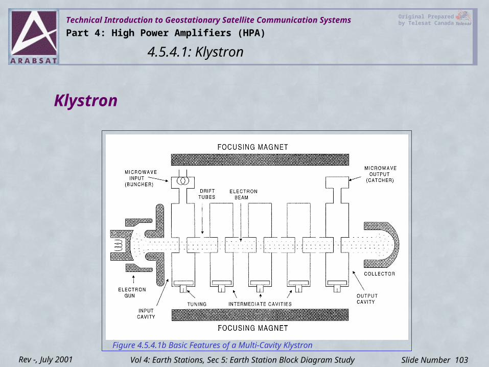
Klystron
Figure 4.5.4.1b Basic Features of a Multi-Cavity Klystron
Part 4: High Power Amplifiers (HPA)
4.5.4.1: Klystron
Vol 4: Earth Stations, Sec 5: Earth Station Block Diagram Study
Technical Introduction to Geostationary Satellite Communication Systems Original Prepared by Telesat Canada
Slide Number 104Rev -, July 2001
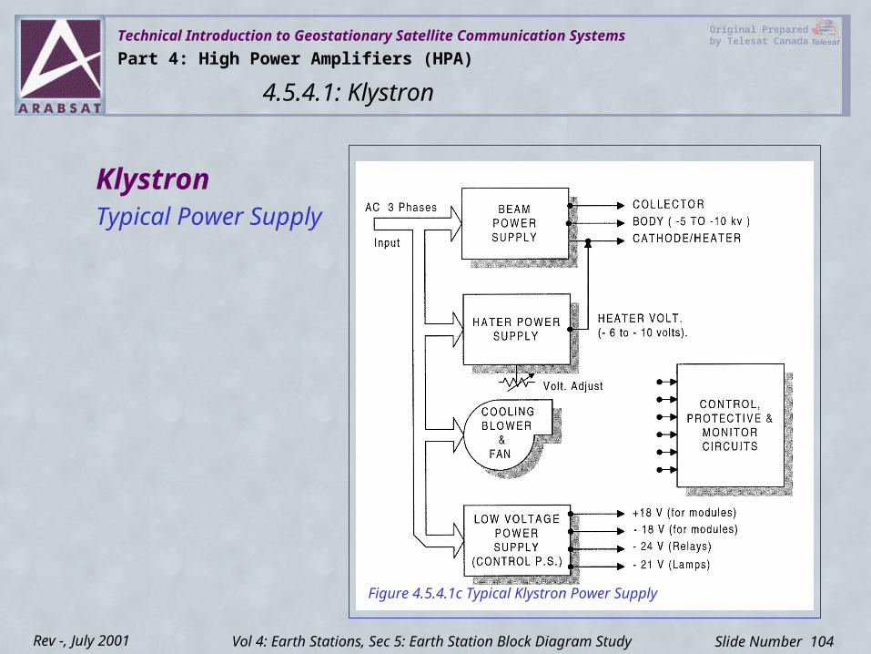
KlystronTypical Power Supply
Figure 4.5.4.1c Typical Klystron Power Supply
Part 4: High Power Amplifiers (HPA)
4.5.4.1: Klystron
Vol 4: Earth Stations, Sec 5: Earth Station Block Diagram Study
Technical Introduction to Geostationary Satellite Communication Systems Original Prepared by Telesat Canada
Slide Number 105Rev -, July 2001
KlystronMost Common Klystron Faults
Several faults can appear on a Klystron. Any fault should be considered serious, as Klystrons are very expensive to repair.
• Air flow alarms - usually a wind vane or blower is faulty, or a wind vane could be incorrectly set. A Klystron could have multiple air return systems so all would need to be checked.
• High temp alarm - usually an air blower has failed, or the air plenum return attachment has not been fitted properly or has fallen loose from the Klystron collector, or AC phases are incorrectly connected to the air blowers (need to be reversed).
Part 4: High Power Amplifiers (HPA)
4.5.4.1: Klystron
Vol 4: Earth Stations, Sec 5: Earth Station Block Diagram Study
Technical Introduction to Geostationary Satellite Communication Systems Original Prepared by Telesat Canada
Slide Number 106Rev -, July 2001
KlystronMost Common Klystron Faults
• High body current - tube has gotten gassy, been turned off too long (more than 6 months), or the cavities are not tuned properly, or a cavity is faulty. Beam power supply should be operating at correct voltage.
• Arc detector - if an arc has been detected inside the klystron output waveguide assembly, this would be caused by a mismatch in the waveguide impedance due to high VSWR.
Part 4: High Power Amplifiers (HPA)
4.5.4.1: Klystron
Vol 4: Earth Stations, Sec 5: Earth Station Block Diagram Study
Technical Introduction to Geostationary Satellite Communication Systems Original Prepared by Telesat Canada
Slide Number 107Rev -, July 2001
KlystronTypes of Distortion
HarmonicsAs a Klystron is backed away from saturation, the carrier to product ratio improves. However when the tube is driven near saturation or beyond, harmonic components increase.
Because the electron bunches passing through the cavity occur in quick “kicks”, it is evident that the output current may not be purely sinusoidal and will, therefore, contain harmonic components.
Harmonic suppression filters are often used to reduce this intermodulation level to -50 to -60 dB.
Part 4: High Power Amplifiers (HPA)
4.5.4.1: Klystron
Vol 4: Earth Stations, Sec 5: Earth Station Block Diagram Study
Technical Introduction to Geostationary Satellite Communication Systems Original Prepared by Telesat Canada
Slide Number 108Rev -, July 2001
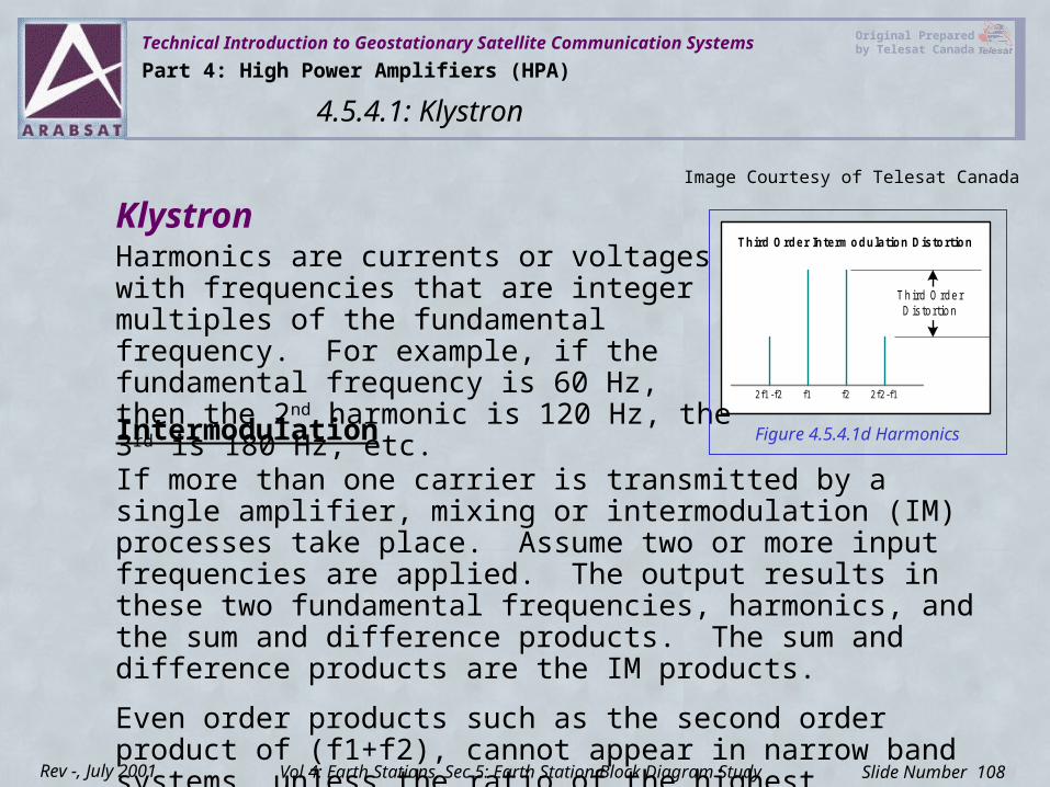
Klystron
IntermodulationIf more than one carrier is transmitted by a single amplifier, mixing or intermodulation (IM) processes take place. Assume two or more input frequencies are applied. The output results in these two fundamental frequencies, harmonics, and the sum and difference products. The sum and difference products are the IM products.
Even order products such as the second order product of (f1+f2), cannot appear in narrow band systems, unless the ratio of the highest frequency (f2) to the lowest frequency (f1) is at least 2 to 1.
2f1-f2 f1 2f2-f1f2
Third O rderD istortion
T hird O rder Interm od ulation DistortionHarmonics are currents or voltages with frequencies that are integer multiples of the fundamental frequency. For example, if the fundamental frequency is 60 Hz, then the 2nd harmonic is 120 Hz, the 3rd is 180 Hz, etc.
Figure 4.5.4.1d Harmonics
Image Courtesy of Telesat Canada
Part 4: High Power Amplifiers (HPA)
4.5.4.1: Klystron
Vol 4: Earth Stations, Sec 5: Earth Station Block Diagram Study
Technical Introduction to Geostationary Satellite Communication Systems Original Prepared by Telesat Canada
Slide Number 109Rev -, July 2001
KlystronOdd order products such as the third order distortion products of 2f1-f2 or 2f2-f1 are the most significant IM products appearing in the frequency band regardless of the frequency ratio.
AM/PM Conversion
AM/PM conversion is defined as the change in phase angle of the output RF voltage produced by variations in input signal level. AM/PM is expressed in degrees per decibel and must always be defined at a specific power level. The slope of the curve relating output phase (in degrees) to drive level (in decibels) is very small for very small signals, but the slope begins to increase when the input signal is increased as saturation is approached.
The principal reason that AM/PM occurs in a microwave Vacuum Electron Device (VED) is because average beam velocity decreases as the input is amplified.
Part 4: High Power Amplifiers (HPA)
4.5.4.1: Klystron
Vol 4: Earth Stations, Sec 5: Earth Station Block Diagram Study
Technical Introduction to Geostationary Satellite Communication Systems Original Prepared by Telesat Canada
Slide Number 110Rev -, July 2001
KlystronThis decrease in beam velocity is due to the energy exchange between the beam and the growing RF wave, and this results in increased electrical length of the VED.
Group delayIn an ideal transmission system, the phase shift of any signal component is directly proportional to frequency, but in most systems, phase distortions can occur due to mechanical imperfections and resonant cavity filter effects.
In systems, a point of interest is the relative group delay in a particular passband of frequencies around the radiated microwave carrier. In the Klystron amplifier, group delay characteristics as well as gain, gain slope, and passband ripple are all dependent upon the tuning of the Klystron. With the use of channel tuning, a particular characteristic, once attained, is always recoverable at will.
Part 4: High Power Amplifiers (HPA)
4.5.4.1: Klystron
Vol 4: Earth Stations, Sec 5: Earth Station Block Diagram Study
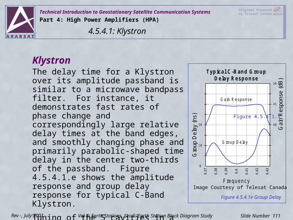
Technical Introduction to Geostationary Satellite Communication Systems Original Prepared by Telesat Canada
Slide Number 111Rev -, July 2001
KlystronThe delay time for a Klystron over its amplitude passband is similar to a microwave bandpass filter. For instance, it demonstrates fast rates of phase change and correspondingly large relative delay times at the band edges, and smoothly changing phase and primarily parabolic-shaped time delay in the center two-thirds of the passband. Figure 4.5.4.1.e shows the amplitude response and group delay response for typical C-Band Klystron.
Tuning of the 5 cavities in a Klystron affect the group delay characteristics.
0
10
20
6.37
Gro
up D
elay
(ns)
Gain Response
G roup Delay
6.38
6.39 6.4
6.41
6.42
6.43
Frequency
Typical C-Band GroupDelay Response
40
45
Gai
n R
espo
nse
(dB
)
50
Figure 4.5.4.1.1
Figure 4.5.4.1e Group Delay
Image Courtesy of Telesat Canada
Part 4: High Power Amplifiers (HPA)
4.5.4.1: Klystron
Vol 4: Earth Stations, Sec 5: Earth Station Block Diagram Study
Technical Introduction to Geostationary Satellite Communication Systems Original Prepared by Telesat Canada
Slide Number 112Rev -, July 2001
KlystronNoise
A klystron, like any other electron tube, generates a certain amount of “white noise”. White noise occurs because an electron beam is never perfectly uniform. A typical Noise Figure for a Klystron is 31 dB.
Additionally, noise power density is described in terms of dBm/kHz and is affected by Klystron Gain, Noise Figure and the transmission bandwidth.
Part 4: High Power Amplifiers (HPA)
4.5.4.1: Klystron
Vol 4: Earth Stations, Sec 5: Earth Station Block Diagram Study
Technical Introduction to Geostationary Satellite Communication Systems Original Prepared by Telesat Canada
Slide Number 113Rev -, July 2001
KlystronSpurious Output NoiseSystem specifications often lump noise power output and spurious outputs together.
Spurious outputs are defined as discrete frequency components excluding AM and FM spectral lines and their harmonics. Spurious modulation resulting from atomic oscillation of residual ions are often included in the broad category of noise. In the sense that these signals are undesired modulators, this is a valid classification, but it is important that noise due to ion oscillation appears as discretely placed tones in the frequency domain, unlike white noise which appears across the whole spectrum. These spurious components are typically at least 85 dB below the rated carrier output.
Part 4: High Power Amplifiers (HPA)
4.5.4.1: Klystron
Vol 4: Earth Stations, Sec 5: Earth Station Block Diagram Study
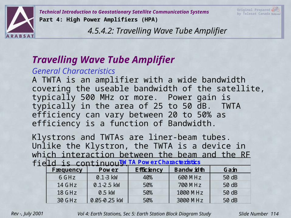
Technical Introduction to Geostationary Satellite Communication Systems Original Prepared by Telesat Canada
Slide Number 114Rev -, July 2001
Travelling Wave Tube AmplifierGeneral CharacteristicsA TWTA is an amplifier with a wide bandwidth covering the useable bandwidth of the satellite, typically 500 MHz or more. Power gain is typically in the area of 25 to 50 dB. TWTA efficiency can vary between 20 to 50% as efficiency is a function of Bandwidth.
Klystrons and TWTAs are liner-beam tubes. Unlike the Klystron, the TWTA is a device in which interaction between the beam and the RF field is continuous.
Frequency Power Efficiency Bandwidth Gain6 GHz 0.1-3 kW 40% 600 MHz 50 dB
14 GHz 0.1-2.5 kW 50% 700 MHz 50 dB18 GHz 0.5 kW 50% 1000 MHz 50 dB30 GHz 0.05-0.25 kW 50% 3000 MHz 50 dB
TWTA Power Characteristics
Part 4: High Power Amplifiers (HPA)
4.5.4.2: Travelling Wave Tube Amplifier
Vol 4: Earth Stations, Sec 5: Earth Station Block Diagram Study
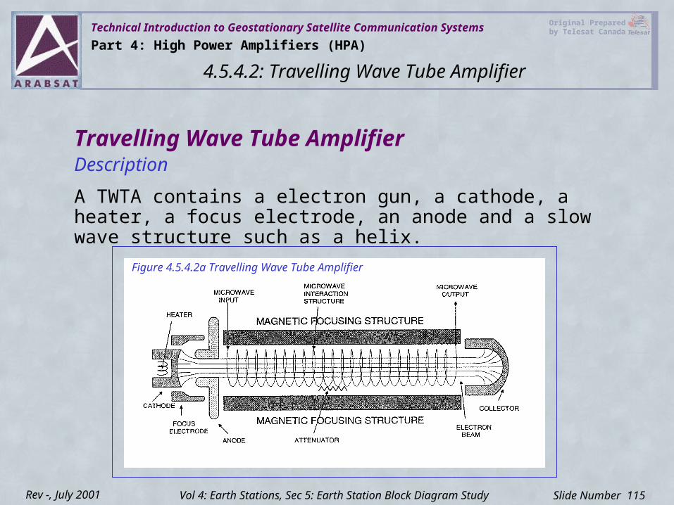
Technical Introduction to Geostationary Satellite Communication Systems Original Prepared by Telesat Canada
Slide Number 115Rev -, July 2001
Travelling Wave Tube AmplifierDescription
A TWTA contains a electron gun, a cathode, a heater, a focus electrode, an anode and a slow wave structure such as a helix.
Figure 4.5.4.2a Travelling Wave Tube Amplifier
Part 4: High Power Amplifiers (HPA)
4.5.4.2: Travelling Wave Tube Amplifier
Vol 4: Earth Stations, Sec 5: Earth Station Block Diagram Study
Technical Introduction to Geostationary Satellite Communication Systems Original Prepared by Telesat Canada
Slide Number 116Rev -, July 2001
Travelling Wave Tube AmplifierFundamentalsIn order to prolong the interaction between the electron beam and an RF field, it is necessary to ensure that both are moving in the same direction at approximately the same velocity.
This is quite different from the multicavity Klystron, in which the electron beam travels but the the RF field is stationary. The problem that must be solved is that an RF field travels with the velocity of light, while the electron beam’s velocity is unlikely to exceed 10% of that, even with a very high Anode voltage. The solution to this problem is to retard the RF field with a slow wave structure such as a helix and waveguide coupled cavity. This arrangement is the most common to TWTAs.
Part 4: High Power Amplifiers (HPA)
4.5.4.2: Travelling Wave Tube Amplifier
Vol 4: Earth Stations, Sec 5: Earth Station Block Diagram Study
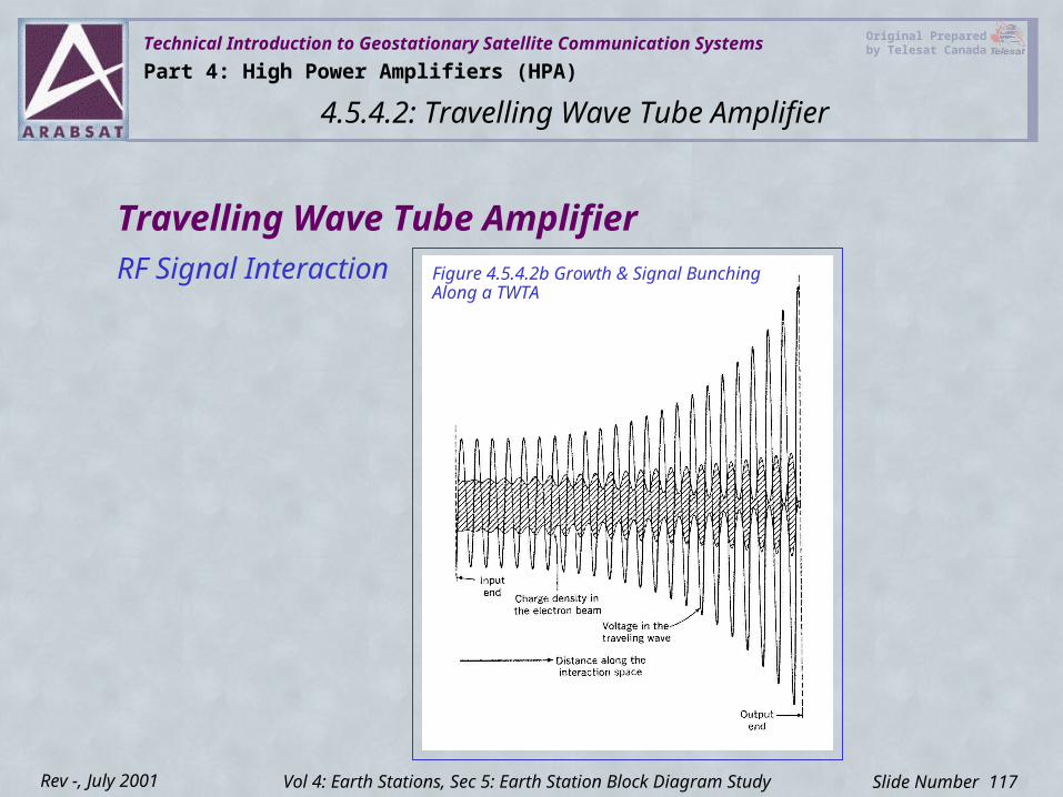
Technical Introduction to Geostationary Satellite Communication Systems Original Prepared by Telesat Canada
Slide Number 117Rev -, July 2001
Travelling Wave Tube AmplifierFigure 4.5.4.2b Growth & Signal Bunching Along a TWTA
RF Signal Interaction
Part 4: High Power Amplifiers (HPA)
4.5.4.2: Travelling Wave Tube Amplifier
Vol 4: Earth Stations, Sec 5: Earth Station Block Diagram Study
Technical Introduction to Geostationary Satellite Communication Systems Original Prepared by Telesat Canada
Slide Number 118Rev -, July 2001
Travelling Wave Tube AmplifierPrevention of OscillationsFigure 4.5.4.2b shows the exponential growth of oscillations along a TWTA. This growth is not to scale, as the actual gain could easily exceed 80 dB.
Oscillations are thus possible in a very high gain device, especially if poor load matching is created which causes significant reflections within the slow wave structure. The close coupling of the slow wave circuits can aggravate the problem as well.
To prevent these oscillations, all tubes use some form of attenuation to prevent this feedback from occurring. Both forward and reverse waves are attenuated but the forward wave is able to continue and grow past the attenuator. Overall gain of the tube is affected by adding this attenuation.
Part 4: High Power Amplifiers (HPA)
4.5.4.2: Travelling Wave Tube Amplifier
Vol 4: Earth Stations, Sec 5: Earth Station Block Diagram Study
Technical Introduction to Geostationary Satellite Communication Systems Original Prepared by Telesat Canada
Slide Number 119Rev -, July 2001
Travelling Wave Tube AmplifierFocusingThe electron beam is confined to a diameter that is smaller than the inside diameter of the slow wave structure. This is usually accomplished by providing a magnetic field in parallel with the direction of electron flow.
A large electromagnetic solenoid or a large permanent magnet can produce a magnetic field to keep the beam focused. However, to reduce bulk, periodic permanent magnet focusing is often used in TWTAs.
Periodic permanent magnet focusing employs a series of small magnets located along the length of the tube, with spaces between adjoining magnets. The beam defocuses slightly past each pole piece, but is refocused by the next magnet (note that individual magnets are interconnected).
Part 4: High Power Amplifiers (HPA)
4.5.4.2: Travelling Wave Tube Amplifier
Vol 4: Earth Stations, Sec 5: Earth Station Block Diagram Study
Technical Introduction to Geostationary Satellite Communication Systems Original Prepared by Telesat Canada
Slide Number 120Rev -, July 2001
Travelling Wave Tube AmplifierProper OPBO & DistortionsIn order to operate within the linear portion of the transfer curve, a TWTA can be operated at 3 dB OPBO or greater in single carrier mode. For multicarrier mode a TWTA must operate at 7 dB OPBO. The 3rd order IM spec of -26dB is the maximum IM level permitted in multicarrier mode. Typically, at this IM level, the OPBO is 7 dB.
AM/PM conversion in a TWTA is caused by the reduction in beam velocity that occurs as the input level signal is increased and greater amounts of energy are taken from the beam and transferred to the RF wave.
At 20 dB below the input required to saturate the TWT, AM/PM conversion is negligible. As the input is increased beyond this point, AM/PM conversion increases sharply.
Part 4: High Power Amplifiers (HPA)
4.5.4.2: Travelling Wave Tube Amplifier
Vol 4: Earth Stations, Sec 5: Earth Station Block Diagram Study
Technical Introduction to Geostationary Satellite Communication Systems Original Prepared by Telesat Canada
Slide Number 121Rev -, July 2001
Travelling Wave Tube AmplifierDistortions that occur to Klystrons also apply to TWTAs. Please refer to the Distortions area in the Klystron section.
LinearizersA linearizer is used to improve the intermodulation distortion (IMD) at its final output power caused by gain compression when an amplifier is operated near its saturation level.
A linearizer allows an amplifier to produce more output power and operate at a higher level of efficiency for a given level of distortion.
With Linearization, a TWTA may now be operated at 3 dB OPBO in multicarrier mode for FDMA, or with Digital Modulation only a 4 dB backoff may be required.
Part 4: High Power Amplifiers (HPA)
4.5.4.2: Travelling Wave Tube Amplifier
Vol 4: Earth Stations, Sec 5: Earth Station Block Diagram Study
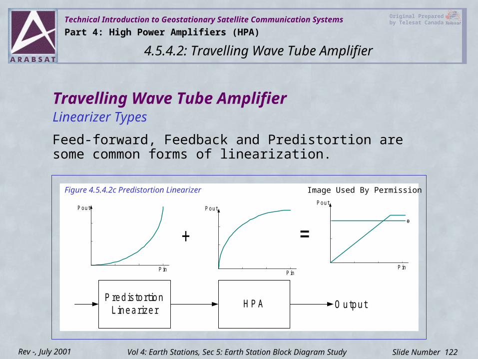
Technical Introduction to Geostationary Satellite Communication Systems Original Prepared by Telesat Canada
Slide Number 122Rev -, July 2001
Travelling Wave Tube AmplifierLinearizer Types
Feed-forward, Feedback and Predistortion are some common forms of linearization.
Pin
Pout
HPAPredistortionLinearizer Output
Pin
Pout
P in
Pout
+ =
Figure 4.5.4.2c Predistortion Linearizer
Part 4: High Power Amplifiers (HPA)
4.5.4.2: Travelling Wave Tube Amplifier
Vol 4: Earth Stations, Sec 5: Earth Station Block Diagram Study
Image Used By Permission
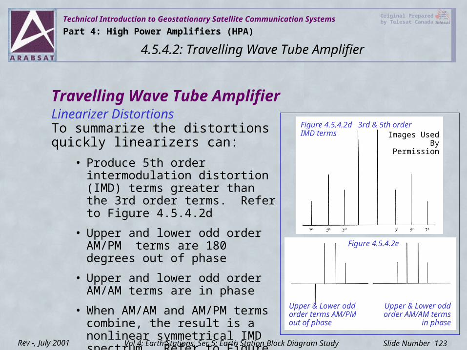
Technical Introduction to Geostationary Satellite Communication Systems Original Prepared by Telesat Canada
Slide Number 123Rev -, July 2001
Travelling Wave Tube AmplifierLinearizer DistortionsTo summarize the distortions quickly linearizers can:
• Produce 5th order intermodulation distortion (IMD) terms greater than the 3rd order terms. Refer to Figure 4.5.4.2d
• Upper and lower odd order AM/PM terms are 180 degrees out of phase
• Upper and lower odd order AM/AM terms are in phase
• When AM/AM and AM/PM terms combine, the result is a nonlinear symmetrical IMD spectrum. Refer to Figure 4.5.4.2e
Figure 4.5.4.2d 3rd & 5th order IMD terms
Upper & Lower odd order terms AM/PM out of phase
Upper & Lower odd order AM/AM terms
in phase
Figure 4.5.4.2e
Part 4: High Power Amplifiers (HPA)
4.5.4.2: Travelling Wave Tube Amplifier
Vol 4: Earth Stations, Sec 5: Earth Station Block Diagram Study
Images Used By Permission
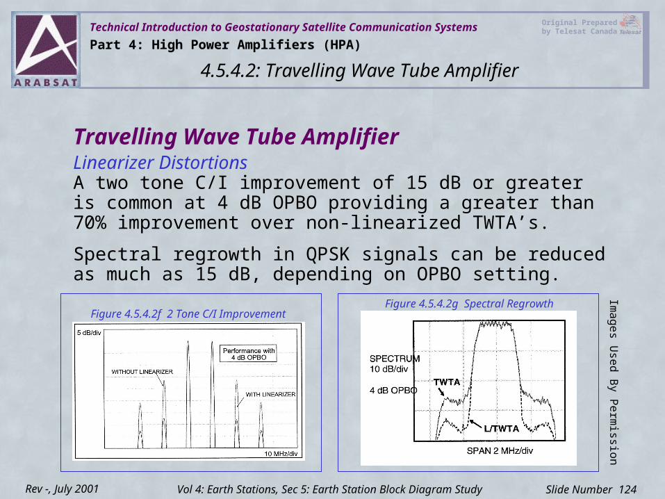
Technical Introduction to Geostationary Satellite Communication Systems Original Prepared by Telesat Canada
Slide Number 124Rev -, July 2001
Travelling Wave Tube AmplifierLinearizer DistortionsA two tone C/I improvement of 15 dB or greater is common at 4 dB OPBO providing a greater than 70% improvement over non-linearized TWTA’s.
Spectral regrowth in QPSK signals can be reduced as much as 15 dB, depending on OPBO setting.
Figure 4.5.4.2f 2 Tone C/I ImprovementFigure 4.5.4.2g Spectral Regrowth
Part 4: High Power Amplifiers (HPA)
4.5.4.2: Travelling Wave Tube Amplifier
Vol 4: Earth Stations, Sec 5: Earth Station Block Diagram Study
Images Used By Perm
ission
Technical Introduction to Geostationary Satellite Communication Systems Original Prepared by Telesat Canada
Slide Number 125Rev -, July 2001
Solid State Power AmplifierGeneral Characteristics Advances in field effect transistor (FET) and GaAsFET technology have significantly impacted satellite communications in spacecraft and Earth Station applications.
SSPAs have replaced TWTs in many Earth Station applications and some satellites are now all solid state as well.
SSPAs are a wideband device and will amplify the full spectrum of the satellite.
They require less power to operate and do not have high voltage power supplies like TWTs and Klystrons.
Part 4: High Power Amplifiers (HPA)
4.5.4.3: Solid State Power Amplifier
Vol 4: Earth Stations, Sec 5: Earth Station Block Diagram Study
Technical Introduction to Geostationary Satellite Communication Systems Original Prepared by Telesat Canada
Slide Number 126Rev -, July 2001
Solid State Power AmplifierSSPA Advantages
SSPA advantages over TWTAs are as follows:• Superior IMD performance
• High reliability
• Lower maintenance costs
• Lower spares costs
• Longer operating life compares to a TWTA (one SSPA can outlast several tubes)
• Higher personal safety as no high voltage power supplies are required
• Lower power consumption
• Lower cost of ownership
Part 4: High Power Amplifiers (HPA)
4.5.4.3: Solid State Power Amplifier
Vol 4: Earth Stations, Sec 5: Earth Station Block Diagram Study
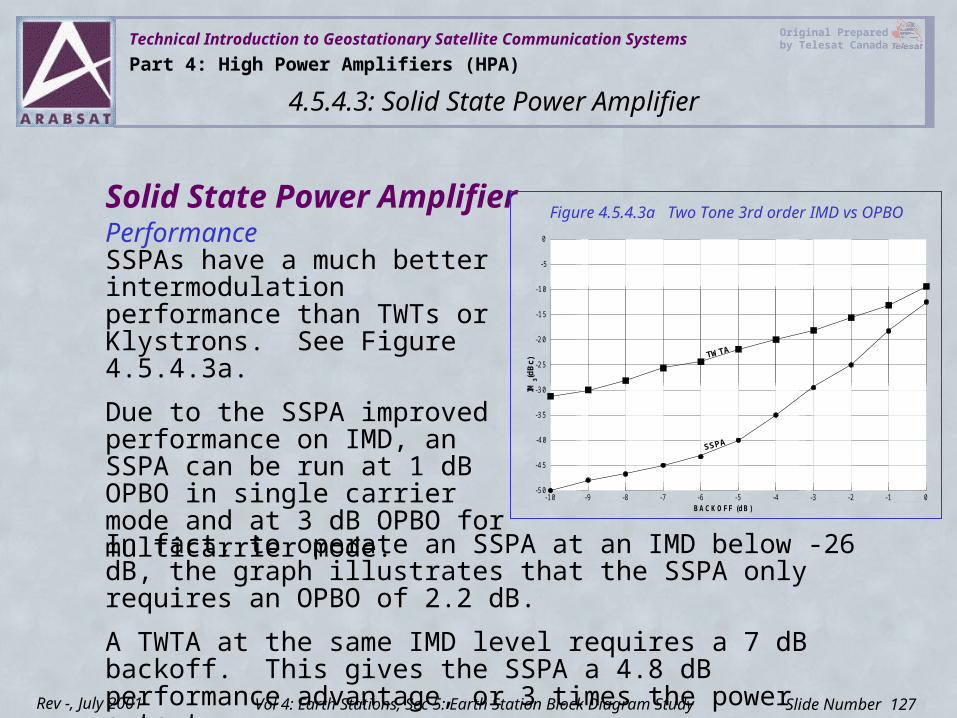
Technical Introduction to Geostationary Satellite Communication Systems Original Prepared by Telesat Canada
Slide Number 127Rev -, July 2001
Solid State Power AmplifierPerformanceSSPAs have a much better intermodulation performance than TWTs or Klystrons. See Figure 4.5.4.3a.
Due to the SSPA improved performance on IMD, an SSPA can be run at 1 dB OPBO in single carrier mode and at 3 dB OPBO for multicarrier mode.
Figure 4.5.4.3a Two Tone 3rd order IMD vs OPBO
In fact, to operate an SSPA at an IMD below -26 dB, the graph illustrates that the SSPA only requires an OPBO of 2.2 dB.
A TWTA at the same IMD level requires a 7 dB backoff. This gives the SSPA a 4.8 dB performance advantage, or 3 times the power output.
Part 4: High Power Amplifiers (HPA)
4.5.4.3: Solid State Power Amplifier
Vol 4: Earth Stations, Sec 5: Earth Station Block Diagram Study
-50
-40
-45
-35
-30
-25
-20
-15
-10
-5
0
-10 -9 -8 -7 -6 -5 -4 -3 -2 -1 0BACKOFF (dB)
IM (
dBc)
3
TWTA
SSPA
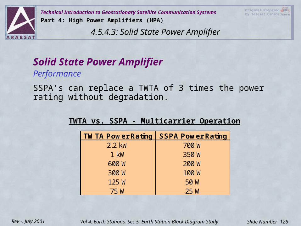
Technical Introduction to Geostationary Satellite Communication Systems Original Prepared by Telesat Canada
Slide Number 128Rev -, July 2001
Solid State Power AmplifierPerformance
SSPA’s can replace a TWTA of 3 times the power rating without degradation.
Part 4: High Power Amplifiers (HPA)
4.5.4.3: Solid State Power Amplifier
Vol 4: Earth Stations, Sec 5: Earth Station Block Diagram Study
TWTA Power Rating SSPA Power Rating2.2 kW 700 W1 kW 350 W
600 W 200 W300 W 100 W125 W 50 W75 W 25 W
TWTA vs. SSPA - Multicarrier Operation
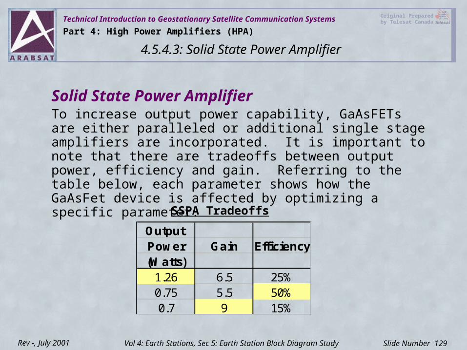
Technical Introduction to Geostationary Satellite Communication Systems Original Prepared by Telesat Canada
Slide Number 129Rev -, July 2001
Solid State Power AmplifierTo increase output power capability, GaAsFETs are either paralleled or additional single stage amplifiers are incorporated. It is important to note that there are tradeoffs between output power, efficiency and gain. Referring to the table below, each parameter shows how the GaAsFet device is affected by optimizing a specific parameter.
Output Power Gain Efficiency(Watts)
1.26 6.5 25%0.75 5.5 50%0.7 9 15%
SSPA Tradeoffs
Part 4: High Power Amplifiers (HPA)
4.5.4.3: Solid State Power Amplifier
Vol 4: Earth Stations, Sec 5: Earth Station Block Diagram Study
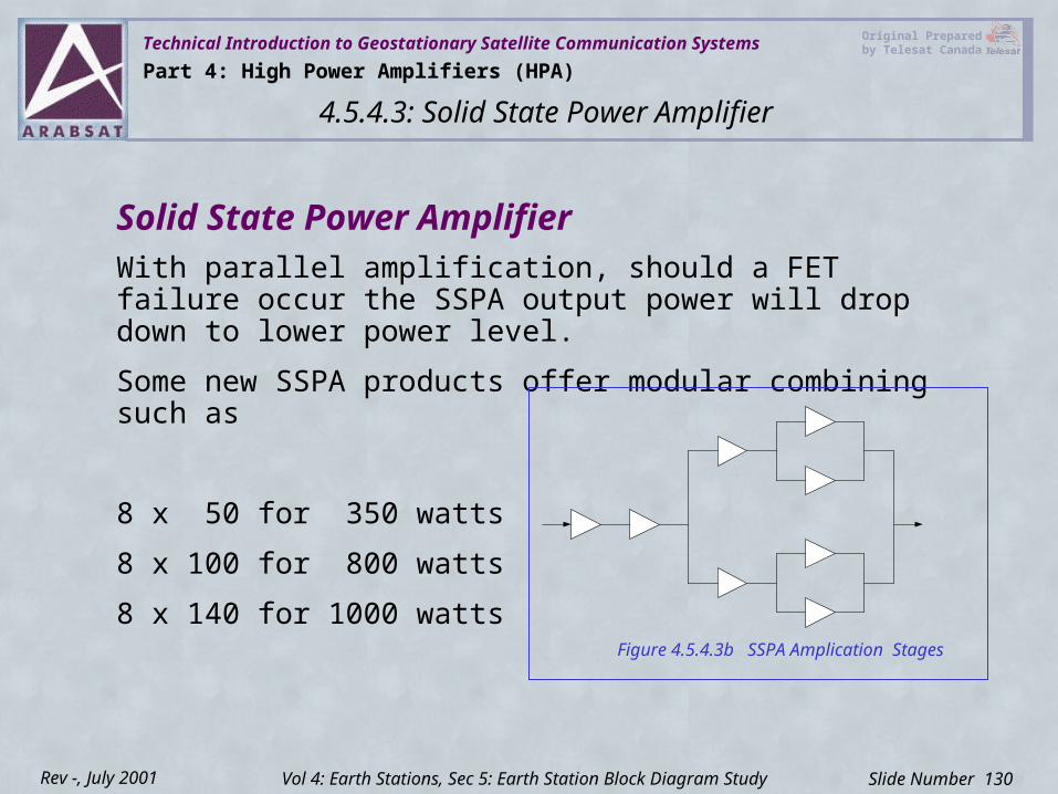
Technical Introduction to Geostationary Satellite Communication Systems Original Prepared by Telesat Canada
Slide Number 130Rev -, July 2001
With parallel amplification, should a FET failure occur the SSPA output power will drop down to lower power level.
Some new SSPA products offer modular combining such as
8 x 50 for 350 watts
8 x 100 for 800 watts
8 x 140 for 1000 watts
Figure 4.5.4.3b SSPA Amplication Stages
Solid State Power Amplifier
Part 4: High Power Amplifiers (HPA)
4.5.4.3: Solid State Power Amplifier
Vol 4: Earth Stations, Sec 5: Earth Station Block Diagram Study
Technical Introduction to Geostationary Satellite Communication Systems Original Prepared by Telesat Canada
Slide Number 131Rev -, July 2001
Comparison of all three typesWhen is a Klystron used over a TWTA?A Klyston is used when high power is required, as they have historically always provided higher power than TWTAs. Disadvantages: high cost, narrow band, tuner may be required.
When is a TWTA used over a SSPA (assuming linearity & IMD characteristics are similar)? Advantage: both are wideband devices.
• A rule of thumb: if 400 watts or higher is required (C-Band), A TWTA would be chosen over a SSPA. Below 400 watts an SSPA would be chosen as they are more cost effective.
• Below 300 watts a SSPA will consume less prime power (AC).
• Reliability of TWTAs has improved, and a study by Intelsat on their satellites has shown that the failure rate of TWTAs is 15% better than SSPAs.
Part 4: High Power Amplifiers (HPA)
4.5.4.4: Comparison of All Three Types
Vol 4: Earth Stations, Sec 5: Earth Station Block Diagram Study
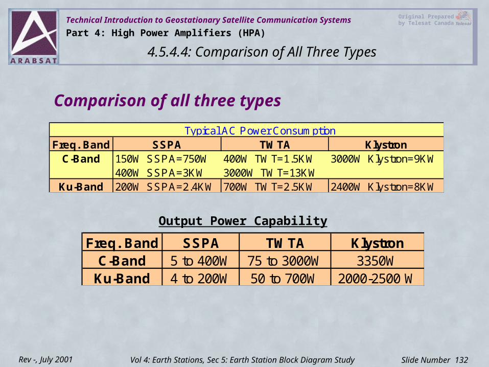
Technical Introduction to Geostationary Satellite Communication Systems Original Prepared by Telesat Canada
Slide Number 132Rev -, July 2001
Freq. Band SSPA TWTA KlystronC-Band 5 to 400W 75 to 3000W 3350W
Ku-Band 4 to 200W 50 to 700W 2000-2500 W
Output Power Capability
Freq. Band SSPA TWTA KlystronC-Band 150W SSPA=750W 400W TWT=1.5KW 3000W Klystron=9KW
400W SSPA=3KW 3000W TWT=13KWKu-Band 200W SSPA=2.4KW 700W TWT=2.5KW 2400W Klystron=8KW
Typical AC Power Consumption
Comparison of all three types
Part 4: High Power Amplifiers (HPA)
4.5.4.4: Comparison of All Three Types
Vol 4: Earth Stations, Sec 5: Earth Station Block Diagram Study
Technical Introduction to Geostationary Satellite Communication Systems Original Prepared by Telesat Canada
Slide Number 133Rev -, July 2001
Comparison of all Three TypesA combination of factors must be considered when choosing between types of amplifiers such as
• Cost
• Specifications - gain, linearity, IMD
• Temperature capability
• Indoor or outdoor mounted
• Reliability
• Power consumption
• HVAC requirements
• Size limitations and redundancy requirement
Only when you have gathered a significant combination of the above information can a informed decision be made.
Part 4: High Power Amplifiers (HPA)
4.5.4.4: Comparison of All Three Types
Vol 4: Earth Stations, Sec 5: Earth Station Block Diagram Study
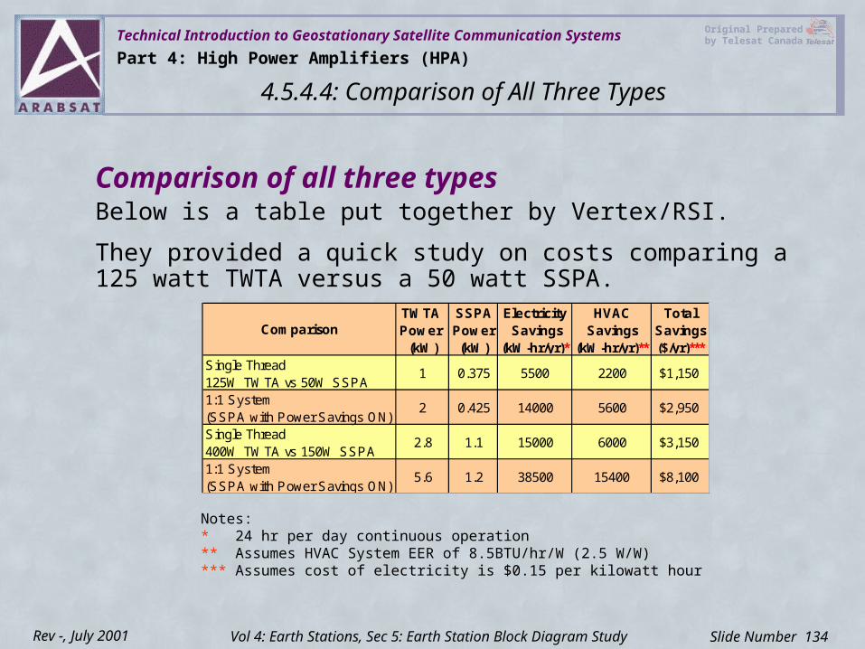
Technical Introduction to Geostationary Satellite Communication Systems Original Prepared by Telesat Canada
Slide Number 134Rev -, July 2001
Comparison of all three typesBelow is a table put together by Vertex/RSI.
They provided a quick study on costs comparing a 125 watt TWTA versus a 50 watt SSPA.
TWTA SSPA Electricity HVAC TotalPower Power Savings Savings Savings
(kW) (kW) (kW-hr/yr)* (kW-hr/yr)** ($/yr)***Single Thread125W TWTA vs 50W SSPA1:1 System(SSPA with Power Savings ON)Single Thread400W TWTA vs 150W SSPA1:1 System(SSPA with Power Savings ON)
2200
6000
$1,150
2 0.425 14000 5600 $2,950
1 0.375 5500
Comparison
$3,150
5.6 1.2 38500 15400 $8,100
2.8 1.1 15000
Notes:* 24 hr per day continuous operation** Assumes HVAC System EER of 8.5BTU/hr/W (2.5 W/W)*** Assumes cost of electricity is $0.15 per kilowatt hour
Part 4: High Power Amplifiers (HPA)
4.5.4.4: Comparison of All Three Types
Vol 4: Earth Stations, Sec 5: Earth Station Block Diagram Study
Technical Introduction to Geostationary Satellite Communication Systems Original Prepared by Telesat Canada
Slide Number 135Rev -, July 2001
Up and Down ConversionPart 5
Vol 4: Earth Stations
4.5: Earth Station Block Diagram Study
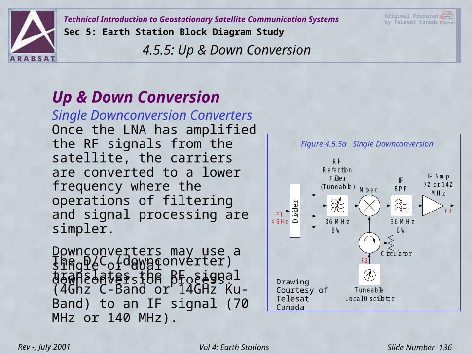
Technical Introduction to Geostationary Satellite Communication Systems Original Prepared by Telesat Canada
Slide Number 136Rev -, July 2001
Up & Down ConversionSingle Downconversion ConvertersOnce the LNA has amplified the RF signals from the satellite, the carriers are converted to a lower frequency where the operations of filtering and signal processing are simpler.
Downconverters may use a single or dual downconversion process.
Figure 4.5.5a Single Downconversion
The D/C (downconverter) translates the RF signal (4Ghz C-Band or 14GHz Ku-Band) to an IF signal (70 MHz or 140 MHz).
IFB P F
36 M H zB W
M ixer
T uneab leLocal O scilla to r
C ircu la tor
RFRefection
F ilte r(Tuneab le)
IF Am p70 or 140
M Hz
36 M HzB W
F14 G H z D
ivid
er
F2
F3
Drawing Courtesy of Telesat Canada
Sec 5: Earth Station Block Diagram Study
4.5.5: Up & Down Conversion
Vol 4: Earth Stations
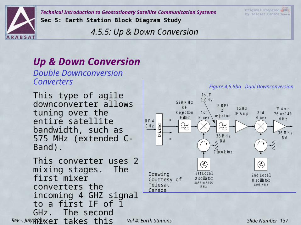
Technical Introduction to Geostationary Satellite Communication Systems Original Prepared by Telesat Canada
Slide Number 137Rev -, July 2001
Up & Down ConversionDouble Downconversion Converters
This type of agile downconverter allows tuning over the entire satellite bandwidth, such as 575 MHz (extended C-Band).
This converter uses 2 mixing stages. The first mixer converters the incoming 4 GHZ signal to a first IF of 1 GHz. The second mixer takes this signal and converts it to a 70 or 140 MHz second IF frequency.
Figure 4.5.5ba Dual Downconversion
IF BPF&
re jection
36 M HzBW
1stM ixer
1st Loca lO scilla to r48 55 to 53 55
M H z
Circulator
1G H zIF A m p
RF 4G H z
Div
ider
1s t IF1 G H z
36 M HzBW
500 M HzR F
R ejectionFilte r
IF A m p70 o r 140
M Hz2nd
M ixer
2nd Loca lO scilla tor
12 95 M H z
Drawing Courtesy of Telesat Canada
Sec 5: Earth Station Block Diagram Study
4.5.5: Up & Down Conversion
Vol 4: Earth Stations
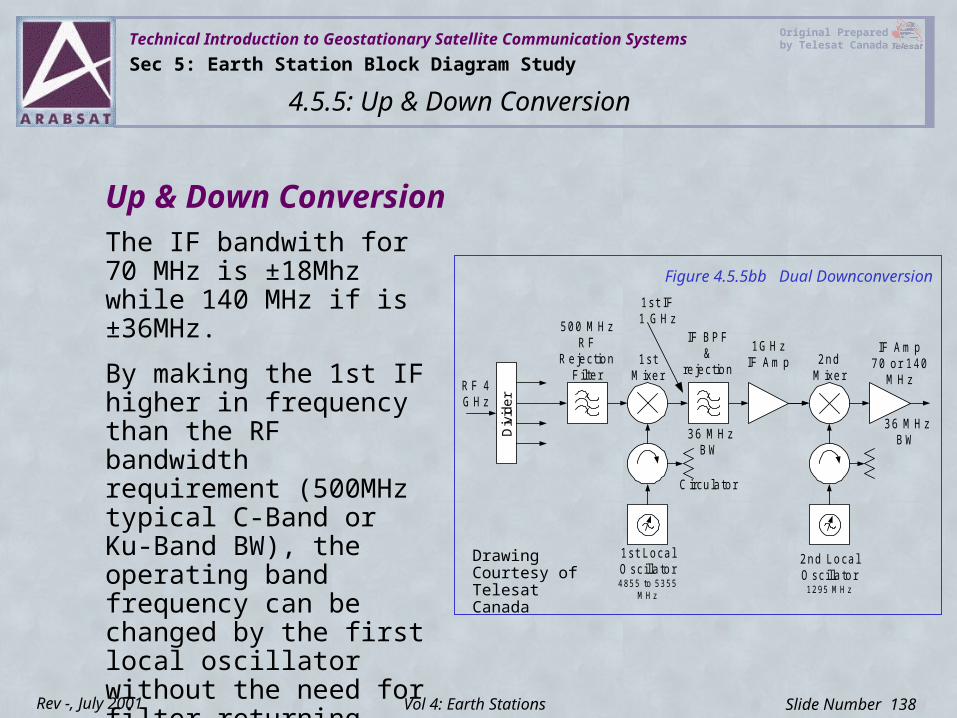
Technical Introduction to Geostationary Satellite Communication Systems Original Prepared by Telesat Canada
Slide Number 138Rev -, July 2001
The IF bandwith for 70 MHz is ±18Mhz while 140 MHz if is ±36MHz.
By making the 1st IF higher in frequency than the RF bandwidth requirement (500MHz typical C-Band or Ku-Band BW), the operating band frequency can be changed by the first local oscillator without the need for filter returning.
Up & Down Conversion
Figure 4.5.5bb Dual Downconversion
IF BPF&
re jection
36 M HzBW
1stM ixer
1st Loca lO scilla to r48 55 to 53 55
M H z
Circulator
1G H zIF A m p
RF 4G H z
Div
ider
1s t IF1 G H z
36 M HzBW
500 M HzR F
R ejectionFilte r
IF A m p70 o r 140
M Hz2nd
M ixer
2nd Loca lO scilla tor
12 95 M H z
Drawing Courtesy of Telesat Canada
Sec 5: Earth Station Block Diagram Study
4.5.5: Up & Down Conversion
Vol 4: Earth Stations
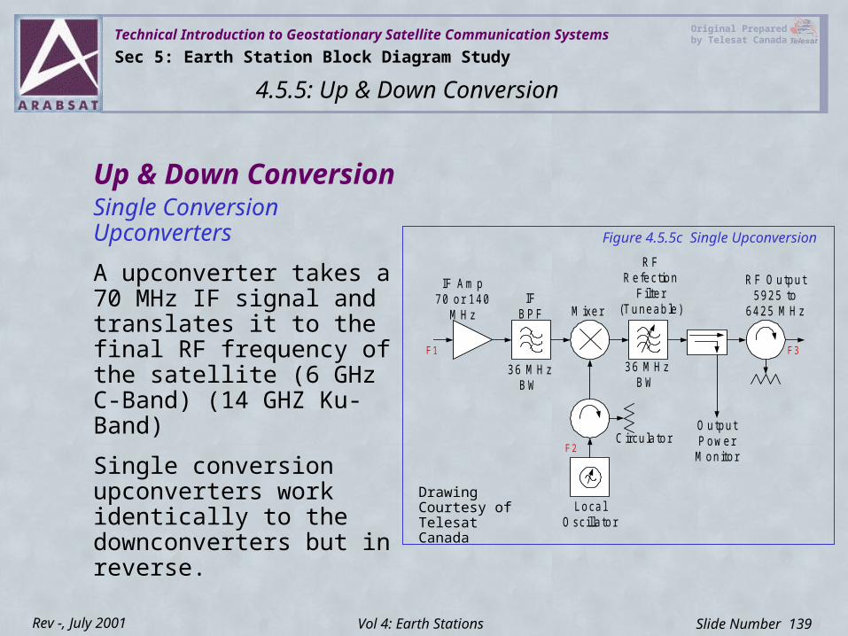
Technical Introduction to Geostationary Satellite Communication Systems Original Prepared by Telesat Canada
Slide Number 139Rev -, July 2001
Up & Down ConversionSingle Conversion Upconverters
A upconverter takes a 70 MHz IF signal and translates it to the final RF frequency of the satellite (6 GHz C-Band) (14 GHZ Ku-Band)
Single conversion upconverters work identically to the downconverters but in reverse.
IF A m p70 or 140
M H zIF
B PF
36 M H zB W
M ixer
LocalO scilla to r
C ircu lator
R FR efection
F ilte r(T uneab le)
O utputPower
M onitor
R F O utput5925 to
6425 M H z
36 M H zBW
F1
F2
F3
Figure 4.5.5c Single Upconversion
Drawing Courtesy of Telesat Canada
Sec 5: Earth Station Block Diagram Study
4.5.5: Up & Down Conversion
Vol 4: Earth Stations
Technical Introduction to Geostationary Satellite Communication Systems Original Prepared by Telesat Canada
Slide Number 140Rev -, July 2001
Example:
F1 - 70 MHz IF
F2 - 5930 MHz mixing freq. (LO)
F3 - 6000 GHz wanted output freq.
By mixing F1 & F2 the mixer produces
5930 MHz+70 MHz = 6000 MHz
5930 MHz -70 MHz = 5860 MHz
The bandpass filter, filters out the unwanted sideband of 5860 MHz.
Up & Down Conversion
Sec 5: Earth Station Block Diagram Study
4.5.5: Up & Down Conversion
Vol 4: Earth Stations
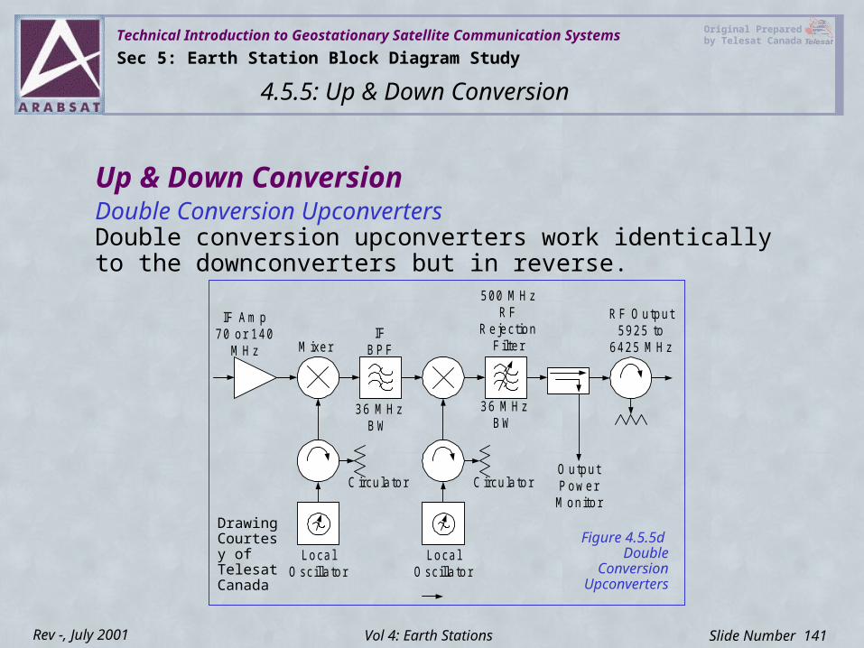
Technical Introduction to Geostationary Satellite Communication Systems Original Prepared by Telesat Canada
Slide Number 141Rev -, July 2001
Up & Down ConversionDouble Conversion Upconverters Double conversion upconverters work identically to the downconverters but in reverse.
IF A m p70 o r 140
M H z M ixer
Loca lO scilla to r
C ircu la tor
500 M H zR F
R ejectionF ilte r
36 M H zBW
IFB PF
36 M H zBW
LocalO scilla tor
C ircu la torO utputP ow er
M onitor
R F O utpu t5925 to
6425 M H z
Figure 4.5.5d Double
Conversion Upconverters
Drawing Courtesy of Telesat Canada
Sec 5: Earth Station Block Diagram Study
4.5.5: Up & Down Conversion
Vol 4: Earth Stations
Technical Introduction to Geostationary Satellite Communication Systems Original Prepared by Telesat Canada
Slide Number 142Rev -, July 2001
Up & Down ConversionOscillatorsThe local oscillators inside frequency converters can be crystal controlled devices or frequency synthesizers. These oscillators are critical to the operation of the converter and must be stable enough for the specific application.
Typical important specifications are frequency stability short term and long term, rated in ppm (parts per million), temperature stability in ppm over a specified temperature, and phase noise.
Sec 5: Earth Station Block Diagram Study
4.5.5: Up & Down Conversion
Vol 4: Earth Stations
Technical Introduction to Geostationary Satellite Communication Systems Original Prepared by Telesat Canada
Slide Number 143Rev -, July 2001
Different types of oscillators are:
• XO Non-compensated crystal oscillators
• TCXO Temperature compensated crystal oscillators
• OCXO Oven controlled crystal oscillators
• VCXO Voltage controlled crystal oscillators
• Microprocessor Compensated
• Disciplined Oscillators
• Multi-Crystal Oscillators
Up & Down Conversion
Sec 5: Earth Station Block Diagram Study
4.5.5: Up & Down Conversion
Vol 4: Earth Stations
Technical Introduction to Geostationary Satellite Communication Systems Original Prepared by Telesat Canada
Slide Number 144Rev -, July 2001
Up & Down ConversionFrequency OffsetsFrequency offsets occur when the oscillator frequency is not set exactly to the desired frequency. This can result from frequency drift due to long term variations (aging) or short term random frequency variations, such as might be caused by vibration or temperature changes.
A 5 MHz oscillator having a stability of ±2 ppm would be expected to produce a output frequency that is ±10Hz of the desired 5 MHz output. Example : If the 5 MHz oscillator was 1 Hz high and a 6 GHz output frequency was required at the final output this would translate to a 1200 Hz frequency offset.
Therefore it becomes very important to have an accurate and properly specified up and downconverter for the desired service.
Sec 5: Earth Station Block Diagram Study
4.5.5: Up & Down Conversion
Vol 4: Earth Stations
Technical Introduction to Geostationary Satellite Communication Systems Original Prepared by Telesat Canada
Slide Number 145Rev -, July 2001
Up & Down ConversionExternal Frequency ReferenceExternal Frequency Reference allows the converter to be frequency-locked to GPS. An external 5 MHz or 10 MHz clock input phase locks the converter so output frequencies become very accurate.
This provides the advantage of locking all uplink and downlink sites so very little frequency offset occurs.
GPS receivers offer accuracies typically <1x10-12 when tracking satellites.
Sec 5: Earth Station Block Diagram Study
4.5.5: Up & Down Conversion
Vol 4: Earth Stations
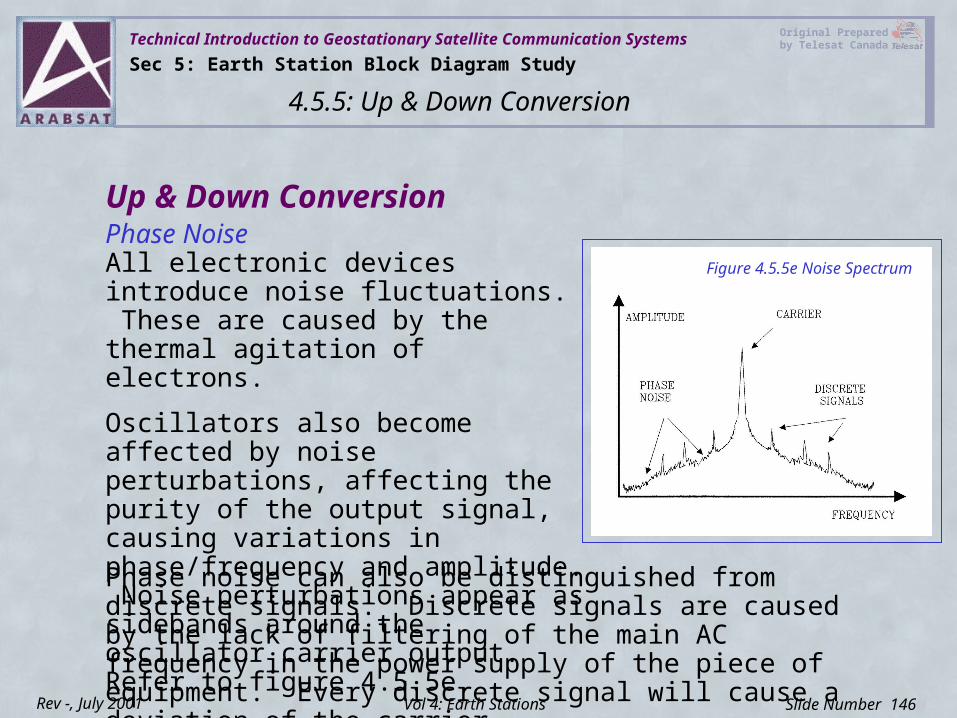
Technical Introduction to Geostationary Satellite Communication Systems Original Prepared by Telesat Canada
Slide Number 146Rev -, July 2001
Up & Down ConversionPhase NoiseAll electronic devices introduce noise fluctuations. These are caused by the thermal agitation of electrons.
Oscillators also become affected by noise perturbations, affecting the purity of the output signal, causing variations in phase/frequency and amplitude. Noise perturbations appear as sidebands around the oscillator carrier output. Refer to figure 4.5.5e.
Figure 4.5.5e Noise Spectrum
Phase noise can also be distinguished from discrete signals. Discrete signals are caused by the lack of filtering of the main AC frequency in the power supply of the piece of equipment. Every discrete signal will cause a deviation of the carrier.
Sec 5: Earth Station Block Diagram Study
4.5.5: Up & Down Conversion
Vol 4: Earth Stations
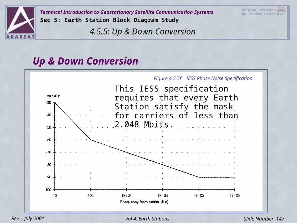
Technical Introduction to Geostationary Satellite Communication Systems Original Prepared by Telesat Canada
Slide Number 147Rev -, July 2001
Up & Down ConversionFigure 4.5.5f IESS Phase Noise Specification
Sec 5: Earth Station Block Diagram Study
4.5.5: Up & Down Conversion
Vol 4: Earth Stations
This IESS specification requires that every Earth Station satisfy the mask for carriers of less than 2.048 Mbits.
Technical Introduction to Geostationary Satellite Communication Systems Original Prepared by Telesat Canada
Slide Number 148Rev -, July 2001
Up & Down ConversionPhase Noise Problems
If phase noise specs were left unattended the largest problem experienced would be the degradation of BER performance of digital systems using any type of phase modulation (burst, trickle and steady errors).
Sec 5: Earth Station Block Diagram Study
4.5.5: Up & Down Conversion
Vol 4: Earth Stations
Technical Introduction to Geostationary Satellite Communication Systems Original Prepared by Telesat Canada
Slide Number 149Rev -, July 2001
ModemsPart 6
Vol 4: Earth Stations
4.5: Earth Station Block Diagram Study
Technical Introduction to Geostationary Satellite Communication Systems Original Prepared by Telesat Canada
Slide Number 150Rev -, July 2001
ModemsA modem is a modulator/demodulator which converts input/output information acquired via an interface to a intermediate frequency of 70MHz, 140MHz or L-Band.
The modulator processes the information—such as speech, music, pictures—and alters a carrier with the intelligence in one of three possible ways: by varying its amplitude (AM), by varying its frequency (FM), or by varying the phase of the carrier (PM).
The demodulator is used to extract the information from the modulated waveform using the reverse process originally performed in the modulator.
The modulator and demodulator can also be individual units, but are typically combined into one unit.
The output of the modulator/input to the demodulator is normally in the 70 MHz IF band (52 MHz to 88 MHz).
Sec 5: Earth Station Block Diagram Study
4.5.6: Modems
Vol 4: Earth Stations
Technical Introduction to Geostationary Satellite Communication Systems Original Prepared by Telesat Canada
Slide Number 151Rev -, July 2001
ModemsMost modems in satellite communications are data modems.
Dependant of the data speed and protocol, the data input connector could be an RS232, V.35, RS422, X.21, or ethernet type digital interface employing or RJ45, twisted pair terminal block, DB9, or DB25 or other configuration. Today's digital modems typically offer variable data rates from 2.4 to 2048 Kbps in BPSK, QPSK and sometimes 0PSK (Offset QPSK) and 8PSK modes. Specialty modems offer higher data rates and 16PSK.
Viterbi and sequential forward error correction are available, with Reed Solomon Codec for additional coding gains.
Recent development in FEC techniques involve Turbo coding that delivers significant performance improvement when compared to Viterbi concatenated with Reed-Solomon. Turbo coding offers increased coding gain, lower decoding delay, and bandwidth savings of up to 40%.
Sec 5: Earth Station Block Diagram Study
4.5.6: Modems
Vol 4: Earth Stations
Technical Introduction to Geostationary Satellite Communication Systems Original Prepared by Telesat Canada
Slide Number 152Rev -, July 2001
ExcitersPart 7
Vol 4: Earth Stations
4.5: Earth Station Block Diagram Study
Technical Introduction to Geostationary Satellite Communication Systems Original Prepared by Telesat Canada
Slide Number 153Rev -, July 2001
ExcitersA video exciter converts a baseband analog video and audio signal to an RF output at 6 or 14 GHz.
A video exciter is typically composed of:• Video baseband processor
• Audio subcarrier modulator
• Wideband modulator
• IF amplifier and filter
• Upconverter
Most exciters are modular, with removable plug-in modules for fast easy repair. Some modules are equipped with LEDs for status indication and controls for adjustment.
Sec 5: Earth Station Block Diagram Study
4.5.7: Exciters
Vol 4: Earth Stations
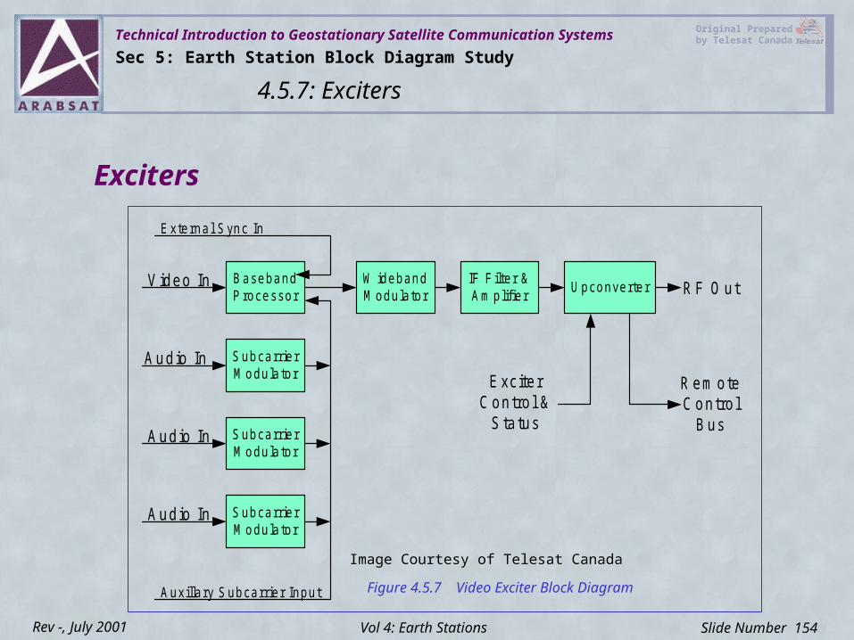
Technical Introduction to Geostationary Satellite Communication Systems Original Prepared by Telesat Canada
Slide Number 154Rev -, July 2001
BasebandProcessor
SubcarrierM odulato r
SubcarrierM odulato r
SubcarrierM odulato r
W idebandM odulator
IF F ilte r &Am plifier U pconverter R F O ut
R em oteC ontro l
B us
E xcite rC ontro l &
S ta tus
External Sync In
V ideo In
A udio In
A udio In
A udio In
Auxilla ry Subcarrie r Input Figure 4.5.7 Video Exciter Block Diagram
Exciters
Image Courtesy of Telesat Canada
Sec 5: Earth Station Block Diagram Study
4.5.7: Exciters
Vol 4: Earth Stations
Technical Introduction to Geostationary Satellite Communication Systems Original Prepared by Telesat Canada
Slide Number 155Rev -, July 2001
ExcitersVideo exciters are not as popular today as they were 10 years ago.
Analog video exciters are being replaced by modern DVC equipment for most new occasional use broadcast.
Video exciters are primarily used for occasional use video feeds.
Sec 5: Earth Station Block Diagram Study
4.5.7: Exciters
Vol 4: Earth Stations

Technical Introduction to Geostationary Satellite Communication Systems Original Prepared by Telesat Canada
Slide Number 156Rev -, July 2001
Baseband EquipmentPart 8
Vol 4: Earth Stations
4.5: Earth Station Block Diagram Study
Technical Introduction to Geostationary Satellite Communication Systems Original Prepared by Telesat Canada
Slide Number 157Rev -, July 2001
Contents
4.5.8.1 Multiplexers4.5.8.2 Digital Video Devices4.5.8.3 CSU/DSU’s4.5.8.4 Channel Banks4.5.8.5 Routers & Hubs4.5.8.6 PBX Equipment
Vol 4: Earth Stations
4.5: Earth Station Block Diagram Study
Technical Introduction to Geostationary Satellite Communication Systems Original Prepared by Telesat Canada
Slide Number 158Rev -, July 2001
MultiplexersA Multiplexer is a device that combines several low speed channels into one high speed channel.
A Mux can combine a variety of formats such as voice, data and video.
Voice signals are first converted to digital, and some Muxes will use compression to further reduce the bandwidth. A standard voice circuit once converted to digital becomes a PCM 64 Kbps circuit and can be compressed further to 32 Kbps (ADPCM), 16 Kbps (LD-CELP), 8 kbps (A-CELP) or less.
Voice interfaces can include, E&M, FXO, FXS, T1, E1.
Part 8: Baseband Equipment
4.5.8.1: Multiplexers
Vol 4: Earth Stations, Sec 5: Earth Station Block Diagram Study
Technical Introduction to Geostationary Satellite Communication Systems Original Prepared by Telesat Canada
Slide Number 159Rev -, July 2001
MultiplexersThe combined output of a multiplexer is called the “Aggregate”. Aggregate interfaces can include, T1, E1, Fractional, X.21, V.35, ISDN.
Packet services such as Frame Relay, VOIP, VOFR, HDLC, ATM, X.25 can also be offered.
Types of Multiplexing
1) Frequency Division Multiplexing
2) Time Division Multiplexing
3) Statistical Multiplexing
Part 8: Baseband Equipment
4.5.8.1: Multiplexers
Vol 4: Earth Stations, Sec 5: Earth Station Block Diagram Study
Technical Introduction to Geostationary Satellite Communication Systems Original Prepared by Telesat Canada
Slide Number 160Rev -, July 2001
MultiplexersFrequency Division Multiplexing FDM is an analog method of combining several communication channels over the same transmission facility at the same time.
In FDM, each channel uses a different band of frequencies so that there is no interference between channels.
FDM was the most commonly used by multiplexers in the early 1960’s for early telephone trunk and radio systems.
FDM had a upper limit of 13,200 voice circuits.
Part 8: Baseband Equipment
4.5.8.1: Multiplexers
Vol 4: Earth Stations, Sec 5: Earth Station Block Diagram Study
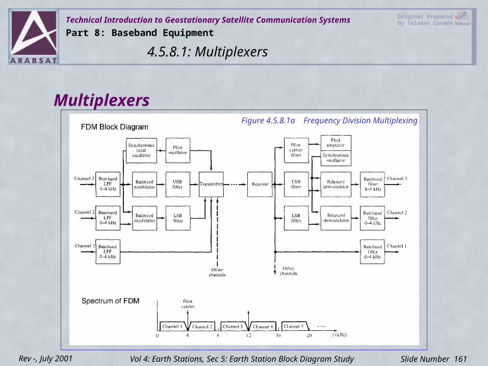
Technical Introduction to Geostationary Satellite Communication Systems Original Prepared by Telesat Canada
Slide Number 161Rev -, July 2001
Figure 4.5.8.1a Frequency Division Multiplexing
Multiplexers
Part 8: Baseband Equipment
4.5.8.1: Multiplexers
Vol 4: Earth Stations, Sec 5: Earth Station Block Diagram Study
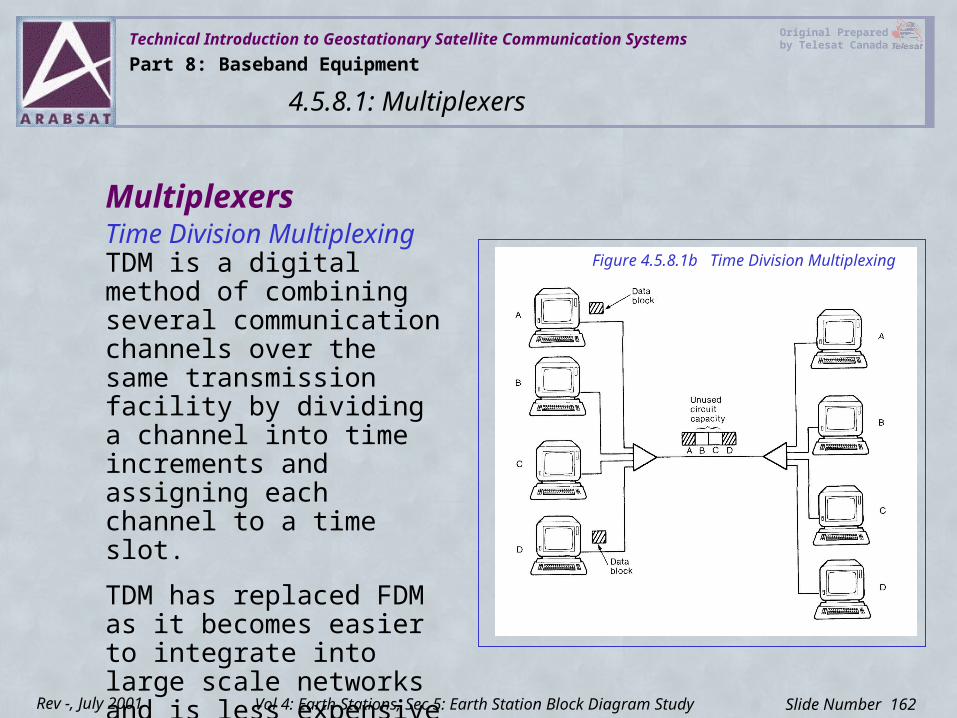
Technical Introduction to Geostationary Satellite Communication Systems Original Prepared by Telesat Canada
Slide Number 162Rev -, July 2001
MultiplexersTime Division Multiplexing TDM is a digital method of combining several communication channels over the same transmission facility by dividing a channel into time increments and assigning each channel to a time slot.
TDM has replaced FDM as it becomes easier to integrate into large scale networks and is less expensive to manufacture.
Figure 4.5.8.1b Time Division Multiplexing
Part 8: Baseband Equipment
4.5.8.1: Multiplexers
Vol 4: Earth Stations, Sec 5: Earth Station Block Diagram Study
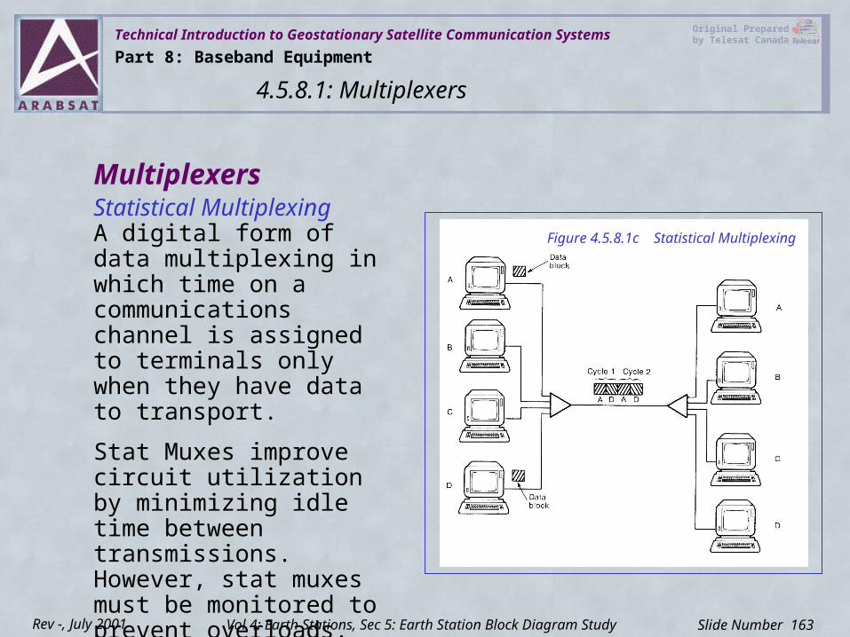
Technical Introduction to Geostationary Satellite Communication Systems Original Prepared by Telesat Canada
Slide Number 163Rev -, July 2001
MultiplexersStatistical MultiplexingA digital form of data multiplexing in which time on a communications channel is assigned to terminals only when they have data to transport.
Stat Muxes improve circuit utilization by minimizing idle time between transmissions. However, stat muxes must be monitored to prevent overloads.
Figure 4.5.8.1c Statistical Multiplexing
Part 8: Baseband Equipment
4.5.8.1: Multiplexers
Vol 4: Earth Stations, Sec 5: Earth Station Block Diagram Study
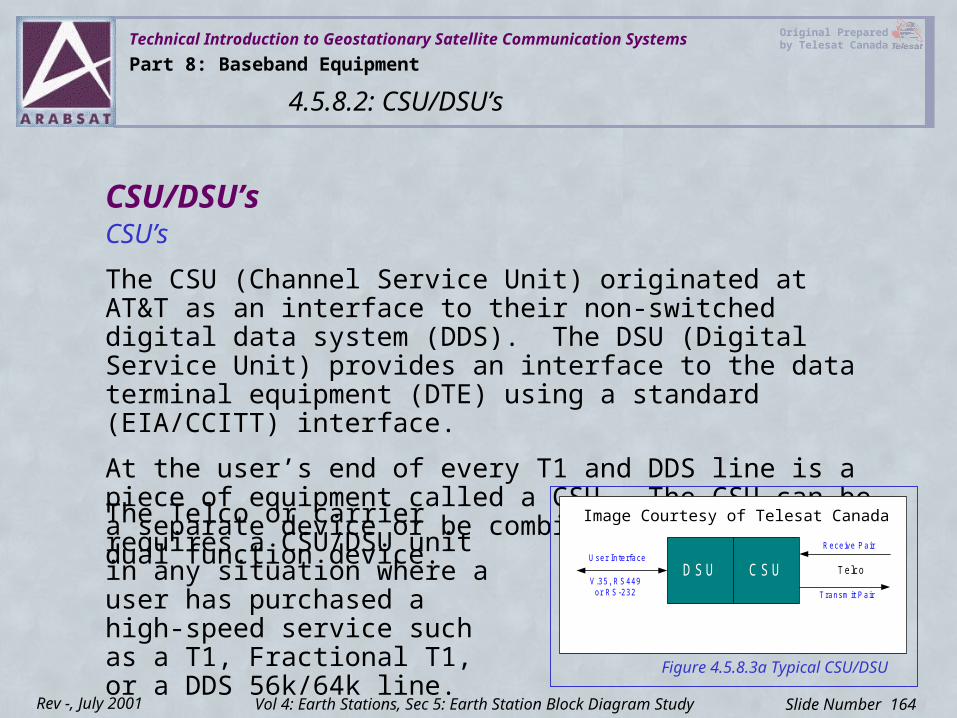
Technical Introduction to Geostationary Satellite Communication Systems Original Prepared by Telesat Canada
Slide Number 164Rev -, July 2001
CSU/DSU’sCSU’s
The CSU (Channel Service Unit) originated at AT&T as an interface to their non-switched digital data system (DDS). The DSU (Digital Service Unit) provides an interface to the data terminal equipment (DTE) using a standard (EIA/CCITT) interface.
At the user’s end of every T1 and DDS line is a piece of equipment called a CSU. The CSU can be a separate device or be combined with a DSU as a dual function device.
U ser In terface
V.35, R S449or R S-232
D SU
R ece ive Pair
T ransm it P air
TelcoCS U
Figure 4.5.8.3a Typical CSU/DSU
The Telco or carrier requires a CSU/DSU unit in any situation where a user has purchased a high-speed service such as a T1, Fractional T1, or a DDS 56k/64k line.
Image Courtesy of Telesat Canada
Part 8: Baseband Equipment
4.5.8.2: CSU/DSU’s
Vol 4: Earth Stations, Sec 5: Earth Station Block Diagram Study
Technical Introduction to Geostationary Satellite Communication Systems Original Prepared by Telesat Canada
Slide Number 165Rev -, July 2001
CSU/DSU’sMultiplexer CSU/DSUs
If the T1 CSU/DSU has more than one user port, it can function as a multiplexer allocating the DS-0 time slots between the ports in multiples of 64 kbps or 56 kbps.
For voice applications, a DSX, DS1 or optional T1 tail circuit is available.
The DSX Option:• Provides a tail circuit in
Telco format for connection to a PBX voice system
• Must be within 655 feet of the CSU/DSU
The DS1 Option: • Provides a tail circuit in Telco
format for connection to a PBX voice system
• Allows for greater distance from the CSU/DSU to the PBX—up to 6000 feet
Part 8: Baseband Equipment
4.5.8.2: CSU/DSU’s
Vol 4: Earth Stations, Sec 5: Earth Station Block Diagram Study
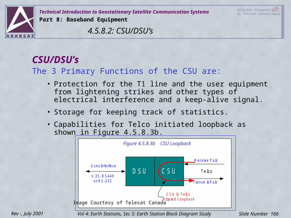
Technical Introduction to Geostationary Satellite Communication Systems Original Prepared by Telesat Canada
Slide Number 166Rev -, July 2001
CSU/DSU’sThe 3 Primary Functions of the CSU are:
• Protection for the T1 line and the user equipment from lightening strikes and other types of electrical interference and a keep-alive signal.
• Storage for keeping track of statistics.
• Capabilities for Telco initiated loopback as shown in Figure 4.5.8.3b.
U ser In te rface
V.35, R S449or R S-232
DSU
R ece ive Pair
T ransm it Pa ir
Te lcoCSU
C SU In T elcoIn itia ted Loopback
Figure 4.5.8.3b CSU Loopback
Image Courtesy of Telesat Canada
Part 8: Baseband Equipment
4.5.8.2: CSU/DSU’s
Vol 4: Earth Stations, Sec 5: Earth Station Block Diagram Study
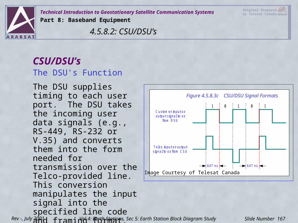
Technical Introduction to Geostationary Satellite Communication Systems Original Prepared by Telesat Canada
Slide Number 167Rev -, July 2001
CSU/DSU’sThe DSU's Function
The DSU supplies timing to each user port. The DSU takes the incoming user data signals (e.g., RS-449, RS-232 or V.35) and converts them into the form needed for transmission over the Telco-provided line. This conversion manipulates the input signal into the specified line code and framing format. Refer to Figure 4.5.8.3c for Signal Formats between the DSU and CSU sides.
0 1 0 11
647 ns647 ns
C ustom er input oroutput s igna l to or
from D SU
Telco input or outputs igna l to or from C SU
Figure 4.5.8.3c CSU/DSU Signal Formats
Image Courtesy of Telesat Canada
Part 8: Baseband Equipment
4.5.8.2: CSU/DSU’s
Vol 4: Earth Stations, Sec 5: Earth Station Block Diagram Study
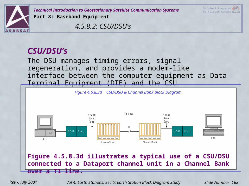
Technical Introduction to Geostationary Satellite Communication Systems Original Prepared by Telesat Canada
Slide Number 168Rev -, July 2001
CSU/DSU’s
DTEChannel BankChannel Bank
DS U
4 w irelocalloop
CS U DS U
4 w irelocalloop
C S U
DTE
T 1 L ine
Figure 4.5.8.3d CSU/DSU & Channel Bank Block Diagram
The DSU manages timing errors, signal regeneration, and provides a modem-like interface between the computer equipment as Data Terminal Equipment (DTE) and the CSU.
Figure 4.5.8.3d illustrates a typical use of a CSU/DSU connected to a Dataport channel unit in a Channel Bank over a T1 line.
Part 8: Baseband Equipment
4.5.8.2: CSU/DSU’s
Vol 4: Earth Stations, Sec 5: Earth Station Block Diagram Study
Technical Introduction to Geostationary Satellite Communication Systems Original Prepared by Telesat Canada
Slide Number 169Rev -, July 2001
Channel BanksA channel bank is a device at a telephone company central office (public exchange) that converts analog signals from home and business users into digital signals to be carried over higher speed lines between the central office and other exchanges.
The analog signal is converted into digital format as a 64 kbps PCM format known as a DS0.
This DS0 signal is then time division multiplexed with other DS0 signals to a T1 data rate.
A basic digital channel bank consists of 24 DS0’s called a digroup.
Many manufacturers package 2 digroups in a 48 channel framework.
Part 8: Baseband Equipment
4.5.8.3: Channel Banks
Vol 4: Earth Stations, Sec 5: Earth Station Block Diagram Study
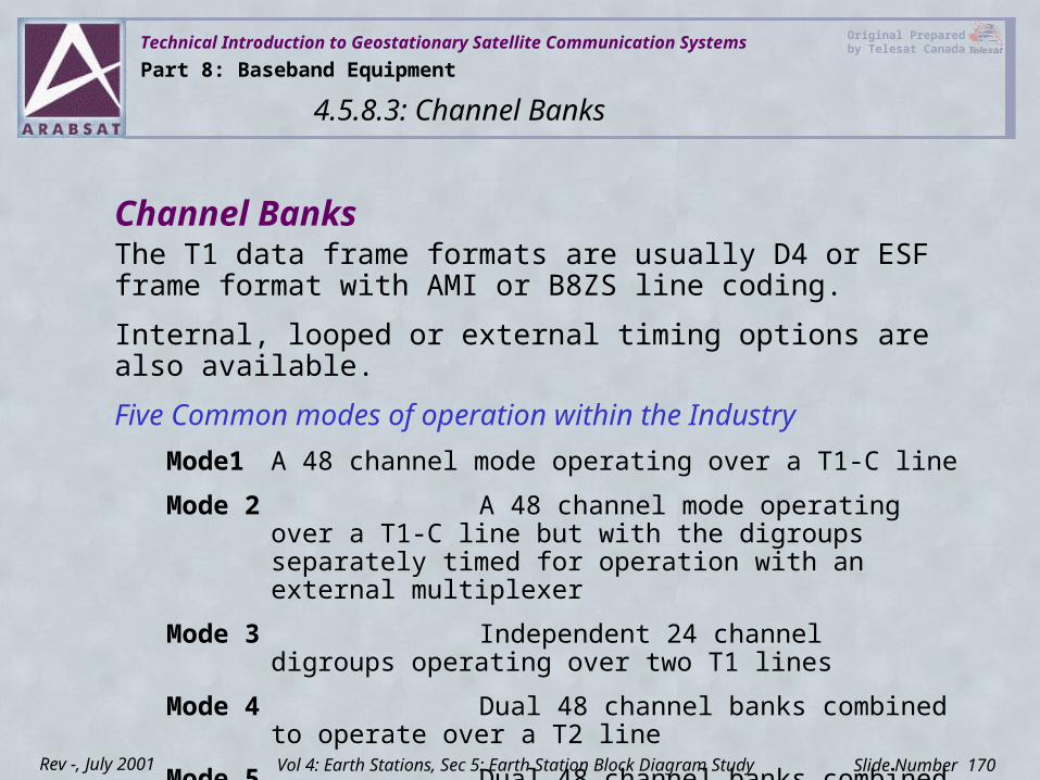
Technical Introduction to Geostationary Satellite Communication Systems Original Prepared by Telesat Canada
Slide Number 170Rev -, July 2001
Channel BanksThe T1 data frame formats are usually D4 or ESF frame format with AMI or B8ZS line coding.
Internal, looped or external timing options are also available.
Five Common modes of operation within the IndustryMode1 A 48 channel mode operating over a T1-C line
Mode 2 A 48 channel mode operating over a T1-C line but with the digroups separately timed for operation with an external multiplexer
Mode 3 Independent 24 channel digroups operating over two T1 lines
Mode 4 Dual 48 channel banks combined to operate over a T2 line
Mode 5 Dual 48 channel banks combined to operate over a fiber optic pair
Part 8: Baseband Equipment
4.5.8.3: Channel Banks
Vol 4: Earth Stations, Sec 5: Earth Station Block Diagram Study
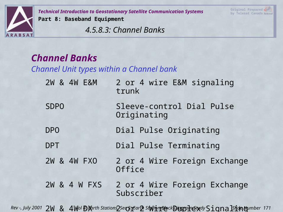
Technical Introduction to Geostationary Satellite Communication Systems Original Prepared by Telesat Canada
Slide Number 171Rev -, July 2001
Channel BanksChannel Unit types within a Channel bank
2W & 4W E&M 2 or 4 wire E&M signaling trunk
SDPO Sleeve-control Dial Pulse Originating
DPO Dial Pulse Originating
DPT Dial Pulse Terminating
2W & 4W FXO 2 or 4 Wire Foreign Exchange Office
2W & 4 W FXS 2 or 4 Wire Foreign Exchange Subscriber
2W & 4W DX 2 or 2 Wire Duplex Signaling
2W & 4W ETO 2 or 4 Wire Equalized Transmission Only
Part 8: Baseband Equipment
4.5.8.3: Channel Banks
Vol 4: Earth Stations, Sec 5: Earth Station Block Diagram Study
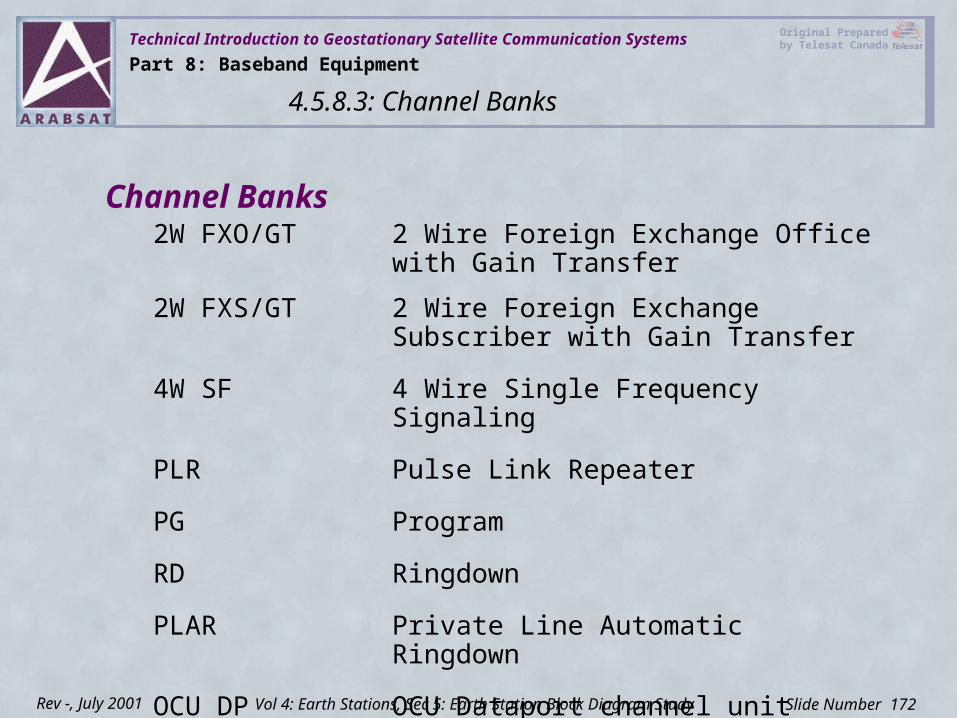
Technical Introduction to Geostationary Satellite Communication Systems Original Prepared by Telesat Canada
Slide Number 172Rev -, July 2001
2W FXO/GT 2 Wire Foreign Exchange Office with Gain Transfer
2W FXS/GT 2 Wire Foreign Exchange Subscriber with Gain Transfer
4W SF 4 Wire Single Frequency Signaling
PLR Pulse Link Repeater
PG Program
RD Ringdown
PLAR Private Line Automatic Ringdown
OCU DP OCU Dataport channel unit
Channel Banks
Part 8: Baseband Equipment
4.5.8.3: Channel Banks
Vol 4: Earth Stations, Sec 5: Earth Station Block Diagram Study
Technical Introduction to Geostationary Satellite Communication Systems Original Prepared by Telesat Canada
Slide Number 173Rev -, July 2001
Channel BanksIntelligent Channel Bank
Newer generation channel banks offer remote access and configuration.
Through a controller channel unit, control settings and options can be adjusted remotely or locally.
With remote interface capability, transmission levels may be adjusted and other maintenance or corrective action can be made without requiring a technician at a location, reducing maintenance costs of the system.
Part 8: Baseband Equipment
4.5.8.3: Channel Banks
Vol 4: Earth Stations, Sec 5: Earth Station Block Diagram Study
Technical Introduction to Geostationary Satellite Communication Systems Original Prepared by Telesat Canada
Slide Number 174Rev -, July 2001
Routers & HubsRoutersOn the Internet, a router is a device or, possibly just software in a computer, that directs information packets to the next point toward their destination.
The router is connected to at least two networks and decides which way to send each information packet based on its current understanding of the state of the networks to which it is connected.
A router is located at any gateway (where one network meets another), including each Internet point-of-presence.
A router is often included as part of a network switch.
A router creates or maintains a table of the available routes and their conditions and uses this information, along with distance and cost algorithms, to determine the best route for a given packet.
Part 8: Baseband Equipment
4.5.8.4: Routers & Hubs
Vol 4: Earth Stations, Sec 5: Earth Station Block Diagram Study
Technical Introduction to Geostationary Satellite Communication Systems Original Prepared by Telesat Canada
Slide Number 175Rev -, July 2001
Routers & HubsTypically, a packet may travel through a number of routers before arriving at its destination.
Very little filtering of data is done through routers. Routers do not care about the type of data they handle.
The router reads the network layer address of all packets transmitted by a network and forwards only those addressed to another network in its domain.
A router is often packaged in devices that perform other functions, such as aggregating data and selecting bandwidth requirements.
A router may perform routing of data on networks other than the Internet, including private corporate networks.
Routers operate at the network layer (layer 3) of the ISO Open Systems Interconnection--Reference Model.
Part 8: Baseband Equipment
4.5.8.4: Routers & Hubs
Vol 4: Earth Stations, Sec 5: Earth Station Block Diagram Study
Technical Introduction to Geostationary Satellite Communication Systems Original Prepared by Telesat Canada
Slide Number 176Rev -, July 2001
Routers & HubsA layer-3 switch is a switch that can perform routing functions. Types of RoutersAn edge router is a router that interfaces with an asynchronous transfer mode (ATM) network. A brouter is a network bridge combined with a router.What to Look for in a Router
• Type of router such as single protocol or multiprotocol, LAN or WAN, bridging router etc.
• Type of networks connected• Protocols supported• Transmission speed 1200 bits to several megabits• Number of ports• Interfaces supported for LANs & WANs• Network monitoring & management capabilities
Part 8: Baseband Equipment
4.5.8.4: Routers & Hubs
Vol 4: Earth Stations, Sec 5: Earth Station Block Diagram Study
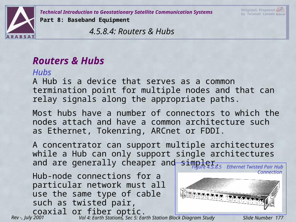
Technical Introduction to Geostationary Satellite Communication Systems Original Prepared by Telesat Canada
Slide Number 177Rev -, July 2001
Routers & HubsHubsA Hub is a device that serves as a common termination point for multiple nodes and that can relay signals along the appropriate paths.
Most hubs have a number of connectors to which the nodes attach and have a common architecture such as Ethernet, Tokenring, ARCnet or FDDI.
A concentrator can support multiple architectures while a Hub can only support single architectures and are generally cheaper and simpler. Figure 4.5.8.5 Ethernet Twisted Pair Hub
Connection Hub-node connections for a particular network must all use the same type of cable such as twisted pair, coaxial or fiber optic.
Part 8: Baseband Equipment
4.5.8.4: Routers & Hubs
Vol 4: Earth Stations, Sec 5: Earth Station Block Diagram Study
Technical Introduction to Geostationary Satellite Communication Systems Original Prepared by Telesat Canada
Slide Number 178Rev -, July 2001
Routers & HubsHub Features
• Hubs may be passive or active
• Passive Hubs do not change the signal in any way (non-repeating) and generally only support distances of up to 30 meters
• Active hubs require power supplies to boost/clean signals and support greater distances than passive hubs
• Some hubs offer network management capabilities
• Could include an onboard processor for monitoring Hub activity and can store monitoring data in a MIB (Management Information Base)
• Most Hubs have LEDs indicating the status of each port
• Many Hubs can do partitioning, which is a way to isolate or remove a faulty port or non functioning node from the Hub
Part 8: Baseband Equipment
4.5.8.4: Routers & Hubs
Vol 4: Earth Stations, Sec 5: Earth Station Block Diagram Study
Technical Introduction to Geostationary Satellite Communication Systems Original Prepared by Telesat Canada
Slide Number 179Rev -, July 2001
PBX EquipmentA PBX (private branch exchange) is a telephone system within a customer’s location that switches calls between its internal users on local lines while allowing all users to share a certain number of external phone lines.
The main purpose of a PBX is to save the cost of requiring a line for each user to the telephone company's central office.
Part 8: Baseband Equipment
4.5.8.5: PBX Equipment
Vol 4: Earth Stations, Sec 5: Earth Station Block Diagram Study
Technical Introduction to Geostationary Satellite Communication Systems Original Prepared by Telesat Canada
Slide Number 180Rev -, July 2001
Dialing Schemes
• A PBX allows four-digit dialing for local extension numbers
• Single digit access, e.g. “9” to access outgoing trunks, “8” to access tie trunks. (Tie trunks are privately owned or leased lines used to interconnect PBX’s together.)
• Single digit access for special trunks such as WATS, foreign exchange and 800 numbers. To access these lines, many PBXs offer least cost routing (LCR) features to enable the PBX to determine the most economical route based on the class of trunks terminated, their busy/idle status and the station line class.
PBX Equipment
Part 8: Baseband Equipment
4.5.8.5: PBX Equipment
Vol 4: Earth Stations, Sec 5: Earth Station Block Diagram Study
Technical Introduction to Geostationary Satellite Communication Systems Original Prepared by Telesat Canada
Slide Number 181Rev -, July 2001
PBX EquipmentThe PBX is typically owned and operated by the customer rather than the telephone company.
PBX’s can use analog or digital phones.
• With an analog phone, the analog-to-digital conversion is made at the PBX
• With a digital phone, the analog-to-digital conversion is made in the telephone itself
Part 8: Baseband Equipment
4.5.8.5: PBX Equipment
Vol 4: Earth Stations, Sec 5: Earth Station Block Diagram Study
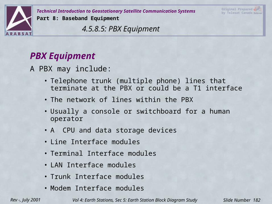
Technical Introduction to Geostationary Satellite Communication Systems Original Prepared by Telesat Canada
Slide Number 182Rev -, July 2001
A PBX may include: • Telephone trunk (multiple phone) lines that terminate at the PBX
or could be a T1 interface
• The network of lines within the PBX
• Usually a console or switchboard for a human operator
• A CPU and data storage devices
• Line Interface modules
• Terminal Interface modules
• LAN Interface modules
• Trunk Interface modules
• Modem Interface modules
PBX Equipment
Part 8: Baseband Equipment
4.5.8.5: PBX Equipment
Vol 4: Earth Stations, Sec 5: Earth Station Block Diagram Study
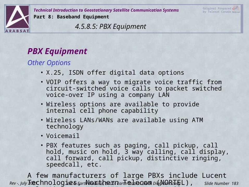
Technical Introduction to Geostationary Satellite Communication Systems Original Prepared by Telesat Canada
Slide Number 183Rev -, July 2001
PBX EquipmentOther Options
• X.25, ISDN offer digital data options• VOIP offers a way to migrate voice traffic from circuit-switched
voice calls to packet switched voice-over IP using a company LAN• Wireless options are available to provide internal cell phone
capability • Wireless LANs/WANs are available using ATM technology• Voicemail• PBX features such as paging, call pickup, call hold, music on hold,
3 way calling, call display, call forward, call pickup, distinctive ringing, speedcall, etc.
A few manufacturers of large PBXs include Lucent Technologies, Northern Telecom (NORTEL), Rolm/Siemens, NEC, GTE, Intecom, Fujitsu, Hitachi, and Mitel.
Part 8: Baseband Equipment
4.5.8.5: PBX Equipment
Vol 4: Earth Stations, Sec 5: Earth Station Block Diagram Study
Technical Introduction to Geostationary Satellite Communication Systems Original Prepared by Telesat Canada
Slide Number 184Rev -, July 2001
Redundancy EquipmentPart 9
Vol 4: Earth Stations
4.5: Earth Station Block Diagram Study
Technical Introduction to Geostationary Satellite Communication Systems Original Prepared by Telesat Canada
Slide Number 185Rev -, July 2001
Contents
4.5.9.1 The Redundancy Function4.5.9.2 Monitor & Control Panels4.5.9.3 Coax and Waveguide Switches4.5.9.4 Network Control Systems (NCS)4.5.9.5 Remote Terminal Units (RTU)4.5.9.6 PBX Equipment
Vol 4: Earth Stations
4.5: Earth Station Block Diagram Study
Technical Introduction to Geostationary Satellite Communication Systems Original Prepared by Telesat Canada
Slide Number 186Rev -, July 2001
The Redundancy FunctionRedundancy is provided to improve service reliability and offer a non-interruptive maintenance lineup to the on/offline equipment.
Redundancy can be provided in several ways in an Earth Station:• Baseband redundancy • RF equipment redundancy
• IF equipment (Modem) redundancy • Entire chain redundancy
Redundancy can be offered in hot standby (TWTA or Klystron pushing RF power into a dummy load) or cold.
Redundancy can also be offered in 1 for 1 or 1 for N where N could be any number of online chains that can be captured by the standby.
Various equipment manufacturers offer many varieties of equipment to provide automatic capture of the online chain.
Part 9: Redundancy Equipment
4.5.9.1: The Redundancy Function
Vol 4: Earth Stations, Sec 5: Earth Station Block Diagram Study
Technical Introduction to Geostationary Satellite Communication Systems Original Prepared by Telesat Canada
Slide Number 187Rev -, July 2001
Monitor & Control (MAC) PanelsMAC panels monitor and control Earth Station Equipment.
Many MAC Systems are custom designed to fit the specific needs of the Earth Station hardware environment.
Each piece of equipment to be monitored must extend its status and control points so that the MAC can supervise its health and then make decisions to switch when the unit becomes faulty.
Typical Alarm Points include
Power supply faultsFan FaultLow & Hi RF powerUC or DC faultsHPA FaultsTemperature Faults Chain Fail StatusLNA Fault
Typical Control points include
HPA InhibitFault Reset on HPA HPA Auto/ManualForce Chain SwitchForce LNA Switch
Part 9: Redundancy Equipment
4.5.9.2: Monitor & Control (MAC) Panels
Vol 4: Earth Stations, Sec 5: Earth Station Block Diagram Study
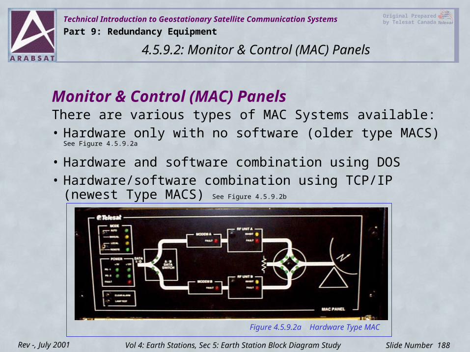
Technical Introduction to Geostationary Satellite Communication Systems Original Prepared by Telesat Canada
Slide Number 188Rev -, July 2001
Monitor & Control (MAC) PanelsThere are various types of MAC Systems available:• Hardware only with no software (older type MACS) See Figure 4.5.9.2a
• Hardware and software combination using DOS• Hardware/software combination using TCP/IP (newest Type
MACS) See Figure 4.5.9.2b
Figure 4.5.9.2a Hardware Type MAC
Part 9: Redundancy Equipment
4.5.9.2: Monitor & Control (MAC) Panels
Vol 4: Earth Stations, Sec 5: Earth Station Block Diagram Study
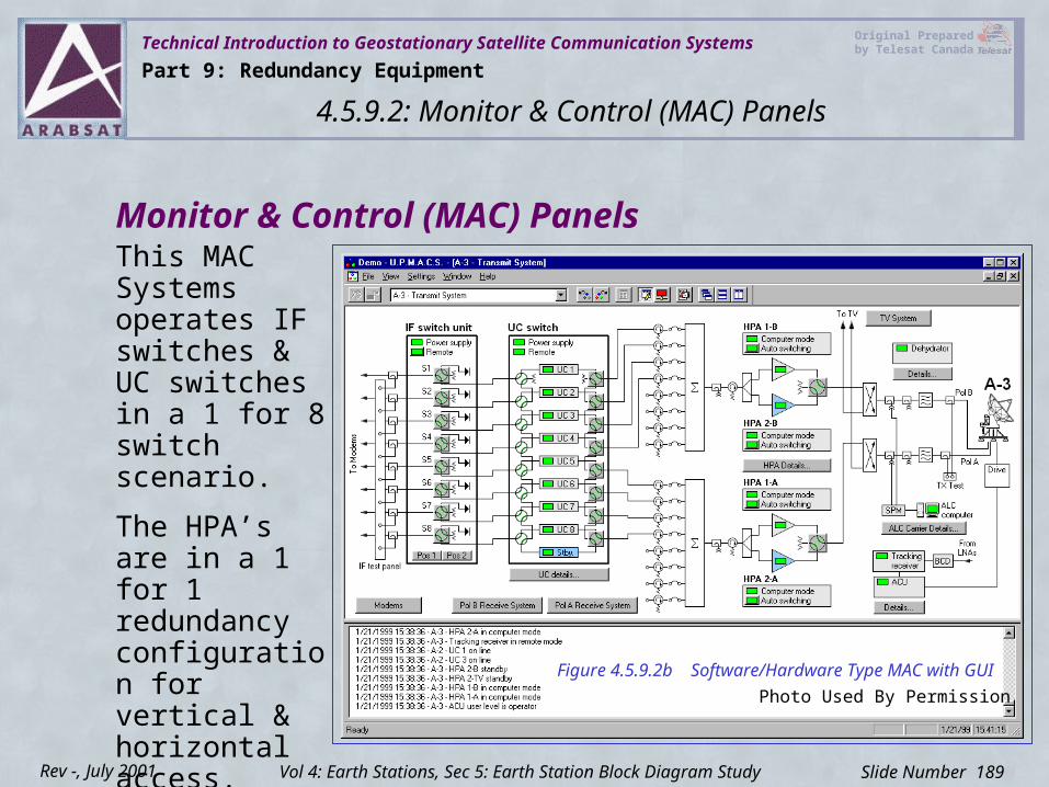
Technical Introduction to Geostationary Satellite Communication Systems Original Prepared by Telesat Canada
Slide Number 189Rev -, July 2001
Monitor & Control (MAC) PanelsThis MAC Systems operates IF switches & UC switches in a 1 for 8 switch scenario.
The HPA’s are in a 1 for 1 redundancy configuration for vertical & horizontal access. Figure 4.5.9.2b Software/Hardware Type MAC with GUI
Photo Used By Permission
Part 9: Redundancy Equipment
4.5.9.2: Monitor & Control (MAC) Panels
Vol 4: Earth Stations, Sec 5: Earth Station Block Diagram Study
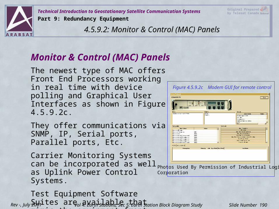
Technical Introduction to Geostationary Satellite Communication Systems Original Prepared by Telesat Canada
Slide Number 190Rev -, July 2001
Monitor & Control (MAC) PanelsThe newest type of MAC offers Front End Processors working in real time with device polling and Graphical User Interfaces as shown in Figure 4.5.9.2c.
They offer communications via SNMP, IP, Serial ports, Parallel ports, Etc.
Carrier Monitoring Systems can be incorporated as well as Uplink Power Control Systems.
Test Equipment Software Suites are available that mimic the equipment front panel on the GUI, facilitating unit control.
Figure 4.5.9.2c Modem GUI for remote control
Photos Used By Permission of Industrial LogicCorporation
Part 9: Redundancy Equipment
4.5.9.2: Monitor & Control (MAC) Panels
Vol 4: Earth Stations, Sec 5: Earth Station Block Diagram Study
Technical Introduction to Geostationary Satellite Communication Systems Original Prepared by Telesat Canada
Slide Number 191Rev -, July 2001
Alarms can be priority controlled and set to trigger events, messages, or even send email.
Report generation is made easy and can be filtered to list just specific events, sites or equipment.
With today’s software anything can be achieved making monitoring the most sophisticated Earth Station a much less complicated chore.
Monitor & Control (MAC) Panels
Part 9: Redundancy Equipment
4.5.9.2: Monitor & Control (MAC) Panels
Vol 4: Earth Stations, Sec 5: Earth Station Block Diagram Study
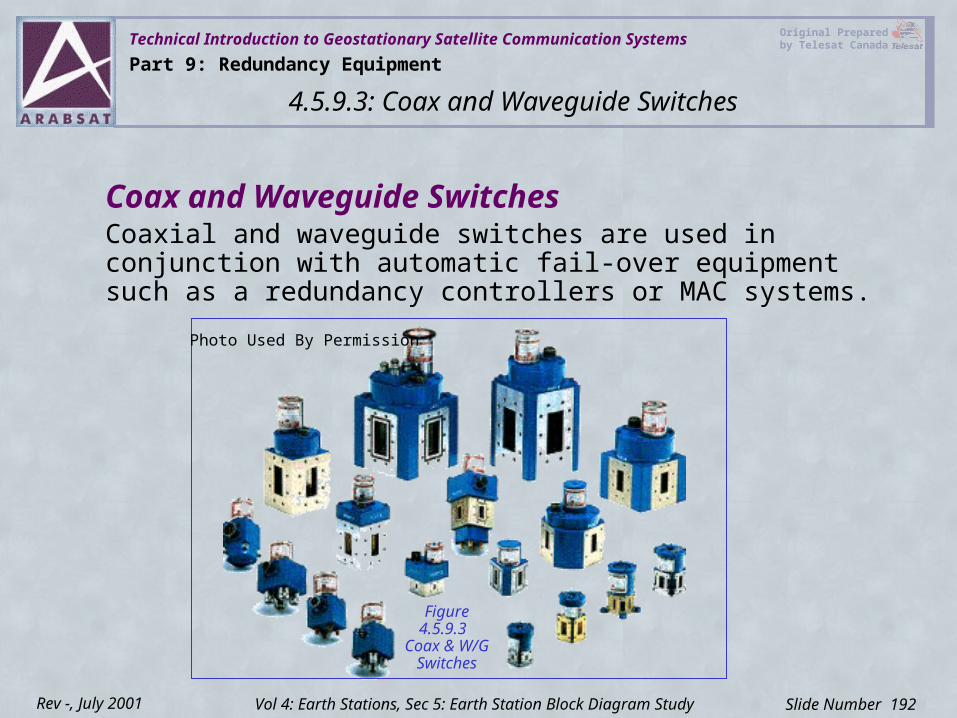
Technical Introduction to Geostationary Satellite Communication Systems Original Prepared by Telesat Canada
Slide Number 192Rev -, July 2001
Coax and Waveguide SwitchesCoaxial and waveguide switches are used in conjunction with automatic fail-over equipment such as a redundancy controllers or MAC systems.
Figure 4.5.9.3
Coax & W/G Switches
Part 9: Redundancy Equipment
4.5.9.3: Coax and Waveguide Switches
Vol 4: Earth Stations, Sec 5: Earth Station Block Diagram Study
Photo Used By Permission
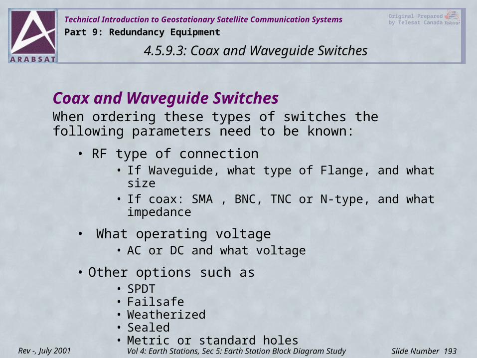
Technical Introduction to Geostationary Satellite Communication Systems Original Prepared by Telesat Canada
Slide Number 193Rev -, July 2001
When ordering these types of switches the following parameters need to be known:
• RF type of connection • If Waveguide, what type of Flange, and what size• If coax: SMA , BNC, TNC or N-type, and what impedance
• What operating voltage • AC or DC and what voltage
• Other options such as• SPDT• Failsafe• Weatherized• Sealed• Metric or standard holes
Coax and Waveguide Switches
Part 9: Redundancy Equipment
4.5.9.3: Coax and Waveguide Switches
Vol 4: Earth Stations, Sec 5: Earth Station Block Diagram Study
Technical Introduction to Geostationary Satellite Communication Systems Original Prepared by Telesat Canada
Slide Number 194Rev -, July 2001
Coax and Waveguide SwitchesCoaxial and waveguide switches typically have a life from 200,000 to 500,000 cycles.
RF power capability is typically half the power of the guide rating.
Waveguide switches can be pressurized up to 30 psi.
Some switches have a manual path override and RF path indication.
Part 9: Redundancy Equipment
4.5.9.3: Coax and Waveguide Switches
Vol 4: Earth Stations, Sec 5: Earth Station Block Diagram Study
Technical Introduction to Geostationary Satellite Communication Systems Original Prepared by Telesat Canada
Slide Number 195Rev -, July 2001
Network Control Systems (NCS)Most Network Control Systems are specialized software-based computer systems with multiple Graphical User Interfaces designed specifically to monitor and control specialized telecommunication networks.
This windows based platform is a multitasking computer available to run entire communication networks and is usually equipped with redundancy in case of a failure.
Hierarchy screens are usually available depending on logon privileges.
Security access is defined by granting various levels of access to different users.
Part 9: Redundancy Equipment
4.5.9.4: Network Control Systems (NCS)
Vol 4: Earth Stations, Sec 5: Earth Station Block Diagram Study
Technical Introduction to Geostationary Satellite Communication Systems Original Prepared by Telesat Canada
Slide Number 196Rev -, July 2001
Hierarchy screens may include:
Configuration Management Equipment configuration details
Overview Management Overview of equipment configuration details
Database Management Various new & old and backup databases
Operation Management Statistics, control, debug, status details, reports
Software Upgrades List of patches applied and software revision levels
Administration Security, access lists , etc.
Network Control Systems (NCS)
Part 9: Redundancy Equipment
4.5.9.4: Network Control Systems (NCS)
Vol 4: Earth Stations, Sec 5: Earth Station Block Diagram Study
Technical Introduction to Geostationary Satellite Communication Systems Original Prepared by Telesat Canada
Slide Number 197Rev -, July 2001
Remote Terminal Units (RTU)Remote Terminal Units could be standalone Monitor and Control Systems.
RTU’s contain all the status and control points that a M&C system does.
They report information to a Central Monitor and Control Panel within the Earth Station, and also report it to a Master Network Control Center for monitor and control.
Depending which site location wishes to control the site, the MAC equipment must be placed in Local or Remote control.
RTU is a term used back in the 1970 to 1980 era. It is seldom used today as it is replaced by a more modern M&C systems connected by LAN’s and WAN’s.
Part 9: Redundancy Equipment
4.5.9.5: Remote Terminal Units (RTU)
Vol 4: Earth Stations, Sec 5: Earth Station Block Diagram Study
Technical Introduction to Geostationary Satellite Communication Systems Original Prepared by Telesat Canada
Slide Number 198Rev -, July 2001
Passive DevicesPart 10
Vol 4: Earth Stations
4.5: Earth Station Block Diagram Study
Technical Introduction to Geostationary Satellite Communication Systems Original Prepared by Telesat Canada
Slide Number 199Rev -, July 2001
Contents
4.5.10.1 Waveguide - Terminations- Circulators- Hybrid Coupler- Crossguide Couplers- Tuned Devices (Filters)
4.5.10.2 Coaxial - Splitters & Combiners- RF Cables and their characteristics
Vol 4: Earth Stations
4.5: Earth Station Block Diagram Study
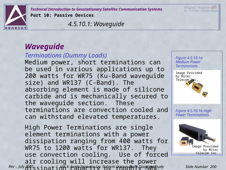
Technical Introduction to Geostationary Satellite Communication Systems Original Prepared by Telesat Canada
Slide Number 200Rev -, July 2001
WaveguideTerminations (Dummy Loads)Medium power, short terminations can be used in various applications up to 200 watts for WR75 (Ku-Band waveguide size) and WR137 (C-Band). The absorbing element is made of silicone carbide and is mechanically secured to the waveguide section. These terminations are convection cooled and can withstand elevated temperatures.
High Power Terminations are single element terminations with a power dissipation ranging from 400 watts for WR75 to 1200 watts for WR137. They use convection cooling. Use of forced air cooling will increase the power dissipation capacity by roughly 50%. Higher ratings can be achieved by making changes to the heat dissipation fins.
Figure 4.5.10.1a Medium Power Terminations
Figure 4.5.10.1b High Power Terminations
Image Provided by Mitec Telecom Inc.
Image Provided by Mitec Telecom Inc.
Part 10: Passive Devices
4.5.10.1: Waveguide
Vol 4: Earth Stations, Sec 5: Earth Station Block Diagram Study
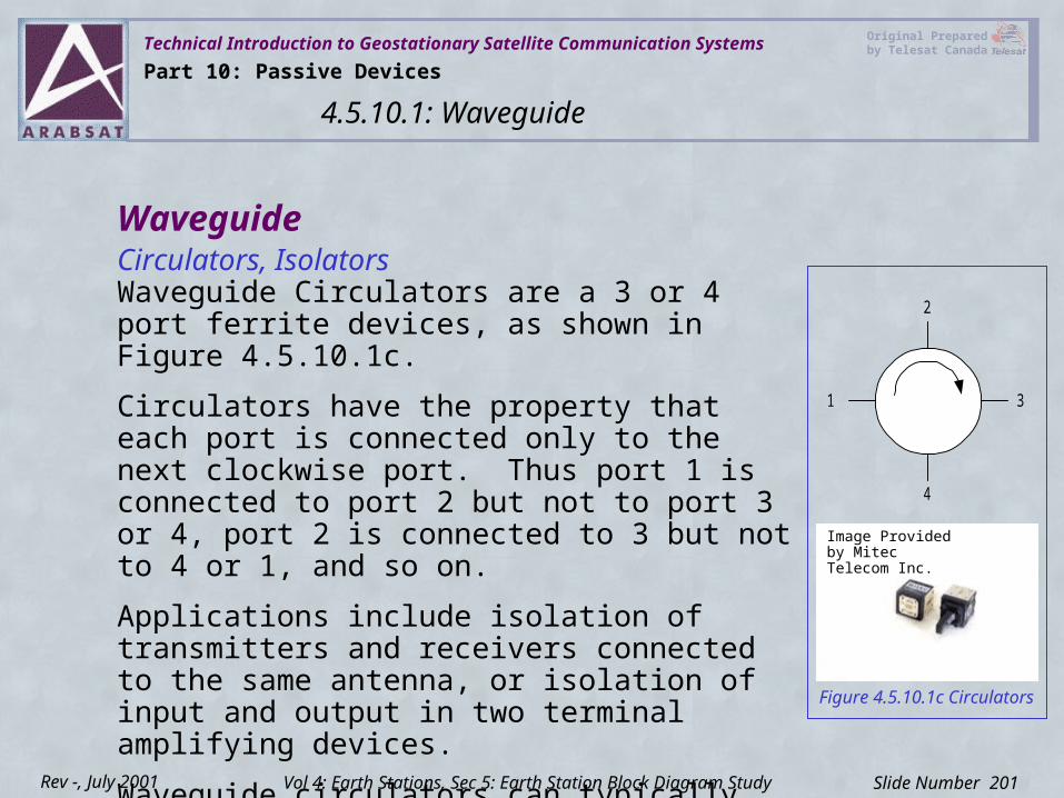
Technical Introduction to Geostationary Satellite Communication Systems Original Prepared by Telesat Canada
Slide Number 201Rev -, July 2001
WaveguideCirculators, IsolatorsWaveguide Circulators are a 3 or 4 port ferrite devices, as shown in Figure 4.5.10.1c.
Circulators have the property that each port is connected only to the next clockwise port. Thus port 1 is connected to port 2 but not to port 3 or 4, port 2 is connected to 3 but not to 4 or 1, and so on.
Applications include isolation of transmitters and receivers connected to the same antenna, or isolation of input and output in two terminal amplifying devices.
Waveguide circulators can typically offer approximately 26 to 30 dB of port isolation with a insertion loss of approximately 0.2 dB.
Figure 4.5.10.1c Circulators
1
2
3
4
Image Provided by Mitec Telecom Inc.
Part 10: Passive Devices
4.5.10.1: Waveguide
Vol 4: Earth Stations, Sec 5: Earth Station Block Diagram Study
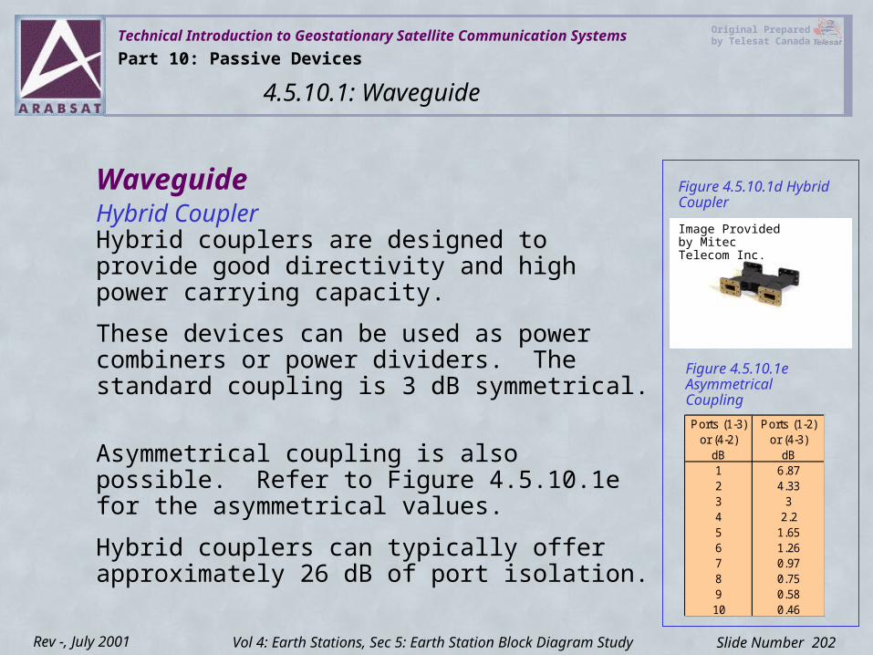
Technical Introduction to Geostationary Satellite Communication Systems Original Prepared by Telesat Canada
Slide Number 202Rev -, July 2001
WaveguideHybrid CouplerHybrid couplers are designed to provide good directivity and high power carrying capacity.
These devices can be used as power combiners or power dividers. The standard coupling is 3 dB symmetrical.
Asymmetrical coupling is also possible. Refer to Figure 4.5.10.1e for the asymmetrical values.
Hybrid couplers can typically offer approximately 26 dB of port isolation.
Figure 4.5.10.1d Hybrid Coupler
Ports (1-3) Ports (1-2)or (4-2) or (4-3)
dB dB1 6.872 4.333 34 2.25 1.656 1.267 0.978 0.759 0.5810 0.46
Figure 4.5.10.1e Asymmetrical Coupling
Image Provided by Mitec Telecom Inc.
Part 10: Passive Devices
4.5.10.1: Waveguide
Vol 4: Earth Stations, Sec 5: Earth Station Block Diagram Study
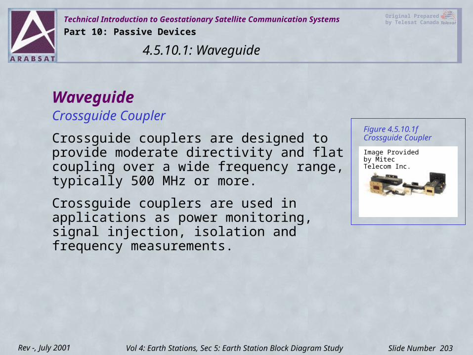
Technical Introduction to Geostationary Satellite Communication Systems Original Prepared by Telesat Canada
Slide Number 203Rev -, July 2001
WaveguideCrossguide Coupler
Crossguide couplers are designed to provide moderate directivity and flat coupling over a wide frequency range, typically 500 MHz or more.
Crossguide couplers are used in applications as power monitoring, signal injection, isolation and frequency measurements.
Figure 4.5.10.1f Crossguide Coupler
Image Provided by Mitec Telecom Inc.
Part 10: Passive Devices
4.5.10.1: Waveguide
Vol 4: Earth Stations, Sec 5: Earth Station Block Diagram Study
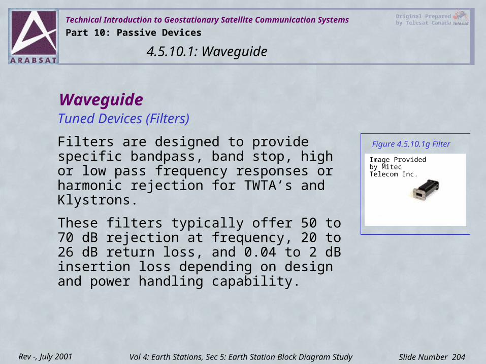
Technical Introduction to Geostationary Satellite Communication Systems Original Prepared by Telesat Canada
Slide Number 204Rev -, July 2001
WaveguideTuned Devices (Filters)
Filters are designed to provide specific bandpass, band stop, high or low pass frequency responses or harmonic rejection for TWTA’s and Klystrons.
These filters typically offer 50 to 70 dB rejection at frequency, 20 to 26 dB return loss, and 0.04 to 2 dB insertion loss depending on design and power handling capability.
Figure 4.5.10.1g Filter
Image Provided by Mitec Telecom Inc.
Part 10: Passive Devices
4.5.10.1: Waveguide
Vol 4: Earth Stations, Sec 5: Earth Station Block Diagram Study
Technical Introduction to Geostationary Satellite Communication Systems Original Prepared by Telesat Canada
Slide Number 205Rev -, July 2001
CoaxialSplitters & CombinersSplitters/Combiners are reciprocal devices and as such can be used to combine or split the signal.
Most splitters and combiners are passive devices that accept an input signal and deliver multiple output signals.
The output signals would have specific phase and amplitude characteristics. The ideal splitter will offer equal amplitude and 0° phase relationship between any two output signals. Splitters with 180° phase are available.
Isolation between each output port is typically 20 to 35 dB depending on frequency and manufacturing techniques.
It is important to terminate unused ports if high isolation is required between ports. All Ports must be properly impedance matched to reduce reflections.
Part 10: Passive Devices
4.5.10.2: Coaxial
Vol 4: Earth Stations, Sec 5: Earth Station Block Diagram Study
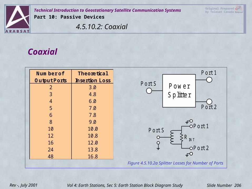
Technical Introduction to Geostationary Satellite Communication Systems Original Prepared by Telesat Canada
Slide Number 206Rev -, July 2001
Number of TheoreticalOutput Ports Insertion Loss
2 3.03 4.84 6.05 7.06 7.88 9.0
10 10.012 10.816 12.024 13.848 16.8
Figure 4.5.10.2a Splitter Losses for Number of Ports
PowerSp litte r
Port S
Port 1
Port 2
Port SPort 1
Port 2
R IN T
Coaxial
Part 10: Passive Devices
4.5.10.2: Coaxial
Vol 4: Earth Stations, Sec 5: Earth Station Block Diagram Study
Technical Introduction to Geostationary Satellite Communication Systems Original Prepared by Telesat Canada
Slide Number 207Rev -, July 2001
CoaxialRF Cables & their CharacteristicsCoaxial cables consist of one or more center conductors surrounded by a shield of flexible braid or semi rigid copper or aluminum foil, with a outer jacket of PVC or Teflon.
Coaxial jacket can be made from various materials:• PVC for general purpose indoor projects
• Armour plated - for heavy duty industrial applications
• Teflon - for extreme temperature or chemical environments, good for plenums and riser environments
• Direct burial - may have flooding compounds or tougher jacket
• Aerial applications - usually has a stiff strong conductor attached to the coax cable for hanging from poles, buildings etc.
Part 10: Passive Devices
4.5.10.2: Coaxial
Vol 4: Earth Stations, Sec 5: Earth Station Block Diagram Study
Technical Introduction to Geostationary Satellite Communication Systems Original Prepared by Telesat Canada
Slide Number 208Rev -, July 2001
Special precautions are required to avoid unwanted affects in installing coaxial cables. Cables must be grounded only in one place, so precautions are required to insulate connectors from ground.
Double shielding is used in heavy EMI (electromagnetic interference) areas.
Coaxial cable is used extensively in CATV (cable television), and telecommunication networks as it is relatively inexpensive, can be installed by moderately skilled workers, as has wide bandwidth properties.
Coaxial
Part 10: Passive Devices
4.5.10.2: Coaxial
Vol 4: Earth Stations, Sec 5: Earth Station Block Diagram Study
Technical Introduction to Geostationary Satellite Communication Systems Original Prepared by Telesat Canada
Slide Number 209Rev -, July 2001
CoaxialCoax supports video, data or both:
• Signal loss increases exponentially with frequency. Frequencies above 4 GHz generally require the use of waveguide from a transmission efficiency point of view
• Below 3 GHz coaxial cable is economically cheaper to use. Above this elliptical or waveguide is used for longer distances. Waveguide is better suited particularly at higher frequencies and can handle higher power levels
• Power rating of cable should not be exceeded or the dielectric properties of the cable breaks down and causes further problems
• Coax attenuation varies with temperature
• See the following chart for correction factor vs. temperature
Part 10: Passive Devices
4.5.10.2: Coaxial
Vol 4: Earth Stations, Sec 5: Earth Station Block Diagram Study
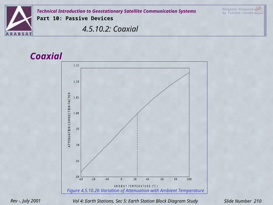
Technical Introduction to Geostationary Satellite Communication Systems Original Prepared by Telesat Canada
Slide Number 210Rev -, July 2001
Figure 4.5.10.2b Variation of Attenuation with Ambient Temperature
Coaxial
Part 10: Passive Devices
4.5.10.2: Coaxial
Vol 4: Earth Stations, Sec 5: Earth Station Block Diagram Study
1.15
1.10
1.05
1.00
.95
.90
.85
.80-60 -40-20 0 20 40 60 80 100
AMBIENT TEMPERATURE ( C)o
ATT
EN
UA
TIO
N C
OR
RE
CTI
ON
FA
CTO
R
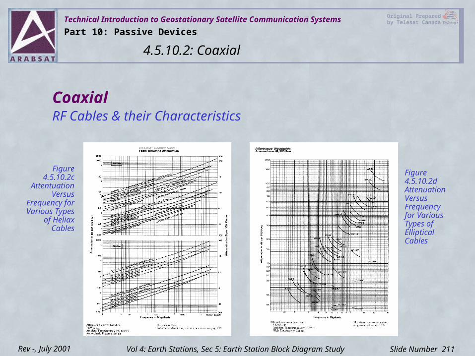
Technical Introduction to Geostationary Satellite Communication Systems Original Prepared by Telesat Canada
Slide Number 211Rev -, July 2001
Coaxial
Figure 4.5.10.2c
Attentuation Versus
Frequency for Various
Types of Heliax Cables
Figure 4.5.10.2d Attenuation Versus Frequency for Various Types of Elliptical Cables
RF Cables & their Characteristics
Part 10: Passive Devices
4.5.10.2: Coaxial
Vol 4: Earth Stations, Sec 5: Earth Station Block Diagram Study
Technical Introduction to Geostationary Satellite Communication Systems Original Prepared by Telesat Canada
Slide Number 212Rev -, July 2001
CoaxialRF Cables & their Characteristics
Common types of coaxial cables used are the RG series for 75 ohm applications: RG59, RG6, RG11, RG216.
For 50 ohm applications, common types of coaxial cables used in the communications industry are RG58, RG8, RG11, RG214 series.
A jump into the next series cable typically increases the center conductor outer diameter (OD), the jacket OD and decreases the loss in dB per 100ft for the associated frequency.
Part 10: Passive Devices
4.5.10.2: Coaxial
Vol 4: Earth Stations, Sec 5: Earth Station Block Diagram Study
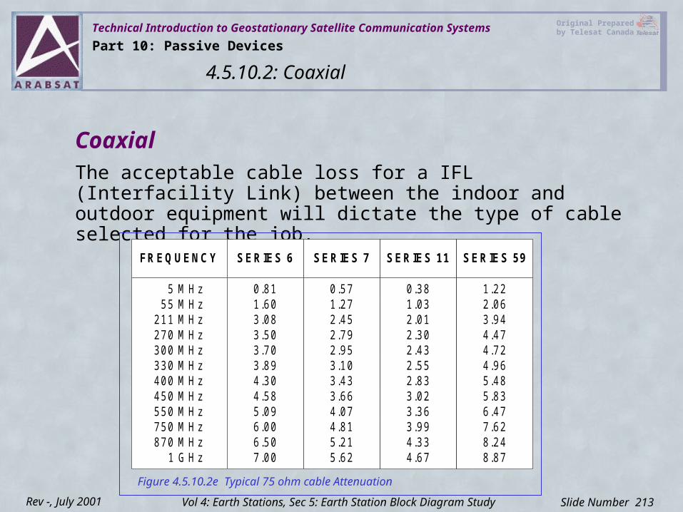
Technical Introduction to Geostationary Satellite Communication Systems Original Prepared by Telesat Canada
Slide Number 213Rev -, July 2001
The acceptable cable loss for a IFL (Interfacility Link) between the indoor and outdoor equipment will dictate the type of cable selected for the job.
Figure 4.5.10.2e Typical 75 ohm cable Attenuation
Coaxial
Part 10: Passive Devices
4.5.10.2: Coaxial
Vol 4: Earth Stations, Sec 5: Earth Station Block Diagram Study
FREQUENCY SERIES 6 SERIES 7 SERIES 11 SERIES 59
5 MHz55 MHz
211 MHz270 MHz300 MHz330 MHz400 MHz450 MHz550 MHz750 MHz870 MHz
1 GHz
0.811.603.083.503.703.894.304.585.096.006.507.00
0.571.272.452.792.953.103.433.664.074.815.215.62
0.381.032.012.302.432.552.833.023.363.994.334.67
1.222.063.944.474.724.965.485.836.477.628.248.87