Embed Size (px)
Citation preview

Convective Heat Transfer
Solved Problems
Michel Favre-Marinet Sedat Tardu

This page intentionally left blank
Convective Heat Transfer

This page intentionally left blank
Convective Heat Transfer
Solved Problems
Michel Favre-Marinet Sedat Tardu
First published in France in 2008 by Hermes Science/Lavoisier entitled: Écoulements avec échanges de chaleur volumes 1 et 2 © LAVOISIER, 2008 First published in Great Britain and the United States in 2009 by ISTE Ltd and John Wiley & Sons, Inc. Apart from any fair dealing for the purposes of research or private study, or criticism or review, as permitted under the Copyright, Designs and Patents Act 1988, this publication may only be reproduced, stored or transmitted, in any form or by any means, with the prior permission in writing of the publishers, or in the case of reprographic reproduction in accordance with the terms and licenses issued by the CLA. Enquiries concerning reproduction outside these terms should be sent to the publishers at the undermentioned address: ISTE Ltd John Wiley & Sons, Inc. 27-37 St George’s Road 111 River Street London SW19 4EU Hoboken, NJ 07030 UK USA
www.iste.co.uk www.wiley.com © ISTE Ltd, 2009 The rights of Michel Favre-Marinet and Sedat Tardu to be identified as the authors of this work have been asserted by them in accordance with the Copyright, Designs and Patents Act 1988.
Library of Congress Cataloging-in-Publication Data Favre-Marinet, Michel, 1947- [Ecoulements avec échanges de chaleur. English] Convective heat transfer : solved problems / Michel Favre-Marinet, Sedat Tardu. p. cm. Includes bibliographical references and index. ISBN 978-1-84821-119-3 1. Heat--Convection. 2. Heat--Transmission. I. Tardu, Sedat, 1959- II. Title. TJ260.F3413 2009 621.402'25--dc22
2009016463 British Library Cataloguing-in-Publication Data A CIP record for this book is available from the British Library ISBN: 978-1-84821-119-3
Printed and bound in Great Britain by CPI Antony Rowe, Chippenham and Eastbourne.
Table of Contents
Foreword. . . . . . . . . . . . . . . . . . . . . . . . . . . . . . . . . . . . . . . . . . xiii Preface . . . . . . . . . . . . . . . . . . . . . . . . . . . . . . . . . . . . . . . . . . . xv
Chapter 1. Fundamental Equations, Dimensionless Numbers . . . . . . . . 1
1.1. Fundamental equations . . . . . . . . . . . . . . . . . . . . . . . . . . . . . 1 1.1.1. Local equations . . . . . . . . . . . . . . . . . . . . . . . . . . . . . . . 1 1.1.2. Integral conservation equations. . . . . . . . . . . . . . . . . . . . . . 4 1.1.3. Boundary conditions . . . . . . . . . . . . . . . . . . . . . . . . . . . . 7 1.1.4. Heat-transfer coefficient . . . . . . . . . . . . . . . . . . . . . . . . . . 7
1.2. Dimensionless numbers . . . . . . . . . . . . . . . . . . . . . . . . . . . . 8 1.3. Flows with variable physical properties: heat transfer in a laminar Couette flow . . . . . . . . . . . . . . . . . . . . . . . . . . . . . . 9
1.3.1. Description of the problem . . . . . . . . . . . . . . . . . . . . . . . . 9 1.3.2. Guidelines . . . . . . . . . . . . . . . . . . . . . . . . . . . . . . . . . . 10 1.3.3. Solution. . . . . . . . . . . . . . . . . . . . . . . . . . . . . . . . . . . . 10
1.4. Flows with dissipation . . . . . . . . . . . . . . . . . . . . . . . . . . . . . 14 1.4.1. Description of the problem . . . . . . . . . . . . . . . . . . . . . . . . 14 1.4.2. Guidelines . . . . . . . . . . . . . . . . . . . . . . . . . . . . . . . . . . 14 1.4.3. Solution. . . . . . . . . . . . . . . . . . . . . . . . . . . . . . . . . . . . 15
1.5. Cooling of a sphere by a gas flow. . . . . . . . . . . . . . . . . . . . . . . 20 1.5.1. Description of the problem . . . . . . . . . . . . . . . . . . . . . . . . 20 1.5.2. Guidelines . . . . . . . . . . . . . . . . . . . . . . . . . . . . . . . . . . 21 1.5.3. Solution. . . . . . . . . . . . . . . . . . . . . . . . . . . . . . . . . . . . 21
vi Convective heat Transfer
Chapter 2. Laminar Fully Developed Forced Convection in Ducts . . . . . 31
2.1. Hydrodynamics . . . . . . . . . . . . . . . . . . . . . . . . . . . . . . . . . 31 2.1.1. Characteristic parameters . . . . . . . . . . . . . . . . . . . . . . . . . 31 2.1.2. Flow regions. . . . . . . . . . . . . . . . . . . . . . . . . . . . . . . . . 32
2.2. Heat transfer . . . . . . . . . . . . . . . . . . . . . . . . . . . . . . . . . . . 33 2.2.1. Thermal boundary conditions. . . . . . . . . . . . . . . . . . . . . . . 33 2.2.2. Bulk temperature . . . . . . . . . . . . . . . . . . . . . . . . . . . . . . 34 2.2.3. Heat-transfer coefficient . . . . . . . . . . . . . . . . . . . . . . . . . . 34 2.2.4. Fully developed thermal region . . . . . . . . . . . . . . . . . . . . . 34
2.3. Heat transfer in a parallel-plate channel with uniform wall heat flux . . 35 2.3.1. Description of the problem . . . . . . . . . . . . . . . . . . . . . . . . 35 2.3.2. Guidelines . . . . . . . . . . . . . . . . . . . . . . . . . . . . . . . . . . 36 2.3.3. Solution. . . . . . . . . . . . . . . . . . . . . . . . . . . . . . . . . . . . 37
2.4. Flow in a plane channel insulated on one side and heated at uniform temperature on the opposite side . . . . . . . . . . . . . . . . . . . . . . . . . . 46
2.4.1. Description of the problem . . . . . . . . . . . . . . . . . . . . . . . . 46 2.4.2. Guidelines . . . . . . . . . . . . . . . . . . . . . . . . . . . . . . . . . . 47 2.4.3. Solution. . . . . . . . . . . . . . . . . . . . . . . . . . . . . . . . . . . . 47
Chapter 3. Forced Convection in Boundary Layer Flows . . . . . . . . . . . 53
3.1. Hydrodynamics . . . . . . . . . . . . . . . . . . . . . . . . . . . . . . . . . 53 3.1.1. Prandtl equations . . . . . . . . . . . . . . . . . . . . . . . . . . . . . . 53 3.1.2. Classic results . . . . . . . . . . . . . . . . . . . . . . . . . . . . . . . . 55
3.2. Heat transfer . . . . . . . . . . . . . . . . . . . . . . . . . . . . . . . . . . . 58 3.2.1. Equations of the thermal boundary layer . . . . . . . . . . . . . . . . 58 3.2.2. Scale analysis . . . . . . . . . . . . . . . . . . . . . . . . . . . . . . . . 58 3.2.3. Similarity temperature profiles . . . . . . . . . . . . . . . . . . . . . . 59
3.3. Integral method . . . . . . . . . . . . . . . . . . . . . . . . . . . . . . . . . 62 3.3.1. Integral equations . . . . . . . . . . . . . . . . . . . . . . . . . . . . . . 62 3.3.2. Principle of resolution using the integral method . . . . . . . . . . . 64
3.4. Heated jet nozzle. . . . . . . . . . . . . . . . . . . . . . . . . . . . . . . . . 65 3.4.1. Description of the problem . . . . . . . . . . . . . . . . . . . . . . . . 65 3.4.2. Solution. . . . . . . . . . . . . . . . . . . . . . . . . . . . . . . . . . . . 67
3.5. Asymptotic behavior of thermal boundary layers . . . . . . . . . . . . . 68 3.5.1. Description of the problem . . . . . . . . . . . . . . . . . . . . . . . . 68 3.5.2. Guidelines . . . . . . . . . . . . . . . . . . . . . . . . . . . . . . . . . . 69 3.5.3. Solution. . . . . . . . . . . . . . . . . . . . . . . . . . . . . . . . . . . . 69
3.6. Protection of a wall by a film of insulating material . . . . . . . . . . . . 74 3.6.1. Description of the problem . . . . . . . . . . . . . . . . . . . . . . . . 74 3.6.2. Guidelines . . . . . . . . . . . . . . . . . . . . . . . . . . . . . . . . . . 76 3.6.3. Solution. . . . . . . . . . . . . . . . . . . . . . . . . . . . . . . . . . . . 77
Table of Contents vii
3.7. Cooling of a moving sheet . . . . . . . . . . . . . . . . . . . . . . . . . . . 83 3.7.1. Description of the problem . . . . . . . . . . . . . . . . . . . . . . . . 83 3.7.2. Guidelines . . . . . . . . . . . . . . . . . . . . . . . . . . . . . . . . . . 84 3.7.3. Solution. . . . . . . . . . . . . . . . . . . . . . . . . . . . . . . . . . . . 86
3.8. Heat transfer near a rotating disk . . . . . . . . . . . . . . . . . . . . . . . 93 3.8.1. Description of the problem . . . . . . . . . . . . . . . . . . . . . . . . 93 3.8.2. Guidelines . . . . . . . . . . . . . . . . . . . . . . . . . . . . . . . . . . 94 3.8.3. Solution. . . . . . . . . . . . . . . . . . . . . . . . . . . . . . . . . . . . 96
3.9. Thermal loss in a duct. . . . . . . . . . . . . . . . . . . . . . . . . . . . . . 106 3.9.1. Description of the problem . . . . . . . . . . . . . . . . . . . . . . . . 106 3.9.2. Guidelines . . . . . . . . . . . . . . . . . . . . . . . . . . . . . . . . . . 107 3.9.3. Solution. . . . . . . . . . . . . . . . . . . . . . . . . . . . . . . . . . . . 108
3.10. Temperature profile for heat transfer with blowing . . . . . . . . . . . 117 3.10.1. Description of the problem . . . . . . . . . . . . . . . . . . . . . . . 117 3.10.2. Solution . . . . . . . . . . . . . . . . . . . . . . . . . . . . . . . . . . . 118
Chapter 4. Forced Convection Around Obstacles . . . . . . . . . . . . . . . . 119
4.1. Description of the flow . . . . . . . . . . . . . . . . . . . . . . . . . . . . . 119 4.2. Local heat-transfer coefficient for a circular cylinder . . . . . . . . . . . 121 4.3. Average heat-transfer coefficient for a circular cylinder . . . . . . . . . 123 4.4. Other obstacles . . . . . . . . . . . . . . . . . . . . . . . . . . . . . . . . . . 125 4.5. Heat transfer for a rectangular plate in cross-flow . . . . . . . . . . . . . 126
4.5.1. Description of the problem . . . . . . . . . . . . . . . . . . . . . . . . 126 4.5.2. Solution. . . . . . . . . . . . . . . . . . . . . . . . . . . . . . . . . . . . 126
4.6. Heat transfer in a stagnation plane flow. Uniform temperature heating . . . . . . . . . . . . . . . . . . . . . . . . . . . . 128
4.6.1. Description of the problem . . . . . . . . . . . . . . . . . . . . . . . . 128 4.6.2. Guidelines . . . . . . . . . . . . . . . . . . . . . . . . . . . . . . . . . . 129 4.6.3. Solution. . . . . . . . . . . . . . . . . . . . . . . . . . . . . . . . . . . . 130
4.7. Heat transfer in a stagnation plane flow. Step-wise heating at uniform flux . . . . . . . . . . . . . . . . . . . . . . . . . 131
4.7.1. Description of the problem . . . . . . . . . . . . . . . . . . . . . . . . 131 4.7.2. Guidelines . . . . . . . . . . . . . . . . . . . . . . . . . . . . . . . . . . 132 4.7.3. Solution. . . . . . . . . . . . . . . . . . . . . . . . . . . . . . . . . . . . 133
4.8. Temperature measurements by cold-wire . . . . . . . . . . . . . . . . . . 135 4.8.1. Description of the problem . . . . . . . . . . . . . . . . . . . . . . . . 135 4.8.2. Guidelines . . . . . . . . . . . . . . . . . . . . . . . . . . . . . . . . . . 136 4.8.3. Solution. . . . . . . . . . . . . . . . . . . . . . . . . . . . . . . . . . . . 137
viii Convective heat Transfer
Chapter 5. External Natural Convection . . . . . . . . . . . . . . . . . . . . . . 141
5.1. Introduction. . . . . . . . . . . . . . . . . . . . . . . . . . . . . . . . . . . . 141 5.2. Boussinesq model . . . . . . . . . . . . . . . . . . . . . . . . . . . . . . . . 142 5.3. Dimensionless numbers. Scale analysis . . . . . . . . . . . . . . . . . . . 142 5.4. Natural convection near a vertical wall . . . . . . . . . . . . . . . . . . . 145
5.4.1. Equations. . . . . . . . . . . . . . . . . . . . . . . . . . . . . . . . . . . 145 5.4.2. Similarity solutions . . . . . . . . . . . . . . . . . . . . . . . . . . . . . 146
5.5. Integral method for natural convection. . . . . . . . . . . . . . . . . . . . 149 5.5.1. Integral equations . . . . . . . . . . . . . . . . . . . . . . . . . . . . . . 149 5.5.2. Solution. . . . . . . . . . . . . . . . . . . . . . . . . . . . . . . . . . . . 150
5.6. Correlations for external natural convection . . . . . . . . . . . . . . . . 152 5.7. Mixed convection . . . . . . . . . . . . . . . . . . . . . . . . . . . . . . . . 152 5.8. Natural convection around a sphere . . . . . . . . . . . . . . . . . . . . . 155
5.8.1. Description of the problem . . . . . . . . . . . . . . . . . . . . . . . . 155 5.8.2. Solution. . . . . . . . . . . . . . . . . . . . . . . . . . . . . . . . . . . . 155
5.9. Heated jet nozzle. . . . . . . . . . . . . . . . . . . . . . . . . . . . . . . . . 157 5.9.1. Description of the problem . . . . . . . . . . . . . . . . . . . . . . . . 157 5.9.2. Solution. . . . . . . . . . . . . . . . . . . . . . . . . . . . . . . . . . . . 158
5.10. Shear stress on a vertical wall heated at uniform temperature . . . . . 161 5.10.1. Description of the problem . . . . . . . . . . . . . . . . . . . . . . . 161 5.10.2. Solution . . . . . . . . . . . . . . . . . . . . . . . . . . . . . . . . . . . 162
5.11. Unsteady natural convection . . . . . . . . . . . . . . . . . . . . . . . . . 164 5.11.1. Description of the problem . . . . . . . . . . . . . . . . . . . . . . . 164 5.11.2. Guidelines . . . . . . . . . . . . . . . . . . . . . . . . . . . . . . . . . 166 5.11.3. Solution . . . . . . . . . . . . . . . . . . . . . . . . . . . . . . . . . . . 167
5.12. Axisymmetric laminar plume . . . . . . . . . . . . . . . . . . . . . . . . 176 5.12.1. Description of the problem . . . . . . . . . . . . . . . . . . . . . . . 176 5.12.2. Solution . . . . . . . . . . . . . . . . . . . . . . . . . . . . . . . . . . . 177
5.13. Heat transfer through a glass pane. . . . . . . . . . . . . . . . . . . . . . 183 5.13.1. Description of the problem . . . . . . . . . . . . . . . . . . . . . . . 183 5.13.2. Guidelines . . . . . . . . . . . . . . . . . . . . . . . . . . . . . . . . . 183 5.13.3. Solution . . . . . . . . . . . . . . . . . . . . . . . . . . . . . . . . . . . 184
5.14. Mixed convection near a vertical wall with suction . . . . . . . . . . . 189 5.14.1. Description of the problem . . . . . . . . . . . . . . . . . . . . . . . 189 5.14.2. Guidelines . . . . . . . . . . . . . . . . . . . . . . . . . . . . . . . . . 190 5.14.3. Solution . . . . . . . . . . . . . . . . . . . . . . . . . . . . . . . . . . . 190
Chapter 6. Internal Natural Convection . . . . . . . . . . . . . . . . . . . . . . 195
6.1. Introduction. . . . . . . . . . . . . . . . . . . . . . . . . . . . . . . . . . . . 195 6.2. Scale analysis. . . . . . . . . . . . . . . . . . . . . . . . . . . . . . . . . . . 195
Table of Contents ix
6.3. Fully developed regime in a vertical duct heated at constant temperature. . . . . . . . . . . . . . . . . . . . . . . . . . . . . . . . 197 6.4. Enclosure with vertical walls heated at constant temperature . . . . . . 198
6.4.1. Fully developed laminar regime . . . . . . . . . . . . . . . . . . . . . 198 6.4.2. Regime of boundary layers . . . . . . . . . . . . . . . . . . . . . . . . 199
6.5. Thermal insulation by a double-pane window . . . . . . . . . . . . . . . 199 6.5.1. Description of the problem . . . . . . . . . . . . . . . . . . . . . . . . 199 6.5.2. Solution. . . . . . . . . . . . . . . . . . . . . . . . . . . . . . . . . . . . 200
6.6. Natural convection in an enclosure filled with a heat generating fluid . 201 6.6.1. Description of the problem . . . . . . . . . . . . . . . . . . . . . . . . 201 6.6.2. Solution. . . . . . . . . . . . . . . . . . . . . . . . . . . . . . . . . . . . 203
6.7. One-dimensional mixed convection in a cavity. . . . . . . . . . . . . . . 206 6.7.1. Description of the problem . . . . . . . . . . . . . . . . . . . . . . . . 206 6.7.2. Guidelines . . . . . . . . . . . . . . . . . . . . . . . . . . . . . . . . . . 207 6.7.3. Solution. . . . . . . . . . . . . . . . . . . . . . . . . . . . . . . . . . . . 208
Chapter 7. Turbulent Convection in Internal Wall Flows . . . . . . . . . . . 211 7.1. Introduction. . . . . . . . . . . . . . . . . . . . . . . . . . . . . . . . . . . . 211 7.2. Hydrodynamic stability and origin of the turbulence . . . . . . . . . . . 211 7.3. Reynolds averaged Navier-Stokes equations . . . . . . . . . . . . . . . . 213 7.4. Wall turbulence scaling. . . . . . . . . . . . . . . . . . . . . . . . . . . . . 215 7.5. Eddy viscosity-based one point closures. . . . . . . . . . . . . . . . . . . 216 7.6. Some illustrations through direct numerical simulations . . . . . . . . . 227 7.7. Empirical correlations. . . . . . . . . . . . . . . . . . . . . . . . . . . . . . 231 7.8. Exact relations for a fully developed turbulent channel flow. . . . . . . 233
7.8.1. Reynolds shear stress. . . . . . . . . . . . . . . . . . . . . . . . . . . . 233 7.8.2. Heat transfer in a fully developed turbulent channel flow with constant wall temperature. . . . . . . . . . . . . . . . . . . . . . . . . . 238 7.8.3. Heat transfer in a fully developed turbulent channel flow with uniform wall heat flux . . . . . . . . . . . . . . . . . . . . . . . . . . . . 240
7.9. Mixing length closures and the temperature distribution in the inner and outer layers . . . . . . . . . . . . . . . . . . . . . . . . . . . . . 243
7.9.1. Description of the problem . . . . . . . . . . . . . . . . . . . . . . . . 245 7.9.2. Guidelines . . . . . . . . . . . . . . . . . . . . . . . . . . . . . . . . . . 245 7.9.3. Solution. . . . . . . . . . . . . . . . . . . . . . . . . . . . . . . . . . . . 246
7.10. Temperature distribution in the outer layer . . . . . . . . . . . . . . . . 252 7.10.1. Description of the problem . . . . . . . . . . . . . . . . . . . . . . . 252 7.10.2. Guidelines . . . . . . . . . . . . . . . . . . . . . . . . . . . . . . . . . 252 7.10.3. Solution . . . . . . . . . . . . . . . . . . . . . . . . . . . . . . . . . . . 252
x Convective heat Transfer
7.11. Transport equations and reformulation of the logarithmic layer . . . . 255 7.11.1. Description of the problem . . . . . . . . . . . . . . . . . . . . . . . 257 7.11.2. Guidelines . . . . . . . . . . . . . . . . . . . . . . . . . . . . . . . . . 257 7.11.3. Solution . . . . . . . . . . . . . . . . . . . . . . . . . . . . . . . . . . . 258
7.12. Near-wall asymptotic behavior of the temperature and turbulent fluxes 261 7.12.1. Description of the problem . . . . . . . . . . . . . . . . . . . . . . . 261 7.12.2. Guidelines . . . . . . . . . . . . . . . . . . . . . . . . . . . . . . . . . 261 7.12.3. Solution . . . . . . . . . . . . . . . . . . . . . . . . . . . . . . . . . . . 261
7.13. Asymmetric heating of a turbulent channel flow . . . . . . . . . . . . . 264 7.13.1. Description of the problem . . . . . . . . . . . . . . . . . . . . . . . 264 7.13.2. Guidelines . . . . . . . . . . . . . . . . . . . . . . . . . . . . . . . . . 265 7.13.3. Solution . . . . . . . . . . . . . . . . . . . . . . . . . . . . . . . . . . . 266
7.14. Natural convection in a vertical channel in turbulent regime . . . . . . 270 7.14.1. Description of the problem . . . . . . . . . . . . . . . . . . . . . . . 270 7.14.2. Guidelines . . . . . . . . . . . . . . . . . . . . . . . . . . . . . . . . . 271 7.14.3. Solution . . . . . . . . . . . . . . . . . . . . . . . . . . . . . . . . . . . 274
Chapter 8. Turbulent Convection in External Wall Flows . . . . . . . . . . . 281
8.1. Introduction. . . . . . . . . . . . . . . . . . . . . . . . . . . . . . . . . . . . 281 8.2. Transition to turbulence in a flat plate boundary layer . . . . . . . . . . 281 8.3. Equations governing turbulent boundary layers . . . . . . . . . . . . . . 282 8.4. Scales in a turbulent boundary layer . . . . . . . . . . . . . . . . . . . . . 284 8.5. Velocity and temperature distributions. . . . . . . . . . . . . . . . . . . . 284 8.6. Integral equations . . . . . . . . . . . . . . . . . . . . . . . . . . . . . . . . 285 8.7. Analogies . . . . . . . . . . . . . . . . . . . . . . . . . . . . . . . . . . . . . 286 8.8. Temperature measurements in a turbulent boundary layer . . . . . . . . 289
8.8.1. Description of the problem . . . . . . . . . . . . . . . . . . . . . . . . 289 8.8.2. Solution. . . . . . . . . . . . . . . . . . . . . . . . . . . . . . . . . . . . 290
8.9. Integral formulation of boundary layers over an isothermal flat plate with zero pressure gradient . . . . . . . . . . . . . . . . . . . . . . . . . . . . . 292
8.9.1. Description of the problem . . . . . . . . . . . . . . . . . . . . . . . . 292 8.9.2. Guidelines . . . . . . . . . . . . . . . . . . . . . . . . . . . . . . . . . . 293 8.9.3. Solution. . . . . . . . . . . . . . . . . . . . . . . . . . . . . . . . . . . . 294
8.10. Prandtl-Taylor analogy . . . . . . . . . . . . . . . . . . . . . . . . . . . . 297 8.10.1. Description of the problem . . . . . . . . . . . . . . . . . . . . . . . 297 8.10.2. Guidelines . . . . . . . . . . . . . . . . . . . . . . . . . . . . . . . . . 297 8.10.3. Solution . . . . . . . . . . . . . . . . . . . . . . . . . . . . . . . . . . . 298
8.11. Turbulent boundary layer with uniform suction at the wall . . . . . . . 301 8.11.1. Description of the problem . . . . . . . . . . . . . . . . . . . . . . . 301 8.11.2. Guidelines . . . . . . . . . . . . . . . . . . . . . . . . . . . . . . . . . 301 8.11.3. Solution . . . . . . . . . . . . . . . . . . . . . . . . . . . . . . . . . . . 302
Table of Contents xi
8.12. Turbulent boundary layers with pressure gradient. Turbulent Falkner-Skan flows . . . . . . . . . . . . . . . . . . . . . . . . . . . 306
8.12.1. Description of the problem . . . . . . . . . . . . . . . . . . . . . . . 306 8.12.2. Guidelines . . . . . . . . . . . . . . . . . . . . . . . . . . . . . . . . . 306 8.12.3. Solution . . . . . . . . . . . . . . . . . . . . . . . . . . . . . . . . . . . 307
8.13. Internal sublayer in turbulent boundary layers subject to adverse pressure gradient . . . . . . . . . . . . . . . . . . . . . . . . . . . . . 312
8.13.1. Description of the problem . . . . . . . . . . . . . . . . . . . . . . . 312 8.13.2. Guidelines . . . . . . . . . . . . . . . . . . . . . . . . . . . . . . . . . 312 8.13.3. Solution . . . . . . . . . . . . . . . . . . . . . . . . . . . . . . . . . . . 313
8.14. Roughness . . . . . . . . . . . . . . . . . . . . . . . . . . . . . . . . . . . . 319 8.14.1. Description of the problem . . . . . . . . . . . . . . . . . . . . . . . 319 8.14.2. Guidelines . . . . . . . . . . . . . . . . . . . . . . . . . . . . . . . . . 320 8.14.3. Solution . . . . . . . . . . . . . . . . . . . . . . . . . . . . . . . . . . . 320
Chapter 9. Turbulent Convection in Free Shear Flows . . . . . . . . . . . . . 323
9.1. Introduction. . . . . . . . . . . . . . . . . . . . . . . . . . . . . . . . . . . . 323 9.2. General approach of free turbulent shear layers . . . . . . . . . . . . . . 323 9.3. Plumes. . . . . . . . . . . . . . . . . . . . . . . . . . . . . . . . . . . . . . . 326 9.4. Two-dimensional turbulent jet. . . . . . . . . . . . . . . . . . . . . . . . . 328
9.4.1. Description of the problem . . . . . . . . . . . . . . . . . . . . . . . . 328 9.4.2. Guidelines . . . . . . . . . . . . . . . . . . . . . . . . . . . . . . . . . . 329 9.4.3. Solution. . . . . . . . . . . . . . . . . . . . . . . . . . . . . . . . . . . . 330
9.5. Mixing layer . . . . . . . . . . . . . . . . . . . . . . . . . . . . . . . . . . . 335 9.5.1. Description of the problem . . . . . . . . . . . . . . . . . . . . . . . . 335 9.5.2. Guidelines . . . . . . . . . . . . . . . . . . . . . . . . . . . . . . . . . . 335 9.5.3. Solution. . . . . . . . . . . . . . . . . . . . . . . . . . . . . . . . . . . . 336
9.6. Determination of the turbulent Prandtl number in a plane wake . . . . . 340 9.6.1. Description of the problem . . . . . . . . . . . . . . . . . . . . . . . . 340 9.6.2. Guidelines . . . . . . . . . . . . . . . . . . . . . . . . . . . . . . . . . . 341 9.6.3. Solution. . . . . . . . . . . . . . . . . . . . . . . . . . . . . . . . . . . . 342
9.7. Regulation of temperature . . . . . . . . . . . . . . . . . . . . . . . . . . . 348 9.7.1. Description of the problem . . . . . . . . . . . . . . . . . . . . . . . . 348 9.7.2. Guidelines . . . . . . . . . . . . . . . . . . . . . . . . . . . . . . . . . . 350 9.7.3. Solution. . . . . . . . . . . . . . . . . . . . . . . . . . . . . . . . . . . . 351
List of symbols . . . . . . . . . . . . . . . . . . . . . . . . . . . . . . . . . . . . . . 363 References . . . . . . . . . . . . . . . . . . . . . . . . . . . . . . . . . . . . . . . . . 367 Index . . . . . . . . . . . . . . . . . . . . . . . . . . . . . . . . . . . . . . . . . . . . 371

This page intentionally left blank
Foreword
It is a real surprise and pleasure to read this “brainy” book about convective heat transfer. It is a surprise because there are several books already on this subject, and because the book title is deceiving: here “solved problems” means the structure of the field and the method of teaching the discipline, not a random collection of homework problems. It is a pleasure because it is no-nonsense and clear, with the ideas placed naked on the table, as in elementary geometry.
The field of convection has evolved as a sequence of solved problems. The first were the most fundamental and the simplest, and they bear the names of Prandtl, Nusselt, Reynolds and their contemporaries. As the field grew, the problems became more applied (i.e. good for this, but not for that), more complicated, and much more numerous and forgettable. Hidden in this stream, there are still a few fundamental problems that emerge, yet they are obscured by the large volume.
It is here that this book makes its greatest contribution: the principles and the most fundamental problems come first. They are identified, stated and solved.
The book teaches not only structure but also technique. The structure of the field is drawn with very sharp lines: external versus internal convection, forced versus natural convection, rotation, combined convection and conduction, etc. The best technique is to start with the simplest problem solving method (scale analysis) and to teach progressively more laborious and exact methods (integral method, self-similarity, asymptotic behavior).
Scale analysis is offered the front seat in the discussion with the student. This is a powerful feature of the book because it teaches the student how to determine (usually on the back of an envelope) the proper orders of magnitude of all the physical features (temperature, fluid velocity, boundary layer thickness, heat flux) and the correct dimensionless groups, which are the fewest such numbers. With
xiv Convective Heat Transfer
them, the book teaches how to correlate in the most compact form the results obtained analytically, numerically and experimentally.
In summary, this book is a real gem (it even looks good!). I recommend it to everybody who wants to learn convection. Although the authors wrote it for courses at the MS level, I recommend it to all levels, including my colleagues who teach convection.
Adrian BEJAN J. A. Jones Distinguished Professor
Duke University Durham, North Carolina
April 2009
Preface
Heat transfer is associated with flows in a wide spectrum of industrial and geophysical domains. These flows play an important role in the problems of energy and environment which represent major challenges for our society in the 21st century. Many examples may be found in energy-producing plants (nuclear power plants, thermal power stations, solar energy, etc.), in energy distribution systems (heat networks in towns, environmental buildings, etc.) and in environmental problems, such as waste-heat release into rivers or into the atmosphere. Additionally, many industrial processes use fluids for heating or cooling components of the system (heat exchangers, electric components cooling, for example). In sum, there are a wide variety of situations where fluid mechanics is associated with heat transfer in the physical phenomena or in the processes involved in industrial or environmental problems. It is also worth noting that the devices implied in the field of heat transfer have dimensions bounded by several meters, as in heat exchangers up to tenths of microns in micro heat-transfer applications which currently offer very promising perspectives.
Controlling fluid flows with heat transfer is essential for designing and optimizing efficient systems and requires a good understanding of the phenomena and their modeling. The purpose of this book is to introduce the problems of convective heat transfer to readers who are not familiar with this topic. A good knowledge of fluid mechanics is clearly essential for the study of convective heat transfer. In fact, determining the flow field is most often the first step before solving the associated heat transfer problem. From this perspective, we first recommend consulting some fluid mechanics textbooks in order to get a deeper insight into this subject. Therefore, we recommend the following references (the list of which is not exhaustive):
– general knowledge of fluid mechanics [GUY 91], [WHI 91] [CHA 00] and, in particular, of boundary layer flows [SCH 79];
– turbulent flows [TEN 72], [REY 74], [HIN 75].
xvi Convective Heat Transfer
The knowledge of conductive heat transfer is, obviously, the second necessary ingredient for studying convective transfer. Concerning this topic, we refer the reader to the following textbooks: [ECK 72], [TAI 95], [INC 96], [BIA 04].
The intention of this book is to briefly introduce the general principles of theory at the beginning of each chapter and then to propose a series of exercises or problems relating to the topics of the chapter. The summary presented at the beginning of each chapter will usefully be supplemented by reading textbooks on convective heat transfer, such as: [BUR 83], [CEB 88], [BEJ 95].
Each problem includes a presentation of the studied case and suggests an approach to solving it. We also present a solution to the problem. Some exercises in this book are purely applications of classical correlations to simple problems. Some other cases require further thought and consist of modeling a physical situation, simplifying the original problem and reaching a solution. Guidelines are given in order to help the reader to solve the presented problem. It is worth noting that, in most cases, there is no unique solution to a given problem. In fact, a solution results from a series of simple assumptions, which enable rather simple calculations. The object of the book is to facilitate studying flows with heat transfer and to propose some methods to calculate them. It is obvious that numerical modeling and the use of commercial software now enable the treatment of problems much more complex than those presented here. Nevertheless, it seems to us that solving simple problems is vital in order to acquire a solid background in the domain. This is a necessary step in order to consistently design systems or to correctly interpret results of the physical or numerical experiments from a critical point of view.
Industrial projects and geophysical situations involve relatively complex phenomena and raise problems with a degree of difficulty depending on the specificity of the case under consideration. We restrict the study of the convective heat transfer phenomena in this book to the following set of assumptions:
– single-phase flows with one constituent; – Newtonian fluid; – incompressible flows; – negligible radiation; – constant fluid physical properties; – negligible dissipation.
However, in Chapter 1 only the last two points will be discussed.
The first chapter presents the fundamental equations that apply with the above list of assumptions, to convective heat transfer and reviews the main dimensionless numbers in this topic.
Preface xvii
Most flows present in industrial applications or in the environment are turbulent so that a large section at the end of the book is devoted to turbulent transfer. The study of laminar flows with heat transfer is, however, a necessary first step to understanding the physical mechanisms governing turbulent transfer. Moreover, several applications are concerned with laminar flows. This is the reason why we present convective heat transfer in fully developed laminar flows in Chapter 2.
A good knowledge of boundary layers is extremely important to understanding convective heat transfer, which most usually concerns flows in the vicinity of heated or cooled walls. Consequently, Chapter 3 is devoted to these flows and several problems are devoted to related issues. This chapter is complemented by the next one, which is concerned with heat transfer in flows around obstacles.
Chapters 5 and 6 deal with natural convection in external and internal flows. The coupling between the flow field and heat transfer makes the corresponding problems difficult and we present some important examples to clarify the key points relative to this problem.
Turbulent transfer is presented in Chapters 7 to 9, for flows in channels and ducts, in boundary layers and finally in free shear flows.
Scale analysis [BEJ 95] is widely used in this textbook. It is quite an efficient tool to use to get insight into the role played by the group of parameters of a given physical situation. Scale analysis leads to the relevant dimensionless numbers and enables a quick determination of the expected trends. The information given by this analysis may be used as a guideline for simplifying the equations when a theoretical model is implemented and for interpreting the results of numerical simulations or physical experiments. This approach has the notable advantage of enabling substantial economy in the number of studied cases since it is sufficient to vary few dimensionless numbers instead of all the parameters to specify their influence on, for example, a heat transfer law.
Other classical methods of solving are presented in the review of the theoretical principles and are used in the presented problems (autosimilarity solutions, integral method).
This book is addressed to MSc students in universities or engineering schools. We hope that it will also be useful to engineers and developers confronted with convective heat transfer problems.

This page intentionally left blank
Chapter 1
Fundamental Equations, Dimensionless Numbers
1.1. Fundamental equations
The equations applying to incompressible flows and associated heat transfer are recalled hereafter. The meaning of symbols used in the fundamental equations is given in the following sections, otherwise the symbols are listed at the end of the book.
1.1.1. Local equations
The local equations express the conservation principles for a fluid particle in motion. The operator d dt represents the Lagrangian derivative or material derivative of any physical quantity. It corresponds to the derivative of this quantity as measured by an observer following the fluid particle:
d
dt tu j
x j
[1.1]
1.1.1.1. Mass conservation
The continuity equation expresses the mass conservation for a moving fluid particle as:
d
dtdiv u 0 [1.2]
2 Convective Heat Transfer
For the applications presented in this book, the density may be considered as constant so that the continuity equation reduces to:
div u 0 [1.3]
1.1.1.2. Navier-Stokes equations
The Navier-Stokes equations express the budget of momentum for a fluid particle. Without loss of generality, we can write:
du
dtF div
[1.4]
where F represents the body force vector per unit mass (the most usual example is that of gravity, with F g ). is the stress tensor, expressed with index notations for a Newtonian fluid by:
ij p ij2
3divu ij 2 dij
[1.5]
In equation [1.5], ij is the Kronecker symbol ( ij = 1 if i = j, ij = 0 if i j) and
dij is the pure strain tensor ( dij1
2
ui
x j
u j
xi
).
The Navier-Stokes equations are then obtained for an incompressible flow of a fluid with constant dynamic viscosity μ. They are expressed in vector notations as:
du
dtF grad p u
[1.6]
In some flows influenced by gravitational forces it is usual to introduce the modified pressure p* p gz , where z represents the altitude with respect to a fixed origin.
1.1.1.3. Energy equation
Inside a flow, a fluid particle exchanges heat by conduction with the neighbouring particles during its motion. It also exchanges heat by radiation with the environment, but this mode of transfer is not covered in this book.
Fundamental Equations, Dimensionless Numbers 3
The conductive heat transfer is governed by Fourier’s1 law:
q k gradT [1.7]
where q is the heat flux vector at a current position. Its components are expressed in W/m2. The heat transfer rate flowing through a surface element dS of normal n is q .n dS . Combining the first principle of thermodynamics, the kinetic energy equation, Fourier’s law, and introducing some fluid physical properties, the energy equation is obtained without loss of generality as:
C pdT
dtdiv kgrad T q T
dp
dtD
[1.8]
This equation shows that the temperature2 variations of a moving fluid particle are due to:
– conductive heat exchange with the neighbouring particles (first term of right-hand side);
– internal heat generation ( q : Joule effect, radioactivity, etc.);
– mechanical power of the pressure forces during the particle fluid compression or dilatation (third term of the right-hand side);
– specific viscous dissipation (D , power of the friction forces inside the fluid).
It is worth noting that the left-hand side represents the transport (or advection) of enthalpy by the fluid motion. All the terms of equation [1.8] are expressed in W m-3. The specific viscous dissipation is calculated for a Newtonian fluid by:
D 2 dij dij 2 3 div u 2
[1.9]
For flows with negligible dissipation or for gas flows at moderate velocity (D and dp dt are assumed to be negligible), with constant thermal conductivity k and without internal heat generation ( q 0 ), the energy equation reduces to:
dT
dtT
[1.10]
1. Jean-Baptiste Joseph Fourier, French mathematician and physicist, 1768–1830. 2. In fact, the equation is first derived for fluid enthalpy.
4 Convective Heat Transfer
Using Cartesian coordinates, the terms of equation [1.8] are expressed in the following form:
dT
dtu
T
xv
T
yw
T
z
div kgrad Tx
kT
x yk
T
y zk
T
z
D 2u
x
2 v
y
2w
z
2
D 2
D 2= μ v
x
u
y
2w
y
v
z
2u
z
w
x
2
- 2
3
u
x
v
y
w
z
2
Equation [1.10] reads:
uT
xv
T
yw
T
z =
2T
x2
2T
y2
2T
z 2 [1.11]
1.1.2. Integral conservation equations
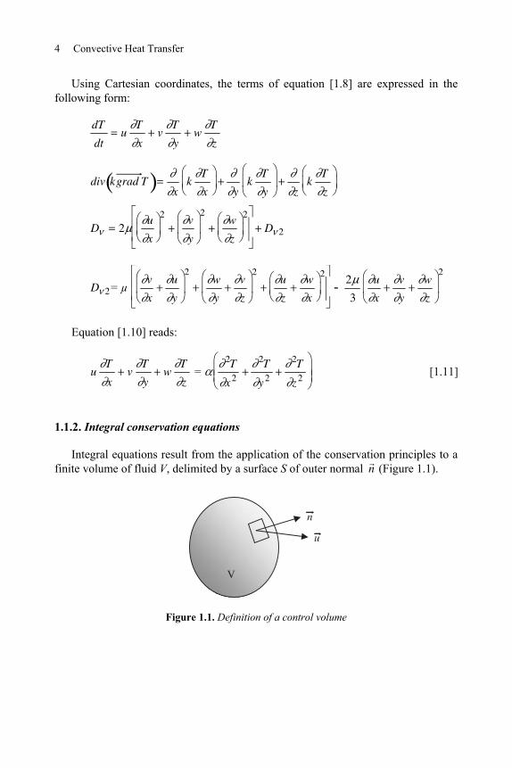
Integral equations result from the application of the conservation principles to a finite volume of fluid V, delimited by a surface S of outer normal n (Figure 1.1).
n
u
V
Figure 1.1. Definition of a control volume
Fundamental Equations, Dimensionless Numbers 5
1.1.2.1. Mass conservation
In the case of constant fluid density, the mass conservation equation may be simplified by and, in absence of sinks or sources inside the volume V, then reads:
u .n dS 0S
[1.12]
1.1.2.2. Momentum equation
The Lagrangian derivative of the fluid momentum contained in the volume V is in equilibrium with the external forces resultant R :
d
dtu dv
V
R
[1.13]
We recall that, for any scalar physical quantity:
d
dtf
vdv =
tf
vdv + f u .n
SdS [1.14]
The momentum budget may also be written as:
tu dv
V
u u .n dSS
F dvV
T n dSS
[1.15]
where F is the body force vector per unit mass inside the fluid and T n is the stress vector at a current point of the surface S. The first term of the left-hand side is zero in the case of steady flow.
1.1.2.3. Kinetic energy equation
The kinetic energy K of the fluid contained in the volume V satisfies:
e i
dKp p
dt [1.16]
with:
– K = 1
2u2dv
V;
– Pe = power of external forces (volume and surface forces);
6 Convective Heat Transfer
– Pi = power of internal forces. It can be shown that Pi may be decomposed into two parts:
Pi = Pc - D [1.17]
– Pc = mechanical power of the pressure forces during the fluid volume compression or dilatation (Pc may be positive or negative):
Pc = pd
dt
1
v
dm [1.18]
– D = viscous dissipation inside the volume V, D = V
D dv.
The viscous dissipation D is always positive and corresponds to the fluid motion irreversibilities.
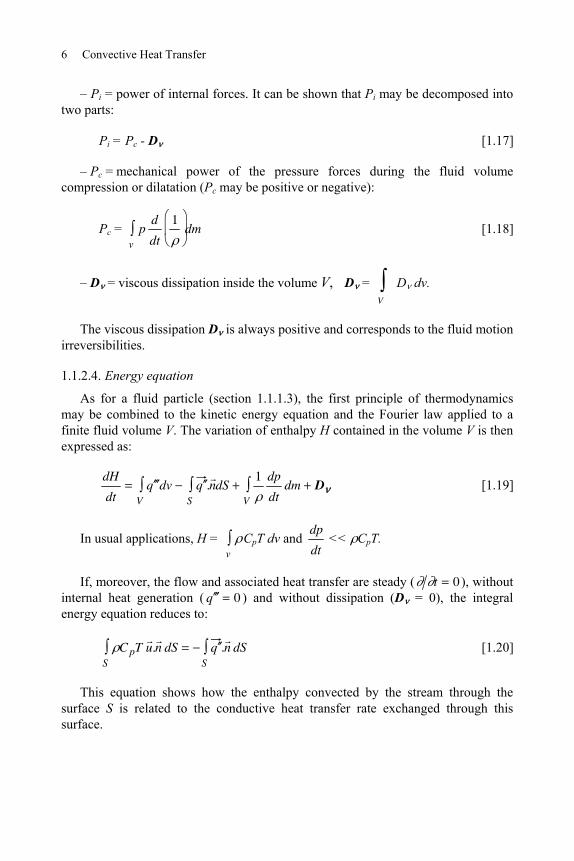
1.1.2.4. Energy equation
As for a fluid particle (section 1.1.1.3), the first principle of thermodynamics may be combined to the kinetic energy equation and the Fourier law applied to a finite fluid volume V. The variation of enthalpy H contained in the volume V is then expressed as:
dH
dtq dv
V
q .n S
dS1
V
dp
dtdm D
[1.19]
In usual applications, H = v
CpT dv and dp
dt << CpT.
If, moreover, the flow and associated heat transfer are steady ( t 0 ), without internal heat generation ( q 0 ) and without dissipation (D = 0), the integral energy equation reduces to:
C pT u .n S
dS q .n dSS
[1.20]
This equation shows how the enthalpy convected by the stream through the surface S is related to the conductive heat transfer rate exchanged through this surface.
Fundamental Equations, Dimensionless Numbers 7
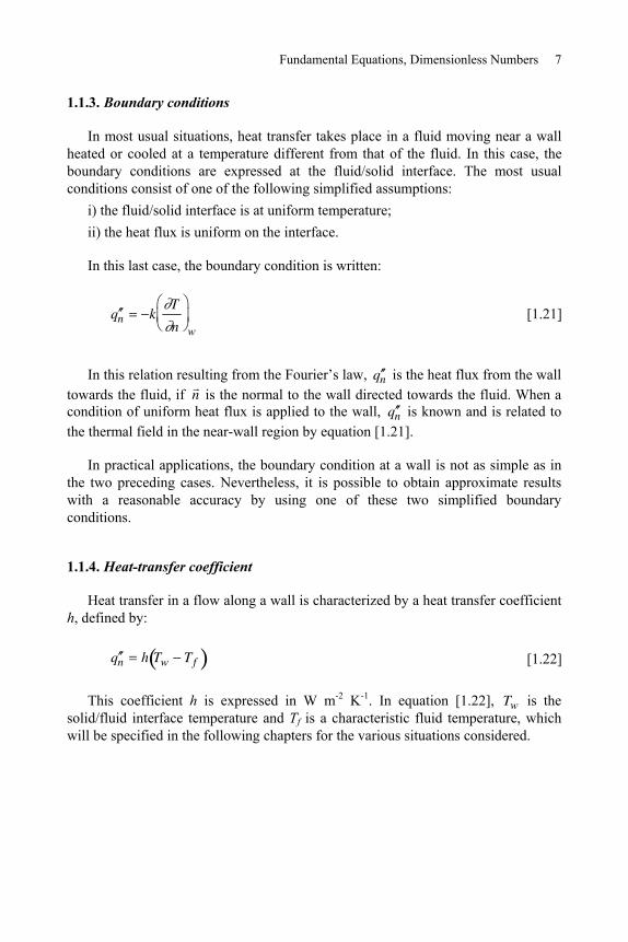
1.1.3. Boundary conditions
In most usual situations, heat transfer takes place in a fluid moving near a wall heated or cooled at a temperature different from that of the fluid. In this case, the boundary conditions are expressed at the fluid/solid interface. The most usual conditions consist of one of the following simplified assumptions:
i) the fluid/solid interface is at uniform temperature; ii) the heat flux is uniform on the interface.
In this last case, the boundary condition is written:
q n kT
n w
[1.21]
In this relation resulting from the Fourier’s law, q n is the heat flux from the wall towards the fluid, if n is the normal to the wall directed towards the fluid. When a condition of uniform heat flux is applied to the wall, q n is known and is related to the thermal field in the near-wall region by equation [1.21].
In practical applications, the boundary condition at a wall is not as simple as in the two preceding cases. Nevertheless, it is possible to obtain approximate results with a reasonable accuracy by using one of these two simplified boundary conditions.
1.1.4. Heat-transfer coefficient
Heat transfer in a flow along a wall is characterized by a heat transfer coefficient h, defined by:
q n h Tw Tf [1.22]
This coefficient h is expressed in W m-2 K-1. In equation [1.22], Tw is the solid/fluid interface temperature and Tf is a characteristic fluid temperature, which will be specified in the following chapters for the various situations considered.
8 Convective Heat Transfer
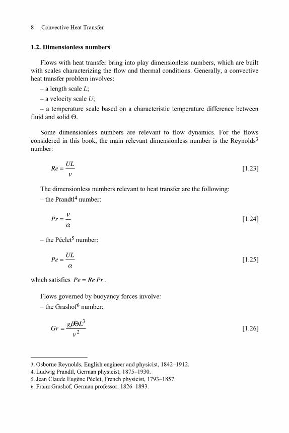
1.2. Dimensionless numbers
Flows with heat transfer bring into play dimensionless numbers, which are built with scales characterizing the flow and thermal conditions. Generally, a convective heat transfer problem involves:
– a length scale L; – a velocity scale U; – a temperature scale based on a characteristic temperature difference between
fluid and solid
Some dimensionless numbers are relevant to flow dynamics. For the flows considered in this book, the main relevant dimensionless number is the Reynolds3 number:
ReUL
[1.23]
The dimensionless numbers relevant to heat transfer are the following: – the Prandtl4 number:
Pr [1.24]
– the Péclet5 number:
PeUL
[1.25]
which satisfies Pe Re Pr .
Flows governed by buoyancy forces involve: – the Grashof6 number:
Gr =g L3
2 [1.26]
3. Osborne Reynolds, English engineer and physicist, 1842–1912. 4. Ludwig Prandtl, German physicist, 1875–1930. 5. Jean Claude Eugène Péclet, French physicist, 1793–1857. 6. Franz Grashof, German professor, 1826–1893.
Fundamental Equations, Dimensionless Numbers 9
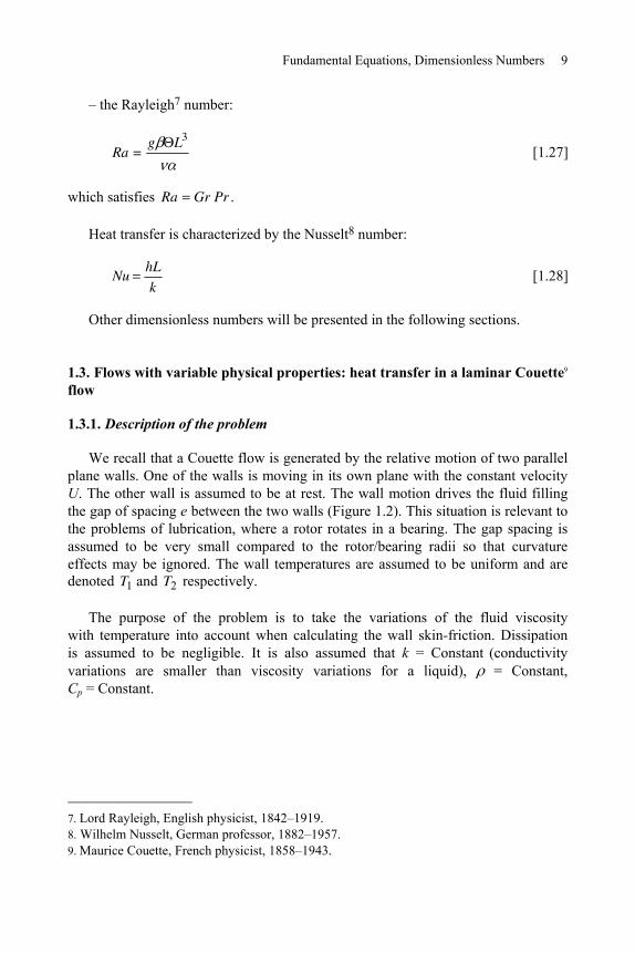
– the Rayleigh7 number:
Ra =g L3
[1.27]
which satisfies Ra Gr Pr .
Heat transfer is characterized by the Nusselt8 number:
NuhL
k [1.28]
Other dimensionless numbers will be presented in the following sections.
1.3. Flows with variable physical properties: heat transfer in a laminar Couette9 flow
1.3.1. Description of the problem
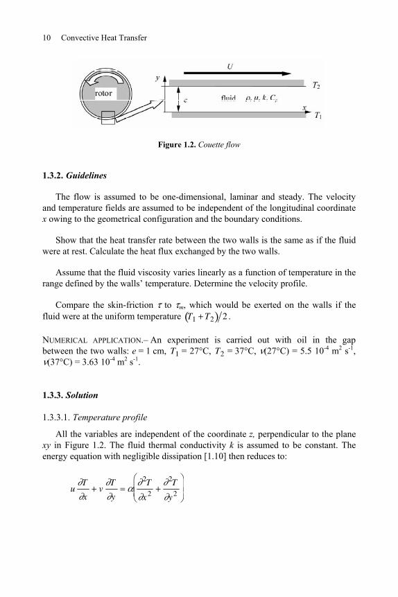
We recall that a Couette flow is generated by the relative motion of two parallel plane walls. One of the walls is moving in its own plane with the constant velocity U. The other wall is assumed to be at rest. The wall motion drives the fluid filling the gap of spacing e between the two walls (Figure 1.2). This situation is relevant to the problems of lubrication, where a rotor rotates in a bearing. The gap spacing is assumed to be very small compared to the rotor/bearing radii so that curvature effects may be ignored. The wall temperatures are assumed to be uniform and are denoted T1 and T2 respectively.
The purpose of the problem is to take the variations of the fluid viscosity with temperature into account when calculating the wall skin-friction. Dissipation is assumed to be negligible. It is also assumed that k = Constant (conductivity variations are smaller than viscosity variations for a liquid), = Constant, Cp = Constant.
7. Lord Rayleigh, English physicist, 1842–1919. 8. Wilhelm Nusselt, German professor, 1882–1957. 9. Maurice Couette, French physicist, 1858–1943.
10 Convective Heat Transfer
Figure 1.2. Couette flow
1.3.2. Guidelines
The flow is assumed to be one-dimensional, laminar and steady. The velocity and temperature fields are assumed to be independent of the longitudinal coordinate x owing to the geometrical configuration and the boundary conditions.
Show that the heat transfer rate between the two walls is the same as if the fluid were at rest. Calculate the heat flux exchanged by the two walls.
Assume that the fluid viscosity varies linearly as a function of temperature in the range defined by the walls’ temperature. Determine the velocity profile.
Compare the skin-friction to m, which would be exerted on the walls if the fluid were at the uniform temperature T1 T2 2 .
NUMERICAL APPLICATION.– An experiment is carried out with oil in the gap between the two walls: e = 1 cm, T1 = 27°C, T2 = 37°C, (27°C) = 5.5 10-4 m2 s-1,
(37°C) = 3.63 10-4 m2 s-1.
1.3.3. Solution
1.3.3.1. Temperature profile
All the variables are independent of the coordinate z, perpendicular to the plane xy in Figure 1.2. The fluid thermal conductivity k is assumed to be constant. The energy equation with negligible dissipation [1.10] then reduces to:
uT
xv
T
y
2T
x2
2T
y2
Fundamental Equations, Dimensionless Numbers 11
The flow is parallel to the walls. The velocity component v is zero. It may also be assumed that T x 0 . The energy equation therefore simplifies as:
2T
y20
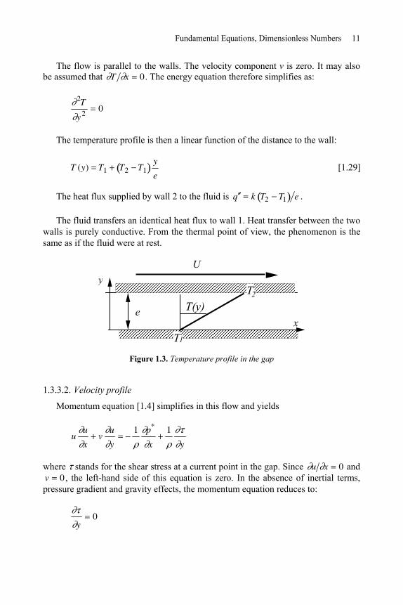
The temperature profile is then a linear function of the distance to the wall:
T (y) T1 T2 T1y
e [1.29]
The heat flux supplied by wall 2 to the fluid is q k T2 T1 e .
The fluid transfers an identical heat flux to wall 1. Heat transfer between the two walls is purely conductive. From the thermal point of view, the phenomenon is the same as if the fluid were at rest.
T1
T2
e x
y U
T(y)
Figure 1.3. Temperature profile in the gap
1.3.3.2. Velocity profile
Momentum equation [1.4] simplifies in this flow and yields
uu
xv
u
y
1 p*
x
1
y
where stands for the shear stress at a current point in the gap. Since u x 0 and v 0 , the left-hand side of this equation is zero. In the absence of inertial terms, pressure gradient and gravity effects, the momentum equation reduces to:
y0
12 Convective Heat Transfer
The shear stress is therefore constant across the gap. For a Newtonian fluid, the resulting relation is:
0 (y)du
dy [1.30]
We assume that the fluid dynamic viscosity is a linear function of temperature between T1 and T2 . The fluid viscosity at the mean temperature T1 T2 2 is denoted m. We also denote m T2 T1 m so that:
(y) m 1y
e 2
Replacing viscosity with the expression in [1.30] and introducing the dimensionless numbers:
u00e
m
, m
(T1) (T2)
(T1) (T2),
we obtain the equation satisfied by the velocity u(y):
du
dy
u0
e 1 2 y e [1.31]
The boundary conditions are the no-slip condition at the walls:
u(y 0) 0
u(y e) U
Equation [1.31] is integrated in
u( )u0
2Ln 1
2
1
where is the dimensionless distance to wall 1, y e .
The velocity scale u0 satisfies u0
U
2
Ln1
1
.
Fundamental Equations, Dimensionless Numbers 13
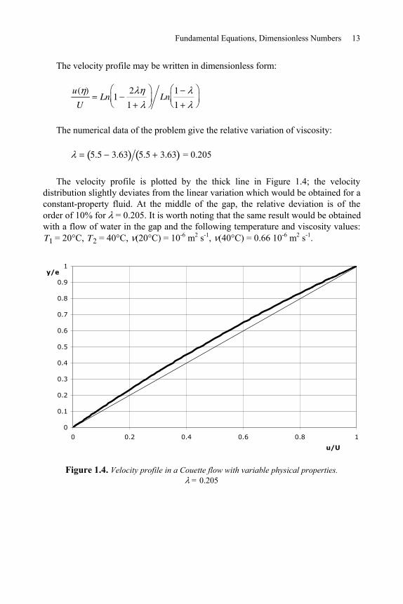
The velocity profile may be written in dimensionless form:
u( )
ULn 1
2
1Ln
1
1
The numerical data of the problem give the relative variation of viscosity:
5.5 3.63 5.5 3.63 = 0.205
The velocity profile is plotted by the thick line in Figure 1.4; the velocity distribution slightly deviates from the linear variation which would be obtained for a constant-property fluid. At the middle of the gap, the relative deviation is of the order of 10% for = 0.205. It is worth noting that the same result would be obtained with a flow of water in the gap and the following temperature and viscosity values: T1 = 20°C, T2 = 40°C, (20°C) = 10-6 m2 s-1, (40°C) = 0.66 10-6 m2 s-1.
0
0.1
0.2
0.3
0.4
0.5
0.6
0.7
0.8
0.9
1
0 0.2 0.4 0.6 0.8 1
u/U
y/e
Figure 1.4. Velocity profile in a Couette flow with variable physical properties. = 0.205
14 Convective Heat Transfer
1.3.3.3. Skin-friction
Deriving velocity with respect to y and substituting the result into equation [1.30] yields the skin-friction (constant across the gap):
0
m
2
Ln1
1
[1.32]
m is the skin-friction obtained with constant viscosity at T1 T2 2 , m m U e .
For 0.205 , equation [1.32] gives 0 m 0.984 . This result demonstrates that the skin-friction calculated by taking the viscosity variations into account is very close to the corresponding value obtained with the average viscosity at T1 T2 2 (deviation: 1.6%).
This example suggests that the computation of a flow may be carried out with reasonable accuracy using constant fluid properties at a mean temperature. It is clear that the accuracy deteriorates when the characteristic temperature variations increase in the fluid.
1.4. Flows with dissipation
1.4.1. Description of the problem
Consider the Couette flow defined in section 1.3.1 (Figure 1.2) with constant fluid properties. Determine the influence of dissipation on heat transfer between the walls and the fluid.
1.4.2. Guidelines
Calculate the dissipation function. Determine the temperature profile.
Calculate the heat flux at the two walls.
Consider a control domain delimited by the walls and apply the kinetic energy equation. Apply the integral energy equation to the same control domain.
Fundamental Equations, Dimensionless Numbers 15
1.4.3. Solution
1.4.3.1. Dissipation function
The velocity profile is linear because the fluid properties are now supposed to be constant, u( ) U .
The specific viscous dissipation is calculated using equation [1.9]. For a Couette flow, which is defined by a pure shear deformation, the only terms to be considered in the computation of D are:
dxy = dyx = 1
2
du
dy
U
2e
The dissipation function is:
D 2U
2e
2U
2e
2U 2
e2 [1.33]
1.4.3.2. Temperature profile
In energy equation [1.10], the terms of advection (left-hand side) are again zero. The dissipation function D must be added to the right-hand side in order to take into account dissipation effects. It follows that the energy equation is:
k2T
y2
U 2
e20 [1.34]
The boundary conditions are the conditions of continuity for temperature:
T (y 0) T1
T (y e) T2
A straightforward integration gives a parabolic temperature profile written in the dimensionless form:
( )T (y) T1
T2 T1
U 2
2k T2 T1
2
[1.35]
The temperature profile is therefore the superposition of a linear part (corresponding to negligible dissipation) and a parabolic part (due to dissipation).
16 Convective Heat Transfer
Equation [1.35] shows that the solution depends on the dimensionless number, called the Brinkman number:
BrU 2
k T2 T1 [1.36]
or, equivalently, on the Eckert10 number:
EcU 2
C p T2 T1 [1.37]
with Br Pr Ec .
The dimensionless temperature profile is therefore:
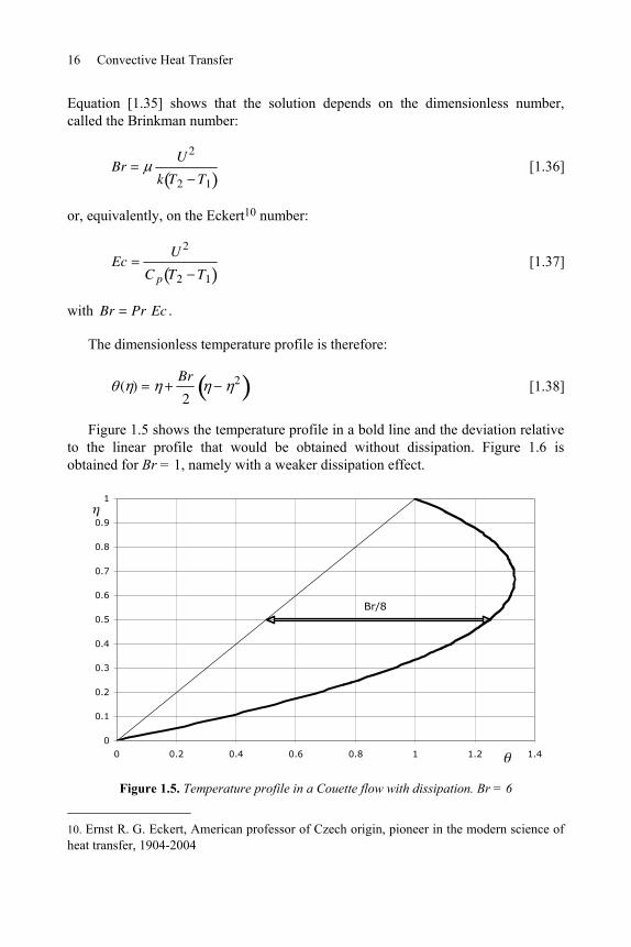
( )Br
22 [1.38]
Figure 1.5 shows the temperature profile in a bold line and the deviation relative to the linear profile that would be obtained without dissipation. Figure 1.6 is obtained for Br = 1, namely with a weaker dissipation effect.
0
0.1
0.2
0.3
0.4
0.5
0.6
0.7
0.8
0.9
1
0 0.2 0.4 0.6 0.8 1 1.2 1.4
Br/8
Figure 1.5. Temperature profile in a Couette flow with dissipation. Br = 6
10. Ernst R. G. Eckert, American professor of Czech origin, pioneer in the modern science of heat transfer, 1904-2004
Fundamental Equations, Dimensionless Numbers 17
1.4.3.3. Heat flux at the walls
The heat flux passing through a horizontal plane into Oy direction is obtained by projecting the vectorial Fourier law [1.7] upon Oy axis as:
q ( ) kT2 T1
e1
Br
21 2 [1.39]
For 0, it represents the heat flux supplied by wall 1 to the fluid. We find:
q 1 kT2 T1
e1
Br
2 [1.40]
This quantity is always negative (for T2 T1) because the heat flux due to dissipation adds to the conductive flux through the gap. In other words, wall 1 is always heated by the fluid and must be connected to a cold sink to be maintained in thermal equilibrium in the steady situation considered in this problem.
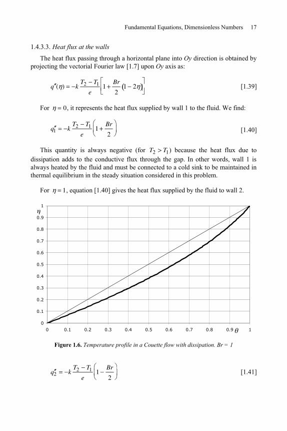
For 1, equation [1.40] gives the heat flux supplied by the fluid to wall 2.
0
0.1
0.2
0.3
0.4
0.5
0.6
0.7
0.8
0.9
1
0 0.1 0.2 0.3 0.4 0.5 0.6 0.7 0.8 0.9 1
Figure 1.6. Temperature profile in a Couette flow with dissipation. Br = 1
q 2 kT2 T1
e1
Br
2 [1.41]
18 Convective Heat Transfer
For wall 2, the dissipation effect is opposite to heat conduction from wall 2 towards wall 1, so that q 2 can be positive or negative, depending on the value of Br.
When Br < 2, q 2 < 0. The fluid is heated by wall 2 (Figure 1.6).
When Br > 2, q 2 > 0. This is the example shown in Figure 1.5. It is necessary to remove the heat flux q 2 (positive) from wall 2 to maintain the system in thermal equilibrium.
1.4.3.4. Global approach
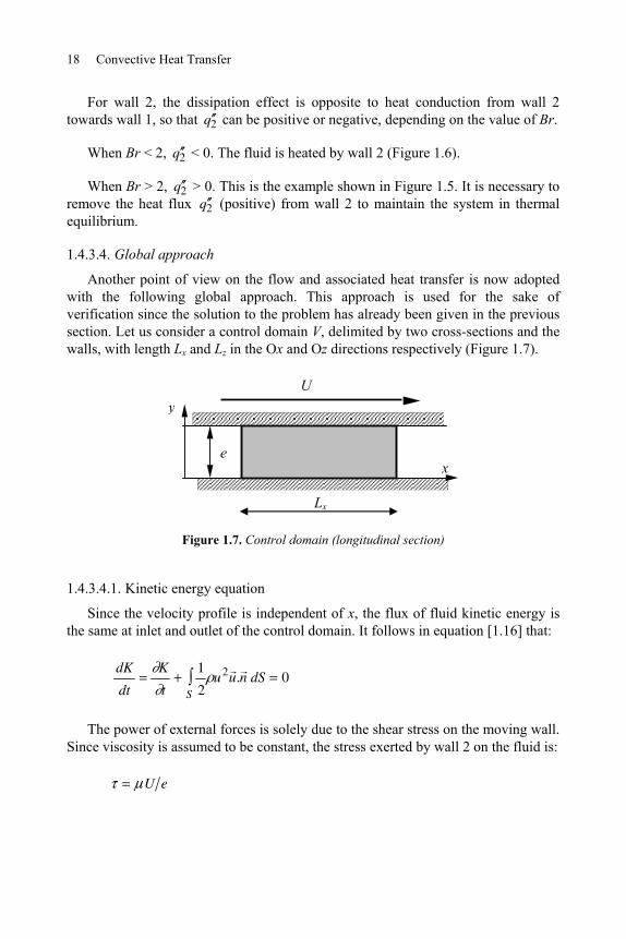
Another point of view on the flow and associated heat transfer is now adopted with the following global approach. This approach is used for the sake of verification since the solution to the problem has already been given in the previous section. Let us consider a control domain V, delimited by two cross-sections and the walls, with length Lx and Lz in the Ox and Oz directions respectively (Figure 1.7).
e x
y U
Lx
Figure 1.7. Control domain (longitudinal section)
1.4.3.4.1. Kinetic energy equation
Since the velocity profile is independent of x, the flux of fluid kinetic energy is the same at inlet and outlet of the control domain. It follows in equation [1.16] that:
dK
dt
K
t
1
2S
u2u .n dS 0
The power of external forces is solely due to the shear stress on the moving wall. Since viscosity is assumed to be constant, the stress exerted by wall 2 on the fluid is:
U e
Fundamental Equations, Dimensionless Numbers 19
The corresponding power is
Pe ULxLzU 2
eSlat [1.42]
where Slat denotes the lateral surface of the control volume ( Slat LxLz ).
The power of internal forces is only due to dissipation and equation [1.16] reduces to:
Pe = D
In other words, the mechanical power supplied to the fluid by the moving wall is entirely dissipated in the gap.
The viscous dissipation is calculated by:
D = D dv =V
Slatdu
dy0e
2
dyU 2
e2e Slat
[1.43]
Comparison of equations [1.42] and [1.43] shows that the kinetic energy budget is satisfied.
1.4.3.4.2. Energy equation
Since the velocity and temperature profiles are independent of x, the flux of enthalpy is the same at inlet and outlet of the control domain. It follows that dH dt 0 in equation [1.19]. For the same reason, the power expended in the compression or dilation of the fluid particles is zero. It follows that:
- q .n S
dS + D = 0 [1.44]
The heat dissipated in the gap is entirely evacuated by the walls. It is worth examining the role played by the two walls in the thermal equilibrium of the system.
The normal n is directed towards the exterior of the control volume. On wall 1, n y . The contribution to the integral in [1.44] is the heat transfer rate supplied to the flow. This quantity is always negative, as was seen in section 1.4.3.3 (wall 1 always evacuates heat towards the environment):
- q".n S1
dS = q 1Slat
20 Convective Heat Transfer
On wall 2, n y , so that:
- q .n S2
dS = - q 2Slat
On wall 2, the heat rate supplied to the flow may be positive or negative, as was seen in section 1.4.3.3. If dissipation is weak (Br < 2, q 2 < 0), heat transfer is mainly governed by conduction so that wall 2 supplies heat to the fluid (Figure 1.6).
Using [1.40] and [1.41], we check that:
q 1 q 2 Slat kBr
eSlat
U2
eSlat
[1.45]
Comparing [1.43] and [1.45], we check that the energy equation is satisfied.
1.5. Cooling of a sphere by a gas flow
1.5.1. Description of the problem
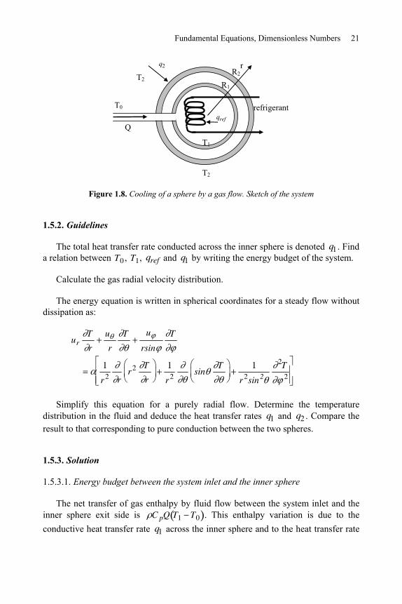
A system is composed of two concentric porous spheres, S1 and S2, of radii R1 and R2 respectively. The sphere S2 is heated at the total heat transfer rate q2 (electrical heating, radiation, etc.). A stream of gas is cooled by a refrigerant and then flows radially across the inner sphere S1 at flow rate Q (Figure 1.8). The gas flows further downstream across the sphere S2 toward the environment at the same temperature as S2. The sphere S2 is then maintained in equilibrium at temperature T2 . The sphere S1 is assumed to be also in thermal equilibrium at temperature T1 under the influence of conduction at its inner and outer sides.
The system is operated in steady regime. The gas temperature at the system inlet is denoted T0 . Calculate the total heat transfer rate of refrigeration qref that it is necessary to remove from the gas stream in order to maintain the inner sphere at temperature T1 when the external sphere is maintained at temperature T2 ( T1). The gas flow is assumed to be radial and laminar. Heat losses are ignored in the inlet duct. The gas properties are density , specific heat at constant temperature C p and thermal conductivity k.
Fundamental Equations, Dimensionless Numbers 21
T1
T2
R1
R2r
T0
Q
refrigerant
q2
T2
qref
Figure 1.8. Cooling of a sphere by a gas flow. Sketch of the system
1.5.2. Guidelines
The total heat transfer rate conducted across the inner sphere is denoted q1 . Find a relation between T0 , T1, qref and q1 by writing the energy budget of the system.
Calculate the gas radial velocity distribution.
The energy equation is written in spherical coordinates for a steady flow without dissipation as:
urT
r
u
r
T u
rsin
T
1
r 2 rr2 T
r
1
r2sin
T 1
r2sin2
2T2
Simplify this equation for a purely radial flow. Determine the temperature distribution in the fluid and deduce the heat transfer rates q1 and q2 . Compare the result to that corresponding to pure conduction between the two spheres.
1.5.3. Solution
1.5.3.1. Energy budget between the system inlet and the inner sphere
The net transfer of gas enthalpy by fluid flow between the system inlet and the inner sphere exit side is C pQ T1 T0 . This enthalpy variation is due to the conductive heat transfer rate q1 across the inner sphere and to the heat transfer rate
22 Convective Heat Transfer
qref removed by the refrigerant. q1 is counted positively in the direction - r in accordance with intuition (heat is transferred from S2 to S1). qref is counted positively from the gas to the refrigerant. The energy budget then reads:
C pQ T1 T0 q1 qref [1.46]
Several operating modes are possible. For example, the system may be fed in gas at temperature T1. In this case, the heat transfer rate necessary to maintain the sphere S1 at temperature T1 is simply qref q1. The gas is first cooled by the refrigerant and then heated by conduction near the wall of sphere S1. This issue will be detailed thereafter.
It is also possible to operate the system with a gas inlet temperature different from T1. In this case, the heat transfer rate removed by the refrigerant is:
qref q1 C pQ T0 T1
When compared to the previous case, the refrigerant must remove the additional heat transfer rate C pQ T0 T1 , if T0 T1. Conversely, the cooling rate is decreased if T0 T1.
1.5.3.2. Radial velocity
The gas flow rate is constant in the whole system and is therefore the same across any sphere of radius r. The radial velocity distribution is then obtained as:
ur rQ
4 r2 [1.47]
1.5.3.3. Temperature distribution between the two spheres
The temperature distribution between the two spheres is governed by the energy equation, which is simplified in this case by using u u 0 as:
urT
r r 2 rr2 T
r [1.48]
Fundamental Equations, Dimensionless Numbers 23
Replacing ur with expression [1.47] and simplifying, the energy equation reads
Pe 2
[1.49]
where the dimensionless quantities PeQ
4 R1, r R1 and
T T1
T2 T1 have
been introduced. The ratio of the sphere radii is denoted R* R2 R1 .
The Péclet number is Pe U1R1 , where U1 is the gas velocity at the position of sphere S1.
It is worth noting that equation [1.48] results from the balance between radial advection (left-hand side) and radial conduction (right-hand side). In other words, the velocity and heat flux vectors are aligned. This is an unusual situation in convective heat transfer since, in fact, these two vectors are nearly perpendicular in most cases, as will be seen in the following chapters; generally, conduction operates mainly in the direction perpendicular to the flow.
The temperature field satisfies the continuity boundary condition. We assume that the two porous spheres are in thermal equilibrium; in other words, the gas and the porous matrix in each sphere are at the same temperature. Using dimensionless variables, the boundary conditions are:
1 0
R* 1
Equation [1.49] is integrated in a first step
Pe 2 A
[1.50]
whose general solution is A
PeBe Pe .
The two constants of integration A and B are calculated by taking the two boundary conditions into account. The temperature distribution is finally obtained as:
1 ePe 1 1
1 ePe 1 1 R*
[1.51]
24 Convective Heat Transfer
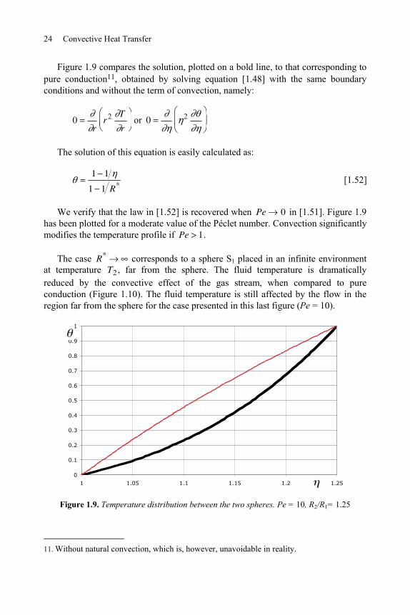
Figure 1.9 compares the solution, plotted on a bold line, to that corresponding to pure conduction11, obtained by solving equation [1.48] with the same boundary conditions and without the term of convection, namely:
0r
r2 T
r or 0 2
The solution of this equation is easily calculated as:
1 1
1 1 R*
[1.52]
We verify that the law in [1.52] is recovered when Pe 0 in [1.51]. Figure 1.9 has been plotted for a moderate value of the Péclet number. Convection significantly modifies the temperature profile if Pe 1.
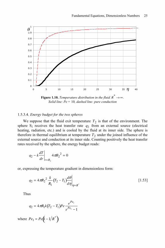
The case R* corresponds to a sphere S1 placed in an infinite environment at temperature T2 , far from the sphere. The fluid temperature is dramatically reduced by the convective effect of the gas stream, when compared to pure conduction (Figure 1.10). The fluid temperature is still affected by the flow in the region far from the sphere for the case presented in this last figure (Pe = 10).
0
0.1
0.2
0.3
0.4
0.5
0.6
0.7
0.8
0.9
1
1 1.05 1.1 1.15 1.2 1.25
Figure 1.9. Temperature distribution between the two spheres. Pe = 10, R2/R1= 1.25
11. Without natural convection, which is, however, unavoidable in reality.
Fundamental Equations, Dimensionless Numbers 25
0
0.1
0.2
0.3
0.4
0.5
0.6
0.7
0.8
0.9
1
0 5 10 15 20 25 30 35 40
Figure 1.10. Temperature distribution in the fluid. R* . Solid line: Pe = 10, dashed line: pure conduction
1.5.3.4. Energy budget for the two spheres
We suppose that the fluid exit temperature T2 is that of the environment. The sphere S2 receives the heat transfer rate q2 from an external source (electrical heating, radiation, etc.) and is cooled by the fluid at its inner side. The sphere is therefore in thermal equilibrium at temperature T2 under the joined influence of the external source and conduction at its inner side. Counting positively the heat transfer rates received by the sphere, the energy budget reads:
q2 kdT
dr r R2
4 R22 0
or, expressing the temperature gradient in dimensionless form:
q2 4 R22 k
R1T2 T1
d
d R*
[1.53]
Thus
q2 4 R1k T2 T1 PeePe1
ePe1 1
where Pe1 Pe 1 1 R*
26 Convective Heat Transfer
The same calculation is performed for pure conduction ( Pe 0 ) and gives the same result as [1.53] with, however, the dimensionless temperature gradient resulting from [1.52]. We then calculate the heat transfer rate removed by the fluid normalized by the pure conduction heat transfer rate as:
q2* q2 conv.
q2 cond.
d dR*
conv.
d dR*
cond.
[1.54]
The result is:
q2* Pe1
ePe1
ePe1 1 [1.55]
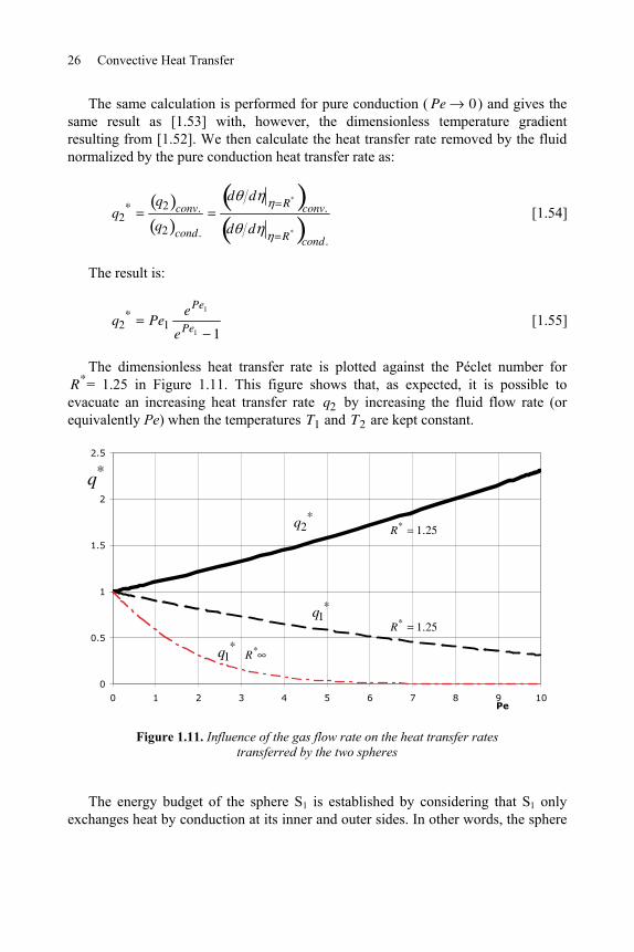
The dimensionless heat transfer rate is plotted against the Péclet number for R*= 1.25 in Figure 1.11. This figure shows that, as expected, it is possible to evacuate an increasing heat transfer rate q2 by increasing the fluid flow rate (or equivalently Pe) when the temperatures T1 and T2 are kept constant.
0
0.5
1
1.5
2
2.5
0 1 2 3 4 5 6 7 8 9 10Pe
R*
q2*
q1*
q1*
R* 1.25
R* 1.25
q*
Figure 1.11. Influence of the gas flow rate on the heat transfer rates transferred by the two spheres
The energy budget of the sphere S1 is established by considering that S1 only exchanges heat by conduction at its inner and outer sides. In other words, the sphere
Fundamental Equations, Dimensionless Numbers 27
is “transparent” from the thermal point of view. The heat transfer rate q1 , (counted positively in the direction - r ) across the sphere is given by
q1 kdT
dr r R1
4 R12 = 4 R1
2 k
R1T2 T1
d
d 1
or q1 4 R1k T2 T1Pe
ePe1 1.
As for sphere 2, it is instructive to normalize q1 with the heat transfer rate corresponding to pure conduction as:
q1*
d d 1 conv.
d d 1 cond.
Pe1
ePe1 1
[1.56]
The result is plotted by the black dashed line in Figure 1.11. It may be noted that the heat transfer rate q1 decreases when the Péclet number is increased. The heat transfer rate qref removed by the refrigerant follows the same trend (equation [1.46]).
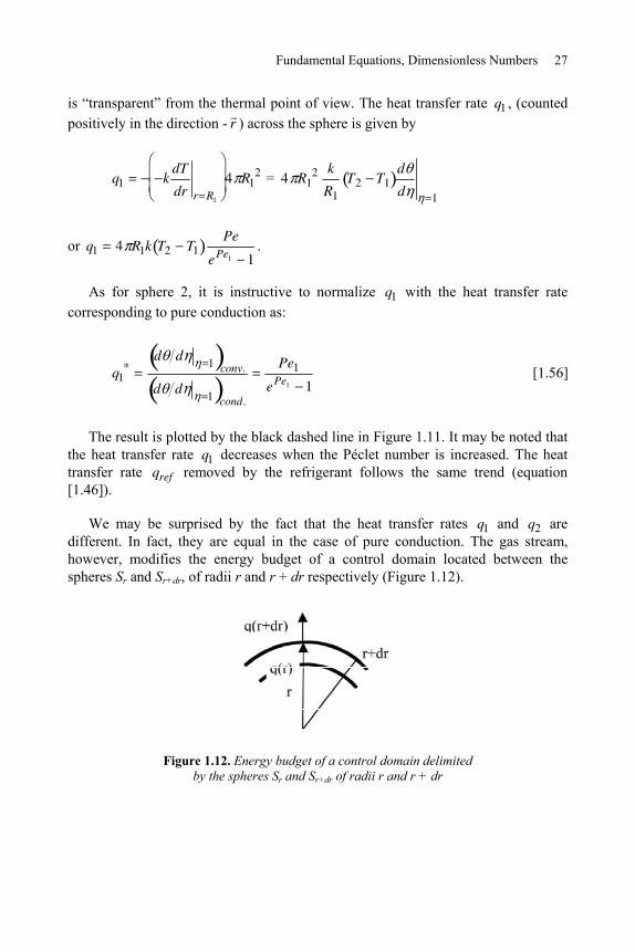
We may be surprised by the fact that the heat transfer rates q1 and q2 are different. In fact, they are equal in the case of pure conduction. The gas stream, however, modifies the energy budget of a control domain located between the spheres Sr and Sr+dr, of radii r and r + dr respectively (Figure 1.12).
Figure 1.12. Energy budget of a control domain delimited by the spheres Sr and Sr+dr of radii r and r + dr
28 Convective Heat Transfer
Equation [1.20] applied to this control domain shows that
C pT u .n Sr Sr dr
dS C pQT r C pQT r dr = C pQdT
drdr
since the temperature is uniform on each sphere;
q .n dSS
q r dr q rdq
drdr
since n is the outer normal to a surface and q r is counted positively in the direction r .
Finally, the energy budget reads:
C pQdT
drdq [1.57]
Integrating:
C pQT r q r Cte [1.58]
The heat transfer rate q r therefore varies between the two spheres S1 and S2.
Equation [1.58], written for the two spheres, gives
C pQT1 q1 C pQT2 q2
since q1 and q2 are counted positively in the direction - r ( q r R1 q1, q r R2 q2 ). The heat transfer rates then verify:
q2 q1 C pQ T2 T1 [1.59]
It may be noticed that equation [1.58] is also obtained by integrating energy equation [1.48] with respect to r (let us emphasize that the integral equations are not independent of the local equations).
Fundamental Equations, Dimensionless Numbers 29
In fact, replacing q r kdT
dr r
4 r2 in [1.58], we obtain:
C pQT r kdT
dr r
4 r 2 C te
When dimensionless variables are used, equation [1.50] is recovered.
In the example when R* (the sphere S1 is placed in an infinite space), the conductive heat transfer rate q1
* is obtained by replacing Pe1 by Pe in [1.56], hence:
q1* Pe
ePe 1 [1.60]
The result is plotted on the long- and short-dashed lines in Figure 1.11, which shows that the heat transfer rate across the sphere S1 rapidly decreases when the Péclet number is increased.
These results demonstrate the efficiency of convection compared to conduction when the sphere S1 must be maintained at given temperature for fixed external temperature. Due to the gas stream, the sphere S1 is in a way protected by fluid at the same temperature T1 (Figure 1.10).

This page intentionally left blank
Chapter 2
Laminar Fully Developed Forced Convection in Ducts
2.1. Hydrodynamics
Heat transfer is often present in duct flows. This is the case, for example, in shell-and-tube or in tube bank heat exchangers. Typically, a fluid circulates inside tubes while another fluid flows at a different temperature outside the tubes. Heat is transferred by convection between each fluid and adjacent walls and by conduction across the walls separating the two fluids. This chapter is devoted to the part of heat transfer that takes place at the inner surface of the tube walls. The discussion is restricted to laminar flows.
2.1.1. Characteristic parameters
A round tube is characterized by its diameter D (Figure 2.1). For a duct cross-section of a different shape it is common to use the hydraulic diameter Dh instead of D in hydraulic and thermal correlations
Dh4S
P [2.1]
where S is the cross-section area and P the wetted perimeter.
The flow is characterized by the bulk velocity. When the flow rate is Q, the mean or bulk velocity is calculated by:
32 Convective Heat Transfer
UmQ
S [2.2]
The flow regime is characterized by the Reynolds number, defined with the kinematic viscosity at a mean temperature in the duct:
ReUmDh [2.3]
This chapter is restricted to moderate values of the Reynolds number. Although not an absolute criteria, it is generally accepted that the flow is laminar for Re about 2,400.
2.1.2. Flow regions
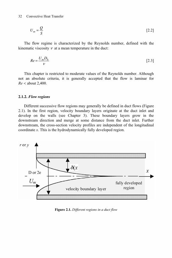
Different successive flow regions may generally be defined in duct flows (Figure 2.1). In the first region, velocity boundary layers originate at the duct inlet and develop on the walls (see Chapter 3). These boundary layers grow in the downstream direction and merge at some distance from the duct inlet. Further downstream, the cross-section velocity profiles are independent of the longitudinal coordinate x. This is the hydrodynamically fully developed region.
Figure 2.1. Different regions in a duct flow
Laminar Fully Developed Forced Convection in Ducts 33
It is generally accepted that the laminar flow regime is fully developed for:
x
D
1
Re0.04 [2.4]
In the fully developed laminar flow region, the velocity profile is:
u( )
Um
A 1 2 [2.5]
with:
– r
D 2 and A 2 for a round tube;
– y e ( y 0 on the symmetry-axis of the duct) and A 3 2 for a rectangular duct of width 2e and a very high aspect ratio (span length Lz e ) or for a flow between infinite parallel plates.
In the fully developed region, the modified pressure p* (constant in a duct cross-section) decreases linearly along the duct. The head loss coefficient is defined with the pressure drop p* between two cross-sections separated by the length L as:
p* 1
2Um
2 L
Dh
[2.6]
is inversely proportional to the Reynolds number in the laminar regime:
B
Re [2.7]
with: – B = 64 for a round tube; – B = 96 for a flow between parallel plates.
2.2. Heat transfer
2.2.1. Thermal boundary conditions
Several thermal boundary conditions are found in practical applications. As was seen in Chapter 1 (section 1.2.3), the first distinction is between uniform wall
34 Convective Heat Transfer
temperature and uniform wall heat flux heating. On the other hand, heating may start at the duct inlet or in the hydrodynamically fully developed region. In both cases, thermal boundary layers develop on the duct walls and merge at some distance from the start of heating. Further downstream, the thermal field is fully developed in the duct. The definition of this thermally fully developed region will be given thereafter.
2.2.2. Bulk temperature
It is useful to define a mean temperature in a duct cross-section. The bulk temperature is defined by:
Tm x1
C pQC pT udSS [2.8]
This is the characteristic fluid temperature used in heat transfer correlations. In the integral of equation [2.8], u and T are respectively the velocity and temperature at a current point of the cross-section S. We recall that Q is the flow rate in the duct.
2.2.3. Heat-transfer coefficient
The local heat-transfer coefficient h(x) is defined by:
q (x) h(x) Tw(x) Tm (x) [2.9]
where q (x) is the heat flux supplied by the wall to the fluid and Tw(x) is the wall temperature (it is assumed here that these two quantities are uniform on the walls of a duct cross-section; otherwise, they are averaged on the duct cross-section periphery).
The local Nusselt number is deduced from the previous definition as:
Nu(x)h(x)Dh
k f
[2.10]
2.2.4. Fully developed thermal region
The above-mentioned fully developed thermal region is specified in this section. It is defined as the region where the shape of the cross-section temperature profile is
Laminar Fully Developed Forced Convection in Ducts 35
independent of the longitudinal coordinate x. The temperature distribution is then written in dimensionless form as:
Tw(x) T (x, r)
Tw(x) Tm (x)( ) [2.11]
The previously defined variable represents the dimensionless coordinate (r or y) in a cross-section. It is easily verified that the heat-transfer coefficient and the Nusselt number are also independent of x in this region. The entrance region characteristic length Lt depends on the thermal boundary conditions and on the Prandtl number, since the boundary layers developing in the entrance region depend on these parameters. When the velocity and thermal boundary layers develop simultaneously in the laminar regime, the length Lt is estimated by:
1 0 04.tLD RePr
[2.12]
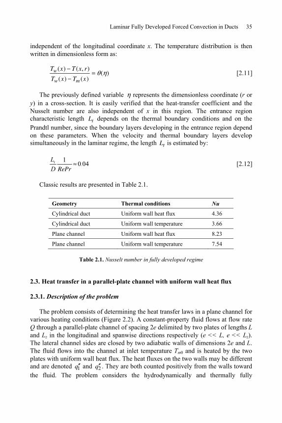
Classic results are presented in Table 2.1.
Geometry Thermal conditions Nu
Cylindrical duct Uniform wall heat flux 4.36
Cylindrical duct Uniform wall temperature 3.66
Plane channel Uniform wall heat flux 8.23
Plane channel Uniform wall temperature 7.54
Table 2.1. Nusselt number in fully developed regime
2.3. Heat transfer in a parallel-plate channel with uniform wall heat flux
2.3.1. Description of the problem
The problem consists of determining the heat transfer laws in a plane channel for various heating conditions (Figure 2.2). A constant-property fluid flows at flow rate Q through a parallel-plate channel of spacing 2e delimited by two plates of lengths L and Lz in the longitudinal and spanwise directions respectively (e << L, e << Lz). The lateral channel sides are closed by two adiabatic walls of dimensions 2e and L. The fluid flows into the channel at inlet temperature Tm0 and is heated by the two plates with uniform wall heat flux. The heat fluxes on the two walls may be different and are denoted q 1 and q 2 . They are both counted positively from the walls toward the fluid. The problem considers the hydrodynamically and thermally fully
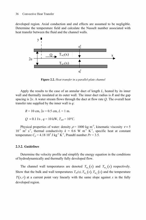
36 Convective Heat Transfer
developed region. Axial conduction and end effects are assumed to be negligible. Determine the temperature field and calculate the Nusselt number associated with heat transfer between the fluid and the channel walls.
x
y
Tw2(x)
q 2
q 1
2e Tw1(x)
Q
Figure 2.2. Heat transfer in a parallel-plate channel
Apply the results to the case of an annular duct of length L, heated by its inner wall and thermally insulated at its outer wall. The inner duct radius is R and the gap spacing is 2e. A water stream flows through the duct at flow rate Q. The overall heat transfer rate supplied by the inner wall is q:
R = 10 cm, 2e = 0.5 cm, L = 1 m.
Q l/s q = 10 kW, Tm0 = 10°C.
Physical properties of water: density = 1000 kg m-3, kinematic viscosity 5 10-7 m2 s-1, thermal conductivity k = 0.6 W m-1 K-1, specific heat at constant temperature Cp = 4.18 103 J kg-1 K-1, Prandtl number Pr = 3.5.
2.3.2. Guidelines
Determine the velocity profile and simplify the energy equation in the conditions of hydrodynamically and thermally fully developed flow.
The channel wall temperatures are denoted Tw1x and Tw2
x respectively. Show that the bulk and wall temperatures Tm(x), Tw1
x , Tw2x and the temperature
T x, r at a current point vary linearly with the same slope against x in the fully developed region.
Laminar Fully Developed Forced Convection in Ducts 37
Solve the energy equation and determine the temperature profile in a duct cross-section T y,Tw1
, q 1, q 2 , e, k . Deduce the temperature of the opposite wall
Tw2Tw1
, q 1, q 2 , e, k .
Calculate the bulk temperature Tm Tw1, q 1, q 2 , e, k . Deduce the Nusselt number.
Examine the different cases (symmetric heating, wall 2 insulated, opposite heat fluxes on the two walls).
2.3.3. Solution
2.3.3.1. Velocity profile
In laminar flow regime ( u(y) , v 0), the Navier-Stokes equations reduce for a two-dimensional flow to:
0dp
dx
d 2u
dy2
p
y
and are solved by taking into account the no-slip condition on the channel walls ( u 0 for y e ). The velocity profile [2.5] obtained is:
u( )
Um
3
21 2 [2.13]
with y
e.
2.3.3.2. Temperature profile
Energy equation [1.11] is simplified as:
u(y)T
x
2T
y2 [2.14]
It is shown below that T x is constant with respect to x.
38 Convective Heat Transfer
Actually, energy budget [1.20] yields for a slide of length dx delimited by the channel cross-section:
C pUm 2eLzdTm
dxdx q 1 q 2 Lzdx [2.15]
when axial conduction is negligible. Hence, the longitudinal temperature gradient is:
dTm
dx
q 1 q 2C pUm 2e
[2.16]
or introducing the dimensionless abscissa x 2e :
dTm
d
q 1 q 2C pUm
a [2.17]
where the constant a has the dimension of temperature.
On the other hand, the heat flux q 1 is related to the temperature gradient normal to wall 1 by:
q 1 kT
y y e
[2.18]
For the thermally fully developed regime, equation [2.11] is written for a plane channel as
Tw(x) T (x, y)
Tw(x) Tm (x)( ) [2.19]
where the function ( ) represents the x-independent shape of the temperature profile and Tw x is a function of x to be determined. Replacing the expression T(x, y) deduced from [2.19] in equation [2.18], the wall heat flux becomes:
q 1 kTw (x) Tm (x)
e' ( 1) [2.20]
which completely determines the wall temperature Tw x as a function of Tm x , when ( ) is known and shows that Tw x varies linearly against x with the same slope as Tm x . Equation [2.19], written for 1, shows that Tw1
x and Tw2x
Laminar Fully Developed Forced Convection in Ducts 39
also vary linearly against x like Tm x . The same reasoning applies to the current temperature T(x, r). Using the dimensionless variable , the temperature gradient is written:
T ,a
Energy equation [2.14] then becomes:
3
2Um 1 2 a
2e e2
2T2
or, denoting Pe Um 4e :
3
16aPe 1 2
2T2
[2.21]
This equation is integrated in:
T ( , )3
16aPe
2
2
4
12A( ) B( )
The function A is determined with the boundary condition [2.18] and the corresponding one on wall 2, namely:
q 12k
e
3
16aPe
3
3A
1
q 22k
e
3
16aPe
3
3A
1
Subtracting the two relations, we find that A is a constant:
Aq 2 q 1
4k2e [2.22]
40 Convective Heat Transfer
Summing the two relations, result [2.17] is obtained ( a4
Pe
q 1 q 2k
e ). The
temperature at a current point is then written as:
T ,3
8
q 1 q 2k
e 24
6
q 2 q 12k
e B( )
The function B may be related to the temperature of wall 1 ( 1):
B Tw15
16
q 1 q 2k
eq 2 q 1
2ke
Eliminating B, the temperature becomes:
T Tw1q 1 q 2
k
e
83 2
4
6
5
2
q 2 q 12k
e 1
and the temperature of wall 2 ( 1) is given by:
Tw2 Tw1q 2 q 1
ke [2.23]
2.3.3.3. Bulk temperature
The bulk temperature is obtained by integrating the temperature weighted by the local velocity (equation [2.8]):
Tm x1
C pQC pT x, u dSS
or, equivalently, since Tw1 is independent of :
Tw1 x Tm x1
STw1 x T x,
u
Um
dSS
Tw1 x Tm x
1
2
q 1 q 2k
e
83 2
4
6
5
2
q 2 q 12k
e 13
21 2 d1
1
Laminar Fully Developed Forced Convection in Ducts 41
Finally, we find that:
Tw1 x Tm xe
k
17
70q 1 q 2
1
2q 1 q 2 [2.24]
2.3.3.4. Nusselt number
The Nusselt number may be based on q 1 or q 2 , while the characteristic dimension is the hydraulic diameter (Dh = 4e):
Nu1q 1
kTw1 Tm
4e
Nu2q 2
kTw2 Tm
4e
Using [2.24], we find that:
Nu1140
26 9q 2q 1
[2.25]
2.3.3.5. Study of the different cases
2.3.3.5.1. Symmetric heating ( q 1 = q 2 )
The two channel walls are obviously at same temperature. The temperature difference between the wall and the fluid ([2.23]) is:
Tw1(x) Tm x17eq 135k
[2.26]
The fluid temperature profile is symmetric with respect to the symmetry-axis of the channel:
T x, Tw1 xq 1k
e
43 2
4
6
5
2
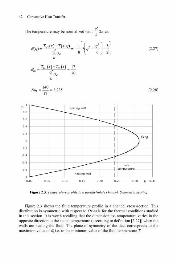
42 Convective Heat Transfer
The temperature may be normalized with q 1k
2e as:
Tw1 x T x,q 1k
2e
1
83 2
4
6
5
2 [2.27]
mTw1 x Tm x
q 1k
2e
17
70
Nu1140
178.235 [2.28]
-1
-0.8
-0.6
-0.4
-0.2
0
0.2
0.4
0.6
0.8
1
0.00 0.05 0.10 0.15 0.20 0.25 0.30 0.35
heating wall
heating wall
bulk temperature
Figure 2.3. Temperature profile in a parallel-plate channel. Symmetric heating
Figure 2.3 shows the fluid temperature profile in a channel cross-section. This distribution is symmetric with respect to Ox-axis for the thermal conditions studied in this section. It is worth recalling that the dimensionless temperature varies in the opposite direction to the actual temperature (according to definition [2.27]) when the walls are heating the fluid. The plane of symmetry of the duct corresponds to the maximum value of , i.e. to the minimum value of the fluid temperature T.
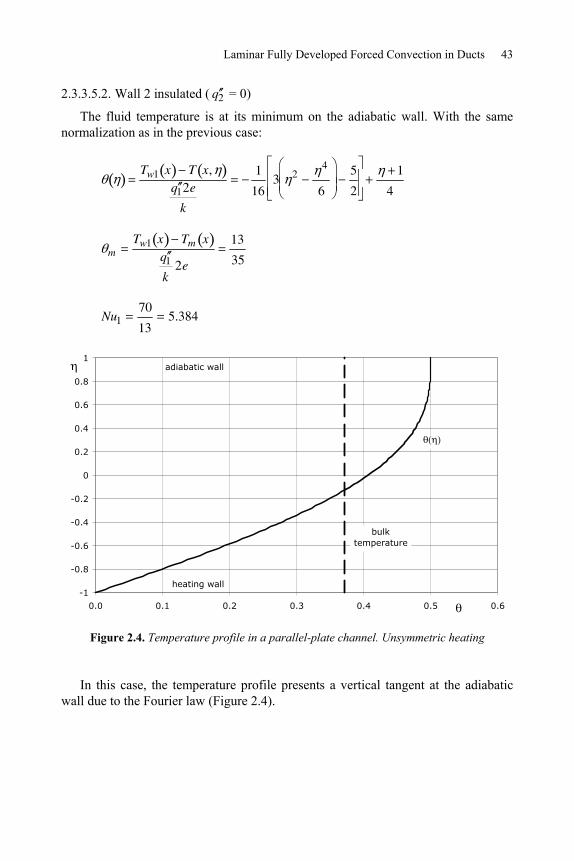
Laminar Fully Developed Forced Convection in Ducts 43
2.3.3.5.2. Wall 2 insulated ( q 2 = 0)
The fluid temperature is at its minimum on the adiabatic wall. With the same normalization as in the previous case:
Tw1 x T x,q 12e
k
1
163 2
4
6
5
2
1
4
mTw1 x Tm x
q 1k
2e
13
35
Nu170
135.384
-1
-0.8
-0.6
-0.4
-0.2
0
0.2
0.4
0.6
0.8
1
0.0 0.1 0.2 0.3 0.4 0.5 0.6
bulk temperature
heating wall
adiabatic wall
Figure 2.4. Temperature profile in a parallel-plate channel. Unsymmetric heating
In this case, the temperature profile presents a vertical tangent at the adiabatic wall due to the Fourier law (Figure 2.4).
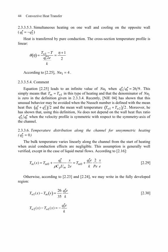
44 Convective Heat Transfer
2.3.3.5.3. Simultaneous heating on one wall and cooling on the opposite wall ( q 1 q 2 )
Heat is transferred by pure conduction. The cross-section temperature profile is linear:
Tw1 Tq 12e
k
1
2
According to [2.25], Nu1 4 .
2.3.3.5.4. Comment
Equation [2.25] leads to an infinite value of Nu1 when q 2 q 1 26 9 . This simply means that Tm Tw1 in this type of heating and that the denominator of Nu1 is zero in the definition given in 2.3.3.4. Recently, [NIE 04] has shown that this unusual behavior may be avoided when the Nusselt number is defined with the mean heat flux q 1 q 2 2 and the mean wall temperature Tw1 Tw2 2 . Moreover, he has shown that, using this definition, Nu does not depend on the wall heat flux ratio q 2 q 1 when the velocity profile is symmetric with respect to the symmetry-axis of the channel.
2.3.3.6. Temperature distribution along the channel for unsymmetric heating ( q 2 0 )
The bulk temperature varies linearly along the channel from the start of heating when axial conduction effects are negligible. This assumption is generally well verified, except in the case of liquid metal flows. According to [2.16]:
Tm (x) Tm0q 1
C pUm
x
2eTm0
q 1e
k
2
Pe
x
e [2.29]
Otherwise, according to [2.23] and [2.24], we may write in the fully developed region:
Tw1(x) Tm x26
35
q 1e
k [2.30]
Tw2(x) Tw1(x)q 1e
k
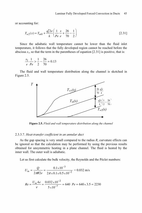
Laminar Fully Developed Forced Convection in Ducts 45
or accounting for:
Tw2(x) Tm0q 12e
k
1
Pe
x
e
26
70
1
2 [2.31]
Since the adiabatic wall temperature cannot be lower than the fluid inlet temperature, it follows that the fully developed region cannot be reached before the abscissa x1, so that the term in the parentheses of equation [2.31] is positive, that is:
x1
e
1
Pe
1
2
26
700.13
The fluid and wall temperature distribution along the channel is sketched in Figure 2.5.
Tw1(x)
Tw2(x)
Tm(x)
T 26
70
q 1e
k
q 1e
k
1
2
26
70
Figure 2.5. Fluid and wall temperature distribution along the channel
2.3.3.7. Heat-transfer coefficient in an annular duct
As the gap spacing is very small compared to the radius R, curvature effects can be ignored so that the calculation may be performed by using the previous results obtained for unsymmetric heating in a plane channel. The fluid is heated by the inner wall. The outer wall is adiabatic.
Let us first calculate the bulk velocity, the Reynolds and the Péclet numbers:
UmQ
2 R2e
0.1x10 3
2 x 0.1x 0.5 x10 2 = 0.032 m/s
ReUm 4e 0.032 x10 2
5 x10 7640 Pe 640 x 3.5 2230
46 Convective Heat Transfer
The heat flux q 1 , supplied by the heating wall, is obtained by dividing the total heat transfer rate by the inner wall surface:
q 1q
2 RL
104
2 x 0.1x115.9 kW/m2 1 2
132.5q e
kC
The following temperatures are deduced from [2.29], [2.30] and [2.31] for the distance x = 1 m:
Tm = 33.7°C, Tw1 = 82.9°C, Tw2
= 16.5°C.
2.4. Flow in a plane channel insulated on one side and heated at uniform temperature on the opposite side
2.4.1. Description of the problem
In an industrial facility, fluid flows through a rectangular channel at the inlet temperature T0 (Figure 2.6). The channel spacing 2e is very small compared to the length Lz in the spanwise direction (e << Lz), so the flow may be considered as two-dimensional. The bulk velocity Um corresponds to the laminar regime. The wall P2 is insulated on its overall length. The wall P1 is insulated up to the section S0 of abscissa x0 and then heated at uniform temperature T1 (T1 > T0 for x x0 ). The section S0 is located far downstream from the channel inlet so that the flow is hydrodynamically fully developed in this region. As a consequence of heating, a thermal boundary layer develops on P1 and reaches the opposite wall P2 at abscissa x1. A thermally fully developed region is observed at some distance downstream from x1. Further downstream, the temperature homogenizes in the channel. The aim of the task is to estimate the distance necessary for the fluid to become nearly isothermal.
u(y)x
y
2e
P2
P1T1
T0Tw(x)
x1x0
Figure 2.6. Flow in a channel insulated on one side and heated at uniform temperature on the opposite side. Notations
Laminar Fully Developed Forced Convection in Ducts 47
Determine the temperature distribution Tw(x) on wall P2 in the thermally fully developed region. Axial conduction effects are assumed to be negligible.
Calculate the distance X x x1 corresponding to the wall temperature difference equal to 1% of its initial value.
The fluid is helium gas of thermal diffusivity 1.6 10-4 m2 s-1; Pr = 0.67. The flow conditions are 2e = 3 mm, Um = 5 m s-1.
2.4.2. Guidelines
Calculate the velocity distribution u(y) in the channel.
Simplify the energy equation when the assumptions indicated previously are taken into account.
Integrate the energy equation over the channel height. It is recommended that dimensionless variables are used.
Propose a dimensionless temperature profile that accounts for the thermal boundary conditions on the two walls (it is suggested a polynomial form is used) and determine the temperature distribution Tw(x) along the channel by using the integral energy equation
2.4.3. Solution
2.4.3.1. Velocity profile
The velocity profile is given by [2.13] in the fully developed laminar regime:
u( )
Um
3
21 2 with
y
e
2.4.3.2. Energy equation
PRELIMINARY NOTE.– The temperature of wall P2 starts to increase for x x1. This situation seems surprising at first view since this wall is insulated and is therefore assumed not to exchange heat with the fluid. However, it must be considered as the limiting case of a very weak heat transfer from the fluid to wall P2 . The steady temperature distribution on P2 corresponds to the thermal equilibrium reached after a very long time. In a practical application, the wall P2 is built of an insulating material so that the heat flux through it is very weak, but not strictly zero. P2 is
48 Convective Heat Transfer
slowly heated up to its equilibrium temperature. The current problem considers the situation of thermal equilibrium where the temperature field is steady.
The energy equation simplifies, as in section 2.3.3.2, as:
u(y)T
x
T
y [2.32]
Normalizing the fluid temperature with that of the wall P1 does not modify this equation, which is integrated from one wall to the other. Since the velocity is independent of x, the integral equation becomes:
d
dxu(y)
e
eT x, y T1 dy
T
ye
e
The temperature gradient T yy e
is zero since the wall P2 is adiabatic. The
bulk temperature [2.8] is introduced into the integral equation as in section 2.3.3.3:
2Umed
dxTm x T1
T
yy e
[2.33]
This equation is then expressed with dimensionless variables. The distance y to P1 was already normalized with the channel half-width as y e . The Péclet number is based on the hydraulic diameter ( Dh 4e ):
PeUm 4e
The abscissa x along the channel is normalized as x x1
4e
1
Pe. The
temperature is normalized by the difference Tw x T1 in a channel cross-section:
,T(x, y) T1
Tw x T1 [2.34]
The dimensionless bulk temperature is calculated by the integral:
m1
2
u
Um11 , d [2.35]
Laminar Fully Developed Forced Convection in Ducts 49
The temperature of wall P2 may also be written in the dimensionless form:
xT1 Tw x
0 with 0 T1 T0 [2.36]
The temperature scale 0 simplifies in the integral equation, which after the transformation of variables becomes:
1
8
d
dm
1
[2.37]
In the fully developed regime, the dimensionless temperature profile is independent of x and the same statement is true for m versus . Finally, the differential equation satisfied by the dimensionless wall temperature yields:
d
d [2.38]
The solution is
exp [2.39]
where the condition 0 0 for x x1 has been accounted for. The Nusselt number is defined by
Nuq 1
kT1 Tm
4e
k T yy e
kT1 Tm
4e
[2.40]
where q 1 is the heat flux at wall P1 . The Nusselt number is constant and, after substituting the dimensionless variables, is given by:
Nu2
4
m 1
[2.41]
2.4.3.3. Approximate solution
An approximate solution is obtained by estimating a temperature profile for calculating the two unknowns m , 1 in equation [2.42] and then obtaining
50 Convective Heat Transfer
the Nusselt number. Some conditions are prescribed to the selected temperature profile in order to obtain a shape close to the physical solution. With definition [2.34], the temperature continuity at the walls implies 1 0 , 1 1.
The adiabaticity condition on wall P2 implies 1 0 .
Among all the possible functions that satisfy these three conditions, it is
convenient to choose a second-degree polynomial 1
42 2 3 .
The bulk temperature is then calculated by using equation [2.35] m = 7/10. Moreover, 1 = 1. Finally, the Nusselt number is obtained by using
equation [2.42], Nu = 40/7 = 5.71.
This approach may be refined by noting that the left-hand side of equation [2.32] is zero on the wall (u = 0) for the exact solution, so that an additional condition may be considered for the approximate temperature profile, 2 2 1 0 . It is possible to account for one or two of these additional conditions by selecting a polynomial of higher degree than the previous approximate solution. The results depend on the degree of the chosen polynomial and are shown in Table 2.2. The third-degree polynomial was determined by taking the condition 2 2 1 0 into account. [SHA 78] indicates Nu = 4.86.
m Nu Deviation relative to [SHA 78]
1 4 2 2 3 0.7 5.71 +17%
1 16 3 3 2 9 11 0.712 4.21 -13%
1 16 4 6 2 8 13 0.743 5.38 +10%
Table 2.2. Flow in a channel insulated on one side and heated at uniform temperature on the opposite side. Nusselt number in fully developed region obtained with the integral method
Figure 2.7 compares the temperature profiles approximated by second- or third- degree polynomials to the exact profile obtained by a series-solution. The second-degree polynomial underestimates the temperature in the half of the channel near the adiabatic wall whereas the third-order polynomial overestimates the temperature in the whole channel.
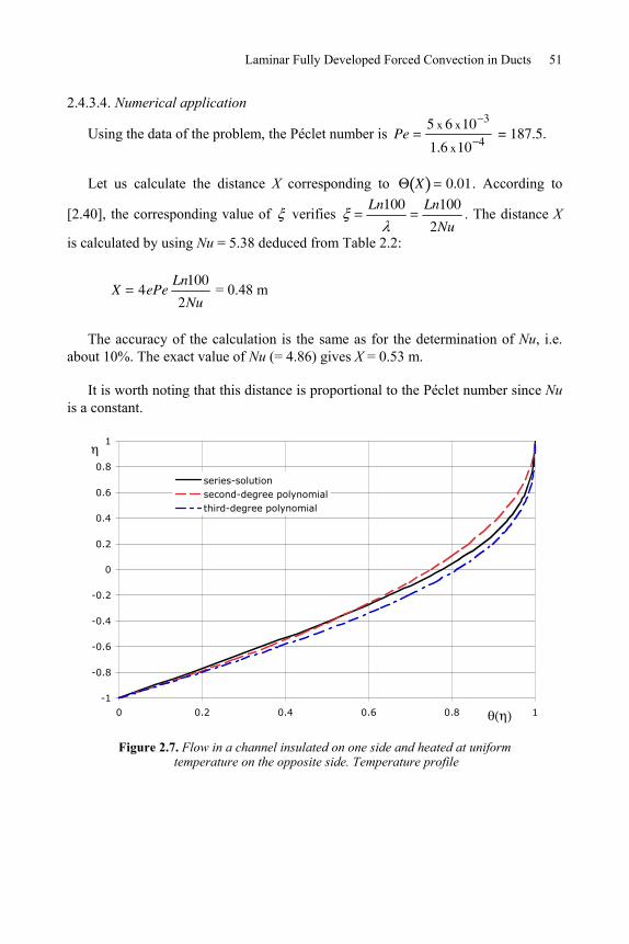
Laminar Fully Developed Forced Convection in Ducts 51
2.4.3.4. Numerical application
Using the data of the problem, the Péclet number is Pe5 x 6 x10 3
1.6 x10 4 = 187.5.
Let us calculate the distance X corresponding to X 0.01. According to
[2.40], the corresponding value of verifies Ln100 Ln100
2Nu. The distance X
is calculated by using Nu = 5.38 deduced from Table 2.2:
X 4ePeLn100
2Nu = 0.48 m
The accuracy of the calculation is the same as for the determination of Nu, i.e. about 10%. The exact value of Nu (= 4.86) gives X = 0.53 m.
It is worth noting that this distance is proportional to the Péclet number since Nu is a constant.
-1
-0.8
-0.6
-0.4
-0.2
0
0.2
0.4
0.6
0.8
1
0 0.2 0.4 0.6 0.8 1
series-solutionsecond-degree polynomialthird-degree polynomial
Figure 2.7. Flow in a channel insulated on one side and heated at uniform temperature on the opposite side. Temperature profile

This page intentionally left blank
Chapter 3
Forced Convection in Boundary Layer Flows
3.1. Hydrodynamics
Flows at a high Reynolds number are generally characterized by large irrotational regions adjacent to thin boundary layers, which develop on walls and concentrate vorticity and viscosity effects. These velocity boundary layers connect the near-wall region, where the velocity tends to zero at the wall due to the no-slip condition, to the free stream characterized by the external velocity u . The velocity u is given by the theory of potential flows and is the slip velocity at the wall in this model.
Boundary layers are very important because they play a major role in heat transfer phenomena, which take place when the walls and the free stream have different temperatures. In fact, the near-wall flow mainly controls the heat exchange at a high Reynolds number. As for velocity, the fluid temperature variations are concentrated in a very thin near-wall region, called the thermal boundary layer. This region constitutes the main contribution to the thermal resistance between the wall and the fluid.
3.1.1. Prandtl equations
The Navier-Stokes equations simplify in boundary layers because the transverse length scale (boundary layer thickness ) is much shorter than the longitudinal length scale (abscissa x or wall length L). For a two-dimensional constant-property
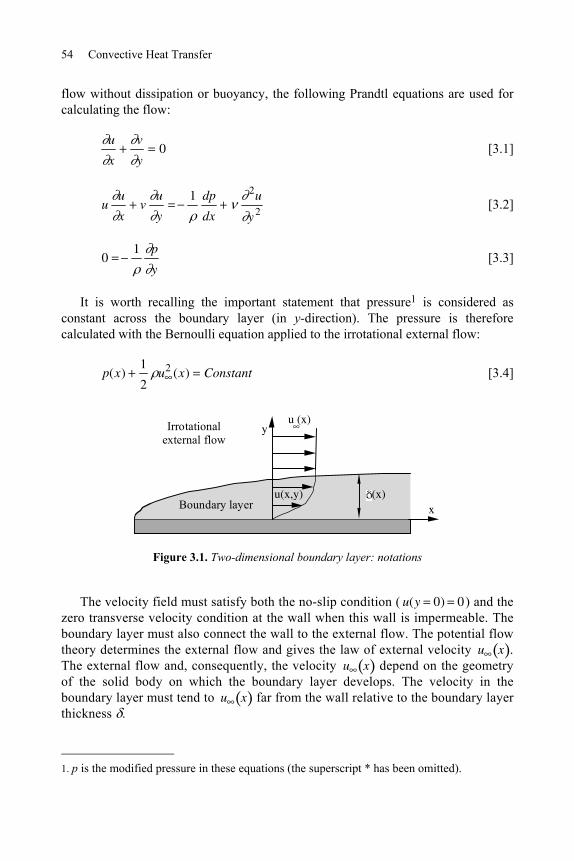
54 Convective Heat Transfer
flow without dissipation or buoyancy, the following Prandtl equations are used for calculating the flow:
u
x
v
y0
[3.1]
uu
xv
u
y
1 dp
dx
2u
y2
[3.2]
01 p
y [3.3]
It is worth recalling the important statement that pressure1 is considered as constant across the boundary layer (in y-direction). The pressure is therefore calculated with the Bernoulli equation applied to the irrotational external flow:
p(x)1
2u2 (x) Constant
[3.4]
y
x(x)u(x,y)
u (x)Irrotational external flow
Boundary layer
Figure 3.1. Two-dimensional boundary layer: notations
The velocity field must satisfy both the no-slip condition ( u(y 0) 0 ) and the zero transverse velocity condition at the wall when this wall is impermeable. The boundary layer must also connect the wall to the external flow. The potential flow theory determines the external flow and gives the law of external velocity u x . The external flow and, consequently, the velocity u x depend on the geometry of the solid body on which the boundary layer develops. The velocity in the boundary layer must tend to u x far from the wall relative to the boundary layer thickness .
1. p is the modified pressure in these equations (the superscript * has been omitted).
Forced Laminar Boundary Layer Flows 55
3.1.2. Classic results
3.1.2.1. Scale analysis
Considering the Prandtl equations, scale analysis shows that the velocity boundary layer thickness verifies the relationship:
(x)
x
1
Re(x) [3.5]
with Re(x)u (x)x
. The symbol means that the two sides of equation [3.5] have
the same order of magnitude (apart from a numerical coefficient of the order of 1).
In the same way, the shear stress exerted by the fluid on the wall is estimated by
0 (x)u(x, y)
y y 0
u (x)
(x)
[3.6]
where (x) is given by [3.5].
3.1.2.2. Blasius boundary layer
The simplest type of boundary layer corresponds to uniform velocity external flow along a plane plate. In these conditions, equation [3.5] shows that the boundary layer thickness grows as a parabolic function against x. The 0.99 thickness is defined as the distance to the wall corresponding to u(x, y) 0.99u . The numerical solution of the Prandtl equations gives:
0.99 x
x
4.92
Rex [3.7]
The skin-friction coefficient is given by:
C f x 0(x)
u 2
0.332
Rex [3.8]
3.1.2.3. Influence of pressure gradient
The spatial development of a boundary layer is controlled by the law of external velocity u (x) or, equivalently, by the longitudinal pressure gradient dp(x) dx . For accelerated external flows (flow in a diverging duct, in the downstream region of an obstacle), the boundary layer has a tendency to thin under the influence of the
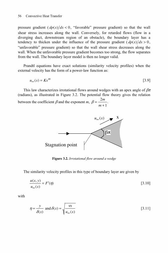
56 Convective Heat Transfer
pressure gradient ( dp(x) dx 0 , “favorable” pressure gradient) so that the wall shear stress increases along the wall. Conversely, for retarded flows (flow in a diverging duct, downstream region of an obstacle), the boundary layer has a tendency to thicken under the influence of the pressure gradient ( dp(x) dx 0 , “unfavorable” pressure gradient) so that the wall shear stress decreases along the wall. When the unfavorable pressure gradient becomes too strong, the flow separates from the wall. The boundary layer model is then no longer valid.
Prandtl equations have exact solutions (similarity velocity profiles) when the external velocity has the form of a power-law function as:
u (x) Kxm [3.9]
This law characterizes irrotational flows around wedges with an apex angle of (radians), as illustrated in Figure 3.2. The potential flow theory gives the relation
between the coefficient and the exponent m, 2m
m 1.
xu (x)
Stagnation point
Figure 3.2. Irrotational flow around a wedge
The similarity velocity profiles in this type of boundary layer are given by
u(x, y)
u (x)F ( )
[3.10]
with
y
(x) and (x)
x
u (x) [3.11]
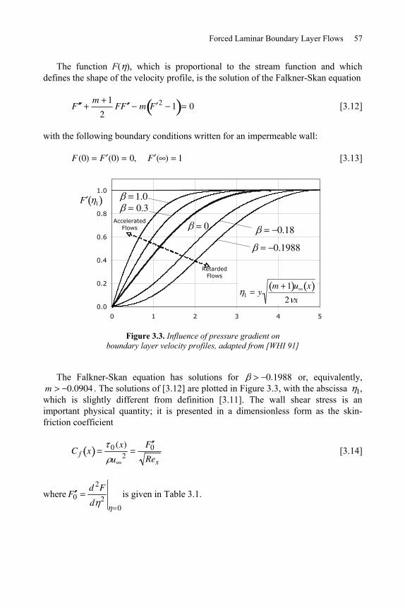
Forced Laminar Boundary Layer Flows 57
The function F( ), which is proportional to the stream function and which defines the shape of the velocity profile, is the solution of the Falkner-Skan equation
F m 1
2FF m F 2 1 0
[3.12]
with the following boundary conditions written for an impermeable wall:
F (0) F (0) 0, F ( ) 1 [3.13]
0.0
0.2
0.4
0.6
0.8
1.0
0 1 2 3 4 5
1.00.3
0 0.18
0.1988
1 ym 1 u x
2 x
Retarded Flows
Accelerated Flows
F 1
Figure 3.3. Influence of pressure gradient on boundary layer velocity profiles, adapted from [WHI 91]
The Falkner-Skan equation has solutions for 0.1988 or, equivalently, m 0.0904 . The solutions of [3.12] are plotted in Figure 3.3, with the abscissa 1, which is slightly different from definition [3.11]. The wall shear stress is an important physical quantity; it is presented in a dimensionless form as the skin-friction coefficient
C f x 0 (x)
u 2
F 0Rex
[3.14]
where F 0d 2F
d 20
is given in Table 3.1.
58 Convective Heat Transfer
-0.1988 -0.18 0 0.3 1
F 0 0 0.087 0.332 0.594 1.232
Table 3.1. Influence of pressure gradient on boundary layer skin-friction (from [WHI 91])
3.2. Heat transfer
3.2.1. Equations of the thermal boundary layer
For very high Péclet numbers ( Pe u L , where L is the longitudinal length scale), heat transfer is concentrated in a thermal boundary layer whose thickness T is much shorter than L. The temperature field verifies the simplified energy equation:
uT
xv
T
y
2T
y2
[3.15]
Boundary conditions depend on the mode of heating. When the wall and external temperatures are prescribed, the boundary conditions are:
T x, y 0 Tw(x) , T x, y T
Equation [3.15] complements the Prandtl equations. The thermal field can be calculated when the velocity field has been determined in a first step.
3.2.2. Scale analysis
The thermal problem is characterized by a typical temperature difference Tw T . The local Nusselt number is defined using the heat flux q 0(x) ,
supplied by the wall to the fluid and by the longitudinal length scale x. The heat-transfer coefficient h (in W m-2 K-1) is related to the heat flux by
q 0(x) h(x) [3.16]
Nuxq 0(x)
k x
h(x)x
k [3.17]
The analysis of equations [3.1], [3.2] and [3.15] gives the order of magnitude of the main variables shown in Table 3.2. It is worth noting that the scale does not play any role in these results, since the thermal problem is linear in temperature.
Forced Laminar Boundary Layer Flows 59
T Nux
Pr << 1 Pr1/2 Rex1/2Pr1/2
Pr > 1 or Pr ~ 1 Pr1/3 Rex1/2Pr1/3
Table 3.2. Results of scale analysis in laminar thermal boundary layers
3.2.3. Similarity temperature profiles
3.2.3.1. Energy equation
For a flow characterized by the external velocity law of the form u (x) Kxm , energy equation [3.15] has similarity solutions if the wall temperature also has the form of a power-law function Tw(x) T Hxn . In this case, the temperature profile is:
T(x, y) T
Tw (x) T( )
[3.18]
The dimensionless distance to the wall is defined by equation [3.11]. The function ( ) , which defines the shape of the temperature profile, satisfies
m 1
2PrF nPrF 0
[3.19]
with the boundary conditions
(0) 1, ( ) 0
The solution of [3.19] depends on m, n and Pr. The wall heat flux is deduced from the temperature field. Setting 0 (0) , it is expressed as
q 0(x) kT
y y 0
k Tw(x) Tu (x)
x0 m, n, Pr
[3.20]
and the Nusselt number is inferred from the above equation using definition [3.17] ( 0 0).
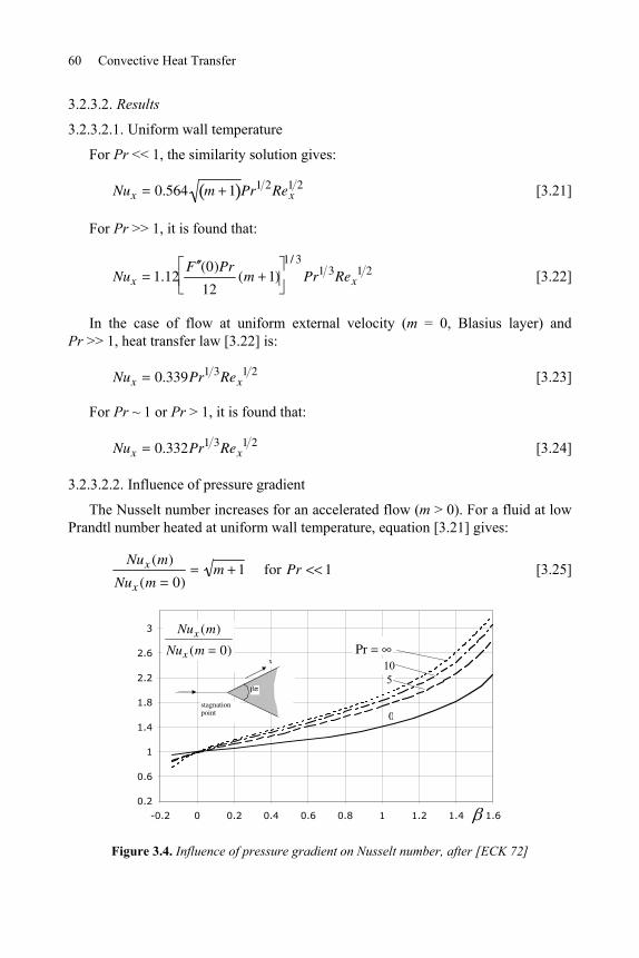
60 Convective Heat Transfer
3.2.3.2. Results
3.2.3.2.1. Uniform wall temperature
For Pr << 1, the similarity solution gives:
Nux 0.564 m 1 Pr1 2Rex1 2
[3.21]
For Pr >> 1, it is found that:
Nux 1.12F (0)Pr
12(m 1)
1/ 3
Pr1 3Rex1 2
[3.22]
In the case of flow at uniform external velocity (m = 0, Blasius layer) and Pr >> 1, heat transfer law [3.22] is:
Nux 0.339Pr1 3Rex1 2
[3.23]
For Pr ~ 1 or Pr > 1, it is found that:
Nux 0.332Pr1 3Rex1 2
[3.24]
3.2.3.2.2. Influence of pressure gradient
The Nusselt number increases for an accelerated flow (m > 0). For a fluid at low Prandtl number heated at uniform wall temperature, equation [3.21] gives:
Nux (m)
Nux (m 0)m 1 for Pr 1
[3.25]
0.2
0.6
1
1.4
1.8
2.2
2.6
3
-0.2 0 0.2 0.4 0.6 0.8 1 1.2 1.4 1.6
Pr105
0
Nux (m)
Nux (m 0)x
stagnation point
Figure 3.4. Influence of pressure gradient on Nusselt number, after [ECK 72]
Forced Laminar Boundary Layer Flows 61
-0.199 -0.18 0 0.3 1
Pr m -0.090 -0.083 0 0.176 1
0.01 0.882 0.915 1 1.108 1.473
0.1 0.787 0.857 1 1.145 1.568
0.72 0.680 0.789 1 1.192 1.696
2 0.625 0.755 1 1.215 1.761
6 0.571 0.724 1 1.235 1.818
10 0.547 0.712 1 1.242 1.839
100 0.451 0.670 1 1.263 1.900
Table 3.3.
Nux (m) Nux (m 0) as a function of Pr and from [WHI 91]
Figure 3.4 shows the Nusselt number for a fixed value of the exponent m, normalized by the result obtained for a plate with zero pressure gradient (m = 0). The velocity of the reference flow is chosen as equal to the local velocity of the actual flow (Kxm). Heating is performed at uniform wall temperature. The ratio Nux (m) Nux (m 0)
is also given by Table 3.3. It is worth noting that the heat-transfer coefficient is significantly increased in the case of a strong favorable pressure gradient. The computation of Nu is no longer possible for 0.1988 (condition for flow separation).
3.2.3.2.3. Influence of heating mode
Equation [3.20] shows that similarity solutions to [3.19] exist for uniform flow (m = 0) when q 0(x) varies as xn 1 2. Hence, heating with uniform wall heat flux ( n 1 2 ) is a particular case of such heating modes. The wall temperature varies as x1 2 in this mode of heating. For a flow with zero pressure gradient (m = 0) and uniform wall flux heating, the increase in Nu is ([ECK 72]):
Nux (n 1 2)
Nux (n 0)1.31
[3.26]
Nux 0.435Pr1 3Rex1 2 for n 1 2 [3.27]
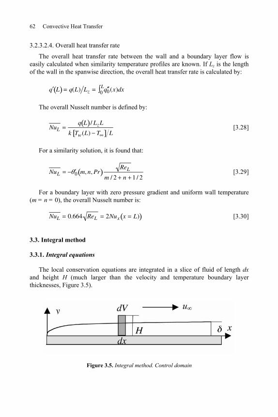
62 Convective Heat Transfer
3.2.3.2.4. Overall heat transfer rate
The overall heat transfer rate between the wall and a boundary layer flow is easily calculated when similarity temperature profiles are known. If Lz is the length of the wall in the spanwise direction, the overall heat transfer rate is calculated by:
q L q(L) Lz q 00L (x)dx
The overall Nusselt number is defined by:
NuLq L / LzL
k Tw(L) T L [3.28]
For a similarity solution, it is found that:
NuL 0 m, n, PrReL
m / 2 n 1 / 2 [3.29]
For a boundary layer with zero pressure gradient and uniform wall temperature (m = n = 0), the overall Nusselt number is:
NuL 0.664 ReL 2Nux x L) [3.30]
3.3. Integral method
3.3.1. Integral equations
The local conservation equations are integrated in a slice of fluid of length dx and height H (much larger than the velocity and temperature boundary layer thicknesses, Figure 3.5).
Figure 3.5. Integral method. Control domain
Forced Laminar Boundary Layer Flows 63
For incompressible flow, the momentum equation yields in the control domain:
tudy0
H
xu u u (x) dy0
H
du (x)
dxu (x) u dy0
H u
y 0
[3.31]
In steady regime ( t 0 ), the Karman equation is obtained
d u (x)
dx
u (x)
u (x)2 u (x) *(x) C f (x)
[3.32]
with the following definitions:
– displacement thickness *(x) 1u(x, y)
u (x)0 dy
– momentum thickness u (x)u(x, y)
u (x)1
u(x, y)
u (x)0 dy
– skin-friction coefficient C f (x) 0 (x)
u (x)2
The integral energy equation reads for the same control domain
t 0H C pTdy
x 0H C pu T T dy q 0 x k
T
y y 0 [3.33]
where q 0 x is the local heat flux. In a steady regime, this equation may be written (Pohlhausen equation)
u (x) d h2
dx2 h
2 du (x)
dx
2
Prh
c [3.34]
with the following definitions:
– convection thickness h (x)T(x, y) T
Tw(x) T
u(x, y)
u (x)0 dy ;
– conduction thickness c (x)
Tw(x) T
T y 0
64 Convective Heat Transfer
3.3.2. Principle of resolution using the integral method
The integral method is an approximate method, which makes it possible to calculate global quantities (skin-friction coefficient, heat-transfer coefficient) with a reasonable accuracy. Concerning hydrodynamics, the problem consists of one equation ([3.32]) in three unknowns: *(x) , u (x) and C f x . An approximate velocity profile is selected to approach at best the shape of the exact one. Some conditions are prescribed for the velocity profile in this purpose. A polynomial function is conveniently selected for the shape of the velocity profile. For example, the following third-degree polynomial is often used in the velocity boundary layer
u(x, y)
u (x)f ( )
3
2
3
2
( ) 1 for 1 [3.35]
with y (x), where (x) is proportional to the velocity boundary layer thickness. The polynomial selected above satisfies the conditions
f (0) f (1) f (0) 0, f (1) 1
which express the no-slip condition for an impermeable wall and matching conditions with the free stream. The condition f (0) 0 is a consequence of the local Prandtl equation in x-direction, written in y = 0, for a flow with zero pressure gradient. The three unknowns *(x) , u (x) and C f x are expressed as functions of (x) by using their definitions. Replacing the result in equation [3.32], an equation in one unknown (x) is obtained. The initial value of the boundary layer thickness is given by (x0) 0. Solving the new equation gives (x) and consequently the quantities to be calculated, *(x) , u (x) and C f x .
The principle of resolution is the same for the thermal problem. In this case, a temperature profile is selected, for example of the polynomial form
T(x, y) T
Tw (x) T( ) 1
3
2
3
2 for 1 [3.36]
( ) 0 for 1
Forced Laminar Boundary Layer Flows 65
with y T (x) , where T (x) is proportional to the thermal boundary layer thickness. The polynomial selected above satisfies the conditions:
(0) 1, (1) (0) (1) 0
The method is then the same as for hydrodynamics. The unknowns h (x) and c (x) are expressed as functions of T (x) and the results are reported in equation
[3.34]. Solving the new equation gives T (x) and, consequently, the quantities to be determined. The heat-transfer coefficient is deduced from the conduction thickness, according to its definition:
h(x)k
c (x) [3.37]
The boundary condition that T (x) must satisfy also concerns the beginning of the thermal boundary layer and is of the form T (x1) 0. The integral method is very convenient for solving the Eckert problem, where the start of heating is shifted downstream relative to the beginning of the velocity boundary layer ( x1 x0).
As an example, the integral method may be checked when applied to the Blasius boundary layer. Using profile [3.35], the skin-friction coefficient is found to be
C f0(x)
u 2
0.323
Rex
which is 3% lower than the exact value [3.8]. For heat transfer, when the velocity and temperature boundary layers develop simultaneously ( x1 x0) and, for Pr > 1, the Nusselt number is found to be
Nux 0.332Pr1 3Rex1 2
in perfect agreement with the exact result [3.24]; this coincidence is, however, accidental.
3.4. Heated jet nozzle
3.4.1. Description of the problem
A facility consists of a large tank with a nozzle attached; the nozzle is composed, first, of a converging duct, followed by a cylindrical tube of length L and diameter D (Figure 3.6). The tank is filled with air at pressure p1 and temperature T1, which
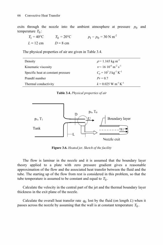
66 Convective Heat Transfer
exits through the nozzle into the ambient atmosphere at pressure p0 and temperature T0 :
T1 = 40°C T0 = 20°C p1 p0 = 30 N m-2
L = 12 cm D = 8 cm
The physical properties of air are given in Table 3.4.
Density = 1.165 kg m-3
Kinematic viscosity = 16 10-6 m-2 s-1
Specific heat at constant pressure Cp = 103 J kg-1 K-1
Prandtl number Pr = 0.7
Thermal conductivity k = 0.025 W m-1 K-1
Table 3.4. Physical properties of air
Figure 3.6. Heated jet. Sketch of the facility
The flow is laminar in the nozzle and it is assumed that the boundary layer theory applied to a plate with zero pressure gradient gives a reasonable approximation of the flow and the associated heat transfer between the fluid and the tube. The starting up of the flow from rest is considered in this problem, so that the tube temperature is assumed to be constant and equal to T0 .
Calculate the velocity in the central part of the jet and the thermal boundary layer thickness in the exit plane of the nozzle.
Calculate the overall heat transfer rate q0 lost by the fluid (on length L) when it passes across the nozzle by assuming that the wall is at constant temperature T0 .
Forced Laminar Boundary Layer Flows 67
3.4.2. Solution
3.4.2.1. Jet exit velocity
A velocity boundary layer develops on the tube wall. As a first approximation, it may be assumed that the boundary layer starts at the tube inlet. A more precise calculation should account for the development of the boundary layer in the converging part of the nozzle. It is also assumed that the boundary layer thickness is much narrower than the tube radius. This issue will be checked at the end of the calculation. These assumptions make it possible to use Bernoulli’s relation between the tank, where the velocities are negligible, and a current point located in the central part of the nozzle exit cross-section, where the velocity is U. It is important to remember that the pressure is constant in a jet cross-section and is therefore equal to the atmospheric pressure p0 at the nozzle exit. The Bernoulli’s relation reads:
p1 p01
2U 2
The exit velocity is deduced from the above equation, U = 7.18 m s-1.
3.4.2.2. Thermal boundary layer thickness
The characteristic Reynolds number is based on the longitudinal length L for a boundary layer flow and not on the tube diameter D, as in the fully developed regime in a duct (Chapter 2).
ReLUL
5.38 x10⁴
The flow is laminar in the tube for this value of the Reynolds number (Chapter 8). Assuming that the results relative to a boundary layer with zero pressure gradient may be applied to the actual flow, the velocity boundary layer thickness is calculated by [3.7]
4.9L
ReL
so that 2.5 mm.
This value is actually much lower that the tube radius (R = 40 mm).
68 Convective Heat Transfer
The thermal boundary layer thickness is obtained by using the order of magnitude given in Table 3.2. For air (Pr = 0.7), the ratio of the velocity and temperature boundary layer thicknesses follows the law
T Pr1 3
so that T 2.9 mm.
3.4.2.3. Overall heat transfer rate lost by the fluid across the tube
The overall Nusselt number is given by equation [3.30]:
NuL 0.664 ReL Pr1 3 136.8
The heat transfer rate lost by the fluid towards the tube wall on length L is calculated by using equation [3.28] with the equivalent transverse length Lz 2 R .
q0 2 Rk T1 T0 NuL = 17.2 W
This heat transfer rate may be compared to the transfer of gas enthalpy q1 by fluid flow to the ambient air:
q1 C pUD2
4T1 T0 = 839 W
We find that q0 represents a loss of 2.1% relative to q1 .
3.5. Asymptotic behavior of thermal boundary layers
3.5.1. Description of the problem
We will consider the behavior of thermal boundary layers for very low or very high Prandtl numbers. The free stream velocity may vary with the longitudinal coordinate x . This external flow is, however, not necessarily of the Falkner-Skan type (section 3.1.2.3). Dissipation is negligible. The fluid is Newtonian and the flow is incompressible. The wall and free stream temperatures are uniform. The two limiting cases are to be considered separately, when Pr 0 and Pr respectively. The main issue is to determine the similarity variable, which results in similarity solutions. Determine the Nusselt number for these two asymptotic limits.
Forced Laminar Boundary Layer Flows 69
3.5.2. Guidelines
The velocity boundary layer thickness is much smaller than the thermal boundary layer thickness when Pr 0 . It is then possible to approximate the actual velocity by u u x in the thermal boundary layer. Write the energy equation by using this approximation. Introduce a function g x and a similarity variable
y g x . Transform the energy equation by using the new variable . Deduce a differential equation for g x , so that the problem has similarity solutions.
For Pr , on the other hand, the situation is inverted and the thermal boundary layer thickness is much smaller than . It is then possible to consider that the velocity varies approximately linearly in the thermal boundary layer. Repeat the same procedure as for Pr 0 .
3.5.3. Solution
3.5.3.1. Very small Prandtl numbers
For Pr 0 , the velocity boundary layer thickness is much smaller than the thermal boundary layer thickness. It is then possible to approximate the actual velocity by u u x in the thermal boundary layer (Figure 3.7). The distribution of the velocity component normal to the wall is deduced from the continuity equation
u
x
v
y
du
x
v
y0
so that
vdu
xy
[3.38]
The energy equation becomes:
uT
xv
T
yu x
T
x
du
xy
T
y
2T
y2
[3.39]
The dimensionless temperature is T T
Tw T.
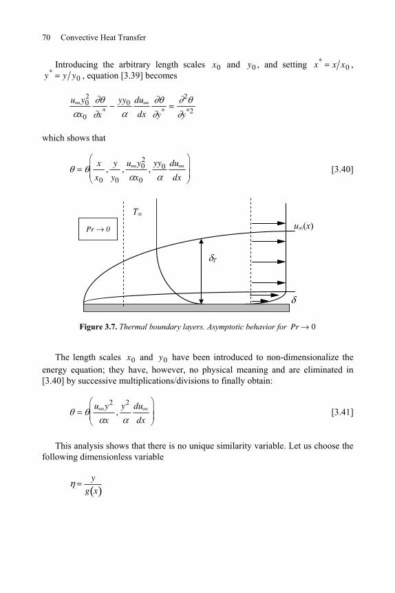
70 Convective Heat Transfer
Introducing the arbitrary length scales x0 and y0 , and setting x* x x0 , y* y y0 , equation [3.39] becomes
u y02
x0 x*
yy0 du
dx y*
2
y*2
which shows that
x
x0
,y
y0
,u y0
2
x0
,yy0 du
dx [3.40]
T
u (x) Pr 0
T
Figure 3.7. Thermal boundary layers. Asymptotic behavior for Pr 0
The length scales x0 and y0 have been introduced to non-dimensionalize the energy equation; they have, however, no physical meaning and are eliminated in [3.40] by successive multiplications/divisions to finally obtain:
u y2
x,
y2 du
dx [3.41]
This analysis shows that there is no unique similarity variable. Let us choose the following dimensionless variable
y
g x
Forced Laminar Boundary Layer Flows 71
and assume that f . The transformation of variables gives
xf
xf yg 2 dg
dx
yf
yf g 1
2
y2f g 2
Substituting these expressions in the energy equation, we find:
1u
dg2
dx2g2 du
dx 2f f 0
[3.42]
Similarity solutions are clearly possible if:
udg2
dx2g2 du
dxConstant
The constant is arbitrary; the resolution of the problem is, however, made easier if the constant is chosen as equal to the fluid thermal diffusivity:
udg2
dx2g2 du
dx [3.43]
With this choice, the dimensionless temperature is the solution to the differential equation:
2f f 0
[3.44]
Multiplying the two sides of equation [3.43] by u , and integrating the resulting equation, the function g(x) is determined by
g(x)1
u xu x1 dx
0
x 1/ 2
[3.45]
72 Convective Heat Transfer
which guarantees the existence of a similarity solution. Integration of [3.44] gives the temperature field:
11
expz2
40dz
[3.46]
The similarity variable is:
yu x u x1 dx0
x 1/ 2
The Nusselt number is easily calculated by
Nuhx
k
d
d 0 yx
and may be presented in the form
Nu11/ 2
u x u x1 dx0
x 1/ 2
x
[3.47]
The Nusselt number on a flat plate in the limit Pr 0 is deduced from the above equation ( u constant )
NuPr Rex
1/ 2
where Rex U x . This approach is a good approximation of heat transfer in liquid metal boundary layers, with or without pressure gradient.
3.5.3.2. Very high Prandtl numbers
Let us now consider the case Pr . For this condition, the following inequality is verified: T , as illustrated by Figure 3.8. The velocity may then be expressed in the thermal boundary layer, by a linear law, as
uu
y 0
y w xy
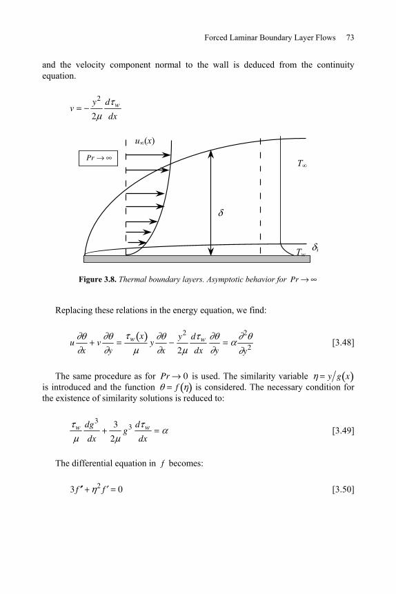
Forced Laminar Boundary Layer Flows 73
and the velocity component normal to the wall is deduced from the continuity equation.
vy2
2
d w
dx
T
u (x)
Pr
TTw
Figure 3.8. Thermal boundary layers. Asymptotic behavior for Pr
Replacing these relations in the energy equation, we find:
ux
vy
w xy
x
y2
2
d w
dx y
2
y2
[3.48]
The same procedure as for Pr 0 is used. The similarity variable y g x is introduced and the function f is considered. The necessary condition for the existence of similarity solutions is reduced to:
w dg3
dx
3
2g3 d w
dx [3.49]
The differential equation in f becomes:
3 f 2 f 0 [3.50]
74 Convective Heat Transfer
The solution of [3.50] is
1 0.5384 expz3
90dz
[3.51]
where y w1/ 2
w1/ 2dx
0
x 1/ 3
.
Consequently, the Nusselt number for Pr is:
Nu 0.5384 w1/ 2
w1/ 2dx
0
x 1/ 3
x
[3.52]
According to Blasius solution
w
u20.332 Rex
1/ 2
on a flat plate. Replacing this expression in [3.52], we find:
Nu 0.3387Pr1/ 3Rex1/2
[3.53]
This relation is valid for a flat plate in the limit Pr .
3.6. Protection of a wall by a film of insulating material
3.6.1. Description of the problem
A flat plate is surrounded by a flow of hot gas parallel to the wall. This arrangement simulates the problem of turbine blades, which must be maintained at a sufficiently low temperature to avoid the destructive effects of very hot fluid in gas turbines. In order to maintain the plate at an acceptable temperature, several channels have been machined in the solid wall. Water passes through these channels to evacuate the heat released by the hot gas to the plate (Figure 3.9).
It is proposed that we calculate the total heat transfer rate between the wall and the external gas in the two following situations:
– when the wall is in direct contact with gas; – when a film of insulating material is placed on the wall surface.
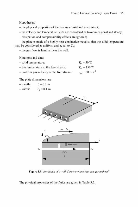
Forced Laminar Boundary Layer Flows 75
Hypotheses: – the physical properties of the gas are considered as constant; – the velocity and temperature fields are considered as two-dimensional and steady; – dissipation and compressibility effects are ignored; – the plate is made of a highly heat-conductive metal so that the solid temperature
may be considered as uniform and equal to T0 ; – the gas flow is laminar near the wall.
Notations and data: – solid temperature: T0 = 50°C – gas temperature in the free stream: T = 150°C – uniform gas velocity of the free stream: u = 30 m s-1
The plate dimensions are: – length: L = 0.1 m – width: Lz = 0.1 m
Figure 3.9. Insulation of a wall. Direct contact between gas and wall
The physical properties of the fluids are given in Table 3.5.
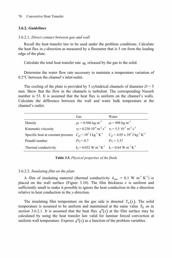
76 Convective Heat Transfer
3.6.2. Guidelines
3.6.2.1. Direct contact between gas and wall
Recall the heat transfer law to be used under the problem conditions. Calculate the heat flux in y-direction as measured by a fluxmeter that is 5 cm from the leading edge of the plate.
Calculate the total heat transfer rate q0 released by the gas to the solid.
Determine the water flow rate necessary to maintain a temperature variation of 0.2°C between the channel’s inlet/outlet.
The cooling of the plate is provided by 5 cylindrical channels of diameter D = 5 mm. Show that the flow in the channels is turbulent. The corresponding Nusselt number is 53. It is assumed that the heat flux is uniform on the channel’s walls. Calculate the difference between the wall and water bulk temperature at the channel’s outlet.
Gas Water
Density f = 0.946 kg m-3 l = 988 kg m-3
Kinematic viscosity f = 0.230 10-4 m-2 s-1l = 5.5 10-7 m-2 s-1
Specific heat at constant pressure Cpf = 103 J kg-1 K-1 Cpl = 4.05 x 10³ J kg-1 K-1
Prandtl number Prf = 0.7 Prl = 3.57
Thermal conductivity kf = 0.032 W m-1 K-1 kl = 0.64 W m-1 K-1
Table 3.5. Physical properties of the fluids
3.6.2.2. Insulating film on the plate
A film of insulating material (thermal conductivity kins = 0.1 W m-1 K-1) is placed on the wall surface (Figure 3.10). The film thickness e is uniform and sufficiently small to make it possible to ignore the heat conduction in the x-direction relative to heat conduction in the y-direction.
The insulating film temperature on the gas side is denoted Tw x . The solid temperature is assumed to be uniform and maintained at the same value T0 as in section 3.6.2.1. It is assumed that the heat flux q x at the film surface may be calculated by using the heat transfer law valid for laminar forced convection at uniform wall temperature. Express q x as a function of the problem variables.
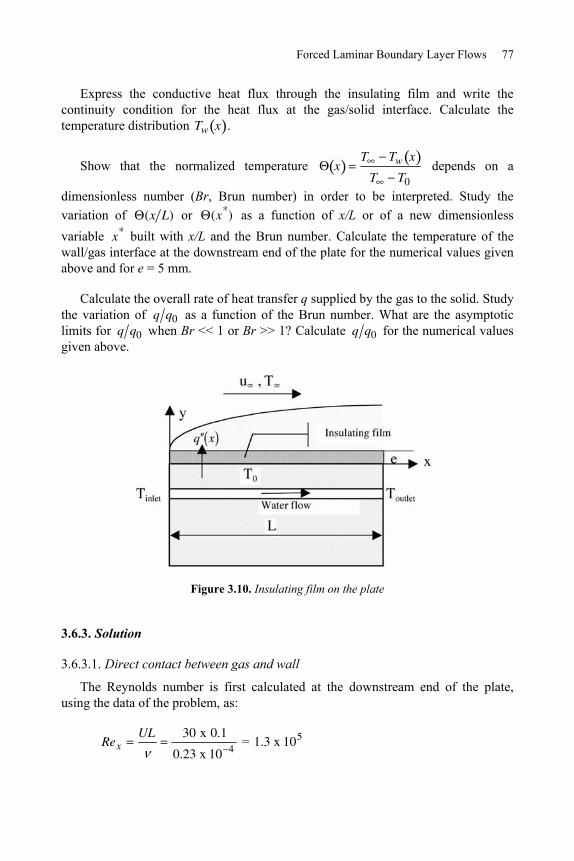
Forced Laminar Boundary Layer Flows 77
Express the conductive heat flux through the insulating film and write the continuity condition for the heat flux at the gas/solid interface. Calculate the temperature distribution Tw x .
Show that the normalized temperature xT Tw x
T T0
depends on a
dimensionless number (Br, Brun number) in order to be interpreted. Study the variation of (x L) or (x*) as a function of x/L or of a new dimensionless variable x*
built with x/L and the Brun number. Calculate the temperature of the wall/gas interface at the downstream end of the plate for the numerical values given above and for e = 5 mm.
Calculate the overall rate of heat transfer q supplied by the gas to the solid. Study the variation of q q0 as a function of the Brun number. What are the asymptotic limits for q q0 when Br << 1 or Br >> 1? Calculate q q0 for the numerical values given above.
Figure 3.10. Insulating film on the plate
3.6.3. Solution
3.6.3.1. Direct contact between gas and wall
The Reynolds number is first calculated at the downstream end of the plate, using the data of the problem, as:
RexUL 30 x 0.1
0.23 x 10 4 = 1.3 x 10⁵
78 Convective Heat Transfer
The laminar-turbulent transition is taking place for Rex ~ 3 x 10⁵ in a boundary layer with zero pressure gradient; the gas flow is laminar along the plate.
3.6.3.1.1. Heat flux
Heat transfer between the wall and the gas flow is governed by the law relative to laminar boundary layers with zero pressure gradient at uniform wall temperature [3.24]:
Nux 0.332Prf1 3Rex
1 2 [3.54]
In the section of the fluxmeter (x = 0.05 m), we find
Rexu x
f
30 x 0.05
0.23 x 10 4 = 6.52 x 10⁴
so that Nux = 75.3.
The local heat-transfer coefficient is deduced from [3.17]
h Nuxk f
x = 75.3 x
0.032
0.05 = 48.2 W m-2 K-1.
and, according to [3.16], q x 0.05m = 48.2 x (150-50) = 4818 W m-2
3.6.3.1.2. Total heat transfer rate on the plate
The total heat transfer rate q0 received by the plate is obtained from equations [3.28] and [3.30] as:
NuL 0.664 ReL = 0.664 1.3 x 105 = 213
The average heat-transfer coefficient is calculated by:
h Nuk f
L = 213 x
0.032
0.1 = 68.1 W m-2 K-1
q0 hLLz T T0 = 68.1 x 0.1 x 0.1 x (150-50) = 68.1 W
Forced Laminar Boundary Layer Flows 79
3.6.3.1.3. Increase in the cooling water temperature
The heat budget is written between the channel’s inlet/outlet. We assume that the total heat transfer rate received by the plate surface is evacuated by the cooling water (there are no heat losses)
q0 lC plQ Toutlet Tinlet [3.55]
where Q, Tinlet and Toutlet denote the water flow rate and the temperature at the channel’s inlet/outlet respectively.
The water flow rate necessary to maintain a temperature variation of 0.2°C between the channel’s inlet/outlet is deduced from the above equation as:
Qq0
lC pl Toutlet Tinlet
= 68,1
988 x 4.05 x 103 x 0.2 = 8.5 x 10⁻⁵ m-3 s-1
where Q = 5.1 l min-1.
3.6.3.1.4. Temperature variations in a cross-section of the cooling channels
The flow rate in a cooling channel is Q 5 = 1.7 x 10⁻⁵ m-3 s-1 and the bulk
velocity is UmQ 5
D2 4 = 0.86 m s-1. The Reynolds number characteristic of the
flow in a channel is:
ReUm D
l
= 0.86 x 0.005
5.5 x 10 7 = 7820.
The flow is therefore turbulent in the channels (Chapter 7). With Nuchannels = 53,
the heat-transfer coefficient is h Nuchannelskl
D = 53 x
0.64
0.005 = 6784 Wm-2 K-1.
Assuming that the heat flux is uniform on the channels surface, it is given by:
q channelsq0
5 DL = 8658 W m-2
80 Convective Heat Transfer
At the outlet, where the thermal regime is supposed to be fully developed ( Nuchannels= 53), the difference between the wall and water bulk temperatures is given by:
Tw Tmq channels
h =
8658
6784 = 1.28°C
Since this temperature difference is weak, it is justifiable to ignore the coupling phenomenon between convection in the channels and conduction in the solid plate.
3.6.3.2. Film of insulating material on the wall surface
3.6.3.2.1. Temperature of the wall/fluid interface
An approximate solution consists of assuming that the convective heat transfer on the wall surface is governed by the law relative to a laminar boundary layer on a plate heated at uniform temperature. The convective heat flux is then deduced from [3.24] as:
q conv (x) 0.332Prf1 3Rex
1 2 k f
xT Tw(x)
[3.56]
It is convenient to introduce the reference heat flux
q L 0.332Prf1 3ReL
1 2 k f
LT T0 hL T T0
where hL is the heat-transfer coefficient for x = L ( hL h 2 , for an isothermal wall,
according to [3.30]). Introducing the dimensionless temperature xT Tw x
T T0
,
equation [3.56] becomes
q conv (x)q Lx L
(x) h(x) (x) T T0
[3.57]
where h(x) is the heat-transfer coefficient at abscissa x.
The conductive heat flux across the insulating film is calculated with the Fourier law. Assuming that the heat flux is mainly in the perpendicular direction to the film, it may simply be written as
q cond (x) kinsTw(x) T0
e [3.58]
Forced Laminar Boundary Layer Flows 81
or, denoting q ins kinsT T0
e,
q cond (x) q ins 1 (x) [3.59]
The heat flux must be continuous at the gas/wall interface:
q conv (x) q cond (x) q (x)
Using equations [3.57] and [3.59], the interface temperature distribution is obtained as
(x)1
1 Br(x) [3.60]
where the dimensionless Brun2 number has been introduced
Br(x)q L
q ins x L [3.61]
When the Brun number Br(x) is written in the form
Br(x)0.332Pr1 3ReL
1 2 k f L x L 1 2
kins e
h(x)
kins e
it is clearly seen that it represents the ratio of the convective to the conductive thermal resistance for heat transfer between the fluid and the solid.
The wall temperature variations are obtained as a function of x, or in a condensed
form, by denoting BrLq Lq ins
hL
kins e
and x* x L
BrL2
.
(x*)x*
1 x*
[3.62]
The above calculation is, however, a rather crude approximation since it uses the heat transfer law valid for uniform wall temperature whereas the resulting wall temperature is a function of x. [LUI 74] and [LIM 92] have performed more accurate
2. This is also a Biot number.
82 Convective Heat Transfer
computations by taking the coupling between convection and conduction into account. Lim and co-authors [LIM 92] have investigated the problem of optimizing insulation with a film of variable thickness along the plate.
Equation [3.62] shows that the gas/wall interface temperature Tw is equal to T ( 0) for x = 0. In this initial region, the convective thermal resistance is negligible relative to the conductive thermal resistance of the insulating film. The solid is only protected by the film, which prevents excessive heat flux. While the boundary layer develops along the plate, the corresponding thermal resistance increases and the surface temperature Tw decreases. If the value reached by x* at the end of the plate is sufficiently high, the surface temperature becomes close to T0 . This means that the heat flux between the gas and the plate becomes very weak and that the temperature drop is concentrated in the boundary layer whose thermal resistance is predominant.
With the data of the problem, BrLhLe
kins
34 x 5 x 10 3
0.1 = 1.7. At the
downstream end of the plate, x* 1 BrL2 1 1.72 = 0.346. According to [3.62],
(x L) = 0.37. The surface temperature is 113 °C.
3.6.3.2.2. Total heat transfer rate
The total heat transfer rate q released by the gas to the solid is obtained by integrating one of the two equations [3.57] or [3.59].
For example, [3.57] and [3.62 give the following law for the heat flux
q (x)q LBrL
1
1 x*
[3.63]
and, after transformation of variables, the total rate of heat transfer is calculated by
q q LLzLBrL1
1 x*01 BrL
2
dx*
[3.64]
It is easily shown that: 1
1 x*dx* 2 x* Ln 1 x*
Forced Laminar Boundary Layer Flows 83
The total rate of heat transfer is:
q 2q LLzL 1 BrLLn 11
BrL [3.65]
The heat transfer rate exchanged in the case of direct contact is obtained for e = 0, namely for BrL 0 , q0 2q LLzL .
Finally, the total heat transfer rate may be written in the form:
q
q0
1 BrLLn 11
BrL [3.66]
This model provides the asymptotic trends:
BrL 1q
q0
1 BrLLn BrL
[3.67]
BrL 1q
q0
1
2BrL [3.68]
with BrL = 1.7, q q0 = 0.21.
The total heat transfer rate received by the plate is reduced by about 80% due to the insulating film.
3.7. Cooling of a moving sheet
3.7.1. Description of the problem
The problem of cooling a solid strip of metal moving in surrounding fluid is present in several industrial processes. We assume that the fluid is at rest far from the moving strip, so that cooling is due to convective heat transfer in the boundary layer generated on the strip surface. Some other cooling processes are clearly more efficient (impacting jets, for example), but are not investigated in this problem.
In order to determine the heat-transfer coefficient for the fluid/solid strip exchange, let us consider the two-dimensional problem of a strip (Figure 3.11) at uniform temperature Tw , moving at constant velocity U in a constant-property fluid (kinematic viscosity , density , thermal conductivity k). Buoyancy and dissipation
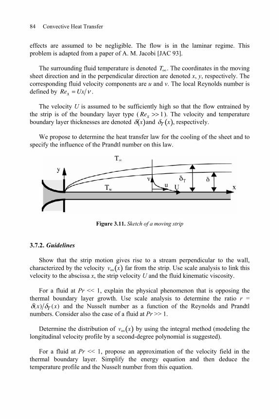
84 Convective Heat Transfer
effects are assumed to be negligible. The flow is in the laminar regime. This problem is adapted from a paper of A. M. Jacobi JAC 93 .
The surrounding fluid temperature is denoted T . The coordinates in the moving sheet direction and in the perpendicular direction are denoted x, y, respectively. The corresponding fluid velocity components are u and v. The local Reynolds number is defined by Rex Ux .
The velocity U is assumed to be sufficiently high so that the flow entrained by the strip is of the boundary layer type ( Rex 1). The velocity and temperature boundary layer thicknesses are denoted x and T x , respectively.
We propose to determine the heat transfer law for the cooling of the sheet and to specify the influence of the Prandtl number on this law.
Figure 3.11. Sketch of a moving strip
3.7.2. Guidelines
Show that the strip motion gives rise to a stream perpendicular to the wall, characterized by the velocity v x far from the strip. Use scale analysis to link this velocity to the abscissa x, the strip velocity U and the fluid kinematic viscosity.
For a fluid at Pr << 1, explain the physical phenomenon that is opposing the thermal boundary layer growth. Use scale analysis to determine the ratio r =
(x) T (x) and the Nusselt number as a function of the Reynolds and Prandtl numbers. Consider also the case of a fluid at Pr >> 1.
Determine the distribution of v x by using the integral method (modeling the longitudinal velocity profile by a second-degree polynomial is suggested).
For a fluid at Pr << 1, propose an approximation of the velocity field in the thermal boundary layer. Simplify the energy equation and then deduce the temperature profile and the Nusselt number from this equation.
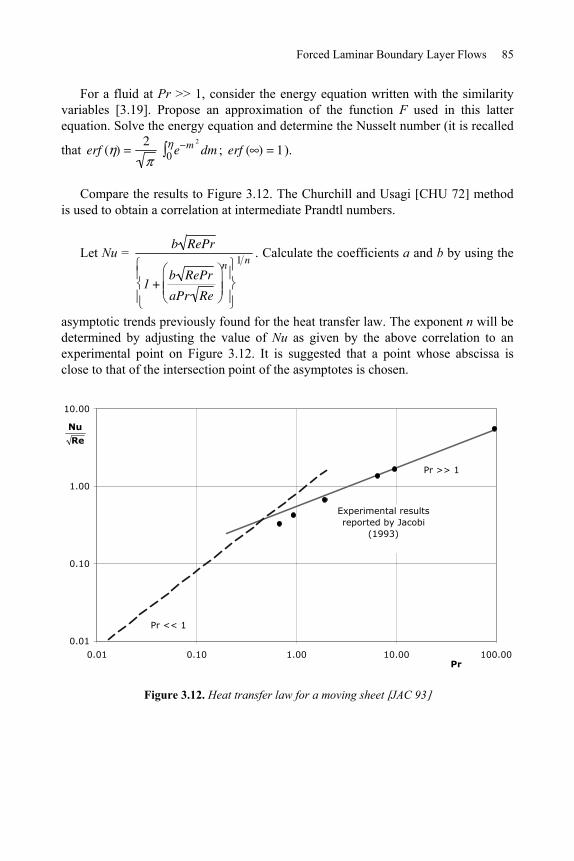
Forced Laminar Boundary Layer Flows 85
For a fluid at Pr >> 1, consider the energy equation written with the similarity variables [3.19]. Propose an approximation of the function F used in this latter equation. Solve the energy equation and determine the Nusselt number (it is recalled
that erf ( )2
e m 2
0 dm ; erf ( ) 1).
Compare the results to Figure 3.12. The Churchill and Usagi CHU 72 method is used to obtain a correlation at intermediate Prandtl numbers.
Let Nu = b RePr
1 +b RePr
aPr Re
n 1 n. Calculate the coefficients a and b by using the
asymptotic trends previously found for the heat transfer law. The exponent n will be determined by adjusting the value of Nu as given by the above correlation to an experimental point on Figure 3.12. It is suggested that a point whose abscissa is close to that of the intersection point of the asymptotes is chosen.
0.01
0.10
1.00
10.00
0.01 0.10 1.00 10.00 100.00Pr
Nu
Re
Pr >> 1
Pr << 1
Experimental results reported by Jacobi
(1993)
Figure 3.12. Heat transfer law for a moving sheet JAC 93
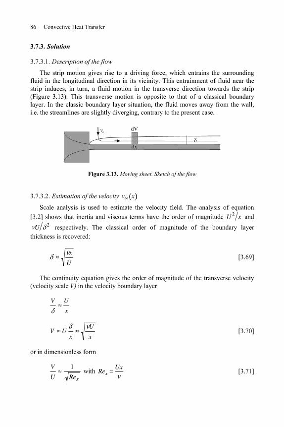
86 Convective Heat Transfer
3.7.3. Solution
3.7.3.1. Description of the flow
The strip motion gives rise to a driving force, which entrains the surrounding fluid in the longitudinal direction in its vicinity. This entrainment of fluid near the strip induces, in turn, a fluid motion in the transverse direction towards the strip (Figure 3.13). This transverse motion is opposite to that of a classical boundary layer. In the classic boundary layer situation, the fluid moves away from the wall, i.e. the streamlines are slightly diverging, contrary to the present case.
Figure 3.13. Moving sheet. Sketch of the flow
3.7.3.2. Estimation of the velocity v x
Scale analysis is used to estimate the velocity field. The analysis of equation [3.2] shows that inertia and viscous terms have the order of magnitude U 2 x and
U 2 respectively. The classical order of magnitude of the boundary layer thickness is recovered:
x
U [3.69]
The continuity equation gives the order of magnitude of the transverse velocity (velocity scale V) in the velocity boundary layer
V U
x
V Ux
U
x [3.70]
or in dimensionless form
V
U
1
Rex
with RexUx
[3.71]
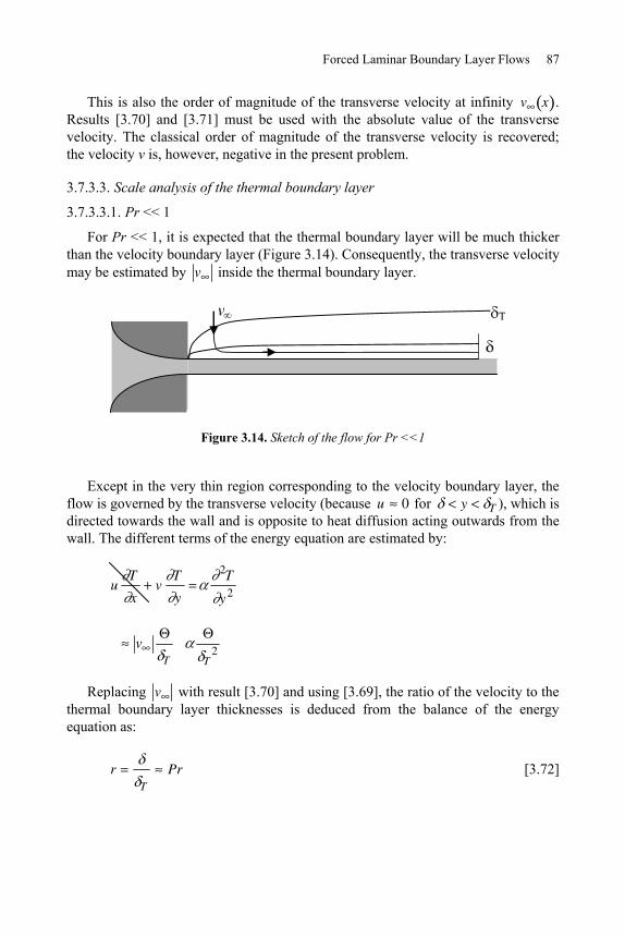
Forced Laminar Boundary Layer Flows 87
This is also the order of magnitude of the transverse velocity at infinity v x . Results [3.70] and [3.71] must be used with the absolute value of the transverse velocity. The classical order of magnitude of the transverse velocity is recovered; the velocity v is, however, negative in the present problem.
3.7.3.3. Scale analysis of the thermal boundary layer
3.7.3.3.1. Pr << 1
For Pr << 1, it is expected that the thermal boundary layer will be much thicker than the velocity boundary layer (Figure 3.14). Consequently, the transverse velocity may be estimated by v inside the thermal boundary layer.
Figure 3.14. Sketch of the flow for Pr <<1
Except in the very thin region corresponding to the velocity boundary layer, the flow is governed by the transverse velocity (because u 0 for y T ), which is directed towards the wall and is opposite to heat diffusion acting outwards from the wall. The different terms of the energy equation are estimated by:
uT
xv
T
y
2T
y2
vT
T
2
Replacing v with result [3.70] and using [3.69], the ratio of the velocity to the thermal boundary layer thicknesses is deduced from the balance of the energy equation as:
rT
Pr
[3.72]
88 Convective Heat Transfer
The Nusselt number is estimated by:
Nuq
k x
k T
k x
x
T
Accounting for [3.75], scale analysis finally gives:
Nu Re1 2Pr [3.73]
3.7.3.3.2. Pr >> 1
For Pr >> 1, conversely to the previous case, it is expected that the velocity boundary layer is much thicker than the thermal boundary layer and, consequently, that velocities are much smaller than v in the present case. In fact, the continuity equation reads:
u
x
v
y0
The longitudinal velocity is constant on the strip wall so that u xy 0 0 and,
therefore, v yy 0 0
A development in series of the velocity v near the wall gives:
v y v 0v
y 0
y2v
y20
y2
2.....
The first two terms are zero; 2v
y20
is estimated by v
2. The transverse velocity
is therefore estimated in the thermal boundary layer by:3
v TU
xT
2
2 [3.74]
Let V1 v T .
Equation [3.74] shows that the order of magnitude of the transverse velocity V1 is much smaller than v ([3.70]) when T , as expected for Pr >> 1. 3. For sake of consistency, this estimation is written without numerical coefficients.
Forced Laminar Boundary Layer Flows 89
Taking this result into account, the different terms of the energy equation are estimated by:
uT
xv
T
y
2T
y2
U
x
U
xT
T2
The dominant term of the left-hand side is the first one, which represents advection in the longitudinal direction. The thermal boundary layer thickness is given by
T2 x
U [3.75]
and the ratio of the boundary layer thicknesses is
rT
Pr1 2
[3.76]
The Nusselt number is estimated as in the previous case and is found as:
Nu Re1 2Pr1 2 [3.77]
3.7.3.4. Calculation of the transverse velocity at infinity with the integral method
The conservation of flow rate is written for a slice dV of length dx, height H and unit depth in the spanwise direction (Figure 3.13)
d u(x, y)dy0H v (x)dx 0
from which, we infer the transverse velocity at infinity
v (x)d
dxu(x,y)dy
H
[3.78]
The velocity profile is modeled by using a second-degree polynomial,
u(x, y)
Uf ( ) a2
2 a1 a0 with y
(x)
90 Convective Heat Transfer
The coefficients of this polynomial are determined with the following conditions:
f (0) 1, f (1) f (1) 0
The result f ( ) 1 2 is reported in equation [3.78], which gives the transverse velocity at infinity:
v (x)1
3U
d (x)
dx [3.79]
The integral method is also used to calculate (x) . The budget of momentum is written for the control volume dV. In this flow with zero pressure gradient, it reduces to:
d u2 (x, y)dy0H u
y 0
dx
This budget results from the variation of momentum between the cross-sections of abscissas x and x + dx and from the shear stress exerted by the wall on the flow.
Introducing the dimensionless velocity profile and simplifying by , the momentum equation becomes
U 2 d
dx(x) f ( )2 d0
1 U
(x)f (0)
since the velocity U is independent of x. Replacing f by its expression and integrating in x, we find that:
(x)
x
20
Rex
Reporting in [3.79], the transverse velocity at infinity is finally obtained as:
v (x)
U
5
3
1
Rex
0.745
Rex [3.80]
The result of scale analysis ([3.71]) is recovered, as expected; in addition, the integral method has given the numerical coefficient in the relation between v (x) and 1 Rex .
Forced Laminar Boundary Layer Flows 91
3.7.3.5. Determination of the heat transfer law for a fluid at Pr << 1
Taking into account the relative thicknesses of the velocity and thermal boundary layers ([3.72]), the approximation u 0, v v may be made in the energy equation. The resulting equation
vT
y
2T
y2
may be integrated over y and the temperature profile is found as
T(x, y) T
Tw Texp
v (x)y
when the boundary conditions (T(x, y 0) Tw , T(x, y ) T ) are taken into account. Replacing v (x) by the result [3.80], the temperature profile is:
T(x, y) T
Tw Texp 0.745
Uy 1
Rex [3.81]
The Nusselt number is defined by Nuxq (y 0)
k Tw T x and is calculated by
Nux
k T y y 0
k Tw T x. The following heat transfer law is obtained:
Nux 0.745Rex1 2Pr [3.82]
As in the transverse velocity, the result of scale analysis is recovered [3.73] and the numerical coefficient of the heat transfer law is now calculated.
3.7.3.6. Determination of the heat transfer law by using a similarity solution for fluids at Pr >> 1
Considering the hydraulic and thermal conditions of the problem, it is possible to find a similarity solution of form [3.18] to energy equation [3.19], written with m = n = 0:
1
2PrF 0
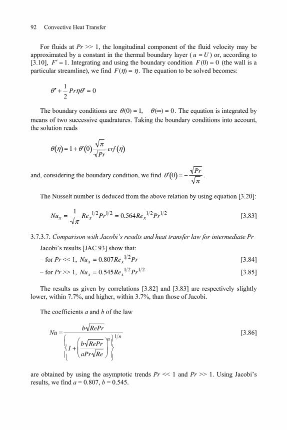
92 Convective Heat Transfer
For fluids at Pr >> 1, the longitudinal component of the fluid velocity may be approximated by a constant in the thermal boundary layer ( u U ) or, according to [3.10], F 1. Integrating and using the boundary condition F (0) 0 (the wall is a particular streamline), we find F ( ) . The equation to be solved becomes:
1
2Pr 0
The boundary conditions are (0) 1, ( ) 0 . The equation is integrated by means of two successive quadratures. Taking the boundary conditions into account, the solution reads
1 0Pr
erf
and, considering the boundary condition, we find 0Pr
.
The Nusselt number is deduced from the above relation by using equation [3.20]:
Nux1
Rex1 2Pr1 2 0.564Rex
1 2Pr1 2
[3.83]
3.7.3.7. Comparison with Jacobi’s results and heat transfer law for intermediate Pr
Jacobi’s results [JAC 93] show that:
– for Pr << 1, Nux 0.807Rex1 2Pr [3.84]
– for Pr >> 1, Nux 0.545Rex1 2Pr1 2
[3.85]
The results as given by correlations [3.82] and [3.83] are respectively slightly lower, within 7.7%, and higher, within 3.7%, than those of Jacobi.
The coefficients a and b of the law
Nu =b RePr
1 +b RePr
aPr Re
n 1 n
[3.86]
are obtained by using the asymptotic trends Pr << 1 and Pr >> 1. Using Jacobi’s results, we find a = 0.807, b = 0.545.
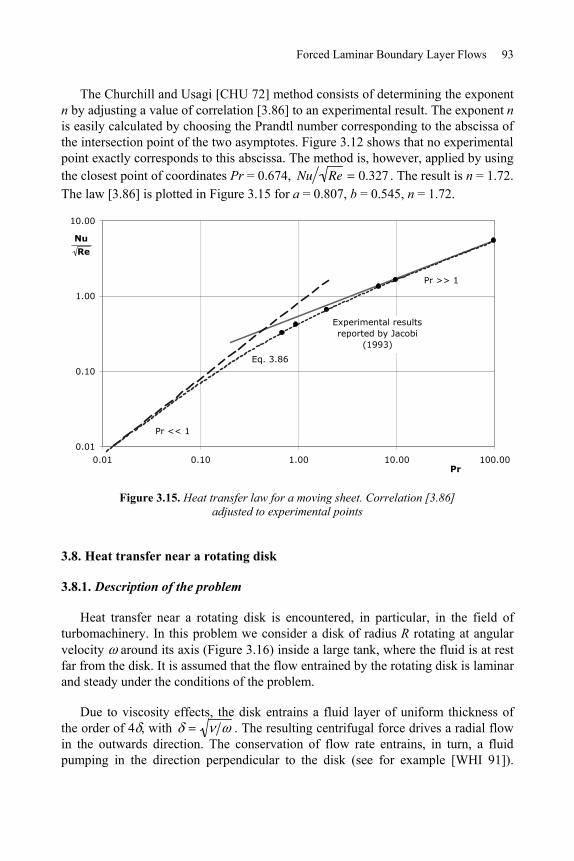
Forced Laminar Boundary Layer Flows 93
The Churchill and Usagi CHU 72 method consists of determining the exponent n by adjusting a value of correlation [3.86] to an experimental result. The exponent n is easily calculated by choosing the Prandtl number corresponding to the abscissa of the intersection point of the two asymptotes. Figure 3.12 shows that no experimental point exactly corresponds to this abscissa. The method is, however, applied by using the closest point of coordinates Pr = 0.674, Nu Re 0.327 . The result is n = 1.72. The law [3.86] is plotted in Figure 3.15 for a = 0.807, b = 0.545, n = 1.72.
0.01
0.10
1.00
10.00
0.01 0.10 1.00 10.00 100.00Pr
Nu
Re
Pr >> 1
Pr << 1
Eq. 3.86
Experimental results reported by Jacobi
(1993)
Figure 3.15. Heat transfer law for a moving sheet. Correlation [3.86] adjusted to experimental points
3.8. Heat transfer near a rotating disk
3.8.1. Description of the problem
Heat transfer near a rotating disk is encountered, in particular, in the field of turbomachinery. In this problem we consider a disk of radius R rotating at angular velocity around its axis (Figure 3.16) inside a large tank, where the fluid is at rest far from the disk. It is assumed that the flow entrained by the rotating disk is laminar and steady under the conditions of the problem.
Due to viscosity effects, the disk entrains a fluid layer of uniform thickness of the order of 4 with . The resulting centrifugal force drives a radial flow in the outwards direction. The conservation of flow rate entrains, in turn, a fluid pumping in the direction perpendicular to the disk (see for example [WHI 91]).
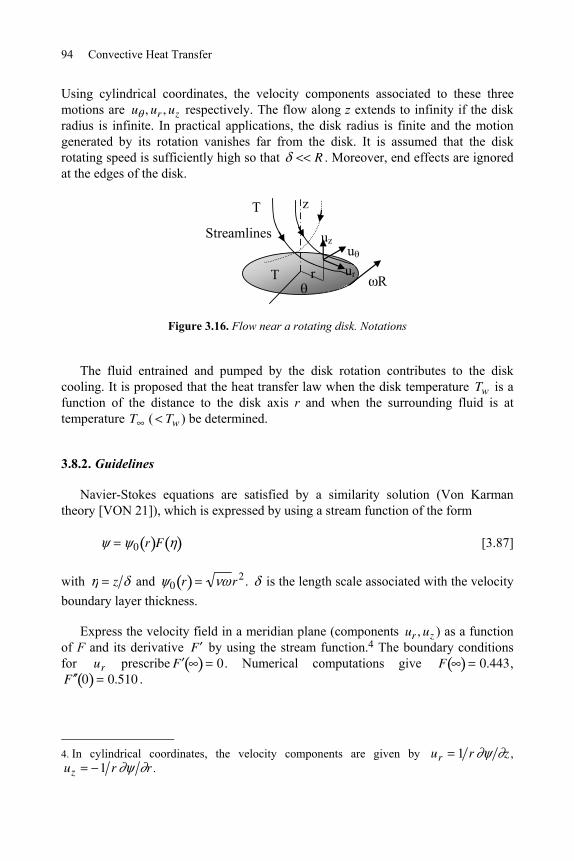
94 Convective Heat Transfer
Using cylindrical coordinates, the velocity components associated to these three motions are u , ur , uz respectively. The flow along z extends to infinity if the disk radius is infinite. In practical applications, the disk radius is finite and the motion generated by its rotation vanishes far from the disk. It is assumed that the disk rotating speed is sufficiently high so that R . Moreover, end effects are ignored at the edges of the disk.
uz
z
ur RrT
T
uStreamlines
Figure 3.16. Flow near a rotating disk. Notations
The fluid entrained and pumped by the disk rotation contributes to the disk cooling. It is proposed that the heat transfer law when the disk temperature Tw is a function of the distance to the disk axis r and when the surrounding fluid is at temperature T ( Tw ) be determined.
3.8.2. Guidelines
Navier-Stokes equations are satisfied by a similarity solution (Von Karman theory [VON 21]), which is expressed by using a stream function of the form
0 r F [3.87]
with z and 0 r r2 . is the length scale associated with the velocity boundary layer thickness.
Express the velocity field in a meridian plane (components ur , uz ) as a function of F and its derivative F by using the stream function.4 The boundary conditions for ur prescribe F 0. Numerical computations give F 0.443, F 0 0.510 .
4. In cylindrical coordinates, the velocity components are given by ur 1 r z , uz 1 r r .
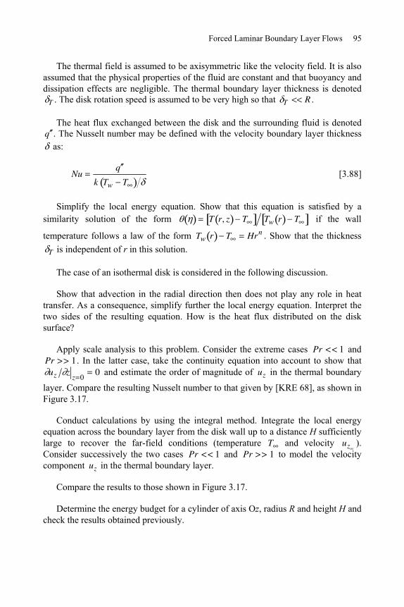
Forced Laminar Boundary Layer Flows 95
The thermal field is assumed to be axisymmetric like the velocity field. It is also assumed that the physical properties of the fluid are constant and that buoyancy and dissipation effects are negligible. The thermal boundary layer thickness is denoted
T . The disk rotation speed is assumed to be very high so that T R .
The heat flux exchanged between the disk and the surrounding fluid is denoted q . The Nusselt number may be defined with the velocity boundary layer thickness
as:
Nuq
k Tw T [3.88]
Simplify the local energy equation. Show that this equation is satisfied by a similarity solution of the form T r, z T Tw r T if the wall
temperature follows a law of the form Tw r T Hrn . Show that the thickness
T is independent of r in this solution.
The case of an isothermal disk is considered in the following discussion.
Show that advection in the radial direction then does not play any role in heat transfer. As a consequence, simplify further the local energy equation. Interpret the two sides of the resulting equation. How is the heat flux distributed on the disk surface?
Apply scale analysis to this problem. Consider the extreme cases Pr << 1 and Pr >> 1. In the latter case, take the continuity equation into account to show that uz z
z 00 and estimate the order of magnitude of uz in the thermal boundary
layer. Compare the resulting Nusselt number to that given by [KRE 68], as shown in Figure 3.17.
Conduct calculations by using the integral method. Integrate the local energy equation across the boundary layer from the disk wall up to a distance H sufficiently large to recover the far-field conditions (temperature T and velocity uz ). Consider successively the two cases Pr << 1 and Pr >> 1 to model the velocity component uz in the thermal boundary layer.
Compare the results to those shown in Figure 3.17.
Determine the energy budget for a cylinder of axis Oz, radius R and height H and check the results obtained previously.
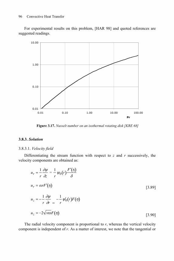
96 Convective Heat Transfer
For experimental results on this problem, [HAR 98] and quoted references are suggested readings.
0.01
0.10
1.00
10.00
0.01 0.10 1.00 10.00 100.00
Pr
Figure 3.17. Nusselt number on an isothermal rotating disk [KRE 68]
3.8.3. Solution
3.8.3.1. Velocity field
Differentiating the stream function with respect to z and r successively, the velocity components are obtained as:
ur1
r z =
1
r0 r
F
ur rF [3.89]
uz1
r r =
1
r0 r F
uz 2 F [3.90]
The radial velocity component is proportional to r, whereas the vertical velocity component is independent of r. As a matter of interest, we note that the tangential or
Forced Laminar Boundary Layer Flows 97
azimuthal velocity component is obviously also proportional to r. The three velocity components depend on z through the function F .
3.8.3.2. Similarity solution for the thermal field
Assuming that the temperature field is axisymmetric, advection does not play any role in the azimuthal direction. The energy equation is written with cylindrical coordinates and simplifies into:
urT
ruz
T
z
1
r rr
T
r
2T
z 2
The first term in the bracket represents radial diffusion and is of the order of R2 with Tw T . The second term represents diffusion in the normal
direction and is of the order of T2 . Since it was assumed that T R , the
energy equation is governed by the second term and further simplifies into:
urT
ruz
T
z
2T
z 2 [3.91]
We try a solution of the form:
T r, z T
Tw r T with Tw r T Hrn
Introducing expressions [3.89] and [3.90] and the transformation of variables defined above for the temperature, equation [3.91] becomes:
rF nHr n 1 2 F Hr n Hr n
Simplifying by Hrn , it is found that satisfies the second-order ordinary differential equation:
Pr 2F nF 0 [3.92]
The boundary conditions are:
0 1 , 0
98 Convective Heat Transfer
It can be concluded that equation [3.92] has, in effect, a similarity solution since the variable r has been eliminated in this equation. According to the form of the dimensionless temperature , the thermal boundary layer thickness is independent of r, like .
3.8.3.3. Uniform disk temperature
When the disk is isothermal, n = 0 in [3.92]. The energy equation further simplifies into:
2PrF 0 [3.93]
The thermal field is independent of r and advection in the radial direction does not play any role in heat transfer.
Equivalently, equation [3.91] simplifies into:
uzT
z
2T
z2 [3.94]
Thermal equilibrium is maintained near the disk by the fluid motion in the z-direction, which is opposite to thermal diffusion in the same direction.
The temperature gradient T
z z 0
Tp T0 is independent of r, as well as
the heat flux. Note that 0 is a function of the Prandtl number, since Pr is present in [3.93].
3.8.3.3.1. Scale analysis
The thermal boundary layer is characterized by its thickness T . The temperature gradient T z is estimated by T , as it is in the general case. The Nusselt
number, defined by Nuq
k Tw T with q k
T
z z 0
, is estimated by:
NuT
[3.95]
Pr << 1
As the fluid diffuses heat better than momentum, it is expected that the thermal boundary layer is thicker than the velocity boundary layer (Figure 3.18). The order
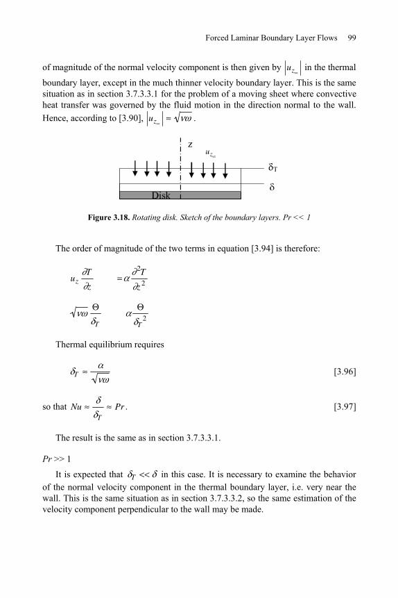
Forced Laminar Boundary Layer Flows 99
of magnitude of the normal velocity component is then given by uz in the thermal
boundary layer, except in the much thinner velocity boundary layer. This is the same situation as in section 3.7.3.3.1 for the problem of a moving sheet where convective heat transfer was governed by the fluid motion in the direction normal to the wall. Hence, according to [3.90], uz .
Figure 3.18. Rotating disk. Sketch of the boundary layers. Pr << 1
The order of magnitude of the two terms in equation [3.94] is therefore:
uzT
z
2T
z 2
T
T
2
Thermal equilibrium requires
T
[3.96]
so that NuT
Pr .
[3.97]
The result is the same as in section 3.7.3.3.1.
Pr >> 1
It is expected that T in this case. It is necessary to examine the behavior of the normal velocity component in the thermal boundary layer, i.e. very near the wall. This is the same situation as in section 3.7.3.3.2, so the same estimation of the velocity component perpendicular to the wall may be made.
100 Convective Heat Transfer
The role of the corresponding fluid motion in heat transfer is, however, different. In the moving sheet problem, heat transfer was governed by longitudinal advection because the velocity and thermal boundary layer thicknesses varied with x. In the present situation, these thicknesses are independent of x, so radial advection does not play any role in heat transfer. Only forced convection in direction z contributes to heat transfer.
In the present axisymmetric flow, the continuity equation reads:
1
r rrur
uz
z0
On the disk, the radial velocity component is zero, whatever the distance r, owing to the no-slip condition. As a result, 1 r r rur z 0
0 and therefore
uz zz 0
0 .
A development in series of the velocity component uz near the disk wall gives:
u z z u z 0 uz z 0
z2uz
z20
z2
2...
The first two terms are zero; 2uz z2
0is estimated by uz
2 . The velocity
is estimated in the thermal boundary layer by setting z T in the above development. The numerical coefficient 1/2 is ignored in this order of magnitude calculation.
uz T
uz
2 T2 T
2
2
The ratio of the velocities uz T and uz is proportional to T2 2 (<< 1).
The order of magnitude of the two terms in equation [3.94] is the following:
advection along z T2
2T
diffusion along z T
2
Forced Laminar Boundary Layer Flows 101
The thickness T is deduced from equilibrium between the two phenomena
T1
Pr1 3 [3.98]
so that NuT
Pr1 3.
[3.99]
When comparing the results with those of the moving sheet problem, it is worth noting the different exponent of Pr in law [3.83] and the absence of Re in laws [3.97] and [3.99]. This is due to the fact that the boundary layer thicknesses are uniform in the present problem and to the definition of the Nusselt number.
3.8.3.3.2. Calculation by integral method
Equation [3.94] is integrated over z between 0 and H (>> T ):
uzT
zdz0
H2T
z 20
HT
z 0 [3.100]
Pr << 1
The approximation uz uz is again adopted in the whole thermal boundary layer. The velocity component uz deviates from its asymptotic value only in the velocity boundary layer, which is much thinner than the thermal boundary layer, so that the error due to this approximation is expected to be very weak. uz may be taken out of the integral, which becomes:
uzT
zdz0
H uz T Tw
The right-hand side of [3.100] is also q C p . Equation [3.100] may be written
uz T Twq
C p [3.101]
Using the definition of the Nusselt number [3.88] and result [3.101], we find that:
Nuuz
102 Convective Heat Transfer
Numerical computations associated with the similarity solution have given F 0.443. According to [3.90], uz 0.886 , so that:
Nu 0.886Pr [3.102]
Pr >> 1
The calculation of the normal velocity component near the wall performed above
by scale analysis suggests the model for uz z to be uz z2uz
z20
z2
2.
Taking [3.90] into account, we obtain
2uz
z 2
uz2
F
F
so thatuz
uz
b2
2 [3.103]
with bF 0
F =
0.51
0.443 = 1.15.
The temperature profile is modeled, by using [3.36], as:
T(z) T
Tw T( ) 1
3
2
3
2 with
z
T
.
Equation [3.100] becomes:
uz b2
2
Tw T
T
3
22 1 dz0
H Tw T
T0
is kept as integration variable and we set Y T . The equation to be solved is then:
uz bY 3
22 2 1 d0
1
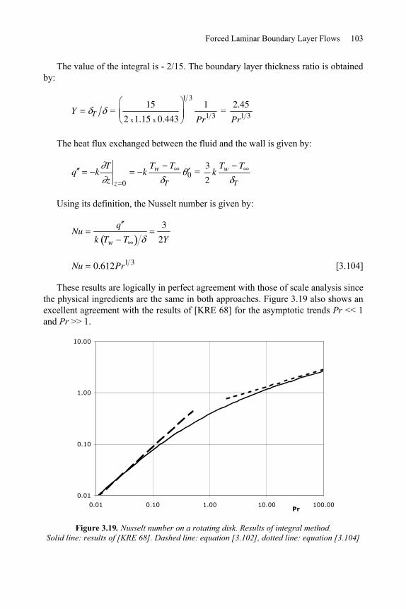
Forced Laminar Boundary Layer Flows 103
The value of the integral is - 2/15. The boundary layer thickness ratio is obtained by:
Y T = 15
2 x1.15 x 0.443
1 31
Pr1 3 =
2.45
Pr1 3
The heat flux exchanged between the fluid and the wall is given by:
q kT
z z 0
kTw T
T0 =
3
2k
Tw T
T
Using its definition, the Nusselt number is given by:
Nuq
k Tw T
3
2Y
Nu 0.612Pr1 3 [3.104]
These results are logically in perfect agreement with those of scale analysis since the physical ingredients are the same in both approaches. Figure 3.19 also shows an excellent agreement with the results of [KRE 68] for the asymptotic trends Pr << 1 and Pr >> 1.
0.01
0.10
1.00
10.00
0.01 0.10 1.00 10.00 100.00Pr
Figure 3.19. Nusselt number on a rotating disk. Results of integral method. Solid line: results of [KRE 68]. Dashed line: equation [3.102], dotted line: equation [3.104]
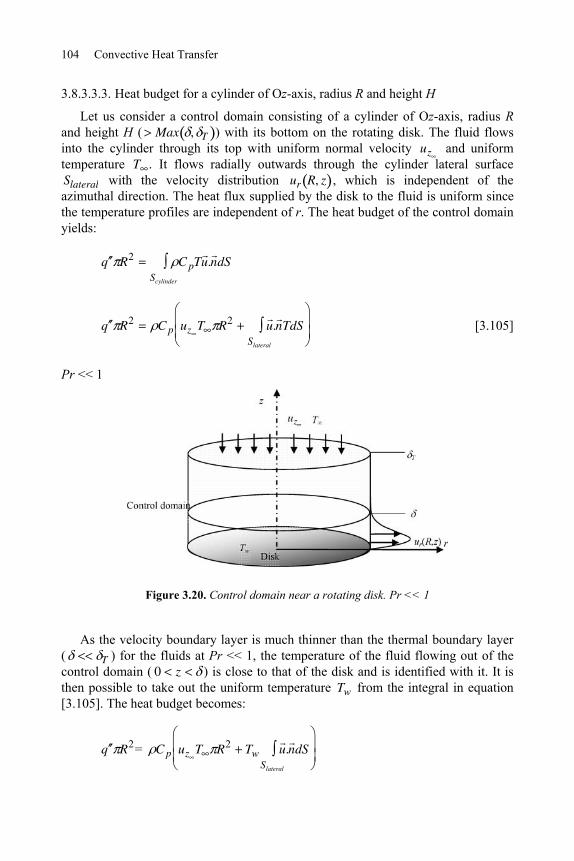
104 Convective Heat Transfer
3.8.3.3.3. Heat budget for a cylinder of Oz-axis, radius R and height H
Let us consider a control domain consisting of a cylinder of Oz-axis, radius R and height H ( Max , T ) with its bottom on the rotating disk. The fluid flows into the cylinder through its top with uniform normal velocity uz and uniform temperature T . It flows radially outwards through the cylinder lateral surface Slateral with the velocity distribution ur R, z , which is independent of the azimuthal direction. The heat flux supplied by the disk to the fluid is uniform since the temperature profiles are independent of r. The heat budget of the control domain yields:
q R2 C pTu .n dSScylinder
q R2 C p uz T R2 u .n TdSSlateral
[3.105]
Pr << 1
Figure 3.20. Control domain near a rotating disk. Pr << 1
As the velocity boundary layer is much thinner than the thermal boundary layer ( T ) for the fluids at Pr << 1, the temperature of the fluid flowing out of the control domain ( 0 z ) is close to that of the disk and is identified with it. It is then possible to take out the uniform temperature Tw from the integral in equation [3.105]. The heat budget becomes:
q R2= C p uz T R2 Tw u .n dSSlateral
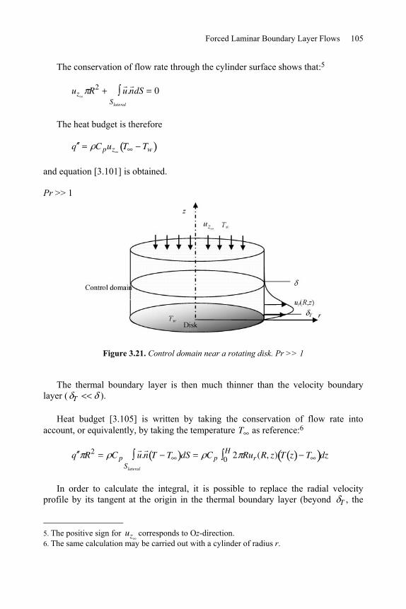
Forced Laminar Boundary Layer Flows 105
The conservation of flow rate through the cylinder surface shows that:5
uz R2 u .n dSSlateral
0
The heat budget is therefore
q C puz T Tw
and equation [3.101] is obtained.
Pr >> 1
Figure 3.21. Control domain near a rotating disk. Pr >> 1
The thermal boundary layer is then much thinner than the velocity boundary layer ( T ).
Heat budget [3.105] is written by taking the conservation of flow rate into account, or equivalently, by taking the temperature T as reference:6
q R2 C p u .n T T dSSlateral
C p 2 Rur (R, z) T z T dz0H
In order to calculate the integral, it is possible to replace the radial velocity profile by its tangent at the origin in the thermal boundary layer (beyond T , the
5. The positive sign for uz corresponds to Oz-direction. 6. The same calculation may be carried out with a cylinder of radius r.
106 Convective Heat Transfer
contribution to the energy flow rate is zero and T ), so that, according to [3.89], the approximation is ur R, z RF 0 z .
The temperature profile is modeled, as it is in section 3.8.3.3.2, by:
T(z) T
Tw T( ) 1
3
2
3
2 with
z
T
Substituting into the energy budget equation, we find
C p 2 R2F 0 Tw Tz
13
2
3
2dz0
T kTw T
T0 R2
or, setting Y T and simplifying the equation
2 F 0Y 3 2 13
2
3
2d0
10
The value of the integral is 1/10. F 0 0.510 0 3 2 . We find Y2.45
Pr1 3
and result [3.104] is obtained.
3.9. Thermal loss in a duct
3.9.1. Description of the problem
Oil is flowing with bulk velocity U and temperature T0 in fully developed laminar regime in a channel of spacing e delimited by two parallel plates. The length Lz of the plates in the spanwise direction is sufficiently long so that the flow is considered as two-dimensional. The walls are perfectly insulated, except on a small surface Sl of dimensions l x Lz on one of the walls (Figure 3.22). It is assumed that the local wall temperature is uniform and equal to Tw0 on Sl . It is proposed that the total heat transfer rate lost by oil on Sl and the wall temperature distribution Tw x in the region downstream from the heat sink are calculated.
Data: e = 10 cm, l = 10 cm, Lz = 1 m, U cm s-1 T0 = 80°C, Tw0 = 20°C.
The physical properties of oil are given in Table 3.6.
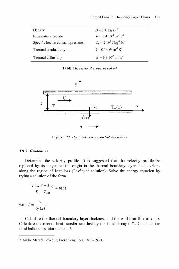
Forced Laminar Boundary Layer Flows 107
Density = 850 kg m-3
Kinematic viscosity = 0.4 10-4 m-2 s-1
Specific heat at constant pressure Cp = 2 103 J kg-1 K-1
Thermal conductivity k = 0.14 W m-1 K-1
Thermal diffusivity = 0.8 10-7 m2 s-1
Table 3.6. Physical properties of oil
Figure 3.22. Heat sink in a parallel-plate channel
3.9.2. Guidelines
Determine the velocity profile. It is suggested that the velocity profile be replaced by its tangent at the origin in the thermal boundary layer that develops along the region of heat loss (Lévêque7 solution). Solve the energy equation by trying a solution of the form
T(x, y) Tw0
T0 Tw0
( )
with y
T (x).
Calculate the thermal boundary layer thickness and the wall heat flux at x = l. Calculate the overall heat transfer rate lost by the fluid through Sl . Calculate the fluid bulk temperature for x = l. 7. André Marcel Lévêque, French engineer, 1896–1930.
108 Convective Heat Transfer
Propose a method to calculate Tw x for x > l. It is suggested that two functions be superposed in order to satisfy the condition of zero wall heat flux for x > l.
3.9.3. Solution
3.9.3.1. Velocity distribution in the channel
In a hydraulically fully developed regime, the solution to Navier-Stokes equations gives the following velocity profile (see Chapter 2, equation [2.13])
u( )
U6 1
[3.106]
with y e . Note that the origin of ordinates y has been chosen in the plane containing Sl and that y is normalized by the overall channel spacing.
The velocity profile is replaced by its tangent at the origin:
u( )
U6 6
y
e
3.9.3.2. Lévêque solution to the energy equation
A thermal boundary layer is developing on the part of the wall lacking insulating material. The energy equation is written in this region with the usual boundary layer approximations
6Uy
e
T
x
2T
y2
or using the transformation of variables y
T (x),
T(x, y) Tw0
T0 Tw0
( )
6U T
e2 t
T T2
Introducing the Péclet number Pe Ue and the dimensionless variables
x* x e , T* x*
T x e , the energy equation becomes:
6Pe T*2
T* 2
[3.107]
Forced Laminar Boundary Layer Flows 109
Separating the functions of x* and the functions of , we find that:
6Pe T*2
T* Constant
[3.108]
The constant is arbitrary and for sake of convenience, we choose Constant = 3.
Equation [3.108] is easily integrated as
T* x* 3
2Pex*
1 3
[3.109]
where the condition T* 0 0 has been accounted for. Equation [3.107] then
becomes
3 2
which is integrated by two successive quadratures
3expA [3.110]
30 expA z dz
[3.111]
with 3
0
1 1,12exp
Az dz
.
Equations [3.109] and [3.111] constitute the Lévêque solution of the problem of a thermal boundary layer developing in a plane channel in a hydraulically fully developed flow. The temperature profile is plotted in Figure 3.23.
3.9.3.3. Thermal boundary layer thickness
Equation [3.109] gives the characteristic thermal boundary layer thickness:
T* l* 3
2Pel*
1 3
with
l* l
e
Pe0.01 x 0,1
0.8 x10 712500
l* 1
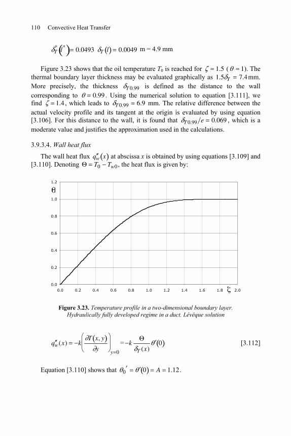
110 Convective Heat Transfer
T* l* 0.0493
T l 0.0049 m = 4.9 mm
Figure 3.23 shows that the oil temperature T0 is reached for 1.5 ( 1). The thermal boundary layer thickness may be evaluated graphically as 1.5 T 7.4mm. More precisely, the thickness T 0.99 is defined as the distance to the wall corresponding to 0.99 . Using the numerical solution to equation [3.111], we find 1.4 , which leads to T 0.99 6.9 mm. The relative difference between the actual velocity profile and its tangent at the origin is evaluated by using equation [3.106]. For this distance to the wall, it is found that T 0.99 e 0.069 , which is a moderate value and justifies the approximation used in the calculations.
3.9.3.4. Wall heat flux
The wall heat flux q w x at abscissa x is obtained by using equations [3.109] and [3.110]. Denoting T0 Tw0 , the heat flux is given by:
0.0
0.2
0.4
0.6
0.8
1.0
1.2
0.0 0.2 0.4 0.6 0.8 1.0 1.2 1.4 1.6 1.8 2.0
Figure 3.23. Temperature profile in a two-dimensional boundary layer. Hydraulically fully developed regime in a duct. Lévêque solution
q w(x) kT x, y
y y 0
= kT (x)
0
[3.112]
Equation [3.110] shows that 0 0 A 1.12 .
Forced Laminar Boundary Layer Flows 111
According to [3.109], T x e3
2Pex*
1 3
Introducing the reference heat flux q 0 k e , we obtain:
q w(x*)
q 0
2
3
1 3
APe
x*
1 3
0.978Pe
x*
1 3
[3.113]
q 0 0.1460
0.184 W m-2 with x* l* 1, q w(l) = 1906 W m-2
The overall heat transfer rate q(x) Lz lost by the fluid on the length x per transverse unit is obtained by integrating the local heat flux q w(x) over x
q(x) Lz q 0x (x1)dx1 q 0e 0.978 Pe x1
* 1/ 3
0x*
dx1*
q(x) Lz3
20.978k Pe1 3 x
e
2 3
Bk Pe1 3 x
e
2 3
[3.114]
with B = 1.467.
For x = l, we obtain
q(l) Lz3
2q w l l
and finally, q(l) Lz 286 W m-1.
3.9.3.5. Fluid bulk temperature in the region downstream from the heat sink
The energy budget is written for a control domain delimited by an upstream cross-section, a cross-section of abscissa x (0 < x < l), and the channel walls. Using the fluid bulk temperature Tm(x) in the cross-section of abscissa x, the energy equation yields:
q(x) Lz C pUe T0 Tm x [3.115]
In the cross-section corresponding to the downstream end of Sl (x = l), we obtain:
q(l) Lz C pUe T0 Tm l
112 Convective Heat Transfer
The energy budget gives T0 Tm l 0.17 °C. The fluid bulk temperature Tm0 Tm l does not vary any more in the downstream region of the channel since the walls are perfectly insulated for x l .
3.9.3.6. Distribution of wall temperature downstream from the heat sink
Since the walls are perfectly insulated for x l , the temperature field must satisfy the condition of zero wall-heat flux in this region. As a consequence, the temperature profile is modified and the wall temperature increases for x l . It is convenient to represent these changes as resulting from a second boundary layer embedded in the first one and developing from the abscissa x = l (Figure 3.24).
The temperature profile for x l may then be considered as resulting from the superposition of two profiles corresponding to the two boundary layers CL1 and CL2 that are developing on the wall from the abscissas x = 0 and x = l respectively.
3.9.3.6.1. Superposition of two Lévêque solutions
An approximate solution consists of superposing Lévêque-type solutions, as presented in section 3.9.3.2. This is not an exact solution since the wall temperature is not uniform in the region downstream from the heat sink, contrary to the condition prescribed for 0 < x < l in CL1.
Solution for CL1:
T 1 (x, y) Tw0 ( 1) with 1y
T1(x) [3.116]
Solution for CL2:
T 2 (x, y) Tw2(x)
Tw2(x)( 2 ) with 2
y
T 2 (x) [3.117]
where the function is the Lévêque solution, as given by [3.111].
According to [3.109], the Lévêque solution also gives T1 x e3
2Pe
x
e
1 3
or,
changing the origin of x for CL2, T 2 x e3
2Pe
x l
e
1 3
.
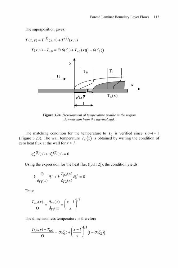
Forced Laminar Boundary Layer Flows 113
The superposition gives:
T (x, y) T 1 (x, y) T 2 (x, y)
T(x, y) Tw0 ( 1) Tw2(x) 1 ( 2 )
Figure 3.24. Development of temperature profile in the region downstream from the thermal sink
The matching condition for the temperature to T0 is verified since ( ) 1 (Figure 3.23). The wall temperature Tw x is obtained by writing the condition of zero heat flux at the wall for x > l.
q w1 (x) q w
2 (x) 0
Using the expression for the heat flux ([3.112]), the condition yields:
kT1(x)
0 kTp2(x)
T 2(x)0 0
Thus:
Tw2(x) T 2(x)
T1(x)
x l
x
1 3
The dimensionless temperature is therefore
T(x, y) Tw0 ( 1)x l
x
1 3
1 ( 2 )
114 Convective Heat Transfer
and, since (0) 0 , the corresponding wall temperature is
Tw(x) Tw0 1l
x
1 3
[3.118]
The wall temperature grows rapidly and tends to the fluid temperature of the channel central region (Figure 3.25). The initial temperature difference is recovered within about 10% for x/l = 4.
3.9.3.6.2. Integral method
It is also possible to apply the principle of superposition in freeing the function T 2 x , whereas it had a prescribed form in the previous approach. We then
superpose a Lévêque solution [3.116], corresponding to CL1 and a function T 2 (x, y) corresponding to CL2. For this latter function, it is possible to use the formalism of equation [3.117]; however, the function corresponding to the shape of the temperature profile, denoted ( ), has to be modeled. Moreover, the function T 2 x has to be determined simultaneously with Tw2(x). We therefore
must write two equations in two unknown functions. For ( ), it is suggested that a polynomial be used, matching to 0 for 2 1 .
The conservation of enthalpy flow rate through a cross-section downstream from the heat sink yields:
C p0e u(x, y) T (x, y) T0 dy C pU Tm0 T0 e [3.119]
Introducing the decomposition T (x, y) T 1 (x, y) T 2 (x, y) into [3.119], the calculation of the integral of the left-hand side may be performed in two parts. According to [3.114] and [3.115], the Lévêque solution gives:
2 31 1 3
0 00 ( , ) ( , )ep p m
xC u x y T x y T dy C Ue T T x Bk Pe
e
Using a linear approximation of the velocity profile together with equation [3.117] (the shape of the function (2) will be specified later), the profile T 2 (x, y) gives the following calculation
C p0e u(x, y)T 2 (x, y)dy C pU 6
y
e0e Tw2(x) 1 2
2 T 2 x d 2
6
ea C pUTw2 (x) T 2 x
2
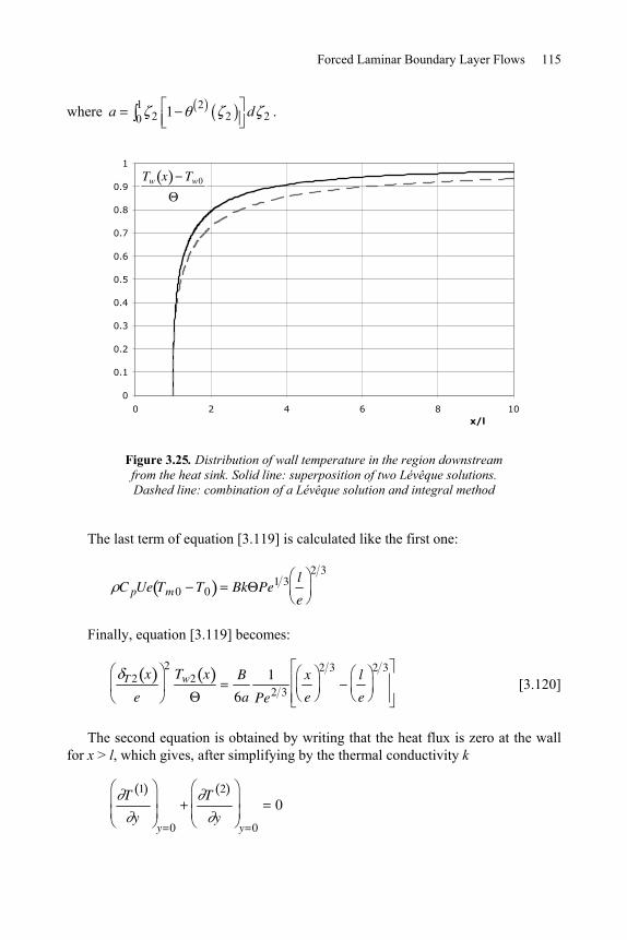
Forced Laminar Boundary Layer Flows 115
where 1 22 2 20 1a d .
0
0.1
0.2
0.3
0.4
0.5
0.6
0.7
0.8
0.9
1
0 2 4 6 8 10x/l
Tw x Tw0
Figure 3.25. Distribution of wall temperature in the region downstream from the heat sink. Solid line: superposition of two Lévêque solutions. Dashed line: combination of a Lévêque solution and integral method
The last term of equation [3.119] is calculated like the first one:
C pUe Tm0 T0 Bk Pe1 3 l
e
2 3
Finally, equation [3.119] becomes:
T 2 x
e
2Tw2 x B
6a
1
Pe2 3
x
e
2 3l
e
2 3
[3.120]
The second equation is obtained by writing that the heat flux is zero at the wall for x > l, which gives, after simplifying by the thermal conductivity k
T 1
yy 0
T 2
yy 0
0
116 Convective Heat Transfer
T1(x)0
Tw2 (x)
T 2 (x)
d (2)
d 22 0
0
or denoting 02 d (2)
d 22 0
Tw2(x) 0
02
T 2(x)
T1(x)
[3.121]
Substituting [3.121] in [3.120] and using law [3.109] for the thickness T1 x of the boundary layer CL1 as a function of x, we obtain the thickness of the boundary layer CL2
T 2 x
eC
l e
Pe
1 3x
l
x
l
1 3 1 3
[3.122]
with C3
20
2
0
B
6a
1 3
02
4a
1 3
and the law giving Tw2(x)
Tw2(x)D 1
l
x
2 3 1 3
[3.123]
with D 0
02
C
3
2
1 3
It is worth recalling that 0 1.12 in the Lévêque solution. It is now possible to specify the shape of the temperature profile ( ). Choosing a form similar to
Forced Laminar Boundary Layer Flows 117
[3.35] ( 2 ( 2)3
22
23
2), we obtain 0
2 3
2, a
1
10, and the following
laws:
T 2 x
e1.554
l e
Pe
1 3x
l
x
l
1 3 1 3
[3.124]
Tw(x) Tw0 Tw2(x)1.013 1
l
x
2 3 1 3
[3.125]
Equation [3.125] is plotted in Figure 3.25. The curve exhibits a moderate deviation relative to the solution in section 3.9.3.6.1. The relative difference decreases from 12% for the smallest values of x/l to 3% for the highest values. It is consistent to find the highest relative deviation in the region of the fastest variations in wall temperature since the actual thermal condition in this region is far from that used in the Lévêque theory, namely uniform wall temperature.
Note that the approximation that consists of replacing the velocity profile by its tangent at the origin becomes less and less appropriate in the downstream direction. It is possible to improve the calculation by using the actual velocity profile and the integral method.
3.10. Temperature profile for heat transfer with blowing
3.10.1. Description of the problem
Let us consider convective heat transfer near a porous wall at temperature Tw higher than that of the fluid in the far region T . A transverse flow is generated through the wall with the local velocity v0.
How does the energy equation simplify on the wall (y = 0+)? Study the sign of 2T y2 and T y across the boundary layer and show that the temperature
profile presents a point of inflexion at some distance to the wall.

118 Convective Heat Transfer
3.10.2. Solution
The energy equation in a boundary layer [3.15] simplifies on the wall into
v0T
yy 0
2T
y2y 0
[3.126]
where the no-slip condition at the wall (u = 0) and the blowing condition have been taken into account. In the classical situation where the wall is impermeable
( v0 0 ), 2T
y2y 0
0 , which leads to (0) 0 in the conditions prescribed for the
temperature profile in the integral method (section 3.3.2). This is not the case in the present situation.
Accounting for heating conditions, it is expected that the heat flux is directed
from the wall towards the fluid, say T
yy 0
0 .
Since v0 0 for blowing, we deduce from [3.126] that 2T
y2y 0
0 . The
conductive heat flux supplied by the wall to the fluid ( q 0) is proportional to T y and therefore increases with y near the wall. Far from the wall, the
conductive heat flux tends to 0 (the fluid temperature tends to T ); it then exhibits a
maximum at a point M, where 2T
y2y yM
0 . Hence, the temperature profile
presents a point of inflexion in M. The situation is shown in Figure 3.26.
x
y
Tp
T
M T(x,y)
v0
u
Figure 3.26. Boundary layer with blowing through a porous wall. Temperature profile
Chapter 4
Forced Convection Around Obstacles
4.1. Description of the flow
This chapter is devoted to heat transfer on bodies immersed in a stream. We consider a solid characterized by the length scale L placed in a stream characterized by the reference velocity U, which is generally the velocity far upstream from the obstacle (several times the length L in practice). If the solid is heated to a temperature T different from that of the fluid, heat transfer occurs in the vicinity of the solid surface and in the downstream wake. The thermal field depends strongly on the flow field, which is characterized by the Reynolds number Re = UL .
We first distinguish the flows at Re << 1 and Re >> 1. The first type of flow is present in limited domains of application (sedimentation, thermo-anemometry). These creeping flows are governed by viscous effects.
Flows of the second type (Re >> 1) are more often encountered in practical applications. These flows are characterized by thin velocity and thermal boundary layers in the upstream part of the obstacle. A particular streamline ends at a stagnation point A located in front of the obstacle. Boundary layers originate in the stagnation region and then grow in the downstream direction up to the trailing edge for streamlined bodies (Figure 4.1). A velocity wake (velocity defect) and a thermal wake (temperature excess when the solid is heated) develop behind the obstacle. The wake region follows the development of the boundary layers when the obstacle is well profiled.
When the obstacle is not well profiled (bluff body), the flow separates at some distance downstream from the stagnation point, where the pressure would have
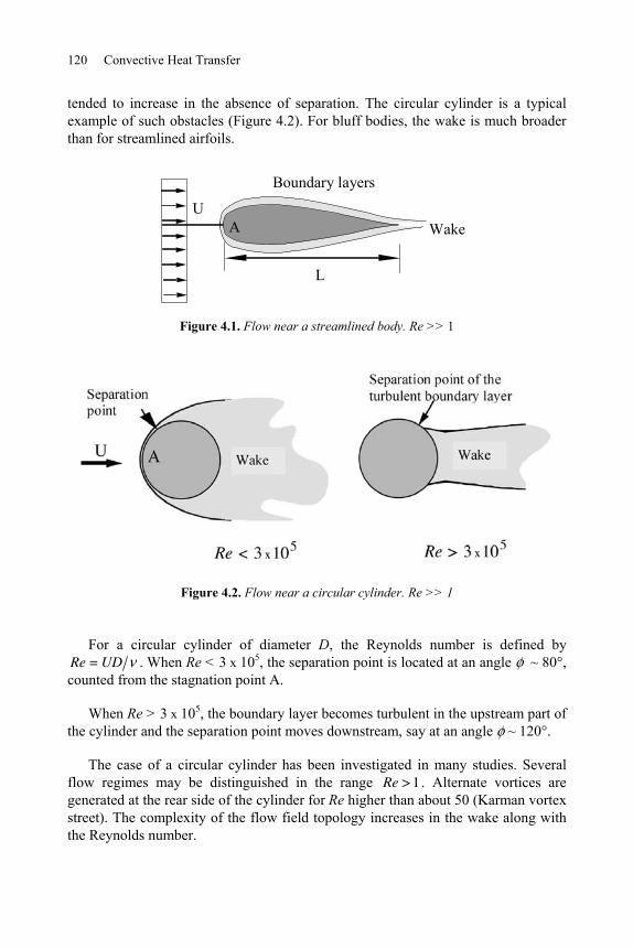
120 Convective Heat Transfer
tended to increase in the absence of separation. The circular cylinder is a typical example of such obstacles (Figure 4.2). For bluff bodies, the wake is much broader than for streamlined airfoils.
L
Boundary layers
U WakeA
Figure 4.1. Flow near a streamlined body. Re >> 1
Figure 4.2. Flow near a circular cylinder. Re >> 1
For a circular cylinder of diameter D, the Reynolds number is defined by Re = UD . When Re < 3 x 10⁵, the separation point is located at an angle ~ 80°, counted from the stagnation point A.
When Re > 3 x 10⁵, the boundary layer becomes turbulent in the upstream part of the cylinder and the separation point moves downstream, say at an angle ~ 120°.
The case of a circular cylinder has been investigated in many studies. Several flow regimes may be distinguished in the range Re >1 . Alternate vortices are generated at the rear side of the cylinder for Re higher than about 50 (Karman vortex street). The complexity of the flow field topology increases in the wake along with the Reynolds number.
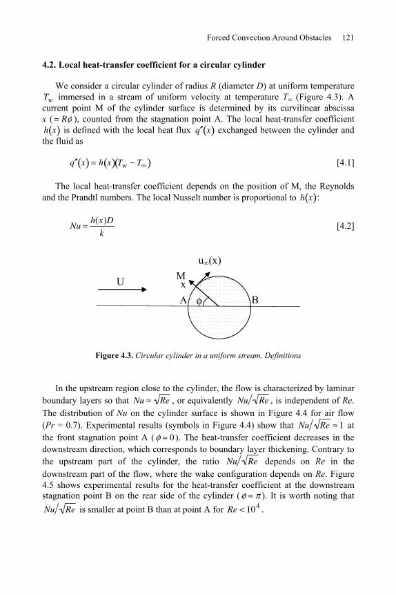
Forced Convection Around Obstacles 121
4.2. Local heat-transfer coefficient for a circular cylinder
We consider a circular cylinder of radius R (diameter D) at uniform temperature Tw immersed in a stream of uniform velocity at temperature T (Figure 4.3). A current point M of the cylinder surface is determined by its curvilinear abscissa x ( R ), counted from the stagnation point A. The local heat-transfer coefficient h x is defined with the local heat flux q x exchanged between the cylinder and the fluid as
q x h x Tw T [4.1]
The local heat-transfer coefficient depends on the position of M, the Reynolds and the Prandtl numbers. The local Nusselt number is proportional to h x :
Nuh(x)D
k [4.2]
BA
U
u (x)
xM
Figure 4.3. Circular cylinder in a uniform stream. Definitions
In the upstream region close to the cylinder, the flow is characterized by laminar boundary layers so that Nu Re , or equivalently Nu Re , is independent of Re. The distribution of Nu on the cylinder surface is shown in Figure 4.4 for air flow (Pr = 0.7). Experimental results (symbols in Figure 4.4) show that Nu Re 1 at the front stagnation point A ( 0 ). The heat-transfer coefficient decreases in the downstream direction, which corresponds to boundary layer thickening. Contrary to the upstream part of the cylinder, the ratio Nu Re depends on Re in the downstream part of the flow, where the wake configuration depends on Re. Figure 4.5 shows experimental results for the heat-transfer coefficient at the downstream stagnation point B on the rear side of the cylinder ( ). It is worth noting that Nu Re is smaller at point B than at point A for Re 104 .
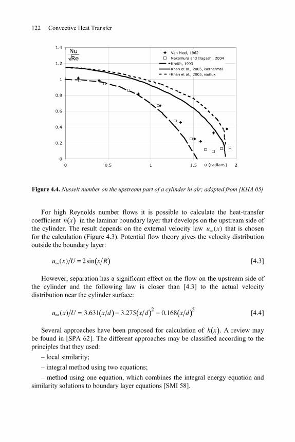
122 Convective Heat Transfer
Figure 4.4. Nusselt number on the upstream part of a cylinder in air; adapted from [KHA 05]
For high Reynolds number flows it is possible to calculate the heat-transfer coefficient h x in the laminar boundary layer that develops on the upstream side of the cylinder. The result depends on the external velocity law u (x) that is chosen for the calculation (Figure 4.3). Potential flow theory gives the velocity distribution outside the boundary layer:
u (x) U 2sin x R [4.3]
However, separation has a significant effect on the flow on the upstream side of the cylinder and the following law is closer than [4.3] to the actual velocity distribution near the cylinder surface:
u (x) U 3.631 x d 3.275 x d 2 0.168 x d 5 [4.4]
Several approaches have been proposed for calculation of h x . A review may be found in SPA 62 . The different approaches may be classified according to the principles that they used:
– local similarity; – integral method using two equations; – method using one equation, which combines the integral energy equation and
similarity solutions to boundary layer equations [SMI 58].
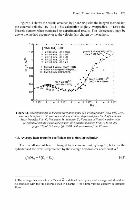
Forced Convection Around Obstacles 123
Figure 4.4 shows the results obtained by [KHA 05] with the integral method and the external velocity law [4.3]. This calculation slightly overpredicts ( 15%) the Nusselt number when compared to experimental results. This discrepancy may be due to the method accuracy or to the velocity law chosen by the authors.
Figure 4.5. Nusselt number at the rear stagnation point of a cylinder in air [NAK 04]. CHF: constant heat flux, CWT: constant wall temperature. Reprinted from Int. J. of Heat and Mass Transfer, Vol. 47, NAKAMURA H., IGARASHI T., Variation of Nusselt number with
flow regimes behind a circular cylinder for Reynolds numbers from 70 to 30,000, pages 5169-5173, copyright 2004, with permission from Elsevier
4.3. Average heat-transfer coefficient for a circular cylinder
The overall rate of heat exchanged by transverse unit, q q Lz , between the cylinder and the flow is represented by the average heat-transfer coefficient h 1
q DLz h Tw T [4.5]
1. The average heat-transfer coefficient h is defined here by a spatial average and should not be confused with the time average used in Chapter 7 for a time-varying quantity in turbulent flows.
124 Convective Heat Transfer
or in dimensionless form
Nuh D
k
q DLz
k Tw T D [4.6]
Nu depends on Re and Pr. Many correlations are available in the literature. For example, Churchill and Bernstein [CHU 77a] recommend:
Nu 0.30.62Re1 2Pr1 3
1+ 0.4 Pr 2 3 1 41
Re
282 000
5 8 4 5
[4.7]
for 0.2 < Pe = Re Pr.
Nu , Re, Pr are calculated with the fluid physical properties at the film temperature Tf Tw T 2 . For uniform wall heat flux, equation [4.7] may be used with the temperature averaged on the cylinder perimeter. [BEJ 95] indicates that equation [4.7] underestimates the Nusselt number by up to 20% when compared to experimental results in the range 7 x 10⁴ < Re < 4 x 10⁵.
The law of Collis and Williams [COL 59] may be applied to low Reynolds number air flows and consequently to thermo-anemometry applications
Nu A BRen T T fa
[4.8]
where the coefficients n, A, B and a are given in Table 4.1.
0.02 < Re < 44 44 < Re < 140
n 0.45 0.51
A 0.24 0
B 0.56 0.48
a -0.17 -0.17
Table 4.1. Coefficients of the Collis and Williams law [COL 59]
The fluid physical properties are evaluated at Tf = Tw T 2 .
Nakamura and Igarashi [NAK 04] give the results in Figure 4.6.
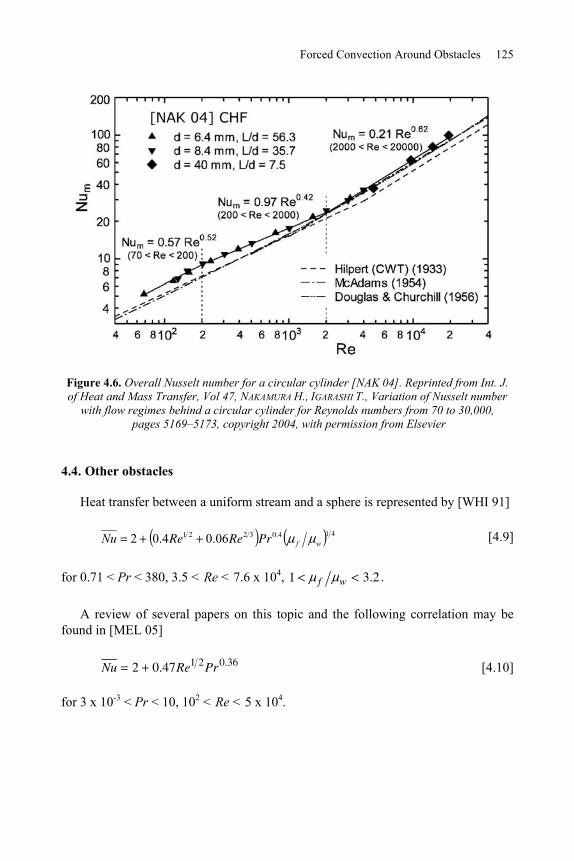
Forced Convection Around Obstacles 125
Figure 4.6. Overall Nusselt number for a circular cylinder [NAK 04]. Reprinted from Int. J. of Heat and Mass Transfer, Vol 47, NAKAMURA H., IGARASHI T., Variation of Nusselt number
with flow regimes behind a circular cylinder for Reynolds numbers from 70 to 30,000, pages 5169–5173, copyright 2004, with permission from Elsevier
4.4. Other obstacles
Heat transfer between a uniform stream and a sphere is represented by [WHI 91]
413206.04.02 wPrReRe fNu 0.421 [4.9]
for 0.71 < Pr < 380, 3.5 < Re < 7.6 x 10⁴, 1 f w 3.2 .
A review of several papers on this topic and the following correlation may be found in [MEL 05]
Nu 2 0.47Re1 2Pr0.36 [4.10]
for 3 x 10⁻³ < Pr < 10, 102 < Re < 5 x 10⁴.
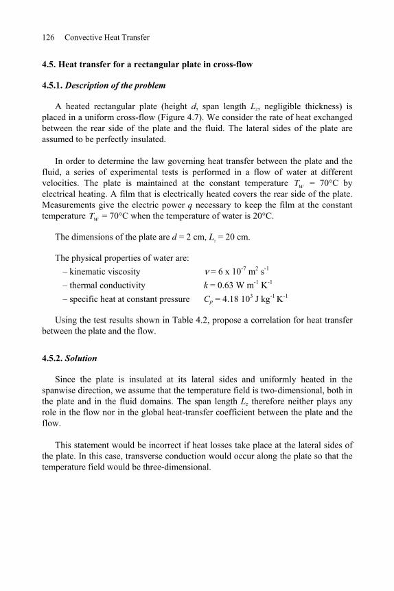
126 Convective Heat Transfer
4.5. Heat transfer for a rectangular plate in cross-flow
4.5.1. Description of the problem
A heated rectangular plate (height d, span length Lz, negligible thickness) is placed in a uniform cross-flow (Figure 4.7). We consider the rate of heat exchanged between the rear side of the plate and the fluid. The lateral sides of the plate are assumed to be perfectly insulated.
In order to determine the law governing heat transfer between the plate and the
fluid, a series of experimental tests is performed in a flow of water at different velocities. The plate is maintained at the constant temperature Tw = 70°C by electrical heating. A film that is electrically heated covers the rear side of the plate. Measurements give the electric power q necessary to keep the film at the constant temperature Tw = 70°C when the temperature of water is 20°C.
The dimensions of the plate are d = 2 cm, Lz = 20 cm.
The physical properties of water are: – kinematic viscosity = 6 x 10⁻⁷ m2 s-1
– thermal conductivity k = 0.63 W m-1 K-1 – specific heat at constant pressure Cp = 4.18 103 J kg-1 K-1
Using the test results shown in Table 4.2, propose a correlation for heat transfer between the plate and the flow.
4.5.2. Solution
Since the plate is insulated at its lateral sides and uniformly heated in the spanwise direction, we assume that the temperature field is two-dimensional, both in the plate and in the fluid domains. The span length Lz therefore neither plays any role in the flow nor in the global heat-transfer coefficient between the plate and the flow.
This statement would be incorrect if heat losses take place at the lateral sides of
the plate. In this case, transverse conduction would occur along the plate so that the temperature field would be three-dimensional.
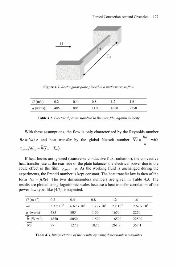
Forced Convection Around Obstacles 127
U d
Lz
Figure 4.7. Rectangular plate placed in a uniform cross-flow
U (m/s) 0.2 0.4 0.8 1.2 1.6
q (watts) 485 805 1150 1650 2250
Table 4.2. Electrical power supplied to the rear film against velocity
With these assumptions, the flow is only characterized by the Reynolds number
Re = Ud and heat transfer by the global Nusselt number Nu =h d
k with
qconv dLz h Tw T .
If heat losses are ignored (transverse conductive flux, radiation), the convective heat transfer rate at the rear side of the plate balances the electrical power due to the Joule effect in the film, qconv q . As the working fluid is unchanged during the experiments, the Prandtl number is kept constant. The heat transfer law is then of the form Nu = f(Re) . The two dimensionless numbers are given in Table 4.3. The results are plotted using logarithmic scales because a heat transfer correlation of the power-law type, like [4.7], is expected.
U (m s-1) 0.2 0.4 0.8 1.2 1.6
Re 3.3 x 10³ 6.67 x 10³ 1.33 x 10³ 2 x 10⁴ 2.67 x 10⁴
q (watts) 485 805 1150 1650 2250
h (W m-2) 4850 8050 11500 16500 22500
Nu 77 127.8 182.5 261.9 357.1
Table 4.3. Interpretation of the results by using dimensionless variables
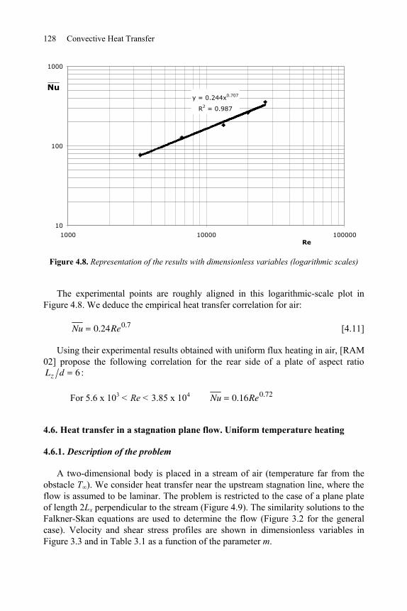
128 Convective Heat Transfer
y = 0.244x0.707
R2 = 0.987
10
100
1000
1000 10000 100000Re
Nu
Figure 4.8. Representation of the results with dimensionless variables (logarithmic scales)
The experimental points are roughly aligned in this logarithmic-scale plot in Figure 4.8. We deduce the empirical heat transfer correlation for air:
Nu 0.24Re0.7 [4.11]
Using their experimental results obtained with uniform flux heating in air, [RAM 02] propose the following correlation for the rear side of a plate of aspect ratio Lz d 6 :
For 5.6 x 10³ < Re < 3.85 x 10⁴ Nu 0.16Re0.72
4.6. Heat transfer in a stagnation plane flow. Uniform temperature heating
4.6.1. Description of the problem
A two-dimensional body is placed in a stream of air (temperature far from the obstacle T ). We consider heat transfer near the upstream stagnation line, where the flow is assumed to be laminar. The problem is restricted to the case of a plane plate of length 2Lx perpendicular to the stream (Figure 4.9). The similarity solutions to the Falkner-Skan equations are used to determine the flow (Figure 3.2 for the general case). Velocity and shear stress profiles are shown in dimensionless variables in Figure 3.3 and in Table 3.1 as a function of the parameter m.
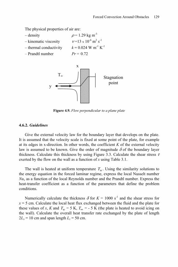
Forced Convection Around Obstacles 129
The physical properties of air are: – density = 1.29 kg m-3 – kinematic viscosity =13 x 10-6 m2 s-1
– thermal conductivity k = 0.024 W m-1 K-1 – Prandtl number Pr = 0.72
Stagnation point
x
y
T
Figure 4.9. Flow perpendicular to a plane plate
4.6.2. Guidelines
Give the external velocity law for the boundary layer that develops on the plate. It is assumed that the velocity scale is fixed at some point of the plate, for example at its edges in x-direction. In other words, the coefficient K of the external velocity law is assumed to be known. Give the order of magnitude of the boundary layer thickness. Calculate this thickness by using Figure 3.3. Calculate the shear stress exerted by the flow on the wall as a function of x using Table 3.1.
The wall is heated at uniform temperature Tw . Using the similarity solutions to the energy equation in the forced laminar regime, express the local Nusselt number Nux as a function of the local Reynolds number and the Prandtl number. Express the heat-transfer coefficient as a function of the parameters that define the problem conditions.
Numerically calculate the thickness for K = 1000 s-1 and the shear stress for x = 5 cm. Calculate the local heat flux exchanged between the fluid and the plate for these values of x, K and Tw = 5 K, T = - 5 K (the plate is heated to avoid icing on the wall). Calculate the overall heat transfer rate exchanged by the plate of length 2Lx = 10 cm and span length Lz = 50 cm.
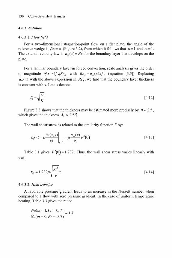
130 Convective Heat Transfer
4.6.3. Solution
4.6.3.1. Flow field
For a two-dimensional stagnation-point flow on a flat plate, the angle of the reference wedge is (Figure 3.2), from which it follows that 1 and m 1. The external velocity law is u (x) Kx for the boundary layer that develops on the plate.
For a laminar boundary layer in forced convection, scale analysis gives the order of magnitude x 1 Rex with Rex u (x)x (equation [3.5]). Replacing u (x) with the above expression in Rex , we find that the boundary layer thickness is constant with x. Let us denote:
1 K [4.12]
Figure 3.3 shows that the thickness may be estimated more precisely by 2.5 , which gives the thickness 2 2.5 1.
The wall shear stress is related to the similarity function F by:
0(x)u(x, y)
yy 0
u (x)
1
F 0 [4.13]
Table 3.1 gives F 0 1.232 . Thus, the wall shear stress varies linearly with x as:
0 1.232K 3
x [4.14]
4.6.3.2. Heat transfer
A favorable pressure gradient leads to an increase in the Nusselt number when compared to a flow with zero pressure gradient. In the case of uniform temperature heating, Table 3.3 gives the ratio:
Nu(m 1, Pr 0, 7)
Nu(m 0, Pr 0, 7)1.7
Forced Convection Around Obstacles 131
Using the heat transfer law for a plane plate (equation [3.24]), the local Nusselt number is obtained as:
Nux 1.7 x 0.332Rex1 2Pr1 3 0.564Rex
1 2Pr1 3 [4.15]
The heat-transfer coefficient is therefore constant with x:
h 0.564kK
Pr1 3 [4.16]
With the data given above, we calculate for x = 5 cm:
2 0.28 mm , 0 9.1 Nm 2 , h 106.5 Wm 2K 1
The local heat flux is q h T Tw =1065 Wm 2 and the total heat transfer rate exchanged between the fluid and the plate is q q 2LxLz = 53 W.
4.7. Heat transfer in a stagnation plane flow. Step-wise heating at uniform flux
4.7.1. Description of the problem
We again consider the problem in section 4.6 with, however, two important differences. The plate heating is now started at a location downstream from the stagnation point (Figure 4.10). Moreover, the plate is heated at uniform flux instead of uniform temperature. The plate is unheated on the length x0 so that a thermal boundary layer develops beyond this starting length and is therefore embedded in the velocity boundary layer that starts at the leading edge of the plate. The plate is heated at uniform flux q 0 for x x0 . The wall temperature is then T for x < x0 and increases further downstream.
The unknown wall temperature is denoted Tw x in the heated region. Let us denote x Tw x T .
We plan to determine the heat transfer law between the wall and the fluid for x x0 .
132 Convective Heat Transfer
Stagnation point
x
y
T
x0
Figure 4.10. Step-wise heating at uniform flux
4.7.2. Guidelines
The problem is restricted to the initial region of the thermal boundary layer. Propose a velocity profile u(x,y) inside the thermal boundary layer by using Figure 3.3 and replace the actual velocity profile near the wall by its tangent at the origin.
Use the integral energy equation applied to a boundary layer flow. Assume that the heat flux q 0 is independent of x and determine the rate of enthalpy convected through a section perpendicular to the wall as a function of x.
It is suggested that the following polynomial be used to represent the temperature profile in the thermal boundary layer of thickness T x
T(x, y) T
Tw (x) T( ) 1
3
2
1
23 [4.17]
with = y T x , 0 1.
Determine a relation between (x) and T x (take the boundary condition in x = x0 into account).
Use the profile given by equation [4.17] in the relation between the heat flux and the temperature gradient at the wall and find a second equation between (x) and
T x .
Combine these equations to calculate (x) and T x . Determine the heat transfer law giving the local Nusselt number Nux as a function of Rex and the ratio x0 x . Verify that when x0 = 0, the heat transfer law is close to that issuing from the similarity solution.
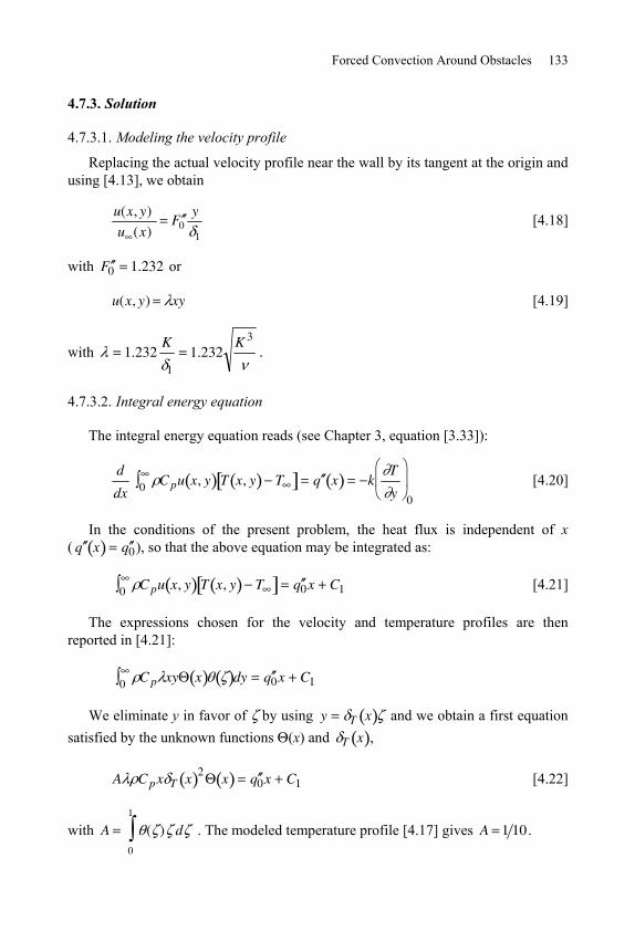
Forced Convection Around Obstacles 133
4.7.3. Solution
4.7.3.1. Modeling the velocity profile
Replacing the actual velocity profile near the wall by its tangent at the origin and using [4.13], we obtain
u(x, y)u (x)
F 0y
1
[4.18]
with F 0 1.232 or
u(x, y) xy [4.19]
with 1.232K
11.232
K 3.
4.7.3.2. Integral energy equation
The integral energy equation reads (see Chapter 3, equation [3.33]):
d
dx 0 C pu x, y T x, y T q x kT
y 0
[4.20]
In the conditions of the present problem, the heat flux is independent of x ( q x q 0), so that the above equation may be integrated as:
0 C pu x, y T x, y T q 0x C1 [4.21]
The expressions chosen for the velocity and temperature profiles are then reported in [4.21]:
0 C p xy x dy q 0x C1
We eliminate y in favor of by using y T x and we obtain a first equation satisfied by the unknown functions (x) and T x ,
A C px T x 2 x q 0x C1 [4.22]
with A ( ) d0
1
. The modeled temperature profile [4.17] gives A 1 10 .
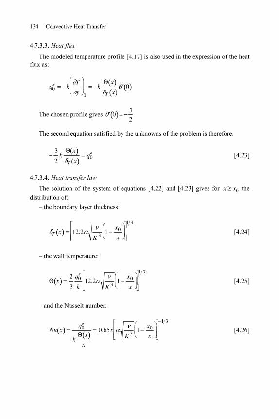
134 Convective Heat Transfer
4.7.3.3. Heat flux
The modeled temperature profile [4.17] is also used in the expression of the heat flux as:
q 0 kT
y 0
kx
T x0
The chosen profile gives 032
.
The second equation satisfied by the unknowns of the problem is therefore:
3
2k
x
T xq 0 [4.23]
4.7.3.4. Heat transfer law
The solution of the system of equations [4.22] and [4.23] gives for x x0 the distribution of:
– the boundary layer thickness:
T x 12.2K 3
1x0
x
1 3
[4.24]
– the wall temperature:
x2
3
q 0k
12.2K 3
1x0
x
1 3
[4.25]
– and the Nusselt number:
Nu xq 0
kx
x
0.65xK 3
1x0
x
1 3
[4.26]
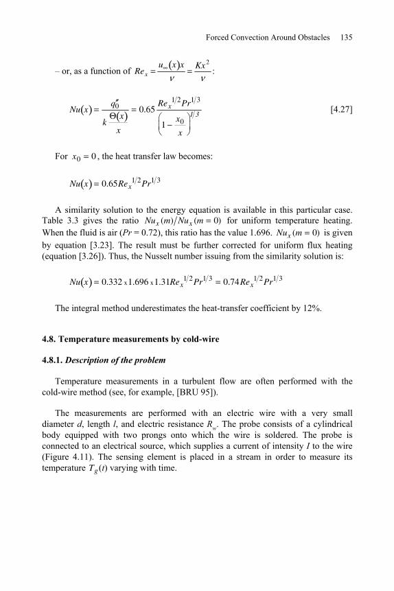
Forced Convection Around Obstacles 135
– or, as a function of Rex
u x x Kx2
:
Nu xq 0
kx
x
0.65Rex
1 2Pr1 3
1x0
x
1 3 [4.27]
For x0 0 , the heat transfer law becomes:
Nu x 0.65Rex1 2Pr1 3
A similarity solution to the energy equation is available in this particular case. Table 3.3 gives the ratio Nux (m) Nux (m 0) for uniform temperature heating. When the fluid is air (Pr = 0.72), this ratio has the value 1.696. Nux (m 0)
is given by equation [3.23]. The result must be further corrected for uniform flux heating (equation [3.26]). Thus, the Nusselt number issuing from the similarity solution is:
Nu x 0.332 x1.696 x1.31Rex1 2Pr1 3 0.74Rex
1 2Pr1 3
The integral method underestimates the heat-transfer coefficient by 12%.
4.8. Temperature measurements by cold-wire
4.8.1. Description of the problem
Temperature measurements in a turbulent flow are often performed with the cold-wire method (see, for example, [BRU 95]).
The measurements are performed with an electric wire with a very small diameter d, length l, and electric resistance Rw. The probe consists of a cylindrical body equipped with two prongs onto which the wire is soldered. The probe is connected to an electrical source, which supplies a current of intensity I to the wire (Figure 4.11). The sensing element is placed in a stream in order to measure its temperature Tg(t) varying with time.
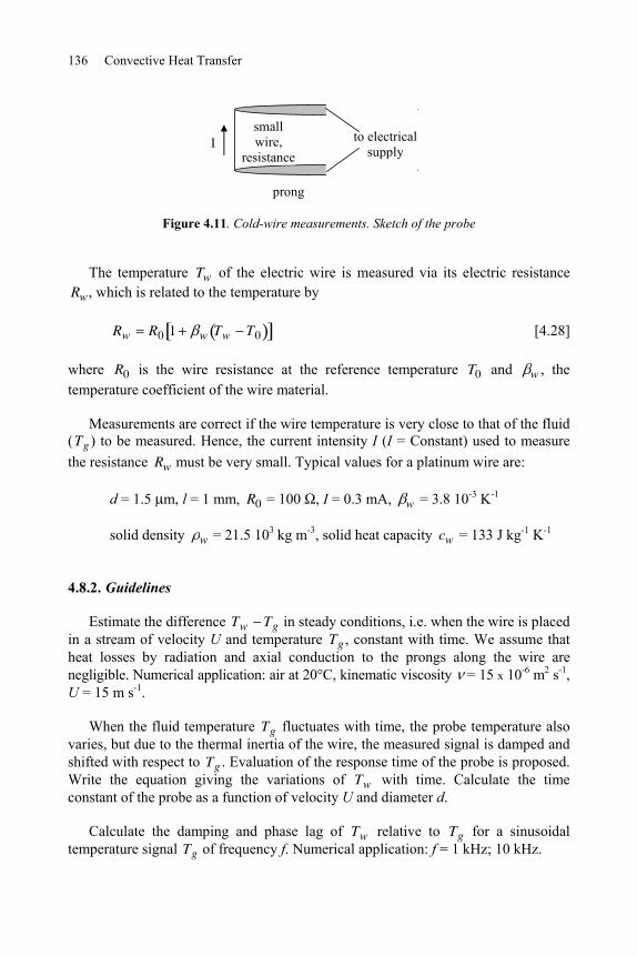
136 Convective Heat Transfer
to electrical supply
prong
small wire,
resistance I
Figure 4.11. Cold-wire measurements. Sketch of the probe
The temperature Tw of the electric wire is measured via its electric resistance Rw , which is related to the temperature by
Rw R0 1 w Tw T0 [4.28]
where R0 is the wire resistance at the reference temperature T0 and w , the temperature coefficient of the wire material.
Measurements are correct if the wire temperature is very close to that of the fluid (Tg) to be measured. Hence, the current intensity I (I = Constant) used to measure the resistance Rw must be very small. Typical values for a platinum wire are:
d = 1.5 m l = 1 mm, R0 = 100 , I = 0.3 mA, w = 3.8 10-3 K-1
solid density w = 21.5 103 kg m-3, solid heat capacity cw = 133 J kg-1 K-1
4.8.2. Guidelines
Estimate the difference Tw Tg in steady conditions, i.e. when the wire is placed in a stream of velocity U and temperature Tg , constant with time. We assume that heat losses by radiation and axial conduction to the prongs along the wire are negligible. Numerical application: air at 20°C, kinematic viscosity = 15 x 10-6 m2 s-1, U = 15 m s-1.
When the fluid temperature Tg fluctuates with time, the probe temperature also varies, but due to the thermal inertia of the wire, the measured signal is damped and shifted with respect to Tg . Evaluation of the response time of the probe is proposed. Write the equation giving the variations of Tw with time. Calculate the time constant of the probe as a function of velocity U and diameter d.
Calculate the damping and phase lag of Tw relative to Tg for a sinusoidal temperature signal Tg of frequency f. Numerical application: f = 1 kHz; 10 kHz.
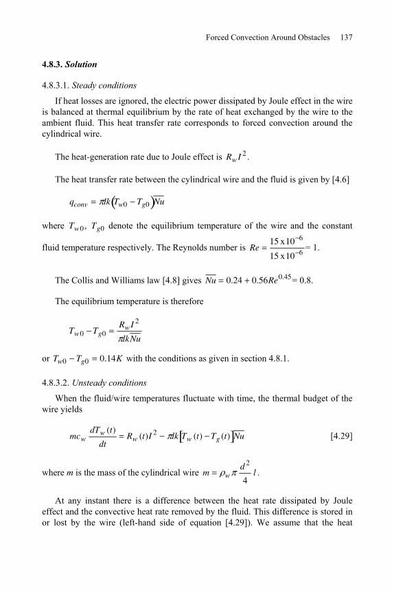
Forced Convection Around Obstacles 137
4.8.3. Solution
4.8.3.1. Steady conditions
If heat losses are ignored, the electric power dissipated by Joule effect in the wire is balanced at thermal equilibrium by the rate of heat exchanged by the wire to the ambient fluid. This heat transfer rate corresponds to forced convection around the cylindrical wire.
The heat-generation rate due to Joule effect is Rw I 2 .
The heat transfer rate between the cylindrical wire and the fluid is given by [4.6]
qconv lk Tw0 Tg0 Nu
where Tw0, Tg0 denote the equilibrium temperature of the wire and the constant
fluid temperature respectively. The Reynolds number is Re15 x10 6
15 x10 6= 1.
The Collis and Williams law [4.8] gives Nu 0.24 0.56Re0.45= 0.8.
The equilibrium temperature is therefore
Tw0 Tg0Rw I 2
lkNu
or Tw0 Tg0 0.14K with the conditions as given in section 4.8.1.
4.8.3.2. Unsteady conditions
When the fluid/wire temperatures fluctuate with time, the thermal budget of the wire yields
mcwdTw (t)
dtRw (t)I 2 lk Tw (t) Tg (t) Nu [4.29]
where m is the mass of the cylindrical wire m wd 2
4l .
At any instant there is a difference between the heat rate dissipated by Joule effect and the convective heat rate removed by the fluid. This difference is stored in or lost by the wire (left-hand side of equation [4.29]). We assume that the heat
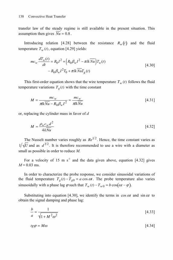
138 Convective Heat Transfer
transfer law of the steady regime is still available in the present situation. This assumption then gives Nu 0.8 .
Introducing relation [4.28] between the resistance Rw t and the fluid temperature Tw (t) , equation [4.29] yields:
2 20 0
20 0
( )( )
( )
ww w w
w g
dT tmc R I R I lk Nu T t
dtR I T lk NuT t
[4.30]
This first-order equation shows that the wire temperature Tw (t) follows the fluid temperature variations Tg (t) with the time constant
Mmcw
lkNu R0 w I 2
mcw
lkNu [4.31]
or, replacing the cylinder mass in favor of d
M wcw d 2
4kNu [4.32]
The Nusselt number varies roughly as Re1 2 . Hence, the time constant varies as 1 U and as d 3 2 . It is therefore recommended to use a wire with a diameter as small as possible in order to reduce M.
For a velocity of 15 m s-1 and the data given above, equation [4.32] gives M = 0.03 ms.
In order to characterize the probe response, we consider sinusoidal variations of the fluid temperature Tg (t) Tg0 a cos t . The probe temperature also varies sinusoidally with a phase lag such that Tw (t) Tw 0 b cos t .
Substituting into equation [4.30], we identify the terms in cos t and sin t to obtain the signal damping and phase lag:
b
a
1
1 M 2 2 [4.33]
tg M [4.34]
Forced Convection Around Obstacles 139
With the data of the problem, we find for:
f = 1 kHz, b a = 0.98, = 10.7°
f = 10 kHz, b a = 0.47, = 62°
With a cold-wire of 1 m, it is then possible to measure temperature fluctuations of the order of 1 kHz. In order to perform measurements at higher frequency, a wire of smaller diameter must be used (0.6 m).

This page intentionally left blank
Chapter 5
External Natural Convection
5.1. Introduction
Natural convection corresponds to situations where the fluid is set in motion by buoyancy forces due to density variations. These density variations may result from heat transfer inside the fluid or between the fluid and heated or cooled solid walls. It may also result from mass transfer when the fluid is a multi-component mixture.
Contrary to the situations described in the previous chapters, natural convection flows are not due to external mechanical power, but solely to heat or mass transfer, which leads to density variations inside the fluid. It is worth underlining two main properties of natural convection flows:
– there is a strong coupling between the flow and heat transfer. In natural convection problems, it is not possible to calculate successively the velocity field, then the temperature field, as it is in forced convection when the fluid properties are considered as constant. The two fields must be calculated simultaneously, which makes the problems of natural convection rather difficult;
– buoyancy forces are generally weak so that the characteristic velocities are small compared to those which are found in forced convection. As a result, natural convection flows are mostly laminar. However, laminar-turbulent transition may occur like in forced convection.
Natural convection is very often encountered in many practical situations (cooling of electrical or electronic components, solar energy, domestic heating, etc.).
142 Convective Heat Transfer
5.2. Boussinesq model1
The relevant fundamental equations are those of fluid mechanics [1.2] and [1.6] and heat transfer [1.8] of the general type. Simplifying these equations is, however, possible in most applications and the resulting equations constitute the Boussinesq model. This model is available for moderate density variations (typically for relative variations within about 10%). The assumptions are the following:
– the variations of density are considered as linear against temperature T. Using an arbitrary reference state defined by p , , T (these variables are linked by the fluid state equation), density variations are given by:
T T [5.1]
where is the coefficient of thermal expansion at constant pressure;
– density variations are ignored in the continuity equation, which keeps the usual expression:
div u 0 [5.2]
– density variations are also negligible at first order in the inertia term of momentum equation [1.6] so that is replaced by in this term;
– in this chapter, the longitudinal axis Ox is chosen along the ascending vertical axis and we introduce the modified pressure: p* p gx . After decomposing pressure and accounting for the above assumptions, the momentum equation reads:
du
dt
1gradp* T T g u [5.3]
– velocities being weak, the term dp dt and the dissipation D are ignored with respect to the convection term in the energy equation. Without any heat source or sink, we then consider the following equation [1.10] instead of [1.8]:
dT
dtT [5.4]
5.3. Dimensionless numbers. Scale analysis
Let us consider a situation involving only one length scale L along the vertical axis and a temperature scale as in forced convection, this is a characteristic
1. Joseph Valentin Boussinesq, French mathematician and physicist, 1842–1929.
External Natural Convection 143
temperature difference between a solid and the surrounding fluid for a given problem). Normalizing the equations by using reference scales shows that two dimensionless numbers are relevant to natural convection flows:
– the Prandtl number Pr = , like in forced convection;
– the Grashof number Grg L3
2. [5.5]
The Rayleigh number is obtained by combining the two previous ones and is often more relevant than the Grashof number for characterizing natural convection:
Rag L3
Gr Pr [5.6]
Heat transfer is characterized in natural convection by correlations of the form:
Nu f Gr,Pr or, preferably, Nu f Ra,Pr .
In a very large reservoir, heat transfer is generally concentrated in boundary layers that develop near vertical walls. For a given temperature difference between a wall and the ambient fluid, scale analysis [BEJ 95] states the order of magnitude shown in Table 5.1 for:
– the velocity and thermal boundary layer thicknesses, and T respectively; – the characteristic velocity U in the direction parallel to the wall; – the Nusselt number.
The Rayleigh number is defined by using the distance x counted along the vertical axis from the wall leading edge (beginning of the boundary layers):
Raxg x 3
[5.7]
The local heat flux at abscissa x being q 0(x) , the Nusselt number is defined by:
Nuxq 0(x)
k x [5.8]
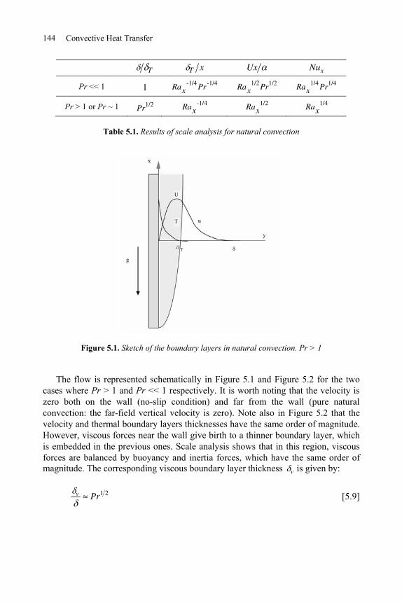
144 Convective Heat Transfer
T T x Ux Nux
Pr << 1 1 Rax-1/4 Pr -1/4 Rax
1/2Pr1/2 Rax1/4 Pr1/4
Pr > 1 or Pr ~ 1 Pr1/2 Rax-1/4 Rax
1/2 Rax1/4
Table 5.1. Results of scale analysis for natural convection
Figure 5.1. Sketch of the boundary layers in natural convection. Pr > 1
The flow is represented schematically in Figure 5.1 and Figure 5.2 for the two cases where Pr > 1 and Pr << 1 respectively. It is worth noting that the velocity is zero both on the wall (no-slip condition) and far from the wall (pure natural convection: the far-field vertical velocity is zero). Note also in Figure 5.2 that the velocity and thermal boundary layers thicknesses have the same order of magnitude. However, viscous forces near the wall give birth to a thinner boundary layer, which is embedded in the previous ones. Scale analysis shows that in this region, viscous forces are balanced by buoyancy and inertia forces, which have the same order of magnitude. The corresponding viscous boundary layer thickness v is given by:
v Pr1 2 [5.9]
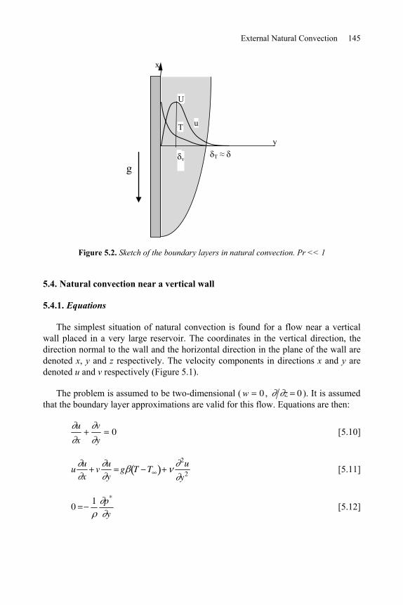
External Natural Convection 145
g
T u
U
y
x
v T
Figure 5.2. Sketch of the boundary layers in natural convection. Pr << 1
5.4. Natural convection near a vertical wall
5.4.1. Equations
The simplest situation of natural convection is found for a flow near a vertical wall placed in a very large reservoir. The coordinates in the vertical direction, the direction normal to the wall and the horizontal direction in the plane of the wall are denoted x, y and z respectively. The velocity components in directions x and y are denoted u and v respectively (Figure 5.1).
The problem is assumed to be two-dimensional ( w 0 , z 0 ). It is assumed that the boundary layer approximations are valid for this flow. Equations are then:
u
x
v
y0 [5.10]
uu
xv
u
yg T T
2u
y2 [5.11]
01 p*
y [5.12]
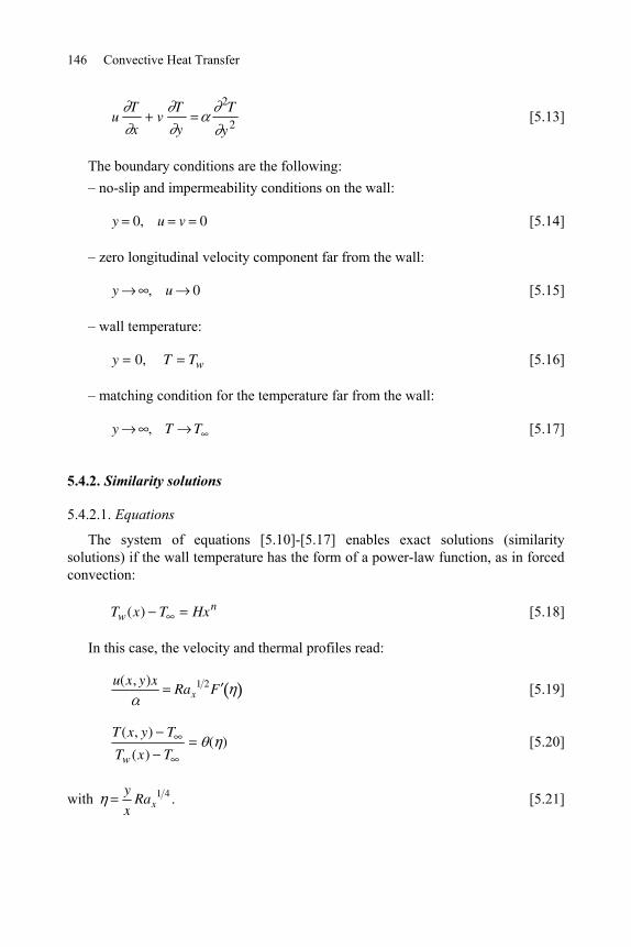
146 Convective Heat Transfer
uT
xv
T
y
2T
y2 [5.13]
The boundary conditions are the following: – no-slip and impermeability conditions on the wall:
y 0, u v 0 [5.14]
– zero longitudinal velocity component far from the wall:
y , u 0 [5.15]
– wall temperature:
y 0, T Tw [5.16]
– matching condition for the temperature far from the wall:
y , T T [5.17]
5.4.2. Similarity solutions
5.4.2.1. Equations
The system of equations [5.10]-[5.17] enables exact solutions (similarity solutions) if the wall temperature has the form of a power-law function, as in forced convection:
Tw(x) T Hxn [5.18]
In this case, the velocity and thermal profiles read:
u(x, y)xRax
1 2F [5.19]
T(x, y) T
Tw (x) T( ) [5.20]
with y
xRax
1 4 . [5.21]
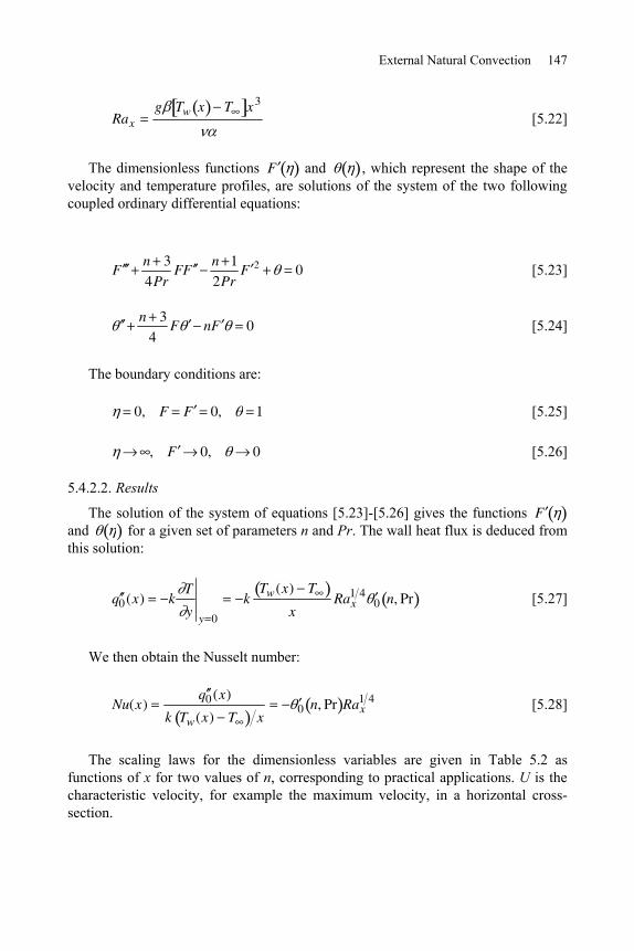
External Natural Convection 147
Raxg Tw x T x3
[5.22]
The dimensionless functions F and , which represent the shape of the velocity and temperature profiles, are solutions of the system of the two following coupled ordinary differential equations:
F n 34Pr
FF n 12Pr
F 2 0 [5.23]
n 34
F nF 0 [5.24]
The boundary conditions are:
0, F F 0, 1 [5.25]
, F 0, 0 [5.26]
5.4.2.2. Results
The solution of the system of equations [5.23]-[5.26] gives the functions F and for a given set of parameters n and Pr. The wall heat flux is deduced from this solution:
q 0(x) kT
y y 0
kTw(x) T
xRax
1 40 n, Pr [5.27]
We then obtain the Nusselt number:
Nu(x)q 0(x)
k Tw(x) T x0 n, Pr Rax
1 4 [5.28]
The scaling laws for the dimensionless variables are given in Table 5.2 as functions of x for two values of n, corresponding to practical applications. U is the characteristic velocity, for example the maximum velocity, in a horizontal cross-section.
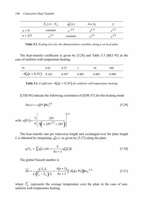
148 Convective Heat Transfer
Tw(x) T q 0(x) or T U
n 0 constant x -1 4 x1 4 x1 2 n 1 5 x1 5 constant x1 5 x3 5
Table 5.2. Scaling laws for the dimensionless variables along a vertical plate
The heat-transfer coefficient is given by [5.28] and Table 5.3 [BEJ 95] in the case of uniform wall-temperature heating.
Pr 0.01 0.72 1 10 100
0 n 0, Pr 0.162 0.387 0.401 0.465 0.490
Table 5.3. Coefficient 0 n 0, Pr for uniform wall temperature heating
[CEB 88] indicate the following correlation of [EDE 67] for this heating mode
Nu(x) a Pr Rax1 4 [5.29]
with a Pr3
4
2Pr
5 1 2Pr1 2 2Pr
1 4
.
The heat transfer rate per transverse length unit exchanged over the plate length L is obtained by integrating q 0(x) as given by [5.27] along the plate:
q Lz q 00L (x)dx
4
5n 3q 0 L L [5.30]
The global Nusselt number is
Nuq LzL
k Tw T L
4 n 1
5n 30 n, Pr RaL
1 4 [5.31]
where Tw represents the average temperature over the plate in the case of non-uniform wall temperature heating.
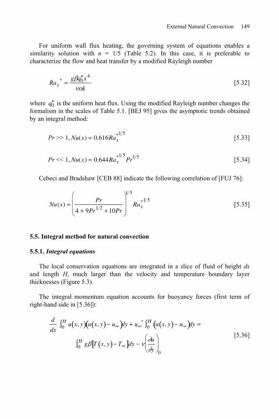
External Natural Convection 149
For uniform wall flux heating, the governing system of equations enables a similarity solution with n = 1/5 (Table 5.2). In this case, it is preferable to characterize the flow and heat transfer by a modified Rayleigh number
Rax* g q 0x4
k [5.32]
where q 0 is the uniform heat flux. Using the modified Rayleigh number changes the formalism in the scales of Table 5.1. [BEJ 95] gives the asymptotic trends obtained by an integral method:
Pr >> 1, Nu(x) 0.616Rax*1 5
[5.33]
Pr << 1, Nu(x) 0.644Rax*1 5
Pr1 5 [5.34]
Cebeci and Bradshaw [CEB 88] indicate the following correlation of [FUJ 76]:
Nu(x)Pr
4 9Pr1 2 10Pr
1 5
Rax*1 5
[5.35]
5.5. Integral method for natural convection
5.5.1. Integral equations
The local conservation equations are integrated in a slice of fluid of height dx and length H, much larger than the velocity and temperature boundary layer thicknesses (Figure 5.3).
The integral momentum equation accounts for buoyancy forces (first term of right-hand side in [5.36]):
d
dxu x, y u x, y u0
H dy u u x, y u0H dy
g0H T x, y T dy
u
y 0
[5.36]
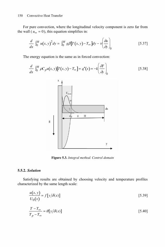
150 Convective Heat Transfer
For pure convection, where the longitudinal velocity component is zero far from the wall ( u 0), this equation simplifies in:
d
dxu x, y
20H dy g0
H T x, y T dyu
y 0 [5.37]
The energy equation is the same as in forced convection:
d
dx 0H C pu x, y T x, y T q x k
T
y 0
[5.38]
Figure 5.3. Integral method. Control domain
5.5.2. Solution
Satisfying results are obtained by choosing velocity and temperature profiles characterized by the same length scale:
u x, y
U0 xf y (x)
[5.39]
T T
T p Ty (x)
[5.40]
External Natural Convection 151
Contrary to the case of forced convection, the velocity scale U0 x is now unknown. Modeling the flow and thermal fields with only one length scale leads to a system of two equations in two unknowns x and U0 x . Accounting for the conditions that the functions f and must satisfy and choosing a polynomial form for these functions, we find the velocity and temperature shapes
f 1 2
[5.41]
1 2
[5.42]
with y (x) .
For a vertical plate heated at uniform temperature, [BUR 83] gives the following results
x
x3.94
C
RaxPr
1/ 4
[5.43]
Umax x x0.765
RaxPr
C
1/ 2
[5.44]
Nux 0.508RaxPr
C
1/ 2
[5.45]
Nu 0.677RaLPr
C
1/ 2
[5.46]
with
C20
21Pr [5.47]
These results are in good agreement with the similarity solutions.
152 Convective Heat Transfer
5.6. Correlations for external natural convection
Heat transfer correlations for external natural convection are shown in Table 5.4 in addition to the previous results. They are taken from [CHU 75], [FIS 50] and have been collected by [BEJ 95]. They take turbulence effects into account when the Grashof number based on the solid height becomes larger than a critical value. Typically, GrLcrit
109.
The fluid physical properties are taken at the film temperature 1 2 Tw T . The global Nusselt number Nu is based on the total heat transfer rate exchanged by the solid of surface S:
Nuq S
k Tw T L [5.48]
For a vertical plate heated at non-uniform temperature, Tw is the average temperature over the plate height. The reference length scale L is specified in the index of the Nusselt, Rayleigh and Grashof numbers and in the different cases is:
– the vertical plate height L; – the diameter d of a cylinder or a sphere; – a dimension calculated as the ratio of the surface to the perimeter in the case of
a horizontal plate A S p.
5.7. Mixed convection
The influence of buoyancy forces on a flow characterized by the velocity scale U is estimated by the Richardson number:
Rig L
U 2 =
buoyancy force per mass unit
inertia force per mass unit =
Gr
Re2
When Ri 1 , buoyancy forces are negligible (forced convection).
When Ri 1 , the flow and heat transfer are governed by buoyancy forces (pure natural convection). This is the case presented in the first sections of this chapter, where there is no velocity imposed to the fluid far from a heated solid (U = 0).
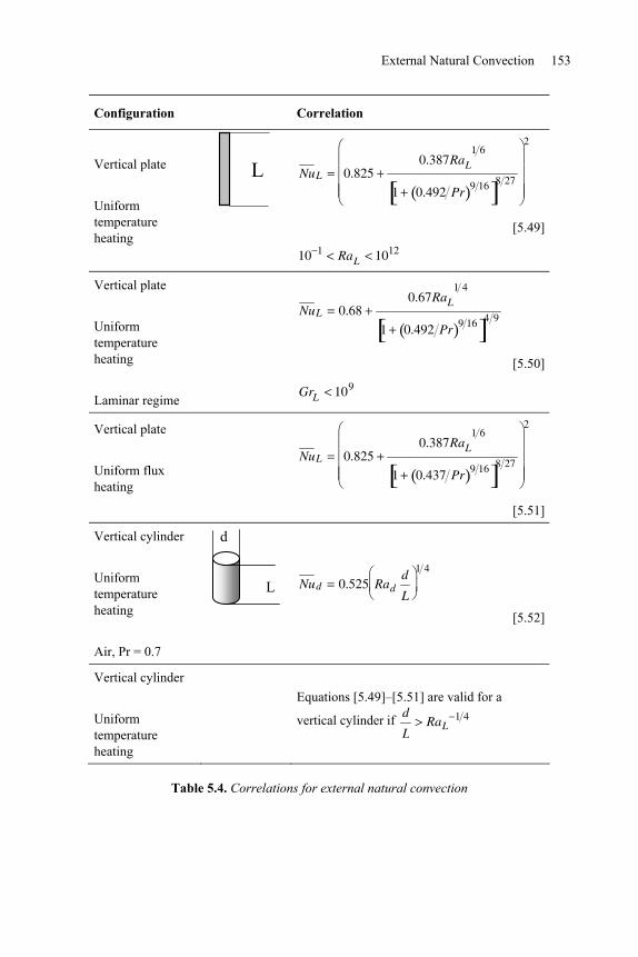
External Natural Convection 153
Configuration Correlation
Vertical plate Uniform temperature heating
L
NuL 0.8250.387RaL
1 6
1 0.492 Pr 9 16 8 27
2
[5.49]
10 1 RaL 1012
Vertical plate Uniform temperature heating Laminar regime
NuL 0.680.67RaL
1 4
1 0.492 Pr 9 16 4 9
[5.50]
GrL 109
Vertical plate Uniform flux heating
NuL 0.825
0.387RaL
1 6
1 0.437 Pr 9 16 8 27
2
[5.51]
Vertical cylinder Uniform temperature heating Air, Pr = 0.7
Nud 0.525 Rad
d
L
1 4
[5.52]
Vertical cylinder Uniform temperature heating
Equations [5.49]–[5.51] are valid for a
vertical cylinder if d
LRaL
1 4
Table 5.4. Correlations for external natural convection
L
d
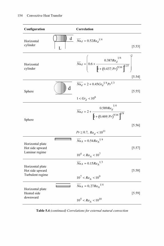
154 Convective Heat Transfer
Configuration Correlation
Horizontal cylinder
L
dNud 0.52Rad
1 4
[5.53]
Horizontal cylinder
Nud 0.60.387Rad
1 6
1 0.437 Pr 9 16 8 27
2
[5.54]
Sphere d
Nud 2 0.45Grd1 4Pr1 3
[5.55]
1 Grd 106
Sphere
Nud 20.589Rad
1 4
1 0.469 Pr 9 16 4 9
[5.56]
Pr 0.7, Rad 1011
Horizontal plate Hot side upward Laminar regime
NuA 0.54RaA1 4
[5.57]
104 RaA 107
Horizontal plate Hot side upward Turbulent regime
NuA 0.15RaA1 3
[5.58]
107 RaA 109
Horizontal plate Heated side downward
NuA 0, 27RaA1 4
[5.59]
105 RaA 1010
Table 5.4 (continued) Correlations for external natural convection
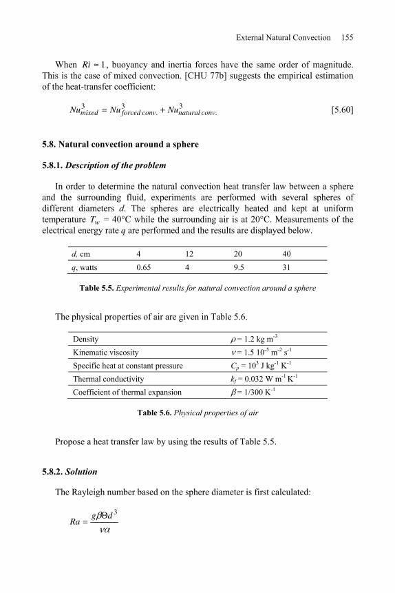
External Natural Convection 155
When Ri 1 , buoyancy and inertia forces have the same order of magnitude. This is the case of mixed convection. [CHU 77b] suggests the empirical estimation of the heat-transfer coefficient:
Numixed3 Nu forced conv.
3 Nunatural conv.3 [5.60]
5.8. Natural convection around a sphere
5.8.1. Description of the problem
In order to determine the natural convection heat transfer law between a sphere and the surrounding fluid, experiments are performed with several spheres of different diameters d. The spheres are electrically heated and kept at uniform temperature Tw = 40°C while the surrounding air is at 20°C. Measurements of the electrical energy rate q are performed and the results are displayed below.
d, cm 4 12 20 40 q, watts 0.65 4 9.5 31
Table 5.5. Experimental results for natural convection around a sphere
The physical properties of air are given in Table 5.6.
Density = 1.2 kg m-3 Kinematic viscosity = 1.5 10-5 m-2 s-1 Specific heat at constant pressure Cp = 103 J kg-1 K-1 Thermal conductivity kf = 0.032 W m-1 K-1 Coefficient of thermal expansion = 1/300 K-1
Table 5.6. Physical properties of air
Propose a heat transfer law by using the results of Table 5.5.
5.8.2. Solution
The Rayleigh number based on the sphere diameter is first calculated:
Rag d 3
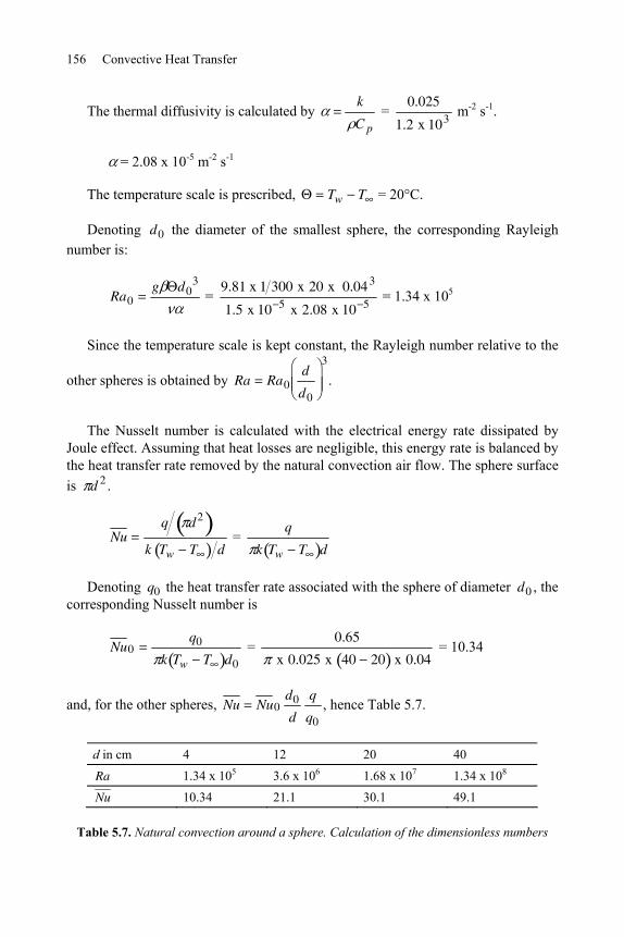
156 Convective Heat Transfer
The thermal diffusivity is calculated by k
C p
= 0.025
1.2 x 10³ m-2 s-1.
= 2.08 x 10⁻⁵ m-2 s-1
The temperature scale is prescribed, Tw T = 20°C.
Denoting d0 the diameter of the smallest sphere, the corresponding Rayleigh number is:
Ra0g d0
3 =
9.81 x 1 300 x 20 x 0.043
1.5 x 10 5 x 2.08 x 10 5 = 1.34 x 10⁵
Since the temperature scale is kept constant, the Rayleigh number relative to the
other spheres is obtained by Ra Ra0d
d0
3
.
The Nusselt number is calculated with the electrical energy rate dissipated by Joule effect. Assuming that heat losses are negligible, this energy rate is balanced by the heat transfer rate removed by the natural convection air flow. The sphere surface is d 2 .
Nuq d2
k Tw T d =
q
k Tw T d
Denoting q0 the heat transfer rate associated with the sphere of diameter d0 , the corresponding Nusselt number is
Nu0q0
k Tw T d0 =
0.65
x 0.025 x 40 20 x 0.04 = 10.34
and, for the other spheres, Nu Nu0d0
d
q
q0, hence Table 5.7.
d in cm 4 12 20 40
Ra 1.34 x 10⁵ 3.6 x 10⁶ 1.68 x 10⁷ 1.34 x 10⁸
Nu 10.34 21.1 30.1 49.1
Table 5.7. Natural convection around a sphere. Calculation of the dimensionless numbers
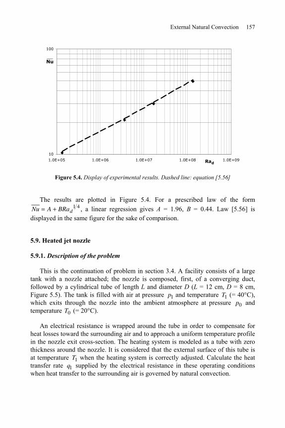
External Natural Convection 157
10
100
1.0E+05 1.0E+06 1.0E+07 1.0E+08 1.0E+09
Nu
Rad
Figure 5.4. Display of experimental results. Dashed line: equation [5.56]
The results are plotted in Figure 5.4. For a prescribed law of the form Nu A BRad
1 4 , a linear regression gives A = 1.96, B = 0.44. Law [5.56] is displayed in the same figure for the sake of comparison.
5.9. Heated jet nozzle
5.9.1. Description of the problem
This is the continuation of problem in section 3.4. A facility consists of a large tank with a nozzle attached; the nozzle is composed, first, of a converging duct, followed by a cylindrical tube of length L and diameter D (L = 12 cm, D = 8 cm, Figure 5.5). The tank is filled with air at pressure p1 and temperature T1 (= 40°C), which exits through the nozzle into the ambient atmosphere at pressure p0 and temperature T0 (= 20°C).
An electrical resistance is wrapped around the tube in order to compensate for heat losses toward the surrounding air and to approach a uniform temperature profile in the nozzle exit cross-section. The heating system is modeled as a tube with zero thickness around the nozzle. It is considered that the external surface of this tube is at temperature T1 when the heating system is correctly adjusted. Calculate the heat transfer rate q1 supplied by the electrical resistance in these operating conditions when heat transfer to the surrounding air is governed by natural convection.
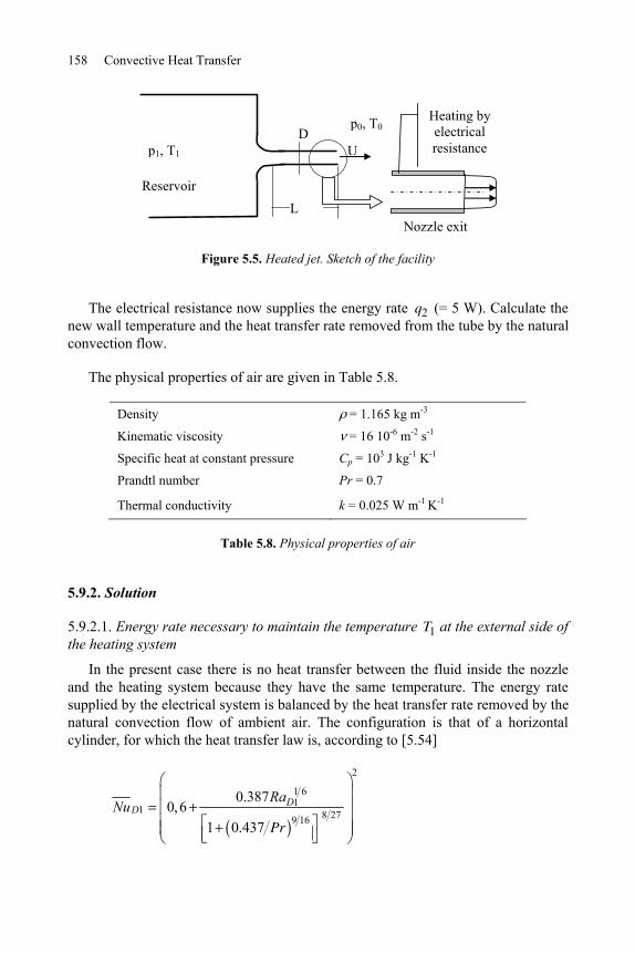
158 Convective Heat Transfer
p1, T1
p0, T0
L
D U
Nozzle exit
Reservoir
Heating by electrical resistance
Figure 5.5. Heated jet. Sketch of the facility
The electrical resistance now supplies the energy rate q2 (= 5 W). Calculate the new wall temperature and the heat transfer rate removed from the tube by the natural convection flow.
The physical properties of air are given in Table 5.8.
Density = 1.165 kg m-3
Kinematic viscosity = 16 10-6 m-2 s-1
Specific heat at constant pressure Cp = 103 J kg-1 K-1
Prandtl number Pr = 0.7
Thermal conductivity k = 0.025 W m-1 K-1
Table 5.8. Physical properties of air
5.9.2. Solution
5.9.2.1. Energy rate necessary to maintain the temperature T1 at the external side of the heating system
In the present case there is no heat transfer between the fluid inside the nozzle and the heating system because they have the same temperature. The energy rate supplied by the electrical system is balanced by the heat transfer rate removed by the natural convection flow of ambient air. The configuration is that of a horizontal cylinder, for which the heat transfer law is, according to [5.54]
2
1 61
1 8 279 16
0.3870,6
1 0.437
DD
RaNu
Pr
External Natural Convection 159
with RaD1g T1 T0 D3
= 9.81 x 1 303 x 40 20 x 0.083
16 x 10 6 x 16 x 10 6 0.7 = 9.06 x 10⁵.
The result is NuD1 = 14.5.
According to [5.48], the heat transfer rate exchanged with the ambient fluid is:
q1 Lk T1 T0 NuD1 = x 0.12 x 0.025 x 40 20 x 14.5 = 2.7 W.
It is also the electrical energy rate necessary to maintain the external side of the heating system at temperature T1.
It is worth noting that the problem in section 3.4 considered the start of heating and that the wall was at temperature T0 in these conditions. The heat transfer rate lost by the inner fluid was used to heat the nozzle tube and was higher than the heat transfer rate exchanged with the ambient fluid in the present problem. In the present case, the wall is at temperature T1 and the electrical energy rate is entirely lost toward the ambient fluid.
5.9.2.2. Overheating of the nozzle
When a higher electrical energy rate q2 q1 is supplied to the nozzle, the heating system becomes hotter than both the ambient fluid and the fluid inside the nozzle. It follows that the electrical energy rate q2 , dissipated by Joule effect, is used to heat both the ambient fluid (heat transfer rate qnat.conv. ) and the fluid inside the nozzle (heat transfer rate qforced.conv.).
q2 qnat.conv. q forced.conv. [5.61]
We assume that the heating system temperature is uniform. It is denoted T2 or in dimensionless form:
T2 T0
T1 T0 [5.62]
The new Rayleigh number may be expressed as a function of RaD1, which is already calculated in section 5.9.2.1
RaD2 RaD1
160 Convective Heat Transfer
and the corresponding Nusselt number is
NuD2 0.6 B 1 6 2
where 8 279 161 6
10.387 1 0.437DB Ra Pr .
The heat transfer rate exchanged by natural convection is finally:
qnat.conv. Lk T1 T0 NuD2
The heat transfer rate exchanged by forced convection is given (problem in section 3.4) by
qforced.conv. Dk T2 T1 NuL
with NuL 0.664 ReL Pr1 3 136.8 .
Accounting for the definition of , we have T2 T1 T1 T0 1 .
Thus, according to [5.61], the dimensionless temperature satisfies
q2 Lk T1 T0 NuD2 Dk T1 T0 NuL 1
or
AL
D0.6 B 1 6 2
NuL 1 [5.63]
where Aq2
Dk T1 T0.
With the numerical data of the problem, we find A = 39.8, B = 3.22 so that equation [5.63] becomes:
39.8 1.5 0.6 3.22 1 6 2136.8 1
External Natural Convection 161
As a first approximation, we consider 1 6 1 in this equation, which then becomes linear and gives = 1.113. Taking 1 6 into account, it is found that:
= 1.109.
The wall temperature is then T2 = 42.2°C.
The heat transfer rate supplied to the inner fluid is given by
qforced.conv. Dk T1 T0 NuL 1 = 2.17 W
and the heat transfer rate removed by the ambient fluid is
qnat.conv. = 2.83 W.
This result is close to q1 , because the new wall temperature is not very different from T1.
5.10. Shear stress on a vertical wall heated at uniform temperature
5.10.1. Description of the problem
A vertical wall is heated at uniform temperature Tw in a very large reservoir filled with a fluid of Prandtl number larger than 1. The fluid temperature far from the wall is T (Tw T ). The fluid is characterized by the density , the kinematic viscosity and the coefficient of thermal expansion assumed to be constant. Coordinates are x along the vertical axis and y in the direction normal to the wall. For Pr > 1, the velocity and temperature profiles have the shape shown in Figure 5.1. How is the Boussinesq equation in x direction at the wall (y = 0) simplified?
Express the viscous term in this equation by using the wall shear stress 0 and the thermal boundary layer thickness T . Estimate 0 as a function of the Rayleigh number and the parameters of the problem.
Also estimate 0 with Figure 5.6 that represents the similarity velocity profiles for two different values of the Prandtl number. Show that the two estimations of 0 are equivalent.
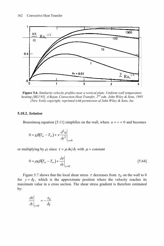
162 Convective Heat Transfer
ux
Rax-1/2
yx
Rax1/4
Figure 5.6. Similarity velocity profiles near a vertical plate. Uniform wall temperature heating [BEJ 95]. A Bejan, Convection Heat Transfer, 2nd edn, John Wiley & Sons, 1995
(New York) copyright, reprinted with permission of John Wiley & Sons, Inc
5.10.2. Solution
Boussinesq equation [5.11] simplifies on the wall, where u v 0 and becomes
0 g Tw T2u
y2y 0
or multiplying by , since u y with constant
0 g Tw Ty y 0
[5.64]
Figure 5.7 shows that the local shear stress decreases from 0 on the wall to 0 for y T , which is the approximate position where the velocity reaches its maximum value in a cross section. The shear stress gradient is therefore estimated by:
y y 0
0
T
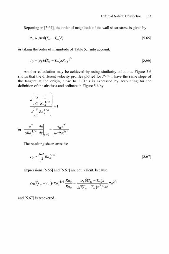
External Natural Convection 163
Reporting in [5.64], the order of magnitude of the wall shear stress is given by
0 g Tw T T [5.65]
or taking the order of magnitude of Table 5.1 into account,
0 g Tw T xRax1 4 [5.66]
Another calculation may be achieved by using similarity solutions. Figure 5.6 shows that the different velocity profiles plotted for Pr > 1 have the same slope of the tangent at the origin, close to 1. This is expressed by accounting for the definition of the abscissa and ordinate in Figure 5.6 by
dux 1
Rax1 / 2
dy
xRax
1 / 41
or x2
Rax3 / 4
du
dy y 0
= 0x2
Rax3 / 4
The resulting shear stress is:
0x2
Rax3 / 4 [5.67]
Expressions [5.66] and [5.67] are equivalent, because
g Tw T xRax1 4 Rax
Rax
g Tw T x
g Tw T x3Rax
3 4
and [5.67] is recovered.
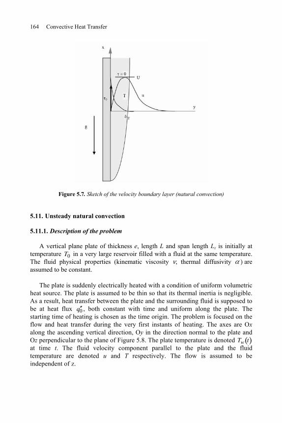
164 Convective Heat Transfer
Figure 5.7. Sketch of the velocity boundary layer (natural convection)
5.11. Unsteady natural convection
5.11.1. Description of the problem
A vertical plane plate of thickness e, length L and span length Lz is initially at temperature T0 in a very large reservoir filled with a fluid at the same temperature. The fluid physical properties (kinematic viscosity , thermal diffusivity are assumed to be constant.
The plate is suddenly electrically heated with a condition of uniform volumetric heat source. The plate is assumed to be thin so that its thermal inertia is negligible. As a result, heat transfer between the plate and the surrounding fluid is supposed to be at heat flux q 0 , both constant with time and uniform along the plate. The starting time of heating is chosen as the time origin. The problem is focused on the flow and heat transfer during the very first instants of heating. The axes are Ox along the ascending vertical direction, Oy in the direction normal to the plate and Oz perpendicular to the plane of Figure 5.8. The plate temperature is denoted Tw t at time t. The fluid velocity component parallel to the plate and the fluid temperature are denoted u and T respectively. The flow is assumed to be independent of z.
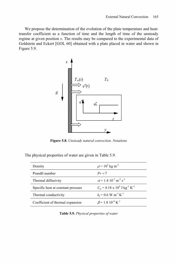
External Natural Convection 165
We propose the determination of the evolution of the plate temperature and heat-transfer coefficient as a function of time and the length of time of the unsteady regime at given position x. The results may be compared to the experimental data of Goldstein and Eckert [GOL 60] obtained with a plate placed in water and shown in Figure 5.9.
y
g
x
Tw(t) T0
q q 0
t
q t
Figure 5.8. Unsteady natural convection. Notations
The physical properties of water are given in Table 5.9.
Density = 103 kg m-3
Prandtl number Pr
Thermal diffusivity = 1.4 10-7 m-2 s-1
Specific heat at constant pressure Cp = 4.18 x 10³ J kg-1 K-1
Thermal conductivity kf = 0.6 W m-1 K-1
Coefficient of thermal expansion = 1.8 10-4 K-1
Table 5.9. Physical properties of water
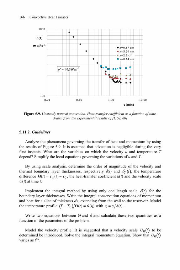
166 Convective Heat Transfer
100
1000
0.01 0.10 1.00 10.00
t (min)
h(t)
x=9.67 cmx=5.34 cmx=2.2 cmx=0.14 cm
W m2 K-1
q 49.3Wm 2
Figure 5.9. Unsteady natural convection. Heat-transfer coefficient as a function of time, drawn from the experimental results of [GOL 60]
5.11.2. Guidelines
Analyze the phenomena governing the transfer of heat and momentum by using the results of Figure 5.9. It is assumed that advection is negligible during the very first instants. What are the variables on which the velocity u and temperature T depend? Simplify the local equations governing the variations of u and T.
By using scale analysis, determine the order of magnitude of the velocity and thermal boundary layer thicknesses, respectively (t) and T t , the temperature difference (t) Tw (t) T0 , the heat-transfer coefficient h(t) and the velocity scale U(t) at time t.
Implement the integral method by using only one length scale t for the boundary layer thicknesses. Write the integral conservation equations of momentum and heat for a slice of thickness dx, extending from the wall to the reservoir. Model the temperature profile T T0 (t) ( ) with y (t)
Write two equations between and and calculate these two quantities as a function of the parameters of the problem.
Model the velocity profile. It is suggested that a velocity scale U0 t to be determined be introduced. Solve the integral momentum equation. Show that U0 t varies as t3/2.
External Natural Convection 167
Calculate the heat-transfer coefficient h(t). The exact solution to the thermal
problem gives h(t)2
k
t. Compare this expression to the result of the integral
method and to the experimental results in Figure 5.9.
Compare the experimental results that correspond to very long time in Figure 5.9, to those obtained from a heat transfer law in steady conditions.
Propose a method to determine the length of time td of the unsteady regime. Compare to the experimental results of Goldstein and Eckert [GOL 60]
5.11.3. Solution
5.11.3.1. Analysis of physical phenomena, equations and scale analysis
During the first instants of heating, heat is transferred by pure diffusion into water through a thin layer whose thickness only depends on time. The fluid is then set into motion by buoyancy forces and a boundary layer develops from the bottom edge of the plate. However, a fluid particle located at height x is initially unaware of the extremity effect coming from the plate bottom. This information arrives at the x-level with a time delay which depends on x. At given height, the transfer phenomena are purely diffusive and unsteady during the very first instants. Later on, advection comes into play and, finally, the steady regime is reached after a time delay which is increasing with x. Figure 5.9 shows that the heat-transfer coefficient h actually does not depend on x during the initial stage of heating, and then does not depend on t beyond a time length which is increasing with x.
In other words, the temperature and velocity fields do not depend on x during the initial stage of transfer. The velocity component u and the temperature T initially satisfy:
u x 0 , T x 0
The normal velocity component v is zero, according to the continuity equation. It follows that the advection terms are zero in the momentum and energy equations, which simplify in:
u
tg T T0
2u
y2 [5.68]
168 Convective Heat Transfer
T
t
2T
y2 [5.69]
It is worth noting that during this initial stage of transfer, the thermal and dynamic problems are uncoupled, contrary to the general case of natural convection. It is therefore possible to first solve the thermal problem, and, in a second step, the temperature field being calculated, to solve the dynamical problem.
It is also worth noting that the heat transfer problem is that of a stepwise variation of heat flux on a semi-infinite solid, whose solution is well known [ECK 72].
The above reasoning suggests representing the flow as shown in Figure 5.10.
Scale analysis gives the following orders of magnitude
T
t t,
2T
y2T
2
so that equation [5.69] gives the variation of T t with time
T t t [5.70]
T t is the depth of penetration by diffusion into a material of thermal diffusivity in unsteady conduction regime [ECK 72].
The heat flux is given by q 0 k T yy 0 , and estimated by q 0 k T ,
thus:
tq 0k
t [5.71]
The wall temperature increases as t1 2 .
The heat-transfer coefficient is defined by q 0 h , so that:
h tk
t [5.72]
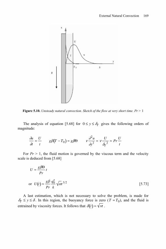
External Natural Convection 169
Figure 5.10. Unsteady natural convection. Sketch of the flow at very short time. Pr > 1
The analysis of equation [5.68] for 0 y T gives the following orders of magnitude:
u
t
U
t g T T0 g
2u
y2
U
T2
PrU
t
For Pr > 1, the fluid motion is governed by the viscous term and the velocity scale is deduced from [5.68]
Ug
Prt
or U tg
Pr
q 0k
t 3 2 [5.73]
A last estimation, which is not necessary to solve the problem, is made for T y . In this region, the buoyancy force is zero (T T0), and the fluid is
entrained by viscosity forces. It follows that t t .
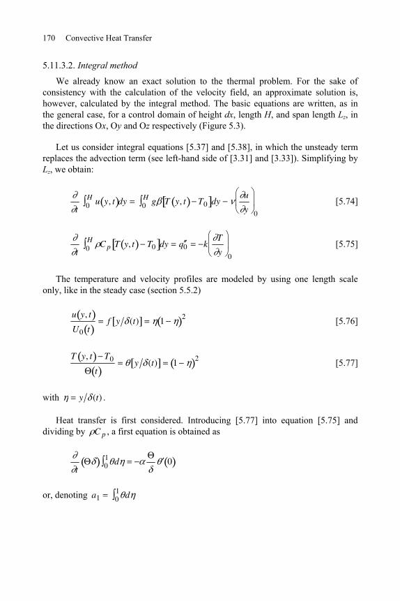
170 Convective Heat Transfer
5.11.3.2. Integral method
We already know an exact solution to the thermal problem. For the sake of consistency with the calculation of the velocity field, an approximate solution is, however, calculated by the integral method. The basic equations are written, as in the general case, for a control domain of height dx, length H, and span length Lz, in the directions Ox, Oy and Oz respectively (Figure 5.3).
Let us consider integral equations [5.37] and [5.38], in which the unsteady term replaces the advection term (see left-hand side of [3.31] and [3.33]). Simplifying by Lz, we obtain:
tu y, t0
H dy g0H T y, t T0 dy
u
y 0 [5.74]
t 0H C p T y, t T0 dy q 0 k
T
y 0
[5.75]
The temperature and velocity profiles are modeled by using one length scale only, like in the steady case (section 5.5.2)
u y, t
U0 tf y (t) 1 2
[5.76]
T y, t T0
ty (t) 1 2
[5.77]
with y (t) .
Heat transfer is first considered. Introducing [5.77] into equation [5.75] and dividing by C p , a first equation is obtained as
t 01 d 0
or, denoting a1 01 d
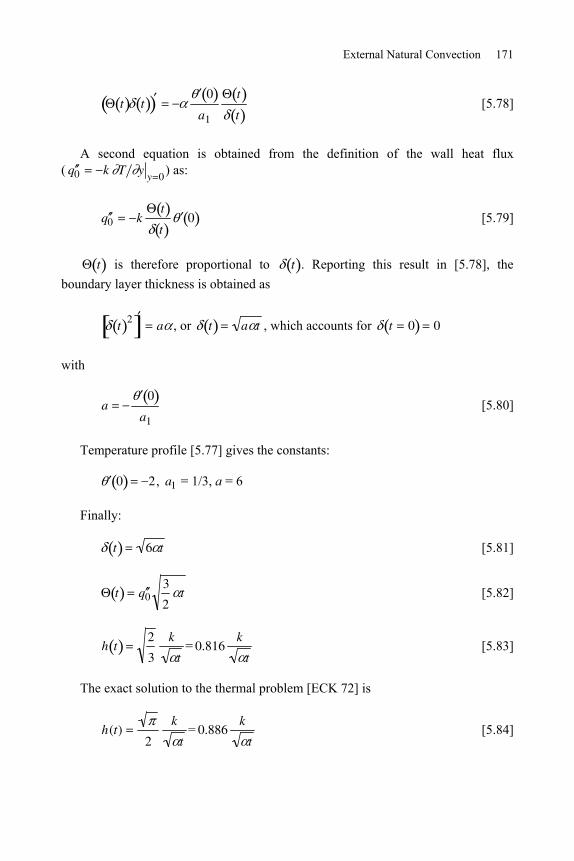
External Natural Convection 171
t t0
a1
t
t [5.78]
A second equation is obtained from the definition of the wall heat flux ( q 0 k T y
y 0) as:
q 0 kt
t0 [5.79]
t is therefore proportional to t . Reporting this result in [5.78], the boundary layer thickness is obtained as
t2
a , or t a t , which accounts for t 0 0
with
a0
a1 [5.80]
Temperature profile [5.77] gives the constants:
0 2 , a1 = 1/3, a = 6
Finally:
t 6 t [5.81]
t q 03
2t [5.82]
h t2
3
k
t= 0.816
k
t [5.83]
The exact solution to the thermal problem [ECK 72] is
h(t)2
k
t= 0.886
k
t [5.84]
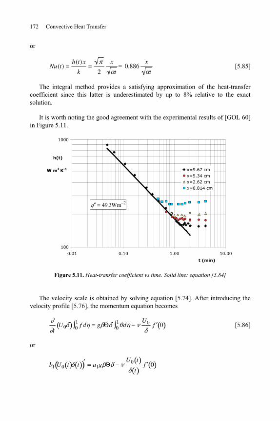
172 Convective Heat Transfer
or
Nu(t)h(t)x
k 2
x
t= 0.886
x
t [5.85]
The integral method provides a satisfying approximation of the heat-transfer coefficient since this latter is underestimated by up to 8% relative to the exact solution.
It is worth noting the good agreement with the experimental results of [GOL 60] in Figure 5.11.
100
1000
0.01 0.10 1.00 10.00
t (min)
h(t)
x=9.67 cmx=5.34 cmx=2.62 cmx=0.814 cm
W m2 K-1
q 49.3Wm 2
Figure 5.11. Heat-transfer coefficient vs time. Solid line: equation [5.84]
The velocity scale is obtained by solving equation [5.74]. After introducing the velocity profile [5.76], the momentum equation becomes
tU0 f0
1 d g 01 d
U0 f 0
[5.86]
or
b1 U0 t t a1gU0 t
tf 0
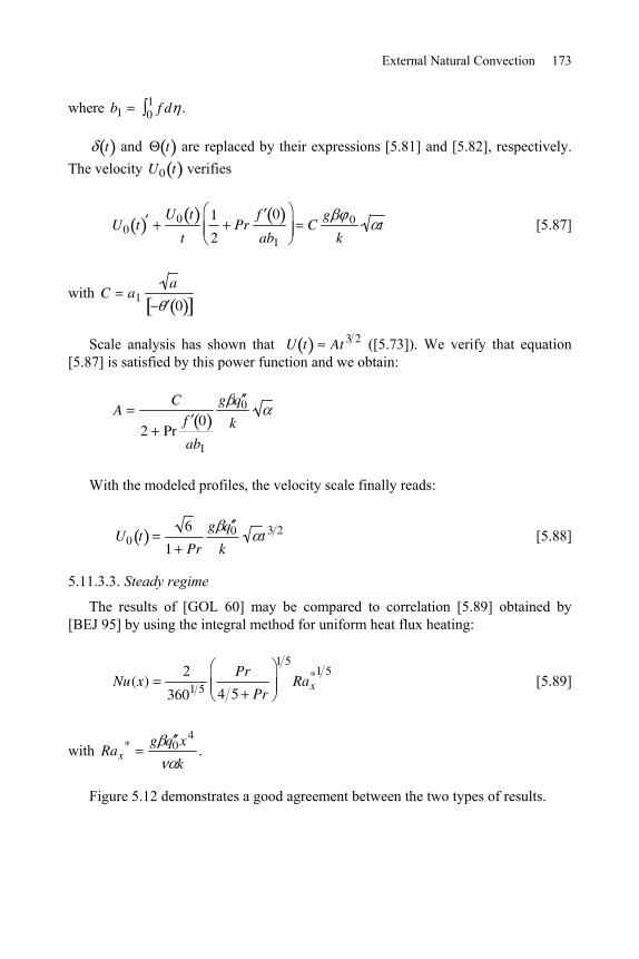
External Natural Convection 173
where b1 f01 d .
t and t are replaced by their expressions [5.81] and [5.82], respectively. The velocity U0 t verifies
U0 tU0 t
t
1
2Pr
f 0
ab1C
g 0
kt [5.87]
with C a1a
0
Scale analysis has shown that U t At 3 2 ([5.73]). We verify that equation [5.87] is satisfied by this power function and we obtain:
AC
2 Prf 0
ab1
g q 0k
With the modeled profiles, the velocity scale finally reads:
U0 t6
1 Pr
g q 0k
t 3 2 [5.88]
5.11.3.3. Steady regime
The results of [GOL 60] may be compared to correlation [5.89] obtained by [BEJ 95] by using the integral method for uniform heat flux heating:
Nu(x)2
3601 5
Pr
4 5 Pr
1 5
Rax*1 5
[5.89]
with Rax* g q 0x4
k.
Figure 5.12 demonstrates a good agreement between the two types of results.
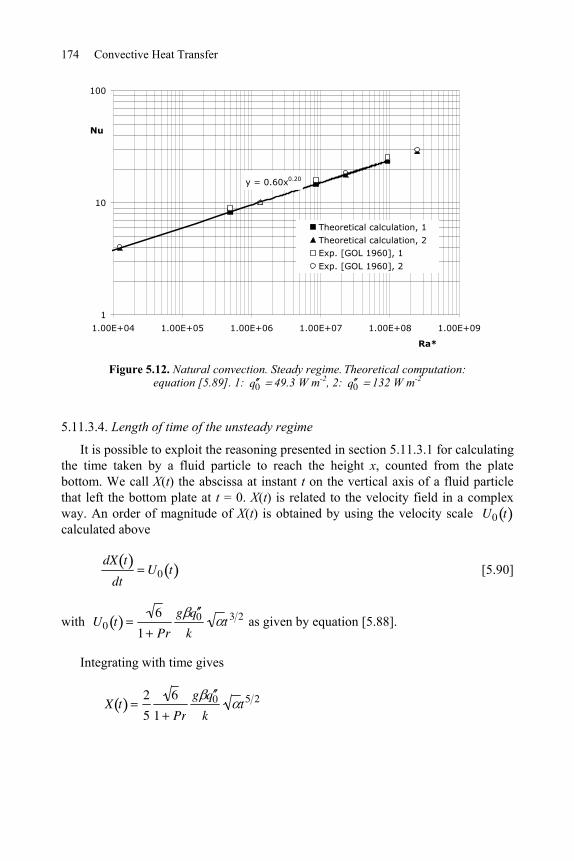
174 Convective Heat Transfer
y = 0.60x0.20
1
10
100
1.00E+04 1.00E+05 1.00E+06 1.00E+07 1.00E+08 1.00E+09
Ra*
Nu
Theoretical calculation, 1
Theoretical calculation, 2Exp. [GOL 1960], 1
Exp. [GOL 1960], 2
Figure 5.12. Natural convection. Steady regime. Theoretical computation: equation [5.89]. 1: q 0 49.3 W m-2, 2: q 0 132 W m-2
5.11.3.4. Length of time of the unsteady regime
It is possible to exploit the reasoning presented in section 5.11.3.1 for calculating the time taken by a fluid particle to reach the height x, counted from the plate bottom. We call X(t) the abscissa at instant t on the vertical axis of a fluid particle that left the bottom plate at t = 0. X(t) is related to the velocity field in a complex way. An order of magnitude of X(t) is obtained by using the velocity scale U0 t calculated above
dX t
dtU0 t [5.90]
with U0 t6
1 Pr
g q 0k
t 3 2 as given by equation [5.88].
Integrating with time gives
X t2
5
6
1 Pr
g q 0k
t5 2
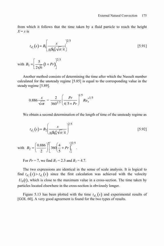
External Natural Convection 175
from which it follows that the time taken by a fluid particle to reach the height X = x is
td1x B1
x
g q 0 k
2 5
[5.91]
with B15
2 61 Pr
2 5
Another method consists of determining the time after which the Nusselt number calculated for the unsteady regime [5.85] is equal to the corresponding value in the steady regime [5.89].
0.886x
t =
2
3601 5
Pr
4 5 Pr
1 5
Rax*1 5
We obtain a second determination of the length of time of the unsteady regime as
td2x B2
x
g q 0 k
2 5
[5.92]
with B20.886
2
2
3604
5Pr
2 5
.
For Pr = 7, we find B1 = 2.3 and B2 = 4.7.
The two expressions are identical in the sense of scale analysis. It is logical to find td2
x td1x since the first calculation was achieved with the velocity
U0 t , which is close to the maximum value in a cross-section. The time taken by particles located elsewhere in the cross-section is obviously longer.
Figure 5.13 has been plotted with the time td2x and experimental results of
[GOL 60]. A very good agreement is found for the two types of results.
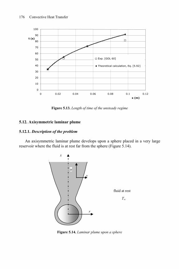
176 Convective Heat Transfer
Figure 5.13. Length of time of the unsteady regime
5.12. Axisymmetric laminar plume
5.12.1. Description of the problem
An axisymmetric laminar plume develops upon a sphere placed in a very large reservoir where the fluid is at rest far from the sphere (Figure 5.14).
x
r
u
v
fluid at rest
T
Figure 5.14. Laminar plume upon a sphere
0
10
20
30
40
50
60
70
80
90
100
0 0.02 0.04 0.06 0.08 0.1 0.12
x (m)
t (s)
Exp. [GOL 60]
Theoretical calculation, Eq. [5.92]
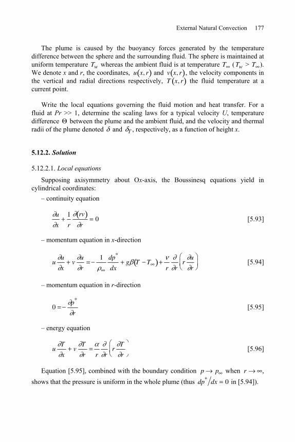
External Natural Convection 177
The plume is caused by the buoyancy forces generated by the temperature difference between the sphere and the surrounding fluid. The sphere is maintained at uniform temperature Tw whereas the ambient fluid is at temperature T (Tw > T ). We denote x and r, the coordinates, u x, r and v x, r , the velocity components in the vertical and radial directions respectively, T x, r the fluid temperature at a current point.
Write the local equations governing the fluid motion and heat transfer. For a fluid at Pr >> 1, determine the scaling laws for a typical velocity U, temperature difference between the plume and the ambient fluid, and the velocity and thermal radii of the plume denoted and T , respectively, as a function of height x.
5.12.2. Solution
5.12.2.1. Local equations
Supposing axisymmetry about Ox-axis, the Boussinesq equations yield in cylindrical coordinates:
– continuity equation
u
x
1
r
rv
r0 [5.93]
– momentum equation in x-direction
uu
xv
u
r
1 dp*
dxg T T
r rr
u
r [5.94]
– momentum equation in r-direction
0p*
r [5.95]
– energy equation
uT
xv
T
r r rr
T
r [5.96]
Equation [5.95], combined with the boundary condition p p when r , shows that the pressure is uniform in the whole plume (thus dp* dx 0 in [5.94]).
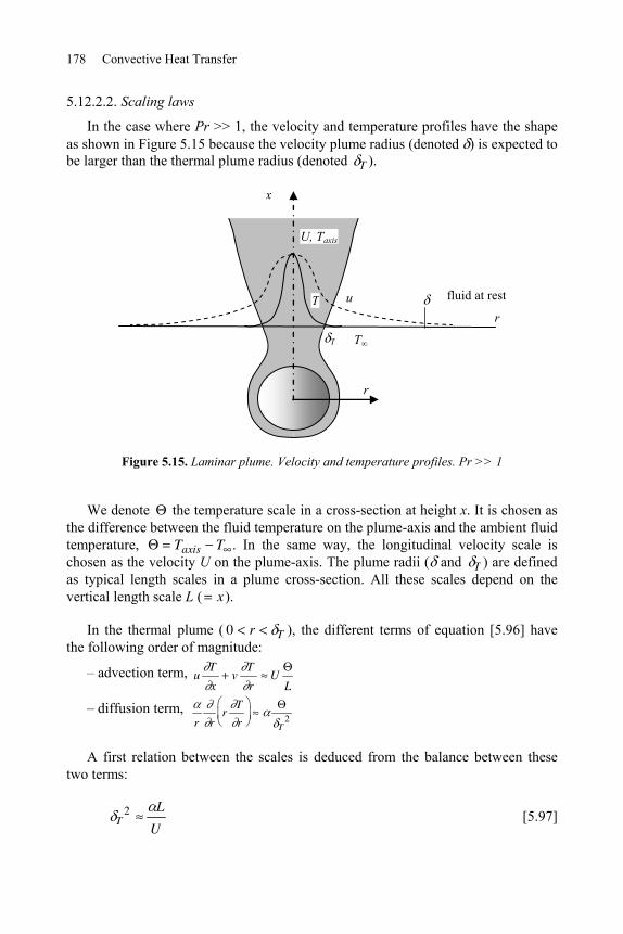
178 Convective Heat Transfer
5.12.2.2. Scaling laws
In the case where Pr >> 1, the velocity and temperature profiles have the shape as shown in Figure 5.15 because the velocity plume radius (denoted ) is expected to be larger than the thermal plume radius (denoted T ).
x
r
uT fluid at rest
TT
r
U, Taxis
Figure 5.15. Laminar plume. Velocity and temperature profiles. Pr >> 1
We denote the temperature scale in a cross-section at height x. It is chosen as the difference between the fluid temperature on the plume-axis and the ambient fluid temperature, Taxis T . In the same way, the longitudinal velocity scale is chosen as the velocity U on the plume-axis. The plume radii ( and T ) are defined as typical length scales in a plume cross-section. All these scales depend on the vertical length scale L ( x ).
In the thermal plume ( 0 r T ), the different terms of equation [5.96] have the following order of magnitude:
– advection term, uT
xv
T
rU
L
– diffusion term, r r
rT
r T2
A first relation between the scales is deduced from the balance between these two terms:
T2 L
U [5.97]
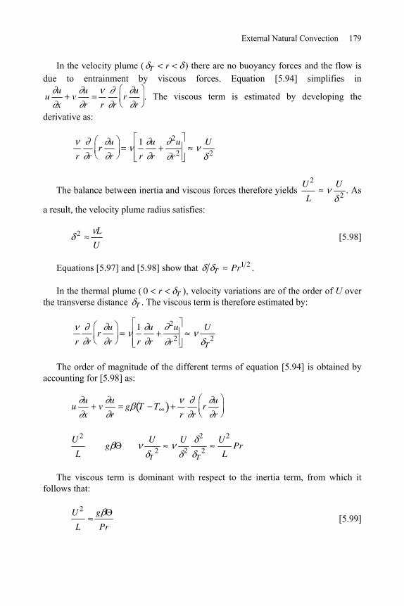
External Natural Convection 179
In the velocity plume ( T r ) there are no buoyancy forces and the flow is due to entrainment by viscous forces. Equation [5.94] simplifies in
uu
xv
u
r r rr
u
r. The viscous term is estimated by developing the
derivative as:
r rr
u
r
1
r
u
r
2u
r 2U
2
The balance between inertia and viscous forces therefore yields U 2
L
U2
. As
a result, the velocity plume radius satisfies:
2 L
U [5.98]
Equations [5.97] and [5.98] show that T Pr1 2 .
In the thermal plume ( 0 r T ), velocity variations are of the order of U over the transverse distance T . The viscous term is therefore estimated by:
r rr
u
r
1
r
u
r
2u
r2U
T2
The order of magnitude of the different terms of equation [5.94] is obtained by accounting for [5.98] as:
uu
xv
u
rg T T
r rr
u
r
U 2
L g
U
T2
U2
2
T2
U2
LPr
The viscous term is dominant with respect to the inertia term, from which it follows that:
U 2
L
g
Pr [5.99]
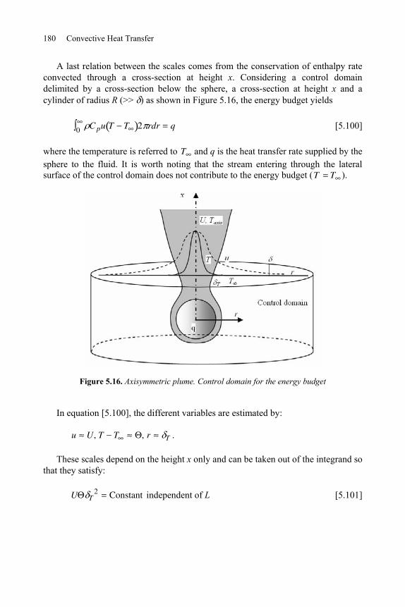
180 Convective Heat Transfer
A last relation between the scales comes from the conservation of enthalpy rate convected through a cross-section at height x. Considering a control domain delimited by a cross-section below the sphere, a cross-section at height x and a cylinder of radius R (>> ) as shown in Figure 5.16, the energy budget yields
C p0 u T T 2 rdr q [5.100]
where the temperature is referred to T and q is the heat transfer rate supplied by the sphere to the fluid. It is worth noting that the stream entering through the lateral surface of the control domain does not contribute to the energy budget (T T ).
Figure 5.16. Axisymmetric plume. Control domain for the energy budget
In equation [5.100], the different variables are estimated by:
u U, T T , r T .
These scales depend on the height x only and can be taken out of the integrand so that they satisfy:
U T2 Constant independent of L [5.101]
External Natural Convection 181
More precisely, there is a similarity solution for the velocity and thermal fields to the plume problem [GEB 71] so that
U T2 a
q
C p
[5.102]
where a is a numerical constant, which depends on the shape of the velocity and temperature profiles.
Combining [5.97] and [5.102], we determine the temperature scale on the plume axis:
cq
kL [5.103]
Combining [5.97], [5.99] and [5.102], the velocity scale is found to be:
U bg q
k
1 2 1
Pr1 2 [5.104]
The velocity scale U is independent of the vertical length scale, i.e. of the height of the cross-section considered for the computation.
Finally, the transverse length scale is:
T dk L2
g q
1 4
[5.105]
Relations [5.103] and [5.105] show that the temperature scale decreases as 1/x, whereas the plume radius increases as x .
Introducing the Rayleigh number
RaLg qL2
k [5.106]
equations [5.104] and [5.105] are expressed in the form
ULRaL
1 2 [5.107]
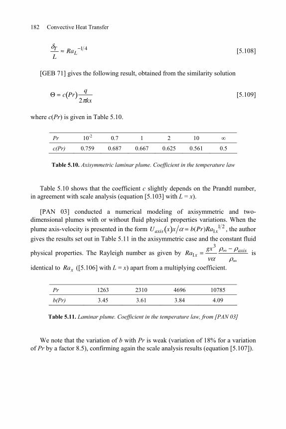
182 Convective Heat Transfer
T
LRaL
1 4 [5.108]
[GEB 71] gives the following result, obtained from the similarity solution
c Prq
2 kx [5.109]
where c(Pr) is given in Table 5.10.
Pr 10-2 0.7 1 2 10
c(Pr) 0.759 0.687 0.667 0.625 0.561 0.5
Table 5.10. Axisymmetric laminar plume. Coefficient in the temperature law
Table 5.10 shows that the coefficient c slightly depends on the Prandtl number, in agreement with scale analysis (equation [5.103] with L = x).
[PAN 03] conducted a numerical modeling of axisymmetric and two-dimensional plumes with or without fluid physical properties variations. When the plume axis-velocity is presented in the form Uaxis x x b(Pr)Ra1x
1 2 , the author gives the results set out in Table 5.11 in the axisymmetric case and the constant fluid
physical properties. The Rayleigh number as given by Ra1xgx3
axis is
identical to Rax ([5.106] with L = x) apart from a multiplying coefficient.
Pr 1263 2310 4696 10785
b(Pr) 3.45 3.61 3.84 4.09
Table 5.11. Laminar plume. Coefficient in the temperature law, from [PAN 03]
We note that the variation of b with Pr is weak (variation of 18% for a variation of Pr by a factor 8.5), confirming again the scale analysis results (equation [5.107]).
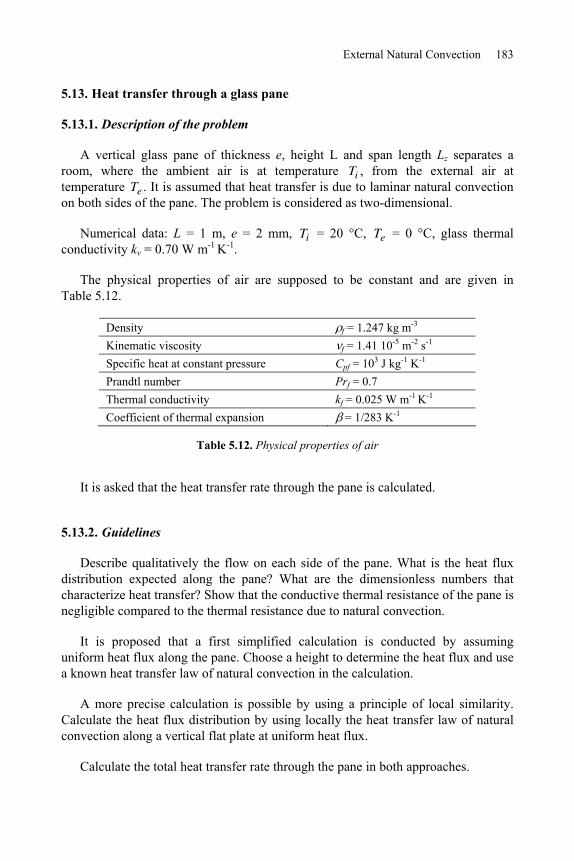
External Natural Convection 183
5.13. Heat transfer through a glass pane
5.13.1. Description of the problem
A vertical glass pane of thickness e, height L and span length Lz separates a room, where the ambient air is at temperature Ti , from the external air at temperature Te . It is assumed that heat transfer is due to laminar natural convection on both sides of the pane. The problem is considered as two-dimensional.
Numerical data: L = 1 m, e = 2 mm, Ti = 20 °C, Te = 0 °C, glass thermal conductivity kv = 0.70 W m-1 K-1.
The physical properties of air are supposed to be constant and are given in Table 5.12.
Density f = 1.247 kg m-3 Kinematic viscosity f = 1.41 10-5 m-2 s-1 Specific heat at constant pressure Cpf = 103 J kg-1 K-1 Prandtl number Prf = 0.7 Thermal conductivity kf = 0.025 W m-1 K-1 Coefficient of thermal expansion = 1/283 K-1
Table 5.12. Physical properties of air
It is asked that the heat transfer rate through the pane is calculated.
5.13.2. Guidelines
Describe qualitatively the flow on each side of the pane. What is the heat flux distribution expected along the pane? What are the dimensionless numbers that characterize heat transfer? Show that the conductive thermal resistance of the pane is negligible compared to the thermal resistance due to natural convection.
It is proposed that a first simplified calculation is conducted by assuming uniform heat flux along the pane. Choose a height to determine the heat flux and use a known heat transfer law of natural convection in the calculation.
A more precise calculation is possible by using a principle of local similarity. Calculate the heat flux distribution by using locally the heat transfer law of natural convection along a vertical flat plate at uniform heat flux.
Calculate the total heat transfer rate through the pane in both approaches.
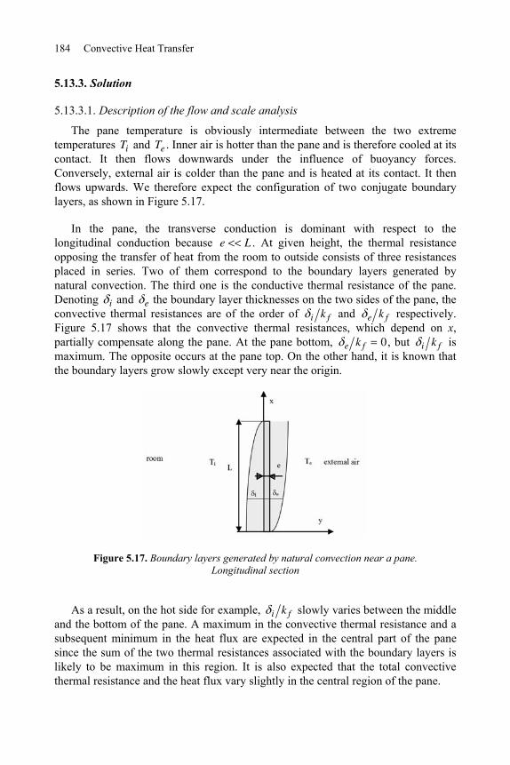
184 Convective Heat Transfer
5.13.3. Solution
5.13.3.1. Description of the flow and scale analysis
The pane temperature is obviously intermediate between the two extreme temperatures Ti and Te . Inner air is hotter than the pane and is therefore cooled at its contact. It then flows downwards under the influence of buoyancy forces. Conversely, external air is colder than the pane and is heated at its contact. It then flows upwards. We therefore expect the configuration of two conjugate boundary layers, as shown in Figure 5.17.
In the pane, the transverse conduction is dominant with respect to the longitudinal conduction because e L . At given height, the thermal resistance opposing the transfer of heat from the room to outside consists of three resistances placed in series. Two of them correspond to the boundary layers generated by natural convection. The third one is the conductive thermal resistance of the pane. Denoting i and e the boundary layer thicknesses on the two sides of the pane, the convective thermal resistances are of the order of i k f and e k f respectively. Figure 5.17 shows that the convective thermal resistances, which depend on x, partially compensate along the pane. At the pane bottom, e k f 0 , but i k f is maximum. The opposite occurs at the pane top. On the other hand, it is known that the boundary layers grow slowly except very near the origin.
Figure 5.17. Boundary layers generated by natural convection near a pane. Longitudinal section
As a result, on the hot side for example, i k f slowly varies between the middle and the bottom of the pane. A maximum in the convective thermal resistance and a subsequent minimum in the heat flux are expected in the central part of the pane since the sum of the two thermal resistances associated with the boundary layers is likely to be maximum in this region. It is also expected that the total convective thermal resistance and the heat flux vary slightly in the central region of the pane.
External Natural Convection 185
Scale analysis of section 5.3 (Table 5.1) shows that for Pr ~ 1, T L RaL-1/4 .
Otherwise, the conductive thermal resistance of the pane is e kv .
The ratio of the thermal resistances is therefore:
Thermal resistance by convection
Thermal resistance by conduction
kv
k f
L
e
1
RaL1 4
Denoting 0 Ti Te, we obtain with the data of the problem:
RaLg 0L3
= 2.44 109, Thermal resistance by convection
Thermal resistance by conduction63
This estimation demonstrates that the conductive thermal resistance may be ignored with respect to the convective thermal resistance. This is equivalent to ignoring temperature variations in a cross-section of the pane, in other words to consider a uniform pane temperature Tw x at given height x.
5.13.3.2. Global approach
In a first approach, we ignore the variations of heat flux along the pane and we use the heat transfer law [5.35] for natural convection along a vertical plane heated at uniform wall heat flux. Thus
Nu(x) b Pr Rax*1 5
with b(Pr)Pr
4 9Pr1 2 10Pr
1 5
,
Nu(x)q 0
k Tw(x) T x and Rax
* g q 0x4
k.
where q 0 denotes the heat flux. The reasoning of the previous paragraph suggests that we apply this relation with x = L/2, where the pane temperature is Ti Te 2 , for symmetry reasons.
Nu(x L 2)q 0
kTw(x L 2) T
L 2
with T Ti or T Te , according to
whether we consider the heat exchange with inner or external air. In both cases, Tw(x L 2) T 0 2 .
186 Convective Heat Transfer
Heat transfer is characterized by a global Nusselt number, built with 0 Ti Te and the total height of the pane L:
NuLq 0
k f 0 L [5.110]
With this definition, we find NuL Nu(x L 2) . The reason is that NuL has been defined with 0 and not with the temperature difference between the wall and the far fluid.
Denoting RaL 0
g 0L3, the Rayleigh number used in the previous
equations is given by Rax L 2* NuL
24RaL 0
.
Heat transfer law [5.35] becomes
NuL b PrNuL
24RaL 0
1 5
or
NuL
RaL 0
1 4
b Pr 5 4
2 [5.111]
For Pr = 0.72, equation [5.35] gives b(Pr) 0.519, from which it follows:
NuL
RaL 0
1 40.220
With the numerical data, RaL 0 = 2.44 109, NuL = 48.9.
q 0 k f 0 L NuL = 24.4 W m-2
q Lz q 0L= 24.4 W m-1
External Natural Convection 187
5.13.3.3. Local similarity approach
The heat transfer law [5.35] is used with the local heat flux q x , which is now a function of x. We write a relation between q x and the temperature difference Ti Tw x on the inner side on the one hand, and between q x and the temperature difference Tw x Te on the external side on the other hand. As a result, we obtain a system of two equations in the two unknowns q x , Tw x .
Denoting q 1 k f 0 L , x* x
L, x*
Tw x* Te
0 and q * x*
q x*
q 1,
the Nusselt and Rayleigh numbers are
* *
*
*x
x xNu
x,
0
* * *4*x LRa Ra x x
so that the heat transfer law, written on the external side becomes
q * x*x* 5 4
x*1 4b Pr 5 4 RaL 0
1 4 [5.112]
The heat transfer law on the inner side is obtained by substituting x* by 1 x* and by 1 in the above relation (note that it is the same heat flux on the internal and external sides of the pane, owing to continuity of heat flux through the pane):
0
5 4*
5 4" * 1 41 4*
1*
1L
xq x b Ra
xPr [5.113]
Combining the two equations, we obtain
x* 5 4
x*1 4
1 x*5 4
1 x* 1 4
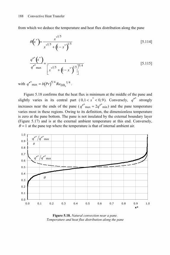
188 Convective Heat Transfer
from which we deduce the temperature and heat flux distribution along the pane
x* x*1 5
x*1 51 x* 1 5
[5.114]
q * x*
q *max
1
x*1 51 x* 1 5 5 4
[5.115]
with q *max b Pr 5 4 RaL 0
1 4 .
Figure 5.18 confirms that the heat flux is minimum at the middle of the pane and slightly varies in its central part ( 0,1 x* 0, 9 ). Conversely, q * strongly increases near the ends of the pane ( q *
max 2q *min) and the pane temperature
varies most in these regions. Owing to its definition, the dimensionless temperature is zero at the pane bottom. The pane is not insulated by the external boundary layer (Figure 5.17) and is at the external ambient temperature at this end. Conversely,
1 at the pane top where the temperature is that of internal ambient air.
0.0
0.1
0.2
0.3
0.4
0.5
0.6
0.7
0.8
0.9
1.0
0.0 0.1 0.2 0.3 0.4 0.5 0.6 0.7 0.8 0.9 1.0
x*
q * q *max
q * q *max
Figure 5.18. Natural convection near a pane. Temperature and heat flux distribution along the pane
External Natural Convection 189
The total heat transfer rate per transverse unit length is:
1" " " * *1
0 0
L
zq L q x dx q L q x dx
The integral is easily calculated by a numerical method, 1 " * *
0q x dx = 0.533.
Using the definition of NuL , the result is:
NuL
RaL 0
1 40.533b Pr 5 4 [5.116]
It is worth noting that the first approach gave a very similar result ([5.111]) (coefficient 0.5 instead of 0.533).
For Pr = 0,72, the heat transfer law is NuL
RaL 0
1 4 = 0.235.
When the same calculation as in the first approach is conducted, the previous result gives the heat transfer rate par transverse length:
q Lz = 26 W m-1
5.14. Mixed convection near a vertical wall with suction
5.14.1. Description of the problem
We consider mixed convection near a vertical plate, as shown in Figure 5.19. The flow results from a combination of natural and forced convection. The wall is porous and is crossed by a uniform suction velocity flow (velocity v0 , counted positively for a suction). Suction prevents the thermal and velocity boundary layers from growing and, as a consequence, they are spatially uniform d dx d T dx 0 . Determine:
– the temperature and velocity distribution; – the friction coefficient C f w v0
2 . Separate the contributions of natural and forced convection to C f . Discuss.
This problem is inspired by [ARP 84].
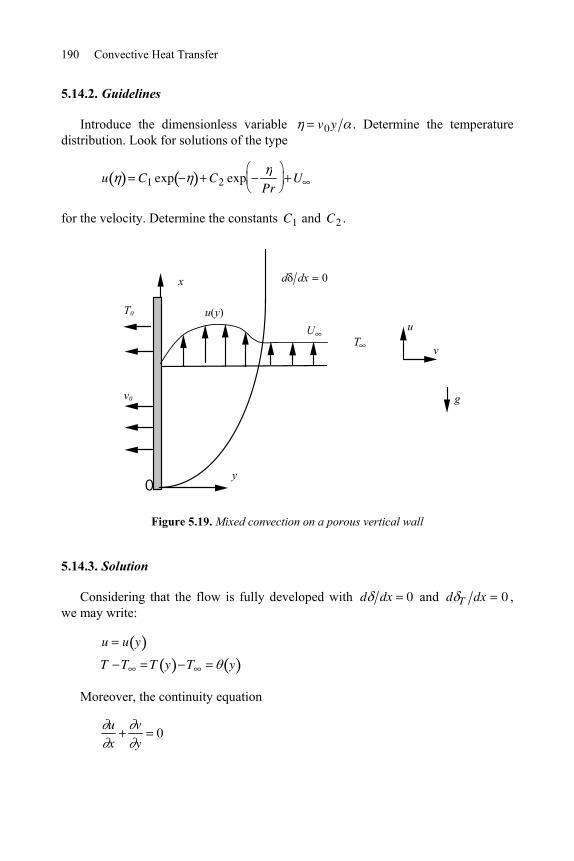
190 Convective Heat Transfer
5.14.2. Guidelines
Introduce the dimensionless variable v0y . Determine the temperature distribution. Look for solutions of the type
u C1 exp C2 expPr
U
for the velocity. Determine the constants C1 and C2 .
0
T0
v0
y
x d dx 0
TU
v
u
g
u(y)
Figure 5.19. Mixed convection on a porous vertical wall
5.14.3. Solution
Considering that the flow is fully developed with d dx 0 and d T dx 0 , we may write:
u u y
T T T y T y
Moreover, the continuity equation
u
x
v
y0
External Natural Convection 191
implies
dv dy 0 and consequently v Constant v0
The momentum and energy equations become:
uu
xv
u
yv0
du
dy
d 2u
dy2g T T
uT
xv
T
yv0
dT
dy
d 2T
dy2
[5.117]
As a result, the temperature and velocity fields are uncoupled. System [5.117] is subjected to the following boundary conditions:
u 0 0, u U
T 0 T0, T T [5.118]
Denoting 0 T0 T , the energy equation is easily integrated as:
y T y T 0 expv0y
[5.119]
This equation shows that the dimensionless variable v0y is relevant for the temperature distribution 0 exp , which is completely governed by suction at the wall. The momentum equation takes the form of a non-linear inhomogeneous differential equation:
d 2u
dy2v0
du
dyg T T0 exp
v0y [5.120]
The velocity distribution u y is the sum of the solution to the homogeneous part of this equation and a particular solution. Following the guidelines given in section 5.14.2, u y is of the form:
u C1 exp C2 expPr
U
192 Convective Heat Transfer
The coefficients C1 and C2 are determined from the boundary conditions [5.118]. We obtain:
u
U
g 0
v02 1 Pr U
e e Pr 1 e Pr [5.121]
The limit of expression [5.121] for Pr 1 ( ) is:
u
U
g 0
v02U
e 1 e [5.122]
This is a problem of mixed convection, i.e. a combination of natural and forced convection. We expect therefore to recover the classical dimensionless numbers which govern the mechanisms involved in these phenomena, in other words the Grashof number and the Reynolds number respectively. Let us recall that the first one is given by:
Grg 0
2L3
The length scale L is clearly imposed in the present problem by the characteristic thermal scale Lt v0 , which appears in . The dimensionless group that appears in equation [5.121] may be written in the form
g 0
v02 1 Pr U
g 02 v0
3
Uv0
Pr
1 Pr
which obviously may be transformed as
g 0
v02 1 Pr U
GrLt
ReLt
Pr
1 Pr (Pr 1)
For Pr 1, the characteristic thermal scale also becomes the viscous length L v0 Lt . The dimensionless group in equation [5.122] may in turn be written in the form:
g 0
v02U
g 02 v0
3
Uv0
g 02 v0
3
Uv0
GrLt
ReLt
External Natural Convection 193
In sum, the velocity distribution is expressed as:
u
U
GrLt
ReLt
Pr
1 Pr e e Pr 1 e Pr Pr 1
u
U
GrLt
ReLte 1 e Pr 1
[5.123]
These relations are easily interpreted. The first groups of terms in the right-hand side represent the contribution of natural convection to the velocity field. This contribution is canceled when GrLt 0 and/or ReLt .
It is worth noting that the dimensionless number governing this problem of mixed convection is Gr Re and not Gr Re2 , as in the general case (section 5.7). This comes from the fact that the inertia term is proportional to U and not to U2 (equation [5.120]).
The friction coefficient is
C fw
v02
u y 0
v02
g 0
v03Pr
U
v0
and may be rearranged as
C f GrLtPr2 ReLtPr [5.124]

This page intentionally left blank
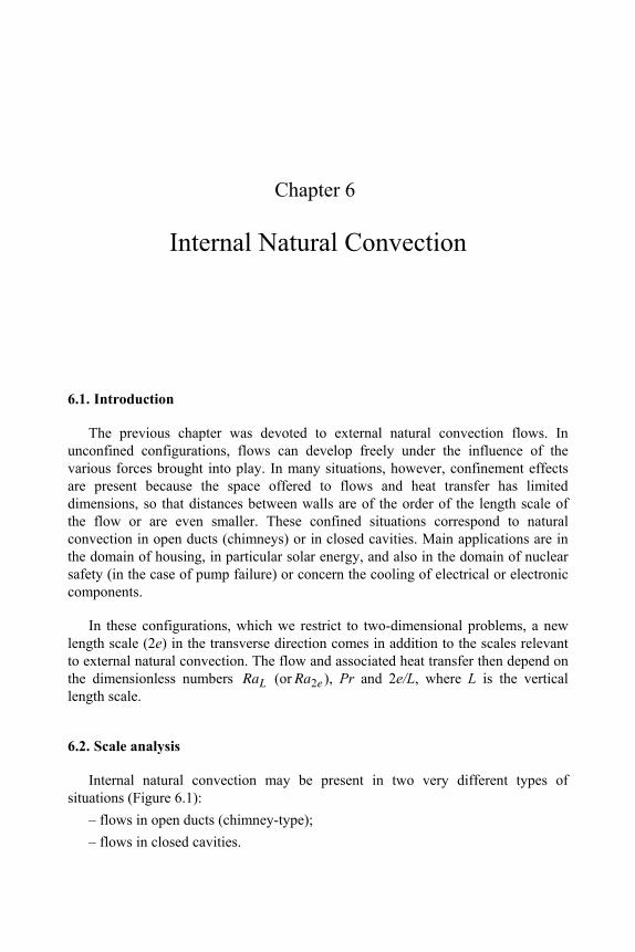
Chapter 6
Internal Natural Convection
6.1. Introduction
The previous chapter was devoted to external natural convection flows. In unconfined configurations, flows can develop freely under the influence of the various forces brought into play. In many situations, however, confinement effects are present because the space offered to flows and heat transfer has limited dimensions, so that distances between walls are of the order of the length scale of the flow or are even smaller. These confined situations correspond to natural convection in open ducts (chimneys) or in closed cavities. Main applications are in the domain of housing, in particular solar energy, and also in the domain of nuclear safety (in the case of pump failure) or concern the cooling of electrical or electronic components.
In these configurations, which we restrict to two-dimensional problems, a new length scale (2e) in the transverse direction comes in addition to the scales relevant to external natural convection. The flow and associated heat transfer then depend on the dimensionless numbers RaL (or Ra2e ), Pr and 2e/L, where L is the vertical length scale.
6.2. Scale analysis
Internal natural convection may be present in two very different types of situations (Figure 6.1):
– flows in open ducts (chimney-type); – flows in closed cavities.
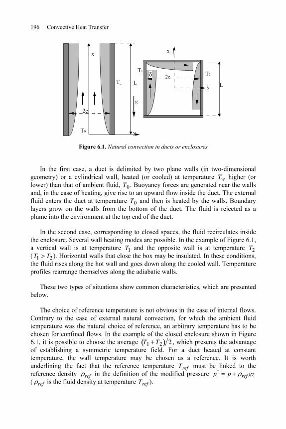
196 Convective Heat Transfer
2eL
x
y
g
2e
x
y
Tw
T0
L
T1 T2
Figure 6.1. Natural convection in ducts or enclosures
In the first case, a duct is delimited by two plane walls (in two-dimensional geometry) or a cylindrical wall, heated (or cooled) at temperature Tw higher (or lower) than that of ambient fluid, T0 . Buoyancy forces are generated near the walls and, in the case of heating, give rise to an upward flow inside the duct. The external fluid enters the duct at temperature T0 and then is heated by the walls. Boundary layers grow on the walls from the bottom of the duct. The fluid is rejected as a plume into the environment at the top end of the duct.
In the second case, corresponding to closed spaces, the fluid recirculates inside the enclosure. Several wall heating modes are possible. In the example of Figure 6.1, a vertical wall is at temperature T1 and the opposite wall is at temperature T2 (T1 T2 ). Horizontal walls that close the box may be insulated. In these conditions, the fluid rises along the hot wall and goes down along the cooled wall. Temperature profiles rearrange themselves along the adiabatic walls.
These two types of situations show common characteristics, which are presented below.
The choice of reference temperature is not obvious in the case of internal flows. Contrary to the case of external natural convection, for which the ambient fluid temperature was the natural choice of reference, an arbitrary temperature has to be chosen for confined flows. In the example of the closed enclosure shown in Figure 6.1, it is possible to choose the average T1 T2 2 , which presents the advantage of establishing a symmetric temperature field. For a duct heated at constant temperature, the wall temperature may be chosen as a reference. It is worth underlining the fact that the reference temperature Tref must be linked to the reference density ref in the definition of the modified pressure p* p ref gz ( ref is the fluid density at temperature Tref ).
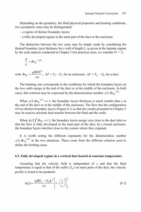
Internal Natural Convection 197
Depending on the geometry, the fluid physical properties and heating conditions, two asymptotic cases may be distinguished:
– a regime of distinct boundary layers; – a fully developed regime in the main part of the duct or the enclosure.
The distinction between the two cases may be simply made by considering the thermal boundary layer thickness for a wall of length L, as given in the laminar regime by the scale analysis conducted in Chapter 5 (for practical cases, we consider Pr > 1)
LRaL
1 4
with RaLg TL3
, T T1 T2 for an enclosure, T Tw T0 for a duct.
The limiting case corresponds to the conditions for which the boundary layers on the two walls merge at the end of the duct or at the middle of the enclosure. In both cases, this criterion may be expressed by the dimensionless number e L RaL
1 4 .
When e L RaL1 4 1, the boundary layers thickness is much smaller than e at
the end of the duct or at the middle of the enclosure. The flow has the configuration of two distinct boundary layers (Figure 6.1) so that the results presented in Chapter 5 may be used to calculate heat transfer between the fluid and the walls.
When e L4
RaL 1, the boundary layers merge very close to the duct inlet so that the flow is fully developed in the main part of the duct. In a closed enclosure, the boundary layers interfere close to the corners where they originate.
It is worth noting the different exponents for the dimensionless number e L RaL
1 4 in the two situations. These come from the different criterion used to define the limiting cases.
6.3. Fully developed regime in a vertical duct heated at constant temperature
Assuming that the velocity field is independent of x and that the fluid temperature is equal to that of the walls (Tw ) on most parts of the duct, the velocity profile is found to be parabolic
u yg Tw T0 e2
21
y
e
2
[6.1]
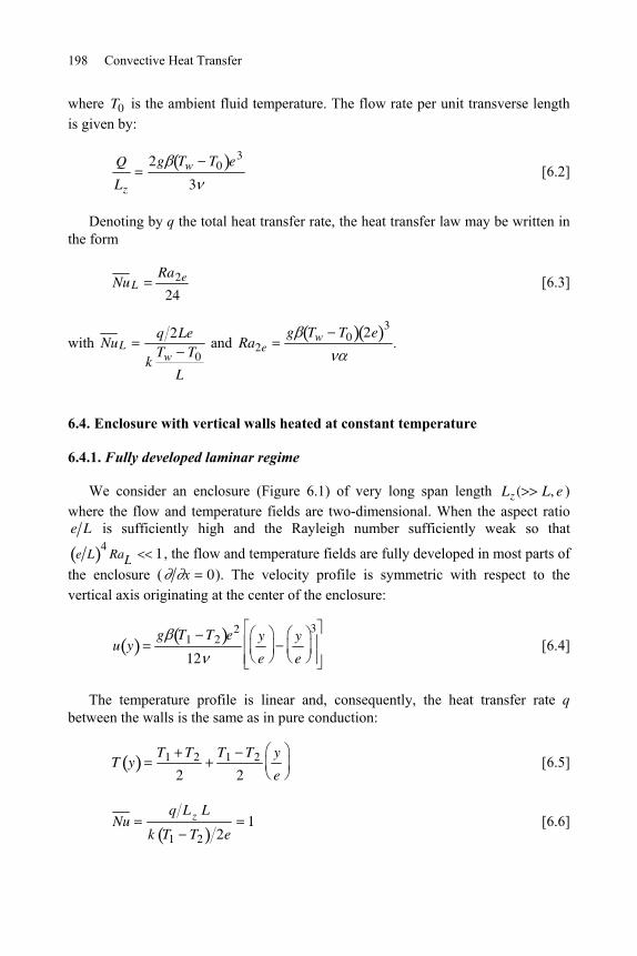
198 Convective Heat Transfer
where T0 is the ambient fluid temperature. The flow rate per unit transverse length is given by:
Q
Lz
2g Tw T0 e3
3
[6.2]
Denoting by q the total heat transfer rate, the heat transfer law may be written in the form
NuLRa2e
24 [6.3]
with NuLq 2Le
kTw T0
L
and Ra2eg Tw T0 2e 3
.
6.4. Enclosure with vertical walls heated at constant temperature
6.4.1. Fully developed laminar regime
We consider an enclosure (Figure 6.1) of very long span length Lz ( L, e ) where the flow and temperature fields are two-dimensional. When the aspect ratio e L is sufficiently high and the Rayleigh number sufficiently weak so that
e L4
RaL 1 , the flow and temperature fields are fully developed in most parts of the enclosure ( x 0). The velocity profile is symmetric with respect to the vertical axis originating at the center of the enclosure:
u yg T1 T2 e2
12
y
e
y
e
3
[6.4]
The temperature profile is linear and, consequently, the heat transfer rate q between the walls is the same as in pure conduction:
T yT1 T2
2
T1 T2
2
y
e
[6.5]
Nuq Lz L
k T1 T2 2e1
[6.6]
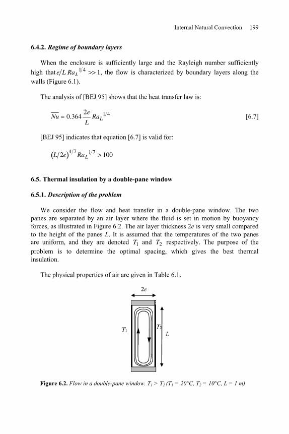
Internal Natural Convection 199
6.4.2. Regime of boundary layers
When the enclosure is sufficiently large and the Rayleigh number sufficiently high that e L RaL
1 4 1, the flow is characterized by boundary layers along the walls (Figure 6.1).
The analysis of [BEJ 95] shows that the heat transfer law is:
Nu 0.3642e
LRaL
1 4
[6.7]
[BEJ 95] indicates that equation [6.7] is valid for:
L 2e4 7
RaL1 7 100
6.5. Thermal insulation by a double-pane window
6.5.1. Description of the problem
We consider the flow and heat transfer in a double-pane window. The two panes are separated by an air layer where the fluid is set in motion by buoyancy forces, as illustrated in Figure 6.2. The air layer thickness 2e is very small compared to the height of the panes L. It is assumed that the temperatures of the two panes are uniform, and they are denoted T1 and T2 respectively. The purpose of the problem is to determine the optimal spacing, which gives the best thermal insulation.
The physical properties of air are given in Table 6.1.
Figure 6.2. Flow in a double-pane window. T1 > T2 (T1 = 20°C, T2 = 10°C, L = 1 m)
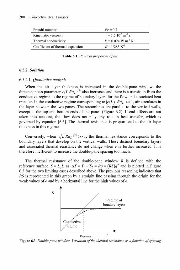
200 Convective Heat Transfer
Prandtl number PrKinematic viscosity = 1.5 10-5 m-2 s-1 Thermal conductivity kf = 0.024 W m-1 K-1 Coefficient of thermal expansion = 1/283 K-1
Table 6.1. Physical properties of air
6.5.2. Solution
6.5.2.1. Qualitative analysis
When the air layer thickness is increased in the double-pane window, the dimensionless parameter e L RaL
1 4 also increases and there is a transition from the conductive regime to the regime of boundary layers for the flow and associated heat transfer. In the conductive regime corresponding to e L
4RaL 1, air circulates in
the layer between the two panes. The streamlines are parallel to the vertical walls, except at the top and bottom ends of the panes (Figure 6.2). If end effects are not taken into account, the flow does not play any role in heat transfer, which is governed by equation [6.6]. The thermal resistance is proportional to the air layer thickness in this regime.
Conversely, when e L RaL1 4 1, the thermal resistance corresponds to the
boundary layers that develop on the vertical walls. These distinct boundary layers and associated thermal resistance do not change when e is further increased. It is therefore inefficient to increase the double-pane spacing too much.
The thermal resistance of the double-pane window R is defined with the reference surface S LzL as T T1 T2 Rq RS q and is plotted in Figure 6.3 for the two limiting cases described above. The previous reasoning indicates that RS is represented in this graph by a straight line passing through the origin for the weak values of e and by a horizontal line for the high values of e.
Figure 6.3. Double-pane window. Variation of the thermal resistance as a function of spacing
S
eoptimum
Conductive regime
e
Regime of boudary layers
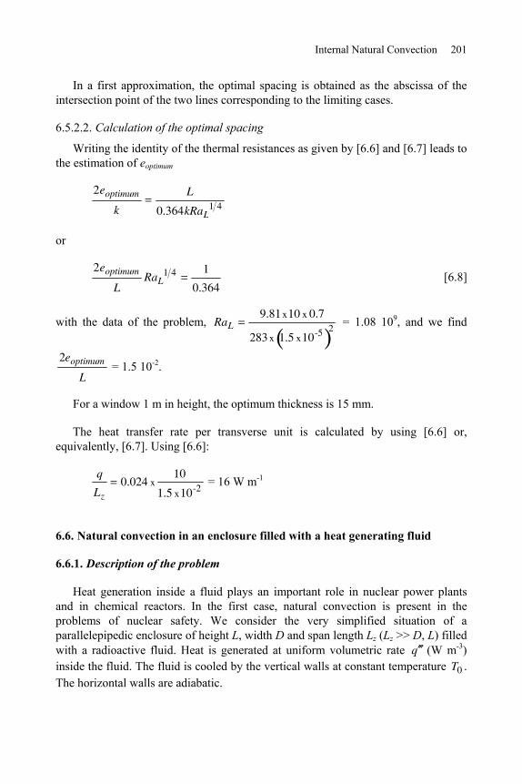
Internal Natural Convection 201
In a first approximation, the optimal spacing is obtained as the abscissa of the intersection point of the two lines corresponding to the limiting cases.
6.5.2.2. Calculation of the optimal spacing
Writing the identity of the thermal resistances as given by [6.6] and [6.7] leads to the estimation of eoptimum
2eoptimum
k
L
0.364kRaL1 4
or
2eoptimum
LRaL
1 4 1
0.364
[6.8]
with the data of the problem, RaL9.81x10 x 0.7
283 x 1.5 x10-5 2 = 1.08 109, and we find
2eoptimum
L = 1.5 10-2.
For a window 1 m in height, the optimum thickness is 15 mm.
The heat transfer rate per transverse unit is calculated by using [6.6] or, equivalently, [6.7]. Using [6.6]:
q
Lz
0.024 x10
1.5 x10-2 = 16 W m-1
6.6. Natural convection in an enclosure filled with a heat generating fluid
6.6.1. Description of the problem
Heat generation inside a fluid plays an important role in nuclear power plants and in chemical reactors. In the first case, natural convection is present in the problems of nuclear safety. We consider the very simplified situation of a parallelepipedic enclosure of height L, width D and span length Lz (Lz >> D, L) filled with a radioactive fluid. Heat is generated at uniform volumetric rate q (W m-3) inside the fluid. The fluid is cooled by the vertical walls at constant temperature T0 . The horizontal walls are adiabatic.
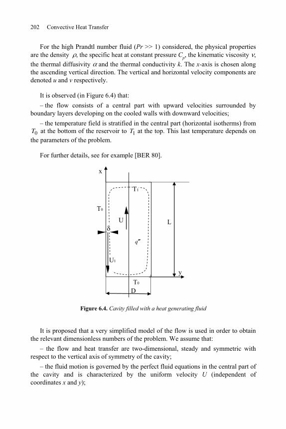
202 Convective Heat Transfer
For the high Prandtl number fluid (Pr >> 1) considered, the physical properties are the density , the specific heat at constant pressure Cp, the kinematic viscosity , the thermal diffusivity and the thermal conductivity k. The x-axis is chosen along the ascending vertical direction. The vertical and horizontal velocity components are denoted u and v respectively.
It is observed (in Figure 6.4) that: – the flow consists of a central part with upward velocities surrounded by
boundary layers developing on the cooled walls with downward velocities; – the temperature field is stratified in the central part (horizontal isotherms) from
T0 at the bottom of the reservoir to T1 at the top. This last temperature depends on the parameters of the problem.
For further details, see for example [BER 80].
U
T0
y
x
q
L
D
T1
T0
U1
Figure 6.4. Cavity filled with a heat generating fluid
It is proposed that a very simplified model of the flow is used in order to obtain the relevant dimensionless numbers of the problem. We assume that:
– the flow and heat transfer are two-dimensional, steady and symmetric with respect to the vertical axis of symmetry of the cavity;
– the fluid motion is governed by the perfect fluid equations in the central part of the cavity and is characterized by the uniform velocity U (independent of coordinates x and y);
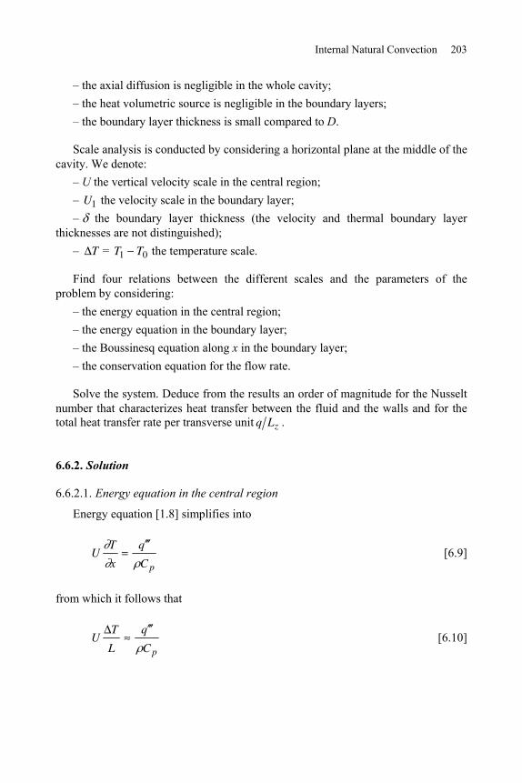
Internal Natural Convection 203
– the axial diffusion is negligible in the whole cavity; – the heat volumetric source is negligible in the boundary layers; – the boundary layer thickness is small compared to D.
Scale analysis is conducted by considering a horizontal plane at the middle of the cavity. We denote:
– U the vertical velocity scale in the central region; – U1 the velocity scale in the boundary layer; – the boundary layer thickness (the velocity and thermal boundary layer
thicknesses are not distinguished); – T = T1 T0 the temperature scale.
Find four relations between the different scales and the parameters of the problem by considering:
– the energy equation in the central region; – the energy equation in the boundary layer; – the Boussinesq equation along x in the boundary layer; – the conservation equation for the flow rate.
Solve the system. Deduce from the results an order of magnitude for the Nusselt number that characterizes heat transfer between the fluid and the walls and for the total heat transfer rate per transverse unit q Lz .
6.6.2. Solution
6.6.2.1. Energy equation in the central region
Energy equation [1.8] simplifies into
UT
x
q
C p
[6.9]
from which it follows that
UT
L
q
C p
[6.10]
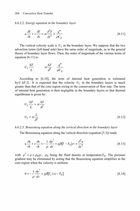
204 Convective Heat Transfer
6.6.2.2. Energy equation in the boundary layer
uT
xv
T
y
2T
y2
q
C p
[6.11]
The vertical velocity scale is U1 in the boundary layer. We suppose that the two advection terms (left-hand side) have the same order of magnitude, as in the general theory of boundary layer flows. Then, the order of magnitude of the various terms of equation [6.11] is:
U1T
L
T2
q
C p
According to [6.10], the term of internal heat generation is estimated byU T L . It is expected that the velocity U1 in the boundary layers is much greater than that of the core region owing to the conservation of flow rate. The term of internal heat generation is then negligible in the boundary layers so that thermal equilibrium is given by:
U1T
L
T2
U1L2
[6.12]
6.6.2.3. Boussinesq equation along the vertical direction in the boundary layer
The Boussinesq equation along the vertical direction (equation [5.3]) reads
uu
xv
u
y
1 dp*
dxg T T0
2u
y2 [6.13]
with p* p 0gx , 0 being the fluid density at temperatureT0 . The pressure gradient may be eliminated by noting that the Boussinesq equation simplifies in the core region when the velocity is uniform
01 dp*
dxg Tc (x) T0 [6.14]
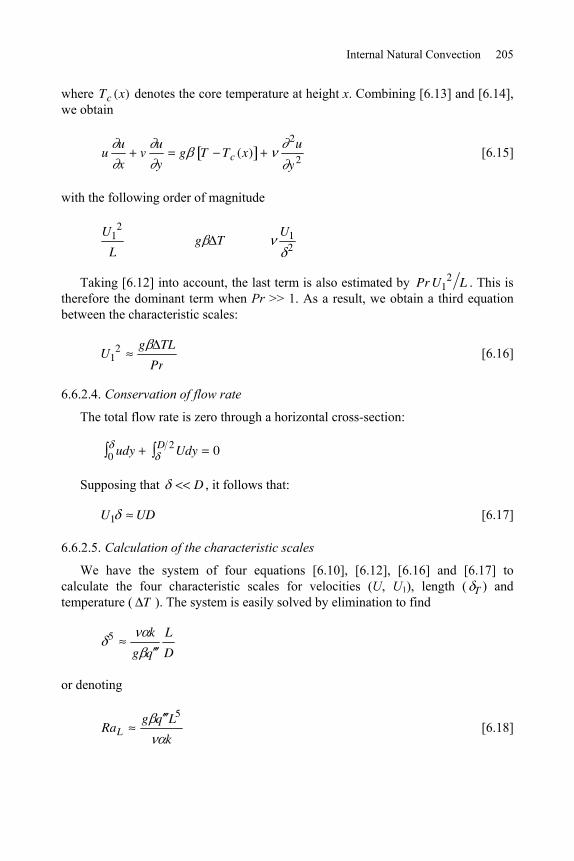
Internal Natural Convection 205
where Tc (x) denotes the core temperature at height x. Combining [6.13] and [6.14], we obtain
uu
xv
u
yg T Tc (x)
2u
y2 [6.15]
with the following order of magnitude
U12
L g T
U12
Taking [6.12] into account, the last term is also estimated by Pr U12 L . This is
therefore the dominant term when Pr >> 1. As a result, we obtain a third equation between the characteristic scales:
U12 g TL
Pr [6.16]
6.6.2.4. Conservation of flow rate
The total flow rate is zero through a horizontal cross-section:
udy0 Udy 0D 2
Supposing that D , it follows that:
U1 UD [6.17]
6.6.2.5. Calculation of the characteristic scales
We have the system of four equations [6.10], [6.12], [6.16] and [6.17] to calculate the four characteristic scales for velocities (U, U1), length ( T ) and temperature ( T ). The system is easily solved by elimination to find
5 k
g q
L
D
or denoting
RaLg q L5
k [6.18]
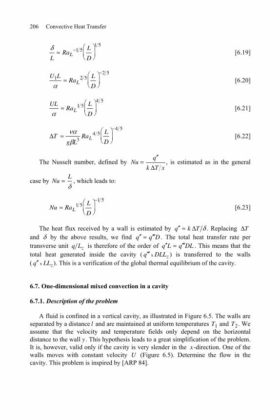
206 Convective Heat Transfer
LRaL
1 5 L
D
1 5
[6.19]
U1LRaL
2 5 L
D
2 5
[6.20]
ULRaL
1 5 L
D
4 5
[6.21]
Tg L3
RaL4 5 L
D
4 5
[6.22]
The Nusselt number, defined by Nuq
k T x, is estimated as in the general
case by NuL
, which leads to:
Nu RaL1 5 L
D
1 5
[6.23]
The heat flux received by a wall is estimated by q k T . Replacing T and by the above results, we find q q D . The total heat transfer rate per transverse unit q Lz is therefore of the order of q L q DL . This means that the total heat generated inside the cavity ( q x DLLz ) is transferred to the walls ( q x LLz ). This is a verification of the global thermal equilibrium of the cavity.
6.7. One-dimensional mixed convection in a cavity
6.7.1. Description of the problem
A fluid is confined in a vertical cavity, as illustrated in Figure 6.5. The walls are separated by a distance l and are maintained at uniform temperatures T1 and T2 . We assume that the velocity and temperature fields only depend on the horizontal distance to the wall y . This hypothesis leads to a great simplification of the problem. It is, however, valid only if the cavity is very slender in the x -direction. One of the walls moves with constant velocity U (Figure 6.5). Determine the flow in the cavity. This problem is inspired by [ARP 84].
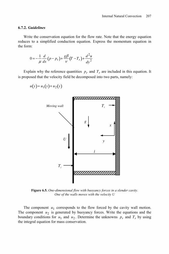
Internal Natural Convection 207
6.7.2. Guidelines
Write the conservation equation for the flow rate. Note that the energy equation reduces to a simplified conduction equation. Express the momentum equation in the form:
01 d
dxp pr
gT Tr
d 2u
dy2
Explain why the reference quantities pr and Tr are included in this equation. It is proposed that the velocity field be decomposed into two parts, namely:
u y u1 y u2 y
Moving wall
U
l
x
y
T2
g
T1
Figure 6.5. One-dimensional flow with buoyancy forces in a slender cavity. One of the walls moves with the velocity U
The component u1 corresponds to the flow forced by the cavity wall motion. The component u2 is generated by buoyancy forces. Write the equations and the boundary conditions for u1 and u2 . Determine the unknowns pr and Tr by using the integral equation for mass conservation.
208 Convective Heat Transfer
6.7.3. Solution
We suppose that the velocity u u y only depends on y because the cavity is very slender. The continuity equation then reads:
u
x
v
y
dv
dy0 [6.24]
As a result, v 0 . Otherwise, since the flow is confined in an enclosure, the integral continuity equation shows that:
udy Constant0
l0 [6.25]
The constant is obviously zero since there is no flow across the impermeable cavity walls.
We also suppose that T T y . The energy equation then reduces to the conduction equation:
uT
xv
T
y0
d 2T
dy2 [6.26]
The solution is very simple:
T T1y
lT2 T1 T1
y
lT [6.27]
The momentum equation along x yields:
01 d
dxp pr
gT Tr
d 2u
dy2 [6.28]
It is worth noting that we have kept two parameters, namely the reference pressure pr and the reference temperature Tr , in equation [6.28]. We recall that, in the classical formulation of natural convection along a vertical plate, the pressure gradient at infinity is linked to the buoyancy term at infinity, which results in the net term g T T in the momentum equation. This procedure is not valid for the confined flow of the present problem. The term d p pr dx is kept in the equation for the same reason. There is effectively a pressure gradient induced by the moving wall because this is not a simple channel Couette flow, but a confined flow in a cavity, subject to constraint [6.25].
Internal Natural Convection 209
Equation [6.28] is linear with respect to velocity. Consequently, it is possible to use a superposition method. The velocity is decomposed as:
u y u1 y u2 y
The first component u1 corresponds to the isothermal flow induced by the cavity wall motion. The component u2 is generated by buoyancy forces. The system of equations with the associated boundary conditions is:
01 d
dxp pr
d2u1
dy2
u1 0 0, u1 l U, u1 y0
ldy 0
[6.29]
0g
T Trd2u2
dy2
u2 0 0, u2 0 0, u2 y0
ldy 0
[6.30]
Integrating equation [6.29] twice and combining it with the associated boundary conditions, we obtain a velocity Couette-Poiseuille profile:
u1 yy
lU
12
l 2 d
dxp pr 1
y
l
y
l [6.31]
The unknown d p pr dx is determined by the condition u1 y0
ldy 0.
We obtain:
d
dxp pr 6
U
l 2
Thus, the component u1 y is:
u1 y U 2y
l3
y
l
2
[6.32]
210 Convective Heat Transfer
We proceed in the same way with equation [6.30] to obtain:
u2 yg Tl2 1
6y
l
y
l
3 12
T0 T1
T
y
l
y
l
2
[6.33]
The unknown T0 is deduced from the mass conservation equation u2 y0
ldy 0:
T0 T112
T [6.34]
Finally:
u2 yg Tl 2 y
l3
y
l
2
2y
l
3
[6.35]
The velocity distribution is the sum of u1 y and u2 y :
u y
U2
y
l3
y
l
2g Tl 2
U
y
l3
y
l
2
2y
l
3
[6.36]
The first component comes from forced convection and the second from natural convection. The coefficient of the second term may be rearranged in order to bring out the physical parameters as
g Tl 2
U
g Tl 3
2 UlGr Re 1
where the Grashof and Reynolds numbers are respectively
Grg Tl 3
2, Re
Ul .
It is worth noting that the dimensionless number that governs this mixed convection problem is Gr Re and not 2Gr Re , as in the general case (Chapter 5). This comes from the fact that the inertia terms are zero in the momentum equation so that the velocity contributes linearly to the viscosity term and not by its square to the inertia term.
Chapter 7
Turbulent Convection in Internal Wall Flows
7.1. Introduction
This chapter deals with internal turbulent flows in channels and ducts. The turbulence is significantly affected by the presence of the wall. The wall turbulence can be classified into two main categories. The first category deals with flows confined in space, such as turbulent flows in channels or ducts. Turbulent boundary layers constitute the second class. Both flows are similar in many aspects, especially near the wall, but there are also some significant differences between them, especially in the outer layer. Turbulent flows are of considerable industrial importance. Despite important progress made in the domain, in particular in the last four decades, turbulence still remains enigmatic in many aspects, both in the physical comprehension of the phenomena and its modeling.
7.2. Hydrodynamic stability and origin of the turbulence
One of the classical tools used to investigate the transition from laminar to turbulent flows is the theory of linear stability. The theory deals with the amplification or decay of small perturbations imposed to the basic laminar flow. If the perturbations are amplified in time and/or in space, the flow is linearly unstable and there is transition to turbulence. The hydrodynamic stability theory is an entire branch of fluid dynamics and is beyond the scope of this book. The interested reader may consult the vast literature on the subject and, for example, [DRA 81] to begin with. We restrict ourselves to a short discussion on some basic aspects of the linear stability of Poiseuille flow here.
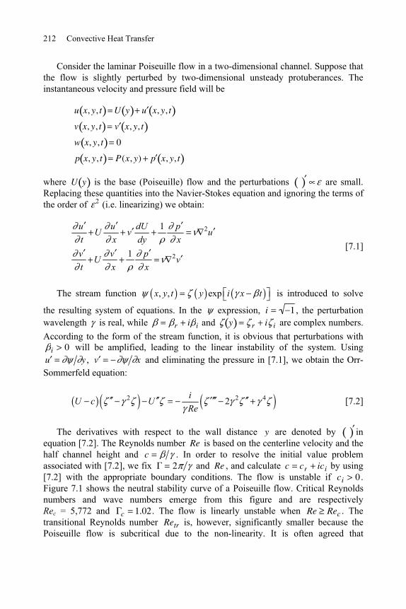
212 Convective Heat Transfer
Consider the laminar Poiseuille flow in a two-dimensional channel. Suppose that the flow is slightly perturbed by two-dimensional unsteady protuberances. The instantaneous velocity and pressure field will be
u x, y, t U y u x, y, t
v x, y, t v x, y, t
w x, y, t 0
p x, y, t P(x, y) p x, y, t
where U y is the base (Poiseuille) flow and the perturbations are small. Replacing these quantities into the Navier-Stokes equation and ignoring the terms of the order of 2 (i.e. linearizing) we obtain:
2
2
1
1
u u dU pU v u
t x dy xv v pU vt x x
[7.1]
The stream function , , expx y t y i x t is introduced to solve
the resulting system of equations. In the expression, i 1 , the perturbation wavelength is real, while r i i and y r i i are complex numbers. According to the form of the stream function, it is obvious that perturbations with
i 0 will be amplified, leading to the linear instability of the system. Using u y , v x and eliminating the pressure in [7.1], we obtain the Orr-Sommerfeld equation:
2 2 42iU c U
Re [7.2]
The derivatives with respect to the wall distance y are denoted by in equation [7.2]. The Reynolds number Re is based on the centerline velocity and the half channel height and c . In order to resolve the initial value problem associated with [7.2], we fix 2 and Re , and calculate c cr ici by using [7.2] with the appropriate boundary conditions. The flow is unstable if ci 0 . Figure 7.1 shows the neutral stability curve of a Poiseuille flow. Critical Reynolds numbers and wave numbers emerge from this figure and are respectively Rec = 5,772 and c 1.02. The flow is linearly unstable when Re Rec . The transitional Reynolds number Retr is, however, significantly smaller because the Poiseuille flow is subcritical due to the non-linearity. It is often agreed that
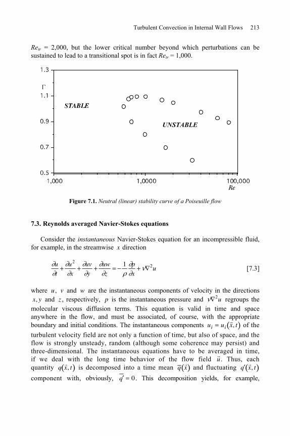
Turbulent Convection in Internal Wall Flows 213
Retr = 2,000, but the lower critical number beyond which perturbations can be sustained to lead to a transitional spot is in fact Retr = 1,000.
Figure 7.1. Neutral (linear) stability curve of a Poiseuille flow
7.3. Reynolds averaged Navier-Stokes equations
Consider the instantaneous Navier-Stokes equation for an incompressible fluid, for example, in the streamwise x direction
u
t
u2
x
uv
y
uw
z
1 p
x2u
[7.3]
where u , v and w are the instantaneous components of velocity in the directions x, y and z , respectively, p is the instantaneous pressure and 2u regroups the
molecular viscous diffusion terms. This equation is valid in time and space anywhere in the flow, and must be associated, of course, with the appropriate boundary and initial conditions. The instantaneous components ui ui x , t of the turbulent velocity field are not only a function of time, but also of space, and the flow is strongly unsteady, random (although some coherence may persist) and three-dimensional. The instantaneous equations have to be averaged in time, if we deal with the long time behavior of the flow field u . Thus, each quantity q x , t is decomposed into a time mean q x and fluctuating q x , t component with, obviously, q 0 . This decomposition yields, for example,
UNSTABLE
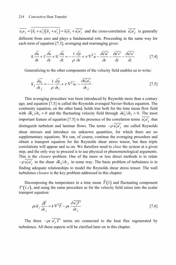
214 Convective Heat Transfer
i j i i j j i j i ju u u u u u u u u u and the cross-correlation u iu j is generally
different from zero and plays a fundamental role. Proceeding in the same way for each term of equation [7.3], averaging and rearranging gives:
u u
xv
u
yw
u
z
1 p
x2 u
u u
x
u v
y
u w
z [7.4]
Generalizing to the other components of the velocity field enables us to write:
u jui
x j
1 p
xi
2 uiu iu j
x j [7.5]
This averaging procedure was been introduced by Reynolds more than a century ago, and equation [7.5] is called the Reynolds averaged Navier-Stokes equation. The continuity equation, on the other hand, holds true both for the time mean flow field with u i xi 0 and the fluctuating velocity field through u i xi 0 . The most important feature of equation [7.5] is the presence of the correlation terms u iu j that distinguish turbulent and laminar flows. The terms u iu j are called Reynolds shear stresses and introduce six unknown quantities, for which there are no supplementary equations. We can, of course, continue the averaging procedure and obtain a transport equation for the Reynolds shear stress tensor, but then triple correlations will appear and so on. We therefore need to close the system at a given step, and the only way to proceed is to use physical or phenomenological arguments. This is the closure problem. One of the more or less direct methods is to relate
u iu j to the shear u i x j in some way. The basic problem of turbulence is in finding adequate relationships to model the Reynolds shear stress tensor. The wall turbulence closure is the key problem addressed in this chapter.
Decomposing the temperature in a time mean T x and fluctuating component T x , t , and using the same procedure as for the velocity field raises into the scalar transport equation:
cu jT
x j
k 2T cu jT
x j [7.6]
The three c u j T terms are connected to the heat flux regenerated by turbulence. All these aspects will be clarified later on in this chapter.
Turbulent Convection in Internal Wall Flows 215
7.4. Wall turbulence scaling
We will begin by introducing relevant velocity and length scales to correctly describe the physical process of the wall turbulence and wall turbulent transfer. What we mean by scaling will become progressively clearer when we introduce the notions of eddy viscosity and mixing length hypothesis. There are basically two distinct zones in a turbulent wall flow: a region next to the wall wherein the turbulence is governed by the inner scales and a zone relatively far away from the wall in which the outer scales are relevant.
The wall shear stress w u yw
and the kinematic viscosity characterize
the zone immediately adjacent to the wall. We introduce a fictitious velocity scale u w based on the shear at the wall, and which is called the shear velocity. This velocity scale well represents the wall turbulence physics since without the shear (vorticity), the turbulence cannot be sustained and w zw , where
zw u yw
, is the spanwise component of the mean vorticity field, which is
the quantity adequate near the wall. Thus, the length scale near the wall is based on the shear velocity and the viscosity and it reduces to l u . The couple u , l constitutes the inner scales (also called wall variables). A quantity q , non-dimensionalized by the inner variables, will be denoted by q , like, for example, the
mean velocity u u u , the cross-correlations u iu j u iu j u 2 , the time
t t u 2 , or the frequency f f u 2 given in wall units.
The equivalent of the wall shear stress in the context of wall heat transfer is the wall heat flux q w k T y
w. The temperature scale in inner variables can
therefore be expressed as T q wq w
kld
q w
cu , with ld u l Pr being the
diffusive length scale. We assume here that q w 0 . We will call T q w the wall flux
temperature. Note that there is a similarity between the wall shear (friction) velocity and T q w .
In duct or channel flows, the velocity scale in the outer layer is either the centerline U c or the bulk velocity U m . The length scale in this zone is obviously the half channel height e . The outer scales are the large global scales of the flow, while the inner scales are related to the local near wall phenomenology of the turbulence.
216 Convective Heat Transfer
7.5. Eddy viscosity-based one point closures
Consider the terms
2
21u vu u
u vy y yy
of the Reynolds averaged Navier-Stokes equation (called the Reynolds equation hereafter). The term u v plays the physical role of a shear stress, as indicated before, and as it is underlined in the form presented in the preceding equation. We already indicated that the Reynolds shear stress is positive in a flow where
u y 0 and that it increases the shear. We will give some qualitative arguments to show that u v 0 .
Imagine that the fluctuating wall normal velocity is v t 0 , i.e. directed towards the wall at a given time and distance y . Since v t 0 at the wall by
impermeability, it can be easily seen that locally v
y0 . We have
u
x
v
y
w
z by continuity, and if we ignore the effect of the term
w
z, we
conclude that the zones wherein v t 0 coincide with u
x0, so that globally
u t 0 and vice versa. This is, of course, a rough argument. In reality, events with u t 0 associated with v t 0 , called quadrant 1 ( Q1) events (quadrant refers here to the u v distribution), together with Q2 ( u t 0 , v t 0), Q3 ( u t 0 , v t 0) and finally Q4 ( u t 0 v t 0) events, exist altogether. However, it turns out that the contribution Q2 Q4 to the turbulent shear stress dominates, resulting in u v 0 .
The turbulent shear stress u v is added to the viscous shear stress yu to give the total shear tot . A usual and easy way to model u v is to connect it to the local u y , since the turbulence production is inconceivable without mean shear. Thus, a fictitious viscosity t y , called the eddy viscosity, is introduced. The Reynolds shear stress is consequently expressed as:
u v t yu
y [7.7]
Turbulent Convection in Internal Wall Flows 217
The eddy viscosity is certainly not a physical characteristic of the fluid. It is not a constant, but varies in space. A universal eddy viscosity formulation does not (cannot) exist since it is strongly dependent on the turbulence phenomenology. The total shear stress can now be written as:
tot tu
yy
We can at the same time introduce an eddy diffusivity to model the turbulent transfer process. The related terms of the Reynolds averaged convection equation read:
2
21v TT T
k cv Ty c y yy
The term cv T plays the physical role of a heat flux and, for the reasons given before, we obtain cv T 0 when T y 0 . Let us introduce a thermal eddy diffusivity in such a way that:
v T t y T y
The total heat flux q tot is therefore
q tot kT
ycv T c t y
T
y
in a way that is very similar to the total shear stress. Incidentally, note the sign appearing in front of q tot . This conveys the fact that the flux is conventionally opposite to the temperature gradient.
We basically distinguish two regions in the near wall turbulence, depending on whether the eddy viscosity is an order of magnitude smaller or larger than the molecular viscosity. The molecular viscosity is dominant in a thin layer adjacent to the wall wherein t y . We can expand the velocity u y into a Taylor series in this region
2 32 3
2 30 0 0
1 1 ....2 6y y y
u u uu y y y y
y y y
218 Convective Heat Transfer
and keep only the first term because of the small thickness y of this layer
u yu
y y 0
y w y
We use the wall variables ( , u ) introduced in [7.4] to write
u y y
[7.8]
for this region, commonly called the viscous sublayer. The linearity of the velocity distribution with respect to the wall normal distance is not an extraordinary result, and such a zone exists in a wall bounded laminar flow as well. The fact that the molecular viscosity is dominant in this layer does not of course mean that the flow is laminar in the viscous-sublayer: the turbulent fluctuations are very significant in this region. The non-dimensionalized turbulent fluctuation wall shear stress intensity
is for instance as large as 0.40.
Now consider the opposite case, i.e. the layer in which the eddy viscosity is dominant with t . This layer in which the direct molecular viscosity effects are negligible is relatively far away from the wall yet not too far, in such a way that the total shear stress tot remains approximately constant and equal to the wall shear stress w at the wall (Figure 7.2). This is why this region is also called the constant stress sublayer. These hypotheses lead to:
tot w t y u y
The eddy viscosity t y remains to be modeled. Dimensional analysis enables us to write t (y) v , where and v are respectively the length and velocity scales characterizing the turbulent mixing. The natural choice for v in the inner layer is the wall shear stress velocity u . The length scale of the eddy viscosity, in return is the wall normal distance y to the wall. The turbulent mixing becomes progressively important as we move off the wall and y where is a constant. The turbulence closures are generally based on phenomenological arguments. The flow quantities modeled this way have to be subsequently confronted to the experiments or the direct numerical simulations when available. There is no universal and general approach to the problem. The closure y , where 0.40 is the universal von Karman constant, and is one of the historical propositions in the domain.
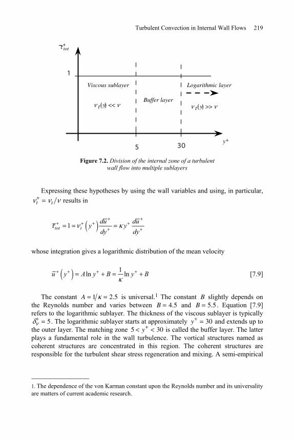
Turbulent Convection in Internal Wall Flows 219
5 30y+
1
tot +
Viscous sublayer Logarithmic layer
Buffer layer t y << t y >>
Figure 7.2. Division of the internal zone of a turbulent wall flow into multiple sublayers
Expressing these hypotheses by using the wall variables and using, in particular,
t t results in
1tot tdu du
y ydy dy
whose integration gives a logarithmic distribution of the mean velocity
1ln lnu y A y B y B
[7.9]
The constant A 1 2.5 is universal.1 The constant B slightly depends on the Reynolds number and varies between B 4.5 and B 5.5 . Equation [7.9] refers to the logarithmic sublayer. The thickness of the viscous sublayer is typically
5 . The logarithmic sublayer starts at approximately y 30 and extends up to the outer layer. The matching zone 5 y 30 is called the buffer layer. The latter plays a fundamental role in the wall turbulence. The vortical structures named as coherent structures are concentrated in this region. The coherent structures are responsible for the turbulent shear stress regeneration and mixing. A semi-empirical
1. The dependence of the von Karman constant upon the Reynolds number and its universality are matters of current academic research.
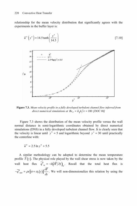
220 Convective Heat Transfer
relationship for the mean velocity distribution that significantly agrees with the experiments in the buffer layer is:
14.5 tanh14.5y
u y
[7.10]
Figure 7.3. Mean velocity profile in a fully developed turbulent channel flow inferred from direct numerical simulations at Re u h 180 [DOC 06]
Figure 7.3 shows the distribution of the mean velocity profile versus the wall normal distance in semi-logarithmic coordinates obtained by direct numerical simulations (DNS) in a fully developed turbulent channel flow. It is clearly seen that the velocity is linear until y 5 and logarithmic beyond y 30 until practically the centerline with:
u 2.5 ln y 5.5
A similar methodology can be adopted to determine the mean temperature profile T y . The physical role played by the wall shear stress is now taken by the wall heat flux q w k T y
w. Recall that the total heat flux is
q tot c t yT
y. We will non-dimensionalize this relation by using the
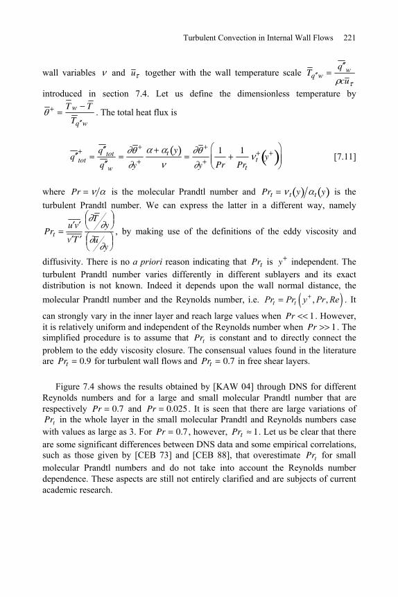
Turbulent Convection in Internal Wall Flows 221
wall variables and u together with the wall temperature scale T q wq w
cu
introduced in section 7.4. Let us define the dimensionless temperature by T w T
T q w
. The total heat flux is
q totq tot
q w y
t y
y
1
Pr
1
Prtt y
[7.11]
where Pr is the molecular Prandtl number and Prt t y t y is the turbulent Prandtl number. We can express the latter in a different way, namely
Prtu v
v T
T y
u y
, by making use of the definitions of the eddy viscosity and
diffusivity. There is no a priori reason indicating that Prt is y independent. The turbulent Prandtl number varies differently in different sublayers and its exact distribution is not known. Indeed it depends upon the wall normal distance, the molecular Prandtl number and the Reynolds number, i.e. , ,t tPr Pr y Pr Re . It
can strongly vary in the inner layer and reach large values when Pr 1 . However, it is relatively uniform and independent of the Reynolds number when Pr 1 . The simplified procedure is to assume that Prt is constant and to directly connect the problem to the eddy viscosity closure. The consensual values found in the literature are Prt 0.9 for turbulent wall flows and Prt 0.7 in free shear layers.
Figure 7.4 shows the results obtained by [KAW 04] through DNS for different Reynolds numbers and for a large and small molecular Prandtl number that are respectively Pr 0.7 and Pr 0.025 . It is seen that there are large variations of Prt in the whole layer in the small molecular Prandtl and Reynolds numbers case with values as large as 3. For Pr 0.7 , however, Prt 1. Let us be clear that there are some significant differences between DNS data and some empirical correlations, such as those given by [CEB 73] and [CEB 88], that overestimate Prt for small molecular Prandtl numbers and do not take into account the Reynolds number dependence. These aspects are still not entirely clarified and are subjects of current academic research.
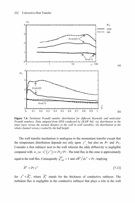
222 Convective Heat Transfer
100101.10
1
2
3
4
1020180
Prt
y+
Re
Pr=0.71
Pr=0.025
(a)
1.0.90.80.70.60.50.40.30.20.10.0
1
2
3
4Prt
Pr=0.71
Pr=0.025
yh
(b)
Figure 7.4. Turbulent Prandtl number distribution for different Reynolds and molecular Prandtl numbers. Data adapted from DNS conducted by [KAW 04]: (a) distribution in the inner layer versus the normal distance to the wall in wall variables; (b) distribution in the whole channel versus y scaled by the half height
The wall transfer mechanism is analogous to the momentum transfer except that the temperature distribution depends not only upon y , but also on Pr and Prt . Consider a first sublayer next to the wall wherein the eddy diffusivity is negligible compared with , i.e. t ty Pr Pr . The total flux in this zone is approximately
equal to the wall flux. Consequently q tot 1 and d dy Pr , implying
Pr y [7.12]
for y c , where c stands for the thickness of conductive sublayer. The turbulent flux is negligible in the conductive sublayer that plays a role in the wall
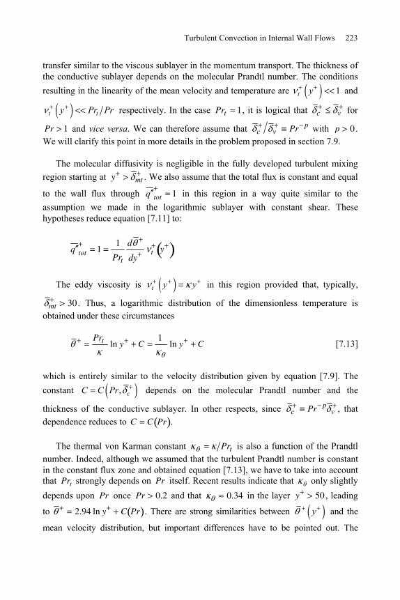
Turbulent Convection in Internal Wall Flows 223
transfer similar to the viscous sublayer in the momentum transport. The thickness of the conductive sublayer depends on the molecular Prandtl number. The conditions resulting in the linearity of the mean velocity and temperature are 1t y
and
t ty Pr Pr respectively. In the case Prt 1, it is logical that c v for
Pr 1 and vice versa. We can therefore assume that c v Pr p with p 0 . We will clarify this point in more details in the problem proposed in section 7.9.
The molecular diffusivity is negligible in the fully developed turbulent mixing region starting at y mt . We also assume that the total flux is constant and equal
to the wall flux through q tot 1 in this region in a way quite similar to the assumption we made in the logarithmic sublayer with constant shear. These hypotheses reduce equation [7.11] to:
q tot 11
Prt
d
dyt y
The eddy viscosity is t y y in this region provided that, typically,
mt 30 . Thus, a logarithmic distribution of the dimensionless temperature is obtained under these circumstances
Prt ln y C1
ln y C
[7.13]
which is entirely similar to the velocity distribution given by equation [7.9]. The constant , cC C Pr depends on the molecular Prandtl number and the
thickness of the conductive sublayer. In other respects, since c Pr pv , that
dependence reduces to C C Pr .
The thermal von Karman constant Prt is also a function of the Prandtl number. Indeed, although we assumed that the turbulent Prandtl number is constant in the constant flux zone and obtained equation [7.13], we have to take into account that Prt strongly depends on Pr itself. Recent results indicate that only slightly depends upon Pr once Pr 0.2 and that 0.34 in the layer y 50 , leading
to 2.94 ln y C Pr . There are strong similarities between y and the
mean velocity distribution, but important differences have to be pointed out. The
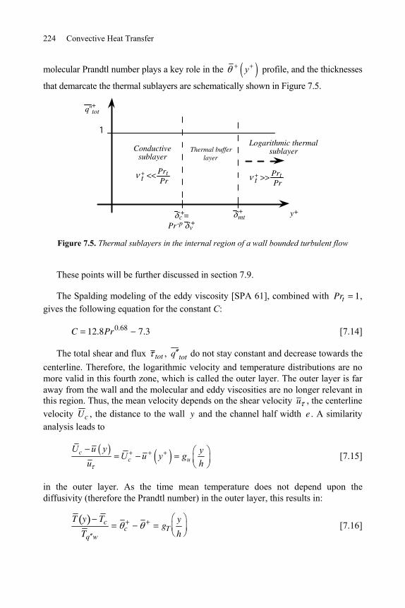
224 Convective Heat Transfer
molecular Prandtl number plays a key role in the y profile, and the thicknesses
that demarcate the thermal sublayers are schematically shown in Figure 7.5.
y+
1
Conductive sublayer
Thermal buffer layer
t+ << Prt
Pr
Logarithmic thermal sublayer
t+ >> Prt
Pr
c +=
Pr -p v +
mt +
q"tot +
Figure 7.5. Thermal sublayers in the internal region of a wall bounded turbulent flow
These points will be further discussed in section 7.9.
The Spalding modeling of the eddy viscosity [SPA 61], combined with Prt 1, gives the following equation for the constant C:
C 12.8Pr0.68 7.3 [7.14]
The total shear and flux tot , q tot do not stay constant and decrease towards the centerline. Therefore, the logarithmic velocity and temperature distributions are no more valid in this fourth zone, which is called the outer layer. The outer layer is far away from the wall and the molecular and eddy viscosities are no longer relevant in this region. Thus, the mean velocity depends on the shear velocity u , the centerline velocity U c , the distance to the wall y and the channel half width e . A similarity analysis leads to
cc u
U u y yU u y g
u h [7.15]
in the outer layer. As the time mean temperature does not depend upon the diffusivity (therefore the Prandtl number) in the outer layer, this results in:
T y T cT q w
c gTy
h [7.16]
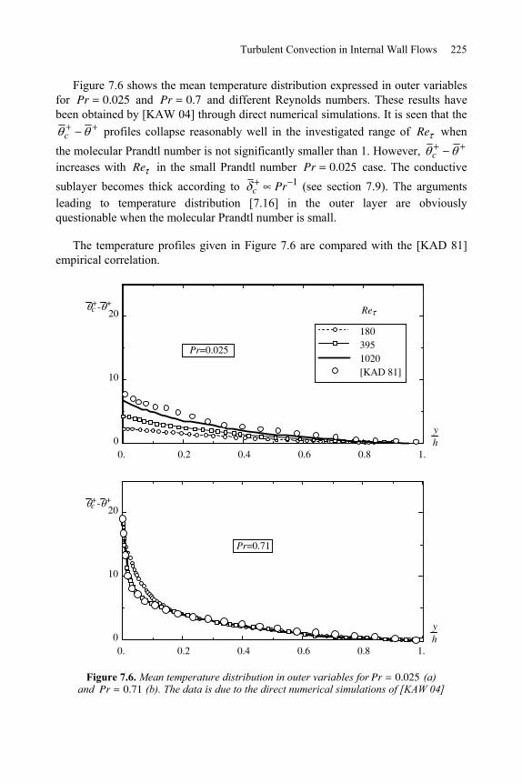
Turbulent Convection in Internal Wall Flows 225
Figure 7.6 shows the mean temperature distribution expressed in outer variables for Pr 0.025 and Pr 0.7 and different Reynolds numbers. These results have been obtained by [KAW 04] through direct numerical simulations. It is seen that the
c profiles collapse reasonably well in the investigated range of Re when the molecular Prandtl number is not significantly smaller than 1. However, c increases with Re in the small Prandtl number Pr 0.025 case. The conductive sublayer becomes thick according to c Pr 1 (see section 7.9). The arguments leading to temperature distribution [7.16] in the outer layer are obviously questionable when the molecular Prandtl number is small.
The temperature profiles given in Figure 7.6 are compared with the [KAD 81] empirical correlation.
1.0.80.60.40.20.0
10
20
1803951020[KAD 81]
yh
c+- +
Pr=0.025
Re
1.0.80.60.40.20.0
10
20
yh
c+- +
Pr=0.71
Figure 7.6. Mean temperature distribution in outer variables for Pr 0.025 (a) and Pr 0.71 (b). The data is due to the direct numerical simulations of [KAW 04]
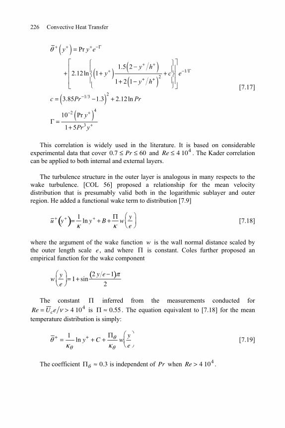
226 Convective Heat Transfer
1/2
21/3
42
3
Pr
1.5 22.12ln 1
1 2 1
3.85 1.3 2.12 ln
10 Pr
1 5
y y e
y hy c e
y h
c Pr Pr
y
Pr y
[7.17]
This correlation is widely used in the literature. It is based on considerable experimental data that cover 0.7 Pr 60 and Re 4 104 . The Kader correlation can be applied to both internal and external layers.
The turbulence structure in the outer layer is analogous in many respects to the wake turbulence. [COL 56] proposed a relationship for the mean velocity distribution that is presumably valid both in the logarithmic sublayer and outer region. He added a functional wake term to distribution [7.9]
u y1
ln y B wy
e [7.18]
where the argument of the wake function w is the wall normal distance scaled by the outer length scale e , and where is constant. Coles further proposed an empirical function for the wake component
wy
e1 sin
2 y e 1
2
The constant inferred from the measurements conducted for Re U ce 4 104 is 0.55 . The equation equivalent to [7.18] for the mean temperature distribution is simply:
1ln y C w
y
e [7.19]
The coefficient 0.3 is independent of Pr when Re 4 104 .
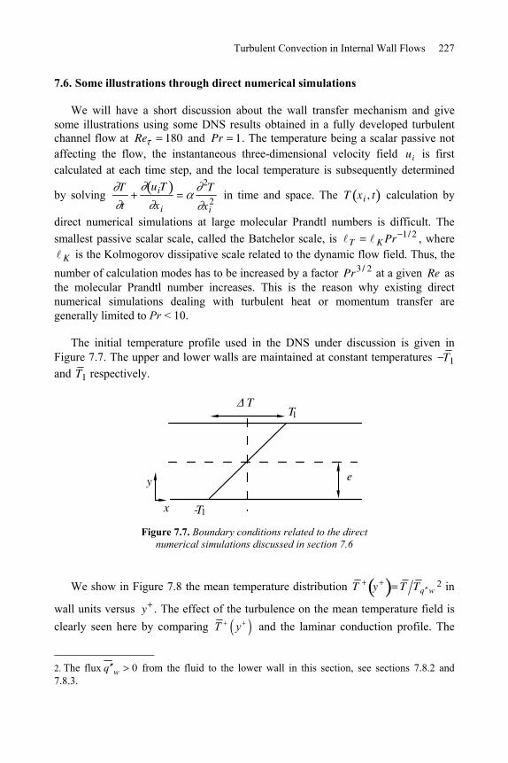
Turbulent Convection in Internal Wall Flows 227
7.6. Some illustrations through direct numerical simulations
We will have a short discussion about the wall transfer mechanism and give some illustrations using some DNS results obtained in a fully developed turbulent channel flow at Re 180 and Pr 1. The temperature being a scalar passive not affecting the flow, the instantaneous three-dimensional velocity field ui is first calculated at each time step, and the local temperature is subsequently determined
by solving T
t
uiT
xi
2T
xi2
in time and space. The T xi , t calculation by
direct numerical simulations at large molecular Prandtl numbers is difficult. The smallest passive scalar scale, called the Batchelor scale, is T K Pr 1/ 2 , where
K is the Kolmogorov dissipative scale related to the dynamic flow field. Thus, the number of calculation modes has to be increased by a factor Pr3 / 2 at a given Re as the molecular Prandtl number increases. This is the reason why existing direct numerical simulations dealing with turbulent heat or momentum transfer are generally limited to Pr < 10.
The initial temperature profile used in the DNS under discussion is given in Figure 7.7. The upper and lower walls are maintained at constant temperatures T 1 and T 1 respectively.
T1
-T1
y
x
e
T
Figure 7.7. Boundary conditions related to the direct
numerical simulations discussed in section 7.6
We show in Figure 7.8 the mean temperature distribution T y T T q w2 in
wall units versus y . The effect of the turbulence on the mean temperature field is clearly seen here by comparing T y and the laminar conduction profile. The
2. The flux q w 0 from the fluid to the lower wall in this section, see sections 7.8.2 and 7.8.3.
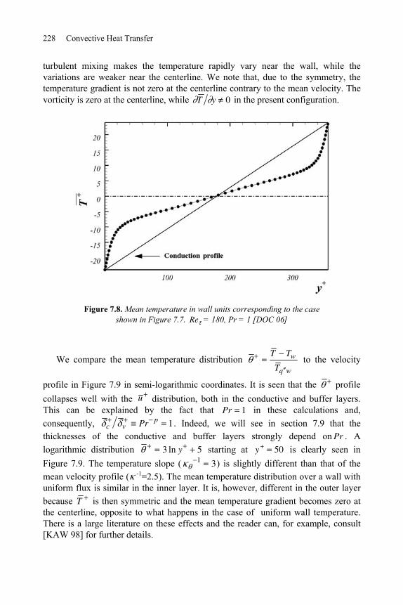
228 Convective Heat Transfer
turbulent mixing makes the temperature rapidly vary near the wall, while the variations are weaker near the centerline. We note that, due to the symmetry, the temperature gradient is not zero at the centerline contrary to the mean velocity. The vorticity is zero at the centerline, while T y 0 in the present configuration.
Figure 7.8. Mean temperature in wall units corresponding to the case shown in Figure 7.7. Re = 180, Pr = 1 [DOC 06]
We compare the mean temperature distribution T Tw
T q w
to the velocity
profile in Figure 7.9 in semi-logarithmic coordinates. It is seen that the profile collapses well with the u distribution, both in the conductive and buffer layers. This can be explained by the fact that Pr 1 in these calculations and, consequently, c v Pr p 1 . Indeed, we will see in section 7.9 that the thicknesses of the conductive and buffer layers strongly depend on Pr . A logarithmic distribution 3 ln y 5 starting at y 50 is clearly seen in Figure 7.9. The temperature slope ( 1 3) is slightly different than that of the mean velocity profile ( -1=2.5). The mean temperature distribution over a wall with uniform flux is similar in the inner layer. It is, however, different in the outer layer because T is then symmetric and the mean temperature gradient becomes zero at the centerline, opposite to what happens in the case of uniform wall temperature. There is a large literature on these effects and the reader can, for example, consult [KAW 98] for further details.
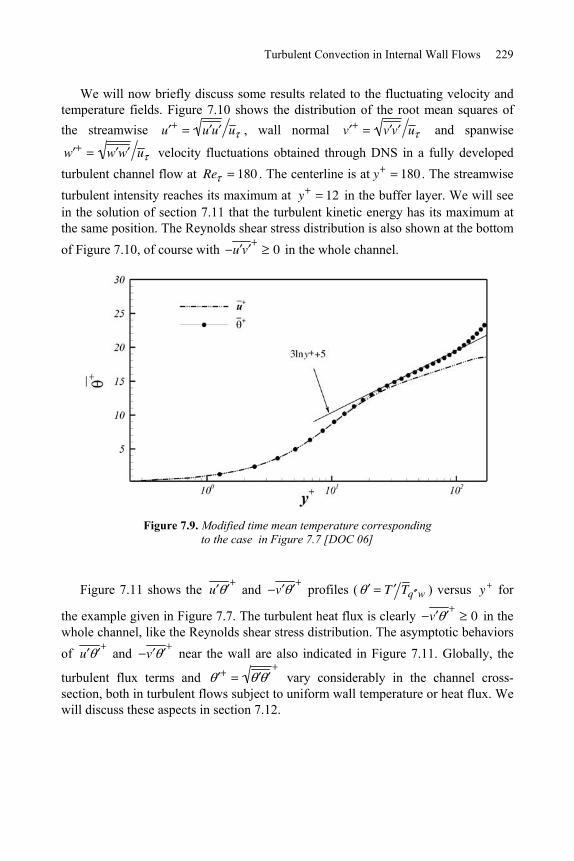
Turbulent Convection in Internal Wall Flows 229
We will now briefly discuss some results related to the fluctuating velocity and temperature fields. Figure 7.10 shows the distribution of the root mean squares of the streamwise u u u u , wall normal v v v u and spanwise
w w w u velocity fluctuations obtained through DNS in a fully developed turbulent channel flow at Re 180 . The centerline is at y 180 . The streamwise turbulent intensity reaches its maximum at y 12 in the buffer layer. We will see in the solution of section 7.11 that the turbulent kinetic energy has its maximum at the same position. The Reynolds shear stress distribution is also shown at the bottom of Figure 7.10, of course with u v 0 in the whole channel.
Figure 7.9. Modified time mean temperature corresponding
to the case in Figure 7.7 [DOC 06]
Figure 7.11 shows the u and v profiles ( T T q w ) versus y for
the example given in Figure 7.7. The turbulent heat flux is clearly v 0 in the whole channel, like the Reynolds shear stress distribution. The asymptotic behaviors of u and v near the wall are also indicated in Figure 7.11. Globally, the
turbulent flux terms and vary considerably in the channel cross-section, both in turbulent flows subject to uniform wall temperature or heat flux. We will discuss these aspects in section 7.12.
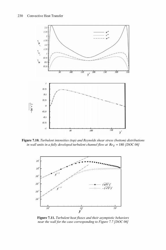
230 Convective Heat Transfer
Figure 7.10. Turbulent intensities (top) and Reynolds shear stress (bottom) distributions in wall units in a fully developed turbulent channel flow at Re 180 [DOC 06]
Figure 7.11. Turbulent heat fluxes and their asymptotic behaviors near the wall for the case corresponding to Figure 7.7 [DOC 06]
Turbulent Convection in Internal Wall Flows 231
7.7. Empirical correlations
We will give some empirical correlations relating the Nusselt number to the Reynolds and Prandtl numbers in this section. The Nusselt number is defined by
Nuq w
k T w T m Dh
where it is recalled that Dh is the hydraulic diameter and T m is the bulk temperature. The Reynolds number is based on the bulk velocity U m and the hydraulic diameter, i.e. ReDh U m Dh . Remember that the Darcy-Weisbach drag
coefficient is w1
8U m
2 and that the pressure loss for a duct of length L in the
fully developed regime is:
p* 1
2U m
2 L
Dh
The Blasius empiric correlation for is:
0.3164
ReDh0.25
ReDh 105
[7.20]
This correlation is valid for a developed turbulent flow over smooth walls. For rough walls, in particular in the presence of sand roughness of typical height3 ks , we often use the Nikuradse law:
12 log10
ks Dh
3.7
2.51
ReDh [7.21]
The existing empirical correlations for the heat transfer often refer to fully developed turbulent flows over smooth walls. For instance, the Dittus-Boelter correlation is quite popular:
Nu 0.0243Pr0.4ReDh0.8
[7.22]
3. Do not confuse ks with the conductivity.
232 Convective Heat Transfer
It has the advantage of being simple and quite precise in the range:
0.7 Pr 160 Re 104
The Karman-Boelter-Martinelli correlation
NuReDhPr 8
0.833 5Pr 5 ln 5Pr 1 2.5 ln ReDh 8 60
[7.23]
was originally obtained in a turbulent pipe flow under uniform wall heat flux. It corresponds well to the eddy diffusivity predictions for Pr 0.7 [CEB 88]. The Sleicher and Rouse correlation is recommended for liquid metals ( Pr 1)
Nu 6.3 0.0167ReDh0.85Pr0.93
[7.24]
for fully developed turbulent pipe flows under constant wall flux. We recommend the Kader and Yaglom correlation be used in internal turbulent wall flows subject to constant temperature at the wall
NuReDhPr 2
4.24 ln ReDh /16 25 Pr2 / 3 4.24 ln Pr 20.2
[7.25]
in the range 1 Pr 106 and 104 ReDh 106.
A useful correlation of acceptable precision between the Stanton number defined as
Sth
cU m
q w
cU m T w T m
and the drag coefficient,4 C f w U m2 , is the Colburn relationship
St C f Pr2 / 3 [7.26]
Note that Nu St Re Pr according to the definitions of these dimensionless parameters. 4. Cf is often given in the literature in the form scaled by 1 2 U m
2 .
Turbulent Convection in Internal Wall Flows 233
These relationships can be applied as a first approximation to fully developed turbulent flows in ducts of arbitrary sections by using the hydraulic diameter definition.
The effect of the wall roughness has to be analyzed separately. Some indications are given in Chapter 8. The reader may consult [WEB 05] for correlations in turbulent flows over rough walls.
7.8. Exact relations for a fully developed turbulent channel flow
7.8.1. Reynolds shear stress
We will obtain three precise relations that govern the heat transfer process in the three following problems. We begin, first, by establishing a precise equation for the Reynolds shear stress distribution that is also often used to check the quality of the experimental data or the convergence of direct numerical simulations.
7.8.1.1. Reynolds shear stress in a fully developed turbulent channel flow. Description of the problem
The aim is to show that the total shear stress (i.e. the sum of turbulent and viscous stresses) varies linearly with the distance to the wall in a fully developed steady turbulent channel flow that is homogenous in the streamwise and spanwise directions.
7.8.1.2. Guidelines
The flow is homogenous in the streamwise (longitudinal) and spanwise directions. The first step is to determine the exact relationship that governs the mean velocity that has to be subsequently analyzed to find out the time-mean pressure gradient and the required equation for the Reynolds shear stress.
7.8.1.3. Solution
The homogenity in the streamwise x and spanwise z directions implies x z 0 . The time-mean spanwise velocity is consequently w 0 . The
continuity therefore leads to v 0 and u u y . The precise Reynolds equations in the streamwise and wall normal directions read:
2
210
10
p u u vx yy
p v vy y
[7.27]
234 Convective Heat Transfer
It is seen that the pressure p depends not only upon x , but that there is also a wall normal distance dependence induced by the v v gradient. The integration of the second equation given above from the wall y 0 to a point y in the flow leads to
0 0
1y y
p v vdy dy v v y
y y
and, consequently, p x, y v v y p0 x where p 0 x is the pressure at the
wall. Therefore, and since v v depends only on y , we have 0dppx dx
by
homogenity.
Thus, at this step it is straightforward to integrate the u y equation from the wall to the channel centerline y e. Noticing that the shear u y
y e0 , we
obtain
01 dp 0
dxe
1w
because, by symmetry, the Reynolds shear stress u v is zero both at the wall and at the centerline. The last equation connects the pressure gradient dp 0 dx to the wall shear stress w u y y 0 . The use of the last relationship in the u
equation and the integration of the latter from the wall to y lead to
u
yy u v y w 1
y
e
wherein the total shear stress clearly appears at the right hand side, i.e.
totu
yy u v y
which is the sum of the viscous and Reynolds shear stresses. Scaling this equation by the inner variables (based on the length and velocity scales that are respectively u and l u ) results in the simple equation:
totu
yu v 1
y
e [7.28]
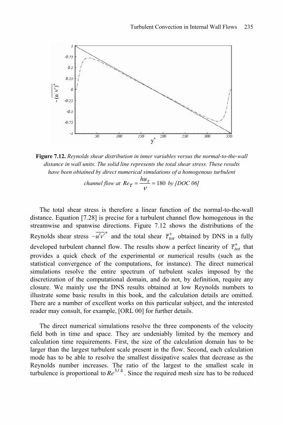
Turbulent Convection in Internal Wall Flows 235
Figure 7.12. Reynolds shear distribution in inner variables versus the normal-to-the-wall distance in wall units. The solid line represents the total shear stress. These results
have been obtained by direct numerical simulations of a homogenous turbulent
channel flow at Rehu
180 by [DOC 06]
The total shear stress is therefore a linear function of the normal-to-the-wall distance. Equation [7.28] is precise for a turbulent channel flow homogenous in the streamwise and spanwise directions. Figure 7.12 shows the distributions of the Reynolds shear stress u v and the total shear tot obtained by DNS in a fully developed turbulent channel flow. The results show a perfect linearity of tot that provides a quick check of the experimental or numerical results (such as the statistical convergence of the computations, for instance). The direct numerical simulations resolve the entire spectrum of turbulent scales imposed by the discretization of the computational domain, and do not, by definition, require any closure. We mainly use the DNS results obtained at low Reynolds numbers to illustrate some basic results in this book, and the calculation details are omitted. There are a number of excellent works on this particular subject, and the interested reader may consult, for example, [ORL 00] for further details.
The direct numerical simulations resolve the three components of the velocity field both in time and space. They are undeniably limited by the memory and calculation time requirements. First, the size of the calculation domain has to be larger than the largest turbulent scale present in the flow. Second, each calculation mode has to be able to resolve the smallest dissipative scales that decrease as the Reynolds number increases. The ratio of the largest to the smallest scale in turbulence is proportional to Re3 / 4 . Since the required mesh size has to be reduced
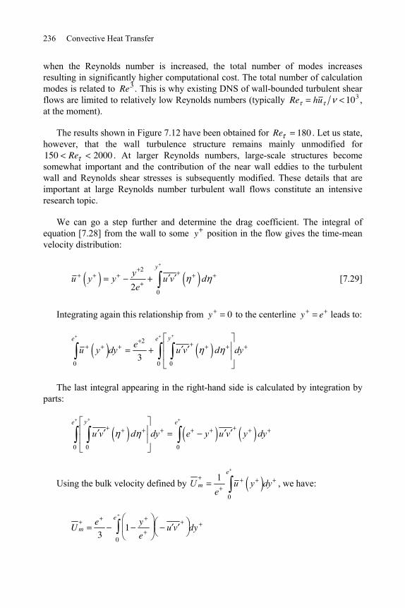
236 Convective Heat Transfer
when the Reynolds number is increased, the total number of modes increases resulting in significantly higher computational cost. The total number of calculation modes is related to Re3 . This is why existing DNS of wall-bounded turbulent shear flows are limited to relatively low Reynolds numbers (typically Re hu 103 , at the moment).
The results shown in Figure 7.12 have been obtained for Re 180 . Let us state, however, that the wall turbulence structure remains mainly unmodified for 150 Re 2000 . At larger Reynolds numbers, large-scale structures become somewhat important and the contribution of the near wall eddies to the turbulent wall and Reynolds shear stresses is subsequently modified. These details that are important at large Reynolds number turbulent wall flows constitute an intensive research topic.
We can go a step further and determine the drag coefficient. The integral of equation [7.28] from the wall to some y position in the flow gives the time-mean velocity distribution:
2
02
yy
u y y u v de
[7.29]
Integrating again this relationship from y 0 to the centerline y e leads to:
2
0 0 03
ye ee
u y dy u v d dy
The last integral appearing in the right-hand side is calculated by integration by parts:
0 0 0
ye e
u v d dy e y u v y dy
Using the bulk velocity defined by 0
1e
mU u y dye
, we have:
U me
31
y
e0
e
u v dy
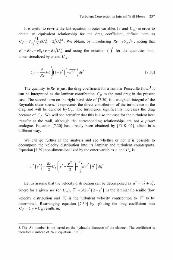
Turbulent Convection in Internal Wall Flows 237
It is useful to rewrite the last equation in outer variables ( e and U m ) in order to obtain an equivalent relationship for the drag coefficient, defined here as
C f w1
2U m
2 2 U m2 . We obtain, by introducing Re eU m , noting that
e Re eu Re U m and using the notation * for the quantities non-dimensionalized by e and U m :
1** *
0
6 6 1fC y u v dyRe
[7.30]
The quantity 6 Re is just the drag coefficient for a laminar Poiseuille flow.5 It can be interpreted as the laminar contribution C fl to the total drag in the present case. The second term on the right-hand side of [7.30] is a weighted integral of the Reynolds shear stress. It represents the direct contribution of the turbulence to the drag and will be denoted by C ft . The turbulence significantly increases the drag because of C ft . We will see hereafter that this is also the case for the turbulent heat transfer at the wall, although the corresponding relationships are not a priori analogue. Equation [7.30] has already been obtained by [FUK 02], albeit in a different way.
We can go further in the analysis and see whether or not it is possible to decompose the velocity distribution into its laminar and turbulent counterparts. Equation [7.29] non-dimensionalized by the outer variables e and U m is:
**2 ** * * * *
02 2
y
fRe y
u y C y u v d
Let us assume that the velocity distribution can be decomposed as u * u l* u t
*,
where for a given Re (or U m ), * * *3 2 2lu y y is the laminar Poiseuille flow
velocity distribution and u t* is the turbulent velocity contribution to u * to be
determined. Rearranging equation [7.30] by splitting the drag coefficient into C f C fl C ft results in:
5. The Re number is not based on the hydraulic diameter of the channel. The coefficient is therefore 6 instead of 24 in equation [7.30].
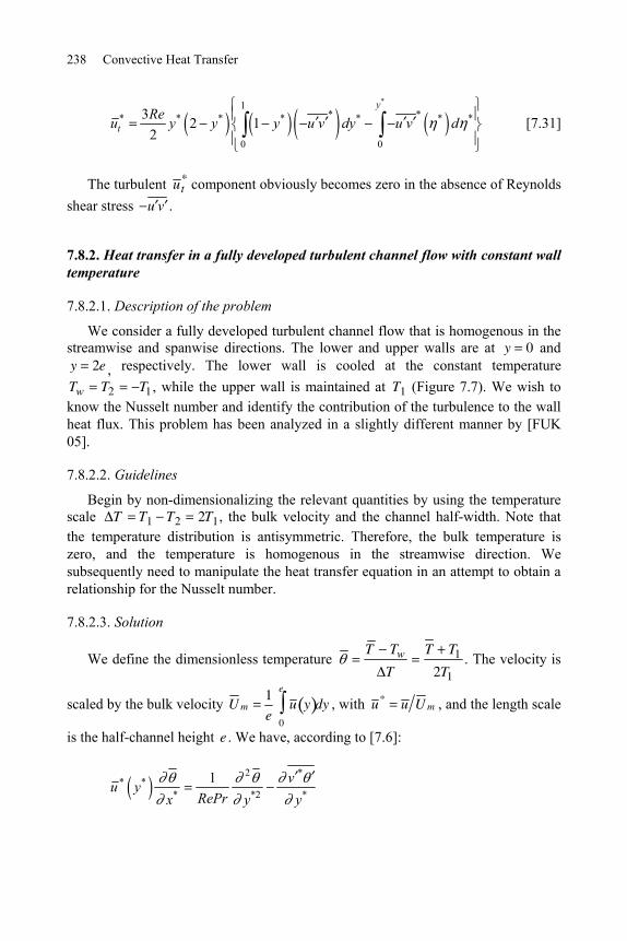
238 Convective Heat Transfer
*1* ** * * * * * *
0 0
3 2 12
y
tRe
u y y y u v dy u v d
[7.31]
The turbulent u t* component obviously becomes zero in the absence of Reynolds
shear stress u v .
7.8.2. Heat transfer in a fully developed turbulent channel flow with constant wall temperature
7.8.2.1. Description of the problem
We consider a fully developed turbulent channel flow that is homogenous in the streamwise and spanwise directions. The lower and upper walls are at y 0 and y 2e , respectively. The lower wall is cooled at the constant temperature Tw T2 T1 , while the upper wall is maintained at T1 (Figure 7.7). We wish to know the Nusselt number and identify the contribution of the turbulence to the wall heat flux. This problem has been analyzed in a slightly different manner by [FUK 05].
7.8.2.2. Guidelines
Begin by non-dimensionalizing the relevant quantities by using the temperature scale T T1 T2 2T1, the bulk velocity and the channel half-width. Note that the temperature distribution is antisymmetric. Therefore, the bulk temperature is zero, and the temperature is homogenous in the streamwise direction. We subsequently need to manipulate the heat transfer equation in an attempt to obtain a relationship for the Nusselt number.
7.8.2.3. Solution
We define the dimensionless temperature T Tw
T
T T1
2T1. The velocity is
scaled by the bulk velocity U m1e
u y0
e
dy , with u * u U m , and the length scale
is the half-channel height e . We have, according to [7.6]:
2 ** *
* *2 *1 v
u yRePrx y y
Turbulent Convection in Internal Wall Flows 239
The corresponding boundary conditions are * 0 0y and * 2 1y . The integration of this relationship from the lower to the upper wall yields
d
dx*u * dy*
0
22
d m
dx*1
RePr y*y* 2 y*
y* 0
0
due to the antisymmetry. Thus, not only the bulk temperature m is constant, but also m 0 , because the velocity distribution is symmetric, while the temperature profile
is antisymmetric with respect to the channel centerline. The energy budget clearly indicates that x* 0 . Hence, the transport equation takes the simple form:
01
RePr
2
y*2
v *
y*
[7.32]
The temperature profile in the related laminar flow ( v * 0 ) reduces to the simple linear conduction distribution. The integration of the preceding equation from the upper wall to y* somewhere in the flow results in:
1
RePr y*y* 0
Nu
RePr
1
RePr y*v *
[7.33]
The Nusselt number is defined by * *
* *0 2y y
Nu y y . The
global transfer process is governed by the following equation obtained by the integral of the local equation [7.33] from the upper wall to the centerline y* 1
Nu 1 RePr v * '0
1dy*
[7.34]
wherein we made use of the boundary condition y 0 0 and the antisymmetry
at the centerline through * 1 1y . Equation [7.34] is exact; it does not
necessitate any closure and it is instructive in several aspects. It is to be noted that the Nusselt number is simply Nul 1 in the absence of turbulent flux terms, which is the Nu of the related laminar flow in the same configuration. It is clearly seen that the Nusselt number can easily be decomposed into two parts, namely
Nut Nul Numt , where Numt RePr v * '0
1dy* stays for the turbulent mixing
contribution.
240 Convective Heat Transfer
The turbulence considerably increases the wall transfer since v ' 0 . It is important to note that equations [7.34] and [7.30], which correspond respectively to heat and momentum transfer processes, are different. The contribution of the turbulence to mixing is a simple integral of v * ' while the u v
* contribution to the drag coefficient is a weighted integral.
7.8.3. Heat transfer in a fully developed turbulent channel flow with uniform wall heat flux
7.8.3.1. Description of the problem
The problem is identical to that in section 7.8.2, but with different boundary conditions. The channel is now subject to constant uniform heat flux q w
6 of the same intensity on the upper and lower walls.
7.8.3.2. Guidelines
Both the upper and lower walls are maintained at the same heat flux; the wall temperature T w(x) varies linearly with x in the same way as the bulk temperature,
as well as T x, y , in the fully developed thermal regime (dT wdx
dT mdx
T x, y
x).
The energy budget in the channel is obtained by integrating the convection equation from the lower to the upper wall y 2e
d
dxu
0
2eT dy
dT wdx
u0
2edy
T
y 0
2e
v T 0
2e 2q w
c
because u does not depend upon x . That results in dT w dx q w ceU m , suggesting the use of the temperature scale T e dT w dx q w cU m . We therefore propose to formulate the problem by using the dimensionless temperature
T w x T x, y
T. The transport equation has to be integrated in a second step in
a way similar to that in section 7.8.2.3 with the aim of determining the turbulence contribution to the Nusselt number. Note that the boundary conditions here are
* 0 0y and * 2 0y .
6. q w is positive from the wall to the fluid in the channel.
Turbulent Convection in Internal Wall Flows 241
7.8.3.3. Solution
The temperature scale suggested above gives rise to the non-dimensionalized transport equation
u *
T
dT wdx*
u *1
RePr
d2
dy*2dv *
dy*
[7.35]
where we used the outer scales e and U m to obtain dimensionless parameters noted by *, in a way very similar to that in section 7.8.2.3. A first integration of the last equation from the lower wall to the channel centerline yields
01
RePr
d
dy*y* 0
1
since the temperature profile is symmetric; therefore, *
*1
0y
d dy and the
integral of the left-hand side of [7.35] is 1, due directly to the definition of the bulk velocity. The Nusselt number based on the bulk temperature and the half height of
the channel is Nu1
m
d
dy*y* 0
, with the dimensionless bulk temperature
mT w x T m x
T. Using [7.35] results in Nu
RePr
m
.
The rest of the solution is very similar to the procedure used in section 7.8.1.3. A first integration of equation [7.35] enables us to obtain a relationship establishing equilibrium between different flux terms:
*
* * * * **
0
1 1y
du d y v y
RePr dy [7.36]
Let us denote u *d *
0
y*
by y* u *d *
0
y*
. The temperature field is calculated
by integrating [7.36] from the wall to y*
* *
* * * * * * *
0 0
1y y
d y y v dRePr
242 Convective Heat Transfer
and using the boundary condition 0 0 . We proceed by weighting this equation
by the velocity *u y
*
*
* * *
0
* * * * * * * *
0
1
y
y
u y d
u y y u y y u y v dRePr
[7.37]
and by integrating it again from y* 0 to y* 1 (centerline).
Our aim is to attain a relationship for the Nusselt number that we have in mind. The calculation is long, but not difficult. We will systematically use integration by parts as we did in section 7.8.1.3. Let us first go through the last term of [7.37]
* *
*
1 1* * * * * * * *
0 00 0
11* * * * * * * *
00 0
1 * * * *
01
y y
y
u y v d dy v d d
y v d y v y dy
y v y dy
since 1 1. Proceeding in the same way, we obtain:
1 1* * * * *
0 0
1u y dy y dy and 1
* * * *
0
1 1mu y y dyRePr RePr Nu
The integration by parts of the left-hand side of equation [7.37] implies that
*1 1 1* * * * * * * 2 * *
0 0 0 0
y
d u y dy y dy y dy
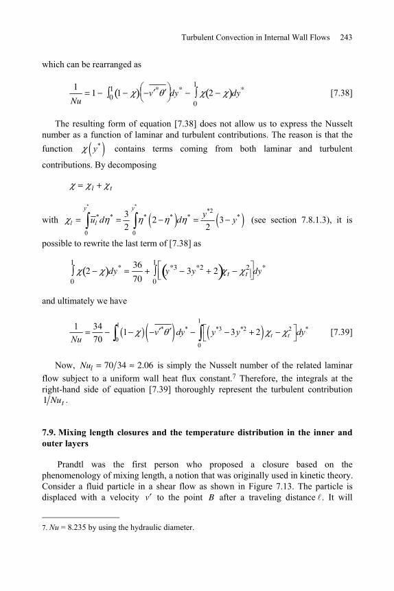
Turbulent Convection in Internal Wall Flows 243
which can be rearranged as
1
Nu1 10
1 v * dy* 2 dy*
0
1
[7.38]
The resulting form of equation [7.38] does not allow us to express the Nusselt number as a function of laminar and turbulent contributions. The reason is that the function *y contains terms coming from both laminar and turbulent
contributions. By decomposing
l t
with
* **2
* * * * * *
0 0
3 2 32 2
y y
l ly
u d d y (see section 7.8.1.3), it is
possible to rewrite the last term of [7.38] as
2 dy*
0
1 36
70y*3 3y*2 2 t t
2
0
1dy*
and ultimately we have
11 * * *3 *2 2 *
00
1 34 1 3 270 t tv dy y y dy
Nu [7.39]
Now, Nul 70 34 2.06 is simply the Nusselt number of the related laminar flow subject to a uniform wall heat flux constant.7 Therefore, the integrals at the right-hand side of equation [7.39] thoroughly represent the turbulent contribution 1 Nut .
7.9. Mixing length closures and the temperature distribution in the inner and outer layers
Prandtl was the first person who proposed a closure based on the phenomenology of mixing length, a notion that was originally used in kinetic theory. Consider a fluid particle in a shear flow as shown in Figure 7.13. The particle is displaced with a velocity v to the point B after a traveling distance . It will
7. Nu = 8.235 by using the hydraulic diameter.
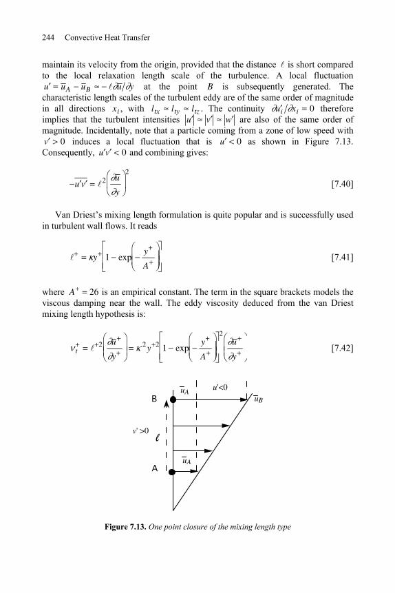
244 Convective Heat Transfer
maintain its velocity from the origin, provided that the distance is short compared to the local relaxation length scale of the turbulence. A local fluctuation u u A u B u y at the point B is subsequently generated. The characteristic length scales of the turbulent eddy are of the same order of magnitude in all directions xi , with ltx lty ltz . The continuity u i xi 0 therefore implies that the turbulent intensities u v w are also of the same order of magnitude. Incidentally, note that a particle coming from a zone of low speed with v 0 induces a local fluctuation that is u 0 as shown in Figure 7.13. Consequently, u v 0 and combining gives:
u v 2 u
y
2
[7.40]
Van Driest’s mixing length formulation is quite popular and is successfully used in turbulent wall flows. It reads
y 1 expy
A
[7.41]
where A 26 is an empirical constant. The term in the square brackets models the viscous damping near the wall. The eddy viscosity deduced from the van Driest mixing length hypothesis is:
t2 u
y2y 2 1 exp
y
A
2u
y
[7.42]
A
B
l
uB
uA
uAu'<0
v' >0
Figure 7.13. One point closure of the mixing length type
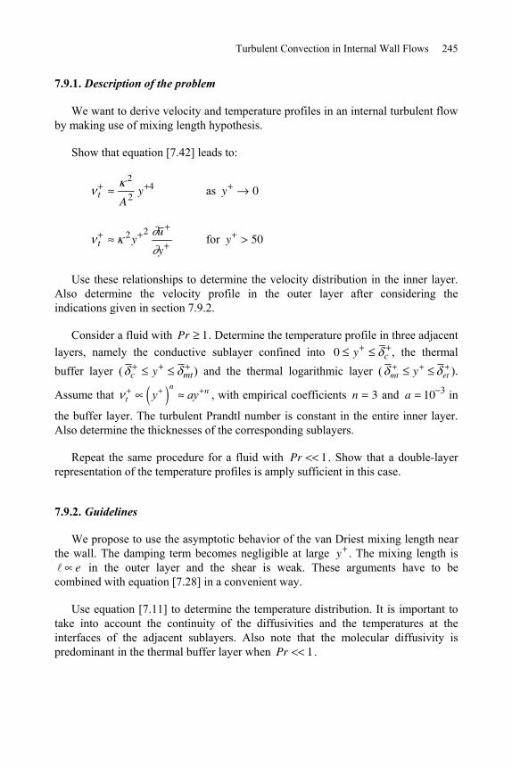
Turbulent Convection in Internal Wall Flows 245
7.9.1. Description of the problem
We want to derive velocity and temperature profiles in an internal turbulent flow by making use of mixing length hypothesis.
Show that equation [7.42] leads to:
t
2
A2y 4 as y 0
t2y
2 u
y for y 50
Use these relationships to determine the velocity distribution in the inner layer. Also determine the velocity profile in the outer layer after considering the indications given in section 7.9.2.
Consider a fluid with Pr 1. Determine the temperature profile in three adjacent layers, namely the conductive sublayer confined into 0 y c , the thermal buffer layer ( c y mt) and the thermal logarithmic layer ( mt y et ).
Assume that n n
t y ay , with empirical coefficients n 3 and a 10 3 in
the buffer layer. The turbulent Prandtl number is constant in the entire inner layer. Also determine the thicknesses of the corresponding sublayers.
Repeat the same procedure for a fluid with Pr 1 . Show that a double-layer representation of the temperature profiles is amply sufficient in this case.
7.9.2. Guidelines
We propose to use the asymptotic behavior of the van Driest mixing length near the wall. The damping term becomes negligible at large y . The mixing length is
e in the outer layer and the shear is weak. These arguments have to be combined with equation [7.28] in a convenient way.
Use equation [7.11] to determine the temperature distribution. It is important to take into account the continuity of the diffusivities and the temperatures at the interfaces of the adjacent sublayers. Also note that the molecular diffusivity is predominant in the thermal buffer layer when Pr 1 .
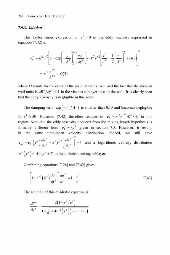
246 Convective Heat Transfer
7.9.3. Solution
The Taylor series expression at y 0 of the eddy viscosity expressed in equation [7.42] is
t2y 2 1 exp
y
A
2u
y
2y 2 y
A
1
2
y
A
2
O(3)
2
2 y 4
A 2O 5
where O stands for the order of the residual terms. We used the fact that the shear in wall units is u y 1 in the viscous sublayer next to the wall. It is clearly seen that the eddy viscosity is negligible in this zone.
The damping term exp y A is smaller than 0.13 and becomes negligible
for y 50 . Equation [7.42] therefore reduces to t2y
2u y in this
region. Note that the eddy viscosity deduced from the mixing length hypothesis is formally different from t y given in section 7.5. However, it results in the same time-mean velocity distribution. Indeed, we still have
22 2 1tot t
du duy y
dy dy and a logarithmic velocity distribution
lnu y A y B in the turbulent mixing sublayer.
Combining equations [7.28] and [7.42] gives:
21 1du du yy
dy dy e [7.43]
The solution of this quadratic equation is:
2
2 1
1 1 4 1
y edudy y y e
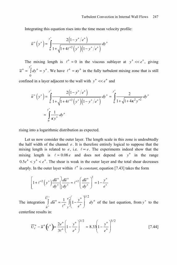
Turbulent Convection in Internal Wall Flows 247
Integrating this equation rises into the time mean velocity profile:
20
2 1
1 1 4 1
y y eu y dy
y y e
The mixing length is 0 in the viscous sublayer at y e , giving
u dy0
yy . We have y in the fully turbulent mixing zone that is still
confined in a layer adjacent to the wall with y e and
2 220 0
0
2 1 2
1 1 41 1 4 1
1
y y
y
y eu y dy dy
yy y e
dyy
rising into a logarithmic distribution as expected.
Let us now consider the outer layer. The length scale in this zone is undoubtedly the half width of the channel e . It is therefore entirely logical to suppose that the mixing length is related to e , i.e. e . The experiments indeed show that the mixing length is 0.08 e and does not depend on y in the range 0.5e y e . The shear is weak in the outer layer and the total shear decreases sharply. In the outer layer within is constant, equation [7.43] takes the form
22 21 1du du du yy
dy dy dy e
The integration du u
U c 11
y
ey
e1/ 2
dy of the last equation, from y to the
centerline results in:
U c u y2e
31
y
e
3 / 2
8.33 1y
e
3 / 2
[7.44]
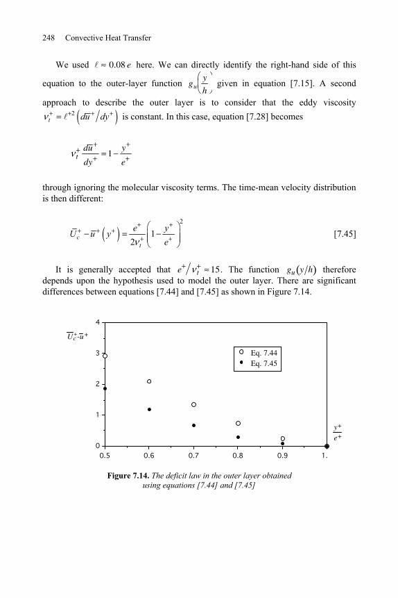
248 Convective Heat Transfer
We used 0.08 e here. We can directly identify the right-hand side of this
equation to the outer-layer function guy
h given in equation [7.15]. A second
approach to describe the outer layer is to consider that the eddy viscosity 2
t du dy is constant. In this case, equation [7.28] becomes
tdu
dy1
y
e
through ignoring the molecular viscosity terms. The time-mean velocity distribution is then different:
2
12c
t
e yU u ye
[7.45]
It is generally accepted that e t 15. The function gu y h therefore depends upon the hypothesis used to model the outer layer. There are significant differences between equations [7.44] and [7.45] as shown in Figure 7.14.
1.0.90.80.70.60.50
1
2
3
4
Eq. 7.44Eq. 7.45
Uc+-u+
y+
e+
Figure 7.14. The deficit law in the outer layer obtained using equations [7.44] and [7.45]
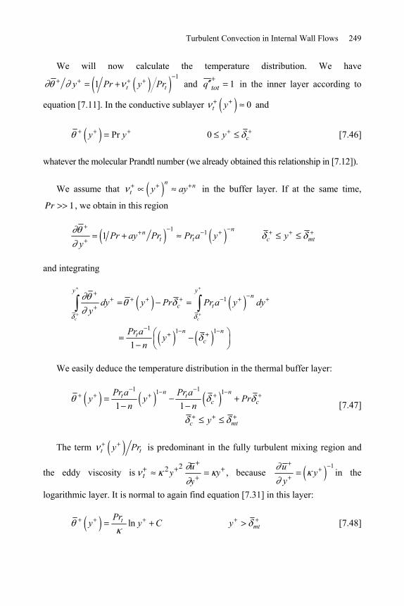
Turbulent Convection in Internal Wall Flows 249
We will now calculate the temperature distribution. We have 1
1 t ty Pr y Pr and q tot 1 in the inner layer according to
equation [7.11]. In the conductive sublayer 0t y and
Pr 0 cy y y
[7.46]
whatever the molecular Prandtl number (we already obtained this relationship in [7.12]).
We assume that n n
t y ay in the buffer layer. If at the same time,
Pr 1 , we obtain in this region
1 11nn
t t c mtPr ay Pr Pr a y yy
and integrating
1
1 1 1
1
c c
y yn
c t
n ntc
dy y Pr Pr a y dyy
Pr ay
n
We easily deduce the temperature distribution in the thermal buffer layer:
1 11 1
1 1n nt t
c c
c mt
Pr a Pr ay y Pr
n ny
[7.47]
The term t ty Pr is predominant in the fully turbulent mixing region and
the eddy viscosity is t2y
2 u
yy , because
1uy
yin the
logarithmic layer. It is normal to again find equation [7.31] in this layer:
lntmt
Pry y C y
[7.48]
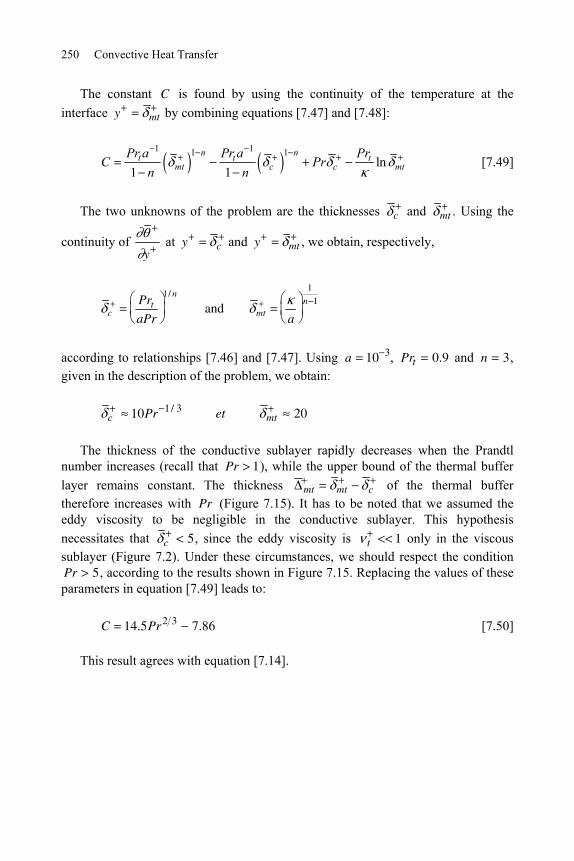
250 Convective Heat Transfer
The constant C is found by using the continuity of the temperature at the interface y mt by combining equations [7.47] and [7.48]:
1 11 1ln
1 1n nt t t
mt c c mtPr a Pr a Pr
C Prn n
[7.49]
The two unknowns of the problem are the thicknesses c and mt . Using the
continuity of y
at y c and y mt , we obtain, respectively,
cPrt
aPr
1/ n
and mt a
1
n 1
according to relationships [7.46] and [7.47]. Using a 10 3, Prt 0.9 and n 3, given in the description of the problem, we obtain:
c 10Pr 1 / 3 et mt 20
The thickness of the conductive sublayer rapidly decreases when the Prandtl number increases (recall that Pr 1), while the upper bound of the thermal buffer layer remains constant. The thickness mt mt c of the thermal buffer therefore increases with Pr (Figure 7.15). It has to be noted that we assumed the eddy viscosity to be negligible in the conductive sublayer. This hypothesis necessitates that c 5, since the eddy viscosity is t 1 only in the viscous sublayer (Figure 7.2). Under these circumstances, we should respect the condition Pr 5, according to the results shown in Figure 7.15. Replacing the values of these parameters in equation [7.49] leads to:
C 14.5Pr2 3 7.86 [7.50]
This result agrees with equation [7.14].
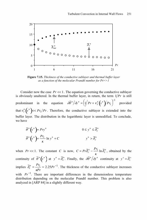
Turbulent Convection in Internal Wall Flows 251
211611610
5
10
15
20
Pr
mt + c
+
Figure 7.15. Thickness of the conductive sublayer and thermal buffer layer as a function of the molecular Prandtl number for Pr>>1
Consider now the case Pr 1 . The equation governing the conductive sublayer is obviously unaltered. In the thermal buffer layer, in return, the term 1 Pr is still
predominant in the equation y 1 Pr t y Prt
1 provided
that t y Prt Pr . Therefore, the conductive sublayer is extended into the
buffer layer. The distribution in the logarithmic layer is unmodified. To conclude, we have
y Pry 0 y c
yPrt ln y C y c
when Pr 1 . The constant C is now, C Pr cPrt ln c , obtained by the
continuity of y at y c . Finally, the y continuity at y c
implies cPrtPr
2.25Pr 1. The thickness of the conductive sublayer increases
with Pr 1. There are important differences in the dimensionless temperature distribution depending on the molecular Prandtl number. This problem is also analyzed in [ARP 84] in a slightly different way.
252 Convective Heat Transfer
7.10. Temperature distribution in the outer layer
7.10.1. Description of the problem
We have already introduced the temperature distribution in the outer layer in equation [7.16]. We will now show that more precise relationships can be obtained in the outer layer for the two classical boundary conditions that are constant wall temperature or uniform heat flux at the wall.
We seek to determine the temperature distribution in the outer layer for a fully developed turbulent channel flow with constant temperature at the wall by assuming that the turbulent flux terms are preponderant. Section 7.8.2 can be useful to this end.
Then solve the same problem when the wall flux is uniform. The departure point can be section 7.8.3.
7.10.2. Guidelines
The problem can be solved by using relationships [7.33] and [7.36]. It can further be shown that the temperature distribution in the outer layer depends on the boundary conditions. The eddy viscosity first increases linearly and subsequently reaches a constant that is typically t e 15 once y e 0.5 . The molecular viscosity can be ignored in this region. Similarly, the eddy diffusivity t t Prt is also constant in this zone providing that the turbulent Prandtl number does not vary with the wall normal distance y and that is the case for Pr 1 (Figure 7.4).
7.10.3. Solution
We will first consider the case with constant wall temperature. Equation [7.33], indicating that the total flux is constant, is written
q tot*
y*RePr v * Nu
[7.51]
It is recalled that the terms appearing in this equation are scaled by the outer variables introduced in section 7.8.2.3. The turbulent flux term RePr v * can be expressed as
RePr v * RePr t*
y*
Turbulent Convection in Internal Wall Flows 253
in the outer layer. Note that the eddy diffusivity t is non-dimensionalized by the outer scales, i.e. t
*t Ume . The dimensionless turbulent flux is larger than
y* which can consequently be ignored. The integration of [7.51], from y* being in this zone to the centerline ( y* 1), leads to:
c y*T c T y*
2Tw
Nu
RePr t*
1 y* Nu
RePr t*
1y
e
The term Re t* becomes:
Re t* Ume t
Ume t
Scaling with the flux temperature T q w results in an equation similar in form to [7.16]:
c y*T c T y*
T q w
2T w Nu
Pr t
1y
e [7.52]
It is clearly seen that the temperature varies linearly with y in the outer layer when the wall temperature is kept constant.
The temperature distribution is different in the outer layer in fully developed turbulent channel flow subject to uniform heat flux at the wall. Let us consider again the exact equation [7.36]
*
* * * * * **
0
1 1y
dy u d y v y
RePr dy
with T w x T x, y
T and T
q wcU m
(see section 7.8.3.2). The second term
on the right-hand side (molecular diffusion) is negligible in the outer layer and the eddy diffusivity is constant in the outer layer. Consequently
d
dy*y*
1 y*
t*
[7.53]
254 Convective Heat Transfer
resulting in
1* * *
**
1 1ct y
yy d
e
after integration. We use the heat flux temperature T q w q w cu to rewrite this
result in wall variables with, for instance, c c T T q w
1* * *
**
1* *
*
1 1
1
ct m y
t y
yy d
U e
e yd
e
[7.54]
since
t*U m
t
U me
U mu
t
e
It is clearly seen that the last relationship is totally different from equation [7.52] which corresponds to the constant wall temperature case. To simplify equation [7.54], let us assume that the velocity is constant and equal to the bulk velocity (which is indeed a very crude approximation). Then we have
*
* * * *
0
'u d , rising to:
2* 1
2ct
e yye
[7.55]
Note that there is a close similarity between equations [7.55] and [7.45] that correspond to the temperature and velocity distributions in the outer layer, respectively.
Turbulent Convection in Internal Wall Flows 255
7.11. Transport equations and reformulation of the logarithmic layer
The instantaneous local kinetic energy of the turbulence is defined
as K 1 2 u iu i , with the time mean K 1 2 u iu i 1 2 u 2 v 2 w 2 . The K
and T T dynamics play a key role both in the physical understanding of and modeling of the wall transfer mechanisms. The relations that govern these quantities are called turbulent transport equations. We propose to determine these equations. We will first determine the transport equation of the turbulent kinetic energy K and leave the reader to establish the relation governing T T . Some characteristics of the transport equations will subsequently allow us to obtain the logarithmic distributions in the fully turbulent mixing sublayers.
We consider a fully developed turbulent internal flow in a two-dimensional channel. The streamwise component of the Navier-Stokes equation reads for
u
tu u
u
xv
u
y
u
yw
u
z
1 p
x
1 p
x2 u u
with the time-mean average
01 p
x
2u
y2 yu v
The elimination of 1 p
x between these equations leads to the relation that
governs u x, y, z, t in time and space:
u
tu u
u
xv
u
y
u
yw
u
z
1 p
x2 u
yu v
[7.56]
Concurrently, v x, y, z, t and w x, y, z, t are governed by:
v
tu u
v
xv
v
yw
v
z
1 p
y2 v
w
tu u
w
xv
w
yw
w
z
1 p
z2 w
[7.57]
256 Convective Heat Transfer
We multiply equations [7.56] and [7.57] by u , v and w , and proceed to time-mean averaging. Adding the resulting equations leads to:
0 PK TK DK NK K
PK u v u
y
TKxi
u iK
DK
2 K
xk xk
N K1
xk
u k p
Ku ixk
u ixk
[7.58]
Each term of [7.58] has a clear physical meaning. The term PK represents the production. It regenerates the turbulence. The terms TK and NK correspond, respectively, to the turbulent transport and the pressure-velocity gradients redistribution. The molecular diffusion is denoted by DK . The turbulent dissipation
K regroups the correlations between the fluctuating velocity gradients. It plays a role as important as production does in the transport mechanisms.
Figure 7.16 shows the distributions of the turbulent kinetic energy transport budget terms in wall units. These results have been reported by [MAN 88] and obtained in a turbulent channel flow at Re 180 through direct numerical simulations. It is seen that production and dissipation dominate the kinetic energy transport.
The production reaches its maximum at y 12 where the streamwise turbulent intensity u u is also at its maximum (Figure 7.10). We note, in particular, that dissipation is in equilibrium with production at y 30 . This observation constitutes the basis of the present problem.
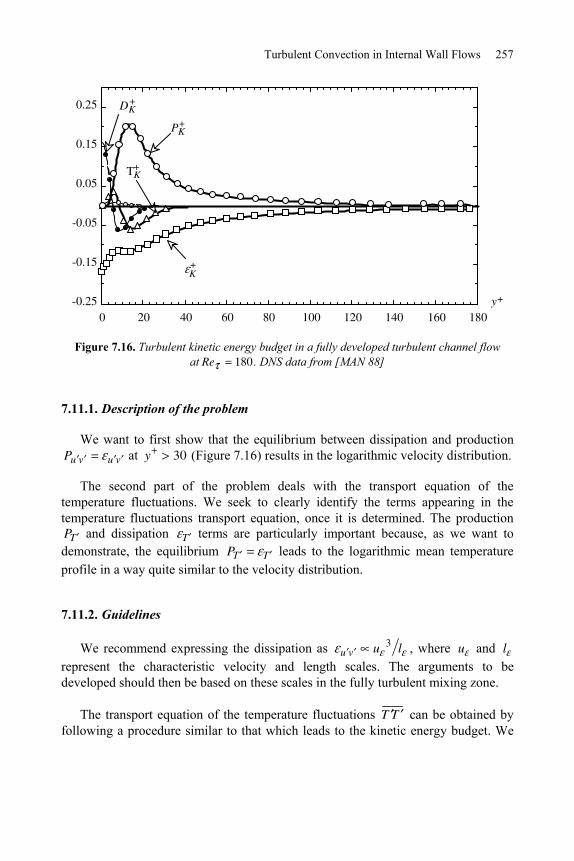
Turbulent Convection in Internal Wall Flows 257
180160140120100806040200-0.25
-0.15
-0.05
0.05
0.15
0.25 DK +
PK +
TK +
K +
y+
Figure 7.16. Turbulent kinetic energy budget in a fully developed turbulent channel flow at Re 180 . DNS data from [MAN 88]
7.11.1. Description of the problem
We want to first show that the equilibrium between dissipation and production Pu v u v at y 30 (Figure 7.16) results in the logarithmic velocity distribution.
The second part of the problem deals with the transport equation of the temperature fluctuations. We seek to clearly identify the terms appearing in the temperature fluctuations transport equation, once it is determined. The production PT and dissipation T terms are particularly important because, as we want to demonstrate, the equilibrium PT T leads to the logarithmic mean temperature profile in a way quite similar to the velocity distribution.
7.11.2. Guidelines
We recommend expressing the dissipation as u v u 3 l , where u and l represent the characteristic velocity and length scales. The arguments to be developed should then be based on these scales in the fully turbulent mixing zone.
The transport equation of the temperature fluctuations T T can be obtained by following a procedure similar to that which leads to the kinetic energy budget. We
258 Convective Heat Transfer
then propose to model the turbulent thermal dissipation term as T 'q T '
2
2c21
u T 'l T ',
where q T ' represents a typical flux scale related to the dissipation, together with the associated velocity u T' and length l T' scales. Once more, we have to be careful when we determine these scales in the fully turbulent region. Both u v and T' , for instance, should be independent of molecular viscosity and diffusivity in this zone.
7.11.3. Solution
Consider the production term PK u v u y of the turbulent kinetic energy budget [7.58]. One has u v u 2 in the constant shear zone. This region is fully turbulent; it is sufficiently far away from the wall in order that the molecular viscosity is negligible compared to the eddy viscosity, yet close enough to the wall so that the total shear does not vary appreciably. Thus any quantity should depend on in this region. Given that the dissipation can be put in the form u v u 3 l (by simple dimensional analysis), we only have to correctly determine the velocity and length scales, u and l . The choice for u is, naturally, u . The dissipation length scale has to be based on a local scale, such that l y y . The equality
PK K then implies u
y
u
y, or in other words the logarithmic u distribution.
Let us now determine the budget for the temperature fluctuations. The temperature field is governed in time and space by
2T T T T T TTu u v w T T
t x y z
with the Reynolds average
u T
x2T
v T
y
Taking the difference between these equations yields the following relationship governing the instantaneous T field:
2T T T TT T T v T
u u v w Tt x x y z y
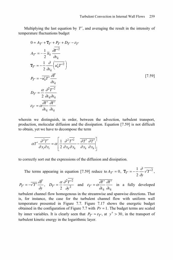
Turbulent Convection in Internal Wall Flows 259
Multiplying the last equation by T , and averaging the result in the intensity of temperature fluctuations budget
0 AT TT PT DT T
AT 1
2u k
T 2
xk
TT 1
2 xk
u kT 2
PT u kT T
xk
DT 2
2T 2
xk xk
T T
xk
T
xk
[7.59]
wherein we distinguish, in order, between the advection, turbulent transport, production, molecular diffusion and the dissipation. Equation [7.59] is not difficult to obtain, yet we have to decompose the term
2 2 21
2i i k k k k
T T T TT
x x x x x x
to correctly sort out the expressions of the diffusion and dissipation.
The terms appearing in equation [7.59] reduce to AT 0 , TT
1
2 yv T 2 ,
PT v T T
y, DT
2
2T 2
y2 and T
T
xk
T
xk
in a fully developed
turbulent channel flow homogenous in the streamwise and spanwise directions. That is, for instance, the case for the turbulent channel flow with uniform wall temperature presented in Figure 7.7. Figure 7.17 shows the energetic budget obtained in the configuration of Figure 7.7 with Pr 1. The budget terms are scaled by inner variables. It is clearly seen that PT T , at y 30 , in the transport of turbulent kinetic energy in the logarithmic layer.
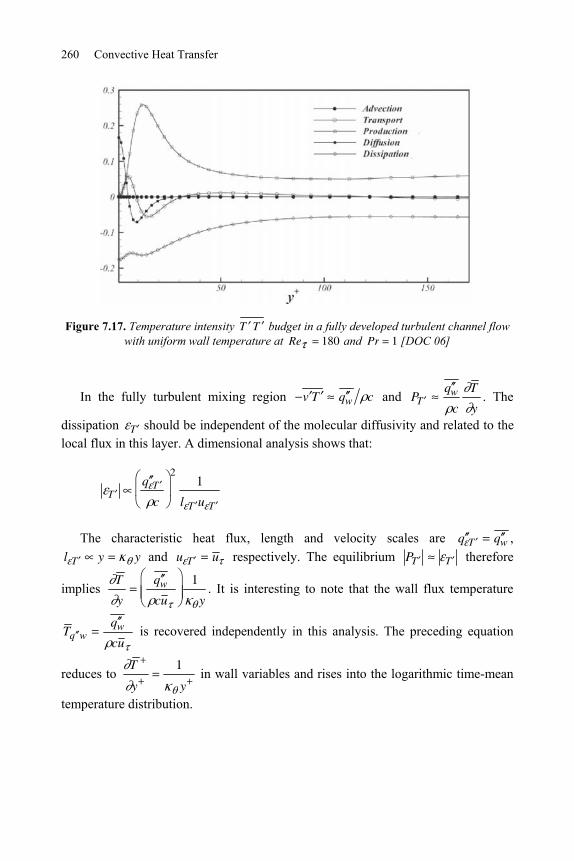
260 Convective Heat Transfer
Figure 7.17. Temperature intensity T T budget in a fully developed turbulent channel flow with uniform wall temperature at Re 180 and Pr 1 [DOC 06]
In the fully turbulent mixing region v T q w c and PT q w
c
T
y. The
dissipation T should be independent of the molecular diffusivity and related to the local flux in this layer. A dimensional analysis shows that:
T q T
c
21
l T u T
The characteristic heat flux, length and velocity scales are q T q w , l T y y and u T u respectively. The equilibrium PT T therefore
implies T
y
q wcu
1
y. It is interesting to note that the wall flux temperature
T q wq wcu
is recovered independently in this analysis. The preceding equation
reduces to T
y
1
y in wall variables and rises into the logarithmic time-mean
temperature distribution.
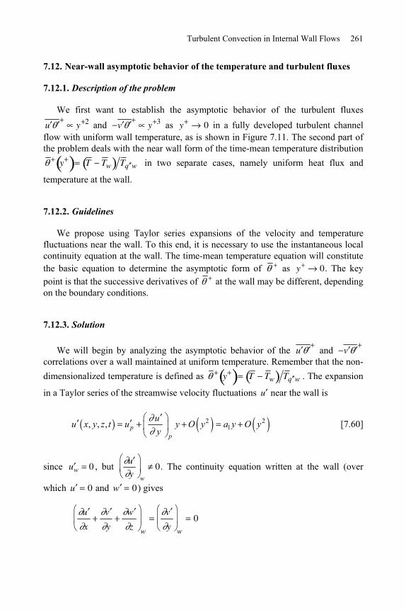
Turbulent Convection in Internal Wall Flows 261
7.12. Near-wall asymptotic behavior of the temperature and turbulent fluxes
7.12.1. Description of the problem
We first want to establish the asymptotic behavior of the turbulent fluxes u y 2 and v y 3 as y 0 in a fully developed turbulent channel flow with uniform wall temperature, as is shown in Figure 7.11. The second part of the problem deals with the near wall form of the time-mean temperature distribution
y T T w T q w in two separate cases, namely uniform heat flux and
temperature at the wall.
7.12.2. Guidelines
We propose using Taylor series expansions of the velocity and temperature fluctuations near the wall. To this end, it is necessary to use the instantaneous local continuity equation at the wall. The time-mean temperature equation will constitute the basic equation to determine the asymptotic form of as y 0. The key point is that the successive derivatives of at the wall may be different, depending on the boundary conditions.
7.12.3. Solution
We will begin by analyzing the asymptotic behavior of the u and v correlations over a wall maintained at uniform temperature. Remember that the non-dimensionalized temperature is defined as y T T w T q w . The expansion
in a Taylor series of the streamwise velocity fluctuations u near the wall is
2 21, , , p
p
uu x y z t u y O y a y O y
y [7.60]
since u w 0 , but u
y w
0. The continuity equation written at the wall (over
which u 0 and w 0) gives
u
x
v
y
w
z w
v
y w
0
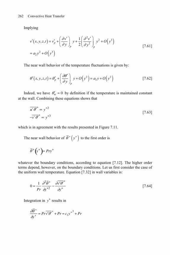
262 Convective Heat Transfer
Implying
22 3
2
2 32
1, , ,2p
p p
v vv x y z t v y y O y
y y
a y O y
[7.61]
The near wall behavior of the temperature fluctuations is given by:
2 23, , , p
p
x y z t y O y a y O yy
[7.62]
Indeed, we have w 0 by definition if the temperature is maintained constant at the wall. Combining these equations shows that
u' y 2
v' y 3
[7.63]
which is in agreement with the results presented in Figure 7.11.
The near wall behavior of y to the first order is
y Pry
whatever the boundary conditions, according to equation [7.12]. The higher order terms depend, however, on the boundary conditions. Let us first consider the case of the uniform wall temperature. Equation [7.32] in wall variables is:
01
Pr
2
y 2v
y [7.64]
Integration in y results in
yPrv Pr c1y
3Pr
Turbulent Convection in Internal Wall Flows 263
where we used the first order behavior of and the result [7.63] concerning v . Integrating the preceding equation again gives the asymptotic temperature behavior over a wall maintained at uniform temperature:
y Pry C1y 4 O y 5
[7.65]
Coupling between the convective heat transfer to the fluid and conduction to the solid is plausible in the uniform wall flux case. The temperature at the fluid-solid interface may vary in time resulting in:
x, y,z, t w y w
y O y2 a4 O y
Combining with the near wall behavior of the wall normal velocity fluctuations gives:
2 22v y c y
On the other hand, the time-mean temperature is now governed by:
u x
1Pr
2
y2
v
y [7.66]
Therefore, at the wall we have
2
y2
w
Prv
yu
xw
0
because v y 2 . The third derivative of the temperature at the wall is however different from zero, in contrast to the uniform wall temperature case. Indeed, deriving equation [7.66] with respect to y gives
u y x
w
u x y
w
0 ,
264 Convective Heat Transfer
since the heat flux at the wall is uniform, but the remaining terms are different from zero
3
y3
w
Pry
v
yu
xw
Pr 2c2u
y xw
0
Thus, the mean temperature varies as in
3 42Pry y C y O y
[7.67]
when y 0 over a uniform flux wall.
7.13. Asymmetric heating of a turbulent channel flow
7.13.1. Description of the problem
We consider a fully developed flow of water in a smooth turbulent regime through a channel with a rectangular cross-section (spacing 2e, span length Lz, e << Lz). The fluid is heated at uniform flux by one of the channel walls. The opposite wall is adiabatic (Figure 7.18). We propose to examine the influence of this asymmetric heating on the heat transfer law. The temperature difference between the two walls is more specifically investigated. We examine the thermally fully developed region where the mean fluid temperature may be written in the form:
T x, y T1 x T2 y
Notations, hypotheses and numerical data:
– zQ Q / L flow rate per transverse length unit 0.05 m3 s-1 m-1;
– Um bulk velocity;
– 2e channel width 5 cm; – x, y longitudinal and normal coordinates; – u friction velocity;
– q y heat flux in y direction;
– q w wall heat flux 5 104 W m-2; –Tw1
temperature of the heated wall;
–Tw2 temperature of the adiabatic wall;
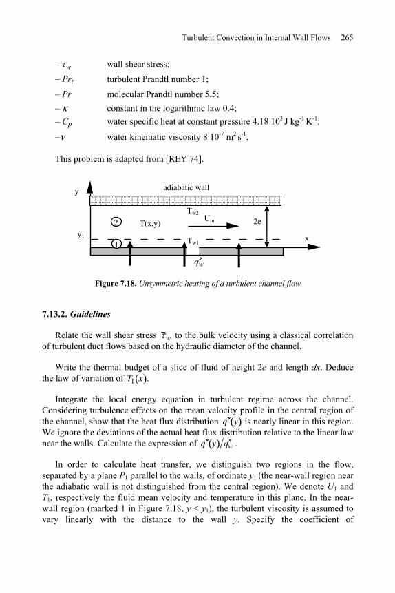
Turbulent Convection in Internal Wall Flows 265
– w wall shear stress; – Prt turbulent Prandtl number 1;
– Pr molecular Prandtl number 5.5; – constant in the logarithmic law 0.4; – Cp water specific heat at constant pressure 4.18 103 J kg-1 K-1;
– water kinematic viscosity 8 10-7 m2 s-1.
This problem is adapted from [REY 74].
Figure 7.18. Unsymmetric heating of a turbulent channel flow
7.13.2. Guidelines
Relate the wall shear stress w to the bulk velocity using a classical correlation of turbulent duct flows based on the hydraulic diameter of the channel.
Write the thermal budget of a slice of fluid of height 2e and length dx. Deduce the law of variation of T1 x .
Integrate the local energy equation in turbulent regime across the channel. Considering turbulence effects on the mean velocity profile in the central region of the channel, show that the heat flux distribution q y is nearly linear in this region. We ignore the deviations of the actual heat flux distribution relative to the linear law near the walls. Calculate the expression of q y q w .
In order to calculate heat transfer, we distinguish two regions in the flow, separated by a plane P1 parallel to the walls, of ordinate y1 (the near-wall region near the adiabatic wall is not distinguished from the central region). We denote U1 and T1, respectively the fluid mean velocity and temperature in this plane. In the near-wall region (marked 1 in Figure 7.18, y < y1), the turbulent viscosity is assumed to vary linearly with the distance to the wall y. Specify the coefficient of
x
y
T(x,y)Um
q w
y1
adiabatic wall
2e
1
2 Tw2
Tw1
266 Convective Heat Transfer
proportionality (it is suggested that the logarithmic law for the mean velocity be referred to). In the central region (marked 2 in Figure 7.18, y > y1), the turbulent viscosity is assumed to be constant and equal to tc. Experimental results show that u 2e/ tc = 26.
Calculate y1 2e by matching the turbulent viscosity at plane P1 between the regions 1 and 2. Calculate the mean velocity U1.
Relate the temperature difference Tw1T1 to q w by applying the Colburn
analogy in region 1, between the plane P1 and the heated wall.
Calculate the mean temperature distribution in region 2 by using the mean heat flux distribution. Calculate the wall temperature difference Tw1
Tw2 as a function of the parameters of the problem.
7.13.3. Solution
7.13.3.1. Wall shear stress
The bulk velocity is calculated by -11 m smU Q / 2e where zQ Q / L . The hydraulic diameter of the channel is Dh = 4e = 10 cm. The Reynolds number is calculated by Re UmDh 1 x 0.1 8 x10-7 = 1.25 105. The flow is therefore in turbulent regime. Assuming that roughness is sufficiently small for the flow to be in the smooth turbulent regime, the head loss coefficient is given by the Blasius law
0.316Re-1 4
from which the skin-friction coefficient is deduced as
C f 8 , with C f w Um2 .
The wall shear stress is obtained by:
w 0.039 Um2 Re-1 4 = 2.07 Pa.
The friction velocity is given by w u 2 . Hence, u = 0.045 m s-1.
Turbulent Convection in Internal Wall Flows 267
7.13.3.2. Thermal budget for a slice of fluid
We consider a slice of fluid of height 2e, length dx and span length Lz. Replacing T x by T1 x T2 y , the thermal budget yields:
Lzd
dxC pu y0
2e T1 x T2 y dy q wLz
Owing to effects of turbulence, the mean velocity profile is nearly flat in the central region of the channel and the high velocity gradient is concentrated in the very thin near-wall regions. Ignoring velocity variations in the above integral, the thermal balance becomes:
C pUm 2edT1
dxq w
[7.68]
Thus, the longitudinal temperature gradient is dT1 dx = "W pq / C Q. We find
dT1 dx = 0.24 °C m-1.
7.13.3.3. Heat flux distribution across the channel
For the present flow where the mean velocity field is one-dimensional, the local energy equation reduces to
C pu T
x
q y
y [7.69]
where q y is the total heat flux in the direction normal to the wall, namely the sum of the molecular ( k T y ) and the turbulent heat flux components ( C p v T ).
Integrating [7.69] across the channel, we obtain:
q y C pu T
xdy + Constant
In the central region, where the velocity profile is nearly flat, the mean velocity may be approximated by u Um and may be taken out the integral. The same holds
for T
x
T1
x. As a result, the heat flux distribution is nearly linear across the
central region of the channel.
268 Convective Heat Transfer
The heat flux must satisfy the boundary conditions:
q y 0 q w
q y 2e 0
We adopt the approximation that the linear distribution is also valid in the near-wall regions. The distribution of heat flux across the channel is then:
q y q w 1 y 2e [7.70]
It is worth noting that the unsymmetric heating induces different laws of distribution for the heat flux and the shear stress. In fact, the shear stress distribution is symmetric with respect to the plane of symmetry of the channel (y = e),
y w 1 y e (see section 7.8.1). This property is not satisfied by the heat flux. In particular, y e 0 whereas q y e q w 2 , according to [7.70]. It is therefore not possible to use calculation methods based on the statement that these two quantities have similar distributions across the channel as q y y q w w .
7.13.3.4. Determination of the boundary between the near-wall and the central regions
The logarithmic law is based on the turbulent viscosity model t u y ( = 0.4). Matching the laws for t at ordinate y1 in the near-wall and the central regions leads to:
t1 u y1 = tc with u 2e tc = 26.
y1
2e
1
26 = 0.096 [7.71]
which is rounded off to 0.1 because of the approximations of the model.
Thus, the boundary between the two regions is located at y1 5 mm, or in inner
variables, y1y1u
281.
The mean velocity U1 at the boundary between the two regions may be calculated by using the logarithmic law:
U11
0.4Lny1 5.5 = 19.6

Turbulent Convection in Internal Wall Flows 269
U1 = 0.88 m s-1.
As expected, this velocity is slightly smaller than Um .
7.13.3.5. Colburn analogy in the near-wall region
We apply the Colburn analogy in the near-wall region 1. This approach accounts for the molecular transfer, which plays an important role near the heated wall. The reference velocity is then U1 and the reference temperature scale is Tw1
T1.
St1C f1
Pr2 3
[7.72]
with C f1
w
U12
and St1q w
C pU1 Tw1T1
We find:
Tw1T1 Pr2 3 U1
C p
q w
w [7.73]
With the data of the problem, this relation gives Tw1T1 = 15.8°C.
7.13.3.6. Temperature distribution in the central region
Heat transfer is governed by turbulence in the central region so that the total heat flux is reduced to its turbulent component
q y C p v T = C p tT
y
where t is the thermal turbulent diffusivity.
Assuming Prt = 1, t is constant in the central region as is t . Accounting for [7.70], the mean temperature satisfies
T
y
q wC p t
1 y 2e
270 Convective Heat Transfer
which is integrated in
2 4"W
p 1
qT y y / e C
C
This temperature profile is matched to that of region 1 at y1:
T T1q wC p t
y y1y2 y1
2
4e
Assuming that this temperature distribution is valid up to the adiabatic wall, we obtain the temperature difference T1 Tw2
as:
T1 Tw2
q we
C p t
1y1
2e
2
[7.74]
The numerical data lead to T1 Tw2 = 2.8°C.
Combining [7.73] and [7.74], the wall temperature difference is finally obtained as:
Tw1Tw2
q w Pr2 3 U1
C p w
e
C p t
1y1
2e
2
[7.75]
The numerical value is Tw1Tw2
= 18.6°C.
We note the important temperature drop in region 1 that constitutes the main resistance to heat transfer and the weaker temperature drop in region 2 owing to the efficient turbulent mixing in the central region.
7.14. Natural convection in a vertical channel in turbulent regime
7.14.1. Description of the problem
We consider the cooling system of the fast neutron reactor core in a nuclear power plant in the situation when the coolant flow is accidentally lost. The system is simulated by a loop with mercury at moderate temperature as the coolant. In a loss-of-coolant accident, the fluid is maintained in motion by natural convection. The problem concerns the flow and heat transfer in a vertical channel (height L, spacing
Turbulent Convection in Internal Wall Flows 271
2e, span length Lz >> e), heated at uniform heat flux q along the lateral walls (Figure 7.19). The ratio L/e being much larger than 1, entrance effects are ignored so that the flow is assumed to be thermally and hydrodynamically fully developed through the whole channel height. We assume that the flow is in turbulent regime (this assumption will be checked at the end of the calculation). We denote T0 the temperature and 0 the density at the channel inlet. We propose calculating the flow rate through the channel and the difference between the wall and the fluid bulk temperature.
Geometrical data: e = 2 cm, L = 1 m. The surface roughness is assumed to be negligible.
Physical properties of mercury: – Density 0 = 13.6 103 kg m-3 – Kinematic viscosity = 10-7 m2 s-1 – Thermal conductivity k = 8.7 W m-1K-1 – Prandtl number Pr = 0.0249 – Specific heat at constant pressure C p = 140 J kg-1 K-1 – Coefficient of thermal expansion = 10-4 K-1
The channel is heated at uniform heat flux q = 103 W m-2.
7.14.2. Guidelines
The velocity and thermal fields are assumed to be two-dimensional. It is proposed that we first consider the momentum budget for the flow. The modified pressure is defined by
p* p 0gx
where x denotes the vertical abscissa, with the channel inlet being taken as the origin. We denote Tw x the wall temperature and y the total shear stress at any point in a channel cross-section.
Write the local Reynolds equation in a channel cross-section. Integrate this equation over the cross-section to obtain the global momentum budget for a slice of fluid of height dx.
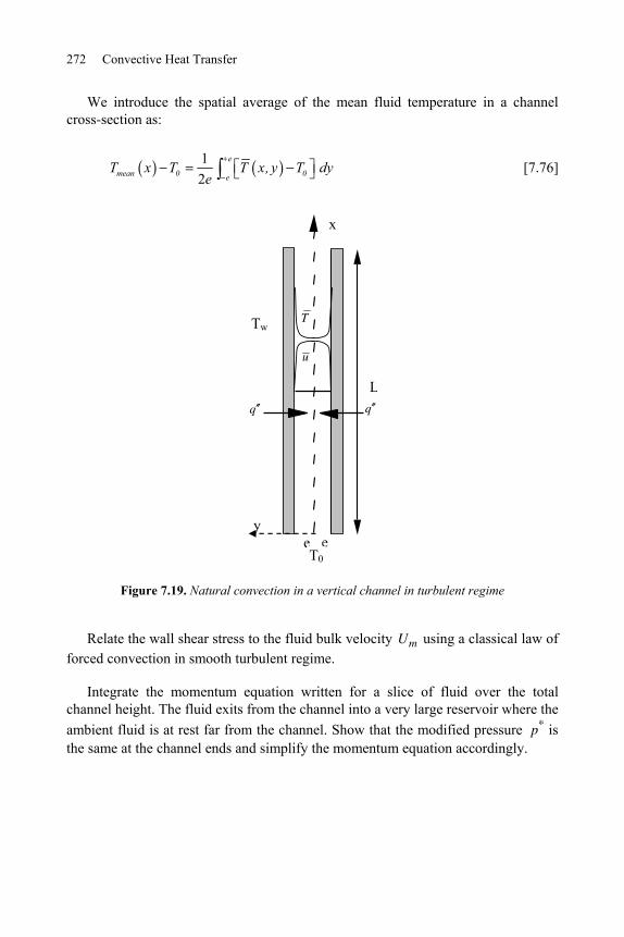
272 Convective Heat Transfer
We introduce the spatial average of the mean fluid temperature in a channel cross-section as:
12
e
mean 0 0eT x T T x, y T dy
e [7.76]
y
x
e e
Lq
Tw
T0
u
T
q
Figure 7.19. Natural convection in a vertical channel in turbulent regime
Relate the wall shear stress to the fluid bulk velocity Um using a classical law of forced convection in smooth turbulent regime.
Integrate the momentum equation written for a slice of fluid over the total channel height. The fluid exits from the channel into a very large reservoir where the ambient fluid is at rest far from the channel. Show that the modified pressure p* is the same at the channel ends and simplify the momentum equation accordingly.
Turbulent Convection in Internal Wall Flows 273
The mean velocity and temperature profiles are assumed to obey the classical power law with the exponent 1/7 as
u y1
Ua
Tw x T x, y1
Tw x Ta x1 7 with y1 e [7.77]
where Ua and Ta are, respectively, the velocity and temperature on the axis of symmetry of the channel, and y1 is the distance to a wall.
Show that the difference between the fluid bulk temperature Tm x and the spatially averaged temperature Tmean x is very weak in fully developed regime. These two quantities are not distinguished in the following discussion.
Starting from the energy budget written for a slice of fluid of height dx and width 2e, determine the temperature distribution Tm x along the channel when axial conduction is ignored. Calculate the expression of the buoyancy term in the momentum equation as a function of the parameters of the problem. Represent the momentum equation in the form ,*Re = f Gr Pr , where Re = UDh ( Dh
denotes the hydraulic diameter of the channel). Express Gr* as a function of the parameters of the problem.
Use a correlation of forced convection for metal liquid flows to calculate the heat-transfer coefficient h and the difference between the wall and the fluid bulk temperature.
Numerical application
Calculate: – the bulk velocity; check that the flow regime is turbulent; – the heat-transfer coefficient h and the difference between the wall and the fluid
bulk temperature; check that the Colburn analogy has poor accuracy in the present case; – the temperature difference between the channel inlet and outlet; – the friction velocity; – the viscous sublayer thickness; – the temperature fluctuation scale; – the temperature drop across the viscous sublayer.
Discuss the result.
274 Convective Heat Transfer
7.14.3. Solution
7.14.3.1. Momentum budget
In a fully developed regime, the mean longitudinal velocity is independent of x and the mean normal velocity is zero everywhere in the channel. As a result, the inertia term is zero in the Reynolds equation along x, which becomes
0p*
x0g T T0
y [7.78]
where T x, y is the mean temperature and y the total shear stress at a current point in the channel. Note that y does not depend on x since the flow is fully
developed. The Reynolds equation in normal direction gives p* y 0 , so that the mean pressure only depends on x.
We integrate equation [7.78] between the two channel walls:
*
0 00 2e
e
pe g T T dy e e
x [7.79]
Equation [7.79] results from equilibrium between the resultant of pressure forces, buoyancy forces and friction forces on the walls for a slice of fluid delimited by the channel walls (Figure 7.20). We introduce the spatial average of T x, y over a channel cross-section ([7.76]). Assuming that the mean velocity profile is symmetric with respect to the axis of symmetry of the channel ( e e ), we obtain:
0p*
xe 0g e Tmean T0 e
[7.80]
Let us remember that the wall shear stress is related to the mean velocity profile by e u y y e . This quantity is negative (Figure 7.19).
Equation [7.80] is finally integrated between the channel inlet and outlet. End effects are ignored; in other words, the regime is assumed to be fully developed over the whole channel length:
* *0 0
00 0
L
moyp p L e g e T x T dx e L
[7.81]
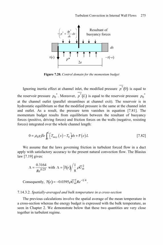
Turbulent Convection in Internal Wall Flows 275
p*
p* p*
xdx
ee
Resultant of buoyancy forces
2e
dx
Figure 7.20. Control domain for the momentum budget
Ignoring inertia effect at channel inlet, the modified pressure p* 0 is equal to
the reservoir pressure p0* . Moreover, p* L is equal to the reservoir pressure p0
* at the channel outlet (parallel streamlines at channel exit). The reservoir is in hydrostatic equilibrium so that the modified pressure is the same at the channel inlet and outlet. As a result, the pressure term vanishes in equation [7.81]. The momentum budget results from equilibrium between the resultant of buoyancy forces (positive, driving forces) and friction forces on the walls (negative, resisting forces) integrated over the whole channel length:
0 00
0L
moyg e T x T dx e L
[7.82]
We assume that the laws governing friction in turbulent forced flow in a duct apply with satisfactory accuracy to the present natural convection flow. The Blasius law [7.19] gives:
0.3164
Re0.25 with e
1
8U m
2
Consequently, e 0.0395 U m2Re 1 4 .
7.14.3.2. Spatially-averaged and bulk temperature in a cross-section
The previous calculations involve the spatial average of the mean temperature in a cross-section whereas the energy budget is expressed with the bulk temperature, as seen in Chapter 2. We demonstrate below that these two quantities are very close together in turbulent regime.
276 Convective Heat Transfer
The velocity and temperature profiles being symmetric, equation [7.76] may be restricted to a half-part of the channel cross-section. Moreover, the temperature may be conveniently referred to the wall temperature Tw , which is independent of y, instead of T0 , to calculate the integral. We assume that the half-part of the velocity and temperature profiles corresponding to 0 y1 e ( y1 e y ) is well described by [7.77]. The spatial average of the mean temperature in a cross-section is then obtained by:
Tw Tmean x1
eTw T x, y10
e dy1
Using [7.77], we find:
Tw Tmean Tw Ta1 7
01 d
7
8Tw Ta
The bulk velocity is calculated with the same procedure and the result is
U m7
8U a , where U a denotes the mean velocity on the channel axis.
According to its definition, the bulk temperature is calculated by:
Tw Tm1
U meu y1 Tw T x, y10
e dy1
Using [7.77] again, integration gives:
Tw Tm Tw TaU aU m
1 7 1 701 d
8
7
7
9Tw Ta
8
9Tw Ta
Finally:
Tw Tmean
Tw Tm
63
640.984
[7.83]
We conclude that the difference between the fluid bulk temperature Tm x and the spatially averaged temperature Tmean x is very weak and we replace Tmean x with Tm x in the following calculations.
Turbulent Convection in Internal Wall Flows 277
7.14.3.3. Energy budget
The energy budget for a slice of fluid of height dx and width 2e (Figure 7.20) yields
C pU m 2e dTm 2q dx
from which it follows that dTm
dx
q
C pU me
Thus, since the heat flux is uniform:
Tm xq
C pU mex T0
[7.84]
Hence, for these conditions of hydrodynamically fully developed regime and uniform wall heat flux heating, the energy budget gives a simple relation between the bulk temperature and the unknown bulk velocity.
7.14.3.4. Bulk velocity
The linear temperature distribution [7.84] is introduced into the integral of equation [7.82].
Tmean x T00L dx Tm x T00
L dxq
C pU me
L2
2
Equation [7.82], completed with Blasius law, becomes:
0 gq
C p
L 0.079 0U m3Re 1 4
The second term of the above equation may be expressed as a function of the Reynolds number only. The equation becomes:
0.079Re11 4 gq
0C p
LDh3
3
278 Convective Heat Transfer
Rearrangement of the right-hand side reveals the Grashof number associated with uniform heat flux heating:
Gr* g q k LDh3
2 [7.85]
The dimensionless bulk velocity is expressed by:
Re12.66Gr*
Pr
4 11
[7.86]
7.14.3.5. Heat-transfer coefficient
We use a correlation of forced convection for metal liquid flows [7.23] with the Reynolds number calculated above:
Nu 6.3 0.0167Re0.85Pr0.93 [7.87]
We deduce the heat-transfer coefficient h Nu k Dh and the temperature difference Tw Tm q h from the above equation. Note that Tw Tm is constant along the channel in a fully developed regime.
7.14.3.6. Numerical application
Hydraulic diameter: for a channel of high aspect ratio ( e Lz ), the hydraulic diameter is given by:
Dh4 x 2eLz
2 e Lz
4e = 0.08 m
Grashof number:
Gr* 9.81x1.82 x10-4 x12 x103 x 0.083
8.7 x 1.14 x10-7 29.7 x10¹⁰
Reynolds number [7.86]:
Re =9.7 x10¹⁰
0.079 x 0.0249
4 11
9.5 x10⁴
Turbulent Convection in Internal Wall Flows 279
This result shows that the flow is effectively in a turbulent regime.
Bulk velocity:
U m = 9.5 x104 x1.14 x10 7
0.08 = 0.134 m s-1
Flow rate per transverse length unit:
Q Lz = U m 2e = 0.135 x 0.04 = 5.4 x 10⁻³ m3 s-1 m-1
Nusselt number [7.87]:
Nu 6.3 0.0167 9.5 x10⁴ 0.850.02490.93 15.5
It is worth noting the low value of Nu which is due to the very small Prandtl number of a liquid metal. This result is, however, compensated for by the high value of thermal conductivity:
h 15.5 x 8.7 0.08 = 1680 W m-2K-1
Difference between the wall and bulk temperature in a channel cross-section:
Tw Tm 12 x103 1680 = 7.1 K
This difference is constant along the channel in the fully developed regime. Between the channel inlet and outlet, the fluid bulk temperature increase is calculated by [7.84]:
Tm x T012 x103
13.6 x103 x140 x 0.135 x 0.02 = 2.3 K
For better accuracy, axial conduction effects should be taken into account for this fluid at Pr << 1.

This page intentionally left blank
Chapter 8
Turbulent Convection in External Wall Flows
8.1. Introduction
This chapter deals with heat transfer in turbulent boundary layers. The main area of external turbulent flows is aerodynamics. This chapter is not self-contained, and several theories developed in the previous chapter will be directly applied to the local formulations that will be developed in this chapter.
8.2. Transition to turbulence in a flat plate boundary layer
The critical transition Reynolds number in a Blasius boundary layer is:
Rex,critu x
crit
3.5 105 to 106 [8.1]
The critical Reynolds number Rex,crit depends very much upon the perturbations present in the outer layer and may significantly increase if the perturbations u in the potential flow are particularly weak. We have
Re ,critu
crit
3000 to 5000 [8.2]
obtained by combining the laminar Blasius boundary layer thickness 5 x u with the preceding equation.
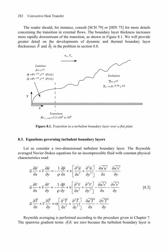
282 Convective Heat Transfer
The reader should, for instance, consult [SCH 79] or [HIN 75] for more details concerning the transition in external flows. The boundary layer thickness increases more rapidly downstream of the transition, as shown in Figure 8.1. We will provide greater detail on the developments of dynamic and thermal boundary layer thicknesses and T in the problem in section 8.8.
y
x
x1/2
T Pr -1/3 x1/2 (Pr 1)
T Pr -1/2 x1/2 (Pr 1)
u , T
x4/5
Laminar
Turbulent
T Pr -0.58 x 4/5
TransitionRe x , crit =3.5 105 to 106
Figure 8.1. Transition in a turbulent boundary layer over a flat plate
8.3. Equations governing turbulent boundary layers
Let us consider a two-dimensional turbulent boundary layer. The Reynolds averaged Navier-Stokes equations for an incompressible fluid with constant physical characteristics read:
2 2
2 21u u p u u u u u vu v
x y x x yx y
2 2
2 21v v p v v u v v vu v
x y y x yx y [8.3]
2 2
2 2T T T T u T v Tu vx y x yx y
Reynolds averaging is performed according to the procedure given in Chapter 7. The spanwise gradient terms z are zero because the turbulent boundary layer is
Turbulent Convection in External Wall Flows 283
two-dimensional (for instance, in the case of a boundary layer over a flat plate it is assumed that the plate is infinitely long in the spanwise direction). The last terms of this equation regroup the contributions of the turbulent heat flux. The boundary layer approximations that we will develop are based on peculiar characteristics of the order of magnitude of fluctuations u , v and w . The continuity requires:
u
x
v
y
w
z0
A turbulent structure that generates the fluctuating field is approximately isotropic1 which means that its characteristic length scales in all three directions are locally of the same order of magnitude lx ly lz l (in Figure 8.2, the symbol has to be interpreted as of the same order of magnitude and not approximately equal to). The continuity equation therefore implies u v w u . Noting by L the streamwise characteristic length of the boundary layer, the order of magnitudes of the Reynolds averaged terms become
u u
x
u 2
Lu v
y
u 2
and
u T
x
u T L
v T
y
u T
T
because L and T L . Here T stands for the order of magnitude of temperature fluctuations. The analysis of the other terms is entirely similar to that of laminar boundary layers, i.e.:
2u
x2
2u
y2
2T
x2
2T
y2
p
y
p
xp p x
1 dp
dxu
du
dx
1. Wall turbulence is anisotropic in the inner layer, but that does not modify the arguments advanced here, since the length scales of the turbulent wall eddies are still of the same order of magnitude in all directions (an order of magnitude means a factor of 10 or less).
284 Convective Heat Transfer
We finally establish the following turbulent boundary layer equations for the velocity and temperature fields:
u u
xv
u
yu
du
dx
2u
y2u v
y
u T
xv
T
y
2T
y2v T
y
[8.4]
8.4. Scales in a turbulent boundary layer
Scales governing the physics of turbulence and wall transfer are similar to those already introduced in Chapter 7, section 7.4. The inner scales are related to the local shear (friction) velocity and the molecular viscosity . The couple u x , x
constitutes the outer scales. The temperature scale in wall variables is still
T q w q w k ld q w cu x
where ld u x l x Pr is the characteristic diffusive length scale. The ensemble of these quantities depends on the streamwise location x . The non-dimensionalization that is necessary for closures has only a local meaning at a specified x . The underlying assumption is local equilibrium. The local equilibrium concept is delicate and it is beyond the context of this textbook. The interested reader may consult [TOW 76] as a starting point.
8.5. Velocity and temperature distributions
The eddy viscosity/diffusivity approach introduced in Chapter 7, section 7.5 is still valid in the context of turbulent boundary layers, provided that local inner scaling is used. The wall turbulence phenomenology near the wall is similar to internal turbulent flows under these conditions. Thus the velocity distribution in a turbulent boundary layer with zero pressure gradient (over a flat plate) is given by
u y y 5
u y1
ln y B 30 y2
U c u y guy
h 2y
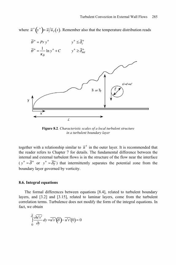
Turbulent Convection in External Wall Flows 285
where u y u u x . Remember also that the temperature distribution reads
Pr y y c
1ln y C y mt
Figure 8.2. Characteristic scales of a local turbulent structure in a turbulent boundary layer
together with a relationship similar to u in the outer layer. It is recommended that the reader refers to Chapter 7 for details. The fundamental difference between the internal and external turbulent flows is in the structure of the flow near the interface ( y or y T ) that intermittently separates the potential zone from the boundary layer governed by vorticity.
8.6. Integral equations
The formal differences between equations [8.4], related to turbulent boundary layers, and [3.2] and [3.15], related to laminar layers, come from the turbulent correlation terms. Turbulence does not modify the form of the integral equations. In fact, we obtain
u v
ydy
0u v u v 0 0
286 Convective Heat Transfer
and
v T
ydy
0
T
v T T v T 0 0
The immediate conclusion is that the integral equations of turbulent and laminar boundary layers are formally identical to
d u (x)dx
u (x)u (x)
2 u (x) *(x) C f (x)
u (x) d h2
dx2 h
2 du (x)dx
2Pr
h
c
already introduced in Chapter 3. The quantities appearing in the laminar integral equations have just been substituted by their Reynolds averaged values. Section 8.8 is an example showing how the integral equations can be applied to a turbulent boundary layer over a flat plate.
8.7. Analogies
Let us consider the local total shear and heat flux defined in Chapter 7:
tot t yu
y
q tot c t yT
y
The ratio of these quantities gives:
tot
q tot c
t y
t y
u
T [8.5]
The Reynolds analogy assumes that the ratio
t y
t yC
Turbulent Convection in External Wall Flows 287
is constant in the entire turbulent layer. This assumption is coupled with the hypothesis that tot w and q tot q w , which means that a particular accent is put on the fully turbulent mixing zone. Simple velocity and temperature profiles, such as
u y and T Tw y ,
are considered in a layer of thickness w , that includes the viscous and conductive sublayers. The profiles are assumed to be uniform in the turbulent core immediately adjacent ( y w ) and in which the velocity and the temperature are equal to their respective bulk values:
u Um1
u dy0
T Tm1
Umu T dy
0
The last equation is valid for Pr 1; the thermal boundary layer thickness T should be substituted in in the opposite case. These hypotheses simplify the integration of [8.5], leading to
w
q w c
t y
t y
Um
Tw Tm
[8.6]
that can be rearranged as
Stt y
t yC f [8.7]
where the Stanton number and the drag coefficient are respectively defined as
Sth
cUm
q wTw Tm cUm
, C fw
Um2
The Reynolds analogy goes through further simplifications by ignoring the molecular viscosity and diffusivity and assuming that the turbulent Prandtl number is approximately one
t y
t yt y
t yPrt y 1
288 Convective Heat Transfer
leading to the simple equation
St C f [8.8]
This relation ignores the role played by the viscous and conductive sublayers. Consequently, the Reynolds analogy has limited area of application. We know, for instance (from, for example, the Colburn correlation, see below), that the relationship between the Stanton number and the drag coefficient has to contain a dependence on the Prandtl number. That is found in the Prandtl-Taylor analogy that considers equation [8.5] in each sublayer separately. It can be expressed as
St C f1 Prt
1 12C f1/ 2 Pr
Prt1
[8.9]
and is valid for Pr 1. We establish this relationship in section 8.10.
We also have the following useful correlations:
– Colburn:
St C f Pr 2 / 3
[8.10]
– Kader and Yaglom:
StC f
2.12 ln 2Rex C f 12.5Pr 2 / 3 2.12 ln Pr 7.2
for 5x105 Rex 5x106
[8.11]
One of these correlations gives the heat exchange coefficient h once the drag coefficient is known. The drag coefficient can be found from either the classical Blasius relationship
C f 0.0296Rex1 5 [8.12]
or the von Karman law
1 C f a blog10 C f Rex [8.13]
with a = 2.4, b = 5.87.
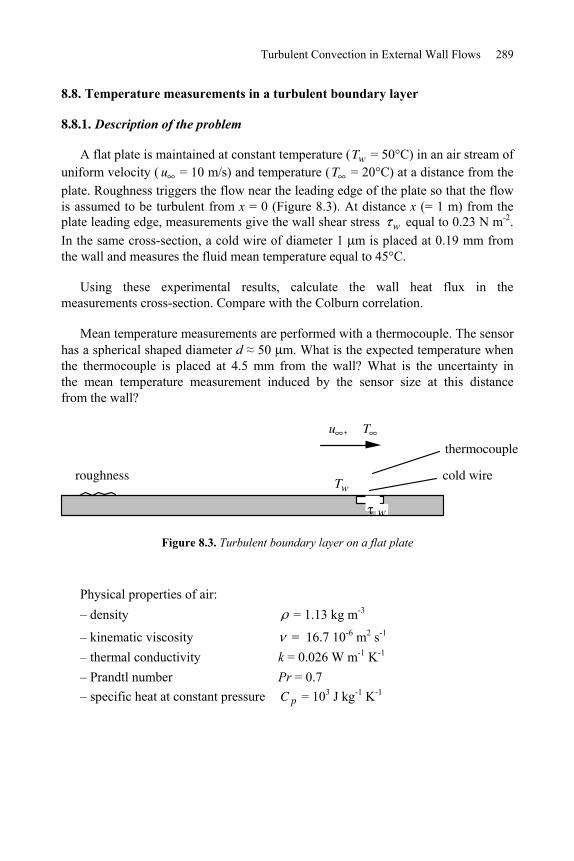
Turbulent Convection in External Wall Flows 289
8.8. Temperature measurements in a turbulent boundary layer
8.8.1. Description of the problem
A flat plate is maintained at constant temperature (Tw = 50°C) in an air stream of uniform velocity ( u = 10 m/s) and temperature (T = 20°C) at a distance from the plate. Roughness triggers the flow near the leading edge of the plate so that the flow is assumed to be turbulent from x = 0 (Figure 8.3). At distance x (= 1 m) from the plate leading edge, measurements give the wall shear stress w equal to 0.23 N m-2. In the same cross-section, a cold wire of diameter 1 m is placed at 0.19 mm from the wall and measures the fluid mean temperature equal to 45°C.
Using these experimental results, calculate the wall heat flux in the measurements cross-section. Compare with the Colburn correlation.
Mean temperature measurements are performed with a thermocouple. The sensor has a spherical shaped diameter d 50 m. What is the expected temperature when the thermocouple is placed at 4.5 mm from the wall? What is the uncertainty in the mean temperature measurement induced by the sensor size at this distance from the wall?
Figure 8.3. Turbulent boundary layer on a flat plate
Physical properties of air: – density = 1.13 kg m-3
– kinematic viscosity = 10-6 m2 s-1 – thermal conductivity k = 0.026 W m-1 K-1 – Prandtl number Pr = 0.7 – specific heat at constant pressure C p = 103 J kg-1 K-1
w
roughness
u , T
cold wire
thermocouple
Tw
290 Convective Heat Transfer
8.8.2. Solution
The friction velocity is calculated with the measured wall shear stress w :
w u 2
Hence, u 0.23 1.13 = 0.45 m s-1.
8.8.2.1. Measurements at 0.19 mm from the wall
The distance of the measurement point to the wall is expressed in wall units by:
yyu 0.19 x10 3 x 0.45
16.7 x10 6 = 5.1
This result shows that the measurement point is located in the viscous sublayer. It is therefore possible to calculate the wall heat flux by using the temperature gradient calculated over the distance of 0.19 mm between the measurement point and the wall:
q w kT
y 0
0.026 x50 45
0.19 x10 3 = 684 W m-2
The corresponding Stanton number is given by:
Stq w
C pu Tw T =
684
1.13 x103 x10 x 30 = 2.0 x 10⁻³
The skin-friction coefficient is calculated from the experimental wall shear-stress:
C fw
u 2 =
0.23
1.13 x102 = 2 x 10⁻³
The Colburn analogy gives
St C f Pr 2 / 3 = 2.53 x 10⁻³,
that is to say a difference of 26% relative to the direct measurement.
Turbulent Convection in External Wall Flows 291
8.8.2.2. Measurements at 4.5 mm from the wall
The distance of the measurement point from the wall is expressed in wall units by:
yyu 4.5 x10 3 x 0.45
16.7 x10 6 = 121
The measurement point is therefore located in the logarithmic layer. In wall units, the temperature is given by
1ln y C [8.14]
with 1 2.5 , C = 12.8 Pr0.68 – 7.3 for Prt 1 (equations [7.13] and [7.14]).
The logarithmic law gives:
1ln y C = 2.5 ln121 C
C 12.8 x 0.70.68 7.3 = 2.74
14.7
It is worth noting that combining equations [7.13] and [7.50] gives a result in close agreement with this value. In fact, with 1 0.9 x 2.5 2.25 , C 14.5Pr2 3 7.86 for Prt 0.9 , we find:
14.4
We use the definition of T w T
T q w
, with T q wq w
C pu
T q w684
1.13 x103 x 0.45 = 1.35°C
T w T 14.7 x1.35 = 20°C
292 Convective Heat Transfer
For a point located at 4.5 mm from the wall, the temperature is then expected to be:
T 30 °C
The thermocouple diameter is expressed in wall units as:
ddu 50 x10 6 x 0.45
16.7 x10 6 = 1.35.
The temperature variation over this distance is obtained by differentiating relation [8.14]:
1 y
y
1 d
y = 2.5
1.35
121= 2.8 x 10⁻²
Therefore, the temperature difference over a distance equal to the thermocouple diameter is:
T T q w = 1.35 x 2.8 x10 2 = 3.8 x10 2 °C
This variation is negligible relative to the measured temperature differences.
8.9. Integral formulation of boundary layers over an isothermal flat plate with zero pressure gradient
8.9.1. Description of the problem
We consider a thermal boundary layer over an isothermal flat plate. The free stream velocity is therefore uniform. We want to proceed through an integral analysis to determine the thermal and dynamic boundary layer thicknesses. The wall is maintained at uniform temperature Tw .
We will assume that local similarity solutions exist, with:
u x, y
ufu
y
x
Turbulent Convection in External Wall Flows 293
T x, y T
T w TfT
y
T x
Integral equations connected to turbulent boundary layers are similar in form to those governing laminar boundary layers. We recall that polynomial fu and fT profiles are generally chosen in the integral laminar boundary layer formulation (see Chapter 3). Polynomial distributions are, however, not convenient in turbulent boundary layers unless we take polynomials of very high degrees that are practically untreatable. The exact fu and fT profiles have to take into account the characteristics of different sublayers. We will therefore approach the problem in an approximate way by choosing power law distributions:
u x, y
u
y
x
1/ n
T x, y T
T w T1
y
T x
1/ n
Experiments show that these distributions are partially acceptable in the log and external sublayers (constituting of 80% of the total flow field) if we take n 7 , but they are obviously not valid in the internal layer. In fact, the shear and flux deduced from these relations become indefinite at the wall. We will address this drawback by assuming that the drag coefficient is given by the Blasius law:
C f xu
u
2
C1Re m C1u
m
The empirical coefficients appearing in this relationship are C1 0.0225 and m 0.25 . The aim is to determine x and T x . We also assume that the thermal and dynamic boundary layers start at the same point x 0. This problem is somewhat classical. It is treated in more or less different ways in several textbooks such as [SCH 79] or [ARP 84].
8.9.2. Guidelines
We have to use the integral equations dealing with velocity and temperature fields developing over a flat plate. These equations have to be modified to sort out the drag coefficient and the Stanton number. It will be necessary at this point to use
294 Convective Heat Transfer
an analogy between the wall heat flux and shear stress. We recommend the Colburn analogy, St x C f x Pr 2 / 3 . It is also assumed that the ratio between the thermal and dynamic boundary layer thicknesses T x x is a constant depending on the molecular Prandtl number.
8.9.3. Solution
The integral streamwise momentum and energy equations in a turbulent boundary layer are similar in form to those governing a laminar boundary layer. The integral momentum equation is:
d
dxu u u dy w
0
x
[8.15]
The time-mean temperature distribution is governed by:
d
dxC pu T T dy q w
0
T x
[8.16]
Dividing the two sides of equation [8.15] by u 2 (which does not depend on x ), using the definition of the skin-friction velocity w u 2 and of the drag
coefficient C f x u u2 leads to
u
u1
u
ud
0
1 d
dxC f x [8.17]
where we introduced the variable y x and assumed a similarity form u u fu . We will use the algebraic mean velocity profile fu
1/ n . Thus the integral appearing in the preceding equation is calculated as:
u
u1
u
ud
0
11/ n 1 1/ n d
0
1n
n 1 n 2
Turbulent Convection in External Wall Flows 295
Using the drag coefficient given by the Blasius law, and rearranging equation [8.17] gives:
d
dx
n 1 n 2
nC1
um
This equation now has to be integrated from the leading edge of the plate to some streamwise x position. The result is:
x
m 1 n 1 n 2
nC1
1m 1 u x
m
1 m
m 1 n 1 n 2
nC1
1m 1
Rex
m
1 m
[8.18]
The first conclusion that can be drawn from this relationship is that the turbulent boundary layer thickness varies like x1/ m 1 x 4 / 5 ( m 0.25), significantly more rapidly than the laminar boundary layer for which x1/ 2 (Chapter 3). Using the empirical coefficients m 0.25 , n 7 and C1 0.0225 in [8.18], it is further concluded that:
x0.37Rex
1/ 5 [8.19]
Integral equation [8.16] can be rearranged to give
d
dx
u
u
T T
Tw Tdy
q wC pu Tw T0
T x
[8.20]
because the wall temperature is uniform, the physical fluid characteristics are uniform and u does not depend upon x . We note the presence of the Stanton number at the right-hand side of this equation:
St xh x
c pu
q w x
cpu Tw T
296 Convective Heat Transfer
We further opt for the following self-similar distributions:
u
ufu
y
xand
T T
T w TfT
y
T x [8.21]
We will now assume that the ratio of the thermal to dynamic boundary layer thicknesses is independent of the streamwise position x and is a function of the molecular Prandtl number only with T x x Pr . Defining the new integration variable by y T x , using the empirical Colburn relation and combining with the Blasius law, we obtain:
St C f x Pr 2 / 3 C1Re m Pr 2 / 3
Thus, equation [8.20] now takes the form
fu fT d0
1 d T
dxC1Re m Pr 2 / 3 C1
u mm
Tm Pr 2 / 3
where the definition of has been used to eliminate . We will use simple similarity distributions
fu1/ n and fT 1 1/ n
resulting in
fu fT d0
1 d T
dx1/ n n
n 1 n 2d T
dx
Combining and integrating leads to:
T
x
m 1 n 1 n 2
nC1Pr 2 / 3
m1n
1m 1
Rex
m
1 m [8.22]
Turbulent Convection in External Wall Flows 297
The conclusion is that T x Rex
m
1 m Rex1/ 5 , exactly as for the boundary
layer thickness x . Dividing equation [8.22] by [8.18] and rearranging enables us to reach a relationship for the ratio of the boundary layer thicknesses, namely:
T x
xPr
2n
3(n 1) [8.23]
An equation that can be used in practical situations dealing with dimensionless thermal boundary layer thickness is finally obtained by using the empirical coefficients m 0.25 , n 7 and C1 0.0225 :
T
x0.37 Pr 0.58 Rex
1/ 5 [8.24]
8.10. Prandtl-Taylor analogy
8.10.1. Description of the problem
We discussed the Reynolds analogy in section 8.7. This is a crude approximation since it does not take into account the effect of the wall layer in which the turbulent viscosity and diffusivity are negligible compared to their molecular analogs.
The Prandtl-Taylor analogy divides the whole layer into two parts. The molecular viscosity and diffusivity are predominant in the wall layer of thickness
w . This layer extends to typically w 13 in inner variables. The turbulent bulk zone constitutes the adjacent sublayer in which t and t govern the flow and heat transfer.
To simplify the formulation of the problem, it will be assumed that both the mean velocity and the temperature are constant and equal to their consecutive bulk values in the fully developed turbulent sublayer as shown in Figure 8.4.
The solution requires a procedure similar to that conducted in section 8.7, but here we have to take into account the supplementary effect of the wall layer.
8.10.2. Guidelines
It is recommended that equation [8.5] is used as the departure point. This equation has to be integrated in the wall layer and subsequently the turbulent bulk
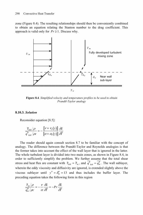
298 Convective Heat Transfer
zone (Figure 8.4). The resulting relationships should then be conveniently combined to obtain an equation relating the Stanton number to the drag coefficient. This approach is valid only for Pr 1. Discuss why.
U m
T m
Fully developed turbulent mixing zone
Near wall sub-layer
u w w
T w
T w
Figure 8.4. Simplified velocity and temperature profiles to be used to obtain Prandtl-Taylor analogy
8.10.3. Solution
Reconsider equation [8.5]:
tot
q tot c
t y
t y
u
T
The reader should again consult section 8.7 to be familiar with the concept of analogy. The difference between the Prandtl-Taylor and Reynolds analogies is that the former takes into account the effect of the wall layer that is ignored in the latter. The whole turbulent layer is divided into two main zones, as shown in Figure 8.4, in order to sufficiently simplify the problem. We further assume that the total shear stress and heat flux are constant with tot w , and q tot q w . The wall sublayer, wherein the eddy viscosity and diffusivity are ignored, is extended slightly above the viscous sublayer until y w 13 and thus includes the buffer layer. The preceding equation takes the following form in this region
w
q w c
u
T Pr
u
T
Turbulent Convection in External Wall Flows 299
whose integral is
c w
q wPr
u p
Tw T w
[8.25]
where w stands for the wall sublayer thickness. The molecular viscosity and diffusivity are negligible in the fully turbulent core. We further assume that the turbulent Prandtl number is constant
t y
t yPrt Ct
with
w
q w ct y
t y
u
T Prt
u
T
Integrating this equation from y p to y leads to:
c w
q wPrt
Um u w
T w
Tm
[8.26]
Eliminating T w
between equations [8.25] and [8.26] results in
T w
Tw Tm
1
where Prt Um u
w
u wPr
Substituting this expression into equation [8.26] gives
Tw Tmq w
c w
Prt Um u w
u wPr
UmPrt q wc w
1u
w
Um
Pr
Prt1
that may be rearranged to give
300 Convective Heat Transfer
St1 Prt
1u
w
Um
Pr Prt 1C f [8.27]
This relationship is known as the Prandtl-Taylor analogy. Remember that the Stanton number and the drag coefficient are respectively defined by:
Stq w
Tw Tm cUm
, C fw
Um2
The term under bracket at the right-hand side of equation [8.27] is the weighting factor of the drag coefficient. It represents the Prandtl-Taylor correction of the Reynolds analogy (equation [8.8]). The present approach is valid only for Pr 1. Indeed, in the opposite case of Pr 1 , the conductive sublayer may be considerably thicker than the viscous sublayer, which is contradictory to ignoring the molecular diffusivity at y w . For Pr 1 the conductive sublayer thickness decreases with Pr as c Pr 1/ 3 (see section 7.9). Ignoring the eddy diffusivity in the wall layer y w is therefore incorrect, in particular when Pr 1 , but that is the price to pay for having a simple approach.
We further have:
u w
Um
u w
Um
w
UmwC f
1/ 2 12C f1/ 2
We finally recover the form of the Prandtl-Taylor analogy as given by equation [8.9], namely:
St C f1 Prt
1 12C f1/ 2 Pr
Prt1
Note that St C f f Re,Pr,Prt , because the drag coefficient depends upon the Reynolds number.
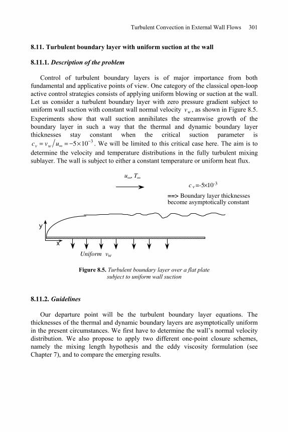
Turbulent Convection in External Wall Flows 301
8.11. Turbulent boundary layer with uniform suction at the wall
8.11.1. Description of the problem
Control of turbulent boundary layers is of major importance from both fundamental and applicative points of view. One category of the classical open-loop active control strategies consists of applying uniform blowing or suction at the wall. Let us consider a turbulent boundary layer with zero pressure gradient subject to uniform wall suction with constant wall normal velocity vw , as shown in Figure 8.5. Experiments show that wall suction annihilates the streamwise growth of the boundary layer in such a way that the thermal and dynamic boundary layer thicknesses stay constant when the critical suction parameter is cv vw u 5 10 3 . We will be limited to this critical case here. The aim is to determine the velocity and temperature distributions in the fully turbulent mixing sublayer. The wall is subject to either a constant temperature or uniform heat flux.
y
x
u , T
c v =-5 10-3
Uniform
==> Boundary layer thicknesses become asymptotically constant
vw
Figure 8.5. Turbulent boundary layer over a flat plate subject to uniform wall suction
8.11.2. Guidelines
Our departure point will be the turbulent boundary layer equations. The thicknesses of the thermal and dynamic boundary layers are asymptotically uniform in the present circumstances. We first have to determine the wall’s normal velocity distribution. We also propose to apply two different one-point closure schemes, namely the mixing length hypothesis and the eddy viscosity formulation (see Chapter 7), and to compare the emerging results.
302 Convective Heat Transfer
8.11.3. Solution
Recall the turbulent boundary layer equation:
u u
xv
u
y y
u
yu v
The boundary layer thickness no longer varies with x and therefore u x 0 in the so-called asymptotically fully developed zone. The continuity
equation leads to:
u
x
v
y
v
y0
Thus, we conclude that the wall’s normal velocity distribution is v vw 0 , since v does not depend upon x and is consequently constant in the entire layer. The boundary layer equation takes the form
vwdu
dy
d
dy
du
dyu v
that can be integrated from the wall ( y 0) to a point y in the boundary layer
vwdu
dy0
ydy
y
du
dyu v dy
0
y
giving
vwu ydu
dyu v
0
ydu
dyy u v y w [8.28]
because u v 0 at the wall and, by definition, u y y 0 w . We seek out
the velocity and temperature distributions in the fully turbulent region. We can consequently ignore the molecular viscous stress with respect to the Reynolds shear stress and rewrite equation [8.28] in wall units and u :
1 vwu u v [8.29]
Turbulent Convection in External Wall Flows 303
The final result will obviously depend upon the closure scheme that is used for u v . We have
u v 2y 2 du
dy
2
if we opt for the Prandtl mixing length hypothesis (see section 7.9). Therefore
1 vwu 1/ 2
ydu
dy [8.30]
which clearly shows that u is a function of y and vw . The preceding equation takes the following form by the transformation of the integration variable vwu
d
1 1 2vw
1 dy
y
whose integral is
2 1 1/ 2 C vw ln y C vp
Now, 0 when vw 0 and therefore the integration constant is C 2 . We consequently have the solution
2
vw
1 vwu 1/ 2
11
ln y C vw [8.31]
taking the explicit form
u 1
ln y C vw1
4vw
1ln y C vw
2
[8.32]
The term 1 4 vw 1 ln y C vw
2 decreases the mean velocity with respect to
the logarithmic distribution in the standard turbulent boundary layer because vw 0 . The classical logarithmic distribution should be recovered from equation [8.31] when vw 0 . In fact, a Taylor series expansion to the first order gives
304 Convective Heat Transfer
1 vwu 1/ 2
1 1 2 vwu for small vwu , and we find u 1 ln y C when
vw 0 .
A similar procedure enables us to determine the temperature field. The equation governing the temperature in the asymptotically developed thermal boundary layer wherein d T dx 0 is:
vwdT
dy
d
dy
dT
dyv T
The integration of this equation from the wall to some y position in the thermal boundary layer gives rise to:
vw T y T wq w
c
dT
dyv T
This relationship is local. We have to consider local values of q w x and T w x in the boundary conditions dealing with uniform wall temperature and heat flux respectively. Scaling the temperature by the wall variables T w T T q w and
ignoring the molecular heat flux dT dy compared to v T in the fully turbulent mixing zone, we obtain a relationship analog to equation [8.29], namely:
1 vw v T [8.33]
The integration of this equation combined with the closure2 v T t Prt y and t y , gives rise to:
1
vw
ln 1 vwPrt ln y C vw
1ln y C vw [8.34]
The asymptotic form of this distribution for vw 0 is the classical logarithmic
profile since ln 1 vw vw for small vw . The assumptions we made to
obtain equation [8.34] are: – the turbulent Prandtl number is constant;
2. varies in the opposite direction to T .
Turbulent Convection in External Wall Flows 305
– the logarithmic part of the thermal boundary layer merges into the logarithmic velocity sublayer justifying the use of t y in the eddy diffusivity formulation. Equation [8.34] can be modified to:
1
vw
exp vwC yvw 1
vw
[8.35]
The coefficient C depends on C C Pr, Prt , vw . The difference between
distributions [8.31] and [8.34] comes from the fact that we used a Prandtl mixing length closure for the mean velocity and an eddy diffusivity approach for the temperature. The reader can easily verify that using
u v tdu
dyy
du
dy
results in
u 1
vw
exp vwC yvw 1
vw
[8.36]
which is qualitatively equivalent to [8.35].
The constants C and C appearing in the velocity and temperature profiles expressions are functions of the wall suction velocity, and they can consequently be adjusted to collapse the results inferred from the models and the experiments. We show in Figure 8.6 the distributions given by equations [8.32] and [8.35] with Prt 1, 0.4 and C C 5. We took vw 0,1; in wall units that roughly corresponds to cv vw u 5 x10 3 rising into asymptotically constant boundary layer thicknesses sufficiently far away from the leading edge. The profiles are compared to the classical logarithmic distribution of the canonical turbulent boundary layer. We notice that suction flattens the velocity and temperature distributions and considerably reduces them compared to the standard law. The eddy viscosity model underestimates u and/or with respect to the Prandtl mixing length closure.
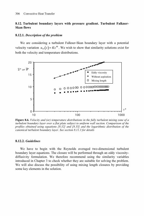
306 Convective Heat Transfer
8.12. Turbulent boundary layers with pressure gradient. Turbulent Falkner-Skan flows
8.12.1. Description of the problem
We are considering a turbulent Falkner-Skan boundary layer with a potential velocity variation u x Kxm . We wish to show that similarity solutions exist for both the velocity and temperature distributions.
1000100100
5
10
15
20
Eddy viscosity
Without aspiration
Mixing length
y+
u+ or +
Figure 8.6. Velocity and (or) temperature distributions in the fully turbulent mixing zone of a turbulent boundary layer over a flat plate subject to uniform wall suction. Comparison of the profiles obtained using equations [8.32] and [8.35] and the logarithmic distribution of the canonical turbulent boundary layer. See section 8.11.3 for details
8.12.2. Guidelines
We have to begin with the Reynolds averaged two-dimensional turbulent boundary layer equations. The closure will be performed through an eddy viscosity-diffusivity formulation. We therefore recommend using the similarity variables introduced in Chapter 3 to check whether they are suitable for solving the problem. We will also discuss the possibility of using mixing length closures by providing some key elements in the solution.
Turbulent Convection in External Wall Flows 307
8.12.3. Solution
Let us reconsider the Reynolds averaged equations [8.4] and combine them with the eddy viscosity-diffusivity closure:
u v t yu
y
v T t y
Prt y
T
y
The boundary layer equations of the problem are:
u
x
v
y0
u u
xv
u
yu
du
dx y1 t
u
y
u T
xv
T
y y
1Pr
t
Prt
T
y
[8.37]
The potential velocity is u x Kxm in the Falkner-Skan flows. They have already been analyzed in Chapter 3 in laminar boundary layers. Equations [8.37] differ in form from their laminar counterparts due to the presence of eddy viscosity-diffusivity terms and the turbulent Prandtl number. The supplementary terms with respect to the laminar boundary layer are:
y tu
y
yt
Prt
T
y [8.38]
It is therefore sufficient to duplicate the similarity analysis conducted in Chapter 3 by adding supplementary terms [8.38] to the laminar dynamic and thermal boundary layer equations. The similarity variable is still:
yu
x
1/ 2
308 Convective Heat Transfer
The velocity distribution is of the form:
u
u xF
We remember that a wall temperature variation of the form Tw T Hxn is necessary to ensure similarity solutions of the temperature field. The dimensionless temperature is defined as
T x, y T
Tw x T
in the same way as in Chapter 3. This representation is not appropriate in the case of specified heat flux at the wall q w x as in that caseTw x is unknown. The temperature scale related to q w x is deduced from dimensional analysis as
2/1xw Rekxxq where Rex u x . Therefore, the dimensionless temperature for
a specified wall heat flux is:
T x, y T
q w x x k Rex1/ 2
The condition for similarity is reduced to q w x x k Rex1/ 2 H xn in this case as
in laminar Falkner-Skan flows.
Equation [8.38] is transformed into:
yt
u
yt F
u2
x
yt
Prt
T
yTw x T t
Prt
u
xTw x specified
yt
Prt
T
yt
Prt
q w x
kxRex
1/ 2 q w x specified
[8.39]
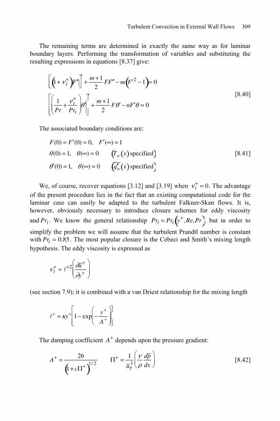
Turbulent Convection in External Wall Flows 309
The remaining terms are determined in exactly the same way as for laminar boundary layers. Performing the transformation of variables and substituting the resulting expressions in equations [8.37] give:
1 t F m 1
2FF m F 2 1 0
1Pr
t
Prt
m 12
F nF 0
[8.40]
The associated boundary conditions are:
F (0) F (0) 0, F ( ) 1
(0) 1, ( ) 0 Tw x specified
(0) 1, ( ) 0 q w x specified
[8.41]
We, of course, recover equations [3.12] and [3.19] when t 0. The advantage of the present procedure lies in the fact that an existing computational code for the laminar case can easily be adapted to the turbulent Falkner-Skan flows. It is, however, obviously necessary to introduce closure schemes for eddy viscosity and Prt . We know the general relationship Prt Prt y ,Re,Pr , but in order to
simplify the problem we will assume that the turbulent Prandtl number is constant with Prt 0.85 . The most popular closure is the Cebeci and Smith’s mixing length hypothesis. The eddy viscosity is expressed as
t2 u
y
(see section 7.9); it is combined with a van Driest relationship for the mixing length
y 1 expy
A
The damping coefficient A depends upon the pressure gradient:
A26
1 c1/ 2
1
u 3dp
dx [8.42]
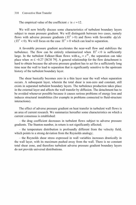
310 Convective Heat Transfer
The empirical value of the coefficient c is c 12.
We will now briefly discuss some characteristics of turbulent boundary layers subject to mean pressure gradient. We will distinguish between two cases, namely flows with adverse pressure gradients ( 0) and flows with favorable dp dx ( 0). We will focus on the case 0 which can lead to separation.
A favorable pressure gradient accelerates the near-wall flow and stabilizes the turbulence. The flow can be entirely relaminarized when 0 is sufficiently large. In the turbulent Falkner-Skan flows with u xm , the separation can take place when m 0.27 [SCH 79]. A general relationship for the flow detachment is hard to obtain because the adverse pressure gradient has to act for a sufficiently long time near the wall to lead to separation that is significantly sensitive to the upstream history of the turbulent boundary layer.
The shear basically becomes zero in a thin layer near the wall when separation occurs. A subsequent layer, wherein the total shear is non-zero and constant, still exists in separated turbulent boundary layers. The turbulence production takes place in the external layer and affects the wall transfer by diffusion. The detachment has to be avoided whenever possible because it causes serious problems of energy loss and induces structural instabilities (for example in problems connected to fluid-structure interactions).
The effect of adverse pressure gradient on heat transfer in turbulent wall flows is an area of current research. We summarize hereafter some characteristics on which a current consensus is established:
– the drag coefficient decreases in turbulent flows subject to adverse pressure gradients. The Stanton number, in return is not significantly affected;
– the temperature distribution is profoundly different from the velocity field, which points to a strong deviation from the Reynolds analogy;
– the Reynolds shear stress expressed in wall variables increases drastically in the wall layer, with its maximum pushed away from the wall. There is no constant total shear zone, and therefore turbulent adverse pressure gradient boundary layers do not provide universal distributions.
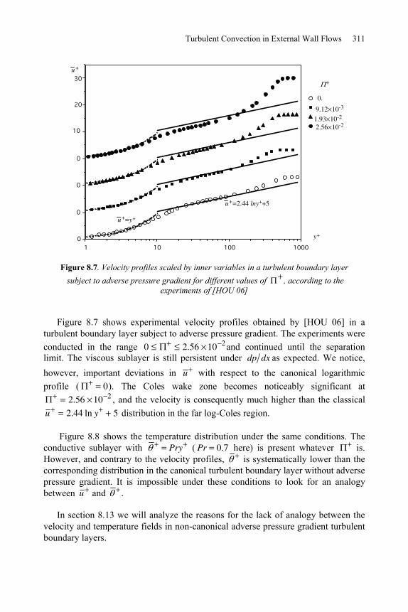
Turbulent Convection in External Wall Flows 311
10001001010
0
0
0
y+
u+
u+=y+
u+=2.44 lny++5
10
20
30
9.12 10-3
0.
1.93 10-2
2.56 10-2
+
Figure 8.7. Velocity profiles scaled by inner variables in a turbulent boundary layer subject to adverse pressure gradient for different values of , according to the
experiments of [HOU 06]
Figure 8.7 shows experimental velocity profiles obtained by [HOU 06] in a turbulent boundary layer subject to adverse pressure gradient. The experiments were conducted in the range 0 2.56 10 2and continued until the separation limit. The viscous sublayer is still persistent under dp dx as expected. We notice, however, important deviations in u with respect to the canonical logarithmic profile ( 0). The Coles wake zone becomes noticeably significant at
2.56 10 2 , and the velocity is consequently much higher than the classical u 2.44 ln y 5 distribution in the far log-Coles region.
Figure 8.8 shows the temperature distribution under the same conditions. The conductive sublayer with Pry ( Pr 0.7 here) is present whatever is. However, and contrary to the velocity profiles, is systematically lower than the corresponding distribution in the canonical turbulent boundary layer without adverse pressure gradient. It is impossible under these conditions to look for an analogy between u and .
In section 8.13 we will analyze the reasons for the lack of analogy between the velocity and temperature fields in non-canonical adverse pressure gradient turbulent boundary layers.
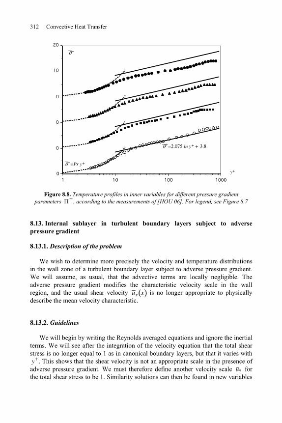
312 Convective Heat Transfer
10001001010
0
0
0
y+
+
+=Pr y+
+=2.075 ln y+ + 3.8
10
20
Figure 8.8. Temperature profiles in inner variables for different pressure gradient parameters , according to the measurements of [HOU 06]. For legend, see Figure 8.7
8.13. Internal sublayer in turbulent boundary layers subject to adverse pressure gradient
8.13.1. Description of the problem
We wish to determine more precisely the velocity and temperature distributions in the wall zone of a turbulent boundary layer subject to adverse pressure gradient. We will assume, as usual, that the advective terms are locally negligible. The adverse pressure gradient modifies the characteristic velocity scale in the wall region, and the usual shear velocity u x is no longer appropriate to physically describe the mean velocity characteristic.
8.13.2. Guidelines
We will begin by writing the Reynolds averaged equations and ignore the inertial terms. We will see after the integration of the velocity equation that the total shear stress is no longer equal to 1 as in canonical boundary layers, but that it varies with y . This shows that the shear velocity is not an appropriate scale in the presence of adverse pressure gradient. We must therefore define another velocity scale u * for the total shear stress to be 1. Similarity solutions can then be found in new variables
Turbulent Convection in External Wall Flows 313
non-dimensionalized by this velocity scale (that will not be a constant). It is therefore proposed to use u * to define an eddy viscosity that will enable us to calculate the velocity distribution in the fully turbulent layer.
The same procedure has to be followed to investigate the temperature distribution. It must be noted that the passive scalar is not directly affected by the adverse pressure gradient in the conductive sublayer. We recommend the use of an eddy-diffusivity closure by using the eddy viscosity that has already been determined and the turbulent Prandtl number. This problem has been studied by [TAR 09].
8.13.3. Solution
The equation that governs the velocity in the inner layer is
01 dp
dx
2u
y2 yu v
where we locally ignored the inertial terms at the left-hand side. Integrating this equation from the wall to some y in the flow gives:
totu
yu v y
dp
dxy w [8.43]
The total shear non-dimensionalized by the local friction velocity u x reads
tot 1dp
dxy 1 y [8.44]
where
1
u 3dp
dx
1
u 3u
du
dx
u
u
3
[8.45]
A new velocity scale, that will be called the pressure gradient velocity u , emerges from [8.45]. Since the Reynolds shear stress is negligible in the viscous sublayer, we have
totu
y1 y
314 Convective Heat Transfer
and
u y12
y 2 [8.46]
which reduces to the classical solution u y in the absence of pressure gradient. We can see that the contribution from dp dx in the viscous sublayer is only slightly important since it is roughly 6% in the case 2.56 10 2 at y 5. The situation is different in the fully turbulent mixing zone wherein the adverse pressure gradient has significant effects, as will be shown below.
The non-dimensionalization of u by the shear velocity leads to similarity solutions in zero adverse pressure gradient turbulent boundary layers through
tot 1. Equation [8.44] clearly indicates that u is no longer a similarity velocity scale under dp dx . Let us consider, instead of u , a new velocity scale defined as
u *2 u 2
u 3
u y [8.47]
that directly takes into account the adverse pressure gradient effects. The total shear given by [8.43] and non-dimensionalized by u * , is:
tot* tot
u *2
1
u *2
u 3
u y u 2 1 [8.48]
Using u * therefore enables us to obtain similarity solutions, as does u in zero pressure gradient turbulent boundary layers. This velocity scale should also intervene in the formulation of eddy viscosity. The turbulent velocity scale is t tut , where
t and ut are, respectively, local turbulent length and velocity scales. Taking as usual t y , ignoring molecular viscosity terms in the fully turbulent mixing zone, and finally introducing ut u *(instead of ut u ), gives rise to
t yu * [8.49]
together with
tot u *2 u v t
u
yyu *
u
y
Turbulent Convection in External Wall Flows 315
resulting in the simple form du dy u * y . The shear scaled by inner variables and u is consequently:
du
dy
u *y
1 y1/ 2
y [8.50]
The integral of this equation gives the velocity distribution in the fully turbulent mixing zone:
u 1
ln y 2 ln1 y 1
22 1 y 1 B [8.51]
B is the constant appearing in the classical logarithmic law ([7.9]).
The pressure gradient does not directly intervene in the temperature distribution, contrary to the velocity field; dp dx indirectly affects the thermal field in the logarithmic region through the eddy viscosity. We have the convection equation that simplifies to
02T
y2v T
y
following the same reasoning as in velocity field, thus ignoring the advective terms. The integration of this equation leads to:
q toty
1
Pr
1
Prtt y 1
We remember that the non-dimensionalization used in the preceding equation is based on the inner variables and u . More precisely:
T w T
T q w
, T q wq wcu
and q totq tot
q w.
In the conductive sublayer, we have
Pry [8.52]
as, incidentally, in the zero pressure gradient turbulent boundary layer.
316 Convective Heat Transfer
However, in the fully turbulent mixing zone, the use of the classical approach of eddy diffusivity results in:
d
dy
Prt
t
Prt
y u *
Prt
y 1 y [8.53]
It would be better at this point to reconsider the discussions leading to [8.53] by directly using the dimensional form of the original expressions in order to convince the reader about the accuracy of the solution obtained here. The transfer equation in the fully turbulent mixing zone is:
c t
Prt
T
yq w
The wall temperature is defined by
T q wq wk
ld
where ld stands for the diffusive length scale (see Chapter 7). Substituting gives:
t
Prt
d
dy
l
ld
ud
u [8.54]
The formulation now depends on the characteristic length scale ld ud , where ud is the diffusive velocity scale in the wall region. We have the choice between ud u and ud u * . Since the viscosity is t yu * (equation [8.49]), using ud u * would result in:
y
Prt
d
dy1 and
Prt ln y C
The effect of the pressure gradient would disappear under these circumstances, except for an eventual dependence through the constant C . The diffusive
velocity scale is therefore the shear velocity u , and not u * , for the thermal boundary layer. Furthermore, the pressure gradient does not intervene in the
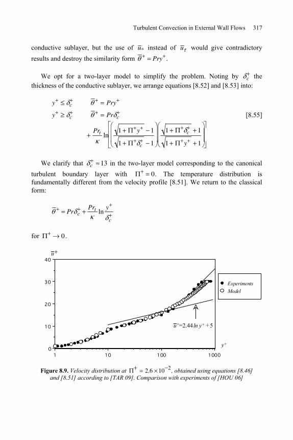
Turbulent Convection in External Wall Flows 317
conductive sublayer, but the use of u * instead of u would give contradictory results and destroy the similarity form Pry .
We opt for a two-layer model to simplify the problem. Noting by c the thickness of the conductive sublayer, we arrange equations [8.52] and [8.53] into:
y c Pry
y c Pr c
Prt ln1 y 1
1 c 1
1 c 1
1 y 1
[8.55]
We clarify that c 13 in the two-layer model corresponding to the canonical turbulent boundary layer with 0. The temperature distribution is fundamentally different from the velocity profile [8.51]. We return to the classical form:
Pr cPrt ln
y
c
for 0 .
10001001010
10
20
30
40
ExperimentsModel
y+
u
u+=2.44 ln y+ + 5
Figure 8.9. Velocity distribution at 2.6 10 2 , obtained using equations [8.46] and [8.51] according to [TAR 09]. Comparison with experiments of [HOU 06]
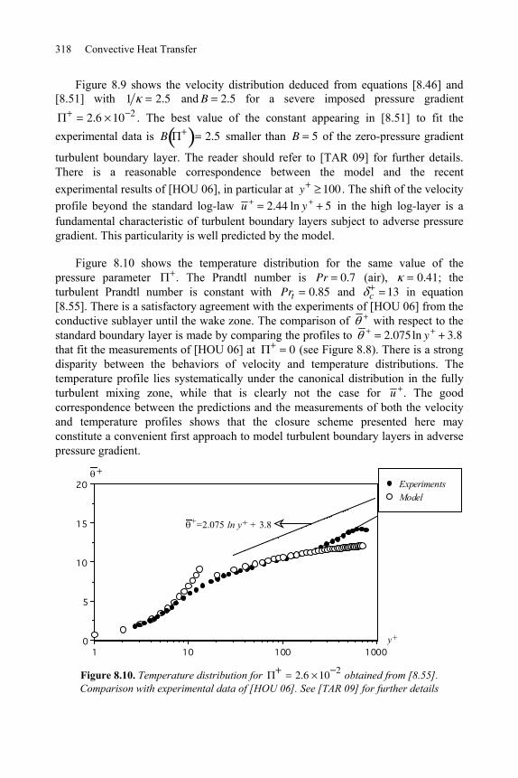
318 Convective Heat Transfer
Figure 8.9 shows the velocity distribution deduced from equations [8.46] and [8.51] with 1 2.5 and B 2.5 for a severe imposed pressure gradient
2.6 10 2 . The best value of the constant appearing in [8.51] to fit the experimental data is B 2.5 smaller than B 5 of the zero-pressure gradient
turbulent boundary layer. The reader should refer to [TAR 09] for further details. There is a reasonable correspondence between the model and the recent experimental results of [HOU 06], in particular at y 100 . The shift of the velocity profile beyond the standard log-law u 2.44 ln y 5 in the high log-layer is a fundamental characteristic of turbulent boundary layers subject to adverse pressure gradient. This particularity is well predicted by the model.
Figure 8.10 shows the temperature distribution for the same value of the pressure parameter . The Prandtl number is Pr 0.7 (air), 0.41; the turbulent Prandtl number is constant with Prt 0.85 and c 13 in equation [8.55]. There is a satisfactory agreement with the experiments of [HOU 06] from the conductive sublayer until the wake zone. The comparison of with respect to the standard boundary layer is made by comparing the profiles to 2.075ln y 3.8 that fit the measurements of [HOU 06] at 0 (see Figure 8.8). There is a strong disparity between the behaviors of velocity and temperature distributions. The temperature profile lies systematically under the canonical distribution in the fully turbulent mixing zone, while that is clearly not the case for u . The good correspondence between the predictions and the measurements of both the velocity and temperature profiles shows that the closure scheme presented here may constitute a convenient first approach to model turbulent boundary layers in adverse pressure gradient.
10001001010
5
10
15
20 ExperimentsModel
y+
+=2.075 ln y+ + 3.8
Figure 8.10. Temperature distribution for 2.6 10 2 obtained from [8.55]. Comparison with experimental data of [HOU 06]. See [TAR 09] for further details
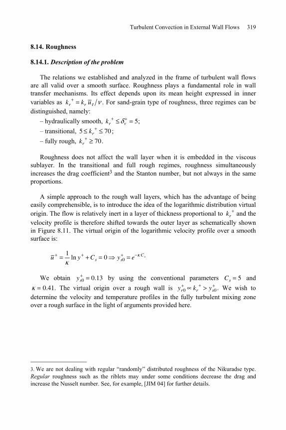
Turbulent Convection in External Wall Flows 319
8.14. Roughness
8.14.1. Description of the problem
The relations we established and analyzed in the frame of turbulent wall flows are all valid over a smooth surface. Roughness plays a fundamental role in wall transfer mechanisms. Its effect depends upon its mean height expressed in inner variables as kr kr u . For sand-grain type of roughness, three regimes can be distinguished, namely:
– hydraulically smooth, kr v 5; – transitional, 5 kr 70 ; – fully rough, kr 70 .
Roughness does not affect the wall layer when it is embedded in the viscous sublayer. In the transitional and full rough regimes, roughness simultaneously increases the drag coefficient3 and the Stanton number, but not always in the same proportions.
A simple approach to the rough wall layers, which has the advantage of being easily comprehensible, is to introduce the idea of the logarithmic distribution virtual origin. The flow is relatively inert in a layer of thickness proportional to kr and the velocity profile is therefore shifted towards the outer layer as schematically shown in Figure 8.11. The virtual origin of the logarithmic velocity profile over a smooth surface is:
u 1
ln y Cs 0 ys0 e Cs
We obtain ys0 0.13 by using the conventional parameters Cs 5 and 0.41. The virtual origin over a rough wall is yr0 kr ys0 . We wish to
determine the velocity and temperature profiles in the fully turbulent mixing zone over a rough surface in the light of arguments provided here.
3. We are not dealing with regular “randomly” distributed roughness of the Nikuradse type. Regular roughness such as the riblets may under some conditions decrease the drag and increase the Nusselt number. See, for example, [JIM 04] for further details.
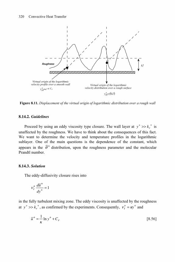
320 Convective Heat Transfer
Virtual origin of the logarithmic velocity profile over a smooth wall Virtual origin of the logarithmic
velocity distribution over a rough surface
Roughnesskr
+
yr0+ =f kr
+
ys0+ =e - Cs
Figure 8.11. Displacement of the virtual origin of logarithmic distribution over a rough wall
8.14.2. Guidelines
Proceed by using an eddy viscosity type closure. The wall layer at y kr is unaffected by the roughness. We have to think about the consequences of this fact. We want to determine the velocity and temperature profiles in the logarithmic sublayer. One of the main questions is the dependence of the constant, which appears in the distribution, upon the roughness parameter and the molecular Prandtl number.
8.14.3. Solution
The eddy-diffusivity closure rises into
tdu
dy1
in the fully turbulent mixing zone. The eddy viscosity is unaffected by the roughness at y kr , as confirmed by the experiments. Consequently, t y and
u 1
ln y Cr [8.56]
Turbulent Convection in External Wall Flows 321
where the integration coefficient Cr is unknown. The virtual origin of distribution [8.56] is a function of kr according to the arguments and discussion in section 8.14.1. With the aid of Figure 8.11 we find
yr0 e Cr kr f kr Cr Cr kr [8.57]
showing that the coefficient Cr depends upon the mean roughness height kr .
The procedure to obtain the temperature distribution is similar. A virtual origin is determined from the logarithmic distribution
Prt ln y C Pr
where we insist on the fact that C is a function of molecular Prandtl number. Following the same reasoning, we find the temperature distribution to be
Prt ln y Cr Pr,kr [8.58]
over a rough wall.
The velocity and temperature profiles over a rough wall are shifted with respect to the standard logarithmic law. The former are often expressed as
rt
r
kPrCyPr
kuCyu
ln
ln1 [8.59]
in the literature. The coefficients C and C refer to the distributions over a smooth wall and u ks C Cr kr together with Pr kr C Cr Pr,kr .
Both u and are positive because the virtual origin is shifted towards the flow from the wall. Thus, the profiles over a rough wall are simply shifted compared to the standard distributions, as schematically shown in Figure 8.12. The experiments indicate that the functions u and Prkr are proportional to
ln kr when kr is sufficiently large [CEB 88]. These functions subsequently
become zero when kr 5 . The drag coefficient and the Stanton number both vary
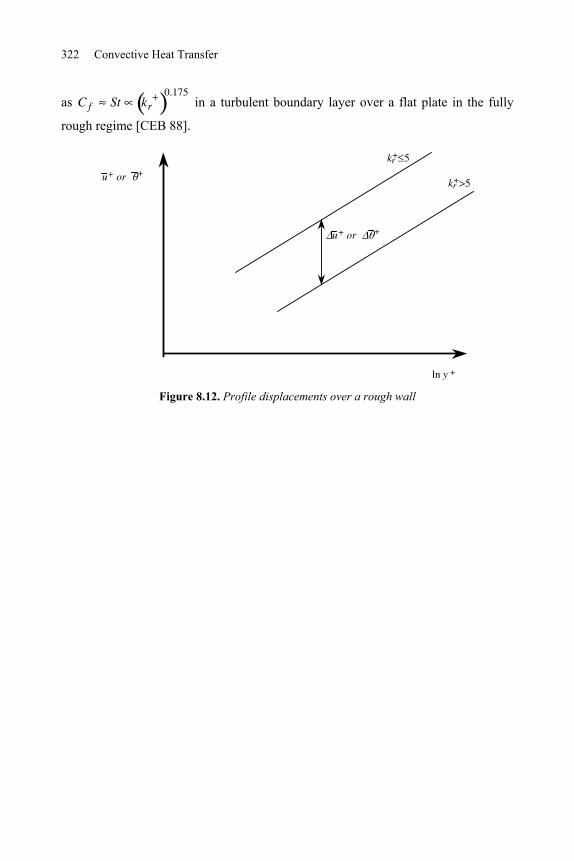
322 Convective Heat Transfer
as C f St kr0.175
in a turbulent boundary layer over a flat plate in the fully
rough regime [CEB 88].
ln y +
u+ or +
u+ or +
kr+>5
kr+ 5
Figure 8.12. Profile displacements over a rough wall
Chapter 9
Turbulent Convection in Free Shear Flows
9.1. Introduction
Free turbulent shear flows play an important role in many industrial and environmental problems. Typical examples can be found in the domains of combustion (turbulent mixing layers), dispersion of pollutants (jets, release of pollutants into rivers, plumes), etc. Turbulent shear layers that are far from walls have very different properties from wall boundary layers and must be treated differently.
However, these various types of free shear flows, although physically different, may be analyzed with the same methods and have closure equations in common. After a general approach that is presented in the next section, thi chapter deals with plumes, turbulent jets, turbulent shear layers and turbulent wakes, and uses the form of various problems.
9.2. General approach of free turbulent shear layers
Let us consider the turbulent interface between a fluid at rest and a plane jet near the nozzle exit, as shown in Figure 9.1. Two shear layers originate at the nozzle sides. They are laminar up to a critical distance and become turbulent farther downstream. Turbulent mixing layers are composed of a row of large structures whose characteristic size grows with the distance x .
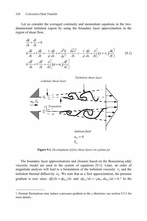
Convective Heat Transfer 324
Let us consider the averaged continuity and momentum equations in the two-dimensional turbulent region by using the boundary layer approximation in the region of shear flow,
u
x
v
y0
u u
xv
u
y
1 dp
dx
2u
y2u v
y
1 dp
dx y tu
y
u T
xv
T
y y tT
y
[9.1]
Turbulent shear layer
Ambient fluid
y
x
Transition
Laminar shear layer
u 0
T
u0 ,T0
Figure 9.1. Development of free shear layers in a plane jet
The boundary layer approximations and closures based on the Boussinesq eddy viscosity model are used in the system of equations [9.1]. Later, an order of magnitude analysis will lead to a formulation of the turbulent viscosity t and the turbulent thermal diffusivity t . We note that as a first approximation, the pressure gradient is zero since dp dx dp dx and dp dx u du dx 0.1 In the
1. Normal fluctuations may induce a pressure gradient in the y-direction; see section 9.5.3 for more details.
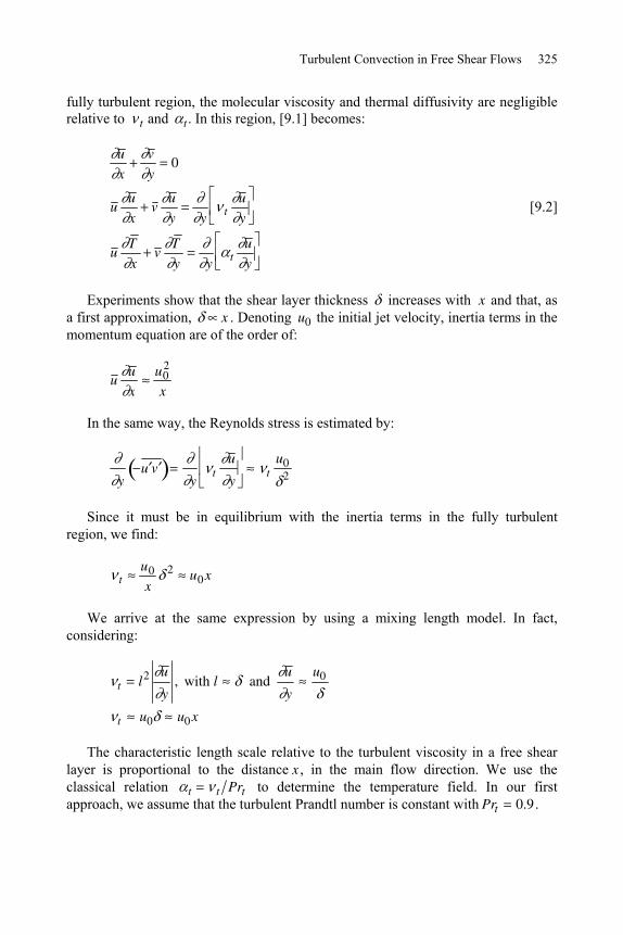
Turbulent Convection in Free Shear Flows 325
fully turbulent region, the molecular viscosity and thermal diffusivity are negligible relative to t and t . In this region, [9.1] becomes:
u
x
v
y0
u u
xv
u
y y tu
y
u T
xv
T
y y tu
y
[9.2]
Experiments show that the shear layer thickness increases with x and that, as a first approximation, x . Denoting u0 the initial jet velocity, inertia terms in the momentum equation are of the order of:
u u
x
u02
x
In the same way, the Reynolds stress is estimated by:
yu v
yt
u
yt
u02
Since it must be in equilibrium with the inertia terms in the fully turbulent region, we find:
tu0
x2 u0x
We arrive at the same expression by using a mixing length model. In fact, considering:
t l2 u
y, with l and
u
y
u0
t u0 u0x
The characteristic length scale relative to the turbulent viscosity in a free shear layer is proportional to the distance x , in the main flow direction. We use the classical relation t t Prt to determine the temperature field. In our first approach, we assume that the turbulent Prandtl number is constant with Prt 0.9 .
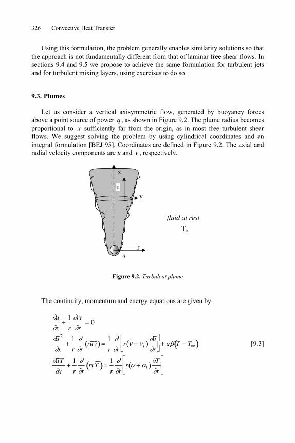
Convective Heat Transfer 326
Using this formulation, the problem generally enables similarity solutions so that the approach is not fundamentally different from that of laminar free shear flows. In sections 9.4 and 9.5 we propose to achieve the same formulation for turbulent jets and for turbulent mixing layers, using exercises to do so.
9.3. Plumes
Let us consider a vertical axisymmetric flow, generated by buoyancy forces above a point source of power q , as shown in Figure 9.2. The plume radius becomes proportional to x sufficiently far from the origin, as in most free turbulent shear flows. We suggest solving the problem by using cylindrical coordinates and an integral formulation [BEJ 95]. Coordinates are defined in Figure 9.2. The axial and radial velocity components are u and v , respectively.
r
uv
fluid at rest T
q
x
Figure 9.2. Turbulent plume
The continuity, momentum and energy equations are given by:
u
x
1
r
rv
r0
u 2
x
1
r rru v
1
r rr t
u
rg T T
u T
x
1
r rrv T
1
r rr t
T
r
[9.3]
Turbulent Convection in Free Shear Flows 327
The continuity equation is multiplied by r and then integrated at given x , from r 0 to a sufficiently large distance from the plume-axis r R , as
d
dxu rdr
0
Rrv R [9.4]
since rv 0 0 for sake of symmetry. Moreover, the momentum equation is also multiplied by r and integrated between the same limits, which gives
2
0 0
R R
tRR
d uu rdr ruv r g T T rdr
dx r
where the conditions of symmetry again have been used. For R , u 0 , which leads to the approximation:
2
0 0
R Rd
u rdr g T T rdrdx
[9.5]
The integration of energy equation, also multiplied by r, yields for the same reasons:
d
dxu T rdr
0
Rrv T
Rr t
T
r R
0 [9.6]
Combining [9.6] with [9.4] and letting R , we obtain the conservation of the flow of enthalpy through any cross-section of height x
0
0du T T rdr
dx
which is a general result for most free turbulent shear flows (see turbulent jets, section 9.4). The energy budget applied to a control domain, including the heat source, is expressed as:
02
u T T rdrc
[9.7]
Convective Heat Transfer 328
The next step of the procedure depends on the shape of the chosen profiles, which is a general feature of integral analysis. [BEJ 95] considers the Gaussian profiles:
u u c expr
b
2
T T T c T expr
bt
2 [9.8]
Equations [9.4], [9.5] and [9.7] enable us to determine the unknowns u c , T c and b, if we are able to model rv R , which remains finite for R . In particular, equation [9.4] gives:
d
dxu cb2 2 rv R
The plume radius satisfies b x , according to observations. We deduce that in a order of magnitude sense rv R u cb . It is then straightforward to show [BEJ 95] that:
u c x 1/ 3
T c T x 5 / 3
9.4. Two-dimensional turbulent jet
9.4.1. Description of the problem
We consider a two-dimensional turbulent jet, as shown in Figure 9.1. The problem consists of determining the necessary conditions for the basic equations to enable similarity solutions for the velocity and temperature fields. We introduce the similarity variable y x , where y is the distance to the jet-axis and x the jet thickness:
– By integrating the momentum and energy equations, show that the flow rates of momentum and enthalpy are constant through any jet cross-section. Calculate the relations relating x to the jet axis-velocity u c x and temperature T c x . Show that x and compare this result to the corresponding law for a laminar jet. Show also that T c T x 1/ 2 .
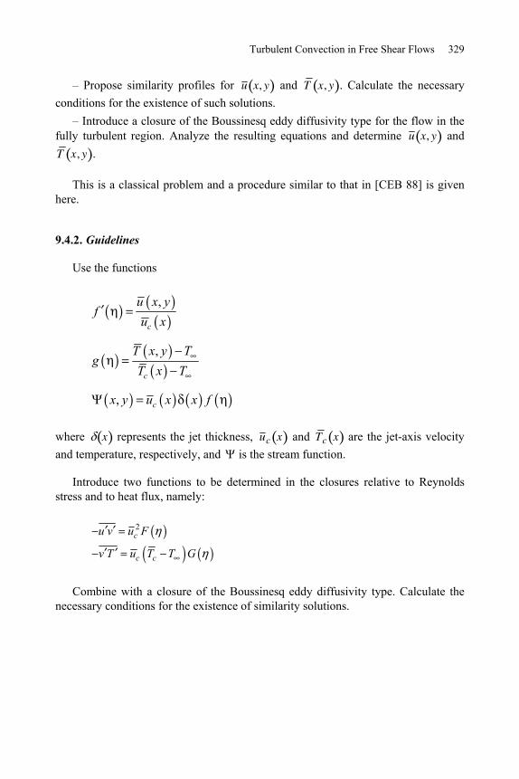
Turbulent Convection in Free Shear Flows 329
– Propose similarity profiles for u x, y and T x, y . Calculate the necessary conditions for the existence of such solutions.
– Introduce a closure of the Boussinesq eddy diffusivity type for the flow in the fully turbulent region. Analyze the resulting equations and determine u x, y and T x, y .
This is a classical problem and a procedure similar to that in [CEB 88] is given here.
9.4.2. Guidelines
Use the functions
,
,
,
c
c
c
u x yf
u x
T x y Tg
T x T
x y u x x f
where x represents the jet thickness, u c x and T c x are the jet-axis velocity and temperature, respectively, and is the stream function.
Introduce two functions to be determined in the closures relative to Reynolds stress and to heat flux, namely:
2c
c c
u v u F
v T u T T G
Combine with a closure of the Boussinesq eddy diffusivity type. Calculate the necessary conditions for the existence of similarity solutions.
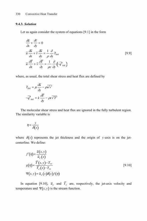
Convective Heat Transfer 330
9.4.3. Solution
Let us again consider the system of equations [9.1] in the form
u
x
v
y0
u u
xv
u
y
1
ytot
u T
xv
T
y
1
c yq tot
[9.9]
where, as usual, the total shear stress and heat flux are defined by
totu
yu v
q tot kT
ycv T
The molecular shear stress and heat flux are ignored in the fully turbulent region. The similarity variable is
y
x
where x represents the jet thickness and the origin of y -axis is on the jet-centerline. We define:
f u x, y
u c x
gT x, y T
T c x T
x, y u c x x f
[9.10]
In equation [9.10], u c and T c are, respectively, the jet-axis velocity and temperature and x, y is the stream function.
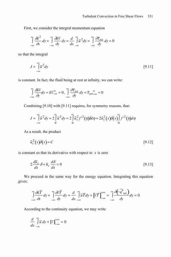
Turbulent Convection in Free Shear Flows 331
First, we consider the integral momentum equation
u 2
xdy
u v
ydy
d
dxu 2dy tot
ydy 0
so that the integral
J u 2dy [9.11]
is constant. In fact, the fluid being at rest at infinity, we can write:
u v
ydy u v 0, tot
ydy tot 0
Combining [9.10] with [9.11] requires, for symmetry reasons, that:
J u 2dy 2 u 2
0dy 2 u c
2
0f 2 d 2u c
2 x x f 2 d0
As a result, the product
u c2 x x C [9.12]
is constant so that its derivative with respect to x is zero
2du cdx
u cd
dx0 [9.13]
We proceed in the same way for the energy equation. Integrating this equation gives:
u T
xdy
v T
ydy
d
dxu T dy v T
q tot
ydy 0
According to the continuity equation, we may write
d
dxu dy v 0
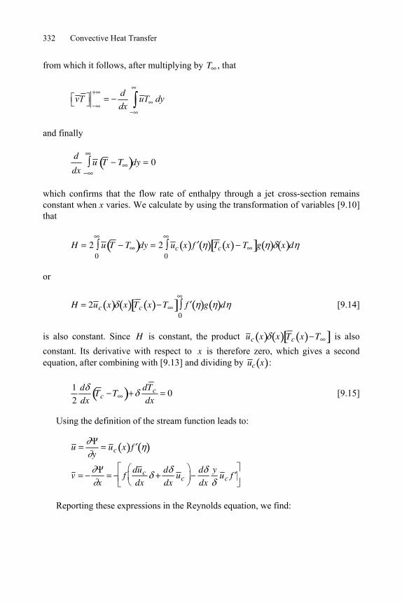
Convective Heat Transfer 332
from which it follows, after multiplying by T , that
dvT uT dy
dx
and finally
d
dxu T T dy 0
which confirms that the flow rate of enthalpy through a jet cross-section remains constant when x varies. We calculate by using the transformation of variables [9.10] that
H 2 u T T dy 2 u c x f T c x T g x d00
or
H 2u c x x T c x T f g d0
[9.14]
is also constant. Since H is constant, the product u c x x T c x T is also constant. Its derivative with respect to x is therefore zero, which gives a second equation, after combining with [9.13] and dividing by u c x :
1
2
d
dxT c T
dT cdx
0 [9.15]
Using the definition of the stream function leads to:
u y
u c x f
v x
fdu cdx
d
dxu c
d
dx
yu c f
Reporting these expressions in the Reynolds equation, we find:
Turbulent Convection in Free Shear Flows 333
u cdu cdx
f 2 1
2u c
2 d
dxf
f 1 tot
Using the conservation of momentum [9.13], replacing
du cdx
u c2
d
dx
in the above expression and rearranging, we obtain
u c2
2
d
dxf 2 ff
1 tot [9.16]
This expression requires a closure equation for tot and additional assumptions in order to obtain a similarity solution.
We proceed in the same fashion for the energy equation. Combining [9.9] and [9.10], we obtain:
u c f gdT cdx
1
2u c fg
d
dxT c T
1
c
q tot
Combining with equation [9.15], which expresses the conservation of energy, leads to:
x u c xdT cdx
f g1
c
q tot [9.17]
Let us now introduce closure equations for tot and q tot . Using the guidelines given in section 9.4.2, we write
tot u v u c2F
q tot
cv T u c T c T G
which enables us to eliminate u c x in equations [9.16] and [9.17]. Finally, we find:
Convective Heat Transfer 334
1
2
d
dxf 2 ff F 0
x
T c x T
d
dxT c x T f g G 0
[9.18]
These equations enable similarity solutions if: – d dx is independent of x , which requires x . Moreover, since
u c2 x x C according to [9.12], we obtain the law of distribution for the jet-axis
velocity as u c x x 1/ 2. We indicate that, for a laminar plane jet, x2 / 3 and
u c x x 1/ 3 . Turbulence accelerates the jet expansion.
– In these conditions, the energy equation also enables a similarity solution if the jet-axis temperature varies as T c x T xs, where s is a constant. In fact,
u c x1/ 2 and the jet-axis temperature must satisfy T c x T x 1/ 2 so that the integral flow of enthalpy remains constant, according to [9.14].
We choose a closure of the Boussinesq eddy diffusivity type, namely:
tot u c2F t
u
yt
u c f
q tot
cu c T c T G t
Prt
T
yt
PrtT c T
g
Replacing these expressions in [9.18] and rearranging leads to:
u cx
2 t
d
dxf 2 ff f 0
Prt
t
u c2 x
T c x T
d
dxT c x T f g g 0
[9.19]
The necessary conditions for the existence of similarity solutions now clearly appear. The turbulent viscosity must fulfill the condition
t u cd
dx
Turbulent Convection in Free Shear Flows 335
and since x , the necessary condition is t u c u c x . We recover the behavior of t as obtained by the order of magnitude analysis in section 9.2.
The associated boundary conditions are:
f g 0 (u 0, T T )
0 f 0 (v 0), f 0 (u
y0), g 0 (
T
y0)
[9.20]
In practice, the jet thickness is defined as the distance to the axis for which u 0.5u c . Experiments show that:
t x 0.037u c
A semi-empirical solution is given by [CEB 88]:
u
u c xsech2 0.881
T x, y T
T c x Tsech 0.881
2Prt
[9.21]
For Prt 1, the velocity and temperature profiles become identical.
9.5. Mixing layer
9.5.1. Description of the problem
Two irrotational streams with uniform velocities and temperatures U1, T1 and U2, T2 join and mix in the downstream direction, as shown in Figure 9.3. For
Reu x
7 104
where u U1 U2 2 , the flow becomes turbulent. Determine the velocity and temperature distributions in the fully turbulent mixing layer and demonstrate the existence of similarity solutions.
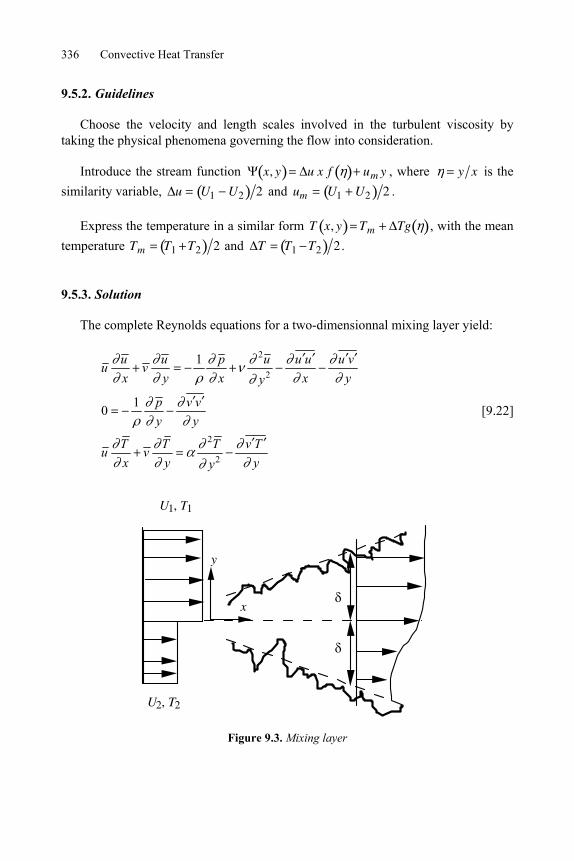
Convective Heat Transfer 336
9.5.2. Guidelines
Choose the velocity and length scales involved in the turbulent viscosity by taking the physical phenomena governing the flow into consideration.
Introduce the stream function x, y u x f um y , where y x is the similarity variable, u U1 U2 2 and um U1 U2 2 .
Express the temperature in a similar form T x, y Tm Tg , with the mean temperature Tm T1 T2 2 and T T1 T2 2 .
9.5.3. Solution
The complete Reynolds equations for a two-dimensionnal mixing layer yield:
2
2
2
2
1
10
u u p u u u u vu v
x y x x yy
p v vy y
T T T v Tu v
x y yy
[9.22]
U1, T1
U2, T2
y
x
Figure 9.3. Mixing layer
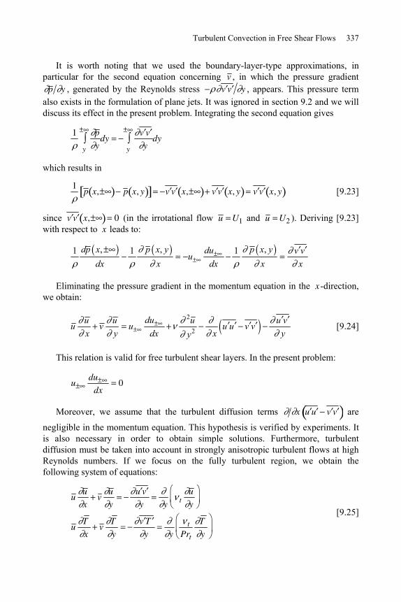
Turbulent Convection in Free Shear Flows 337
It is worth noting that we used the boundary-layer-type approximations, in particular for the second equation concerning v , in which the pressure gradient
p y , generated by the Reynolds stress v v y , appears. This pressure term also exists in the formulation of plane jets. It was ignored in section 9.2 and we will discuss its effect in the present problem. Integrating the second equation gives
1 p
yy
dyv v
yy
dy
which results in
1p x, p x, y v v x, v v x, y v v x, y [9.23]
since v v x, 0 (in the irrotational flow u U1 and u U2 ). Deriving [9.23] with respect to x leads to:
, , ,1 1 1dp x p x y p x ydu v vu
dx x dx x x
Eliminating the pressure gradient in the momentum equation in the x -direction, we obtain:
2
2duu u u u v
u v u u u v vx y dx x yy
[9.24]
This relation is valid for free turbulent shear layers. In the present problem:
udu
dx0
Moreover, we assume that the turbulent diffusion terms x u u v v are
negligible in the momentum equation. This hypothesis is verified by experiments. It is also necessary in order to obtain simple solutions. Furthermore, turbulent diffusion must be taken into account in strongly anisotropic turbulent flows at high Reynolds numbers. If we focus on the fully turbulent region, we obtain the following system of equations:
u u
xv
u
y
u v
y y tu
y
u T
xv
T
y
v T
y yt
Prt
T
y
[9.25]
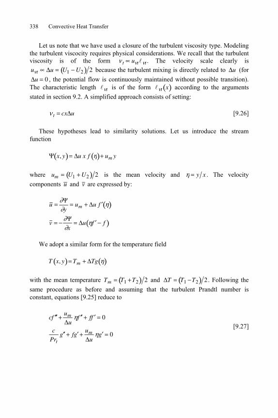
Convective Heat Transfer 338
Let us note that we have used a closure of the turbulent viscosity type. Modeling the turbulent viscocity requires physical considerations. We recall that the turbulent viscosity is of the form t u t t . The velocity scale clearly is u t u U1 U2 2 because the turbulent mixing is directly related to u (for
u 0 , the potential flow is continuously maintained without possible transition). The characteristic length t is of the form t x according to the arguments stated in section 9.2. A simplified approach consists of setting:
t cx u [9.26]
These hypotheses lead to similarity solutions. Let us introduce the stream function
x, y u x f um y
where um U1 U2 2 is the mean velocity and y x . The velocity components u and v are expressed by:
u y
um u f
v x
u f f
We adopt a similar form for the temperature field
T x, y Tm Tg
with the mean temperature Tm T1 T2 2 and T T1 T2 2 . Following the same procedure as before and assuming that the turbulent Prandtl number is constant, equations [9.25] reduce to
cf um
uf ff 0
c
Prtg fg
um
ug 0
[9.27]
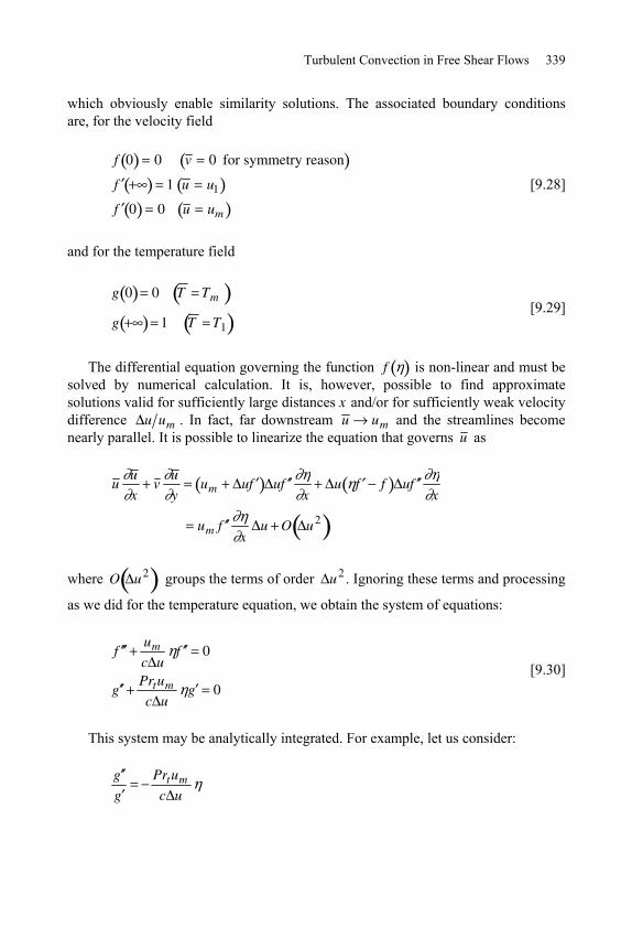
Turbulent Convection in Free Shear Flows 339
which obviously enable similarity solutions. The associated boundary conditions are, for the velocity field
f 0 0 v 0 for symmetry reason
f 1 u u1
f 0 0 u um
[9.28]
and for the temperature field
g 0 0 T Tm
g 1 T T1
[9.29]
The differential equation governing the function f is non-linear and must be solved by numerical calculation. It is, however, possible to find approximate solutions valid for sufficiently large distances x and/or for sufficiently weak velocity difference u um . In fact, far downstream u um and the streamlines become nearly parallel. It is possible to linearize the equation that governs u as
u u
xv
u
yum uf uf
xu f f uf
x
um f x
u O u2
where O u2 groups the terms of order u2 . Ignoring these terms and processing
as we did for the temperature equation, we obtain the system of equations:
f um
c uf 0
g Prtum
c ug 0
[9.30]
This system may be analytically integrated. For example, let us consider:
g
g
Prtum
c u
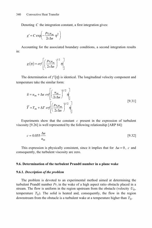
Convective Heat Transfer 340
Denoting C the integration constant, a first integration gives:
g C expPrtum
2c u2
Accounting for the associated boundary conditions, a second integration results in:
1/2
2t mPr u
g erfc u
The determination of f is identical. The longitudinal velocity component and temperature take the similar form:
u um u erfum
2c u
1/ 2
T Tm T erfPrtum
2c u
1/ 2 [9.31]
Experiments show that the constant c present in the expression of turbulent viscosity [9.26] is well represented by the following relationship [ARP 84]:
c 0.055u
um
[9.32]
This expression is physically consistent, since it implies that for u 0 , c and consequently, the turbulent viscosity are zero.
9.6. Determination of the turbulent Prandtl number in a plane wake
9.6.1. Description of the problem
The problem is devoted to an experimental method aimed at determining the turbulent Prandtl number Prt in the wake of a high aspect ratio obstacle placed in a stream. The flow is uniform in the region upstream from the obstacle (velocity U0 , temperature T0). The solid is heated and, consequently, the flow in the region downstream from the obstacle is a turbulent wake at a temperature higher than T0 .
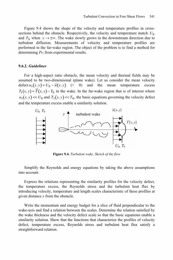
Turbulent Convection in Free Shear Flows 341
Figure 9.4 shows the shape of the velocity and temperature profiles in cross-sections behind the obstacle. Respectively, the velocity and temperature match U0 and T0 when y . The wake slowly grows in the downstream direction due to turbulent diffusion. Measurements of velocity and temperature profiles are performed in the far-wake region. The object of the problem is to find a method for determining Prt from experimental results.
9.6.2. Guidelines
For a high-aspect ratio obstacle, the mean velocity and thermal fields may be assumed to be two-dimensional (plane wake). Let us consider the mean velocity defect u1 x, y U0 u x, y (> 0) and the mean temperature excess T1 x, y T x, y T0 in the wake. In the far-wake region that is of interest where u1 x, y U0 and T1 x, y T0 , the basic equations governing the velocity defect and the temperature excess enable a similarity solution.
Figure 9.4. Turbulent wake. Sketch of the flow
Simplify the Reynolds and energy equations by taking the above assumptions into account.
Express the relations representing the similarity profiles for the velocity defect, the temperature excess, the Reynolds stress and the turbulent heat flux by introducing velocity, temperature and length scales characteristic of these profiles at given distance x from the obstacle.
Write the momentum and energy budget for a slice of fluid perpendicular to the wake-axis and find a relation between the scales. Determine the relation satisfied by the wake thickness and the velocity defect scale so that the basic equations enable a similarity solution. Show that the functions that characterize the profiles of velocity defect, temperature excess, Reynolds stress and turbulent heat flux satisfy a straightforward relation.
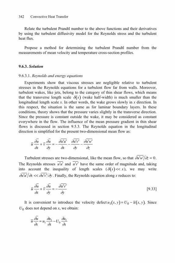
Convective Heat Transfer 342
Relate the turbulent Prandtl number to the above functions and their derivatives by using the turbulent diffusivity model for the Reynolds stress and the turbulent heat flux.
Propose a method for determining the turbulent Prandtl number from the measurements of mean velocity and temperature cross-section profiles.
9.6.3. Solution
9.6.3.1. Reynolds and energy equations
Experiments show that viscous stresses are negligible relative to turbulent stresses in the Reynolds equations for a turbulent flow far from walls. Moreover, turbulent wakes, like jets, belong to the category of thin shear flows, which means that the transverse length scale x (wake half-width) is much smaller than the longitudinal length scale x. In other words, the wake grows slowly in x direction. In this respect, the situation is the same as for laminar boundary layers. In these conditions, theory shows that the pressure varies slightly in the transverse direction. Since the pressure is constant outside the wake, it may be considered as constant everywhere in the flow. The influence of the mean pressure gradient in thin shear flows is discussed in section 9.5.3. The Reynolds equation in the longitudinal direction is simplified for the present two-dimensional mean flow as:
u u
xv
u
y
u u
x
u v
y
u w
z
Turbulent stresses are two-dimensional, like the mean flow, so that u w z 0 . The Reynolds stresses u u and u v have the same order of magnitude and, taking into account the inequality of length scales ( x x ), we may write
u u x u v y . Finally, the Reynolds equation along x reduces to:
u u
xv
u
y
u v
y [9.33]
It is convenient to introduce the velocity defect u1 x, y U0 u x, y . Since U0 does not depend on x, we obtain:
u u
xu1
u1
xU0
u1
x
Turbulent Convection in Free Shear Flows 343
Moreover, since u1 x, y U0, only the second term is retained in the above equation.
After introducing the velocity defect, the continuity equation yields:
u1
x
v
y0
Denoting U1 the velocity defect scale in a given cross-section, the order of magnitude of the mean transverse velocity is V U1 x . The two terms of the left-hand side of equation [9.33] thus have the respective order of magnitude
U0 U1 x U12 x
so that the inertia term corresponding to v is negligible relative to the first term corresponding to u . Finally, the longitudinal Reynolds equation further simplifies as:
U0u1
x
u v
y [9.34]
The same calculations applied to the energy equation lead to:
U0T1
x
v T
y [9.35]
9.6.3.2. Momentum and energy budget for a slice of fluid
We consider a slice of fluid delimited by two cross-sections of abscissa x and x dx and by the plane of symmetry of the wake (Figure 9.5). The conservation of flow rate shows that the flow necessarily has a velocity component v at infinity to compensate for the difference in the flow rate between the two cross-sections.
Figure 9.5. Turbulent wake. Control domain
T0y U0
v
x
x +dx
O
x
Convective Heat Transfer 344
In fact, for the control domain the flow rate budget reads
0, 0d
u x y dy dx v dxdx
so that v xd
dxu x, y dy0 .
This velocity is positive since the region of velocity defect extends more and more in the downstream direction. For the same control domain, since the pressure is constant everywhere in the flow, the momentum budget yields
d
dxu 2 x, y dy0 U0v 0
or d
dxu x, y u x, y U0 dy0 0
when the conservation of flow rate is accounted for.
Introducing the velocity defect and noting that u1 U0 , we obtain
U0d
dxu1 x, y dy0 0
u1 x, y dy0 C1 [9.36]
The same procedure is used for the energy budget applied to the same control domain. Ignoring longitudinal heat flux, the flow rate of enthalpy is invariant through every cross-section. Normalizing the fluid temperature by the external temperature, it follows that
d
dxC pu x, y T x, y T0 dy0 0
and consequently
T1 x, y dy0 C2 [9.37]
Turbulent Convection in Free Shear Flows 345
9.6.3.3. Similarity solution
Let us assume that equations [9.34] and [9.35] enable a solution of the form
u1 x, y
Ua xf1 [9.38]
T1 x, y
Ta xf2 [9.39]
u v x, y
Ua2 x
g1 [9.40]
v T x, y
Ua x Ta xg2 [9.41]
where Ua x and Ta x represent, respectively, the velocity defect and the temperature excess on the wake-axis. The distance to the symmetry-axis is normalized by the wake half-width as y x .
Substituting into the system [9.36] and [9.37], we obtain
Ua x x f1 d0 C1
from which it follows that
Ua x x c1 [9.42]
and taking equation [9.37] into account
Ta x x f2 d0 C2
Taking the functions of x only out of the integral, we find:
Ta x x c2 [9.43]
Convective Heat Transfer 346
The above relations lead to:
Ua x
Ua x
Ta x
Ta x
x
x [9.44]
Substituting the assumed similarity solution [9.38]-[9.41] into the system [9.34]-[9.35] gives:
U0
Ua x
Ua x
Ua xx f1 x f1 g1 [9.45]
U0
Ua x
Ta x
Ta xx f2 x f2 g2 [9.46]
Relations [9.44] are introduced into the two equations immediately above to obtain:
U0 x
Ua xf1 f1 g1 [9.47]
U0 x
Ua xf2 f2 g2 [9.48]
Clearly, a similarity solution is possible only if:
U0 x
Ua xc3 [9.49]
The following calculation is not necessary to determine the turbulent Prandtl number; it gives, however, the far-wake laws for Ua x , Ta x and x . Combining [9.42] and [9.49], we obtain
U0 x x c1c3
x2c1c3
U0
x [9.50]
where x refers to a virtual origin.
Turbulent Convection in Free Shear Flows 347
The distribution of the velocity defect and temperature excess on the symmetry-axis of the wake are deduced from the previous equations:
Ua xc1U0
2c3x [9.51]
Ta xc2
2U0
2c1c3x [9.52]
Let us again consider equations [9.47] and [9.48]. Substituting [9.49] into these equations, we obtain
c3 f1 f1 g1 [9.53]
c3 f2 f2 g2 [9.54]
which are integrated as
c3 f1 g1 d1
c3 f2 g2 d2
On the symmetry-axis of the wake ( 0), the Reynolds stress u v and the turbulent heat flux v T are zero, simultaneously with the mean velocity and temperature gradients (turbulent diffusivity model, as will be seen later). Furthermore, according to expressions [9.38] and [9.39], f1 0 f2 0 1. As a result, we find that the two constants d1 and d2 are zero. It follows that:
f1f2
g1
g2
[9.55]
The definition of turbulent diffusivities is:
u v t u y
v T t T y
Convective Heat Transfer 348
These relations may be transformed by using the similarity solution:
Ua2 x g1 t
Ua x
xf1
Ua x Ta x g2 tTa x
xf2
Dividing these two relations side by side, we find:
g1
g2
t
t
f1
f2
[9.56]
We recall that the turbulent Prandtl number is the ratio of the momentum to the heat diffusivity Prt t t . Combining [9.55] and [9.56] the final result is:
Prtf1f2
f2
f1
[9.57]
This relation shows that the turbulent Prandtl number may be determined experimentally by using measured mean velocity and temperature profiles. In the first step, the velocity defect Ua x and the temperature excess Ta x are determined on the symmetry-axis of the wake in a given cross-section. The profiles are then normalized as in equations [9.38] and [9.39] for numerically calculating the functions f1 , f2 and their derivatives, which are reported in [9.57] in order to obtain finally Prt .
9.7. Regulation of temperature
9.7.1. Description of the problem
In many facilities, it is necessary to regulate the temperature of the working fluid for stable use conditions. We propose to examine the case of a closed-loop circuit including a system for heating and regulating the fluid temperature. In order to damp temperature fluctuations generated by the heating system, the circuit also includes a cylindrical tank of diameter D and length L, which plays the role of a hydraulic capacity. This tank is assumed to be perfectly insulated. The working fluid is water.
The fluid flow rate Q0 in the circuit is assumed to be constant with time. Water flows into the tank at temperature Ti t through a circular opening and then inside the tank as a turbulent axisymmetric jet. Finally, the liquid exits at temperature Te t
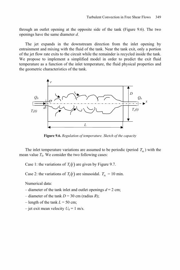
Turbulent Convection in Free Shear Flows 349
through an outlet opening at the opposite side of the tank (Figure 9.6). The two openings have the same diameter d.
The jet expands in the downstream direction from the inlet opening by entrainment and mixing with the fluid of the tank. Near the tank exit, only a portion of the jet flow rate exits to the circuit while the remainder is recycled inside the tank. We propose to implement a simplified model in order to predict the exit fluid temperature as a function of the inlet temperature, the fluid physical properties and the geometric characteristics of the tank.
Figure 9.6. Regulation of temperature. Sketch of the capacity
The inlet temperature variations are assumed to be periodic (period T ) with the mean value T0. We consider the two following cases:
Case 1: the variations of Ti t are given by Figure 9.7.
Case 2: the variations of Ti t are sinusoidal. T = 10 min.
Numerical data: – diameter of the tank inlet and outlet openings d = 2 cm; – diameter of the tank D = 30 cm (radius R); – length of the tank L = 50 cm; – jet exit mean velocity U0 = 1 m/s.
Q0 Q0
d
D
L
Ti(t) Te(t)
x
r
O
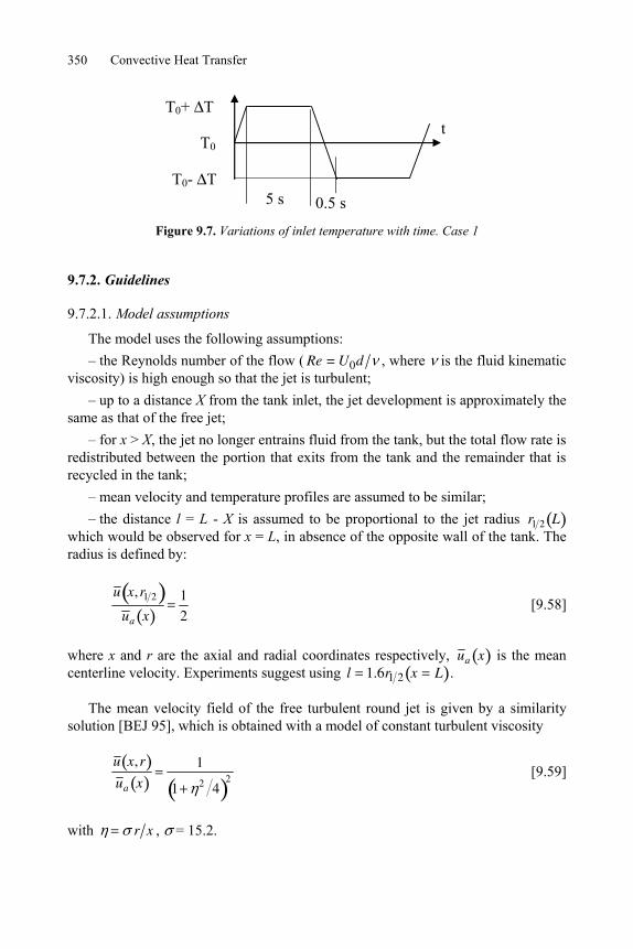
Convective Heat Transfer 350
5 s 0.5 s
T0
T0+ T
T0- T
t
Figure 9.7. Variations of inlet temperature with time. Case 1
9.7.2. Guidelines
9.7.2.1. Model assumptions
The model uses the following assumptions: – the Reynolds number of the flow ( Re = U0d , where is the fluid kinematic
viscosity) is high enough so that the jet is turbulent; – up to a distance X from the tank inlet, the jet development is approximately the
same as that of the free jet; – for x > X, the jet no longer entrains fluid from the tank, but the total flow rate is
redistributed between the portion that exits from the tank and the remainder that is recycled in the tank;
– mean velocity and temperature profiles are assumed to be similar; – the distance l = L - X is assumed to be proportional to the jet radius r1 2 L
which would be observed for x = L, in absence of the opposite wall of the tank. The radius is defined by:
u x,r1 2
u a x
1
2 [9.58]
where x and r are the axial and radial coordinates respectively, u a x is the mean centerline velocity. Experiments suggest using l 1.6r1 2 x L .
The mean velocity field of the free turbulent round jet is given by a similarity solution [BEJ 95], which is obtained with a model of constant turbulent viscosity
u x,r
u a x
1
1 2 42
[9.59]
with r x , = 15.2.
Turbulent Convection in Free Shear Flows 351
9.7.2.2. Suggested approach
Develop the hydraulic model to represent the flow in the tank. Complete the theory of the turbulent free jet. Using the momentum budget, determine the laws of mean centerline velocity and jet flow rate as a function of the distance to the tank inlet.
Estimate the characterictic time constants for the thermal regime of the jet and the tank.
Propose a model for calculating the fluid exit temperature Te t in the two cases of the problem.
9.7.3. Solution
9.7.3.1. Hydraulic model
9.7.3.1.1. Turbulent jet development
Up to the distance X from the tank inlet, it is assumed that the jet development is not influenced by confinment. First, we calculate the free jet radius for x = L. According to relation [9.59], the dimensionless radius 1 2 is given by
1
1 2 42
1
2
or 1/2 = 1.287. The resulting radius is r1 2 x 1 2 x = 0.085 x.
The jet therefore expands linearly. For x = L, we obtain r1 2 L 4.25 cm.
The distribution of mean centerline velocity is deduced from the momentum budget in a jet cross-section. With the assumption that the flow is axisymmetric with respect to Ox-axis, the flow of momentum J through a tank cross-section is given by:
J 2 u 2 x, r0R rdr
Ignoring the presence of the walls and the recycled back flow, the mean axial velocity distribution is given by [9.59] in a tank cross-section so that the previous equation becomes:
J 2 u a2 x
x2
21 2 4
40d
Convective Heat Transfer 352
The calculation of the integral is straightforward by setting u 1 2 4 and gives the resulting value 2/3. Finally:
J4
3u a
2 xx2
2
In the turbulent jet theory, the mean pressure is uniform in the reservoir, which is assumed to have very large dimensions relative to the jet diameter. As a result, the flow of momentum is constant in any jet cross-section. We assume that the same result holds in the tank up to the abscissa X. J is also calculated at the tank inlet.
J U02 d2
4
where the initial jet velocity U0 is assumed to be uniform in the tank inlet. Equaling the two expressions of J, we find:
U0
u a x
4
3
x
d0.152
x
d [9.60]
The mean centerline velocity is inversely proportional to the distance x. It is worth noting that this law only holds in the region of similar cross-section velocity profiles, in other words where the velocity is given by equation [9.59]. In fact, there is a fictitious origin x0 for the jet, which depends on the boundary conditions at the tank inlet. In the present very simplified model, the shift in the jet origin x0 is ignored. It could be accounted for in law [9.60].
The jet flow rate in a cross-section limited to the radius r is calculated by again using velocity distribution [9.59].
Q x,r 2 u x,r0
rrdr = 2 u a x
x2
21 2 4
20
r xd
The calculation of the integral is again straightforward by setting u 1 2 4 and we obtain:
Q x,r 4 u a xx2
2
r x2
4 r x2
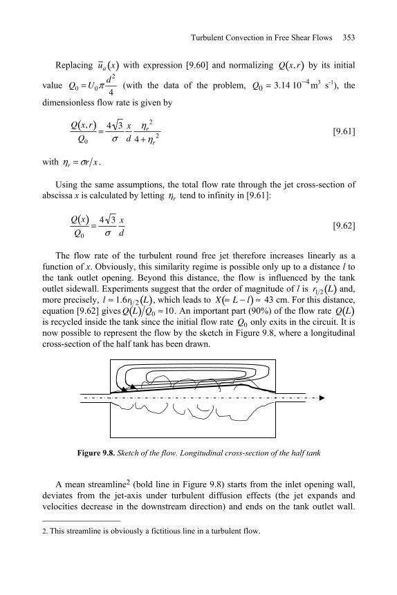
Turbulent Convection in Free Shear Flows 353
Replacing u a x with expression [9.60] and normalizing Q x,r by its initial
value Q0 U0d2
4 (with the data of the problem, Q0 3.14 10 4 m3 s-1), the
dimensionless flow rate is given by
Q x,r
Q0
4 3 x
dr
2
4 r2
[9.61]
with r r x .
Using the same assumptions, the total flow rate through the jet cross-section of abscissa x is calculated by letting r tend to infinity in [9.61]:
Q x
Q0
4 3 x
d [9.62]
The flow rate of the turbulent round free jet therefore increases linearly as a function of x. Obviously, this similarity regime is possible only up to a distance l to the tank outlet opening. Beyond this distance, the flow is influenced by the tank outlet sidewall. Experiments suggest that the order of magnitude of l is r1 2 L and, more precisely, l 1.6r1 2 L , which leads to X L l 43 cm. For this distance, equation [9.62] gives Q L Q0 10. An important part (90%) of the flow rate Q L is recycled inside the tank since the initial flow rate Q0 only exits in the circuit. It is now possible to represent the flow by the sketch in Figure 9.8, where a longitudinal cross-section of the half tank has been drawn.
Figure 9.8. Sketch of the flow. Longitudinal cross-section of the half tank
A mean streamline2 (bold line in Figure 9.8) starts from the inlet opening wall, deviates from the jet-axis under turbulent diffusion effects (the jet expands and velocities decrease in the downstream direction) and ends on the tank outlet wall. 2. This streamline is obviously a fictitious line in a turbulent flow.
Convective Heat Transfer 354
The area open for the recycled flow is a cylindrical annulus, delimited by the tank lateral wall and the jet boundary. Its smallest value is in the downstream region of the jet. In the most unfavorable conditions for the model, the recycled flow rate 9 Q0
passes through an area of the order of 0.152 0.042 , where the jet radius has
been estimated as r1 2 L . The corresponding backward bulk velocity is then
9Q0 0.152 0.042 0.04 m s-1. In the same region ( x L), the jet centerline
velocity is of the order of 0.3 m s-1, according to [9.60]. In the upstream region of the tank (x < X), the area open to the backward flow is larger than in the previous calculation and the backward flow rate is smaller than in the corresponding cross-section leading to smaller backward velocities. These estimations suggest that the backward velocities are small enough relative to the jet velocities so that the jet development is well described by equations [9.59] to [9.62].
9.7.3.2. Thermal model
9.7.3.2.1. Time constants
When the jet initial temperature varies with time, heat transfer associated with the flow in the tank involves two time constants related to two different phenomena.
– On the one hand, the jet convects the information that the inlet conditions vary with time. The time response of the jet associated with this physical phenomenon is the travel time of a fluid particle in the tank. On length L, this time is of the order of:
ttr L U0 = 0.5 s
In fact, this order of magnitude overestimates the time taken by a particle to flow across the tank since the fluid velocity decreases in the downstream direction. Restricting the calculation to a fluid particle on the jet-axis, the travel time is easily calculated as
ttr dx u a x0
L =
0.152
U0
x
ddx0
L = 0.152L
2U0
L
d
where equation [9.60] has been taken into account.
With the numerical data of the problem:
ttr 1 s [9.63]
– On the other hand, the tank fluid temperature varies under the influence of the backward flow. The associated velocities being much smaller than those in the jet, the time response of the water tank is much larger than ttr .
Turbulent Convection in Free Shear Flows 355
The order of magnitude of this response time is estimated by the global energy equation applied to the tank. Denoting qi and qe the inlet flow and exit flow of enthalpy, respectively, and Tr , the mean fluid temperature in the tank, the energy budget reads:
c R2LdTr
dtqi qe
Assuming that the temperature is uniform in the outlet opening, the right-hand side is equal to cQ0 Ti Te . Hence:
R2LdTr
dtQ0 Ti t Te t [9.64]
As a first approximation, the tank time response is calculated from [9.64] and estimated by:
trR2L
Q0
112 s [9.65]
It is worth noting that tr is the ratio of the tank volume to the jet flow rate. As a first approximation, the mean fluid temperature Tr in the tank is not distinguished from the temperature of the back flow.
The model of heat transfer to be implemented depends on the order of magnitude of the period T of the inlet fluid temperature variations compared to the two time constants found above.
If T < ttr or T ttr, the time variations of the jet temperature field must be taken into account. In other words, the unsteady term T t must be retained in the energy equation in turbulent regime. It is then necessary to consider phase averages < g > instead of the classical time averages in turbulence theory.
If ttr << T << tr , the jet may be considered to be in quasi-steady thermal regime, i.e. the jet temperature field is established at every instant. Moreover, the variations of Ti t being much faster than the time response of the tank tr , the temperature Tr in the tank cannot vary during a period T .
If tr < T or T tr , we must consider that the tank temperature varies as a whole with time.
Convective Heat Transfer 356
9.7.3.2.2. Model 1
We assume that the characteristic parameters of the facility are such that ttr << T << tr . We assume that the flow of enthalpy convected through every jet cross-section is constant along the tank in this quasi-steady regime. We also assume that the tank fluid temperature does not vary outside the jet. It is then equal to the fluid mean inlet temperature T0, which is chosen as temperature reference. The following calculations are conducted at given time.
The flow of enthalpy convected through a jet cross-section of radius r is calculated by
qr x, r c2 u x, r T x, r T00r rdr
c2 u a x T a x T0x2
21 2 4
40r x d
where the mean temperature profile has been assumed to be identical to the mean velocity profile, namely
T x, r T0
T a x T0
1
1 2 42
We find
qr x, r c2 u a x T a x T0x2
2
2
31
1
1 r2 4
3 [9.66]
with r r x .
The flow of enthalpy convected through a tank cross-section is obtained for r :
q x4
3c u a x T a x T0
x2
2 [9.67]
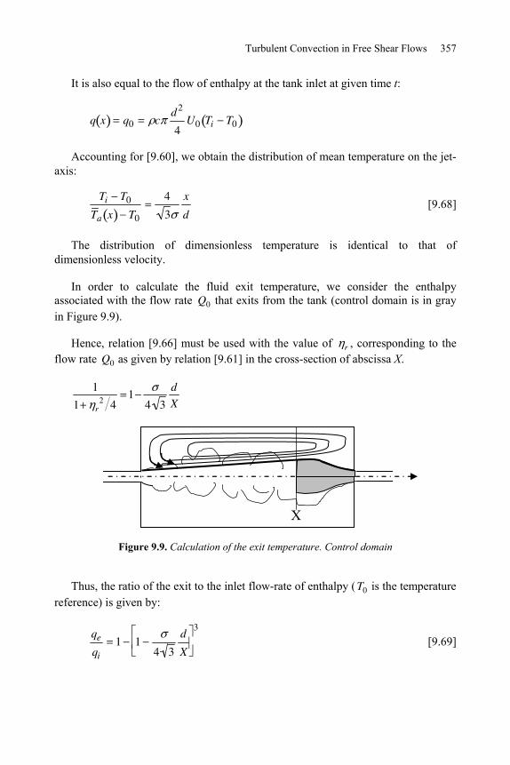
Turbulent Convection in Free Shear Flows 357
It is also equal to the flow of enthalpy at the tank inlet at given time t:
q x q0 cd2
4U0 Ti T0
Accounting for [9.60], we obtain the distribution of mean temperature on the jet-axis:
Ti T0
T a x T0
4
3
x
d [9.68]
The distribution of dimensionless temperature is identical to that of dimensionless velocity.
In order to calculate the fluid exit temperature, we consider the enthalpy associated with the flow rate Q0 that exits from the tank (control domain is in gray in Figure 9.9).
Hence, relation [9.66] must be used with the value of r , corresponding to the flow rate Q0 as given by relation [9.61] in the cross-section of abscissa X.
1
1 r2 4
14 3
d
X
X
Figure 9.9. Calculation of the exit temperature. Control domain
Thus, the ratio of the exit to the inlet flow-rate of enthalpy (T0 is the temperature reference) is given by:
qe
qi
1 14 3
d
X
3
[9.69]
Convective Heat Transfer 358
If X d >> 1, this relation is approximated by:
qe
qi
3
4
d
X [9.70]
With the data of the problem, X d = 21.6, we find:
qe
qi
Te T0
Ti T0
= 0.27 [9.71]
In this model, the temperature fluctuations amplitude at tank exit is 27% of the corresponding amplitude at the inlet.
This model is adapted to case 1, for which the period T (= 10 s) is rather high relative to ttr (1 s) and rather small relative to tr (112 s).
9.7.3.2.3. Model 2
We assume that the characteristic parameters of the facility are such that tr < T or T tr . The period of temperature oscillations being of the same order of magnitude as the time response of the tank or even higher, it is not possible to consider that the tank fluid temperature remains constant with time. The model again assumes that the jet is in quasi-steady regime, but with the fluid temperature outside the jet, denoted Tr t , variable with time as a whole.
With the above assumptions, the jet mean temperature profile reads
T x, r, t Tr t
T a x, t Tr t
1
1 2 42
[9.72]
with the mean temperature distribution on the jet-axis
Ti t Tr t
T a x, t Tr t
4
3
x
d [9.73]
The global energy budget for the whole tank yields
dH dt cQ0 Ti t Te t [9.74]
where H denotes the enthalpy of the liquid contained in the tank.
Turbulent Convection in Free Shear Flows 359
H cT x, r, t dvtank
dx cT x, r, t 2 rdr0R
0L
Introducing temperature law [9.72], the equation becomes:
H dx c Tr tT a x, t Tr t
1 2 42
2x2
2d0
R x0L
The integral is decomposed into two parts. The first part is proportional to Tr and is straightforwardly calculated as:
H1 cTr R2L
The second part is calculated by accounting for [9.73]:
H2 c T a x, t Tr t 2x2
2
R x 2
4 R x 2dx0
L
c Ti t Tr t 3dx R x 2
4 R x 2dx0
L
We set 2x R :
H2 c Ti t Tr t 3dR2
4 1 2d0
2L R
3
8c Ti t Tr t dR2 Ln 1 2L R 2
Thus, finally, denoting a13
8
d
LLn 1 2L R 2 :
H c R2L Tr t a1 Ti t Tr t [9.75]
Convective Heat Transfer 360
This expression of enthalpy is reported in [9.74] to obtain a first equation satisfied by Tr t and Te t
a1dTi
dt1 a1
dTr
dtb Ti Te [9.76]
with b Q0 R2L = 1 tr .
A second equation is obtained by writing the enthalpy budget on the same control domain as in model 1 (Figure 9.9)
qr X, r, t c2 u x, r T X, r, t Tr t0r rdr = cQ0 Te t Tr t
where Tr t has been chosen as reference temperature instead of T0 to calculate the integral like in the first model. The calculation is identical to that of model 1 so that we find, as in [9.71],
Te t Tr t
Ti t Tr tc1 [9.77]
with c1 = 0.27 for X d = 21.6.
Eliminating Tr t between [9.76] and [9.77], we obtain the equation satisfied by Te t
adTe
dtbTe c
dTi
dtbTi [9.78]
with a1 a1
1 c1
, c ac1 a1.
The case of sinusoidal variations of inlet temperature is easily calculated:
Ti t T0 Ai cos t , with 2 T
We find
Te t T0 Ae cos t [9.79]
with the damping factor Ae Ai cos m sin , and the phase shift given
by tan1 mn
n m, where we have set m a b, n b c .
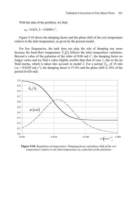
Turbulent Convection in Free Shear Flows 361
With the data of the problem, we find:
a1= 0.023, b = 0.0089 s-1.
Figure 9.10 shows the damping factor and the phase shift of the exit temperature relative to the inlet temperature, as given by the present model.
For low frequencies, the tank does not play the role of damping any more because the back-flow temperature Tr t follows the inlet temperature variations. Beyond a value of the pulsation of the order of 0.06 rad s-1, the damping factor no longer varies and we find a value slightly smaller than that of case 1, due to the jet fluid inertia, which is taken into account in model 2. For a period T of 10 min ( = 0.0105 rad s-1), the damping factor is 57.6% and the phase shift is 10% of the period (0.626 rad).
0.0
0.1
0.2
0.3
0.4
0.5
0.6
0.7
0.8
0.9
1.0
0.001 0.010 0.100 1.000rad s 1
rad
Ae Ai
Figure 9.10. Regulation of temperature. Damping factor and phase shift of the exit temperature relative to the inlet temperature as a function of the pulsation

This page intentionally left blank
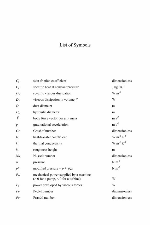
List of Symbols
Cf skin-friction coefficient dimensionless
Cp specific heat at constant pressure J kg-1 K-1
D specific viscous dissipation W m-3
D viscous dissipation in volume V W
D duct diameter m
Dh hydraulic diameter m
F body force vector per unit mass m s-2
g gravitational acceleration m s-2
Gr Grashof number dimensionless
h heat-transfer coefficient W m-2 K-1
k thermal conductivity W m-1 K-1
ks roughness height m
Nu Nusselt number dimensionless
p pressure N m-2
p* modified pressure = p + gz N m-2
Pm mechanical power supplied by a machine (> 0 for a pump, < 0 for a turbine) W
Pf power developed by viscous forces W
Pe Peclet number dimensionless
Pr Prandtl number dimensionless
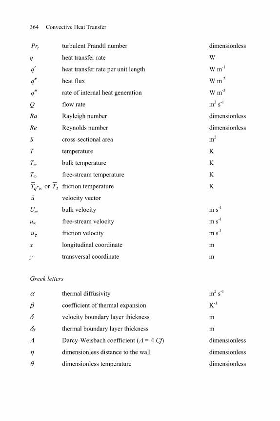
364 Convective Heat Transfer
Prt turbulent Prandtl number dimensionless
q heat transfer rate W
q heat transfer rate per unit length W m-1
q heat flux W m-2
q rate of internal heat generation W m-3
Q flow rate m3 s-1
Ra Rayleigh number dimensionless
Re Reynolds number dimensionless
S cross-sectional area m2
T temperature K
Tm bulk temperature K
T free-stream temperature K
T q w or T friction temperature K
u velocity vector
Um bulk velocity m s-1
u free-stream velocity m s-1
u friction velocity m s-1
x longitudinal coordinate m
y transversal coordinate m
Greek letters
thermal diffusivity m2 s-1
coefficient of thermal expansion K-1
velocity boundary layer thickness m
T thermal boundary layer thickness m
Darcy-Weisbach coefficient ( = 4 Cf) dimensionless
dimensionless distance to the wall dimensionless
dimensionless temperature dimensionless
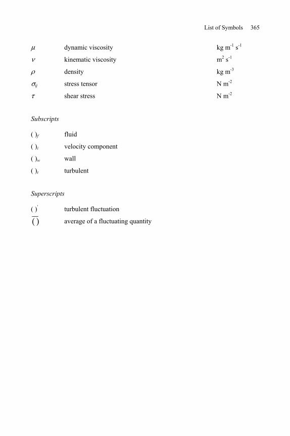
List of Symbols 365
dynamic viscosity kg m-1 s-1
kinematic viscosity m2 s-1
density kg m-3
ij stress tensor N m-2
shear stress N m-2
Subscripts
( )f fluid
( )i velocity component
( )w wall
( )t turbulent
Superscripts
( )' turbulent fluctuation
average of a fluctuating quantity

This page intentionally left blank
References
[ARP 84] V.S. ARPACI and P.S. LARSEN, Convection Heat Transfer, Prentice Hall, Inc., Englewood Cliffs, New Jersey, 1984.
BEJ 95 A. BEJAN, Convection Heat Transfer, 2nd ed., John Wiley & Sons, New York, 1995.
[BER 80] R.F. BERGHOLZ, “Natural convection of a heat generating fluid in a closed cavity”, J. Heat Transfer, vol. 102, 242-247, 1980.
[BIA 04] A.M. BIANCHI, Y. FAUTRELLE and J. ETAY, Transferts thermiques, Presses polytechniques et universitaires romandes, Lausanne, 2004.
BRU 95 H.H. BRUUN, Hot-wire Anemometry, Principles and Signal Analysis, Oxford University Press, Oxford, 1995.
BUR 83 L.C. BURMEISTER, Convective Heat Transfer, John Wiley & Sons, New York, 1983.
[CEB 73] T. CEBECI, “A model for eddy conductivity and turbulent Prandtl number”, J. Heat Transfer, vol. 95, 227, 1973.
CEB 88 T. CEBECI and P. BRADSHAW, Physical and Computational Aspects of Convective Heat Transfer, Springer-Verlag, New York, 1988.
CHA 00 P. CHASSAING, Mécanique des fluides : éléments d’un premier parcours, Cépaduès, Toulouse, 2000.
CHU 72 S.W. CHURCHILL and R. USAGI, “A general expression for the correlation of rates of transfer and other phenomena”, A.I.Ch.E. J., vol. 18, 1121-1128, 1972.
[CHU 75] S.W. CHURCHILL and H.H.S. CHU, “Correlating equations for laminar and turbulent free convection from a vertical surface”, Int. J. Heat Transfer, vol. 18, 1323-1329, 1975.
[CHU 77a] S.W. CHURCHILL and M. BERNSTEIN, “A correlating equation for forced convection from gases and liquids to a circular cylinder in crossflow”, J. Heat Transfer, vol. 99, 300-306, 1977.
[CHU 77b] S.W. CHURCHILL, “A comprehensive correlation equation for laminar, assisting, forced and free convection”, AIChE J., vol. 23, 10-16, 1977.
368 Convective Heat Transfer
[COL 56] D.E. COLES, “The law of the wake in the turbulent boundary layer”, J. Fluid Mech., vol. 1, 191-226, 1956.
[COL 59] D.C. COLLIS and M.J. WILLIAMS, “Two-dimensional convection from heated wires at low Reynolds numbers”, J. Fluid Mech., vol. 6, 357-384, 1959.
[DOC 06] O. DOCHE, Contrôle actif dual des écoulements turbulents pariétaux ; expériences et simulations numériques directes, Phd Thesis, Joseph Fourier University, Grenoble, 2006.
[DRA 81] P.G. DRAZIN and W. REID, Hydrodynamic Stability, Cambridge University Press, 1981.
ECK 72 E.R.G. ECKERT and R.M. DRAKE JR, Analysis of Heat and Mass Transfer, McGraw- Hill, Tokyo, 1972.
EDE 67 A.J. EDE, “Advances in free convection”, Advances in Heat Transfer, vol. 4, 1-64, Academic, New York, 1967.
[FIS 50] M. FISHENDEN and O.A. SAUNDERS, An Introduction to Heat Transfer, Oxford University Press, London, 1950.
FUJ 76 T. FUJII and M. FUJII, “The dependence of local Nusselt number on Prandtl number in the case of free convection along a vertical surface with uniform heat flux”, Int. J. of Heat and Mass Transfer, vol. 19, 121-122, 1976.
[FUK 02] K. FUKAGATA, K. IWAMOTO and N. KASAGI, “Contribution of Reynolds stress distribution to the skin friction in wall-bounded flows”, Phys Fluids, vol. 14, L73-L76, 2002.
[FUK 05] K. FUKAGATA, K. IWAMOTO and N. KASAGI, “Novel turbulence control strategy for simultaneously achieving friction drag and heat transfer augmentation”, Proc. Int. Symp. Turbulence and Shear Flow Phenomena, Williamsburg, Virginia, 27-29 June 2005, 307-312.
GEB 71 B. GEBHART, Heat Transfer, McGraw-Hill, New York, 1971.
[GOL 60] R.J. GOLDSTEIN and E.R.G. ECKERT, “The steady and transient free convection boundary layer on a uniformly heated vertical plate”, Int. J. Heat Mass Transfer, vol. 1, 208-210, 1960.
GUY 91 E. GUYON, J.P. HULIN and L. PETIT, Hydrodynamique physique, Inter-Editions & Editions du CNRS, Paris, 1991.
HAR 98 S. HARMAND, F. MONNOYER, B. WATEL and B. DESMET, “Echanges convectifs locaux sur une couronne d’un disque en rotation”, Rev. Gén. Thermique, vol. 37, 885-897, 1998.
HIN 75 J.O. HINZE, Turbulence: An Introduction to its Mechanism and Theory, McGraw-Hill, New York, 1975.
[HOU 06] T. HOURA and Y. NAGANO, “Effects of adverse pressure gradient on heat transfer mechanism in thermal boundary layer”, Int. J. Heat and Fluid Flow, vol. 27, 967-976, 2006.
References 369
HUE 90 J. HUETZ and J.P. PETIT, “Notions de transfert thermique par convection, traité Génie Energétique”, Techniques de l’Ingénieur, vol. 1, A1540, 1990.
INC 96 F.P. INCROPERA and D.P. DE WITT, Fundamentals of Heat and Mass Transfer, 4th ed., John Wiley & Sons, New York, 1996.
JAC 93 A.M. JACOBI, “A scale analysis approach to the correlation of continuous moving sheet (backward boundary layer) forced convective heat transfer”, J. Heat Transfer, vol. 115, 1058-1061, 1993.
[JIM 04] J. JIMÉNEZ, “Turbulent flows over rough walls”, Annual Review of Fluid Mechanics, vol. 36, 173-196, 2004.
[KAD 81] B.A. KADER, “Temperature and concentration profiles in fully turbulent boundary layers”, Int J Heat Mass Transfer, vol. 24, 1541-1544, 1981.
[KAW 98] H. KAWAMURA, K. OHSAKA, H. ABE and K. YAMAMOTO, “DNS of turbulent heat transfer in channel flow with low to medium-high Prandtl number fluid”, Int. J. Heat and Fluid Flow, vol. 19, 482-491, 1998.
[KAW 04] H. KAWAMURA, H. ABE and Y. MATSU, “Very large-scale structures observed in DNS of turbulent channel flow with passive scalar transport”, 15th Australasian Fluid Mechanics Conference, The University of Sydney, Australia, 13-17 December 2004.
KHA 05 W.A. KHAN, J.R. CULHAM and M.M. YOVANOVICH, “Fluid flow around and heat transfer from an infinite circular cylinder”, J. of Heat Transfer, vol. 127, 785-790, 2005.
KRE 68 F. KREITH, “Convection heat transfer in rotating systems”, Advances in Heat Transfer, vol. 5, 129-251, Academic Press, New York, 1968.
LIM 92 J.S. LIM, A. BEJAN and J.H. KIM, “The optimal thickness of a wall with convection on one side”, Int. J. of Heat and Mass Transfer, vol. 35, 1673-1679, 1992.
LUI 74 A.V. LUIKOV, “Conjugate convective heat transfer problems”, Int. J. of Heat and Mass Transfer, vol. 17, 257-265, 1974.
[MAN 88] N.N. MANSOUR, J. KIM and P. MOIN, “Reynolds -stress and dissipation-rate budgets in a turbulent channel flow”, J. Fluid Mech., vol. 194, 15-44, 1988.
[MEL 05] B. MELISSARI and S.A. ARGYROPOULOS, “Development of a heat transfer dimensionless correlation for spheres immersed in a wide range of Prandtl number uids”, Int. J. of Heat and Mass Transfer, vol. 48, 4333-4341, 2005.
NAK 04 H. NAKAMURA and T. IGARASHI, “Variation of Nusselt number with flow regimes behind a circular cylinder for Reynolds numbers from 70 to 30,000”, Int. J. of Heat and Mass Transfer, vol. 47, 5169-5173, 2004.
NIE 04 D.A. NIELD, “Forced convection in a parallel plate channel with asymmetric heating”, Int. J. of Heat and Mass Transfer, vol. 47, 5609-5612, 2004.
[ORL 00] P. ORLANDI, Fluid Flow Phenomena: A Numerical Toolkit, Kluwer Academy Publishers, 2000.
[PAN 03] A. PANTOKRATORAS, “A note on laminar axisymmetric and two-dimensional glycerol plumes”, Applied Math Modelling, vol. 27, 889-897, 2003.
370 Convective Heat Transfer
[RAM 02] C. RAMIREZ, D.B. MURRAY and J.A. FITZPATRICK, “Convective heat transfer of an inclined rectangular plate”, Exp. Heat Transfer, vol. 15, 1-18, 2002.
[REY 74] A.J. REYNOLDS, Turbulent Flow in Engineering, John Wiley & Sons, London, 1974.
[SCH 79] H. SCHLICHTING, Boundary Layer Theory, McGraw-Hill, New York, 1979.
[SHA 78] R.K. SHAH and A.L. LONDON, “Laminar flow forced convection in ducts”, Chapter 6 in Advanced Heat Transfer, Academic Press, New York, 1978.
[SMI 58] A.G. SMITH and D.B. SPALDING, “Heat transfer in a laminar boundary layer with constant fluid properties and constant wall properties”, J. R. Aerosp. Sci., vol. 62, 60-64, 1958.
SPA 61 D.B. SPALDING, “A single formula for the law of the wall”, J. Appl. Mech., vol. 28, 455-457, 1961.
SPA 62 D.B. SPALDING and W.M. PUN, “A review of methods for predicting heat-transfer coefficients for laminar uniform-property boundary layer flows”, Int. J. of Heat and Mass Transfer, vol. 5, 239-250, 1962.
TAI 95 J. TAINE and J.P. PETIT, Transferts thermiques, mécanique des fluides anisothermes, Dunod, Paris, 1995.
[TAR 09] F.S. TARDU, “Simple two-layer model for temperature distribution in the inner part of turbulent boundary layers in adverse pressure gradients”, Int. J. Heat and Mass Transfer, vol. 52, 2914-2917, 2009.
TEN 72 H. TENNEKES and J.L. LUMLEY, A First Course in Turbulence, M.I.T. Press, Cambridge, Mass., London, 1972.
[TOW 76] A.A. TOWNSEND, The Structure of Turbulent Shear Flow, Cambridge University Press, Cambridge, 1976.
VON 21 T. VON KARMAN, “Über laminare und turbulente Reibung”, Z. Angew. Math Mech vol. 1, 233-252, 1921.
[WEB 05] R.L. WEBB, Principles of Enhanced Heat Transfer, John Wiley & Sons, New York, 1994.
[WHI 72] S. WHITAKER, “Forced convection heat transfer correlations for flow in pipes, past flat plates, single cylinders, and flow in packed beds and tube bundles”, AIChE J., vol. 18, 361-371, 1972.
[WHI 91] F.M. WHITE, Viscous Fluid Flow, 2nd ed., McGraw-Hill, New York, 1991.
Index
A-B
Blasius boundary layer, 55, 281 law, 266, 275, 277, 293-296
Boundary conditions, 33, 35, 47, 57-59, 91-97, 146, 147, 191, 192, 207, 209, 212, 239, 240, 252-268, 304, 309, 335-340, 352 Boundary layer, 58, 199, 204
temperature, 68, 84 thermal, 34, 35, 46, 53, 58-110, 119,
131, 132, 282-307, 316 thickness, 129, 130-149, 16-171, 184,
197, 203, 305 velocity, 57
Boussinesq eddy viscosity model, 324 equation, 162, 177, 203, 204 model, 142
Buffer layer, 219, 229, 245-251, 298 Bulk
temperature, 34, 40, 76, 107-112, 231, 238, 239, 240, 241, 271-279
velocity, 32-46, 79, 106, 215, 231-241, 254, 264-278, 354
C-D
Colburn analogy, 266-273, 290, 294 Conductive sublayer, 222-225, 245-251, 300, 311-318 Couette flow, 9-15
Cylinder, 95-105, 120-124, 154, 158, 180 Darcy-Weisbach drag coefficient, 231 Direct numerical simulations, 218-235 Dittus-Boelter correlation, 231 Drag coefficient, 232-240, 287-300, 310, 319, 321 Duct flow, 31-32
E-F
Eddy diffusivity, 217, 222, 232, 252, 253,
300, 305, 316, 329, 334 closure, 216, 221 spalding model, 224 viscosity, 215-223, 244-258, 284,
298-320 Energy budget, 19-28, 38, 95, 106-112, 180, 239-258, 273-277, 327, 341-358 Energy equation, 2, 6, 19, 36-48, 58-73, 84-118, 142, 150, 177, 191, 203, 204, 265, 267, 294, 326-343, 355 integral, 122-133 Enthalpy flow rate, 114 Falkner-Skan flows, 306- 310 Forced convection, 53, 119, 141-160, 189, 192, 210, 272-278 Friction coefficient, 189, 193 Fully developed flow, 264 hydrodynamically, 36 thermally, 36
372 Convective Heat Transfer
G-H
Grashof number, 8, 143, 152, 192, 278 Head loss coefficient, 33, 266 Heat flux, 3-23, 34-49, 58-118, 121-134, 143-149, 164-188, 206, 267, 283-308, 329-347 Heat-transfer coefficient, 7, 34, 45, 58-83, 148-172, 273, 278
average, 123 local, 34, 78, 121 Hydraulic diameter, 31-48, 231-243, 265-278
I-J
Integral method, 50, 62, 114, 122-135, 149, 166-173 Integration of energy equation, 327
K-L
Kolmogorov dissipative scale, 227 Laminar-turbulent transition, 78, 141 Lévêque solution, 107 Logarithmic layer, 245-259, 291
M-N
Mixed convection, 152, 189, 190, 206, 210 Mixing length, 215, 243-247, 301-309, 325 Modified pressure, 2, 33, 142, 196, 271-275 Natural convection, 141-156, 174, 188, 195, 270, 272
in an enclosure, 196, 201 unsteady, 164-169
Navier-Stokes equation, 2, 37, 53, 94, 108, 212-216, 255, 282 Newtonian fluid, 2, 3, 12 Nusselt number, 9, 34-50, 58-103, 121-138, 143-160, 175, 186, 203, 206, 231, 238, 239, 240, 241, 242, 243, 279
O-P
Outer layer, 211-228, 245-254, 281, 285, 319 Overall heat transfer rate, 36, 62, 68, 129 Plume, 176-182, 196, 326 Poiseuille flow, 211-213, 237 Prandtl number, 8, 35, 36, 121, 127, 129, 143, 158-165, 182, 183, 200, 202, 221-227, 249-279 Prandtl-Taylor analogy, 288-300 Pressure gradient, 11, 55-78, 90, 130, 204, 208, 233, 234, 284-318, 324-342 Principle of superposition, 114
Q-R
Rayleigh number, 9, 143-161, 181-186, 198, 199 Reynolds analogy, 286-310
equations, 216, 271, 274, 233, 332, 342, 343
number, 8, 32, 33, 53, 67-84, 119-129, 137, 192, 212-221, 231-236, 266-278
shear stress, 214, 216, 229-238 Rough walls, 231, 233
S-T
Scale analysis, 55, 58, 87, 98, 142, 167, 184, 195
temperature boundary layer, 62 velocity boundary layer, 32, 64, 62
Shear stress, 11, 12, 18, 55-57, 90, 128-130,
161, 214-220, 233-274, 289-313, 330 velocity, 312-316, 215, 224
Similarity solutions, 59-73, 122-129, 146, 292-314, 326-339 Skin-friction, 9-14, 55-65, 266, 290, 294 Stagnation
plane flow, 128, 131 point, 119, 120, 121, 123, 131
Thermal insulation, 199 resistance, 53, 81, 82, 183-185, 200
Index 373
Turbulent channel flow, 220, 227-240, 252-265 heat flux, 229, 267, 283, 341-347 jet, 351 kinetic energy, 229, 255-259 kinetic energy budget, 258 mixing layers, 323 Prandtl number, 221, 223, 245, 252,
265, 287-309, 313, 318, 325, 338-348 viscosity, 265-268, 324-340, 350, 297 wall flux temperature, 215, 260 wall variables, 215-222, 254-262,
284, 304, 310
U-Z
Van Driest relationship, 309 Viscous sublayer, 218-223, 246-250, 273,
290, 298-319 Wake
velocity, 119 function, 226 thermal, 119