Application Methods artificial neural network(Ann) Back propagation structure for Predicting the value Of bed channel roughnes scoefficient

International Refereed Journal of Engineering and Science (IRJES)

ISSN (Online) 2319-183X, (Print) 2319-1821

Volume 4, Issue 6 (June 2015), PP.23-34

www.irjes.com 23 | Page

Application Methods artificial neural network(Ann) Back

propagation structure for Predicting the value Of bed

channel roughnes scoefficient

Wibowo1, Suripin

2, Kodoatie

2, Isdiyana

3

1Student of Doktoral Program on University of Diponegoro,50241Semarang

1Water Resources Engineering Department, University of Tanjungpura, 78115 Pontianak, Indonesia.

2Civil Engineering, University of Diponegoro, 50241Semarang.

3River Balai, Water Resources Research Center, Bali bang the Ministry of Public Works

Abstract:- Forecasting Manning roughness coefficient act out an important role in hydraulic engineering

because it is use full for the design of hydraulic structures, modeling of river hydraulic sand sediment transport.

This paper used of back propagation neural network method for predicting the Manning roughness coefficient.

Data used in the form of experimental results form the bed configuration in a laboratory and secondary data, a

total of 352data.The results using of backpropagationneural network method is optimized and accurate enough

to7-10-1network architecture, namely one input layer with 10 neurons, one hidden layer with 10 neurons and

one output layer with one neuron. Parameters used logsig activation function and function trainer of training,

with a tolerance of error of 0.01; 0.05learning rate and the maximum epochs much as1000.The model that is Q

prediksi = 0,95 Q simulasi +0,0012. With the correlation coefficientof0.980.The resulting MSE valueis0.00000177

and value for NSE of0.597.The training data as well as the value suit ability the curve of 1:1.

Keywords:- Prediction; Roughness Coefficient;Neural Network Back propagation.

I. INTRODUCTION In engineering hydraulics, Manning roughness coefficient is an important parameter in the design of

hydraulic structures, modeling of river hydraulics and sediment transport (Bilgin & Altun, 2008; Greco et al.,

2014; Mirauda & Greco, 2014). Roughness coefficient of resistance applied to open channel flow, which is used

to calculate the velocity and flow rate (Bilgil, 2003; Bahramifar et al., 2013).

The calculating the roughness coefficient of instead be an easy task because of the complexity of the problem of

open channel. As we know that the Manning roughness coefficient roughness coefficient representing the

resistance of flow by applying the flow in the channel. There for eroughness coefficientis also a fundamental

parameter of fluid flow calculations that is still highly demanded in its application (Bilgil &Altun, 2008).

Resistance of flow in alluvial channels with relatively high accuracy is also a concern for the hydraulic

engineer. However, the problem is still unsolved despite numerous investigations over the last few decades

(Yang &Tan, 2008). Among the problems are due to changes in channel form the bed configuration, the aspect

ratio of the depth and width, the influence of the side wall, and the wall shear stress sisnotuni formally

distributed in the three-dimensional shapes due to the presence of the free surface and the secondary current

(Azamathulla et al., 2013; Samandar, 2011; Bilgin & Altun, 2008; Yang &Tan, 2008; Guo & Julien, 2005).

Along with the growing world of digital (computer), some of models have been developed to simulate this

process. Neither the empirical model (black box model), conceptual model (physical process based), the model

continuously (continuous events), lumped models, distribution models and models of single (Setiawan &

Rudiyan to, 2004). These models are formed by a set of mathematical equations that reflect the behavior of the

hydro logical parameters, so the parameters contained in the equation has a physical meaning (Adidarma, et al.,

2004).

The last few years, art official neural networks (ANN) as a form of black box model (black box model),

has been successfully used optimally to model non-linear of input-output relationship in a complex hydro logic

processes and the potential to become one of the decision-making tool promising in hydrology (Dawson and

Wilby, 2001). ANN is a form of artificial intelligence that has the ability to learn from the data and does not

require a long time in the making models (Setiawan & Rudiyan to, 2004).

These models uses mathematical equations of linear and non-linear that do not take into account at all physical

processes, but the most important in this model is the output produced by the actual approach (Adidarma, et al.,

2004). In addition, the ANN was also able to identify the structure and also effective in connecting the input and

output of simulation and forecasting models (Setiawan and Rudiyan to, 2004).

Application Methods artificial neural network (Ann) Back propagation structure for Predicting the value


The ability of Artificial Neural Networks (ANN) in solving complex problems has been demons trated

in various studies, recently, the development of the body in the application of artificial neural net working river

engineering like Karunanithi et al. (1994), Fauzy & Trilita (2005), Cigizoglu (2005), Antenatal. (2006), Bilgil&

Altun (2008), Samandar (2011), Mary (2011), The control of the water level (Alifia et al., 2012), Azamathulla et

al. (2013), and Bahramifar et al. (2013), Model is as irainfallrun off (Doddy & Ardana, 2013), rainfall prediction

in Jakarta(Nugroho et al, 2013).

Therefore, this paper will apply the method of ANN. The purpose of this paper is to use the approach

of artificial neural network (ANN) for calculating the Manning roughness coefficient using data from laboratory

experiments. In the study raised the flow parameter measurements in the laboratory is used for artificial neural

network as input parameters. The value of calculating the roughness coefficient is calculated later Maning used

to estimate the flow in open channel flow.

II. MATERIALS AND METHODS 2.1 Coefficient of Roughness in Open Channels.

Ina lot of literature it is known that velocity offlowin open channels formulation created by the Robert

Manning (1891), as Equation (1)

V =1

nR2/3 S .....................................(1)

Where Vis the average velocity of the cross section, Nis Manning resistance co efficient, Ris the hydraulic

radius and Sis the hydraulic slope. This formula is derived from semi-empirical that has been used hydraulic

experts during the 18th century.

Dischargeormagnitude of the flow of the river/canal is flowing through the volume flow through ariver cross

section/channel per unit time (Chow, 1959; Soewar no, 1995). Usually expressed in units of cubic meters per

second (m3 / s) orlitersper second (l /sec). Flowis the movement of water in the river channel/channels.

Basically discharge measure mentis a measurement of wet cross-sectional area, the flow rate and water level.

The general formula is used as Equation (2).

Q = V. A ..........................................(2)

Today, Manning equation is more often used as a formulation in hydraulic engineering and expressed respective

lyin Equation (3).

n =1

VR2/3 S .................................(3)

Formulation development at Manning formula also applied to the linear separation method. This linear

separation method has been widely recognized by experts as a hydraulic principles and approaches on the sum

of components resistance. Resistance to the flow in the channel digolongan into 2 (two) types, the first friction

surface (skin friction) that is generated by the boundary surface resistance and depending on the depth of the

flow relative to the size of the elements on the surface roughness limit, both opposition form (form resistance) or

form drag namely roughness related to the geometry of the surface roughness of granules and barrier forms

associated with the basic configuration that govern vortex and secondary circulation. This principle has been

developed in a natural resistance component with rigid base and a natural resistance component with a flexible

base (Meyer-Peter & Muller, 1948; Einstein and Barbarossa, 1952; England, 1966; Smith & McLean, 1977;

Griffiths, 1989; Yang & Tan 2008).

Manning equation formulation in linear separation method as Equation (4).

𝑛 = 𝑛𝑤 + 𝑛′ + 𝑛′′ ……………….(4)

Where𝑛𝑤 isroughness coefficientdue tothe sidewall, with𝑛𝑤 = 𝑅1/6

𝑔 𝑢∗𝑤

𝑈 and𝑢∗𝑤 = 𝜏𝑤 /𝜌. 𝑛′is the resistance

due to friction surfaces(skin friction) or the roughness of granules, the formulan𝑛 ′

𝑅1/6 𝑔 = 𝜏0

′

𝜌

𝑈=

𝑢∗′

𝑈and𝑛′′ is

the resistance that is due to form drag(form drag) orroughnessshape, with the formulation ofn with 𝑛 ′′

𝑅1/6 𝑔 =

𝑢∗

′′

𝑈. Equation (3) on a restated as a function of dimension lesssymbolonan open channel roughness

coefficient(𝑛 ′′

𝑛 ′)as in Equation(5).

𝑛 ′′

𝑛 ′= 𝑓 (𝑅𝑒 , 𝐾𝑟 , 𝜂, 𝑆, 𝐹𝑟 , 𝜎,

𝑏

𝑕) ................(5)

Where 𝑅𝑒 is the Reynolds number, 𝐾𝑟 is relative roughness usually expressed as𝑘𝑠/𝑅 where𝑘𝑠isequivalentwallsurface roughness, ηis across-sectional geometries, S is channels lope, 𝐹𝑟 is the

Froude number and σ is the gradation grain. In the Equation (5) are further tested from the description of the

mechanism and limit the flow channel by Yen (2002&1992). Symbol function in Equation (5) is not linear and



complex. For the sake of simplification made in the conventional approach. As noted, the problem of flow in

open channels may be completed with an error limit of ± 10% (Bilgil, 1998).

These indications show the new and accurate methods are still needed. The existence of the methods that have

high accuracy will reduce error rates. At the ends of the artificial neural network approach to the efficiency of

the pre-assessment approach to predict the roughness coefficient through the use of Artificial Neural Network

(ANN).

2.2 Artificial Neural Network (ANN).

Neural Network (NN) is a learning method that is inspired by the biological network learning system

that occurs on the network of nerve cells (neurons) are connected with one another. NN structure used is Back

propagation (BP) which is a systematic method for training multiplayer. This method has a powerful

mathematical basis, objective and this algorithm to get the form of equation and the coefficient in the formula by

minimizing the number of error squared error by the model developed in the training set (Bilgil & Altun, 2008).

2.3 Algorithm a Back propagation (BP)

Back propagation algorithm on neural network (BPPN) is a systematic approach to training

(calibration) on multi layer percept on neural networks or multilayer (multilayer perceptrons). Layer (layer) The

first consists of a set of inputs and the final layer is the output (target). Among the input layer and output layer

there is a layer in the middle, which is also known as hidden layers (hidden layers), could be one, two, three and

so on. In practice, the number of hidden layers is at most three layers. Input layer mere present asking input

variables, hidden layer represents non linearity(non-linearity) of the network system while the output layer

contains variable output, the last layer output from the hidden layer directly used as the output of the neural

network.

BP training process requires three stages of data input for training feed forward, back propagation to the value of

the error (the error) as well as the adjustment of the weight values of each node of each layer on ANN.

Beginning with feed forward value input, each input to the unit-i(xi) receiving an input signal which will then be

transmitted to the hidden layerz1, ..., zp. Furthermore, the j-the hidden unit will calculate the value of the signal

(zj), which will be tram smitted to the output layer, using the activation function (f)

In simple terms of BPNN described as follows, an input pattern in corporate into the network system to produce

output, which is the compared with the actual output pattern. If there is no difference between the output of the

system and the actual network, then the learning is not necessary. In other words, a weight that indicates the

contribution of input node to hidden nodes, as well as from hidden node to output, in which case the difference

(error) between the output of the system with the actual network, then the weights repaired one backwards, from

the output passes the rough hidden node andr e-input node. Mathematically can be described in the back

propagation algorithm in Equation(6).

𝑧𝑖𝑛 𝑗= 𝑣0𝑗 + 𝑥𝑖𝑣𝑖𝑗

𝑛𝑖=1 ...........................(6)

where 𝑧𝑖𝑛 𝑗 is aktifivasifunctionto calculate thevalue ofthe outputsignalin thehidden nodej; 𝑥𝑖 isthe valueinthe

inputnode ; 𝑣𝑖𝑗 = is theweight valuethat connects theinputnode iwith ahiddennotej. ; 𝑣0𝑗 is

avaluebiaswhichconnects thebiasnode1with thehidden nodej.nisthe number of inputnodesin the inputlayer.

And the output signal from the hidden node j given sigmoid activation function as Equation(7)

𝑧𝑖 = 𝑓(𝑧𝑖𝑛 𝑗) =

1

1+𝑒− 𝑧𝑖𝑛 𝑗

...........................(7)

where𝑧𝑖 isthe signaloutputofhidden nodej. While each unit of output k(Yin),as Equation(8)

𝑌−𝑖𝑛 = 𝑤0𝑗 + 𝑧𝑗𝑤𝑗𝑘𝑝𝑗=1 ...........................(8)

And the activation function to calculate the value of the output signal, as Equation(9)

𝑌 = 𝑓(𝑌−𝑖𝑛) =1

1+𝑒−𝑌−𝑖𝑛 .............................(9)

During the training process progresses, each unit of output compares the target value. for a given input pattern

for calculating the value of the parameters that would improve(update) the weight of the value of each unit in

each layer(Hertz et al., 1991). Nodes in the output layer have a valuebetween0-1.

2.4 Artificial Neural Network (ANN) in Determining a Bed Roughness Coefficient.

In this paper, the calculation of roughness coefficient in open channels is performed using Multilayered

Perception (MLP) artificial neural network. In the literature more likely to use the MLP learning algorithms to

back propagation algorithm Rumelhart et al. (1986). In this algorithm optimization of weights during the

learning process that can use the latest formulation weight given as the output function (level of movement) of

the brain (neurons).



2.5 Performance Model.

Performance models used to measure the accuracy of the model. In this paper, the performance of the model is

used to determine the degree of correspondence between the actual data with the results of forecasting used

measure of correlation coefficient, with the formula in Equation (10).

𝑅 = 𝑥𝑦

𝑥 𝑦 ....................................(10)

Where= 𝑋 − 𝑋 ,𝑋 isthe actualdischarge,𝑋 is the averagevalue ofX, 𝑦 = 𝑌 − 𝑌 , Y is a discharge or as

imulation result of forecasting, 𝑌 , is the average value of the Y value of correlation can be seen in Table.1

Table1. Correlation Coefficient Values

Correlation Coefficient(R2) Iimplication

1 perfect positive

0,6 <R2≤ 1 Good positive direct

0 <R2≤ 0,6 Direct weakly positive

0 There is norrelationship

-0,6 ≤R2< 0 Weak negative direct

-1 ≤R2< -0,6 Negativestraightgood

-1 negative perfect

Source: Soewarno, 1995.

The media n square error (mean square error, MSE). MSE is a measure of the accuracy of the model by

squaring the error for each point of data in a data set and the no btain the average or median value of the sum of

the squares. The formulation of MSE as Equation(11)

𝑀𝑆𝐸 = 𝑦𝑖− 𝑦𝑖 𝑁

𝑖=1

2

𝑁=

𝑒𝑖2𝑁

𝑖=1

𝑁 ...............................(11)

Where 𝑦𝑖 isthe actual valueof data, (𝑦𝑖 ) is the value o f the results of forecasting, Nis the number of data

observations, and𝑒𝑖 is per-point error data. Then used a common procedure error calculating per-point data,

which for the time series followed formulation is: data = pattern + errors for easy, error(error) is written with an

e, the data with the data pattern of X and X. In addition, the sub script i (i =1,2,3, ..., n) are included to show the

data point to-i, so written𝑒𝑖 = 𝑋𝑖 − 𝑋 . If youjustwant to know the magnitude of the error regardless of the

direction it is called absolute error or𝑒𝑖 = 𝑋𝑖 − 𝑋 Another criterion is the accuracy of the model or Nash Sutcliffe Model Efficiency Coefficient (NSE). Nash

gives a good indication for matching of 1:1between simulations and observations. Formulation of Nash as

Equation(12).

𝑁𝑆𝐸 = 1 − 𝑄𝑜𝑏𝑠 −𝑄𝑠𝑖𝑚 2

𝑄𝑜𝑏𝑠 −𝑄 𝑜𝑏𝑠 2 .....................................(12)

WhereQobs areobservational data, Q obs is the averageobservational dataand𝑄𝑠𝑖𝑚 is the value ofthe simulation

results. NSE value criteria can be seen in Table(2).

Table 2 Criteria Value Efficiency Model Nash Sutcliffe Coefficient (NSE).

Nash Sutcliffe Model Efficiency

Coefficient (NSE) Value

Interpretasi

NSE > 0,75 Good

0,36 <NSE 0,75 Ssatisfy

NSE 0,36 Not satisfactory

Source : Motovilov et al., 1999

2.6 Data from Experiment

This paper aims to analyze the performance of artificial neural network back propagation method in

predicting the bottom friction coefficient. Writer wanted to know how the performance of artificial neural

networks back propagation method to recognize patterns of data parameters that‟s lope, depth, grain and flow.

The data used for learning and then to evaluate the use of ANN obtained experiment. The data will be used by

the laboratory results of several researchers and the results of its own research, the data include:

1. DataexperimentalWangandWhite(1993).

2. Data fromexperimentsGuyetal. (1966).

3. Research data fromSisingih(2000).

4. The result ofthe experimentfrom Wibowo(2015)



Table3. Results of Research Data

Parameter Guyetal. (1966). Wibowo(2015) Sisingih(2000) Wang

White(1993).

Slope(S) 0,00015-0,0101 0,006-0,0100 0,007-0,013 0,00001-0,00305

Discharge (Q) (m3/s) 0,028 – 0,643 0,003-0,008 0,003-0,006 0,024-0,410

Ratio (b/h) 2,247-42,105 3,587-9,524 0,667-1,000 3,288-19,335

Velocity(V)

m/s

0,212-1,898 0,132-0,411 0,214-0,429 0,105-1,318

Reynolds Numbers (Re) 2,157-98,753 14,446-50,29 0,003-29,211 4,35-11,42

Froude Numbers (Fr) 0,089-1,714 0,152-0,324 0,194-0,353 0,073-1,049

Fricative

()

0,0015-1,734 0,291-0,842 0,727-1,982 0,021-4,685

Roughness coefficient

(n)

0,010-0,040 0,011-0,026 0,012-0,042 0,015-0,028

Sample 269 40 16 64

2.7Mapping Neural Network in the Roughness Coefficient.

In a study of open channel flow roughness coefficient and the relationship between flow parameters

will be given to the function as Equation (5). 𝑛 ′′

𝑛 ′= 𝑓 (𝑅𝑒 ,

𝑑𝑠

𝑕, 𝑆, 𝐹𝑟 , 𝜎,

𝑏

𝑕, 𝜏∗)

Where 𝑅𝑒 is Reynolds number = 𝑢∗𝑑𝑠/𝜈 , ν is the kinematic viscosity, 𝑑𝑠is granular particles (mm), h is the

average depth, S is the slope of the elongated base channel, 𝐹𝑟 is Frounde number 𝑉𝑟 𝑔𝑕 , 𝑉𝑟 = average speed

of the flow (Q/A), Q is the flow rate, σ is the gradation grain, with𝜎 =1

2 𝑑84

𝑑50+

𝑑50

𝑑16 b is the channel width (m),

𝜏 is the shear stress = ghS, S slope hydraulic, g is the acceleration of gravity and R is radius hydraulic. With

the data in Table (3.1) as a measurement parameter input (input) and output (output) is written in pairs on a set

of data created. This data set is used to calculate the roughness coefficients using Manning formula. For learning

in artificial neural network, the parameters on the right side of the symbol Equation (2.5) is given as input and

roughness coefficient as a target parameter. In the learning process half of the data set used for artificial neural

network learning, the time remaining is used to evaluate the implementation of the artificial neural network

learning.

Input data consists of relative roughness(𝑋1), Reynolds number(𝑋2), Slope(𝑋3),the Froude number(𝑋4),

gradation grain (𝑋5), the depth-width ratio(𝑋6)andshear stress(𝑋7).

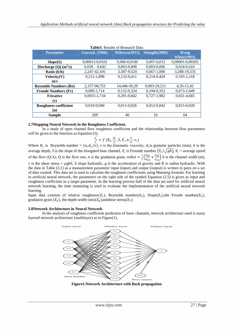
2.8Network Architecture in Neural Network

In the analysis of roughness coefficient prediction of basic channels, network architecture used is many

layered network architecture (multilayer) as in Figure(1).

Figure1.Network Architecture with Back propagation



Specification: X is input nodes in the input layer; Z is hidden node (hidden layer); Y is the output node in the

output layer; 𝑉1,1,…,𝑉𝑛 isthe weightofthe inputlayerto thehidden; 𝑊1,1,…,𝑊𝑛 is the weight of the hidden layer to

the output ; 𝑏𝑣isbiasfromthe inputlayerto thehiddenlayer; 𝑏𝑤 isbiasof thehiddenlayertothe output layer.

2.9Training Process

The training process was conducted on the data as input parameters of network nodes ;

Toleransi error = 0,01; Learning Rate (α) = 0,5; number of iterations = 1000 times

III. RESULTS AND DISCUSSIONS. 3.1 Experiment Results

Determination parameters of the neural network is done by searching for the best value of the hidden neurons

are used. Furthermore, to facilitate the calculation of the iteration process and running experiment data, then use

the software MATLAB. Here are the results of the experiments have been conducted to determine the number of

neurons in the hidden layer Table(4).

Table 4. Comparison of Results of Experiments on Bed Relative Value Roughness Coefficient (n '/ n')

Running Arsitektur

Jaringan

Function

Activation

MSE Correlation

Coefficient

1 7-10-1 logsig 0,0102 0,908

2 7-9-1 logsig 0,0188 0,928

3 7-8-1 logsig 0,0292 0,920

4 7-7-1 logsig 0,0295 0,911

5 7-6-1 logsig 0,0566 0,909

6 7-5-1 logsig 0,0202 0,915

7 7-4-1 logsig 0,0360 0,916

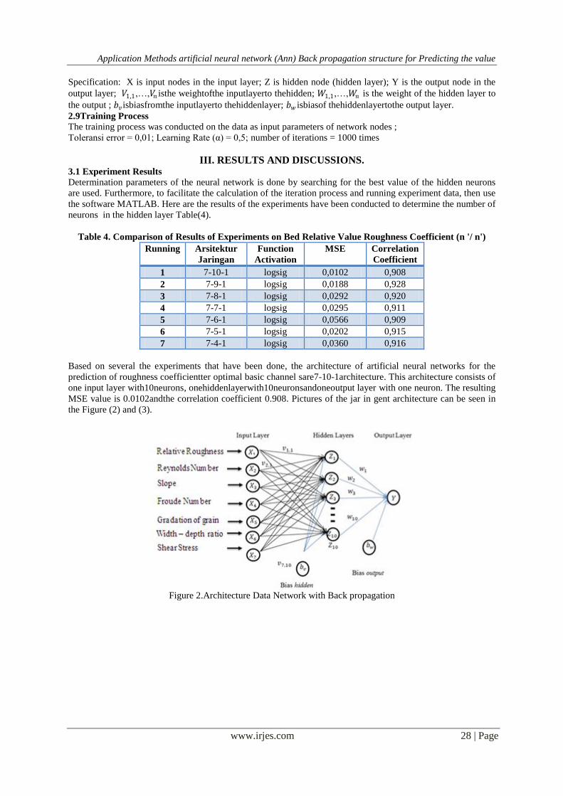
Based on several the experiments that have been done, the architecture of artificial neural networks for the

prediction of roughness coefficientter optimal basic channel sare7-10-1architecture. This architecture consists of

one input layer with10neurons, onehiddenlayerwith10neuronsandoneoutput layer with one neuron. The resulting

MSE value is 0.0102andthe correlation coefficient 0.908. Pictures of the jar in gent architecture can be seen in

the Figure (2) and (3).

Figure 2.Architecture Data Network with Back propagation



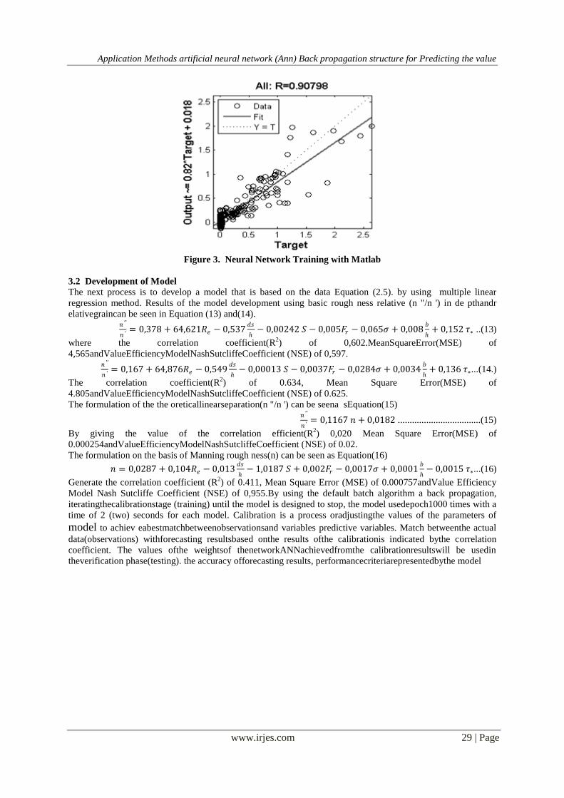
Figure 3. Neural Network Training with Matlab

3.2 Development of Model

The next process is to develop a model that is based on the data Equation (2.5). by using multiple linear

regression method. Results of the model development using basic rough ness relative (n "/n ') in de pthandr

elativegraincan be seen in Equation (13) and(14). 𝑛 ′′

𝑛 ′= 0,378 + 64,621𝑅𝑒 − 0,537

𝑑𝑠

𝑕− 0,00242 𝑆 − 0,005𝐹𝑟 − 0,065𝜎 + 0,008

𝑏

𝑕+ 0,152 𝜏∗ ..(13)

where the correlation coefficient(R2) of 0,602.MeanSquareError(MSE) of

4,565andValueEfficiencyModelNashSutcliffeCoefficient (NSE) of 0,597. 𝑛 ′′

𝑛 ′= 0,167 + 64,876𝑅𝑒 − 0,549

𝑑𝑠

𝑕− 0,00013 𝑆 − 0,0037𝐹𝑟 − 0,0284𝜎 + 0,0034

𝑏

𝑕+ 0,136 𝜏∗...(14.)

The correlation coefficient(R2) of 0.634, Mean Square Error(MSE) of

4.805andValueEfficiencyModelNashSutcliffeCoefficient (NSE) of 0.625.

The formulation of the the oreticallinearseparation(n "/n ') can be seena sEquation(15) 𝑛 ′′

𝑛 ′= 0,1167 𝑛 + 0,0182 ...................................(15)

By giving the value of the correlation efficient(R2) 0,020 Mean Square Error(MSE) of

0.000254andValueEfficiencyModelNashSutcliffeCoefficient (NSE) of 0.02.

The formulation on the basis of Manning rough ness(n) can be seen as Equation(16)

𝑛 = 0,0287 + 0,104𝑅𝑒 − 0,013𝑑𝑠

𝑕− 1,0187 𝑆 + 0,002𝐹𝑟 − 0,0017𝜎 + 0,0001

𝑏

𝑕− 0,0015 𝜏∗...(16)

Generate the correlation coefficient (R2) of 0.411, Mean Square Error (MSE) of 0.000757andValue Efficiency

Model Nash Sutcliffe Coefficient (NSE) of 0,955.By using the default batch algorithm a back propagation,

iteratingthecalibrationstage (training) until the model is designed to stop, the model usedepoch1000 times with a

time of 2 (two) seconds for each model. Calibration is a process oradjustingthe values of the parameters of

model to achiev eabestmatchbetweenobservationsand variables predictive variables. Match betweenthe actual

data(observations) withforecasting resultsbased onthe results ofthe calibrationis indicated bythe correlation

coefficient. The values ofthe weightsof thenetworkANNachievedfromthe calibrationresultswill be usedin

theverification phase(testing). the accuracy offorecasting results, performancecriteriarepresentedbythe model



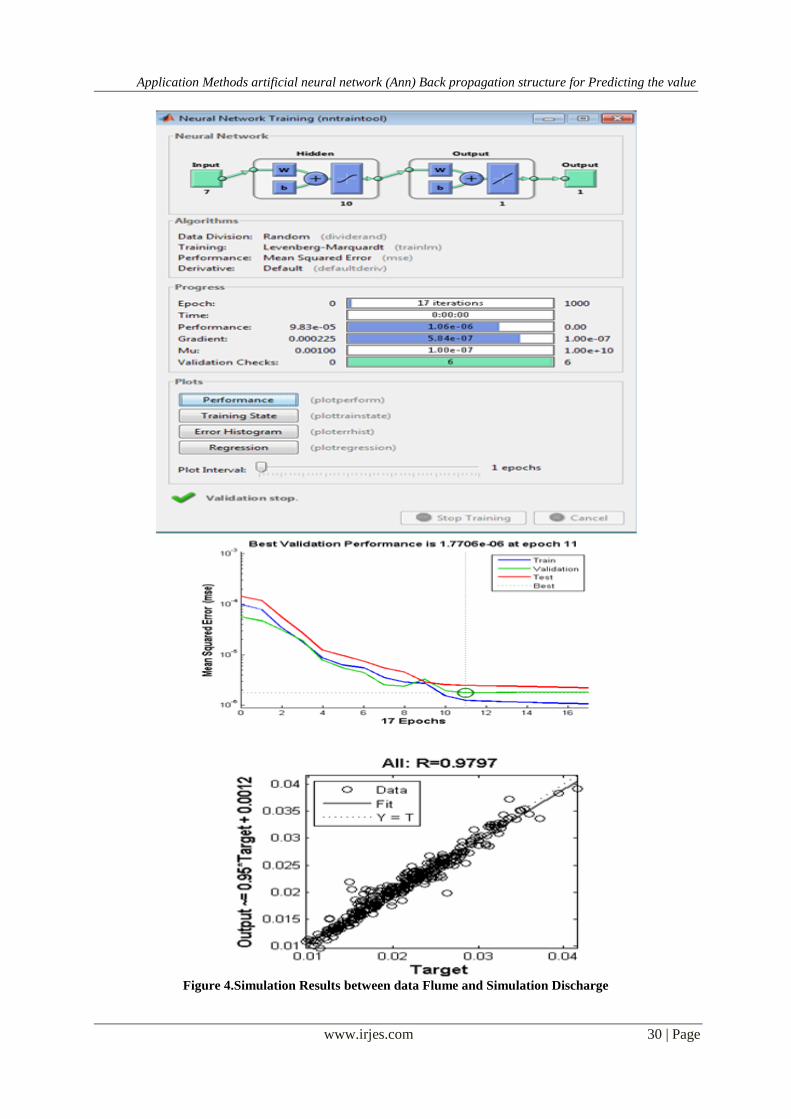
Figure 4.Simulation Results between data Flume and Simulation Discharge



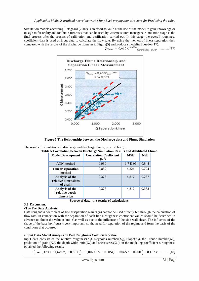
Simulation models according Refsgaard (2000) is an effort to valid at the use of the model to gain knowledge or

in sigh to far reality and too btain forecasts that can be used by waterre source managers. Simulation stage is the

final process after the process of calibration and verification carried out. In this stage, the overall roughness

coefficient data is used as input data to calculate the flow rate. By using the method of linear separation then

compared with the results of the discharge flume as in Figure(5) andproducea modelin Equation(17).

𝑄𝑓𝑙𝑢𝑚𝑒 = 0,436 𝑄0,8834𝑆𝑒𝑝𝑎𝑟𝑎𝑡𝑖𝑜𝑛 𝑙𝑖𝑛𝑒𝑎𝑟 .............(17)

Figure 5 The Relationship between the Discharge data and Flume Simulation

The results of simulations of discharge and discharge flume, asin Table (5).

Table 5 Correlation between Discharge Simulation Results and debilitated Flume.

Model Development Correlation Coefficient

(R2)

MSE NSE

ANN method 0,980 1,7 E-06 0,844

Linear separation

method

0,859 4,324 0,774

Analysis of the

relative dimensions

of grain

0,378 4,817 0,287

Analysis of the

relative depth

dimension

0,377 4,817 0,388

Source of data: the results of calculations.

3.3 Discussion.

•The Pre Data Analysis.

Data roughness coefficient of line arseparation results (n) cannot be used directly but through the calculation of

flow rate. In connection with the separation of each line a roughness coefficient values should be described in

advance to obtain the value n 'and n"as well as due to the influence of the side wall shear. The influence of the

shape of the base konfiguasri very important, so the need for separation of the regime and form the basis of the

conditions that occurred.

•Input Data Model Analysis on Bed Roughness Coefficient Value

Input data consists of the relative roughness(X1), Reynolds number(X2), Slope(X3), the Froude number(X4),

gradation of grain (X5), the depth-width ratio(X6) and shear stress(X7) on the modeling coefficient s roughness

obtained the following results 𝑛 ′′

𝑛 ′= 0,378 + 64,621𝑅𝑒 − 0,537

𝑑𝑠

𝑕− 0,00242 𝑆 − 0,005𝐹𝑟 − 0,065𝜎 + 0,008

𝑏

𝑕+ 0,152 𝜏∗ ............(18)



With a correlation coefficient (R2) of 0.602(0.6 <R

2 <1) which shows the relationship between input variables

(independent variables) have a positive direct relationship Good. This means that data is correlated. Mean

Square Error (MSE) amounted to4.565% (<5%). Error below 5% indicates that the error between the actual

model and simulation is below to lerance. ValueEfficiencyModelNashSutcliffeCoefficient (NSE) of 0,597(0,36

<NSE 0,75) which shows that the interpretation between actual and simulated models in satisfactory

condition, or can be correlated with Good. Similarly, also by using the relative depth. Thus, the data input can

be used on the production model of the channel bottom friction coefficient.

•Separation of Linear Model Analysis on the Bed Roughness Coefficient Value.

The model obtained in the the oreticallinearseparation method(n "/n ') can be seenas Equation(19). 𝑛 ′′

𝑛 ′= 0,1167 𝑛 + 0,0182 ...................(19)

By giving the value of the correlation coefficient(R2) 0,020(0 <R

2 <0.6) which shows the relationship

between input variables (independent variables) have a direct relationship weakly positive. This means that data

is correlated poorly. Mean Square Error (MSE) of 0,000254(<5%). Error below 5% indicates that the error

between the actual model and simulation is below to lerance and very Good.

ValueEfficiencyModelNashSutcliffeCoefficient (NSE) of 0,02(NSE <0.36) which shows that the interpretation

of the actual model and simulation in less than satisfactory condition or less correlated is good.

• Analysis on the Model Manning the Bed Roughness Coefficient Value

The model formulation Manning invitation dimensional analysis(n) can be seen as Equation(20)

𝑛 = 0,0287 + 0,104𝑅𝑒 − 0,013𝑑𝑠

𝑕− 1,0187 𝑆 + 0,002𝐹𝑟 − 0,0017𝜎 + 0,0001

𝑏

𝑕− 0,0015 𝜏∗ ...............(20)

By giving the value of the correlation coefficient (R2) 0.411(0 <R

2<0.6) which shows the relationship between

input variables (independent variables) have a direct relationship weakly positive. This means that data is

correlated poorly. Mean Square Error (MSE) of 0,000757(<5%). Error below 5% indicates that the error

between the actual model and simulation is below to lerance and very good. Value Efficiency Model Nash

Sutcliffe Coefficient (NSE) of 0,955(NSE>0.75) which shows that the interpretation of the actual model and the

simulation under condition scorrelate well.

•Analysis on Manning on Flow Model.

Based on the Table(4.2) obtained results for the model artificial neural network(ANN) have satisfactory

results, whether of the correlation between the variablesof0,980(0,6 <R2<1) which shows the relationship

between input variables (independent variables) have a relationship strong positive immediately. This means

that the data correlates very well. Mean Square Error (MSE) of 0,00000177(<5%).

Error below 5% indicates that the error between the actual model and simulation is below to lerance

and shown very good relationship. For the best fore casting method is the method that produces the smallest

error. Value Efficiency Model Nash Sutcliffe Coefficient (NSE) of 0.597(0.36 <NSE 0.75) which shows that

the interpretation between actual and simulated models in satisfactory condition, or can be correlated with

either. Similarly, also by using the relative depth.

Similarly, the flow separation method that shows the results of the correlation between variables in the

model𝑄𝑓𝑙𝑢𝑚𝑒 = 0,436 𝑄𝑠𝑖𝑚𝑢𝑙𝑎𝑠𝑖0,8834

with R2=0,859 (0,6 <R

2< 1) which shows the relationship between input

variables (independent variables) has a direct relationship strong positive. This means that the data correlates

very well. Mean Square Error (MSE) of 0,00000177(<5%). Error below 5% indicates that the error between the

actual model and simulation is below to lerance and devoted relationship very well. For the best fore casting

method is the method that produces the smallest error. Value efficiency model Nash Sutcliffe coefficient (NSE)

of0,774(NSE >0,75) which shows that the interpretation of the actual model and the simulation under condition

scorrelate well.

Whereas the method of analysis dimensions that are less good result.

IV. CONCLUSION Based on the analysis and discussion it can be concluded as follows:

1. Utilization of ANN to the practical application of basic channels for ecastin groughness coefficient

generally reliable.

2. The best results from the model ANN depends on the quality of the data, including in this case the length

of the data so that the model ANN is able to perform pattern recognition in put and output relationship.

3. ANN Back propagationbestregression modelbasedinputwitharchitecture7- 10 -of 1 (7 units of inputto

theinputlayer-10hidden unitsin the hidden layer-1 unitof outputin the output layer) is moreaccuratelyused

inforecastingkoefsienbasicroughnessandprovedmore capablefollowthe characteristicsofthe actual



datawiththe value ofthe correlationbetween variablesat0.980 with modelobtainedthe𝑄𝑝𝑟𝑒𝑑𝑖𝑘𝑠𝑖 =

0,95 𝑄𝑠𝑖𝑚𝑢𝑙𝑎𝑠𝑖 + 0,0012,NSEvaluesof 0.844andMSE of0.00000177.

4. Modellinearseparationcan beused to estimate theflow rateto the conditionsforthe basic shapeof channels.

5. Linearseparation modelcanbe usedto estimatethe flow rate bythe basicconditions oftheirshapeto the shape

ofthe channel𝑄𝑓𝑙𝑢𝑚𝑒 = 0,436 𝑄𝑠𝑖𝑚𝑢𝑙𝑎𝑠𝑖0,8834

with (R2=0.859).

ACKNOWLEDGMENTS

Experimental work carried out in the Central Solo River, Indonesia. The author would like to thank the

Balai of Solo River in Central Java province, which has been providing information and data-the data to support

this research and The author would like to acknowledge the assistance of Surip in, Robert Kodoatie, Isdiyana,

Kirno and Family in conductingex periments too. Special thanks to Uray Nurhayati, Ajeng, Hanif and Amira for

their help during the work.

REFERENCES [1]. Adidarma, W.K., Hadihardaja, I.K., and Legowo, S. (2004). “Rain-Runoff Modelling Comparison

Between Artificial Neural Network(ANN) andNRECA". ITBCivil Engineering Journal, Vol. 11No.3:

105-115

[2]. Alifia, F.A, Triwiyatno, A., and Wahyudi., 2012. “Control System Design of Adaptive Neuro Fuzzy

Inference System (ANFIS) “Case Study: Water Front Pengontoran Altitudeand Temperature Steam

Boiler Steam Drum, transient Journal, Vol.1, No.4, 2012, ISSN: 2302-9927, 312, Semarang.

[3]. Altun H, Bilgil A, Fidan CF. Treatment of multi-dimensional data to enhance neural network

estimators in regression problems. Expert Systems with Applications 2006;32(2):Available online from

http://www.sciencedirect.com/.

[4]. Azamathulla, H. Md., Ahmad Z., and Aminuddin Ab. Ghani, 2013.” An Expert System for Predicting

Manning‟s Roughness Coefficient in Open Channels by Using Gene expression Programming “ Neural

Comput & Applic, 23:1343–1349.

[5]. Bahramifar, A, Shirkhanib,R., and Moham madic, M., 2013. ” An ANFIS-based Approach for

Predicting the Manning Roughness Coefficient in Alluvial Channels at the Bank-full Stage “,IJE

Transactions B: Applications Vol. 26, No. 2, pp.177-186.

[6]. Bilgil, A and Altun, H., 2008. “ Investigation of Flow Resistance in Smooth Open Channels using

Artificial Neural Networks”. Flow Meas Instrum 19:404–408.

[7]. Bilgil, A., 2003. “Effect of Wall Shear Stress Distribution on Manning Coefficient of Smooth Open

Rectangular Channel Flows “,Turkish J. Eng. Env. Sci.27 , pp. 305 – 313.

[8]. BilgilA., 1998.” The Effect of Wall Shear Stress on Friction Factor in Smooth Open Channel Flows,

Ph.D.Thesis.Trabzon (Turkey):Karadeniz Technical University,Turkish.

[9]. Chow, V.T., 1959,” Open Chanel Hydraulics”, Mc Graw Hill Kogakusha, Ltd.

[10]. Cigizoglu HK. “ Application of Generalized Regression Neural Networks to Intermittent Flow

Forecasting and Estimation. Journal of Hydrologic Engineering, 2005,pp.336–341.

[11]. Dawson, C.W. and Wilby, R.L. (2001). “Hydrological Modelling Using Artificial Neural Networks”.

Progress in Physical Geography, 25-1: 80-108.

[12]. Doddy. P., and Ardana. Heka., 2013. “Artificial Network Application Requirements (arificial Neural

Network) In Model isasi Rainfall Runoff with Comparing theTraining Algorithm(Case Study:

DASTukadJOGADING, 139A), the National Conference of Civil Engineering7(context 7), pp.A107-

A114. Elevenuniversitiesin March(UNS) –Surakarta

[13]. Einstein, H A., and Barbarossa, 1952. “ River Channels Rougness .” Trans. ASCE, 117, pp.1121-

1132.

[14]. Engelund, F., 1966." Hydraulic Resistance of Alluvial Streams." J.Hydr.Div.,ASCE, 92 (HY2), 315-

326.

[15]. Fauzi, M and Trilita,M,N., 2005.” Application sarificial Neural Network for Flow Forecasting Aungai

Blega". Jurnal Engineering Planning, Vol1, No.3.UPN Veteran, Jawa Timur.

[16]. Greco, M., Mirauda., D., and Plantamura, V. A., 2014.” Manning‟s Roughness Through the Entropy

Parameter for Steady Open Channel Flows In Low Submergence” 2th International Conference on

Computing and Control for the Water Industry, CCWI2013, ScienceDirect. Procedia Engineering 70

.pp773 –780.

[17]. Griffiths., G. A., 1989. “ Form Resistance In Gravel Channels With Mobile beds “.Journal of

Hydraulic Engineering, Vol. 115, No. 3,© ASCE. Paper No. 23245.pp 340-355.

[18]. Guo, J. and Julien, P.Y., 2005. “Shear Stress in Smooth Rectangular Open-Channel Flows”, Journal of

Hydraulic Engineering,ASCE, Vol. 131 , No. 1,pp. 30–37.



[19]. Hertz, J.; Krogh, A.; Palmer, R. G., 1991. “ Introduction to the Theory of Neural Computation,

Redwood City, CA: Addison Wesley.

[20]. Karunanithi N, Grenney WJ, Whitly D, Bovee K. Noural networks for river flow prediction. Journal of

Computing in Civil Engineering 1994;8. Pp. 201–220.

[21]. Meyer, Peter, and Muller, 1948. “ Formula for Bed-Load Transport ”, Ins.Ass. Hydr.Res. 2nd

Meeting,

Stockholm

[22]. Mirauda, D., Greco, M., and Moscarelli, P., 2011. “ Entropy Based Expeditive Methodology for Rating

Curves Assessment”. Proceedings of the International Conference on Water, Energy and Environment,

Phuket, Thailand, 1351-1356.

[23]. Motovilov, Y.G., Gottschalk, L., Engeland, K. & Rodhe, A. 1999. Validation of a Distributed

Hydrological Model Against Spatial Observations. Elsevier Agricultural and Forest Meteorology. 98,

pp. 257-277.

[24]. Nugroho, J.T., Liong,T.H., Safwan Hadi and Bayong Tjasyono HK., 2013.”

IncreasedMonthlyRainfallPredictionAccuracyinJakartaRegionalDataUsingTropicalRainfallMeasuring

Mission(TRMM) andNetwork-Based DataCosmic RaysTermsArtificial, Journalof Aerospace Sciences,

Vol. 11No.1, pp41-48,Jakarta.

[25]. Refsgaard, J.C. 2000. Towards a Formal Approach to Calibration and Validation of Models Using

Spatial Data, Dalam R. Grayson & G. Blöschl. Spatial Patterns in Catchment Hydrology:

Observations and Modelling. Cambridge University Press, Cambridge, pp. 329 – 354.

[26]. Rumelhart DE, Hinton GE, Williams RJ, 1986. “ Learning internal representation by error propagation.

In: Parallel and distributed processing: Explorations in the microstructure of cognition. Vol 1:

Foundations. Cambridge, MA: MIT Press.

[27]. Samandar. A., 2011.” A Model of Adaptive Neural-Based Fuzzy InferenceSystem (ANFIS) for

Prediction of Friction Coefficient inOpen Channel Flow “, Scientific Research and Essays Vol. 6(5),

pp. 1020-1027.

[28]. Setiawan, B.I., and Rudiyanto. (2004). “ Applicationof NeuralNetworkstoPrediction ofWatershed",

Proceedings ofWorkshopSimulationandComputingTechnologyandApplications2004 -BPPT, Jakarta.

[29]. Soewarno, 1995. “HydrologyApplicationsStatistical MethodsforDataAnalysis, Volume1and2",

PublisherNovaBandung.

[30]. Sisingih, D., 2000, “Relationship Study of Bedform on Hydraulic roughness coefficient on the Open

Channel ", Thesis Master of Civil Engineering, ITB, Bandung.

[31]. Smith, J.D. and McLean, S.R., 1977. “Spatially Averaged Flow Over a Wavy Surface ”. J. Geophys.

Res., 84(12), 1735-1746.

[32]. Wibowo, H., 2015. “ Manning Roughness Coefficient Study on Bed Materials Non-Cohesive with

Parameters Using Entropy to Open Channel Flow”, Proceedings of International Conference : Issues,

Management And Engineering In The Sustainable Development On Delta Areas Semarang, Indonesia

– February 20th, 2015Paper No. XXX (The number assigned by the OpenConf System).

[33]. Wibowo, H., Suripin, Kodoatie, R., and Isdiyana., 2015.” Comparingthe Calculation Method of the

Manning Roughness Coefficientin Open Channels”.Proceedings of International Conference,The 1st

Young Scientist International Conference of Water Resources Development and Environmental

Protection, Malang, Indonesia.

[34]. Yang, S.Q., and Tan, S.K., 2008. “ Flow Resistance over Mobile Bed in an Open-Channel Flow

“,Journal of Hydraulic Engineering, ASCE, Vol. 134,No. 7,pp. 937-947.

[35]. Yanti., N., 2011.” Application of Neural Network Methodwith Back Propagation Structure for Drug

Stock Prediction At Pharmacies (Case Study: Pharmacies ABC), National Seminaron Information

Technology Applications (SNATI 2011) ISSN: 1907-5022, Yogyakarta.

[36]. Yen, B. C., 2002. “ Open Channel Flow Resistance.” Journal of Hydraulic Engineering” , Vol 128(1).

Pp. 20-39.

[37]. Yen, B. C.,1992. „„Dimensionally Homogeneous Manning‟s Formula.‟‟ J.Hydraul. Eng.,118-(9), 1326

–1332; Closure: (1993),.119(12), 1443–1445.

a.