FACULTY OF SCIENCE AND TECHNOLOGY

DEPARTMENT OF PHYSICS AND TECHNOLOGY

The Hotelling-Lawley Trace Statistic forChange Detection in Polarimetric SAR DataUnder the Complex Wishart Distribution

Vahid AkbariStian N. AnfinsenAnthony P. Doulgeris

IGARSS 2013

Overview

• Propose a new test statistic for change detection

• Polarimetric SAR

• MLC covariance Matrix Data

• Assume scaled complex Wishart distribution

• Hotelling-Lawley trace statistic

• Approximated by a Fisher-Snedecor distribution

• Demonstrated as a CFAR detector

• Compared to Conradsen’s Likelihood Ratio Test statistic

1 / 9

Theory

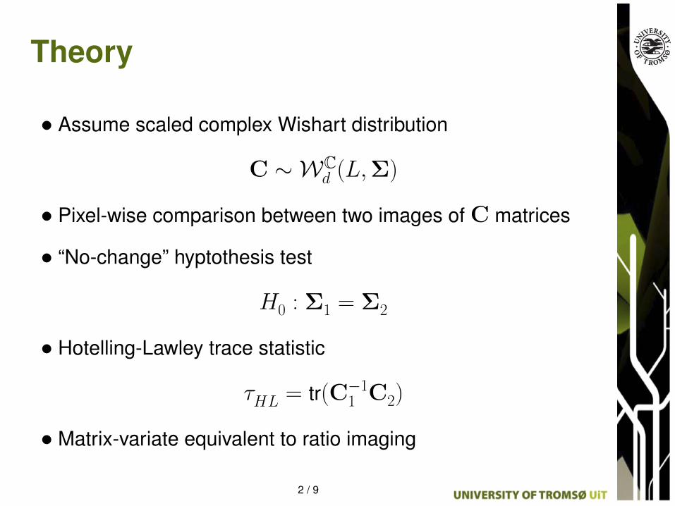
• Assume scaled complex Wishart distribution

C ∼ WCd (L,Σ)

• Pixel-wise comparison between two images of C matrices

• “No-change” hyptothesis test

H0 : Σ1 = Σ2

• Hotelling-Lawley trace statistic

τHL = tr(C−11 C2)

• Matrix-variate equivalent to ratio imaging

2 / 9

Theory

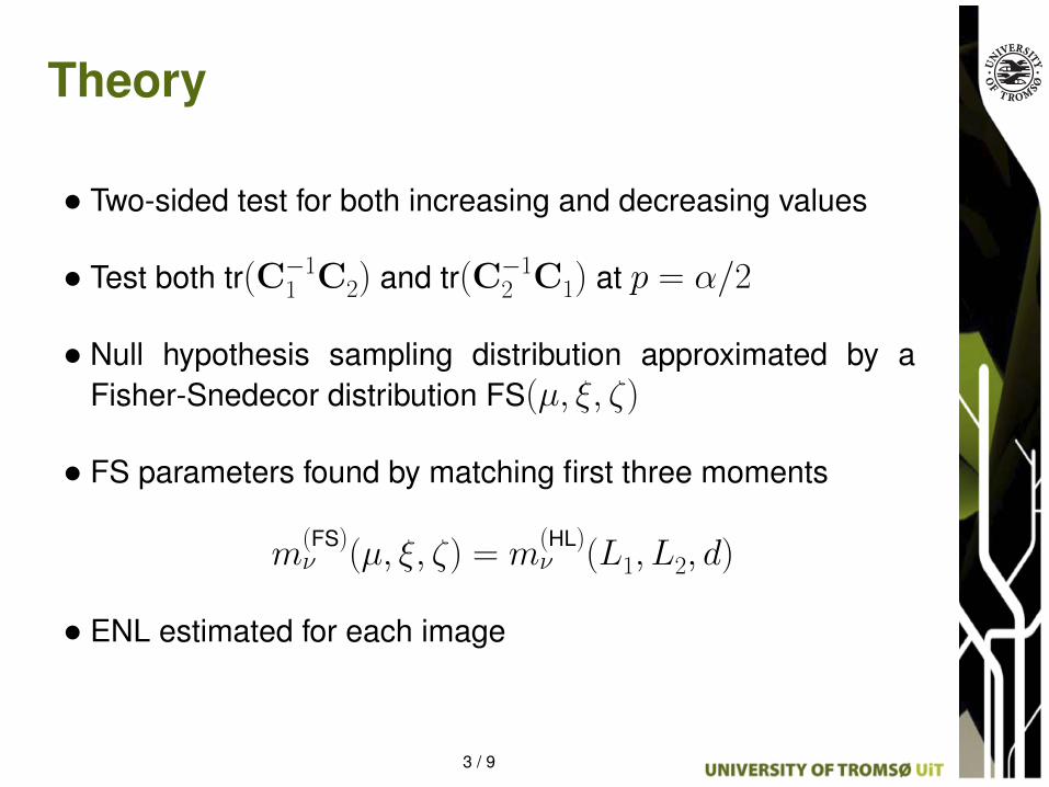
• Two-sided test for both increasing and decreasing values

• Test both tr(C−11 C2) and tr(C−12 C1) at p = α/2

• Null hypothesis sampling distribution approximated by aFisher-Snedecor distribution FS(µ, ξ, ζ)

• FS parameters found by matching first three moments

m(FS)ν (µ, ξ, ζ) = m

(HL)ν (L1, L2, d)

• ENL estimated for each image

3 / 9

Theory

• Compare to Conradsen’s Likelihood Ratio Test statistic• Also known as the Bartlett distance

τLRT = τB = −2ρ logQ

Q =|C1|L1|C2|L2

∣∣∣L1C1+L2C2

L1+L2

∣∣∣L1+L2

ρ = 1− 2d2 − 1

6d

(1

L1

+1

L2− 1

L1 + L2

)

• Sampling distribution is a sum of three χ-squareddistributions

4 / 9

Results - Simulated Pauli Images

12-Looks, Σs from real data, 3 changesBrightness increase, decrease and polarimetric change

(a) test image 1 (b) test image 2 (c) log(⌧HL) (d) log(⌧B)

(e) pdf of ⌧HL (f) pdf of ⌧B (g) HL test detection result (h) Bartlett test detection result

Fig. 1. Comparison of HL test and Bartlett test with data simulated from the complex Wishart model.

and the third-order moment is given as

m(HL)3 = E{⌧3

HL}

=L3

a

Q5a � 5Q3

a + 4Qa⇥

d3

✓(Q2

a � 1) +3Qa

Lb+

4

L2b

◆

+ d2

✓3Qa +

3(Q2a + 2)

Lb+

6Qa

L2b

◆

+ d

✓4 +

6Qa

Lb+

2Q2a

L2b

◆�.

(10)

We seek expressions for the parameters of the FS distri-bution in terms of the distribution parameters of the scaledWishart matrices A and B, i.e., L = La = Lb and d. Thesolutions for µ, ⇠ and ⇣ are defined by the equation system

m(FS)⌫ (⇠, ⇣, µ) = m(HL)

⌫ (L, d) , ⌫ = 1, 2, 3 . (11)

An analytic solution for µ is easily found by matching thefirst-order moments. To match the second and third-ordermoments and retrieve the shape parameters, we use minimumdistance optimization [17] and minimize

✏2 =

3X

⌫=2

(m(HL)⌫ � m(FS)

⌫ )2 . (12)

Estimation of the equivalent number of looks is a critical pointin this procedure. To do this accurately and automatically, weuse the unsupervised method by Anfinsen et al. in [18].

3. RESULTS

We have performed a number of test on simulated and realdata, that will all be presented in a future journal paper. Dueto limited space, we here only show an experiment where wehave generated two test images with eight classes that followa scaled complex Wishart distribution with L = 12 and theirindividual ⌃ computed from samples of real data. The testimages represent times t0 and t1. They are shown in Fig. 1(a) and (b) as Pauli images. Here we see that the changesoccuring are: (i) a transition from class 1 to class 8 along avertical strip centered in the upper half of the images; (ii) atransition from class 5 to class 7 in a vertical strip centeredin the lower half of the images; (iii) the transition from class5 to class 1 in the central square. Test statistic images forthe proposed HL test (⌧HL) and the Bartlett test (⌧B) [3] arerespectively shown in (c) and (d) on logarithmic scale to en-hance the contrast. The histograms of ⌧HL and ⌧B follow in(e) and (f), before the change detection results obtained withthresholds set to obtain a CFAR of 1% are shown in (g) and(h).

A clear difference in the behaviour of the test statistics

����

5 / 9

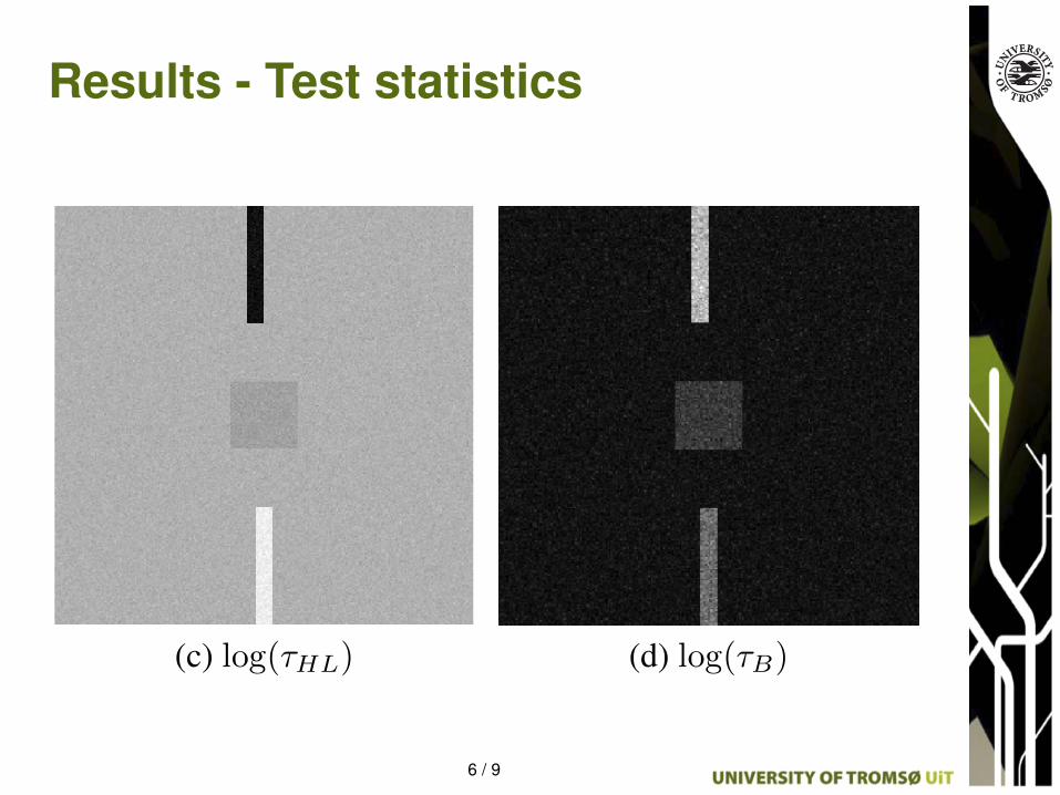
Results - Test statistics

(a) test image 1 (b) test image 2 (c) log(⌧HL) (d) log(⌧B)

(e) pdf of ⌧HL (f) pdf of ⌧B (g) HL test detection result (h) Bartlett test detection result

Fig. 1. Comparison of HL test and Bartlett test with data simulated from the complex Wishart model.

and the third-order moment is given as

m(HL)3 = E{⌧3

HL}

=L3

a

Q5a � 5Q3

a + 4Qa⇥

d3

✓(Q2

a � 1) +3Qa

Lb+

4

L2b

◆

+ d2

✓3Qa +

3(Q2a + 2)

Lb+

6Qa

L2b

◆

+ d

✓4 +

6Qa

Lb+

2Q2a

L2b

◆�.

(10)

We seek expressions for the parameters of the FS distri-bution in terms of the distribution parameters of the scaledWishart matrices A and B, i.e., L = La = Lb and d. Thesolutions for µ, ⇠ and ⇣ are defined by the equation system

m(FS)⌫ (⇠, ⇣, µ) = m(HL)

⌫ (L, d) , ⌫ = 1, 2, 3 . (11)

An analytic solution for µ is easily found by matching thefirst-order moments. To match the second and third-ordermoments and retrieve the shape parameters, we use minimumdistance optimization [17] and minimize

✏2 =

3X

⌫=2

(m(HL)⌫ � m(FS)

⌫ )2 . (12)

Estimation of the equivalent number of looks is a critical pointin this procedure. To do this accurately and automatically, weuse the unsupervised method by Anfinsen et al. in [18].

3. RESULTS

We have performed a number of test on simulated and realdata, that will all be presented in a future journal paper. Dueto limited space, we here only show an experiment where wehave generated two test images with eight classes that followa scaled complex Wishart distribution with L = 12 and theirindividual ⌃ computed from samples of real data. The testimages represent times t0 and t1. They are shown in Fig. 1(a) and (b) as Pauli images. Here we see that the changesoccuring are: (i) a transition from class 1 to class 8 along avertical strip centered in the upper half of the images; (ii) atransition from class 5 to class 7 in a vertical strip centeredin the lower half of the images; (iii) the transition from class5 to class 1 in the central square. Test statistic images forthe proposed HL test (⌧HL) and the Bartlett test (⌧B) [3] arerespectively shown in (c) and (d) on logarithmic scale to en-hance the contrast. The histograms of ⌧HL and ⌧B follow in(e) and (f), before the change detection results obtained withthresholds set to obtain a CFAR of 1% are shown in (g) and(h).

A clear difference in the behaviour of the test statistics

����

6 / 9

Results - Histograms(a) test image 1 (b) test image 2 (c) log(⌧HL) (d) log(⌧B)

(e) pdf of ⌧HL (f) pdf of ⌧B (g) HL test detection result (h) Bartlett test detection result

Fig. 1. Comparison of HL test and Bartlett test with data simulated from the complex Wishart model.

and the third-order moment is given as

m(HL)3 = E{⌧3

HL}

=L3

a

Q5a � 5Q3

a + 4Qa⇥

d3

✓(Q2

a � 1) +3Qa

Lb+

4

L2b

◆

+ d2

✓3Qa +

3(Q2a + 2)

Lb+

6Qa

L2b

◆

+ d

✓4 +

6Qa

Lb+

2Q2a

L2b

◆�.

(10)

We seek expressions for the parameters of the FS distri-bution in terms of the distribution parameters of the scaledWishart matrices A and B, i.e., L = La = Lb and d. Thesolutions for µ, ⇠ and ⇣ are defined by the equation system

m(FS)⌫ (⇠, ⇣, µ) = m(HL)

⌫ (L, d) , ⌫ = 1, 2, 3 . (11)

An analytic solution for µ is easily found by matching thefirst-order moments. To match the second and third-ordermoments and retrieve the shape parameters, we use minimumdistance optimization [17] and minimize

✏2 =

3X

⌫=2

(m(HL)⌫ � m(FS)

⌫ )2 . (12)

Estimation of the equivalent number of looks is a critical pointin this procedure. To do this accurately and automatically, weuse the unsupervised method by Anfinsen et al. in [18].

3. RESULTS

We have performed a number of test on simulated and realdata, that will all be presented in a future journal paper. Dueto limited space, we here only show an experiment where wehave generated two test images with eight classes that followa scaled complex Wishart distribution with L = 12 and theirindividual ⌃ computed from samples of real data. The testimages represent times t0 and t1. They are shown in Fig. 1(a) and (b) as Pauli images. Here we see that the changesoccuring are: (i) a transition from class 1 to class 8 along avertical strip centered in the upper half of the images; (ii) atransition from class 5 to class 7 in a vertical strip centeredin the lower half of the images; (iii) the transition from class5 to class 1 in the central square. Test statistic images forthe proposed HL test (⌧HL) and the Bartlett test (⌧B) [3] arerespectively shown in (c) and (d) on logarithmic scale to en-hance the contrast. The histograms of ⌧HL and ⌧B follow in(e) and (f), before the change detection results obtained withthresholds set to obtain a CFAR of 1% are shown in (g) and(h).

A clear difference in the behaviour of the test statistics

����

7 / 9

Results - CFAR 1% change maps(a) test image 1 (b) test image 2 (c) log(⌧HL) (d) log(⌧B)

(e) pdf of ⌧HL (f) pdf of ⌧B (g) HL test detection result (h) Bartlett test detection result

Fig. 1. Comparison of HL test and Bartlett test with data simulated from the complex Wishart model.

and the third-order moment is given as

m(HL)3 = E{⌧3

HL}

=L3

a

Q5a � 5Q3

a + 4Qa⇥

d3

✓(Q2

a � 1) +3Qa

Lb+

4

L2b

◆

+ d2

✓3Qa +

3(Q2a + 2)

Lb+

6Qa

L2b

◆

+ d

✓4 +

6Qa

Lb+

2Q2a

L2b

◆�.

(10)

We seek expressions for the parameters of the FS distri-bution in terms of the distribution parameters of the scaledWishart matrices A and B, i.e., L = La = Lb and d. Thesolutions for µ, ⇠ and ⇣ are defined by the equation system

m(FS)⌫ (⇠, ⇣, µ) = m(HL)

⌫ (L, d) , ⌫ = 1, 2, 3 . (11)

An analytic solution for µ is easily found by matching thefirst-order moments. To match the second and third-ordermoments and retrieve the shape parameters, we use minimumdistance optimization [17] and minimize

✏2 =

3X

⌫=2

(m(HL)⌫ � m(FS)

⌫ )2 . (12)

Estimation of the equivalent number of looks is a critical pointin this procedure. To do this accurately and automatically, weuse the unsupervised method by Anfinsen et al. in [18].

3. RESULTS

We have performed a number of test on simulated and realdata, that will all be presented in a future journal paper. Dueto limited space, we here only show an experiment where wehave generated two test images with eight classes that followa scaled complex Wishart distribution with L = 12 and theirindividual ⌃ computed from samples of real data. The testimages represent times t0 and t1. They are shown in Fig. 1(a) and (b) as Pauli images. Here we see that the changesoccuring are: (i) a transition from class 1 to class 8 along avertical strip centered in the upper half of the images; (ii) atransition from class 5 to class 7 in a vertical strip centeredin the lower half of the images; (iii) the transition from class5 to class 1 in the central square. Test statistic images forthe proposed HL test (⌧HL) and the Bartlett test (⌧B) [3] arerespectively shown in (c) and (d) on logarithmic scale to en-hance the contrast. The histograms of ⌧HL and ⌧B follow in(e) and (f), before the change detection results obtained withthresholds set to obtain a CFAR of 1% are shown in (g) and(h).

A clear difference in the behaviour of the test statistics

����

8 / 9

Conclusions

• Clearly different behaviour

• Detection accuracy: HL 97.9%, Bartlett 90.6%

• Error rate: HL 1.02%, Bartlett 1.40%

• Measured 1% FAR: HL 0.9%, Bartlett 1%

• Submitted to TGRS, in review

- H0 histogram fitting

- ROC curves show HL is superior

- Results for real images

9 / 9