Wage Determination and the Allocation of Labor

Copyright © 2010 by the McGraw-Hill Companies, Inc. All rights reserved.McGraw-Hill/Irwin

Chapter 6

Wage Determination and the Allocation of Labor

6-2

1. Theory of a Perfectly Competitive Labor Market

6-3

Perfectly Competitive Labor Market

o Perfectly competitive labor markets have the following characteristics:• Large number of firms trying to hire an

identical type of labor• Numerous qualified people independently

offering their services• Neither firms nor workers have control over

the market wage• Perfect, costless information and labor

mobility

6-4

Market Labor Supply

Quantity of Labor Hours

Wag

e ra

te

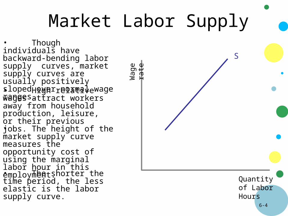
• Though individuals have backward-bending labor supply curves, market supply curves are usually positively sloped over normal wage ranges.

• High relative wages attract workers away from household production, leisure, or their previous jobs.

• The height of the market supply curve measures the opportunity cost of using the marginal labor hour in this employment.

S

• The shorter the time period, the less elastic is the labor supply curve.

6-5

Wage and Employment Determination


Wage rate

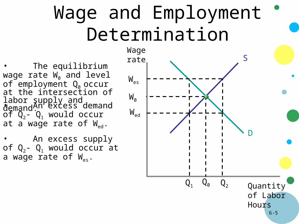
• The equilibrium wage rate W0 and level of employment Q0 occur at the intersection of labor supply and demand.

• An excess demand of Q2- Q1 would occur at a wage rate of Wed.

• An excess supply of Q2- Q1 would occur at a wage rate of Wes.

S

D

Q0

W0

Wed

Q2Q1

Wes

6-6

Labor Supply Determinants

o Other wage rates• If wages in other occupations rise (fall), then

labor supply will fall (rise).

o Nonwage income• If nonwage income rises (falls), then labor

supply will fall (rise).

o Preferences for work versus leisure• If preferences for work increase (decrease),

then labor supply will increase (decrease).

6-7

Labor Supply Determinants

o Nonwage aspects of job• If the nonwage aspects of a job improve

(worsen), then labor supply will increase (decrease).

o Number of qualified suppliers• An increase (decrease) in the number of

qualified workers will increase (decrease) labor supply.

6-8

Labor Demand Determinantso Product demand

• Changes in product demand that increase (decrease) the product price, will increase (decrease) labor demand.

o Productivity• An increase (decrease) in productivity will

increase (decrease) labor demand, assuming that it does not cause an offset in the product price.

6-9

Labor Demand Determinants

o Prices of other resources• For gross substitutes, an increase

(decrease) in the price of a substitute input will increase (decrease) labor demand.

• For gross complements, an increase (decrease) in the price of a complement input will decrease (increase) labor demand.

6-10

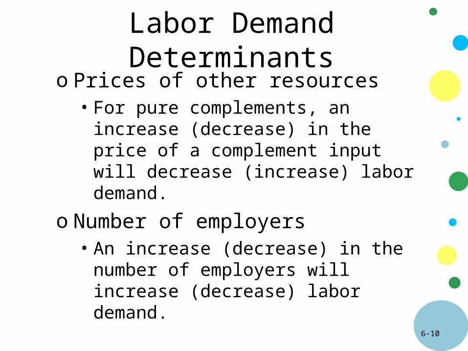
Labor Demand Determinantso Prices of other resources

• For pure complements, an increase (decrease) in the price of a complement input will decrease (increase) labor demand.

o Number of employers • An increase (decrease) in the number of

employers will increase (decrease) labor demand.

6-11

Changes in Labor Demand


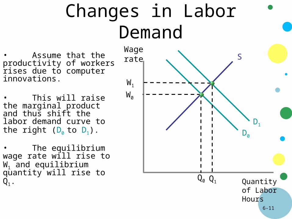
Wage rate• Assume that the productivity of workers rises due to computer innovations.

• This will raise the marginal product and thus shift the labor demand curve to the right (D0 to D1).

• The equilibrium wage rate will rise to W1 and equilibrium quantity will rise to Q1.

S

D0

Q0

W0

D1

Q1

W1

6-12

Changes in Labor Supply


Wage rate

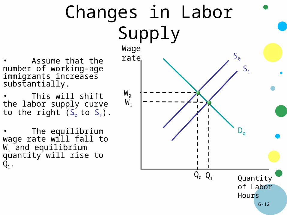
• Assume that the number of working-age immigrants increases substantially.

• This will shift the labor supply curve to the right (S0 to S1).

• The equilibrium wage rate will fall to W1 and equilibrium quantity will rise to Q1.

S0

D0

Q0

W0

S1

Q1

W1

6-13

Wage and Employment for a Perfectly Competitive Firm


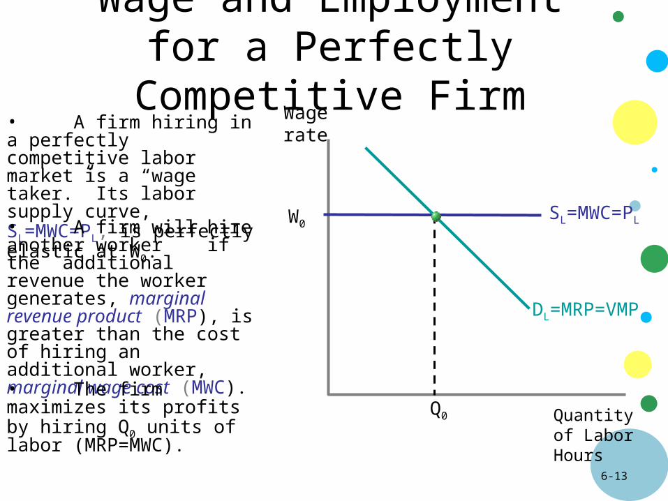
Wage rate• A firm hiring in a perfectly competitive labor market is a “wage taker.” Its labor supply curve, SL=MWC=PL, is perfectly elastic at W0.

• A firm will hire another worker if the additional revenue the worker generates, marginal revenue product (MRP), is greater than the cost of hiring an additional worker, marginal wage cost (MWC).

SL=MWC=PL

DL=MRP=VMP

Q0

W0

• The firm maximizes its profits by hiring Q0 units of labor (MRP=MWC).

6-14

Allocative Efficiencyo An efficient allocation of labor is

obtained when society gets the largest possible amount of output from a given amount of labor.

o Efficient allocation requires the VMP of labor for each product be equal to the price of labor.

o Perfect competition in the product and labor markets creates allocative efficiency.

6-15

Questions for Thought1. What effect will each of the following have on

the market demand for a specific type of labor:

(a) An increase in product demand that increases the product price.

(b) A decline in the productivity of this type of labor.

(c) An increase in the price of a gross substitute of labor.

(e) The demise of several firms that hire this type of labor.

(f) A decline in the market wage for this type of labor.

(d) An increase in the price of a gross complement of labor.

6-16

2. Wage and Employment Determination: Monopoly in the Product Market

6-17

Wage and Employment for a Monopolist


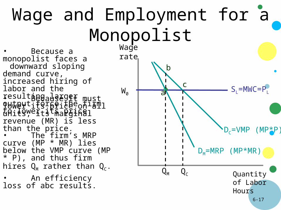
Wage rate• Because a monopolist faces a downward sloping demand curve, increased hiring of labor and the resulting larger output force the firm to lower its price.

• Because it must lower its price on all units, its marginal revenue (MR) is less than the price.

SL=MWC=PL

DC=VMP (MP*P)

QC

W0

• The firm’s MRP curve (MP * MR) lies below the VMP curve (MP * P), and thus firm hires QM rather than QC.

DM=MRP (MP*MR)

a

b

c

QM• An efficiency loss of abc results.

6-18

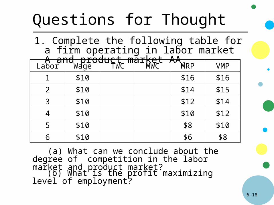
1. Complete the following table for a firm operating in labor market A and product market AA.

Questions for Thought

Labor Wage TWC MWC MRP VMP

1 $10 $16 $16

2 $10 $14 $15

3 $10 $12 $14

4 $10 $10 $12

5 $10 $8 $10

6 $10 $6 $8

(a) What can we conclude about the degree of competition in the labor market and product market?

(b) What is the profit maximizing level of employment?

6-19

3. Monopsony

6-20

Monopsony

o A monopsony is a labor market where a single firm is the sole hirer of a particular type of labor.• A monopsonist has control over

the wage rate workers are paid by hiring more or less labor.

6-21

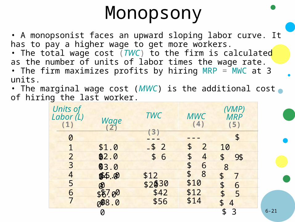
$ 2 $ 6

$12 $20 $30 $42 $56

-----

TWC (3)

$ 7

$ 9 $ 8

$ 3

(VMP)MRP(5)

$ 6 $ 5 $ 4

$ 10

• A monopsonist faces an upward sloping labor curve. It has to pay a higher wage to get more workers. • The total wage cost (TWC) to the firm is calculated as the number of units of labor times the wage rate. • The firm maximizes profits by hiring MRP = MWC at 3 units.• The marginal wage cost (MWC) is the additional cost of hiring the last worker.

Monopsony

MWC (4)

---$ 2$ 4$ 6$ 8$10$12$14

Wage(2)

Units of Labor

(L)(1) 0 1 2 3 4 5 6 7

$1.00 $2.00 $3.00 $4.00$5.00

$6.00$7.00$8.00

6-22

Wage and Employment for a Monopsonist


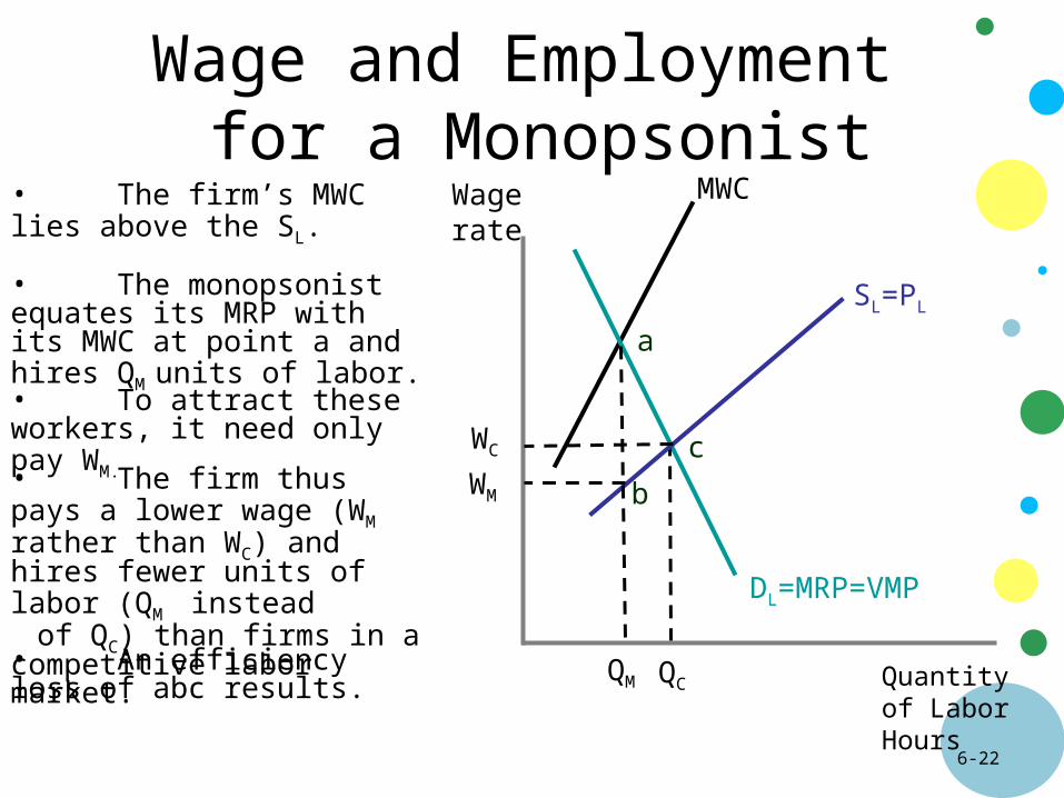
Wage rate• The firm’s MWC lies above the SL.

• To attract these workers, it need only pay WM.

SL=PL

QC

• The firm thus pays a lower wage (WM rather than WC) and hires fewer units of labor (QM instead of QC) than firms in a competitive labor market. DL=MRP=VMP

• An efficiency loss of abc results.

MWC

WC

QM

WM

• The monopsonist equates its MRP with its MWC at point a and hires QM units of labor.

b

a

c

6-23

4. Wage Determination: Delayed Supply Responses

6-24

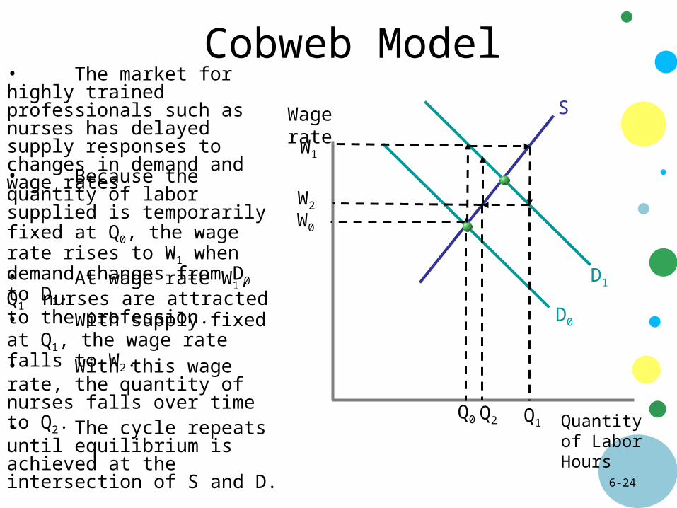
Cobweb Model• The market for highly trained professionals such as nurses has delayed supply responses to changes in demand and wage rates.

Q0

W0

D0


Wage rate S

• Because the quantity of labor supplied is temporarily fixed at Q0, the wage rate rises to W1 when demand changes from D0 to D1.• At wage rate W1, Q1 nurses are attracted to the profession. • With supply fixed at Q1, the wage rate falls to W2.• With this wage rate, the quantity of nurses falls over time to Q2.• The cycle repeats until equilibrium is achieved at the intersection of S and D.

D1

W1

W2

Q1Q2

6-25

Evidence

o Some evidence exists for cobweb adjustments in markets such as lawyers and engineers.

o Critics argue that:• Students make choices on the basis of the

lifetime earnings stream rather than starting salaries.

• Students make a forecast of the long-run outcome of a change in demand or supply and make the right choice.

Education

Wage Determination and the Allocation of Labor