Statistics assignment help service

Statistics Assignment Help Service Statistics Homework Help Service

Statistics Help Desk Mark Austin

Contact Us:

Web: http://economicshelpdesk.com/

Email: [email protected]

Twitter: https://twitter.com/econ_helpdesk Facebook: https://www.facebook.com/economicshelpdesk

Tel: +44-793-744-3379

Copyright © 2012-2014 Economicshelpdesk.com, All rights reserved

http://economicshelpdesk.com/

mailto:[email protected]

https://twitter.com/econ_helpdesk

https://www.facebook.com/economicshelpdesk


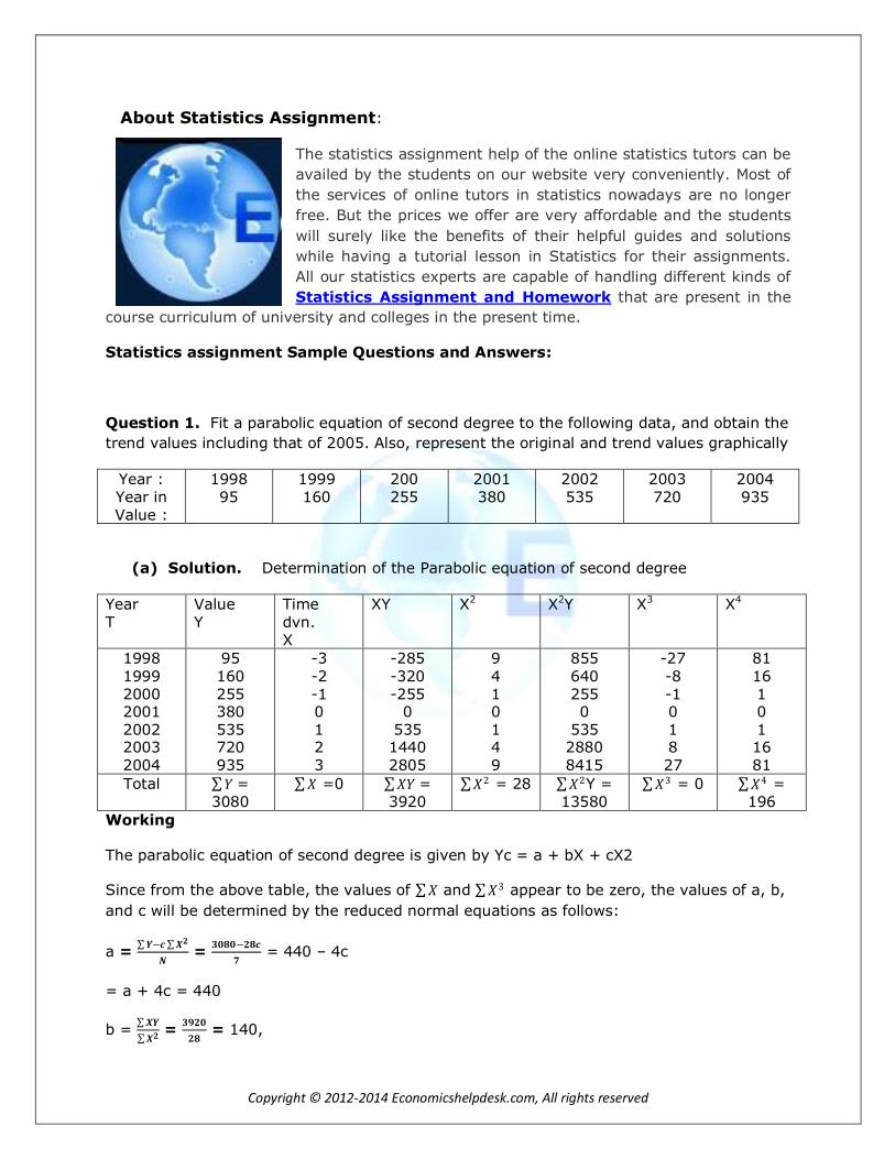
About Statistics Assignment:

The statistics assignment help of the online statistics tutors can be

availed by the students on our website very conveniently. Most of

the services of online tutors in statistics nowadays are no longer

free. But the prices we offer are very affordable and the students

will surely like the benefits of their helpful guides and solutions

while having a tutorial lesson in Statistics for their assignments.

All our statistics experts are capable of handling different kinds of

Statistics Assignment and Homework that are present in the

course curriculum of university and colleges in the present time.

Statistics assignment Sample Questions and Answers:

Question 1. Fit a parabolic equation of second degree to the following data, and obtain the

trend values including that of 2005. Also, represent the original and trend values graphically

Year : Year in Value :

1998 95

1999 160

200 255

2001 380

2002 535

2003 720

2004 935

(a) Solution. Determination of the Parabolic equation of second degree

Year T

Value Y

Time dvn. X

XY X2 X2Y X3 X4

1998

1999 2000 2001 2002 2003 2004

95

160 255 380 535 720 935

-3

-2 -1 0 1 2 3

-285

-320 -255

0 535 1440 2805

9

4 1 0 1 4 9

855

640 255 0

535 2880 8415

-27

-8 -1 0 1 8 27

81

16 1 0 1 16 81

Total 𝑌 =

3080

𝑋 =0 𝑋𝑌 =

3920

𝑋2 = 28 𝑋2Y =

13580

𝑋3 = 0 𝑋4 =

196

Working

The parabolic equation of second degree is given by Yc = a + bX + cX2

Since from the above table, the values of 𝑋 and 𝑋3 appear to be zero, the values of a, b,

and c will be determined by the reduced normal equations as follows:

a = 𝒀−𝒄 𝑿𝟐

𝑵 =

𝟑𝟎𝟖𝟎−𝟐𝟖𝒄

𝟕 = 440 – 4c

= a + 4c = 440

b = 𝑿𝒀

𝑿𝟐 =

𝟑𝟗𝟐𝟎

𝟐𝟖 = 140,

http://economicshelpdesk.com/statistics-assignment-homework-help.php


and

c = 𝑿𝟐𝒀−𝒂 𝑿𝟐

𝑿𝟒 =

𝟏𝟑𝟓𝟖𝟎−𝟐𝟖𝒂

𝟏𝟗𝟔 =

𝟒𝟖𝟓−𝒂

𝟕

= a + 7c = 485

Subtracting the eqn (i) from the eqn (iii) we get,

a + 7c = 485 (-) a + 4c = 440 3c = 45

∴ c = 15

Putting the value of c in the equation (i) we get,

a + 4(15) = 440

= a = 440 – 60 = 380

Thus, a = 380, b – 140, and c = 15

Putting the above values of the constants a, b, and c in the equation, we get the parabolic

equation of the second degree fitted as under:

Yc = 380 + 140X + 15X2

Where, X unit = time deviation, Y unit = annual value, and the trend origin is 2001.

Using the above parabola we obtain the trend values as under:


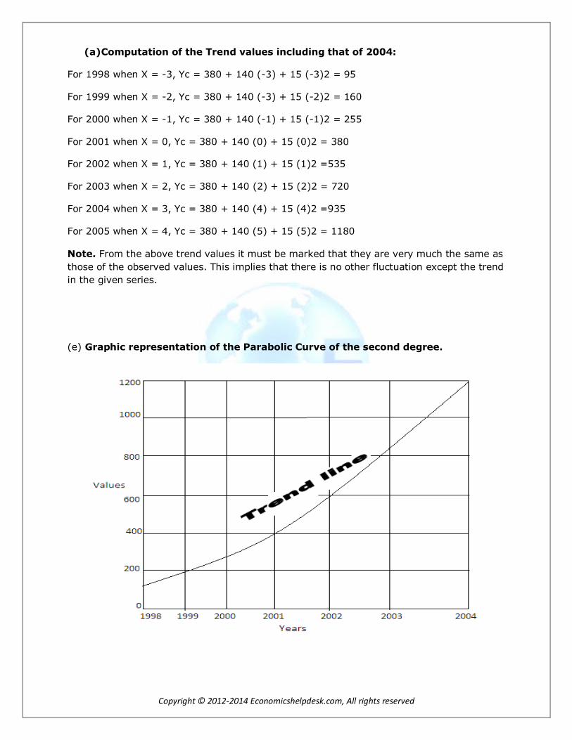
(a) Computation of the Trend values including that of 2004:

For 1998 when X = -3, Yc = 380 + 140 (-3) + 15 (-3)2 = 95

For 1999 when X = -2, Yc = 380 + 140 (-3) + 15 (-2)2 = 160

For 2000 when X = -1, Yc = 380 + 140 (-1) + 15 (-1)2 = 255

For 2001 when X = 0, Yc = 380 + 140 (0) + 15 (0)2 = 380

For 2002 when X = 1, Yc = 380 + 140 (1) + 15 (1)2 =535

For 2003 when X = 2, Yc = 380 + 140 (2) + 15 (2)2 = 720

For 2004 when X = 3, Yc = 380 + 140 (4) + 15 (4)2 =935

For 2005 when X = 4, Yc = 380 + 140 (5) + 15 (5)2 = 1180

Note. From the above trend values it must be marked that they are very much the same as

those of the observed values. This implies that there is no other fluctuation except the trend

in the given series.

(e) Graphic representation of the Parabolic Curve of the second degree.


Vii. Geometric, or Logarithmic Method of the Least square

Under this method, the trend equation is obtained Yc = aXb

Using the logarithms, the above equation is modified as under :

Log Yc = Log a + b log X

The above geometric curve equation should not, however, be used unless there is a clear

geometric progression in the value variable of a time series. Further, while using the

logarithm of X, the X origin cannot be taken at the middle of the period. This limitation is

overcome by the exponential trend fitting discussed below. The above trend equation can

also be put in the following modified form :

Yc = aXb + k

Using the logarithms, the modified form of the above can be presented as under :

Yc = {Anti log of (log a + b log X)} + k

Where, k is a constant

However, this method is rarely used in practice.

Vii. Exponential Method of the Least Square.

This method of trend fitting is resorted to only when the value variable Y shows a geometric

progression viz : 1,2,4,8,16,32, and so on, and the time variable (t) shows an arithmetic

progression viz : 1,2,3,4,5,6 and the like In such cases, the trend line is to be drawn on a

semi-logarithmic chart in the form of a straight line, or a non-linear curve to show the

increase, or decrease of the value of variable Y at a constant rate rather than a constant

amount. When the trend takes the form of a non-linear curve on a semi-logarithmic chart,

an upward curve indicates the increase at varying rates depending upon the shapes of the

slopes. The steeper the slope, the higher is the rate of increase.

However, under this method, the trend line is fitted by the following model:

Yc = abX

Using logarithmic operation, the above equation is modified as under :

Yc = A.L. (log a + X log b)

In the above equation, a and b are the two constants the values of which are determined by

solving the following two normal equations and finding the antilogarithms thereof:

log 𝑦 = N log a + log b 𝑋

𝑋 log 𝑦 = log a 𝑋 + log b 𝑋2

If by taking the time deviations X from the mid-point of the time variable t, 𝑋 could be

made zero, the logarithm of the two constants a and b can be determined directly as under:

Log a = log 𝑌

𝑋2


Log b = Xlog 𝑌

𝑋2

After obtaining the values of a and b in the above manner, and substituting their values in

the equation Yc = abX, we can fit the trend line equation under this method, and with such

an equation we can very well estimate the trend values of the time series, and predict the

value for any past and future year as well.

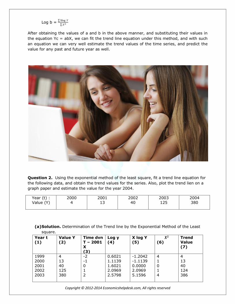
Question 2. Using the exponential method of the least square, fit a trend line equation for

the following data, and obtain the trend values for the series. Also, plot the trend lien on a

graph paper and estimate the value for the year 2004.

Year (t) : Value (Y)

2000 4

2001 13

2002 40

2003 125

2004 380

(a) Solution. Determination of the Trend line by the Exponential Method of the Least

square.

Year t (1)

Value Y (2)

Time dvn T – 2001 X (3)

Log y (4)

X log Y (5)

𝑿𝟐 (6)

Trend Value (7)

1999 2000 2001 2002

2003

4 13 40 125

380

-2 -1 0 1

2

0.6021 1.1139 1.6021 2.0969

2.5798

-1.2042 -1.1139 0.0000 2.0969

5.1596

4 1 0 1

4

4 13 40 124

386


Working

The exponential trend line is given by

Yc = abX

= AL (log a + X log b)

Since 𝑋 = 0, the logarithm of a and b the two constants in the above equation are directly

computed as under:

Log a = 𝑙𝑜𝑔𝑌

𝑁 =

7.9948

5 = 1.5990 app.

And log b = 𝑋𝑙𝑜𝑔𝑌

𝑋2 = 4.9384

10 = 0.4938 app.

Putting the above logs of a and b in the equation, we get the exponential trend lien titled as

under. :

Yc = AL ( 1.5990 + 0.4938X)

Where, X = time deviation, Y = annual value and 2002 is the trend origin i.e. the origin of

X. With the above equation, the trend values are computed as under:

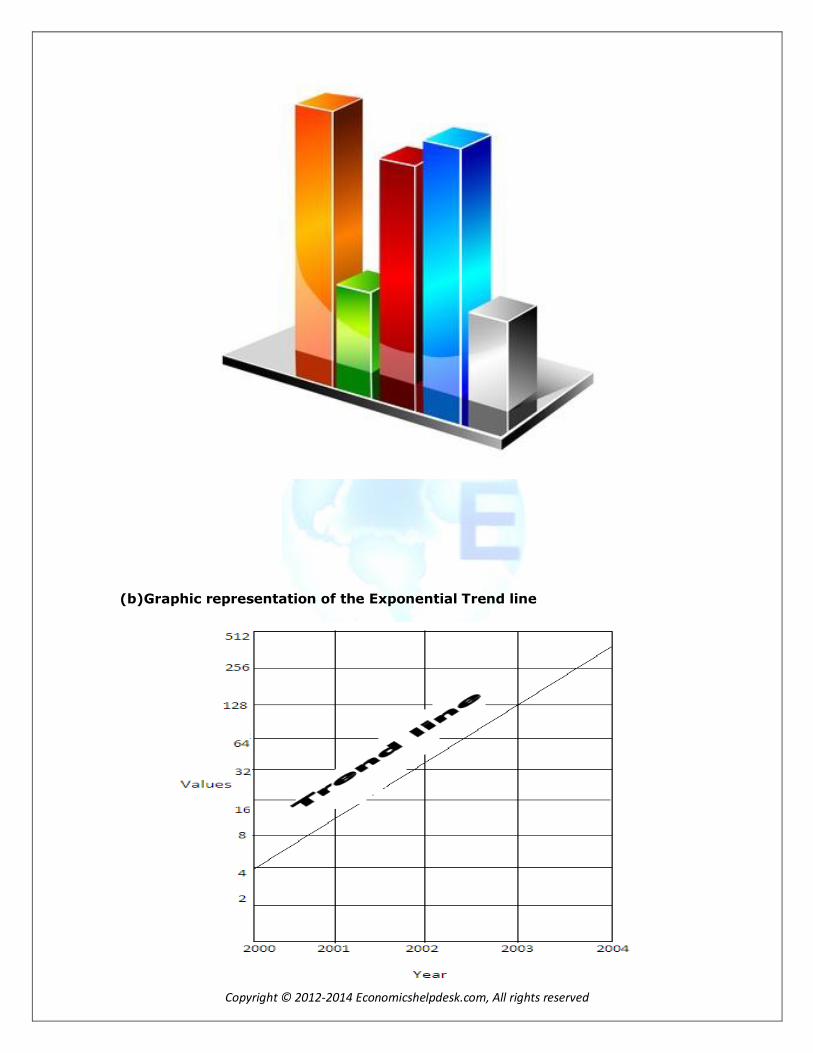
(b)Computation of the Trend Values (as shown in the column 7 of the Table)

For 2000 when X = -2, Yc = AL [1.5990 + 0.4938 (-2)] = 4.087 = 4

For2001 when X = -1, Yc = AL [1.5990 + 0.4938 (-1)] = 12.750 = 13

For 2002 when X = 0, AL [1.5990 + 0.4938 (0)] = 39.72 = 40

For 2003 when X = 1, AL [1.5990 + 0.4938 (1)] = 123.8 = 124

For 2004 when X = 2, Yc = AL [1.5990 + 0.4938 (2)] 386.0 = 386

From the above results, it must be seen that the trend values almost approach the observed

values. The slight difference that appear between some of them are due to the error of

approximation involved in the logarithms.


(b) Graphic representation of the Exponential Trend line


(c) Forecasting the value for 2005

For 2005, X = 3

Thus, when X = 3, Yc = AL [1.5990 + 0.4938(3)] = 1203

Ix. Growth Curve Method of the Least Square.

The growth curves are some special type of curves which are plotted on graph papers for

analysis and estimation the trend values in the business and economic phenomena. Where

initially, the growth rate is very slow but gradually it picks up at a faster rate till it reaches a

point of stagnation, or saturation. Such situations are quite common in business fields

where new products are introduced for marketing. In such a situation, when a new product

say the book, “Statistical Methods” is introduced into the market, the growth rate of its sale

quite slow, and if the product proves to be worthwhile, the growth rate of its sale gradually

goes up fast and reaches relatively a higher level, and then it begins to decline. As such, a

curve representing this type of phenomena continues to grow more and more slowly

approaching the upper limit, but never reaching the same. It takes the shape of an

elongated f which indicates the pattern of growth in terms of the actual amount as small in

the early years increasingly greater in the middle years, and large but stabilized in the later

years. But when such curves are plotted on a semi logarithmic chart, they show a growth at

rapidly increasing rates in the earlier periods, and at a declining ratio in the later periods of

the series.

There are different types of growth curves used in different fields of business. And

economics, but the most popular among them are the following twos which have come into

being since 1920 :

1. Geometric Growth Curve.

2. Logistic or Pearl-Read Growth Curve.

A brief introduction to these curve is given as belows:

1. Gompertz Growth Curve. The fundamental trend equation of this curve is given by Yc

= kabx

When put to the logarithmic form, the above equation is modified as under:

Ye = AL of [log K + bX lag a]

Where, k represents the constant of the highest point, a the intercept of y i.e. the trend

value of the origin of X, and b the slope of the line i.e. the rate of growth.

2. Logistic, or Pearl-Read Growth Curve.

This curve is given by the following model

𝟏

𝒀𝒄 = K + abX

The above equation may also be used in the alternative form as under :

Yc = 𝑲

𝟏+ 𝟏𝟎𝒂+𝒃𝑿 ,or 𝑲

𝟏+ 𝒆𝒂+𝒃𝑿


It may be noted that the Logistic curve is nothing but a modified exponential curve in terms

of the reciprocal of the Y variable. This curve, however, is very popular in the demographic

studies and in many business and economic analysis.

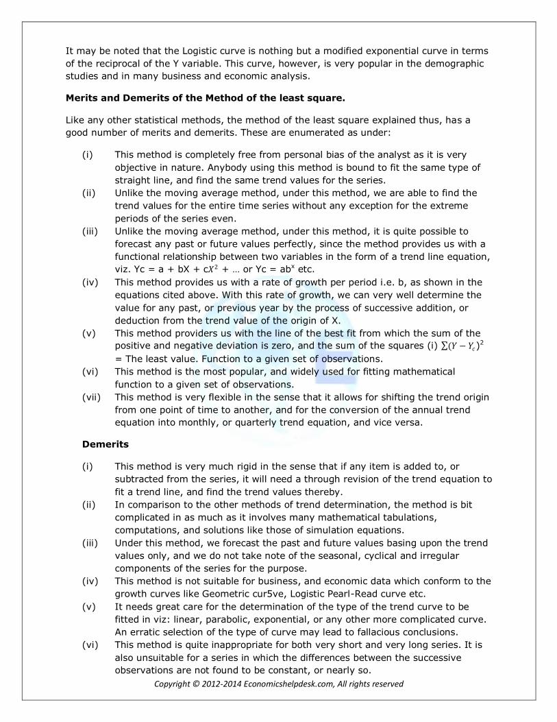
Merits and Demerits of the Method of the least square.

Like any other statistical methods, the method of the least square explained thus, has a

good number of merits and demerits. These are enumerated as under:

(i) This method is completely free from personal bias of the analyst as it is very

objective in nature. Anybody using this method is bound to fit the same type of

straight line, and find the same trend values for the series.

(ii) Unlike the moving average method, under this method, we are able to find the

trend values for the entire time series without any exception for the extreme

periods of the series even.

(iii) Unlike the moving average method, under this method, it is quite possible to

forecast any past or future values perfectly, since the method provides us with a

functional relationship between two variables in the form of a trend line equation,

viz. Yc = a + bX + c𝑋2 + … or Yc = abx etc.

(iv) This method provides us with a rate of growth per period i.e. b, as shown in the

equations cited above. With this rate of growth, we can very well determine the

value for any past, or previous year by the process of successive addition, or

deduction from the trend value of the origin of X.

(v) This method providers us with the line of the best fit from which the sum of the

positive and negative deviation is zero, and the sum of the squares (i) (𝑌 − 𝑌𝑐)2

= The least value. Function to a given set of observations.

(vi) This method is the most popular, and widely used for fitting mathematical

function to a given set of observations.

(vii) This method is very flexible in the sense that it allows for shifting the trend origin

from one point of time to another, and for the conversion of the annual trend

equation into monthly, or quarterly trend equation, and vice versa.

Demerits

(i) This method is very much rigid in the sense that if any item is added to, or

subtracted from the series, it will need a through revision of the trend equation to

fit a trend line, and find the trend values thereby.

(ii) In comparison to the other methods of trend determination, the method is bit

complicated in as much as it involves many mathematical tabulations,

computations, and solutions like those of simulation equations.

(iii) Under this method, we forecast the past and future values basing upon the trend

values only, and we do not take note of the seasonal, cyclical and irregular

components of the series for the purpose.

(iv) This method is not suitable for business, and economic data which conform to the

growth curves like Geometric cur5ve, Logistic Pearl-Read curve etc.

(v) It needs great care for the determination of the type of the trend curve to be

fitted in viz: linear, parabolic, exponential, or any other more complicated curve.

An erratic selection of the type of curve may lead to fallacious conclusions.

(vi) This method is quite inappropriate for both very short and very long series. It is

also unsuitable for a series in which the differences between the successive

observations are not found to be constant, or nearly so.


Shifting of a Trend Origin and Conversion of the Trend Equation

Shifting of a Trend Origin.

By shifting of a trend origin we mean changing the origin of X (the time from which time

deviations are taken) from one point of time to another point of time, whether earlier or

later to the present origin. This becomes necessary at times to facilitate comparison in

the trend values. To give effect to such shifting, the trend equation that is already fitted

is slightly modified by adding to, or subtracting from X, the time difference between the

existing origin and the proposed origin. In case, the shifting is made to a later period,

the difference in time is added to X, and in case, it is made to an earlier period, the

difference in time is subtracted from X. Thus the fitted trend equation is modified as

under:

Yc = a + b (X ± K).

Where, K represents the time difference in shifting.

By such modifications in a linear equation, the value of a (i.e. the value of the trend

origin) only, is affected and the value of b (i.e. the slope of the change) remains as it is.

But in a parabolic equation of second degree, such modification will affect the value of

both a and b, but not the value of c (i.e. the rate of change in slope).


Question 3. Shift the trend origin form 2001 to 2004 in the straight line trend equation,

Yc = 25 + 2X, given that the time unit = 1 Year.

Solution:

Here, the trend origin is to be shifted forward by 3 years i.e. from 2001 to 2004. Thus K =3

By the formula of trend shifting we have,

Yc = a + b (X + K)

Substituting the respective values in the above we get, Yc = 25 + 2 (X +3)

= 25 + 2X + 6

= 31 + 2X

Thus, the shifted equation is given by

Yc = 31 + 2X

Where, origin of X = 2004, and

X unit = 1 Year.

Note. From the above shifted equation, it must be noted that the value of a only has

been changed from 25 to 31, whereas the value of b remains the same 2.

Education

Statistics assignment help service