1

Programming in Matlab – lesson 5 -----------------------------------------------------------------

5.1 Image Processing Toolbox

5.1 Image Processing Toolbox

Introduction The Image Processing Toolbox software is a collection of functions that extend the capability of the MATLAB numeric computing environment. The toolbox supports a wide range of image processing operations, including

• • Spatial image transformations • • Morphological operations • • Neighborhood and block operations • • Linear filtering and filter design • • Transforms • • Image analysis and enhancement • • Image registration • • Deblurring • • Region of interest operations

Images in MATLAB The basic data structure in MATLAB is the array, an ordered set of real or complex elements. This object is naturally suited to the representation of images, real-valued ordered sets of color or intensity data. MATLAB stores most images as two-dimensional arrays (i.e., matrices), in which each element of the matrix corresponds to a single pixel in the displayed image. (Pixel is derived from picture element and usually denotes a single dot on a computer display.) For example, an image composed of 200 rows and 300 columns of different colored dots would be stored in MATLAB as a 200-by-300 matrix. Some images, such as truecolor images, require a three-dimensional array, where the first plane in the third dimension represents the red pixel intensities, the second plane represents the green pixel intensities, and the third plane represents the blue pixel intensities. This convention makes working with images in MATLAB similar to working with any other type of matrix data, and makes the full power of MATLAB available for image processing applications.

Image Coordinate Systems

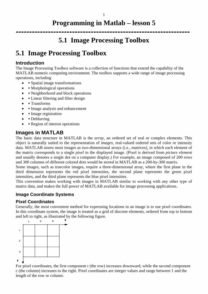
Pixel Coordinates Generally, the most convenient method for expressing locations in an image is to use pixel coordinates. In this coordinate system, the image is treated as a grid of discrete elements, ordered from top to bottom and left to right, as illustrated by the following figure.

For pixel coordinates, the first component r (the row) increases downward, while the second component c (the column) increases to the right. Pixel coordinates are integer values and range between 1 and the length of the row or column.

2

Image Types in the Toolbox

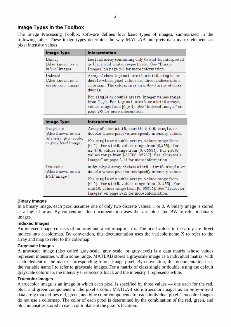
The Image Processing Toolbox software defines four basic types of images, summarized in the following table. These image types determine the way MATLAB interprets data matrix elements as pixel intensity values

Binary Images In a binary image, each pixel assumes one of only two discrete values: 1 or 0. A binary image is stored as a logical array. By convention, this documentation uses the variable name BW to refer to binary images.

Indexed Images An indexed image consists of an array and a colormap matrix. The pixel values in the array are direct indices into a colormap. By convention, this documentation uses the variable name X to refer to the array and map to refer to the colormap.

Grayscale Images A grayscale image (also called gray-scale, gray scale, or gray-level) is a data matrix whose values represent intensities within some range. MATLAB stores a grayscale image as a individual matrix, with each element of the matrix corresponding to one image pixel. By convention, this documentation uses the variable name I to refer to grayscale images. For a matrix of class single or double, using the default grayscale colormap, the intensity 0 represents black and the intensity 1 represents white.

Truecolor Images A truecolor image is an image in which each pixel is specified by three values — one each for the red, blue, and green components of the pixel’s color. MATLAB store truecolor images as an m-by-n-by-3 data array that defines red, green, and blue color components for each individual pixel. Truecolor images do not use a colormap. The color of each pixel is determined by the combination of the red, green, and blue intensities stored in each color plane at the pixel’s location.

3 Example 1 — Some Basic Concepts This example introduces some basic image processing concepts. The example starts by reading an image into the MATLAB workspace. The example then performs some contrast adjustment on the image. Finally, the example writes the adjusted image to a file.

Step 1: Read and Display an Image First, clear the MATLAB workspace of any variables and close open figure windows.

>>close all To read an image, use the imread command. The example reads one of the sample images included with the toolbox, pout.tif, and stores it in an array named I.

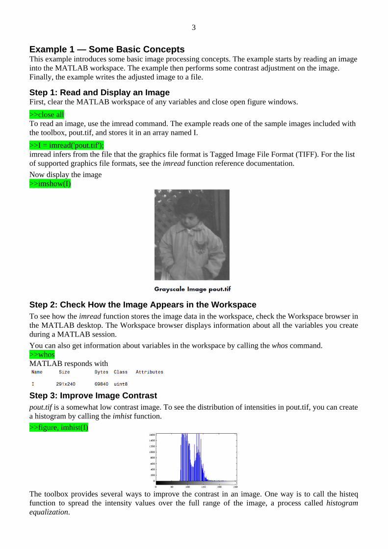
>>I = imread('pout.tif'); imread infers from the file that the graphics file format is Tagged Image File Format (TIFF). For the list of supported graphics file formats, see the imread function reference documentation.

Now display the image >>imshow(I)

Step 2: Check How the Image Appears in the Workspace

To see how the imread function stores the image data in the workspace, check the Workspace browser in the MATLAB desktop. The Workspace browser displays information about all the variables you create during a MATLAB session.

You can also get information about variables in the workspace by calling the whos command. >>whos MATLAB responds with

Step 3: Improve Image Contrast

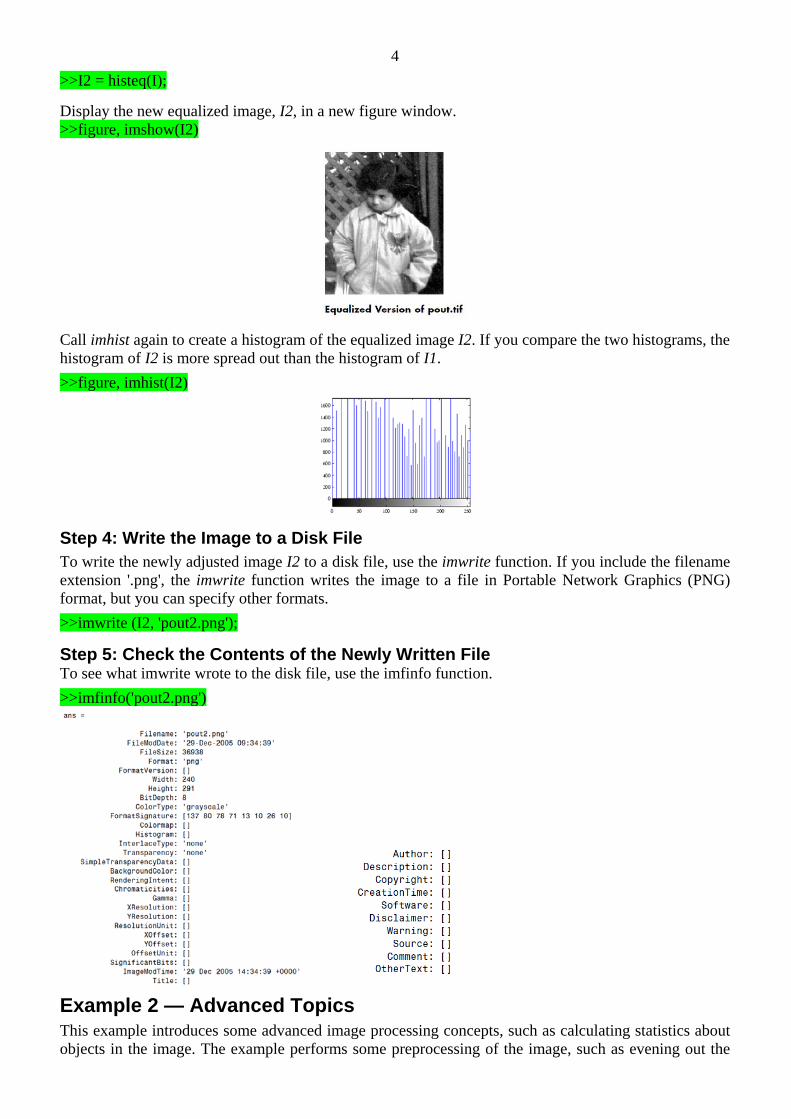
pout.tif is a somewhat low contrast image. To see the distribution of intensities in pout.tif, you can create a histogram by calling the imhist function.

>>figure, imhist(I)

The toolbox provides several ways to improve the contrast in an image. One way is to call the histeq function to spread the intensity values over the full range of the image, a process called histogram equalization.

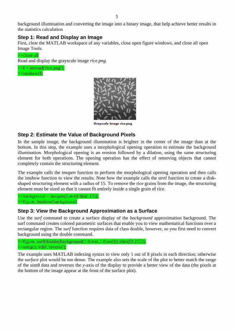
4>>I2 = histeq(I); Display the new equalized image, I2, in a new figure window. >>figure, imshow(I2)

Call imhist again to create a histogram of the equalized image I2. If you compare the two histograms, the histogram of I2 is more spread out than the histogram of I1.

>>figure, imhist(I2)

Step 4: Write the Image to a Disk File

To write the newly adjusted image I2 to a disk file, use the imwrite function. If you include the filename extension '.png', the imwrite function writes the image to a file in Portable Network Graphics (PNG) format, but you can specify other formats.

>>imwrite (I2, 'pout2.png');

Step 5: Check the Contents of the Newly Written File To see what imwrite wrote to the disk file, use the imfinfo function.

>>imfinfo('pout2.png')

Example 2 — Advanced Topics

This example introduces some advanced image processing concepts, such as calculating statistics about objects in the image. The example performs some preprocessing of the image, such as evening out the

5background illumination and converting the image into a binary image, that help achieve better results in the statistics calculation

Step 1: Read and Display an Image First, clear the MATLAB workspace of any variables, close open figure windows, and close all open Image Tools.

>>close all Read and display the grayscale image rice.png.

>>I = imread('rice.png'); >>imshow(I)

Step 2: Estimate the Value of Background Pixels

In the sample image, the background illumination is brighter in the center of the image than at the bottom. In this step, the example uses a morphological opening operation to estimate the background illumination. Morphological opening is an erosion followed by a dilation, using the same structuring element for both operations. The opening operation has the effect of removing objects that cannot completely contain the structuring element. The example calls the imopen function to perform the morphological opening operation and then calls the imshow function to view the results. Note how the example calls the strel function to create a disk-shaped structuring element with a radius of 15. To remove the rice grains from the image, the structuring element must be sized so that it cannot fit entirely inside a single grain of rice.

>>background = imopen(I,strel('disk',15)); >>figure, imshow(background)

Step 3: View the Background Approximation as a Surface

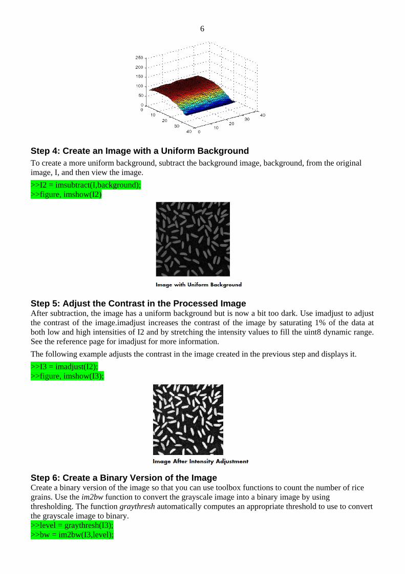
Use the surf command to create a surface display of the background approximation background. The surf command creates colored parametric surfaces that enable you to view mathematical functions over a rectangular region. The surf function requires data of class double, however, so you first need to convert background using the double command.

>>figure, surf(double(background(1:8:end,1:8:end))),zlim([0 255]); >>set(gca,'ydir','reverse');

The example uses MATLAB indexing syntax to view only 1 out of 8 pixels in each direction; otherwise the surface plot would be too dense. The example also sets the scale of the plot to better match the range of the uint8 data and reverses the y-axis of the display to provide a better view of the data (the pixels at the bottom of the image appear at the front of the surface plot).

6

Step 4: Create an Image with a Uniform Background

To create a more uniform background, subtract the background image, background, from the original image, I, and then view the image.

>>I2 = imsubtract(I,background); >>figure, imshow(I2)

Step 5: Adjust the Contrast in the Processed Image After subtraction, the image has a uniform background but is now a bit too dark. Use imadjust to adjust the contrast of the image.imadjust increases the contrast of the image by saturating 1% of the data at both low and high intensities of I2 and by stretching the intensity values to fill the uint8 dynamic range. See the reference page for imadjust for more information.

The following example adjusts the contrast in the image created in the previous step and displays it.

>>I3 = imadjust(I2); >>figure, imshow(I3);

Step 6: Create a Binary Version of the Image Create a binary version of the image so that you can use toolbox functions to count the number of rice grains. Use the im2bw function to convert the grayscale image into a binary image by using thresholding. The function graythresh automatically computes an appropriate threshold to use to convert the grayscale image to binary. >>level = graythresh(I3); >>bw = im2bw(I3,level);

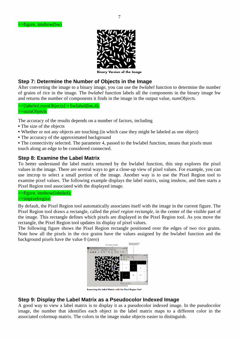
7>>figure, imshow(bw)

Step 7: Determine the Number of Objects in the Image After converting the image to a binary image, you can use the bwlabel function to determine the number of grains of rice in the image. The bwlabel function labels all the components in the binary image bw and returns the number of components it finds in the image in the output value, numObjects.

>>[labeled,numObjects] = bwlabel(bw,4); >>numObjects The accuracy of the results depends on a number of factors, including • The size of the objects • Whether or not any objects are touching (in which case they might be labeled as one object) • The accuracy of the approximated background • The connectivity selected. The parameter 4, passed to the bwlabel function, means that pixels must touch along an edge to be considered connected.

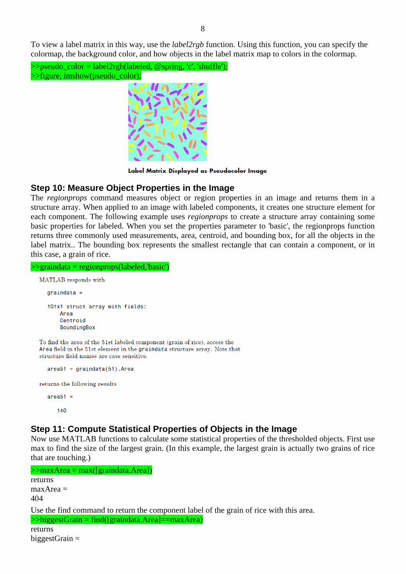
Step 8: Examine the Label Matrix To better understand the label matrix returned by the bwlabel function, this step explores the pixel values in the image. There are several ways to get a close-up view of pixel values. For example, you can use imcrop to select a small portion of the image. Another way is to use the Pixel Region tool to examine pixel values. The following example displays the label matrix, using imshow, and then starts a Pixel Region tool associated with the displayed image.

>>figure, imshow(labeled); >>impixelregion

By default, the Pixel Region tool automatically associates itself with the image in the current figure. The Pixel Region tool draws a rectangle, called the pixel region rectangle, in the center of the visible part of the image. This rectangle defines which pixels are displayed in the Pixel Region tool. As you move the rectangle, the Pixel Region tool updates its display of pixel values. The following figure shows the Pixel Region rectangle positioned over the edges of two rice grains. Note how all the pixels in the rice grains have the values assigned by the bwlabel function and the background pixels have the value 0 (zero)

Step 9: Display the Label Matrix as a Pseudocolor Indexed Image A good way to view a label matrix is to display it as a pseudocolor indexed image. In the pseudocolor image, the number that identifies each object in the label matrix maps to a different color in the associated colormap matrix. The colors in the image make objects easier to distinguish.

8

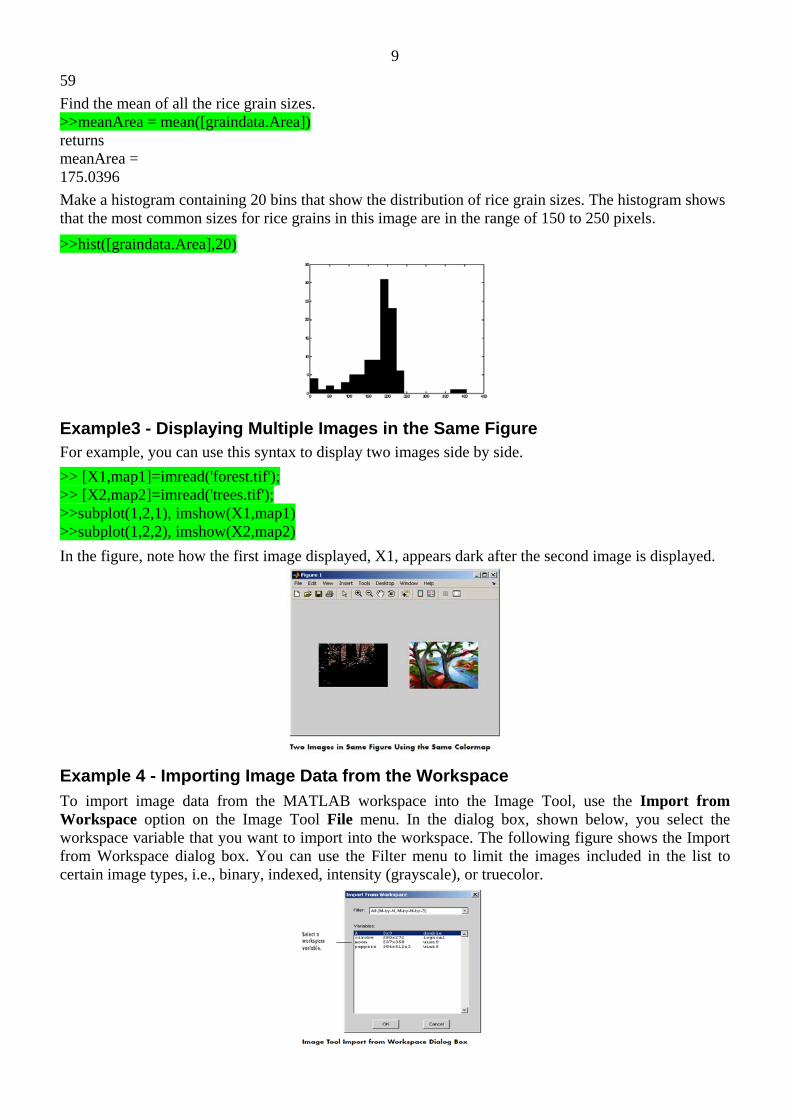
To view a label matrix in this way, use the label2rgb function. Using this function, you can specify the colormap, the background color, and how objects in the label matrix map to colors in the colormap.

>>pseudo_color = label2rgb(labeled, @spring, 'c', 'shuffle'); >>figure, imshow(pseudo_color);

Step 10: Measure Object Properties in the Image The regionprops command measures object or region properties in an image and returns them in a structure array. When applied to an image with labeled components, it creates one structure element for each component. The following example uses regionprops to create a structure array containing some basic properties for labeled. When you set the properties parameter to 'basic', the regionprops function returns three commonly used measurements, area, centroid, and bounding box, for all the objects in the label matrix.. The bounding box represents the smallest rectangle that can contain a component, or in this case, a grain of rice.

>>graindata = regionprops(labeled,'basic')

Step 11: Compute Statistical Properties of Objects in the Image Now use MATLAB functions to calculate some statistical properties of the thresholded objects. First use max to find the size of the largest grain. (In this example, the largest grain is actually two grains of rice that are touching.)

>>maxArea = max([graindata.Area]) returns maxArea = 404

Use the find command to return the component label of the grain of rice with this area. >>biggestGrain = find([graindata.Area]==maxArea) returns biggestGrain =

959

Find the mean of all the rice grain sizes. >>meanArea = mean([graindata.Area]) returns meanArea = 175.0396

Make a histogram containing 20 bins that show the distribution of rice grain sizes. The histogram shows that the most common sizes for rice grains in this image are in the range of 150 to 250 pixels.

>>hist([graindata.Area],20)

Example3 - Displaying Multiple Images in the Same Figure

For example, you can use this syntax to display two images side by side.

>> [X1,map1]=imread('forest.tif'); >> [X2,map2]=imread('trees.tif'); >>subplot(1,2,1), imshow(X1,map1) >>subplot(1,2,2), imshow(X2,map2)

In the figure, note how the first image displayed, X1, appears dark after the second image is displayed.

Example 4 - Importing Image Data from the Workspace

To import image data from the MATLAB workspace into the Image Tool, use the Import from Workspace option on the Image Tool File menu. In the dialog box, shown below, you select the workspace variable that you want to import into the workspace. The following figure shows the Import from Workspace dialog box. You can use the Filter menu to limit the images included in the list to certain image types, i.e., binary, indexed, intensity (grayscale), or truecolor.

10Example 5 - Displaying Different Image Types

Displaying Indexed Images To display an indexed image, using either imshow or imtool, specify both the image matrix and the colormap. This documentation uses the variable name X to represent an indexed image in the workspace, and map to represent the colormap.

imshow(X,map) or

imtool(X,map) For each pixel in X, these functions display the color stored in the corresponding row of map. If the image matrix data is of class double, the value 1 points to the first row in the colormap, the value 2 points to the second row, and so on. However, if the image matrix data is of class uint8 or uint16, the value 0 (zero) points to the first row in the colormap, the value 1 points to the second row, and so on. This offset is handled automatically by the imtool and imshow functions. If the colormap contains a greater number of colors than the image, the functions ignore the extra colors in the colormap. If the colormap contains fewer colors than the image requires, the functions set all image pixels over the limits of the colormap’s capacity to the last color in the colormap. For example, if an image of class uint8 contains 256 colors, and you display it with a colormap that contains only 16 colors, all pixels with a value of 15 or higher are displayed with the last color in the colormap

Displaying Grayscale Images To display a grayscale image, using either imshow or imtool, specify the image matrix as an argument. This documentation uses the variable name I to represent a grayscale image in the workspace.

imshow(I) or

imtool(I)

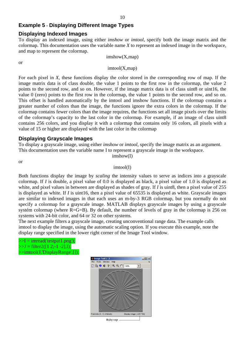
Both functions display the image by scaling the intensity values to serve as indices into a grayscale colormap. If I is double, a pixel value of 0.0 is displayed as black, a pixel value of 1.0 is displayed as white, and pixel values in between are displayed as shades of gray. If I is uint8, then a pixel value of 255 is displayed as white. If I is uint16, then a pixel value of 65535 is displayed as white. Grayscale images are similar to indexed images in that each uses an m-by-3 RGB colormap, but you normally do not specify a colormap for a grayscale image. MATLAB displays grayscale images by using a grayscale systém colormap (where R=G=B). By default, the number of levels of gray in the colormap is 256 on systems with 24-bit color, and 64 or 32 on other systems. The next example filters a grayscale image, creating unconventional range data. The example calls imtool to display the image, using the automatic scaling option. If you execute this example, note the display range specified in the lower right corner of the Image Tool window.

>>I = imread('testpat1.png'); >>J = filter2([1 2;-1 -2],I); >>imtool(J,'DisplayRange',[]);

11Displaying Binary Images In MATLAB, a binary image is of class logical. Binary images contain only 0’s and 1’s. Pixels with the value 0 are displayed as black; pixels with the value 1 are displayed as white. For example, this code reads a binary image into the MATLAB workspace and then displays the image. This documentation uses the variable name BW to represent a binary image in the workspace

>>BW = imread('circles.png'); >>imshow(BW) or >>imtool(BW)

Changing the Display Colors of a Binary Image - You might prefer to invert binary images when you display them, so that 0 values are displayed as white and 1 values are displayed as black. To do this, use the NOT (~) operator in MATLAB. (In this figure, a box is drawn around the image to show the image boundary.) For example: >>imshow(~BW) or >>imtool(~BW)

You can also display a binary image using the indexed image colormap syntax. For example, the following command specifies a two-row colormap that displays 0’s as red and 1’s as blue.

>>imshow(BW,[1 0 0; 0 0 1]) or >>imtool(BW,[1 0 0; 0 0 1])

Displaying Truecolor Images Truecolor images, also called RGB images, represent color values directly, rather than through a colormap. A truecolor image is an m-by-n-by-3 array. For each pixel (r,c) in the image, the color is represented by the triplet (r,c,1:3). To display a truecolor image, using either imshow or imtool, specify the image matrix as an argument. For example, this code reads a truecolor image into the MATLAB workspace and then displays the image. This documentation uses the variable name RGB to represent a truecolor image in the workspace

>>RGB = imread(`peppers.png'); >>imshow(RGB) or

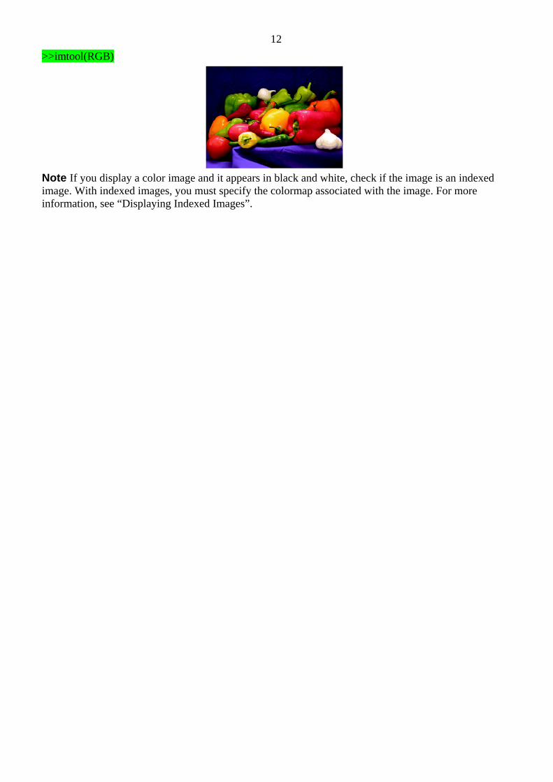
12>>imtool(RGB)

Note If you display a color image and it appears in black and white, check if the image is an indexed image. With indexed images, you must specify the colormap associated with the image. For more information, see “Displaying Indexed Images”.