Embed Size (px)
Citation preview
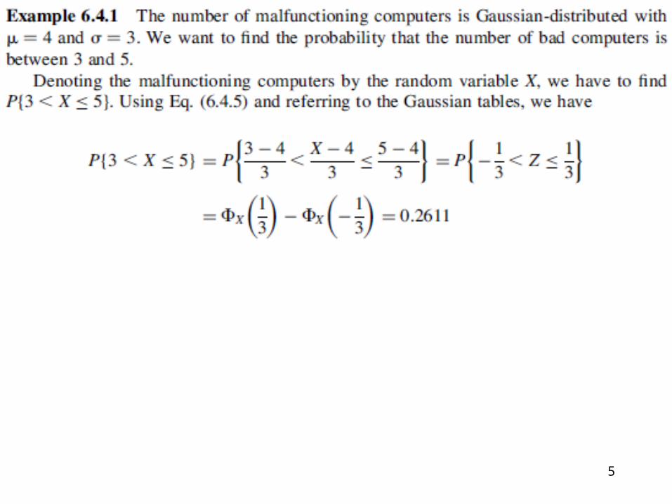
1
Continuous-type random variables
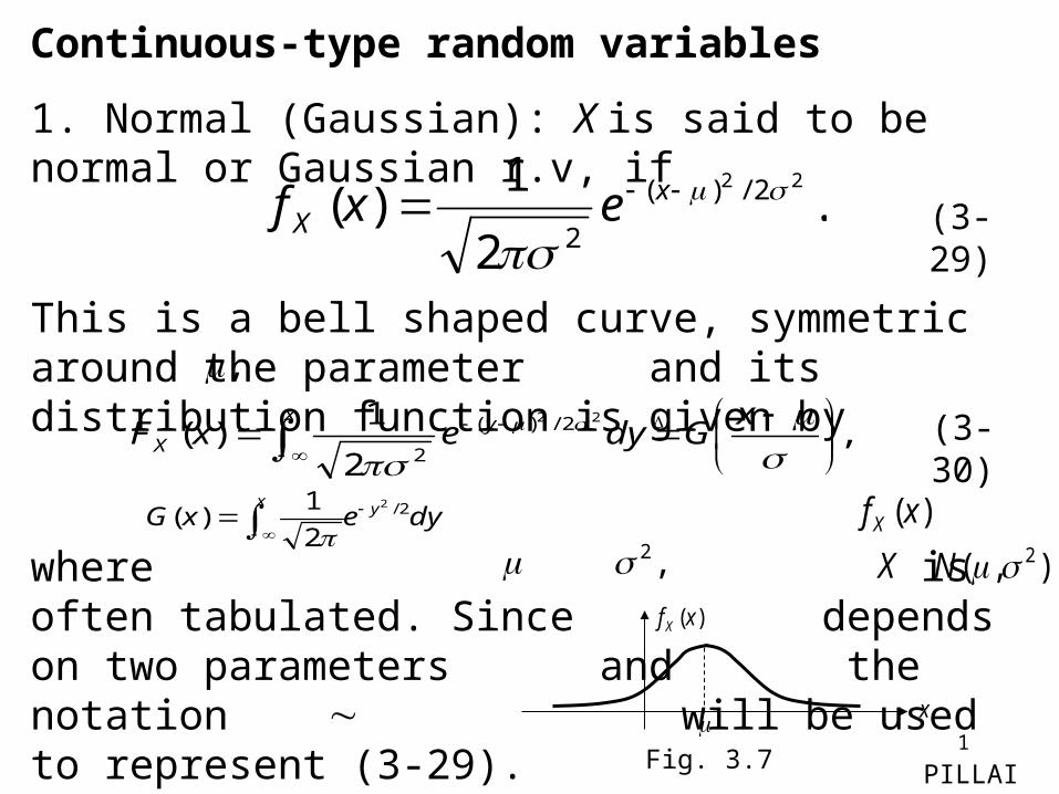
1. Normal (Gaussian): X is said to be normal or Gaussian r.v, if
This is a bell shaped curve, symmetric around the parameter and its distribution function is given by
where is often tabulated. Since depends on two parameters and the notation will be used to represent (3-29).
.2
1)(
22 2/)(
2
x
X exf (3-29)
,
,2
1)(
22 2/)(
2
x y
X
xGdyexF
(3-30)
dyexG yx 2/2
2
1)(
),( 2NX)(xf X
xFig. 3.7
)(xf X
,2
PILLAI
2
3
4
5
6
7
8
9
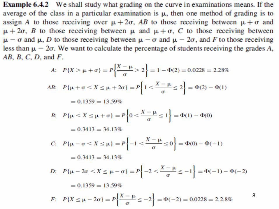
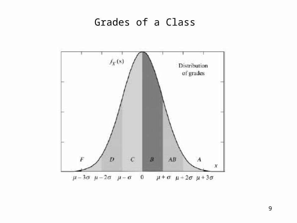
Grades of a Class
10
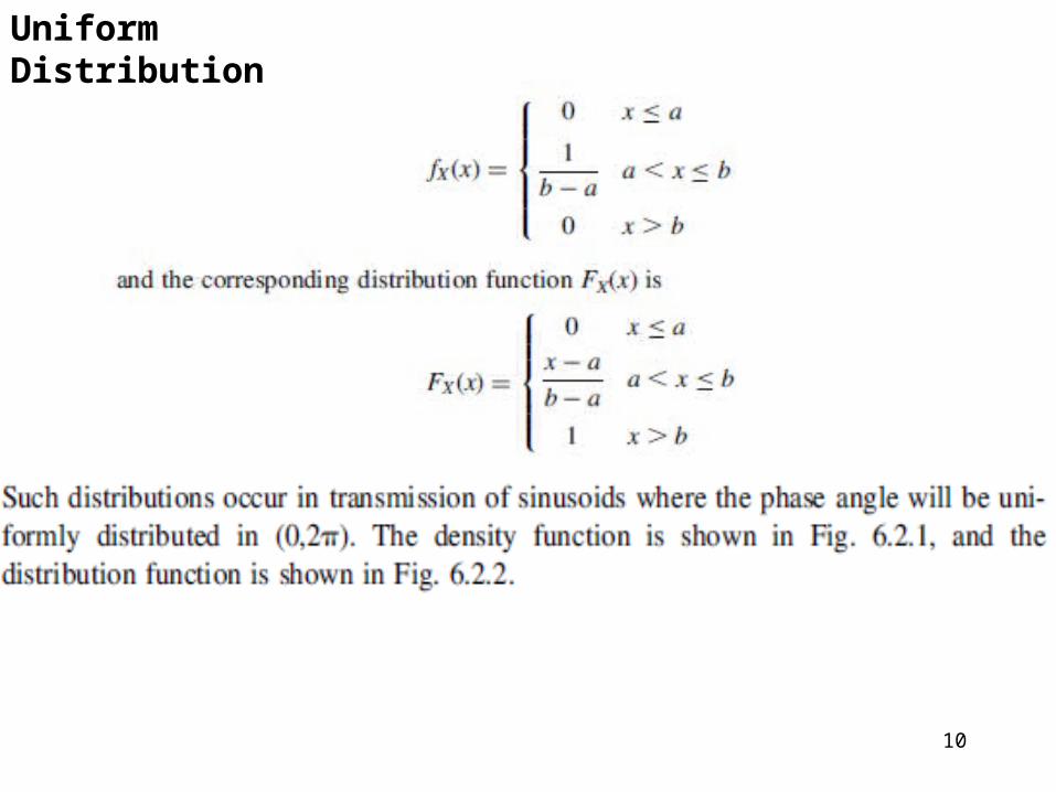
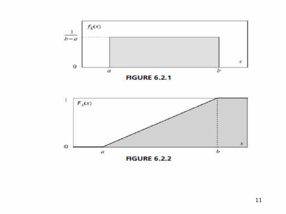
Uniform Distribution
11
12
13
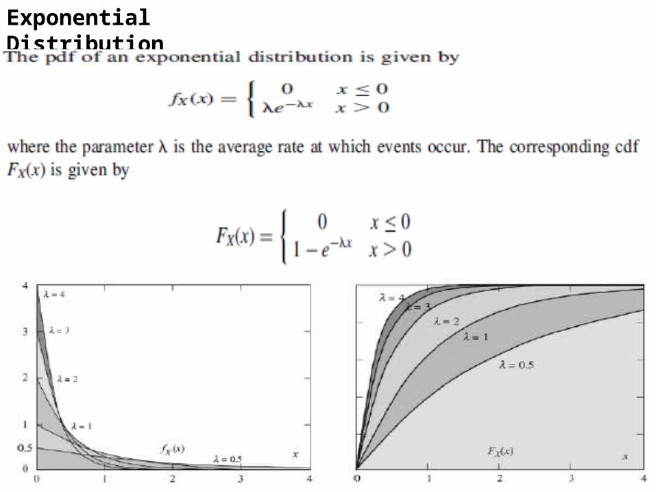
Exponential Distribution
14
15
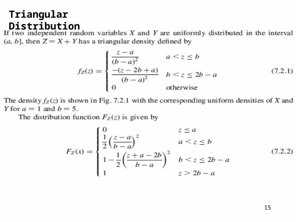
Triangular Distribution
16
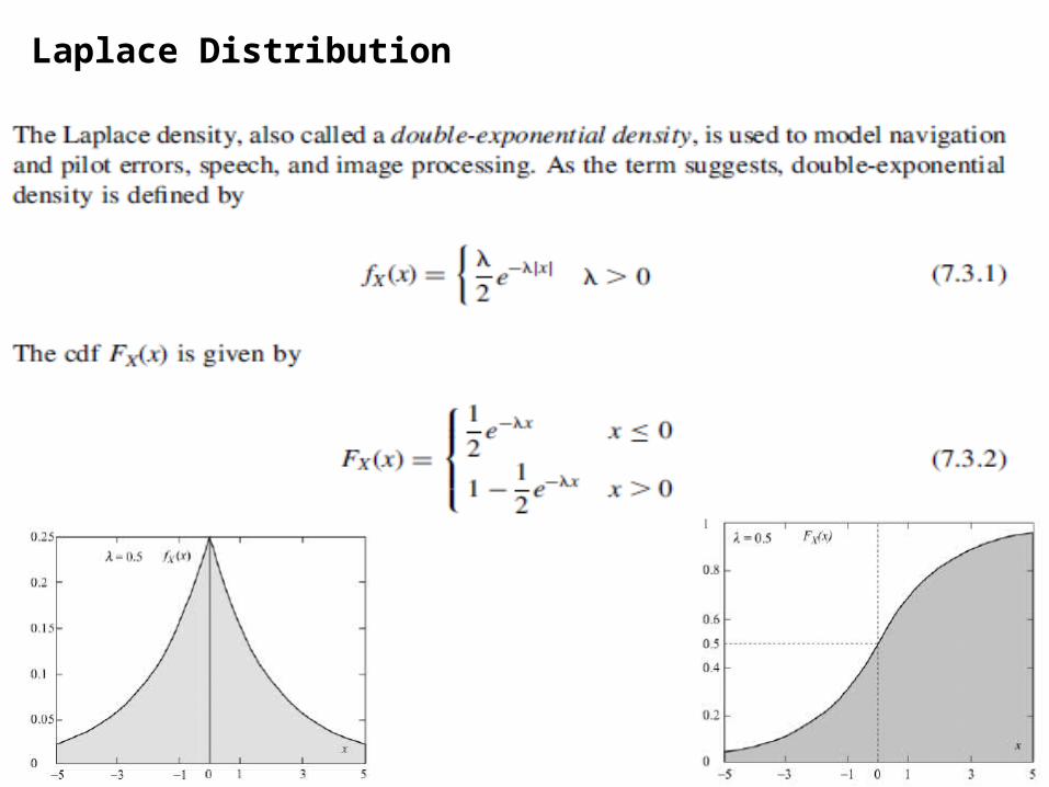
Laplace Distribution
17
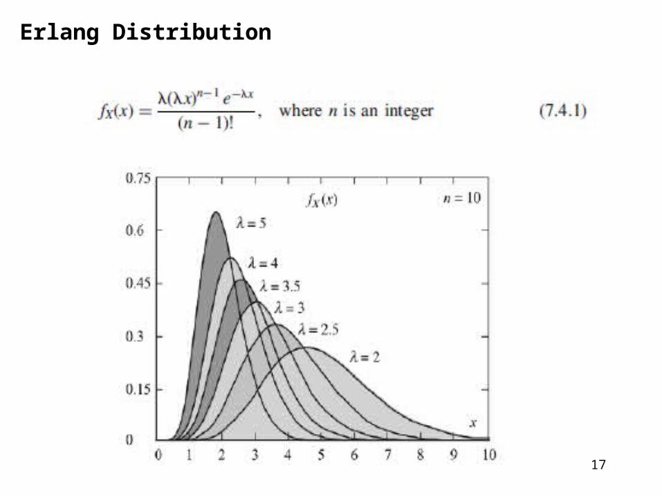
Erlang Distribution
18
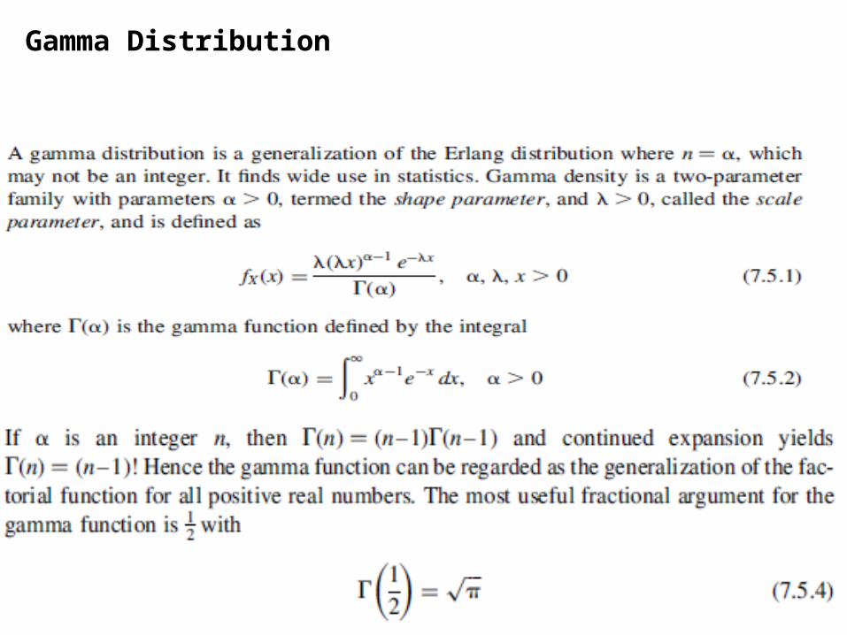
Gamma Distribution
19
20
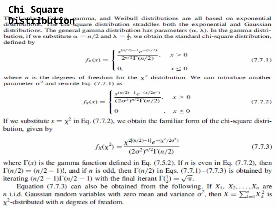
Chi Square Distribution
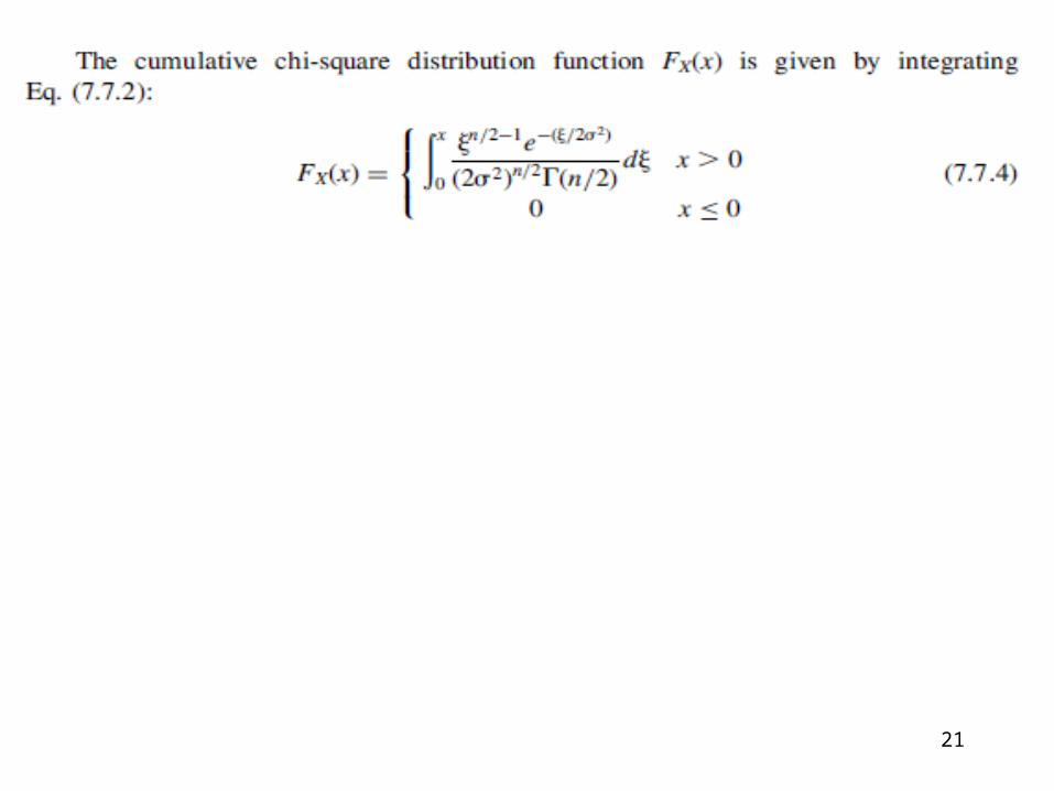
21
22
Discrete-type random variables
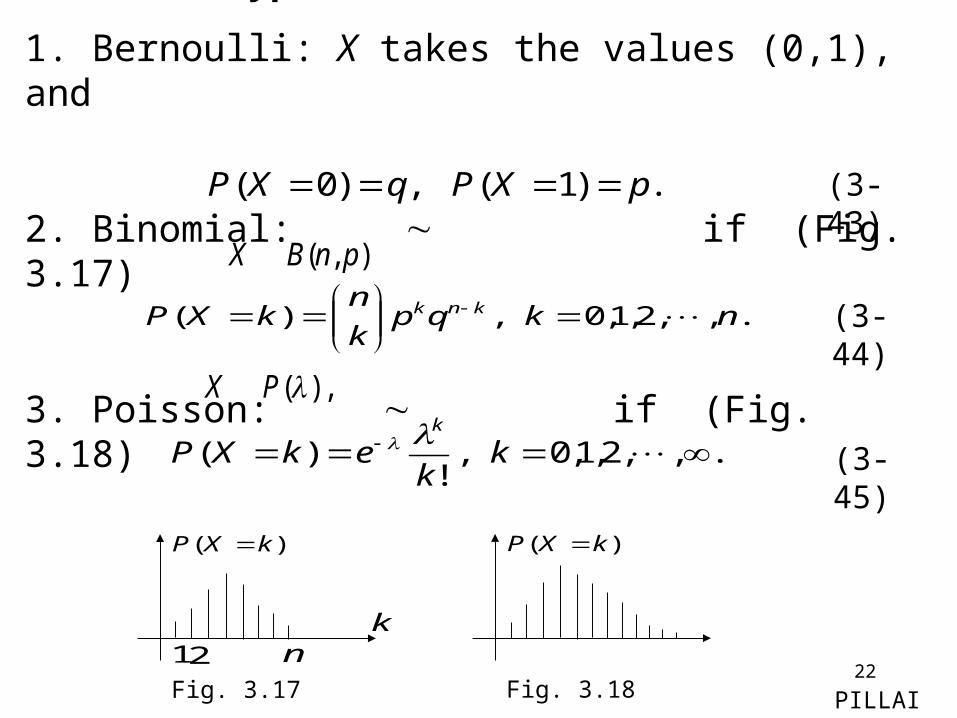
1. Bernoulli: X takes the values (0,1), and
2. Binomial: if (Fig. 3.17)
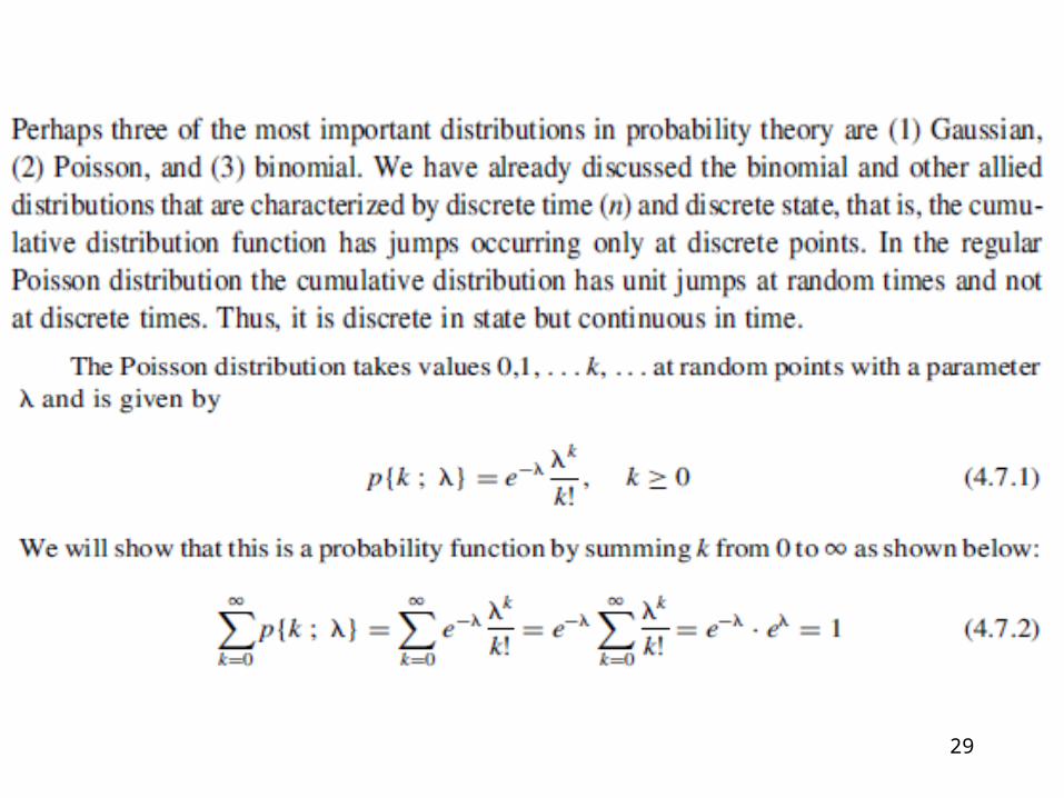
3. Poisson: if (Fig. 3.18)
.)1( ,)0( pXPqXP (3-43)
),,( pnBX
.,,2,1,0 ,)( nkqpk
nkXP knk
(3-44)
, )( PX
.,,2,1,0 ,!
)( kk
ekXPk
(3-45)
k
)( kXP
Fig. 3.17
12 n
)( kXP
Fig. 3.18 PILLAI
23
24
25
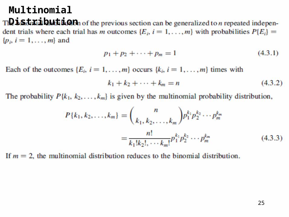
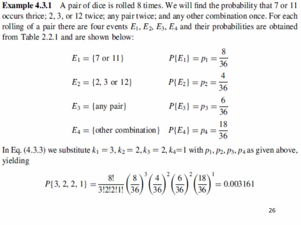
Multinomial Distribution
26
27
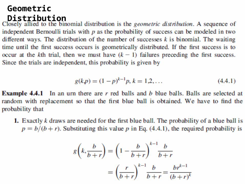
Geometric Distribution
28
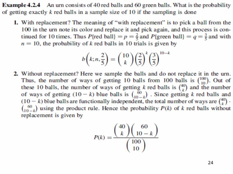
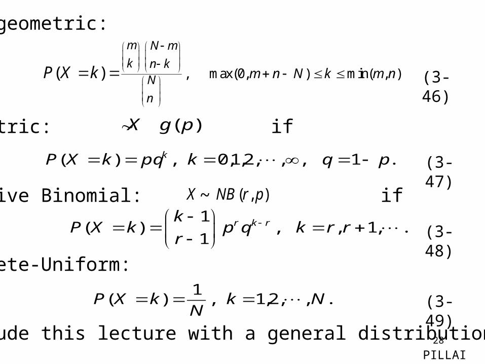
4. Hypergeometric:
5. Geometric: if
6. Negative Binomial: ~ if
7. Discrete-Uniform:
We conclude this lecture with a general distribution duePILLAI
(3-49)
(3-48)
(3-47)
.,,2,1 ,1
)( NkN
kXP
),,( prNBX1
( ) , , 1, .1
r k rkP X k p q k r r
r
.1 ,,,2,1,0 ,)( pqkpqkXP k
)( pgX
, max(0, ) min( , )( )
m N m
k n kN
n
m n N k m nP X k
(3-46)
29
30
31