UNDER THE GUIDANCE OF

Dr. Pitam Singh

DEPARTMENT OF MATHEMATICS

Motilal Nehru National Institute of Technology

Allahabad, Uttar Pradesh -211004

Fuzzy sets were introduced by Lotfi A.Zadeh and Dieter Klaua

in 1965 as an extension of the classical notion of set.

In classical set theory, the

membership of elements in a set is

assessed in binary terms according to a

bivalent condition — an element either

belongs or does not belong to the set.

By contrast, fuzzy set theory permits the gradual assessment of the

membership of elements in a set; this is described with the aid of a

membership function valued in the real unit interval [0, 1].

In the modeling of real world phenomena, often some or

most of the pertinent information may be uncertain. For

example, the precise initial state may not be known or

information about various parameters required as a part of

the model may be imprecise. Many times, the nature of the

uncertainty involved may not be statistical. In such situations

involving uncertainties, Fuzzy deferential equations(FDEs) are

a natural way to model dynamical systems. Here, we are

interested in issues concerning Fuzzy Initial Value Problems

(FIVP).

Why we study??

Fuzzy Initial Value problem

Consider the initial value problem (IVP for

short) for the fuzzy differential equation

𝑢′ = 𝑓 𝑡, 𝑢 , 𝑢 𝑡0 = 𝑢0 ; 𝑡0 ≥ 0

Where 𝑓: 𝐽 × 𝐸𝑛 → 𝐸𝑛; 𝐽 = 𝑡0, 𝑡0 + 𝑎 , 𝑎 >0 and

𝐸𝑛, 𝑑 is a n-dimentional fuzzy metric space.

Let us first note that a mapping 𝑢: 𝐽 → 𝐸𝑛 is a

solution of the IVP

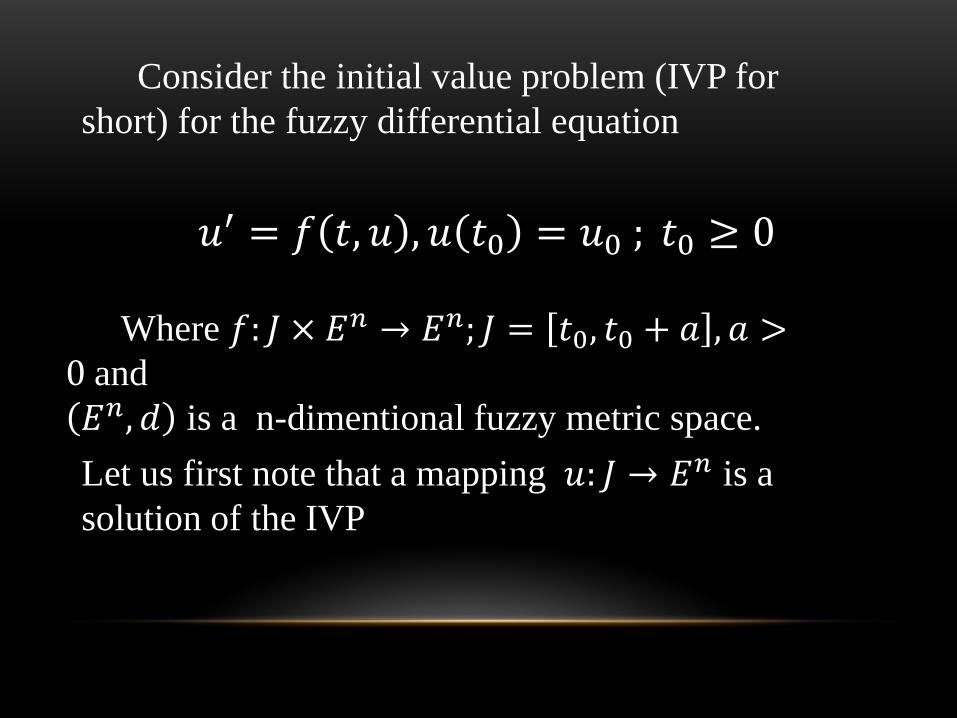
Let 𝑥, 𝑦 ∈ 𝐸. If there exists 𝑧 ∈ 𝐸 such that 𝑥 = 𝑦 + 𝑧 ; then 𝑧 is called the H-difference of x and y and it is denoted

by 𝑥 ⊖ 𝑦.

Here ⊖ sign stands always for H-difference and let us

remark that x⊖ y ≠ x + (−1)y. Usually we denote 𝑥 + (−)𝑦 by 𝑥 − 𝑦 ; while

𝑥 ⊖ 𝑦 stands for the H-difference.

Let 𝑓: (𝑎, 𝑏) → 𝐸 and 𝑥0 ∈ ,𝑎, 𝑏-.We say that 𝑓is strongly generalized

differentiable at 𝑥0 ,if there exit an element 𝑓′(𝑥0) ∈ 𝐸,such that

1) ∀ 𝑕 > 0 sufficiently small ,∃ 𝑓 𝑥0 + 𝑕 ⊖ 𝑓 𝑥0 , 𝑓 𝑥0 ⊖𝑓 𝑥0 − 𝑕 and the

limits (in (𝐸, 𝑑))

limℎ→0

𝑓 𝑥0 + 𝑕 ⊖ 𝑓 𝑥0𝑕

= limℎ→0

𝑓 𝑥0 ⊖𝑓 𝑥0 − 𝑕

𝑕= 𝑓′(𝑥0)

2) ∀ 𝑕 > 0 sufficiently small ,∃ 𝑓 𝑥0 ⊖𝑓 𝑥0 + 𝑕 , 𝑓 𝑥0 − 𝑕 ⊖ 𝑓 𝑥0 and the

limits (in (𝐸, 𝑑))

limℎ→0

𝑓 𝑥0 ⊖𝑓 𝑥0 + 𝑕

−𝑕= limℎ→0

𝑓 𝑥0 − 𝑕 ⊖ 𝑓 𝑥0−𝑕

= 𝑓′(𝑥0)

OR

OR

Let 𝑓: (𝑎, 𝑏) → 𝐸 and 𝑥0 ∈ ,𝑎, 𝑏-.We say that 𝑓is strongly generalized

differentiable at 𝑥0 ,if there exit an element 𝑓′(𝑥0) ∈ 𝐸,such that

Let 𝑓: (𝑎, 𝑏) → 𝐸 and 𝑥0 ∈ ,𝑎, 𝑏-.We say that 𝑓is strongly generalized

differentiable at 𝑥0 ,if there exit an element 𝑓′(𝑥0) ∈ 𝐸,such that

3) ∀ 𝑕 > 0 sufficiently small ,∃ 𝑓 𝑥0 + 𝑕 ⊖ 𝑓 𝑥0 , 𝑓 𝑥0 − 𝑕 ⊖ 𝑓 𝑥0 and the

limits (in (𝐸, 𝑑))

limℎ→0

𝑓 𝑥0 + 𝑕 ⊖ 𝑓 𝑥0𝑕

= limℎ→0

𝑓 𝑥0 − 𝑕 ⊖ 𝑓 𝑥0−𝑕

= 𝑓′(𝑥0)

4) ∀ 𝑕 > 0 sufficiently small ,∃ 𝑓 𝑥0 ⊖𝑓 𝑥0 + 𝑕 , 𝑓 𝑥0 − 𝑕 ⊖ 𝑓 𝑥0 and the

limits (in (𝐸, 𝑑))

limℎ→0

𝑓 𝑥0 ⊖𝑓 𝑥0 + 𝑕

𝑕= limℎ→0

𝑓 𝑥0 ⊖𝑓 𝑥0 − 𝑕

−𝑕= 𝑓′(𝑥0)

OR

A function that is strongly generalized

differentiable as in cases (i) and (ii) , will be referred

as (i)-differentiable or as (ii)-differentiable,

respectively.

As for cases (iii) and (iv), a function may be

differentiable as in (iii) or (iv) only on a discrete set

of points (where differentiability switches between

cases (i) and (ii)).

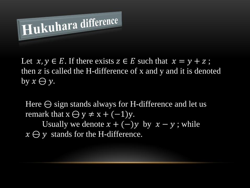
Theorem: If 𝒇 𝒕 = *𝒙 𝒕 , 𝒚 𝒕 , 𝒛(𝒕)+ is triangular number valued function,

then

a) If 𝒇 is (i)-differentiable (Hukuhara differentiable) then 𝒇′ = (𝒙′, 𝒚′, 𝒛′). b)If 𝒇 is (ii)-differentiable (Hukuhara differentiable) then 𝒇′= (𝒛′, 𝒚′, 𝒙′).

Proof:

The proof of (b) is as follows. Let us suppose that the H-difference exists.

Then, by direct computation we get

𝒍𝒊𝒎𝒉→𝟎

𝒇 𝒕 ⊖ 𝒇 𝒕 + 𝒉

−𝒉= 𝒍𝒊𝒎𝒉→𝟎

𝒙 𝒕 − 𝒙 𝒕 + 𝒉 , 𝒚 𝒕 − 𝒚 𝒕 + 𝒉 , 𝒛 𝒕 − 𝒛 𝒕 + 𝒉

−𝒉

= 𝒍𝒊𝒎𝒉→𝟎

𝒛 𝒕 −𝒛 𝒕 + 𝒉

−𝒉,𝒚 𝒕 −𝒚 𝒕+𝒉

−𝒉,𝒙 𝒕 −𝒙 𝒕 + 𝒉

−𝒉= (𝒛′, 𝒚′, 𝒙′)

Similarly, 𝒍𝒊𝒎𝒉→𝟎

𝒇 𝒕−𝒉 ⊖𝒇 𝒕

−𝒉= (𝒛′, 𝒚′, 𝒙′)

In the following equivalent crisp differential equations are considered

𝒖′ = −𝒖+ 𝝈 𝒕 , 𝒖′ − 𝝈 𝒕 = −𝒖 𝒂𝒏𝒅 𝒖′ + 𝒖 = 𝝈 𝒕 , 𝒖 𝟎 = 𝒖𝟎

When these equations are fuzzified we get three different

fuzzy differential equations and exhibit very different behaviors.

In this section, we begin with the inequivalent homogeneous

FIVPs, and then contrast their behavior with the behavior of the

solutions of the corresponding nonhomogeneous FDEs. In this

section we use exclusively the Hukuhara type differentiability.

We discuss the above problem with the help of

next examples

Let us consider FIVP : 𝒖′ = −𝒖, 𝒖 𝟎 = (−𝟏, 𝟎, 𝟏)

The solution of this problem is 𝒖(𝒕) = (−𝒆𝒕, 𝟎, 𝒆𝒕).

Its graphical representation is

(i)-differentiability is in fact

Hukuhara differentiability,we

obtain the unstable solution

of this figure.

Let us consider FIVP : 𝒖′ = −𝒖, 𝒖 𝟎 = (−𝟏, 𝟎, 𝟏)

Under (ii)-differentiability condition ,

we get the solution 𝑢 𝑡 = (−𝑒−𝑡 , 0, 𝑒−𝑡).

Solution of above equation under (ii)-differentiability is represented in the

below figure.

Now, if we consider the corresponding equivalent

nonhomogeneous FIVP,

1) 𝒖′ + 𝒖 = 𝟐𝒆−𝒕 −𝟏, 𝟎, 𝟏 , 𝒖 𝟎 = (−𝟏, 𝟎, 𝟏)

2) 𝒖′ = −𝒖 + 𝟐𝒆−𝒕 −𝟏, 𝟎, 𝟏 , 𝒖 𝟎 = −𝟏, 𝟎, 𝟏

3) 𝒖′ − 𝟐𝒆−𝒕 −𝟏, 𝟎, 𝟏 = −𝒖, 𝒖 𝟎 = (−𝟏, 𝟎, 𝟏)

1st consider :

z

' 2 ; (0) 1 ' 0; (0) 0 ' 2 ; (0) 1

( ) (2 1)

2 1,0,1 , 0 1,0,

( ) 0 ( ) (2 1)

( ) [ ( ), ( ), ( )] [ (2 1) ,0, (2 1) ]

1t

t t

t t

t t

for x for y for

x x e x y y y z z e z

x t t e y t z t t e

u t x t y t z t t e

u u e

t

u

e

Its graphical representation is

2nd we consider :

z

' 2 ; (0) 1 ' ; (0) 0 ' 2 ; (0) 1

( ) (2 1) ( ) 0 ( ) (2 1)

( ) [ ( ), ( ), ( )] [

2 1,0,1 , 0

2 ,0,

1,0

2 ], (0, )

,1

t t

t t

t t t t

t

for x for y for

x z e x y y y z x e z

x t t e y t z t t e

u t x t y t z t e e e e

u u u

t

e

Its graphical representation is

z

' 2 ; (0) 1 ' ;

Now consider 3rd equati

(0) 0 ' 2 ; (0) 1

( ) ( ) 0 ( )

( ) [ ( ),

on:

( ), ( )] [ ,0,

2 1,0,1 , 0 1,0,1

]

t t

t t

t t

t

for x for y for

x e z x y y y

u e u u

z e x z

x t e y t z t e

u t x t y t z t e e

but in this case u is not H-differentiable since the H-differences

𝑢(𝑡 + 𝑕) ⊖ 𝑢(𝑡) and 𝑢(𝑡) ⊖ 𝑢(𝑡 − 𝑕) do not exist.

We observe that the solutions of the equations (1) and (2)

behave in quite different ways, as shown in Figures, however these

equations are different fuzzyfications of equivalent crisp ODEs.

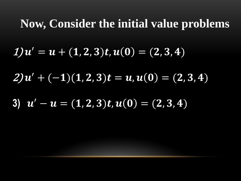
Now, Consider the initial value problems

1)𝒖′ = 𝒖 + (𝟏, 𝟐, 𝟑)𝒕, 𝒖 𝟎 = (𝟐, 𝟑, 𝟒)

2)𝒖′ + (−𝟏)(𝟏, 𝟐, 𝟑)𝒕 = 𝒖, 𝒖 𝟎 = (𝟐, 𝟑, 𝟒)

3) 𝒖′ − 𝒖 = (𝟏, 𝟐, 𝟑)𝒕, 𝒖 𝟎 = (𝟐, 𝟑, 𝟒)

z

' ; (0

Consi

) 2 ' 2 ; (0) 3 ' 3 ; (0) 4

( ) 3 1 ( ) 5 2 2 ( ) 7 3 3

( ) [ ( ), ( ), ( )] [3 1,5 2 2,7 3 3]

der 1st : 1, 2,3 , 0 2,3

,

4

, [0 )

,

t t t

t t t

for x for y for

x x t x y y t y z z t z

x t e t y t e t z t e t

u t x t y t z t e t e t e t

u t u

t

u

Its graphical representation is

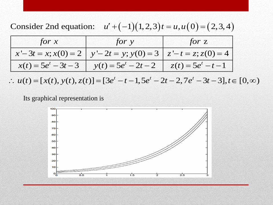
z

' 3 ; (0) 2 ' 2 ; (0) 3 ' ; (0

Consider 2nd equat

) 4

( ) 5 3 3 ( ) 5 2 2 ( ) 5 1

( ) [ ( ), ( ), ( )] [3 1,5 2 2,7 3 3],

ion: 1 1,2,3 , 0 2,3,

[0,

4

)

t t t

t t t

for x for y for

x t x x y t y y z t z z

x t e t y t e t z t e t

u t x t y t z t e t e t e t t

u t u u

Its graphical representation is

z

' ; (0) 2 ' 2 ; (0) 3 ' 3 ; (0) 4

( ) 3.5 3 0

Consider 3rd equation: 1

.5 1 ( ) 5 2 2 ( ) 3.5 0.5

( ) [ ( )

, 2,3 ,

, ( ), ( )] [3.5 3 0.5

0 2,3

1,5

,4

t t t t t

t t t

for x for y for

x z t x y y t y z x t z

x t e t e y t e t z t e t e

u t x t y t z t e t e

u u t u

e

2 2,3.5 0.5 ], (ln 2, )t tt e t e t

Since this is not a solution near the origin we do not consider it a proper solution of

this problem.

∴ 𝑇𝑕𝑒 𝑔𝑟𝑎𝑝𝑕𝑖𝑐𝑎𝑙 𝑟𝑒𝑝𝑟𝑒𝑠𝑒𝑛𝑡𝑎𝑡𝑖𝑜𝑛 𝑜𝑓 𝑡𝑕𝑒 𝑠𝑜𝑙𝑢𝑡𝑖𝑜𝑛𝑠 𝑜𝑓 (1) 𝑎𝑛𝑑 (2) 𝑐𝑎𝑛 𝑏𝑒 𝑠𝑒𝑒𝑛

𝑖𝑛 𝑡𝑕𝑒 𝑎𝑏𝑜𝑣𝑒 𝑓𝑖𝑔𝑒𝑟 𝑟𝑒𝑠𝑝𝑒𝑐𝑡𝑖𝑣𝑒𝑙𝑦. 𝐴𝑔𝑎𝑖𝑛 𝑤𝑒 𝑕𝑎𝑣𝑒 𝑞𝑢𝑖𝑡𝑒 𝑑𝑖𝑓𝑓𝑒𝑟𝑒𝑛𝑡 𝑏𝑒𝑕𝑎𝑣𝑖𝑜𝑟. 𝐼𝑛𝑑𝑒𝑒𝑑, 𝑓𝑜𝑟 𝑡𝑕𝑒 𝑠𝑒𝑐𝑜𝑛𝑑 𝑠𝑜𝑙𝑢𝑡𝑖𝑜𝑛 𝑤𝑒 𝑐𝑜𝑢𝑙𝑑 𝑠𝑎𝑦 𝑡𝑕𝑎𝑡 𝑖𝑡 𝑖𝑠 "𝑟𝑒𝑙𝑎𝑡𝑖𝑣𝑒𝑙𝑦 𝑠𝑡𝑎𝑏𝑙𝑒", 𝑖. 𝑒. 𝑡𝑕𝑒

𝑢𝑛𝑐𝑒𝑟𝑡𝑎𝑖𝑛𝑡𝑦 𝑖𝑠 𝑞𝑢𝑖𝑡𝑒 𝑠𝑚𝑎𝑙𝑙 𝑤. 𝑟. 𝑡. 𝑡𝑕𝑒 𝑐𝑜𝑟𝑒 𝑓𝑜𝑟 𝑙𝑎𝑟𝑔𝑒 𝑣𝑎𝑙𝑢𝑒𝑠 𝑜𝑓 𝑡.

A PREY PREDATOR MODEL

WITH

FUZZY INITIAL VALUES

Consider the following prey-predator model with fuzzy initial

values. Before giving a solution of the fuzzy problem we want to

find its crisp solution.

𝑑𝑥

𝑑𝑡= 0.1𝑥 − 0.005𝑥𝑦

𝑑𝑦

𝑑𝑡= −0.4𝑦 + 0.008𝑥𝑦

with initial condition x 0 = 130 , 𝑦(0) = 40

where x(t) and y(t) are the number of preys and predators at time t, respectively.

Crisp solutions for the above problem are given in the

below Figure

Let the initial values be fuzzy i.e 𝑥 0 = 130 𝑎𝑛𝑑 𝑦 0 = 40

and let their 𝛼-level sets be as follows

𝑥(𝛼) = ,130 -𝛼= ,100 + 30𝛼, 160 − 30𝛼- 𝑦 𝛼 = ,40-𝛼= ,20 + 20𝛼, 60 − 20𝛼-

Let the 𝛼-level sets of 𝑥(𝑡, 𝛼) 𝑏𝑒 ,𝑥(𝑡, 𝛼)-𝛼= ,𝑢(𝑡, 𝛼), 𝑣(𝑡, 𝛼)-, and for simplicity denote them as ,𝑢, 𝑣- , similarly ,𝑦(𝑡, 𝛼)-𝛼=,𝑟(𝑡, 𝛼), 𝑠(𝑡, 𝛼)- = ,𝑟, 𝑠-. Then,

𝑢′, 𝑣′ = 0.1 𝑢, 𝑣 − 0.005 𝑢, 𝑣 . 𝑟, 𝑠

𝑟′, 𝑠′ = −0.4 𝑟, 𝑠 + 0.008 𝑢, 𝑣 . ,𝑟, 𝑠-

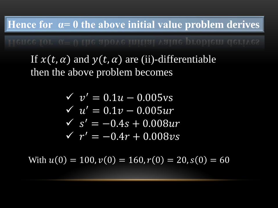
Hence for α= 0 the above initial value problem derives

If 𝑥(𝑡, 𝛼) and 𝑦(𝑡, 𝛼) are (i)-differentiable

then the above problem becomes

𝑢′ = 0.1𝑢 − 0.005vs 𝑣′ = 0.1𝑣 − 0.005𝑢𝑟 𝑟′ = −0.4𝑠 + 0.008𝑢𝑟 𝑠′ = −0.4𝑟 + 0.008𝑣𝑠

With 𝑢 0 = 100, 𝑣 0 = 160, 𝑟 0 = 20, 𝑠 0 = 60

Hence for α= 0 the above initial value problem derives

If 𝑥(𝑡, 𝛼) and 𝑦(𝑡, 𝛼) are (ii)-differentiable

then the above problem becomes

𝑣′ = 0.1𝑢 − 0.005vs 𝑢′ = 0.1𝑣 − 0.005𝑢𝑟 𝑠′ = −0.4𝑠 + 0.008𝑢𝑟 𝑟′ = −0.4𝑟 + 0.008𝑣𝑠

With 𝑢 0 = 100, 𝑣 0 = 160, 𝑟 0 = 20, 𝑠 0 = 60

Now for 𝜶 = 𝟎 the graphical solution of all possible cases are

given below

𝒙(𝒕, 𝜶) and 𝒚(𝒕, 𝜶) are (i)-differentiable

x(t,α) is (ii)-differentiable and y(t,α) is (i)-differentiable

Now if we analyze the above Figure, we

observe that when 𝑥(𝑡, 𝛼) and 𝑦(𝑡, 𝛼) are (ii)-

differentiable the graphical solution is

biologically meaningful

Furthermore the graphical solution is similar with the crisp solution.

when 𝑥(𝑡, 𝛼) and 𝑦(𝑡, 𝛼) are differentiable as (1,1), (1,2), (2,1)

the graphical solutions are incompatible with biological facts.

So we focus on the situation when 𝑥(𝑡, 𝛼) and 𝑦(𝑡, 𝛼) are (ii)-

differentiable. We give the crisp graphical solution and fuzzy

graphical solution when 𝑥(𝑡, 𝛼) and 𝑦(𝑡, 𝛼) are (ii)-differentiable on

the same graph for 𝛼 = 0 and 𝛼 ∈ ,0, 1-. The crisp solution and

fuzzy solution for 𝛼 = 0 are given in the below Figure.

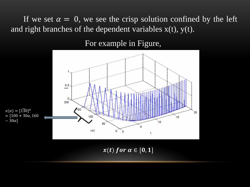
If we set 𝛼 = 0, we see the crisp solution confined by the left

and right branches of the dependent variables x(t), y(t).

For example in Figure,

𝒙(𝒕) 𝒇𝒐𝒓 𝜶 ∈ ,𝟎, 𝟏-

𝑥(𝛼) = ,130 -𝛼

= ,100 + 30𝛼, 160− 30𝛼-

Similarly for, 𝑦 𝑡 𝑓𝑜𝑟 𝛼 ∈ 0, 1

As we see in this example, the uniqueness of the

solution of a fuzzy initial value problem is lost when we

use the strongly generalized derivative concept. This

situation is looked on as a disadvantage. Researchers

can choose the best solution which better reflects the

behavior of the system under consideration, from

multiple solutions.

Surely, the multitude of solutions that are obtained is not really a

disadvantage, since from all the solutions we can find those which better

reflect the behavior of the system under study. This selection of the best

solution in our opinion can be made only from an accurate study of the

physical properties of the system which is studied. This makes it

necessary to study fuzzy differential equations as an independent

discipline, and exploring it further in different directions to facilitate its

use in modeling entirely different physical and engineering problems

satisfactorily. In this sense, the different approaches are complimentary

to each other.