Embed Size (px)
Citation preview

Nonlinear data mining
techniques or clustering to
improve predictions of a
large Brazilian vis-NIR library
Johanna Wetterlind, Bo Stenberg
Suzana Romero Aarújo, José Alexandre Demattê
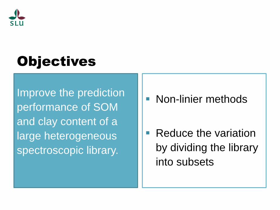
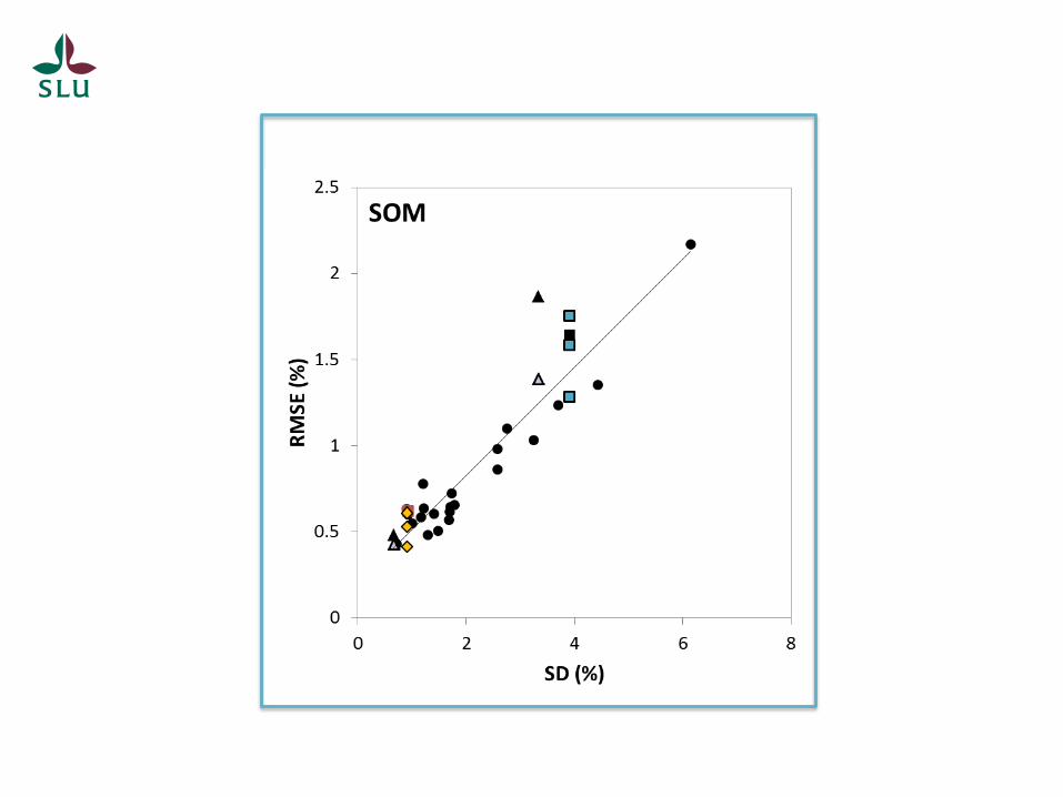
Improve the prediction
performance of SOM
and clay content of a
large heterogeneous
spectroscopic library.
Non-linier methods
Reduce the variation
by dividing the library
into subsets
Objectives
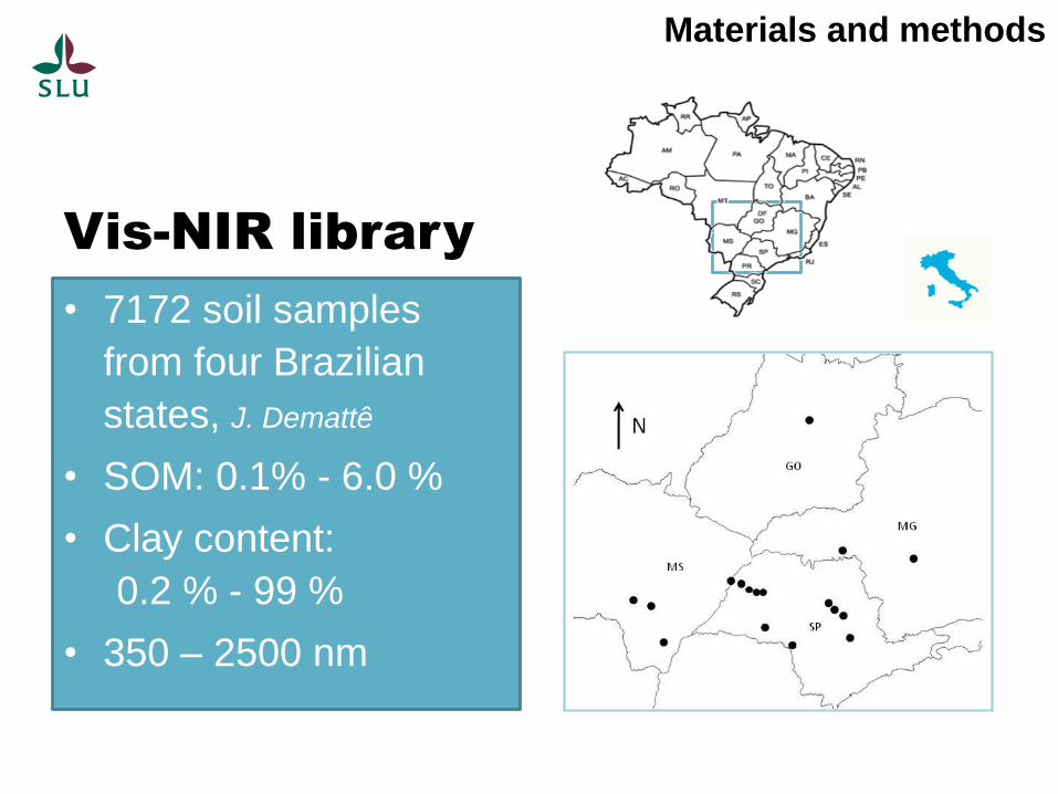
• 7172 soil samples
from four Brazilian
states, J. Demattê
• SOM: 0.1% - 6.0 %
• Clay content:
0.2 % - 99 %
• 350 – 2500 nm
Vis-NIR library
Materials and methods
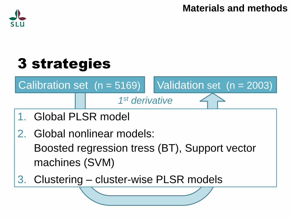
3 strategies
Calibration set (n = 5169) Validation set (n = 2003)
Materials and methods
1. Global PLSR model
2. Global nonlinear models:
Boosted regression tress (BT), Support vector
machines (SVM)
3. Clustering – cluster-wise PLSR models
1st derivative
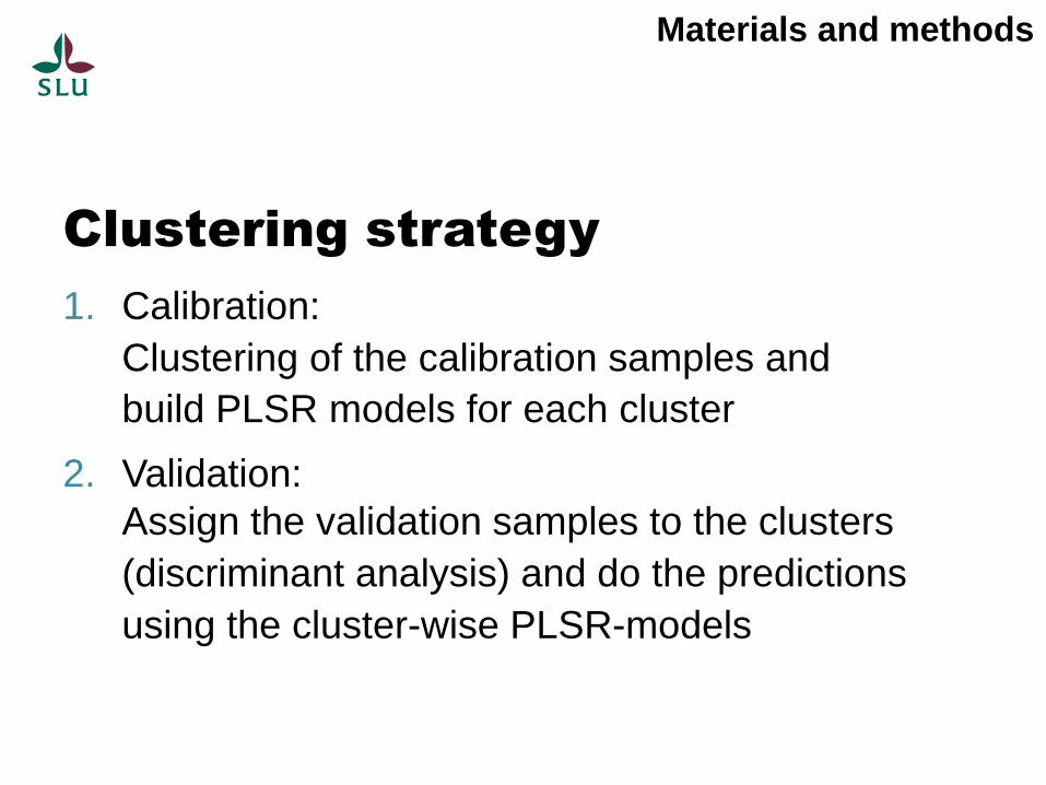
Clustering strategy
1. Calibration:
Clustering of the calibration samples and
build PLSR models for each cluster
2. Validation:
Assign the validation samples to the clusters
(discriminant analysis) and do the predictions
using the cluster-wise PLSR-models
Materials and methods
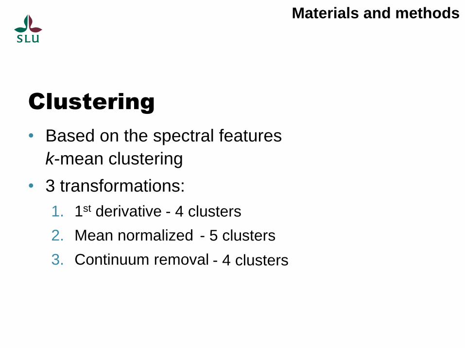
Clustering
• Based on the spectral features
k-mean clustering
• 3 transformations:
1. 1st derivative
2. Mean normalized
3. Continuum removal
Materials and methods
- 4 clusters
- 5 clusters
- 4 clusters
Results
1
0
20
40
60
80
100
120
0 20 40 60 80 100 120
R2 = 0.79RMSE = 11.6
RPD = 2.27
0.0
1.0
2.0
3.0
4.0
5.0
6.0
0.0 1.0 2.0 3.0 4.0 5.0 6.0
R2 = 0.53RMSE = 0.60
RPD = 1.45
0
20
40
60
80
100
120
0 20 40 60 80 100 120
R2 = 0.83RMSE = 10.8
RPD = 2.35
0.0
1.0
2.0
3.0
4.0
5.0
6.0
0.0 1.0 2.0 3.0 4.0 5.0 6.0
R2 = 0.61RMSE = 0.54
RPD = 1.60
0
20
40
60
80
100
120
0 20 40 60 80 100 120
R2 = 0.81RPD = 2.30
RMSE = 11.00
0.0
1.0
2.0
3.0
4.0
5.0
6.0
0.0 1.0 2.0 3.0 4.0 5.0 6.0
R2 = 0.55RMSE = 0.62
RPD = 1.44
Pre
dic
ted O
M, %
Measured Clay, % Measured OM, %
Pre
dic
ted C
lay, %
(a)
(b)
(c)
1
0
20
40
60
80
100
120
0 20 40 60 80 100 120
R2 = 0.79RMSE = 11.6
RPD = 2.27
0.0
1.0
2.0
3.0
4.0
5.0
6.0
0.0 1.0 2.0 3.0 4.0 5.0 6.0
R2 = 0.53RMSE = 0.60
RPD = 1.45
0
20
40
60
80
100
120
0 20 40 60 80 100 120
R2 = 0.83RMSE = 10.8
RPD = 2.35
0.0
1.0
2.0
3.0
4.0
5.0
6.0
0.0 1.0 2.0 3.0 4.0 5.0 6.0
R2 = 0.61RMSE = 0.54
RPD = 1.60
0
20
40
60
80
100
120
0 20 40 60 80 100 120
R2 = 0.81RPD = 2.30
RMSE = 11.00
0.0
1.0
2.0
3.0
4.0
5.0
6.0
0.0 1.0 2.0 3.0 4.0 5.0 6.0
R2 = 0.55RMSE = 0.62
RPD = 1.44
Pre
dic
ted
OM
, %
Measured Clay, % Measured OM, %
Pre
dic
ted
Cla
y,
%
(a)
(b)
(c)
1
0
20
40
60
80
100
120
0 20 40 60 80 100 120
R2 = 0.79RMSE = 11.6
RPD = 2.27
0.0
1.0
2.0
3.0
4.0
5.0
6.0
0.0 1.0 2.0 3.0 4.0 5.0 6.0
R2 = 0.53RMSE = 0.60
RPD = 1.45
0
20
40
60
80
100
120
0 20 40 60 80 100 120
R2 = 0.83RMSE = 10.8
RPD = 2.35
0.0
1.0
2.0
3.0
4.0
5.0
6.0
0.0 1.0 2.0 3.0 4.0 5.0 6.0
R2 = 0.61RMSE = 0.54
RPD = 1.60
0
20
40
60
80
100
120
0 20 40 60 80 100 120
R2 = 0.81RPD = 2.30
RMSE = 11.00
0.0
1.0
2.0
3.0
4.0
5.0
6.0
0.0 1.0 2.0 3.0 4.0 5.0 6.0
R2 = 0.55RMSE = 0.62
RPD = 1.44
Pre
dic
ted O
M, %
Measured Clay, % Measured OM, %
Pre
dic
ted C
lay, %
(a)
(b)
(c)
1
0
20
40
60
80
100
120
0 20 40 60 80 100 120
R2 = 0.79RMSE = 11.6
RPD = 2.27
0.0
1.0
2.0
3.0
4.0
5.0
6.0
0.0 1.0 2.0 3.0 4.0 5.0 6.0
R2 = 0.53RMSE = 0.60
RPD = 1.45
0
20
40
60
80
100
120
0 20 40 60 80 100 120
R2 = 0.83RMSE = 10.8
RPD = 2.35
0.0
1.0
2.0
3.0
4.0
5.0
6.0
0.0 1.0 2.0 3.0 4.0 5.0 6.0
R2 = 0.61RMSE = 0.54
RPD = 1.60
0
20
40
60
80
100
120
0 20 40 60 80 100 120
R2 = 0.81RPD = 2.30
RMSE = 11.00
0.0
1.0
2.0
3.0
4.0
5.0
6.0
0.0 1.0 2.0 3.0 4.0 5.0 6.0
R2 = 0.55RMSE = 0.62
RPD = 1.44
Pre
dic
ted
OM
, %
Measured Clay, % Measured OM, %
Pre
dic
ted
Cla
y,
%
(a)
(b)
(c)
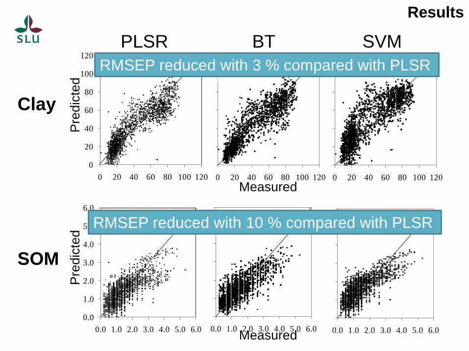
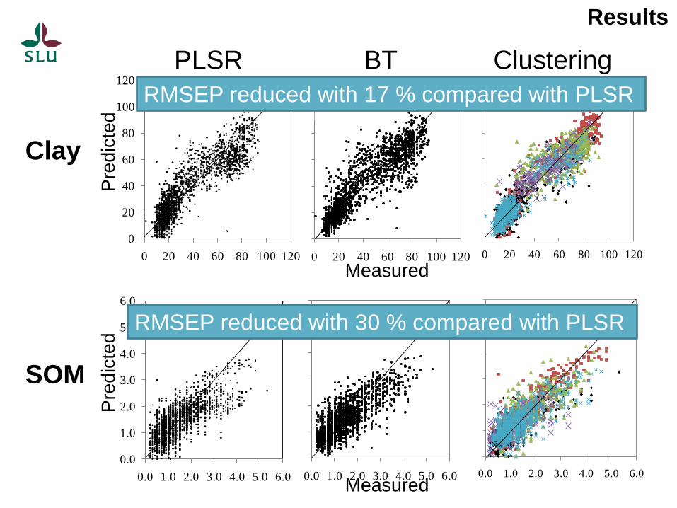
RMSEP = 11.0 %RMSEP = 11.6 % RMSEP = 10.8 %
RMSEP = 0.60 % RMSEP = 0.54 % RMSEP = 0.62 %
PLSR BT SVM
Measured
Measured
Pre
dic
ted
Pre
dic
ted
Clay
SOM
RMSEP reduced with 3 % compared with PLSR
RMSEP reduced with 10 % compared with PLSR
0.0
1.0
2.0
3.0
4.0
5.0
6.0
0.0 1.0 2.0 3.0 4.0 5.0 6.0
R2 = 0.60RMSE = 0.42
RPD = 2.07
Results
1
0
20
40
60
80
100
120
0 20 40 60 80 100 120
R2 = 0.79RMSE = 11.6
RPD = 2.27
0.0
1.0
2.0
3.0
4.0
5.0
6.0
0.0 1.0 2.0 3.0 4.0 5.0 6.0
R2 = 0.53RMSE = 0.60
RPD = 1.45
0
20
40
60
80
100
120
0 20 40 60 80 100 120
R2 = 0.83RMSE = 10.8
RPD = 2.35
0.0
1.0
2.0
3.0
4.0
5.0
6.0
0.0 1.0 2.0 3.0 4.0 5.0 6.0
R2 = 0.61RMSE = 0.54
RPD = 1.60
0
20
40
60
80
100
120
0 20 40 60 80 100 120
R2 = 0.81RPD = 2.30
RMSE = 11.00
0.0
1.0
2.0
3.0
4.0
5.0
6.0
0.0 1.0 2.0 3.0 4.0 5.0 6.0
R2 = 0.55RMSE = 0.62
RPD = 1.44
Pre
dic
ted
OM
, %
Measured Clay, % Measured OM, %
Pre
dic
ted
Cla
y,
%
(a)
(b)
(c)
1
0
20
40
60
80
100
120
0 20 40 60 80 100 120
R2 = 0.79RMSE = 11.6
RPD = 2.27
0.0
1.0
2.0
3.0
4.0
5.0
6.0
0.0 1.0 2.0 3.0 4.0 5.0 6.0
R2 = 0.53RMSE = 0.60
RPD = 1.45
0
20
40
60
80
100
120
0 20 40 60 80 100 120
R2 = 0.83RMSE = 10.8
RPD = 2.35
0.0
1.0
2.0
3.0
4.0
5.0
6.0
0.0 1.0 2.0 3.0 4.0 5.0 6.0
R2 = 0.61RMSE = 0.54
RPD = 1.60
0
20
40
60
80
100
120
0 20 40 60 80 100 120
R2 = 0.81RPD = 2.30
RMSE = 11.00
0.0
1.0
2.0
3.0
4.0
5.0
6.0
0.0 1.0 2.0 3.0 4.0 5.0 6.0
R2 = 0.55RMSE = 0.62
RPD = 1.44
Pre
dic
ted O
M, %
Measured Clay, % Measured OM, %
Pre
dic
ted C
lay, %
(a)
(b)
(c)
1
0
20
40
60
80
100
120
0 20 40 60 80 100 120
R2 = 0.79RMSE = 11.6
RPD = 2.27
0.0
1.0
2.0
3.0
4.0
5.0
6.0
0.0 1.0 2.0 3.0 4.0 5.0 6.0
R2 = 0.53RMSE = 0.60
RPD = 1.45
0
20
40
60
80
100
120
0 20 40 60 80 100 120
R2 = 0.83RMSE = 10.8
RPD = 2.35
0.0
1.0
2.0
3.0
4.0
5.0
6.0
0.0 1.0 2.0 3.0 4.0 5.0 6.0
R2 = 0.61RMSE = 0.54
RPD = 1.60
0
20
40
60
80
100
120
0 20 40 60 80 100 120
R2 = 0.81RPD = 2.30
RMSE = 11.00
0.0
1.0
2.0
3.0
4.0
5.0
6.0
0.0 1.0 2.0 3.0 4.0 5.0 6.0
R2 = 0.55RMSE = 0.62
RPD = 1.44
Pre
dic
ted
OM
, %
Measured Clay, % Measured OM, %
Pre
dic
ted
Cla
y,
%
(a)
(b)
(c)
RMSEP = 11.6 RMSEP = 10.8
RMSEP = 0.60 RMSEP = 0.54 RMSEP = 0.42
PLSR BT
Measured
Measured
Pre
dic
ted
Pre
dic
ted
Clay
SOM
RMSEP reduced with 30 % compared with PLSR
0
20
40
60
80
100
120
0 20 40 60 80 100 120
R2 = 0.87RMSE = 9.3
RPD = 2.7
Clustering
RMSEP = 9.3RMSEP reduced with 17 % compared with PLSR
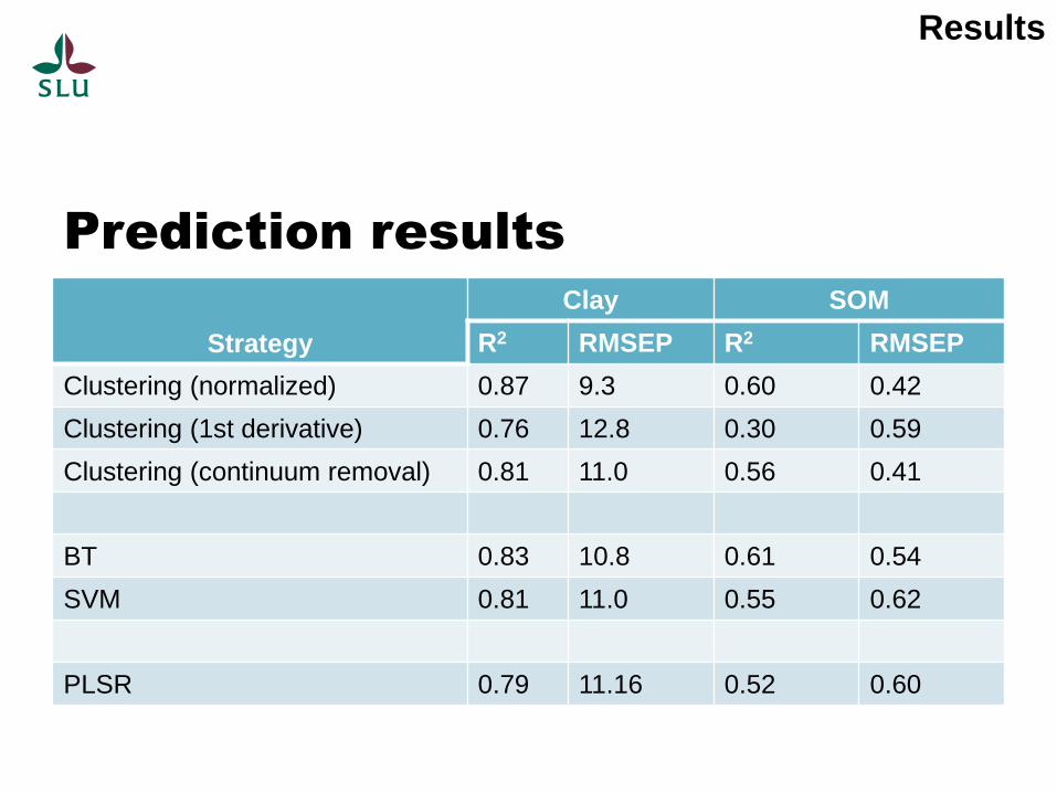
Prediction results
Strategy
Clay SOM
R2 RMSEP R2 RMSEP
Clustering (normalized) 0.87 9.3 0.60 0.42
Clustering (1st derivative) 0.76 12.8 0.30 0.59
Clustering (continuum removal) 0.81 11.0 0.56 0.41
BT 0.83 10.8 0.61 0.54
SVM 0.81 11.0 0.55 0.62
PLSR 0.79 11.16 0.52 0.60
Results
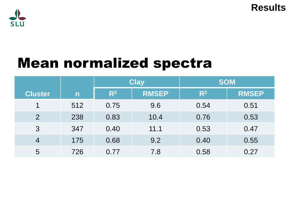
Mean normalized spectra
Cluster n
Clay SOM
R2 RMSEP R2 RMSEP
1 512 0.75 9.6 0.54 0.51
2 238 0.83 10.4 0.76 0.53
3 347 0.40 11.1 0.53 0.47
4 175 0.68 9.2 0.40 0.55
5 726 0.77 7.8 0.58 0.27
Results
Wavelenght/nm
500 750 1000 1250 1500 1750 2000 2250 2500
Continuum
rem
oved s
pectr
a
0.4
0.5
0.6
0.7
0.8
0.9
1.0
1.1
Cluster 1
Cluster 2
Cluster 3
Cluster 4
Cluster 5
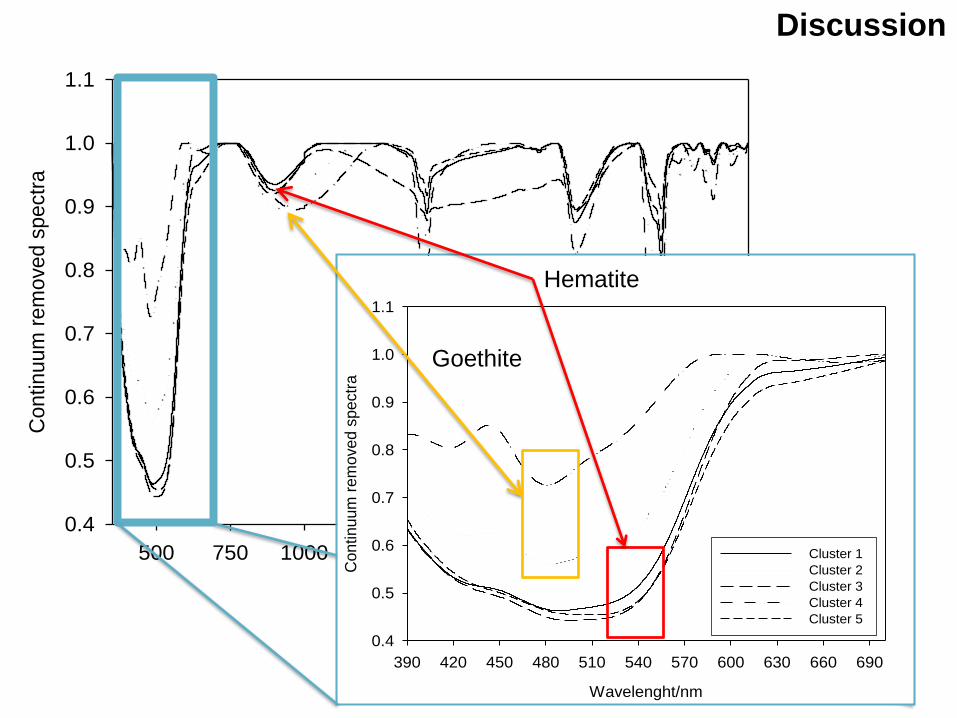
Discussion
Wavelenght/nm
390 420 450 480 510 540 570 600 630 660 690
Co
ntin
uu
m r
em
ove
d s
pe
ctr
a
0.4
0.5
0.6
0.7
0.8
0.9
1.0
1.1
Cluster 1
Cluster 2
Cluster 3
Cluster 4
Cluster 5
Goethite
Hematite
Wavelenght/nm
500 750 1000 1250 1500 1750 2000 2250 2500
Continuum
rem
oved s
pectr
a
0.4
0.5
0.6
0.7
0.8
0.9
1.0
1.1
Cluster 1
Cluster 2
Cluster 3
Cluster 4
Cluster 5
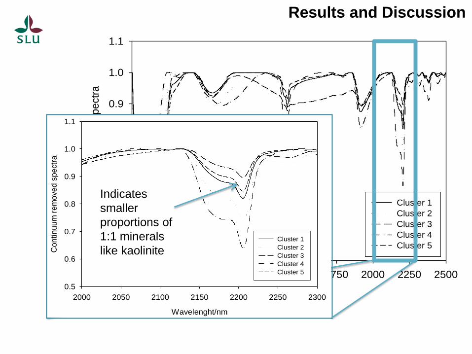
Results and Discussion
Wavelenght/nm
2000 2050 2100 2150 2200 2250 2300
Continuum
rem
oved s
pectr
a
0.5
0.6
0.7
0.8
0.9
1.0
1.1
Cluster 1
Cluster 2
Cluster 3
Cluster 4
Cluster 5
Indicates
smaller
proportions of
1:1 minerals
like kaolinite
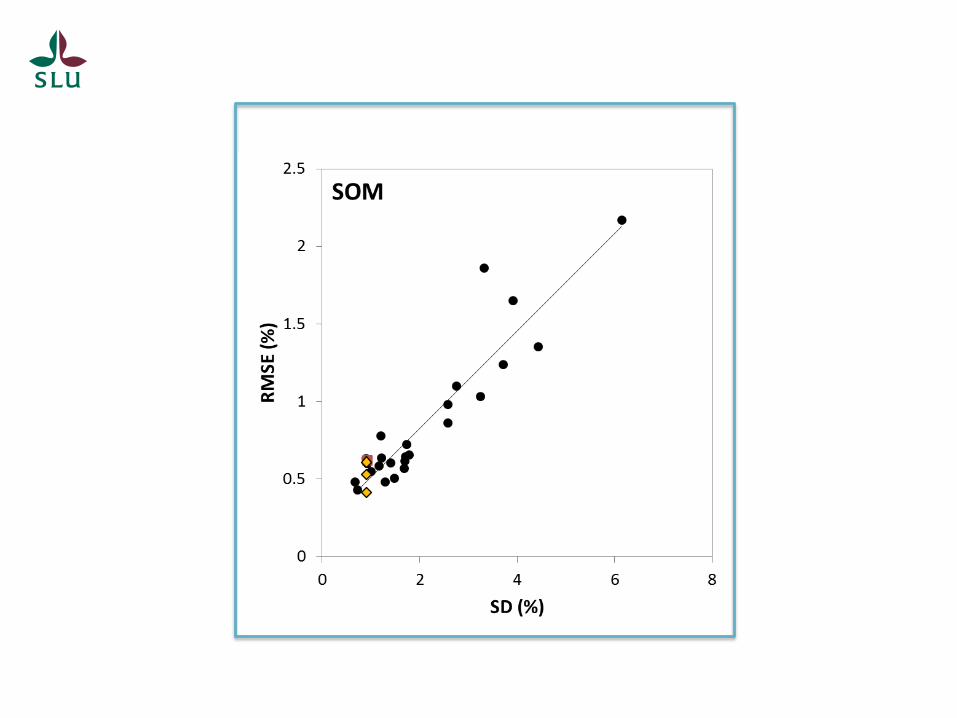
• Reducing the variation in a very dominant feature
such as soil mineralogy within the clusters
enhanced the prediction performance of SOM
content.
• It also improved the predictions of clay content but
not to the same extent.
• Reduce the variation of the soil property of
interest?
Conclusions
• Division of the large library into smaller subsets
based on variation in mean normalized spectra
was the best alternative for both clay and SOM.
• Clustering divided the library into more
mineralogically uniform clusters.
• The additional step of assigning the validation
samples to the right cluster did not add substantial
to the prediction error.