Application of data sparse approximationtechniques for solving SPDE

Alexander Litvinenko

Institut fur Wissenschaftliches Rechnen, Technische Universitat Braunschweig,0531-391-3008, litvinen@tu-bs.de

March 6, 2008

Outline

Problem setup

Karhunen-Loeve expansion

Data Sparse TechniquesFast Fourier Transformation (FFT)Hierarchical MatricesSparse tensor approximation

Applications

Conclusion

Outline

Problem setup

Karhunen-Loeve expansion

Data Sparse TechniquesFast Fourier Transformation (FFT)Hierarchical MatricesSparse tensor approximation

Applications

Conclusion

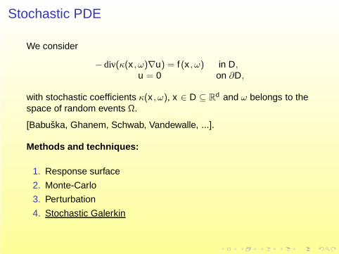
Stochastic PDE

We consider

− div(κ(x , ω)∇u) = f (x , ω) in D,u = 0 on ∂D,

with stochastic coefficients κ(x , ω), x ∈ D ⊆ Rd and ω belongs to the

space of random events Ω.

[Babuska, Ghanem, Schwab, Vandewalle, ...].

Methods and techniques:

1. Response surface

2. Monte-Carlo

3. Perturbation

4. Stochastic Galerkin

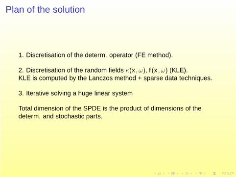
Plan of the solution

1. Discretisation of the determ. operator (FE method).

2. Discretisation of the random fields κ(x , ω), f (x , ω) (KLE).KLE is computed by the Lanczos method + sparse data techniques.

3. Iterative solving a huge linear system

Total dimension of the SPDE is the product of dimensions of thedeterm. and stochastic parts.

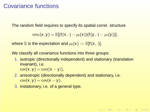
Covariance functions

The random field requires to specify its spatial correl. structure

covf (x , y) = E[(f (x , ·) − µf (x))(f (y , ·) − µf (y))],

where E is the expectation and µf (x) := E[f (x , ·)].

We classify all covariance functions into three groups:

1. isotropic (directionally independent) and stationary (translationinvariant), i.e.cov(x , y) = cov(|x − y |),

2. anisotropic (directionally dependent) and stationary, i.e.cov(x , y) = cov(x − y),

3. instationary, i.e. of a general type.

Outline

Problem setup

Karhunen-Loeve expansion

Data Sparse TechniquesFast Fourier Transformation (FFT)Hierarchical MatricesSparse tensor approximation

Applications

Conclusion

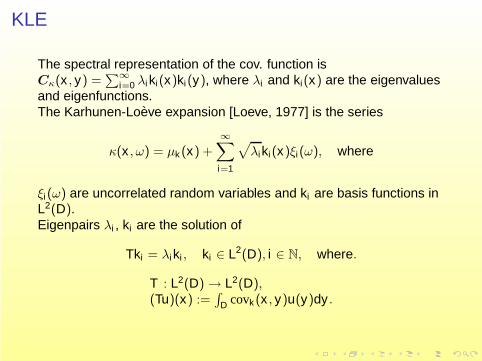
KLE

The spectral representation of the cov. function isCκ(x , y) =

∑∞i=0 λi ki(x)ki(y), where λi and ki(x) are the eigenvalues

and eigenfunctions.The Karhunen-Loeve expansion [Loeve, 1977] is the series

κ(x , ω) = µk (x) +∞∑

i=1

√λiki(x)ξi(ω), where

ξi (ω) are uncorrelated random variables and ki are basis functions inL2(D).Eigenpairs λi , ki are the solution of

Tki = λi ki , ki ∈ L2(D), i ∈ N, where.

T : L2(D) → L2(D),(Tu)(x) :=

∫D covk (x , y)u(y)dy .

Outline

Problem setup

Karhunen-Loeve expansion

Data Sparse TechniquesFast Fourier Transformation (FFT)Hierarchical MatricesSparse tensor approximation

Applications

Conclusion

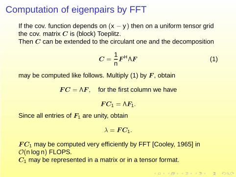
Computation of eigenpairs by FFT

If the cov. function depends on (x − y) then on a uniform tensor gridthe cov. matrix C is (block) Toeplitz.Then C can be extended to the circulant one and the decomposition

C =1n

F HΛF (1)

may be computed like follows. Multiply (1) by F , obtain

FC = ΛF , for the first column we have

FC1 = ΛF1.

Since all entries of F1 are unity, obtain

λ = FC1.

FC1 may be computed very efficiently by FFT [Cooley, 1965] inO(n log n) FLOPS.C1 may be represented in a matrix or in a tensor format.

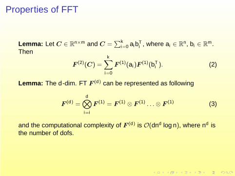
Properties of FFT

Lemma: Let C ∈ Rn×m and C =

∑ki=0 aibT

i , where ai ∈ Rn, bi ∈ R

m.Then

F (2)(C) =

k∑

i=0

F (1)(ai )F(1)(bT

i ). (2)

Lemma: The d-dim. FT F (d) can be represented as following

F (d) =

d⊗

i=i

F (1) = F (1) ⊗ F (1) . . . ⊗ F (1) (3)

and the computational complexity of F (d) is O(dnd log n), where nd isthe number of dofs.

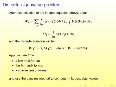
Discrete eigenvalue problem

After discretisation of the integral equation above, obtain

Wij :=∑

k ,m

∫

Dbi(x)bk (x)dxCkm

∫

Dbj(y)bm(y)dy ,

Mij =

∫

Dbi(x)bj (x)dx,

and the discrete equation will be

Wfhℓ = λℓMfh

ℓ , where W := MCM

Approximate C in

a low rank format the H-matrix format a sparse tensor format

and use the Lanczos method to compute m largest eigenvalues.

H-matrix [Hackbusch et al. 99]

25 11

11 20 12

1320 11

9 1613

1320 11

11 20 13

13 3213

13

20 8

10 20 13

13 32 13

1332 13

13 32

13

13

20 11

11 20 13

13 32 13

1320 10

10 20 12

12 3213

1332 13

13 32 13

1332 13

13 32

13

13

20 11

11 20 13

13 32 13

1332 13

13 3213

13

20 9

9 20 13

13 32 13

1332 13

13 32

13

13

32 13

13 32 13

1332 13

13 3213

1332 13

13 32 13

1332 13

13 32

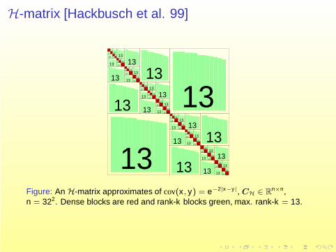
Figure: An H-matrix approximates of cov(x , y) = e−2|x−y|, CH ∈ Rn×n,

n = 322. Dense blocks are red and rank-k blocks green, max. rank-k = 13.

Construction process

H-matrixvertices

finite elements

cluster treeblockcluster tree

admissibilitycondition

admissiblepartitioning

ACAcov. function

a goodpreconditioner

fast arithmetics

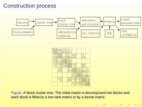
Figure: A block cluster tree. The initial matrix is decomposed into blocks andeach block is filled by a low-rank matrix or by a dense matrix.

H - Matrices

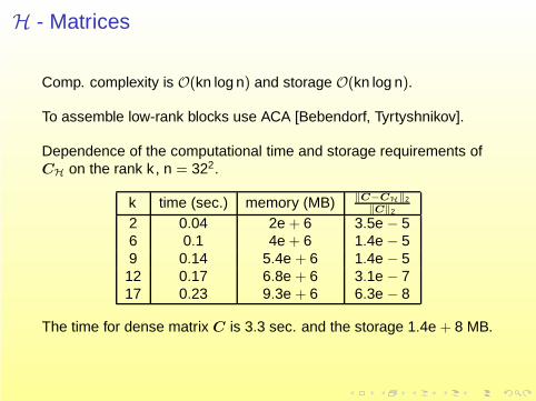
Comp. complexity is O(kn log n) and storage O(kn log n).

To assemble low-rank blocks use ACA [Bebendorf, Tyrtyshnikov].

Dependence of the computational time and storage requirements ofCH on the rank k , n = 322.

k time (sec.) memory (MB) ‖C−CH‖2

‖C‖2

2 0.04 2e + 6 3.5e − 56 0.1 4e + 6 1.4e − 59 0.14 5.4e + 6 1.4e − 512 0.17 6.8e + 6 3.1e − 717 0.23 9.3e + 6 6.3e − 8

The time for dense matrix C is 3.3 sec. and the storage 1.4e + 8 MB.

H - Matrices

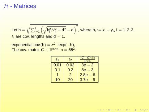
Let h =

√∑2

i=1

(√h2

i /ℓ2i + d2 − d

)2, where hi := xi − yi , i = 1, 2, 3,

ℓi are cov. lengths and d = 1.

exponential cov(h) = σ2 · exp(−h),The cov. matrix C ∈ R

n×n, n = 652.

ℓ1 ℓ2‖C−CH‖2

‖C‖2

0.01 0.02 3e − 20.1 0.2 8e − 31 2 2.8e − 610 20 3.7e − 9

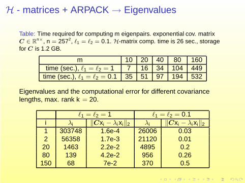
H - matrices + ARPACK → Eigenvalues

Table: Time required for computing m eigenpairs. exponential cov. matrixC ∈ R

n×, n = 2572, ℓ1 = ℓ2 = 0.1. H-matrix comp. time is 26 sec., storagefor C is 1.2 GB.

m 10 20 40 80 160time (sec.), ℓ1 = ℓ2 = 1 7 16 34 104 449

time (sec.), ℓ1 = ℓ2 = 0.1 35 51 97 194 532

Eigenvalues and the computational error for different covariancelengths, max. rank k = 20.

ℓ1 = ℓ2 = 1 ℓ1 = ℓ2 = 0.1i λi ‖Cxi − λi xi‖2 λi ‖Cxi − λi xi‖2

1 303748 1.6e-4 26006 0.032 56358 1.7e-3 21120 0.0120 1463 2.2e-2 4895 0.280 139 4.2e-2 956 0.26150 68 7e-2 370 0.5

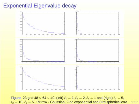
Exponential Eigenvalue decay

0 100 200 300 400 500 600 700 800 900 10000

100

200

300

400

500

600

700

0 100 200 300 400 500 600 700 800 900 10000

1

2

3

4

5

6

7

8

9

10x 10

4

0 100 200 300 400 500 600 700 800 900 10000

200

400

600

800

1000

1200

1400

1600

1800

0 100 200 300 400 500 600 700 800 900 10000

0.5

1

1.5

2

2.5x 10

5

0 100 200 300 400 500 600 700 800 900 10000

50

100

150

0 100 200 300 400 500 600 700 800 900 10000

0.5

1

1.5

2

2.5

3

3.5

4x 10

4

Figure: 23 grid 48 × 64 × 40, (left) ℓ1 = 1, ℓ2 = 2, ℓ3 = 1 and (right) ℓ1 = 5,ℓ2 = 10, ℓ2 = 5. 1st row - Gaussian, 2-nd exponential and 3-rd spherical cov.

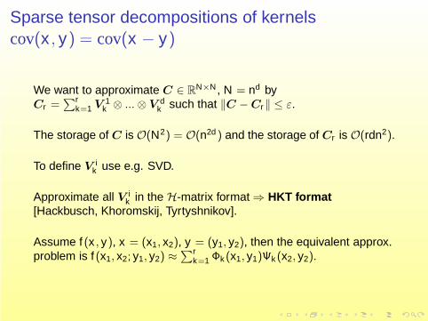
Sparse tensor decompositions of kernelscov(x , y) = cov(x − y)

We want to approximate C ∈ RN×N , N = nd by

Cr =∑r

k=1 V 1k ⊗ ... ⊗ V d

k such that ‖C − Cr‖ ≤ ε.

The storage of C is O(N2) = O(n2d ) and the storage of Cr is O(rdn2).

To define V ik use e.g. SVD.

Approximate all V ik in the H-matrix format ⇒ HKT format

[Hackbusch, Khoromskij, Tyrtyshnikov].

Assume f (x , y), x = (x1, x2), y = (y1, y2), then the equivalent approx.problem is f (x1, x2; y1, y2) ≈

∑rk=1 Φk (x1, y1)Ψk (x2, y2).

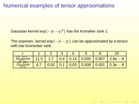
Numerical examples of tensor approximations

Gaussian kernel exp−|x − y |2 has the Kroneker rank 1.

The exponen. kernel exp−|x − y | can be approximated by a tensorwith low Kronecker rank

r 1 2 3 4 5 6 10‖C−Cr‖∞

‖C‖∞11.5 1.7 0.4 0.14 0.035 0.007 2.8e − 8

‖C−Cr‖2

‖C‖26.7 0.52 0.1 0.03 0.008 0.001 5.3e − 9

Outline

Problem setup

Karhunen-Loeve expansion

Data Sparse TechniquesFast Fourier Transformation (FFT)Hierarchical MatricesSparse tensor approximation

Applications

Conclusion

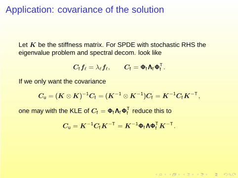
Application: covariance of the solution

Let K be the stiffness matrix. For SPDE with stochastic RHS theeigenvalue problem and spectral decom. look like

Cf fℓ = λℓfℓ, Cf = Φf Λf ΦTf .

If we only want the covariance

Cu = (K ⊗ K)−1Cf = (K−1 ⊗ K−1)Cf = K−1Cf K−T ,

one may with the KLE of Cf = Φf Λf ΦTf reduce this to

Cu = K−1Cf K−T = K−1

Φf ΛΦTf K−T .

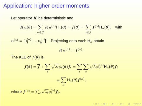
Application: higher order moments

Let operator K be deterministic and

Ku(θ) =∑

α∈J

Ku(α)Hα(θ) = f(θ) =∑

α∈J

f (α)Hα(θ), with

u(α) = [u(α)1 , ..., u(α)

N ]T . Projecting onto each Hα obtain

Ku(α) = f (α).

The KLE of f(θ) is

f(θ) = f +∑

ℓ

√λℓφℓ(θ)fℓ =

∑

ℓ

∑

α

√λℓφ

(α)ℓ Hα(θ)fℓ

=∑

α

Hα(θ)f (α),

where f (α) =∑

ℓ

√λℓφ

(α)ℓ fℓ.

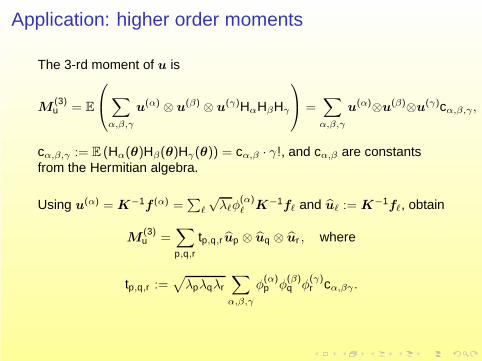
Application: higher order moments

The 3-rd moment of u is

M(3)u = E

∑

α,β,γ

u(α) ⊗ u(β) ⊗ u(γ)HαHβHγ

=∑

α,β,γ

u(α)⊗u(β)⊗u(γ)cα,β,γ ,

cα,β,γ := E (Hα(θ)Hβ(θ)Hγ(θ)) = cα,β · γ!, and cα,β are constantsfrom the Hermitian algebra.

Using u(α) = K−1f (α) =∑

ℓ

√λℓφ

(α)ℓ K−1fℓ and uℓ := K−1fℓ, obtain

M(3)u =

∑

p,q,r

tp,q,r up ⊗ uq ⊗ ur , where

tp,q,r :=√

λpλqλr

∑

α,β,γ

φ(α)p φ

(β)q φ

(γ)r cα,βγ .

Outline

Problem setup

Karhunen-Loeve expansion

Data Sparse TechniquesFast Fourier Transformation (FFT)Hierarchical MatricesSparse tensor approximation

Applications

Conclusion

Conclusion

Covariance matrices allow data sparse approximations. Application of H-matrices

extend the class of covariance functions to work with, allows non-regular discretisations of the cov. function on large

spatial grids.

Application of sparse tensor product allows computation of k -thmoments.

Plans for Feature

1. Apply H-matrix - ARPACK technique for solving SPDEs [M.Krosche’s software]

2. Further research how to apply sparse KLE for computingmoments and functionals of the solution [DFG]

3. Implement sparse tensor vector product for the Lanczos method[MPI Leipzig]

Thank you for your attention!

Questions?