Embed Size (px)
Citation preview

© The Author 2013. Published by Oxford University Press on behalf of the University of North Carolina at Chapel Hill. All rights reserved. For permissions, please e-mail: [email protected].
Social Forces 92(1) 275–302, September 2013doi: 10.1093/sf/sot069
Advance Access publication on 12 July 2013
This research was supported by grant 1R03HD071129-01A1, “Family Size and Children’s Education in Brazil,” awarded to Letícia J. Marteleto in the Population Research Center at the University of Texas at Austin by the Eunice Kennedy Shriver National Institute of Child Health and Human Development. This research was also supported by grant 5R24 HD042849, “Population Research Center,” awarded to the Population Research Center at the University of Texas at Austin by the Eunice Kennedy Shriver National Institute of Child Health and Human Development. The authors are grateful for the helpful comments and suggestions by Robert Hummer, Kelly Raley, Art Sakamoto, and the participants of the Education and Transitions to Adulthood Group, Population Research Center, University of Texas at Austin.
Family Size, Gender, and Birth Order in Brazil
The Implications of Family Size for Adolescents’ Education and Work in Brazil: Gender and Birth Order Differences
Letícia J. Marteleto, University of Texas at AustinLaetícia R. de Souza, International Policy Centre for Inclusive Growth (IPC–IG)
Numerous studies have found a negative association between family size and children’s outcomes, particularly education. The main theoretical frameworks that explain these negative associations posit that family resources medi-
ate the relationship between family size and children’s outcomes, and children are resource receivers only. However, societies in which adolescents often work inside and outside the household and family resources are transferred unequally undermine these assumptions. We implement a twin birth instrumental variable approach and use the nationally representative 1997–2009 PNAD data to examine the impact of family size on school enrollment, labor force, and household work in Brazil. We propose a framework for understanding the implications of family size when adolescents both receive and provide resources in the family unit and these resources may be provided and/or received unequally depending on gender and birth order. While we find no evi-dence of gender or birth order differences in the effects of family size on education, the results indicate strong gender and birth order differences in adolescents’ contribu-tions to their family units. We discuss the implications of our findings for the life course of adolescents.
IntroductionResearchers have long been interested in the influence of family size1 on chil-dren’s education. Simply put, the classical dilution of resources model theo-rizes that family resources (social, cultural, and financial) are diluted within
Family Size, Gender, and Birth Order in Brazil 275

families that have more children, and therefore the larger the family, the fewer the resources available per child and the worse the outcomes for each child (Blake 1981). In such a framework, family resources are key for understanding the relationship between family size and children’s outcomes such that larger families imply fewer resources per child. The dilution of resources model and most research examining the influence of family size on children’s outcomes assume that children only receive resources; however, children and adolescents are resource providers in many parts of the world. Whether adolescents work inside or outside the household likely varies by family size. In developing coun-tries, combining school and work is often the norm for adolescents (Orazem, Glewwe, and Patrinos 2009), and the provision of resources is part of a dynamic process of intra-family transfers. While there are reports that children receive unequal resources based on gender (Parish and Willis 1993; Yu and Su 2006) and birth order (Black, Devereux, and Salvanes 2005; Conley and Glauber 2006; Chu, Xie, and Yu 2007), research has for the most part overlooked differences in the impact of family size on adolescents’ provision of resources to the family.
The first goal of this paper is therefore to examine whether there is a causal effect of family size on adolescent work in Brazil, in addition to education. To more broadly encompass the reality of adolescents’ welfare in Brazil and most developing countries, we move beyond the more common educational outcomes to include economic and household work performed during adolescence. By doing so, we propose a broader conceptualization of the intra-family transfer of resources than suggested by the dilution of resources framework—including economic and household work—that can be applied to the study of the implica-tions of family size for adolescents’ welfare. Although Brazil has experienced recent increases in adolescent school enrollment levels, a large proportion of adolescents still drop out of school—a life stage with long-range impacts for social stratification later in life—and work. Importantly, examining educational and work outcomes will also provide a more detailed picture of adolescents’ welfare in Brazil and most developing countries, an important counterpoint to the current literature that focuses primarily on the United States or other devel-oped countries.
The second goal of this paper is to examine whether the causal effect of fam-ily size on adolescent welfare depends on birth order and gender. Are resources distributed equally among siblings? Do siblings provide resources equally to the family? Importantly, we address methodological concerns about the joint determination of children’s outcomes and family size. We implement a twin instrumental variable approach and use nationally representative data from the Pesquisa Nacional por Amostra de Domicílio (PNAD) from 1997 to 2009 to measure the effect of family size on the welfare of Brazilian adolescents. While scholars have long recognized that parental predisposition likely shapes fam-ily size and children’s outcomes simultaneously, researchers have only recently begun to address the issue methodologically. Parents who place a high value on children’s quality may decide to have fewer children, which could explain the association found in past studies. To explore the issue, researchers have exam-ined children’s educational outcomes using the arguably exogenous variation
276 Social Forces 92(1)

in family size induced by twins (Angrist, Lavy, and Schlosser 2010; Black, Devereux, and Salvanes 2005, 2010; Cáceres-Delpiano 2006; Li, Zhang, and Zhu 2008; Rosenzweig and Wolpin 1980) or by sibling sex composition (Conley and Glauber 2006; Black, Devereux, and Salvanes 2010). The idea is that the birth of twins is out of parents’ control and results in an unexpected increase in family size of two rather than one, arguably providing a source of random variation that is not associated with any measurable family background char-acteristics. This new wave of research has reported findings that differ sharply from earlier results, with studies documenting no significant effects of family size on children’s education.
The significance of this work is both conceptual and methodological. First, the analysis uses recent data from Brazil and expands the outcomes assessed to include work performed during adolescence. In addition to examining school enrollment, we also examine enrollment in private school, labor force partici-pation, and household work. By considering that adolescents often provide resources to the family, this research goes beyond previous conceptualizations of family dynamics in studies of the implications of family size for children and adolescents that have principally examined educational outcomes. Thus, a key contribution of this study is the incorporation of theoretically informed variation into the effects of family size on adolescent welfare—variation that depends on the nature of the outcomes examined and on adolescent gender and birth order. The second contribution is related to the implications of unequal understandings of adolescence. We examine the hypothesis that gender and birth order moderate the ways in which parents invest resources in and receive resources from their children. For example, parents may provide resources in an equitable manner but receive resources in an unequal manner depending on children’s gender and birth order, or vice versa. Finally, while previous research has examined the association between family size and children’s education, only a few studies have addressed the simultaneous impact of parental predisposition on family size and children’s well-being, and therefore have not appropriately assessed the causal implications of family size for adolescents. We use the exog-enous variation in family size resulting from twins to assess the causal effect of family size on adolescent education and work. In summary, the research ques-tions we address in this paper are: Is there a causal effect of family size on work and school enrollment of Brazilian adolescents? Does the effect of family size depend on adolescent birth order or gender?
Family Size, Birth Order, and GenderThe three main explanations for the association between family size and chil-dren’s outcomes are that: (1) parents in larger families provide fewer resources per child, resulting in lower educational levels (Blake 1981); (2) larger families have a lower average intellectual environment (Zajonc and Markus 1975); and (3) parents who value high “quality” children do not choose to have large fami-lies, and therefore the association reflects a spurious rather than causal effect. According to the dilution of resources framework, parental resources constitute
Family Size, Gender, and Birth Order in Brazil 277

the main mechanism connecting family size and children’s education: parents in larger families provide fewer resources per child, resulting in lower educational levels (Blake 1981). The confluence model also assumes that resources—in the form of intellectual quality—are key for understanding the association between family size and children’s outcomes (Zajonc and Markus 1975). According to Zajonc and Markus, the intellectual quality of parents is higher than that of chil-dren, and therefore the average family intellectual quality decreases with each additional child (1975). Both frameworks assume a composition and allocation of family resources in which the flow of resources is almost entirely from parents to children. While these assumptions may be valid in industrialized contexts, in developing countries the allocation of family resources may entail alternative flows of support coming from the extended family, siblings, or the state, there-fore mediating the influence of family size on children’s well-being (Buchman and Hannum 2001; Powell, Werum, and Steelman 2004). Support from kin networks can even reverse the potentially negative role of family size, leading to advantages for certain children (Lloyd and Blanc 1996; Shavit and Pierce 1991). Siblings may also be resource providers in the family by working or taking care of younger children. In fact, a number of studies have found gender and birth order differences in the associations between family size and education (Black, Devereux, and Salvanes 2005; Conley and Glauber 2006; Chu, Xie, and Yu 2007). While most of the research on these birth order and gender differences speculates that they occur because some children work so that others can gain education (Chu, Xie, and Yu 2007), most studies have overlooked the direct implications of family size on economic and household work during adolescence.
Whether birth order and gender are important components in the process of receiving and distributing resources within families depends on whether parents perceive children equally. If parents invest equally in their children, each child in larger families can potentially combine work and school and still provide resources to the family more easily than in smaller families (Mueller 1984). On the other hand, parents may embrace a strategy of diversifying risk based on their children’s characteristics; specifically, parents may have some children work while keeping others in school to gain enough education to secure better jobs and support their parents as they age. In this scenario, where some children may depend on labor support from siblings to attend school, we might find that birth order and gender play important roles in the effects of family size on ado-lescents’ outcomes.
Birth OrderUntil recently studies have concluded that birth order had a smaller influence on education than family size (Steelman et al. 2002). While firstborn children expe-rience higher levels of parental time and engagement than later-born children, later-born children are more likely to receive financial assistance from parents because older parents are generally in a better financial position than younger parents (Steelman and Powell 1991). More recently, a series of studies using the exogenous variation produced by twin births and sibling sex composition
278 Social Forces 92(1)

as instrumental variables have challenged the idea that the effects of family size on children’s outcomes are larger than those of birth order (Angrist, Lavy, and Schlosser 2010; Black, Devereux, and Salvanes 2005; Conley and Glauber 2006). These studies report large birth order differences, with large negative effects of family size on the education of first- (Black, Devereux, and Salvanes 2005) and second-born children (Conley and Glauber 2006). These results cast doubt on the negligible effects of birth order found in previous studies.
Research from developing countries also casts doubt on the birth order effects found in early studies in developed countries. A tendency of parents to invest in earlier-born children has been documented in Asian societies (Yu and Su 2006). Parents receive faster returns on their investments in earlier-born children than their investments in later-born children, which shapes their strategies for family well-being. In fact, a “chain arrangement,” in which the oldest child is educated at the parents’ expense and is then obliged to contribute to the education of younger children, has been reported in Asia and Africa (Mueller 1984). This theorized strategy is in line with reports that early birth order is associated with higher use of prenatal care and a higher incidence of doctor presence at delivery in Brazil, which could have long-lasting consequences for children’s well-being (Burgard 2004). Although this explanation meshes nicely with the confluence model in which earlier-born children benefit from mentoring younger siblings (Zajonc and Marcus 1975), it stands in contrast to reports from developed countries in which later-born children are better off because of parents’ stage in the life course (Steelman and Powell 1991). The idea that parents invest more in earlier-born children also conflicts with evidence that earlier-born girls do par-ticularly poorly in Taiwan (Parish and Willis 1993; Chu, Xie, and Yu 2007) and Mexico (Post 2000), and earlier-born boys spend more time working than their later-born peers in Nicaragua and Guatemala (Dammert 2010). Using 1998 data from Brazil, Emerson and Souza (2008) reported that firstborn children are at an educational disadvantage compared to their later-born peers. On the other hand, birth order was found to be an insignificant predictor of health outcomes for Brazilian children (Sastry and Burgard 2011). It remains unclear whether the combination of birth order and gender mediates the effect of family size on adolescent welfare for recent cohorts of Brazilian adolescents.
GenderWhile the dilution of resources framework has assumed gender symmetry in the influence of family size on children’s outcomes, there are reasons to believe that this is not the case in most contexts. Gender is a key factor for under-standing the consequences of the interaction between receiving and providing resources within the family. The consequences of larger family sizes for adoles-cents might differ for boys and girls because of the different nature of parental investments; gender may also moderate how adolescents provide resources to the family.
There are three broad conceptual explanations for gender differences in paren-tal investments in children based on family resource allocation. Rational-choice
Family Size, Gender, and Birth Order in Brazil 279
theory predicts that parents invest in their children in order to maximize family well-being (Becker 1981). Parents base their investments in children on their expectations of future returns for the whole family, and therefore reinforce rather than compensate for differences in their children’s endowments. Sex differences in the long-term returns to education would therefore explain the higher parental investments in sons over daughters found in some developing countries (Buchmann 2000; Parish and Willis 1993). One study reports that Kenyan parents point to sex differences in wages as a reason for investing more in sons rather than daughters (Buchmann 2000). The family-economy model distinguishes between short- and long-term returns to education, and suggests that families cannot base their investing decisions on long-term returns to educa-tion if doing so puts them at risk in the short term. This framework explains why some Brazilian parents pull children out of school and place them in the labor market in response to unemployment shocks (Duryea, Lam, and Levison 2007). The framework can also explain the tendency of Filipino parents to invest more in daughters than in sons, because daughters provide greater financial support to parents (DeGraff, Bilsborrow, and Herrin 1996).
In addition to gender differences in parental investments in their children, ado-lescent boys and girls might also provide resources to the family differently. The literature on gender and adolescent work in developing countries shows that there are significant gender differences in the nature of adolescent work—boys spend more time working for pay, while girls spend more time on housework (Lloyd, Grant, and Richie 2008). While Brazilian society is not organized around explicit son-preference cultural norms as are some Asian societies, gender is understood through the lens of a patriarchal culture, and thus has important implications for the intra-family allocation of resources. In Latin American societies, the tradi-tional domestic role of women implies that adolescent girls are often expected to perform household chores and care for siblings, a type of work that is significantly more demanding in larger families (Stromquist 1997). Daughters have been tradi-tionally expected to perform domestic chores on a routine basis (Stromquist 1997), while sons work in the informal sector to secure additional income (Orazem, Glewwe, and Patrinos 2009; Post 2000). While the participation of women in the labor market has increased significantly in Brazil (Wajnman and Rios-Neto 1999), the sexual division of household labor is still based on traditional gender roles (Goldani 2002). If the resources granted to and obligations placed on ado-lescents vary by gender and birth order, then family size may affect the amount of family resources distributed (via education) and provided (via economic work and household work) differently for girls vis-à-vis boys and earlier-born vis-à-vis later-born children. We investigate whether the influence of family size on a series of adolescents’ education and work outcomes differ by gender and birth order.
School Enrollment, Economic Work, and Household Work in BrazilThe Brazilian educational system has traditionally exhibited low educational coverage, a high incidence of grade repetition, and low attainment; these
280 Social Forces 92(1)

outcomes have been associated with high fertility levels, economic problems, and lack of access to schools (Birdsall and Sabot 1996). Smaller cohorts of school-age children (Lam and Marteleto 2006) and educational policies imple-mented since the mid-1990 s have contributed to recent improvements (Veloso 2009). Despite significant improvements in the 2000 s, a large proportion of Brazilian adolescents still drop out of school during the secondary level (Néri 2009). For example, in 2009, 35.04 percent of 17- and 18-year-olds were out of school. Another noteworthy problem with Brazil’s educational system is the large quality divide between public and private schools (Carnoy, Gove, and Marshall 2003). The private-school advantage in test scores was 119.13 points in math and 114.41 points in reading, for example (INEP 2008). Public schools tend to be of worse quality, and access by low-income pupils is highly limited. Importantly, recent research has shown a strengthening of the inequality in private-school access (Marteleto et al. 2012). We therefore examine access to private schools, an important aspect of inequality in adolescents’ lives that most studies have neglected.
Concomitant with improvements in adolescent school enrollment rates, child and adolescent labor2 levels have been declining since the 1990 s (Hoek et al. 2009), although rates remain high (Kassouf 2007). According to our data, nearly a fifth of those age 12 to 16 were working in 2009, for example. Adolescent and child employment rates for males in Brazil are typically about twice as high as those for females (Hoek et al. 2009), with the exception of child domestic servants (Levison and Langer 2010). Child labor rates are higher in rural than in urban areas mainly because of the higher concentration of poor families in rural areas, as well as the low quality of schools and the ease with which chil-dren can be incorporated into agricultural work (Kassouf 2007). Employment rates are also highest in the most-developed Southern regions (Levison et al. 2007). As socioeconomic conditions have improved, adolescents have been pushed into the labor market, often combining school and work (Manacorda and Rosati 2010). For example, in 2009, 22.0 percent of the adolescents in our sample were working; 14.4 percent of them combined school and work for more than ten hours a week. This proportion reaches 26.2 percent among males age 15 and 16.
For the most part, child and adolescent household work has been neglected by studies examining paid labor in Brazil. The few studies that have examined household work have reported that girls are more likely to work in the house-hold than boys, and that the likelihood of performing housework increases for girls with working mothers (Connelly, DeGraff, and Levison 1996). Some stud-ies have suggested that housework may be as strong a deterrent to schooling as paid labor (Kruger, Berthelon, and Soares 2010), and in the case of behavioral problems may be even more harmful than paid labor (Benvegnú et al. 2005). Examining the effects of family size on these outcomes provides a more thor-ough picture of adolescents’ welfare in Brazil.
Family Size, Gender, and Birth Order in Brazil 281

Data and MethodsDataWe use data from the 1997–2009 PNAD (Pesquisa Nacional por Amostra de Domicílio), a nationally representative survey collected annually by the Brazilian Census Bureau (IBGE). The PNAD is a probability-based, stratified, multistage household survey. The sampling design follows a three-step probabilistic pro-cedure based first on municipalities, then census tracts within municipalities, and finally households within sectors. The PNAD contains information on every household and family member, and is therefore a rich source of social, economic, and demographic data, including information on schooling, labor force participation, and hours of household work for all family members older than 10.
Analytical SampleWe use an analytic sample of adolescents from age 12 through 16 to explore whether gender and birth order drives the effect of family size on adolescents’ work and education. For the years we examine, the total sample size of the PNAD is 4,601,701; the sample size of adolescents age 12 to 16 is 175,233. The choice to include individuals age 12 to 16 is both theoretical and prac-tical. Theoretically, in Brazil, while primary school enrollment has recently reached universal levels, secondary school enrollment levels are far from ideal. Adolescents are at the most vulnerable age for dropping out of school. In prac-tical terms, because the PNAD is a household survey, the data do not allow a count of the total number of siblings for those who do not live with their parents. Because our focus is family size and in Brazil most adolescents age 12 to 16 live with at least one parent, this sample permits analyses of adolescent outcomes that account for sibship size. To accurately include family size in the models, we restrict the sample to children of the family head. We tested for dif-ferences in the samples of children and non-children of the family head and did not find significant differences between the two groups. Despite this restriction, we may be missing children living outside the household, an issue also faced by previous research (e.g., Càceres-Delpiano 2006; Conley and Glauber 2006; Li, Zhang, and Zhu 2008; Lu and Treiman 2008). A few years of PNAD data offer reports on women’s number of living children, which provide a direct way to test the reliability of our count measure, an improvement over these past studies; however, the benefits are limited because there is no information on birth order, a necessary variable for our analysis. Nonetheless, to verify the reliability of our measure, we compared these reports with the count of the number of children of the family head in the household: we found a 94-percent concordance for our analytical sample of children of mothers younger than 40. We therefore restrict our analyses to children of mothers younger than age 40 to ensure that this is a young sample of mothers who are not likely to have older children outside the household. Each of our analytical samples is larger than 21,000 cases, most reaching 40,000.
282 Social Forces 92(1)
Analytical StrategyThe statistical literature proposes the use of linear probability models as an appropriate approach for estimating models when both the dependent variable and the instrument are dichotomous (Cameron and Trivedi 2009; Heckman and Macurdy 1985; Wooldridge 2013). The standard practice is to estimate family size coefficients through OLS models (naïve or spurious model) and then attempt to establish the causal effect of family size through 2SLS models.3 We also com-pare marginal effects of family size estimated through logistic regression models (evaluated at the sample mean for all variables) with OLS coefficients of family size. We first used ordinary least squares (OLS) and logistic regression models to examine the relationship between family size and each of the six outcomes of adolescent welfare: school enrollment, private-school enrollment, labor force participation, working for pay more than ten hours a week, household work participation, and working in the household more than ten hours a week. We then used a twin approach to attempt to establish the causal effect of family size on each outcome. We estimated two-stage least squares (2SLS) models. In the first stage of the models, the presence of twins (in addition to the vector of con-trol variables X described below) predicts the number of siblings:
NSIB TWIN + X + d0 1 2= α α α+ (1)
We estimate the following equation in the second stage:
OUTCOME 1 NSIB0 2= + +β β β ε� + X (2)
where OUTCOME refers to each of six outcomes reflecting adolescents’ wel-fare. Each outcome we examine—school enrollment, private-school enrollment, labor force participation, labor force participation for more than ten hours a week, housework, and housework for more than ten hours a week—is coded as a dummy variable where 1 means participating in the corresponding activity. The control measures represented by vector X are included in both equations 1 and 2. The models include controls for the ages of the adolescent, the mother, and the father, each of which is coded as a continuous variable. Mother’s and father’s schooling are also coded as continuous variables. Three dummy vari-ables define skin color: black, pardo (mixed race), and Asian; white is the omit-ted category. We also controlled for family income (in 2001 Reais).4 We also included a dummy variable for urban versus rural residence; rural is the omitted category. Because of Brazil’s significant geographic diversity, we also included a variable indicating Brazil’s five main regions; Southeast is the omitted cat-egory.5 Importantly, we included dummy variables for year.6 We estimated the models separately by gender to examine whether the differences between coef-ficients were statistically significant. All of our specifications are estimated with the robust standard error procedure in STATA. It is worth noting that our large sample sizes ensure efficient robust standard errors for all specifications, which are unbiased with respect to heteroskedasticity and autocorrelation.7
Family Size, Gender, and Birth Order in Brazil 283
The validity and limitations of using twins as an instrumental variableThe argument for using twins as an instrumental variable is that the birth of twins implies an increase in family size that is not a result of the parents’ desired family size, which therefore removes the endogeneity between family size and children’s outcomes. The use of twins to handle endogeneity bias was first implemented by Rosenzweig and Wolpin (1980). Recent research has proposed examining the out-comes of nth order children in families of n + 1 or more children, using the birth of twins at the nth + 1 order as an instrumental variable (Angrist, Lavy, and Schlosser 2010; Black, Devereux, and Salvanes 2005, 2010). There are two main reasons for examining children born prior to the nth birth separately by family size. First, family preferences with regard to having an additional child (therefore increasing family size) differ significantly by family size. That is, by restricting the sample to families with at least n births, we make sure that, on average, preferences over family size are the same in the families with twins at the nth birth and those with singleton births. Second, selecting a sample of children at a birth order lower than that of the twins avoids selection problems that arise because families who choose to have another child after a twin birth likely differ from families who choose to have another child after a singleton birth. We follow this approach to construct our instrumental variables and to implement the 2SLS models. We first restrict the sample to families with at least two children and examine firstborn adolescents (twin at second pregnancy as the instrumental variable). Next, we restrict the sample to families with at least three children and examine first- and second-born children (twin at third birth as the instrumental variable). Finally, we restrict the sample to families with at least four children to examine first-, second-, and third-borns (twin at fourth birth as the instrumental variable).
To adequately address our research questions, a good instrument should be correlated with our outcomes only through family size; the occurrence of twins must be a random event in the population at large. A possible threat to this assumption is the use of new reproductive techniques such as fertility drugs and in vitro fertilization (IVF). The issue arises because parents who make use of IVF and fertility drugs—and therefore are more likely to have twins—are poten-tially different than parents who do not use these treatments. While we cannot control for unobserved family characteristics such as opting and not opting for IVF, we can control for observable differences such as parents’ education and income. Following past research (Black, Devereux, and Salvanes 2005, 2010), we examine whether the occurrence of twins is associated with observable fam-ily characteristics. We find that the probability of having twins is uncorrelated with parents’ education and family income.
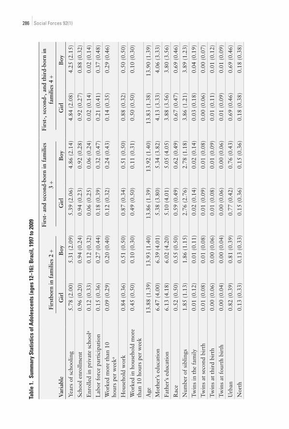
ResultsDescriptive ResultsTable 1 provides summary statistics for our analytic samples. Schooling decreases for adolescents in larger families; for example, first-, second-, and third-order girls in families of four or more children had on average almost one less year of
284 Social Forces 92(1)
schooling (0.94) than their peers in families of two or more children. We also find a gender difference favoring girls that increases in larger families—while firstborn girls in families of two or more children have 0.47 years more school-ing than boys, this difference reaches 0.59 years for adolescents in families of four or more children. Table 1 also shows that a similar proportion of firstborn adolescent boys and girls are enrolled in school in all subsamples.
The descriptive statistics for work offer a different story: they show large differences associated with both gender and birth order. For example, among firstborn adolescents in families with two or more children, 27 percent of boys but only 15 percent of girls were in the labor force. There are also large gender differences in the proportions of boys and girls performing household work. Only 51 percent of firstborn boys reported doing housework, compared to 84 percent of firstborn girls. The gender differences in housework are large in all samples.
Table 1 also shows that the mothers of the adolescents in our samples have higher levels of education than fathers; mothers’ education ranges from 4.06 to 6.47 years of schooling, depending on the sample, while fathers’ education ranges from 3.80 to 6.13. About half of the sample is non-white and, not sur-prisingly, this proportion increases among larger families. Brazil is overwhelm-ingly urban, and our samples reflect that: more than 69 percent live in urban areas, with 82 percent of firstborn adolescent girls in families of two or more children residing in urban areas.
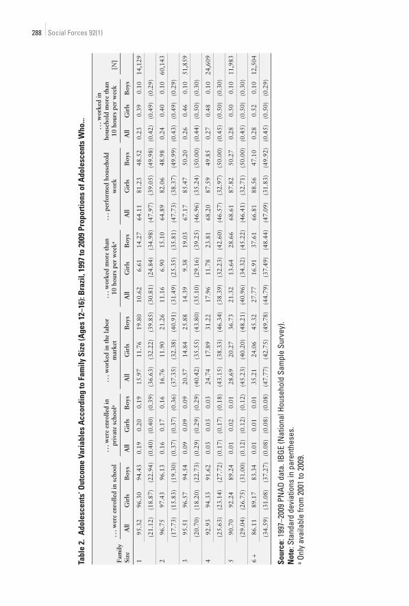
Table 2 provides the proportions of adolescents enrolled in school, enrolled in private school, participating in the labor market, and performing household work by family size. As expected, school enrollment levels are lower among ado-lescents in larger families compared to those in smaller families—95.32 percent of only-child adolescents were enrolled in school, while only 86.11 percent of their counterparts in families of six or more children were enrolled. Enrollment levels are lower among boys vis-à-vis girls, and the gap favoring girls increases in larger families. The larger the family, the smaller the proportion of adolescents enrolled in private school.
Considering the work variables, table 2 shows that the larger the family, the greater the percentage of adolescents in the labor force; only 15.97 percent of only children are in the labor force, compared to 35.21 percent of those in families of six or more children. The trend is similar for working more than ten hours a week, but the gender difference increases with family size—in families with six or more children, 37.61 percent of boys but only 16.91 percent of girls worked for more than ten hours a week. As expected, there are also gender dif-ferences in the proportions doing household work. For example, 81.23 percent of only-child girls performed household work, compared to only 48.52 percent of only-child boys. This gender difference remains in larger families. Overall, girls are overrepresented in performing household work, while boys participate in the labor force at higher rates. Notably, whereas the percentage of boys doing housework hardly varies as family size increases, the percentage of girls working in the household—which is already high—increases significantly as family size increases.
Family Size, Gender, and Birth Order in Brazil 285
Tabl
e 1.
Sum
mar
y St
atis
tics
of A
dole
scen
ts (a
ges
12–1
6): B
razi
l, 19
97 to
200
9
Var
iabl
e
Firs
tbor
n in
fam
ilies
2 +
Firs
t- a
nd s
econ
d-bo
rn in
fam
ilies
3 +
Firs
t-, s
econ
d-, a
nd t
hird
-bor
n in
fa
mili
es 4
+
Gir
lB
oyG
irl
Boy
Gir
lB
oy
Yea
rs o
f sc
hool
ing
5.78
(2.
00)
5.31
(2.
09)
5.39
(2.
06)
4.86
(2.
14)
4.84
(2.
08)
4.25
(2.
15)
Scho
ol e
nrol
lmen
t0.
96 (
0.20
)0.
94 (
0.24
)0.
94 (
0.23
)0.
92 (
0.28
)0.
92 (
0.27
)0.
88 (
0.32
)
Enr
olle
d in
pri
vate
sch
oola
0.12
(0.
33)
0.12
(0.
32)
0.06
(0.
25)
0.06
(0.
24)
0.02
(0.
14)
0.02
(0.
14)
Lab
or f
orce
par
tici
pati
on0.
15 (
0.36
)0.
27 (
0.44
)0.
18 (
0.39
)0.
32 (
0.47
)0.
21 (
0.41
)0.
37 (
0.48
)
Wor
ked
mor
e th
an 1
0 ho
urs
per
wee
ka0.
09 (
0.29
)0.
20 (
0.40
)0.
12 (
0.32
)0.
24 (
0.43
)0.
14 (
0.35
)0.
29 (
0.46
)
Hou
seho
ld w
ork
0.84
(0.
36)
0.51
(0.
50)
0.87
(0.
34)
0.51
(0.
50)
0.88
(0.
32)
0.50
(0.
50)
Wor
ked
in h
ouse
hold
mor
e th
an 1
0 ho
urs
per
wee
k0.
45 (
0.50
)0.
10 (
0.30
)0.
49 (
0.50
)0.
11 (
0.31
)0.
50 (
0.50
)0.
10 (
0.30
)
Age
13.8
8 (1
.39)
13.9
3 (1
.40)
13.8
6 (1
.39)
13.9
2 (1
.40)
13.8
3 (1
.38)
13.9
0 (1
.39)
Mot
her’
s ed
ucat
ion
6.47
(4.
00)
6.39
(4.
01)
5.38
(3.
80)
5.34
(3.
82)
4.13
(3.
33)
4.06
(3.
33)
Fath
er’s
edu
cati
on6.
13 (
4.18
)6.
02 (
4.20
)5.
10 (
4.01
)5.
05 (
4.05
)3.
88 (
3.56
)3.
80 (
3.56
)
Rac
e0.
52 (
0.50
)0.
55 (
0.50
)0.
59 (
0.49
)0.
62 (
0.49
)0.
67 (
0.47
)0.
69 (
0.46
)
Num
ber
of s
iblin
gs1.
85 (
1.13
)1.
86 (
1.15
)2.
76 (
2.76
)2.
78 (
1.18
)3.
86 (
1.21
)3.
89 (
1.23
)
Twin
s in
the
fam
ily0.
01 (
0.12
)0.
01 (
0.11
)0.
02 (
0.14
)0.
02 (
0.14
)0.
03 (
0.18
)0.
04 (
0.19
)
Twin
s at
sec
ond
birt
h0.
01 (
0.08
)0.
01 (
0.08
)0.
01 (
0.09
)0.
01 (
0.08
)0.
00 (
0.06
)0.
00 (
0.07
)
Twin
s at
thi
rd b
irth
0.00
(0.
06)
0.00
(0.
06)
0.01
(0.
08)
0.01
(0.
09)
0.01
(0.
11)
0.01
(0.
12)
Twin
s at
fou
rth
birt
h0.
00 (
0.04
)0.
00 (
0.04
)0.
00 (
0.06
)0.
00 (
0.06
)0.
01 (
0.09
)0.
01 (
0.09
)
Urb
an0.
82 (
0.39
)0.
81 (
0.39
)0.
77 (
0.42
)0.
76 (
0.43
)0.
69 (
0.46
)0.
69 (
0.46
)
Nor
th0.
13 (
0.33
)0.
13 (
0.33
)0.
15 (
0.36
)0.
15 (
0.36
)0.
18 (
0.38
)0.
18 (
0.38
)
286 Social Forces 92(1)

Multivariate ResultsTable 3 shows results for the first-stage 2SLS mod-els. The results are interesting in that they show the influence of a multiple birth on the increase in family size. The first-stage estimates are strong and suggest that a multiple birth increases family sizes by about 0.6 to 0.9. This is in line with find-ings from past research in other countries (Black, Devereux, and Salvanes 2010; Angrist, Lavy, and Schlosser 2010; Li, Zhang, and Zhu 2008). The F-statistics for the first stage are generally above 60, indicating that there are no concerns with weak instruments in the use of twins for the analyses.
Tables 4, 5, and 6 show results for the models implemented for both sexes (columns 1–3) and for females (columns 4–6) and males (columns 7–9) separately. Regression models are presented separately by subsamples. As explained above, we use different samples of adolescents corresponding to a birth order lower than that of the twins (the instrumental variable) to avoid selection problems: subsample 1 is composed of firstborn adolescents in families with at least two children; subsample 2 is composed of first- and second-borns in fami-lies with at least three children; and subsample 3 is composed of first-, second-, and third-born chil-dren in families with at least four children. The tables report coefficients for family size and coef-ficients for the dummy variables representing birth order for samples 2 and 3, which include more than one birth order.
Table 4 shows results for the models of school enrollment (panel A) and enrollment in private school (panel B). Results from logistic regression models (in columns 1, 4, and 7) and OLS regres-sion models (columns 2, 4, and 8) confirm that the higher the number of siblings, the lower the prob-ability of school enrollment. All OLS coefficients and logistic regression marginal effects representing family size in panel A are negative and statistically significant at the 0.01 level. While we do not report results for additional controls due to space limita-tions, the control variables have the expected signs. In general, rural children have worse educational outcomes than their urban peers, as do those with lower-educated parents and lower levels of family N
orth
wes
t0.
30 (
0.46
)0.
31 (
0.46
)0.
34 (
0.47
)0.
35 (
0.48
)0.
40 (
0.49
)0.
40 (
0.49
)
Sout
h0.
16 (
0.37
)0.
16 (
0.37
)0.
14 (
0.34
)0.
13 (
0.34
)0.
12 (
0.32
)0.
11 (
0.31
)
Sout
hwes
t0.
29 (
0.45
)0.
28 (
0.45
)0.
26 (
0.44
)0.
26 (
0.44
)0.
23 (
0.42
)0.
22 (
0.42
)
Cen
ter-
Wes
t0.
12 (
0.33
)0.
12 (
0.33
)0.
11 (
0.32
)0.
11 (
0.32
)0.
08 (
0.28
)0.
08 (
0.28
)
[N]
40,8
4344
,656
37,5
7140
,574
21,0
0822
,615
Sour
ce: 1
997–
2009
PN
AD d
ata.
IBGE
(Nat
iona
l Hou
seho
ld S
ampl
e Su
rvey
).N
ote:
Sta
ndar
d de
viat
ions
in p
aren
thes
es.
a Onl
y av
aila
ble
from
200
1 to
200
9.
Family Size, Gender, and Birth Order in Brazil 287
Tabl
e 2.
Ado
lesc
ents
’ Out
com
e Va
riab
les
Acc
ordi
ng to
Fam
ily S
ize
(Age
s 12
–16)
: Bra
zil,
1997
to 2
009
Prop
ortio
ns o
f Ado
lesc
ents
Who
...
Fam
ily
Size
... w
ere
enro
lled
in s
choo
l..
. wer
e en
rolle
d in
pr
ivat
e sc
hool
a..
. wor
ked
in t
he la
bor
mar
ket
... w
orke
d m
ore
than
10
hou
rs p
er w
eeka
... p
erfo
rmed
hou
seho
ld
wor
k
... w
orke
d in
ho
useh
old
mor
e th
an
10 h
ours
per
wee
k[N
]
All
Gir
lsB
oys
All
Gir
lsB
oys
All
Gir
lsB
oys
All
Gir
lsB
oys
All
Gir
lsB
oys
All
Gir
lsB
oys
195
.32
96.3
094
.43
0.19
0.20
0.19
15.9
711
.76
19.8
010
.62
6.61
14.2
764
.11
81.2
348
.52
0.23
0.39
0.10
14,1
29
(21.
12)
(18.
87)
(22.
94)
(0.4
0)(0
.40)
(0.3
9)(3
6.63
)(3
2.22
)(3
9.85
)(3
0.81
)(2
4.84
)(3
4.98
)(4
7.97
)(3
9.05
)(4
9.98
)(0
.42)
(0.4
9)(0
.29)
296
.75
97.4
396
.13
0.16
0.17
0.16
16.7
611
.90
21.2
611
.16
6.90
15.1
064
.89
82.0
648
.98
0.24
0.40
0.10
60,1
43
(17.
73)
(15.
83)
(19.
30)
(0.3
7)(0
.37)
(0.3
6)(3
7.35
)(3
2.38
)(4
0.91
)(3
1.49
)(2
5.35
)(3
5.81
)(4
7.73
)(3
8.37
)(4
9.99
)(0
.43)
(0.4
9)(0
.29)
395
.51
96.5
794
.54
0.09
0.09
0.09
20.5
714
.84
25.8
814
.39
9.38
19.0
367
.17
85.4
750
.20
0.26
0.46
0.10
51,8
59
(20.
70)
(18.
20)
(22.
73)
(0.2
9)(0
.29)
(0.2
9)(4
0.42
)(3
5.55
)(4
3.80
)(3
5.10
)(2
9.16
)(3
9.25
)(4
6.96
)(3
5.24
)(5
0.00
)(0
.44)
(0.5
0)(0
.30)
492
.93
94.3
391
.62
0.03
0.03
0.03
24.7
417
.89
31.2
217
.96
11.7
823
.81
68.2
087
.59
49.8
50.
270.
480.
1024
,609
(25.
63)
(23.
14)
(27.
72)
(0.1
7)(0
.17)
(0.1
8)(4
3.15
)(3
8.33
)(4
6.34
)(3
8.39
)(3
2.23
)(4
2.60
)(4
6.57
)(3
2.97
)(5
0.00
)(0
.45)
(0.5
0)(0
.30)
590
.70
92.2
489
.24
0.01
0.02
0.01
28.6
920
.27
36.7
321
.32
13.6
428
.66
68.6
187
.82
50.2
70.
280.
500.
1011
,983
(29.
04)
(26.
75)
(31.
00)
(0.1
2)(0
.12)
(0.1
2)(4
5.23
)(4
0.20
)(4
8.21
)(4
0.96
)(3
4.32
)(4
5.22
)(4
6.41
)(3
2.71
)(5
0.00
)(0
.45)
(0.5
0)(0
.30)
6 +
86.1
189
.17
83.3
40.
010.
010.
0135
.21
24.0
645
.32
27.7
716
.91
37.6
166
.81
88.5
647
.10
0.28
0.52
0.10
12,5
04
(34.
59)
(31.
08)
(37.
27)
(0.0
8)(0
.08)
(0.0
8)(4
7.77
)(4
2.75
)(4
9.78
)(4
4.79
)(3
7.49
)(4
8.44
)(4
7.09
)(3
1.83
)(4
9.92
)(0
.45)
(0.5
0)(0
.29)
Sour
ce: 1
997–
2009
PN
AD d
ata.
IBGE
(Nat
iona
l Hou
seho
ld S
ampl
e Su
rvey
).N
ote:
Sta
ndar
d de
viat
ions
in p
aren
thes
es.
a Onl
y av
aila
ble
from
200
1 to
200
9.
288 Social Forces 92(1)

income. Non-white adolescents are less likely to be enrolled in school than their white peers; girls have higher chances of school enrollment. Importantly, the results for the control variables are similar across all models.
The 2SLS estimates reported in column 3 reflect the effects of an additional sibling on school enrollment for adolescents who experienced an unexpected increase in family size caused by a multiple rather than a singleton birth. Contrary to the results from logistic and OLS regression models, the results from the 2SLS models show no strong adverse effects of family size on school enrollment. The coefficients are small, and only one is marginally significant (0.10 level). Analyses by gender (shown in column 6 for girls and column 9 for boys) con-firm that there is no large negative effect of family size on enrollment when we estimate models that attempt to purge the endogeneity between family size and adolescent education. However, the results in column 6 indicate that first- and second-born girls with an additional sibling have higher probabilities of school enrollment than their counterparts with one fewer sibling, though the coeffi-cients are only marginally significant at the 0.10 level. Examining the birth order coefficients, we find additional important patterns. The coefficient representing third-order adolescents is positive for girls (0.025) and statistically significant at the 0.05 level, which suggests that later-born girls have an educational advan-tage over firstborn girls, although this advantage is not related to family size.
Panel B of table 4 shows results from models similar to the ones discussed above but for private-school enrollment. Column 3 of panel B shows that an addi-
Table 3. First Stage of Two-Stage Least Squares (2SLS) Estimates of the Effect of a Twin Birth on Family Size (Ages 12–16): Brazil, 1997 to 2009
Birth Order and Gender
All Girls Boys
Coefficient [N] Coefficient [N] Coefficient [N]
Sample: First child in families of 2+ children
0.693** 85,499 0.634** 40,843 0.751** 44,656
(Instrument: twin at second order)
(0.034) (0.047) (0.048)
Sample: First and second children in families 3 +
0.852** 78,145 0.869** 37,571 0.837** 40,574
(Instrument: twin at third order)
(0.043) (0.062) (0.060)
Sample: First, second, and third children in families 4 +
0.794** 43,623 0.819** 21,008 0.775** 22,615
(Instrument: twin at fourth order)
(0.056) (0.073) (0.084)
Source: 1997–2009 PNAD data. IBGE (National Household Sample Survey).Note: Robust standard errors in parentheses.** p < 0.01
Family Size, Gender, and Birth Order in Brazil 289

Tabl
e 4.
Log
istic
(MFX
), O
rdin
ary
Leas
t Squ
are
(OLS
), an
d Tw
o-St
age
Leas
t Squ
ares
(2SL
S) E
stim
ates
of t
he E
ffect
of F
amily
Siz
e on
Ado
lesc
ents
’ Ed
ucat
iona
l Out
com
es (A
ges
12–1
6): B
razi
l, 19
97 to
200
9
Bir
th O
rder
and
Sex
All
Gir
lsB
oys
MFX
OL
S2S
LS
MFX
OL
S2S
LS
MFX
OL
S2S
LS
(1)
(2)
(3)
(4)
(5)
(6)
(7)
(8)
(9)
Pane
l A: S
choo
l Enr
ollm
ent
Sam
ple:
1st
chi
ld in
fam
ilies
of
2 +
child
ren
Fam
ily s
ize
coef
ficie
nt
(Ins
trum
ent:
tw
in a
t 2n
d)–0
.006
**–0
.018
**
0.01
3–0
.005
**–0
.016
**0.
025 +
–0.0
07**
–0.0
20**
0.00
3
(0.0
00)
(0.0
01)
(0.0
11)
(0.0
00)
(0.0
01)
(0.0
14)
(0.0
01)
(0.0
01)
(0.0
17)
[–.0
09 .0
35]
[–.0
03 .0
52]
[–.0
30 .0
36]
Sam
ple:
1st
& 2
nd c
hild
ren
in f
amili
es o
f 3
+ ch
ildre
n
Fam
ily s
ize
coef
ficie
nt–0
.008
**–0
.021
**0.
019 +
–0.0
07**
–0.0
19**
0.02
4 +
–0.0
09**
–0.0
23**
0.01
4
(Ins
trum
ent:
tw
in a
t 3r
d)(0
.000
)(0
.001
)(0
.011
)(0
.001
)(0
.001
)(0
.013
)(0
.001
)(0
.002
)(0
.017
)
Con
trol
ling
for:
[–.0
02 .0
41]
[–.0
01 .0
50]
[–.0
20 .0
47]
Seco
nd b
irth
ord
er0.
002
0.00
4*–0
.004
0.00
4*0.
007*
*0.
000
0.00
00.
000
–0.0
07
(om
itte
d: 1
st o
rder
)(0
.001
)(0
.002
)(0
.003
)(0
.002
)(0
.002
)(0
.003
)(0
.002
)(0
.003
)(0
.004
)
Sam
ple:
1st
, 2nd
, and
3rd
chi
ldre
n in
fam
ilies
of
4 +
child
ren
Fam
ily s
ize
coef
ficie
nt
(Ins
trum
ent:
tw
in a
t 4t
h)–0
.011
**–0
.019
**–0
.020
–0.0
09**
–0.0
17**
–0.0
14–0
.012
**–0
.021
**–0
.024
(0.0
01)
(0.0
01)
(0.0
20)
(0.0
01)
(0.0
02)
(0.0
27)
(0.0
01)
(0.0
02)
(0.0
30)
Con
trol
ling
for:
[–.0
60 .0
19]
[–.0
67 .0
39]
[–.0
83 .0
34]
Seco
nd b
irth
ord
er0.
004
0.00
50.
005
0.00
8*0.
011*
*0.
011 +
0.00
0–0
.001
0.00
0
(om
itte
d: 1
st o
rder
)(0
.002
)(0
.003
)(0
.005
)(0
.003
)(0
.004
)(0
.006
)(0
.004
)(0
.005
)(0
.007
)
Thi
rd b
irth
ord
er0.
016*
*0.
020*
*0.
021*
0.01
9**
0.02
6**
0.02
5*0.
012*
*0.
015*
*0.
016
(om
itte
d: 1
st o
rder
)(0
.003
)(0
.003
)(0
.009
)(0
.003
)(0
.005
)(0
.012
)(0
.004
)(0
.005
)(0
.013
)
290 Social Forces 92(1)
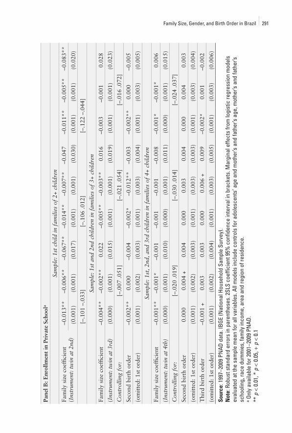
Pane
l B: E
nrol
lmen
t in
Pri
vate
Sch
oola
Sam
ple:
1st
chi
ld in
fam
ilies
of
2+ c
hild
ren
Fam
ily s
ize
coef
ficie
nt
(Ins
trum
ent:
tw
in a
t 2n
d)–0
.013
**–0
.006
**–0
.067
**–0
.014
**–0
.007
**–0
.047
–0.0
11**
–0.0
05**
–0.0
83**
(0.0
01)
(0.0
01)
(0.0
17)
(0.0
01)
(0.0
01)
(0.0
30)
(0.0
01)
(0.0
01)
(0.0
20)
[–.1
01 –
.033
][–
.106
.012
][–
.122
–.0
44]
Sam
ple:
1st
and
2nd
chi
ldre
n in
fam
ilies
of
3+ c
hild
ren
Fam
ily s
ize
coef
ficie
nt–0
.004
**–0
.002
**0.
022
–0.0
05**
–0.0
03**
0.01
6–0
.003
–0.0
010.
028
(Ins
trum
ent:
tw
in a
t 3r
d)(0
.000
)(0
.001
)(0
.015
)(0
.001
)(0
.001
)(0
.019
)(0
.001
)(0
.001
)(0
.023
)
Con
trol
ling
for:
[–.0
07 .0
51]
[–.0
21 .0
54]
[–.0
16 .0
72]
Seco
nd b
irth
ord
er–0
.002
**0.
000
–0.0
04–0
.002
*–0
.012
**–0
.003
–0.0
02**
0.00
0–0
.005
(om
itte
d: 1
st o
rder
)(0
.001
)(0
.002
)(0
.003
)(0
.001
)(0
.003
)(0
.004
)(0
.001
)(0
.003
)(0
.005
)
Sam
ple:
1st
, 2nd
, and
3rd
chi
ldre
n in
fam
ilies
of
4+ c
hild
ren
Fam
ily s
ize
coef
ficie
nt–0
.001
**–0
.001
*–0
.001
–0.0
01–0
.001
–0.0
08–0
.001
*–0
.001
*0.
006
(Ins
trum
ent:
tw
in a
t 4t
h)(0
.000
)(0
.001
)(0
.010
)(0
.000
)(0
.001
)(0
.011
)(0
.000
)(0
.001
)(0
.015
)
Con
trol
ling
for:
[–.0
20 .0
19]
[–.0
30 .0
14]
[–.0
24 .0
37]
Seco
nd b
irth
ord
er0.
000
0.00
4 +
0.00
40.
000
0.00
30.
004
0.00
00.
004
0.00
3
(om
itte
d: 1
st o
rder
)(0
.001
)(0
.002
)(0
.003
)(0
.001
)(0
.003
)(0
.003
)(0
.001
)(0
.003
)(0
.004
)
Thi
rd b
irth
ord
er–0
.001
+
0.00
30.
003
0.00
00.
006
+ 0.
009
–0.0
02*
0.00
1–0
.002
(om
itte
d: 1
st o
rder
)(0
.001
)(0
.002
)(0
.004
)(0
.001
)(0
.003
)(0
.005
)(0
.001
)(0
.003
)(0
.006
)
Sour
ce: 1
997–
2009
PN
AD d
ata.
IBGE
(Nat
iona
l Hou
seho
ld S
ampl
e Su
rvey
).N
ote:
Rob
ust s
tand
ard
erro
rs in
par
enth
eses
. 2SL
S co
effic
ient
95%
con
fiden
ce in
terv
al in
bra
cket
s. M
argi
nal e
ffect
s fro
m lo
gist
ic re
gres
sion
mod
els
eval
uate
d at
the
sam
ple
mea
n fo
r all
varia
bles
. All
mod
els
incl
ude
cont
rols
for a
dole
scen
ts’ a
ge a
nd m
othe
r’s a
nd fa
ther
’s ag
e, m
othe
r’s a
nd fa
ther
’s sc
hool
ing,
race
dum
mie
s, fa
mily
inco
me,
are
a an
d re
gion
of r
esid
ence
.a O
nly
avai
labl
e fo
r 200
1–20
09 P
NAD
.**
p <
0.0
1, *
p <
0.0
5, +
p <
0.1
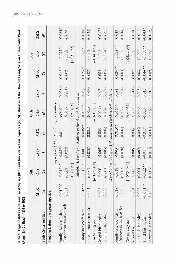
Family Size, Gender, and Birth Order in Brazil 291
Tabl
e 5.
Log
istic
(MFX
), O
rdin
ary
Leas
t Squ
are
(OLS
) and
Tw
o-St
age
Leas
t Squ
ares
(2SL
S) E
stim
ates
of t
he E
ffect
of F
amily
Siz
e on
Ado
lesc
ents
’ Wor
k (A
ges
12–1
6): B
razi
l, 19
97 to
200
9
Bir
th O
rder
and
Sex
All
Gir
lsB
oys
MFX
OL
S2S
LS
MFX
OL
S2S
LS
MFX
OL
S2S
LS
(1)
(2)
(3)
(4)
(5)
(6)
(7)
(8)
(9)
Pane
l A: L
abor
for
ce p
arti
cipa
tion
Sam
ple:
1st
chi
ld in
fam
ilies
of
2+ c
hild
ren
Fam
ily s
ize
coef
ficie
nt
(Ins
trum
ent:
tw
in a
t 2n
d)0.
015*
*0.
019*
*0.
059*
*0.
011*
*0.
016*
*0.
058 +
0.01
9**
0.02
2**
0.06
4*
(0.0
01)
(0.0
01)
(0.0
23)
`(0
.002
)(0
.034
)(0
.002
)(0
.002
)(0
.030
)
[.01
5 .1
04]
[–.0
08 .1
25]
[.00
5 .1
22]
Sam
ple:
1st
and
2nd
chi
ldre
n in
fam
ilies
of
3+ c
hild
ren
Fam
ily s
ize
coef
ficie
nt0.
015*
*0.
017*
*0.
000
0.00
8**
0.01
1**
0.03
20.
023*
*0.
023*
*–0
.030
(Ins
trum
ent:
tw
in a
t 3r
d)(0
.001
)(0
.001
)(0
.020
)(0
.002
)(0
.002
)(0
.027
)(0
.002
)(0
.002
)(0
.028
)
Con
trol
ling
for:
[–.0
39 .0
38]
[–.0
21 .0
85]
[–.0
84 .0
25]
Seco
nd b
irth
ord
er0.
003
0.00
6*0.
009*
0.00
30.
006 +
0.00
30.
004
0.00
60.
017*
(om
itte
d: 1
st o
rder
)(0
.003
)(0
.003
)(0
.005
)(0
.004
)(0
.004
)(0
.006
)(0
.005
)(0
.004
)(0
.007
)
Sam
ple:
1st
, 2nd
, and
3rd
chi
ldre
n in
fam
ilies
of
4+ c
hild
ren
Fam
ily s
ize
coef
ficie
nt
(Ins
trum
ent:
tw
in a
t 4t
h)0.
018*
*0.
018*
*0.
005
0.01
0**
0.01
1**
–0.0
320.
026*
*0.
023*
*0.
049
(0.0
02)
(0.0
02)
(0.0
28)
(0.0
02)
(0.0
02)
(0.0
34)
(0.0
03)
(0.0
03)
(0.0
46)
Con
trol
ling
for:
[–.0
50 .0
61]
[–.0
98 .0
34]
[–.0
42 .1
39]
Seco
nd b
irth
ord
er0.
004
0.00
70.
009
0.00
30.
007
0.01
4 +
0.00
70.
009
0.00
4
(om
itte
d: 1
st o
rder
)(0
.005
)(0
.005
)(0
.007
)(0
.006
)(0
.006
)(0
.008
)(0
.008
)(0
.007
)(0
.011
)
Thi
rd b
irth
ord
er–0
.031
**–0
.022
**–0
.017
–0.0
17*
–0.0
080.
010
–0.0
46**
–0.0
33**
–0.0
43*
(om
itte
d: 1
st o
rder
)(0
.006
)(0
.005
)(0
.013
)(0
.007
)(0
.007
)(0
.016
)(0
.009
)(0
.008
)(0
.019
)
292 Social Forces 92(1)
Sam
ple:
1st
chi
ld in
fam
ilies
of
2+ c
hild
ren
Fam
ily s
ize
coef
ficie
nt
(Ins
trum
ent:
tw
in a
t 2n
d)0.
011*
*0.
017*
*0.
047*
0.00
8**
0.01
3**
0.05
2 +
0.01
5**
0.02
1**
0.04
8 +
(0.0
01)
(0.0
01)
(0.0
20)
(0.0
01)
(0.0
02)
(0.0
29)
(0.0
01)
(0.0
02)
(0.0
28)
[.00
8 .0
87]
[–.0
05 .1
08]
[–.0
07 .1
03]
Sam
ple:
1st
and
2nd
chi
ldre
n in
fam
ilies
of
3+ c
hild
ren
Fam
ily s
ize
coef
ficie
nt0.
012*
*0.
016*
*0.
029
0.00
6**
0.00
8**
0.03
40.
019*
*0.
023*
*0.
024
(Ins
trum
ent:
tw
in a
t 3r
d)(0
.001
)(0
.001
)(0
.018
)(0
.001
)(0
.002
)(0
.024
)(0
.002
)(0
.002
)(0
.027
)C
ontr
ollin
g fo
r:[–
.007
.064
][–
.013
.081
][–
.029
.076
]Se
cond
bir
th o
rder
0.00
5*0.
010*
*0.
008 +
0.00
50.
009*
*0.
005
0.00
70.
012*
*0.
012 +
(om
itte
d: 1
st o
rder
)(0
.002
)(0
.003
)(0
.004
)(0
.003
)(0
.003
)(0
.005
)(0
.004
)(0
.004
)(0
.007
)Sa
mpl
e: 1
st, 2
nd, a
nd 3
rd c
hild
ren
in f
amili
es o
f 4+
chi
ldre
nFa
mily
siz
e co
effic
ient
0.01
5**
0.01
7**
–0.0
080.
008*
*0.
009*
*–0
.011
0.02
3**
0.02
2**
0.00
2(I
nstr
umen
t: t
win
at
4th)
(0.0
01)
(0.0
02)
(0.0
26)
(0.0
02)
(0.0
02)
(0.0
31)
(0.0
03)
(0.0
03)
(0.0
42)
Con
trol
ling
for:
[–.0
59 .0
44]
[–.0
71 .0
49]
[–.0
81 .0
84]
Seco
nd b
irth
ord
er0.
005
0.00
9*0.
014*
0.00
60.
011*
0.01
5*0.
005
0.01
00.
014
(om
itte
d: 1
st o
rder
)(0
.004
)(0
.004
)(0
.006
)(0
.005
)(0
.005
)(0
.007
)(0
.007
)(0
.006
)(0
.010
)T
hird
bir
th o
rder
–0.0
26**
–0.0
16**
–0.0
07–0
.010
+
0.00
00.
008
–0.0
44**
–0.0
30**
–0.0
22(o
mit
ted:
1st
ord
er)
(0.0
05)
(0.0
05)
(0.0
12)
(0.0
06)
(0.0
06)
(0.0
14)
(0.0
08)
(0.0
07)
(0.0
18)
Sour
ce: 1
997–
2009
PN
AD d
ata.
IBGE
(Nat
iona
l Hou
seho
ld S
ampl
e Su
rvey
).N
ote:
Rob
ust s
tand
ard
erro
rs in
par
enth
eses
. 2SL
S co
effic
ient
95%
con
fiden
ce in
terv
al in
bra
cket
s. M
argi
nal e
ffect
s fro
m lo
gist
ic re
gres
sion
mod
els
eval
uate
d at
the
sam
ple
mea
n fo
r all
varia
bles
. All
mod
els
incl
ude
cont
rols
for a
dole
scen
ts’ a
ge a
nd m
othe
r’s a
nd fa
ther
’s ag
e, m
othe
r’s a
nd fa
ther
’s sc
hool
ing,
race
dum
mie
s, fa
mily
inco
me,
are
a an
d re
gion
of r
esid
ence
.**
p <
0.0
1, *
p <
0.0
5, +
p <
0.1
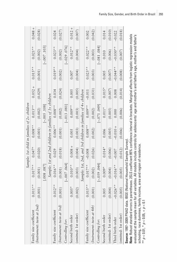
Family Size, Gender, and Birth Order in Brazil 293

Tabl
e 6.
Log
istic
(MFX
), O
rdin
ary
Leas
t Squ
are
(OLS
) and
Tw
o-St
age
Leas
t Squ
ares
(2SL
S) E
stim
ates
of t
he E
ffect
of F
amily
Siz
e on
Ado
lesc
ents
’ H
ouse
hold
Wor
k (A
ges
12–1
6): B
razi
l, 19
97 to
200
9
Bir
th O
rder
and
Sex
All
Gir
lsB
oys
MFX
OL
S2S
LS
MFX
OL
S2S
LS
MFX
OL
S2S
LS
(1)
(2)
(3)
(4)
(5)
(6)
(7)
(8)
(9)
Pane
l A: H
ouse
hold
wor
k
Sam
ple:
1st
chi
ld in
fam
ilies
of
2+ c
hild
ren
Fam
ily s
ize
coef
ficie
nt
(Ins
trum
ent:
tw
in a
t 2n
d)0.
003 +
0.00
3*0.
030
0.00
10.
000
0.00
40.
004 +
0.00
6*0.
052
(0.0
02)
(0.0
01)
(0.0
26)
(0.0
02)
(0.0
02)
(0.0
33)
(0.0
02)
(0.0
02)
(0.0
39)
[–.0
21 .0
81]
[–.0
62 .0
69]
[–.0
23 .1
28]
Sam
ple:
1st
& 2
nd c
hild
ren
in f
amili
es o
f 3+
chi
ldre
n
Fam
ily s
ize
coef
ficie
nt–0
.004
*–0
.002
0.04
5*–0
.003
–0.0
020.
020
–0.0
03–0
.001
0.06
2 +
(Ins
trum
ent:
tw
in a
t 3r
d)(0
.002
)(0
.001
)(0
.021
)(0
.002
)(0
.001
)(0
.023
)(0
.002
)(0
.002
)(0
.034
)
Con
trol
ling
for:
[.00
5 .0
86]
[–.0
25 .0
65]
[–.0
04 .1
28]
Seco
nd b
irth
ord
er–0
.011
**–0
.015
**–0
.024
**0.
005
0.00
1–0
.003
–0.0
26**
–0.0
30**
–0.0
43**
(om
itte
d: 1
st o
rder
)(0
.004
)(0
.003
)(0
.005
)(0
.003
)(0
.003
)(0
.005
)(0
.005
)(0
.005
)(0
.008
)
Sam
ple:
1st
, 2nd
, and
3rd
chi
ldre
n in
fam
ilies
of
4+ c
hild
ren
Fam
ily s
ize
coef
ficie
nt
(Ins
trum
ent:
tw
in a
t 4t
h)–0
.002
–0.0
01–0
.024
0.00
00.
001
0.01
8–0
.004
–0.0
03–0
.060
(0.0
02)
(0.0
02)
(0.0
29)
(0.0
02)
(0.0
02)
(0.0
29)
(0.0
03)
(0.0
03)
(0.0
50)
Con
trol
ling
for:
[–.0
80 .0
32]
[–.0
40 .0
75]
[–.1
58 .0
37]
Seco
nd b
irth
ord
er–0
.027
**–0
.026
**–0
.022
**–0
.006
–0.0
07–0
.009
–0.0
43**
–0.0
45**
–0.0
35**
(om
itte
d: 1
st o
rder
)(0
.005
)(0
.005
)(0
.007
)(0
.005
)(0
.005
)(0
.007
)(0
.008
)(0
.008
)(0
.012
)
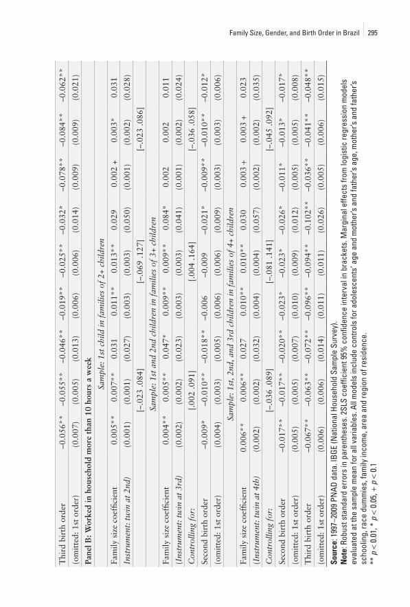
294 Social Forces 92(1)
Thi
rd b
irth
ord
er–0
.056
**–0
.055
**–0
.046
**–0
.019
**–0
.025
**–0
.032
*–0
.078
**–0
.084
**–0
.062
**
(om
itte
d: 1
st o
rder
)(0
.007
)(0
.005
)(0
.013
)(0
.006
)(0
.006
)(0
.014
)(0
.009
)(0
.009
)(0
.021
)
Pane
l B: W
orke
d in
hou
seho
ld m
ore
than
10
hour
s a
wee
k
Sam
ple:
1st
chi
ld in
fam
ilies
of
2+ c
hild
ren
Fam
ily s
ize
coef
ficie
nt
0.00
5**
0.00
7**
0.03
10.
011*
*0.
013*
*0.
029
0.00
2 +
0.00
3*0.
031
Inst
rum
ent:
tw
in a
t 2n
d)(0
.001
)(0
.001
)(0
.027
)(0
.003
)(0
.003
)(0
.050
)(0
.001
)(0
.002
)(0
.028
)
[–.0
23 .0
84]
[–.0
69 .1
27]
[–.0
23 .0
86]
Sam
ple:
1st
and
2nd
chi
ldre
n in
fam
ilies
of
3+ c
hild
ren
Fam
ily s
ize
coef
ficie
nt0.
004*
*0.
005*
*0.
047*
0.00
9**
0.00
9**
0.08
4*0.
002
0.00
20.
011
(Ins
trum
ent:
tw
in a
t 3r
d)(0
.002
)(0
.002
)(0
.023
)(0
.003
)(0
.003
)(0
.041
)(0
.001
)(0
.002
)(0
.024
)
Con
trol
ling
for:
[.00
2 .0
91]
[.00
4 .1
64]
[–.0
36 .0
58]
Seco
nd b
irth
ord
er–0
.009
*–0
.010
**–0
.018
**–0
.006
–0.0
09–0
.021
*–0
.009
**–0
.010
**–0
.012
*
(om
itte
d: 1
st o
rder
)(0
.004
)(0
.003
)(0
.005
)(0
.006
)(0
.006
)(0
.009
)(0
.003
)(0
.003
)(0
.006
)
Sam
ple:
1st
, 2nd
, and
3rd
chi
ldre
n in
fam
ilies
of
4+ c
hild
ren
Fam
ily s
ize
coef
ficie
nt0.
006*
*0.
006*
*0.
027
0.01
0**
0.01
0**
0.03
00.
003 +
0.00
3 +
0.02
3
(Ins
trum
ent:
tw
in a
t 4t
h)(0
.002
)(0
.002
)(0
.032
)(0
.004
)(0
.004
)(0
.057
)(0
.002
)(0
.002
)(0
.035
)
Con
trol
ling
for:
[–.0
36 .0
89]
[–.0
81 .1
41]
[–.0
45 .0
92]
Seco
nd b
irth
ord
er–0
.017
**–0
.017
**–0
.020
**–0
.023
*–0
.023
*–0
.026
*–0
.011
*–0
.013
*–0
.017
*
(om
itte
d: 1
st o
rder
)(0
.005
)(0
.005
)(0
.007
)(0
.010
)(0
.009
)(0
.012
)(0
.005
)(0
.005
)(0
.008
)
Thi
rd b
irth
ord
er–0
.067
**–0
.063
**–0
.072
**–0
.096
**–0
.094
**–0
.102
**–0
.036
**–0
.041
**–0
.048
**
(om
itte
d: 1
st o
rder
)(0
.006
)(0
.006
)(0
.014
)(0
.011
)(0
.011
)(0
.026
)(0
.005
)(0
.006
)(0
.015
)
Sour
ce: 1
997–
2009
PN
AD d
ata.
IBGE
(Nat
iona
l Hou
seho
ld S
ampl
e Su
rvey
).N
ote:
Rob
ust s
tand
ard
erro
rs in
par
enth
eses
. 2SL
S co
effic
ient
95%
con
fiden
ce in
terv
al in
bra
cket
s. M
argi
nal e
ffect
s fro
m lo
gist
ic re
gres
sion
mod
els
eval
uate
d at
the
sam
ple
mea
n fo
r all
varia
bles
. All
mod
els
incl
ude
cont
rols
for a
dole
scen
ts’ a
ge a
nd m
othe
r’s a
nd fa
ther
’s ag
e, m
othe
r’s a
nd fa
ther
’s sc
hool
ing,
race
dum
mie
s, fa
mily
inco
me,
are
a an
d re
gion
of r
esid
ence
.**
p <
0.0
1, *
p <
0.0
5, +
p <
0.1
Family Size, Gender, and Birth Order in Brazil 295
tional sibling is related to a 6.7-percent lower chance of private-school enroll-ment (significant at the 0.01 level). The entire 95-percent confidence interval is negative, indicating that the effect is indeed negative; however, the coefficients for the two additional subsamples are not statistically significant. The 2SLS gen-der analyses (columns 6 and 9) show that the finding of firstborn adolescents in larger families having a lower chance of private-school enrollment than their peers in smaller families reflects boys’ disadvantages (–0.083, significant at the 0.01 level).
Taken as a whole, the results for education show that most of the estimates of family size lost significance when estimated through 2SLS models.8 With one exception, our findings suggest no large adverse effects of family size on adoles-cents’ education, a result that is in line with past studies that used a twin strat-egy to estimate the causal effect of family size on education (Angrist, Lavy, and Schlosser 2010; Black, Devereux, and Salvanes 2005; Cáceres-Delpiano 2006). While it does not seem that parents invest differently in boys’ and girls’ educa-tion, boys in larger families have lower chances of private-school enrollment than their peers in smaller families, a finding that does not hold for girls.
We next examine a series of adolescents’ work outcomes. In table 5, panel A shows results for labor force participation, while panel B shows results for work-ing more than ten hours a week. All marginal effects from logistic regressions (column 1) and OLS coefficients (column 2) representing family size are positive and statistically significant at the 0.01 level, suggesting that an additional sibling is associated with higher levels of labor force participation. The 2SLS estimates are reported in column 3. The estimate for the sample of firstborn adolescents in families of two or more is positive and statistically significant at the 0.01 level (0.059), indicating that an additional sibling leads to a higher chance of working for firstborn children. The 95-percent confidence interval ranges from 0.015 to 0.104, ruling out a negative effect.
The 2SLS estimates for models stratified by gender are reported in column 6 for girls and column 9 for boys. The 2SLS estimates shown in column 6 indicate that for girls, an additional sibling does not imply a significantly higher chance of participation in the labor market: the estimate for firstborns is only mar-ginally significant, and the estimates for later-born samples are not statistically significant. The results show a different pattern for boys, with the family size coefficient (0.064) for firstborn boys significant at the 0.05 level—an additional sibling is strongly associated with pushing firstborn adolescent boys into the labor market. The lower bound of the 95-percent confidence interval approaches zero, suggesting a precisely estimated positive effect. The two additional sub-samples generate estimates that are not statistically significant. However, two coefficients representing birth order are statistically significant. The coefficient representing third-born boys in families with four or more children is –0.043 and significant at the 0.05 level, showing that third-born boys have a smaller chance of working vis-à-vis their firstborn siblings. The coefficient represent-ing second-born boys in families with three or more children is 0.017 and also significant at the 0.05 level, suggesting that second-born boys are more likely to work than firstborn boys. Because the second-order coefficient is small and
296 Social Forces 92(1)
approaches zero, these findings suggest that higher-parity boys seem to have lower chances of working than lower-parity boys. More importantly, combined, these coefficients reinforce the significance of birth order for boys’ labor market participation. The findings for working more than ten hours a week outside the home (in panel B of table 5) are very similar to the findings discussed above, though estimated with less precision.
Table 6 shows results for models of both performing any household work and working in the household for more than ten hours a week. Column 1 of panel A shows marginal effects of family size from logistic regression models, while Column 2 of panel A shows the OLS coefficients of family size. Column 3 in panel A shows estimates from the 2SLS models. When we used multiple births as an exogenous source of variation in family size, we found that an addi-tional sibling increases the probability of household work by a precisely esti-mated coefficient of 0.045 for the sample of first- and second-born adolescents. The lower bound of the 95-percent confidence interval is 0.005, suggesting that the effect is indeed positive; additional siblings increase the chances of earlier-born adolescents performing household work. Although the estimates for the additional subsamples are not statistically significant, the birth order coefficient representing second- versus first-order children is –0.024 and statistically signifi-cant at the 0.01 level, suggesting that firstborn adolescents have higher chances of performing household work than their second-born siblings, independent of family size. The coefficients representing second-order versus first-order adoles-cents (–0.022) and third-order versus first-order adolescents (–0.046) in families of four or more children confirm this birth order effect, suggesting that first-born children have higher chances of household work than their second- and third-born peers. Results of the 2SLS gender-stratified analyses are reported in columns 6 and 9. Only one coefficient representing family size is marginally sig-nificant, and not surprisingly the 95-percent confidence intervals are wider than the non-stratified analyses because of smaller sample sizes.
We next show results of models of working more than ten hours a week in the household (panel B). In comparison to the previous analysis of whether adoles-cents do any household work, these models reflect a higher level of commitment to housework, which may become increasingly incompatible with school. Both the marginal effects in columns 1, 4, and 7 of panel B and the OLS estimates in columns 2, 5, and 8 of panel B show a positive association between an addi-tional sibling and the probability of working more than ten hours a week in the household, although the estimates are very small. Column 3 of panel B shows estimates from the 2SLS models that suggest a higher probability of perform-ing more than ten hours of domestic tasks a week due to an additional sibling. The coefficient was precisely estimated for the sample of first- and second-born adolescents with two or more siblings (0.047). The estimates for the additional subsamples are not statistically significant. At the same time, both the coeffi-cient representing second- versus firstborn children in families of three or more (–0.020) and the coefficient representing second- and third-born adolescents in families of four or more (–0.072) are statistically significant at the 0.01 level;
Family Size, Gender, and Birth Order in Brazil 297

these results suggest that firstborn adolescents have a higher chance of working longer hours in the household than their later-born peers.
The 2SLS estimates of the gender-stratified analysis are reported in column 6 for girls and column 9 for boys. The family size coefficient in column 6 shows that first- and second-born girls have a higher probability of performing more than ten hours a week of domestic tasks due to an additional sibling. This coef-ficient was precisely estimated (0.084), with the lower bound of the 95-percent confidence interval at 0.004. The coefficients representing second-born (–0.026) and third-born (–0.102) are negative and statistically significant, suggesting that firstborn girls are more likely to perform more than ten hours of household tasks than their later-born counterparts.
Overall, the results suggest that—with the exception of firstborn boys enroll-ing in private school—contrary to the naïve models estimated through logistic regression and OLS, an additional sibling does not adversely affect the school participation and private-school enrollment of Brazilian adolescents. However, the findings indicate that an additional sibling is associated with a higher chance of adolescents providing resources to the family via work inside or outside the home.9 Adolescents in larger families are more likely to participate in the labor force, and this is particularly true for firstborn boys. Girls in larger families have a higher chance of performing household work, a result that is stronger for earlier-born girls.
Conclusions and DiscussionThis research uses recent nationally representative data from Brazil and a twin instrumental variable approach to examine the effects of family size on adoles-cents’ reception of resources from and provision of resources to the family. The first set of outcomes includes educational indicators—school enrollment and enrollment in private school—and reflects the influence of an additional sibling on parental investments in their children. The second set of outcomes—labor force participation and household work—reflects resources flowing from ado-lescents to the family. This paper expands previous analyses of the implications of family size for children’s welfare by considering that (1) adolescents both receive resources from and provide resources to the family; and (2) birth order and gender are key factors moderating the association between family size and these processes. To address concerns about the joint determination of children’s outcomes and family size, we use the exogenous variation produced by a twin birth to examine the effects of family size.
Our results show no strong adverse effects of family size on the educational outcomes for young cohorts of adolescents in Brazil. The findings also suggest that, in general, Brazilian families do not seem to distribute resources unequally between boys and girls and across birth orders. One exception is that firstborn boys are adversely affected in their chances of private-school enrollment—a mea-sure of the quality of the education received—by the presence of an additional sibling. To some extent, our results reinforce findings from a body of research that reported no adverse effects of family size on children’s educational outcomes
298 Social Forces 92(1)
once birth order and the endogeneity of family size and children’s outcomes were considered (Black, Devereux, and Salvanes 2005; Cáceres-Delpiano 2006).
The results for economic and household work, which focus on adolescents providing resources to the family, offer a different story. While we found a strong tendency for firstborn boys to become more likely to work outside the home with each additional sibling, the results also show that larger families are associated with a higher chance of household work for girls, particularly earlier-born girls. Although an additional sibling entails a higher tendency for girls to perform more than ten hours of household work, this is not true of boys. In this sense, our findings suggest the presence of significant gender and birth order differences in adolescents’ provision of resources to the family. Our results indi-cate that adolescents provide resources to the family in different ways and to a different extent depending on birth order and gender; an additional sibling has significantly different implications for boys vis-à-vis girls. Eradicating child and adolescent work requires comprehensive social policies that focus on multiple dimensions of their lives; our paper focuses on an important aspect of adoles-cent family life, that is, family size. Our findings underscore the importance of targeting larger families—while at the same time considering gender and birth order—for policies aimed at improving adolescent welfare through diminishing their participation in the labor force and commitment to household work.
That we found significant birth order and gender differences in the effect of family size on the provision of resources to the family but not in the reception of resources from the family confirms that family resource transfer is a dynamic process that is heavily dependent on the nature of the outcome examined. Our broad conceptualization of intra-family resource transfers has proven to be a fruitful framework for the study of the influence of family size on adolescent outcomes.
The traditional gendered allocation of work in larger families that we found in this study reflects gendered stereotypes and norms that prescribe social control and responsibilities for daughters and more independence for sons. Adolescents’ perceptions of their abilities and the differential socialization of girls and boys in their families through gendered role assignments in the provision of resources to the family place boys and girls on very different pathways that set the stage for their life course trajectories. The time spent by girls in household work and the time spent by boys in economic work produces and reinforces gender roles early in the life course of Brazilian adolescents; these gender roles have direct consequences for adolescents’ subsequent trajectories and adult lives, which should be the subject of further research and policies aimed at improving ado-lescent welfare.
Notes1. We use the terms “family size” and “number of siblings” interchangeably.2. An amendment to the 1988 Brazilian constitution established 16 as the minimum
age for work. For an excellent discussion on the meanings of child and adolescent work, see Bourdillon et al. (2010).
Family Size, Gender, and Birth Order in Brazil 299
3. Linear probability models are “computationally tractable and easily interpretable simultaneous equations model for dummy endogenous variables” (Heckman and Macurdy 1985, 28). An additional advantage of the 2SLS linear probability estima-tor is its ability to use tests of validity for over-identifying instruments and diagnostics for weak instruments (Cameron and Trivedi 2009, 471–72). This analytical approach was used in most past studies focusing on the causal effects of family size on children’s outcomes with dichotomous dependent variable and instrument (e.g., Angrist, Lavy, and Schlosser 2010; Black, Devereux, and Salvanes 2005; Càceres-Delpiano 2006; Li, Zhang, and Zhu 2008).
4. Because most studies in this area examine outcomes during adulthood (e.g., com-plete education; see Black, Devereux, and Salvanes [2005]), family income at the time these adults were growing up is impossible to measure accurately because of recollection. Because our study focuses on adolescents, our family income measure is current and does not suffer from the same recollection issues. Importantly, we calculated family income excluding adolescents’ income because it is endogenous to decisions of education and work.
5. Region and urbanicity are important determinants of employment opportunities; although we implemented models with state dummy variables, we opted to leave region and urbanicity because they consume fewer degrees of freedom and results were substantially similar.
6. To rule out concerns regarding changing variance of unobservable factors in pooled models across time, we compared the variance of the residuals in single-year models. We do not find significant changes in the variance of the residuals over time; the pooled model is preferable because it yields higher-precision estimates.
7. Robust standard errors deal with concerns about failure of estimations to meet assump-tions, such as lack of normality, autocorrelation, and heteroskedasticity. Although the coefficient estimates remain the same, the test statistics will give accurate p-values.
8. We also examined years of schooling; results also show insignificant effects of family size.
9. We tested the sensitivity of the estimates to other specifications by estimating mod-els for additional age groups and single ages. The results are qualitatively similar, but the smaller sample sizes for models estimated for single ages led to imprecise estimates.
ReferencesAngrist, J., V. Lavy, and A. Schlosser. 2010. “Multiple Experiments for the Causal Link between the Quantity
and Quality of Children.” Journal of Labor Economics 28(4):773–823.Becker, G. 1981. A Treatise on the Family. Cambridge, MA: Harvard University Press.Birdsall, N., and R. Sabot. 1996. Opportunity Foregone: Education in Brazil. Washington, DC: Inter-American
Development Bank.Black, S., P. Devereux, and K. Salvanes. 2005. “The More the Merrier? The Effect of Family Size and Birth
Order on Children’s Education.” Quarterly Journal of Economics 120(2):669–700.______. 2010. “Small Family, Smart Family? Family Size and the IQ Score of Young Men.” Journal of
Human Resources 45(1):33–58.Blake, J. 1981. Family Size and Achievement. Berkeley: University of California Press.Bourdillon, M., D. Levison, W. Myers, and B. White. 2010. Rights and Wrongs of Children’s Work. New
Brunswick, NJ: Rutgers University Press.Buchmann, C. 2000. “Family Structure, Parental Perceptions, and Child Labor in Kenya: What Factors
Determine Who Is Enrolled in School?” Social Forces 78:1349–78.
300 Social Forces 92(1)

Buchmann, C., and E. Hannum. 2001. “Education and Stratification in Developing Countries: A Review of Theories and Research.” Annual Review of Sociology 27:77–102.
Burgard, S. 2004. “Race and Pregnancy-related Care in Brazil and South Africa.” Social Science and Medicine 59:1127–46.
Cáceres-Delpiano, J. 2006. “The Impacts of Family Size on Investment in Child Quality.” Journal of Human Resources 41(4):738–54.
Cameron, A. C., and P. Trivedi. 2009. Microeconometrics Using Stata. College Station, TX: Stata Press.Carnoy, M., A. Gove, and J. Marshall. 2003. “As Razões das Diferenças de Desempenho Acadêmico na
América Latina: Dados Qualitativos do Brasil, Chile e Cuba.” Revista Brasileira de Estudos Pedagógicos 84:7–32.
Chu, C., Y. Xie, and R. Yu. 2007. “Effects of Sibship Structure Revisited: Evidence from Intrafamily Resource Transfer in Taiwan.” Sociology of Education 80:91–113.
Conley, D., and R. Glauber. 2006. “Parental Educational Investment and Children’s Academic Risk: Estimates of the Impact of Sibship Size and Birth Order from Exogenous Variation in Fertility.” Journal of Human Resources 41:722–37.
Connelly, R., D. DeGraff, and D. Levison. 1996. “Women’s Employment and Child Care in Brazil.” Economic Development and Cultural Change 44:619–56.
Dammert, A. C. 2010. “Siblings, Child Labor, and Schooling in Nicaragua and Guatemala.” Journal of Population Economics 23(1):199–224.
DeGraff, D., R. Bilsborrow, and A. Herrin. 1996. “Children’s Education in the Philippines: Does High Fertility Matter?” Population Research and Policy Review 15:219–47.
Duryea, S., D. Lam, and D. Levison. 2007. “Effect of Economic Shocks on Children’s Employment and Schooling in Brazil.” Journal of Development Economics 84(1):188–214.
Emerson, P., and A. Souza. 2008. “Birth Order, Child Labor, and School Attendance in Brazil.” World Development 36(9):1647–64.
Goldani, A. 2002. “Família, Gênero e Políticas: Famílias Brasileiras nos Anos 90 e Seus Desafios como Fator de Proteção.” Revista Brasileira de Estudos de População 19(1):29–48.
Heckman, J., and T. Macurdy. 1985. “A Simultaneous Equations Linear Probability Model.” Canadian Journal of Economics 18(1):28–37.
Hoek, J., S. Duryea, D. Lam, and D. Levison. 2009. “Dynamics of Child Labor: Labor-Force Entry and Exit in Urban Brazil.” Pp. 69–86 in Child Labor and Education in Latin America: An Economic Perspective, edited by P. Orazem, G. Sedlacek, and Z. Tzannatos. New York: Palgrave Macmillan.
Instituto Nacional de Estudos e Pesquisas Educacionais Anísio Teixeira (INEP). 2008. Resultados nacio-nais—Pisa 2006: Programa Internacional de Avaliação de Alunos (Pisa). Brasília: INEP.
Kassouf, A. 2007. “O Que Conhecemos sobre o Trabalho Infantil?” Revista Nova Economia 17(2):323–50.Kruger, D., M. Berthelon, and R. Soares. 2010. “Allocation of Children’s Time along Gender Lines: Work,
School, and Domestic Work in Brazil.” Pp. 161–92 in Child Labor and the Transition between School and Work, edited by R. Akee, E. Edmonds, and K. Tatsiramos. Bingley, UK: Emerald Group Publishing.
Lam, D., and L. Marteleto. 2006. “Small Families and Large Cohorts: The Impact of the Demographic Transition on Schooling in Brazil.” Pp. 56–83 in The Changing Transitions to Adulthood in Developing Countries: Selected Studies, edited by C. Lloyd, J. Behrman, N. Stromquist, and B. Cohen. Washington, DC: National Academies Press.
Levison, D., J. Hoek, D. Lam, and S. Duryea. 2007. “Intermittent Child Employment and Its Implications for Estimates of Child Labour.” International Labour Review 146(3–4):217–51.
Levison, D., and A. Langer. 2010. “Counting Child Domestic Servants in Latin America.” Population and Development Review 36(10):125–49.
Li, H., J. Zhang, and Y. Zhu. 2008. “The Quantity-Quality Trade-Off of Children in a Developing Country: Identification Using Chinese Twins.” Demography 45(1):223–43.
Family Size, Gender, and Birth Order in Brazil 301

Lloyd, C., and A. Blanc. 1996. “Children’s Schooling in Sub-Saharan Africa: The Role of Fathers, Mothers, and Others.” Population and Development Review 22(2):265–98.
Lloyd, C., M. Grant, and A. Ritchie. 2008. “Gender Differences in Time Use among Adolescents in Developing Countries: Implications of Rising School Enrollment Rates.” Journal of Research on Adolescence 18(1):99–120.
Lu, Y., and D. Treiman. 2008. “The Effect of Sibship Size on Educational Attainment in China: Period Variations.” American Sociological Review 73(5):813–34.
Manacorda, S., and F. Rosati. 2010. “Local Labor Demand and Child Labor.” Research in Labor Economics 31:321–54.
Marteleto, L., D. Gelber, C. Hubert, and V. Salinas. 2012. “Educational Inequalities among Latin American Adolescents: Continuities and Changes over the 1980 s, 1990 s, and 2000 s.” Research in Social Stratification and Mobility 30(3):352–75.
Mueller, E. 1984. “The Value and Allocation of Time in Rural Botswana.” Journal of Development Economics 15:329–60.
Néri, M. 2009. “O Paradoxo da Evasão e a Motivação dos Sem Escola.” Pp. 25–50 in Educação Básica no Brasil: Construindo o País do Futuro, edited by F. Veloso. Rio de Janeiro: Elsevier.
Orazem, P., P. Glewwe, and H. Patrinos. 2009. “Education.” Pp. 180–214 in Global Crises, Global Solutions: Costs and Benefits, edited by B. Lomborg. Cambridge, UK: Cambridge University Press.
Parish, W., and R. Willis. 1993. “Daughters, Education, and Family Budgets: Taiwan Experiences.” Journal of Human Resources 28:863–98.
Post, D. 2000. “Student Movements, User Fees, and Access to Mexican Higher Education: Trends in the Effect of Social Background and Family Income, 1984–1996.” Estudios Mexicanos 16:141–63.
Powell, B., R. Werum, and L. Steelman. 2004. “Linking Public Policy, Family Structure, and Educational Outcomes.” Pp. 111–44 in After the Bell: Family Background, Public Policy and Educational Success, edited by D. Conley and K. Albright. New York: Routledge.
Rosenzweig, M., and K. Wolpin. 1980. “Testing the Quantity-Quality Fertility Model: The Use of Twins as a Natural Experiment.” Econometrica 48(1):227–40.
Sastry, N., and S. Burgard. 2011. “Changes in Diarrheal Disease and Treatment among Brazilian Children from 1986 to 1996.” Population Research Policy Development 30:81–100.
Shavit, Y., and J. Pierce. 1991. “Sibship Size and Educational Attainment in Nuclear and Extended Families: Arabs and Jews in Israel.” American Sociological Review 56:321–30.
Steelman, L., and B. Powell. 1991. “Sponsoring the Next Generation: Parental Willingness to Pay for Higher Education.” American Journal of Sociology 96(6):1505–29.
Steelman, L., B. Powell, R. Werum, and S. Carter. 2002. “Reconsidering the Effects of Sibling Configuration: Recent Advances and Challenges.” Annual Review of Sociology 28:243–69.
Stromquist, N. 1997. Literacy for Citizenship: Gender and Grassroots Dynamics in Brazil. Albany: State University of New York Press.
Veloso, F. 2009. “15 Anos de Avanços na Educação no Brasil: Onde Estamos?” Pp. 3–24 in Educação Básica no Brasil: Construindo o País do Futuro, edited by F. Veloso. Rio de Janeiro: Elsevier.
Wajnman, S., and E. Rios-Neto. 1999. “Women’s Participation in the Labor Market in Brazil: Elements for Projecting Levels and Trends.” Brazilian Journal of Population Studies 2:41–54.
Wooldridge, J. 2013. Introductory Econometrics: A Modern Approach. 5th ed. Mason, OH: South-Western, Cengage Learning.
Yu, W., and K. Su. 2006. “Gender, Sibship Structure, and Educational Inequality in Taiwan: Son Preference Revisited.” Journal of Marriage and Family 68:1057–68.
Zajonc, R., and G. Markus. 1975. “Birth Order and Intellectual Development.” Psychological Review 82:74–88.
302 Social Forces 92(1)

Copyright of Social Forces is the property of Oxford University Press / USA and its contentmay not be copied or emailed to multiple sites or posted to a listserv without the copyrightholder's express written permission. However, users may print, download, or email articles forindividual use.