Embed Size (px)
Citation preview

Glasgow Theses Service http://theses.gla.ac.uk/
Graham, David Robert (2014) Extreme ultraviolet spectroscopy of impulsive phase solar flare footpoints. PhD thesis. http://theses.gla.ac.uk/5017/ Copyright and moral rights for this thesis are retained by the author A copy can be downloaded for personal non-commercial research or study, without prior permission or charge This thesis cannot be reproduced or quoted extensively from without first obtaining permission in writing from the Author The content must not be changed in any way or sold commercially in any format or medium without the formal permission of the Author When referring to this work, full bibliographic details including the author, title, awarding institution and date of the thesis must be given

Extreme Ultraviolet Spectroscopy
of Impulsive Phase Solar Flare
Footpoints
David Robert Graham, M.Sci
Astronomy and Astrophysics Group
SUPA School of Physics and Astronomy
Kelvin Building
University of Glasgow
Glasgow, G12 8QQ
Scotland, U.K.
Presented for the degree of
Doctor of Philosophy
The University of Glasgow
September 2013

This thesis is my own composition except where indicated in the text.
No part of this thesis has been submitted elsewhere for any other degree
or qualification.
Copyright c© 2013 by David R. Graham
30th September 2013

Acknowledgements
Four years suddenly does not seem like such a long time, but it certainly would have
felt far longer without the help of many fantastic people. First of all I owe a huge
thanks to my parents for getting me into this astronomy business so many years ago
with a passing trip to Jodrell Bank, and for all of the help and support over the years,
even putting up with the odd ‘project’ in the kitchen or on the driveway.
A massive thanks to my supervisor Lyndsay Fletcher for the continuous encour-
agement, inspiration, and always helping with a question or idea, especially when two
hours later it meant running back to the office to frantically scribble down another 20
ideas. Thanks also to everyone who has helped along the way, especially Iain Hannah,
Hugh Hudson, Nic Labrosse, Ryan Milligan, Helen Mason, Giulio Del Zanna, Peter
Young, David Williams, and everyone on the EIS team.
I must also thank Scott McIntosh for introducing me to the mysterious world of
spectroscopy and Genetic Algorithms, and agreeing to work with me whilst both times
expecting a baby! And of course Jørgen, Hazel, and everyone at HAO for helping me
survive in Boulder.
Thanks to everyone in the fantastic Glasgow astronomy group, past and present,
and everyone who has made a home in Room 604 (and 614!), in particular for real-
ising that 4 pm coffee and 6 pm pub are matters of religion, and of course Rachael
McLauchlan for always being able to help with so many last minute travel bookings.
I also owe many thanks to the Glasgow University Mountaineering Club, for meeting
some great friends and the countless adventures in the Scottish highlands which have
kept me (in)sane. Finally, thanks to all my friends and family for reminding me that
there is a world outside of physics, and for all the support in the form of a walk, pint,
or quick escape down the nearest singletrack.

iii
“It was precisely for that reason, to have a bit of a quieter life, that my grandfather
came and settled here — Qfwfq said — after the last supernova explosion had flung
them once more into space: grandfather, grandmother, their children, grandchildren
and great-grandchildren. The Sun was just at that stage condensing, a roundish, yel-
lowish shape, along one arm of the galaxy, and it made a good impression on him,
amidst all the other stars that were going around. ‘Let’s try a yellow one this time,’
he said to his wife.”
‘As Long as the Sun Lasts — World Memory and Other Cosmicomic Stories’ (1968)
— by Italo Calvino.

iv
for danny

Abstract
This thesis is primarily concerned with the atmospheric structure of footpoints during
the impulsive phase of a solar flare. Through spectroscopic diagnostics in Extreme-
Ultraviolet wavelengths we have made significant progress in understanding the depth
of flare heating within the atmosphere, and the energy transport processes within the
footpoint.
Chapter 1 introduces the Sun and its outer atmosphere, forming the necessary
background to understand the mechanisms behind a solar flare and their observational
characteristics. The standard flare model is presented which explains the energy source
behind a flare, through to the creation of the EUV and X-ray emission.
In Chapter 2 the basics of atomic emission line spectroscopy are introduced, covering
the processes driving electron excitation and de-excitation, the formation of Gaussian
line profiles, and the formation of density sensitive line ratios. The concept of a differ-
ential emission measure is also derived from first principles, followed by a description
of all of the instruments used throughout this thesis.
Chapter 3 presents measurements of electron density enhancements in solar flare
footpoints using diagnostics fromHinode/EIS. Using RHESSI imaging and spectroscopy,
the density enhancements are found at the location of hard X-ray footpoints and are
interpreted as the heating of layers of increasing depth in the chromosphere to coronal
temperatures.
Chapter 4 shows the first footpoint emission measure distributions (EMD) obtained
from Hinode/EIS data. A regularised inversion method was used to obtain the EMD
from emission line intensities. The gradient of the EMDs were found to be compatible

vi
with a model where the flare energy input is deposited in an upper layer of the flare
chromosphere. This top layer then cools by a conductive flux to the denser plasma
below which then radiates to balance the conductive input. The EUV footpoints are
found to be not heated directly by the injected flare energy.
In Chapter 5 electron densities of over 1013 cm−3 were found using a diagnostic at
transition region temperatures. It was shown to be difficult to heat plasma at these
depths with a thick-target flare model and several suggestions are made to explain this;
including optical depth effects, non-ionisation equilibrium, and model inaccuracies.
Finally, Chapter 6 gathered together both the density diagnostic and EMD results
to attempt to forward fit model atmospheres to observations using a Genetic Algorithm.
The results are preliminary, but progress has been made to obtain information about
the T (z) and n(z) profiles of the atmosphere via observation.

Contents
List of Figures xi
1 Introduction 1
1.1 The Sun . . . . . . . . . . . . . . . . . . . . . . . . . . . . . . . . . . . 2
1.2 The Solar Atmosphere . . . . . . . . . . . . . . . . . . . . . . . . . . . 3
1.3 Solar Flares . . . . . . . . . . . . . . . . . . . . . . . . . . . . . . . . . 8
1.3.1 Observations Characteristics . . . . . . . . . . . . . . . . . . . . 8
1.3.2 The Standard Flare Model . . . . . . . . . . . . . . . . . . . . . 11
2 Observational Diagnostics and Imaging Spectroscopy 15
2.1 Line Formation . . . . . . . . . . . . . . . . . . . . . . . . . . . . . . . 16
2.2 Density Diagnostics . . . . . . . . . . . . . . . . . . . . . . . . . . . . . 20
2.3 Differential Emission Measure in Temperature . . . . . . . . . . . . . . 24
2.4 Instrumentation . . . . . . . . . . . . . . . . . . . . . . . . . . . . . . . 28
2.4.1 Hinode EIS . . . . . . . . . . . . . . . . . . . . . . . . . . . . . 28
2.4.2 Hinode XRT . . . . . . . . . . . . . . . . . . . . . . . . . . . . . 30
2.4.3 Hinode SOT . . . . . . . . . . . . . . . . . . . . . . . . . . . . . 31
2.4.4 TRACE . . . . . . . . . . . . . . . . . . . . . . . . . . . . . . . 31
2.4.5 RHESSI . . . . . . . . . . . . . . . . . . . . . . . . . . . . . . . 32
2.4.6 IRIS . . . . . . . . . . . . . . . . . . . . . . . . . . . . . . . . . 33
3 Density and Velocity Measurements of a Solar Flare Footpoint 35
3.1 Flare Observations with Hinode EIS . . . . . . . . . . . . . . . . . . . . 36

CONTENTS viii
3.1.1 The June 5th 2007 Event . . . . . . . . . . . . . . . . . . . . . . 37
3.1.2 GOES and RHESSI . . . . . . . . . . . . . . . . . . . . . . . . . 39
3.1.3 TRACE and SOT . . . . . . . . . . . . . . . . . . . . . . . . . . 40
3.1.4 XRT . . . . . . . . . . . . . . . . . . . . . . . . . . . . . . . . . 44
3.2 Hinode EIS data . . . . . . . . . . . . . . . . . . . . . . . . . . . . . . 46
3.2.1 Data Preparation and Uncertainties . . . . . . . . . . . . . . . . 47
3.2.2 Wavelength Calibration . . . . . . . . . . . . . . . . . . . . . . 48
3.2.3 Line Analysis . . . . . . . . . . . . . . . . . . . . . . . . . . . . 51
3.3 Hinode EIS plasma diagnostics . . . . . . . . . . . . . . . . . . . . . . 54
3.3.1 Intensity, Density and Velocities across the region . . . . . . . . 55
3.3.2 Footpoint Selection . . . . . . . . . . . . . . . . . . . . . . . . . 61
3.3.3 High Velocity Flows . . . . . . . . . . . . . . . . . . . . . . . . 61
3.4 Time Evolution of Selected Footpoints . . . . . . . . . . . . . . . . . . 69
3.5 RHESSI data analysis . . . . . . . . . . . . . . . . . . . . . . . . . . . 73
3.6 Processes taking place at the flare footpoints . . . . . . . . . . . . . . . 81
3.6.1 Electron Stopping Depth . . . . . . . . . . . . . . . . . . . . . . 83
3.6.2 Electron Beam Power . . . . . . . . . . . . . . . . . . . . . . . . 85
3.6.3 Flow Speeds . . . . . . . . . . . . . . . . . . . . . . . . . . . . . 86
3.6.4 Electron Beam Heating . . . . . . . . . . . . . . . . . . . . . . . 87
3.6.5 Thermal Heating . . . . . . . . . . . . . . . . . . . . . . . . . . 88
3.7 Conclusions . . . . . . . . . . . . . . . . . . . . . . . . . . . . . . . . . 89
4 Impulsive Phase Flare Footpoint Emission Measure Distributions 91
4.1 Secrets of the EMD . . . . . . . . . . . . . . . . . . . . . . . . . . . . . 93
4.1.1 DEM to EMD . . . . . . . . . . . . . . . . . . . . . . . . . . . . 93
4.1.2 EMD Gradients . . . . . . . . . . . . . . . . . . . . . . . . . . . 94
4.1.3 Early Skylab Observations . . . . . . . . . . . . . . . . . . . . . 98
4.2 EIS Data Preparation . . . . . . . . . . . . . . . . . . . . . . . . . . . . 100
4.2.1 Line Selection . . . . . . . . . . . . . . . . . . . . . . . . . . . . 102
4.2.2 Line Flux . . . . . . . . . . . . . . . . . . . . . . . . . . . . . . 106
CONTENTS ix
4.2.3 Line Blending . . . . . . . . . . . . . . . . . . . . . . . . . . . . 108
4.3 Flare Observations and Footpoint Selection . . . . . . . . . . . . . . . . 110
4.4 DEM Technique . . . . . . . . . . . . . . . . . . . . . . . . . . . . . . . 113
4.4.1 DEM Inputs and Uncertainties . . . . . . . . . . . . . . . . . . 118
4.5 Flare EMDs . . . . . . . . . . . . . . . . . . . . . . . . . . . . . . . . . 120
4.5.1 Measured Footpoint EMD Profiles . . . . . . . . . . . . . . . . . 122
4.5.2 EMDs for Different Solar Plasmas . . . . . . . . . . . . . . . . . 123
4.5.3 Examination of the Assumptions Used . . . . . . . . . . . . . . 126
4.5.4 Varying the Abundance and Ionisation Equilibrium . . . . . . . 131
4.5.5 Electron Densities and Emitting Region Thickness . . . . . . . . 132
4.6 Discussion . . . . . . . . . . . . . . . . . . . . . . . . . . . . . . . . . . 135
4.7 Conclusions . . . . . . . . . . . . . . . . . . . . . . . . . . . . . . . . . 139
5 Measurements of High Densities in Flare Footpoints 141
5.1 Oxygen Diagnostics . . . . . . . . . . . . . . . . . . . . . . . . . . . . . 143
5.2 Fitting . . . . . . . . . . . . . . . . . . . . . . . . . . . . . . . . . . . . 145
5.3 Fitting Results . . . . . . . . . . . . . . . . . . . . . . . . . . . . . . . 149
5.4 Footpoint Densities . . . . . . . . . . . . . . . . . . . . . . . . . . . . . 151
5.5 Interpretation . . . . . . . . . . . . . . . . . . . . . . . . . . . . . . . . 155
5.5.1 A Collisional Thick Target Approach . . . . . . . . . . . . . . . 158
5.5.2 Testing for Ionisation Equilibrium . . . . . . . . . . . . . . . . . 161
5.5.3 Electron-Ion Equilibration Time . . . . . . . . . . . . . . . . . . 163
5.5.4 Testing for Optical Depth Effects . . . . . . . . . . . . . . . . . 165
5.6 Discussion . . . . . . . . . . . . . . . . . . . . . . . . . . . . . . . . . . 171
5.7 Conclusion . . . . . . . . . . . . . . . . . . . . . . . . . . . . . . . . . . 173
6 Determining Density and Temperature Profiles Through ξ(T ) and
ζ(n) 174
6.1 A Differential Emission Measure in Density - Defining the Problem . . 175
6.2 Finding n(T ) . . . . . . . . . . . . . . . . . . . . . . . . . . . . . . . . 178

CONTENTS x
6.3 Forward Fitting with PIKAIA - A Genetic Algorithm . . . . . . . . . . 179
6.3.1 Trial Models for n(h) and n(T ) . . . . . . . . . . . . . . . . . . 181
6.3.2 Test Event ξ(T ) and Line Intensities . . . . . . . . . . . . . . . 184
6.3.3 Density-Sensitive Emission Lines . . . . . . . . . . . . . . . . . 184
6.3.4 Contribution Functions . . . . . . . . . . . . . . . . . . . . . . . 185
6.3.5 The Integral . . . . . . . . . . . . . . . . . . . . . . . . . . . . . 187
6.3.6 Fitness and Residuals . . . . . . . . . . . . . . . . . . . . . . . . 188
6.4 First Results . . . . . . . . . . . . . . . . . . . . . . . . . . . . . . . . . 188
6.5 Multiple GA Realisations . . . . . . . . . . . . . . . . . . . . . . . . . . 191
6.6 Conclusions and Future Plans . . . . . . . . . . . . . . . . . . . . . . . 192
7 Conclusions and Future Work 194
Bibliography 203

List of Figures
1.1 Temperatures and densities in the solar atmosphere . . . . . . . . . . . 5
1.2 The chromosphere in Hα . . . . . . . . . . . . . . . . . . . . . . . . . . 6
1.3 CSHKP flare model . . . . . . . . . . . . . . . . . . . . . . . . . . . . . 12
1.4 CHIANTI radiative loss curve . . . . . . . . . . . . . . . . . . . . . . . 13
2.1 Term diagram for Fe xiv . . . . . . . . . . . . . . . . . . . . . . . . . . 23
2.2 Fe xiv 264/274A diagnostic ratio . . . . . . . . . . . . . . . . . . . . . 24
2.3 EIS detector schematic . . . . . . . . . . . . . . . . . . . . . . . . . . . 29
3.1 X-ray light curves for the 5th June 2007 flare . . . . . . . . . . . . . . . 39
3.2 TRACE 171 A for flaring region. . . . . . . . . . . . . . . . . . . . . . 42
3.3 TRACE and XRT imaging for the 5th June 2007 flare . . . . . . . . . . 43
3.4 Ca ii emission in the northern footpoint . . . . . . . . . . . . . . . . . 43
3.5 XRT Ti-Poly response and image at second 12-25 keV peak . . . . . . . 45
3.6 Intensities, velocities, and densities — Fe xii . . . . . . . . . . . . . . . 57
3.7 Intensities, velocities, and densities — Fe xiii . . . . . . . . . . . . . . 58
3.8 Intensities, velocities, and densities — Fe xiv . . . . . . . . . . . . . . 59
3.9 Density diagnostic curves for Fe xii, Fe xiii, and Fe xiv . . . . . . . . 60
3.10 Footpoint pixels . . . . . . . . . . . . . . . . . . . . . . . . . . . . . . . 62
3.11 High temperature velocity shifts at the first 12-25 keV peak . . . . . . 63
3.12 High velocity components in Fe xvi - 15:55:47 UT . . . . . . . . . . . . 64
3.13 High velocity components in Fe xvi - 16:01:05 UT . . . . . . . . . . . . 64
3.14 Double component fits using the R-B asymmetry constraint for Fe xvi 68

LIST OF FIGURES xii
3.15 Time evolution of Position 0 . . . . . . . . . . . . . . . . . . . . . . . . 70
3.16 Intensity variation of allowed transition . . . . . . . . . . . . . . . . . . 71
3.17 Time evolution of Position 1 . . . . . . . . . . . . . . . . . . . . . . . . 73
3.18 Time evolution of Position 2 . . . . . . . . . . . . . . . . . . . . . . . . 73
3.19 RHESSI Imaging and TRACE . . . . . . . . . . . . . . . . . . . . . . . 74
3.20 RHESSI HXR Spectra . . . . . . . . . . . . . . . . . . . . . . . . . . . 78
3.21 VAL-C and VAL-E stopping column depth for injected electrons . . . . 84
4.1 Line contributions varying in temperature, G(T ) . . . . . . . . . . . . . 106
4.2 Line contributions varying in density, G(n) . . . . . . . . . . . . . . . . 107
4.3 GOES light curves for EMD events . . . . . . . . . . . . . . . . . . . . 112
4.4 EIS rasters for EMD events . . . . . . . . . . . . . . . . . . . . . . . . 114
4.5 Test EMD solutions for α = 5.0 & α = 5.0 . . . . . . . . . . . . . . . . 118
4.6 Inverted footpoint EMDs from EIS data . . . . . . . . . . . . . . . . . 121
4.7 Footpoint, active region, and loop EMD comparison . . . . . . . . . . . 125
4.8 Inverted footpoint EMDs removing optically thick lines . . . . . . . . . 130
4.9 EMDs varying abundances and ionisation equilibrium . . . . . . . . . . 131
5.1 Term diagram for O v . . . . . . . . . . . . . . . . . . . . . . . . . . . 144
5.2 Spectrum of the 192A region from CHIANTI v7.1. . . . . . . . . . . . 148
5.3 Fitted spectra for the 192A complex . . . . . . . . . . . . . . . . . . . 150
5.4 EMDs for both footpoints in Event (a). . . . . . . . . . . . . . . . . . . 152
5.5 Diagnostic curves for ratios found in Table 5.2. . . . . . . . . . . . . . . 153
5.6 O v electron density maps . . . . . . . . . . . . . . . . . . . . . . . . . 154
5.7 Hydrogen density, electron density, and temperatures from the VAL-E
model . . . . . . . . . . . . . . . . . . . . . . . . . . . . . . . . . . . . 156
5.8 Allred flare model parameters for F10 input . . . . . . . . . . . . . . . 157
5.9 Heating rate per particle in the VAL-E atmosphere . . . . . . . . . . . 160
5.10 I192/I248 ratios for multiple temperatures . . . . . . . . . . . . . . . . . 162
5.11 O v 192A optical depth . . . . . . . . . . . . . . . . . . . . . . . . . . 168

LIST OF FIGURES xiii
6.1 Test model atmosphere . . . . . . . . . . . . . . . . . . . . . . . . . . . 182
6.2 G(n) functions for diagnostics lines . . . . . . . . . . . . . . . . . . . . 187
6.3 First GA forward model results . . . . . . . . . . . . . . . . . . . . . . 189
6.4 Residuals for test GA forward model . . . . . . . . . . . . . . . . . . . 190
6.5 1000 realisations of the GA fitting . . . . . . . . . . . . . . . . . . . . . 192

Chapter 1
Introduction
People often ask me “Why study the Sun?” It rises every morning, and as far as we
know it will do the same again tomorrow. On a good day I can normally think of at
least a handful of reasons why we should be more aware of our parent star. Starting
from the fact its vast output of energy has been the source of heat and light for life to
thrive on Earth, to understanding the many aspects of our modern life that are directly
influenced by solar activity, such as the communication satellites that guide our mobile
phones and Sat Navs, to the national power grids that light our homes, and now,
controversially, to the link between solar activity and the extreme winters of recent
years. Usually this is met with a nod or a slightly unconvinced acknowledgement. I
suppose this is understandable, most of us probably can’t recall the last time a solar
flare damaged their iPhone, so it is easy to take for granted something so seemingly
unchanging. So for a long time I went without meeting anyone outside of this field who
had first hand experience of solar activity affecting their day-to-day life. It seemed I
would be stuck in trying to convince people that what happens on the Sun can really
influence us here on Earth. At least this was the case up until a few weeks ago, after
talking to an ex-submariner. On telling them what I worked on they replied, “oh, solar
flares! We had charts to work out how to adjust the radio for them”. Apparently,
the very low frequency radio waves used to communicate with submarines at shallow
depths are disturbed by changes in the Earth’s ionosphere, a layer which solar flare

1.1: The Sun 2
X-rays easily ionise. Being able to predict the disturbance from solar activity that
day is obviously very important to be able to communicate with the crew. Of course,
this is one of many such examples. So whilst it may not be immediately apparent,
the Sun has a huge influence on our lives on many scales. Even if it simply means
the GPS takes a little longer to connect one day, or that the lights occasionally flicker
in the house. It is therefore crucial to understand what drives phenomena like solar
flares as we become more dependent on technology. So while we sip on our coffee and
contemplate the latest solar data in the comfort of an air conditioned office, we should
spare a thought for those worrying about the same, somewhere beneath the sea!
1.1 The Sun
If you are lucky enough to step outside on a clear autumn night, far from any street
lights, houses, and shops, you can marvel at the billions of stars that illuminate the
night sky. Their light makes a journey of thousands of light years across our galaxy
to reach us, by which time they are a glittering point in the sky. To be visible to us
across such vast distances means they must be immensely bright. The power behind
this luminosity is nuclear fusion in the dense core of a star, where hydrogen is fused
together releasing energy in the form of radiation.
The Sun is one of these billions of stars and is found at centre of our solar system.
It is a G-type main sequence star with a surface temperature of around 5800 degrees
Kelvin. Being within such close proximity, the Earth is intimately linked with the
physical processes governing the Sun. Over the course of a year parts of the Earth
receive slightly more or less radiation which gives rise to the seasons. For us, the dif-
ferences between summer and winter are stark, but the change in radiation received
is marginal. Should the Sun have been any one of the other classes of star, life would
have been very different indeed, if at all possible.
The Solar Interior — In the Sun fusion powers a radiating core with a temperature
of around 15 MK and an extremely high electron density of 1034 cm−3. In the core of a

1.2: The Solar Atmosphere 3
solar-like star the opacity is high enough that energetic photons released by fusion are
partially absorbed, keeping the plasma hot enough to maintain fusion, but low enough
to allow energy to eventually escape. The energy from fusion is transported by photons
which interact with the background ions and electrons taking approximately 100,000
years to reach the surface. However, as the temperature drops towards the exterior of
the star the opacity increases towards a peak. At this point radiation can no longer
transport energy efficiently and for the star to remain in hydrostatic equilibrium it
must transport energy by a new means. Since the energy transport rate has slowed
the temperature gradient becomes very steep, and at critical gradient, defined by the
Schwarzschild criterion, convection will take over from radiative transport. Areas with
a plasma density lower than the background will now continue to rise to the surface
much like hot air circulating in a heated room. Once at the surface the opacity drops
again and the plasma can radiate into open space and cool before beginning a journey
back towards the inner edge of the convective zone where the cycle is repeated. In
high resolution imaging the surface of the Sun looks somewhat like a pan of boiling
water. Granulation cells of around 1000 km in diameter appear bright in the centre,
surrounded by cooler (darker) material that is flowing back towards the core.
The solar convective zone is also observed to experience differential rotation, where
the equatorial regions of the Sun have a rotation period several days faster than at the
poles. The effect of this is to create a large shearing of the plasma at the boundary
between the radiative and convective zones known as the tachocline. The shearing
motion in this region is now accepted as a possible explanation for the generation of
large scale solar magnetic fields through a dynamo processes.
1.2 The Solar Atmosphere
The Photosphere — The photosphere is often described as the ‘surface’ of the Sun.
As there is no solid surface a definition is often made at the height where the optical
depth becomes less than τ = 1 for wavelengths in the green part of the optical spectrum
at 5000A (1A = 0.1 nm). The density above the outer edge of the convection zone drops

1.2: The Solar Atmosphere 4
off quickly with height, causing the rate of absorption of photons by negative hydrogen
ions to also fall. Photons emitted from this layer can therefore travel freely into space
without being reabsorbed. Since the photosphere is significantly brighter than the
atmosphere above, it is the layer that we see from Earth. The photosphere emits like
an almost perfect black body at a temperature of around 5700 K, radiating around
3.8× 1026 W of energy into space (Stix 2004) where on average around 1300 Wm−2 of
this is received at the Earth’s surface.
The most prominent observational feature of the photosphere are dark patches
known as sunspots, which are easily observed by projecting the solar disc onto a white
surface. It is now well established by observation and modelling that sunspots are the
locations of strong magnetic fields of several thousand Gauss originating from below
the photosphere. The plasma beta, β = 8πp/B2 where p is the gas pressure and B
is the magnetic field strength, is a ratio of the gas to magnetic pressure in a plasma.
Below the photosphere β > 1 and the gas pressure will dictate the motion of the
magnetic field. Here convective motions will ‘stir’ the magnetic field, and in places
a collection of magnetic flux tubes may emerge from below the surface and rise into
the solar atmosphere. Sunspots appear at the locations of this flux emergence, where
the magnetic field suppresses the conductive cycle and stops the flow of heat into the
photosphere (Chandrasekhar 1961). The result is that the surface temperature drops
which appears as a darker area on the solar disc.
The Chromosphere — When we talk of the solar atmosphere, we refer to the plasma
between the photosphere and the outer edge of the corona where the tenuous boundary
between interplanetary space lies. At the photosphere the hydrogen density is around
1017 cm−3 but in moving radially outward the density drops rapidly to 109 cm−3 at
the edge of the atmosphere. The atmospheric temperature and density as a function
of height has been modelled by Vernazza et al. (1981) and we show these parameters
from their quiet sun model (VAL-C) for reference in Figure 1.1. Due to the lower
density the solar atmosphere is much fainter than the photosphere. However, the
chromosphere can be viewed from Earth by optical instruments using filters at carefully

1.2: The Solar Atmosphere 5
Figure 1.1: Temperature, electron density, and neutral hydrogen density as
functions of height above the photosphere — plotted from parameters modelled
by Vernazza et al. (1981).
selected wavelengths that remove the bright contribution from the photosphere. The
absorption lines of Ca ii (singly ionised) H and K lines at 3968A and 3933A show
features close to the temperature minimum at around 500 km. The chromosphere can
also be viewed in emission during a total solar eclipse. During totality the disc occults
the photosphere and the chromosphere appears as a red ring around the dark disc
with narrow fiery structures seen extending into space known as spicules. The plasma
beta drops in favour of the magnetic field above the photosphere, and this allows
structures like spicules, extending out to 10,000 km, and cool material trapped in
magnetic loops (prominences) to form. The solar atmosphere above the photosphere is
very non-uniform as a result. Large scale super-granulation cells are also visible as the
chromospheric network which may be linked by dynamic processes with the corona. An
image in H-α of the chromosphere from the Dutch Open Telescope is found in Figure
1.2 showing the chromosphere above a sunspot where dark chromospheric fibrils trace
magnetic structures above the photosphere.
In Figure 1.1 we see that the temperature above the photosphere drops slightly to
a minimum around 500 km as would be expected for an atmosphere continuing to lose

1.2: The Solar Atmosphere 6
Figure 1.2: The chromosphere in H-α emission taken by the Dutch Open Tele-
scope. Image courtesy of the University of Utrecht and Rob Rutten.
energy from radiation and conduction. However, the presence of dynamic motions and
the magnetic field (Mariska 1992) increase the temperature again with height. Above
the minimum the temperature rises gradually to around 6000 K at a height of 1000-
2000 km. In the model by Gabriel (1976) radiative losses in the hydrogen Lyman-α
line causes another small temperature plateau at around 20,000 K and 2000 km. The
region between 500-2000 km (4000 - 20,000 K) commonly defines the chromosphere.
The Transition Region—A description of the transition region is often left to a mere
sentence in many texts, yet it is extremely important in balancing the energy transport
between the chromosphere and corona. The excellent book by John Mariska (Mariska
1992) defines the transition region as the plasma above the temperature plateau at
20,000 K and the lower edge of the corona at 106 K. The temperature gradient in this
region is extremely steep and in these models represents a height of only a few km.
Emission in this region is dominated by atomic lines such as C iv, O iv, and Si vi.
As with the chromosphere, imaging in these lines reveals that the transition region is
not a uniform layer and may be filled with funnels of plasma rising into the corona
and small loops linked to the chromospheric network (Peter 2001). The process that

1.2: The Solar Atmosphere 7
is heating the corona to over 1 MK must transfer its energy through the transition
region, and in reverse the chromosphere will also be heated through it by conduction
from hot corona. The same is true for any mass that leaves the chromosphere into the
solar wind, or returns back to the solar surface.
The Corona — Prior to the invention of the coronagraph, a telescope with an oc-
culting disc in the centre, the corona was only visible during total eclipses as white
diffuse structures extending out into space. The hot structures appear white in optical
wavelengths as the emission is predominantly photons from the photosphere scattered
by free electrons in the corona. Alongside optical observations the corona is also visi-
ble at infrared wavelengths. The magnetic field dominates the morphology of the low
density corona. The plasma can be described as frozen-in-field as the magnetic field
prevents plasma crossing between field lines. Magnetic fields originating from below
the photosphere trap hot plasma in loops reaching out to around 3 solar radii with
temperatures of 1-3 MK. The discovery of the true coronal temperature was an in-
teresting test for atomic spectroscopy. In the early 1900’s a green emission line was
observed at 5303A which could not be identified as being emitted from any known
element and was assumed to originate from a hypothetical element named coronium.
After some years of improved measurement and atomic theory it was later identified
in the 1930’s to originate from highly ionised iron, which could only be formed at the
extreme temperatures in the corona.
The processes that gives rise to the extremely high temperatures in the corona have
been a problem in solar physics for many years. One would expect the temperature
to fall off with increasing distance from the photosphere, however, some energy source
continues to heat the corona. Various models have be proposed, from the release of
magnetic energy stored in fields stressed by the motion of the photosphere, plasma wave
oscillations leaking from the photosphere and carried into the corona by structures like
spicules, and continuous eruptive events such as nano-flares (Walsh & Ireland 2003;
Hannah et al. 2011).

1.3: Solar Flares 8
1.3 Solar Flares
1.3.1 Observations Characteristics
One of the earliest documented observations of a solar flare was by R.C. Carrington
and R. Hodgson in the 19th century Carrington (1859). While projecting and drawing
a large group of sunspots Carrington witnessed extremely bright white spots growing
quickly over the sunspots. The Carrington flare was the first recorded example of a
white light flare and is regarded as being the largest flare since geomagnetic events
have been recorded. Flares of this nature are exceptionally rare, although numerous
flares of lower energy output may occur daily during periods of high solar activity.
The frequency of flares is closely correlated to the solar cycle, a roughly 11 year rise
and fall in the number of sunspots. As mentioned earlier these sunspots are formed
in regions of strong, complex magnetic fields and plasma in atmosphere above them
is confined and heated by the behaviour of these fields. An active region such as this
can be observed from UV up to soft X-Ray and extend high into the corona. During
solar minimum it is possible to observe almost no sunspots on the disc for days, or
even months in the case of the latest deep 2009-2010 minimum, and flares and eruptive
events will be rare. At solar maximum there can be several large sunspots on the disc
at one time, and their associated active regions will harbour enough energy to release
frequent flares.
A solar flare is a rapid, explosive release of colossal amounts of energy stored in the
solar atmosphere. Up to 1033 ergs of magnetic energy can be released in the space of a
few minutes to an hour with the cooling of superheated plasma visible for many hours
after. The flare is often accompanied by a readjustment of the coronal magnetic field
which can result in a coronal mass ejection (CME), an eruption of charged particles
into space, and emission across the entire electromagnetic spectrum from radio bursts
to γ-rays.
Generally, a flare can be characterised by a fast rise in soft X-ray (SXR) flux, the
impulsive phase, followed by a slower decay. The total SXR flux between 1-8 A is

1.3: Solar Flares 9
measured by the Geostationary Operational Environmental Satellites (GOES) and is
used as a classification for the size of a flare. The flare classes start at A for peak
fluxes above 10−8 W m−2, B for 10−7 W m−2, and follow the same pattern for C, M,
and X class flares. X-class flares are rare, with only a handful occurring in a year, but
are extremely energetic and are often followed by geomagnetic storms. The Halloween
storms of 2003 were the result of several X-class flares, triggering aurora as far south
as Florida and causing power outages in Sweden.
X-rays — The photon spectra of the SXR regime, around 1-10 keV, is primarily the
result of thermal bremsstrahlung radiation emitted by electrons undergoing Coulomb
collisions with ions (mostly ionised hydrogen) in a Maxwellian plasma distribution. In
this ‘free-free’ process, the electron is deflected by the ion, loosing a part of its kinetic
energy by emitting an X-ray photon. The bulk of the flare X-ray emission is emitted by
this thermal process. It is mostly emitted by hot plasma which rises and expands into
hot flare loops in the corona, but can sometimes be found in compact areas during the
impulsive phase of the flare (Mrozek & Tomczak 2004). Also important in flare spectra
are the high energy bound-bound transitions emitted by ions in high ionisation states
with filled outer shells such as Fe xvii, Ne IX, and O viii. At peak flare temperatures
of 20-30 MK ionisation states as high as Fe xxv are observed. Although these are
highly energetic transitions, with photon energies greater than 5 keV, the free-free and
free-bound processes begin to contribute more to the overall emission above 10 MK.
In the hard X-ray (HXR) energy range, 10-100 keV, the photon spectra can be
characterised by a high energy power-law tail. The primary emission process here is
non-thermal bremsstrahlung, again mostly through electron-ion interactions. As with
thermal bremsstrahlung, a photon is emitted from an electron loosing energy as it is de-
flected. However, when the incoming electrons have been accelerated, and are far more
energetic than the background plasma, the resulting photon spectra deviates from the
thermal case and takes the form of a power-law. In solar flares, an observed non-thermal
tail in the HXR photon spectra is a good indication of the presence of accelerated, or
beamed, electrons. In the thin-target approximation, the target density is low, and the

1.3: Solar Flares 10
electron beam is relatively unchanged by the few collisions (suitable in the corona). In
the thick-target case, the ambient density is high such as in the chromosphere. The
kinetic energy of the rest ion is relatively unchanged by the bremsstrahlung interaction,
and only a very small fraction (∼ 10−5) of the energy from the fast electron is lost to
bremsstrahlung emission. However, in a dense plasma, collisions with other electrons
via Coulomb collisions are much more effective at sharing the kinetic energy due to
their equal mass. Most of the beam energy in a thick-target is therefore lost in heating
the ambient plasma through electron-electron collisions. During the flare impulsive
phase, HXR emission can often be observed in compact areas deep in chromosphere.
These regions are commonly found at the base of flaring loops and are known as the
flare footpoints.
Following the work by Neupert (1968) it was shown that the rate of change of the
SXR emission is often similar to the evolution in HXR emission. We can arrive at
this conceptually if we consider that the HXR emission is proportional to the power
emitted by the flaring mechanism. If we assume that the corona stores this energy,
i.e. any losses are slow compared to the rate of energy input, then the SXR emission
found in the corona should be the integral of the HXR emission in time. For flare
observations, it is sometimes convenient to estimate the HXR evolution by taking the
time derivative of the SXR emission.
Ultraviolet & Extreme-Ultraviolet — We have discussed that the HXR footpoints
could be a location of flare heating through the interaction of non-thermal electrons
with the ambient plasma. At lower photon energies, Ultraviolet (UV) and Extreme-
Ultraviolet (EUV) line emission is also often observed at similar locations to the HXR
emission. Above the photosphere the higher temperatures and relatively low densities
change the dominantly observed spectral features from approximately a black-body
with absorption lines to emission lines and continua. The formation temperature of
these lines ranges from around 10,000 K to over 10 MK. In the flare footpoints they
are enhanced significantly with respect to the background transition region and corona.
The location of the enhancements varies during the flare evolution, and in the impulsive

1.3: Solar Flares 11
phase UV emission normally associated with the chromosphere is found to be enhanced
in bright ribbons suggesting that the emission originates from low in the solar atmo-
sphere. Along these narrow ribbons, brighter compact sources in UV and EUV may
be also found which correspond to the location of the HXR footpoints. The bulk of
the rise phase emission is therefore confined to the lower solar atmosphere. As the
flare reaches its peak, EUV emission will start to be found in loops extending from the
ribbon areas into the corona. These loops brighten significantly across the flare peak
and decay slowly during the gradual phase.
Optical — For white light emission to be viewed by projection as easily as the Car-
rington event is exceptional. However, optical emission is also observed for a wide
range of lower energy flares. Even in small events for white light to be viewed against
the photospheric background requires a large amount of energy, and it is found that a
large part of the total flare emission is in optical and UV wavelengths (Woods et al.
2006). The mechanism behind white light emission is still not well understood as it
requires the flare energy deposition to penetrate to below the chromosphere. Heating
from the chromosphere and proton beams have been suggested as possible solutions
(Fletcher et al. 2011).
1.3.2 The Standard Flare Model
It is generally accepted that the energy source for a flare lies in the coronal magnetic
field. The emergence of twisted flux from below the photosphere, and motions in the
photosphere can introduce energy into coronal loops which is stored over a period of
hours or even days. The system eventually becomes energetically unstable and will
release the stored energy, either spontaneously or from a perturbation in the field. To
produce the observed heating and non-thermal electron signatures requires a mecha-
nism that can release the coronal magnetic energy and raise electrons to non-thermal
velocities. In most current flare models, magnetic reconnection is proposed as a solution
that allows the reconfiguration of the magnetic field to a lower energy state.

1.3: Solar Flares 12
Figure 1.3: Schematic of the CSHKP flare model from Tsuneta (1997).
Over the past 30 years a relatively consistent picture has emerged for the evolution
of a solar flare. The CSHKP model has been widely used as a standard model for solar
flares based on the 2D reconnection of a single loop (Carmichael 1964; Sturrock 1966;
Hirayama 1974; Kopp & Pneuman 1976). A cartoon of the model and magnetic field
layout can be seen in Figure 1.3. The rising plasmoid is a magnetic loop or structure
which is moving and stretches the field below. As the two sides of the loop are drawn
together, the field on the inside of the loop reconnects near the ‘X-point’ (or ‘X-line’ in
2.5D), resulting in a new closed loop forming inside the original loop. Magnetic energy
is released at or near the X-point region and is directed down the loop field lines into
the footpoints. The method of energy transport is still unknown but may take the
form of plasma waves or beams of accelerated electrons.
The collisional thick-target model (Brown 1971) uses a beam of accelerated electrons
injected from the corona into the chromosphere to generate bremsstrahlung emission
and plasma heating, both of which are routinely observed in HXR and EUV spectra. A
secondary effect of the plasma heating is to drive motions in the chromospheric plasma.

1.3: Solar Flares 13
If the footpoint plasma is heated beyond the peak of the radiative loss curve (Figure
1.4) then the plasma will not be able to balance the energy input and will begin to
expand, rising back into the loop. The process is known as chromospheric evaporation,
and is observed by the Doppler shift of hot EUV lines (Doschek et al. 1980) and leads
to the hot SXR emission found in flare loops. The modelling by Fisher et al. (1985)
suggests that two types of evaporation exist, gentle and explosive. If the heating
time-scale is less than the local hydrodynamic expansion time-scale (the plasma sound
speed) then the evaporation is gentle. The evaporation is considered to be explosive
when the heating time-scale is faster than the plasma can compensate for and the flow
speeds can be above the plasma sound speed. The cut-off flare input energy between
these scenarios is around 3× 10¹⁰ ergs s−1 cm−2.
CHIANTI: radiative loss rate
104 105 106 107 108 109
Temperature (K)
10−24
10−23
10−22
10−21
Rad
iativ
e en
ergy
loss
es (
ergs
cm
3 s−
1 )
Figure 1.4: The radiative loss curve calculated by CHIANTI v7.0 (Landi et al.
2012) for a density of 1011 cm−3 and coronal abundances.
In the standard flare model the electrons are assumed to be accelerated in the
X-point region and precipitate down the magnetic field lines into the chromosphere.
This combination of magnetic reconnection and the thick-target model has been the
cornerstone of flare research for decades, primarily due to its ability to explain foot-
point HXR emission, plasma heating, and chromospheric evaporation. However, there
1.3: Solar Flares 14
is still no single agreed method in which the electrons are accelerated in the corona.
Problems also exist in transporting charged electrons from the corona to the chromo-
sphere without the ‘return current’ that exists to balance the charge and current of
this beam becoming unstable and halting or significantly redistributing the energy of
the beam electrons. Also, heating deep layers of the atmosphere to create white light
emission is challenging without very high energy electron beams. Models involving the
acceleration of electrons locally in the footpoints from the transport of plasma waves
have been proposed to solve these issues (see Russell & Fletcher (2013)).

Chapter 2
Observational Diagnostics and
Imaging Spectroscopy
This thesis is primarily concerned with diagnosing the thermodynamic properties of
solar flare footpoint plasma. Fortunately for solar physicists, much of the energy lost
by the footpoints during a flare is in the form of optically-thin line radiation, which in
UV and EUV wavelengths is rich in diagnostics of temperature, density, and plasma
dynamics. The goal of this chapter is to present the reader with sufficient background
in the atomic physics leading to these diagnostics, and the necessary assumptions in
their interpretation. We begin with an overview of the formation of optically thin
emission lines.
Observationally, an emission line can be characterised by a Gaussian line profile
and is a function of wavelength. As the next section will explain, the line emission
is the result of electrons undergoing transitions between states of quantised energies,
where photons are emitted at a wavelength inversely proportional to the difference in
energy of the two states (λ0 = hc/(E2 − E1)). For a plasma in thermal equilibrium,
the random particle velocities Doppler broaden the emission, resulting in a Gaussian
line profile centred on the rest wavelength λ0. In all fields of astronomy the most
basic of techniques is to fit a Gaussian profile of three parameters, height, centroid
position, and width, to the observed profile of a spectral line. From these three values

2.1: Line Formation 16
we can find the line intensity, velocity of the plasma relative to us, the thermal width
and therefore ion temperature, and if present, estimate the component of non-thermal
particle motions. From these relatively simple measurements, astronomers have been
able to learn an enormous amount from incredibly distance sources.
2.1 Line Formation
Line emission in plasmas and the solar atmosphere is associated with the transitions of
electrons moving between energy states of an ion or neutral atom. A variety of different
physical processes can initiate these transitions and also lead to ionisation or recom-
bination, for example; collisional excitation and de-excitation, spontaneous radiative
decay, or collisional ionisation and dielectronic recombination. The characteristic time
scale of these depends on the ion density, electron density, and the respective collision
cross sections. In the case of a quiet transition region, where the rate of absorption of
background photons is low, collisions between ions and free electrons drive the majority
of upward transitions, with radiative decay being responsible for most transitions to
lower levels. We also note that while in the transition region and corona the spectra is
dominated by emission from ions, emission lines from molecules are also found in cooler
regions of the Sun. Spectral lines from fundamental vibration-rotation transitions of
CO are seen in the µm wavelength range corresponding to temperatures of ∼ 4100 K
or even as low as 3800 K. From the work by Avrett (2003) it is apparent that these
lines are formed in the temperature minimum at around 500 km above the surface.
The balance of ionisation and recombination processes is extremely important in
understanding the observed line emission. The fractional abundance — the proportion
of a plasma in each ionisation stage — depends on this balance between the rate of
electrons leaving an ion and those recombining. The brightness of an emission line
from an ion then depends on this abundance, therefore, accurate rate calculations
and careful assumptions must be made to ensure that any diagnostics are correct.
In most cases the ionisation and recombination time scales are far longer than the
collisional excitation time scales and can be treated separately. This is the assumption

2.1: Line Formation 17
of ionisation equilibrium, and the effect of relaxing the assumption in flaring situations
will be discussed throughout this thesis.
In the case of the hot, relatively low density, corona and transition region, the
atmosphere can generally be assumed to be optically thin. The photons emitted along
the line of sight will therefore travel freely through any material between the source
and observer. At lower temperatures, and higher densities, the plasma can become
optically thick, where the emitted photons may be absorbed, scattered, or re-emitted
before reaching the observer. As mentioned, in most circumstances the optically thin
assumption is valid, although later in the thesis we have discussed circumstances where
the assumption may not hold.
The final assumption we make before calculating line intensities is to assume that
the plasma is in local thermal equilibrium. Defining the exact temperature of a plasma
can be difficult when the very nature of a plasma lends itself to be influenced by
magnetic fields and ionisation processes, this is especially true in the dynamic solar
atmosphere. Yet in the regions of the atmosphere we are concerned with, the electron-
electron collision times are very short, therefore the plasma will equilibrate quickly to
temperature changes. We can then assume that the temperature can be described by
a Maxwell-Boltzmann distribution.
The emissivity in a transition from an upper level j, to lower level i, emitted by a
volume element dV can be expressed as
dεji = njAjihνji dV erg s−1, (2.1)
where Aji is the Einstein coefficient of the transition for spontaneous emission, nj,
the number density of ions in the excited state j, and νji is the emitted frequency.
In an optically thin plasma the total flux received by an observer is found by
integrating each volume element along the line of the sight, and at a distance R is
given by
Fji =1
4πR2
∫V
njAjihνji dV erg cm−2 s−1. (2.2)
2.1: Line Formation 18
Commonly in observational studies this is reduced to an integral over the line of
sight depth; where the spatial resolution of the instrument defines the minimum area
that can be observed.
The number density of ions in the excited state nj depends on a combination of
the excitation processes mentioned above and the plasma temperature and electron
density. For many calculations it is easier to express nj as a number of ratios which
can be individually determined. We then have
nj =nj
nion
nion
nel
nel
nH
nH
ne
ne, (2.3)
where nj/nion is the relative number population of ions in the excited state com-
pared to all other levels, nion/nel is the abundance of the ionisation stage, nel/nH is
the elemental abundance relative to Hydrogen, and nH/ne is the ratio of the number
density of Hydrogen to the electron density.
In this thesis we will often refer to these quantities for deriving physical parameters
from spectra, for example, in density diagnostic ratios, differential emission measures,
and finding optical depths. We obtain these from various sources. The elemental
abundances for different parts of the solar atmosphere continue to be measured by
many authors, for example Grevesse & Sauval (1998) and Feldman et al. (1992), and
are chosen to best suit the solar plasma in question. The number density of electrons
can be measured spectroscopically or by volume estimates, and the ionisation level in
the atmosphere can be obtained through semi-empirical modelling. Theoretical atomic
physics calculations are required for each ion to find the abundance of the ionisation
level as a function of temperature, for example the percentage of Oxygen v compared to
neutral Oxygen at log T = 5.4 is 54% from Mazzotta et al. (1998). This is also true for
the relative number population nj/nion, which must be calculated by solving a system
of equations that describe the balance of all excitations and de-excitations for every
possible transition within the ion which is also sensitive to the plasma temperature and
density.
Thanks to a large and ongoing collaborative effort, the CHIANTI atomic physics

2.1: Line Formation 19
database (Dere et al. 1997) provides the most up to date calculations and atomic data
that are essential for solar and stellar spectroscopy, for which we are eternally grateful.
Compiled from theoretical work and sources such as the National Institute of Standards
and Technology (NIST), it is available for use in the Interactive Data Language (IDL).
Results of complex calculations which require many weeks of work are therefore always
available.
Moving back to describing the line emission in terms of the plasma properties, we
can group all of the terms involving the atomic physics of the line formation into a
function of temperature and density called the line contribution function, G(T, ne),
where
G(T, ne) =nj
nion
nion
nel
nel
nH
nH
ne
Aji
ne
hνji erg cm3 s−1. (2.4)
The contribution functions for each line are calculated from theory for a range of
temperatures and densities, and are often peaked strongly in temperature — this peak
temperature is often referred to as the formation temperature of the line. The observed
line flux from Equation 2.2 can now be written as
F =1
4πR2
∫V
G(T, ne)n2e dV , (2.5)
separating the atomic physics contained in the contribution functions from infor-
mation about the emitting plasma environment. The remaining term n2edV is a com-
bination of the number of free electrons and the electron density ne within a volume
element dv, and is referred to as the emission measure. The total emission measure,
defined as
EM =
∫V
n2e dV cm−3, (2.6)
is the first step in learning about the properties of the emitting plasma; as it can be
directly recovered from the measured flux of a spectral line with a known contribution

2.2: Density Diagnostics 20
function.
A very simple temperature diagnostic can be made by studying an image obtained
in one emission line. For the majority of strong lines in the EUV range the contribution
functions are strongly peaked, and an image of the emission around the line centre will
reveal bright features emitting at the formation temperature of the line. This technique
is the basis of many narrow-band imaging instruments such as TRACE and SDO/AIA.
However, the filter bandpass often includes a number of lines at different temperatures
complicating the analysis, and as we will show later, features in the solar atmosphere
are not necessarily isothermal.
2.2 Density Diagnostics
As was shown towards the end of Section 2.1 the plasma emission measure is propor-
tional to the volume of the emitting region and the square of the electron density. As
the depth along the line of sight of a footpoint is hidden to us, the volume can not be
explicitly measured from our instruments, hence the density inferred remains an upper
or lower limit derived from estimates of the emitting region height. However, we can
amend this through the use of density sensitive line ratios using the excellent spectral
coverage available on instruments such as Hinode/EIS, allowing us to make density
measurements independently of the emitting volume and other plasma properties.
Large differences in the spontaneous decay rates of allowed transitions and those
from metastable levels lead to varying density sensitivity between emission lines of the
same ion. Allowed lines follow the rules for electric dipole transitions and have large
transition probabilities. Electrons in metastable levels on the other hand must decay
either via forbidden transitions, a magnetic dipole transition which breaks the L-S
coupling selection rules, or intercombination transitions, where the electron moves to
a state with different spin. These effects greatly reduce the probability of spontaneous
decays and the emitted flux. As the electron density rises, collisional excitation and
de-excitation rates will contribute more to the level populations and the flux ratio of
the two emitted lines becomes sensitive to electron density.

2.2: Density Diagnostics 21
Three Level Case—This is best explained through an example of a simple three level
diagnostic. A ground state, Level 1, is accompanied by two upper levels where Level 3
is metastable. At low densities collisional excitation populates both upper levels and
one can assume the two level approximation; where collisional excitations are balanced
by an almost immediate decay from the upper level, and only the ground level and
excited levels are included, i.e no intermediate levels are considered. This case where
only the ground level is significantly populated is known as the coronal approximation.
The excitation and de-excitation balance for each transition can be written as
nen1C12 = n2A21, (2.7)
and
nen1C13 = n3A31, (2.8)
where n1, n2, and n3 are the level populations, C12 and C13 the collision excitation
rate coefficients, and A21 and A31 are the decay rates. The terms on the left hand
side give the number of transitions into the excited state while the number of decays
is given on the right — corresponding to the emitted flux in that transition. The flux
ratio in this case is simply proportional to the ratio of the collision rates, i.e
F31
F21
∝ C13
C12
(2.9)
As the density increases collisional excitation rates increase for both lines, and
collisional de-excitations become the increasingly preferred method of de-exciting the
metastable level since A31 and A32 are small. Level 2 will also be de-excited by colli-
sions but the contribution from spontaneous de-excitation A21 is far larger and C21 can
be ignored. The flux F21 now rises faster than F31 for two reasons. More collisional

2.2: Density Diagnostics 22
excitation results in more transitions from Level 2 to 1, but excited electrons in Level
3 may not always spontaneously decay, and collisional de-excitations from Level 3 to 2
will quickly decay, further increasing F21 compared to F31. Eventually the collisional
de-excitation rate in both lines becomes greater than the radiative decays and the flux
ratio returns to approximately the ratio of the spontaneous decay rates A31/A21. Since
the flux ratio depends on electron density and can be calculated, measurements of the
flux in both lines can be used to directly measure the electron density. However, un-
certainties will arise in the inferred density from errors in obtaining the line flux, such
as blends and fitting errors, and where the assumptions are not suitable for the plasma
conditions.
Four Level Case — The density diagnostics used throughout this thesis (see Table
2.1) can all be described by a 4 level system which is common to many EUV diagnostics
in solar and stellar atmospheres. This arises from similarities in the ions atomic struc-
ture, leading to a pair of transitions sensitive to density, where one of the upper levels
is populated by collisional excitations from a metastable level. The Fe xiv diagnostic
is perhaps the simplest configuration here, arising from the Aluminium isoelectronic
sequence with 3 electrons in the n = 3 outer shell. In this case the flux ratio of the λ274
transition, excited from the 3s2 3p 2P1/2 ground state, to the λ264 transition, excited
from the 3s2 3p 2P3/2 metastable level, is density sensitive. A term diagram for the Fe
xiv diagnostic can be found in Figure 2.1.
Levels 2, 3, and 4 are all excited via collisions from Level 1. At low densities only
Level 1 has a significant population and spontaneous decays from Level 2 to Level 1
are rare due to A21 being very small. Of the two allowed lines, the 3 → 1 transition
is brighter than 4 → 2 by around a factor of 2; this is due to the change in angular
momentum required in exciting electrons from the Level 1 2P1/2 state to the Level 4
2P3/2 state - hence C13 � C14.
As the electron density increases, further collisional excitation boosts the population
in Level 2 as electrons can not easily decay back to Level 1 — this is seen clearly in
Figure 2.2. As there is no change in angular momentum between Levels 2 and 4, the

2.2: Density Diagnostics 23
Figure 2.1: Term diagram for Fe xiv showing the four levels involved in the
density diagnostic. Level 2 is metastable and has a very low spontaneous decay
rate to Level 1 but may be populated at high densities by collisional excitations
from Level 1. The red line shows the 264A transition which is excited from the
metastable state. The ratio of this line to the 274A transition excited from the
ground state forms the density diagnostic.
collision rate C13 ≈ C24, therefore a second route is available in populating Level 4 and
the ratio F42/F31 rises with density.
At very high densities, both the metastable level and ground state populations
become balanced by collisional excitation and de-excitation, and flux ratio looses any
density sensitivity — this is shown on the left of Figure 2.2 as the ratio levels off above
1012 cm−3 at a value of 2.9.

2.3: Differential Emission Measure in Temperature 24
Figure 2.2: Diagnostic flux ratio for the Fe xiv 264/274 diagnostic. In the
left panel the flux ratio is shown across the diagnostic density range. On the
right panel the electron population in the lower level of the transitions is shown.
The population in the metastable level 3s2 3p 2P3/2 can be seen increasing with
density as collisional excitations fill the level.
2.3 Differential Emission Measure in Temperature
Many features in the solar atmosphere contain plasma at a range of temperatures, from
large scale coronal loops to more compact footpoint sources. Even in cases where a
plasma may be described as iso-thermal, the temperature distribution is often Gaus-
sian in profile. Finding the temperature distribution is of great importance for under-
standing heating and energy transfer in the solar atmosphere. As sources at different
temperatures in close proximity are never completely isolated when viewed with cur-
rent multi-band or spectral imagers, or when viewing optically thin features along the
line of sight, we require a method of recovering the temperature distribution within an
unresolved volume. Finding the differential emission measure (DEM) in temperature is
a technique used extensively throughout solar and astrophysics, returning the temper-
ature distribution of the emitting plasma by combining narrowband filter or emission
line intensity measurements sensitive to a range of temperatures.

2.3: Differential Emission Measure in Temperature 25
Table 2.1: Density sensitive line pairs used in this thesis. The left hand wave-
length in the second column denotes the transition with a metastable lower level.
For reference the isoelectronic sequence of the ion is shown and in parenthesis the
lowest similar shell configuration. The usable density range is shown in cm−3.
Ion Wavelength (A) log Tmax(K) Electron Configuration log ne range
O v 192.904 / 248.460 5.4 Be-like 10.5 - 13.5
Mg vii 280.742 / 278.404 5.8 C-like 8.5 - 11.0
Si x 258.374 / 261.057 6.2 B-like 8.0 - 10.0
Fe xii 186.854+186.887 / 195.120 6.2 P-like (N-like) 9.0 - 11.5
Fe xii 196.640 / 195.120 6.2 P-like (N-like) 9.0 - 11.5
Fe xiii 203.797+203.828 / 202.044 6.2 Si-like (C-like) 8.5 - 10.5
Fe xiv 264.789 / 274.200 6.3 Al-Like (B-like) 9.0 - 11.0
Recovering the DEM from observation is an inverse problem by nature. The ob-
served intensity is a convolution of the filter or emission lines sensitivity to tempera-
ture, and the physical properties of the source itself. Given enough sampling across the
temperature range, it is in theory possible to gather information about the source by
inversion of the data. One of the earliest and most complete definitions of the problem
is found in Craig & Brown (1976) for the application to optically thin X-Ray spectra.
We reproduce the derivation here but modified to include the contribution function
G(n, T ) for EUV emission lines.
In the previous section we saw the flux from a given emission line could be described
in terms of the plasma density and contribution function of the line (Equation 2.1). If
we define the intensity emitted by the source for an emission line α as
Iα =
∫V
G(ne(r), T )n2e(r)d
3r (2.10)
where ne(r) is the density at position r within a source volume V .
The integral over volume can transformed into one in terms of temperature by first

2.3: Differential Emission Measure in Temperature 26
expressing the volume element d3r as a surface dS at position r, hence
d3r = dS dr. (2.11)
We then divide the emitting region into surfaces of constant temperature, dST , this
can be expressed as
d3r = dS
(dr
dT
)dT = |∇T |−1 dST dT, (2.12)
where |∇T |−1 is the inverse of the temperature gradient magnitude. The volume of
plasma contained within a range of temperatures between T and T + dT is found by
integrating over the surface ST , such that
dVi =
(∫ST
|∇T |−1dS
)i
dT (2.13)
where we have used i to denote each volume of a particular temperature within the
source. At this point it is helpful to think of a map of a mountainous area with contours
drawn at set height intervals. We have so far divided the plasma into contours of
temperature and we wish to find out how much ‘mountain’ there is at each height.
Since many separate hills may share contours of the same height, but not the same
location, we must sum over these disjoint surfaces before integrating. We therefore find
the total volume between temperatures T and dT to be
dV = φ(T )dT (2.14)
where the sum over the N disjoint surfaces is given by
φ(T ) =N∑i=1
(∫ST
|∇T |−1dS
)i
. (2.15)
If we combine the new volume element with the original expression for line intensity
(Equation 2.10), the line intensity can then be described by
Iα =N∑i=1
∫T
{∫ST
G(ne(r), T )n2e(r)|∇T |−1dS
}i
dT (2.16)

2.3: Differential Emission Measure in Temperature 27
and we can define the quantity within the sum as the differential emission measure
(DEM)
ξ(T ) =N∑i=1
(∫ST
n2e(r)|∇T |−1dS
)i
. (2.17)
The abstract looking quantity ξ(T ) arises from the change from using a volume
integral to one where the plasma is treated as regions of temperature. The DEM is
essentially the amount of emitting material at a particular temperature weighted by
the local plasma density.
In this general case the density depends on the position within the temperature
surface ST . We can simplify our expression for the intensity by first defining a mean
square density, weighted by the temperature gradient over the N surfaces.
n2o(T ) =
ξ(T )
φ(T )=
∑Ni=1
(∫ST
n2e(r)|∇T |−1dS
)i∑N
i=1
(∫ST
|∇T |−1dS)i
(2.18)
In doing this we note that when the density is constant across each surface of
constant T the expression reduces to n2o(T ) = n2
e(T ), i.e the electron density of the
plasma at a temperature T . Where observations are limited by spatial resolution the
density is normally assumed to be coupled to the temperature in this manner.
Finally, if we then use the earlier expression for dV (Equation 2.14) the DEM can
be rewritten as
ξ(T ) = n2e
dV
dT(2.19)
for the case of constant surfaces of density, where n2o = n2
e, and the contribution
function can be brought outside the surface integral to give the commonly used form
of Equation 2.16,
Iα =
∫T
G(ne, T )ξ(T )dT. (2.20)
We now have an expression for the intensity emitted by a single spectral line from
within a plasma of temperature profile ξ(T ). The atomic physics G(ne, T ) is known

2.4: Instrumentation 28
for the emission line to within some uncertainty, and the density ne can be assumed
to be constant in T , however, ξ(T ) is convolved with the contribution function and
can not be immediately recovered from a single filter or emission line intensity. As
the temperature range where G(T ) is significant is small in comparison to the range
of ξ(T ) we are interested in, we can make multiple measurements of Iα for many lines
and invert the resulting matrix equation to find solutions for ξ(T ). The inversion of
Equation 2.20 is made non-trivial by uncertainties in the intensity and contribution
functions. The problem is therefore ill-posed since errors are amplified in the solution.
Techniques to minimise these problems and invert ξ(T ) are discussed later in Section
4.4.
2.4 Instrumentation
As the Earth’s atmosphere is opaque to almost all radiation with the exception of
visible light and radio, the high energy Ultraviolet and X-ray photons emitted by
energetic solar phenomena are invisible to ground based instruments. It was only with
the advent of space exploration and instruments flown on test rockets after the Second
World War that the solar spectrum could be viewed in full. The primary goal of this
thesis is to gather information about footpoint plasmas using various diagnostics in the
EUV wavelength range. These diagnostics require an instrument capable of resolving
the profile of multiple EUV emission lines, of thermal widths less than 0.5A, and from
sources of only a few arc seconds across (1′′ ∼ 725 km on the solar disc). All of the
observations used in this thesis were made used space-borne instrumentation to collect
images and spectra of solar features. We discuss the key instruments in the following.
2.4.1 Hinode EIS
Almost the entirety of the work in this thesis has been based on observations from the
Extreme Ultraviolet Imaging spectrometer (EIS, Culhane et al. (2007)) on board the
Hinode (Solar-B) mission (Kosugi et al. 2007). Launched in 2006, the primary scien-

2.4: Instrumentation 29
Figure 2.3: Schematic of the EIS light path — reproduced from Culhane et al.
(2007). Important parts to note are the entrance slit between the mirror and
grating, and the two CCDs for both short wavelength (SW) and long wavelength
(LW) emission lines.
tific objectives of Hinode were to study the transfer of energy from the photosphere
to the corona to help explain the heating of the corona, investigate the generation of
the solar magnetic field, and understand the physics behind flares and coronal mass
ejections. Hinode/EIS is currently the most advanced EUV spectrometer in flight avail-
able for flare studies and is a spiritual successor to the Coronal Diagnostic Spectrom-
eter (CDS) (Harrison et al. 1995) on the Solar and Heliospheric Observatory (SOHO)
(Domingo et al. 1995).
The EIS instrument is a normal incidence scanning slit spectrometer, operating in
the EUV with a maximum spatial resolution of 2′′ (1′′ pixel size), and 22 mA spectral
resolution (47 mA FWHM). A schematic of the spectrometer layout is shown in Figure
2.3. Light enters through a primary filter, removing any optical radiation, before being
focused by the primary mirror onto the slit. On each half of the mirror are two different
coatings, labelled L and S in the figure, and the same is found on the dispersion grating.
These two coatings allow the transmission of photons in two wavelength ranges between
170-210A and 250-290A which are dispersed by the grating onto two short and long
wavelength CCDs, (SW) and (LW).

2.4: Instrumentation 30
The 1′′ pixel size applies along the slit which has a maximum usable length of the
510′′. A 2′′ slit width can also be used or 40′′ and 266′′ slots. The rastering, or scanning,
ability of the spectrometer is achieved by a mechanism that rotates the primary mirror
along the slit axis. The slit position on the Sun can be moved in less than a second
to scan across a region, building up raster images. In each position the CCDs record
the dispersed spectrum where the y axis on the CCD is the spatial height on the Sun,
while the x axis represents the wavelength. A raster ‘image’ is therefore a data cube,
where each spatial pixel contains also the spectral information.
Exposure times in each position are normally on the order of 2-10 seconds, de-
pending on the study, and cover a small flaring region in under two minutes. The
slit positioning does not need to be contiguous and can be programmed to jump in
steps. In this case the raster is built up far quicker but at the expense of the spatial
information between the slit positions. These ‘picket-fence’ or ‘sparse’ raster modes
are sometimes desirable for flares and other quickly evolving targets.
The instrument is extremely flexible and can be programmed with a study up to
3 days in advance, where each study is designed with a specific target in mind with
exposure times, slit sizes, slit timing all adjusted to suit. The selection of pixels read
out by the CCD is important to mention here as this determines the data size of the
raster. In March 2008 Hinode developed a problem with its X-band (microwave) down-
link to Earth and has since used a backup S-band transmitter, reducing the down-link
rate from 4 Mbps to 256 Kbps. Now that the spacecraft is limited in telemetry, which
is shared with the XRT and SOT instruments (see the next two Sections), the size of
the raster and choice of spectral lines must be carefully optimised.
2.4.2 Hinode XRT
The X-Ray Telescope (XRT, Golub et al. (2007)) on board Hinode is a high spatial
and temporal resolution instrument imaging soft X-Ray emission from 6-60A. XRT em-
ploys a grazing-incidence design which focuses X-Rays onto a back-illuminated CCD
by using very shallow angles of reflection. The high photon energies of X-Rays mean

2.4: Instrumentation 31
that in traditional normal-incidence designs (such as EIS), where the mirror is ap-
proximately perpendicular to the normal of a material, they will penetrate and scatter
without significant reflection. The use of a grazing-incidence design avoids this while
still allowing continuous wavelength coverage. The large field-of-view, >30′, can im-
age entire active regions with a cadence of up to 2 seconds between exposures and by
using combinations of 9 different filters of varying material and thickness provides a
temperature response between log T = 6.0 − 7.5. In our analysis we have frequently
used it for context imaging of flaring regions, highlighting loops and brightenings at
temperatures above what EIS nominally observes.
2.4.3 Hinode SOT
For low temperature observations, Hinode has the Solar Optical Telescope (SOT,
Tsuneta et al. (2008)). SOT was arguably the most media publicised of the three
instruments, revealing spectacular high resolution movies of spicule motions in the
chromosphere. Its 50 cm telescope has a spatial resolution of 0.2′′ and images in many
broadband and narrowband filters, observing emission in the photospheric continuum
to chromospheric absorption lines. A spectro-polarimeter is also present which allows
high precision measurements of the magnetic field in the photosphere.
2.4.4 TRACE
The Transition Region And Coronal Explorer (TRACE, Handy et al. (1999)) was one
of the first NASA Small Explorer Missions (SMEX), and was launched in 1998. The
SMEX was a program that started to fund small focused missions which have often
been extremely successful; TRACE for example only stopped taking data in 2010.
TRACE imaged the photosphere, transition region, and corona with excellent spatial
and temporal resolution. Images with a pixel size of 2′′ and a 4′′ spatial resolution were
possible and could be taken every 20 seconds. Various filters covered wavelengths from
white light, UV, and EUV with responses typically less than 10A wide in the EUV. The
field of view was much smaller than its modern counterpart, the Atmospheric Imaging

2.4: Instrumentation 32
Assembly (AIA) on board the Solar Dynamics Observatory (SDO), but provided ex-
tremely high detail narrow passband images of the transition region plasma in active
regions, moss, and flare footpoints. Among the earliest discoveries with TRACE was
the detailed observation of “moss” (Fletcher & de Pontieu 1999) which can be seen as
a bright, diffuse, emission in the vicinity of coronal loops within an active region. This
hot upper transition region emission, thought to be heated plasma in the tops of small
loops, is ubiquitous in most TRACE active region images.
2.4.5 RHESSI
The Reuven Ramaty High Energy Solar Spectroscopic Imager (RHESSI) (Lin et al.
2002), launched in February 2010 was a NASA SMEX mission dedicated to the investi-
gation of energy release and deposition, and particle acceleration in solar flares. 9 cooled
germanium detectors detect X-ray photons with an energy resolution of 1-10 keV, rang-
ing from soft X-rays at 3 keV, up to 17 MeV gamma rays. This encompasses photons
emitted from the hottest flare thermal sources, around 10-30 MK, to γ-ray emission
from highly energetic processes such as the 0.511 MeV electron-positron annihilation
line.
Unlike optical and ultraviolet photons, the hard X-rays collected by RHESSI are
energetic enough to scatter in, or penetrate through, a reflective coating or grazing
incidence mirror. As a result they are difficult to focus onto a pixel based detec-
tor. Instead RHESSI makes use of a Fourier transform method to reconstruct images
(Hurford et al. 2002). Spatial information is obtained through 9 parallel grid colli-
mators placed in front of each detector. Each collimator uses a different grid pitch,
corresponding to angular resolutions ranging between 2-180′′. RHESSI rotates on its
axis every 4 seconds, which moves the grids across a bright X-ray source. The detectors
record the energy of photon, and the flux modulated by the passage of the grid over
the source. From the temporal modulations in each detector, and knowledge of the
spin timing and grid spacings, an image can be constructed from a Fourier transform
to recover the spatial information. Different combinations of detectors and grids can
2.4: Instrumentation 33
be used to optimise the reconstruction depending on the source size.
Various Fourier imaging algorithms are available but are complex and do not require
detailed discussion here. An algorithm called CLEAN is used in Chapter 3 to determine
the HXR source sizes. CLEAN was developed for radio interferometry (Hogbom 1974)
where a similar lack of spatial resolution is encountered. Through selection of the
detectors, features with a spatial size of ∼2′′ can be recovered.
The high energy resolution of the detectors allow for detailed X-ray spectroscopy.
The software package OSPEX written by R. Schwartz (Schwartz et al. 2002) contains
fitting routines suitable for thermal and non-thermal emission analysis. Corrections
are implemented to account for the absorption of photons in the collimators, scattering
in the Earth’s atmosphere, and solar background counts. OSPEX collects all of these
effects in a time dependent matrix to convert the detected photon count back to the
original source counts. Forward fitting routines are included to determine parame-
ters for models predicting bremsstrahlung emission from various electron distributions.
Models for thermal Maxwellian distributions can be fitted with parameters for the tem-
perature and total emission measure, while models of accelerated non-thermal electrons
interacting with a thin-target, or thick-target, can be fitted using forms of power laws
with a spectral index δ. OSPEX was used in Chapter 3 to determine the energy flux
in the non-thermal electrons.
2.4.6 IRIS
Though it is not used in this thesis, we briefly discuss the next solar spectroscopic
mission which can be used for flare science. The Interface Region Imaging Spectrograph
(IRIS), a NASA SMEX mission, was successfully launched on June 27th 2013. IRIS
is the next generation of imaging spectrometer, and with a spatial resolution of 0.3′′
and between 40-80mA spectral resolution will reveal features on scales never before
observed in the chromosphere. The high data rate allows for 1s cadence to quickly
raster small regions to study their temporal evolution. Flare studies with IRIS will
be of particular interest, as the spectral ranges, 1332-1358A and 1390-1406A in the

2.4: Instrumentation 34
far-UV, and 2796-2831A in the near-UV, will include many diagnostics of flare heating
in the deep chromosphere.

Chapter 3
Density and Velocity Measurements
of a Solar Flare Footpoint
This chapter begins an exploration into the atmospheric structure of impulsive phase
footpoints in solar flares using data from the Extreme-ultraviolet Imaging Spectrometer
(EIS) on board Hinode, a theme that is continued throughout this thesis. The impulsive
phase of a solar flare can be characterised by sudden increases in the hard X-ray (HXR)
light curve, the formation of compact flare footpoints in the lower atmosphere, and
strong emission in UV and EUV wavelengths. As discussed in Section 1.3, magnetic
energy stored in the corona is released by the flare mechanism, and is deposited in the
lower atmosphere during the impulsive phase, manifesting itself as plasma heating and
ionisation. The injected energy is then lost in the dense chromosphere through several
processes; by expansion of the footpoint plasma (chromospheric evaporation), radiative
losses, and conductive losses to cooler plasma. The standard interpretation of flares
suggests that most of the UV emission originates in the chromosphere while the hotter
EUV emission is found in post-flare coronal loops. However, recent work suggests that
emission in lines of highly ionised iron and calcium (Milligan & Dennis 2009), and
thermal soft X-Ray (SXR) continuum emission (Mrozek & Tomczak 2004), is clearly
seen in impulsive phase footpoints. The EIS instrument is particularly sensitive to lines
in the EUV wavelength range, and given its excellent spatial and temporal resolution,

3.1: Flare Observations with Hinode EIS 36
is well suited to such observations.
In the present chapter, we focus on measuring the electron density of the plasma
found in bright footpoints using EUV observations. The electron density is a critical
parameter in understanding the nature of heated plasmas. The solar atmosphere is
strongly stratified in temperature and density, dropping in electron density from 1013
to 109 cm−3 between the chromosphere and corona, and increasing in temperature
rapidly from 104 to 106 K. The EIS data in this chapter allows us to make diagnostics
of the electron density using line ratios for plasma temperatures which are nominally
coronal (1-3 MK). By using the diagnostics to obtain values of the electron density in
a footpoint at a specified temperature, we may be able to pinpoint the depth in the
atmosphere at which the hot emission originates. The depth will be determined by the
flare energy deposition, and knowing this is extremely important for placing limits on
the form of plasma heating in the footpoint.
3.1 Flare Observations with Hinode EIS
Line emission at these footpoint temperatures — between 50,000 MK and 10 MK —
is readily observed by the Hinode/EIS instrument. The work described in this chapter
began as an exploratory test of the diagnostic capabilities of EIS to capture, in high
spectral and spatial detail, a flare footpoint during the impulsive energy deposition
phase. More specifically, EIS rasters were selected running a “fast raster” mode that
covered the footpoint area multiple times; and which contained a range of density
sensitive line pairs (see Section 2.2 for more detail on the various modes and diagnostics
available with EIS).
The bulk of the content in this chapter was published in Graham et al. (2011).
We describe the analysis of footpoint emission from a medium sized solar flare on
5th June 2007. With coverage from Hinode/EIS fast rasters, RHESSI HXR spectra
during the impulsive phase, and EUV imaging from TRACE (see Section 2.4 for an
overview of these instruments), the range of data available made this a perfect event
to investigate the footpoint heating response. Enhanced electron densities, evaporative

3.1: Flare Observations with Hinode EIS 37
flow velocities, and the power deposited by non-thermal electrons were all estimated,
and evidence for footpoint densities increasing at a given plasma temperature during
the impulsive phase was found. RHESSI HXR spectra allowed us to show that there
was a component of non-thermal electrons in the footpoint, and from this the flare
energy input flux was estimated. We find that the enhanced densities are consistent
with a thick-target electron beam model heating progressively deeper layers of the
atmosphere. The flare energy input flux was approximately equal to the theoretical
cut-off between explosive and gentle evaporation, yet, given the uncertainties in the
HXR spectrum there is no clear case for either scenario. In the next section we present
an overview of the event as seen from multiple instruments, verifying that the enhanced
emission seen during the flare is indeed originating from the footpoints, and proceed
to explore the implications of the results.
3.1.1 The June 5th 2007 Event
To begin with, a set of EIS rasters were required that captured the impulsive phase
evolution of a footpoint and contained at least one pair of lines that were density
sensitive. Furthermore, as the field of view in most flare-specific EIS rasters is small,
we wished to view the overall morphology of the flaring region at similar wavelengths.
TRACE imaging in either the 171A or 195A filters was ideal for this purpose and was
added to the search criteria. Finally, flares with RHESSI HXR coverage were essential
if the total energy deposition in the flare was to be calculated.
A search revealed a set of raster observations using the HH AR+FLR RAS H01
study centred on NOAA active region 10960. Analysis of time variation in the EUV
emission of the active region was made using EIS data by Brooks & Warren (2009).
The authors found that the region was especially flare productive and many C and
M class flares were observed. A single C6.6 class flare which took place on June 5th
2007 was found to meet our requirements and was selected for further investigation.
The flare was observed by TRACE and RHESSI, and with several EIS rasters, during
the impulsive phase and part of the decay phase. While not part of our requirements,

3.1: Flare Observations with Hinode EIS 38
observations by the Solar Optical Telescope (SOT) and X-Ray Telescope (XRT), also
on board Hinode, proved to be very useful.
SXR light curves represent the overall evolution of a flare and we show the GOES
1-8A X-ray data for the flare in the upper panel of Figure 3.1. We see that the flare
begins at 15:50 UT, peaks at 16:13 UT, and ends at 17:00 UT. The impulsive phase is
defined as the period between the start and peak of a flare, and is relatively gradual in
this example. The benefit of this is that it was well observed by EIS, and a total of 12
EIS rasters were completed during the rise phase. TRACE and RHESSI observations
were equally well timed, although RHESSI missed the pre-flare stage and very early
evolution. Unfortunately all of instruments have missing data across the GOES peak,
which continues for around 30 minutes into the decay phase due to the nature of their
orbits.
Both Hinode and TRACE are in sun-synchronous polar orbits which are inclined
in such a way that they follow the day-night terminator above the Earth’s surface.
This allows continuous observing of the Sun for up to 9 months of the year. For the
rest of the year, the spacecraft enter an eclipse season, in which their orbits take them
behind the Earth; these eclipses account for a short fraction of the orbit not long after
launch, but as the orbit precesses this fraction can grow in time. RHESSI on the
other hand was launched into a low Earth equatorial orbit and experiences an eclipse
every orbit and it must also pass through a region of space called the South Atlantic
Anomaly (SAA, Sherrill (1991)). The Earth’s inner Van Allen radiation belt lies at a
lower altitude here, and the local energetic particle flux is much higher, thus during
passage through it RHESSI does not make observations. Unfortunately there is no way
of avoiding these occultations, which when studying transient events such as flares, can
occur with alarming synchronicity! Because of these factors, during the soft X-ray peak
of this event EIS, TRACE, and RHESSI were all obscured because of either SAA or
night-time passage and no data was taken — we have marked this on the bottom panel
of Figure 3.1. However, the majority of the impulsive phase that we are interested in
was observed, and as we will see, most of the flare energy deposition occurred during
the observed times.

3.1: Flare Observations with Hinode EIS 39
10-9
10-8
10-7
10-6
10-5
GO
ES
11
[Wm
-2]
1-8 A0.5-4 A
15:50 16:00 16:10 16:20 16:30 16:40Start Time (05-Jun-07 15:50:00)
1
10
100
RH
ES
SI C
orre
cted
Cou
nt R
ate
E R T
SAA NIGHTA1 3-6 keV6-12 keV
12-25 keV
GOES DERIV
Figure 3.1: X-ray light curves of the flare from GOES and RHESSI, top and
bottom panels respectively. The time derivative of the GOES 1−8 A channel can
be seen in red line and has been scaled to match the RHESSI light curves. The
times of the EIS rasters, TRACE images, and RHESSI images/spectra are shown
by the coloured horizontal bars at the top of the bottom panel. Also, the RHESSI
eclipse and SAA times are shown in grey with times for when the attenuating
shutters were deployed in yellow (A1) (this figure was created for Graham et al.
(2011) by I.G. Hannah).
3.1.2 GOES and RHESSI
RHESSI light curves of the X-ray count rate in 3-6 keV, 6-12 keV, and 12-25 keV
energy bands are plotted in the bottom panel of Figure 3.1. The RHESSI plots were
generated using the hessi software package for SolarSoft. Throughout this thesis any
data analysis or calculation has been performed with the Interactive Data Language
(IDL) along with the additional SolarSoft analysis package (Freeland & Handy 2012).
The counts were background subtracted and corrected for attenuating shutter positions
(see Section 3.5) by I.G. Hannah for the work in Graham et al. (2011), and are shown
in the bottom panel of Figure 3.1. Significant rises in X-ray flux above 25 keV were

3.1: Flare Observations with Hinode EIS 40
not observed in this relatively small event, which initially suggested that the non-
thermal component of the spectra would be small, however, the full spectral analysis
performed later in Section 3.5 does show evidence for a non-thermal component in
the electron spectra. Two early impulsive phase bursts are seen in the 12-25 keV light
curve (green line), occurring at 16:02 UT and 16:12 UT, which are followed by smoother
rises in the 6-12 keV (magenta), and 3-6 keV (black) curves. As discussed in Section
1.3, the time derivative of the GOES SXR flux can often be used as a proxy for the
temporal evolution of non-thermal electron deposition (Neupert 1968; Dennis & Zarro
1993). The SXR derivative, normalised to the size of the other curves, is plotted on
the bottom panel of Figure 3.1 in red, and does show two peaks coincident with the
12-25 keV emission. The fact that the harder X-ray emission is coincident with the
SXR derivative is suggestive of two distinct periods of flare heating occurring during
the event. As we do not have RHESSI observations during the GOES peak, and that
we see no third peak in the SXR derivative, we can assume that there was no additional
heating period during the data gap.
EIS rasters were available throughout the impulsive phase up to the data break
and in the decay phase. The orange coloured bars on the bottom panel of Figure 3.1
show the times of EIS rasters which were chosen to correspond with the RHESSI 12-25
keV peaks and the optimum times for RHESSI spectral analysis used later. However,
plasma velocities and densities were derived for every raster during the impulsive phase.
3.1.3 TRACE and SOT
TRACE imaging in the 171 A passband was available throughout the impulsive phase
to, coincidentally, the same point where the EIS rastering broke off. Fe ix and Fe x
contribute to most of the line emission within the 171 A passband, making it sensi-
tive to plasmas between 160,000 K and 2 MK, i.e. transition region to quiet coronal
temperatures (Handy et al. 1999; Raftery et al. 2013). TRACE images at these wave-
lengths are excellent at highlighting the overarching coronal loops (∼ 2 MK plasma) in
an active region, while cooler transition region ‘moss’ is visible as patchy background

3.1: Flare Observations with Hinode EIS 41
emission within the region (Fletcher & de Pontieu 1999). TRACE 171 A images were
prepared for this event using the standard SolarSoft trace prep software. This reads
the raw FITS files, performs a dark current and pedestal subtraction, flat field cor-
rection and replaces saturated pixels, although the images used in this chapter are for
context only and we are not concerned about any absolute intensity calibration.
We show an example image, capturing the flare at the second peak in 12-25 keV
X-rays, in Figure 3.2. The overall morphology of the region is clear in this image.
Two concentrations of magnetic field are seen at either side of the region, where bright
coronal loops fan out; these loops remain stable throughout the event. Underneath
the loops, a large patch of moss emission is seen in centre of the image. It is in this
moss area that two flare footpoint/ribbon areas are found, shown by the intense ‘U’
and inverted ‘L’ shaped ribbons. Finally, between the two footpoints, the region is
bisected by a short dark filament running diagonally from the lower-right towards the
upper-left of the image. A filament — prominence when seen in emission on the limb
— is a concentration of cool, dense, chromospheric material suspended high in the solar
atmosphere by magnetic fields. These filaments may remain stable for weeks; either
dissipating back into the atmosphere, or spontaneously erupting into the solar wind,
which we are now learning through SDO observations can be triggered by nearby flaring
activity (Kumar & Manoharan 2013). The filament in this event does not change
during the event and neither do the overlying large TRACE loops, suggesting that this
was not an eruptive flare, with no associated coronal mass ejection.
If we look at the TRACE images in sequence we see how the flare footpoints and
ribbon patterns evolve. Figure 3.3 shows a series of TRACE images which we have
cropped to the same field of view as the EIS rasters. TRACE recorded images at a
40 second cadence throughout the impulsive phase, but we have only shown the times
corresponding to the mid-point of the 5 selected EIS rasters in Figure 3.1. We have
chosen these times to best represent the evolution of the flare based on the following
considerations: (1) a frame showing the earliest signs of footpoint brightening in the
EIS rasters; (2) as the enhancements develop into more extended ribbons; (3) the
closest EIS raster corresponding to the first peak of the 12-25 keV light curve and
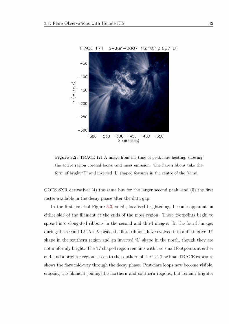
3.1: Flare Observations with Hinode EIS 42
Figure 3.2: TRACE 171 A image from the time of peak flare heating, showing
the active region coronal loops, and moss emission. The flare ribbons take the
form of bright ‘U’ and inverted ‘L’ shaped features in the centre of the frame.
GOES SXR derivative; (4) the same but for the larger second peak; and (5) the first
raster available in the decay phase after the data gap.
In the first panel of Figure 3.3, small, localised brightenings become apparent on
either side of the filament at the ends of the moss region. These footpoints begin to
spread into elongated ribbons in the second and third images. In the fourth image,
during the second 12-25 keV peak, the flare ribbons have evolved into a distinctive ‘U’
shape in the southern region and an inverted ‘L’ shape in the north, though they are
not uniformly bright. The ‘L’ shaped region remains with two small footpoints at either
end, and a brighter region is seen to the southern of the ‘U’. The final TRACE exposure
shows the flare mid-way through the decay phase. Post-flare loops now become visible,
crossing the filament joining the northern and southern regions, but remain brighter

3.1: Flare Observations with Hinode EIS 43
Figure 3.3: TRACE at 171 A images of the flaring region over several stages
during its evolution. Contours for Hinode/XRT intensities of 60% and 80% of
the maximum are shown in green and magenta. The global XRT intensity for all
images peaks around the time of the 16:10 frame, however the maximum extent
of the loop structure shown does not vary greatly.
Figure 3.4: Ca ii H emission observed by Hinode/SOT during the flare impulsive
phase taken close to the second 12-25 keV peak.
where the southern flare ribbons were located earlier. This is expected in the standard
flare model, as material evaporated from the flare footpoints (see Section 1.3.2) fills
these loops after the impulsive phase.

3.1: Flare Observations with Hinode EIS 44
We can verify that the bright areas we are referring to as footpoints and ribbons are
in fact heating in the chromosphere by inspecting the Hinode/SOT data. SOT makes
observations of the photosphere and chromosphere across a range of narrowband and
continuum filters. Narrowband images of the Ca ii H 3969.5 A line, formed around
10,000 K, were available throughout the impulsive phase, and one example is shown
in Figure 3.4. The field of view in SOT is much smaller than TRACE, however, the
upper ribbon is clear, having the same ‘L’ shape as seen in TRACE. Though the
TRACE emission at 171 A is nominally at coronal temperatures of around 1-2 MK,
here we find co-spatial intensity enhancements in a wavelength band which at non-
flaring times shows features in the chromosphere. A fundamental problem exists in
line-of-sight observations of optically thin plasmas in the solar atmosphere. As without
inferring a temperature model, or seeing a distinctive change in the structure of the
region with temperature, we can not directly measure the height of sources. In the case
above we can either interpret the ribbon as being a coronal height source with a strong
component of cooler material (10,000 K), or chromospheric material being heated to
1-2 MK. The first situation seems extremely unlikely as cool material would have to
be transported into the corona without being heated during the impulsive phase. The
second option fits conceptually with our understanding of the flare standard model.
Given the very similar shapes of the sources it is clear that in this instance it is being
emitted from chromospheric heights.
3.1.4 XRT
High temperature SXR observations, approximately coincident with the TRACE ex-
posures, were also available from Hinode/XRT using the Ti-Poly filter. The XRT
instrument uses a range of filters varying in opacity and temperature sensitivity to the
SXR emission. As with TRACE, a SolarSoft routine xrt prep was run to prepare
the data, performing dark frame and flat field subtractions, along with cosmic ray and
radiation belt noise removal. An example unsaturated XRT image taken during the
impulsive phase with the Ti-Poly filter is shown on the right of Figure 3.5. Plasma

3.1: Flare Observations with Hinode EIS 45
around 8 MK is visible in this image, assuming that most of the observed emission is
near the peak of the filter response (plotted on the left of Figure 3.5), and highlights
hot loop structures above the transition region which connect 3 more concentrated
points of bright emission.
During observations, XRT exposures are adjusted using an automatic exposure
control to avoid saturation, however, during flares the lower opacity filters can still
often saturate even for low exposure times, limiting the selection of images. With
this in mind, images that best matched the TRACE exposure times were selected
but could not always be exactly coincident. The XRT emission was plotted over the
TRACE images in Figure 3.3 using contours of 60% (green) and 80% (magenta) of the
maximum image intensity. We found that the visible edges of the loops found in Figure
3.5 were well defined by a 60% contour, while 80% highlighted the smaller bright areas,
hence using the same contours over the TRACE images.
Figure 3.5: The Ti-Poly filter temperature response is shown in the left hand
plot peaking at log T = 6.9 K. On the right is a Ti-Poly image from XRT taken
at the same time as the centre TRACE image in Figure 3.3. Hot loop structures
are visible in addition to compact enhancements near the loop footpoints and in
the centre of the moss region.

3.2: Hinode EIS data 46
In the first panel the XRT exposure was taken 105 seconds after TRACE. In panels
2-4 they are within 20 seconds of each other, and in the final panel XRT followed
TRACE by 2 minutes. In the centre 3 panels the brightest emission (80% contours)
was found to match well with the TRACE ribbon brightenings, while the 60% contours
outlined the extent of the moss regions. It was therefore straightforward to correct for
the pointing difference between TRACE and XRT by moving the XRT images by hand.
An offset of 2′′ in the x and 29′′ in the y directions was found in all exposures.
XRT emission in the first panel was saturated but defined the outer extent of the
flaring region. As the impulsive phase progressed the loops became brighter but their
overall size and shape changed little. The two bright TRACE 171 A footpoints in the
north, and the single ribbon area in the south, also became increasingly well bounded
by the brightest XRT emission (magenta contour), with the 80% intensity contour
completely surrounding the flare ribbon in the fourth image. The observation that at
least part of the hot SXR emission is contained within the same location of the TRACE
bright points is compelling, and supports our view that TRACE is indeed showing us
flare footpoints. Secondly, it demonstrates that the footpoint plasma present reaches
temperatures of up to 8 MK, but without imaging in others filters we cannot determine
this temperature with any more accuracy.
3.2 Hinode EIS data
A sequence of 12 EIS rasters using the HH AR+FLR RAS H01 study were found
running during the flare impulsive phase, with more following in the decay phase after
the data break. The study is a sparse, fast-raster mode, meaning that the spectrometer
slit scans across a small region quickly in non-contiguous steps, making multiple rasters
during the evolution of the event. These rasters scanned East to West over a region of
240′′ by 240′′ by moving the 1′′ slit in 10′′ steps. A slit exposure time of 5s was used at
each step, giving a total raster time of 150s. While the mode provides rapid sampling
of the impulsive phase, it is at the expense of spatial information. We reinforce here
that the spectrometer spatial resolution is not affected by the sparse raster mode —

3.2: Hinode EIS data 47
the 1′′ slit point spread function is still around 3′′ (see Section 2.4.1) — but the effect of
the sparse scanning is that the image will have no information between slit positions.
The study also provided a wide temperature range from log Tmax 4.7−7.2 (K) and was
covered by emission lines in 17 available wavelength windows; ideal for the study of
dynamic behaviour in the impulsive phase. Among these lines were 3 density sensitive
diagnostic pairs, in Fe xii, Fe xiii, and Fe xiv. The ratio of intensities in each pair is
sensitive to the electron density, and we discuss how the densities are derived in the
following section.
3.2.1 Data Preparation and Uncertainties
Focused spectra are recorded digitally on the EIS detector before being sent back to
Earth (see Section 2.4.1), and the raw intensity data must be prepared before any
analysis is made. The downloaded Level-0 EIS FITS files have minimal calibration
applied and contain the intensity counts for each wavelength window, raster timing,
and any instrument and pointing information. The raw data is first calibrated and
cleaned by the SolarSoft routine eis prep. This performs a dark current and pedestal
subtraction, removal of cosmic ray hits, and flags saturated and hot pixels. Finally a
radiometric calibration converts the CCD DN output into the specific intensity units
ergs cm−2 s−1 sr−1 A−1 and produces the Level-1 FITS output.
Once the data is calibrated we make Gaussian fits to the line intensity profiles using
the eis auto fit routine which uses a least squares minimisation (Young 2013b). The
3 Gaussian parameters, plus 2 for a linear background, are then obtained for each pixel
in the raster. Fits were made for each available spectral line in the raster; including
both lines of the density diagnostic pairs for Fe xii, Fe xiii and Fe xiv. Further details
of the fitting, accounting for blends, are found in Section 3.2.3, and all of the lines
discussed are shown in Table 3.1.
The uncertainties in the measured EIS intensities are found through a combination
of instrumental and fitting errors. The online EIS Wiki contains a large resource of
documentation on the EIS analysis software and we summarise here for reference what

3.2: Hinode EIS data 48
is found in Young (2013a). The first step involves converting the observed data number
(DN) to a photon number which is done at the eis prep stage. The Level-0 data from
the detector is saved as DN which is the analogue-to-digital conversion of the detector
output voltage in one pixel, this is then converted to photon number from knowledge
of the CCD characteristics. The noise is given by√P where P is the photon number
in one pixel. The dark current uncertainty σdc is also taken into account and added in
quadrature. The photon error is then
σP =√
P + σdc. (3.1)
The measured intensity is found using the telescope effective area, exposure time,
slit size, and many more factors so that the intensity can be written as I = t(λ)P ,
where t(λ) contains all of the instrument parameters. If we pass the photon error
through this, then the 1-σ error on I becomes
σI
I=
σP
P. (3.2)
The calculation of σI is handled by eis prep which returns a structure contain-
ing the specific intensity in each wavelength bin for the line profile in addition to the
uncertainty. The eis auto fit routine then fits these profiles taking into considera-
tion the measurement errors. The output then contains the best fit line peak, width,
centroid, and background parameters, along with their associated 1-σ uncertainties.
The integrated intensity is given by the relation I =√2πWIs where W and Is are the
Gaussian line width and peak specific intensity respectively. Finally, we find the 1-σ
error by combining the errors on W and Is — note since these parameters are assumed
to be correlated there is a factor of 1/2 in the error estimate.
3.2.2 Wavelength Calibration
The plasma velocities found in this chapter are all derived by comparing the measured
centroid position of a line to its rest wavelength through the expression

3.2: Hinode EIS data 49
v
c=
λ− λ0
λ0
, (3.3)
where λ and λ0 are the measured and rest wavelengths, and c is the speed of light.
Accurately determining the line Doppler shift depends on a good definition of the rest
wavelength, as we wish to measure the movement of flaring plasmas relative to their
quiet stationary state. Uncertainties exist in the theoretical rest wavelengths of lines,
and gradual motions on longer time scales than the flare dynamics mean that the
quoted λ0 value is not always valid. A small quiet area near the region can be used
as a guide (Milligan 2008) by which to calibrate each line’s rest wavelength. However,
this can be difficult in complicated active regions, where continuous plasma flows are
commonly found at the footpoints of coronal loops and in the loops themselves. In
selecting a region we avoid contributions from the flaring regions and overhead loops
by checking the area in bright transition region lines and hotter coronal lines. For each
raster, the average line centroid position of a 100′′ by 10′′ quiescent region between
[-500′′,-240′′] and [-400′′,-230′′] was used to calibrate the velocity shifts. The area is
free of active region moss, and the coronal loops seen do not contribute much to the
average spectral profile, which was checked in each raster for anomalous shifts or large
intensity variations.
EIS suffers from a 98 minute variation in the position of line centroids during raster
sequences. This corresponds to the orbital period of the spacecraft and is due to
thermal effects changing the position of the spectrometer grating relative to the CCD.
The effect was corrected for using an empirical model developed by Kamio et al. (2010)
which is implemented in the standard EIS SolarSoft routines.
Two further corrections must be made to account for deviations in the light path
that cause different emission lines to occur at different spatial Y-positions on the detec-
tor CCD. First the grating tilt, the angle of the grating dispersion axis relative to the
CCD, was measured in Young et al. (2009) and is corrected using the eis ccd offset
routine. Secondly, a spatial offset exists between the short and long wavelength CCD’s
(see Section 2.4.1), which means the same solar feature will not appear at the same

3.2: Hinode EIS data 50
Y-coordinate on each CCD. In addition to this offset, during these rasters the EIS
spectrograph was also slightly out of focus (Warren et al. 2008), and as a result there
is also a small offset of around 2 pixels in the X-position. We have corrected these
last two offsets in both directions by cross-correlating the raw intensity data between
two emission lines observed on each CCD. The two lines were chosen at similar tem-
peratures from either CCD to ensure that the images had a similar morphology to
correlate on. We have used Fe xii 195.120A and Fe xiv 274.200A, as both are strong
lines showing coronal features at log T = 6.1− 6.3 K.
For the correlation, images in these two wavelengths were created from the total
Level-1 calibrated specific intensity in each wavelength window, as we wish to correlate
prior to fitting. An upper and lower intensity threshold was set at a percentage of
the maximum brightness in each image. This ensured that the same stable coronal
features were visible in both rasters, and that any flare brightening were excluded
which may interfere with the correlation. The maps were then passed to the SolarSoft
2D cross-correlation method cross corr to find the offset between the two rasters.
The data in all of the remaining wavelengths in the long wavelength band were then
shifted according to the Fe xii/Fe xiv offset.
This method has the added effect of being able to remove any spacecraft pointing
drift over time. Since our analysis examines relatively small features - only a couple
of pixels across - in a number of wavelengths and over time, it is paramount to ensure
the same feature is identified in subsequent rasters. Using the same technique, but this
time correlating subsequent Fe xii images with the first image in the series, drifts of
up to ∼ 5′′ were found between raster images during the flare. The raster positions
were then updated relative to the first raster accordingly. Based on this process, and
some manual adjustment, we estimate that the EIS rasters are co-aligned within 1.5′′
in x and 1.5′′ in y.

3.2: Hinode EIS data 51
3.2.3 Line Analysis
The FWHM spectral resolution of EIS is 47 mA at 185 A (Culhane et al. 2007), suf-
ficient to resolve narrow EUV emission lines in great detail. However, lines from dif-
ferent species and ionisation states can often blended with the profile of even the
brightest lines. Careful line identification and analysis is therefore required to accu-
rately determine the intensity and profile of the line in question; especially when using
these parameters in a density or velocity analysis. Using the CHIANTI v6.0 atomic
database (Dere et al. 1997, 2009), and information given in Young et al. (2007a) and
Brown et al. (2008), we have identified the lines within each selected profile. The most
significant blended contributions in each profile were then removed. The selection and
de-blending process for lines in the velocity and density analysis is described below
with details of the lines found in Table 3.1.
He II — The helium resonance lines (these lines are discussed in Section 4.2.1) are
notoriously difficult to interpret and have anomalously large intensities compared to
other transition region lines; this is clear in the third panels of Figures 3.15 to 3.18.
Photon scattering and other radiative transfer effects, due to the high opacity at
these temperatures, have been suggested as contributions to the intensity (Smith 2003;
Pietarila & Judge 2004; Judge & Pietarila 2004). The He ii 256.320 line in this study
is blended with contributions from Si x 256.37 A, Fe xii 256.41 A, and Fe xiii 256.42 A.
We do not have all of the necessary lines available to fully de-blend He ii as per the
discussion in Del Zanna et al. (2011), but justify its use here - albeit with caution -
from inspection of the line profiles. The most prominent contribution is in an extended
red wing, likely the strong Si x contribution, which has been removed by using a double
Gaussian fit. Since the line will be used only for calculation of velocity shifts, the pro-
file is more important than the absolute intensity in this case, so the aforementioned
opacity effects can be ignored for now.
Si VII — Si vii 275.350 A is un-blended but has a weak signal across part of the

3.2: Hinode EIS data 52
Table 3.1: Emission lines found in the EIS raster wavelength windows. Lines
marked with * are excited from a metastable level.
Line Wavelength (A) log Tmax(K) Notes/Blends
He ii 256.320 4.7 Si x, Fe xii and Fe xiii
Si vii 275.350 5.8 Poor signal
Fe viii 185.210 5.8 Ni xvi
Fe x 184.540 6.0 ...
Fe xi 188.230 6.0 ...
Fe xii* 186.854 + 186.887 6.1 ne pair
Fe xii 195.120 6.1 ne pair
Fe xiii* 203.797 + 203.828 6.2 ne pair
Fe xiii 202.040 6.2 ne pair
Fe xiv* 264.780 6.3 ne pair
Fe xiv 274.200 6.3 ne pair
Fe xv 284.160 6.3 ...
Fe xvi 262.980 6.4 ...
Ca xvii 192.820 6.7 O v and Fe xi
Fe xxiii 263.760 7.1 Peak only
Fe xxiv 192.023 7.2 Fe xi and Fe viii
Fe xxiv 255.100 7.2 S x and Fe xvii
footpoint regions, making determination of velocity shifts difficult. However, shifts
measured in Si were similar to that of the stronger He ii line which will be used as our
low temperature reference here.
Fe IX - XIV — We have omitted Fe xi 188.230 due to its close proximity to Fe xi
188.299 which adds uncertainty in obtaining Doppler shifts. Fe x is similar in tem-
perature with a cleaner profile and is used instead. Fe xii 186.88 A is a blend of two
Fe xii lines at 186.854 A and 186.887 A. For our density diagnostics we have used the
sum of both lines referred to as 186.88 A. A small S xi blend at 186.84 A is reported
but from the available wavelength windows this potential blend could not be directly
quantified, although the blend is predicted to be only 5% of λ188.88. The ratio of

3.2: Hinode EIS data 53
intensity of 188.88 A to 195.12 A is around 3 to 1 at high densities, therefore the small
blend of Si xi should not have a significant effect on the density diagnostic. Fe xiii
203.82 A has a significant blend in its red-wing, identified as Fe xii 203.72 A, although
this is easily removed by fitting the line with a second Gaussian profile to pick out the
smaller Fe xii component from the main Fe xiii line. The Fe xiii 203.82 A line itself
is composed of two Fe xiii lines at 203.828 A and 203.797 A, and again the total of
both is used in the density diagnostics. The final diagnostic line Fe xiv 274.20 A has
a documented blend with Si vii 274.18 A. The ratio of Si vii 274.18/275.35 is seen to
be no more than 0.25 (Young et al. 2007a), so by fitting the available Si vii 275.35 A
line, the blend of Si vii 274.18 A with Fe xiv 274.20 A can be safely removed.
Ca XVII and Fe XXIII - XXIV — Not all of the hotter flare lines present were
suitable for analysis. The relatively small nature of the flare meant that good line
profiles were often completely masked by lower temperature blends, or that the signal
was too weak to be reliable. Doppler measurements of Ca xvii 192.820 A were not
used as strong blends of Fe xi and O v in the wings obscured the centroid position
(we will return to this part of the spectrum in Section 5.2). Fe xxiv 192.023 A was
strong during the impulsive phase in bright loop regions although Fe xiv and Fe xi
blends make double component fitting for velocity analysis difficult. Fe xvii 254.87 A
is present in the Fe xxiv 255.100 A window but can be resolved sufficiently using a
double Gaussian fit. The reported weak S x presence does not appear to contribute
significantly in footpoint regions, hence there was no requirement for a third Gaussian
fit. Finally, Fe xxiii is relatively un-blended but only strong enough to observe in a few
rasters near the flare peak. Now that the data has been adequately prepared, and the
emission lines of interest fitted and de-blended, we can move onto the flare diagnostics.

3.3: Hinode EIS plasma diagnostics 54
3.3 Hinode EIS plasma diagnostics
The emission lines in Table 3.1 were fitted for all rasters using the SolarSoft eis auto fit
procedure, returning a 5 parameter fit for each line comprising of the maximum height,
Gaussian width, and centroid position, plus the gradient and intercept of the linear
background. To convert from specific intensity (per A) to the integrated intensity of
a line we use I =√2πI0σ, where I0 is the maximum height, and σ is the Gaussian
width. Throughout this thesis, when referring to the intensity of a line, the integrated
intensity is assumed unless otherwise specified.
In the TRACE 171A images (Figure 3.3) two footpoint regions were seen evolving
during the impulsive phase on either side of a central filament. The same features are
present across a wide temperature range in many of the EIS lines; starting from He ii
at log T = 4.7 K, and up to the hot Ca xvii line at log T = 6.7 K. Our first question
to ask about these regions was simple; if this emission is originating from the lower
solar atmosphere, what is the density of the material present, and does it correspond
with our understanding of flare energy deposition?
Within the raster wavelength windows, three density diagnostic pairs were available
for Fe xii, Fe xiii, and Fe xiv, capable of estimating the plasma electron density at
temperatures between 1-2 MK. Out of the numerous rasters taken during the flare, five
rasters were chosen that best display the evolution of the flare, based on the selection
process given in Section 3.1.3. The fitted rasters for each of the diagnostic pairs are
shown in Figures 3.6, 3.7 and 3.8, with each row corresponding in time to the TRACE
171 A images in Figure 3.3. It should be noted that because of the sparse raster run,
all of the EIS rasters are stretched by 10 pixels in the X direction using the congrid
method in IDL. This duplicates a pixel across 10 pixels to maintain the correct aspect
ratio when making comparisons with other images, but does not impose any extra
spatial information by interpolation or smoothing.
In the top row of the figures, the morphology of the region in these iron lines
is similar to that seen in TRACE; starting with localised enhancements leading to
extended ribbon structures, with the northern areas leading the southern by a few

3.3: Hinode EIS plasma diagnostics 55
minutes. The situation is supported by a similar picture in the lower temperature lines
He ii and Si vii (not shown), which appear more sensitive to early impulsive phase
activity.
Note that in the fourth raster shown there is a drop in intensity towards the left-
hand edge. This occurs because Hinode was beginning to pass into eclipse. However,
this occurs far enough after the time at which the slit was over the footpoint regions not
to affect our results. The third and fourth rasters shown cover the two peaks seen in
the RHESSI 12-25 keV light curve at 16:02:40 UT and 16:09:52 UT (Figure 3.1), with
both peaks occurring while the slit was in a position near the flaring region. Without
any subsequent rasters until 16:38:12 UT this is the best picture we have of the flare
energy deposition phase.
3.3.1 Intensity, Density and Velocities across the region
The derived intensities, velocity shifts, and densities for each wavelength are shown in
Figures 3.6, 3.7 and 3.8. In each of these figures, the intensity for both of the spectral
lines used in the density diagnostic is shown. The top row shows the transition excited
from the metastable level and the row underneath shows the other transition, excited
from the ground state. To recap what was discussed in more detail in Section 2.2, the
density sensitivity of diagnostics in this configuration arises from the very low radiative
decay rate of the metastable lower level. Electrons excited into this level do not de-
excite quickly like those in an allowed transition, therefore as collisional excitation
increases, through the rising electron density, the relative level population increases.
The transition excited from this state is then preferentially enhanced, making the ratio
of the two transitions density sensitive.
In Figures 3.6, 3.7 and 3.8, and particularly evident in the third and fourth rasters,
the transition involving the metastable level increases dramatically at similar locations
to the TRACE 171A emission compared the transition to the ground state (referred to
here as the allowed transition), as should be expected when high densities are present.

3.3: Hinode EIS plasma diagnostics 56
The intensity of the allowed transition will also rise, proportional to the square of the
density, but not as quickly as the metastable transition. Here, the images in the second
row show that the ground state lines do brighten less than the metastable transition. If
the allowed transitions are not being enhanced by more than the ne2 proportionality it
indicates a change in the electron density at the formation temperature of these lines,
but without a substantial change in the temperature (i.e. the fraction of emission from
a particular Fe ion is not increasing). We consider this more closely in Section 3.4.
These diagnostics work by measuring the ratio of intensity between the two transi-
tions, and comparing it to the theoretical ratio as a function of density. The theoreti-
cal ratios are calculated using the atomic physics database CHIANTI v6.0 (Dere et al.
2009) and are shown in Figure 3.9. The diagnostics are most sensitive where the curves
are steep and become insensitive at high densities. These calculations assume that the
plasma is in thermal and ionisation equilibrium and is optically thin. The consequences
of relaxing these assumptions is discussed in Chapters 4 and 5. At this stage we have as-
sumed that as the plasma temperature and density are high, temperature changes will
reach equilibrium quickly, the ionisation stage will reflect the true plasma temperature,
and that the plasma is optically thin.

3.3: Hinode EIS plasma diagnostics 57
Figure 3.6: Fitted intensities, velocity shifts, and electron densities for Fe xii.
The top and second row show the intensities of the two lines of the diagnostic pair,
with the upper row emission produced by excitation from the metastable (den-
sity sensitive) level. Velocity maps were produced using the allowed 195.120 A
transition and overlaid with density contours at log ne = 10.2. The times in each
column are matched to the TRACE images in Figure 3.3.

3.3: Hinode EIS plasma diagnostics 58
Figure 3.7: As in Fig. 3.6 but for Fe xiii. Velocity maps were produced using
the 202.04 A line and overlaid with density contours at log ne = 10.2.

3.3: Hinode EIS plasma diagnostics 59
Figure 3.8: As in Fig. 3.6 but for Fe xiv. Velocity maps were produced using
the 264.78 A line and overlaid with density contours at log ne = 9.9
Densities — The electron density calculated for each raster is found on the bottom
row. This is estimated for each pixel by interpolating the measured flux ratio onto the
theoretical density curve, shown in Figure 3.9. The uncertainties in the density esti-
mate using this method, and in the atomic physics, are discussed in detail in the next
section. Density enhancements are clearly present, and have a similar structure, in all
of the diagnostic ratios we have calculated. Small enhancements are seen forming at
the beginning of the impulsive phase in the Fe xii raster starting at 15:55:47 UT. The
enhancements situated north of the dark filament structure in centre form first, slightly

3.3: Hinode EIS plasma diagnostics 60
Figure 3.9: Diagnostic curves for the 3 diagnostics used showing the ratio of
theoretical intensities versus density for each line pair.
preceding those in the south. They both persist to become part of two high density
areas on either side of the filament, matching the pattern of the EUV ribbons seen in
TRACE at 16:10:12 UT. In the final post-flare raster, both lines in the diagnostic pair
show strong intensity enhancements, as well as a density increase. Bright post-flare
loops, also seen at 16:38 UT in TRACE, are very clear in the density maps, as denser
evaporated material will have gathered in the loops. Perhaps clearest in Fe xiv is a
faint bright arc linking the northern and southern areas, which was also seen in the
XRT images. The southern ribbon region is still enhanced compared to the the post-
flare loops reaching towards the north, but at this time it is difficult to distinguish the
loop emission from any residual cooling that may be happening in the footpoints.
Velocities—The line-of-sight velocity shifts relative to the ‘rest’ wavelength are found
in the third row of Figures 3.6, 3.7 and 3.8. Over-plotted are black contours of the
density enhancements, at 80% of their maximum value, highlighting the overlap with
velocity shifts. Low velocities, on the order of 20-25 km s−1 are seen within these
contours. Small blue-shifted areas in Fe xiii and Fe xiv are found, while Fe xii shows

3.3: Hinode EIS plasma diagnostics 61
signs of small red-shifted areas in the third raster. Though we do not show all of the
raster images, blue-shifts (up-flows) are seen predominantly in lines from ionisation
stages above Fe xiii and red-shifts (down-flows) are seen from lower ionisation lines
(see Figures 3.15 - 3.18). A similar picture was found by Milligan & Dennis (2009),
where temperatures of ∼ log T = 6.2 represented a turn over in flow direction. In
the decay phase, strong down-flows and density enhancements occur in all lines as
material cools and falls. We have also noted the blue-shifted region to the north-west,
corresponding to the fan of loops seen in the TRACE images, and we believe this
may be the same phenomenon as the large scale flows from the edge of active regions
reported by Harra et al. (2008).
3.3.2 Footpoint Selection
The character of points of strong intensity or density enhancement appears to vary
widely across the region bounded by the flare ribbons. The clearest velocity shifts
or density enhancements appear to be contained in a number of compact areas, and
also form earlier in the impulsive phase. From this behaviour we can mark them
as candidates for the location of flare energy deposition — the footpoints. To better
understand the temporal evolution of these footpoints, we have selected three points for
a closer analysis, these are displayed with their corresponding number on Figure 3.10.
Each position was chosen on the basis of it having large density enhancements or
interesting flow patterns. Position 0 marks the earliest footpoint brightening seen,
found in the region at the end of the northern ribbon. The highest electron density
observed during the event was found at Position 1, and Position 2 marks the earliest
enhancement found in the southern ribbon.
3.3.3 High Velocity Flows
The footpoint areas were also visible in lines much hotter and colder than the density
diagnostic pairs. The high temperature lines were found to display high speed up-flows

3.3: Hinode EIS plasma diagnostics 62
Figure 3.10: Footpoint pixels chosen for further analysis, displayed on the Fe xii
electron density image at the 12-25 keV peak.
at the location of the footpoints and in the nearby area. Figure 3.11 displays velocity
maps from the third raster at 16:01:05 UT for Fe xvi 262A and Fe xxiv 255A. This
time was chosen for the example as the flows in most lines reach their maximum velocity
here. It is also the raster coincident with the first peak in the 12-25 keV light curve —
we look at the full evolution next in Section 3.4. In Figure 3.11, the morphology in Fe
xvi appears to be very similar to the cooler lines, while emission in Fe xxiv is mostly
found to the East of the ribbon region, as like the SXR loops in Figure 3.5. However,
the Fe xxiv line is still present at Position 0 (see Figure 3.10).
The symmetrical Gaussian line profile of a plasma at rest mostly arises from the
Maxwellian distribution of random particle speeds — dominating the much weaker
instrumental effects, pressure, and opacity broadening. If the entire plasma is moving
relative to us, then the centroid position shifts accordingly, but the profile remains
symmetrical. In the absence of blends, the profile is effectively a velocity distribution,
and any asymmetry can be viewed as plasma that is not co-moving with the bulk
distribution. When interpreting these motions, it is common practice to assume that
the observed line profile is a superposition of more than one emitting component,

3.3: Hinode EIS plasma diagnostics 63
Figure 3.11: Velocity analysis for Fe xxiv (left hand image) and Fe xvi (right
hand images). Velocity shifts derived from a single Gaussian fit are are shown
for Fe xxiv in the left hand image, while images from a double Gaussian fit for
Fe xvi are shown on the right. From left to right: the intensity of the second
Gaussian component, the velocity shift in the centre component, and the velocity
shift of the second component found in the blue-wing. Note the corresponding
velocity ranges are shown on the right for each image. The positions marked are
the same as those shown in Figure 3.10 and Section 3.4
frequently one with a relatively small line shift, and a second with a much larger shift.
This has been performed to good effect in the chromosphere (Peter 2000), where it
was apparent that a double component Gaussian fit was required in the chromospheric
network. More recently McIntosh et al. (2012) showed that a single component is
insufficient at the base of coronal features. In flare studies (Milligan & Dennis 2009;
Del Zanna et al. 2011), second components with up-flow velocities of > 200 km s−1 are
routinely observed.
An asymmetric enhancement in the blue-wing of the Fe xvi line profile was observed
in rasters approaching the flare peak. Fe xvi, formed at log Tmax = 6.4, is a good diag-
nostic of dynamic motions as it is clearly observed with a large flux and no blends. In
our rasters it was therefore the only reliable line in which a double Gaussian fit could
be reliably performed. We used the fitting routine eis auto fit, with a two-Gaussian
template to produce the images found in Figure 3.11, along with a single component
fit for Fe xxiv — the close proximity of Fe xvii 254.885 makes determining line shifts
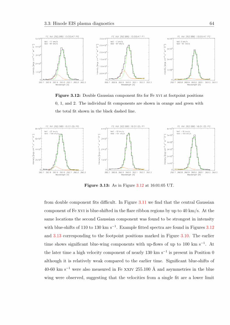
3.3: Hinode EIS plasma diagnostics 64
Figure 3.12: Double Gaussian component fits for Fe xvi at footpoint positions
0, 1, and 2. The individual fit components are shown in orange and green with
the total fit shown in the black dashed line.
Figure 3.13: As in Figure 3.12 at 16:01:05 UT.
from double component fits difficult. In Figure 3.11 we find that the central Gaussian
component of Fe xvi is blue-shifted in the flare ribbon regions by up to 40 km/s. At the
same locations the second Gaussian component was found to be strongest in intensity
with blue-shifts of 110 to 130 km s−1. Example fitted spectra are found in Figures 3.12
and 3.13 corresponding to the footpoint positions marked in Figure 3.10. The earlier
time shows significant blue-wing components with up-flows of up to 100 km s−1. At
the later time a high velocity component of nearly 130 km s−1 is present in Position 0
although it is relatively weak compared to the earlier time. Significant blue-shifts of
40-60 km s−1 were also measured in Fe xxiv 255.100 A and asymmetries in the blue
wing were observed, suggesting that the velocities from a single fit are a lower limit

3.3: Hinode EIS plasma diagnostics 65
for the evaporating plasma at this temperature. In the other Fe xxiv line at 192.028A
strong blends from cooler lines (Fe xi) obscured any line shifts in the footpoints where
the hot emission is weak.
Red-Blue Asymmetry — Double-Gaussian fitting by nature can be susceptible to
creating acceptable but unphysical fits to data. For instance, the fitting method does
not guarantee that the best fit is unique, as a pair of Gaussian profiles can be placed
at many different centroids with widths and intensities that will minimise the chi-
squared. In addition, the decision that there should be two separate components of
plasma is somewhat arbitrary, and placing restrictions on their relative size and position
is adding information that may not represent the true state of the plasma. However,
for spectra where the shifted components are very distinct, placing constraints on each
component’s centroid position based on a judgement by eye will often return sensible
fits. The observed Fe xvi 262A spectra used to produce the fits found in Figures 3.12
and 3.13 did not always have clear shifted components, and the shifted component had
to be constrained to an area in the blue-wing between 262.860A and 263.160A. An
unconstrained fit would for some footpoint pixels result in a large slightly blue-shifted
component with a very small centre component or very broad second components with
little blue-shift. While adding constraints helps remove these artefacts we have in the
following described a method to set the constraints with a more physical basis.
For the three positions of interest, marked on Figure 3.10, the line profiles of Fe
xvi were examined more carefully after developing an alternative method. The signal
was first binned with the 2 pixels above and below in the y-direction to ensure a
high signal-to-noise ratio. Next, we used the Red-Blue Asymmetry method described
in De Pontieu et al. (2009) to find the position of maximum asymmetry within the
line profile. This method was originally used for the detection of transient up-flows
associated with spicules in the quiet sun, and has also been successful in finding high
speed features in the chromospheric network. In our analysis, we start by taking a
single Gaussian fit to the observed line which is plotted on a velocity axis centred with
0 km s−1 at the line centre. Each wavelength now corresponds to a velocity given by

3.3: Hinode EIS plasma diagnostics 66
Equation 3.3. For a velocity interval, δV , the difference between the fit and observed
profile can be compared to that on the opposite side of the fitted centroid, and the
difference used as a measure of the line asymmetry at δV . By measuring the asymmetry
across the profile for a small δV , we build up a profile of the Red-Blue line asymmetry
in velocity space.
Here, in an attempt to improve our fitting, we have used this to find the position
of maximum asymmetry in the line, and then the second Gaussian component is con-
strained to within a limited range of this velocity (wavelength). The aim of this is
to provide the second component with some physical basis to its location without an
a priori assumption. Only the Gaussian widths were further constrained by using a
lower limit equal to the instrumental width. Fitted profiles at the positions marked
on Figure 3.10 for a selection of rasters are found in Figure 3.14. As we have used a
δV = 10 km s−1 we apply an uncertainty of ± 10km s−1 on the measured line shifts.
This δV was chosen as it was small enough to give a smooth asymmetry distribution
while being greater than the minimum Doppler shift that can be measured by EIS. A
larger δV will decrease the precision that the second component can be placed at but
very small values will create a noisy asymmetry distribution which is difficult to obtain
a maximum value from.
In the first row of Figures 3.14 (a) to 3.14 (c), at Position 0, a blue wing asymmetry
is clearly seen compared to the single central component in green. The fitted second
high speed component in orange is surprisingly strong in the earliest raster, and while
reducing in intensity at 16:01 UT moves from up-flows of 100 km s−1 to 140 km s−1.
The centre component is also blue-shifted at 16:01 UT to around 40 km s−1. In Fig-
ures 3.14 (d)-(f) a large 40 km s−1 flow is found in Position 1, but only in the early
raster, and again in Position 2, a faster but weaker flow of 115 km s−1 is found at
16:01 UT but no later. The central component in Position 2 at 16:01 UT is also
blue-shifted, similar to Position 0. At these temperatures the event appears to have a
tendency toward a high speed up-flowing component forming very early in the impulsive
phase, which is later followed by a slower movement of the bulk plasma. Interestingly,
this does not fit a situation where high speed up-flows found at flare footpoints coin-

3.3: Hinode EIS plasma diagnostics 67
cide with stationary background emission such as in Del Zanna et al. (2011), where the
high speed evaporated emission is superimposed on a stationary footpoint. Our result
tends to suggest that the majority of the plasma at this temperature is also, albeit for
a short time, rising. Further analysis would be required to find if this is true at other
temperatures.
To remark on the R-B fitting technique, we find that in general it returns similar
fits and velocity estimates to the simple constrained method used to generate the fits
in Figures 3.12 and 3.13, although there are some differences. For Position 0 the
measured velocities agree to within 5 km s−1 at 15:55:47 UT, however at 16:01:05 UT
the R-B technique fits a high velocity component that is 17 km s−1 faster. For Position
1 the high velocity component is found to be 45 km s−1 slower at 15:15:47 UT. These
differences highlight the influence that setting constraints can have on the resulting
velocity measurements. With no constraint the fits may be unreliable, yet setting limits
by eye can introduce observational biases. The R-B technique addresses this concern
by placing a constraint based on properties of the asymmetric line. In circumstances
where there is considerable deviation between techniques we are thus inclined to trust
the R-B method over fitting using constraints set by eye.

3.3: Hinode EIS plasma diagnostics 68
(a)
(b)
(c)
(d)
(e)
(f)
Figure
3.14:Fexvidou
ble
compon
entfits
usingtheR-B
asymmetry
constraintforthepositionsshow
nin
Figure
3.10.
Thetw
oGau
ssiancompon
ents
ofthefitaremarked
ingreen
andorange,
andthetotalfitbythesolidblack
line.
The
EIS
datais
show
nbythestepped
black
line.
Thevelocities
ofboth
components
are
show
nontheplots
whereVel1
is
greencompon
entan
dVel2theoran
ge.In
thetoprow
theevolutionofPosition0is
show
n,wheretheenhancedbluewing
compon
entis
strongin
thefirstpan
el.In
theother
twopositions,
show
nonthebottom
row,theenhancementis
only
prevalentearlyon
inPosition1an
don
lyjust
noticeable
atPosition2.

3.4: Time Evolution of Selected Footpoints 69
3.4 Time Evolution of Selected Footpoints
The 150s cadence of the raster set, while compromised to provide wider spatial cov-
erage, is sufficient to observe changes in plasma flows and densities during the flare
impulsive phase. The time evolution of plasma parameters from the positions in Fig-
ure 3.10 are shown in Figures 3.15 to 3.18. In each position the fit parameters of
the pixel were averaged with the pixels above and below in the y direction, partly to
improve the signal to noise ratio, and to account for any residual correlation errors.
Pixels were not binned in the x direction, as doing so would sample flux from a 20′′
wide area due to the slit spacing.
Position 0 — The evolution of Position 0 is shown in Figure 3.15, where at 16:01 UT
oppositely-directed flows are immediately apparent, indicating that this is a location
of strong evaporation. The Fe xvi, Fe xiv and Fe xiii lines are all blue-shifted almost
simultaneously, while slight red-shifts on the order of 10 km s−1 appear in the cooler
Fe xii, Fe x, and He ii lines. The up-flow velocity increases with line temperature
above Fe xii, reaching almost 40 km s−1 in the centre component of Fe xvi. As seen
in Section 3.3.3, high speed up-flows of nearly 140 km s−1 are also found in the Fe
xvi blue-wing component at this time, however, as they were only significant in a few
rasters they are not plotted here. Fe xxiv is also blue-shifted by at least 35 km s−1
at 16:01 UT. Clear footpoint emission in the hottest lines was not observed in every
raster so we do not have the data to compare the evolution here.
Given the spectral resolution of EIS, velocities can be measured from centroid shifts
to within ±5 km s−1 (Culhane et al. 2007). However, the accuracy of our chosen rest
wavelength is difficult to quantify, and may introduce a systematic uncertainty in the
results. The quiet area chosen in Section 3.2.2 was selected where the average line
centroid shift compared to the theoretical rest wavelength was close to zero. The
deviation in all pixels was mostly within 5 km s−1. While we can discuss relative
velocity shifts with confidence, we estimate that the absolute velocities could be off by
a maximum of 10 km s−1.

3.4: Time Evolution of Selected Footpoints 70
Figure 3.15: Time evolution of plasma parameters for Position 0 in Fig. 3.10.
The panels show, from left to right, the evolution of the line-of-sight velocity
shift in five iron transitions plus helium, the electron density, and the intensity
including the components of the density diagnostic excited from the ground state.
The velocities shown for Fe xvi are derived from the centre component of the
double fits in Section 3.3.3.
As the velocity shifts peak at 16:01 UT, the electron number density also peaks at
log ne = 10.9 in the Fe xii diagnostic and at log ne = 10.3 (ne in cm−3) in Fe xiv. The
Fe xiii diagnostic used saturates about log ne = 11.3 but due to problems in the atomic
physics may be inaccurate above log ne = 10.3 (Young et al. 2009). Although it appears
to follow the behaviour of the other diagnostics reasonably well, it fluctuates more at
high densities. While the velocities sharply rose at 16:01 UT (also the time of the first
12-25 keV peak), the densities rise more gradually during the impulsive phase. We have
where possible interpolated the upper and lower limits of the measured intensity ratios
onto the density curve, returning the possible range of electron densities, however,
these do not include errors in the atomic physics calculations which may account for
more systematic variations.
The intensities of the spectral lines excited from the ground state are enhanced
significantly between 15:55 UT and 16:01 UT. The mid-temperature lines, between Fe
x and Fe xiv, peak at 15:55 UT with Fe xvi rising a few minutes later. The very steep

3.4: Time Evolution of Selected Footpoints 71
Figure 3.16: Intensity variation of transitions to the ground state in the di-
agnostic pairs (solid lines) and the same intensity divided by the square of the
measured density (dotted lines).
rise in the cool He ii line can often be associated with the time of energy deposition
and HXR emission of the flare. This event is no different, and the earlier 12-25 keV
peak is matched by the He ii rise.
As mentioned earlier in Section 3.3.1, the intensity of the allowed transitions in the
diagnostic pairs is proportional to n2e. If a cool plasma of constant density were to be
heated, any allowed transition with a formation temperature Tmax would brighten as
more plasma is heated to Tmax. Our diagnostics show that the density is increasing.
If the plasma were to be at constant temperature, the intensity would rise with n2e.
Any additional increase may be interpreted as a temperature rise in the local plasma.
In Figure 3.16 the intensity for the transition excited from the ground state for diag-
nostic pairs is plotted, and the same intensities are shown divided by the measured
n2e to remove the density proportionality — an arbitrary constant is added to display
them together. The resulting time profiles are remarkably flat with only very small
variations, thus the intensity change can almost be entirely attributed to the change
in density with very little temperature change.

3.4: Time Evolution of Selected Footpoints 72
Positions 1 & 2 — The other two footpoints are similar in character but with some
key differences. The electron density at Position 1 (Figure 3.17) located on the southern
side of the filament reaches the highest seen during the flare, rising to log ne = 10.3
in Fe xiii and Fe xiv, and to log ne = 11 in Fe xii. However, the hot lines while
blue-shifted do not display the same well defined shifts as at Position 0. He ii and
Fe xii are only slightly red-shifted at 16:01 UT. There is some evidence of a higher
speed up-flow present in Fe xvi of 42 km s−1 (Figure 3.14) at 15:55 UT but the centre
component is not significantly shifted at 3 km s−1. Fe xxiv also has no strong signal
here.
Finally, Position 2 (Figure 3.18) is where a density enhancement in the southern
ribbon first arises, eventually forming the ‘U’ shaped density enhancement south of
the filament. Measured densities do not appear to rise until after 15:55 UT where all
three diagnostics suddenly jump in density, with Fe xiv showing log ne = 10.2, with
log ne = 10.8 in Fe xii. The rapid rise in density can possibly be explained by the
scanning slit passing over the edge of the flare kernel, which may be smaller than the
10′′ raster spacing. Again there are significant up-flows in lines hotter than Fe xiii but
only to speeds of around half that of Position 0. Simultaneous red-shifts are present
at this position in Fe x and He ii on the order of 5-10 km s−1. Although weaker than
at Position 0, here we see Fe xvi blue-wing flows of 115 km s−1.
We can summarise this somewhat exhaustive list of observations with three key
points: (1) electron densities are increasing across all of the EUV footpoint regions
during the flare impulsive phase, (2) we deduce that the apparent density rises in
the footpoints, although while the footpoints are being heating, the temperature does
not appear to be contributing to the diagnostic line intensities, and (3) high speed
evaporative up and down flows are seen in at Positions 0 & 2, while Position 1 exhibits
very little plasma motion, but has the same enhanced electron density.

3.5: RHESSI data analysis 73
Figure 3.17: As in Fig. 3.15 but showing parameters for Position 1
Figure 3.18: As in Fig. 3.15 but showing parameters for Position 2
3.5 RHESSI data analysis
RHESSI X-Ray observations are the final piece of this multi-wavelength puzzle. In
the thick-target model of flare energy deposition, accelerated electrons lose energy and
heat the chromosphere through Coulomb collisions. The presence of these electrons is
detected observationally by a HXR non-thermal power-law component of the photon
spectrum. If we assume the footpoint heating is driven by these electrons, then the
energy flux deposited in the chromosphere can be estimated from the HXR spectra
(Section 1.3.1). RHESSI is also capable of imaging the location of HXR emission using

3.5: RHESSI data analysis 74
techniques discussed in Section 2.4.5, which will determine if the energy deposition is
occurring at the same location as our EUV footpoints.
Figure 3.19: Impulsive phase TRACE 171 images with RHESSI 60%, 80%
and 90% intensity contours overplotted in 6-12, 12-18 and 18-25 keV energies
(magenta, green and yellow respectively).
The RHESSI data preparation and spectral fitting described here was performed
by I. Hannah in Graham et al. (2011). The times for spectral analysis in RHESSI were
chosen to match the two peaks in the 12-25 keV emission whilst avoiding periods when
the A1 attenuating shutters were in place. These shutters are at times placed in front of
the germanium detectors to prevent what is known as pulse-pileup. This is an artefact
found at high photon fluxes, caused when a second photon arrives in the detector before
the energy of the first has been processed. The result is that both are read as a single
photon with their combined energy. The data was background subtracted using a level
taken from during an eclipse period, where the X-ray flux is at its lowest. The RHESSI
images were produced using counts from detectors 3, 4, 5, 6, and 8 using the CLEAN
algorithm. Detector 1 had the best energy resolution and lowest background during
this pre-anneal time and was selected to perform the spectral analysis (an anneal is
a heating procedure carried out every few years to help remove crystal defects in the
RHESSI germanium detectors, which reduce their efficiency. Doing this ensures the

3.5: RHESSI data analysis 75
detector response is uniform (Hannah et al. 2010)). The OSPEX package was used to
fit a thermal (Maxwellian) plus thick-target non-thermal model (Section 1.3.1) to the
spectral data. The CLEAN algorithm and OSPEX package were discussed in Section
2.4.5.
Imaging — The difference in pointing between TRACE and RHESSI is unknown,
making aligning the HXR image onto the EUV emission difficult, but it is possible
to align the images via other instruments. We have used continuum images from the
Michelson Doppler Imager (MDI) on board SOHO and also white light (WL) images
from TRACE to align the RHESSI imaging. The pointing for SOHO/MDI is well
known as it is centred on the solar disc. RHESSI can also very accurately find the
limb with its aspect sensors which allows it to be co-aligned with MDI. The MDI
continuum and TRACE WL images also display the same features, and these can be
cross-correlated to find the residual pointing difference between TRACE and the solar
disc centre, which we assume equates to the pointing difference between RHESSI and
TRACE. Since the TRACE 171A images should be aligned with the TRACE WL
images, both the TRACE 171A and RHESSI HXR images can be aligned.
MDI continuum is only available a few times a day, in this case at 12:29 UT, while
the closest TRACE WL image to the flare peak was at 15:31 UT. The MDI image
was rotated using the SolarSoft drot map software to account for the solar rotation
between these times. Their offset was found using the cross corr routine with some
manual adjustment, and as SOHO is positioned at the L1 Lagrange point, a further
correction for the Earth parallax shift of the TRACE orbit was required. Spacecraft
drift between TRACE 171 A images was corrected for by tracking the movement of
stable bright points north of the filament using the same procedure as the EIS rasters
(Section 3.2.2). After these corrections, we estimate the pointing of TRACE with
respect to RHESSI to be within 1.5′′ in each direction.
The results for two RHESSI images at times corresponding to the 12-25 keV peaks
are shown in Figure 3.19. The RHESSI contours for three energy bands, 6-12, 12-18,
and 18-25 keV, lie on top of bright TRACE 171 A regions which we associate with chro-

3.5: RHESSI data analysis 76
mospheric emission. The HXR emission is localised in the southern ribbon area, yet
surprisingly there is no evidence for a HXR footpoint at Position 0 (Figure 3.15) north
of the small filament. Position 0 showed the most convincing chromospheric evapora-
tion signatures of the positions studied, along with strong density enhancements, yet we
see that the HXR sources are found in the southern ribbon, where evaporation signa-
tures are weaker. An offset of ∼ 20′′ between the TRACE and RHESSI images would
be necessary to align RHESSI sources with Position 0. Given our careful co-alignment
process, we believe that such an error in relative pointing is unlikely. Furthermore, the
shape of the HXR footpoints seen match well with the TRACE emission. This implies
the energy input from non-thermal electrons must be relatively weak here compared
to the southern region, if indeed that is what is driving the evaporation. It should
be noted that we use the term ‘hard’ X-ray here loosely. The two impulsive bursts of
12-25 keV emission under the slow rising GOES SXR curve are characteristic of emis-
sion from non-thermal electrons, but compared to the electron spectra found in larger
flares (where footpoints are seen at much higher energies) the distinction between non-
thermal and thermal components is not obvious as will be seen in the spectra below.
Spectra—When the incoming photon flux is high RHESSI is capable of reconstructing
the photon spectra from individual footpoint areas. The count rate in this event
however was relatively low, so the spatially integrated photon flux was used to create
the spectra found in Figure 3.20. The spectra corresponding to both images in Figure
3.19, both peaks of the 12-25 keV light curve, are shown in the top and bottom panels
of Figure 3.20. For each time step the photon spectra was fitted with two models; a
thick-target model single power-law plus a single thermal component, and with a pair
of thermal components. The thick-target fit returns the best fit parameters describing
the bremsstrahlung photon spectra for non-thermal electrons interacting via Coulomb
collisions with the background chromospheric plasma (Brown 1971; Holman 2003). The
fit uses an accelerated electron distribution of the form f(E) ∝ E−δ, where delta is
the electron spectral index. The total electron number flux, Ne, of the incoming beam
is thus given by Ne =∫ Ehigh
ECf(E)dE, where EC is the electron low energy cut-off.

3.5: RHESSI data analysis 77
The high energy cut-off, Ehigh, while used to constrain the problem, does not have a
significant effect on the fit and is not shown in the following discussion. Each thermal
fit gives the photon spectra emitted by electrons in a thermal Maxwellian distribution,
described by the total emission measure, EM , and the core temperature, T . The fitted
parameters for the spectra shown are found in Table 3.2, and further details on the
production of bremsstrahlung X-ray spectra, their fitting, and fit parameters are found
in Section 1.3.1.
The background level for this event (plotted in grey) is elevated due to degraded
detector performance at this time. The outcome is that the non-thermal component,
shown in blue on the left hand plots of Figure 3.20, is not particularly clear at high
energies (above 20 keV). However, the thermal + non-thermal fit here is considerably
closer than the single thermal fit (red line) above ∼ 12 keV, which breaks away con-
siderably from the data. The spectral index varies slightly between 9.3 and 9.7 for the
earlier and later times, suggesting that while the second 12-25 keV peak was larger in
flux, the spectra was ‘harder’ earlier in the flare, leading to more footpoint heating and
evaporation. The photon energy above which the spectrum can be referred to as non-
thermal is parameterised in the fit by the cut-off energy EC. Labelling this transition
with a hard cut off is somewhat un-physical, as the spectrum represents a continuous
distribution of energies, however, it does represent the most probable photon energy
that originates from the accelerated electrons. In these fits EC ∼ 16keV for both times
during the event.
In the right hand of Figure 3.20 plots we show the double thermal component
fits. The reasoning behind this came from the referee for Graham et al. (2011), who
suggested that given the relatively soft X-ray spectra observed, a pair of thermal com-
ponents may be better fit the observations — this would imply the flare heating was
not directly the result of accelerated electrons. A pair of thermal components (red and
orange lines) does appear to provide an acceptable fit to the data as seen in the plots,
but again the high background level makes it difficult to determine at higher energies.
The higher temperature thermal component (orange line) drops away from the data at
high energies slightly more than in the non-thermal model (blue line). However, visu-

3.5: RHESSI data analysis 78
10Energy [keV]
10-2
100
102
104
Pho
ton
Flu
x [s
-1 c
m-2 k
eV-1]
16:02:40 +60sχ2=2.0
10Energy [keV]
10-2
100
102
104
Pho
ton
Flu
x [s
-1 c
m-2 k
eV-1]
16:02:40 +60sχ2=2.1
10Energy [keV]
10-2
100
102
104
Pho
ton
Flu
x [s
-1 c
m-2 k
eV-1]
16:09:52 +60sχ2=1.8
10Energy [keV]
10-2
100
102
104
Pho
ton
Flu
x [s
-1 c
m-2 k
eV-1]
16:09:52 +60sχ2=1.9
Figure 3.20: RHESSI photon spectra times corresponding to the first (top)
and second (bottom) 12-25 keV peak. The data for both peaks is fitted with
two models: in the left hand panels, a single thermal component (red) plus thick
target model of accelerated electrons (blue); and in the right hand panels, a pair
of thermal components (orange and red).
ally, and even from the χ2 values, all between χ2 = 1.9− 2.1, there is little evidence to
favour one model over another. Nevertheless, the implications of both are discussed in
the next section.
Looking back at the morphology of the RHESSI contours in Figure 3.19, the earlier
frame appears more consistent with hot footpoint emission. Two regions of similar size
to the patchy bright regions in TRACE lie in the 6-18 keV energy range. From both
spectral fits, we find that at energies up to 12 keV the emission is dominated by a
hot thermal component at around 16 MK; the central concentration of SXR emission
in Figure 3.5 confirms this picture for plasma with a temperature of at least 8 MK.
Interestingly, the imaging at this time showed no sources between 18-25 keV. In the

3.5: RHESSI data analysis 79
later frame, the emission is less localised, possibly outlining the shape of a loop at
6-12 keV, yet the concentration at 18-25 keV hints at a footpoint contribution from
below, and is at the location of the largest density enhancement (Position 1).

3.5: RHESSI data analysis 80
Table
3.2:Model
param
etersfortheRHESSIphotonspectrum
at16:02UT
and16:09UT.Parametersforboth
thermal
plusthick-targetan
ddou
ble
thermal
fits
areshow
n.EM
andT
are
theem
issionmeasure
andcore
temperature
ofeach
thermal
compon
ent,δis
theelectron
spectral
index,E
Ctheelectronlow
energycut-off,andN
etheelectronnumber
flux.
Fit
Tim
eEM
1EM
2T1
T2
δE
CN
e
(104
8cm
−3)
(104
6cm
−3)
MK
MK
(keV
)(103
5electron
ss−
1)
Th×2
16:02:40
0.6±
0.1
4.3±
0.9
15.7±1.0
27.0±
0.8
...
...
...
Th+
TT
16:02:40
6.8±
0.2
...
16.4±1.1
...
9.3±0.4
15.6±
0.6
2.7±1.0
Th×2
16:09:52
1.7±
0.5
8.5±
2.3
14.3±0.8
25.9±
0.9
...
...
...
Th+
TT
16:09:52
1.3±
0.3
...
16.2±0.6
...
9.7±0.3
16.5±
0.5
2.6±0.7

3.6: Processes taking place at the flare footpoints 81
3.6 Processes taking place at the flare footpoints
The observational parameters that describe the flare energy input flux in the footpoints
have now been estimated, along with diagnostics of the plasma heating and dynamic
response to the energy flux. We are now in a position to investigate how our new
observation, that electron densities at the footpoints during the impulsive phase are
enhanced, ties in with our current understanding of flares. The observations can be
summarised as follows. During the impulsive phase, energy is deposited into a number
of small regions in the chromosphere/transition region, visible as ribbons and footpoints
in UV and EUV, and also in SXR images, implying that the plasma is at low heights
but heated to temperatures of a few MK. Hinode/EIS iron density diagnostics formed
at around 1.5 MK show the electron density increases here during the early impulsive
phase, typically up to a few times 1010cm−3, but since the ground state transition only
increases slightly beyond its n2e dependence, we infer that any variation in temperature
of the plasma emitting these lines is small. A number of the footpoints show line-
of-sight velocity shifts during the impulsive phase — on the order of 20-140 km s−1
— at the time of the ne enhancements, and with a tendency for lines cooler than
Fe xiii to be red-shifted and those hotter to be blue-shifted. These are followed in the
gradual phase by substantial red-shifts in most lines, associated with the draining of
hot material. Unexpectedly, the footpoint showing the strongest impulsive-phase line
shifts (Position 0 in Figure 3.10 and regions north of the filament) does not have any
detectable RHESSI source. This last point, and the high observed densities, are two
of the questions that we will try to answer.
What process is leading to the increasing ne values? The most straightforward
explanation is to assume that the observed iron emission is emitted primarily by plasma
at the temperature of maximum ionisation fraction, Tmax, of the relevant ion, and that
during the flare impulsive phase deeper layers of the atmosphere are heated to this
temperature. Correspondingly, the dominant emission will originate from regions of
increasing density, but always at around Tmax. The small increase in intensity of the
ground state transition beyond the density proportionality (see Figure 3.4) does suggest

3.6: Processes taking place at the flare footpoints 82
that there is a small contribution to the line intensity in addition to dominant effect of
heating denser layers. We interpret this as heating of plasma in different layers within
the same optically thin column. A second case for a density enhancement would be
to assume a scenario whereby already hot plasma at a depth in the transition region
is compressed resulting in a higher density, such as in the case of a downward moving
conduction front driving evaporation (Fisher 1989). However, in this case the location
of the front is still moving to regions of higher density and these two effects may be
difficult to separate diagnostically.
Modelling of gentle evaporation, and of the gentle early phase of a flare which
later displays more explosive evaporation caused by an electron beam (Fisher et al.
1985; Allred et al. 2005), shows that the position of the transition region (i.e. the
location of rapid increase in atmospheric temperature) moves downwards slightly in the
atmosphere and the density just below the transition region increases, which is roughly
consistent with what we see here. Although the majority of the velocity shifts observed
in this small event are fairly low compared to similar events (Milligan & Dennis 2009;
Watanabe et al. 2010), the presence of high speed flows in Fe xvi suggests that there
is some dynamic plasma motion here consistent with more explosive evaporation (the
difference between gentle and explosive evaporation is detailed in Section 1.3.2). In
the model found in Fisher et al. (1985), a transition between gentle and explosive
evaporation is found at non-thermal input fluxes of around Fp ∼ 1010 ergs cm−2 s−1.
We calculate this flux via the RHESSI spectra in the next section and attempt to
explain the evaporation characteristics. However, it should be noted that the existing
models often use input electron spectra that are much harder and typically have a
higher cut-off energy than we infer from HXR measurements, so that the majority of
collisional energy input occurs deeper in the atmosphere. Direct comparisons of our
results with these models may not always be reliable.
The diagnostics show that ne increases typically to a few ×1010cm−3 while the high-
density sources remain compact (i.e. not loop-like). This places the emission location
relatively low in the atmosphere. In a non-flaring (but still active) atmosphere, for
example the VAL-E model for bright network (Vernazza et al. 1981) appropriate for

3.6: Processes taking place at the flare footpoints 83
the active region locations where the flare occurs, a density of ne ∼ nh = 4×1010 cm−3
occurs at a column depth of 5.8 × 1018 cm−2, where the hydrogen ionisation fraction
is approximately equal to unity. In some instances, for example the Fe xii diagnostic
at Position 1, ne approaches 1011 cm−3, which corresponds to regions in the VAL-E
atmosphere where the plasma is only partially ionised. In such cases, it is possible
that an electron beam, containing sufficiently high energy electrons, could lead to an
increase in the observed electron number density due to collisional ionisation, followed
by heating. To do this, the electron beam must be able to penetrate to regions where
ionisation fraction is less than one — in the VAL-E model the ionisation fraction drops
off at depths below around 2000 km in the chromosphere. We clearly see heating at
chromospheric heights in this event, and in a thick target regime, as we show below,
we find that driving ionisation at these depths is not a demanding condition. In the
next few sections we use the RHESSI fit parameters in a quantitative manner to verify
if these observations can be explained by electron beam heating or otherwise.
3.6.1 Electron Stopping Depth
The depth at which a non-thermal beam of electrons is stopped in the chromosphere
can estimated from the collisional thick target model. Starting from the equation found
in Emslie (1978), the stopping depth, Nstop, of an electron of energy E and speed v
can be found using the following expression
dE
dN=
−2πe4
E[xΛ + (1− x)Λ′]nHv , (3.4)
where Λ is the Coulomb logarithm, Λ′ is the associated Coulomb logarithm, and e
the electron charge. In this case the target plasma is hydrogen of total number density
nH and ionisation fraction x. The Coulomb logarithms, electron velocity, and ionisation
fraction are functions of the column depth N and electron energy, hence it is not
straightforward to integrate to find the stopping depth. This expression was integrated
computationally by L. Fletcher in Graham et al. (2011) to find the stopping column
depth as a function of the initial electron energy, and is shown in Figure 3.21 using

3.6: Processes taking place at the flare footpoints 84
Figure 3.21: Stopping column depth as a function of the injected electron energy
for the VAL-C and VAL-E model atmospheres. The depth at which the VAL-E
atmosphere is 10% and 50% ionised is shown by the horizontal lines.
parameters from the VAL-C and VAL-E models. As expected electrons with a higher
input energy travel further into the chromosphere before being stopped by collisions.
Horizontal lines on Figure 3.21 indicate the approximate locations at which the VAL-E
atmosphere is 50% and 10% ionised. With the value of EC, found from the RHESSI
fitting, of 15.6 keV the beam energy is mostly deposited around 5 − 10 × 1019cm−2.
Electrons of this energy will easily penetrate to depths where the atmosphere is partially
ionised (almost neutral) and have the potential to increase the hydrogen ionisation
fraction. The increased free electron count may contribute to the electron densities
found via the diagnostics, but without further calculation it is unclear by how much,
and how long the plasma can remain out of equilibrium at high density (see Section
2.1).

3.6: Processes taking place at the flare footpoints 85
3.6.2 Electron Beam Power
The total power deposited by a beam of accelerated electrons can be calculated from
parameters of the X-ray photon spectra fit. In the thick-target interpretation this
energy is assumed to be delivered into the chromosphere and is the source of the
flaring processes that we see. In Section 3.5, the RHESSI photon spectrum was fitted
with a collisional thick-target model for accelerated electrons. The accelerated electron
distribution could be described as f(E) ∝ E−δ, where δ is the spectral index and the
total number flux of electrons is given by Ne =∫
f(E)dE electrons s−1. The best
fit parameters for the observed spectra were shown in Table 3.2. It can be shown that
the total power in the beam is given by
P =
∫f(E)EdE = 1.6× 10⁻⁹NeEC
δ − 1
δ − 2, (3.5)
where EC is the electron cut-off energy and the power is in units of erg s−1 (see
Holman et al. (2011)). Using the fitted parameters shown in Table 3.2 the equation
returns a power in the non-thermal electrons at 16:02:40 UT of (7.7±2.9)×1027 ergs s−1
and at 16:09:52 UT (7.8 ± 2.2) × 1027 ergs s−1. Both times return very similar power
values and which suggests that the energy deposition rate was similar at both times.
The power per unit area, FP , is a useful measure which can be obtained by es-
timating the HXR source size. Measuring footpoint sizes from RHESSI imaging can
be notoriously uncertain, due to the way in which images are reconstructed, however,
the CLEAN algorithm is capable of resolving sources down to 2′′ where the count rate
is good. In our event the brightest EUV footpoints do appear to be compact, and
are comparable in width to the 12-18 keV sources found in both panels of Figure 3.19,
therefore we estimate the size of these sources to be approximately 5” wide. The higher
energy source (18-25 keV) is slightly more compact, so we suggest that the majority
of the beam power is delivered to an area with an upper limit of 5” x 5”, giving a
footpoint area of 1.3× 1017 cm2. If we use the power from the 16:02 UT spectra, since
it corresponds better with the peak velocity flows, we find that the power per unit area

3.6: Processes taking place at the flare footpoints 86
is FP = 5.9± 2.2× 10¹⁰ ergs cm−2 s−1 for electrons above the cut-off energy 15.6 keV.
The uncertainty in this value is found by propagating the errors from the fit parameters
in Table 3.2. Although the fitted uncertainties in EC and δ are small, as the power
in electrons above the cut-off energy EC depends on E2−δC (since Ne ∝ E1−δ), and the
spectral index is very steep; a small increase in the low-energy cut-off value can change
the power derived by a significant factor.
So through the parameters found by spectral fitting we have arrived at a beam
power leading to energy fluxes of FP ∼ 1010 ergs cm−2 s−1, comparable to those above
which explosive evaporation occurs in modelling (Fisher et al. 1985). However, at the
same time there is sufficient uncertainty in our results, should the source size be larger
or EC higher, that they may also be consistent with a case of gentle evaporation. We
can also consider this uncertainty with respect to the footpoint at Position 0. As we
mentioned in the previous section, the footpoint here displays no clear HXR source,
yet harbours high speed evaporation flows at high temperatures. The dynamic range
of RHESSI is only around a factor of 10, meaning that in a single image, features
with a brightness of less than 10% of the strongest feature will not be observed. If the
uncertainties in FP were to allow for a factor of 10 increase, then if we reduced the FP
value at Position 0 corresponding roughly to RHESSI’s dynamic range, it would bring
the footpoint within the modelling requirement for explosive evaporation, although this
would be stretching the observational limits rather far. By changing the footpoint size
alone, a width of ∼ 1.6′′ would be sufficient to raise FP by a factor of 10, although
such small source sizes may not be unreasonable (see Battaglia & Kontar (2011) and
Battaglia et al. (2012)). Nevertheless, we first we must consider if the flow speeds are
indeed characteristic of explosive evaporation.
3.6.3 Flow Speeds
One of the requirements for explosive evaporation is that the flow speeds are faster
than the local plasma sound speed, as will occur if the heating time scale is shorter
than the hydrodynamic expansion time scale. We can compare the spectroscopically-

3.6: Processes taking place at the flare footpoints 87
determined line-of-sight flow speeds observed in Figures 3.15 to 3.18 to the relevant
sound speed Cs via the expression
Cs = 9.79× 10⁵(γZTe
µ
) 12
, (3.6)
where for ionised hydrogen the atomic number is Z = 1, the adiabatic index γ = 53,
and µ = mi/mp = 1. Taking the temperature of formation of the Fe xiii line as
Te = 1.58 MK, the sound speed of the plasma is cs = 147 km s−1, and for Fe xvi
cs = 185 km s−1. Our observational upper limit of 140 km s−1 for Fe xvi is lower than,
though reasonably consistent, with these speeds. What is perhaps best demonstrated
by these findings is that in a flare of relatively small energy such as this, there is no
clear cut case for either evaporation scenario with the input flux being on the border
of driving both cases. What we have learned though is that the locations of enhanced
density are also sites of evaporation, and the densities are high at the transition between
downward and upward flows — this point will be returned to in Chapter 4.
3.6.4 Electron Beam Heating
To produce the observed iron line emission requires heating the chromospheric plasma
from its ambient state to around 1.5 × 10⁶ K. If we start from the VAL-E model
atmosphere, which we assume to be a reasonable pre-flare atmosphere, the temperature
at a density of a few ×1010cm−3 is around 20,000 K. From Equation (36) in Emslie
(1978) we can estimate the heating rate per target particle for a collisional thick target
beam. At a column depth N the heating rate due to a beam electrons above Ec in a
fully ionised hydrogen plasma is given by
Q = πΛe4(δ − 2)B
(δ
2,1
3
)FP
E2C
[6πΛe4N
E2C
]−δ/2
ergs s−1, (3.7)
where B is the Beta function. By inserting the fitted values for δ and EC, and using
N = 5.8× 1018cm−2 (where ne ∼ 4× 1010cm−3 in the VAL-E atmosphere) we find that
our derived input flux yields a heating rate per particle of Q ∼ 7.8× 10⁻⁶ erg s−1.

3.6: Processes taking place at the flare footpoints 88
At this density, and by using a value from the radiative loss function of Martens et al.
(2000) at around log T = 6.2, f(T ) ∼ 10−21 ergs s−1 cm3, we can estimate the radiative
energy loss rate per particle, which is given by nef(T ) = 4 × 10⁻¹⁰ erg s−1. The con-
ductive energy loss rate per particle can also be estimated by ∼ 10−6T 7/2/neh2 (Spitzer
1962). If we use a temperature T ∼ 2×10⁶ K, and an approximate scale height for the
transition region, h ∼ 107 cm, then the loss rate is approximately 2 × 10⁻⁹ ergs s−1.
The incoming heating flux is therefore well in excess of both of these loss rates, and
clearly the plasma will heat quickly.
3.6.5 Thermal Heating
If we consider the double thermal fits in Figure 3.20, where the spectrum is modelled
by a high and low temperature component, the fit parameters (Table 3.2) suggest that
we see around 5% of the plasma at a temperature of 26 MK. The emission measure in
the hot component at 16:01 UT is around 5× 1046 cm−3, and using the same footpoint
size estimate, we find the column emission measure is ∼ 4× 1029 cm−5. Knowing that
the column emission measure is ne2h, and assuming a constant density of 5×1010 cm−3,
we find that the thickness of the emitting region should be around 1500 km — on the
order of the thickness of the chromosphere. It is slightly unrealistic to assume that
the entire chromosphere is heated to this temperature, but our chosen density gives a
very conservative estimate of the entire thickness. Increasing it to 1011 cm−3 returns a
thickness of around 380 km, comparable with the idea of a thin heated slab in the upper
transition region, cooling by conduction into the lower atmosphere (see the discussion
in Chapter 4). Again this may be viable where the electron cut-off energy is low, since
electrons will be stopped higher in the transition region where it is easier to heat to
the high temperatures observed.
If we continue along this line of reasoning, the conductive flux from a plasma at a
temperature T can be expressed as
Fc = κT 5/2dT
dhergs cm−2 s−1, (3.8)

3.7: Conclusions 89
where κ = 10−6 ergs K−7/2 cm−1 s−1 (Spitzer 1962). If the temperature gradient
dT/dh is assumed to be the difference between the implied 26 MK second thermal com-
ponent and 20,000 K pre-flare atmosphere, taken over the estimated 1500 km chromo-
spheric emitting region, the conductive flux is found to be FC ∼ 6×10¹¹ ergs cm−2 s−1.
This is sufficient to drive explosive evaporation, according to modelling, by an order
of magnitude. The estimate is very much an upper limit, as we have assumed that
classical conductivity applies (see Section 4.6), that energy losses from flows and radia-
tion are negligible, and that the density is constant throughout the region, although it
does demonstrate that there could be a significant energy flux present from conduction
alone. These numbers give us some explanation to the absence of HXR sources at the
strong evaporation sites, however, the transition region still requires heating to high
temperatures via some energy release. The conclusion drawn from morphology of the
X-ray sources discussed in Section 3.5 was that of compact footpoint sources, with
little evidence for a hot loop connecting the strong evaporation site (Position 0) to the
RHESSI sources. If the RHESSI sources were that of a hot loop top, the fainter loops
seen in XRT could in theory conduct heat to the northern region. Recalculating the
flux using a loop length of 20′′ gives Fc ∼ 6 × 10¹⁰ ergs cm−2 s−1, which is still com-
parable to the non-thermal beam case. Yet without clearer observations we still can
not be certain of either case, and a combination of both conductive and non-thermal
heating is likely, nonetheless it is worth exploring all avenues that these observations
allow for.
3.7 Conclusions
The initial objective of this analysis was to obtain an estimate for the footpoint elec-
tron density during the impulsive phase using data from Hinode/EIS. After finding an
event which had excellent coverage in a number of instruments, it quickly led on to ex-
ploring the physics that could be extracted from so many co-aligned multi-wavelength
observations. In this chapter we have shown that Hinode/EIS imaging spectroscopy
is capable of capturing the evolution of compact flare footpoints during the impulsive

3.7: Conclusions 90
phase, and that along with many supporting observations, diagnostics can be made
of the plasma which are reasonable in the scheme of recent modelling of flare energy
deposition and can question which models are most suitable for small flares.
We found through a detailed application of Hinode/EIS spectral diagnostics ev-
idence for an increase in flare footpoint plasma density emitting at temperatures
∼ 1.5 − 2 MK, and at depths which are consistent with a downward motion of the
transition region during gentle evaporation. RHESSI X-ray spectroscopy, interpreted
using the collisional thick-target model, placed limits on the energy flux of an electron
beam producing the observed flare chromospheric heating. Combined with an estimate
of the RHESSI non-thermal source size, the derived beam power per unit area was in
excess of that which should lead to explosive evaporation, though a very soft spectrum
and uncertainties in the low energy cut-off make the result somewhat speculative. We
therefore considered an alternative double thermal model, which fits the data equally
well, and may feasibly explain the observed evaporation site with no HXR source by
implying heating through a conduction flux. However, the imaging at two periods in
the impulsive phase suggests the HXR emission is dominated by footpoint sources and
not loop structures heated to flare temperatures.
Diagnostics of this nature are clearly extremely important in determining the re-
sponse of the lower atmosphere during flare heating to various energy input methods.
The results within this chapter may be fairly inconclusive, but have explored and re-
fined diagnostic techniques which can be focused on observations with better spectral
coverage, as will be seen in the following chapters.

Chapter 4
Impulsive Phase Flare Footpoint
Emission Measure Distributions
In this chapter, we have furthered the investigation of footpoint heating by employing
a new technique to recover the first emission measure distributions (EMD) of impul-
sive phase footpoint plasma using Hinode/EIS data, allowing us to view the emission
measure as a function of temperature with excellent spatial resolution. The bulk of
the work in this chapter was published in Graham et al. (2013) for 6 flares occurring
during a period between May and December 2007. What is presented here describes
the same analysis but provides more insight in interpreting the results and testing the
inherent assumptions.
During the impulsive phase of a solar flare, the temperature distribution of the
heated footpoint plasma provides a critical constraint on the distribution of energy
injected from the flaring mechanism. When heating a stratified pre-flare atmosphere,
the depth in the atmosphere of energy input, methods of energy transfer within the
plasma, and magnitude of the input energy flux will all have an effect on the footpoint
temperature distribution. Our motivation was thus, if the recovered EMDs were suf-
ficiently robust, i.e. more sensitive to changes in the plasma than the uncertainties
in the method, we could make comparisons with EMDs calculated from modelling to
infer what physics is involved in the observed heating.

92
Prior to our analysis, this observable had never before been measured using an
instrument with as high spatial and spectral resolution as EIS; although several studies
had been made with EUV data from instruments onboard the Skylab space station
(see Tousey (1977) for an overview), the results were somewhat compromised by the
instrumental limitations at the time. We find that our EMDs derived from EIS give
a clearer picture of the heated flaring atmosphere, however, though they supersede
the earlier work we find our results from EIS are comparable to some of the EMDs
extracted from the Skylab data. We compare our EIS EMDs with these prior results in
more detail in Section 4.5.1 and 4.6, finding the slope of the EMD to be an important
diagnostic tool.
In our analysis of EIS footpoint data, the EMD is obtained from intensity mea-
surements across a wide range of temperatures in conjunction with knowledge of the
emission line contribution functions. In our analysis we have used a regularized inver-
sion method developed by I. Hannah (Hannah & Kontar 2012) — adapted from the
inversion of RHESSI HXR spectra — which inverts the key equation
I =
∫G(T, ne)ξ(T )dT (4.1)
to find the differential emission measure, ξ(T ), in the form
ξ(T ) = n2e
dh
dTcm−5 K−1. (4.2)
We use observed EIS line intensities, I, and the contribution functions, G(T, ne),
from CHIANTI v7.0 (Dere et al. 1997; Landi et al. 2012) in order to perform the in-
version and find ξ(T ) which gives us the EMD(T). The distinction between DEM and
EMD is clarified in Section 4.1 and full details of the inversion method are found in
Section 4.4.
Even though interpreting EMDs can be notoriously ambiguous (Brown et al. 1991;
Judge et al. 1997; McIntosh et al. 2000), the resulting temperature distribution is ex-
tremely useful. For example, in our analysis it was immediately clear that the plasma

4.1: Secrets of the EMD 93
is not isothermal, and that a distribution exists which must result from some temper-
ature gradient. We have taken steps to ensure that physics extracted from our EMDs
can be trusted: 1) by using line intensities that are spatially resolved and de-blended;
2) by using an inversion method that returns EMD uncertainties and makes no a pri-
ori assumptions about the plasma; 3) by testing the method on various solar features;
and finally 4) by understanding the assumptions inherent in the atomic physics. From
our analysis and comparing to theoretical models we have concluded that the result-
ing EMDs are compatible with an atmosphere heated by non-thermal electrons in a
relatively thin, hot layer, which then transfers energy via conduction into cooler layers
emitting the observed EUV radiation. We find that the technique allows one to learn
about the energy transfer within the plasma column, and of the thickness of heated
regions — a parameter which is not always readily available from line of sight optically
thin EUV observations.
4.1 Secrets of the EMD
As mentioned the EMD can provide an observational description of the plasma prop-
erties of the lower atmosphere footpoints of solar flares and is a critical constraint on
the distribution of the flare excess energy in this region, and hence the profile of flare
energy deposition and its possible modes of transport. In the previous chapter we
saw that the temperature coverage of EIS makes it extremely well suited to studying
heated footpoint plasma and that we find evidence for temperatures on the order of
8 MK present in the lower atmosphere. To determine the EMDs we take advantage
of the EIS temperature range to find the temperature distribution of emitting plasma
from 250,000 K to over 10 MK.
4.1.1 DEM to EMD
Before going any further this is a good place to make the distinction between the
differential emission measure (DEM) and emission measure distribution (EMD). It

4.1: Secrets of the EMD 94
is a simple point, but is often overlooked and important when making comparisons
between the results of different authors. The DEM, as defined above, arises from the
mathematics shown in Section 2.3 and is a function of the emitting material weighted
by the inverse temperature gradient. The inversion method used will return ξ(T ) and
has the units cm−5 K−1 for a plasma column of unit area.
The quantity ξ(T ) is physically not very illuminating on its own. We can there-
fore integrate ξ(T ) over the width of each temperature bin to give the total emission
measure within a small temperature range ∆T as a function of temperature. This also
helps when comparing to results where the EMD(T) was found for individual line inten-
sities in isolation and not through an inversion (Widing 1982). Del Zanna et al. (2002)
defined the emission measure within a temperature range ∆T centred at temperature
Ti as
EM(Ti) =
∫ Ti+∆T/2
Ti−∆T/2
ξ(T )dT. (4.3)
Our inversion technique used in this chapter recovers ξ(T ) on a finite temperature
grid. We can therefore find EM(Ti) for each temperature bin to give us the emis-
sion measure distribution with temperature — EMD(T). To perform the conversion to
EMD(T) we multiply the DEM by a factor f(T ) given by
f = Nbin10log T ln(10d log T ) (4.4)
where Nbin is the number of temperature bins, log T is the array of temperatures
in log10 space, and d log T is the spacing between.
4.1.2 EMD Gradients
Part of the reason why EMDs remain such an attractive observable is the fact that
analytical forms can be predicted from theory. The functional shape of an EMD,
found to be sensitive to the plasma density, pressure, and balance of heating and

4.1: Secrets of the EMD 95
cooling, is therefore a great meeting point for observation and modelling. The work
by Widing (1982) showed that their observed EMD could be described by a simple
model atmosphere where conductive and radiative energy losses were balanced. Since
Widing’s EMD gradient is close to what we eventually find in EIS, it is useful here to
demonstrate how the EMD gradient can be found; for this simple model we therefore
derive an analytical expression for the EMD(T) relation following the discussion in
Widing (1982) and assisted by the results of Rosner et al. (1978).
The author’s argument begins by choosing to study a chromosphere which is heated
by conduction from a hot corona (where the majority of the flare energy deposition is
assumed to occur) and which is not in the process of evaporating. If we recall from
Section 1.3, if the flare footpoint receives more input flux than can be radiated away
then the plasma will be heated and expand resulting in evaporative flows back into
the corona. The authors do not observe much high temperature loop emission so limit
their model to a case where radiative cooling by the chromosphere is balanced by the
conductive flux from the hot region above — in Section 4.6 further clarification on how
this relates to our events is shown.
The seminal paper by Rosner et al. (1978), containing the often cited RTV re-
lations, takes the case of a one dimensional loop model, explaining the soft X-ray
emission in the quiescent corona through the balance of energy inputs and losses in
a closed system. It assumes that there is no cross-field conduction out of the loop
boundaries and the mass flux into the loop is negligible. Widing (1982) begins from
this by taking the expression for energy balance and simplifying it for only the balance
between conductive flux and radiative losses in the chromosphere. In doing this it is
assumed that there is no additional external heating source; meaning the flare energy
deposition does not directly influence this layer, supplying only a conductive flux at
the boundary. The only energy loss mechanism in the deeper plasma is via radiation.
We can start with the expression for energy balance,
∇·Fc = ER (4.5)

4.1: Secrets of the EMD 96
where ∇·Fc is the conductive flux across the region and ER is the radiative loss
rate. The conductive flux in the direction of the magnetic field is
Fc = κT52dT
dsergs cm−2 s−1 (4.6)
where κ = 10−6 ergs K−7/2 cm−1 s−1 for Spitzer conductivity (Spitzer 1962). The
radiative loss rate is expressed as
ER = n2eΛ(T ) =
(p2
4k2T 2
)Λ(T ) ergs cm−3 s−1 (4.7)
where the usual expression p = 2nkT for pressure is used and Λ is the radiative
loss function. Inserting these expressions into Eq. 4.5 and taking the flux divergence
across the length of the loop only, or in our case depth in the atmosphere, leads to
∇·Fc =dF
dT
dT
ds=
dF
dT
(Fc
κT52
)=
(p2
4k2T 2
)Λ(T ). (4.8)
Assuming that the pressure is constant throughout the atmosphere, Rosner et al.
then integrate this expression to find the conductive flux as a function of temperature.
Here, we have
∫ T
Tb
dF
dT
(Fc
κT52
)dT =
∫ T
Tb
(p2
4k2T 2
)Λ(T )dT (4.9)
leading to
[F 2c (T )− F 2
c (Tb)]=
κp2
2k2
∫ T
Tb
T12Λ(T )dT. (4.10)
Finding accurate forms for the radiative loss function has been the subject of much
investigation and many authors have proposed analytical forms for Λ(T ) using com-
bined atomic physics calculations and measured elemental abundances. Rosner et al.
(1978) shows that the complicated piece-wise function can be fitted over a temper-
ature range by a single function where the approximation is within the calculation
uncertainties. As a result the integral in the right hand side of Equation 4.10 can be
approximated by 10−18.81T for temperatures above 105.1 K. If conductive losses across
4.1: Secrets of the EMD 97
the base of the chromosphere are assumed in this case to be negligible, so Fc(Tb) = 0,
then Equation 4.10 becomes
F 2c (T ) =
κp2
2k210−18.81T. (4.11)
If we take our original definition for the conductive flux (Equation 4.6) then rear-
ranging and multiplying by n2e gives the following useful form,
n2e
ds
dT= 109.4
(2κ)12
4kp, (4.12)
where the left hand side of the equation now resembles the differential emission
measure. Since the aim is to find EMD(T) one more step is needed. Earlier in Section
4.1.1 we found that the EMD can be obtained by integrating the DEM across a chosen
temperature bin ∆T . The path length spanning this temperature range may be defined
as
∆s =ds
dT∆T, (4.13)
and knowing that the emission measure in this region is∫n2eds = n2
e∆s, the above
relation allows us to write
EMD(T ) = n2e
ds
dT∆T = 6.432× 10²¹p∆T. (4.14)
In Widing (1982) the emission measure was obtained at a range of temperatures
from individual line intensities where each line was emitted over a temperature range
specified by its contribution function. Here the authors reasonably assume that ∆T = 0.7T
for each line — an approximation routinely employed in EM analysis to avoid directly
evaluating G(T ). Conversely, the inversion method used in the following returns a
continuous fit from the data but has a finite temperature resolution specified by the in-
version parameters, and for the EMDs derived in the following a binning of ∆T = 1.14T
is used.
To conclude, Equation 4.14 is a very neat result, demonstrating that for a constant
pressure atmosphere heated by conduction and cooling by radiation, the EMD is lin-

4.1: Secrets of the EMD 98
early proportional to T. Observations with EMD(T ) ∼ T may then be consistent with
a lower flare atmosphere radiating following a conduction input, while the direct flare
heating remains in a confined region. We should also note though that if p is not con-
stant then the proportionality with T will change. We will return to the implications
of this model again in later sections.
The balance of energy inputs and losses for solar atmospheres is therefore a key
starting point for modelling, and many other examples can be found in literature which
return different EMD gradients — not only for flares, but the quiet sun, transition
region, and coronal heating. For example, a more general case than we discussed here
was presented in Jordan (1980) for the transition region including an energy deposition
term. The energy deposition was shown to be sensitive to not only the EMD gradient,
but to the absolute EM, base pressure and coronal temperature.
4.1.3 Early Skylab Observations
There have been several previous EMD studies of the rise and decay phases of solar
flares using the Skylab Naval Research Laboratory (NRL) slitless spectroheliograph
S082A (Tousey et al. 1977) and the NRL slit spectrograph S082B (Bartoe et al. 1977).
The slitless spectrograph was a curious instrument, where unlike many recent slit imag-
ing spectrometers (EIS, SUMER, CDS) spectra were obtained by dispersing the full
focused image of the solar disc onto photographic film. An image of the whole 170-630A
spectral range could be recorded simultaneously with each image in a strong emission
line offset by a small distance on the film. Bright features, such as flares, could be easily
identified as the sources were much brighter than the background disc. However, as the
focused images in neighbouring emission lines did overlap, it could lead to confusion
between larger sources and emission lines, hence the term “overlappogram”.
The slit spectrograph was more akin in operation to EIS where a narrow 2′′ x 60′′
slit is positioned on the solar disc and its image dispersed onto two photographic film
detectors, one at 970-1970A and another at 1940-3940A. Unlike EIS, due to the design
there was no image resolved along the length of the slit and the spatial resolution

4.1: Secrets of the EMD 99
was limited to 2′′ x 60′′, complementary imaging from either the spectroheliograph or
ground based telescopes was required to estimate the contribution of various features
along slit position.
Dere & Cook (1979) used both spectroheliograph and spectrograph data to find
EMDs during the evolution of a compact flare on August 9th 1973 (SOL1973-09-
05T18:32). The EMD was recovered from the spectra at intervals starting from roughly
the peak of the impulsive phase at 1553 UT. Between temperatures of 106 K and 107 K
the EMD(T) slope flattened from T 3.5±0.5 at 1553 UT to T 3.0±0.4 at 1557 UT during
the decay phase. Below these temperatures the EMD reached a minimum at 105.7 K
which falls to 105.3 K at 1557 UT. The authors then argue that as the slit position
may include both loop and footpoint emission, the steep high temperature part of the
EMD is the result of iso-thermal loop top material above 105.5 K, while cooler material
is confined to the footpoints. We should note that the authors used a slightly different
definition of the EMD to those in Widing (1982) and Graham et al. (2013), defining
instead the logarithmic DEM, ξl(T ), where
ξl(T ) =dT
d lnTξ(T ) = Tξ(T ). (4.15)
The result should therefore differ only by the constant factor introduced between
the choices of ln(T ) and log10(T ) ranges and the gradients will remain consistent.
The flare EMD shown by Widing (1982) is taken from a spectroheliograph of the
December 22nd 1973 event (SOL1973-12-22T00:24). The 19 second exposure sampled
the peak and beginning of the decay phase and showed a bright footpoint kernel in
cooler lines. The EMD had a shallow slope of T 0.8 from 105.4 K up to 106.2 K. Also,
since the emission was weak in lines above 106 K it suggests that the footpoint EMD
contains little contamination from evaporated material in hot loops making it perhaps
the best footpoint EMD from these early observations.
The follow up work by Widing & Hiei (1984) presented EMDs from two compact
flare sources just after the impulsive peak of the January 21st 1974 event (SOL1974-
01-21T23:24) that also coincided with a HXR burst. This time the EMDs for both
4.2: EIS Data Preparation 100
sources show wildly different gradients, one of which had a shallow slope of T 0.6 up to
a maximum temperature of 106 K, similar to Widing (1982), and the other showing a
steep slope of T 3 up to 106.9 K. The later hot source does not have any appreciable cool
emission below Fe xiii and appears in later decay phase spectroheliograms. The cooler
source brightened early and was coincident with the fast rise in SXR. The authors
conclude that this may have been the energy deposition site while the hot source is
part of the gradual phase SXR emission.
Widing also emphasises that these slopes are different from the T 3/2 slopes which
are often assumed to be characteristic of flares models — for example the 1-D modelling
for the cooling of evaporative coronal loops by Antiochos & Sturrock (1978). Other
observations have been obtained during decay phases of flares (Widing & Spicer 1980),
and have also tended to attract more theoretical attention (Machado & Emslie 1979).
Thus we find that there are many flare EMD gradients, both theoretical and ob-
served, in literature, ranging from T 0.6 to T 3.5. It is clear that difficulties in identifying
sources in the Skylab instruments and the timing of the observations during the event
must account for at least part of the variety of the results. The objective of this chap-
ter is now very apparent. Given the capabilities of EIS, can we isolate the EMD for
individual footpoints and find a consistent measurement of the EMD(T) for a number
of flares? The short answer is yes, the spatial resolution is certainly an advantage,
but uncertainties are always present in the data and analysis, and as shown by some
further calculations we also find ourselves closer to the limits of the standard atomic
physics assumptions.
4.2 EIS Data Preparation
In searching for flares for this study we ran across the usual problems associated with
multi-instrument studies. Our ideal search initially included flares with EIS raster
coverage during the impulsive phase containing emission lines across a wide range of
formation temperatures. XRT and RHESSI observations were also required to cover the
high temperature response and to locate the energy deposition site. Given the uncertain

4.2: EIS Data Preparation 101
nature of inverting the DEM, a set of multiple observations was also a high priority
to ensure that the technique was reliable across a range of flare sizes. Recent EIS
rasters, although being run regularly and often catching the impulsive phase footpoints
(Young et al. 2013), had too few emission lines to fill the temperature range and safely
invert the data. This is in part due to the choice of raster studies being run, but
also since March 2008 the Hinode spacecraft has been limited in telemetry and the
wavelength windows used now are far more restrictive. We therefore focused our search
to earlier observations prior to 2008.
A series of EIS rasters using the active region CAM ARTB RHESSI b 2 study
(from here on referred to as the Cambridge rasters, after the group that designed
them (Chifor 2008)) were found running periodically between May and December 2007.
Many small B to C class flares were observed but no suitable higher energy M class
flares were found as this was a very quiet period for solar activity. This study fulfilled
our requirements for a wide temperature range with around 30 lines present in each
raster and a relatively short cadence of under 4 minutes. The rasters use the 2′′ slit
with a 10 second exposure time to scan a 40′′ x 140′′ area in 3 min 52 s. This gives an
effective spatial resolution (Culhane et al. 2007) ample to distinguish footpoints from
coronal structures in these small events. Five density sensitive line pairs also make
these rasters extremely versatile.
Hinode/XRT imaging was available in some of the events, although image timing,
filter selection, and exposure times were not always consistent between the events.
Some testing was done in a few EMDs using a high temperature XRT constraint,
but it was not found to improve the EMD significantly as the responses plateau at
very high temperatures. Again the impulsive phase was seen by RHESSI for some of
the events but not all, so the decision was made to relax the requirement for HXR
spectra at this time and focus on having the best EIS data. Based on our experience
in the previous chapter, and work by others (Milligan & Dennis 2009), we can infer
the footpoint locations without HXR imaging through EUV observations and density
diagnostics — further details on determining the energy deposition site is described
shortly in Section 4.3.
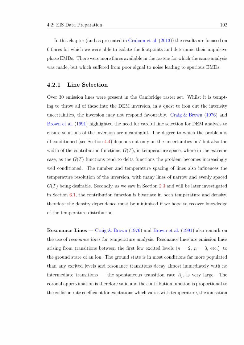
4.2: EIS Data Preparation 102
In this chapter (and as presented in Graham et al. (2013)) the results are focused on
6 flares for which we were able to isolate the footpoints and determine their impulsive
phase EMDs. There were more flares available in the rasters for which the same analysis
was made, but which suffered from poor signal to noise leading to spurious EMDs.
4.2.1 Line Selection
Over 30 emission lines were present in the Cambridge raster set. Whilst it is tempt-
ing to throw all of these into the DEM inversion, in a quest to iron out the intensity
uncertainties, the inversion may not respond favourably. Craig & Brown (1976) and
Brown et al. (1991) highlighted the need for careful line selection for DEM analysis to
ensure solutions of the inversion are meaningful. The degree to which the problem is
ill-conditioned (see Section 4.4) depends not only on the uncertainties in I but also the
width of the contribution functions, G(T ), in temperature space, where in the extreme
case, as the G(T ) functions tend to delta functions the problem becomes increasingly
well conditioned. The number and temperature spacing of lines also influences the
temperature resolution of the inversion, with many lines of narrow and evenly spaced
G(T ) being desirable. Secondly, as we saw in Section 2.3 and will be later investigated
in Section 6.1, the contribution function is bivariate in both temperature and density,
therefore the density dependence must be minimised if we hope to recover knowledge
of the temperature distribution.
Resonance Lines — Craig & Brown (1976) and Brown et al. (1991) also remark on
the use of resonance lines for temperature analysis. Resonance lines are emission lines
arising from transitions between the first few excited levels (n = 2, n = 3, etc.) to
the ground state of an ion. The ground state is in most conditions far more populated
than any excited levels and resonance transitions decay almost immediately with no
intermediate transitions — the spontaneous transition rate Aji is very large. The
coronal approximation is therefore valid and the contribution function is proportional to
the collision rate coefficient for excitations which varies with temperature, the ionisation

4.2: EIS Data Preparation 103
abundance — also a steep function of only temperature — and a number of constants.
Electron density does not influence any of these parameters strongly. Of course, in the
full calculation for the relative level population of the ground state, transitions to other
levels are included which may have a density dependence of their own, however the
reduction in population of the ground state is minimal and the coronal approximation
will still hold.
Another attribute of these lines is their very high transition probabilities (also
known as the oscillator strength, see Section 5.5.4) meaning that they easily absorb
and re-emit photons of equal energy to the transition energy. The re-emitted radiation
is known as resonance radiation and was discovered by Robert Wood whilst studying
Sodium vapour (Wood 1905). For use in DEM(T) analysis this quality can make them
much brighter, reducing measurement uncertainties. The resonant behaviour varies
from ion to ion and at the time of writing Graham et al. (2013) we did not have access
to enough information to base the line choice entirely on such lines though a selection
of resonance lines are tabulated in Pottasch (1964). Also, the limited selection of lines
available did not afford us the luxury of picking only resonance lines. However, without
fully understanding the emission and re-emission characteristics, difficulties may arise
in estimating the optical depth of resonance lines in the transition region. We discuss
this further in Chapter 5 but mention here that the high oscillator strength makes
them very susceptible to absorption and scattering (Andretta & Jones 1997). We feel
it was important to note these effects for future analysis and EIS study design since it
has not been explicitly mentioned in many recent DEM analyses.
Density Sensitivity — In spite of this we can still check the temperature and density
sensitivity of the available lines before selecting them. Of the lines present in these
rasters we have narrowed the selection down to 15 which cover the temperature range
log T = 5.0 − 8.0. Heavily blended lines or those with high optical depths (e.g. He-
lium II) have also been ignored. Details of the lines are found in Table 4.1. Figure
4.1 shows the G(T ) functions calculated for an electron density of 1011 cm−3, coro-
nal abundances (Feldman et al. 1992) and CHIANTI’s own ionisation equilibrium file

4.2: EIS Data Preparation 104
(Landi et al. 2012). The reasoning behind these choices is left to Section 4.4.1.
The peak temperature contributions are spread evenly across the range up to
log T = 7.0 where the high temperature lines start to tail off. In most lines ∼ 90% of
the function is contained within log∆T ∼ 0.5, bearing in mind that the plot is log-
arithmic so the contributions functions in Figure 4.1 appear far more sharply defined
on a standard scale. Some lines are not ideal but are the only choice to cover certain
temperatures. The high ionisation energy of He-like O vii leads to enhanced recom-
bination at high temperatures back into O vi (Mariska 1992). The O vi contribution
function therefore has an elongated high temperature tail, yet most of contribution
here should be sufficiently small compared to the peak. The resonance Fe xv 248A
line is also very broad but is well observed in EIS.
The density sensitivity of a line’s contribution function is shown by plotting them
at the line’s peaks formation temperature against density. It is clear from Figure 4.2
that G(Tmax, n) for most lines varies by less than 25% for transition region densities of
log ne = 10.0 − 14.0. In the iron G(n) functions, left hand figure, Fe xiii and Fe xiv
rise at densities below log ne = 10.0. These are not the density sensitive transition
of the diagnostic pair used in Chapter 3 but some dependence on density will arise
as some of the level population migrates to the metastable levels. However, footpoint
densities observed in these lines are on the order of at least 1010 cm−3 so this should
not concern us. The reasoning is the same for O v, although its G(n) flattens above
1012 cm−3. In Graham et al. (2013) these lines were part of the EMD, but subsequent
research on diagnostics at the formation temperature of O v ( logT = 5.4) in Chapter
5 suggests that the footpoint density may be higher than the logne = 11 set here. It
may be sensible in future to set the DEM contributions at a constant log ne = 12 to
minimise uncertainty here, or indeed adjust the line selection.
Intensities — As mentioned earlier, data uncertainties inherently lead to non-unique
EMD solutions being returned by inversion methods. To minimise this we require
careful measurement of the integrated line intensity, therefore for lines blended with
multiple temperature components, contributions must be carefully removed from the

4.2: EIS Data Preparation 105
Table 4.1: Emission lines selected for EMD analysis with rest wavelengths and
peak formation temperatures.
Ion λ (A) log10T (K)
O v 248.460 5.4
O vi 184.118 5.5
Fe viii 185.213 5.7
Mg vi 268.991 5.7
Si vii 275.361 5.8
Fe x 184.537 6.1
Fe xi 188.216 6.2
Fe xii 195.119 6.2
Fe xiii 202.044 6.3
Fe xiv 274.204 6.3
Fe xv 284.163 6.4
Fe xvi 262.976 6.4
Ca xvii 192.853 6.8
Fe xxiii 263.766 7.2
Fe xxiv 192.028 7.2
line in question — see Section 4.2.3. Lines harbouring large undocumented blends, or
those which are blended with multiple lines of similar intensity and centroid position
are ignored.
If for example a pair of lines at similar temperatures are present within one profile,
the sum may be used in conjunction with the total of both contribution functions, but
this situation is not common within the EIS spectrum. An extension of this analysis
is useful for spectrometers with low spectral resolution such as the EUV Variabil-
ity Experiment (EVE) (Woods et al. 2012) on board the Solar Dynamics Observatory
(SDO) (Pesnell et al. 2012), and in Chamberlin et al. (2012) multiple lines at similar
4.2: EIS Data Preparation 106
5.0 5.5 6.0 6.5 7.0 7.5 8.0log10 T [K]
10−28
10−27
10−26
10−25
10−24
10−23
Tem
pera
ture
Res
pons
e
O V
O VI
Fe VIII
Mg
VISi VII Fe
XFe
XIFe XII
Fe XIII
Fe XIV
Fe XV
Fe XVI
Fe XVII
Ca XVII
Fe XXIII
Fe XXIV
Figure 4.1: Contribution functions G(T ) for emission lines calculated with
coronal abundances, CHIANTI’s own ionisation equilibrium file, and a constant
density of 1011cm−3
temperatures were grouped together into a single averaged intensity measurement. In
principle this could be used in our DEM analysis to minimise measurement uncertain-
ties but with the limited line selection available in EIS this is not feasible for many
temperatures.
4.2.2 Line Flux
Data for the chosen lines were once again calibrated and fitted using the standard
eis prep and eis auto fit SolarSoft routines as discussed in Chapter 3 Section 3.2.1.
An exception is the analysis of Ca xvii which uses a method described in more detail
in 5.2. We also use the same correlation method in 3.2.2 to correct a measured 17′′
North-South and 1′′ East-West offset between the two separate wavelength bands on
the instrument’s CCD. As discussed in the following, only one raster was used in
each event so there was no need to correct for any temporal effects like pointing drift.
Uncertainties in the line intensities were also found as in 3.2.1.
We extracted for each emission line the fitted integrated line intensity averaged over
a 2′′ × 3′′ area around a footpoint (1× 3 pixels). In the previous chapter we found that

4.2: EIS Data Preparation 107
Figure 4.2: Peak contribution functions for EMD lines as a function of density.
Temperature is held constant at the contribution function peak Tmax and coronal
abundances with CHIANTI’s own ionisation equilibrium file are used for the
calculation.
the impulsive brightenings seen in EIS are on the order of 1-2′′ and the same is true
in the events used here. The strongest footpoint emission is mostly contained within
one slit position 2′′ wide in the x direction and 2-3′′ in the y. We have averaged the
centre pixel with those above and below to match the slit width and improve the signal
to noise ratio. To equally bin in the x-direction would sample 6′′, gathering too much
of the surrounding area. Our binning accounts for the spatial extent of the footpoint
and again covers some of the uncertainty in correlating between the long and short
wavelength CCDs.
The choice of centre footpoint point pixel was made using the brightest pixel in the
cool Fe viii raster. In the previous chapter we found low temperature lines brighten
quickly and are a good indicator of the low atmosphere response to flare energy de-
position (Fisher et al. 1985). While He ii is thought to radiate extremely well during

4.2: EIS Data Preparation 108
impulsive heating (Allred et al. 2005), it has a number of higher temperature blends so
Fe viii chosen as an alternative bright transition region line. More recent work has also
begun to shed light on the early temporal evolution of impulsive phase footpoints, es-
pecially since the advent of high cadence instruments on board SDO (Chamberlin et al.
2012; Qiu et al. 2013).
At the time we decided not to subtract a pre-flare background from the footpoint
emission. The reasoning was that it allowed us to make consistent comparisons with
the EMDs from historical observations, which did not make a subtraction either, and
with the theoretical work discussed in Section 4.6; which treats emission from the entire
emitting column, not only the flare excess. Yet it does remain a point of interest, as
the shifted evaporating components of the lines may show a different distribution to
any stationary one. A brief discussion on this is given later.
4.2.3 Line Blending
Even after careful selection, a number of transitions contained unavoidable blends that
needed removal. In blended lines the true intensity can be often recovered very suc-
cessfully using various fitting techniques and other observed lines within the raster
set. The CHIANTI v7.0 atomic database Dere et al. (1997); Landi et al. (2012) was
used to identify lines contributing to the measured line profiles. Synthetic spectra
are created for a variety of DEMs. CHIANTI does this by calculating I for all lines
within a wavelength range using the G(T ) functions, a prescribed DEM, abundances
and density. Here we use the same density and abundances as before, but check the
predicted intensities using both the CHIANTI flare Dere & Cook (1979) and active
region DEMs Vernazza & Reeves (1978). While this method is not perfect, it does
assume we have some knowledge of the plasma to begin with, it will highlight the more
significant blends. We now discuss the significant blends in our line selection.
O v — The 248.460A line has a small blend of Al viii at 248.459A which is predicted
to be less than 10% during flare conditions. It is too small to accurately remove by

4.2: EIS Data Preparation 109
fitting but we estimate it should not be significant during flares. A blend in the blue
wing is also seen in the footpoints and is removed using a second Gaussian component
— Section 5.2 has more details on these blends.
Fe viii — Two predicted blends of Ni xxiv 185.166 and Ni xvi 185.230 are present in
the low temperature Fe viii 185.213 line. A triple Gaussian fit finds these effectively
and revealed very small contributions of Ni xvi 185.230 in the footpoints, around 8%
of the Fe viii intensity, and a negligible amount anywhere else. In some footpoints the
red wing Ni xvi 185.230 was stronger than the almost negligible intensity predicted
by CHIANTI flare DEM — as much as 17% in one footpoint. Interestingly, in some
events a very large contribution was found in regions 2-3′′ away from the footpoint.
This is puzzling as the line has a formation temperature of 107.2 K. It is possible that
the line is misidentified in CHIANTI, or perhaps is a highly red-shifted component of
the Fe viii line. Either way it far enough away from the footpoints to not be a concern
for our EMD.
Fe xxiv — Care must be taken to extract Fe xxiv 192.028 as even though it normally
dominates in flare loop conditions, the nearby transition region lines of Fe viii 192.004
and Fe xi 192.021 are bright in the active region. This work concentrates on an earlier
phase in the flare where the Fe xxiv emission may be much fainter, therefore these
blends must be removed. While they are too close in wavelength to accurately fit
Del Zanna et al. (2011) described a method to remove them using intensity ratios to
other lines. The target Fe xi 192.021 line forms a known intensity ratio with an other
observed Fe xi line at 201.734A. The measured λ201 intensity can then be used to
estimate the λ192 intensity in the footpoint. We find the ratio of 192.021/201.734
intensities in background moss/active regions to be 0.43 compared to the CHIANTI
value of 0.6. This difference is possibly due to some Fe xii emission within the 201A
line that decreases the flux ratio. We have therefore used the predicted ratio of 0.6 to
remove the 201A blend, as in this case we are less likely to over estimate the Fe xxiv
intensity.

4.3: Flare Observations and Footpoint Selection 110
The Fe viii 192.004 intensity is predicted by CHIANTI to be around 10% of the
Fe xi line and is almost negligible. The referee for the published paper on this work
suggested the lower temperature lines such as Fe viii may be preferentially enhanced
during the impulsive phase and contribute more to the blend than Fe xi. While a
sound suggestion we see no evidence for this as enhanced emission is found in lines
extending to all temperatures. In most of the events the rasters are also sampled some
way into the impulsive phase and high temperatures plasma will have had time to form.
Accounting for these contributions removes the majority of the active-region emission
from the Fe xxiv raster (seen in Figure 4.4). If we look at the corrected average mean
background level, in areas away from the footpoint, the level is now lower than the un-
certainty for the bright footpoint. We are therefore confident the remaining intensity
is from Fe xxiv alone.
Ca xvii — The Ca xvii 192.853 line is found in a complex grouping of six O v and
two Fe xi lines. The extraction of this challenging but is well documented (Ko et al.
2009; O’Dwyer et al. 2010; Del Zanna et al. 2011). We have adopted the approach
in Ko et al. (2009) but as one of the O v lines forms a density diagnostic we have
explained it in far more detail in Section 5.2.
4.3 Flare Observations and Footpoint Selection
The Cambridge rasters were run during a period of mild solar activity towards the end
of the last solar cycle. For durations of 1-3 hours the study was run while centred on a
flaring active region. The rasters were repeated in continuous sequence and caught six
small flares with compact footpoints fitting our requirements. The flares range from
B1.8 to C1.1 in GOES energies and are identified in Table 4.2 with the GOES 1-8A
light curves plotted in Figure 4.3.
The light curves for these events are highly impulsive. In most events the rise phase
is completed within 4-5 minutes with the slowest peaking in just under 10 minutes.
While a steep SXR curve can be a good indication of strong footpoint emission, it

4.3: Flare Observations and Footpoint Selection 111
does mean that the 3 min 52 sec raster cadence is only capable of taking one or two
snapshots of the impulsive footpoints, and unlike the previous chapter not much can
be learned about the temporal evolution from the EUV rasters.
Ideally RHESSI HXR imaging and spectroscopy would be used to verify that the
EUV enhancement corresponds to the HXR energy deposition site. However, RHESSI
HXR data were not consistently available in all events. As a substitute, the time
derivative of the GOES SXR emission can be used as a proxy for the HXR emission.
Following the work by Neupert (1968) (see the discussion in Section 1.3) we now find
that in a high proportion of flares the rate of change of the SXR emission follows the
HXR light curve. Assuming this, we have systematically used the GOES derivative to
find the time of maximum energy deposition; a dashed line on the light curves in Figure
4.3 marks the peaks and was used as a guide to select the EIS raster corresponding to
the impulsive phase peak. In most events this was academic as the entire impulsive
phase was contained within the raster limits shown by the dotted lines. For Event (d)
we found the SXR derivative was close to the SXR peak and the raster represents both
peaks. In Event (c) while the derivative peaked early during the SXR rise, the peak
was very close to the end of the early raster, as little EUV enhancement was found in
footpoint for this raster we have chosen the later one.
We must also note that each x position within the raster represents a 10 second
time interval and the flare evolves as the slit position scans West to East. For the
footpoints discussed below, the time at which the slit crosses the footpoint is marked
by a diamond on the light curve. In Event (a) the observed footpoint position is slightly
ahead of the SXR derivative peak, Events (d) and (e) occur roughly near the SXR peak,
and by chance the footpoint position in Event (b) fell precisely at the derivative peak!
The selected rasters are shown in Figure 4.4 for the Fe viii and Fe xxiv lines,
illustrating the flare appearance at 500,000 K and 16 MK. In all events bright emission
has risen dramatically in both lines and is found at the same location. Fe viii tends
to appear more compact and Fe xxiv, while rooted in the same spot, extends further
across the region. Event (b) exhibits the classic flare appearance, compact emission at
cool temperatures, while a larger loop structure reaches to the South-East in Fe xxiv.

4.3: Flare Observations and Footpoint Selection 112
(a) (b) (c)
(d) (e) (f)
Figure 4.3: GOES 1-8A light curves of each event. A pair of dotted vertical
lines represent the start and end times of the EIS raster and a single dashed
line marks the GOES derivative maximum for the event. The time at which the
spectrometer slit scans each footpoint is marked with a diamond on the light
curve.
Event (a) is sampled slightly earlier in its impulsive phase and both of its footpoints are
bright, and compact, in both lines. At a later stage Fe xxiv becomes more significant
as evaporating hot material begins to fill loop structures. Other events such as (f)
have more elongated ribbon structures, yet in all events at least a small component of
Fe xxiv emission is found covering the same location as Fe viii. From the earlier work
by Milligan & Dennis (2009) and Graham et al. (2011) we have learned that compact
brightenings in the EUV can be associated with RHESSI HXR observations revealing
the flare energy deposition site. Also, as found in the previous chapter and in Milligan
(2011) enhanced densities have been seen to occur at the location of impulsive-phase
footpoints. In the diagnostics performed in Chapter 5 we will show that this is still the
case for these events. Given this morphology throughout the EIS temperature range

4.4: DEM Technique 113
we are confident in identifying the flare footpoints, as marked with white arrows in
Figure 4.4.
A number of the flares in question have been studied in detail before (but not
for the purpose of finding EMDs) and the findings may help us later. High velocity
evaporation flows were found in Event (b) by Milligan & Dennis (2009) using EIS, and
were found to be co-spatial with EUV enhancements and HXR footpoints imaged by
RHESSI. Milligan (2011) examined the flare further on the subject of non-thermal line
broadening. Event (f) in Del Zanna et al. (2011) exhibited chromospheric evaporation
signatures along with footpoint electron density enhancements. The evaporating com-
ponent of the emission was also suggested to have an iso-thermal emission measure at
∼ 10 MK.
4.4 DEM Technique
As we discussed in Section 2.3 the inversion of Equation 4.1 is an ill-posed problem
given the uncertainties in the line flux and contribution functions. A single solution for
ξ(T ) should exist based on the conditions in the footpoint plasma. However, not only do
uncertainties in the measurements of I lead to a range of non-unique solutions, the un-
certainties in ξ(T ) are amplified by any attempts to directly invert the equation. Over
the years many different methods to find ξ(T ) have been developed each with their own
advantages and disadvantages (Fludra & Sylwester 1986; Monsignori Fossi & Landini
1991).
Forward fitting approaches exist in various forms but most start from a model
or functional form for the DEM. For example Weber et al. (2004) used a series of
spline functions, with Aschwanden & Boerner (2011) forcing a number of iso-thermal
Gaussian profiles. The minimisation is straightforward to perform but the results can
only verify how well a single model represents the data. H. Hudson & P. Chamberlin are
developing a technique of fitting the entire SDO/EVE spectrum and minimising a DEM
based on the synthetic CHIANTI spectrum. While extremely slow computationally it
will remove the need for any model, although it is still at the whim of uncertainties in

4.4: DEM Technique 114
(a) (b) (c)
(d) (e) (f)
Figure 4.4: EIS rasters for each event in Fe viii at 500,000K and Fe xxiv at
16 MK showing the morphology at low and high temperatures. A white arrow
marks the footpoint positions chosen for EMD analysis in each raster. Black
arrows in panel (b) also highlight the regions used in determining a loop top and
active region EMD (see Section 4.6).
-
the atomic data. Markov chain Monte Carlo (MCMC) approaches also do not require
any a priori model (Kashyap & Drake (1998) from the PINTofALE software library)
but are again very slow and occasionally prone to finding un-physical temperature
components if not used with care (Hannah & Kontar 2012).
The technique we have used to invert Equation 4.1 was developed by Hannah & Kontar
(2012) based on the inversion of RHESSI photon spectra in recovering the electron en-
ergy distribution (this is explained fully in Kontar et al. (2004)). The Hannah & Kontar
4.4: DEM Technique 115
(2012) inversion (HK) used here has the advantage of requiring no a priori knowledge
of the expected DEM form, and errors in both the temperature and emission measure
domain can be found. While not a major concern for a small number of events, the
technique is computationally fast.
Hannah & Kontar (2012) compared the new technique to other more established
MCMC methods using both simulated and observed data. The results are indeed
favourable for the regularized method which is capable of robustly returning the DEM
in a wide variety of cases. Recently more authors have begun to make use of the high
speed inversion (Battaglia & Kontar (2012), Fletcher et al. (2013), Hannah & Kontar
(2013)), finding it especially suited to producing large sets of time-dependent DEMs
with data from SDO’s Atmospheric Imaging Assembly (Lemen et al. 2012). Here, we
supply the reader with enough background to understand the meaning of the inputs
and generation of errors in the method, based on what is shown in Kontar et al. (2004)
& Hannah & Kontar (2012), but refer them to the references for a more complete
explanation and derivation of the solutions used.
For a discrete number of observable line fluxes, Ii, the original problem to invert
Equation 4.1 must be written as a system of linear equations. The integral equation
can be rewritten in the form
Ii =N∑j=1
Ki,jξ(Tj) (4.16)
where Ki,j is a matrix of the i contribution functions over a discrete temperature
range of j intervals, and ξ(Tj) is the DEM defined over the same range and assumed
to be constant within each temperature interval. We therefore aim to solve the system
of linear equations given in matrix form by
Ii = Ki,jξ(Tj). (4.17)
Essentially the problem becomes a minimisation of
∣∣∣∣∣∣∣∣Kξ(T )− I
δI
∣∣∣∣∣∣∣∣2 = min (4.18)

4.4: DEM Technique 116
to find the best fit ξ(T ) where ||x||2 is the Euclidean norm defined by∑N
j=1 x2i .
When uncertainties are present in both I and K, solutions to this quickly amplify the
uncertainties and introduce non-physical oscillatory components. In order to avoid
these unrealistic solutions, Tikhonov (1963) showed that such integral inversions can
be performed using constraints requiring that the inverted solution, ξ(T ), must be
subject to some conservation law or have a continuous form for example. The addition
of constraints to help better condition the problem is known as Tikhonov regularization.
Using Lagrangian multipliers the problem can be rewritten as
||Kξ(T )− I||2 + λ ||L(ξ(T )− ξ0(T ))||2 = min . (4.19)
where is λ regularization parameter, L is the constraint matrix, and ξ0(T ) an initial
guess solution. The constraints can take many forms depending on the problem at
hand. Where L = 1, i.e the identity matrix, the regularization is said to be of zero-
order. In our case a zero-order constraint means the integral of the inverted DEM in
temperature must be less than the total emission measure in all observed lines. Simply,
the total number of electrons predicted can not be greater than the total number
observed. In all the DEM inversions used here we make the restriction that the DEM
solution must be differentiable, ensuring it is a smooth and not discontinuous function,
which is reasonable if the temperature distribution can be described by a differential
equation as in Section 4.1.2. To achieve this first-order regularization L becomes a
differentiation operator (Kontar et al. 2004). We should note, however, that this may
be a strong assumption in certain cases. The DEM of a loop in conductive equilibrium
theoretically has a discontinuous, high temperature cut-off. Steep high temperature
loop components were also thought to be observed in the EMDs of Widing & Hiei
(1984) that merge with the shallow footpoint component. However, our improved
spatial resolution will ensure such blending of EMDs is minimal.
Attempts to solve Equation 4.19 are computationally intensive. General Singular
Value Decomposition (GSVD) Hansen (1992) can be used to find a solution giving
ξλ(T ) which depends on the regularization parameter λ. Not only is this approach

4.4: DEM Technique 117
faster computationally, it can also help suppress unwanted oscillatory solutions.
The choice of regularization parameter is not uncovered through the solution how-
ever, and is left to either foresight of the problem or trial and error. A value for λ,
which gives the full solution ξλ(T ), can be found based on the expected residuals of
the data. By forming the minimisation
1
N
∣∣∣∣∣∣∣∣Kξλ(T )− I
δI
∣∣∣∣∣∣∣∣2 = α , (4.20)
known as Morozov’s discrepancy principle (Morozov 1963), and by iterating the
method one finds the value for λ, therefore ξλ(T ), that meets the requirement α.
The value α is the regularization tweak parameter which controls the expected degree
to which the residuals between the observed intensities and intensities predicted by
ξλ(T ) are distributed — in essence it sets the χ2 required of the fit. Lower values of
α place more emphasis on the data and regularization will be strongly bounded by
the observations. On the other hand, higher values leave the regularization with more
freedom, which can help for poorly sampled data, but the solution may start to resemble
the constraints as opposed to the actual plasma distribution. In our DEMs the effects
of this over-regularization are clearly seen in DEM errors and we find that α = 2 − 3
returns a solution that has no oscillatory components yet is not over-regularised (see
Figure reffig:alpha). A final constraint we make is to ensure that the DEM solution is
positive for all temperatures by choosing the regularization parameter that minimises
Equation 4.20 while maintaining ξλ(T ) > 0
An initial guess solution ξ0(T ) can be obtained by taking the emission measure
given for an isothermal plasma in each contribution function. The isothermal solutions
represent the maximum emission possible at each temperature given by Ii/G(Tj); also
known as EM-Loci curves, they are used here as a physically realistic place to start the
minimisation.
Turning to the errors in the DEM solution, the HK method returns both an un-
certainty δξ(T ), and temperature resolution δT at each point in the DEM solution.
We will not delve into much detail as their origin is not essential to understanding the

4.4: DEM Technique 118
(a)5.5 6.0 6.5 7.0 7.5
log10 Temperature [K]
1026
1027
1028
1029
1030
Em
issi
on M
easu
re [c
m−
5 ]
14Dec07 (01:37:24)
(b)5.5 6.0 6.5 7.0 7.5
log10 Temperature [K]
1026
1027
1028
1029
1030
Em
issi
on M
easu
re [c
m−
5 ]
14Dec07 (01:37:24)
Figure 4.5: Example EMDs using a regularization tweak parameter of α = 1.0
(left) and α = 5.0 (right).
-
solutions (it is well covered in Hannah & Kontar (2012)), but note that they tell us
about both the limitations of our data, and when the solution is over-regularised.
Figure 4.5 shows two test EMDs derived from data for the HK technique. The
EM-Loci curves are displayed in coloured lines bounding the EMD shown in black.
The grey shaded error represents the extent of the errors in both EM and temperature
space, a solution can therefore be found anywhere in this region. The EMD in the
left hand figure, for α = 1.0, is strongly constrained by the minimum EM-Loci curves
and the data in places, yet displays the oscillatory behaviour of an under regularized
solution, i.e the two sharp dips with large errors in the middle of the temperature range.
In the right hand figure a large α of 5.0 is used and the effects of an over-regularised
solution are apparent. The temperature uncertainties are ballooned and therefore any
temperature resolution is lost. In our fitting we aim to choose α to ensure that our
solution sits somewhere between these two extremes.
4.4.1 DEM Inputs and Uncertainties
Now that we have decided on a suitable set of lines and G(T ) functions, obtained the
footpoint line intensities and uncertainties, we are in a position to perform the inversion

4.4: DEM Technique 119
to find ξ(T ). One final point is that the G(T ) functions are not completely accurate and
have an inherent uncertainty themselves arising from errors in the calculation of cross
sections, transition rates etc. In a private communication with P. Young, a founding
member of the CHIANTI team, a systematic error 20% was agreed to account for the
total calibration uncertainty between lines. The error is added to the existing flux
errors for the inversion.
The contribution functions were seen in Section 4.2.1 where coronal abundances,
the CHIANTI ionisation equilibrium file, and a constant density of 1011cm−3 were used
in their calculation. The value of electron density was chosen based on the footpoint ob-
servations (see e.g. Watanabe et al. 2010; Graham et al. 2011; Milligan 2011). While
the atmosphere is unlikely to be homogeneous in density, the contribution functions
are not strongly affected by density variations as the density-sensitive lines have been
removed from the analysis. The choice of density is therefore not critical.
Elemental abundances relative to hydrogen however may bias the shape of an EMD.
Low first ionisation potential (FIP) elements are found to be enhanced in coronal
material compared to the photosphere while high FIP elements are unchanged. In the
standard flare model, material in the footpoints is brought to coronal temperatures and
rises into loops through evaporation. The chromospheric, possibly part photospheric
material, then mixes with plasma in the corona. The abundances will therefore depend
on the relative amount of footpoint to coronal material within the loop. In the footpoint
it is likely a similar picture, as downward moving plasma can move material from its
favoured quiescent height. In terms of flare spectra, the choice of abundances is not
straightforward (Athay 1994; Feldman et al. 2004). Only O v and O vi in our analysis
are high FIP and should be relatively insensitive to the abundances. For elements
like iron that are low FIP, the abundances can change by a factor of 4 between the
photosphere and corona. We have picked coronal abundances to start with but we will
investigate the effects of varying the abundances fully later in Section 4.5.4.
The ionisation equilibrium files set the abundances of each ion relative to its parent
element. They differ slightly based on how they are determined and the experimental
data used, therefore the choice is similarly uncertain. We test this later but use the

4.5: Flare EMDs 120
default CHIANTI set for now.
4.5 Flare EMDs
The EMD derived from EIS data for the six events are presented in Figure 4.6. The
inverted ξ(T ) solutions have been converted to emission measure units of cm−5 by
integrating over the temperature spacing ∆T = 1.14 as shown in Section 4.1.1 — the
errors are converted likewise. The best fit solutions for the EMD are shown in black
lines and are bounded by the inversion errors in a grey shaded area. The area represents
the extent of both errors in EMD(T) and in log T space, therefore the solution may lie
anywhere within these bounds. The regularized solutions for all events remain within
the bounds of the coloured EM-Loci curves confirming that they fall below the expected
maximum total emission.
For each EMD the regularization tweak parameter α was adjusted by hand through
integer values to achieve the best solution. To recall, this sets the expected χ2 value
for the inversion to target with a lower α placing more weight on the data. To gain
the most physical information from the inversion we try to set this as low as possible
without creating spurious inversions. The solutions were relatively insensitive to α
between the limits of over and under-regularisation so no further iterative method was
required.
The data in Events (a) and (d) seemed to invert very well and the EM was mostly
within ±100.15 cm−5. Event (f) proved tricky to balance being over regularized and
returning a stable solution. The highest χ2 that gave a smooth solution quickly gave rise
to very broad temperature errors. We put this down to perhaps line blending given the
complicated ribbon morphology in this event. If this is true it is interesting to find the
inversion has some inherent capability in identifying bad data. At temperatures above
107 K the solutions all appear to fall off in EM expectedly and have no anomalous high
temperature components, although the temperature resolution above 107 K is poor due
to the broad G(T ) response in Fe xxiii and Fe xxiv so the exact cut off is uncertain.
This lack of constraint makes it impossible to make physical conclusions beyond these

4.5: Flare EMDs 121
(a)5.5 6.0 6.5 7.0 7.5
log10 Temperature [K]
1026
1027
1028
1029
1030
Em
issi
on M
easu
re [c
m−
5 ]
14Dec07 (01:37:24)
χ2 = 1.9 (b)5.5 6.0 6.5 7.0 7.5
log10 Temperature [K]
1026
1027
1028
1029
1030
Em
issi
on M
easu
re [c
m−
5 ]
14Dec07 (01:37:24)
χ2 = 3.0
(c)5.5 6.0 6.5 7.0 7.5
log10 Temperature [K]
1026
1027
1028
1029
1030
Em
issi
on M
easu
re [c
m−
5 ]
14Dec07 (01:37:24)
χ2 = 2.6 (d)5.5 6.0 6.5 7.0 7.5
log10 Temperature [K]
1026
1027
1028
1029
1030
Em
issi
on M
easu
re [c
m−
5 ]
14Dec07 (01:37:24)
χ2 = 2.0
(e)5.5 6.0 6.5 7.0 7.5
log10 Temperature [K]
1026
1027
1028
1029
1030
Em
issi
on M
easu
re [c
m−
5 ]
16Dec07 (01:37:24)
χ2 = 3.5 (f)5.5 6.0 6.5 7.0 7.5
log10 Temperature [K]
1026
1027
1028
1029
1030
Em
issi
on M
easu
re [c
m−
5 ]
22May07 (01:37:24)
χ2 = 3.0
Figure 4.6: EMDs shown in black for each event in emission measure units
cm−5 and the uncertainty limits of the solution by a shaded grey area. The
coloured curves show measured line intensity divided by the contribution function
indicating the maximum possible emission, i.e. the EM loci curves.
temperatures. Unsaturated, soft X-Ray observations from Hinode/XRT could have
helped but were unavailable for all flares.

4.5: Flare EMDs 122
4.5.1 Measured Footpoint EMD Profiles
While performing the EMD inversion the first striking point was the similarity of the
EMD profiles and consistency of what appeared to be an almost constant gradient.
Naturally, this led to a literature check on EMD gradients and formed the direction of
this chapter. In the footpoint EMDs above they share a similar profile; increasing with
an almost constant gradient of EM(T ) ∼ T to a peak around log T = 6.9 and falling off
quickly at higher temperatures. However, a closer look shows that there are deviations
from a constant slope and variations between the events. The bumpy appearance of
the EMD in Events (a), (b), and (f) is most likely a result of uncertainties in either the
intensities or atomic data, as the undulations are of a comparable size to the width of
the shaded error region. Event (e) is perhaps the best example of a constant gradient
as the EMD is very well constrained.
Looking at the profiles, we can roughly estimate the gradient up to the peak by
taking a line between two end points at log T = 5.5 − 6.9. We start from log T = 5.5
on the basis it is far enough in to avoid the badly constrained edges. An estimate
of the spread of possible gradients is made by taking the maximum and minimum
of the EM error boundary at the low temperature end, and finding the slope to the
opposite bounds at the high temperature end. For Event (b) we measure a slope of
EM(T ) ∼ T 0.95±0.27, very close to the logEM ∝ T expected for a conduction-balanced
atmosphere. For all of the events the gradients do not vary significantly and a gradient
of 1 is certainly possible within the error ranges shown in Table 4.2.
A discontinuity at high temperatures like that observed in Widing & Hiei (1984)
is not seen in any event. However, there is evidence to suggest a marginal break
at log T = 5.7 in the Events (a), (b), and (c), where the EMD flattens at very low
temperatures. Taking the gradient in Event (b) from log T = 5.7 − 6.9 returns a
steeper gradient of 1.04±0.45; as this event is the earliest sampled it may hint that the
conduction/radiation balanced part of the atmosphere extends to lower temperatures
as the heating continues, though we reinforce that the evidence could be marginal given
the uncertainties in the inversion. On the other hand the break in Event (c) is certainly

4.5: Flare EMDs 123
significant compared to the size of the shaded error region.
Peak emission measures occur at log T = 6.9 and vary between 1028 and 1029 cm−5
and do not appear to be strongly correlated to the GOES class, perhaps expected for
a small selection of low energy events not sampled at consistent times (these values
are tabulated alongside the gradients in Table 4.2). The emission measure in all events
falls off quickly above log T = 6.9 suggesting that this may be a limit to the maximum
footpoint temperature observed, although we do not have any higher temperature data
to confirm this. However, if we look at the radiative loss curve (as seen in Figure 1.4),
we see that radiative losses from plasma above log T = 6.9 also fall off rapidly by
a factor of around 8 to a minimum at log T = 7.2. It may be expected then that
as the flare energy input increases (moving from GOES C class to M or X) the peak
temperature of the EMD remains unchanged, as higher temperatures will contribute
less to the distribution. Free-free emission above log T = 7.0 may still of course be
observed by XRT or RHESSI.
If the total flux from non-thermal electrons was to rise then the overall emission
measure would be expected to rise across the temperature range. More importantly,
the shape of the EMD in temperature may depend on the spectral index and low energy
cut-off of the HXR spectra. In a collisional thick-target model higher or lower energy
electrons will penetrate to different depths, heating different layers of the atmosphere.
For example a relatively soft spectrum, as seen in Chapter 3, could deposit energy
higher in the atmosphere where it is easier to heat. If the EMD is sensitive to these
parameters then a study using a wide range of flare energies and HXR coverage could
be used to confirm such a model. Creating synthetic EMDs using a range of beam
parameters from a model such as Allred et al. (2005) would be an ideal starting point
to investigate this.
4.5.2 EMDs for Different Solar Plasmas
Consistent flare EMDs are desirable but on the other hand the inversion method is
subtle, and in principle could influence the results. We can verify that the similarity

4.5: Flare EMDs 124
Table 4.2: Event EMD parameters sorted by GOES Class. The gradient is
calculated between temperatures of log T = 5.5− 6.9.
Flare ID GOES Class Event Peak Temp Peak EM Gradient
log10 T (K) ×1028cm−5
SOL2007-12-16T06:22:40 B1.8 (e) 6.9 4.0 1.00 ± 0.21
SOL2007-05-22T23:25:50 B2.7 (f) 6.9 1.0 0.87 ± 0.23
SOL2007-12-14T15:22:00 B8.8 (c) 6.9 8.0 1.38 ± 0.28
SOL2007-12-14T15:54:15 B8.8 (d) 6.9 2.0 0.84 ± 0.28
SOL2007-12-14T01:39:20 B9.6 (a) 6.9 2.0 0.82 ± 0.37
SOL2007-12-14T14:16:30 C1.1 (b) 6.9 6.0 0.95 ± 0.27
of the EMDs determined for different events is not an artefact of the regularization by
testing it with the line fluxes from active region (AR) and flare loop top (LT) plasma.
Event (b) displayed a classic high temperature loop and the brightest pixel in Fe xxiv
was picked for the EMD. A non-flaring region bright in Fe xii was selected in the active
region background to represent the AR EMD; these locations are marked for reference
by black arrows on the second panel of Figure 4.4.
The footpoint EMD is plotted in Figure 4.7 inside a green error boundary and
EMDs for the AR and LT regions are found in orange and blue regions respectively.
EMDs extracted from the AR and LT are indeed different from that of the footpoint,
confirming that the regularization method is responsive to the different plasma dis-
tributions. Noticeable features are the matching EMD gradients of the AR and LT
between log T = 5.8 − 6.3, beyond which the AR plateaus and quickly falls off above
log T = 6.8 while the LT keeps rising, at a gradient close the footpoint, up to a peak
of log T = 7.1. We note that both rise with a slope steeper than EM(T ) ∼ T32 , a
commonly observed gradient for the transition region and low corona (Jordan 1980);
this is plotted for reference in a dashed line.
The referee for Graham et al. (2013) had some invaluable insight which helped

4.5: Flare EMDs 125
further understand the relationship between these EMDs if we consider the AR EMD
to be a pre-flare situation. Emission in the footpoint between temperatures of log T =
5.2 − 6.2 was seen to be greater than in the AR by up to an order of magnitude. As
we suspect from a conventional understanding of flares, this enhancement is likely to
be chromospheric plasma in the process of being heated to flare temperatures. The
point at log T = 6.2 − 6.3 where all 3 EMDs meet is intriguing. While the matching
absolute EM may be coincidental, the break in similarity between AR and LT EMDs
gradients here may indicate that only plasma above log T = 6.2 will make it into the
loop as there is no enhancement at temperatures below this. The flow measurements
in Milligan & Dennis (2009) agrees with the picture, as plasma above log T = 6.2 is
blue-shifted (upflowing) and plasma below this temperature is red-shifted. Analysis of
the plasma velocities will be important in future studies, but we found it reassuring to
see that such arguments can be made from the results and that the behaviour of the
EMDs varies in reasonable ways through the event.
5.5 6.0 6.5 7.0 7.5log10 Temperature [K]
1026
1027
1028
1029
1030
Em
issi
on M
easu
re [c
m−
5 ]
EM(T) ~ T3/2 EM(T) ~ T
Foot Point Active Region Loop Top
Figure 4.7: A comparison of footpoint, loop, and active region EMDs in Event
(b). The purpose of this is to check the regularization response to different
temperature distributions. Gradients of EM(T ) ∼ T and EM(T ) ∼ T32 are
added in dashed lines.

4.5: Flare EMDs 126
4.5.3 Examination of the Assumptions Used
When interpreting spectra during flares we must be aware of the built-in assumption
in the atomic physics. The G(T ) functions in CHIANTI are calculated for an optically
thin plasma in a thermal Maxwellian distribution and in ionisation equilibrium. Is
this assumption sensible in an impulsively heated footpoint? Here we have made some
arguments to check, although a full analysis of the assumptions in one flare will be
carried out later in Chapter 5.
Thermal Equilibrium — We know from RHESSI HXR observations that the elec-
tron spectra in the footpoints have an inherently non-Maxwellian component, due to
bremsstrahlung emission from high energy electrons. While these are responsible for
heating the footpoint plasma, their energy content may be small compared to the to-
tal energy of the distribution; see Krucker et al. (2011). Heating in the footpoint is
intense, easily taking plasma from 10, 000 K to over 106 K in a matter of minutes.
If we discount the non-thermal component for now, can the core of the Maxwellian
plasma remain in thermal equilibrium if it is heated so quickly? The electron-electron
collision time-scale gives us a handle on the rate at which temperature changes can be
equilibrated. For an electron density of 1011 cm−3 and temperatures of 105.5 K and
106.9 K the collision times are 3× 10⁻⁵ and 1× 10⁻³ seconds (see Section 5.5.3 ). This
is much faster than the duration of the impulsive phase, which in Event (b) is ∼ 4
minutes, so the plasma should thermalise quickly.
Ionisation Equilibrium — In low density plasmas the temperature may evolve faster
than the ionisation state of the plasma can catch up. For example O v may not com-
pletely ionise into O vi before the temperature has reached the Tmax for O vi. The
ionisation stage therefore does not match the temperature and lags behind. We dis-
cuss this again in more detail in Section 5.5.2 but note here the calculations of non-
equilibrium ionisation (NEI) states by Bradshaw (2009), who finds that at densities of
1010 cm−3 the ion peak formation temperatures can shift by up to log T = 0.3 K, but

4.5: Flare EMDs 127
by ne = 1012 cm−3 the difference is negligible. For our footpoint densities at around
1011 cm−3 ionisation equilibrium could be a safe assumption. Section 5.5.2 investigates
the effect this has on electron density diagnostics, however, it is not clear at this stage
how to implement NEI states into an EMD analysis. If all of the ion peak formation
temperatures move by a similar amount the EMD slope might be preserved but shifted
in temperature. Of course, this is merely an observation and requires further work in
future.
Optical Depth — The data here extend to much lower temperatures than in the
previous chapter and presumably higher densities if we extend the heating to deeper
layers (see Chapter 5 for evidence of this). Line fluxes could be influenced as this means
the atmosphere may not be completely optically thin throughout the whole region in
which the EMD is produced. From the work in Bloomfield et al. (2002) and Milligan
(2011) we found a means to estimate the optical depth for a given emission line. In
Chapter 5 we improve on the brief calculation in Graham et al. (2013), which ignored
the full integral over depth, and found the optical depth for lines emitting through a
VAL-E atmospheric profile.
Here we show the results for lines used in the EMD analysis in Table 4.3 but refer
the reader to Section 5.5.4 for more details. For the standard VAL-E atmosphere it
appears that many of the lines have relatively large optical depths of over log τ = 1,
however, we must remember that the VAL-E atmosphere is not representative of flares
and even when moving into its transition region temperatures are below 1 MK. The
model can be made more representative for our footpoints if we arbitrarily set the
temperature of the entire atmosphere to log T = 6.8, comparable with the maximum
EM from the EMD. We do not suggest that the entire atmosphere is heated to this
temperature, but it serves to calculate a lower limit for τ . The values in the table
now drop below log τ = 0 which is reasonable. As shown later an optical depth of
1 corresponds roughly to a reduction in intensity of 30% which is comparable to our
I + G(T ) errors. In most of the lines log τ is much less than 1.0 so the optically thin
assumption may stand.

4.5: Flare EMDs 128
Two lines do come to our attention though. Fe viii and Fe xv still have optical
depths of τ = 1 at the higher temperature, indicating they may be problematic at lower
temperatures. Fe xv 248A is a known resonance line with a high transition probability
and Fe viii 185A is excited from a line above the ground state and has high relative
population; both of these factors will increase the optical depth of a line. The EMD
analysis can be rerun after removing these lines and can be seen in Figure 4.8. The
overall profile is not significantly altered by this change although the χ2 to achieve a
positive stable solution is now increased in some events due to the reduced constraint.
The break in profile slope at around log T = 5.8 for Events (a) and (c) is perhaps
clearer now but further constraint at these temperatures would be needed to test this
further.
Through these tests we arrived at the conclusion that the plasma state may indeed
be close to the required assumptions and that the EMD is not strongly influenced;
though we have only arrived at the conclusion through some simple analysis. To fully
understand the effects of non-equilibrium and radiative transfer in a flare atmosphere
is a serious undertaking which requires further modelling and tailored observations.
This is beyond the scope of the chapter but should not be ignored in future studies.

4.5: Flare EMDs 129
Table 4.3: Optical depths at line centre calculated at ne = 1011 cm−3 using
the VAL-E atmospheric parameters. Also shown are the optical depths for a
modified VAL-E model, where the temperature is held constant (log T = 6.8)
and is assumed to be fully ionised (ne = nh).
Ion λ (A) log τ0 log τmod
O v 248.460 -4.75 -7.19
O vi 184.118 -4.04 -6.49
Fe viii 185.213 2.35 -0.02
Mg vi 268.991 1.08 -1.28
Si vii 275.361 1.37 -0.99
Fe x 184.537 1.77 -0.60
Fe xi 188.216 1.78 -0.58
Fe xii 195.119 1.92 -0.43
Fe xiii 202.044 0.28 -2.08
Fe xiv 274.204 1.44 -0.91
Fe xv 284.163 2.35 -0.02
Fe xvi 262.976 -5.13 -7.58
Ca xvii 192.853 0.45 -1.92
Fe xxiii 263.766 -0.33 -2.70
Fe xxiv 192.028 1.10 -1.28

4.5: Flare EMDs 130
(a)5.5 6.0 6.5 7.0 7.5
log10 Temperature [K]
1026
1027
1028
1029
1030E
mis
sion
Mea
sure
[cm
−5 ]
14Dec07 (01:37:24)
χ2 = 1.4 (b)5.5 6.0 6.5 7.0 7.5
log10 Temperature [K]
1026
1027
1028
1029
1030
Em
issi
on M
easu
re [c
m−
5 ]
14Dec07 (01:37:24)
χ2 = 3.0
(c)5.5 6.0 6.5 7.0 7.5
log10 Temperature [K]
1026
1027
1028
1029
1030
Em
issi
on M
easu
re [c
m−
5 ]
14Dec07 (01:37:24)
χ2 = 1.8 (d)5.5 6.0 6.5 7.0 7.5
log10 Temperature [K]
1026
1027
1028
1029
1030
Em
issi
on M
easu
re [c
m−
5 ]
14Dec07 (01:37:24)
χ2 = 1.7
(e)5.5 6.0 6.5 7.0 7.5
log10 Temperature [K]
1026
1027
1028
1029
1030
Em
issi
on M
easu
re [c
m−
5 ]
16Dec07 (01:37:24)
χ2 = 3.3 (f)5.5 6.0 6.5 7.0 7.5
log10 Temperature [K]
1026
1027
1028
1029
1030
Em
issi
on M
easu
re [c
m−
5 ]
22May07 (01:37:24)
χ2 = 3.1
Figure 4.8: EMDs shown the same data but removing the Fe viii and Fe xv
lines to check for optical depth effects.

4.5: Flare EMDs 131
4.5.4 Varying the Abundance and Ionisation Equilibrium
The difficulty in choosing the appropriate values of elemental abundances in the foot-
point plasma was discussed in Section 4.4.1. It was also not clear which set of ionisation
equilibrium files should be used. The analysis was repeated for Event (b) using various
ionisation files with photospheric (Grevesse & Sauval 1998) and coronal abundances
(Feldman et al. 1992). The CHIANTI ionisation equilibrium file (Landi et al. 2012)
was compared to two commonly used sets fromMazzotta et al. (1998) and Bryans et al.
(2009).
5.5 6.0 6.5 7.0 7.5log10 Temperature [K]
1026
1027
1028
1029
1030
Em
issi
on M
easu
re [c
m−
5 ]
CHIANTIMazzotta et al. 1998Bryans et al. 2009
Figure 4.9: Footpoint EMD of Event (b) using photospheric and coronal abun-
dances and a variety of ionisation equilibrium theories. EMDs are shown by the
black lines within a shaded error boundary. Curves within the lighter shaded area
are from photospheric abundances and the darker from coronal abundances. For
each abundance file three ionisation equilibrium theories are tested and plotted
in different line styles.
In Figure 4.9 the EMDs within the light shaded area are determined using photo-
spheric abundances and the dark shaded areas from coronal. We see that the effect of
using coronal abundances is to decrease the EMD by a constant factor of 4-5, although
at low temperatures there is less deviation. It was expected that high FIP elements

4.5: Flare EMDs 132
such as oxygen would remain unchanged, and as oxygen lines here are only present at
low temperatures it is to be expected that the EMD only changes above ∼ log T = 5.6.
As a result the majority of the EMD gradient remains unaffected. In a side note, the
differences in EM between abundance sets are greater in places than the EM uncer-
tainty. Now that we have gained confidence in the inversions sensitivity to changes in
the plasma, in principle some forward fitting approach to minimise the residuals could
reveal information about the abundances. A procedure was sketched up and briefly
tested; a note of this is found in the future work chapter.
Finally we also notice that changing the ionisation equilibrium parameters (solid,
dashed, and dotted lines) has very little effect on the EMD. The small variations
between these files must have little effect compared to the data and G(T ) uncertainties
as differences in the inverted EMD all lie within the error boundaries plotted.
4.5.5 Electron Densities and Emitting Region Thickness
From the emission measure the depth of the emitting region, ∆s, can be estimated for a
specified temperature. Each point in the EMD symbolises the EM within a temperature
range specified by the binning ∆T = 1.14T , where the height of the region is given
by ∆s = EM(T )/n2e. By choosing a density at the appropriate temperature we can
find ∆s.
As we saw in Chapter 3 line diagnostics can reveal the electron density within the
emitting footpoints. During the flare impulsive phase the density rose in the footpoint
to around 1011 cm−3 at temperatures of log T = 6.2. A number of density diagnostics
were also available in the Cambridge rasters allowing densities to be estimated in the
same manner for each footpoint — the line ratios are shown in Table 5.2.
Chapter 5 focuses on the O v ratio for the same events, so we refrain from discussing
it here in detail but use the results from the diagnostic in the following discussion. The
Fe xii, Fe xiii, and Fe xiv diagnostics are familiar though Fe xii uses a different line
ratio than before. We use only the Fe xii and Fe xiv diagnostics here, as Fe xiii almost
matches the densities in Fe xiv and covers the same temperature range. Mg vii and

4.5: Flare EMDs 133
Table 4.4: Density sensitive line pairs available in the Cambridge rasters.
Ion Wavelength (A) log Tmax(K) log ne range
O v 192.904 / 248.460 5.4 10.5 - 13.5
Mg vii 280.742 / 278.404 5.8 8.5 - 11.0
Si x 258.374 / 261.057 6.2 8.0 - 10.0
Fe xii 196.640 / 195.120 6.2 9.0 - 11.5
Fe xiii 203.797+203.828 / 202.044 6.2 8.5 - 10.5
Fe xiv 264.789 / 274.200 6.3 9.0 - 11.0
Si x unfortunately proved to be unreliable in returning densities consistent with the
iron ratios, and in places showed no enhancement compared to the background. Given
that Mg vii fills a gap in the temperature range, further work on fitting the lines in
this ratio could yield interesting results.
The estimated footpoint densities are displayed in Table 4.5 along side the average
uncertainty given by the difference of their maximum and minimum values (Chapter 3
explains how the uncertainties were found). The Fe xii and Fe xiv diagnostics return
densities expected by our prior work; around 1011 cm−3 in Fe xii and 1010 cm−3 in
Fe xiv. The Oxygen diagnostic returns extremely high densities and understanding
the implications of this is deserving of a chapter itself. In some events the diagnostics
returned a density higher than the diagnostic is sensitive to (i.e saturated); the maxi-
mum and minimum densities are therefore equal which is indicated where there is no
error present. Fe xii was also not available for Event (f).
We do not discuss the densities further here, but use them to calculate ∆s, the
thickness of the emitting region, for the corresponding temperatures as shown in Table
4.6. The uncertainty in the thickness is given by calculating ∆s for the maximum
and minimum estimated densities. It is clear that the combination of high density
and low emission measure at log T = 5.4 leads to extremely small emitting depths
with ∆s equalling much less than a km, though the n2e dependence on density does

4.5: Flare EMDs 134
Table 4.5: Footpoint electron density ne. Where the density error is shown as —
it indicates the diagnostic was saturated and the density represents a minimum
value. For Event (f) there was no Fe xii diagnostic available.
Flare ID O v Fe xii Fe xiv
SOL2007-12-14T01:39:20 (a) 14.50 ± — 11.12 ± 0.20 9.77 ± 0.09
SOL2007-12-14T14:16:30 (b) 12.30 ± 0.30 12.50 ± — 10.17 ± 0.04
SOL2007-12-14T15:22:00 (c) 13.94 ± 2.58 11.08 ± 0.14 10.04 ± 0.04
SOL2007-12-14T15:54:15 (d) 11.86 ± 1.24 10.95 ± 0.20 9.77 ± 0.05
SOL2007-12-16T06:22:40 (e) 14.50 ± — 11.02 ± 0.19 9.78 ± 0.07
SOL2007-05-22T23:25:50 (f) 11.23 ± 0.50 — 9.89 ± 0.08
Table 4.6: Emitting region thickness ∆s in km.
Flare ID log T = 5.4 log T = 6.2 log T = 6.3
SOL2007-12-14T01:39:20 (a) 1× 10⁻⁷ ± — 3.28 ± 3.11 1848 ± 813
SOL2007-12-14T14:16:30 (b) 0.005 ± 0.008 0.01 ± — 533 ± 99
SOL2007-12-14T15:22:00 (c) 1× 10⁻⁶ ± 0.01 5.14 ± 3.54 939 ± 157
SOL2007-12-14T15:54:15 (d) 0.02 ± 0.1 9.22 ± 9.66 2958 ± 688
SOL2007-12-16T06:22:40 (e) 1× 10⁻⁷ ± — 6.14 ± 5.56 2312 ± 814
SOL2007-05-22T23:25:50 (f) 0.15 ± 0.45 — 812 ± 311
mean that uncertainties in the inversion and diagnostics can lead to a wide range in
emitting thickness. However, even with a conservative density of log ne = 12.0 the
emission measure still needs to equal at least 1029 cm−5 to give a thickness of 1 km.
In Graham et al. (2013) a calculation was made using column depths measured by
Milligan (2011) to derive the emission measure independently of the inversion. Using
the measured densities from each available diagnostic (excluding O v) and the line

4.6: Discussion 135
intensities, ∆s could be found and the EM estimated. The emission measures in the
footpoints were found to be 1028−1029 cm−5 at temperatures between log T = 5.8−6.3,
confirming what we find here to an order of magnitude.
The unusually small emitting thickness does raise questions about the true tem-
perature of the plasma at the measured densities. By relaxing the assumption of
non-equilibrium ionisation this may be possible and we discuss its impact on the den-
sity diagnostics in Section 5.5.2. If the formation temperature of ions used is higher,
due to non-equilibrium effects, the emission measure according to the EMD is larger,
therefore the estimated thickness becomes significantly greater.
At log T = 6.2 Fe xii returns a plasma thickness on the order of a few kilometres
given the densities of around 1011 cm−3, though using densities determined at temper-
atures just 400,000 K higher, (from Fe xiv) which are an order of magnitude lower,
increases ∆s to the order of 1000 km. The existence of two regions of plasma with
two very different densities in close proximity is indeed puzzling, and in context of the
structure of the region it may fit with the picture of plasma beginning to evaporate as
Fe xiv temperatures are reached; we discuss this further shortly. To summarise, it is
perhaps at this point best not to draw any solid conclusions from these calculations
and instead take it as evidence for an extremely steep temperature gradient, akin to
the quiescent transition region but at higher temperatures, in the flaring atmosphere.
4.6 Discussion
Balance of the energy inputs and losses during a solar flare produces EMDs of different
slopes and a well-determined EMDmay provide a good diagnostic of this energy balance
within the flare plasma. As we saw from Section 4.1.2, the modelling by Rosner et al.
(1978) and Widing (1982) found that the layer of an atmosphere where conduction
input and radiation losses balance returns an EMD slope proportional to T . As with
interpreting the spectra, simplifying assumptions can be made to reduce the complexity
of the energy balance equation - for example, in the aforementioned case the plasma is
assumed to be contained within a closed 1-D loop where evaporation flows are ignored,

4.6: Discussion 136
i.e the conduction input is sufficiently balanced by radiation.
A very early treatment by Shmeleva & Syrovatskii (1973) examined also the region
of direct flare energy deposition. The atmosphere was thus divided into two layers.
The energy arriving either from the flare rapidly heats the atmosphere it encounters.
As it reaches its peak temperature, the parameters used by Shmeleva & Syrovatskii
(1973) give Tpeak ∼ 107 K, the radiative loss curve drops off and radiation becomes
less and less efficient at removing the energy. The model assumes that at this stage
radiative losses can be ignored, and the plasma is cooled by conduction to the dense
layers below. In this lower, cooler layer, radiative losses are very efficient and can
balance the conductive input from above — as in the Widing (1982) study.
The model above was calculated for both a long duration heating with constant
pressure, and a fast heating where the density can not adjust and remains constant. The
authors find in the constant pressure case the thickness of a region between T = 104.0−
105.7 is only ∼ 6 km at a density of 1013 cm−3, agreeing with what we find in Section
4.5.5. The authors argue constant pressure is therefore an acceptable assumption in
the high temperature transition region, where the pressure scale height is ∼ 500 km at
log T = 4.0.
For the Graham et al. (2013) paper, Figure 5 in Shmeleva & Syrovatskii (1973) was
interpreted by L. Fletcher, finding the EM gradient to be around T 1.2 in the constant
pressure case and T 2.2 for a constant density. Constant pressure was also assumed in
Widing (1982) and its gradient is slightly shallower by 0.2 which could be a result of
the difference in radiative loss functions used.
Overall we find the two models both show comparable EMD gradients with a com-
mon reason; that flare emission below around 10 MK is the result of conductive heating
and not direct heating via the flare mechanism. Similar behaviour was inferred through
SDO/AIA imaging by Brosius (2012) for a C6.6 class flare. Hot coronal Fe xix emis-
sion appeared early in the impulsive phase, later followed by a rise of transition region
lines (O V, Si xii and He i). As the Fe xix emission occurred in the same location
as the transition region emission it was interpreted as evidence for transition region
plasma being heated by thermal conduction from directly heated coronal plasma.
4.6: Discussion 137
In our analysis the average footpoint EMD appears to be robust and with the same
slope close to 1 in a number of flares. Do we have enough grounding to arrive at the
same conclusion, implying that the footpoint emission is determined by the balance
between conductive heating and radiative cooling, as in these models? The inversion
method’s ability to return robust EMDs from data is certainly encouraging, and the
fact different gradients can be obtained away from the footpoints. Justifying the atomic
physics assumptions is always difficult in flaring situations, yet at a first order test they
appear mostly sound and any uncertainties they introduce may be insignificant when
combined with other lines and errors. In the end the match between observation and
model could come down to the selection of data and models themselves.
If the model and observations are accurate, it suggests that the injected flare energy
is localised to a layer at the very top of the flaring atmosphere at a temperature
log T ∼ 6.9 and direct flare heating below this is negligible. Though when we say ‘top’
the true depth could still be deep into the transition region where it has been raised
to this temperature; our density diagnostics certainly seem to suggest this — see the
next chapter.
Looking more closely at the model, the assumption of constant pressure appears to
be valid as shown. The observation of a bright compact footpoint tends to imply that
the emission is confined and conduction losses across the direction of the magnetic
field will be small compared to the flare input. A 1-D case is therefore reasonable.
In these models the form of the conductivity used is the classical Spitzer conductivity
(Spitzer 1962) which assumes that the electron mean free path is much smaller than the
temperature scale length. Where this is not the case the conductive flux reaches a limit
and calculation of the flux begins to depends on the plasma density and temperature
profile of the entire atmosphere rather than just the local conditions. We do find the
temperature gradient is extremely steep over the transition region which does question
the assumption of classical conductivity. Battaglia et al. (2009) and Fletcher et al.
(2013) have used the non-classical approach to calculate conduction rates in solar flare
plasmas by adding a correction term to the flux that depends on the temperature
and density. One further step would be to insert this into the balance equation from

4.6: Discussion 138
Section 4.1.2 and re-evaluate the EMD slope, if possible analytically. In a final note,
from studying Figure 6 in Battaglia et al. (2009) we note that the classical case will
still apply at transition region temperatures and densities, and these effects may be
limited only to the initial hot boundary. The effect in the EMD may only be localised
to high temperatures.
In both the Widing and Shmeleva & Syrovatskii (1973) models the heating is as-
sumed to be gentle enough to allow the conductive flux to be balanced by radiation,
therefore the plasma is not in a situation where it needs to expand to compensate
for the energy input, i.e via evaporation. Nevertheless, Milligan & Dennis (2009) did
observe clear explosive evaporative up flows in Event (b) which must be considered
in a complete model. For example, Underwood et al. (1978) showed that the effect of
evaporation tends to flatten the slope of the EMD.
The location of the moving plasma could be important here and perhaps a third
layer of the atmosphere should be considered. The layer above where the energy
deposition occurs will not be empty, and the models neglect to consider the effect of
conductive fluxes and heating into this plasma. Shmeleva & Syrovatskii (1973) point
out that radiative losses are negligible in the 10 MK heated region, and assume it
cools entirely by conduction to the plasma below, but as Fisher et al. (1985) find, this
means the plasma will not remain stationary and will expand back into the corona.
A combination of models could be feasible; the lower layer is isolated from the flare
heating and radiates the incoming conduction flux efficiently, the directly heated layer
redistributes the flare energy by conduction and through evaporation, while part of the
heated plasma evaporates and fills the flare loops.
Milligan & Dennis (2009) and others observe that the upflows are only present
above temperatures of log T ∼ 6.2 so again only part of the EMD may be affected. If
the heated layer is indeed 10 MK, and everything below is in a stable balance as the
EMD observations suggest, then seeing upflows from lower temperatures is unintuitive.
We can either suggest that the evaporated material begins its journey early in the
impulsive phase as the heating is progressing, or that the emission measure of the
upflowing material is small in comparison to the bulk EMD. This brings us to the

4.7: Conclusions 139
point of understanding the data better. The emission line is integrated along the line
of sight and may contain more than one component of plasma. A future study could
make double component fits to the stationary and flowing component of the lines and
compare the EMDs for both.
4.7 Conclusions
We set out with the aim of obtaining the first emission measure distributions of solar
flare footpoint plasma using Hinode/EIS. Prior observations had revealed a form of
the EMD that could be compared to models of the energy balance in the transition
region, yet were limited by the instrumental capabilities and could not distinguish loop
from footpoint plasma. We successfully extracted the first EMDs from EIS during the
impulsive phase of 6 solar flares by application of a regularised inversion method. The
inversion method was found to be reliable and yielded EMDs that were free from a pri-
ori model assumptions. The EMDs could then be characterised between temperatures
of log T = 5.5− 6.9 by an EM with a slope of EM(T ) ∝ T . The EMDs all peaked at
log T = 6.9 with an EM of 1028− 1029 cm−5 which implied a substantial amount of the
footpoint material was heated to very high temperatures.
The recovered EM slope was in relatively close agreement with two models that
both deposit flare energy at the top of a flare chromosphere/transition region heated to
around 10 MK. The heated region then loses energy to the plasma below by conduction
and this plasma then radiates efficiently, lighting up the atmosphere in EUV radiation.
It is clear that further work is needed to fully understand the effects of relaxing the
assumptions within the models. Evaporative flows for example are observed but not
included in the model, as is the effect of non-local, or saturated conduction flux. Other
areas to explore are alternative descriptions for the flare energy input, the radiative
loss functions, and the assumptions within the atomic physics.
Finally, using density diagnostics in conjunction with the EMD shows that the
temperature gradient of the atmosphere may be extremely steep at low temperatures.
How this changes as the temperature increases could help explain the structuring of the

4.7: Conclusions 140
atmosphere, although more work is required in understanding the density diagnostics
and new observations should include at least one diagnostic at higher temperatures.
Obtaining reliable measurements of footpoint EMDs is not only of theoretical in-
terest as they can be used to better estimate synthetic line intensities. In flares this is
important for identifying blends in other events, or in instruments where the spectral
resolution is lower (e.g the SDO/EVE spectrometer). A broad response of the plasma
in temperature space is also desirable for calibrating instrumental responses for future
instruments like IRIS. We discuss these instruments further and the potential of EMDs
using EVE in the future work chapter.

Chapter 5
Measurements of High Densities in
Flare Footpoints
We have found evidence for very high densities at transition region temperatures in flare
footpoints using a Hinode/EIS density diagnostic not previously used for flare studies.
Footpoint plasmas at densities above 1013 cm−3 are found emitting with an apparent
temperature of 2.5×10⁵ K; this is the density at the very bottom of the chromosphere,
yet seemingly heated to the temperature of the transition region. Such high densities
are seldom seen in recent flare observations and the result may either be a new piece
in the puzzle of flare footpoint heating or may be unearthing a previously unknown
nuance of the diagnostic. We consider how, and if, heating can reach such dense layers,
and secondly how the diagnostic may yield false densities when the assumption of
optically thin plasma in ionisation equilibrium is relaxed. In either case a diagnostic at
this temperature is found to be of great value and should be recommended for further
EIS studies.
High densities, where we refer to ‘high’ as greater than those commonly measured
with EIS in flare loops and footpoints, e.g. > 1011 cm−3, were documented in the late
70’s and early 80’s by those involved in the Skylab NRL normal incidence slit spectro-
graph S082B (Bartoe et al. 1977) and the Ultraviolet Spectrometer and Polarimeter
(UVSP) instrument on board the Solar Maximum Mission (SMM) (Woodgate et al.

142
1980). Both of these instruments shared similar wavelength ranges and diagnostics at
transition region temperatures. Doschek et al. (1977) and Feldman et al. (1977) used
Skylab slit data to derive densities from O iv ratios at 105 K. The lines observed
had clear velocity-shifted components; the density of the stationary component was
between 1011 and 1012 cm−3 while densities over 1013 cm−3 were seen in the downward
moving (∼ 50 km/s) component. The two components were also shown to be from two
distinct volumes within the flare. Another analysis by Cheng et al. (1982) used the
density sensitive ratio between the O iv 1401A and Si iv 1402.7A lines at the same
temperature, finding a pre-flare density of 2.5×1011 cm−3 rising to 3×1012 cm−3 during
the flare impulsive phase. The high density was localised to a footpoint kernel with
a strong magnetic field gradient. A HXR burst matched the time of density, leading
the authors to the conclusion of accelerated electrons being the source of UV emis-
sion, although originating within a low lying transition region loop. Neither of these
papers directly questioned the origin of the high density plasma at transition region
temperatures other than hinting at pressure related changes from mass motions. The
low spatial resolution in these instruments also made the distinction between loop and
footpoint sources difficult.
Now that a similar diagnostic has been found in EIS we can verify these results
but use the higher resolution of EIS to our advantage. Plus, we have the additional
benefit of RHESSI HXR coverage and density diagnostics made previously at higher
temperatures. The diagnostic was available within the Cambridge rasters used for the
EMD analysis in Chapter 4 for all of the flares studied. In this chapter we have used
the O v λ192.904 A/λ248.460 A ratio which is sensitive to densities between 1011 and
1014 cm−3 at a temperature of 2.5 × 10⁵ K. Fitting the 192A line is challenging and
deserves careful attention but gives intensities which return very large ratios to 248A
even when applying generous fitting errors.
As we will show, heating via a collisional thick target model may not provide suf-
ficient energy to heat plasma at these densities to the observed temperature, even
though the same reasoning was used successfully in Chapter 3 at lower densities. Al-
ternative reasons for the 192A intensity enhancement are considered including relaxing

5.1: Oxygen Diagnostics 143
the assumption of ionisation equilibrium and accounting for opacity effects. However,
it remains difficult to completely reconcile the high densities by altering the diagnostic
assumptions or by accounting for fitting errors. We are therefore cautiously confident
in stating that there is hot plasma with a density at the very least of 1013 cm−3 within
the footpoints.
5.1 Oxygen Diagnostics
The diagnostics available in the Oxygen lines were first noticed while fitting the Ca xvii
192.853A line in the previous Chapter. Ca xvii is one of the only strong lines found
in the EIS spectral range at log10 T = 6.8; for EMD work this puts it in a very useful
position between Fe xvi and the hottest Fe xxiv lines. Blended with the Ca xvii
profile is the strong O v 192.904A transition, which is density sensitive at much lower
temperatures than the iron lines used in Chapter 2 and could be of great use for flare
diagnostics. Details of the spectrum as viewed by EIS in this wavelength range can be
found in Landi & Young (2009).
Early atomic physics calculations were made by Widing et al. (1982); Keenan et al.
(1991) for transitions within the n = 2 and n = 3 levels of O v, including the 192A,
210A, 220A, and 248A lines all available in the EIS wavelength range. Intensity ratios
were also calculated by them as a function of density, demonstrating the sensitivity of
many combinations of these lines. We are primarily concerned with the 192.904A to
248.460A ratio that is sensitive to densities above 1013 cm−3, where the 192.904A tran-
sition is strongly density-dependent. Both of these lines are included in the Cambridge
raster sets used in the previous chapter and the diagnostic ratio is formed in a similar
manner to the four level diagnostics used in Chapter 3 and introduced in Section 2.2.
In Figure 5.1 the energy levels involving the diagnostic transitions are shown (extended
from the diagram found in Munro et al. (1971)). The 2s2p 3P2 level here is metastable
which results in an elevated population and an enhancement in the 192A transition at
high densities. By the same process the 760A and 630A transitions also form a density
sensitive pair although are not observed by EIS.

5.1: Oxygen Diagnostics 144
Figure 5.1: A term diagram showing the energy levels involved in the
192.904/248.460A diagnostic. In this configuration the 2s2p 3P2 (2) level is
metastable. The 192A transition is excited from the metastable level and be-
comes enhanced at high densities (shown in red).
In the early work, Skylab Spectroheliograph data were used to demonstrate these
diagnostics for two impulsive flares, showing density enhancements on the order of
1012 cm−3 for the single unresolved flare source. The later updated calculations of
Keenan et al. (1991) find more consistent measured densities between the ratios, but it
is also interesting to note that they found deviations between the different ratios were
smaller for a temperature of Te = 2.5 × 10⁵ K rather than at Te = 2.0 × 10⁵ K. As
Te = 2.5×10⁵ K is the maximum fractional abundance for O v in ionisation equilibrium
the authors take this as evidence for the plasma being close to ionisation equilibrium
— more on this in Section 5.5.2.
Among EIS studies the O v density diagnostic has been largely overlooked. It does

5.2: Fitting 145
not appear to have been used to derive densities, at least for flare studies; possibly
due to the difficulty in reliably obtaining the intensities and the fact that the lines
are formed at temperatures commonly found in the lower atmosphere, where opacity
effects may begin influence the line strengths. Yet it is worth exploring this diagnostic
because as mentioned before we may be able to argue that the plasma is optically thin,
and at the expected higher densities, in ionisation equilibrium. If not, then it may tell
us how far from equilibrium we really are. Nevertheless, the lines in isolation have been
used in DEM or temperature based studies and much literature exists on the analysis
of the 192A spectral region. For example, early EIS observations from Young et al.
(2007b) discovered bright transition region emission in O v emitted by a non-flaring
related active region brightening. In this event the O v was distinct from the very
weak Ca xvii emission and could be fitted easily, but in our flare analysis strong Ca
xvii emission must be expected, making the fitting more challenging.
5.2 Fitting
The O v and Ca xvii lines at 192A are found among a complex grouping of multiple
Oxygen and Iron transition region lines. A total of 6 O v lines are present along with
2 strong Fe xi transitions — the lines involved are shown in Table 5.1. Analysis of this
wavelength window is therefore complicated but may reward the patient (or stubborn)
solar physicist with a wealth of temperature and density diagnostics. As mentioned in
the extremely useful paper by Young et al. (2007a) this is a part of spectrum where the
EIS detector is very sensitive, therefore, to our advantage the signal strength is high and
the background low. To fit every line in the profile would require multiple independent
Gaussian fits each with 3 parameters plus two for the background, and given the
difficulties seen in unambiguously pinning down a pair of Gaussian components within
a profile for velocity analysis, 9 presents significantly more degrees of freedom. In fact
with Nparam = 30 the parameter number is approaching the number of spectral bins.
Instead we base our fitting on the technique demonstrated by Ko et al. (2009)
with some improvements, whereby using what we know from other lines, and making

5.2: Fitting 146
Table 5.1: Strong lines found within the 192A grouping. The relative line
strengths for the Oxygen lines relative to 192.904A are calculated from CHIANTI
v7.1. for densities of logne = 11 and logne = 14.
Ion Wavelength (A) I/I192 log ne = 11 I/I192 log ne = 14
O v 192.750 0.19 0.21
O v 192.797 0.39 0.45
O v 192.801 0.14 0.16
O v 192.904 1.0 1.0
O v 192.911 0.13 0.15
O v 192.915 0.01 0.01
Fe xi 192.627 - -
Fe xi 192.814 - -
Ca xvii 192.853 - -
some assumptions, the number of free fit parameters can be drastically reduced. For
reference, a plot of the predicted spectrum calculated from CHIANTI v7.1 (Dere et al.
1997; Landi et al. 2013) for coronal abundances and the CHIANTI default ionisation
equilibrium is found in Figure 5.2, where we have used the DEM derived in Chapter 4
for Event (b). The following describes the fitting procedure.
To start with, the Fe xi 192.814A contribution can be estimated from the clean and
well observed Fe xi 188.216A line. From CHIANTI the 192/188A intensity ratio is 0.20,
and by also using the 188A line width and relative centroid position (to account for
any velocity shifts) we can specify the 192A line parameters. Fe xi 192.627A is distinct
enough to include in our fit without additional constraints, and the only requirement is
to limit the width to within ±20% of the measured 188A line width. The O v 192.904A
line is the target fit and its parameters are left mostly free. We can however reduce the
variation of the 192.904A line width to ±10% of the measured O v 248.460A width to
keep the width within realistic bounds — i.e. the line widths of lines formed at similar

5.2: Fitting 147
temperatures should not deviate much in equilibrium. The centroid position is also
limited to velocity shifts of −15 to 40 kms−1 as the line is more likely to be red-shifted.
The remaining O v lines are specified by their predicted intensities relative to 192.904A
and its fitted width and relative centroid position.
Some of the weaker O v lines do display some density sensitivity themselves al-
though the variation is small compared that of 192.904A. As seen in Table 5.1 the
relative intensity of the 192.797A line changes by only 6% between 1011 and 1014 cm−3.
As we are fitting the lines to find the density, we do not have an accurate density to
predict the weaker O v line intensities prior to fitting. However, if the differences in
intensity between log ne = 11 − 14 are added in quadrature we find the total error
in all lines is at most 7% of the 192.904A line intensity, smaller than the eventual
fitting errors. We do not believe that this will have a significant effect on the fitted
192.904A intensity, therefore we have used the relative intensities for a fixed density
of 1011 cm−3, as was used in Chapter 4. It should also be noted here that since the
writing of Graham et al. (2013) CHIANTI has been updated to v7.1, yet the relative
strengths of the Oxygen lines have changed marginally, on the order 2-3%. Such small
changes should have a negligible effect on the earlier derived EMD’s when convolved
with the other lines.
Finally, the Ca xvii parameters are left mostly free but with some bounds on
the minimum and maximum line widths. We impose this because the measured line
width can not be less than the instrumental line width for EIS (54 mA as specified
by Brown et al. (2008)), thus avoiding the fit acquiring very narrow lines, which may
minimise the residuals but are unphysical. We have now reduced the fit down to 11
free parameters, 3 Gaussians plus a linear background. These are passed to the IDL
minimisation routine MPFITFUN to return the best-fit spectra for each line.
The 1−σ parameter errors given by MPFITFUN (as shown in Section 3.2.1) are very
small for the multi-Gaussian fit, on the order of 1%; while providing an estimate on how
the data uncertainties translate into fit parameter errors, they are a poor representation
of the uncertainty in balancing the intensity of each line within a complicated fit such
as this. Ko et al. (2009) performed a Monte Carlo simulation (their Figures 2 & 3) to

5.2: Fitting 148
Figure 5.2: Spectrum of the 192A region from CHIANTI v7.1.
study the uncertainties in retrieving the O v and Ca xvii intensities by varying the
input line strengths, finding that the errors in each of the line intensities are correlated
with each other. We have not repeated the simulation but note three things from
the authors analysis: where the Ca xvii/Fe xi ratio increases above 1.0 the Ca xvii
intensity uncertainty is found to fall below 20%; again as the O v/Fe xi ratio approaches
1.0 the O v error drops below 10%, and finally that the fit is deemed physical if the
O v or Ca xvii line intensities are greater than 10% of the blend with Fe xi. The
spectra in all of our footpoints meet these criteria and for the O v diagnostic used in
this Chapter we assign a maximum error of 10% on the line intensity in addition to
the fit parameter error, although in many cases the lines are very strong and this will
be an overestimate.
For the 192/248A diagnostic, fitting of the 248.460A line is much simpler. A small
contribution from Al viii at 248.459A is documented but due to its location is impos-
sible to remove directly; a partner Al line is also not available in our rasters. However,
from CHIANTI the contribution is shown to be no more than 10% of the total intensity
even in the most extreme flaring scenarios and the blend is therefore considered as part

5.3: Fitting Results 149
of the uncertainty. A more significant blend in the blue wing around 248.600A can
be seen in some footpoints but is removed using a second Gaussian component — this
blend is possibly a combination of the theoretical Fe x 248.540A line along with Ar xiii
at 248.690A. Unfortunately the effective area of the instrument at this wavelength is
low — the signal strength is around 10 times weaker than the 192A line — and fitting
errors are therefore larger, up to 10%, and comparable to the 192A line.
5.3 Fitting Results
The technique above was used to extract the Ca xvii intensities for each footpoint in
Chapter 4. Before fitting the line profiles the raw spectra in each pixel was averaged
with the two pixels above and below to improve the signal to noise ratio — again not
including those east and west due to the 2′′ slit width. The spectra at the time were
not discussed in detail but there is much to learn about the events from them. In
Figure 5.3 we show the fitted spectra for 3 footpoints in events from Chapter 4, finding
that there is much diversity amongst the events. To start we note the fitting method
indeed is capable of returning physically reasonable spectra; parameters stay within
the prescribed width and centroid position limits and the total fit profile — smooth
black line — remains close to the data. The fit only deviates noticeably in the red
wing of Figure 5.3 (3), possibly due to the very strong Ca xvii emission being slightly
blue-shifted beyond the parameter limits.
The relative O v to Ca xvii intensity varies widely between events. In Figures 5.3
(1) and (2) the O v emission is much brighter than would be expected for a spectrum
predicted by the CHIANTI flare DEM, where the hot Ca xvii is expected to dominate,
or even compared to using our own EMD (see Figure 5.2). This enhancement of O v is
what prompted the analysis in this Chapter, to find out whether it is caused by excess
heating, density changes, or the local plasma abundances. In the opposite case, Ca
xvii emission is far brighter in the event shown in Figure 5.3 (3). The flare (Event (b))
is of similar GOES class and returned an EMD of a similar profile, but more loop-like
structures are visible in the high temperature lines which may explain some of the

5.3: Fitting Results 150
(1)
(2)
(3)
Figure 5.3: Fitted spectra for 3 footpoint locations taken from Events (a) and
(b) in Chapter 4. The top two panels show two footpoints from within the same
raster for Event (a). The red line for O v is a sum of all 6 Oxygen lines. In panels
(1) and (2) the O v line is very clear and almost resolvable itself. In panel (3) Ca
xvii makes a much stronger contribution, but the O v emission is still present.
excess hot material seen in the spectrum.
We can also consider the temporal evolution. Due to the slit scanning in the EIS

5.4: Footpoint Densities 151
raster images, the spectra for both footpoints in Figures 5.3 (1) and (2) are sampled
at slightly different times, with (1) at 01:37:24 UT and (2) at 01:38:11 UT — placing
(1) just after the initial rise of the GOES SXR light curve (see Figure 4.3). From our
imaging at multiple wavelengths both footpoints appear morphologically similar, both
exhibiting enhancements throughout the temperature range. Therefore, it is fair to say
that the footpoint in Figure 5.3 (1) is, at least weakly, a representation of the footpoint
in Figure 5.3 (2) at an earlier stage of the flare evolution. The temporal evolution of
these events was not considered in Graham et al. (2013) due to the low raster cadence,
but this sidetrack may give us some extra insight.
If we look at the EMD for the earlier footpoint, Figure 5.4, we find that it con-
tains less plasma at temperatures above log T = 6.5 with a small peak at log T = 7.0,
the second peak being at a similar temperature to those in Chapter 4. According
to the picture discussed in Shmeleva & Syrovatskii (1973) and Graham et al. (2013)
this fits with an early direct heating of the upper transition region to around 10 MK.
Plasma below this layer is then heated purely by conduction and remains in balance
by radiating. Furthermore, between these two times the O v 192A emission intensi-
fies, suggesting again that the electron density is increasing around the ion formation
temperature, but this time at a much lower temperature than in the Fe xii - xiv
diagnostics studied previously, of 2.5 × 10⁵ K. This is a curious result, as we did not
expect to see the density being enhanced so far at these temperatures, thus the next
section will clarify exactly how dense the footpoints become and what implications it
has on our understanding of the event.
5.4 Footpoint Densities
Electron densities are now derived by comparing the measured line strengths to the
theoretical ratio in the same manner as Section 3.3.1. The theoretical ratio versus
density curve can be seen in black on Figure 5.5, and unlike many other EUV diagnos-
tics extends to electron densities over 1013 cm−3. Maps of the density for a selection
of events are found in Figure 5.6. Immediately apparent are the bright enhanced re-

5.4: Footpoint Densities 152
(1)5.5 6.0 6.5 7.0 7.5
log10 Temperature [K]
1026
1027
1028
1029
1030
Em
issi
on M
easu
re [c
m−
5 ]
14Dec07 (01:37:24)
(2)5.5 6.0 6.5 7.0 7.5
log10 Temperature [K]
1026
1027
1028
1029
1030
Em
issi
on M
easu
re [c
m−
5 ]
14Dec07 (01:38:11)
Figure 5.4: EMDs for both footpoints in Event (a).
Table 5.2: Density sensitive line pairs available in the Cambridge rasters and
approximate range of sensitivity.
Ion Wavelength (A) log Tmax(K) log ne range
O v 192.904 / 248.460 5.4 10.5 - 13.5
Mg vii 280.742 / 278.404 5.8 8.5 - 11.0
Si x 258.374 / 261.057 6.2 8.0 - 10.0
Fe xii 196.640 / 195.120 6.2 9.0 - 11.5
Fe xiii 203.797+203.828 / 202.044 6.2 8.5 - 10.5
Fe xiv 264.789 / 274.200 6.3 9.0 - 11.0
gions of density around the footpoint regions, matching the low temperature emission
highlighted in Figure 4.4. Similar behaviour found in Chapter 3 and Graham et al.
(2011) was attributed to heating of progressively deeper atmospheric layers. Only in
the centre two images of Figure 5.6 does this picture vary, as the area of high density
is more extended than in the cool emission; possibly from cross contamination of the
hot Ca xvii, or that the source is indeed larger at log T = 5.4.
Background active region emission in O v 248A is very weak and reflected in the

5.4: Footpoint Densities 153
Figure 5.5: Diagnostic curves for ratios found in Table 5.2.
diagnostic by dark areas where no density is calculated for ratios close to zero. The
O v 192A intensity is also comparable to the intensity of its various blends in these
locations making the fit less reliable. One might expect a low-temperature diagnostic
to be useful in such non-flaring, but as the ratio does not rise until beyond 1010 cm−3,
and the VAL-E model density is below this value at log T = 5.4, we are restricted to
using it in regions where the density at log T = 5.4 is high.
Densities extracted from each footpoint in Figure 5.6 are given in Table 5.3 in-
cluding both footpoints from Event (a). Densities derived from the diagnostic in both
footpoints for Event (a) are easily greater than 1013 cm−3, with the measured ratio in
the later sampled footpoint (b) nearly double the maximum of the diagnostic ratio,
implying densities of over 1014 cm−3. Such an extreme result was not expected here,
certainly not for small flares like these, so we must be cautious. An error margin on
these measurements is found by combining both intensity uncertainties in quadrature
to give an estimate on the measured ratio, thus providing an upper and lower limit to
the derived density. For the lower density footpoints, Events (b) & (f), the density can

5.4: Footpoint Densities 154
Figure 5.6: O v electron density maps for four events in cm−3. Image colour
tables are scaled to 95% of the maximum density in each map.
be found to within half an order of magnitude. At higher densities, the uncertainties
are inherently larger as the ratio becomes flat close to the maximum density, but for
footpoint (b) we find even the lower limit is still log ne = 14.5 cm−3.
At the footpoint location in Event (b) densities are lower, with log ne = 12.30 cm−3,
yet the diagnostic in the area a few arc seconds to the north east is saturated, suggesting
densities of at least log ne = 14.5 cm−3 (seen as a white area in second image of Figure
5.6). Given the binning used, and weak signal in the 248A line, it is difficult to
make exact claims about the source size but regions of high density for this diagnostic
(> 1010 cm−3) do appear to be larger than the source size in the intensity maps for low
temperature lines.
Results for the 22nd May 2007 event show lower densities present in the flare ribbon,
in the northern section reaching just over 1011 cm−3. Over the region the signal strength
in O v 248A is comparable to the other events, and O v 192A is just as prominent
as before. We therefore rule out any instrumental effects as a cause of the reduced
density, and suggest the fact that this was a lower energy flare (B2.7) accounts for the
reduced enhancement at these temperatures.

5.5: Interpretation 155
Table 5.3: Footpoint electron densities using the O v diagnostic (calculated
at log T = 5.4). Shown are the intensity ratio for the two lines, derived elec-
tron density, and upper and lower density limits found via the uncertainty in
the I192/I248 ratio. For Event (b) densities of log ne = 4.50 are found 2-3′′ to
the north-west of the marked footpoint — note where log ne reaches 14.50 the
diagnostic is saturated.
Footpoint I192/I248 log10 ne (cm−3) +δne −δne
Event (a) 14-Dec-07 FP (1) 3.59± 0.64 13.68 14.50 13.53
Event (a) 14-Dec-07 FP (2) 6.45± 1.12 14.50 14.50 14.50
Event (b) 14-Dec-07 2.68± 0.39 12.30 12.45 12.15
Event (e) 16-Dec-07 4.58± 0.72 14.50 14.50 14.50
Event (f) 22-May-07 1.89± 0.27 11.23 11.48 10.97
5.5 Interpretation
Following the argument in Chapter 3, we believe that flare energy deposited in the
chromosphere will heat progressively deeper layers during the impulsive phase. As
the plasma reaches the peak formation temperature of the chosen diagnostic ion, the
diagnostic will show the local plasma density — assuming of course that the plasma
is in ionisation and thermal equilibrium. Here, this leaves us with the problem of
explaining how the flare heating mechanism can heat plasma at densities characteristic
of the deep chromosphere to around 250, 000 K. An electron density of 1014 cm−3
puts the emission near the bottom of the chromosphere in the VAL-E model where
the quiescent temperature is around 10, 000 K (see Figure 5.7). Perhaps more relevant
is the Allred et al. (2005) flare model, where the input beam energy drives a pressure
increase, pushing a wave of material upwards, increasing the density in the lower flare
atmosphere. For a beam flux of 1010 ergs cm−2 s−1 a maximum density of 1013 cm−3 is
found at 1000 km, while the F = 1011 ergs cm−2 s−1 model is needed to see a density

5.5: Interpretation 156
Figure 5.7: Hydrogen density (dash/dotted line), free electron density (dotted
line), and temperature (solid line) as a function of height in the VAL-E model.
enhancement of 1014 cm−3 at the same height. For reference we have reproduced the
F10 figure from Allred et al. (2005) in Figure 5.8, this shows the density enhancement
forming at around 0.8 Mm and the steep transition region moving towards lower depths.

5.5: Interpretation 157
F10 at t= 0.04 s
3.5
4.0
4.5
5.0
5.5
6.0
log
T (
K)
(1)Log TPFS
9
10
11
12
13
14
log
n e (
cm−
3 )
log nePFSQe
(5)
0.5 1.0 1.5 2.0 2.5Height (Mm)
−14
−13
−12
−11
−10
−9
log
ρ (g
cm
−3 )
log ρPFSX
(9)
F10 at t= 0.3 s
(2)
(6)
0.5 1.0 1.5 2.0 2.5Height (Mm)
(10)
F10 at t= 3.0 s
(3)
(7)
0.5 1.0 1.5 2.0 2.5Height (Mm)
(11)
F10 at t= 50.0 s
(4)
100
200
300
400
500
600
Qe (
ergs
cm−
3 s−
1 )
(8)
1 2 3 4 5Height (Mm)
0.0
0.2
0.4
0.6
0.8
1.0
Ion
Fra
c.
(12)
Figure 5.8: Example flare model reproduced with permission from Allred et al.
(2005). Shown are the model parameters for a beam input flux of
1010 ergs s−1 cm−2. Note the high density region forming at around 0.8 Mm.

5.5: Interpretation 158
5.5.1 A Collisional Thick Target Approach
Should the observed densities be the result of directly raising chromospheric plasma to
transition region temperatures, as suggested by the diagnostic, we can show that this
is extremely difficult in the regime of a collisional thick target model. In a similar vein
to Section 3.6.4 the plasma heating rate can be found. As the atmosphere at these
densities is likely to be partially ionised we have this time used the heating rate in
the form shown by Hawley & Fisher (1994) (based on that found in Emslie (1981)) for
a constant ionisation level with depth. An electron beam losing energy via collisions
will impart an energy per particle at a position with column depth N in the ambient
plasma given by
Q(N) =πe4γ(δ − 2)
µo
B
(δ
2,
2
(4 + β)
)FP
E2C
[N
Nc
]−δ/2
ergs s−1, (5.1)
where Nc is the stopping depth reached by an electron with the spectral cut off en-
ergy Ec for Nc = µoE2c /2(2 + β/2)γπe4. β contains the Coulomb logarithm, Λ, and ef-
fective Coulomb logarithms, Λ′ and Λ′′ where β = [2xΛ + (1− x)Λ′′] / [Λ′ + x(Λ− Λ′)].
The electron beam pitch angle, µo, has been taken to equal one in this case, implying all
of the electrons are directed in a collimated beam towards the footpoint with no angular
distribution, and we use the Coulomb logarithm definitions found in Hawley & Fisher
(1994) which are quoted from Ricchiazzi (1982) (also see Spitzer (1962)). These are
defined as:
1. Λ = 65.1− ln(E)− 0.5 ln(nh)
2. Λ′ = 25.1 + ln(E)
3. Λ′′ = 12.3 + 0.5 ln(E).
To calculate these quantities we use the electron cut off energy Ec for the typical
electron energy E and the hydrogen density nh taken from the VAL-E model as a
function of depth. We find that these are relatively insensitive and are roughly Λ = 22,
Λ′ = 7.5, Λ′′ = 3.5 for most conditions.

5.5: Interpretation 159
Again the VAL-E model (for reference the density and temperature parameters of
this are plotted against height on Figure 5.7) can be used to determine the column depth
of material the beam must traverse to reach an electron density of 1014 cm−3; which in
the VAL-E model represents the very bottom of the atmosphere. The column depth,
in units cm−2, can be found by multiplying the height by the density encountered. As
the density is a function of height it is straightforward to integrate to find the total
column depth traversed by a beam to reach a given density. Equation 5.1 depends
on the ionisation state and is assumed to be constant throughout the atmosphere. It
could be argued that a more thorough analysis should use the form of Equation 5.1 for
a varying ionisation level with height, yet for our purposes of demonstration here the
effect this would have on the heating rate is minimal and we use a constant case for
simplicity.
As we did not have consistent RHESSI HXR spectra for all events we are limited
to the beam parameters derived for Event (b) by Milligan & Dennis (2009). Since the
flare is of a similar GOES class to the rest of the events the beam parameters should
be reasonably representative of a medium sized flare, and certainly in comparing them
to those found for the June 5th 2007 flare in Section 3.5 they differ very little. A beam
flux, cut off energy, and spectral index of Fp = 5×10¹⁰ ergs cm−2 s−1, Ec = 13±2 keV,
and δ = 7.6± 0.7 are given.
The heating rate as a function of electron density reached by the heating, or depth
in the model atmosphere, is shown in Figure 5.9. As found in Section 3.6.4 we find
a heating rate per particle at an electron density of 1011 cm−3 of Q ∼ 10−6 ergs s−1,
greater than any radiative or conductive losses at this height. However, if we move to
densities greater than this the heating rate drops rapidly. If we take the x = 0 case — as
the atmosphere is mostly un-ionised beyond these depths — for a density of 1013 cm−3
the estimated heating rate is only 4 × 10⁻¹¹ ergs s−1 per particle, or approximately
25 eV. The electron beam energy is mostly lost through collisions with other electrons,
followed by the ionisation of neutral hydrogen, therefore it is the ambient electrons that
gain 25 eV per electron. While an electron with 25 eV is sufficient to ionise hydrogen
collisionally, it is much smaller than the energy required to excite the observed O v 192A

5.5: Interpretation 160
Figure 5.9: Particle beam heating rate for the VAL-E atmosphere. Q is cal-
culated for a column depth of material traversed to reach the given density and
with ionisation fractions of x = 0 and x = 1.0 marked by diamonds and crosses
respectively.
transition (64.5 eV). However, we know there will always be some fraction of the local
Maxwellian plasma distribution capable of exciting this transition. If the 25 eV per
electron results in a thermal distribution where T ∼ E/k, this roughly corresponds
to a peak temperature of 290,000 K, where approximately 17% of electrons in the
Maxwellian tail will have an energy above 64.5 eV (Fletcher et al. 2013).
The radiative loss rate per particle, calculated for ne = 1013 cm−3 in the same
manner as Section 3.6.4, is FR ∼ 10−8 ergs s−1 or FR ∼ 6 keV. Compared to the
beam energy the radiative losses are several orders of magnitude larger at this depth.
If this is true any energy gained by the plasma will quickly be lost via radiation while
not raising the ambient temperature. Clearly heating of this nature can not explain
our observations alone and we need either to suggest an alternative model, such as

5.5: Interpretation 161
including plasma dynamics which may be able to create high density regions across
evaporation fronts, or reconsider how we arrive at such high densities.
In the case of the more extreme footpoints of Event (b) and (e), should the im-
plied densities not be physical, what other scenarios could cause such a large disparity
between the line strengths? Allowing for unknown blends in the 248A line does not
necessarily help us as this would only decrease the O v contribution and increase the
ratio. To bring down the ratio in Event (a) FP(b) to give ne ∼ 1014 cm−3 requires
reducing the 192A intensity by around 50%, and even from a cursory examination of
Figure 5.3 it is clear that problems in the fitting can not be entirely responsible.
5.5.2 Testing for Ionisation Equilibrium
One possible explanation for the high intensities of the 192A line could be that the
assumption of ionisation equilibrium is invalid. In optically thin conditions the rate of
ionisation is balanced by an equal recombination rate, both of these are assumed to be
slower than the electron collision rate. This allows ionisation and recombination pro-
cesses to be treated independently from the thermal collisional excitation and radiative
decay that gives rise to our observed spectral lines. Should the plasma temperature be
changed more quickly than the ionisation state can equilibrate, the plasma will remain
in an ionisation state which is not representative of its true temperature. An example
can be seen in Figure 5 of Bradshaw (2009), where during rapid plasma heating the
peak formation temperature of a given ion may move significantly from its equilibrium
position to a higher temperature. If it is the case in our events, this will alter our diag-
nostics. In Section 4.5.3 we argued that at high densities this effect should be minimal
based on the Bradshaw (2009) calculations. However, should the assumption not be
valid, we have quantitatively considered the influence of moving the peak ionisation
temperature on the derived densities.
The CHIANTI routine emiss calc finds the line emissivities emitted by an ion for a
given temperature and density. By specifying temperatures away from the equilibrium
Tmax the dependence of temperature on the I192/I248 ratio can be investigated. Plotted

5.5: Interpretation 162
Figure 5.10: I192/I248 ratios as calculated by CHIANTI v7.1 for a wide range
of plasma temperatures.
Table 5.4: Footpoint electron densities using the O v diagnostic calculated for a
plasma temperature of log10 T = 6.8. Again the intensity ratio for the two lines,
derived electron density, and upper and lower density limits found via the ratio
uncertainties are shown.
Footpoint I192/I248 log10 ne (cm−3) +δne −δne
Event (a) 14-Dec-07 FP (a) 3.59± 0.64 12.25 12.98 11.98
Event (a) 14-Dec-07 FP (b) 6.45± 1.12 14.10 14.50 13.73
Event (b) 14-Dec-07 2.68± 0.39 11.85 12.10 11.64
Event (e) 16-Dec-07 4.58± 0.72 12.69 13.63 12.35
Event (f) 22-May-07 1.89± 0.27 11.51 11.66 11.35
in Figure 5.10 are the diagnostic curves at intervals between log T = 5.2 − 7.0 where
for densities above 1012 cm−3 the deviation from the equilibrium case is clear.

5.5: Interpretation 163
Through the EMDs derived in Chapter 4 (Figure 5.4) we found that for most events
a significant portion of the footpoint plasma is emitting near log T = 6.8. If for the
sake of argument we assume our dense plasma is emitting at this temperature we can
recalculate a new set of footpoint densities using the new ratio for log T = 6.8. The
results are found in Table 5.4. As expected some of the more extreme ratios (Event
(a)) now correspond to lower densities while those originally around 1012 cm−3 are
relatively unchanged. Although the density in Event (a) FPb still remains very high
(> 1014 cm−3) it is at least now within the bounds of the diagnostic curve.
So what does this tell us? Firstly, should the atomic physics behind these diagnos-
tics be trustworthy, densities of at least 1014 cm−3 can be present in heated footpoint
plasma even up to a temperature of log T = 6.8. If the plasma is indeed out of
ionisation equilibrium the temperature of peak formation needs to be known before
the true density can be found; although for ratios as high as ∼ 6 the density must
be at least 1014 cm−3 since we cannot push the curve in Figure 5.10 higher without
assuming unrealistically high footpoint temperatures.
In principle these curves could be used to pin down the formation temperature
of O v if the density was known independently of these diagnostics. However, other
methods to obtain the density, for example by combining the EM with a volume es-
timate, require knowledge of the temperature to choose the correct EM(T ) — unless
the plasma is assumed to be isothermal. One could of course invoke the use of a model
but it would sidestep from the original motivation of the thesis, whereby we wish to
discover as much as possible about the plasma via diagnostics before interpreting using
models.
5.5.3 Electron-Ion Equilibration Time
Is it possible for the plasma to reach an out-of-equilibrium state in a different manner?
Due to the much greater mass of the ion or neutral atom (predominantly hydrogen in
the solar atmosphere) the energy exchange from the electron beam to thermal ions is
far less efficient than for electron-electron collisions. If we recall that our diagnostics

5.5: Interpretation 164
reveal only the electron density of the plasma, electron beam heating could in principle
provide enough energy to quickly bring only the electrons at a depth corresponding
to log ne = 13 up to 250, 000 K, and thus showing up in the diagnostic, while the
temperature of the ions and neutrals lags behind. If so, the beam energy required to
initially heat the only electrons at these depths is less than for the entire plasma, which
may help to explain the high densities observed.
The difference in collision time scales between the electrons and ions can help
illustrate this. The early work by Spitzer (1940) and Spitzer (1962) (summarised
in Somov (2006)) calculated collision times including thermal particle motions for
electron-electron, ion-ion, and electron-ion interactions. For electron-electron collisions
we have
τee =m2
e (3kbTe/me)32
πe4ene(8Λee)
1
0.714s (5.2)
where me, ne, and ee are the electron mass, density, and charge in cgs units. Te is
the electron temperature in K and Λee is the Coulomb logarithm for electron-electron
collisions. The same expression holds for ion-ion collisions if the electron specific pa-
rameters are replaced with those for the relevant ion. For a fully ionised hydrogen
plasma in equilibrium the ion-ion collision time scale is around a factor of 40 longer
than for electrons. More relevantly, the time for the electron and ion temperatures to
reach equilibrium can also be given by
τei =memi [(3kb(Te/me + Ti/mi)]
32
e2ee2ine
√6π(8Λii)
s (5.3)
which is again longer than for the equivalent ion-ion time. For our case of a plasma
with an electron temperature of 2.5 × 10⁵ K, ion temperature 104 K, and density
log ne = 13 the equilibrium time is τei = 4× 10⁻⁴ s. With an impulsive phase duration
on the order of 100 − 200 s an equilibrium time of less than a second is unlikely to
produce a significant effect on data from a 7 s exposure time. Increasing the electron

5.5: Interpretation 165
temperature to 8 MK as in the previous section increases τei to ∼ 0.1 s, and only by
reducing the electron density (as was discussed in Section 4.5.3) to log ne = 11 does
τei become greater than 5 seconds. We can conclude that such a scenario would be
unlikely to occur at these densities as the ions will also heat quickly.
5.5.4 Testing for Optical Depth Effects
Since the footpoint plasma appears to be in ionisation equilibrium, or at least exhibits
high densities even in an out-of-equilibrium situation, there is one more avenue to
explore that may influence the diagnostic ratio. At high densities and low temperatures
in the chromosphere the mean free path of a photon is shorter than in the corona and
radiation from a transition may be scattered, absorbed and re-emitted. Should the
optical depth in either O v line be high the resulting intensity ratio and inferred
densities will change. The optical depth of a given transition at line centre can be
checked via the expression found in the detailed resource by Mitchell & Zemansky
(1961) and later re-expressed by others (Bloomfield et al. 2002) in the form
τ0 = 1.16× 10⁻¹⁴λfij
√M
Tnih (5.4)
where λ is the line wavelength in angstroms, fij the oscillator strength of the transi-
tion, h the region thickness, andM is the mass of the ion. T is the electron temperature
and is assumed to be equal to the ion temperature.
The oscillator strength represents the probability of an ion to absorb or emit a
photon compared to a single electron in a theoretical harmonic oscillator. A high fij
is more likely to produce an optically thick line in high density conditions because
of the ion’s ability to absorb nearby photons. For our diagnostic f192 = 0.538 and
f248 = 0.0172. The number density of ions in the lower level of the transition, ni, can
be evaluated if expanded into the quantities
ni =ni
nion
nion
nel
nel
nH
nH
Ne
Ne. (5.5)
Many of these ratios are familiar and have been used before and we refer the reader

5.5: Interpretation 166
to Section 2.1 for further details. The term ni/nion is the relative population of ions in
the lower level to all other levels in the ion. Fortunately this is available from CHIANTI
and can be obtained as a function of electron density. At log ne = 13 we have relative
populations of 0.38 and 2.9×10⁻⁵ for the lower levels of the 192A and 248A transitions
respectively. Here the metastable lower level for 192A makes itself apparent by giving
rise to the high population density in contrast to the allowed 248A transition from an
excited lower level. nion/nel is the relative ion to element number density given by the
CHIANTI ion equilibrium file, and is 0.61 at the equilibrium Tmax, and nel/nH is the
elemental abundance for Oxygen which is 10−3.11 for coronal abundances.
We wish to find τ0 for a chosen depth in the atmosphere. As the temperature
and density are functions of the depth, we must evaluate Equation 5.4 as an integral
from emitting depth z to the surface. If the elemental abundances and ion to element
abundances are assumed constant throughout the atmosphere then we have
τ0(z) = 1.16× 10⁻¹⁴λfijM12
(nion
nel
)(nel
nH
)∫ z=0
z
T− 12nH
(ni
nion
)dh (5.6)
where nH and T are functions of height, and the relative level population ni/nion is
a function of electron density, and therefore height. By dividing the atmosphere into
discrete slices of ∆h = 1 km we can use the VAL-E model to evaluate the integral over
a specified depth z. To do this the model parameters were first interpolated onto a 1
km height grid with dτ0 found for each slice of the atmosphere. The optical depth for
a line emitted at say 2000 km is then the total of dτ0 from 2000 km to 0 km.
Figure 5.11 shows the optical depth (black line) as a function of depth in the VAL-E
model for the 192A line, where a depth of 2500 km represents the bottom of atmosphere.
Alarmingly, the optical depth for this line rises rapidly with increasing depth in the
atmosphere. The VAL-E density at each depth is plotted in the dotted line for reference,
and if we find where log ne = 13, the optical depth is over log τ0 = 7. In fact, even at
log ne = 10.5 the optical depth is still ∼ 1. The 248A transition by comparison (red
dashed line) is a good example of an optically thin line, only markedly increasing in
optical depth in the last 250 km of the atmosphere, and if the same alterations to the

5.5: Interpretation 167
model are used the optical depth is negligible.
The interplay of the parameters in Equation 5.6 is complex due to the dependen-
cies on electron density, level population, and ionisation fraction. Obviously the high
oscillator strength of the 192A transition and significant level population are partly
responsible for the high optical depth, but the chosen active region VAL-E model is
not an ideal model for a flare footpoint. For example, the maximum temperature is
just under 1 MK yet we have observed significant emission at nearly 10 MK.
VAL-E is however a useful model of the density profile in the lower atmosphere. To
better represent a flare atmosphere we have imposed a constant temperature of log T =
6.8 throughout the model and recalculated the optical depth, shown by the orange curve
on Figure 5.11. The optical depth now drops to τ0 = 1 at just below log ne = 11 but is
still high at lower depths. If we further suggest that the flaring atmosphere should be
fully ionised, either through collisions from the beam electrons or through heating, the
optical depth drops again (green line), this time to more manageable levels with τ0 < 10
for depths above 2000 km. While this is not a comprehensive approach to modelling
the flaring atmosphere, it does serve to demonstrate a lower limit to the optical depth
for 192A. Whereby if the density is below around log ne = 12 then τ0 < 10.
What effect will high opacity have on line fluxes and the density diagnostic? Con-
sider that the probability of a photon reaching an observer without scattering out of
the line of sight is proportional to the optical depth. Known in many treatments as
the escape factor, Pij, it couples with the transition probability to reduce the observed
intensity in the form Iij ∝ AijPij, so as τ → ∞, as for optically thick lines, P → 0 and
the intensity is attenuated. Should one side of the diagnostic pair be optically thick,
the diagnostic can be expected to change accordingly to the reduced intensity.
There have been several discussion of the passage of photons through a field of ab-
sorbing ions in literature, beginning as early as Holstein (1947), with the escape factor
defined in Irons (1979), then more carefully discussed including the distinction of escape
in the direction of the observer in Kastner & Kastner (1990). These contain lengthy
derivations, each depending on the profile of the emitting spectral line, which shall not
be repeated here but we can show the form of one used in Mathioudakis et al. (1999)

5.5: Interpretation 168
Figure 5.11: Optical depth for the 192A transition calculated as a function of
depth in the VAL-E model (solid line). Electron density at the corresponding
height is plotted for reference in the dotted line. Optical depth in the VAL-E
model for the 248A transition is shown by the dashed red line.
and Bloomfield et al. (2002) giving the escape factor for a homogeneous distribution
of emitters and absorbers as
P (τ0) =1
τ0√
(π)
∫ ∞
−∞
[1− exp(−τ0e
−x2
)]dx, (5.7)
where x = (ν − ν0/σ) describes the Doppler line profile for a half width σ. The
integral is not simple to solve but thankfully the results for a range of τ0 are tabulated in
Kastner & Kastner (1990). Using τ0 = 0.1, 1, 10, 100 we have P192 = 0.96, 0.72, 0.19, 0.025;
so even by an apparent optical depth of 1 the intensity is already being reduced by
28% (although this is nearly comparable with measured intensity uncertainties of 10%)
and at τ = 0.1 the reduction is lower still.
We find that for the 192A line τ0 ∼ 10 at a density of log ne = 12. According to

5.5: Interpretation 169
these calculations the apparent line intensity will be reduced by ∼ 81%, the number
of emitted photons by the density sensitive transition should then be 81% higher in
the source. Since P248 ∼ 1 the 192/248A ratio is increased by this amount which does
not help explain away the high densities! Also, the fact that the model predicts such a
high optical depth at moderate densities is questionable. One possible explanation may
lie in the depth of atmosphere integrated in the model to reach these high densities.
The calculation used to create Figure 5.11 assumes a plane-parallel atmosphere where
emission from low depths must shine through the entire atmosphere above. This is a
strong assumption given the fine structure observed in the chromosphere and transition
region. It is possible that material at low heights may be seen emitting from the base
of magnetic structures with little coronal material along the line-of-sight. It may also
be incorrect to assume that the high densities are not to be found higher up in the
atmosphere. If the log ne > 13 plasma was found at 2000 km (see Figure 5.7) then
the optical depth should drop significantly. A similar calculation should be performed
with a flaring model atmosphere in future.
We note also that the 192A line is well observed, and that the line widths are not
suggestive of any excess opacity broadening (Milligan 2011), nor of a self-reversal which
is observed in some optically thick lines under certain circumstances. The optical depth
of a transition line varies across its profile as a function of wavelength. If the line centre
is strongly attenuated then a self-reversal is expected in the profile where the centre is
absorbed more than in the wings.
As we saw earlier in this chapter, different transitions are affected by opacity to
varying degrees depending on their respective energy levels and oscillator strength.
Optical depth effects are perhaps best demonstrated in observations from the chromo-
sphere and photosphere. Using the SOHO Solar Ultraviolet Measurements of Emitted
Radiation (SUMER) instrument (Wilhelm et al. 1995) Warren et al. (1998) found that
the Lyα to Lyε lines are self-reversed, while Lyman transitions from lower energy levels
are flat topped. Later SUMER observations by Tian et al. (2009) found no self-reversal
in the profiles of the Lyman lines in sunspots and in sunspot plumes. The plage regions
did however display reversals — as routinely seen in the quiet-sun. The magnetic field

5.5: Interpretation 170
configuration of these regions plays a strong role in determining the depth of absorb-
ing hydrogen in the line-of-sight and therefore the profile of spectral lines. A more
extended transition region with a lower optical depth was used to explain the lack of
a reversal in sunspot measurements. A similar picture may be true in our footpoints
where the field is assumed to be aligned vertically and less tightly confined than in the
plage regions.
The escape factor in our earlier interpretation only considers the probability of
seeing an uninterrupted photon from the source and not what effect the absorbed
photons have on neighbouring ions. In Jordan (1967) a situation was devised to help
explain the unexpectedly large intensity ratio of two C I lines at 1657.4A and 1993.6A
in solar limb observations. Using the same equation for τ0 as above Jordan goes on
to find 1657A is optically thick, whilst 1993A is optically thin. Both of these lines
originate from a shared upper level which may decay to a number of lower levels.
However, because 1657A has a high opacity there is a probability of re-absorption of
the photon, repopulating the upper level. It was suggested that the optically thin
line will be enhanced by the increased upper population as it will be freely emitted
by the increased population while the optically thick transition will continue to be
re-absorbed.
It is thought-provoking material but the transitions in our diagnostic share no
common energy level so a direct comparison with Jordan (1967) is not possible. Plus, it
would not appear to help explain the apparent enhancement of the optically thick 192A
transition in our diagnostic. What it does demonstrate is the complexity of individual
ions and that processes may exist in the O v ion which lead to the enhancement of the
192A through photon absorption; the metastable lower level may play a part in this
as it already holds a high population density. Further investigation into the behaviour
of O v at high opacities will require level-by-level calculations of excitation and de-
excitation rates. Extracting this information from CHIANTI is in principle possible
but the time is not available to pursue such a large project here and will be left until
a later date.
What we have learned is that opacity will play some role in the Oxygen diagnostic,

5.6: Discussion 171
perhaps most significantly between densities above log ne = 12.5, where the attenuation
becomes comparable to the uncertainties in intensity. We have shown the measurement
of optical depth is very sensitive to the assumed atmospheric parameters and shows
the VAL-E model is not entirely suitable for this purpose. A new model or a different
technique will be required before we can definitively say if opacity is affecting the
diagnostic. Adopting a method involving the ratio of lines such as in later sections of
Jordan (1967), Bloomfield et al. (2002), and He & Zhang (2013) may avoid the need to
prescribe model parameters by having some atmospheric parameters cancel, and could
be performed given suitable observations.
5.6 Discussion
We are left in this chapter with a somewhat inconclusive result. The diagnostic af-
ter careful fitting returns apparent densities of over 1014 cm−3 at the O v formation
temperature, yet under a thick-target approximation it is difficult to heat plasma to
the appropriate temperature at this density. The collisional heating rate is below
10−10 ergs s−1 per particle at densities above log ne = 12 which is lower than any
radiative or conductive loss rates by several orders of magnitude.
We ruled out the possibility of non-equilibrium situation between ion and electron
temperatures by finding that the time scale for equilibrium is far shorter than the flare
impulsive phase. Increasing the plasma temperature from the equilibrium 2.5× 10⁵ K
altered the theoretical density diagnostic ratio, and densities prescribed by the observed
ratios could be reduced. The newly calculated ratios brought the densities down in the
highest density flares by less than 2 orders of magnitude, leaving 2 footpoints still with
high densities of log ne = 12.7 and 14.1. Accounting for opacity effects showed that
the optical depth could indeed be a problem for the 192A transition for densities above
log ne = 12. However, we do not entirely trust this result using the model prescribed,
as it predicts that the line will be almost completely attenuated. In either case optical
depth effects serve to reduce the intensity of the 192A line which does not help to
reduce the observed density. This interpretation of the effect of optical depth on these
5.6: Discussion 172
line strengths may however not be accurate, and a more in depth study of the ion
transitions will be required in future.
The results leave us with a number of situations giving rise to such high densities,
each with their own implications:
1) If ionisation equilibrium is a sound assumption, then by following the interpre-
tation in Chapter 3, plasma at very low pre-flare temperatures (∼ 10, 000 K) deep in
the atmosphere is raised to around 250, 000 K. A simple collisional thick-target model
cannot deposit enough energy into the atmosphere at these depths to do this. Either a
model which can directly heat plasma further into the atmosphere must be considered,
or it implies the plasma is heated indirectly — i.e via conduction.
2) The emitting plasma did not necessarily originate from depths where the density
is high and could be a moving pressure front created from the evaporation dynamics
such as in Fisher et al. (1985) and Allred et al. (2005). This appears to possible in the
Allred models as a low temperature, high density, bump appears in the flare atmo-
sphere, although this is found at log ne = 13 in the F10 model, or quickly mixed with
plasma at much hotter temperatures in the F11 model.
3) If ionisation equilibrium is not a valid assumption, and the peak formation tem-
perature of O v has moved to ∼ 8 MK, then we have plasma at slightly lower densities
for most events (1012−14 cm−3) but which is extremely hot. This raises questions about
the observation of a hot slab cooling via conduction, as found in Chapter 4, where
the EUV emission originates from plasma which is heated via conduction from the
hot plasma above. If the density of the slab itself is very high, are the densities in
the conducting region yet higher? If there is no evaporation front, as assumed in the
conduction model, then it still places the directly heated flare plasma very low in the
atmosphere.
4) Some combination of all these factors is also likely. Unfortunately for us the
more processes adjusting the apparent densities or temperatures, the more difficult it
becomes to distinguish one from the other. To add to this we observe the whole event
through a single line of sight, multiple components of plasma may be superimposed
within one diagnostic.

5.7: Conclusion 173
5) Finally, the diagnostic itself may be influenced by an optical depth effect in the
192A transition which increases its intensity as seen in Jordan (1967), although this is
merely speculation at this stage and requires further analysis.
5.7 Conclusion
If the observation of heated footpoint plasma at low chromospheric heights (high den-
sities) is true then it places new challenges on the models to explain this observation
for small flares and attempting to find the location of this material within the atmo-
sphere is extremely important. We have made the necessary observations using EIS in
this chapter and discussed the validity of the result. It remains to further concentrate
efforts on modelling these densities and understanding the effects of opacity on the
diagnostic.
Lastly, it shows that there is much to learn from this type of analysis, and limiting
flare diagnostics to mostly ‘coronal’ temperatures is an unnecessary restriction which
hopefully new EIS rasters or new instruments will improve upon. The Interface Region
Imaging Spectrograph (IRIS), a NASA Small Explorer (SMEX) mission successfully
launched on June 27th 2013, is the latest spectroscopic solar observatory which will
observe the transition region at unprecedented spectral, spatial, and temporal resolu-
tion, including the O iv and Si iv diagnostic lines at 1401A. These lines are in exactly
the temperature range we require and form density diagnostics which are well under-
stood. The opportunities for flare science that can be attempted with this instrument
are extremely exciting and observations have already begun. Data is expected to be-
come available in the coming months and the logistics for flare campaigns are yet to
be announced.

Chapter 6
Determining Density and
Temperature Profiles Through ξ(T )
and ζ(n)
Throughout the analysis in this thesis we have found ourselves repeatedly turning to a
model of the density and temperature in the flaring atmosphere to help us explain our
observations, namely the VAL-E (Vernazza et al. 1981) or Allred et al. (2005) mod-
els (Figures 5.7 and 5.8). While these models are intricately detailed, they may not
necessarily represent the conditions present in every flare. What we propose here is a
method to fine tune a simple model of the density and temperature dependence with
height based on the previously obtained differential emission measures (DEMs) and
density sensitive line intensities.
The idea for the work in this chapter came through a reading of Brown et al. (1991),
where the authors presented a generalised form of the differential emission measure,
not only as a function of temperature but also as a function of the plasma density.
By making some simple assumptions about the emitting plasma, it was shown that
both DEMs in temperature and density could be related via the density-temperature
gradient |dn/dT | of the plasma. The technique appeared to be the key to relating our
density diagnostic and DEM(T) results, while shedding more light on the structure of

6.1: A Differential Emission Measure in Density - Defining the Problem 175
the footpoint region. If the relation of the plasma density with temperature, n(T ),
could be extracted, then perhaps models of the underlying height profiles of density
and temperature could be implied from observation.
We showed in Chapter 4, that for a careful selection of emission lines the DEM(T)
could be found for footpoints. It is suggested in Brown et al. (1991) that through the
use of intensities derived from emission lines strongly sensitive to density, such as the
forbidden or inter-combination lines used in Chapter 3, that the relation n(T ) may be
determined. The authors tested whether the observable line intensities were sensitive
to the choice of n(T ) by using a parameterised empirical model, finding that some
model parameters could indeed be recovered. Our aim here was to further test this us-
ing measured DEMs in temperature from EIS, combined with the density sensitive line
intensities available in the Cambridge rasters. In our method we forward fit parame-
terised atmospheric models, using a genetic algorithm, to gather information about the
temperature and density profiles as a function of height in the atmosphere. Through
the isolated use of DEMs in temperature or density, diagnostics of these functions are
never truly possible without a priori assumptions, due to the bivariate nature of the
contribution functions. In this analysis, however, we hope to pin down the tempera-
ture and density simultaneously to gain information about the vertical structure of the
plasma. We begin by describing the problem and a forward fitting method to recover
n(T ).
6.1 A Differential Emission Measure in Density -
Defining the Problem
Section 2.3 detailed the generalised form of the DEM(T) problem in temperature by
defining the integral of emission within a volume as an integral over surfaces of tem-
perature. The atomic physics within the contribution function, G(ne, T ) is dependent
on density, and we know from earlier work that an n(T ) relation clearly exists within
the footpoint plasma, but the choice of lines could be restricted to those with minimal

6.1: A Differential Emission Measure in Density - Defining the Problem 176
density sensitivity in order to recover ξ(T ) independently of density. We discussed the
choice of such lines in Section 4.2.1
In a similar manner the DEM can be defined in density, ζ(n), and recovered using
only density-sensitive line intensities. These lines are assumed to be emitted at a known
temperature, corresponding to the ion’s temperature of peak formation, To, therefore
their contribution functions can be fixed in temperature and become a function of only
density G(n, To). Almleaky et al. (1989) described how the DEM problem can be cast
in terms of density, and through the use of pairs of density-sensitive line strengths,
be used to obtain information about the density inhomogeneity of the plasma via an
inversion method. In principle, if enough intensities are specified across the density
range, the degree of inhomogeneity can be determined through an inversion in the
same way as before to determine ζ(n). However, this method is not commonly used
in isolation, as the functions of G(n) are not as sharply defined as in the temperature
case, and combined with few observed diagnostic lines in most studies the inversion
becomes inherently more unstable. The approach used in this chapter avoids tackling
this inversion head on by taking advantage of the density information available in
these lines, and combining it with what we have already learned from the DEM in
temperature. The problem will now be defined.
As shown in Brown et al. (1991) and Equation 2.20 the intensity integral in the
case of a fixed density is given by
ITα =
∫T
G(T )ξ(T )dT, (6.1)
where ITα denotes the set of α temperature-sensitive lines, G(T ) is chosen for a
single density, while the DEM in temperature is defined by
ξ(T ) =N∑i=1
(∫ST
n2(r)|∇T |−1dS
)i
. (6.2)
Likewise, the same problem can be posed as a function of plasma density by inte-
grating the volume over surfaces of constant density. The integral then becomes

6.1: A Differential Emission Measure in Density - Defining the Problem 177
IDα =
∫n
G(n, To)ζ(n)dn, (6.3)
where IDα now applies to a set of strongly density-sensitive lines for a known forma-
tion temperature To. The DEM in density is defined by
ζ(n) =N∑i=1
(∫Sn
n2(r)|∇n|−1dS
)i
, (6.4)
which now describes the amount of emission from a plasma of density n. We can
relate both DEMs by making some simple assumptions. First, the sums over disjoint
surfaces may be ignored, and the surfaces within the integrals can be assumed to be
constant as our observed footpoint size is comparable to the EIS spatial resolution —
i.e. the shape of each surface of constant density within a single pixel is unresolvable.
We can further assume that the density and temperature gradients within the footpoint
atmosphere are aligned along the gravitational axis and that the loop magnetic field is
locally vertical, meaning surfaces of density and temperature will coincide at the same
height and not intersect each other. This leaves us with the expression
ξ(T ) = ζ(n)|∇n||∇T |
= ζ(n)
∣∣∣∣ dndT∣∣∣∣ , (6.5)
that can be then inserted into Equation 6.3 to give
IDα =
∫n
GD(n(T ), T )ξ(T )dT. (6.6)
What we have here is extremely useful because it links the observables ξ(T ) and
IDα via the density temperature structure, n(T ), of the atmosphere. To find IDα , the
contribution function must now be evaluated at a density specified by n(To) for the
line’s formation temperature. If ξ(T ) is obtained from data, along with a number of
density sensitive line intensities, then n(T ) is the only unknown and can in theory be
found.
6.2: Finding n(T ) 178
6.2 Finding n(T )
The problem of determining n(T ) from observations of ξ(T ) and IDα using Equation 6.6
is another example of an integral inversion, and has a similar form to the temperature
DEM inversion from earlier. Finding a suitable solution for n(T ) thus depends on the
inversion technique and on the uncertainties in the data supplied by IDα and ξ(T ). It
was decided that inverting Equation 6.6 using the regularised inversion method for
finding ξ(T ) would be impractical for a number of reasons. First, the data to obtain
ξ(T ) has already been inverted once, and the solution will have accumulated additional
uncertainties. By inverting again, we can not be guaranteed of the uniqueness of the
solution for n(T ). Secondly, as n(T ) resides within the contribution function, the
inversion will return a G(T ) function which fits the line intensity, but the density that
leads to that function will still have to be obtained; for example, from a lookup table of
G(T ) functions created from CHIANTI. With this in mind, a forward fitting approach
was chosen as the most suitable.
We propose an outline for the method here, while details of the computational
method are shown in the next section. As we wish to find out the height profiles of
the plasma, we start from model functions of n(z) and T (z), where z is the height
above the photosphere. The function n(T ) can then be obtained either analytically, if
possible, or by plotting n(z) and T (z) against each other if the height axes are identical.
For each emission line, the function G(n(T ), T ) within the integral is then evaluated
for a model density from n(T ) corresponding to the line’s temperature of formation
To. The DEM in temperature ξ(T ) is already known from the prior observations, so
it is straightforward to multiply by the calculated contribution function to find the
model line intensity. By using an iterative method, in our case a genetic algorithm,
the model parameters can then be varied to minimise the difference between the model
and observed line intensities and thus find the best fitting model to the data. The
basic idea is relatively simple, yet understanding the effects uncertainties in the data
have on the fitting, and testing of the robustness of the method, will be the crux of
this technique.

6.3: Forward Fitting with PIKAIA - A Genetic Algorithm 179
6.3 Forward Fitting with PIKAIA - A Genetic Al-
gorithm
A breakdown of the code we have used to find n(z) and T (z) is as follows:
1. Create parameterised models for n(z) and T (z)
2. Recover ξ(T ) from inversion of footpoint data
3. Find a number of density sensitive line intensities ID
4. Create a function n(T ) from a set of model parameters
5. Calculate G(n(To), T ) for each line using the model density at the formation
temperature To
6. Evaluate Equation 6.6 to find model intensities Imodel
7. Find the residuals ID - Imodel
8. Minimise the residuals by adjusting model parameters in Step 4.
In the following sections, each step in the code is discussed in turn including the input
observations that can be used. For now we jump to Step 8. and explain how a Genetic
Algorithm (GA) can help us fit our model and how to go about it. While introducing the
inversion method for ξ(T ) in Section 4.4, we briefly discussed the merits and problems
in using forward fitting techniques versus direct inversion, and argued that the a priori
assumptions used in forward fitting were restrictive to return a non-biased ξ(T ). In
the situation in this chapter such an inversion was not appropriate, and we opted for a
forward fitting approach, but one which allows for some ‘intelligence’ in the parameter
search. In most numerical methods, such as Markov chain Monte Carlo, a set of
starting trial solutions randomly ‘walk’ through the parameter space, evaluating the
residuals between the data and model observables at each step, for example using the
χ2 estimate. The GA is another means of iteratively finding the solution, but differs

6.3: Forward Fitting with PIKAIA - A Genetic Algorithm 180
from others by making the initial set of trial solutions persistent, in the sense that they
make their next step based on the success of the last.
A genetic algorithm approaches the problem of finding the fittest solution based
on the theory of natural selection (Darwin 1859) by treating the trial solutions as a
population, each with their own individual genetic code — this step from adaptation
within a biological environment to computation was investigated by Holland (1962).
By selectively breeding the fittest trial solutions the best fit solution can be determined.
In the PIKAIA algorithm that we use, each member of the population is represented by
a string of integers corresponding to its position in the parameter space. The breeding
takes place by taking two random population members, splitting their integer string
into two parts at a random point, and swapping one part with the other member. In
general, the algorithm follows a series of steps as follows:
1. Create a random population of trial solutions across the parameter space.
2. Evaluate the fitness of the trial solutions, for example, via the χ2 statistic.
3. Rank the population by fitness, then create a new population by breeding those
above a threshold.
4. Evaluate the fitness of the new population.
5. Replace the old population with the newly created one and test the fitness of
each member again.
6. If the fitness has not yet reached a prescribed target, then return to Step 3.
By following this, the algorithm breeds only the best solutions in a population,
ensuring that the new population is randomised, but keeps only the best solutions.
Each iteration of the GA between Step 3 to Step 6 is known as a generation. The
number of generations that the GA runs for can be controlled by setting a target
fitness, which one of the population must reach, or by setting a maximum number of
generations. A large number of generations will take longer computationally, but may

6.3: Forward Fitting with PIKAIA - A Genetic Algorithm 181
avoid the algorithm ending prematurely if it encounters an extreme fitness which is
not a sensible solution. In first the few attempts the user can use this to check how
the fitness is evolving. The advantage of using a GA lies in its robustness to find
solutions over parameter space which may have many local maxima in addition to the
global maximum. By evolving the population, it has the robust ability to avoid begin
trapped in a local maxima on its way to finding the best global solution.
The fitting in this chapter uses the PIKAIA code written by P. Charbonneau and
B. Knapp (Charbonneau 1995) at the High Altitude Observatory in Boulder, CO.
and we use a version adapted for IDL by S. McIntosh. The routine has been used
successfully by many authors and documentation and further citations can be found
in Charbonneau (2013).
6.3.1 Trial Models for n(h) and n(T )
Many well established models for the solar atmosphere currently exist, modelling the
quiet sun and active regions (VAL-C, VAL-E, Vernazza et al. (1981)), and the atmo-
spheric response to various forms of flare heating (Allred et al. 2005; Klimchuk et al.
2008; Cargill et al. 2012). It would at first seem reasonable to choose of one these as
an input to our forward fitting regime. However, whilst these models are now capable
of reproducing the observed EUV emission to a high standard, they do not often have
an analytical form for the density and temperature profile in height. On these grounds
they are too complex to begin testing our method with. If we hope to learn the nuances
of our technique, and test if the data really can recover sensible model parameters, we
need to start with a simple scenario.
We chose two functions scaled from a height z = 0− 10 Mm that contain the basic
characteristics of the solar atmosphere. First, we use an exponentially decreasing form
for the density profile, expressed as
n(z) = no exp
(−z
H
). (6.7)
Here, H is an equivalent density scale height which adjusts how quickly the den-

6.3: Forward Fitting with PIKAIA - A Genetic Algorithm 182
Figure 6.1: Example of T (z), n(z), and n(T ) for the test model using model
parameters no = 1014, H = 0.7, α = 5.0, δ = 3.0, Tmax = 6.8.
sity falls off with height, and no is the density at the base of the atmosphere. The
temperature function is slightly more complicated and is given by
log10 T (z) = Tbase + (Tmax − Tbase) exp
(−α
zδ
), (6.8)
where Tbase is lowest temperature, Tmax is the peak coronal temperature, and α and
δ are dimensionless parameters which adjust the height and steepness of the transition
region respectively. As shown on the left of Figure 6.1 we have attempted to recreate
the temperature profile of the transition region using this expression, including the
dramatic temperature rise above the chromosphere. The base temperature, Tbase, is
fixed at the temperature of the photosphere (∼ 5700 K) and Tmax will vary the max-
imum temperature of the corona, though we may find we can fix this parameter from
observations. Parameters α and δ are dimensionless and have no real physical meaning,
but we should reinforce that our first intention here is to find out how far the GA needs
to push these parameters to find any change in the model intensities.
On the far right hand plot of Figure 6.1 we see the n(T ) relation for the two height
profiles, obtained by plotting the two vectors of T and n against each other. In Step 5
of our code, the value of density at the line formation temperature To is extrapolated to
evaluate G(n(T ), To). We must though restrict ourselves to monotonically increasing or
decreasing height functions. The reason for this is that if we have a temperature profile

6.3: Forward Fitting with PIKAIA - A Genetic Algorithm 183
that rises at low heights, before dropping and then rising again into the corona, the
function will have a single temperature defined at two heights. Two density values will
therefore map to a single temperature, meaning that n(T ) cannot be a singly defined
function. An impulsively heated footpoint may develop a similar high temperature
‘bump’ in the transition region very early on in the flare development (see Figure 5.8)
which we will not able to resolve with our technique in its current form. For example, in
the Allred et al. (2005) ‘F10’ model, there is a time ∼ 70 s into the beam heating when
hydrogen and He ii have been almost completely ionised at the beam input height.
The radiative losses here become insufficient to balance the beam energy input and
the atmosphere heats rapidly. Periods like this are thought to be short lived, and the
temperature profile returns to a smoothly varying character which can be probed by
our method, although much different to the pre-flare case. The ξ(T ) that we have
chosen to use from Chapter 4 was found to be compatible with an epoch of energy
balance, and so restricting our test models to monotonic functions will not necessarily
prevent us from learning about the height structure.
Adding a parameterised Gaussian component to the temperature (or density) func-
tion with height would allow us to characterise a temperature bump in the test models.
However, using line-of-sight, optically-thin emission lines with individual n(T ) mea-
surements makes it impossible to directly determine the width of a bump as different
densities measured with the same temperature will simply be averaged by a density
diagnostic. Likewise, breaking the models into several separate functions will still in-
cur the same problems, as the emission is optically thin. If the technique was to be
run with a sufficiently high cadence during the impulsive phase, the appearance of an
unusually high temperature at a high densities may correspond to such a temperature
bump. Although we could not be certain of the model shape we could at least note
time when a smooth model is not applicable. Although an ideal goal, discovering fine
structure in the temperature and density functions from this method will be limited
by the current diagnostics. Currently we only have a relatively small selection of diag-
nostics across one order of magnitude in temperature. What we hope to learn is the
height of a steep transition region during a flare and if it changes significantly from a

6.3: Forward Fitting with PIKAIA - A Genetic Algorithm 184
pre-flare model atmosphere. An uncertainty in the height of the transition region can
be added to account for any deviations from a smooth model.
6.3.2 Test Event ξ(T ) and Line Intensities
To test the forward fitting technique, we have started with data used in the previous
two chapters. The EIS data at this time were rich with diagnostic lines and spanned
a broad temperature range. Since we require many lines for a DEM(T) inversion, plus
those for a density analysis, we are currently unlikely to find a better data set without
designing a new study for this purpose. We have chosen the 14th Dec 2007 C1.1 event
at 14:13 UT to begin with. The footpoint here was bright and well defined in all lines,
while the ξ(T ) inversion was reliable and the density diagnostics showed a range of
measured densities between 1010 − 1013 cm−3 (see Section 4.5.5 and Chapter 5).
The integration of Equation 6.6 must be performed over a temperature range com-
mon with the contribution function and ξ(T ). This requires interpolating both the
existing ξ(T ), and contribution functions, onto a common temperature grid between
log10 T = 4.0− 9.0. Since the temperature grid spacing is linear and the functions are
smooth, the exact form of interpolation used is not crucial, and we use the standard
IDL interpol routine with a least-squares quadratic fit between data points.
6.3.3 Density-Sensitive Emission Lines
A set of density sensitive line intensities ID, which cover temperatures from log10 =
5.4 to 6.3, can be obtained from the diagnostic pairs used in Chapters 4 and 5. While
ξ(T ) spans up to 10 MK, there are no density sensitive lines in the raster at this
temperature. However, what we have includes an order of magnitude in T at perhaps
a depth where the atmosphere is rapidly varying in density and temperature. The
high temperature lines observed, while not density sensitive, may be used later to help
constrain the high temperature limit of the models. The diagnostic lines, ID, used in
the analysis are shown in Table 6.1. Well-specified uncertainties in the line intensities
are also important for determining how responsive the model solutions are to changes
6.3: Forward Fitting with PIKAIA - A Genetic Algorithm 185
Table 6.1: Density sensitive lines used for forward fitting.
Ion Wavelength (A) log10Tmax (K)
O v 192.904 5.4
Mg vii 280.742 5.8
Si x 258.374 6.2
Fe xii 196.640 6.2
Fe xiii 203.797+203.828 6.2
Fe xiv 264.789 6.3
in ID. These are found in the same manner as in Section 3.2.1, and for the O v line,
as discussed in Section 5.2.
6.3.4 Contribution Functions
Once the model n(T ) has been generated, the contribution functions must be found for
each corresponding emission line. The purpose of this step is to find the model density
n(To), specified by the peak formation temperature To of each given diagnostic line,
before calculating the contribution functions at these densities.
First, we need to find where To occurs on the model temperature function T (z).
The array index is found by locating the minimum of |T − To| — this is accurate to
within ±1 of the height grid spacing. As T (z) and n(z) use the same height grid,
n(To) can then be read from the same index on the n(z) function, where the density
uncertainty is again given by the adjacent grid spacing. Where the density is slowly
varying in temperature, the uncertainty in density will be insignificant, but as n(T )
steepens, particularly around the ends of the transition region, the error will increase.
A high-resolution grid spacing keeps the error to a minimum, and will be used until
any issues with computation time arise.
In most cases the method described here is stable but problems occurred if To was
6.3: Forward Fitting with PIKAIA - A Genetic Algorithm 186
greater than the maximum trial model temperature. However, we get around this by
demanding that the model parameter Tmax must always be greater than the hottest
diagnostic line temperature, which is true by definition as the line must have been
emitted from plasma of at least this temperature.
CHIANTI v7.0 is used to generate the contribution function for the coronal abun-
dances and CHIANTI ionisation equilibrium file used in Chapter 4. The peak value of
G(n, To) is plotted against density for each line on Figure 6.2, where their sensitivity
to density can be seen. As was mentioned in Section 4.2.1, these functions are not
as strongly peaked as their G(T ) counterpart, and change by less than an order of
magnitude over the chosen range. However, given that the observed intensity errors
are on the order of only a few percent, adjustments to the test model should still alter
the model intensities by enough to be distinguished from the observational errors.
To calculate G(n, To), the value n(To) was originally passed straight to CHIANTI
to calculate the contribution function, but this proved to be extremely slow computa-
tionally as the GA must make thousands of iterations. Instead, for each line a lookup
table of G(n, T ) was generated for densities between log nGT = 7.5− 15.5 at intervals
of log n = 0.01.
As in case for finding the temperature array index, the position the model density
takes on the G(n, T ) grid is found by taking the minimum of |nGT − n(To)|. The
selected G(T ) function is then interpolated with its nearest neighbours to account
for the error in positioning n on the lookup table grid. We have ensured the grid
spacing of the lookup tables is small, and is comparable to the precision in finding
n(To), ensuring small variations in the trial model will be reflected in the calculated
model intensities. Finally, if the trial model density exceeds the limits of lookup table
the model is discarded, as models including such high or low densities are unlikely to
represent a flare atmosphere.

6.3: Forward Fitting with PIKAIA - A Genetic Algorithm 187
Figure 6.2: Plots of G(n, Tmax)) for the various diagnostic lines. The y-axis
corresponds to the value of the contribution function at the peak formation tem-
perature To.
6.3.5 The Integral
We now have everything we need to find the model intensities, and must integrate
Equation 6.6 numerically to find them. Equation 6.6 can written in the matrix form
Imodeli = Ki,jξ(Tj), (6.9)
where Ki,j is a matrix of the contributions functions for i lines over the tempera-
ture bins j. Matrix multiplication performed by IDL then gives the model intensity
Imodel for each line. We find this method gives a good approximation to the numerical
integration tools in IDL, but is faster and gives more consistent results. Residuals for
the regularised inversion method used in Chapter 4 were also calculated in the same
manner.

6.4: First Results 188
6.3.6 Fitness and Residuals
The GA will home in on the best model parameters by evolving the starting population
based on a target fitness test. Here we use a simple chi-squared test between the model
and observed intensities given by
χ2 =N∑i=1
(ID − Imodel)2
ID, (6.10)
where the sum is over the N diagnostic lines. The GA maximises the population
fitness test, so the reciprocal f = 1/χ2 is used for the fitness. One point we shall
consider in the results is where the difference between model and observed intensities
approaches the observational uncertainty. If the algorithm can reach trial models with
a χ2 lower than the average observational uncertainty of the lines themselves, then the
we will find the limit of the model sensitivity. In future a full study should be carried
out to determine the parameters that are most affected. However, in our testing the
model intensities do not yet get close enough for this to be the case.
6.4 First Results
In its current state, the full forward-fitting method using the GA will now run in a
stable manner, returning reasonable model intensities and fitting parameters. We show
an example the best-fit model from one instance in Figure 6.3. The model here was
returned using a population of 200, running for 50 generations (a run time of ∼ 2
minutes). These are rough starting values, but the optimum number of generations
can be found by watching the χ2 evolve during the GA, as it will normally reach a
plateau relatively quickly, although this also depends on the population number.
In Figure 6.3, the temperature model reaches a maximum at log T = 6.1, slightly
lower than highest diagnostic temperature, while the transition region is positioned at
around 1000 km (the base temperature is set log T = 3.7). As most of the density
diagnostics are confined to the log T = 6.2 region, we find a sharp drop in density at
high temperatures in the n(T ) model (far right hand plot), while the single observation

6.4: First Results 189
Figure 6.3: Atmospheric model as forward fitted by the GA for T (z), n(z), and
n(T ). The best fit model parameters were no = 1.7× 10¹², H = 1.87, α = 0.38,
δ = 7.45, Tmax = 6.12.
at log T = 5.4 appears to define the flat part at ∼ log n = 12. While the technique
is the early stages of development, it is encouraging to see that it responds to the
observations to give results that are not nonsensical. In the second panel of Figure
6.3, the density profile decreases from just over 1012 to 1010 cm−3. These values are
similar to the densities derived from ratio method used in previous chapters for O v
and Fe xiv. If the G(n) functions were completely insensitive to density, then the
GA would struggle to settle on any reasonable value here. We have demonstrated this
further for multiple GA runs in the next section.
The final residuals between the model and observations are seen in Figure 6.4 —
Si xii was not used in this instance as the residuals were consistently large; we also
found this diagnostic was unreliable in Chapter 4. We find the lower temperature lines
are within ∼ log ID = 0.1 while Fe xii could not get closer than ∼ log ID = 0.3.
All of these residuals are considerably larger than the uncertainties in the measured
intensities (< 10%).

6.4: First Results 190
Figure 6.4: Final residuals for the forward fitting model. Squares represent the
measured intensity and red crosses mark the model solution.

6.5: Multiple GA Realisations 191
6.5 Multiple GA Realisations
One fitted model is not sufficient to say that we completely trust the technique yet.
For the same input observations and GA parameters, the fitting was run for 1000
realisations to determine the spread of results. The variation for every parameter can
be seen in Figure 6.5, where each dot represents one complete GA run. To ensure that
the algorithm did not return unstable models, the parameters were restricted within
the bounds of the dotted horizontal lines in each panel, however, the boundaries were
wide enough to allow the GA some freedom to explore the parameter space.
The distribution in the two parameters for the density model, H and no, appears
to be roughly centred on two values around H = 1 − 2 and log no ∼ 12, although no
has a considerable spread to higher densities. H represents the scale height, and no
the maximum density of the atmosphere. We find here no is partly limited by the lack
of observations below log T = 5.4, as the O v G(n) function becomes insensitive to
density above ∼ 1013 cm−3. We can see this in the GA results, as it is less likely to
find a solution with a maximum density above this.
The two parameters defining the position and steepness of the transition region, α
and δ respectively, are less well defined. The position, α, spreads over many orders
of magnitude and encounters the lower boundary at logα = −3, while δ is almost
randomly distributed. Tmax on the other hand is extremely well centred at log Tmax =
6.1, this was expected as the diagnostics currently limit the maximum temperature,
but in future a more realistic value determined from high temperature lines should
be used (as the temperature of log Tmax = 6.1 is in fact lower than the formation
temperature for Fe xiv, it also suggests there might be a systematic error somewhere
in the algorithm). The lack of convergence for α and δ suggests that the temperature
model itself may be poorly constructed. A model where the parameters can vary so
much with little change in the outcome is clearly not useful in a case like this.

6.6: Conclusions and Future Plans 192
Figure 6.5: Fitted model parameters for 1000 realisations of the GA method.
The parameters range from being recovered extremely well, e.g. Tmax, to seem-
ingly random in the case of δ. The horizontal lines represent the arbitrarily set
parameter limits.
6.6 Conclusions and Future Plans
While it is too early to extract any meaningful conclusions from the model results,
we can at least see that the diagnostic line G(n) functions can be sensitive enough to
the model density to produce a model with maximum and minimum densities close
to those found using the ratio method (second panel of Figure 6.3). However, the
model used for temperature (Equation 6.8) does not appear to be sensitive enough to
parameter changes to allow the GA to determine a best fit parameter. It appears that
a number of further steps are required to improve and better understand the forward
fitting technique:
1. A systematic analysis of the input parameters. By manually varying the model
parameters, and viewing the output functions and model intensities, we can de-

6.6: Conclusions and Future Plans 193
termine what parameter values and model functions are suitable.
2. An analysis of the effect of errors in the measured intensities. Given a Gaussian
distribution of intensity measurements, what range of model parameters does this
correspond to?
3. Testing of the density sensitive contribution functions G(n). By manually varying
the model density, what changes in the measured intensities can be seen.
4. Test incorporating densities measured directly from ratio diagnostics to define
n(T ) directly from observation. The forward fitting method will then minimise
the difference of measured n(T ) values to the model function.
Now that the computational components are in place, it will come down to the
above points to determine if this is viable method of building a model atmosphere from
observation. Only then can we begin to use more complex analytical models, such as
those found in Rosner et al. (1978). It is also possible that we will be restricted by the
observations, as n(T ) is currently only defined for 5 points in the atmosphere, 3 of which
are very closely spaced in temperature. As we have mentioned throughout this thesis,
the optical depth of the plasma as we move to lower heights may also be restrictive.
It is clear that there is much work still to be done here. We have however introduced
the problem of attempting to recover the height structure of the footpoint atmosphere
via observation, something which has not been tackled using recent instrumentation,
however, it remains the ultimate goal for those wishing to directly compare flare heating
models with spectroscopic observations.

Chapter 7
Conclusions and Future Work
The footpoints of solar flares can be regarded as an extreme case of plasma heating in
a gravitationally stratified atmosphere. The energy that is released from the corona is
focused into an area, which in comparison to the coronal loop structure, is extremely
small. During the heating phase, the footpoint atmosphere rises in temperature by a
factor of nearly 1000 in a matter of minutes, and changes from being in hydrostatic
balance to moving with speeds of hundreds of km s−1. Naturally, these areas are
of much interest to those wishing to understand the mechanism for the onset of a
flare, the nature of the resulting emission, or to test theories of high energy physics
otherwise unobtainable in the laboratory. Through the work in this thesis, we have
begun to better understand how the atmosphere is structured in height while subject to
these energy fluxes. Our observations of temperature and density are the fundamental
building blocks of any flare model, and we have explored ways to use them to better
understand and question current models.
In the work shown in Chapter 3 we began with what was a simple diagnostic
of electron density in the flare footpoints during the impulsive phase. 3 footpoint
areas were identified using TRACE and RHESSI imaging, and from the RHESSI HXR
spectra shown to contain a component of 12-25 keV non-thermal electrons. From
Hinode/EIS spectral diagnostics, we found that the electron density rose during the
heating period from around 1010 to 1011 cm−3 at temperatures of ∼ log T = 6.2,

195
and that evaporative plasma up-flows were found in two of the footpoints of up to
140 km s−1. The density increase at these locations was interpreted as the heating
of progressively deeper layers of the chromosphere, or a movement of the transition
region to lower heights in the solar atmosphere. The RHESSI HXR photon spectra
could be equally well fitted with a thermal component plus a non-thermal power-law,
or by a pair of thermal components. The fitted non-thermal spectral component was
interpreted with a thick-target beam model to give the energy input flux from the
flare. At ∼ 1010 ergs s−1 cm−2 this was close to a theoretical cut-off between gentle
and explosive evaporation, although uncertainties in the measurements of both the
flux, and evaporative velocities, meant that we could not be certain of either case. In
addition, from the double thermal fit, it was also found that there is sufficient energy
in the hot component to drive the same evaporative flows but via a conduction flux
— ignoring any radiative losses or a saturated conduction flux. Both conduction from
a hot slab at the top of the flare chromosphere, and from an extended hot loop, were
considered and found to both provide enough flux to drive the observed evaporation.
Throughout this thesis we have often compared our observations to the VAL-E
model. We do this as it is representative of the pre-flare atmosphere in which the
flare energy is deposited, but also as the model output data can be easily interpreted.
However, we know that the temperature and density profiles of the atmosphere evolve
during the impulsive heating phase, and that the VAL-E model will quickly cease to
be valid. Models incorporating an electron beam input, such as the Allred model
(Allred et al. 2005), are more suitable and can be run for a variety of flare input
parameters. The published results from Allred et al. (2005) use much harder spectral
parameters than we observed for the event in Chapter 3, and in future studies we plan
to run the models for beam parameters derived from our own fitted RHESSI HXR
spectra. From the output temperature and density profiles we can generate synthetic
EMDs, although, as we briefly discussed in Chapter 6, non-monotonically increasing
model atmospheres will present problems in determining the height profiles, although
we can justify the use of the technique in cases where the atmosphere is balanced by
radiative losses.

196
Chapter 4 continued the theme of EIS spectral diagnostics, whereby a regularized
inversion method was used to obtain the EMD of footpoint plasma during the impulsive
phase. We found that the footpoints of 6 different flares shared a remarkably similar
EMD profile, with a constant gradient of T 1 between temperatures of log T = 5.5−6.9,
and peaking at ∼ log T = 6.9. This peak temperature suggests that a significant por-
tion of the footpoint plasma is emitting at around 8 MK. Through a discussion of the
modelling by Shmeleva & Syrovatskii (1973) and Widing (1982), we found that the
EMD gradient was consistent with an atmosphere dominated by conductive heating
and cooled via radiative losses. The energy deposition is therefore implied to be con-
fined to a hot slab (8-10 MK) above the main emitting region, and does not directly
heat the plasma that we see emitting in EUV. The emitting thickness of plasma at
temperatures below log T = 6.2 was also found to be less than 5 km, indicating that
a steep temperature gradient exists. We have found in this analysis that the choice of
abundances is influential in the obtained profile of the EMD, and that at lower tem-
peratures, some lines can be affected by the plasma optical depth. We have suggested
ways to avoid these issues through careful line choice which should be considered when
designing future observing plans.
In Chapter 5 evidence for extremely high footpoint densities, on the order of 1013 -
1014 cm−3, was found using a line ratio diagnostic for the O v 192.904 / 248.460A lines
that had previously been unused for flare studies. The density sensitive 192A line was
shown to be significantly enhanced compared to the 248A line by nearly a factor of 6, far
more than expected. In the VAL-E model an electron density of 1014 cm−3 corresponds
to a pre-flare plasma temperature of 10,000 K. By again interpreting the enhanced
densities as the heating of progressively deeper layers of the atmosphere, observing
this density in O v implies that deep chromospheric plasma has been heated to the
line’s formation temperature of Tmax = 250, 000 K. For the SOL2007-12-14T14:16:30
flare, RHESSI observations made by Milligan & Dennis (2009) allowed us to calculate
the heating rate as predicted from a collisional thick-target model. Using parameters
from the VAL-E model, we found that the heating rate per particle at a density of
1013 cm−3 was ∼ 25 eV, compared to a much larger radiative loss rate per particle of

197
∼ 6 keV. Any beam energy deposited here will therefore be lost to radiation and not
heat the local plasma.
This presents a problem for either our diagnostics or the thick-target model itself.
To reconcile this, we first suggested that the VAL-E atmospheric model may not be
representative of the flare atmosphere, and that the high densities may partly be the
result of a pressure rise due to evaporative flows, as seen in the Allred flare model. This
reduces the column depth at which the beam must heat plasma of this density. We
also suggested that by relaxing the assumption of ionisation equilibrium, the plasma
emitting the O v lines may be at a higher temperature than the line equilibrium for-
mation temperature. By increasing the plasma temperature to log T = 6.8, the density
diagnostic yields lower footpoint densities of between 1012 - 1013 cm−3, although they
are still too high to be heated effectively. Lastly, we calculated the optical depth of
each diagnostic line, finding that the 192A line had a much higher optical depth than
248A. At these high densities we have calculated that the 192A line should be strongly
attenuated, which seems unreasonable as we see the line in emission and not absorp-
tion. We can possibly attribute this to the choice of the VAL-E model, and we show
that the optical depth is more reasonable (τ ∼ 10) in a case where we assume that
the model atmosphere has a constant temperature of log T = 6.8. However, from a
standard interpretation of the line being attenuated by a high optical depth, this effect
will not reduce the observed 192A intensity, and therefore the implied densities will
remain high. We discussed a process shown by Jordan (1967) that could preferentially
enhance some line strengths within an ion due to the transfer of level populations from
resonant absorption. This will require further investigation before we can apply it to
the O v diagnostic but it is essential that we fully understand the opacity effects before
trusting diagnostics at these temperatures. Future flare observing campaigns would be
also wise to include the O iv 1401A diagnostic lines available from IRIS. These are
formed at a similar temperature to O v and the capabilities of IRIS would be ideal for
studying footpoints.
Future Modelling and Analysis — It is clear from the work in Chapters 3 and 5

198
that understanding the nature of the flare energy deposition from the EUV diagnostics
hinges on the assumed model atmosphere density and temperature relations T (z) and
n(z). In measuring the density at prescribed temperatures we can define points on the
atmospheric n(T ) relation, however, to know the depth z of the emission requires a
model for T (z) and n(z). In Chapter 6 we proposed a method, based on the theoretical
foundations by Brown et al. (1991), to forward fit model atmospheres to observation-
ally determine the density and temperature structure of the atmosphere with height.
To do this the ξ(T ) obtained from Chapter 4 was multiplied by the set of contribution
functions corresponding to each density-sensitive line in the Cambridge rasters, result-
ing in a set of model line intensities. The residuals between these and the observed
line intensities were then minimised by a Genetic Algorithm to determine the best fit
parameterised model atmosphere for T (z) and n(z). While the method is shown to be
stable and can return sensible models, it appears to be too insensitive to the inputs to
converge on a single set of model parameters. We have suggested routes in which to
test the method and improve the input models, involving manually varying the model
parameters to test the range of possible models, to determining the sensitivity of the
G(n, T ) functions to changes in the model n(T ) functions. Again observations of more
density diagnostic lines would help to better specify the n(T ) function. What we have
shown here is that such a forward fitting method may be possible, and once this testing
is complete we will be able to test more sophisticated atmospheric models.
There are a few natural conclusions from this work that will need to be addressed
in future. Firstly, as we mention above, we can only fully understand these diagnostic
results if we have a suitable flare model atmosphere to compare them with, although
we have proposed a method in which to obtain a model semi-empirically. Secondly,
since the flare heating appears to extend to layers of the atmosphere which are not
optically thin, the assumption of optically thin plasma in these footpoint regions may
not be valid, and efforts should be made in interpreting the emission from these re-
gions. Spectroscopic observations at these temperatures will soon be available from
IRIS, and combined with expertise in chromospheric modelling and observation, for
example from the groups at the University of Oslo and the High Altitude Observatory

199
(HAO) in Boulder, much progress could be made in this area. As the flare heating
clearly extends to these depths, diagnostics here should not be ignored. Lastly, it is
possible that the modelling work in Chapter 6 will be limited by the number of data
points we can prescribe on the n(T ) function. A solution could be to design an EIS
study including many more density-sensitive lines. Unfortunately EIS is limited in
bandwidth and the line selection is compromised. However, as we have seen in numer-
ous studies now, the footpoints of medium sized flares are on the order of 2-3′′ across in
the EIS rasters. If the flaring region were to be identified quickly, a small raster window
could be used that compromises on spatial information, but gives better spectral and
temporal coverage. Supporting SDO/AIA imaging can always be used to give context
information in the EUV.
SDO/EVE Flare Observations — During the course of the research in this thesis
extensive efforts were made to investigate the possibilities of using the Extreme Ul-
traviolet Variability Experiment (EVE) on board SDO (Woods et al. 2012) for flare
studies. EVE is a full solar disc integrated spectrometer covering a wavelength range
of 50-1050A with a 10 second cadence. The design means that no spatial resolution is
available, however, it makes uninterrupted measurements of the spectrum 24 hours a
day. This has the advantage of being able to capture every flaring event on the Sun
with the same spectral coverage each time, and has since observed all of the largest
X-class flares in the current solar cycle. We started to use the instrument not long
after the first data release alongside H. Hudson, who looked at Doppler shifts within
the line profiles (Hudson et al. 2011).
While working at HAO in collaboration with Dr. Scott McIntosh we began to adapt
the EMD inversion method from Chapter 4 to EVE data. The reasoning behind this
was to estimate the flaring flux of select coronal emission lines in the IRIS spectral
window for different flare sizes, which is important for the instrument’s exposure cali-
bration. By subtracting the pre-flare background level, we made significant progress in
using the technique to obtain the EMD for many flares. The high cadence EVE data
allowed us to view the EMD throughout the flare evolution, although we were cautious

200
in interpreting these as we could not guarantee that the emission was entirely from the
footpoints. Whilst we have only made a preliminary analysis, we found that for around
10 events, the earliest EMD in the impulsive phase often had a peak temperature of
around log T = 7.1, which then cooled quickly to around log T = 6.8 at the impulsive
phase peak. A more gradual cooling then followed in the decay phase. A more in-depth
investigation is planned for later this year, which will further test the EVE spectra for
blending effects, make use of the new Level-3 EVE data which has since been released,
and fine tune the EMD inversion method. If this result is still robust, then it may be
further evidence for a footpoint atmosphere radiating to balance the conductive flux
from a hot layer above. An ideal test study would include observations from both EIS
and AIA to better estimate the effect of blends in the EVE lines, and better estimate
the contribution of footpoint emission in the EVE spectrum.
Elemental Abundance Determination — After determining flare EMDs using the
EVE data we moved on to designing a method which could in principle be used to
determine the elemental abundances from an EMD observation. As we discussed in
Chapter 4, the choice of abundances is often made from a limited selection of prior
observations, yet we found that they do contribute significantly to the profile of the
EMD. We began to develop a method of forward fitting a set of abundances by min-
imising the residuals of the EMD inversion, which would remove the need to specify
them in advance. By starting with a simple quiet-sun set of line intensities from EVE,
a trial set of abundances were used to find the line contribution functions, before in-
verting to find a trial EMD. The residuals between the observed intensities and those
derived from the EMD were then returned. A Genetic Algorithm was used in the same
manner as Chapter 6 to minimise these residuals by varying the input abundances. If
the technique is sensitive enough to the input abundances, then the GA should return
the most suitable set of abundances for the plasma. This does assume that any other
systematic errors that influence the derived line intensities are smaller than those due
to the abundances, although we have seen in Chapter 4 that the choice of abundances
can change the EMD by factor much larger than the EMD uncertainty. Also by us-

201
ing EVE data sampled over longer time-scales the intensity errors can be minimised.
Currently, the method successfully runs but does not yet converge quickly on a set of
abundances, although we believe this may be helped by adjusting the regularization
tweak parameter. In future we plan to test the robustness of the technique in a similar
manner to Chapter 6, and further tune the line choice to include as many different
elements as possible. This technique would not just be suitable for flare analysis, but
for many solar features, such as determining the difference between abundances in an
open field coronal hole, and the closed field quiet sun.
Closing Remarks — Currently we are living in an era with an unsurpassed variety of
solar specific ground and space-based instrumentation. As demonstrated in this thesis,
and by many other authors, Hinode/EIS is extremely capable of revealing the nature
of plasma heating and dynamics in a flare footpoint. In addition, Hinode/XRT and
Hinode/SOT are available for supporting soft X-ray and optical observations, while
SDO/AIA and SDO/EVE take uninterrupted imaging and spectral data in the EUV.
RHESSI, currently in its 11th year of operation, continues to operate and provides
essential high energy X-ray observations.
On the horizon is the combined JAXA/NASA/ESA Solar-C mission which is the
successor to the Hinode mission. The objective of Solar-C is to obtain solar spectra with
continuous coverage from white light through to X-rays. This an ambitious project, but
having a single set of instruments observe the response of the solar atmosphere from
photosphere to corona will be a great step forward in understanding any energetic
process on the Sun. The Daniel K. Inouye Advanced Technology Solar Telescope
(DKIST) is another exciting new project with prospects for flare research. Focusing
on obtaining ground-based observations in white light, it will provide much needed
high resolution optical spectra that are essential for understanding the long standing
puzzle of white light emission in flares. Finally, the imminent release of IRIS UV data
is extremely exciting, as we have yet to see what the first flare observations will reveal.
The work here highlights the importance of multi-instrument observation campaigns,
as no one instrument alone can show the vast range of plasma energetics, temperatures,

202
and dynamics found in a solar flare. Co-operation between all of these instruments is
clearly the only way forward in fully understanding such energetic events, so we look
forward to seeing what these new observations will hold.

Bibliography
Allred, J. C., Hawley, S. L., Abbett, W. P., & Carlsson, M. 2005, Astrophysical Journal,
630, 573
Almleaky, Y. M., Brown, J. C., & Sweet, P. A. 1989, Astronomy and Astrophysics,
224, 328
Andretta, V. & Jones, H. P. 1997, Astrophysical Journal, 489, 375
Antiochos, S. K. & Sturrock, P. A. 1978, Astrophysical Journal, 220, 1137
Aschwanden, M. J. & Boerner, P. 2011, Astrophysical Journal, 732, 81
Athay, R. G. 1994, Astrophysical Journal, 423, 516
Avrett, E. H. 2003, in Astronomical Society of the Pacific Conference Series, Vol.
286, Current Theoretical Models and Future High Resolution Solar Observations:
Preparing for ATST, ed. A. A. Pevtsov & H. Uitenbroek, 419
Bartoe, J.-D. F., Brueckner, G. E., Purcell, J. D., & Tousey, R. 1977, Applied Optics,
16, 879
Battaglia, M., Fletcher, L., & Benz, A. O. 2009, Astronomy and Astrophysics, 498,
891
Battaglia, M. & Kontar, E. P. 2011, Astrophysical Journal, 735, 42
Battaglia, M. & Kontar, E. P. 2012, Astrophysical Journal, 760, 142

BIBLIOGRAPHY 204
Battaglia, M., Kontar, E. P., Fletcher, L., & MacKinnon, A. L. 2012, Astrophysical
Journal, 752, 4
Bloomfield, D. S., Mathioudakis, M., Christian, D. J., Keenan, F. P., & Linsky, J. L.
2002, Astronomy and Astrophysics, 390, 219
Bradshaw, S. J. 2009, Astronomy and Astrophysics, 502, 409
Brooks, D. H. & Warren, H. P. 2009, Astrophysical Journal, Letters, 703, L10
Brosius, J. W. 2012, Astrophysical Journal, 754, 54
Brown, C. M., Feldman, U., Seely, J. F., Korendyke, C. M., & Hara, H. 2008, Astro-
physical Journal, Supplement, 176, 511
Brown, J. C. 1971, Solar Physics, 18, 489
Brown, J. C., Dwivedi, B. N., Sweet, P. A., & Almleaky, Y. M. 1991, Astronomy and
Astrophysics, 249, 277
Bryans, P., Landi, E., & Savin, D. W. 2009, Astrophysical Journal, 691, 1540
Cargill, P. J., Bradshaw, S. J., & Klimchuk, J. A. 2012, Astrophysical Journal, 752,
161
Carmichael, H. 1964, NASA Special Publication, 50, 451
Carrington, R. C. 1859, Monthly Notices of the Royal Astronomical Society, 20, 13
Chamberlin, P. C., Milligan, R. O., & Woods, T. N. 2012, Solar Physics, 279, 23
Chandrasekhar, S. 1961, Hydrodynamic and hydromagnetic stability
Charbonneau, P. 1995, Astrophysical Journal, Supplement, 101, 309
Charbonneau, P. 2013, http://www.hao.ucar.edu/modeling/pikaia/pikaia.php
Cheng, C.-C., Bruner, E. C., Tandberg-Hanssen, E., et al. 1982, Astrophysical Journal,
253, 353

BIBLIOGRAPHY 205
Chifor, C. 2008, PhD thesis, Univ. of Cambridge, UK.
Craig, I. J. D. & Brown, J. C. 1976, Astronomy and Astrophysics, 49, 239
Culhane, J. L., Harra, L. K., James, A. M., et al. 2007, Solar Physics, 243, 19
Darwin, C. 1859, On the Origin of the Species by Means of Natural Selection: Or, The
Preservation of Favoured Races in the Struggle for Life (John Murray)
De Pontieu, B., McIntosh, S. W., Hansteen, V. H., & Schrijver, C. J. 2009, Astrophys-
ical Journal, Letters, 701, L1
Del Zanna, G., Landini, M., & Mason, H. E. 2002, Astronomy and Astrophysics, 385,
968
Del Zanna, G., Mitra-Kraev, U., Bradshaw, S. J., Mason, H. E., & Asai, A. 2011,
Astronomy and Astrophysics, 526, A1
Dennis, B. R. & Zarro, D. M. 1993, Solar Physics, 146, 177
Dere, K. P. & Cook, J. W. 1979, Astrophysical Journal, 229, 772
Dere, K. P., Landi, E., Mason, H. E., Monsignori Fossi, B. C., & Young, P. R. 1997,
Astronomy and Astrophysics, Supplement, 125, 149
Dere, K. P., Landi, E., Young, P. R., et al. 2009, Astronomy and Astrophysics, 498,
915
Domingo, V., Fleck, B., & Poland, A. I. 1995, Solar Physics
Doschek, G. A., Feldman, U., Kreplin, R. W., & Cohen, L. 1980, Astrophysical Journal,
239, 725
Doschek, G. A., Feldman, U., & Rosenberg, F. D. 1977, Astrophysical Journal, 215,
329
Emslie, A. G. 1978, Astrophysical Journal, 224, 241

BIBLIOGRAPHY 206
Emslie, A. G. 1981, Astrophysical Journal, 245, 711
Feldman, U., Dammasch, I., Landi, E., & Doschek, G. A. 2004, Astrophysical Journal,
609, 439
Feldman, U., Dorschek, G. A., & Rosenberg, F. D. 1977, Astrophysical Journal, 215,
652
Feldman, U., Mandelbaum, P., Seely, J. F., Doschek, G. A., & Gursky, H. 1992,
Astrophysical Journal, Supplement, 81, 387
Fisher, G. H. 1989, Astrophysical Journal, 346, 1019
Fisher, G. H., Canfield, R. C., & McClymont, A. N. 1985, Astrophysical Journal, 289,
425
Fletcher, L. & de Pontieu, B. 1999, Astrophysical Journal, Letters, 520, L135
Fletcher, L., Dennis, B. R., Hudson, H. S., et al. 2011, Space Science Reviews, 159, 19
Fletcher, L., Hannah, I. G., Hudson, H. S., & Innes, D. E. 2013, Astrophysical Journal,
771, 104
Fludra, A. & Sylwester, J. 1986, Solar Physics, 105, 323
Freeland, S. L. & Handy, B. N. 2012, SolarSoft: Programming and data analysis
environment for solar physics, astrophysics Source Code Library
Gabriel, A. H. 1976, Royal Society of London Philosophical Transactions Series A, 281,
339
Golub, L., Deluca, E., Austin, G., et al. 2007, Solar Physics, 243, 63
Graham, D. R., Fletcher, L., & Hannah, I. G. 2011, Astronomy and Astrophysics, 532,
A27
Graham, D. R., Hannah, I. G., Fletcher, L., & Milligan, R. O. 2013, Astrophysical
Journal, 767, 83

BIBLIOGRAPHY 207
Grevesse, N. & Sauval, A. J. 1998, Space Science Reviews, 85, 161
Handy, B. N., Acton, L. W., Kankelborg, C. C., et al. 1999, Solar Physics, 187, 229
Hannah, I. G., Hudson, H. S., Battaglia, M., et al. 2011, Space Science Reviews, 159,
263
Hannah, I. G., Hudson, H. S., Hurford, G. J., & Lin, R. P. 2010, Astrophysical Journal,
724, 487
Hannah, I. G. & Kontar, E. P. 2012, Astronomy and Astrophysics, 539, A146
Hannah, I. G. & Kontar, E. P. 2013, Astronomy and Astrophysics, 553, A10
Hansen, P. C. 1992, Inverse Problems, 8, 849
Harra, L. K., Sakao, T., Mandrini, C. H., et al. 2008, Astrophysical Journal, Letters,
676, L147
Harrison, R. A., Sawyer, E. C., Carter, M. K., et al. 1995, Solar Physics, 162, 233
Hawley, S. L. & Fisher, G. H. 1994, Astrophysical Journal, 426, 387
He, J. & Zhang, Q. 2013, Advances in Space Research, 51, 2002
Hirayama, T. 1974, Solar Physics, 34, 323
Hogbom, J. A. 1974, Astronomy and Astrophysics, Supplement, 15, 417
Holland, J. H. 1962, J. ACM, 9, 297
Holman, G. D. 2003, Astrophysical Journal, 586, 606
Holman, G. D., Aschwanden, M. J., Aurass, H., et al. 2011, Space Science Reviews,
159, 107
Holstein, T. 1947, Physical Review, 72, 1212
Hudson, H. S., Woods, T. N., Chamberlin, P. C., et al. 2011, Solar Physics, 273, 69

BIBLIOGRAPHY 208
Hurford, G. J., Schmahl, E. J., Schwartz, R. A., et al. 2002, Solar Physics, 210, 61
Irons, F. E. 1979, Journal of Quantitiative Spectroscopy and Radiative Transfer, 22, 1
Jordan, C. 1967, Solar Physics, 2, 441
Jordan, C. 1980, Astronomy and Astrophysics, 86, 355
Judge, P. G., Hubeny, V., & Brown, J. C. 1997, Astrophysical Journal, 475, 275
Judge, P. G. & Pietarila, A. 2004, Astrophysical Journal, 606, 1258
Kamio, S., Hara, H., Watanabe, T., Fredvik, T., & Hansteen, V. H. 2010, Solar Physics,
266, 209
Kashyap, V. & Drake, J. J. 1998, Astrophysical Journal, 503, 450
Kastner, S. O. & Kastner, R. E. 1990, Journal of Quantitiative Spectroscopy and
Radiative Transfer, 44, 275
Keenan, F. P., Dufton, P. L., Harra, L. K., et al. 1991, Astrophysical Journal, 382, 349
Klimchuk, J. A., Patsourakos, S., & Cargill, P. J. 2008, Astrophysical Journal, 682,
1351
Ko, Y.-K., Doschek, G. A., Warren, H. P., & Young, P. R. 2009, Astrophysical Journal,
697, 1956
Kontar, E. P., Piana, M., Massone, A. M., Emslie, A. G., & Brown, J. C. 2004, Solar
Physics, 225, 293
Kopp, R. A. & Pneuman, G. W. 1976, Solar Physics, 50, 85
Kosugi, T., Matsuzaki, K., Sakao, T., et al. 2007, Solar Physics, 243, 3
Krucker, S., Hudson, H. S., Jeffrey, N. L. S., et al. 2011, Astrophysical Journal, 739,
96
Kumar, P. & Manoharan, P. K. 2013, Astronomy and Astrophysics, 553, A109

BIBLIOGRAPHY 209
Landi, E., Del Zanna, G., Young, P. R., Dere, K. P., & Mason, H. E. 2012, Astrophysical
Journal, 744, 99
Landi, E. & Young, P. R. 2009, Astrophysical Journal, 706, 1
Landi, E., Young, P. R., Dere, K. P., Del Zanna, G., & Mason, H. E. 2013, Astrophysical
Journal, 763, 86
Lemen, J. R., Title, A. M., Akin, D. J., et al. 2012, Solar Physics, 275, 17
Lin, R. P., Dennis, B. R., Hurford, G. J., et al. 2002, Solar Physics, 210, 3
Machado, M. E. & Emslie, A. G. 1979, Astrophysical Journal, 232, 903
Mariska, J. T. 1992, The solar transition region
Martens, P. C. H., Kankelborg, C. C., & Berger, T. E. 2000, Astrophysical Journal,
537, 471
Mathioudakis, M., McKenny, J., Keenan, F. P., Williams, D. R., & Phillips, K. J. H.
1999, Astronomy and Astrophysics, 351, L23
Mazzotta, P., Mazzitelli, G., Colafrancesco, S., & Vittorio, N. 1998, Astronomy and
Astrophysics, Supplement, 133, 403
McIntosh, S. W., Charbonneau, P., & Brown, J. C. 2000, Astrophysical Journal, 529,
1115
McIntosh, S. W., Tian, H., Sechler, M., & De Pontieu, B. 2012, Astrophysical Journal,
749, 60
Milligan, R. O. 2008, Astrophysical Journal, Letters, 680, L157
Milligan, R. O. 2011, Astrophysical Journal, 740, 70
Milligan, R. O. & Dennis, B. R. 2009, Astrophysical Journal, 699, 968
Mitchell, A. C. G. & Zemansky, M. W. 1961, Resonance Radiation and Excited Atoms

BIBLIOGRAPHY 210
Monsignori Fossi, B. C. & Landini, M. 1991, Advances in Space Research, 11, 281
Morozov, V. 1963, Dokladi Akademii SSSR, 175, 1225
Mrozek, T. & Tomczak, M. 2004, Astronomy and Astrophysics, 415, 377
Munro, R. H., Dupree, A. K., & Withbroe, G. L. 1971, Solar Physics, 19, 347
Neupert, W. M. 1968, Astrophysical Journal, Letters, 153, L59+
O’Dwyer, B., Del Zanna, G., Mason, H. E., Weber, M. A., & Tripathi, D. 2010,
Astronomy and Astrophysics, 521, A21
Pesnell, W. D., Thompson, B. J., & Chamberlin, P. C. 2012, Solar Physics, 275, 3
Peter, H. 2000, Astronomy and Astrophysics, 360, 761
Peter, H. 2001, Astronomy and Astrophysics, 374, 1108
Pietarila, A. & Judge, P. G. 2004, Astrophysical Journal, 606, 1239
Pottasch, S. R. 1964, Space Science Reviews, 3, 816
Qiu, J., Sturrock, Z., Longcope, D. W., Klimchuk, J. A., & Liu, W.-J. 2013, Astro-
physical Journal, 774, 14
Raftery, C. L., Bloomfield, D. S., Gallagher, P. T., et al. 2013, Solar Physics, 286, 111
Ricchiazzi, P. J. 1982, PhD thesis, California Univ., San Diego.
Rosner, R., Tucker, W. H., & Vaiana, G. S. 1978, Astrophysical Journal, 220, 643
Russell, A. J. B. & Fletcher, L. 2013, Astrophysical Journal, 765, 81
Schwartz, R. A., Csillaghy, A., Tolbert, A. K., et al. 2002, Solar Physics, 210, 165
Sherrill, T. J. 1991, Sky and Telescope, 81, 134
Shmeleva, O. P. & Syrovatskii, S. I. 1973, Solar Physics, 33, 341

BIBLIOGRAPHY 211
Smith, G. R. 2003, Monthly Notices of the Royal Astronomical Society, 341, 143
Somov, B. V. 2006, Plasma Astrophysics, Part I: Fundamentals and Practice
Spitzer, L. 1962, Physics of Fully Ionized Gases
Spitzer, Jr., L. 1940, Monthly Notices of the Royal Astronomical Society, 100, 396
Stix, M. 2004, The sun : an introduction
Sturrock, P. A. 1966, Nature, 211, 695
Tian, H., Curdt, W., Marsch, E., & Schuhle, U. 2009, Astronomy and Astrophysics,
504, 239
Tikhonov, A. N. 1963, Soviet Math. Dokl., 4, 1035
Tousey, R. 1977, Applied Optics, 16, 825
Tousey, R., Bartoe, J.-D. F., Brueckner, G. E., & Purcell, J. D. 1977, Applied Optics,
16, 870
Tsuneta, S. 1997, Astrophysical Journal, 483, 507
Tsuneta, S., Ichimoto, K., Katsukawa, Y., et al. 2008, Solar Physics, 249, 167
Underwood, J. H., Feldman, U., Dere, K. P., & Antiochos, S. K. 1978, Astrophysical
Journal, 224, 1017
Vernazza, J. E., Avrett, E. H., & Loeser, R. 1981, Astrophysical Journal, Supplement,
45, 635
Vernazza, J. E. & Reeves, E. M. 1978, Astrophysical Journal, Supplement, 37, 485
Walsh, R. W. & Ireland, J. 2003, Astronomy and Astrophysics Reviews, 12, 1
Warren, H. P., Feldman, U., & Brown, C. M. 2008, Astrophysical Journal, 685, 1277

BIBLIOGRAPHY 212
Warren, H. P., Mariska, J. T., & Wilhelm, K. 1998, Astrophysical Journal, Supplement,
119, 105
Watanabe, T., Hara, H., Sterling, A. C., & Harra, L. K. 2010, Astrophysical Journal,
719, 213
Weber, M. A., Deluca, E. E., Golub, L., & Sette, A. L. 2004, in IAU Symposium, Vol.
223, Multi-Wavelength Investigations of Solar Activity, ed. A. V. Stepanov, E. E.
Benevolenskaya, & A. G. Kosovichev, 321–328
Widing, K. & Hiei, E. 1984, Astrophysical Journal, 281, 426
Widing, K. G. 1982, Astrophysical Journal, 258, 835
Widing, K. G., Doyle, J. G., Dufton, P. L., & Kingston, E. A. 1982, Astrophysical
Journal, 257, 913
Widing, K. G. & Spicer, D. S. 1980, Astrophysical Journal, 242, 1243
Wilhelm, K., Curdt, W., Marsch, E., et al. 1995, Solar Physics, 162, 189
Wood, R. W. 1905, Physical Optics
Woodgate, B. E., Brandt, J. C., Kalet, M. W., et al. 1980, Solar Physics, 65, 73
Woods, T. N., Eparvier, F. G., Hock, R., et al. 2012, Solar Physics, 275, 115
Woods, T. N., Kopp, G., & Chamberlin, P. C. 2006, Journal of Geophysical Research
(Space Physics), 111, 10
Young, P. 2013a, EIS Analysis Guide - Software Note 1
Young, P. 2013b, EIS Analysis Guide - Software Note 16
Young, P. R., Del Zanna, G., Mason, H. E., et al. 2007a, Publications of the ASJ, 59,
857

BIBLIOGRAPHY 213
Young, P. R., Del Zanna, G., Mason, H. E., et al. 2007b, Publications of the ASJ, 59,
727
Young, P. R., Doschek, G. A., Warren, H. P., & Hara, H. 2013, Astrophysical Journal,
766, 127
Young, P. R., Watanabe, T., Hara, H., & Mariska, J. T. 2009, Astronomy and Astro-
physics, 495, 587
-


![[Murrey Jeneth] Impulsive Proposal](https://img.pdfslide.us/doc/110x75/563db8ff550346aa9a99002a/murrey-jeneth-impulsive-proposal.jpg)