DMTM 2015 - 14 Evaluation of Classification Models

Prof. Pier Luca Lanzi

Classification: Evaluation ��Data Mining and Text Mining (UIC 583 @ Politecnico di Milano)


Evaluation & Credidibility Issues

• What measure should we use? ��(Classification accuracy might not be enough!)

•  How reliable are the predicted results?

•  How much should we believe in what was learned?§ Error on the training data is not a good indicator of

performance on future data§ The classifier was computed from the very same training data,

any estimate based on that data will be optimistic. § In addition, new data will probably not be exactly ��

the same as the training data!

2


How to evaluate the performance of a model?

How to obtain reliable estimates?

How to compare the relative performance among competing models?

Given two equally performing models, which one should we prefer?


Model Evaluation

•  Metrics for Performance Evaluation§ How to evaluate the performance of a model?

•  Methods for Performance Evaluation§ How to obtain reliable estimates?

•  Methods for Model Comparison§ How to compare the performance of competing models?

•  Model Selection§ Which model should we prefer?

4


How to evaluate the performance of a model?(Metrics for Performance Evaluation)


Metrics for Performance Evaluation

•  Focus on the predictive capability of a model

•  Confusion Matrix:

6

PREDICTED CLASS

ACTUAL ��CLASS

Yes No

Yes a (TP) b (FN)

No c (FP) d (TN)

a: TP (true positive)

b: FN (false negative)

c: FP (false positive)

d: TN (true negative)


Metrics for Performance Evaluation

•  Most widely-used metric:

7

PREDICTED CLASS

ACTUAL ��CLASS

Yes No

Yes a (TP) b (FN)

No c (FP) d (TN)


Sometimes Accuracy is not Enough

•  Consider a 2-class problem§ Number of Class 0 examples = 9990§ Number of Class 1 examples = 10

•  If model predicts everything to be class 0, ��accuracy is 9990/10000 = 99.9 %

•  Accuracy is misleading because model does not ��detect any class 1 example

8


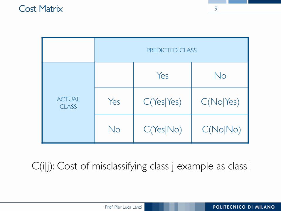
Cost Matrix 9

C(i|j): Cost of misclassifying class j example as class i

PREDICTED CLASS

ACTUAL ��CLASS

Yes No

Yes C(Yes|Yes) C(No|Yes)

No C(Yes|No) C(No|No)


Computing Cost of Classification 10

Cost Matrix PREDICTED CLASS

ACTUAL ��CLASS

C(i|j) + -+ -1 100- 1 0

Model M1 PREDICTED CLASS

��ACTUAL ��CLASS

+ -+ 150 40- 60 250

Model M2 PREDICTED CLASS

��ACTUAL ��CLASS

+ -+ 250 45- 5 200

Accuracy = 80%Cost = 3910

Accuracy = 90%Cost = 4255






Cost-Sensitive Measures

•  Precision is biased towards C(Yes|Yes) & C(Yes|No), •  Recall is biased towards C(Yes|Yes) & C(No|Yes)•  F1-measure is biased towards all except C(No|No),��

it is high when both precision and recall are reasonably high

15

The higher the precision, the lower the FPs

The higher the precision, the lower the FNs

The higher the F1, ��the lower the FPs & FNs


How to obtain reliable estimates?(Methods for Performance Evaluation)


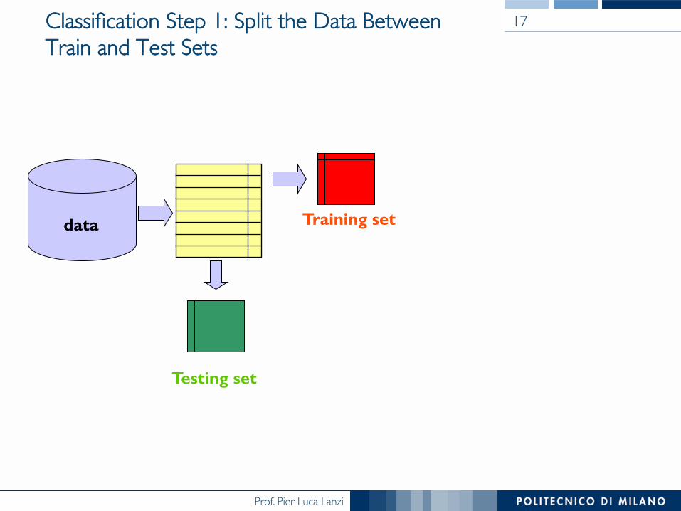
Classification Step 1: Split the Data Between Train and Test Sets

17

Training set

Testing set

data


Classification Step 2: Compute a Model using the Data in the Training Set

18

Training set

Testing set

data

Model Builder

Y N


Classification Step 3: Evaluate the Model using the Test Set

19

Training set

Testing set

data

Model Builder Predictions

Y N

Evaluate

+ - + -


Note on Parameter Tuning

•  It is important that the test data is not used ��in any way to create the classifier

•  Some learning schemes operate in two stages:§ Stage 1: builds the basic structure§ Stage 2: optimizes parameter settings

•  The test data can’t be used for parameter tuning!

•  Proper procedure uses three sets: training data, validation data, and test data. Validation data is used to optimize parameters

20


Making the most of the data

•  Once evaluation is complete, all the data can be used to build the final classifier

•  Generally, the larger the training data the better the classifier ��(but returns diminish)

•  The larger the test data the more accurate the error estimate

21


The Full Process: Training, Validation, and Testing 22

Training set

Validation set

data

Model Builder Predictions

Y N

Evaluate

+ - + -

Model Builder

Testing set

Y N

+ - + -

Final Evaluation


Methods for Performance Evaluation

•  How to obtain a reliable estimate of performance?

•  Performance of a model may depend on ��other factors besides the learning algorithm:§ Class distribution§ Cost of misclassification§ Size of training and test sets

23


Methods of Estimation

•  Holdout§ Reserve ½ for training and ½ for testing§ Reserve 2/3 for training and 1/3 for testing

•  Random subsampling§ Repeated holdout

•  Cross validation§ Partition data into k disjoint subsets§ k-fold: train on k-1 partitions, test on the remaining one§ Leave-one-out: k=n

•  Stratified sampling § oversampling vs undersampling

•  Bootstrap§ Sampling with replacement

24


Holdout Evaluation & “Small” Datasets

•  Reserves a certain amount for testing and uses the remainder for training, typically,§ Reserve ½ for training and ½ for testing§ Reserve 2/3 for training and 1/3 for testing

•  For small or “unbalanced” datasets, samples might not be representative

•  For instance, it might generate training or testing datasets with few or none instances of some classes

•  Stratified sampling § Makes sure that each class is represented with approximately equal

proportions in both subsets

25


Repeated Holdout

•  Holdout estimate can be made more reliable by repeating the process with different subsamples

•  In each iteration, a certain proportion is randomly selected for training (possibly with stratification)

•  The error rates on the different iterations are averaged to yield an overall error rate

•  Still not optimum since the different test sets overlap

26


Cross-Validation

•  First step§ Data is split into k subsets of equal size

•  Second step§ Each subset in turn is used for testing and the remainder for training

•  This is called k-fold cross-validation and avoids overlapping test sets

•  Often the subsets are stratified before cross-validation is performed

•  The error estimates are averaged to yield an overall error estimate

27


Ten-fold Crossvalidation 28

1 2 3 4 5 6 7 8 9 10

1 2 3 4 5 6 7 8 9 10test train

1 2 3 4 5 6 7 8 9 10testtrain

2 3 4 5 6 7 8 9 10test train

1train

… … …

p1

p2

p10

The final performance is computed as the average pi


Cross-Validation

•  Standard method for evaluation stratified ten-fold cross-validation

•  Why ten? Extensive experiments have shown that this is the best choice to get an accurate estimate

•  Stratification reduces the estimate’s variance

•  Even better: repeated stratified cross-validation

•  E.g. ten-fold cross-validation is repeated ten times and results are averaged (reduces the variance)

•  Other approaches appear to be robust, e.g., 5x2 crossvalidation

29


Leave-One-Out Cross-Validation

•  It is a particular form of cross-validation§ Set number of folds to number of training instances§ I.e., for n training instances, build classifier n times

•  Makes best use of the data

•  Involves no random subsampling

•  Computationally expensive

30


Leave-One-Out and Stratification

•  Disadvantage of Leave-One-Out is that: ��stratification is not possible

•  It guarantees a non-stratified sample because ��there is only one instance in the test set!

•  Extreme example: random dataset split equally into two classes§ Best inducer predicts majority class§ 50% accuracy on fresh data § Leave-One-Out-CV estimate is 100% error!

31


Bootstraping

•  Cross-validation uses sampling without replacement§ The same instance, once selected, can not be selected again for a

particular training/test set

•  Bootstrap uses sampling with replacement to form the training set§ Sample a dataset of n instances n times with ��

replacement to form a new dataset of n instances§ Use this data as the training set§ Use the instances from the original dataset that don’t occur in the new

training set for testing

32


The 0.632 Bootstrap

•  An instance has a probability of 1–1/n of not being picked

•  Thus its probability of ending up in the test data is:

•  This means the training data will contain approximately 63.2% of the instances

33

368.011 1 =≈"#$

%&' − −e

n

n


Estimating Error using Bootstrap

•  The error estimate on the test data will be very pessimistic, since training was on just ~63% of the instances

•  Therefore, combine it with the resubstitution error:

•  The resubstitution error gets less weight than the error on the test data

•  Repeat process several times with different replacement samples; average the results

34

instances traininginstancestest 368.0632.0 eeerr ⋅+⋅=


More on Bootstrap

•  Probably the best way of estimating performance for very small datasets

•  However, it has some problems§ Consider a random dataset with a 50% class distribution§ An model that memorizes all the training data (equivalent to a

kNN with k=1) will achieve 0% error on the training data��and ~50% error on test data

§ Bootstrap estimate for this classifier will be

§ But the true expected error is 50%

35

%6.31%0368.0%50632.0 =⋅+⋅=err


Model ComparisonHow to compare the relative

performance among competing models?


How to Compare the Performance of Two Models?

•  Two models, § Model M1: accuracy = 85%, tested on 30 instances§ Model M2: accuracy = 75%, tested on 5000 instances

•  Can we say M1 is better than M2?

•  How much confidence can we place on accuracy of M1 & M2?

•  Can the difference in performance measure be explained as a result of random fluctuations in the test set?

37


Confidence Interval for Accuracy

•  Prediction can be regarded as a Bernoulli trial with two possible outcomes, correct or wrong

•  A collection of Bernoulli trials has a Binomial distribution

•  Given, § the number of correct test predictions x§ the number of test instances N, § the accuracy p = s/N

•  Can we predict the true accuracy of the model from p?

38


Mean and Variance

•  Mean and variance for a Bernoulli trial is p and p(1-p)•  Expected success rate f = S/N• When N is large enough, f follows a normal distribution with

mean p and variance p(1-p)/N•  c% confidence level interval [-z ≤ X ≤z] for a random variable of

mean 0 is given by

• With a symmetric distribution, we have

39



•  For instance, if X has mean 0 and standard deviation 1, ��the confidence interval for c% is defined by the z values,

•  Thus, for the confidence interval for 90% ��we have,��

•  To compute the confidence interval for the��expected accuracy f we need to,§ Normalize it to a distribution with mean 0 and standard deviation1§ Compute the confidence interval§ Remap it to the actual distribution

40

Pr[X ≥ z] z

0.1% 3.09

0.5% 2.58

1% 2.33

5% 1.65

10% 1.28

20% 0.84

25% 0.69

40% 0.25



•  First, transform f using,

•  Compute the confidence interval,

•  Solve it for p,

41


Examples

• When f = 75%, N=1000, c=80% (z=1.28), the confidence interval for the actual performance is [0.732, 0.767]

• When f = 75%, N=100, c=80% (z=1.28), the confidence interval for the actual performance is [0.691, 0.801]

•  Note that the assumption about f being normally distributed only applies for large values of N (at least 30)

• When f = 75%, N=10, c=80% (z=1.28), the confidence interval for the actual performance is [0.0.549, 0.881]

42


Comparing Data Mining Schemes

• Which of two learning schemes performs better?

•  The answer is obviously domain-dependent

•  The typical approach is to compare10-fold cross-validation (CV) estimates using the Student’s t-test

•  Student’s t-test tells whether the means of two samples are��significantly different

•  Use a paired t-test when the individual samples are paired, that is, when the same CV is applied twice. Use unpaired t-test otherwise

43


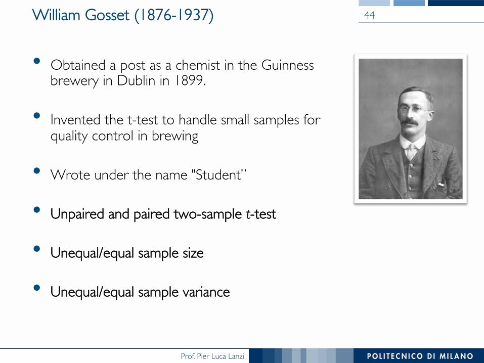
William Gosset (1876-1937)

•  Obtained a post as a chemist in the Guinness brewery in Dublin in 1899.

•  Invented the t-test to handle small samples for quality control in brewing

•  Wrote under the name "Student”

•  Unpaired and paired two-sample t-test

•  Unequal/equal sample size

•  Unequal/equal sample variance

44




T-Test Using R

> j48 <- c(96,93.33,92.00,94.67,96.00,94.00,94.67,94.0,94.67,98) > zeror <- c(33.33, 33.33, 33.33, 33.33, 33.33, 33.33, 33.33, 33.33, 33.33, 33.33) > t.test(j48,zeror)

Welch Two Sample t-test

data: j48 and zeror t = 117.9102, df = 9, p-value = 1.153e-15 alternative hypothesis: true difference in means is not equal to 0 95 percent confidence interval:

60.22594 62.58206 sample estimates: mean of x mean of y

94.734 33.330

47



ROC (Receiver Operating Characteristic)

•  Developed in 1950s for signal detection theory ��to analyze noisy signals

•  ROC curve plots TP (on the y-axis) against FP (on the x-axis), ��or TPR vs FPR (TPR = TP/(TP+FN), FPR=FP/(TN+FP))

•  Performance of each classifier represented ��as a point on the ROC curve

•  Changing the threshold of algorithm, sample distribution or cost matrix changes the location of the point

49


ROC Curve

•  (TP,FP)§ (0,0): declare everything ��

to be negative class§ (1,1): declare everything ��

to be positive class§ (1,0): ideal

•  Diagonal line:§ Random guessing§ Below diagonal line, ��

prediction is opposite ��of the true class

50


ROC Curve 51


Using ROC for Model Comparison

•  No model consistently outperform the other•  M1 is better for small FPR•  M2 is better for large FPR

•  Area Under the ROC curve•  Ideal, area = 1•  Random guess, ��

area = 0.5

52





Lift Charts

•  Lift is a measure of the effectiveness of a predictive model calculated as the ratio between the results obtained with and without the predictive model

•  Cumulative gains and lift charts are visual aids for measuring model performance

•  Both charts consist of a lift curve and a baseline

•  The greater the area between the lift curve and the baseline, the better the model

56


Example: Direct Marketing

•  Mass mailout of promotional offers (1000000)•  The proportion who normally respond is 0.1%, that is 1000

responses•  A data mining tool can identify a subset of a 100000 for which

the response rate is 0.4%, that is 400 responses•  In marketing terminology, the increase of response rate is known

as the lift factor yielded by the model.•  The same data mining tool, may be able to identify 400000

households for which the response rate is 0.2%, that is 800 respondents corresponding to a lift factor of 2.•  The overall goal is to find subsets of test instances that have a

high proportion of true positive

57


An Example from Direct Marketing 58


Which model should we prefer?(Model selection)


Model Selection Criteria

•  Model selection criteria attempt to find a good compromise between:§ The complexity of a model§ Its prediction accuracy on the training data

•  Reasoning: a good model is a simple model that achieves high accuracy on the given data•  Also known as Occam’s Razor :��

the best theory is the smallest one��that describes all the facts

60

William of Ockham, born in the village of Ockham in Surrey (England) about 1285, was the most influential philosopher of the 14th century and a controversial theologian.


The MDL principle

•  MDL stands for minimum description length•  The description length is defined as:

space required to describe a theory+

space required to describe the theory’s mistakes

•  In our case the theory is the classifier and the mistakes are the errors on the training data

• We seek a classifier with Minimum Description Language

61


MDL and compression

•  MDL principle relates to data compression

•  The best theory is the one that compresses the data the most

•  I.e. to compress a dataset we generate a model and ��then store the model and its mistakes

• We need to compute��(a) size of the model, and��(b) space needed to encode the errors

•  (b) easy: use the informational loss function•  (a) need a method to encode the model

62


Which Classification Algorithm?

•  Among the several algorithms, which one is the “best”?§ Some algorithms have a lower computational complexity§ Different algorithms provide different representations§ Some algorithms allow the specification of prior knowledge

•  If we are interested in the generalization performance, ��are there any reasons to prefer one classifier over another?

•  Can we expect any classification method to be superior or inferior overall?

•  According to the No Free Lunch Theorem, ��the answer to all these questions is known

63


No Free Lunch Theorem

•  If the goal is to obtain good generalization performance, there are no context-independent or usage-independent reasons to favor one classification method over another•  If one algorithm seems to outperform another in a certain situation, it is

a consequence of its fit to the particular problem, not the general superiority of the algorithm•  When confronting a new problem, this theorem suggests that we

should focus on the aspects that matter most§ Prior information§ Data distribution§ Amount of training data§ Cost or reward

•  The theorem also justifies skepticism regarding studies that “demonstrate” the overall superiority of a certain algorithm

64


No Free Lunch Theorem

•  "[A]ll algorithms that search for an extremum of a cost [objective] function perform exactly the same, when averaged over all possible cost functions.“ [1]

•  “[T]he average performance of any pair of algorithms across all possible problems is identical.” [2]

•  Wolpert, D.H., Macready, W.G. (1995), No Free Lunch Theorems for Search, Technical Report SFI-TR-95-02-010 (Santa Fe Institute).

•  Wolpert, D.H., Macready, W.G. (1997), No Free Lunch Theorems for Optimization, IEEE Transactions on Evolutionary Computation 1, 67.

65

Education

DMTM 2015 - 14 Evaluation of Classification Models