Embed Size (px)
Citation preview

Descriptive Statistics
Measure of Central tendency:
1. Mean2. Mod3. Median
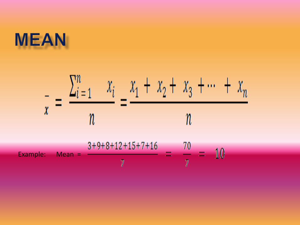
Example: Mean =

“The middle number of an array of ascending data”
Example 1: Having odd number of data
7, 3, 9, 15, 4, 21, 23, 28, 12
Step 1: arrange in ascending order:3, 4, 7, 9, 12, 15, 21, 23, 28
*The 5th data is the median
[(9+1)th divide by 2 = 5th ]
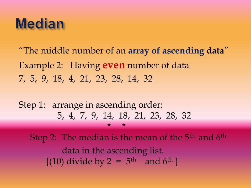
“The middle number of an array of ascending data”
Example 2: Having even number of data
7, 5, 9, 18, 4, 21, 23, 28, 14, 32
Step 1: arrange in ascending order:5, 4, 7, 9, 14, 18, 21, 23, 28, 32
* *Step 2: The median is the mean of the 5th and 6th
data in the ascending list.[(10) divide by 2 = 5th and 6th ]
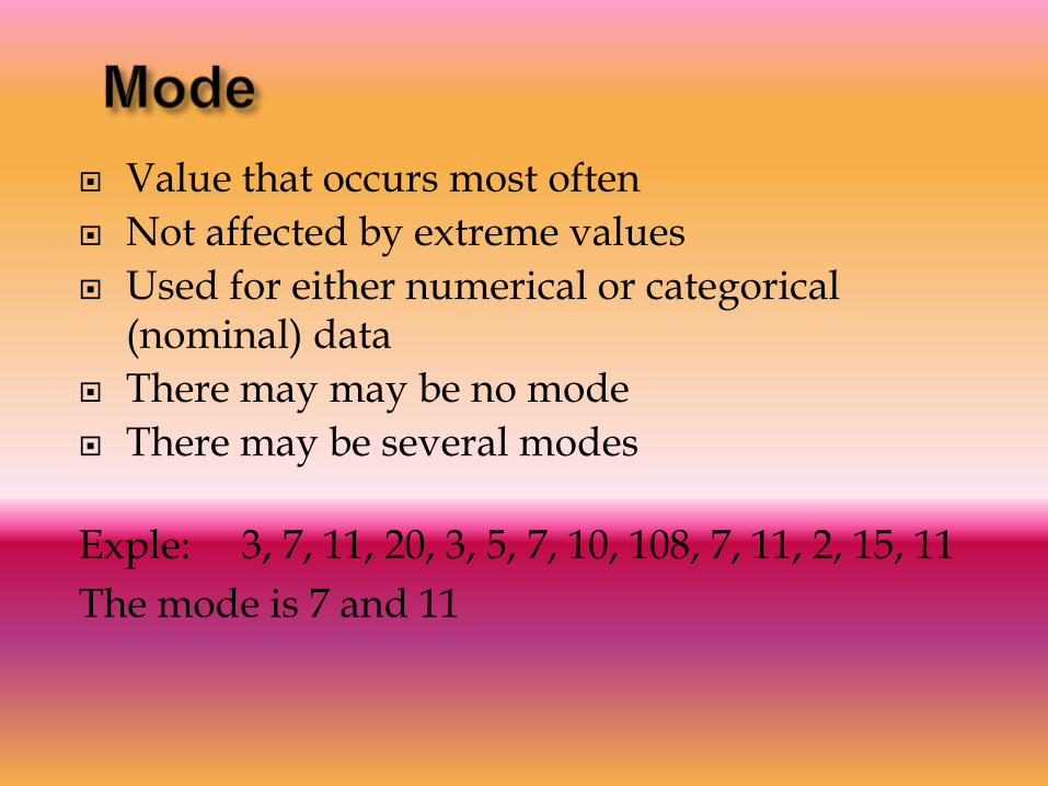
Value that occurs most often
Not affected by extreme values
Used for either numerical or categorical (nominal) data
There may may be no mode
There may be several modes
Exple: 3, 7, 11, 20, 3, 5, 7, 10, 108, 7, 11, 2, 15, 11
The mode is 7 and 11
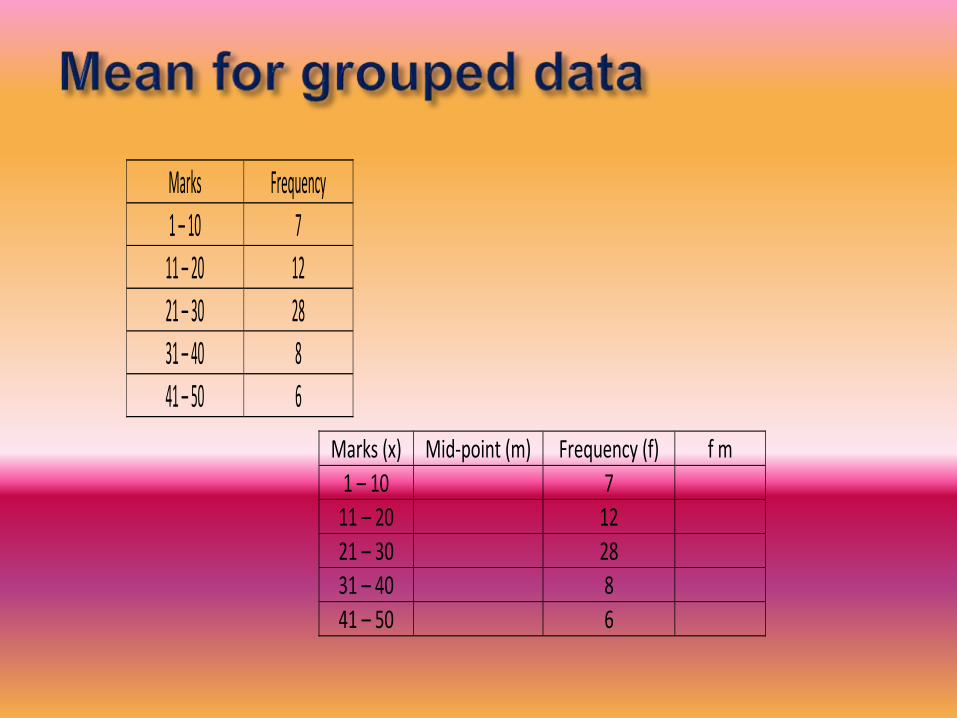
Marks Frequency
1 – 10 7 11 – 20 12
21 – 30 28 31 – 40 8
41 – 50 6
Marks (x) Mid-point (m) Frequency (f) f m
1 – 10 7 11 – 20 12
21 – 30 28 31 – 40 8
41 – 50 6
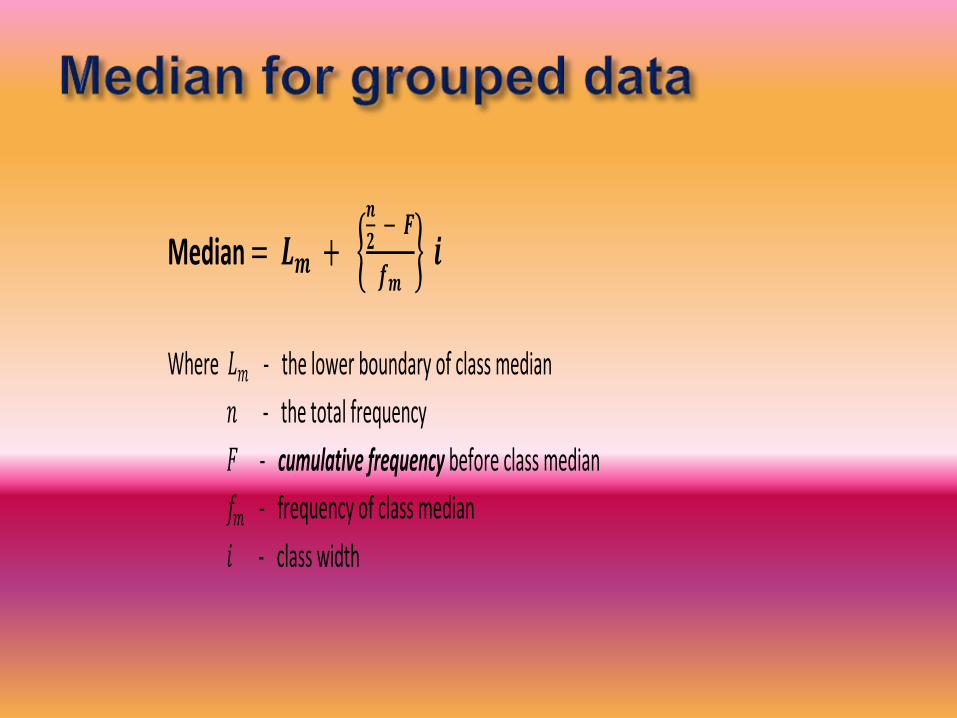
Median = 𝑳𝒎 + 𝒏
𝟐 − 𝑭
𝒇𝒎 𝒊
Where 𝐿𝑚 - the lower boundary of class median
𝑛 - the total frequency
𝐹 - cumulative frequency before class median
𝑓𝑚 - frequency of class median
𝑖 - class width
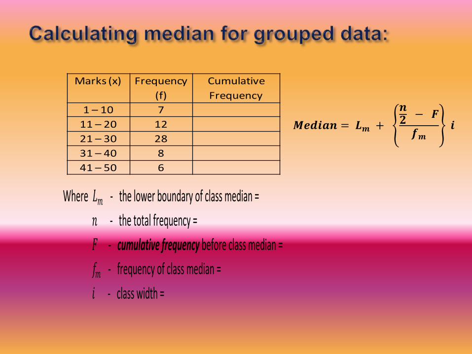
Marks (x) Frequency
(f)
Cumulative
Frequency
1 – 10 7
11 – 20 12
21 – 30 28
31 – 40 8
41 – 50 6
Where 𝐿𝑚 - the lower boundary of class median =
𝑛 - the total frequency =
𝐹 - cumulative frequency before class median =
𝑓𝑚 - frequency of class median =
𝑖 - class width =
𝑴𝒆𝒅𝒊𝒂𝒏 = 𝑳𝒎 +
𝒏𝟐 − 𝑭
𝒇𝒎 𝒊
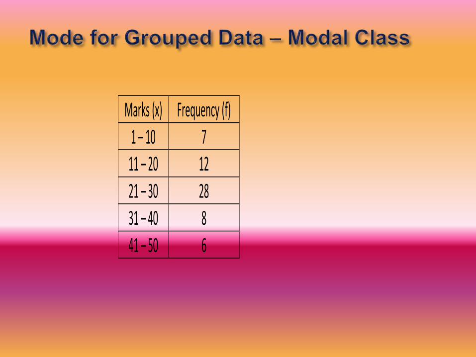
Marks (x) Frequency (f)
1 – 10 7 11 – 20 12
21 – 30 28 31 – 40 8
41 – 50 6
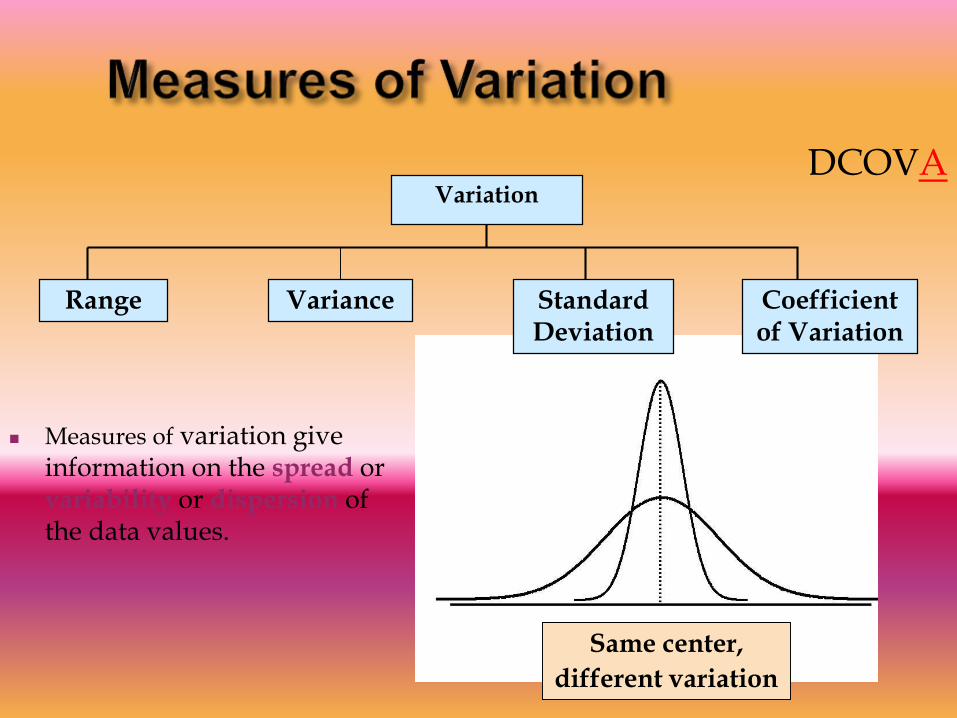
Same center,
different variation
Measures of variation give information on the spread orvariability or dispersion of the data values.
Variation
Standard Deviation
Coefficient of Variation
Range Variance
DCOVA
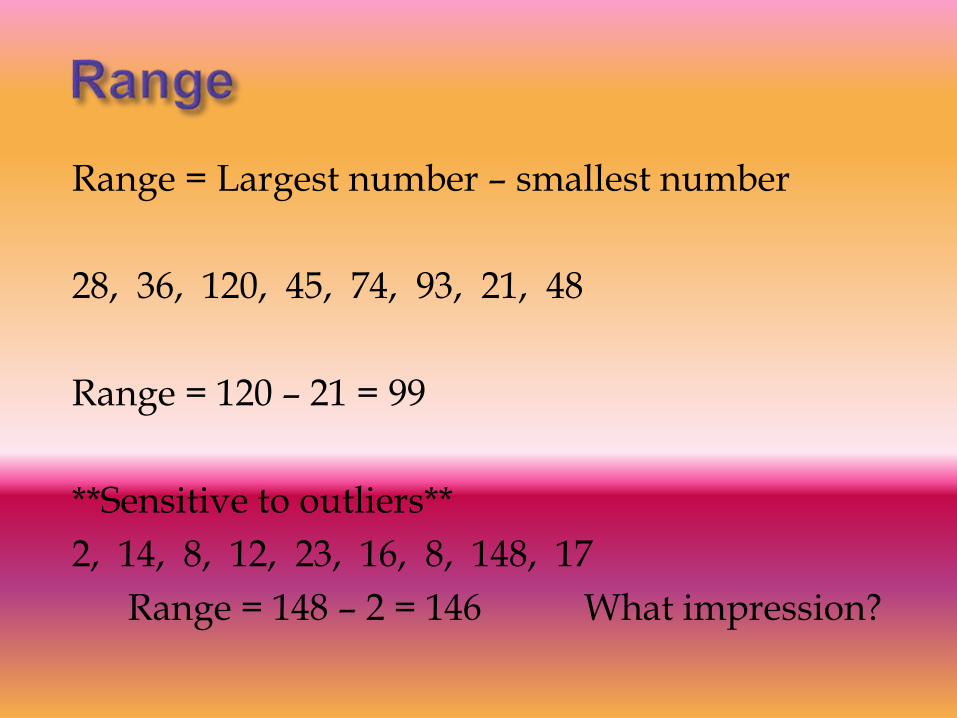
Range = Largest number – smallest number
28, 36, 120, 45, 74, 93, 21, 48
Range = 120 – 21 = 99
**Sensitive to outliers**
2, 14, 8, 12, 23, 16, 8, 148, 17
Range = 148 – 2 = 146 What impression?
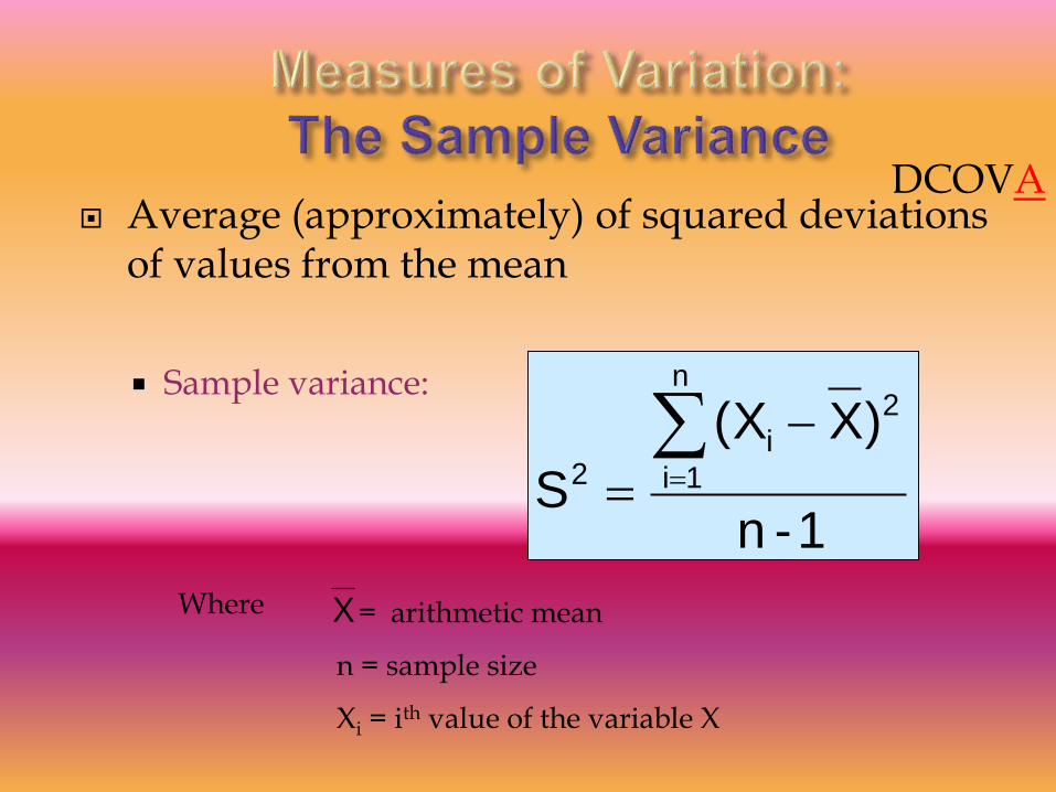
Average (approximately) of squared deviations of values from the mean
Sample variance:
1-n
)X(X
S
n
1i
2
i2
Where = arithmetic mean
n = sample size
Xi = ith value of the variable X
X
DCOVA
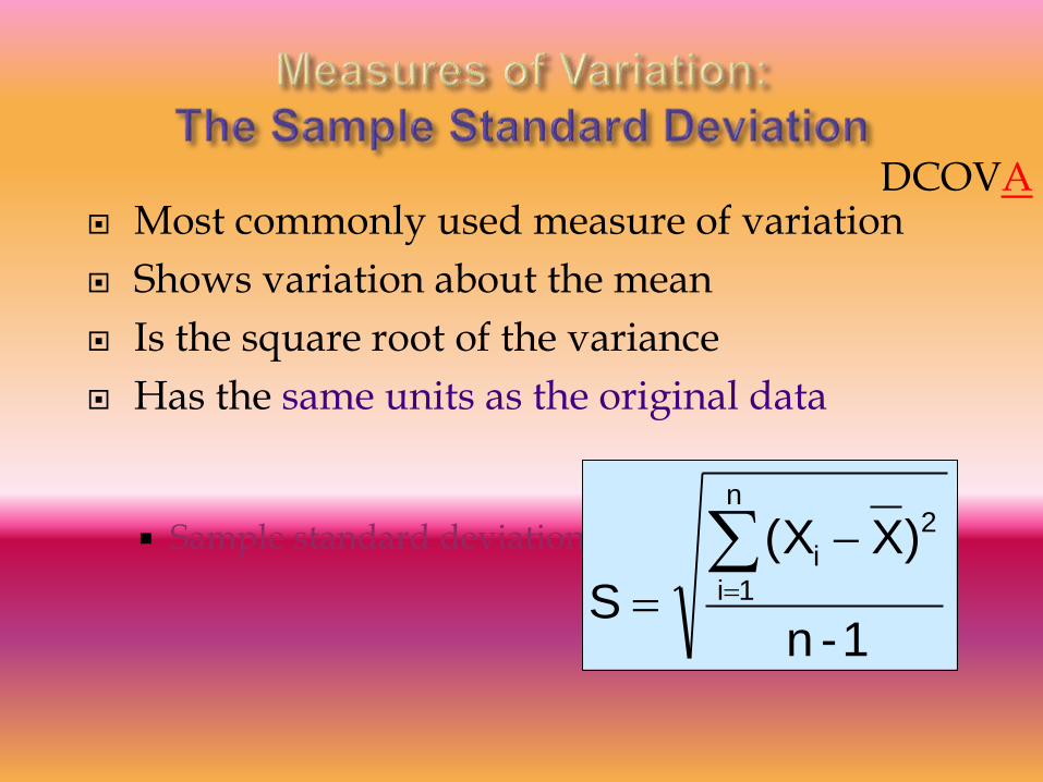
Most commonly used measure of variation
Shows variation about the mean
Is the square root of the variance
Has the same units as the original data
Sample standard deviation:
1-n
)X(X
S
n
1i
2
i
DCOVA
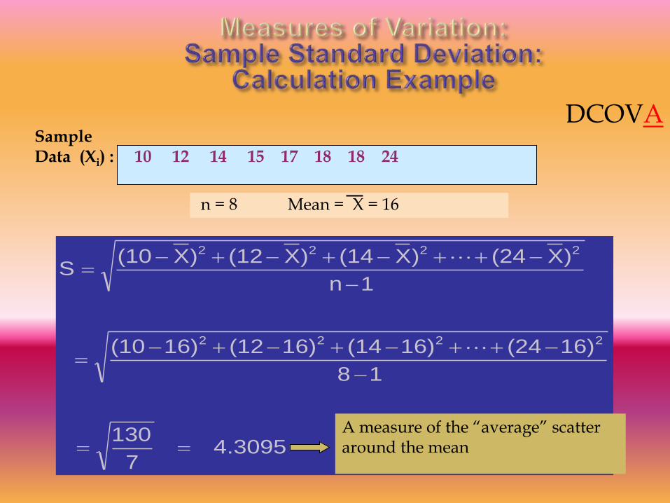
Sample Data (Xi) : 10 12 14 15 17 18 18 24
n = 8 Mean = X = 16
4.30957
130
18
16)(2416)(1416)(1216)(10
1n
)X(24)X(14)X(12)X(10S
2222
2222
A measure of the “average” scatter around the mean
DCOVA
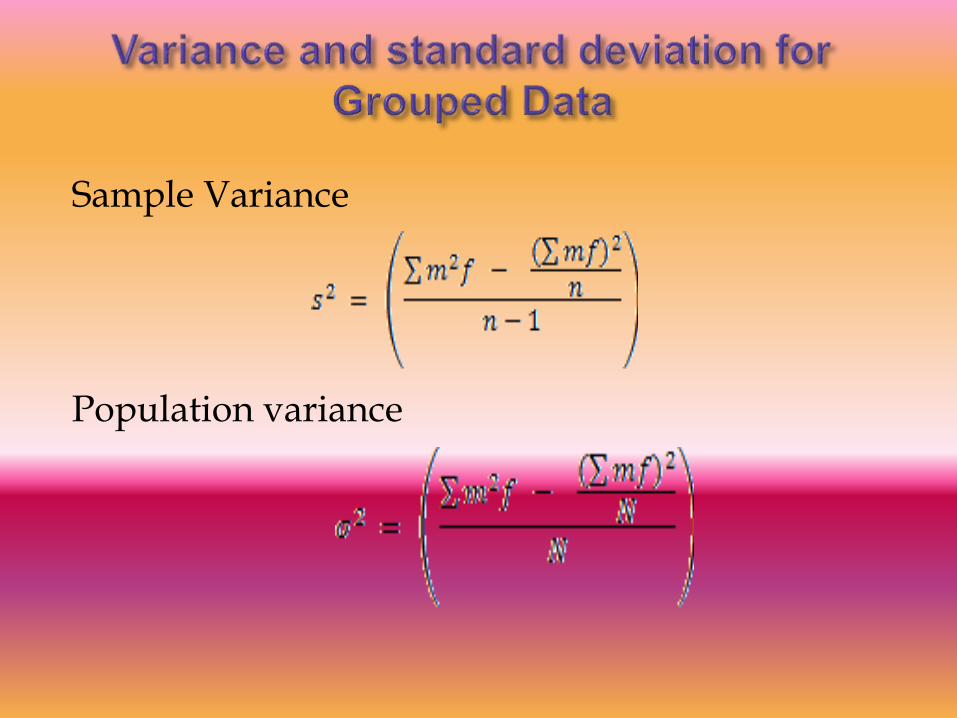
Sample Variance
Population variance
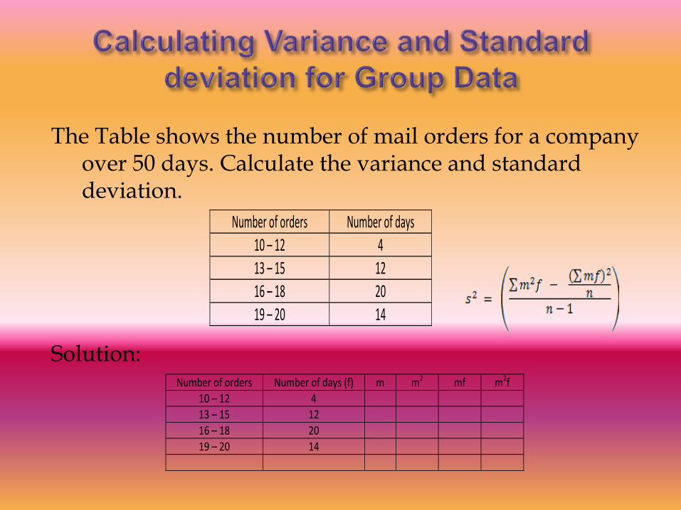
The Table shows the number of mail orders for a company over 50 days. Calculate the variance and standard deviation.
Solution:
Number of orders Number of days
10 – 12 4
13 – 15 12
16 – 18 20
19 – 20 14
Number of orders Number of days (f) m m2 mf m2f
10 – 12 4
13 – 15 12
16 – 18 20
19 – 20 14
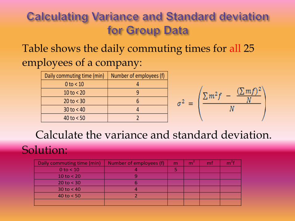
Table shows the daily commuting times for all 25
employees of a company:
Calculate the variance and standard deviation.
Solution:
Daily commuting time (min) Number of employees (f)
0 to < 10 4
10 to < 20 9
20 to < 30 6
30 to < 40 4
40 to < 50 2
Daily commuting time (min) Number of employees (f) m m2 mf m2f
0 to < 10 4 5
10 to < 20 9
20 to < 30 6
30 to < 40 4
40 to < 50 2
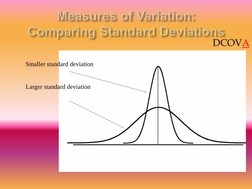
Smaller standard deviation
Larger standard deviation
DCOVA
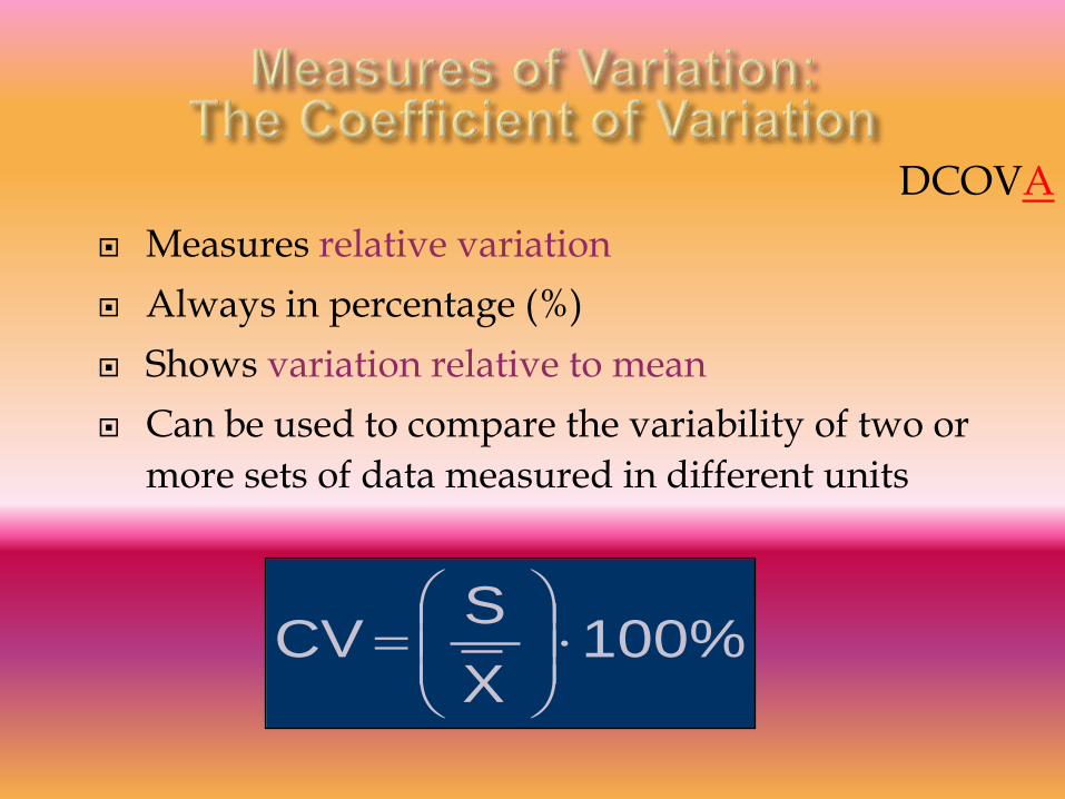
Measures relative variation
Always in percentage (%)
Shows variation relative to mean
Can be used to compare the variability of two or
more sets of data measured in different units
100%X
SCV
DCOVA
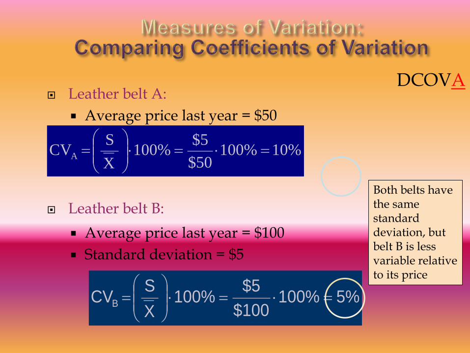
Leather belt A:
Average price last year = $50
Standard deviation = $5
Leather belt B:
Average price last year = $100
Standard deviation = $5
Both belts have the same standard deviation, but belt B is less variable relative to its price
10%100%$50
$5100%
X
SCVA
5%100%$100
$5100%
X
SCVB
DCOVA
To compute the Z-score of a data value, subtract the mean and divide by the standard deviation.
The Z-score is the number of standard deviations a data value is from the mean.
A data value is considered an extreme outlier if its Z-score is less than -3.0 or greater than +3.0.
The larger the absolute value of the Z-score, the farther the data value is from the mean.
DCOVA
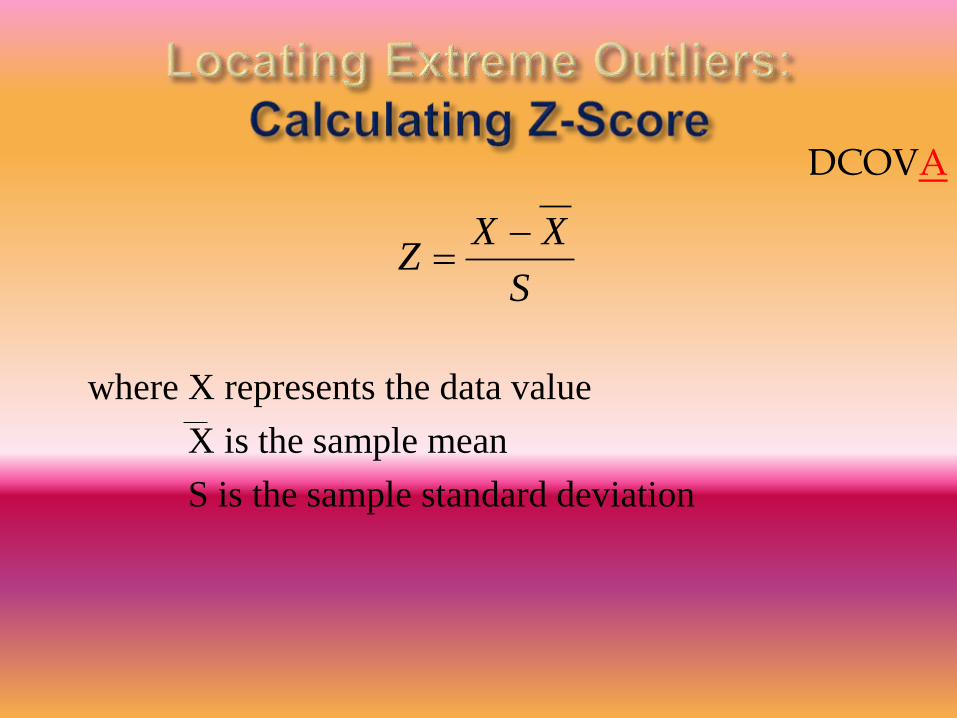
where X represents the data value
X is the sample mean
S is the sample standard deviation
S
XXZ
DCOVA
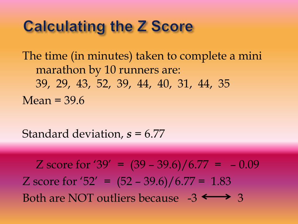
The time (in minutes) taken to complete a mini marathon by 10 runners are:39, 29, 43, 52, 39, 44, 40, 31, 44, 35
Mean = 39.6
Standard deviation, s = 6.77
Z score for ‘39’ = (39 – 39.6)/6.77 = – 0.09
Z score for ‘52’ = (52 – 39.6)/6.77 = 1.83
Both are NOT outliers because -3 3
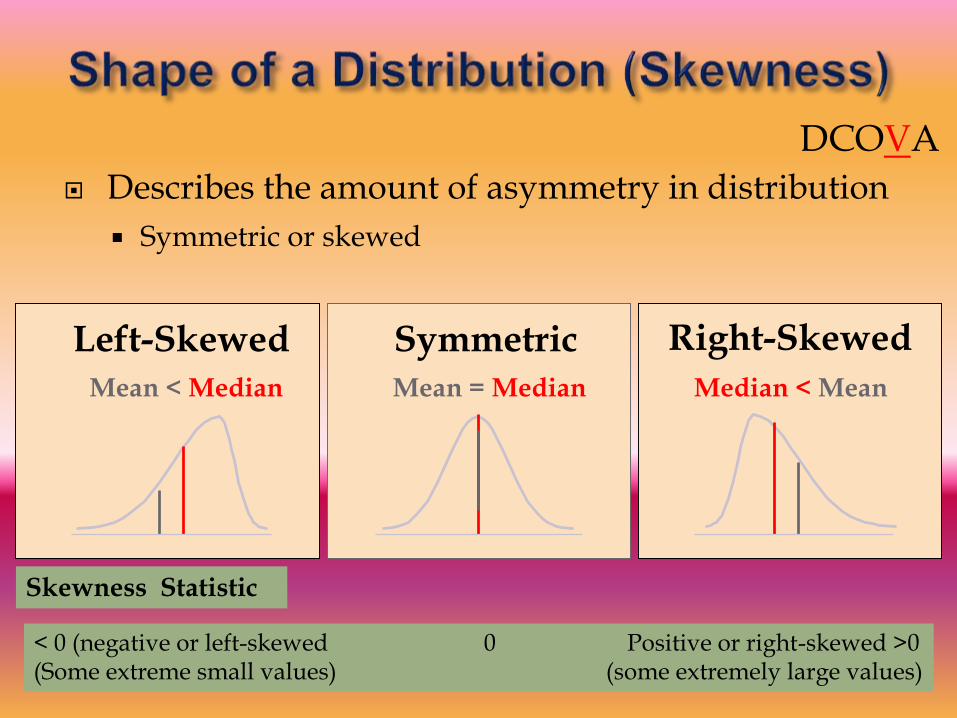
Describes the amount of asymmetry in distribution
Symmetric or skewed
Mean = MedianMean < Median Median < Mean
Right-SkewedLeft-Skewed Symmetric
DCOVA
Skewness Statistic
< 0 (negative or left-skewed 0 Positive or right-skewed >0(Some extreme small values) (some extremely large values)
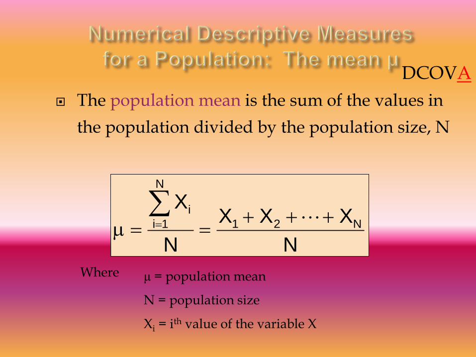
The population mean is the sum of the values in
the population divided by the population size, N
N
XXX
N
XN21
N
1i
i
μ = population mean
N = population size
Xi = ith value of the variable X
Where
DCOVA

Average of squared deviations of values from the mean
Population variance:
N
μ)(X
σ
N
1i
2
i2
Where μ = population mean
N = population size
Xi = ith value of the variable X
DCOVA
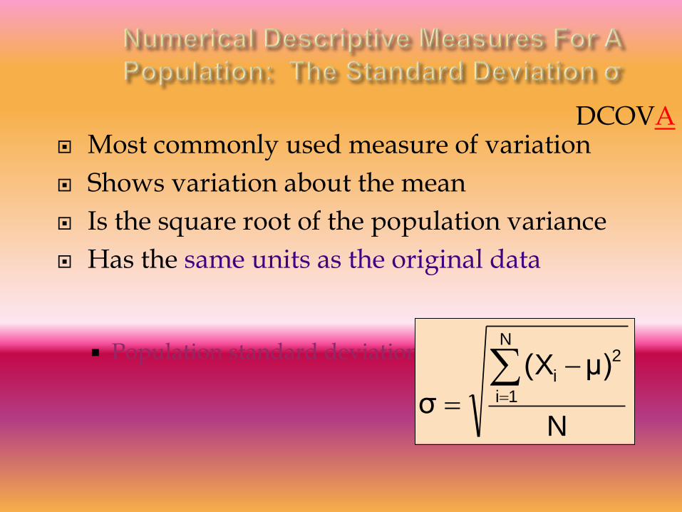
Most commonly used measure of variation
Shows variation about the mean
Is the square root of the population variance
Has the same units as the original data
Population standard deviation:
N
μ)(X
σ
N
1i
2
i
DCOVA
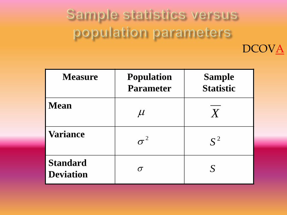
Measure Population
Parameter
Sample
Statistic
Mean
Variance
Standard
Deviation
X
2S
S
2
DCOVA
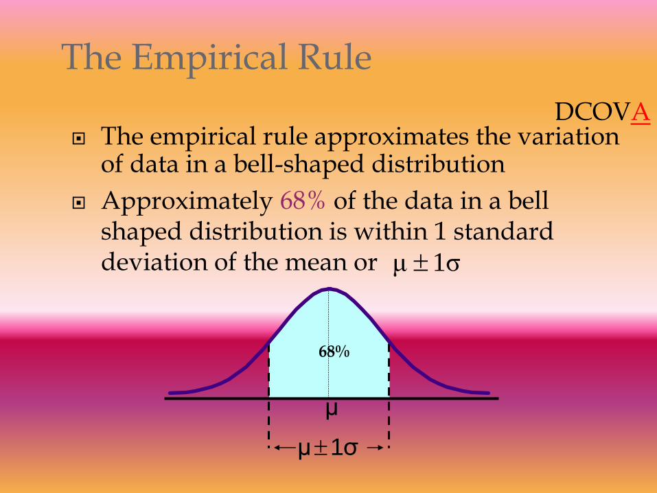
The empirical rule approximates the variation of data in a bell-shaped distribution
Approximately 68% of the data in a bell shaped distribution is within 1 standard deviation of the mean or
The Empirical Rule
1σμ
μ
68%
1σμ
DCOVA
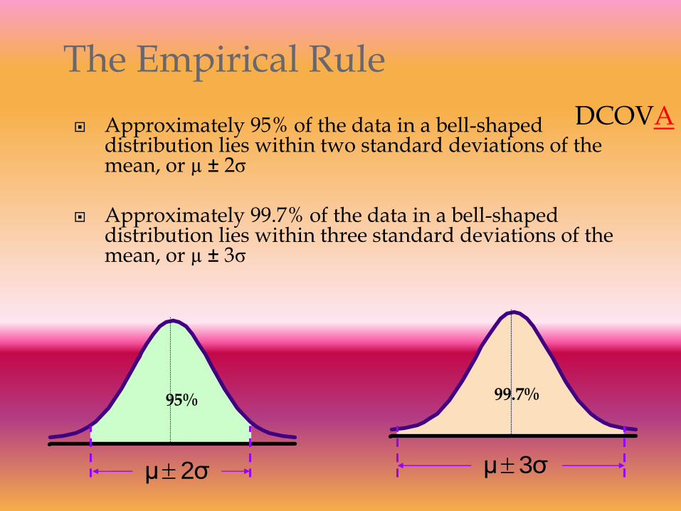
Approximately 95% of the data in a bell-shaped distribution lies within two standard deviations of the mean, or µ ± 2σ
Approximately 99.7% of the data in a bell-shaped distribution lies within three standard deviations of the mean, or µ ± 3σ
The Empirical Rule
3σμ
99.7%95%
2σμ
DCOVA

Suppose that the variable Math SAT scores is bell-shaped with a mean of 500 and a standard deviation of 90. Then,
68% of all test takers scored between 410 and 590 (500 ± 90). [1 standard deviation]
95% of all test takers scored between 320 and 680 (500 ± 180). [2 standard deviation]
99.7% of all test takers scored between 230 and 770 (500 ± 270). [3 standard deviation]
DCOVA
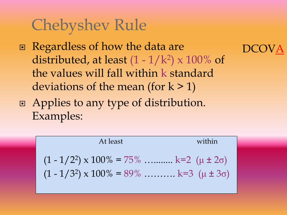
Regardless of how the data are distributed, at least (1 - 1/k2) x 100% of the values will fall within k standard deviations of the mean (for k > 1)
Applies to any type of distribution.Examples:
(1 - 1/22) x 100% = 75% …........ k=2 (μ ± 2σ)
(1 - 1/32) x 100% = 89% ………. k=3 (μ ± 3σ)
Chebyshev Rule
withinAt least
DCOVA
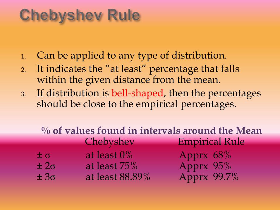
1. Can be applied to any type of distribution.
2. It indicates the “at least” percentage that falls within the given distance from the mean.
3. If distribution is bell-shaped, then the percentages should be close to the empirical percentages.
% of values found in intervals around the MeanChebyshev Empirical Rule
± σ at least 0% Apprx 68%± 2σ at least 75% Apprx 95%± 3σ at least 88.89% Apprx 99.7%

Quartiles split the ranked data into 4 segments with an equal number of values per segment
25%
The first quartile, Q1, is the value for which 25% of the observations are smaller and 75% are larger
Q2 is the same as the median (50% of the observations are smaller and 50% are larger)
Only 25% of the observations are greater than the third quartile
Q1 Q2 Q3
25% 25% 25%
DCOVA
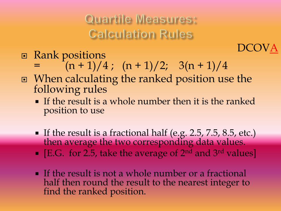
Rank positions = (n + 1)/4 ; (n + 1)/2; 3(n + 1)/4
When calculating the ranked position use the following rules If the result is a whole number then it is the ranked
position to use
If the result is a fractional half (e.g. 2.5, 7.5, 8.5, etc.) then average the two corresponding data values.
[E.G. for 2.5, take the average of 2nd and 3rd values]
If the result is not a whole number or a fractional half then round the result to the nearest integer to find the ranked position.
DCOVA
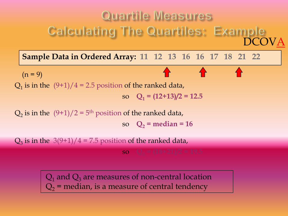
(n = 9)
Q1 is in the (9+1)/4 = 2.5 position of the ranked data,
so Q1 = (12+13)/2 = 12.5
Q2 is in the (9+1)/2 = 5th position of the ranked data,
so Q2 = median = 16
Q3 is in the 3(9+1)/4 = 7.5 position of the ranked data,
so Q3 = (18+21)/2 = 19.5
Sample Data in Ordered Array: 11 12 13 16 16 17 18 21 22
Q1 and Q3 are measures of non-central locationQ2 = median, is a measure of central tendency
DCOVA
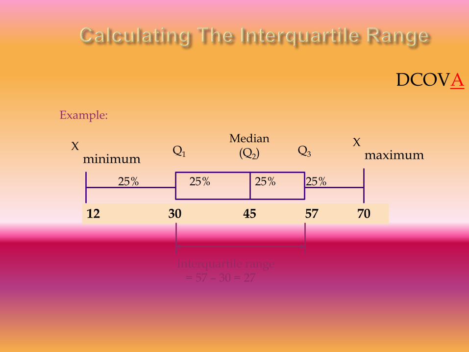
Median(Q2)
Xmaximum
Xminimum
Q1 Q3
Example:
25% 25% 25% 25%
12 30 45 57 70
Interquartile range = 57 – 30 = 27
DCOVA
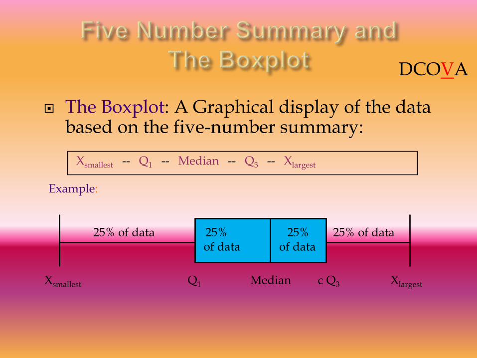
The Boxplot: A Graphical display of the data based on the five-number summary:
Example:
Xsmallest -- Q1 -- Median -- Q3 -- Xlargest
25% of data 25% 25% 25% of dataof data of data
Xsmallest Q1 Median c Q3 Xlargest
DCOVA

If data are symmetric around the median then the box and central line are centered between the endpoints
A Boxplot can be shown in either a vertical or horizontal orientation
Xsmallest Q1 Median Q3 Xlargest
DCOVA

Right-SkewedLeft-Skewed Symmetric
Q1 Q2 Q3 Q1 Q2 Q3Q1 Q2 Q3
DCOVA
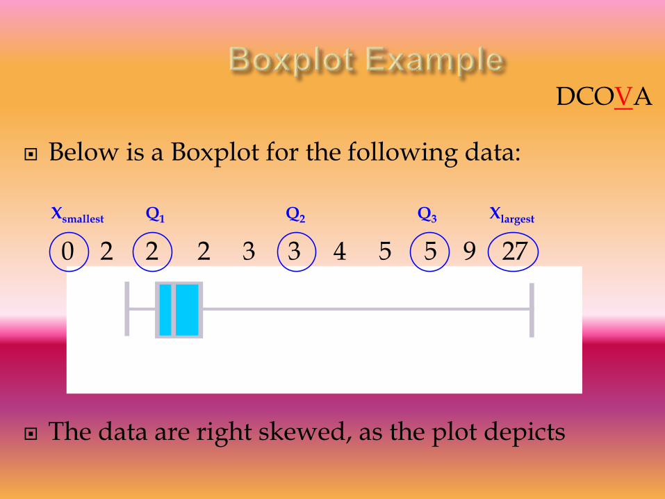
Below is a Boxplot for the following data:
0 2 2 2 3 3 4 5 5 9 27
The data are right skewed, as the plot depicts
0 2 3 5 27
Xsmallest Q1 Q2 Q3 Xlargest
DCOVA
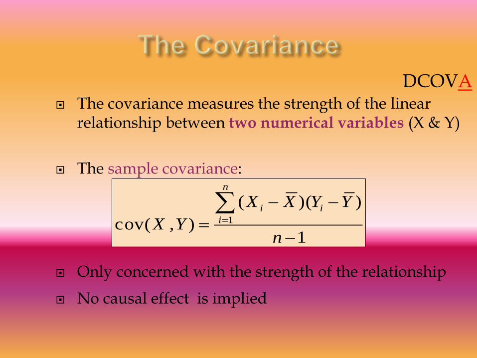
The covariance measures the strength of the linear relationship between two numerical variables (X & Y)
The sample covariance:
Only concerned with the strength of the relationship
No causal effect is implied
1
))((
),(cov 1
n
YYXX
YX
n
i
ii
DCOVA
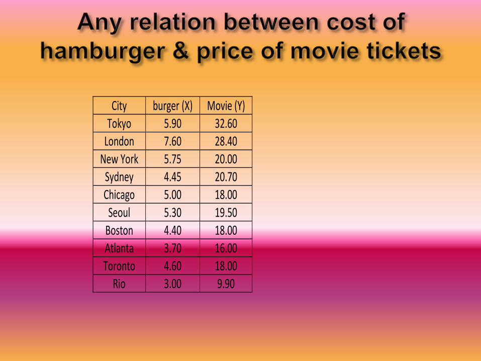
City burger (X) Movie (Y)
Tokyo 5.90 32.60
London 7.60 28.40
New York 5.75 20.00
Sydney 4.45 20.70
Chicago 5.00 18.00
Seoul 5.30 19.50
Boston 4.40 18.00
Atlanta 3.70 16.00
Toronto 4.60 18.00
Rio 3.00 9.90
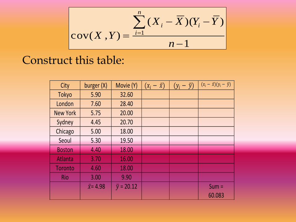
Construct this table:
1
))((
),(cov 1
n
YYXX
YX
n
i
ii
City burger (X) Movie (Y) (𝑥𝑖 − 𝑥 ) (𝑦𝑖 − 𝑦 ) (𝑥𝑖 − 𝑥 )(𝑦𝑖 − 𝑦 )
Tokyo 5.90 32.60
London 7.60 28.40
New York 5.75 20.00
Sydney 4.45 20.70
Chicago 5.00 18.00
Seoul 5.30 19.50
Boston 4.40 18.00
Atlanta 3.70 16.00
Toronto 4.60 18.00
Rio 3.00 9.90
𝑥 = 4.98 𝑦 = 20.12 Sum = 60.083
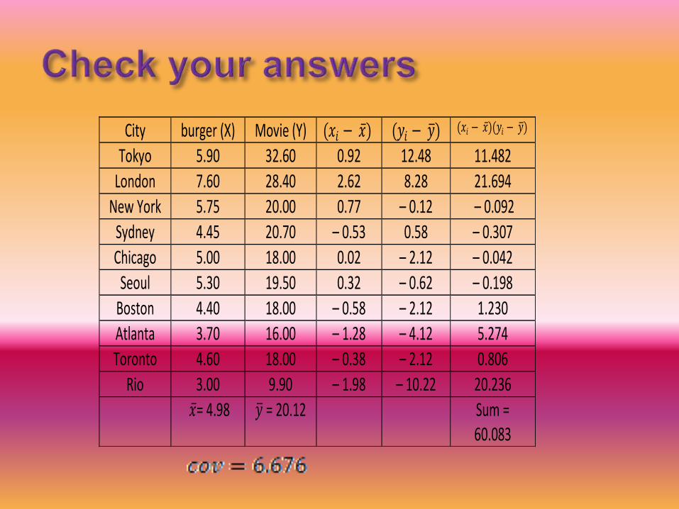
City burger (X) Movie (Y) (𝑥𝑖 − 𝑥 ) (𝑦𝑖 − 𝑦 ) (𝑥𝑖 − 𝑥 )(𝑦𝑖 − 𝑦 )
Tokyo 5.90 32.60 0.92 12.48 11.482
London 7.60 28.40 2.62 8.28 21.694
New York 5.75 20.00 0.77 – 0.12 – 0.092
Sydney 4.45 20.70 – 0.53 0.58 – 0.307
Chicago 5.00 18.00 0.02 – 2.12 – 0.042
Seoul 5.30 19.50 0.32 – 0.62 – 0.198
Boston 4.40 18.00 – 0.58 – 2.12 1.230
Atlanta 3.70 16.00 – 1.28 – 4.12 5.274
Toronto 4.60 18.00 – 0.38 – 2.12 0.806
Rio 3.00 9.90 – 1.98 – 10.22 20.236
𝑥 = 4.98 𝑦 = 20.12 Sum = 60.083
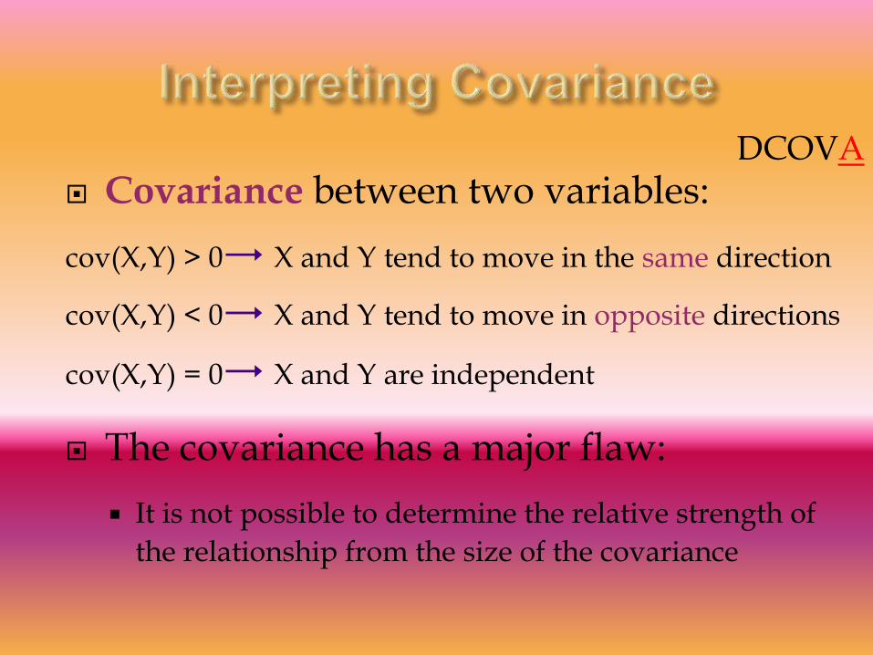
Covariance between two variables:
cov(X,Y) > 0 X and Y tend to move in the same direction
cov(X,Y) < 0 X and Y tend to move in opposite directions
cov(X,Y) = 0 X and Y are independent
The covariance has a major flaw:
It is not possible to determine the relative strength of
the relationship from the size of the covariance
DCOVA
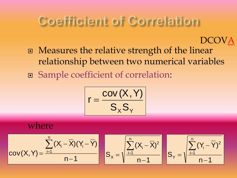
Measures the relative strength of the linear relationship between two numerical variables
Sample coefficient of correlation:
where
YXSS
Y),(Xcovr
1n
)X(X
S
n
1i
2
i
X
1n
)Y)(YX(X
Y),(Xcov
n
1i
ii
1n
)Y(Y
S
n
1i
2
i
Y
DCOVA
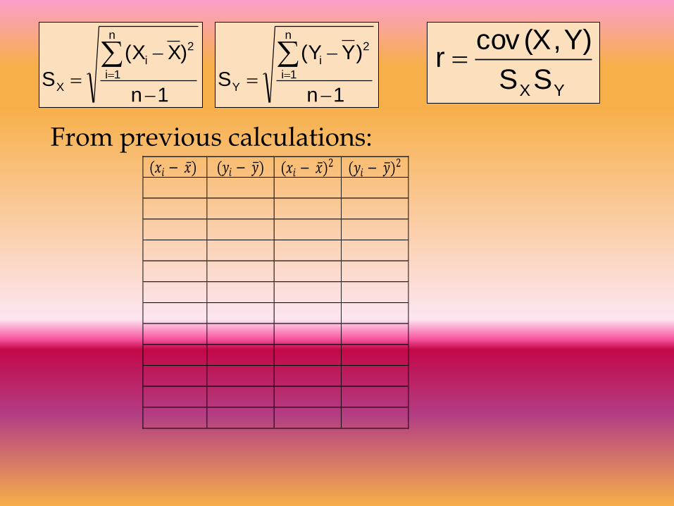
From previous calculations:
1n
)X(X
S
n
1i
2
i
X
1n
)Y(Y
S
n
1i
2
i
Y
YXSS
Y),(Xcovr
(𝑥𝑖 − 𝑥 ) (𝑦𝑖 − 𝑦 ) (𝑥𝑖 − 𝑥 )2 (𝑦𝑖 − 𝑦 )2
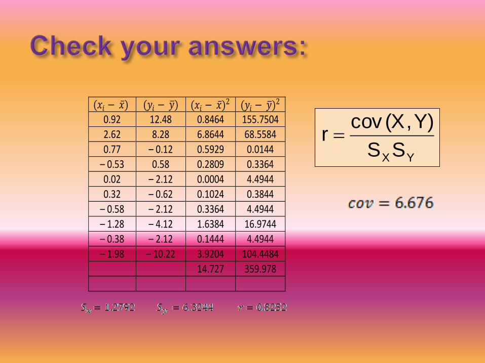
(𝑥𝑖 − 𝑥 ) (𝑦𝑖 − 𝑦 ) (𝑥𝑖 − 𝑥 )2 (𝑦𝑖 − 𝑦 )2 0.92 12.48 0.8464 155.7504
2.62 8.28 6.8644 68.5584
0.77 – 0.12 0.5929 0.0144
– 0.53 0.58 0.2809 0.3364
0.02 – 2.12 0.0004 4.4944
0.32 – 0.62 0.1024 0.3844
– 0.58 – 2.12 0.3364 4.4944
– 1.28 – 4.12 1.6384 16.9744
– 0.38 – 2.12 0.1444 4.4944
– 1.98 – 10.22 3.9204 104.4484
14.727 359.978
YXSS
Y),(Xcovr
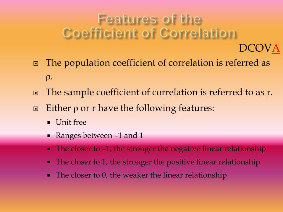
The population coefficient of correlation is referred as
ρ.
The sample coefficient of correlation is referred to as r.
Either ρ or r have the following features:
Unit free
Ranges between –1 and 1
The closer to –1, the stronger the negative linear relationship
The closer to 1, the stronger the positive linear relationship
The closer to 0, the weaker the linear relationship
DCOVA

Y
X
Y
X
Y
X
Y
X
r = -1 r = -.6
r = +.3r = +1
Y
X
r = 0
DCOVA