Data Preprocessing

.

Why Data Preprocessing?Data in the real world is dirty

incomplete: missing attribute values, lack of certain attributes of interest, or containing only aggregate data

• e.g., occupation=“”

noisy: containing errors or outliers• e.g., Salary=“-10”

inconsistent: containing discrepancies in codes or names

• e.g., Age=“42” Birthday=“03/07/1997”• e.g., Was rating “1,2,3”, now rating “A, B, C”• e.g., discrepancy between duplicate records

Why Is Data Preprocessing Important?

No quality data, no quality mining results!Quality decisions must be based on quality data

• e.g., duplicate or missing data may cause incorrect or even misleading statistics.

Data preparation, cleaning, and transformation comprises the majority of the work in a data mining application (90%).

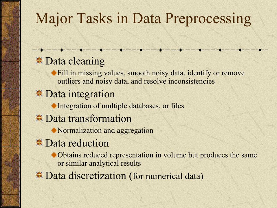
Major Tasks in Data Preprocessing

Data cleaningFill in missing values, smooth noisy data, identify or remove outliers and noisy data, and resolve inconsistencies

Data integrationIntegration of multiple databases, or files

Data transformationNormalization and aggregation

Data reductionObtains reduced representation in volume but produces the same or similar analytical results

Data discretization (for numerical data)

Data CleaningImportance

“Data cleaning is the number one problem in data warehousing”

Data cleaning tasks – this routine attempts to

Fill in missing values

Identify outliers and smooth out noisy data

Correct inconsistent data

Resolve redundancy caused by data integration

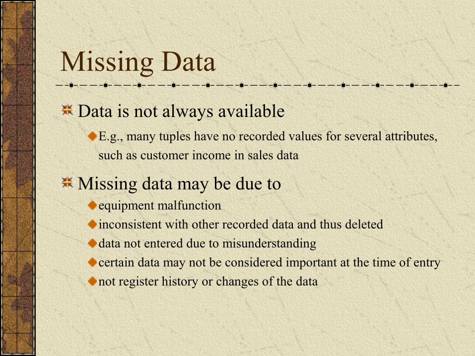
Missing Data

Data is not always availableE.g., many tuples have no recorded values for several attributes,

such as customer income in sales data

Missing data may be due to equipment malfunction

inconsistent with other recorded data and thus deleted

data not entered due to misunderstanding

certain data may not be considered important at the time of entry

not register history or changes of the data

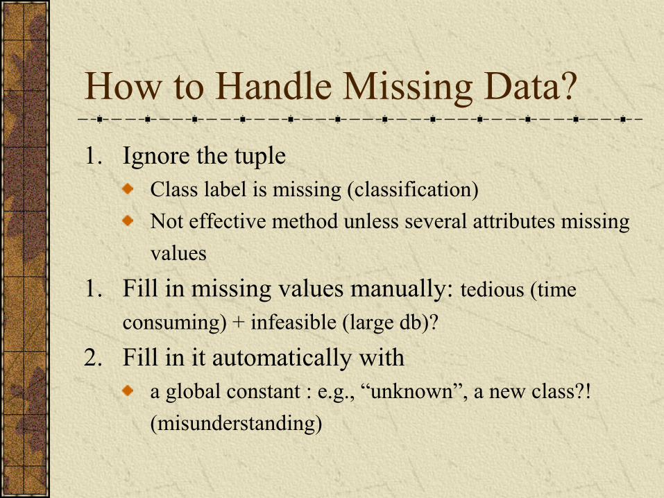
How to Handle Missing Data?

1. Ignore the tuple Class label is missing (classification)

Not effective method unless several attributes missing

values

1. Fill in missing values manually: tedious (time

consuming) + infeasible (large db)?

2. Fill in it automatically witha global constant : e.g., “unknown”, a new class?!

(misunderstanding)

Cont’d

4. the attribute mean Average income of AllElectronics customer $28,000

(use this value to replace)

5. The attribute mean for all samples belonging to

the same class as the given tuple

6. the most probable valuedetermined with regression, inference-based such as

Bayesian formula, decision tree. (most popular)

Noisy DataNoise: random error or variance in a measured variable.Incorrect attribute values may due to

faulty data collection instrumentsdata entry problemsdata transmission problemsetc

Other data problems which requires data cleaningduplicate records, incomplete data, inconsistent data

How to Handle Noisy Data?Binning method:

first sort data and partition into (equi-depth) binsthen one can smooth by bin means, smooth by bin median, smooth by bin boundaries, etc.

ClusteringSimilar values are organized into groups (clusters).Values that fall outside of clusters considered outliers.

Combined computer and human inspectiondetect suspicious values and check by human (e.g., deal with possible outliers)

RegressionData can be smoothed by fitting the data to a function such as with regression. (linear regression/multiple linear regression)

Binning Methods for Data Smoothing

Sorted data for price (in dollars): 4, 8, 15, 21, 21, 24, 25, 28, 34Partition into (equi-depth) bins:

Bin 1: 4, 8, 15Bin 2: 21, 21, 24Bin 3: 25, 28, 34

Smoothing by bin means:Bin 1: 9, 9, 9Bin 2: 22, 22, 22Bin 3: 29, 29, 29

Smoothing by bin boundaries:Bin 1: 4, 4, 15Bin 2: 21, 21, 24Bin 3: 25, 25, 34

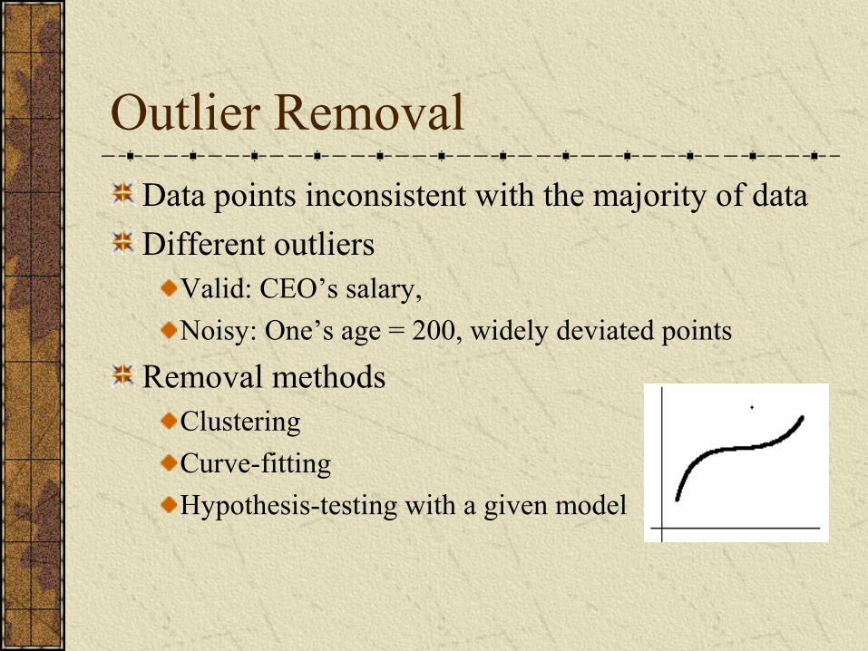
Outlier Removal

Data points inconsistent with the majority of data

Different outliersValid: CEO’s salary,

Noisy: One’s age = 200, widely deviated points

Removal methodsClustering

Curve-fitting

Hypothesis-testing with a given model

Data IntegrationData integration:

combines data from multiple sources(data cubes, multiple db or flat files)

Issues during data integrationSchema integration

• integrate metadata (about the data) from different sources• Entity identification problem: identify real world entities from

multiple data sources, e.g., A.cust-id ≡ B.cust-#(same entity?)Detecting and resolving data value conflicts

• for the same real world entity, attribute values from different sources are different, e.g., different scales, metric vs. British units

Removing duplicates and redundant data• An attribute can be derived from another table (annual

revenue)• Inconsistencies in attribute naming

Data Transformation

Smoothing: remove noise from data (binning, clustering, regression)

Normalization: scaled to fall within a small, specified range such as –1.0 to 1.0 or 0.0 to 1.0

Attribute/feature construction

New attributes constructed / added from the given ones

Aggregation: summarization or aggregation operations apply to data

Generalization: concept hierarchy climbing

Low level/ primitive/raw data are replace by higher level concepts

Data Transformation: Normalization

Useful for classification algorithms involvingNeural networksDistance measurements (nearest neighbor)

Backpropagation algorithm (NN) – normalizing help in speed up the learning phaseDistance-based methods – normalization prevent attributes with initially large range (i.e. income) from outweighing attributes with initially smaller ranges (i.e. binary attribute)

Data Transformation: Normalization

min-max normalization

z-score normalization

normalization by decimal scaling

AAA

AA

A

minnewminnewmaxnewminmax

minvv _)__(' +−

−−=

A

A

devstand

meanvv

_'

−=

j

vv

10'= Where j is the smallest integer such that Max(| |)<1'v

Example:

Suppose that the minimum and maximum values for the attribute income are $12,000 and $98,000, respectively. We would like to map income to the range [0.0, 1.0].

Suppose that the mean and standard deviation of the values for the attribute income are $54,000 and $16,000, respectively.

Suppose that the recorded values of A range from –986 to 917.

Data Reduction Strategies

Data is too big to work with – may takes time, impractical or infeasible analysis

Data reduction techniquesObtain a reduced representation of the data set that is much smaller in volume but yet produce the same (or almost the same) analytical results

Data reduction strategiesData cube aggregation – apply aggregation operations (data cube)

Cont’dDimensionality reduction—remove unimportant attributes

Data compression – encoding mechanism used to reduce data size

Numerosity reduction – data replaced or estimated by alternative, smaller data representation - parametric model (store model parameter instead of actual data), non-parametric (clustering sampling, histogram)

Discretization and concept hierarchy generation – replaced by ranges or higher conceptual levels

Data Cube Aggregation

Store multidimensional aggregated information

Provide fast access to precomputed, summarized data – benefiting on-line analytical processing and data mining

Fig. 3.4 and 3.5

Dimensionality ReductionFeature selection (i.e., attribute subset selection):

Select a minimum set of attributes (features) that is sufficient for the data mining task. Best/worst attributes are determined using test of statistical significance – information gain (building decision tree for classification)

Heuristic methods (due to exponential # of choices – 2d):

step-wise forward selectionstep-wise backward eliminationcombining forward selection and backward eliminationetc

Decision tree inductionOriginally for classificationInternal node denotes a test on an attributeEach branch corresponds to an outcome of the testLeaf node denotes a class predictionAt each node – algorithm chooses the ‘best attribute to partition the data into individual classesIn attribute subset selection – it is constructed from given data

Data Compression

Compressed representation of the original dataOriginal data can be reconstructed from compressed data (without loss of info – lossless, approximate - lossy)Two popular and effective of lossy method:

Wavelet TransformsPrinciple Component Analysis (PCA)

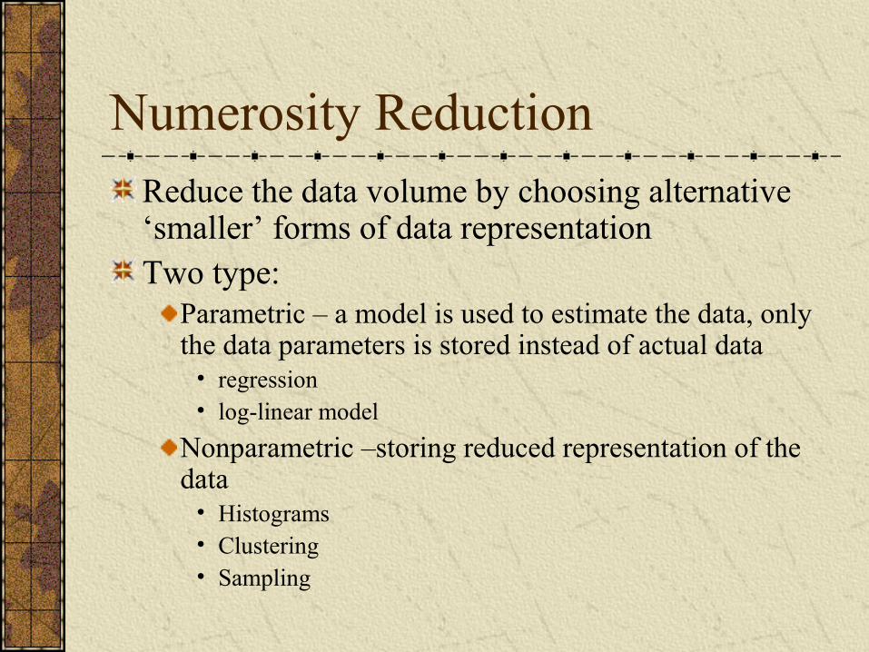
Numerosity ReductionReduce the data volume by choosing alternative ‘smaller’ forms of data representationTwo type:

Parametric – a model is used to estimate the data, only the data parameters is stored instead of actual data

• regression• log-linear model

Nonparametric –storing reduced representation of the data

• Histograms• Clustering• Sampling

Regression

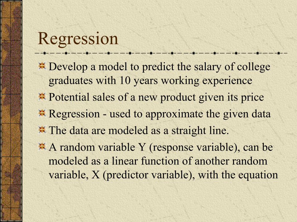
Develop a model to predict the salary of college graduates with 10 years working experience

Potential sales of a new product given its price

Regression - used to approximate the given data

The data are modeled as a straight line.

A random variable Y (response variable), can be modeled as a linear function of another random variable, X (predictor variable), with the equation

Cont’d

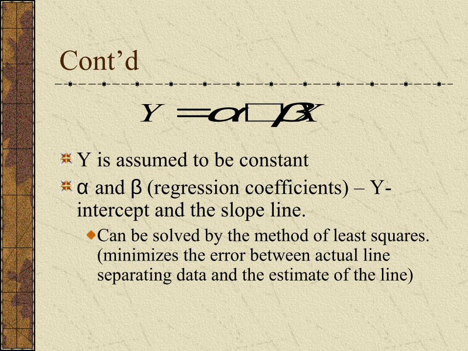
Y is assumed to be constantα and β (regression coefficients) – Y-intercept and the slope line.

Can be solved by the method of least squares. (minimizes the error between actual line separating data and the estimate of the line)

XY βα+=

Cont’d

xy βα −=

( )( )

( )∑=

−

∑=

−==

s

ixix

s

iyiyxix

1

21β

Multiple regression

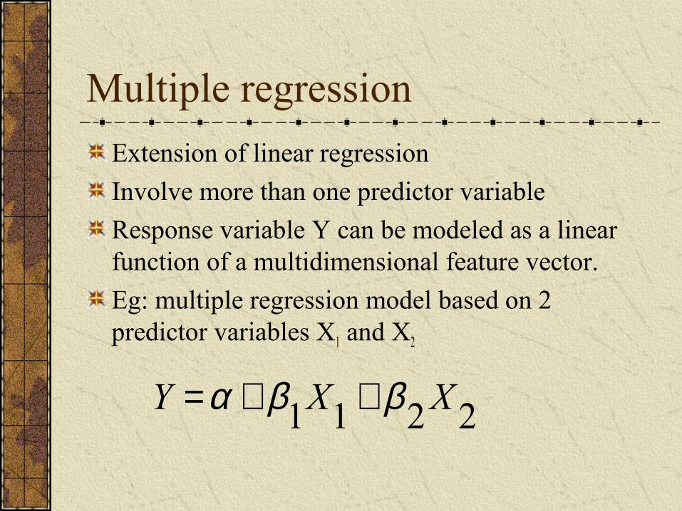
Extension of linear regression

Involve more than one predictor variable

Response variable Y can be modeled as a linear function of a multidimensional feature vector.

Eg: multiple regression model based on 2 predictor variables X1 and X2

2211 XXY ββα ++=

HistogramsA popular data reduction techniqueDivide data into buckets and store average (sum) for each bucketUse binning to approximate data distributionsBucket – horizontal axis, height (area) of bucket – the average frequency of the values represented by the bucketBucket for single attribute-value/frequency pair – singleton bucketsContinuous ranges for the given attribute

Example

A list of prices of commonly sold items (rounded to the nearest dollar)

1,1,5,5,5,5,5,8,8,10,10,10,10,12, 14,14,14,15,15,15,15,15,15,18,18,18,18,18,18,18,18,18,20,20,20,20,20,20,20,21,21,21,21,25,25,25,25,25,28,28,30,30,30.

Refer Fig. 3.9

Cont’d

How are the bucket determined and the attribute values partitioned? (many rules)

Equiwidth, Fig. 3.10

Equidepth

V-Optimal – most accurate & practical

MaxDiff – most accurate & practical

Clustering

Partition data set into clusters, and one can store

cluster representation only

Can be very effective if data is clustered but not if

data is “smeared”/ spread

There are many choices of clustering definitions

and clustering algorithms. We will discuss them

later.

Sampling

Data reduction techniqueA large data set to be represented by much smaller random sample or subset.

4 typesSimple random sampling without replacement (SRSWOR).

Simple random sampling with replacement (SRSWR).

Develop adaptive sampling methods such as cluster sample and stratified sample

Refer Fig. 3.13 pg 131

Discretization and Concept Hierarchy

Discretization reduce the number of values for a given continuous attribute by dividing the range of the attribute into intervals. Interval labels can then be used to replace actual data values

Concept hierarchies reduce the data by collecting and replacing low level concepts (such as numeric values for the attribute age) by higher level concepts (such as young, middle-aged, or senior)

DiscretizationThree types of attributes:

Nominal — values from an unordered setOrdinal — values from an ordered setContinuous — real numbers

Discretization: divide the range of a continuous attribute into intervals because some data mining algorithms only accept categorical attributes.

Some techniques: Binning methods – equal-width, equal-frequencyHistogramEntropy-based methods

Binning

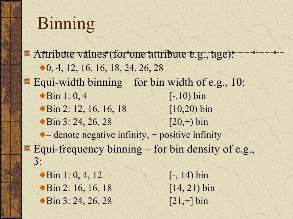
Attribute values (for one attribute e.g., age): 0, 4, 12, 16, 16, 18, 24, 26, 28

Equi-width binning – for bin width of e.g., 10: Bin 1: 0, 4 [-,10) bin Bin 2: 12, 16, 16, 18 [10,20) binBin 3: 24, 26, 28 [20,+) bin– denote negative infinity, + positive infinity

Equi-frequency binning – for bin density of e.g., 3:

Bin 1: 0, 4, 12 [-, 14) binBin 2: 16, 16, 18 [14, 21) binBin 3: 24, 26, 28 [21,+] bin

Summary

Data preparation is a big issue for data mining

Data preparation includes

Data cleaning and data integration

Data reduction and feature selection

Discretization

Many methods have been proposed but still an

active area of research