-­‐1-­‐  

Probing with Severity: Beyond Bayesian Probabilism

and Frequentist Performance

Deborah G Mayo April 8, 2017

Workshop on Probability and Learning

Philosophy Department Columbia University

  -­‐2-­‐  

Brad Efron: “By and large, Statistics is a prosperous and happy country, but it is not a completely peaceful one. Two contending philosophical parties, the Bayesians and the frequentists, have been vying for supremacy over the past two-and-a-half centuries. …Unlike most philosophical arguments, this one has important practical consequences. The two philosophies represent competing visions of how science progresses….” (Efron 2013, p. 130) (empirical Bayesian)

  -­‐3-­‐  

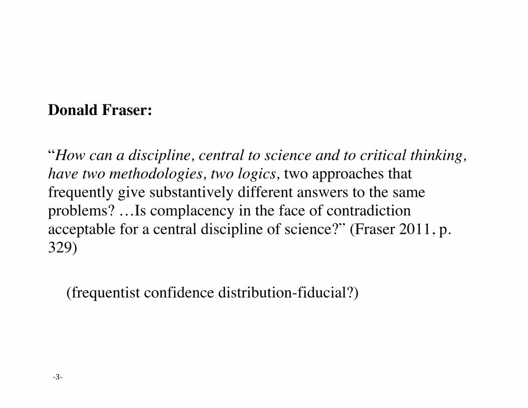
Donald Fraser: “How can a discipline, central to science and to critical thinking, have two methodologies, two logics, two approaches that frequently give substantively different answers to the same problems? …Is complacency in the face of contradiction acceptable for a central discipline of science?” (Fraser 2011, p. 329)

(frequentist confidence distribution-fiducial?)

  -­‐4-­‐  

Jim Berger:

“We [statisticians ] are not blameless….we have not made a concerted professional effort to provide the scientific world with unified testing methodology…and so are tacit accomplices in the unfortunate statistical situation” (J. Berger 2003, p. 4) “…professional agreement on statistical philosophy is not on the immediate horizon, but this should not stop us from agreeing on methodology” (ibid. p. 2)

But what’s methodologically depends on what’s correct philosophically (default Bayesian)

  -­‐5-­‐  

Gelman Gelman & Shalizi “The main point where we disagree with many Bayesians is that we do not think that Bayesian methods are useful for giving the posterior probability that a hypothesis is true.... ... for evaluating a model…”(Gelman & Shalizi 2013, p. 2) “We  see  science–and  applied  statistics–as  resolving  anomalies  via  the  creation  of  improved  models  which  often  includes  their  predecessors  as  special  cases.  This  view  corresponds  closely  to  the  error-­‐statistics  idea  of  Mayo  (1996).”  (Gelman  2011,  p.  70) (Falsificationist Bayes)

  -­‐6-­‐  

Philosophy  of  Statistics  Battles  are  Especially  Important  Now:  Replication  Crisis  

 • Statistical  Findings  Disappear  when  others  look  for  them    

• Beyond  the  social  sciences  to  medicine,  bioinformatics,  genomics  (Big  Data)    

• People  are  serious  about  methodological  reforms  (some  welcome,  others  radical)    

• Need  a  better  understanding  of  statistical,  philosophical,  and  historical  issues  

  -­‐7-­‐  

American Statistical Association: ASA Statement on P-values (2016)

“The statistical community has been deeply concerned about issues of reproducibility and replicability of scientific conclusions. …. much confusion and even doubt about the validity of science is arising. Such doubt can lead to radical choices, such as … to ban p-values (null hypothesis significance testing) Misunderstanding or misuse of statistical inference is only one cause of the “reproducibility crisis” (Peng, 2015), but to our community, it is an important one. (ASA, Wasserstein & Lazar, 2016, p. 129)

  -­‐8-­‐  

In my Commentary on the ASA Doc:

Statistical significance tests are a small part of a rich set of “techniques for systematically appraising and bounding the probabilities…of seriously misleading interpretations of data” (Birnbaum 1970, p. 1033)

These I call error statistical methods (or sampling theory)

  -­‐9-­‐  

Error Statistics

• Statistics: Collection, modeling, drawing inferences from data to claims about aspects of processes

• The inference may be in error

• It’s qualified by a claim about the method’s capabilities to control and alert us to erroneous interpretations (error probabilities)

  -­‐10-­‐  

P-value “p-value. …to test the conformity of the particular data under analysis with H0 in some respect:

…we find a function t = t(y) of the data, to be called the test statistic, such that

• the larger the value of t the more inconsistent are the data with H0;

• The random variable T = t(y) has a (numerically) known probability distribution when H0 is true.…the p-value corresponding to any t as

p = p(t) = P(T ≥ t; H0).” (Mayo and Cox 2006, p. 81)

  -­‐11-­‐  

Testing Reasoning • Clearly, if even larger differences than tobs occur fairly

frequently under H0 (p-value is not small), there’s scarcely evidence of incompatibility with H0

• Small p-value indicates some underlying discrepancy from H0 because very probably you would have obtained a less impressive difference than tobs were H0 true

• This indication isn’t evidence of a genuine statistical effect H, let alone a scientific conclusion H*

Stat-Sub fallacy H => H*

  -­‐12-­‐  

Replication Paradox

Significance Test Critic: It’s much too easy to get a small P-value You: Why do they find it so difficult to replicate the small P-values others found?

Is it easy or is it hard?

  -­‐13-­‐  

• R.A. Fisher: it’s easy to lie with statistics by selective reporting (he called it the “political principle” 1955, p. 75)

• Sufficient finagling—cherry-picking, P-hacking, significance seeking—may practically guarantee a researcher’s preferred claim C gets support, even if it’s unwarranted by evidence

Note: Rejecting a null taken as support for some non-null claim C

  -­‐14-­‐  

Severity Requirement:

• If data x0 agree with a claim C, but the test procedure had little or no capability of finding flaws with C (even if the claim is incorrect), then x0 provide poor evidence for C

Popper: agreement is “too cheap to be worth having” (1983, p. 130)

• Such a test fails a minimal requirement for a stringent or severe test

• My account: severe testing based on error statistics (requires reinterpreting tests)

  -­‐15-­‐  

This alters the role of probability in inference:

typically just two • Probabilism. To assign a degree of probability, confirmation,

support or belief in a hypothesis, given data x0. (e.g., Bayesian, likelihoodist)—with regard for inner coherency

• Performance. Ensure long-run reliability of methods, coverage probabilities (frequentist, behavioristic Neyman-Pearson)

  -­‐16-­‐  

What happened to using probability to assess the error probing capacity by the severity criterion?

• Neither “probabilism” nor “performance” directly captures it.

• Good long-run performance is a necessary, not a sufficient, condition for severity

• That’s why frequentist methods can be shown to have howlers

  -­‐17-­‐  

• Problems with selective reporting, cherry picking, stopping when the data look good, P-hacking, are not problems about long-runs—

• It’s that we cannot say about the case at hand that it has done a good job of avoiding the sources of misinterpreting data (key to revising role of error probabilities)

  -­‐18-­‐  

A claim C is not warranted _______ • Probabilism: unless C is true or probable (gets a probability

boost, is made comparatively firmer)

• Performance: unless it stems from a method with low long-run error.

• Probativism (severe testing) something (a fair amount) has been done to probe ways we can be wrong about C

  -­‐19-­‐  

• If you assume probabilism is required for inference, error

probabilities are relevant for inference only by misinterpretation

• I claim, error probabilities play a crucial role in appraising well-testedness

• It’s crucial to be able to say, C is highly believable or plausible but poorly tested

• Probabilists can allow for the distinct task of severe testing (you may not have to take sides in the stat wars)

  -­‐20-­‐  

• I argue that the central role of probability in statistical inference is severity—its assessment and control.

• Existing error probabilities (confidence levels, significance

levels) may but need not provide severity assessments.

Data x (from test T) are evidence for H only if H has passed a severe test with x (one with a reasonable capability of having detected flaws in H). So we need to assess this “capability” in some way.

  -­‐21-­‐  

By and large today’s handwringing reflects classic foibles

In addition to Stat-Sub fallacy H => H*

“In relation to the test of significance, we may say that a phenomenon is experimentally demonstrable when we know how to conduct an experiment which will rarely fail to give us a statistically significant result” (Fisher 1935, p. 14)

“Isolated” low P-value ≠> H: statistical effect

  -­‐22-­‐  

“Why Most Research Findings are False” Ioannidis

“the high rate of nonreplication (lack of confirmation) of research discoveries is a consequence of the convenient, yet ill-founded strategy of claiming conclusive research findings solely on the basis of a single study assessed by formal statistical significance, typically for a p-value less than 0.05.” (Ioannidis 2005, p. 0696) (Do people really do that? Shame on them.)

• So-called NHST – Null Hypothesis Significance Tests • allows going from statistical to substantive, with a single low P-

value • If defined that way, they exist only as abuses of tests

  -­‐23-­‐  

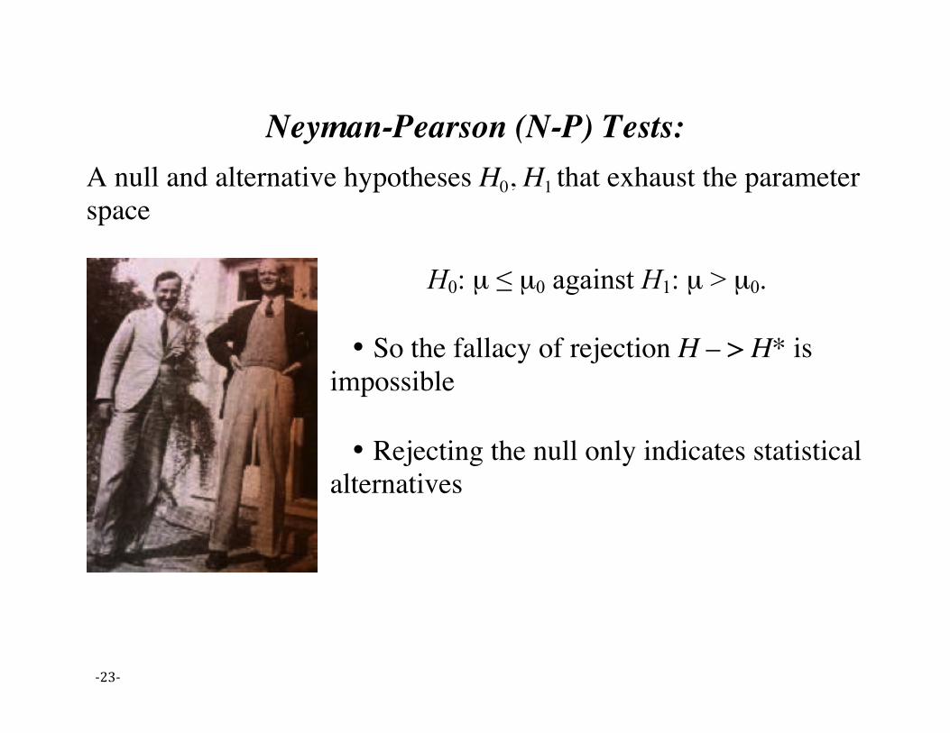
Neyman-Pearson (N-P) Tests:

A null and alternative hypotheses H0, H1 that exhaust the parameter space

H0: µ ≤ µ0 against H1: µ > µ0.

• So the fallacy of rejection H – > H* is

impossible • Rejecting the null only indicates statistical

alternatives

  -­‐24-­‐  

N-P hypothesis test (in their naked mathematical form): maps each x = (x1, …,xn) into either H0, or H1 ensuring the probabilities of erroneous rejections (type I errors) and erroneous acceptances (type II errors) are controlled at small values, e.g., 0.05 or 0.01, the significance level of the test   if d(x0) > cα, "reject" H0, or declare result statistically significant at the α level

if d(x0) < cα, "do not reject" H0, (“accept”) or declare result statistically insignificant at the α level e.g. cα=1.96 for α=.025 The complement of the Type II error = power against μ’ POW(μ’) Pr(d(X) > cα; μ = μ’)

  -­‐25-­‐  

Thought to be limited to “performance” Neyman, not Pearson, was generally the behavioristic-performance one (in theory but not in practice; whereas, Fisher was the reverse) I found an article where Neyman responds to philosopher Carnap’s criticism of “Neyman’s frequentism” Neyman (criticizing Carnap): “I am concerned with the term ‘degree of confirmation’ introduced by Carnap. …We have seen that the application of the locally best one-sided test to the data…failed to reject the hypothesis [that the 26 observations come from a source in which the null hypothesis is true]. The question is: does this result ‘confirm’ the hypothesis that H0 is true of the particular data set?” (Neyman 1955, p. 40-1)

  -­‐26-­‐  

“Locally best one-sided Test T” An IID sample X = (X1, …,Xn) each Xi is Normal N(μ,σ2), σ assumed known; M the sample mean

H0: μ ≤ μ0 against H1: μ > μ0. Test Statistic d(X) = (M – μ0)/σx σx = σ/√𝑛

Test fails to reject the null, d(x0) ≤ cα.

“The question is: does this result ‘confirm’ the hypothesis that [H0 is true of x0)]?” (Neyman 1955, p. 40).

  -­‐27-­‐  

Carnap says yes… Neyman:

“….the attitude described is dangerous. …the chance of detecting the presence [of discrepancy δ from the null], when only [this number] of observations are available, is extremely slim, even if [δ is present].” (Neyman 1955, p. 41) “The situation would have been radically different if the power function…were greater than 0.95.” “A more cautious attitude would be to form one’s intuitive opinion only after studying the power function of the test applied.” (ibid.)

  -­‐28-­‐  

Power  Analysis  

If Pr(d(X) > cα; μ = μ0 + δ) is high d(X) < cα

infer: discrepancy < δ

P(d(X) > cα; μ = μ0 + δ) Power at μ’ μ’ = μ0 + δ Strict behaviorists only use power for planning; Neyman is using it for post-data interpretation. (given it’s continuous, can use ≥ or >)

  -­‐29-­‐  

Severity & Fallacies of Non-Statistically Significant Results  

Neyman’s criticism of Carnap deals with a classic fallacy of non-significant results: to construe such a “negative” result as evidence for the correctness of the null hypothesis.

“no evidence against” is not “evidence for”

Merely surviving the statistical test is too easy, occurs too frequently, even when the null is false.

“… it is a little rash to base one’s intuitive confidence in a given hypothesis on the fact that a test failed to reject this hypothesis.” (Neyman, ibid.)    

  -­‐30-­‐  

Power vs SEV Post Data (1) P(d(X) > cα; μ = μ0 + δ) Power to detect δ

• Neyman requires (1) to be high (for non-significance to warrant μ < μ0 + δ)

• Just missing the cut-off cα is the worst case

• It is more informative to look (2):

(2) P(d(X) > d(x0); μ = μ0 + δ) “attained power”

• can be low while (2) is high

• a measure of the severity for the inference μ < μ0 + δ

  -­‐31-­‐  

Frequentist Principle of Evidence

In Mayo and Cox 2006, it’s in terms of the P-value

FEV: insignificant result: A moderate P-value is evidence of the absence of a discrepancy δ from H0, only if there is a high probability the test would have given a worse fit with H0 (i.e., d(X) > d(x0)) were a discrepancy δ to exist. (pp. 83-4)  (i.e., only if (2) is high)

Assumes the test passes an “audit” (selection effects are taken account of, model assumptions not violated) “Frequentist Statistics as a Theory of Inductive Inference”

  -­‐32-­‐  

Duality with (1 – ε) Upper confidence Bound Test T: Normal testing: H0: μ < μ0 vs H1: μ > μ0 σ is known (FEV/SEV): If d(x) is not statistically significant, then μ < M0 + kεσ /√𝑛 passes test T with severity (1 – ε), where P(d(X) > kε) = ε. (Mayo 1996, Mayo and Spanos 2006, 2011):

  -­‐33-­‐  

If one wants to emphasize the post-data measure, one can write:

SEV(μ < M0 + kσx): The severity with which

(μ < M0 + kσx)

passes test T Severity has 3 terms: SEV(Test, outcome, inference) Significance tests require a SEV supplement to grapple with Principle 5: A p-value does not measure the size of an effect

  -­‐34-­‐  

One can consider a series of upper discrepancy bounds…

SEV(μ < M 0 + 0σx) = .5 SEV(μ < M 0 + .5σx) = .7 SEV(μ < M 0 + 1σx) = .84 SEV(μ < M 0 + 1.5σx) = .93 SEV(μ < M 0 + 1.96σx) = .975

Is this just another way to say how probable each claim is?

  -­‐35-­‐  

No. This would lead to inconsistencies Some call it a “confidence distribution” Probability logic differs from a logic for “how well-tested” (or “corroborated”) a claim is • low severity is not just a little bit of evidence, but bad

evidence, no test • Both C and ~C can be poorly tested

  -­‐36-­‐  

Severity vs. Rubbing–off The severity construal is different from what I call the

Rubbing off construal: The procedure is rarely wrong, therefore, the probability it is wrong in this case is low.

Still too much of a performance criteria, too behavioristic The long-run reliability of the rule is a necessary but not a sufficient condition to infer H (with severity) Today’s fiducialists?

  -­‐37-­‐  

The reasoning instead is counterfactual: H: μ < M0 + 1.96σx

(i.e., μ < CIu )

H passes severely because were this inference false, and the true mean μ > CIu then, very probably, we would have observed a larger sample mean. [1] Examples in handout  

  -­‐38-­‐  

The supplement for rejection avoids fallacies of significant results in an analogous way

• Infer a substantive inference unwarranted from the statistical

inference

• Infer a discrepancy from the null beyond what the test warrants

Severity goes in the opposite direction of power when inferring a discrepancy from the null with a statistically significant result:

An α-significant difference indicates less of a discrepancy from the null with large n than if it resulted from a smaller sample size.

  -­‐39-­‐  

Rather than number crunching, I want to turn to a conceptual issue (It comes up in the ASA document)

  -­‐40-­‐  

ASA Statement: P-values aren’t posteriors in hypotheses

 Principle 2: P-values do not measure (a) the probability that the studied hypothesis is true, or (b) the probability that the data were produced by random chance alone. I inserted the (a), (b) should not be equated to (a).

• A delicate issue

  -­‐41-­‐  

“5 sigma observed effect”  

One of the biggest science events of 2012-13 was the announcement on July 4, 2012 of evidence for the discovery of a Higgs particle based on a “5 sigma observed effect”. With the March 2013 data analysis, the 5 sigma difference grew to 7 sigmas. • The discovery was immediately imbued with controversies

from philosophy of statistics

• I’m an outsider to high energy physics, HEP, a philosopher of statistics should be able to illuminate some of the more public controversies e.g., P-values.

  -­‐42-­‐  

O’Hagan, prompted by Lindley To the ISBA: “Dear Bayesians: We’ve heard a lot about the Higgs boson. ...Specifically, the news referred to a confidence interval with 5-sigma limits.… Five standard deviations, assuming normality, means a p-value of around 0.0000005… Why such an extreme evidence requirement? We know from a Bayesian perspective that this only makes sense if (a) the existence of the Higgs boson has extremely small prior probability and/or (b) the consequences of erroneously announcing its discovery are dire in the extreme. … …. Are the particle physics community completely wedded to frequentist analysis? If so, has anyone tried to explain what bad science that is?”

  -­‐43-­‐  

Bad science?

• HEP physicists are sophisticated with their statistical

methodology: they’d seen too many bumps disappear

• They want to ensure that before announcing the hypothesis H*: “a new particle has been discovered” that:

H* has been given a severe run for its money.

Significance tests and cognate methods (confidence intervals) are methods of choice here for good reason

  -­‐44-­‐  

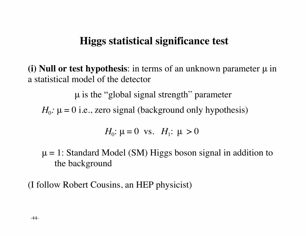
 Higgs statistical significance test (i) Null or test hypothesis: in terms of an unknown parameter μ in a statistical model of the detector

μ is the “global signal strength” parameter H0: μ = 0 i.e., zero signal (background only hypothesis)

H0: μ = 0 vs. H1: μ > 0

μ = 1: Standard Model (SM) Higgs boson signal in addition to

the background (I follow Robert Cousins, an HEP physicist)

  -­‐45-­‐  

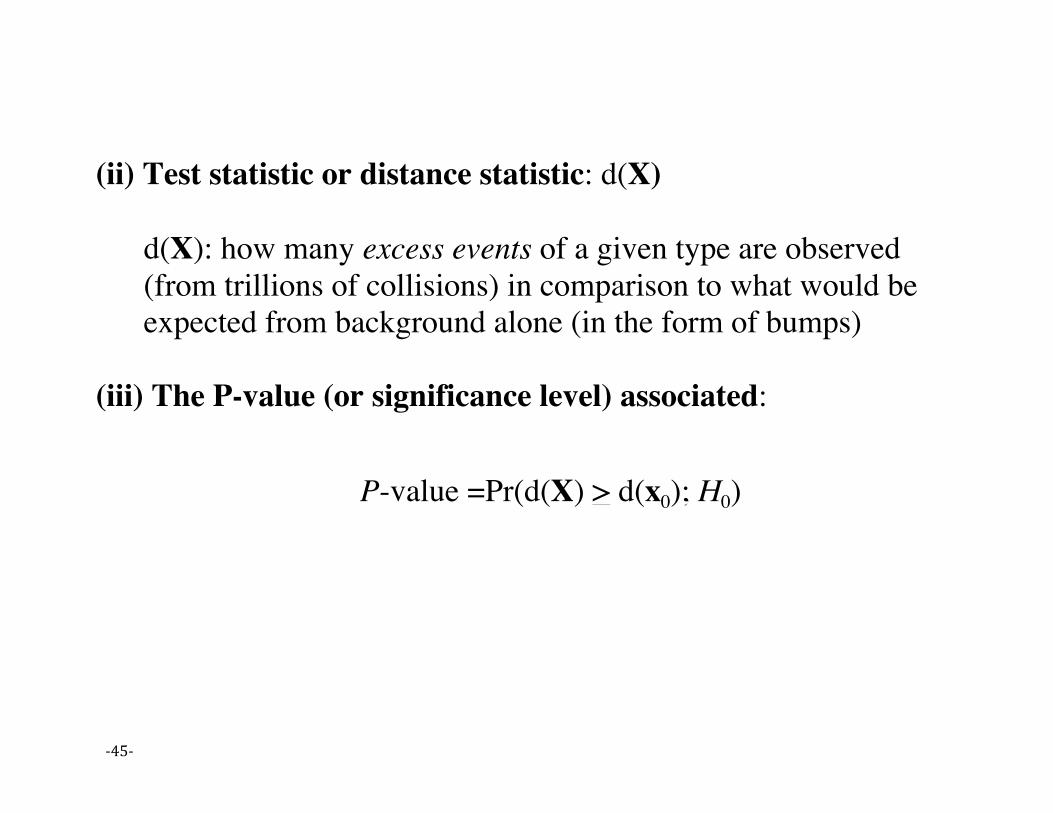
(ii) Test statistic or distance statistic: d(X)  

d(X): how many excess events of a given type are observed (from trillions of collisions) in comparison to what would be expected from background alone (in the form of bumps)

(iii) The P-value (or significance level) associated:

P-value =Pr(d(X) > d(x0); H0)    

  -­‐46-­‐  

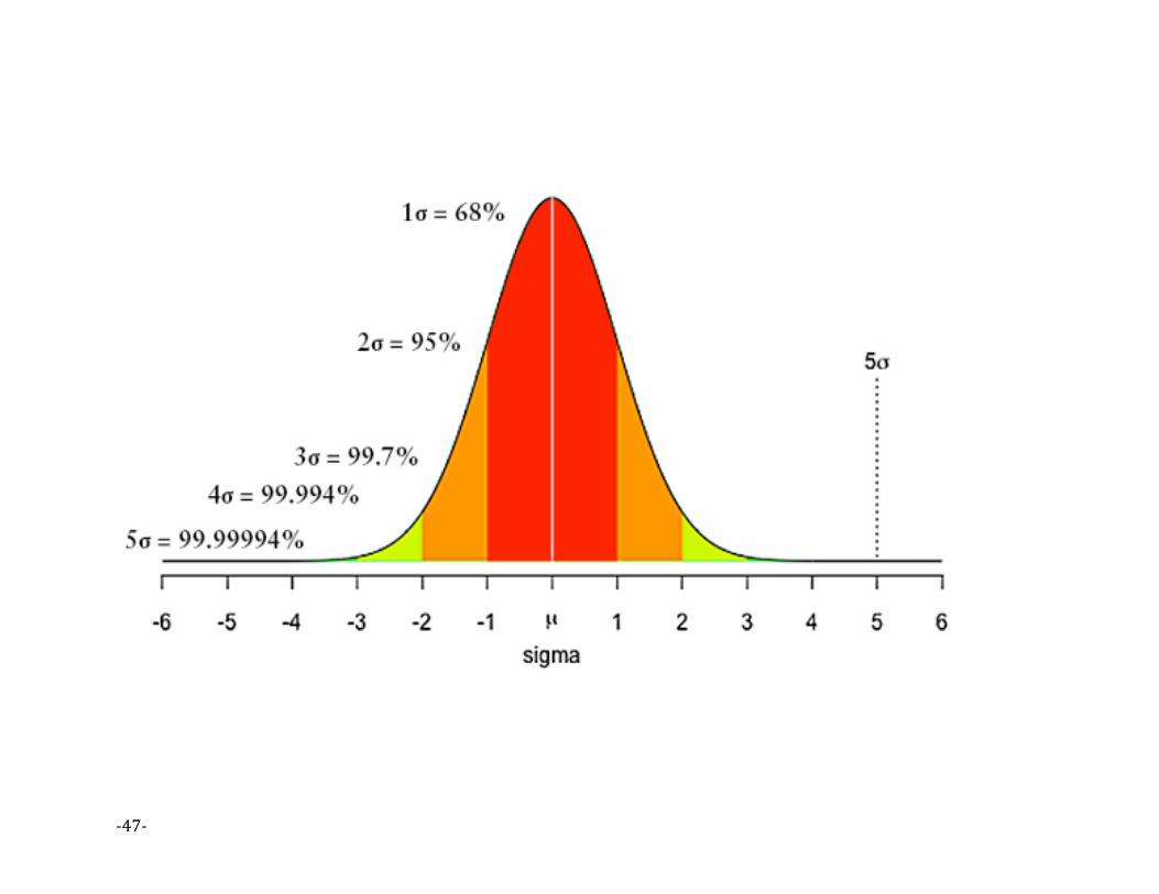
The distribution of statistic d(X) is the sampling distribution

Pr(d(X) > 1; H0) = .16 Pr(d(X) > 2; H0) = .02

Pr(d(X) > 3; H0) = .001 Pr(d(X) > 4; H0) = .00003 Pr(d(X) > 5; H0)= .0000003

The probability of observing results as or more extreme as 5 sigmas, under H0, is approximately 1 in 3,500,000.

  -­‐47-­‐  

 

  -­‐48-­‐  

 There’s generally a rule of interpretation (not strict):

• if d(X) > 5 sigma, infer discovery

• if d(X) > 2 sigma, get more data

They want methods with high capability to detect discrepancies while avoiding mistaking spurious bumps as real.

   

  -­‐49-­‐  

The P-Value Police

When the July 2012 report came out, a number of people set out to grade the different interpretations of the P-value report:

P-value=Pr(d(X) > d(x0); H0) Larry Wasserman calls them the “P-Value Police”.

• Job: to examine if reports by journalists and scientists could be seen to have misinterpreted the sigma levels as posterior probability assignments to the various models and claims.

Sir David Spiegelhalter: Prof of Public Understanding of Risk, Cambridge

  -­‐50-­‐  

Thumbs up or down Thumbs up, to the ATLAS group report:

(i) A statistical combination of these channels and others puts the significance of the signal at 5 sigma, meaning that only one experiment in three million would see an apparent signal this strong in a universe without a Higgs.

Thumbs down to reports such as: (i)’ There is less than a one in 3.5 million chance that their results are a statistical fluctuation (or fluke).

A statistical fluctuation: an apparent signal actually due to chance variability. “the background fluctuation probability” (ATLAS)

  -­‐51-­‐  

Critics allege (i)’misinterprets the P-value as a posterior probability on H0 Not so. H0 does not say the observed results are due to background alone, or are flukes,

H0: μ = 0 If H0 were true (about what’s generating the data), it follows that various results would occur with specified probabilities. (e.g, that large bumps are improbable)

 

  -­‐52-­‐  

What “the results” really are

P-value = Pr(d(X) > d(x0); H0) Pr(overall test procedure would yield d(X) > d(x0); H0)

Recall

“In relation to the test of significance, we may say that a phenomenon is experimentally demonstrable when we know how to conduct an experiment which will rarely fail to give us a statistically significant result” (Fisher 1935, p. 14)

(“isolated” low P-value ≠> H: statistical effect)

  -­‐53-­‐  

Since it’s not just a single result, but an overall test procedure, when you see Pr(d(X) > 5; H0) insert “Test T produces” (1) Pr(Test T produces d(X) > 5; H0) ≤ .0000003

Pr(a 5 sigma fluctuation)

Note: (1) is not a conditional probability (involves a prior)

Pr(Test T produces d(X) > 5 and H0)/ Pr(H0)

Only random variables or their values are conditioned upon. The assignment of probabilities to values of d(X) “under the null” may be seen as a tautologous statement.

  -­‐54-­‐  

Ups C U-1. The probability of the background alone fluctuating up by this amount

or more is about one in three million.

U-2. Only one experiment in three million would see an apparent signal this strong in a universe described in Ho.

U-3. The probability that their signal would result by a chance fluctuation was less than one chance in 3 million

Downs D D-1. The probability their results were due to the background fluctuating up

by this amount or more is about 1 in 3 million.

D-2. One in 3 million is the probability the signal is a false positive—a fluke produced by random statistical fluctuation.

D-3. The probability that their signal was a result of a chance fluctuation was less than one chance in 3 million.

  -­‐55-­‐  

Various  objections  to  “this”  

(i) the P-value refers to a difference as great or greater–a tail area.

Reply: But if the probability {d(X) ≥ d(x)}is low under H0, then Pr(d(X) = d(x);H0) is even lower.

(ii) frequentists don’t assign a probability to this particular data (on July 4, 2012), except maybe 0 or 1.

Reply: True, but that’s the way frequentists always give probabilities to generic events, whether they actual or hypothetical excess of 5 sigma

   

  -­‐56-­‐  

Another Possibility: How it looks to a Bayesian probabilist

“The key distinction between Bayesian and sampling theory statistics is the issue of what is to be regarded as random and what is to be regarded as fixed. To a Bayesian, parameters are random and data, once observed, are fixed” (Kadane 2011, p. 437)

“[t]o a sampling theorist, data are random even after being observed, but parameters are fixed” (ibid.). (violates the Likelihood Principle)

  -­‐57-­‐  

Through a Bayesian probabilist lens…. D-1 through D-3 seem to assign a probability to a hypothesis (about the parameter) since the data are known, only the parameter is unknown. But they’re to be scrutinizing a non-Bayesian procedure.  To an error statistician, the probability that the results are a mere statistical fluctuation = the probability the method would produce results (e.g., bumps) as impressive as these, under H0.    

  -­‐58-­‐  

Not some mysterious reference to “outcomes other than the ones observed”

The error probabilities in U-1 through U-3 are based on simulating relative frequencies of events where H0: μ = 0 (given a detector model) with much cross-checking

(1) Pr(test T would produce a P-value < .0000003; H0) < .0000003.

D-1, 2, 3 are just slightly imprecise ways of expressing U-1,2,3. So what’s the legitimate objection to D-1, 2, 3?

  -­‐59-­‐  

The real problem with D-1 through D-3

It’s the danger in moving from them to their complements: From: There’s a .0000003 probability their results are due to chance, to There’s a .999999 (or whatever) probability their results are not due to chance, are not a fluctuation and so on And those claims are wrong.

  -­‐60-­‐  

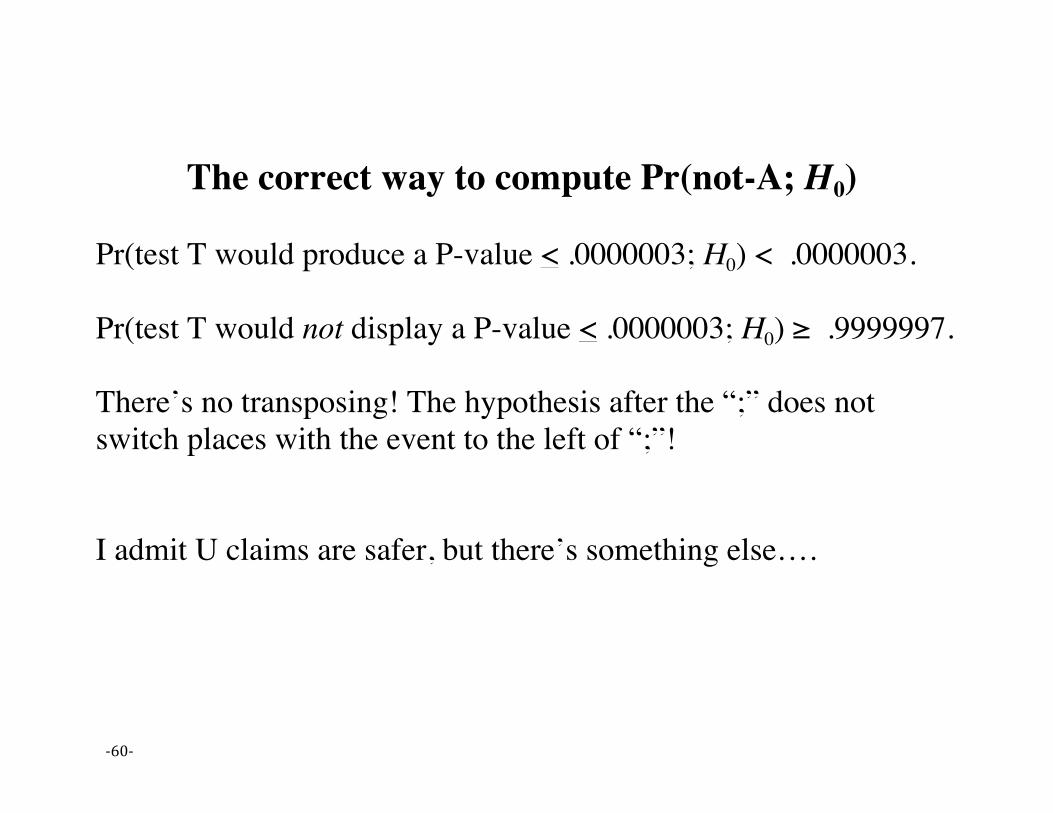
The correct way to compute Pr(not-A; H0)

Pr(test T would produce a P-value < .0000003; H0) < .0000003. Pr(test T would not display a P-value < .0000003; H0) ≥ .9999997. There’s no transposing! The hypothesis after the “;” does not switch places with the event to the left of “;”! I admit U claims are safer, but there’s something else….

  -­‐61-­‐  

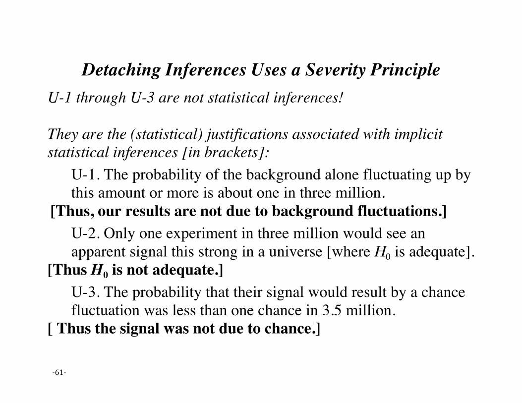
Detaching Inferences Uses a Severity Principle U-1 through U-3 are not statistical inferences! They are the (statistical) justifications associated with implicit statistical inferences [in brackets]:

U-1. The probability of the background alone fluctuating up by this amount or more is about one in three million.

[Thus, our results are not due to background fluctuations.] U-2. Only one experiment in three million would see an apparent signal this strong in a universe [where H0 is adequate].

[Thus H0 is not adequate.] U-3. The probability that their signal would result by a chance fluctuation was less than one chance in 3.5 million.

[ Thus the signal was not due to chance.]

  -­‐62-­‐  

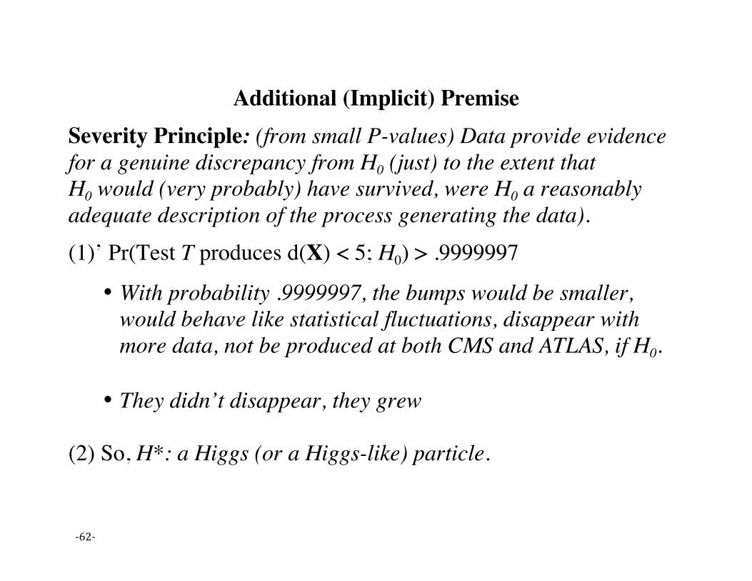
Additional (Implicit) Premise Severity Principle: (from small P-values) Data provide evidence for a genuine discrepancy from H0 (just) to the extent that H0 would (very probably) have survived, were H0 a reasonably adequate description of the process generating the data). (1)’ Pr(Test T produces d(X) < 5; H0) > .9999997

• With probability .9999997, the bumps would be smaller, would behave like statistical fluctuations, disappear with more data, not be produced at both CMS and ATLAS, if H0.

• They didn’t disappear, they grew

(2) So, H*: a Higgs (or a Higgs-like) particle.

  -­‐63-­‐  

What’s detached with high severity?

 

ATLAS reports: “these results provide conclusive evidence for the discovery of a new particle with mass [approximately 125 GeV]” (Atlas Collaboration 2012, p. 15) H*: a Higgs boson consistent with the SM (at the levels of precision and accuracy of these experiments)

 

  -­‐64-­‐  

The inference goes beyond a p-value report Infer:

There is strong evidence for (first) a genuine discrepancy from H0 (later) H*: a Higgs (or a Higgs-like) particle.

Gradations: indication, evidence, discovery (up to July 4, 2012)

  -­‐65-­‐  

Main role for significance tests is: Curb your enthusiasm It affords a standard for:

• denying sufficient evidence of a new particle, inferring “not a genuine effect”, and

• ruling out values of various parameters, e.g., mass ranges.

 

  -­‐66-­‐  

 Look Elsewhere Effect (LEE)

A nominal (or local) P-value: the P-value at a particular, data-determined, mass. But the probability of so impressive a difference anywhere in a mass range would be greater than the local one. Requiring a smaller P-value (i.e., bigger difference), at least 5 sigma, is akin to adjusting for multiple trials or look elsewhere effect LEE.

  -­‐67-­‐  

2015/16 Update When the collider restarted in 2015, it had far greater collider energies than before. On December 15, 2015 something exciting happened: “ATLAS and CMS both reported a small "bump" in their data at a much higher energy level than the Higgs: 750 GeV (compared to 125 GeV). Hundreds of theory papers that attempt to explain the signal” I believe it was 500. The significance reported by CMS is still far below physicists’ threshold for a discovery: 5 sigma, or a chance of around 3 in 10 million that the signal is a statistical fluke. (Castelvecchi & Gibney 2016)

The inference to a genuine discovery didn’t pass severely, and was then falsified

  -­‐68-­‐  

Some HEP may be unhappy with me: Am I encouraging a construal of P-values that physicists have bent over backwards to avoid?

I think they are reacting to critical reports based on how things look from Bayesian probabilists’ eyes. • For a Bayesian, once the data are known, they are fixed

• For the severe tester, Pr{d(X) > d(x0); H} for various H) isn’t

irrelevant once d(x0) is known. It’s the way to determine, with the addition of the severe testing principles, whether the null hypothesis can be falsified  

  -­‐69-­‐  

Concluding Remarks Underlying the debates are two assumptions as to:

What we need Probabilism: the role of probability in inference is to assign a degree of belief, support, confirmation

What we get from error statistical (“frequentist’ )methods

N-P Performance (so irrelevant to inference) A Fisherian attempts to be evidential but p-values aren’t posterior probabilities (so it too fails)

  -­‐70-­‐  

We reject probabilism and performance • Probabilism says H is not justified unless it’s true or probable

(or increases probability, makes firmer).

• Performance says H is not justified unless it stems from a method with low long-run error

• Probativism says H is not justified unless we’ve probed done to probe ways we can be wrong about H, and found them absent

  -­‐71-­‐  

• The severity principle directs us to the relevant error probabilities, avoiding the classic counterintuitive examples

• Where differences remain (disagreement on numbers) e.g., P-values and posteriors, we should recognize the difference in the goals promoted

  -­‐72-­‐  

Thinking we want a posterior probability in H* might be a slip from what may be inferred from this legitimate high probability:

Pr(test T would not reach 5 sigma; H0) > .9999997

With probability .9999997, our methods would show that the bumps disappear, under the assumption data are due to background H0. They don’t disappear but grow. Infer H*

  -­‐73-­‐  

Test T+: Normal testing: H0: μ < μ0 vs. H1: μ > μ0 σ known  

(FEV/SEV): If d(x) is not statistically significant, then μ < M0 + kεσ/√𝑛 passes the test T+ with severity (1 – ε). (FEV/SEV): If d(x) is statistically significant, then μ > M0 – kεσ/√𝑛 passes the test T+ with severity (1 – ε).

where P(d(X) > kε) = ε (standard Normal curve)

  -­‐74-­‐  

FEV: insignificant result: A moderate P-value is evidence of the absence of a discrepancy δ from H0, only if there is a high probability the test would have given a worse fit with H0 (i.e., d(X) > d(x0)) were a discrepancy δ to exist. FEV significant result d(X) > d(x0) is evidence of discrepancy δ from H0, if and only if, there is a high probability the test would have d(X) < d(x0) were a discrepancy as large as δ absent.

  -­‐75-­‐  

Dear Bayesians,

A question from Dennis Lindley prompts me to consult this list in search of answers.

We've heard a lot about the Higgs boson. The news reports say that the LHC needed convincing evidence before they would announce that a particle had been found that looks like (in the sense of having some of the right characteristics of) the elusive Higgs boson. Specifically, the news referred to a confidence interval with 5-sigma limits.

Now this appears to correspond to a frequentist significance test with an extreme significance level. Five standard deviations, assuming normality, means a p-value of around 0.0000005. A number of questions spring to mind.

1. Why such an extreme evidence requirement? We know from a Bayesian perspective that this only makes sense if (a) the existence of the Higgs boson (or some other particle sharing some of its properties) has extremely small prior probability and/or (b) the consequences of erroneously announcing its discovery are dire in the extreme. Neither seems to be the case, so why 5-sigma?

2. Rather than ad hoc justification of a p-value, it is of course better to do a proper Bayesian analysis. Are the particle physics community completely wedded to frequentist analysis? If so, has anyone tried to explain what bad science that is?

3. We know that given enough data it is nearly always possible for a significance test to reject the null hypothesis at arbitrarily low p-values, simply because the parameter will never be exactly equal to its null value. And apparently the LNC has accumulated a very large quantity of data. So could even this extreme p-value be illusory?

If anyone has any answers to these or related questions, I'd be interested to know and will be sure to pass them on to Dennis.

Regards,

Tony

  -­‐76-­‐  

[1] Duality between a 1-sided test and the upper CI bound:  Example: X’s are Normal IID H0: μ ≤ 0 vs H1: μ > 0 n = 100 σ = 2 σ/√100 =.2

Let M0 = .4 (the ~2 SD cut-off) SEV(μ ≤ .8) = Pr(M > .4; μ > .8)

Compute at Pr(M > .4; μ = μ’= .8) since SEV is larger for μ > .8

Test Statistic d*(X) = √100 (M - μ’)/σ

So we get: d*(X) = √100 (.4 – .8)/2 = -.4/.2 = -2 Area to the right of -2 on N(0,1) chart is .975 .8 is the .975 upper confidence bound (we’d estimate σ)

Infer μ ≤ M0 + 2σ/√𝑛

  -­‐77-­‐  

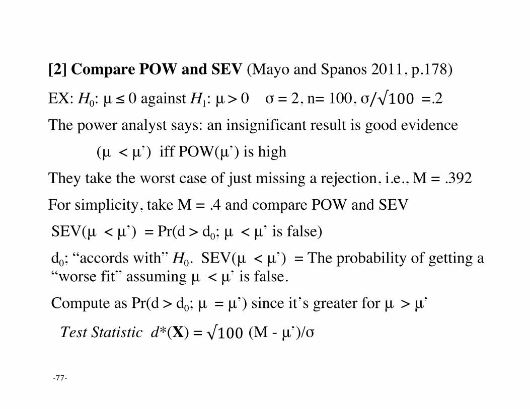
[2] Compare POW and SEV (Mayo and Spanos 2011, p.178)

EX: H0: μ ≤ 0 against H1: μ > 0 σ = 2, n= 100, σ/√100 =.2 The power analyst says: an insignificant result is good evidence

(μ < μ’) iff POW(μ’) is high They take the worst case of just missing a rejection, i.e., M = .392 For simplicity, take M = .4 and compare POW and SEV SEV(μ < μ’) = Pr(d > d0; μ < μ’ is false) d0; “accords with” H0. SEV(μ < μ’) = The probability of getting a “worse fit” assuming μ < μ’ is false. Compute as Pr(d > d0; μ = μ’) since it’s greater for μ > μ’

Test Statistic d*(X) = √100 (M - μ’)/σ

  -­‐78-­‐  

Consider the inference: μ < .2 POW(.2) = Pr (d > .4; .2) = .16 (inference to μ < .2 is always lousy) This is to compute SEV(μ < .2) assuming M = .4 the critical value Compute at Pr(d > d0; μ = .2) since it’s greater for μ > .2 Pr(d > .4; μ’ = .2 )

d*= (.4 - .2)/.2 = 1, so SEV(μ < .2) = .16 SEV takes account of the particular insignificant M0 value: Let M = .3: SEV(μ < .2) = Pr(d > .2; μ = .2)

d*= (.3 – .2)/.2 = .5, so SEV(μ < .2) = .3 Let M = .1: SEV(μ < .2) = Pr(d > .1; μ = .2)

d*= (.1 – .2)/.2 = -.5 so SEV(μ < .2) = .69

  -­‐79-­‐  

The ASA’s Six Principles

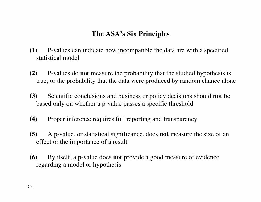
(1) P-values can indicate how incompatible the data are with a specified statistical model

(2) P-values do not measure the probability that the studied hypothesis is true, or the probability that the data were produced by random chance alone

(3) Scientific conclusions and business or policy decisions should not be

based only on whether a p-value passes a specific threshold

(4) Proper inference requires full reporting and transparency

(5) A p-value, or statistical significance, does not measure the size of an effect or the importance of a result

(6) By itself, a p-value does not provide a good measure of evidence

regarding a model or hypothesis    

  -­‐80-­‐  

General References:

Berger, J. O. (2003), “Could Fisher, Jeffreys and Neyman Have Agreed on Testing?” Statistical Science 18(1), 1–12.

Birnbaum, A. (1970). “Statistical Methods in Scientific Inference (letter to the Editor),'”Nature 225(5237): 1033.

Cox, D. R. and Mayo, D. 2010. 'Objectivity and Conditionality in Frequentist Inference', in Mayo and Spanos (eds.), pp. 276–304.

Cousins, R.D. (2017). "The Jeffreys–Lindley paradox and discovery criteria in high energy physics". Synthese 194(2): 395-432.

Efron, B. (2013). “A 250-Year Argument: Belief, Behavior, and the Bootstrap”. Bulletin of the American Mathematical Society 50(1): 126-46.

Fisher, R. A. (1935). The Design of Experiments. Edinburgh: Oliver and Boyd. Fisher, R. A. (1955). “Statistical Methods and Scientific Induction”. Journal of the Royal Statistical

Society, Series B (Methodological) 17(1): 69–78. Fraser, D. A. S. (2011), Is Bayes Posterior just Quick and Dirty Confidence? Rejoinder. Statistical

Science 26(3), 329-331. Gelman, A. (2011). “Induction and Deduction in Bayesian Data Analysis.” In Rationality, Markets

and Morals: Studies at the Intersection of Philosophy and Economics 2, pp. 67-78. Gelman, A., & Shalizi, C. (2013). Philosophy and the Practice of Bayesian Statistics and Rejoinder.

Brit. J. Math. & Stat. Psych. 66(1), 8–38; 76-80.

  -­‐81-­‐  

Ioannidis, J. 2005. “Why most published research findings are false”, PLoS Med 2(8):0696-0701. Kadane, Joseph B. 2011. Principles of Uncertainty. Chapman and Hall/CRC. Mayo, D. G. (1996). Error and the Growth of Experimental Knowledge. Science and Its Conceptual

Foundation. Chicago: University of Chicago Press. Mayo, D. G. (2014). “On the Birnbaum Argument for the Strong Likelihood Principle” (with

discussion), Statistical Science 29(2): 227-39, 261-6. Mayo, D. G. (2016) “Don't Throw Out the Error Control Baby with the Bad Statistics Bathwater: A

Commentary”, “The ASA's Statement on p-Values: Context, Process, and Purpose”, The American Statistician, vol. 70, no. 2, supplemental materials; article 15.) http://www.tandfonline.com/doi/pdf/10.1080/00031305.2016.1154108.

Mayo, D.G. and Cox, D. R. (2006). "Frequentist Statistics as a Theory of Inductive Inference," Optimality: The Second Erich L. Lehmann Symposium (ed. J. Rojo), Lecture Notes-Monograph series, Institute of Mathematical Statistics (IMS), Vol. 49: 77-97. Reprinted in Error and Inference: Recent Exchanges on Experimental Reasoning, Reliability and the Objectivity and Rationality of Science (D Mayo and A. Spanos eds.), Cambridge: CUP: 247-275. ���

Mayo, D. G. and Spanos, A. (2006). "Severe Testing as a Basic Concept in a Neyman-Pearson Philosophy of Induction," British Journal of Philosophy of Science, 57: 323-357.

Mayo,  D.  G  and  Spanos,  A.  2010.  Error  and  Inference:  Recent  Exchanges  on  Experimental  Reasoning,  Reliability,  and  the  Objectivity  and  Rationality  of  Science,  Cambridge:  Cambridge  University  Press.

Mayo, D. G. and Spanos, A. (2011). “Error Statistics”, in Bandyopadhyay, P. and Forster, M. pp.

  -­‐82-­‐  

152–198. Philosophy of Statistics, Vol. 7, Handbook of the Philosophy of Science. The Netherlands: Elsevier.

Neyman, J. (1955). “The Problem of Inductive Inference.” Communications on Pure and Applied Mathematics 8(1), 13–46.

Peng, R. (2015). “The Reproducibility Crisis in Science: A Statistical Counterattack,” Significance 12: 30–32.

Popper, K. (1983). Realism and the Aim of Science.Totowa, NJ: Rowman and Littlefield. Wasserstein, R. and Lazar, N. (2016). “The ASA’s Statement on P-values: Context, Process and

Purpose”, The American Statistician 70(2): 129-133. On-line commentary at: http://www.tandfonline.com/doi/pdf/10.1080/00031305.2016.1154108

Higgs Online links: • Atlas report: http://cds.cern.ch/record/1494183/files/ATLAS-CONF-2012-162.pdf

• Atlas Higgs experiment, public results: https://twiki.cern.ch/twiki/bin/view/AtlasPublic/HiggsPublicResults

• Castelvecchi, D. & Gibney, E. Nature 18 March 2016: http://www.nature.com/news/hints-of-new-lhc-particle-get-slightly-stronger-1.19589

• CMS Higgs experiment, public results:

  -­‐83-­‐  

https://twiki.cern.ch/twiki/bin/view/CMSPublic/PhysicsResultsHIG

O’Hagan, A. (2012) letter:

§ Original letter with responses: http://bayesian.org/forums/news/3648

§ 1st link in a group of discussions of the letter: http://errorstatistics.com/2012/07/11/is-particle-physics-bad-science/

• Overbye, D. (March 15, 2013) 'Chasing the Higgs', New York Times: http://www.nytimes.com/2013/03/05/science/chasing-the-higgs-boson-how-2-teams-of-rivals-at-CERN-searched-for-physics-most-elusive-particle.html?pagewanted=all

 • Spiegelhalter, D. (August 7, 2012) blog, Understanding Uncertainty , “Explaining 5 sigma for

the Higgs: how well did they do?” http://understandinguncertainty.org/explaining-5-sigma-higgs-how-well-did-they-do

• Wasserman, L. 2012. ‘The Higgs Boson and the P-value Police.’ Normal Deviate Blog, post on 7/11/2012. http://normaldeviate.wordpress.com/2012/07/11/the-higgs-boson-and-the-p-value-police/