Embed Size (px)
Citation preview

A Complete Program Design Course(using PseudoCode)
Damian Gordon

PseudoCodeDamian Gordon

Pseudocode
• The first thing we do when designing a program is to decide on a name for the program.

Pseudocode
• The first thing we do when designing a program is to decide on a name for the program.
• Let’s say we want to write a program to calculate interest, a good name for the program would be CalculateInterest.

Pseudocode
• The first thing we do when designing a program is to decide on a name for the program.
• Let’s say we want to write a program to calculate interest, a good name for the program would be CalculateInterest.
• Note the use of CamelCase.

Pseudocode
• The first thing we do when designing a program is to decide on a name for the program.
• Let’s say we want to write a program to calculate interest, a good name for the program would be CalculateInterest.
• Note the use of CamelCase.
Pseudocode
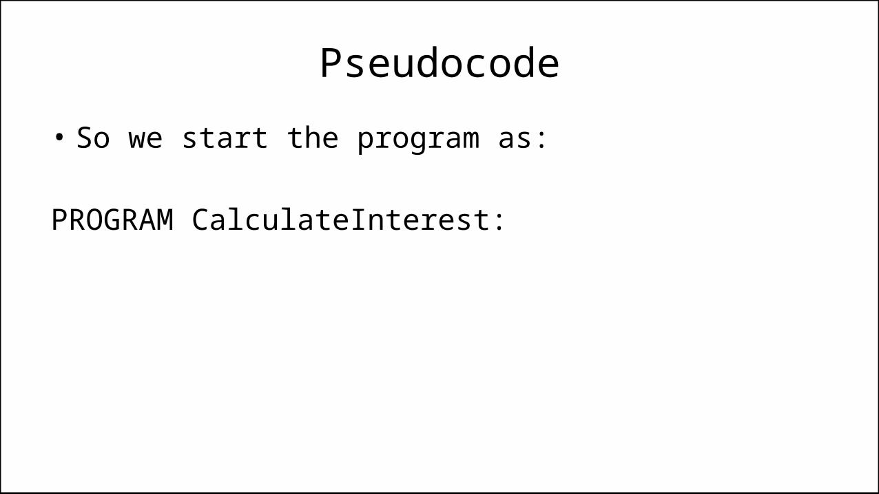
• So we start the program as:
PROGRAM CalculateInterest:

Pseudocode
• So we start the program as:
PROGRAM CalculateInterest:
• And in general it’s:
PROGRAM <ProgramName>:
Pseudocode
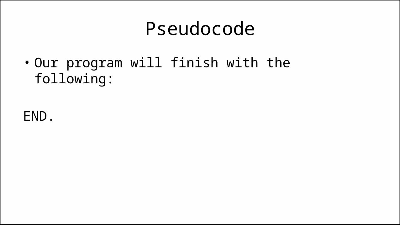
• Our program will finish with the following:
END.

Pseudocode
• Our program will finish with the following:
END.
• And in general it’s the same:
END.
Pseudocode
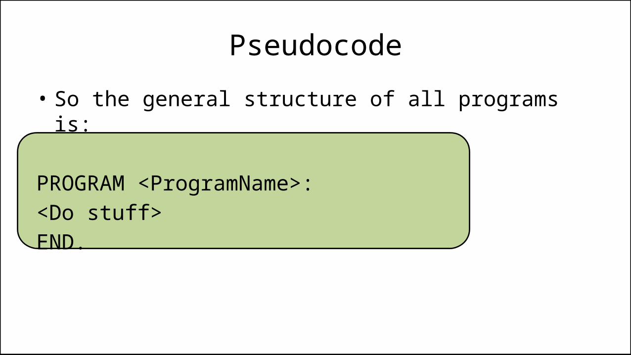
• So the general structure of all programs is:
PROGRAM <ProgramName>:<Do stuff>END.

Components
• Sequence• Selection• Iteration

Top-Down Design
Damian Gordon

Top-Down Design
• Top-Down Design (also known as stepwise design) is breaking down a problem into steps.
• In Top-down Design an overview of the problem is described first, specifying but not detailing any first-level sub-steps.
• Each sub-step is then refined in yet greater detail, sometimes in many additional sub-steps, until the entire specification is reduced to basic elements.

Example
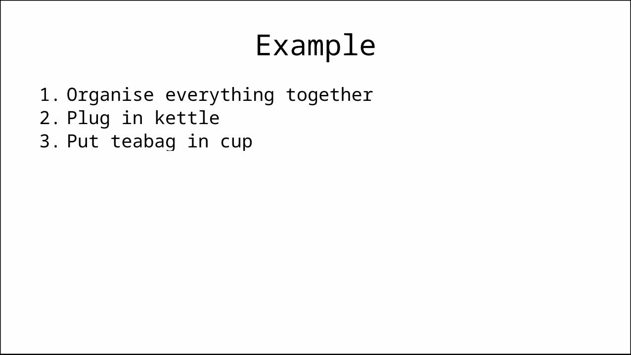
• Making a Cup of Tea

Example
1. Organise everything together2. Plug in kettle3. Put teabag in cup4. Put water into kettle5. Turn on kettle6. Wait for kettle to boil7. Add boiling water to cup8. Remove teabag with spoon/fork9. Add milk and/or sugar10. Serve

Example
1. Organise everything together2. Plug in kettle3. Put teabag in cup4. Put water into kettle5. Turn on kettle6. Wait for kettle to boil7. Add boiling water to cup8. Remove teabag with spoon/fork9. Add milk and/or sugar10. Serve
Example
1. Organise everything together2. Plug in kettle3. Put teabag in cup4. Put water into kettle5. Turn on kettle6. Wait for kettle to boil7. Add boiling water to cup8. Remove teabag with spoon/fork9. Add milk and/or sugar10. Serve

Example
1. Organise everything together2. Plug in kettle3. Put teabag in cup4. Put water into kettle5. Turn on kettle6. Wait for kettle to boil7. Add boiling water to cup8. Remove teabag with spoon/fork9. Add milk and/or sugar10. Serve

Example
1. Organise everything together2. Plug in kettle3. Put teabag in cup4. Put water into kettle5. Turn on kettle6. Wait for kettle to boil7. Add boiling water to cup8. Remove teabag with spoon/fork9. Add milk and/or sugar10. Serve

Example
1. Organise everything together2. Plug in kettle3. Put teabag in cup4. Put water into kettle5. Turn on kettle6. Wait for kettle to boil7. Add boiling water to cup8. Remove teabag with spoon/fork9. Add milk and/or sugar10. Serve

Example
1. Organise everything together2. Plug in kettle3. Put teabag in cup4. Put water into kettle5. Turn on kettle6. Wait for kettle to boil7. Add boiling water to cup8. Remove teabag with spoon/fork9. Add milk and/or sugar10. Serve

Example
1. Organise everything together2. Plug in kettle3. Put teabag in cup4. Put water into kettle5. Turn on kettle6. Wait for kettle to boil7. Add boiling water to cup8. Remove teabag with spoon/fork9. Add milk and/or sugar10. Serve

Example
1. Organise everything together2. Plug in kettle3. Put teabag in cup4. Put water into kettle5. Turn on kettle6. Wait for kettle to boil7. Add boiling water to cup8. Remove teabag with spoon/fork9. Add milk and/or sugar10. Serve

Example
1. Organise everything together2. Plug in kettle3. Put teabag in cup4. Put water into kettle5. Turn on kettle6. Wait for kettle to boil7. Add boiling water to cup8. Remove teabag with spoon/fork9. Add milk and/or sugar10. Serve

Example : Step-wise Refinement
Step-wise refinement of step 1 (Organise everything together)1.1 Get a cup1.2 Get tea bags1.3 Get sugar1.4 Get milk1.5 Get spoon/fork.

Example : Step-wise Refinement
Step-wise refinement of step 2 (Plug in kettle)2.1 Locate plug of kettle2.2 Insert plug into electrical outlet

Example : Step-wise Refinement
Step-wise refinement of step 3 (Put teabag in cup)3.1 Take teabag from box3.2 Put it into cup

Example : Step-wise Refinement
Step-wise refinement of step 4 (Put water into kettle)4.1 Bring kettle to tap4.2 Put kettle under water4.3 Turn on tap4.4 Wait for kettle to be full4.5 Turn off tap

Example : Step-wise Refinement
Step-wise refinement of step 5 (Turn on kettle)5.1 Depress switch on kettle

Over to you…

SequenceDamian Gordon

Pseudocode
• When we write programs, we assume that the computer executes the program starting at the beginning and working its way to the end.
• This is a basic assumption of all algorithm design.

Pseudocode
• When we write programs, we assume that the computer executes the program starting at the beginning and working its way to the end.
• This is a basic assumption of all algorithm design.• We call this SEQUENCE.

Pseudocode
• In Pseudo code it looks like this:
Statement1;Statement2;Statement3;Statement4;Statement5;Statement6;Statement7;Statement8;

Pseudocode• For example, for making a cup of tea:
Organise everything together;Plug in kettle;Put teabag in cup;Put water into kettle;Wait for kettle to boil;Add water to cup;Remove teabag with spoon/fork;Add milk and/or sugar;Serve;
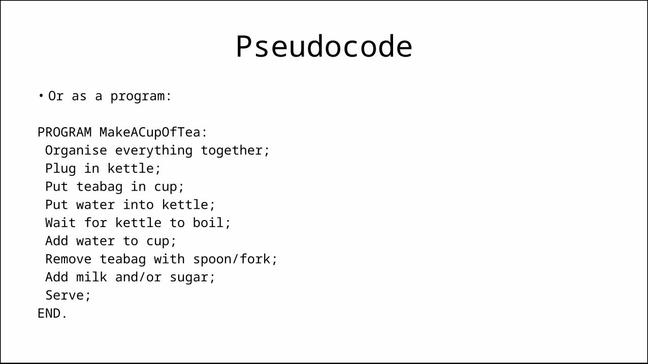
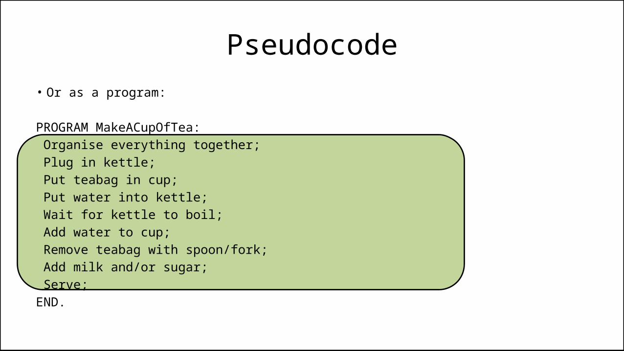
Pseudocode• Or as a program:
PROGRAM MakeACupOfTea: Organise everything together; Plug in kettle; Put teabag in cup; Put water into kettle; Wait for kettle to boil; Add water to cup; Remove teabag with spoon/fork; Add milk and/or sugar; Serve;END.
Pseudocode• Or as a program:
PROGRAM MakeACupOfTea: Organise everything together; Plug in kettle; Put teabag in cup; Put water into kettle; Wait for kettle to boil; Add water to cup; Remove teabag with spoon/fork; Add milk and/or sugar; Serve;END.

Organise everything together
Plug in kettle
Put teabag in cup
Put water into kettle
Turn on kettle
Wait for kettle to boil
Add boiling water to cup
Remove teabag with spoon/fork
Add milk and/or sugar
Serve

Organise everything together
Plug in kettle
Put teabag in cup
Put water into kettle
Turn on kettle
Wait for kettle to boil
Add boiling water to cup
Remove teabag with spoon/fork
Add milk and/or sugar
Serve
START
END

Pseudocode
• So let’s say we want to express the following algorithm:– Read in a number and print it out.

Pseudocode
PROGRAM PrintNumber: Read number; Print out number;END.

Pseudocode
• So let’s say we want to express the following algorithm:– Read in a number and print it out double the number.

Pseudocode
PROGRAM PrintDoubleNumber: Read number; Print 2 * number;END.

VariablesDamian Gordon
Variables
• We know what a variable is from maths.• We’ve all seen this sort of thing in algebra:
2x – 10 = 02x = 10
X = 5
Variables
• We know what a variable is from maths.• We’ve all seen this sort of thing in algebra:
2x – 10 = 02x = 10
X = 5

Variables
• We know what a variable is from maths.• We’ve all seen this sort of thing in algebra:
2x – 10 = 02x = 10
X = 5

Variables
• We know what a variable is from maths.• We’ve all seen this sort of thing in algebra:
2x – 10 = 02x = 10
X = 5

Variables
• We know what a variable is from maths.• We’ve all seen this sort of thing in algebra:
2x – 10 = 02x = 10
X = 5

Variables
• …and in another problem we might have:
3x + 12 = 03x = -12X = -4

Variables
• So a variable contains a value, and that value changes over time.

Variables
• …like your bank balance!

Variables
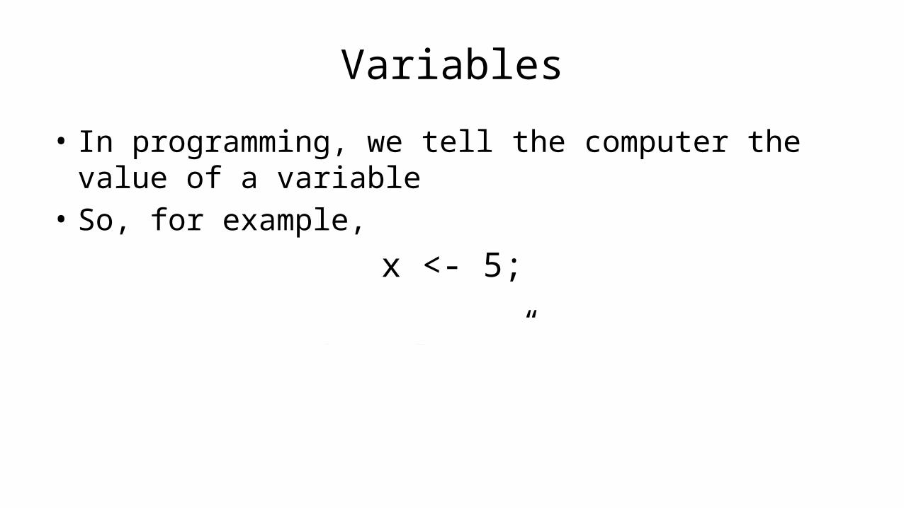
• In programming, we tell the computer the value of a variable• So, for example,
x <- 5
means “X gets the value 5” or “X is assigned 5”
Variables
• In programming, we tell the computer the value of a variable• So, for example,
x <- 5;
means “X gets the value 5” or “X is assigned 5”

Variables
• In programming, we tell the computer the value of a variable• So, for example,
x <- 5;
means “X gets the value 5” or “X is assigned 5”
X

Variables
• In programming, we tell the computer the value of a variable• So, for example,
x <- 5;
means “X gets the value 5” or “X is assigned 5”
X
5

Variables
• And later we can say something like:
x <- 8;
means “X gets the value 8” or “X is assigned 8”

Variables
• If we want to add one to a variable:
x <- x + 1;
means “increment X” or “X is incremented by 1”
X(new)
5X(old)
4+1

Variables
• We can create a new variable Y
y <- x;
means “Y gets the value of X” or “Y is assigned the value of X”
Y
X6
6

Variables
• We can also say:
y <- x + 1;
means “Y gets the value of x plus 1” or “Y is assigned the value of x plus 1”
Y
X6
7
+1

Variables
• All of these variables are integers• They are all whole numbers

Variables
• Let’s look at numbers with decimal points:
P <- 3.14159;
means “p gets the value of 3.14159” or “p is assigned the value of 3.14159”

Variables
• We should really give this a better name:
Pi <- 3.14159;
means “Pi gets the value of 3.14159” or “Pi is assigned the value of 3.14159”

Variables
• We can also have single character variables:
Vitamin <- ‘B’;
means “Vitamin gets the value of B” or “Vitamin is assigned the value of B”

Variables
• We can also have single character variables:
RoomNumber <- ‘2’;
means “RoomNumber gets the value of 2” or “RoomNumber is assigned the value of 2”

Variables
• We can also have a string of characters:
Pet <- “Dog”;
means “Pet gets the value of Dog” or “Pet is assigned the value of Dog”

Variables
• We also have a special type, called BOOLEAN• It has only two values, TRUE or FALSE
IsWeekend <- FALSE;
means “IsWeekend gets the value of FALSE” or “IsWeekend is assigned the value of FALSE”

Pseudocode
• So let’s say we want to express the following algorithm:– Read in a number and print it out.

Pseudocode
PROGRAM PrintNumber: Read Value; Print Value;END.

Pseudocode
• So let’s say we want to express the following algorithm:– Read in a number and print it out double the number.

Pseudocode
PROGRAM PrintDoubleNumber: Read Value; DoubleValue <- 2*Value; Print DoubleValue;END.

Converting Temperatures
• How do we convert from Celsius to Fahrenheit?
• F = (C * 2) + 30
• So if C=25• F = (25*2)+30 = 50+30 = 80

Converting Temperatures
PROGRAM ConvertFromCelsiusToFahrenheit: Print “Please Input Your Temperature in Celsius:”; Read Temp; Print “That Temperature in Fahrenheit:”; Print (Temp*2) + 30;END.

Converting Temperatures
• How do we convert from Fahrenheit to Celsius?
• C = (F -30) / 2
• So if F=80• F = (80-30)/2 = 50/2 = 25

Converting Temperatures
PROGRAM ConvertFromFahrenheitToCelsius: Print “Please Input Your Temperature in Fahrenheit:”; Read Temp; Print “That Temperature in Celsius:”; Print (Temp-30)/2;END.

Selection:IF Statement
Damian Gordon

adsdfsdsdsfsdfsdsdlkmfsdfmsdlkfsdmkfsldfmsk
dddfsdsdfsd

Do you wish to print a receipt?
< YES NO >

Do you wish to print a receipt?
< YES NO >
In the interests of preserving the environment, we prefer not to print a
receipt, but if you want to be a jerk, go ahead.
< PRINT RECEIPT CONTINUE >

Selection
• What if we want to make a choice, for example, do we want to add sugar or not to the tea?

Selection
• What if we want to make a choice, for example, do we want to add sugar or not to the tea?
• We call this SELECTION.

IF Statement
• So, we could state this as:
IF (sugar is required) THEN add sugar; ELSE don’t add sugar;ENDIF;

IF Statement• Adding a selection statement in the program:
PROGRAM MakeACupOfTea: Organise everything together; Plug in kettle; Put teabag in cup; Put water into kettle; Wait for kettle to boil; Add water to cup; Remove teabag with spoon/fork; Add milk; IF (sugar is required) THEN add sugar; ELSE do nothing; ENDIF; Serve;END.

IF Statement
• Or, in general:
IF (<CONDITION>) THEN <Statements>; ELSE <Statements>;ENDIF;

IF Statement
• Or to check which number is biggest:
IF (A > B) THEN Print A; ELSE Print B;ENDIF;

Pseudocode
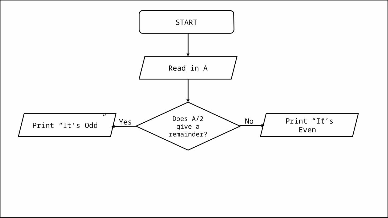
• So let’s say we want to express the following algorithm:– Read in a number, check if it is odd or even.

Pseudocode
PROGRAM IsOddOrEven: Read A; IF (A/2 gives a remainder) THEN Print “It’s Odd”; ELSE Print “It’s Even”; ENDIF;END.

Pseudocode
• We can skip the ELSE part if there is nothing to do in the ELSE part.
• So:IF (sugar is required) THEN add sugar; ELSE don’t add sugar;ENDIF;

Pseudocode
• Becomes:
IF (sugar is required) THEN add sugar;ENDIF;

START

START
Read in A

START
Does A/2 give a remainder?
Read in A

START
Does A/2 give a remainder?
Read in A
YesPrint “It’s Odd”
START
Does A/2 give a remainder?
No
Read in A
YesPrint “It’s Odd” Print “It’s Even”

START
END
Does A/2 give a remainder?
No
Read in A
YesPrint “It’s Odd” Print “It’s Even”

Pseudocode
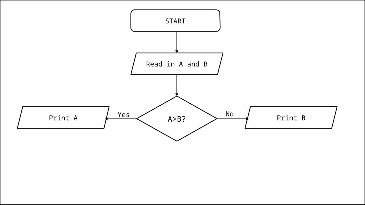
• So let’s say we want to express the following algorithm to print out the bigger of two numbers:– Read in two numbers, call them A and B. Is A is bigger than B, print out A,
otherwise print out B.

Pseudocode
PROGRAM PrintBiggerOfTwo: Read A; Read B; IF (A>B) THEN Print A; ELSE Print B; ENDIF;END.

START

START
Read in A and B

START
A>B?
Read in A and B

START
A>B?
Read in A and B
YesPrint A
START
A>B?No
Read in A and B
YesPrint A Print B

START
END
A>B?No
Read in A and B
YesPrint A Print B

Pseudocode
• So let’s say we want to express the following algorithm to print out the bigger of three numbers:– Read in three numbers, call them A, B and C.
• If A is bigger than B, then if A is bigger than C, print out A, otherwise print out C. • If B is bigger than A, then if B is bigger than C, print out B, otherwise print out C.

PseudocodePROGRAM BiggerOfThree: Read A; Read B; Read C; IF (A>B) THEN IF (A>C) THEN Print A; ELSE Print C; ENDIF; ELSE IF (B>C) THEN Print B; ELSE Print C; ENDIF; ENDIF;END.

START

START
Read in A, B and C

START
A>B?
Read in A, B and C

START
A>B?
Read in A, B and C
YesA>C?

START
A>B?No
Read in A, B and C
YesA>C? B>C?

START
A>B?No
Read in A, B and C
YesA>C? B>C?
Print C
NoNo

START
A>B?No
Read in A, B and C
YesA>C? B>C?
Print A Print C
Yes
NoNo

START
A>B?No
Read in A, B and C
YesA>C? B>C?
Print A Print C Print B
Yes Yes
NoNo

START
END
A>B?
No
Read in A, B and C
YesA>C? B>C?
Print A Print C Print B
Yes Yes
No
No

Selection:CASE Statement
Damian Gordon

Selection
• As well as the IF Statement, another form of SELECTION is the CASE statement.

CASE Statement
• If we had a multi-choice question:

CASE Statement
• If we had a multi-choice question:

CASE StatementRead Answer; IF (Answer == ‘A’) THEN Print “That is incorrect”; ELSE IF (Answer == ‘B’) THEN Print “That is incorrect”; ELSE IF (Answer == ‘C’) THEN Print “That is Correct”; ELSE IF (Answer == ‘D’) THEN Print “That is incorrect”; ELSE Print “Bad Option”; END IF; END IF; END IF; END IF;

CASE StatementPROGRAM MultiChoiceQuestion: Read Answer; IF (Answer == ‘A’) THEN Print “That is incorrect”; ELSE IF (Answer == ‘B’) THEN Print “That is incorrect”; ELSE IF (Answer == ‘C’) THEN Print “That is Correct”; ELSE IF (Answer == ‘D’) THEN Print “That is incorrect”; ELSE Print “Bad Option”; ENDIF; ENDIF; ENDIF; ENDIF;END.

CASE Statement
Read Answer;CASE OF Answer ‘A’ :Print “That is incorrect”; ‘B’ :Print “That is incorrect”; ‘C’ :Print “That is Correct”; ‘D’ :Print “That is incorrect”; OTHER:Print “Bad Option”;ENDCASE;

CASE Statement
PROGRAM MultiChoiceQuestion: Read Answer; CASE OF Answer ‘A’ :Print “That is incorrect”; ‘B’ :Print “That is incorrect”; ‘C’ :Print “That is Correct”; ‘D’ :Print “That is incorrect”; OTHER:Print “Bad Option”; ENDCASE;END.

CASE Statement
• Or, in general:
CASE OF Value Option1: <Statements>; Option2: <Statements>; Option3: <Statements>; Option4: <Statements>; OTHER : <Statements>;ENDCASE;

START
END
Option1
No
Read in A
YesPrint “Option 1”
Option2
No
YesPrint “Option 2”
OTHER
No
YesPrint “OTHER”

CASE Statement
Read Result;CASE OF Result Result => 70 :Print “You got a first”; Result => 60 :Print “You got a 2.1”; Result => 50 :Print “You got a 2.2”; Result => 40 :Print “You got a 3”; OTHER :Print “Dude, you failed”;ENDCASE;

CASE Statement
PROGRAM GetGrade: Read Result; CASE OF Result Result => 70 :Print “You got a first”; Result => 60 :Print “You got a 2.1”; Result => 50 :Print “You got a 2.2”; Result => 40 :Print “You got a 3”; OTHER :Print “Dude, you failed”; ENDCASE;END.

Iteration:WHILE LoopDamian Gordon

WHILE Loop
• Consider the problem of searching for an entry in a phone book with only SELECTION:

WHILE Loop
Get first entry;IF (this is the correct entry) THEN write down phone number; ELSE get next entry; IF (this is the correct entry)
THEN write done entry; ELSE get next entry;
IF (this is the correct entry)……………

WHILE Loop
• We may rewrite this using a WHILE Loop:

WHILE Loop
Get first entry;Call this entry N;WHILE (N is NOT the required entry) DO Get next entry; Call this entry N;
ENDWHILE;

WHILE Loop
PROGRAM SearchForEntry: Get first entry; Call this entry N; WHILE (N is NOT the required entry) DO Get next entry; Call this entry N;
ENDWHILE;END.

WHILE Loop
• Or, in general:
WHILE (<CONDITION>) DO <Statements>;ENDWHILE;

WHILE Loop
• So let’s say we want to express the following algorithm:– Print out the numbers from 1 to 5

WHILE Loop
PROGRAM Print1to5: A <- 1; WHILE (A != 6) DO Print A; A <- A + 1; ENDWHILE;END.

WHILE Loop
START
END
Is A==6?No
A = 1
Yes
Print A
A = A + 1

WHILE Loop
• So let’s say we want to express the following algorithm:– Add up the numbers 1 to 5 and print out the result

WHILE Loop
PROGRAM PrintSum1to5: Total <- 0; A <- 1; WHILE (A != 6) DO Total <- Total + A; A <- A + 1; ENDWHILE; Print Total;END.

WHILE Loop
• So let’s say we want to express the following algorithm:– Calculate the factorial of any value

WHILE Loop
• So let’s say we want to express the following algorithm:– Calculate the factorial of any value– Remember:– 5! = 5*4*3*2*1
– 7! = 7*6 *5*4*3*2*1
– N! = N*(N-1)*(N-2)*…*2*1

WHILE Loop
PROGRAM Factorial: Get Value; Total <- Value - 1; WHILE (Value != 0) DO Total <- Value * Total; Value <- Value - 1; ENDWHILE; Print Total;END.

Iteration:FOR, DO, LOOP Loop
Damian Gordon

FOR Loop
• The FOR loop does the same thing as a WHILE loop but is easier if you are using the loop to do a countdown (or countup).

FOR Loop
• For example:

WHILE Loop
PROGRAM Print1to5: A <- 1; WHILE (A != 6) DO Print A; A <- A + 1; ENDWHILE;END.

FOR Loop
• Can be expressed as:

FOR Loop
PROGRAM Print1to5: FOR A IN 1 TO 5 DO Print A; ENDFOR;END.

FOR Loop
• Or, in general:
FOR Variable IN Range DO <Statements>;ENDFOR;
DO Loop
• The WHILE loop can execute any number of times, including zero times.
• If we are writing a program, and we know that the loop we are using will be executed at least once, we could consider using a DO loop instead.

DO Loop
PROGRAM MenuOptions: DO Print “****** MENU OPTIONS ******”; Print “1) Input Data”; Print “2) Delete Data”; Print “3) Print Report”; Print “9) Exit”; Get Value; WHILE (Value != 9)END.

DO Loop
• Or, in general:
DO <Statements>;WHILE (<Condition>)

LOOP Loop
• The LOOP loop is one that has no condition, so it is an infinite loop. But it does include an EXIT command to break out of the loop if needed.

LOOP Loop
PROGRAM Print1to5: A <- 1; LOOP Print A; IF (A = 6) THEN EXIT; ENDIF; A <- A + 1; ENDLOOP;END.

LOOP Loop
• Or, in general:
LOOP <Statements>; IF (<Condition>) THEN EXIT; ENDIF; <Statements>;ENDLOOP;

Prime NumbersDamian Gordon

Prime Numbers
• So let’s say we want to express the following algorithm:– Read in a number and check if it’s a prime number.

Prime Numbers
• So let’s say we want to express the following algorithm:– Read in a number and check if it’s a prime number.– What’s a prime number?

Prime Numbers
• So let’s say we want to express the following algorithm:– Read in a number and check if it’s a prime number.– What’s a prime number?– A number that’s only divisible by itself and 1, e.g. 7.

Prime Numbers
• So let’s say we want to express the following algorithm:– Read in a number and check if it’s a prime number.– What’s a prime number?– A number that’s only divisible by itself and 1, e.g. 7. – Or to put it another way, every number other than itself and 1 gives a remainder, e.g. For
7, if 6, 5, 4, 3, and 2 give a remainder then 7 is prime.

Prime Numbers
• So let’s say we want to express the following algorithm:– Read in a number and check if it’s a prime number.– What’s a prime number?– A number that’s only divisible by itself and 1, e.g. 7. – Or to put it another way, every number other than itself and 1 gives a remainder, e.g. For
7, if 6, 5, 4, 3, and 2 give a remainder then 7 is prime.– So all we need to do is divide 7 by all numbers less than it but greater than one, and if
any of them have no remainder, we know it’s not prime.

Prime Numbers
• So, • If the number is 7, as long as 6, 5, 4, 3, and 2 give a
remainder, 7 is prime.• If the number is 9, we know that 8, 7, 6, 5, and 4, all give
remainders, but 3 does not give a remainder, it goes evenly into 9 so we can say 9 is not prime

Prime Numbers
• So remember, – if the number is 7, as long as 6, 5, 4, 3, and 2 give a remainder,
7 is prime.• So, in general, – if the number is A, as long as A-1, A-2, A-3, A-4, ... 2 give a
remainder, A is prime.

Prime Numbers
• First Draft:PROGRAM CheckPrime: READ A; B <- A-1; WHILE (B != 1) DO {KEEP CHECKING IF A/B DIVIDES EVENLY} ENDWHILE;
IF (ANY TIME THE DIVISION WAS EVEN) THEN Print “It is not prime”; ELSE Print “It is prime”; ENDIF;END.

Prime NumbersPROGRAM CheckPrime: Read A; B <- A - 1; IsPrime <- TRUE; WHILE (B != 1) DO IF (A/B gives no remainder) THEN IsPrime <- FALSE; ENDIF; B <- B – 1; ENDWHILE; IF (IsPrime = FALSE) THEN Print “Not Prime”; ELSE Print “Prime”; ENDIF;END.

Fibonacci NumbersDamian Gordon

Leonardo Bonacci (aka Fibonacci)
• Born 1170ad• Born in Pisa, Italy• Died 1250ad• An Italian mathematician, considered to
be "the most talented Western mathematician of the Middle Ages".
• Introduced the sequence of Fibonacci numbers which he used as an example in Liber Abaci.
Fibonacci Numbers
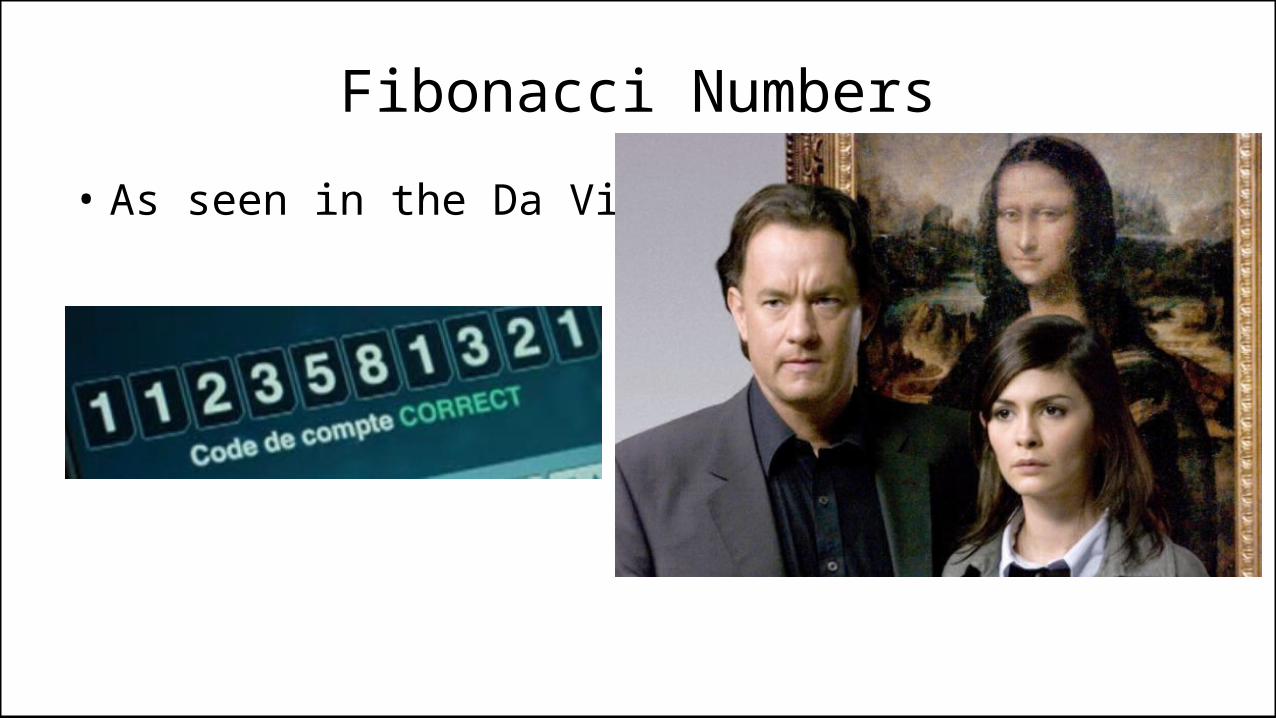
• As seen in the Da Vinci Code:

Fibonacci Numbers
• The Fibonacci numbers are numbers where the next number in the sequence is the sum of the previous two.
• The sequence starts with 1, 1,• And then it’s 2• Then 3• Then 5• Then 8• Then 13

Fibonacci Numbers
PROGRAM FibonacciNumbers: READ A; FirstNum <- 1; SecondNum <- 1; WHILE (A != 2) DO Total <- SecondNum + FirstNum; FirstNum <- SecondNum; SecondNum <- Total; A <- A – 1; ENDWHILE; Print Total;END.

CompressionDamian Gordon

• Rather than have to store every character in a file (e.g. an MP3 file), it would be great if we could find a way of reducing the length of the file to allow it to be stored in a smaller space.
Data Compression

• Also Rather than have to send every character in a message, it would be great if we could find a way of reducing the length of the message to allow it to be transmitted quicker.
Data Compression
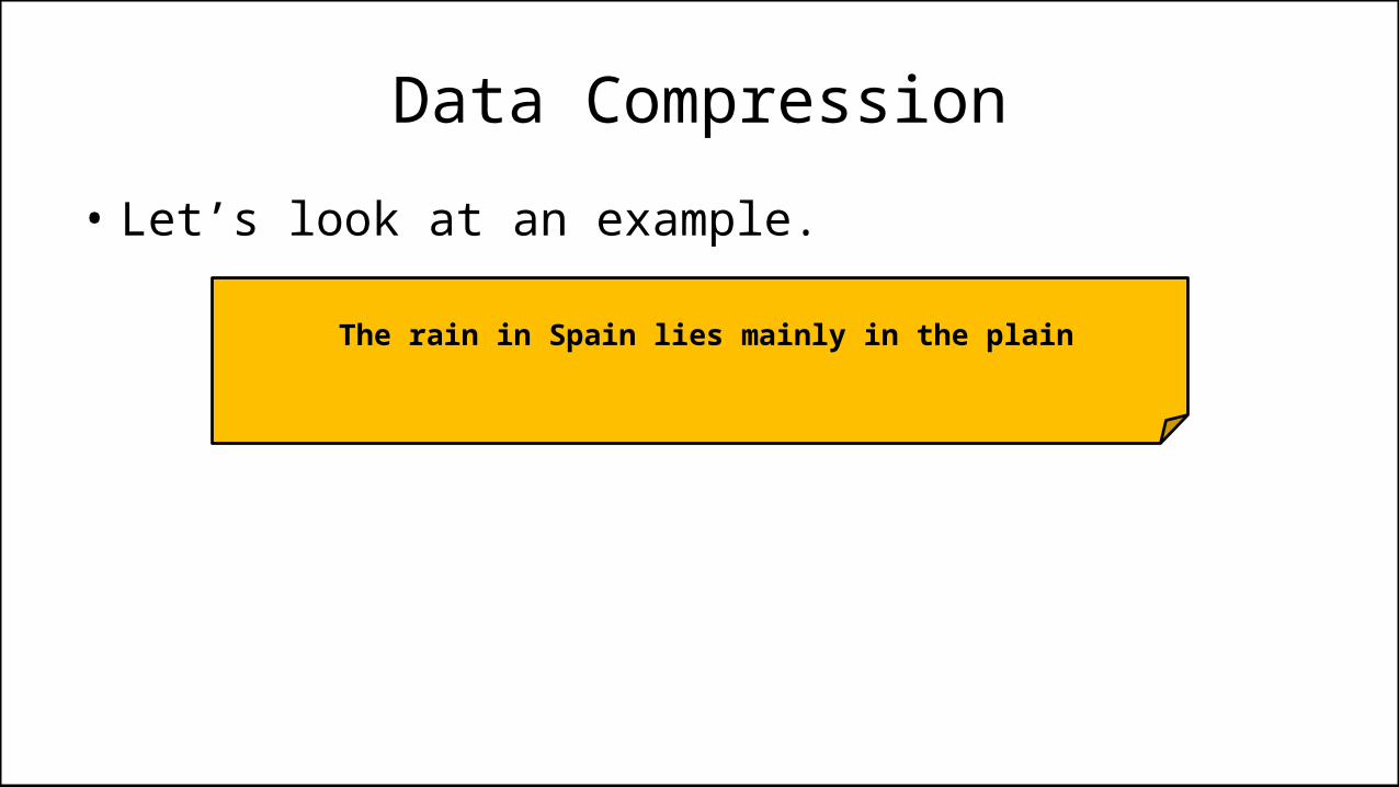
• Let’s look at an example.
The rain in Spain lies mainly in the plain
Data Compression

Data Compression
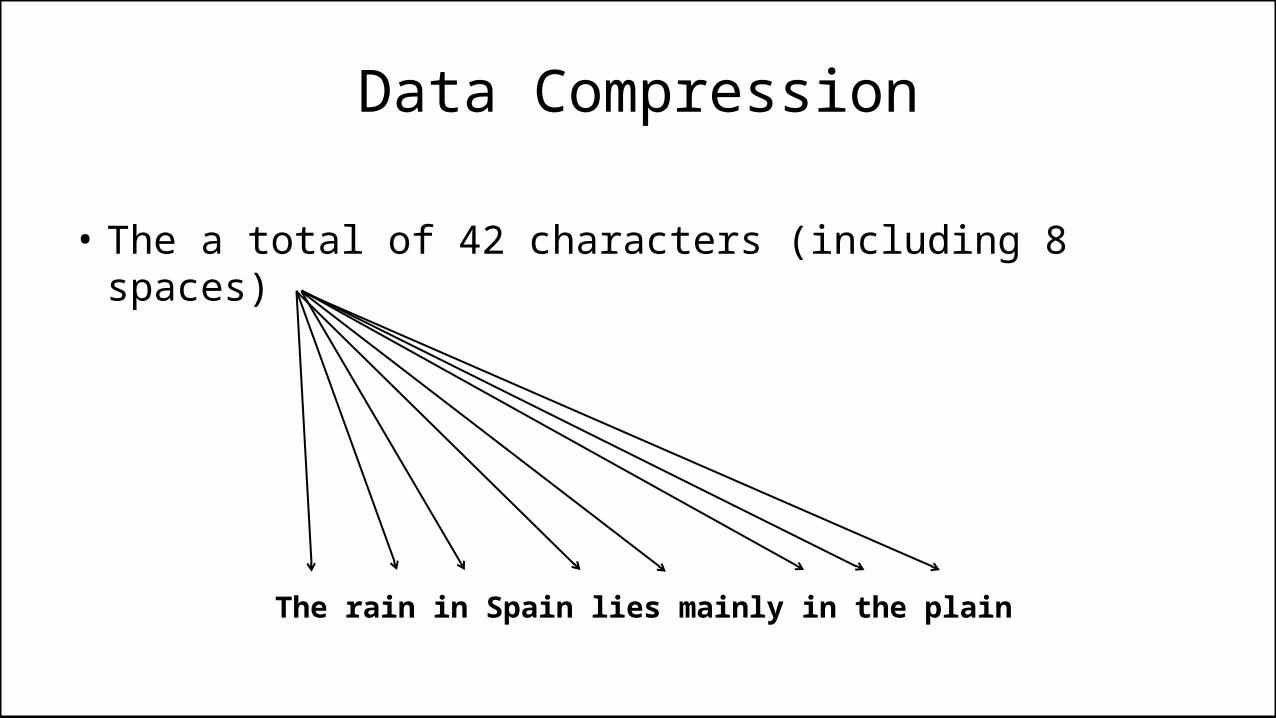
• The a total of 42 characters (including 8 spaces)
The rain in Spain lies mainly in the plain
Data Compression
• The a total of 42 characters (including 8 spaces)
The rain in Spain lies mainly in the plain

Data Compression
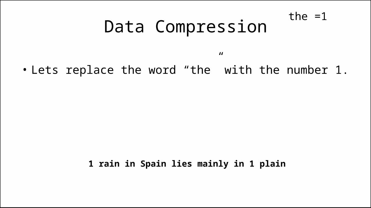
• Lets replace the word “the” with the number 1.
The rain in Spain lies mainly in the plain
Data Compression
• Lets replace the word “the” with the number 1.
1 rain in Spain lies mainly in 1 plain
the =1

Data Compression
• Lets replace the word “the” with the number 1.
• We’ve reduced the of characters to 38.
1 rain in Spain lies mainly in 1 plain
the =1

Data Compression
• Lets replace the letters “ain” with the number 2.
1 rain in Spain lies mainly in 1 plain
the =1
Data Compression
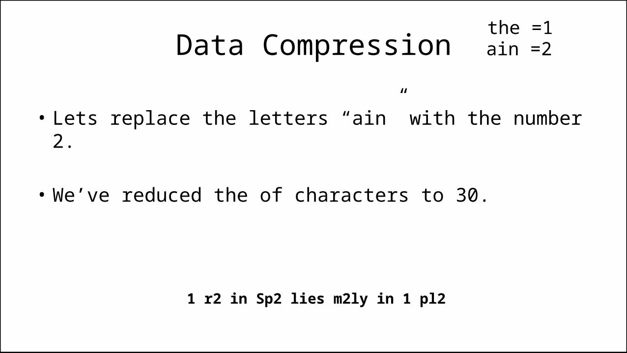
• Lets replace the letters “ain” with the number 2.
• We’ve reduced the of characters to 30.
1 r2 in Sp2 lies m2ly in 1 pl2
the =1ain =2

Data Compression
• Lets replace the letters “in” with the number 3.
1 r2 in Sp2 lies m2ly in 1 pl2
the =1ain =2

Data Compression
• Lets replace the letters “in” with the number 3.
• We’ve reduced the of characters to 28.
1 r2 3 Sp2 lies m2ly 3 1 pl2
the =1ain =2in = 3

Data Compression
• Now lets say 1 means “the ”, so it’s “the” and a space
1 r2 3 Sp2 lies m2ly 3 1 pl2
the =1ain =2in = 3

Data Compression
• Now lets say 1 means “the ”, so it’s “the” and a space
• We’ve reduced the of characters to 26.
1r2 3 Sp2 lies m2ly 3 1pl2
the =1ain =2in = 3

Data Compression
• Now lets say 3 means “in ”, so it’s “in” and a space
1r2 3 Sp2 lies m2ly 3 1pl2
the =1ain =2in = 3

Data Compression
• Now lets say 3 means “in ”, so it’s “in” and a space
• We’ve reduced the of characters to 24.
1r2 3Sp2 lies m2ly 31pl2
the =1ain =2in = 3

Data Compression
• So that’s 24 characters for a 42 character message, not bad.
The rain in Spain lies mainly in the plain
1r2 3Sp2 lies m2ly 31pl2
the =1ain =2in = 3
Data Compression
• Let’s try a different example.

Data Compression
• Let’s try a different example. Let’s say we are sending a list of jobs, with each item on the list is 10 characters long.
• Bookkeeper• Teacher---• Porter----• Nurse-----• Doctor----
Data Compression
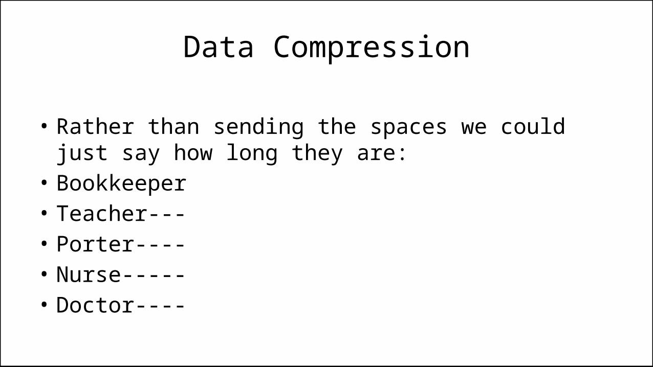
• Rather than sending the spaces we could just say how long they are:
• Bookkeeper• Teacher---• Porter----• Nurse-----• Doctor----

Data Compression
• Rather than sending the spaces we could just say how long they are:
• Bookkeeper• Teacher---• Porter----• Nurse-----• Doctor----
• Bookkeeper• Teacher3-• Porter4-• Nurse5-• Doctor4-

Data Compression
• We’ve gone from 50 to 42 characters:
• Bookkeeper• Teacher---• Porter----• Nurse-----• Doctor----
• Bookkeeper• Teacher3-• Porter4-• Nurse5-• Doctor4-

PROGRAM CompressExample:Get Current Character;WHILE (NOT End_of_Line) DO Get Next Character; IF (Current Character != Next Character) THEN Get next char, and set current to next; Write out Current Character; ELSE Keep looping while the characters match; Keep counting; Get next char, and set current to next; When finished write out Counter; Write out Current Character; Reset Counter; ENDIF; ENDWHILE;END.

PROGRAM CompressExample:char Current_Char, Next_char;Current_Char <- Get_char();WHILE (NOT End_of_Line) DO Next_Char <- Get_char(); IF (Current_Char != Next_char) THEN Current_Char <- Next_Char; Next_Char <- Get_char(); Write out Current_Char; ELSE WHILE (Current_Char = Next_char) DO Counter <- Counter + 1; Current_Char <- Next_Char; Next_Char <- Get_char(); ENDWHILE; Write out Counter, Current_Char; Counter <- 0; ENDIF; ENDWHILE;END.

Data Compression
• Or let’s imagine we are sending a list of house prices.• 350000• 600000• 550000• 2100000• 3000000

Data Compression
• Now let’s use the # to indicate number of zeros:• 350000• 600000• 550000• 2100000• 3000000
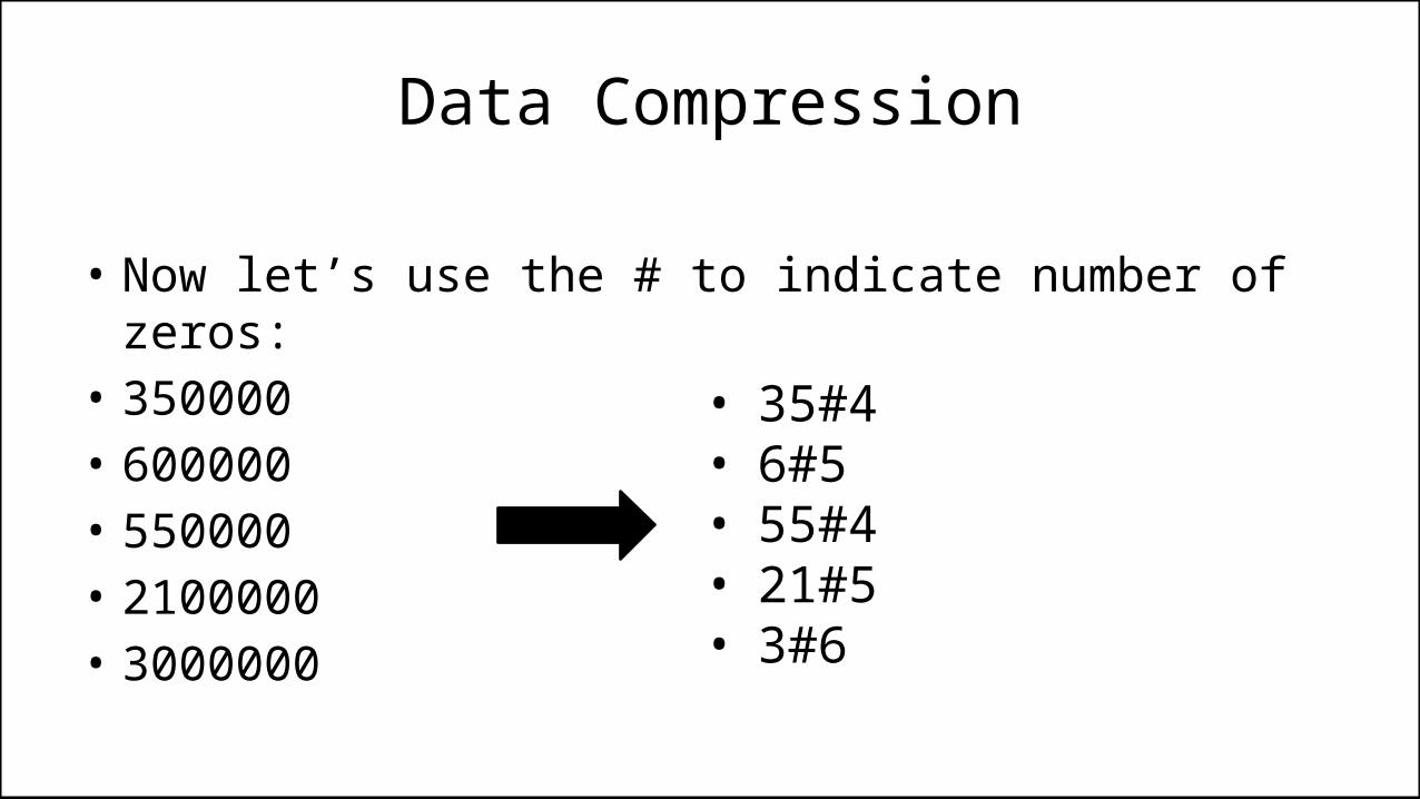
Data Compression
• Now let’s use the # to indicate number of zeros:• 350000• 600000• 550000• 2100000• 3000000
• 35#4• 6#5• 55#4• 21#5• 3#6

Data Compression
• We’ve gone from 32 characters to 18 characters:• 350000• 600000• 550000• 2100000• 3000000
• 35#4• 6#5• 55#4• 21#5• 3#6

Image Compression

Data Compression
• Let’s think about images.
• Let’s say we are trying to display the letter ‘A’

Data Compression
• Let’s think about images.
• Let’s say we are trying to display the letter ‘A’

Data Compression
• We could encode this as:
• WWWBBWWW• WWBWWBWW• WBWWWWBW• WBWWWWBW• WBBBBBBW• WBWWWWBW• WBWWWWBW• WWWWWWWW

Data Compression
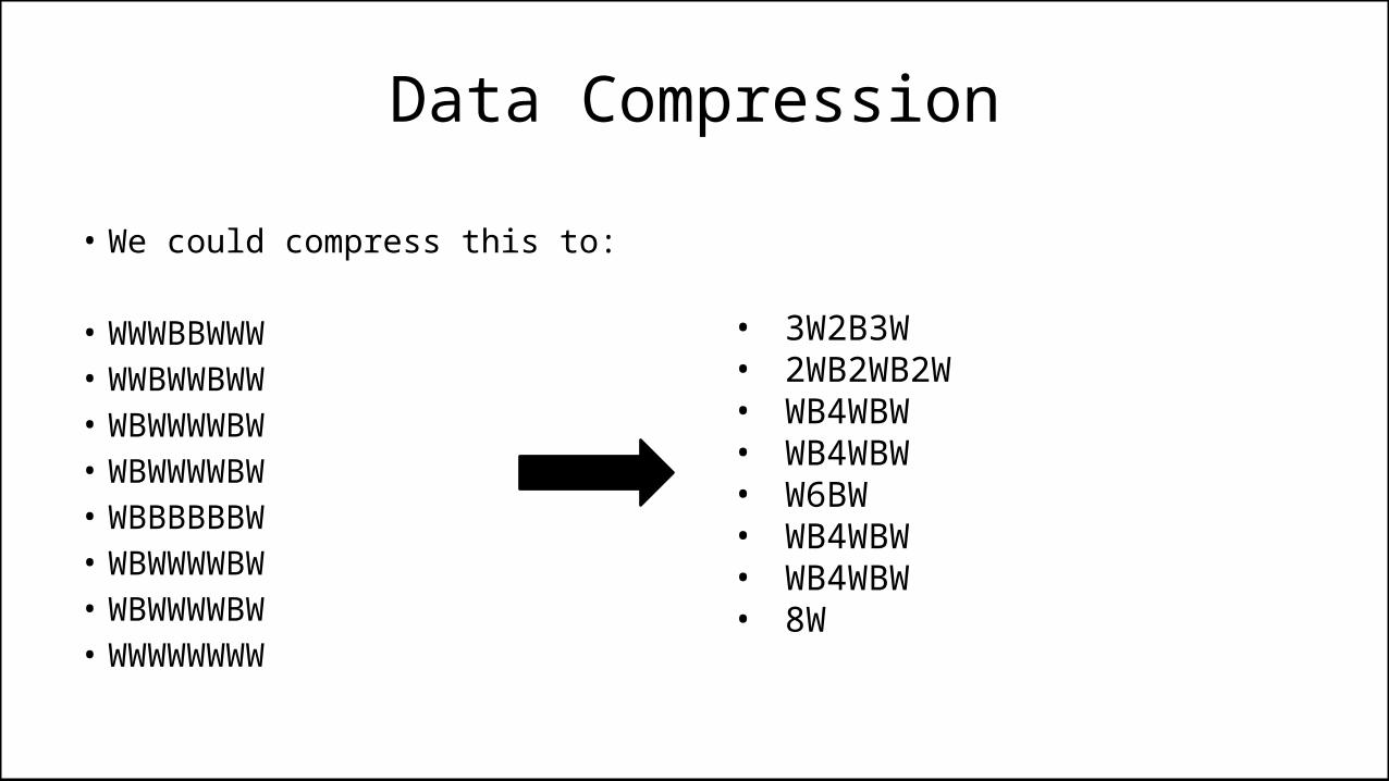
• We could compress this to:
• WWWBBWWW• WWBWWBWW• WBWWWWBW• WBWWWWBW• WBBBBBBW• WBWWWWBW• WBWWWWBW• WWWWWWWW
Data Compression
• We could compress this to:
• WWWBBWWW• WWBWWBWW• WBWWWWBW• WBWWWWBW• WBBBBBBW• WBWWWWBW• WBWWWWBW• WWWWWWWW
• 3W2B3W• 2WB2WB2W• WB4WBW• WB4WBW• W6BW• WB4WBW• WB4WBW• 8W

Data Compression
• From 64 characters to 44 characters:
• WWWBBWWW• WWBWWBWW• WBWWWWBW• WBWWWWBW• WBBBBBBW• WBWWWWBW• WBWWWWBW• WWWWWWWW
• 3W2B3W• 2WB2WB2W• WB4WBW• WB4WBW• W6BW• WB4WBW• WB4WBW• 8W
Data Compression
• We call this “run-length encoding” or RLE.

Data Compression
• Now let’s add one more rule.

Data Compression
• Now let’s add one more rule.
• Let’s imagine if we send the number ‘0’ it means repeat the previous line.

Data Compression
• So now we had:
• WWWBBWWW• WWBWWBWW• WBWWWWBW• WBWWWWBW• WBBBBBBW• WBWWWWBW• WBWWWWBW• WWWWWWWW
• 3W2B3W• 2WB2WB2W• WB4WBW• WB4WBW• W6BW• WB4WBW• WB4WBW• 8W
Data Compression
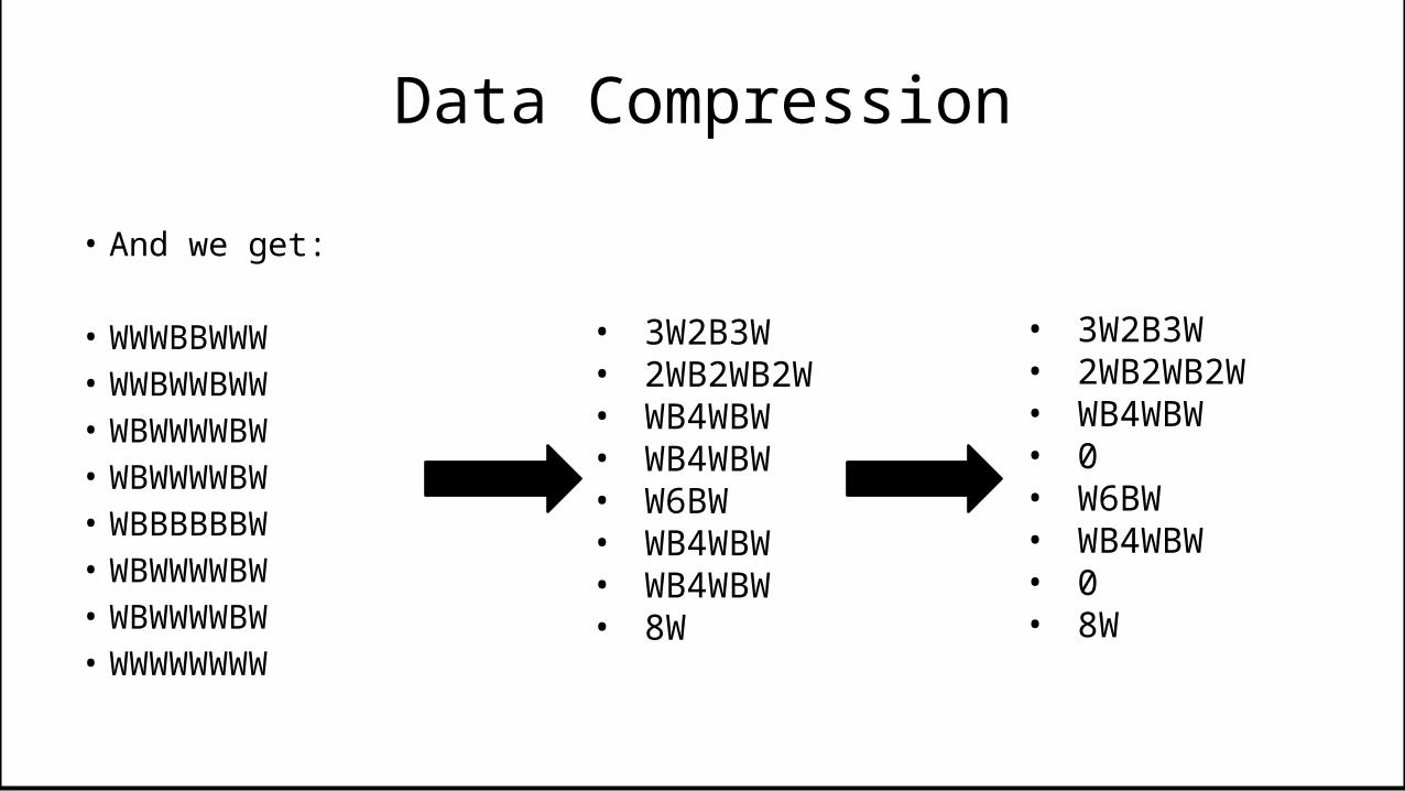
• And we get:
• WWWBBWWW• WWBWWBWW• WBWWWWBW• WBWWWWBW• WBBBBBBW• WBWWWWBW• WBWWWWBW• WWWWWWWW
• 3W2B3W• 2WB2WB2W• WB4WBW• WB4WBW• W6BW• WB4WBW• WB4WBW• 8W
• 3W2B3W• 2WB2WB2W• WB4WBW• 0• W6BW• WB4WBW• 0• 8W

Data Compression
• Going from 64 to 44 to 34 characters:
• WWWBBWWW• WWBWWBWW• WBWWWWBW• WBWWWWBW• WBBBBBBW• WBWWWWBW• WBWWWWBW• WWWWWWWW
• 3W2B3W• 2WB2WB2W• WB4WBW• WB4WBW• W6BW• WB4WBW• WB4WBW• 8W
• 3W2B3W• 2WB2WB2W• WB4WBW• 0• W6BW• WB4WBW• 0• 8W

Data Compression
• For most images, the lines are repeated frequently, so you can get massive savings from RLE.

Data Compression

ModularisationDamian Gordon

Modularisation
• Let’s imagine we had code as follows:
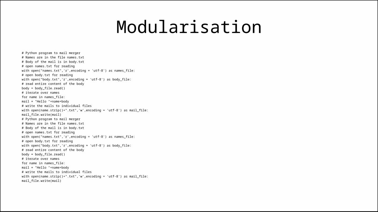
Modularisation# Python program to mail merger # Names are in the file names.txt # Body of the mail is in body.txt # open names.txt for reading with open("names.txt",'r',encoding = 'utf-8') as names_file: # open body.txt for reading with open("body.txt",'r',encoding = 'utf-8') as body_file: # read entire content of the body body = body_file.read() # iterate over names for name in names_file: mail = "Hello "+name+body # write the mails to individual files with open(name.strip()+".txt",'w',encoding = 'utf-8') as mail_file: mail_file.write(mail)# Python program to mail merger # Names are in the file names.txt # Body of the mail is in body.txt # open names.txt for reading with open("names.txt",'r',encoding = 'utf-8') as names_file: # open body.txt for reading with open("body.txt",'r',encoding = 'utf-8') as body_file: # read entire content of the body body = body_file.read() # iterate over names for name in names_file: mail = "Hello "+name+body # write the mails to individual files with open(name.strip()+".txt",'w',encoding = 'utf-8') as mail_file: mail_file.write(mail)
Modularisation
• And some bits of the code are repeated a few times

Modularisation# Python program to mail merger # Names are in the file names.txt # Body of the mail is in body.txt # open names.txt for reading with open("names.txt",'r',encoding = 'utf-8') as names_file: # open body.txt for reading with open("body.txt",'r',encoding = 'utf-8') as body_file: # read entire content of the body body = body_file.read() # iterate over names for name in names_file: mail = "Hello "+name+body # write the mails to individual files with open(name.strip()+".txt",'w',encoding = 'utf-8') as mail_file: mail_file.write(mail)# Python program to mail merger # Names are in the file names.txt # Body of the mail is in body.txt # open names.txt for reading with open("names.txt",'r',encoding = 'utf-8') as names_file: # open body.txt for reading with open("body.txt",'r',encoding = 'utf-8') as body_file: # read entire content of the body body = body_file.read() # iterate over names for name in names_file: mail = "Hello "+name+body # write the mails to individual files with open(name.strip()+".txt",'w',encoding = 'utf-8') as mail_file: mail_file.write(mail)

Modularisation# Python program to mail merger # Names are in the file names.txt # Body of the mail is in body.txt # open names.txt for reading with open("names.txt",'r',encoding = 'utf-8') as names_file: # open body.txt for reading with open("body.txt",'r',encoding = 'utf-8') as body_file: # read entire content of the body body = body_file.read() # iterate over names for name in names_file: mail = "Hello "+name+body # write the mails to individual files with open(name.strip()+".txt",'w',encoding = 'utf-8') as mail_file: mail_file.write(mail)# Python program to mail merger # Names are in the file names.txt # Body of the mail is in body.txt # open names.txt for reading with open("names.txt",'r',encoding = 'utf-8') as names_file: # open body.txt for reading with open("body.txt",'r',encoding = 'utf-8') as body_file: # read entire content of the body body = body_file.read() # iterate over names for name in names_file: mail = "Hello "+name+body # write the mails to individual files with open(name.strip()+".txt",'w',encoding = 'utf-8') as mail_file: mail_file.write(mail)

Modularisation
• It would be good if there was some way we could wrap up frequently used commands into a single package, and instead of having to rewrite the same code over and over again, we could just call the package name.
• We can call these packages methods or functions• (or subroutines or procedures)

Modularisation
• Let’s revisit our prime number algorithm again:

ModularisationPROGRAM CheckPrime: Read A; B <- A - 1; IsPrime <- TRUE; WHILE (B != 1) DO IF (A/B gives no remainder) THEN IsPrime <- FALSE; ENDIF; B <- B – 1; ENDWHILE; IF (IsPrime = FALSE) THEN Print “Not Prime”; ELSE Print “Prime”; ENDIF;END.

Modularisation
• There’s two parts to the program:

ModularisationPROGRAM CheckPrime: Read A; B <- A - 1; IsPrime <- TRUE; WHILE (B != 1) DO IF (A/B gives no remainder) THEN IsPrime <- FALSE; ENDIF; B <- B – 1; ENDWHILE; IF (IsPrime = FALSE) THEN Print “Not Prime”; ELSE Print “Prime”; ENDIF;END.

Modularisation
• The first part checks if it’s prime…• The second part just prints out the result…

Modularisation
• So we can create a module from the checking bit:

ModularisationMODULE PrimeChecker: Read A; B <- A - 1; IsPrime <- TRUE; WHILE (B != 1) DO IF (A/B gives no remainder) THEN IsPrime <- FALSE; ENDIF; B <- B – 1; ENDWHILE; RETURN IsPrime;END.

ModularisationMODULE PrimeChecker: Read A; B <- A - 1; IsPrime <- TRUE; WHILE (B != 1) DO IF (A/B gives no remainder) THEN IsPrime <- FALSE; ENDIF; B <- B – 1; ENDWHILE; RETURN IsPrime;END.

Modularisation
• Let’s remind ourselves of what the algorithm was initially.

ModularisationPROGRAM CheckPrime: Read A; B <- A - 1; IsPrime <- TRUE; WHILE (B != 1) DO IF (A/B gives no remainder) THEN IsPrime <- FALSE; ENDIF; B <- B – 1; ENDWHILE; IF (IsPrime = FALSE) THEN Print “Not Prime”; ELSE Print “Prime”; ENDIF;END.

Modularisation
• Now that we have a module to do the check we can rewrite as follows:

Modularisation
PROGRAM CheckPrime: IF (PrimeChecker = FALSE) THEN Print “Not Prime”; ELSE Print “Prime”; ENDIF;END.

ModularisationMODULE PrimeChecker: Read A; B <- A - 1; IsPrime <- TRUE; WHILE (B != 1) DO IF (A/B gives no remainder) THEN IsPrime <- FALSE; ENDIF; B <- B – 1; ENDWHILE; RETURN IsPrime;END.

Modularisation
• Modularisation make life easier for a lot of reasons:– It easier for someone else to understand how the code works– It makes team programming a lot easier, different programmers
can work on different methods– Can improve the quality of the code– Can reuse the same code over and over again (“don’t reinvent
the wheel”).

Modularisation
• If we were writing programs about primes, it would be useful to have a pre-packaged prime test, e.g.
• If we were writing a program to explore Goldbach's conjecture, that all even integers are sums of two primes, if would be useful.
• Also if we were exploring twin primes, which are prime numbers that has a gap of two, (3, 5), (5, 7), (11, 13), (17, 19), (29, 31), (41, 43), (59, 61), (71, 73), (101, 103), (107, 109), (137, 139), it would be useful.

Software TestingDamian Gordon

• Why do pilots bother doing pre-flight checks when the chances are that the plane is working fine?
Question

• Software testing is an investigate process to measure the quality of software.
• Test techniques include, but are not limited to, the process of executing a program or application with the intent of finding software bugs.
Software Testing
Software Testing
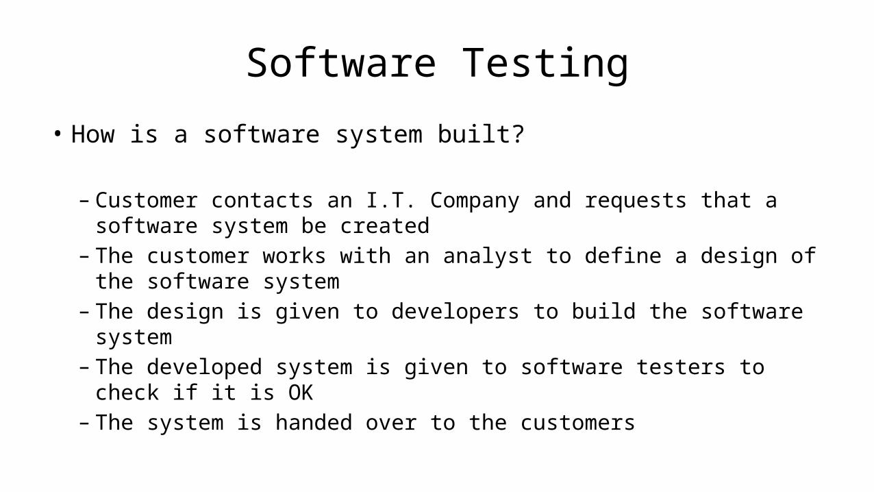
• How is a software system built?
– Customer contacts an I.T. Company and requests that a software system be created
– The customer works with an analyst to define a design of the software system
– The design is given to developers to build the software system– The developed system is given to software testers to check if it is OK– The system is handed over to the customers

• The IBM Automatic Sequence Controlled Calculator (ASCC), called the Mark I by Harvard University was an electro-mechanical computer.
• It was devised by Howard H. Aiken, built at IBM and shipped to Harvard in February 1944.
• It began computations for the U.S. Navy Bureau of Ships in May and was officially presented to the university on August 7, 1944.
• It was very reliable, much more so than early electronic computers.
Harvard Mark I1944AD

• Howard Hathaway Aiken • Born March 8, 1900• Died March 14, 1973• Born in Hoboken, New Jersey• He envisioned an electro-mechanical
computing device that could do much of the tedious work for him.
• With help from Grace Hopper and funding from IBM, the machine was completed in 1944.
Howard H. Aiken

• Rear Admiral Grace Murray Hopper
• Born December 9, 1906• Died January 1, 1992• Born in New York City, New York• Computer pioneer who
developed the first compiler for a computer programming language
Grace Hopper

• Grace Hopper served at the Bureau of Ships Computation Project at Harvard University working on the computer programming staff.
• A moth was found trapped between points at Relay #70, Panel F, of the IBM Harvard Mark II Aiken Relay Calculator while it was being tested at Harvard University, 9 September 1945.
The First Bug1945AD

• The operators affixed the moth to the computer log, with the entry: "First actual case of bug being found".
• Grace Hopper said that they "debugged" the machine, thus introducing the term "debugging a computer program".
The First Bug1945AD


Bugs a.k.a. …
• Defect• Fault• Problem• Error• Incident• Anomaly• Variance
• Failure• Inconsistency• Product Anomaly• Product Incidence

Eras of TestingYears Era Description
1945-1956 Debugging orientated In this era, there was no clear difference between testing and debugging.
1957-1978 Demonstration orientated In this era, debugging and testing are distinguished now - in this period it was shown, that software satisfies the requirements.
1979-1982 Destruction orientated In this era, the goal was to find errors.
1983-1987 Evaluation orientated In this era, the intention here is that during the software lifecycle a product evaluation is provided and measuring quality.
1988- Prevention orientated In the current era, tests are used to demonstrate that software satisfies its specification, to detect faults and to prevent faults.

Software Testing Methods

Box Approach

Box Approach
BlackBox
WhiteBox
GreyBox

• Black box testing treats the software as a "black box"—without any knowledge of internal implementation.
• Black box testing methods include: – equivalence partitioning, – boundary value analysis, – all-pairs testing, – fuzz testing, – model-based testing, – exploratory testing and – specification-based testing.
Black Box Testing
BlackBox

• White box testing is when the tester has access to the internal data structures and algorithms including the code that implement these.
• White box testing methods include: – API testing (application programming interface) - testing of the application
using public and private APIs– Code coverage - creating tests to satisfy some criteria of code coverage (e.g.,
the test designer can create tests to cause all statements in the program to be executed at least once)
– Fault injection methods - improving the coverage of a test by introducing faults to test code paths
– Mutation testing methods– Static testing - White box testing includes all static testing
White Box Testing
WhiteBox
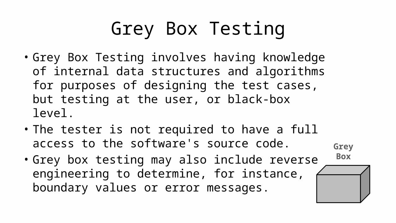
• Grey Box Testing involves having knowledge of internal data structures and algorithms for purposes of designing the test cases, but testing at the user, or black-box level.
• The tester is not required to have a full access to the software's source code.
• Grey box testing may also include reverse engineering to determine, for instance, boundary values or error messages.
Grey Box Testing
GreyBox

Types of Testing

• Lowest level functions and procedures in isolation• Each logic path in the component specifications
Unit Testing

• Tests the interaction of all the related components of a module• Tests the module as a stand-alone entity
Module Testing
• Tests the interfaces between the modules• Scenarios are employed to test module interaction
Subsystem Testing

• Tests interactions between sub-systems and components• System performance• Stress• Volume
Integration Testing

• Tests the whole system with live data• Establishes the ‘validity’ of the system
Acceptance Testing

Testing Tools

• Program testing and fault detection can be aided significantly by testing tools and debuggers. Testing/debug tools include features such as:– Program monitors, permitting full or partial monitoring of program code (more
on the next slide).– Formatted dump or symbolic debugging, tools allowing inspection of program
variables on error or at chosen points.– Automated functional GUI testing tools are used to repeat system-level tests
through the GUI.– Benchmarks, allowing run-time performance comparisons to be made.– Performance analysis (or profiling tools) that can help to highlight hot spots and
resource usage.
Testing Tools

• Program monitors, permitting full or partial monitoring of program code including:– Instruction set simulator, permitting complete instruction level
monitoring and trace facilities– Program animation, permitting step-by-step execution and
conditional breakpoint at source level or in machine code– Code coverage reports
Testing Tools
Data Structures:Arrays
Damian Gordon

Arrays
• Imagine we had to record the age of everyone in the class, we could do it declaring a variable for each person.

Arrays
• Imagine we had to record the age of everyone in the class, we could do it declaring a variable for each person.
• E.g.– Integer Age1;– Integer Age2;– Integer Age3;– Integer Age4;– Integer Age5;– etc.
Arrays
• But if there was a way to collect them all together, and declare a single special variable for all of them, that would be quicker.
• We can, and the special variable is called an array.

Arrays
• We declare an array as follows:
• Integer Age[40];

Arrays
• We declare an array as follows:
• Integer Age[40];
• Which means we declare 40 integer variables, all can be accessed using the Age name.
……..…Age

Arrays
• We declare an array as follows:
• Integer Age[40];
• Which means we declare 40 integer variables, all can be accessed using the Age name.
0 1 2 3 4 5 6 397 ……..… 38Age

Arrays
44 23 42 33 16 - - 34 8218 ……..… 340 1 2 3 4 5 6 7 38 39Age

Arrays
44 23 42 33 16 - - 34 8218 ……..… 340 1 2 3 4 5 6 7 38 39
• So if I do:• PRINT Age[0];
• We will get:• 44
Age

Arrays
44 23 42 33 16 - - 34 8218 ……..… 340 1 2 3 4 5 6 7 38 39
• So if I do:• PRINT Age[2];
• We will get:• 42
Age

Arrays
44 23 42 33 16 - - 34 8218 ……..… 340 1 2 3 4 5 6 7 38 39
• So if I do:• PRINT Age[39];
• We will get:• 82
Age

Arrays
44 23 42 33 16 - - 34 8218 ……..… 340 1 2 3 4 5 6 7 38 39
• So if I do:• PRINT Age[40];
• We will get:• Array Out of Bounds Exception
Age

Arrays
44 23 42 33 16 - - 34 8218 ……..… 340 1 2 3 4 5 6 7 38 39
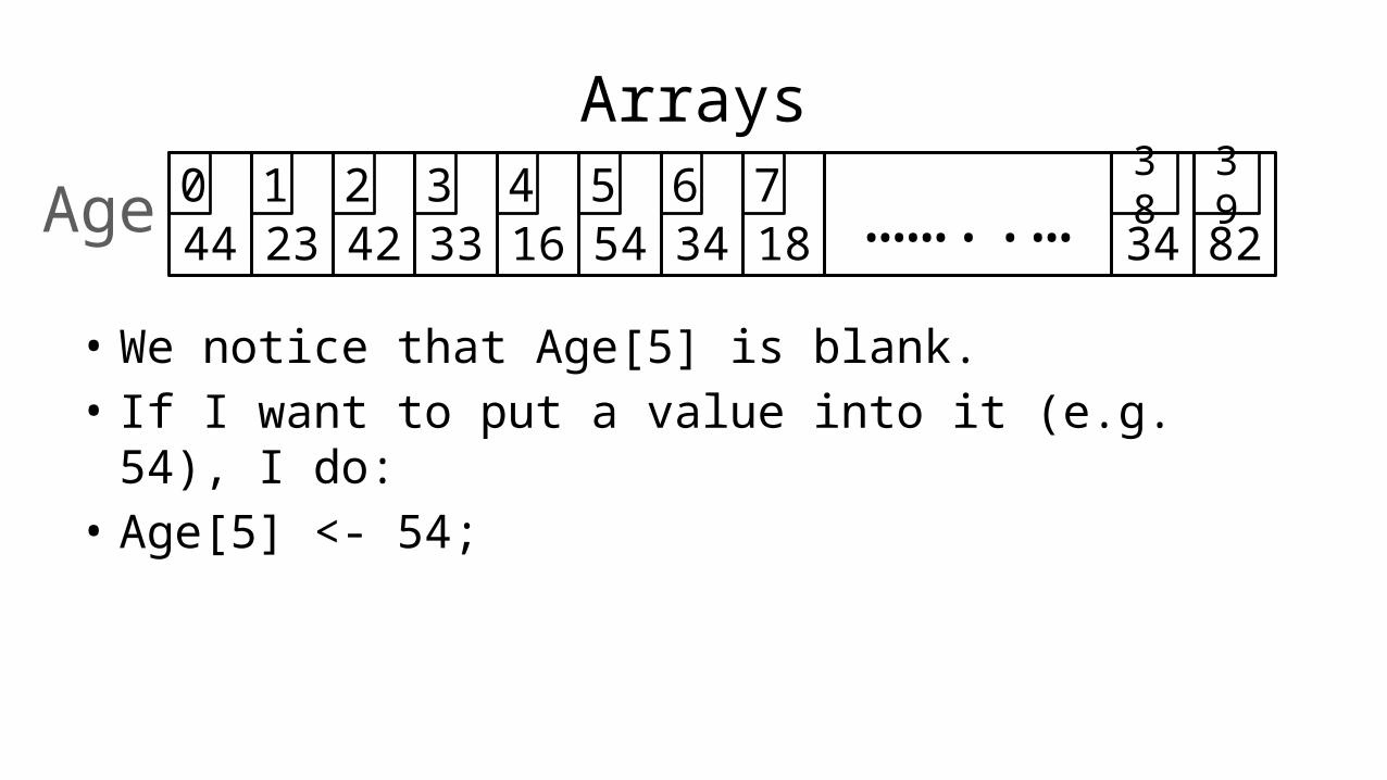
• We notice that Age[5] is blank. • If I want to put a value into it (e.g. 54), I do:• Age[5] <- 54;
Age
Arrays
44 23 42 33 16 54 34 8218 ……..… 340 1 2 3 4 5 6 7 38 39
• We notice that Age[5] is blank. • If I want to put a value into it (e.g. 54), I do:• Age[5] <- 54;
Age

Arrays
• We can think of an array as a series of pigeon-holes:

Array
9 10 11
12 13 14
1516
1819
1 2
3 4 5
6 7 8
0
17
20

Arrays
• If we look at our array again:
44 23 42 33 16 54 34 8218 ……..… 340 1 2 3 4 5 6 7 38 39Age

Arrays
• If we wanted to add 1 to everyone’s age:
44 23 42 33 16 54 34 8218 ……..… 340 1 2 3 4 5 6 7 38 39Age+1 +1 +1 +1 +1 +1 +1 +1 +1 +1

Arrays
• If we wanted to add 1 to everyone’s age:
45 24 43 34 17 55 35 8319 ……..… 350 1 2 3 4 5 6 7 38 39Age

Arrays
• We could do it like this:PROGRAM Add1ToAge: Age[0] <- Age[0] + 1; Age[1] <- Age[1] + 1; Age[2] <- Age[2] + 1; Age[3] <- Age[3] + 1; Age[4] <- Age[4] + 1; Age[5] <- Age[5] + 1; ……………………………………………………… Age[38] <- Age[38] + 1; Age[39] <- Age[39] + 1;END.

Arrays
• An easier way of doing it is:
PROGRAM Add1ToAge: N <- 0; WHILE (N != 40) DO Age[N] <- Age[N] + 1; N <- N + 1; ENDWHILE;END.

Arrays
• Or:
PROGRAM Add1ToAge: FOR N IN 0 TO 39 DO Age[N] <- Age[N] + 1; ENDFOR;END.

Arrays
• If we want to add up all the values in the array:

Arrays
• If we want to add up all the values in the array:
PROGRAM TotalOfArray: integer Total <- 0; FOR N IN 0 TO 39 DO Total <- Total + Age[N]; ENDFOR;END.

Arrays
• So the average age is:

Arrays
• So the average age is:
PROGRAM AverageOfArray: integer Total <- 0; FOR N IN 0 TO 39 DO Total <- Total + Age[N]; ENDFOR; PRINT Total/40;END.

Arrays
• We can add another variable:
PROGRAM AverageOfArray: integer Total <- 0; integer ArraySize <- 40; FOR N IN 0 TO 39 DO Total <- Total + Age[N]; ENDFOR; PRINT Total/40;END.

Arrays
• We can add another variable:
PROGRAM AverageOfArray: integer Total <- 0; integer ArraySize <- 40; FOR N IN 0 TO 39 DO Total <- Total + Age[N]; ENDFOR; PRINT Total/ArraySize;END.

Arrays
• We can add another variable:
PROGRAM AverageOfArray: integer Total <- 0; integer ArraySize <- 40; FOR N IN 0 TO ArraySize-1 DO Total <- Total + Age[N]; ENDFOR; PRINT Total/ArraySize;END.

• So now if the Array size changes, we just need to change the value of one variable (ArraySize).
PROGRAM AverageOfArray: integer Total <- 0; integer ArraySize <- 40; FOR N IN 0 TO ArraySize-1 DO Total <- Total + Age[N]; ENDFOR; PRINT Total/ArraySize;END.
Arrays

Arrays
• We can also have an array of real numbers:

Arrays
• We can also have an array of real numbers:
22.000Bank
Balance 65.501
-2.202
78.80 54.00 -3.33 0.00 47.653 4 5 6 7

• What if we wanted to check who has a balance less than zero :PROGRAM LessThanZeroBalance: integer ArraySize <- 8; FOR N IN 0 TO ArraySize-1 DO IF BankBalance[N] < 0 THEN PRINT “User” N “is in debt”; ENDIF; ENDFOR;END.
Arrays

Arrays
• We can also have an array of characters:

Arrays
• We can also have an array of characters:
G A T T C C A AG ……..… A0 1 2 3 4 5 6 7 38 39Gene

• What if we wanted to count all the ‘G’ in the Gene Array:
Arrays
G A T T C C A AG ……..… A0 1 2 3 4 5 6 7 38 39Gene

• What if we wanted to count all the ‘G’ in the Gene Array:PROGRAM AverageOfArray: integer ArraySize <- 40; integer G-Count <- 0; FOR N IN 0 TO ArraySize-1 DO IF Gene[N] = ‘G’ THEN G-Count <- G-Count + 1; ENDIF; ENDFOR; PRINT “The total G count is:” G-Count;END.
Arrays

• What if we wanted to count all the ‘A’ in the Gene Array:PROGRAM AverageOfArray: integer ArraySize <- 40; integer A-Count <- 0; FOR N IN 0 TO ArraySize-1 DO IF Gene[N] = ‘A’ THEN A-Count <- A-Count + 1; ENDIF; ENDFOR; PRINT “The total A count is:” A-Count;END.
Arrays

Arrays
• We can also have an array of strings:

Arrays
• We can also have an array of strings:
Dog0
Pets Cat1
Dog2
Bird Fish Fish Cat Cat3 4 5 6 7

Arrays
• We can also have an array of booleans:

Arrays
• We can also have an array of booleans:
TRUE0In
School TRUE1
FALSE2
TRUE FALSE TRUE FALSE FALSE3 4 5 6 7

SearchingDamian Gordon

Google PageRankDamian Gordon


Google Search Algorithm
• First Draft:PROGRAM GoogleCollect: NextLink <- random website; WHILE (NextLink != NULL) DO IF (No copy of this page in google collection) THEN copy this page into google collection; ENDIF; NextLink <- Next link on this page; ENDWHILE;END.

Google Search Algorithm
• First Draft:PROGRAM GoogleSearch: READ SearchString; Get First Webpage from collection; WHILE (Webpages Left to Search) DO IF (SearchString IN Current-Web-Page) THEN Put this page on the list; ENDIF; Get Next Webpage; ENDWHILE; Order the list according to PageRank;END.


Database SearchingDamian Gordon

Searching
• Oracle• DB2• MySQL• SQL Server• PostgreSQL

Searching

Array SearchingDamian Gordon

Searching
• Let’s remember our integer array from before:

Searching
44 23 42 33 16 54 34 8218 ……..… 340 1 2 3 4 5 6 7 38 39Age

Searching
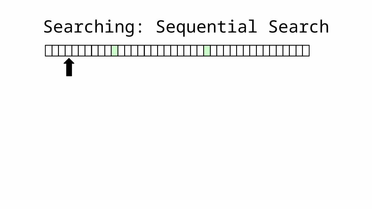
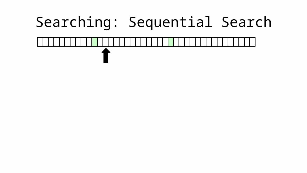
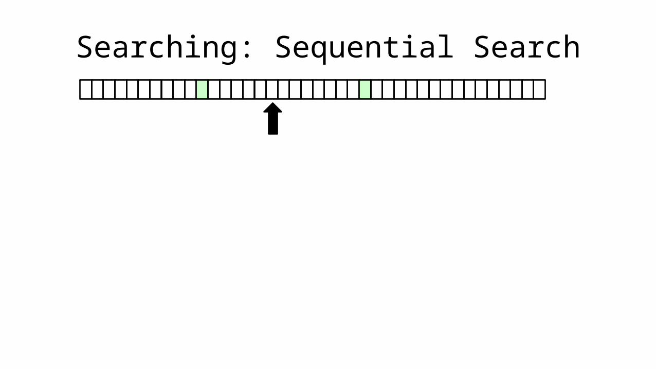
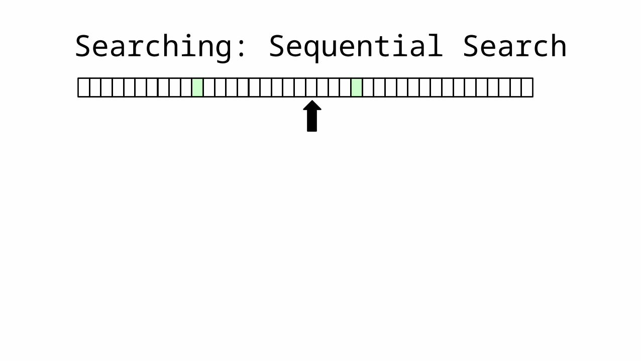
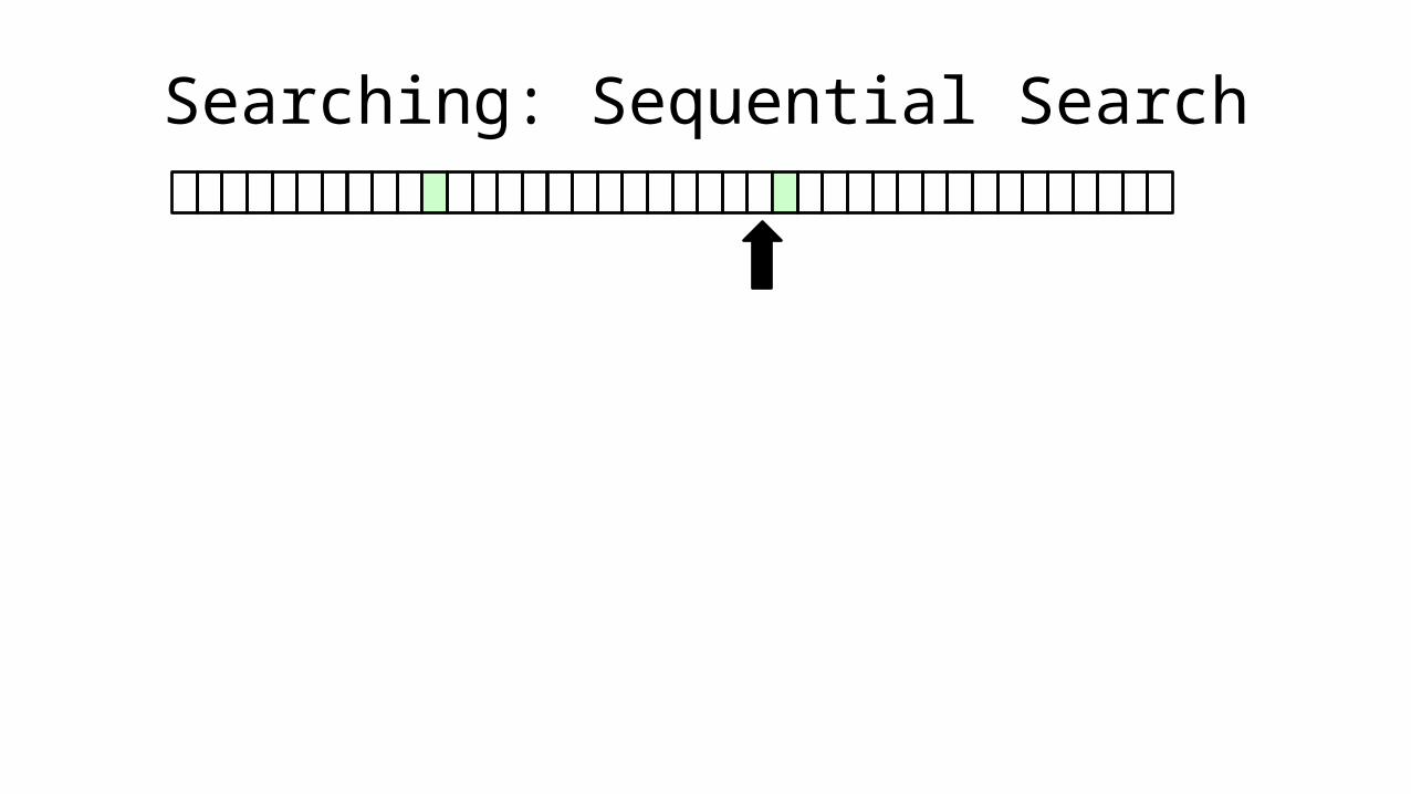
• Let’s say we want to find everyone who is aged 18:
Searching: Sequential Search

Searching: Sequential Search

Searching: Sequential Search

Searching: Sequential Search
Searching: Sequential Search

Searching: Sequential Search

Searching: Sequential Search

Searching: Sequential Search

Searching: Sequential Search

Searching: Sequential Search

Searching: Sequential Search

Searching: Sequential Search

Searching: Sequential Search
Searching: Sequential Search

Searching: Sequential Search

Searching: Sequential Search

Searching: Sequential Search
Searching: Sequential Search

Searching: Sequential Search

Searching: Sequential Search

Searching: Sequential Search
Searching: Sequential Search

Searching: Sequential Search

Searching: Sequential Search
Searching: Sequential Search

Searching: Sequential Search

Searching: Sequential Search

Searching: Sequential Search

Searching: Sequential Search

Searching: Sequential Search

Searching: Sequential Search

Searching: Sequential Search

Searching: Sequential Search

Searching: Sequential Search

Searching: Sequential Search

Searching: Sequential Search

Searching: Sequential Search

Searching: Sequential Search

Searching: Sequential Search

Searching: Sequential Search

Searching: Sequential Search

Searching: Sequential Search
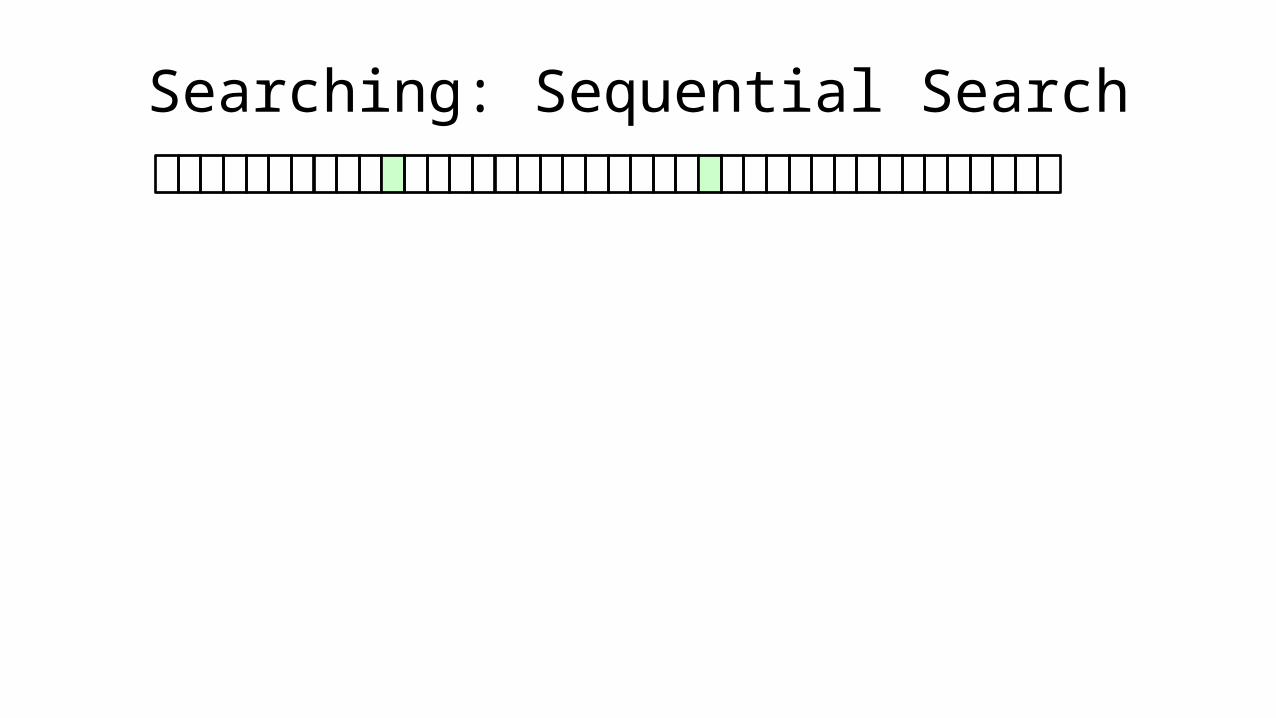
• This is a SEQUENTIAL SEARCH.
• If the array is 40 characters long, it will take 40 checks to complete. If the array is 1000 characters long, it will take 1000 checks to complete.
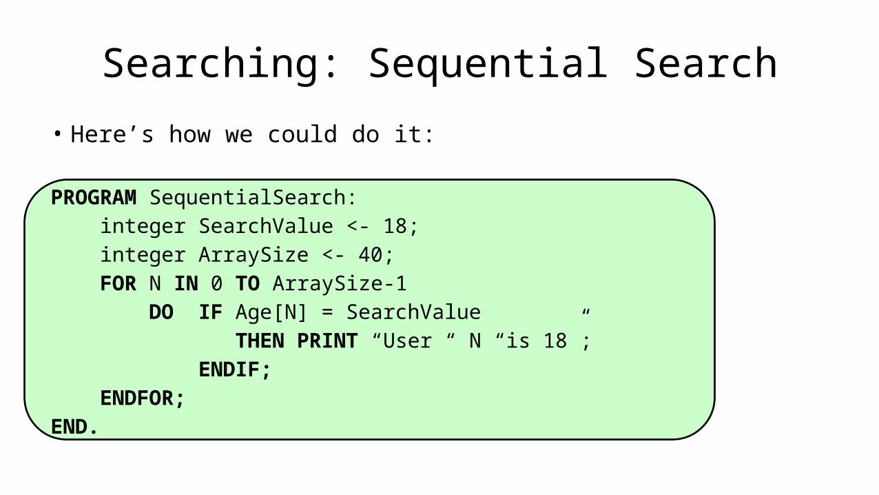
• Here’s how we could do it:
PROGRAM SequentialSearch: integer SearchValue <- 18; integer ArraySize <- 40; FOR N IN 0 TO ArraySize-1 DO IF Age[N] = SearchValue THEN PRINT “User “ N “is 18”; ENDIF; ENDFOR;END.
Searching: Sequential Search

Searching: Binary Search
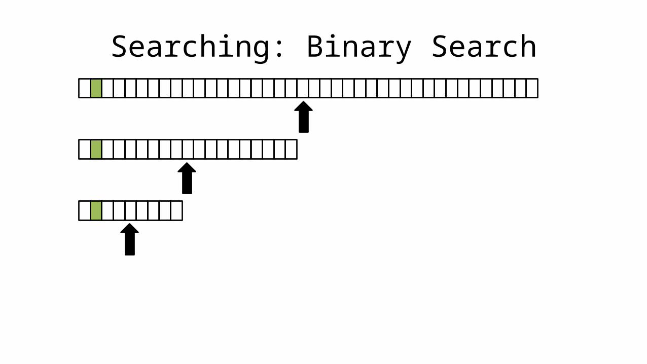
• If the data is sorted, we can do a BINARY SEARCH

Searching: Binary Search
• If the data is sorted, we can do a BINARY SEARCH
16 18 23 23 33 33 34 8243 ……..… 780 1 2 3 4 5 6 7 38 39Age

Searching: Binary Search
• If the data is sorted, we can do a BINARY SEARCH

Searching: Binary Search
• If the data is sorted, we can do a BINARY SEARCH
• This means we jump to the middle of the array, if the value being searched for is less than the middle value, all we have to do is search the first half of that array.

Searching: Binary Search
• If the data is sorted, we can do a BINARY SEARCH
• This means we jump to the middle of the array, if the value being searched for is less than the middle value, all we have to do is search the first half of that array.
• We search the first half of the array in the same way, jumping to the middle of it, and repeat this.

Searching: Binary Search

Searching: Binary Search

Searching: Binary Search

Searching: Binary Search

Searching: Binary Search
Searching: Binary Search

Searching: Binary Search

Searching: Binary Search

Searching: Binary Search

Searching: Binary Search

Searching: Binary Search
• The BINARY SEARCH just takes five checks to find the right value in an array of 40 elements. For an array of 1000 elements it will take 11 checks.
• This is much faster than if we searched through all the values.

• If the data is sorted, we can do a BINARY SEARCH
PROGRAM BinarySearch: integer First <- 0; integer Last <- 40; boolean IsFound <- FALSE; WHILE First <= Last AND IsFound = FALSE DO Index = (First + Last)/2; IF Age[Index] = SearchValue THEN IsFound <- TRUE; ELSE IF Age[Index] > SearchValue THEN Last <- Index-1; ELSE First <- Index+1; ENDIF; ENDIF; ENDWHILE;END.
Searching: Binary Search

SortingDamian Gordon

Sorting
• Let’s remember our integer array from before:

Sorting
44 23 42 33 16 54 34 180 1 2 3 4 5 6 7Age
Sorting
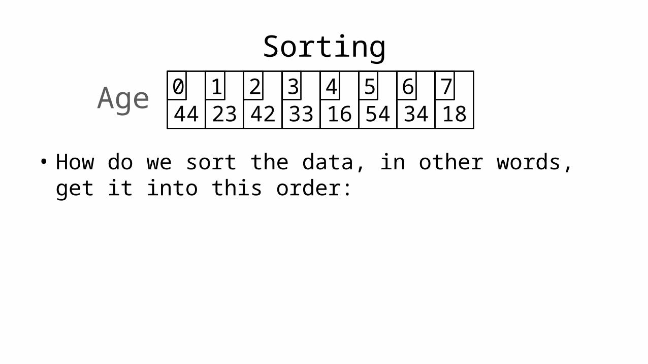
44 23 42 33 16 54 34 180 1 2 3 4 5 6 7Age
• How do we sort the data, in other words, get it into this order:

Sorting
44 23 42 33 16 54 34 180 1 2 3 4 5 6 7Age
• How do we sort the data, in other words, get it into this order:
16 18 23 33 34 42 44 540 1 2 3 4 5 6 7Age

Sorting
• As humans, we can sort the array just by inspection (just be looking at it), but if the array was 100,000 elements long it would be more of a challenge for us.

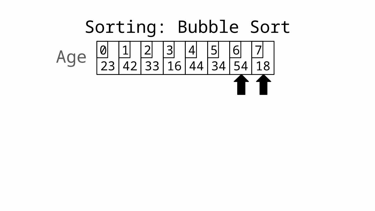
Sorting: Bubble Sort
• The simplest algorithm for sort an array is called BUBBLE SORT.

Sorting: Bubble Sort
• The simplest algorithm for sort an array is called BUBBLE SORT.
• It works as follows:

Sorting: Bubble Sort
• The simplest algorithm for sort an array is called BUBBLE SORT.
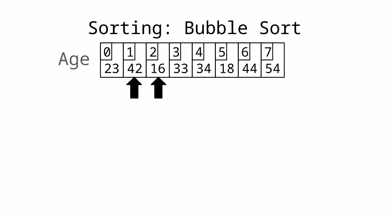
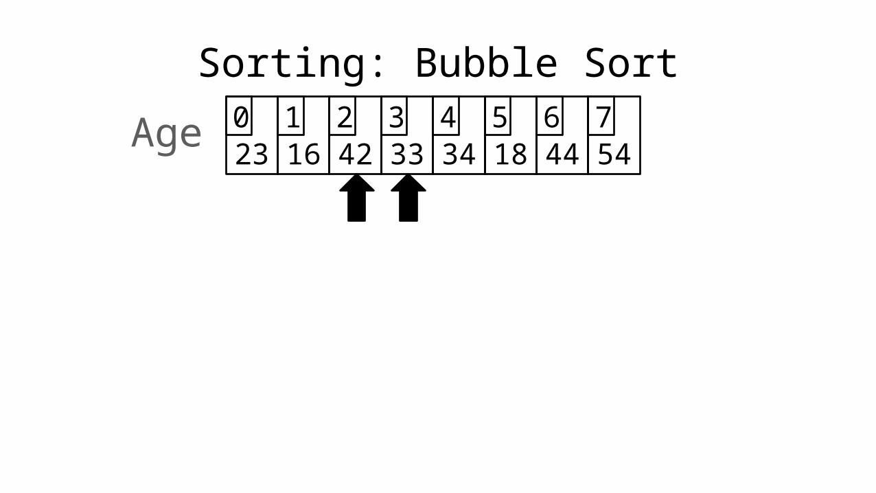
• It works as follows for an array of size N:– Look at the first and second element
• Are they in order?• If so, do nothing• If not, swap them around
– Look at the second and third element • Do the same
– Keep doing this until you get to the end of the array– Go back to the start again keep doing this whole process for N times.

• Lets look at the swapping bit– if I wanted to swap two values, the following won’t work:
Age[0] <- Age[1];Age[1] <- Age[0];
– Why not?
Sorting: Bubble Sort

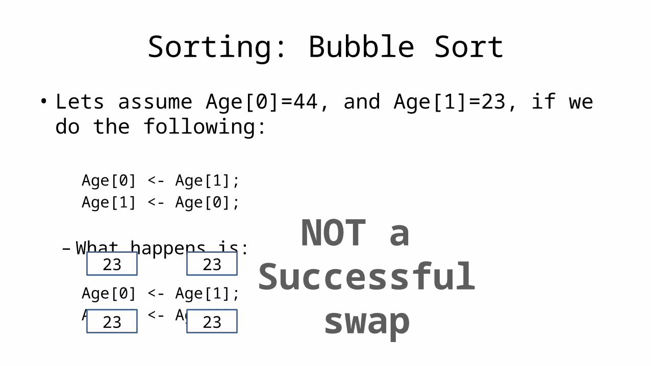
• Lets assume Age[0]=44, and Age[1]=23, if we do the following:
Age[0] <- Age[1];Age[1] <- Age[0];
– What happens is:
Age[0] <- Age[1];Age[1] <- Age[0];
Sorting: Bubble Sort

• Lets assume Age[0]=44, and Age[1]=23, if we do the following:
Age[0] <- Age[1];Age[1] <- Age[0];
– What happens is:
Age[0] <- Age[1];Age[1] <- Age[0];
Sorting: Bubble Sort
23

• Lets assume Age[0]=44, and Age[1]=23, if we do the following:
Age[0] <- Age[1];Age[1] <- Age[0];
– What happens is:
Age[0] <- Age[1];Age[1] <- Age[0];
Sorting: Bubble Sort
2323

• Lets assume Age[0]=44, and Age[1]=23, if we do the following:
Age[0] <- Age[1];Age[1] <- Age[0];
– What happens is:
Age[0] <- Age[1];Age[1] <- Age[0];
Sorting: Bubble Sort
2323
23

• Lets assume Age[0]=44, and Age[1]=23, if we do the following:
Age[0] <- Age[1];Age[1] <- Age[0];
– What happens is:
Age[0] <- Age[1];Age[1] <- Age[0];
Sorting: Bubble Sort
2323
2323
• Lets assume Age[0]=44, and Age[1]=23, if we do the following:
Age[0] <- Age[1];Age[1] <- Age[0];
– What happens is:
Age[0] <- Age[1];Age[1] <- Age[0];
Sorting: Bubble Sort
2323
2323
NOT a Successful
swap

• Lets assume Age[0]=44, and Age[1]=23, if we do the following:
Age[0] <- Age[1];Age[1] <- Age[0];
– What happens is:
Age[0] <- Age[1];Age[1] <- Age[0];
Sorting: Bubble Sort
2323
2323
NOT a Successful
swap
Age[0]=23Age[1]=23

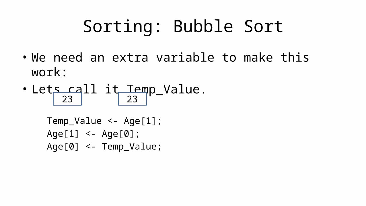
• We need an extra variable to make this work:
Sorting: Bubble Sort

• We need an extra variable to make this work:• Lets call it Temp_Value.
Sorting: Bubble Sort

• We need an extra variable to make this work:• Lets call it Temp_Value.
Temp_Value <- Age[1];
Sorting: Bubble Sort

• We need an extra variable to make this work:• Lets call it Temp_Value.
Temp_Value <- Age[1];Age[1] <- Age[0];
Sorting: Bubble Sort

• We need an extra variable to make this work:• Lets call it Temp_Value.
Temp_Value <- Age[1];Age[1] <- Age[0];Age[0] <- Temp_Value;
Sorting: Bubble Sort

• We need an extra variable to make this work:• Lets call it Temp_Value.
Temp_Value <- Age[1];Age[1] <- Age[0];Age[0] <- Temp_Value;
Sorting: Bubble Sort
23
• We need an extra variable to make this work:• Lets call it Temp_Value.
Temp_Value <- Age[1];Age[1] <- Age[0];Age[0] <- Temp_Value;
Sorting: Bubble Sort
2323

• We need an extra variable to make this work:• Lets call it Temp_Value.
Temp_Value <- Age[1];Age[1] <- Age[0];Age[0] <- Temp_Value;
Sorting: Bubble Sort
2323
44

• We need an extra variable to make this work:• Lets call it Temp_Value.
Temp_Value <- Age[1];Age[1] <- Age[0];Age[0] <- Temp_Value;
Sorting: Bubble Sort
2323
4444

• We need an extra variable to make this work:• Lets call it Temp_Value.
Temp_Value <- Age[1];Age[1] <- Age[0];Age[0] <- Temp_Value;
Sorting: Bubble Sort
2323
4444
23

• We need an extra variable to make this work:• Lets call it Temp_Value.
Temp_Value <- Age[1];Age[1] <- Age[0];Age[0] <- Temp_Value;
Sorting: Bubble Sort
2323
4444
2323

• We need an extra variable to make this work:• Lets call it Temp_Value.
Temp_Value <- Age[1];Age[1] <- Age[0];Age[0] <- Temp_Value;
Sorting: Bubble Sort
2323
4444
2323
Successfulswap

• We need an extra variable to make this work:• Lets call it Temp_Value.
Temp_Value <- Age[1];Age[1] <- Age[0];Age[0] <- Temp_Value;
Sorting: Bubble Sort
2323
4444
2323
Successfulswap
Age[0]=23Age[1]=44

• Let’s wrap an IF statement around this:
IF (Age[1] < Age[0]) THEN Temp_Value <- Age[1]; Age[1] <- Age[0]; Age[0] <- Temp_Value;ENDIF;
Sorting: Bubble Sort

• And in general:
IF (Age[N+1] < Age[N]) THEN Temp_Value <- Age[N+1]; Age[N+1] <- Age[N]; Age[N] <- Temp_Value;ENDIF;
Sorting: Bubble Sort

• Let’s replace “N” with “Index”
IF (Age[Index+1] < Age[Index]) THEN Temp_Value <- Age[Index+1]; Age[Index+1] <- Age[Index]; Age[Index] <- Temp_Value;ENDIF;
Sorting: Bubble Sort

• To get from one end of the array to another:
FOR Index IN 0 TO N-2 DO IF (Age[Index+1] < Age[Index]) THEN Temp_Value <- Age[Index+1]; Age[Index+1] <- Age[Index]; Age[Index] <- Temp_Value; ENDIF;ENDFOR;
Sorting: Bubble Sort

• Does this mean we have the array sorted?
Sorting: Bubble Sort
• Does this mean we have the array sorted?
• No
Sorting: Bubble Sort

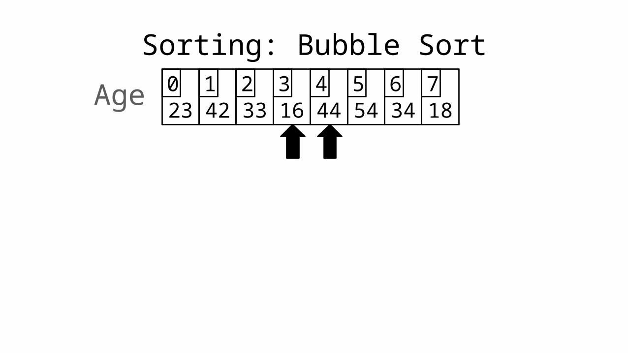
Sorting: Bubble Sort
44 23 42 33 16 54 34 180 1 2 3 4 5 6 7Age

Sorting: Bubble Sort
23 44 42 33 16 54 34 180 1 2 3 4 5 6 7Age

Sorting: Bubble Sort
23 44 42 33 16 54 34 180 1 2 3 4 5 6 7Age

Sorting: Bubble Sort
23 42 44 33 16 54 34 180 1 2 3 4 5 6 7Age

Sorting: Bubble Sort
23 42 44 33 16 54 34 180 1 2 3 4 5 6 7Age

Sorting: Bubble Sort
23 42 33 44 16 54 34 180 1 2 3 4 5 6 7Age

Sorting: Bubble Sort
23 42 33 44 16 54 34 180 1 2 3 4 5 6 7Age
Sorting: Bubble Sort
23 42 33 16 44 54 34 180 1 2 3 4 5 6 7Age

Sorting: Bubble Sort
23 42 33 16 44 54 34 180 1 2 3 4 5 6 7Age

Sorting: Bubble Sort
23 42 33 16 44 54 34 180 1 2 3 4 5 6 7Age

Sorting: Bubble Sort
23 42 33 16 44 54 34 180 1 2 3 4 5 6 7Age

Sorting: Bubble Sort
23 42 33 16 44 34 54 180 1 2 3 4 5 6 7Age
Sorting: Bubble Sort
23 42 33 16 44 34 54 180 1 2 3 4 5 6 7Age

Sorting: Bubble Sort
23 42 33 16 44 34 18 540 1 2 3 4 5 6 7Age
Sorting: Bubble Sort
23 42 33 16 44 34 18 540 1 2 3 4 5 6 7Age

Sorting: Bubble Sort
23 42 33 16 44 34 18 540 1 2 3 4 5 6 7Age
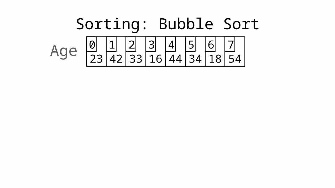
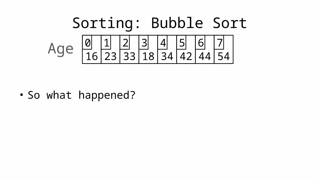
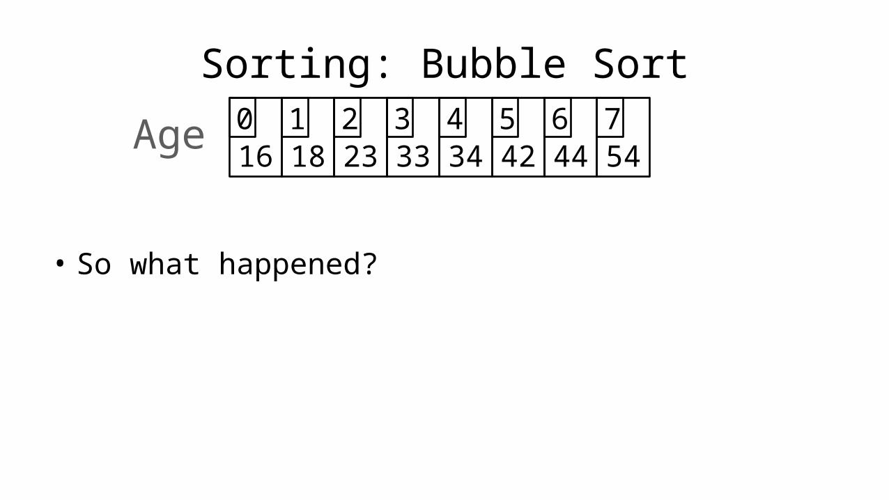
• So what happened?

Sorting: Bubble Sort
23 42 33 16 44 34 18 540 1 2 3 4 5 6 7Age
• So what happened?
• We have moved the largest value (54) into the correct position.

Sorting: Bubble Sort
• Let’s do it again:

Sorting: Bubble Sort
23 42 33 16 44 34 18 540 1 2 3 4 5 6 7Age

Sorting: Bubble Sort
42 23 33 16 44 34 18 540 1 2 3 4 5 6 7Age

Sorting: Bubble Sort
42 23 33 16 44 34 18 540 1 2 3 4 5 6 7Age

Sorting: Bubble Sort
42 23 33 16 44 34 18 540 1 2 3 4 5 6 7Age

Sorting: Bubble Sort
42 23 33 16 44 34 18 540 1 2 3 4 5 6 7Age

Sorting: Bubble Sort
42 23 16 33 44 34 18 540 1 2 3 4 5 6 7Age

Sorting: Bubble Sort
42 23 16 33 44 34 18 540 1 2 3 4 5 6 7Age

Sorting: Bubble Sort
42 23 16 33 44 34 18 540 1 2 3 4 5 6 7Age

Sorting: Bubble Sort
42 23 16 33 44 34 18 540 1 2 3 4 5 6 7Age

Sorting: Bubble Sort
42 23 16 33 34 44 18 540 1 2 3 4 5 6 7Age

Sorting: Bubble Sort
42 23 16 33 34 44 18 540 1 2 3 4 5 6 7Age

Sorting: Bubble Sort
42 23 16 33 34 18 44 540 1 2 3 4 5 6 7Age

Sorting: Bubble Sort
42 23 16 33 34 18 44 540 1 2 3 4 5 6 7Age

Sorting: Bubble Sort
42 23 16 33 34 18 44 540 1 2 3 4 5 6 7Age
• So what happened?

Sorting: Bubble Sort
42 23 16 33 34 18 44 540 1 2 3 4 5 6 7Age
• So what happened?
• We have moved the second largest value (44) into the correct position.

Sorting: Bubble Sort
• Let’s do it again:

Sorting: Bubble Sort
42 23 16 33 34 18 44 540 1 2 3 4 5 6 7Age

Sorting: Bubble Sort
23 42 16 33 34 18 44 540 1 2 3 4 5 6 7Age
Sorting: Bubble Sort
23 42 16 33 34 18 44 540 1 2 3 4 5 6 7Age

Sorting: Bubble Sort
23 16 42 33 34 18 44 540 1 2 3 4 5 6 7Age

Sorting: Bubble Sort
23 16 42 33 34 18 44 540 1 2 3 4 5 6 7Age
Sorting: Bubble Sort
23 16 42 33 34 18 44 540 1 2 3 4 5 6 7Age

Sorting: Bubble Sort
23 16 33 42 34 18 44 540 1 2 3 4 5 6 7Age

Sorting: Bubble Sort
23 16 33 42 34 18 44 540 1 2 3 4 5 6 7Age

Sorting: Bubble Sort
23 16 33 34 42 18 44 540 1 2 3 4 5 6 7Age

Sorting: Bubble Sort
23 16 33 34 42 18 44 540 1 2 3 4 5 6 7Age

Sorting: Bubble Sort
23 16 33 34 18 42 44 540 1 2 3 4 5 6 7Age

Sorting: Bubble Sort
23 16 33 34 18 42 44 540 1 2 3 4 5 6 7Age

Sorting: Bubble Sort
23 16 33 34 18 42 44 540 1 2 3 4 5 6 7Age

Sorting: Bubble Sort
23 16 33 34 18 42 44 540 1 2 3 4 5 6 7Age

Sorting: Bubble Sort
23 16 33 34 18 42 44 540 1 2 3 4 5 6 7Age
• So what happened?
• We have moved the third largest value (42) into the correct position.

Sorting: Bubble Sort
• Let’s do it again:

Sorting: Bubble Sort
23 16 33 34 18 42 44 540 1 2 3 4 5 6 7Age

Sorting: Bubble Sort
16 23 33 34 18 42 44 540 1 2 3 4 5 6 7Age

Sorting: Bubble Sort
16 23 33 34 18 42 44 540 1 2 3 4 5 6 7Age

Sorting: Bubble Sort
16 23 33 34 18 42 44 540 1 2 3 4 5 6 7Age

Sorting: Bubble Sort
16 23 33 34 18 42 44 540 1 2 3 4 5 6 7Age

Sorting: Bubble Sort
16 23 33 34 18 42 44 540 1 2 3 4 5 6 7Age

Sorting: Bubble Sort
16 23 33 34 18 42 44 540 1 2 3 4 5 6 7Age

Sorting: Bubble Sort
16 23 33 18 34 42 44 540 1 2 3 4 5 6 7Age

Sorting: Bubble Sort
16 23 33 18 34 42 44 540 1 2 3 4 5 6 7Age

Sorting: Bubble Sort
16 23 33 18 34 42 44 540 1 2 3 4 5 6 7Age

Sorting: Bubble Sort
16 23 33 18 34 42 44 540 1 2 3 4 5 6 7Age

Sorting: Bubble Sort
16 23 33 18 34 42 44 540 1 2 3 4 5 6 7Age

Sorting: Bubble Sort
16 23 33 18 34 42 44 540 1 2 3 4 5 6 7Age
Sorting: Bubble Sort
16 23 33 18 34 42 44 540 1 2 3 4 5 6 7Age
• So what happened?

Sorting: Bubble Sort
16 23 33 18 34 42 44 540 1 2 3 4 5 6 7Age
• So what happened?
• We have moved the fourth largest value (34) into the correct position.

Sorting: Bubble Sort
• Let’s do it again:

Sorting: Bubble Sort
16 23 33 18 34 42 44 540 1 2 3 4 5 6 7Age

Sorting: Bubble Sort
16 23 33 18 34 42 44 540 1 2 3 4 5 6 7Age

Sorting: Bubble Sort
16 23 33 18 34 42 44 540 1 2 3 4 5 6 7Age

Sorting: Bubble Sort
16 23 33 18 34 42 44 540 1 2 3 4 5 6 7Age

Sorting: Bubble Sort
16 23 33 18 34 42 44 540 1 2 3 4 5 6 7Age

Sorting: Bubble Sort
16 23 18 33 34 42 44 540 1 2 3 4 5 6 7Age

Sorting: Bubble Sort
16 23 18 33 34 42 44 540 1 2 3 4 5 6 7Age

Sorting: Bubble Sort
16 23 18 33 34 42 44 540 1 2 3 4 5 6 7Age

Sorting: Bubble Sort
16 23 18 33 34 42 44 540 1 2 3 4 5 6 7Age
Sorting: Bubble Sort
16 23 18 33 34 42 44 540 1 2 3 4 5 6 7Age

Sorting: Bubble Sort
16 23 18 33 34 42 44 540 1 2 3 4 5 6 7Age

Sorting: Bubble Sort
16 23 18 33 34 42 44 540 1 2 3 4 5 6 7Age

Sorting: Bubble Sort
16 23 18 33 34 42 44 540 1 2 3 4 5 6 7Age

Sorting: Bubble Sort
16 23 18 33 34 42 44 540 1 2 3 4 5 6 7Age
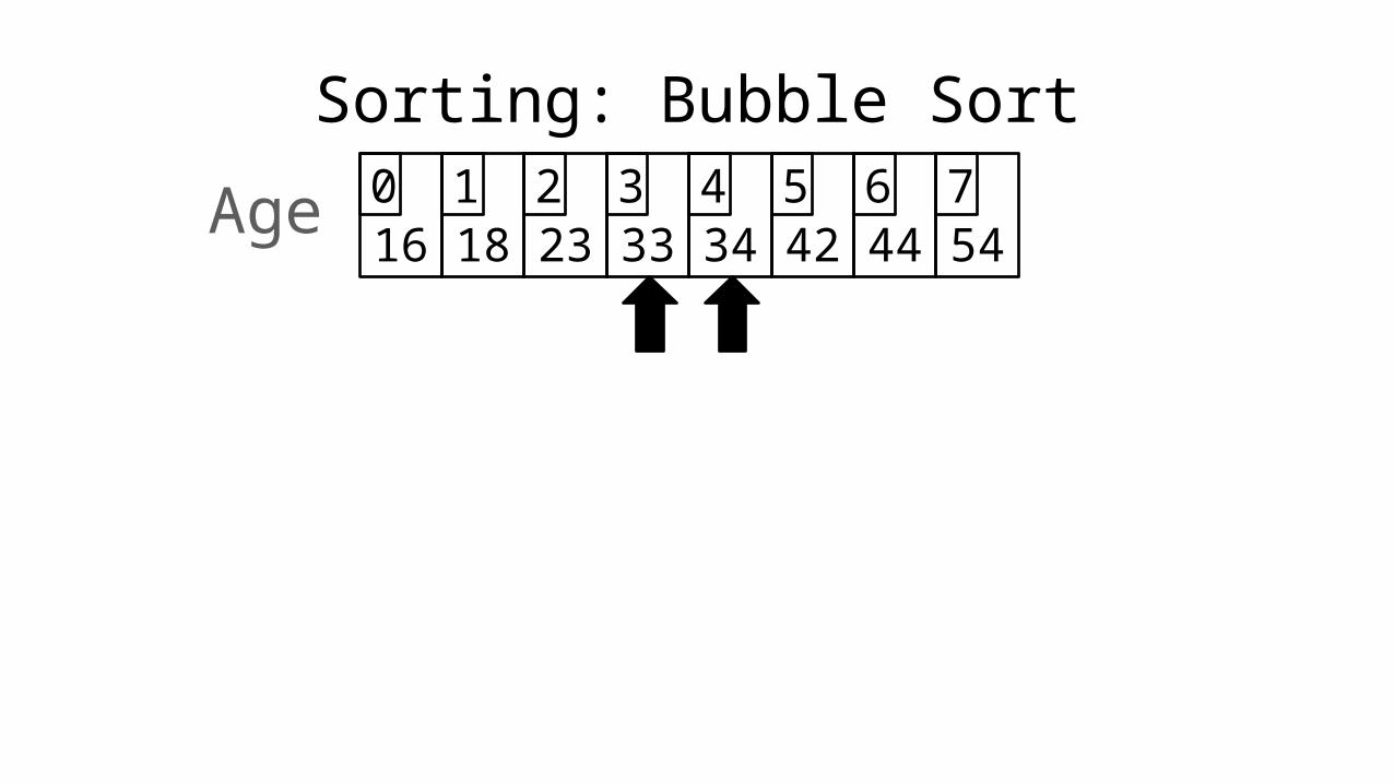
• So what happened?
• We have moved the fifth largest value (33) into the correct position.

Sorting: Bubble Sort
• Let’s do it again:

Sorting: Bubble Sort
16 23 18 33 34 42 44 540 1 2 3 4 5 6 7Age

Sorting: Bubble Sort
16 23 18 33 34 42 44 540 1 2 3 4 5 6 7Age

Sorting: Bubble Sort
16 23 18 33 34 42 44 540 1 2 3 4 5 6 7Age
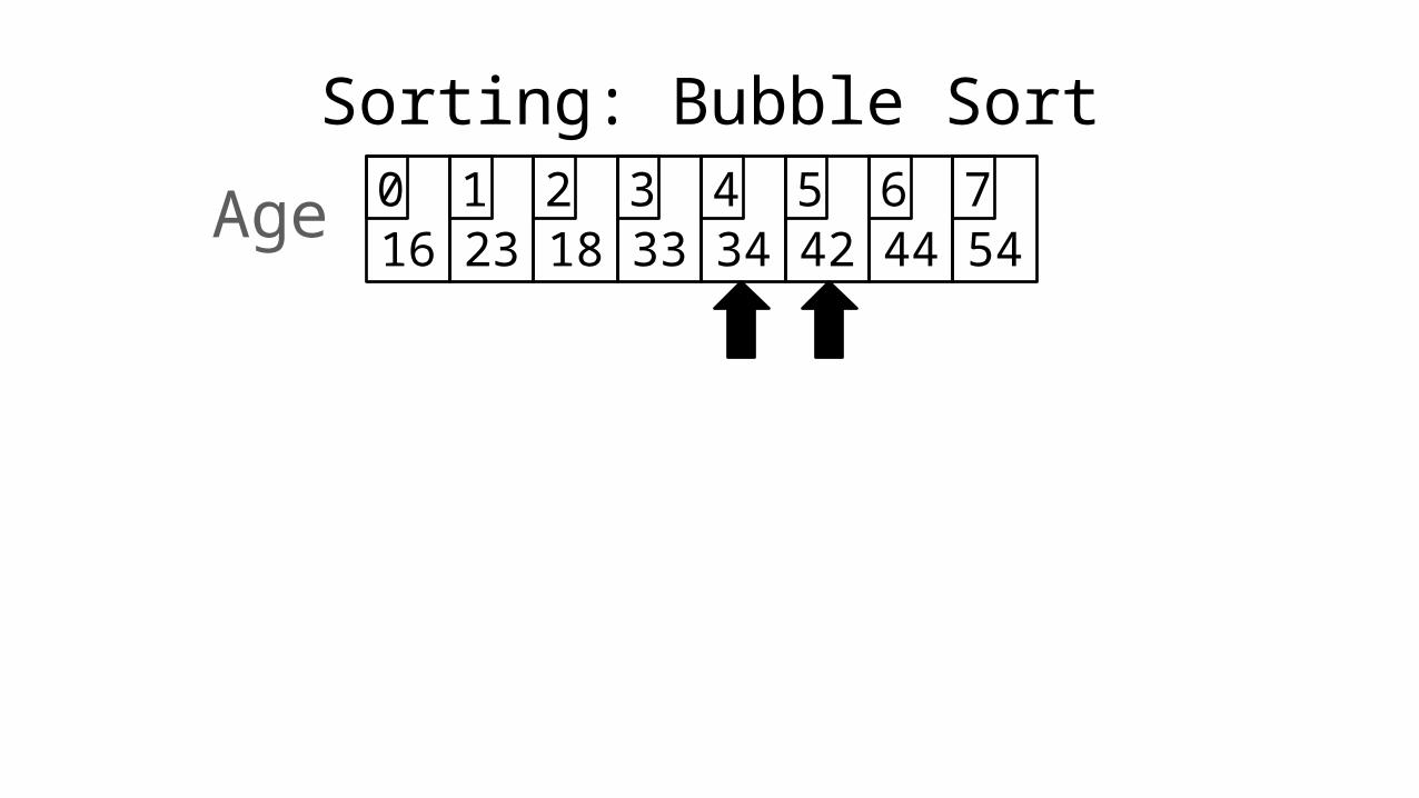
Sorting: Bubble Sort
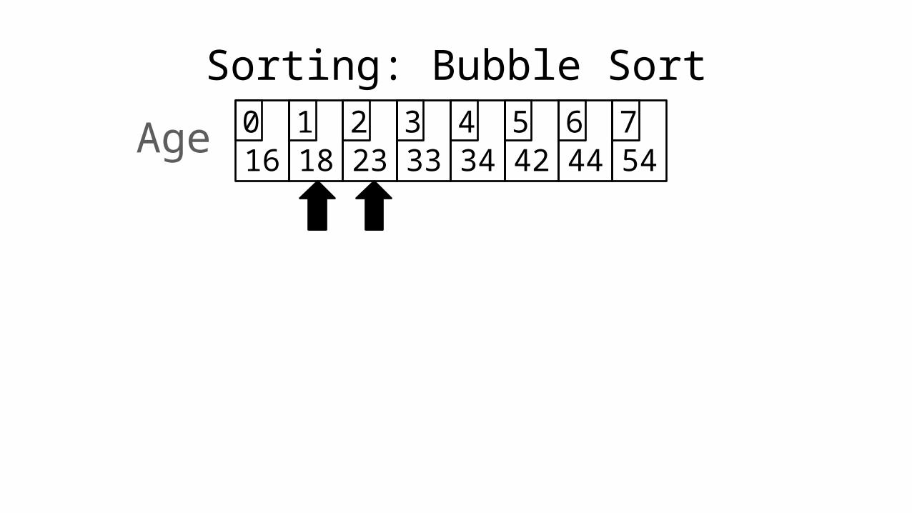
16 18 23 33 34 42 44 540 1 2 3 4 5 6 7Age

Sorting: Bubble Sort
16 18 23 33 34 42 44 540 1 2 3 4 5 6 7Age

Sorting: Bubble Sort
16 18 23 33 34 42 44 540 1 2 3 4 5 6 7Age

Sorting: Bubble Sort
16 18 23 33 34 42 44 540 1 2 3 4 5 6 7Age
Sorting: Bubble Sort
16 18 23 33 34 42 44 540 1 2 3 4 5 6 7Age

Sorting: Bubble Sort
16 18 23 33 34 42 44 540 1 2 3 4 5 6 7Age

Sorting: Bubble Sort
16 18 23 33 34 42 44 540 1 2 3 4 5 6 7Age

Sorting: Bubble Sort
16 18 23 33 34 42 44 540 1 2 3 4 5 6 7Age

Sorting: Bubble Sort
16 18 23 33 34 42 44 540 1 2 3 4 5 6 7Age

Sorting: Bubble Sort
16 18 23 33 34 42 44 540 1 2 3 4 5 6 7Age
Sorting: Bubble Sort
16 18 23 33 34 42 44 540 1 2 3 4 5 6 7Age
• So what happened?

Sorting: Bubble Sort
16 18 23 33 34 42 44 540 1 2 3 4 5 6 7Age
• So what happened?
• We have moved the sixth largest value (23) into the correct position.

Sorting: Bubble Sort
• Let’s do it again:

Sorting: Bubble Sort
• Let’s do it again:
• Let’s not bother!

Sorting: Bubble Sort
• Let’s do it again:
• Let’s not bother!
• It’s sorted!

Sorting: Bubble Sort
16 18 23 33 34 42 44 540 1 2 3 4 5 6 7Age

• So we need two loops:
Sorting: Bubble Sort

• So we need two loops:
FOR Outer-Index IN 0 TO N-1 FOR Index IN 0 TO N-2 DO IF (Age[Index+1] < Age[Index]) THEN Temp_Value <- Age[Index+1]; Age[Index+1] <- Age[Index]; Age[Index] <- Temp_Value; ENDIF; ENDFOR;
ENDFOR;
Sorting: Bubble Sort

PROGRAM BubbleSort: Integer Age[8] <- {44,23,42,33,16,54,34,18};
FOR Outer-Index IN 0 TO N-1 FOR Index IN 0 TO N-2 DO IF (Age[Index+1] < Age[Index]) THEN Temp_Value <- Age[Index+1]; Age[Index+1] <- Age[Index]; Age[Index] <- Temp_Value; ENDIF; ENDFOR;
ENDFOR;END.
Sorting: Bubble Sort

Sorting: Bubble Sort

Sorting:Optimising Bubblesort
Damian Gordon

Sorting: Bubble Sort
• If we look at the bubble sort algorithm again:

PROGRAM BubbleSort: Integer Age[8] <- {44,23,42,33,16,54,34,18};
FOR Outer-Index IN 0 TO N-1 FOR Index IN 0 TO N-2 DO IF (Age[Index+1] < Age[Index]) THEN Temp_Value <- Age[Index+1]; Age[Index+1] <- Age[Index]; Age[Index] <- Temp_Value; ENDIF; ENDFOR;
ENDFOR;END.
Sorting: Bubble Sort

Sorting: Bubble Sort
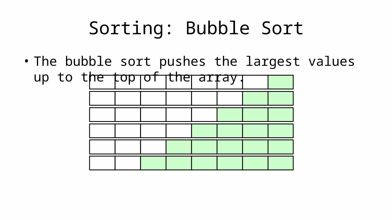
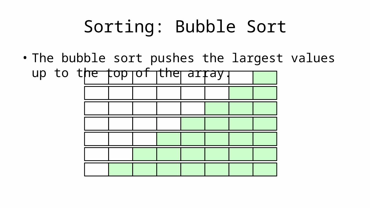
• The bubble sort pushes the largest values up to the top of the array.

Sorting: Bubble Sort
• The bubble sort pushes the largest values up to the top of the array.

Sorting: Bubble Sort
• The bubble sort pushes the largest values up to the top of the array.

Sorting: Bubble Sort
• The bubble sort pushes the largest values up to the top of the array.

Sorting: Bubble Sort
• The bubble sort pushes the largest values up to the top of the array.

Sorting: Bubble Sort
• The bubble sort pushes the largest values up to the top of the array.

Sorting: Bubble Sort
• The bubble sort pushes the largest values up to the top of the array.
Sorting: Bubble Sort
• The bubble sort pushes the largest values up to the top of the array.
Sorting: Bubble Sort
• The bubble sort pushes the largest values up to the top of the array.

Sorting: Bubble Sort
• The bubble sort pushes the largest values up to the top of the array.

Sorting: Bubble Sort
• So each time around the loop the amount of the array that is sorted is increased, and we don’t have to check for swaps in the locations that have already been sorted.
• So we reduce the checking of swaps by one each time we do a pass of the array.

Sorting: Bubble SortPROGRAM BubbleSort: Integer Age[8] <- {44,23,42,33,16,54,34,18};
ReducingIndex <- N-2;FOR Outer-Index IN 0 TO N-1 FOR Index IN 0 TO ReducingIndex DO IF (Age[Index+1] < Age[Index]) THEN Temp_Value <- Age[Index+1]; Age[Index+1] <- Age[Index]; Age[Index] <- Temp_Value; ENDIF; ENDFOR;ReducingIndex <- ReducingIndex – 1;
ENDFOR;END.

PROGRAM BubbleSort: Integer Age[8] <- {44,23,42,33,16,54,34,18};
ReducingIndex <- N-2;FOR Outer-Index IN 0 TO N-1 FOR Index IN 0 TO ReducingIndex DO IF (Age[Index+1] < Age[Index]) THEN Temp_Value <- Age[Index+1]; Age[Index+1] <- Age[Index]; Age[Index] <- Temp_Value; ENDIF; ENDFOR;ReducingIndex <- ReducingIndex – 1;
ENDFOR;END.
Sorting: Bubble Sort
Sorting: Bubble Sort
• Also, what if the data is already sorted?
• We should check if the program has done no swaps in one pass, and if t doesn’t that means the data is sorted.
• So even if the data started unsorted, as soon as the data gets sorted we want to exit the program.

Sorting: Bubble SortPROGRAM BubbleSort: Integer Age[8] <- {44,23,42,33,16,54,34,18};
ReducingIndex <- N-2;DidSwap <- FALSE;FOR Outer-Index IN 0 TO N-1 FOR Index IN 0 TO ReducingIndex DO IF (Age[Index+1] < Age[Index]) THEN Temp_Value <- Age[Index+1]; Age[Index+1] <- Age[Index]; Age[Index] <- Temp_Value; DidSwap <- TRUE; ENDIF; ENDFOR;ReducingIndex <- ReducingIndex – 1; IF (DidSwap = FALSE) THEN EXIT; ENDIF;
ENDFOR;END.

PROGRAM BubbleSort: Integer Age[8] <- {44,23,42,33,16,54,34,18};
ReducingIndex <- N-2;DidSwap <- FALSE;FOR Outer-Index IN 0 TO N-1 FOR Index IN 0 TO ReducingIndex DO IF (Age[Index+1] < Age[Index]) THEN Temp_Value <- Age[Index+1]; Age[Index+1] <- Age[Index]; Age[Index] <- Temp_Value; DidSwap <- TRUE; ENDIF; ENDFOR;ReducingIndex <- ReducingIndex – 1;IF (DidSwap = FALSE) THEN EXIT;ENDIF;
ENDFOR;END.
Sorting: Bubble Sort

Sorting: Bubble Sort
• The Swap function is very useful so we should have that as a method as follows:
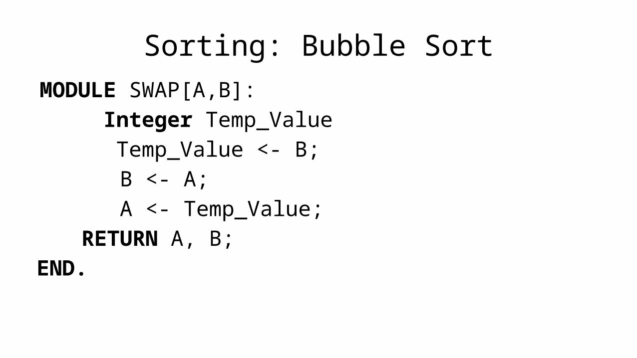
MODULE SWAP[A,B]: Integer Temp_Value Temp_Value <- B;
B <- A; A <- Temp_Value;RETURN A, B;
END.
Sorting: Bubble Sort

PROGRAM BubbleSort: Integer Age[8] <- {44,23,42,33,16,54,34,18};
ReducingIndex <- N-2;DidSwap <- FALSE;FOR Outer-Index IN 0 TO N-1 FOR Index IN 0 TO ReducingIndex DO IF (Age[Index+1] < Age[Index]) THEN Temp_Value <- Age[Index+1]; Age[Index+1] <- Age[Index]; Age[Index] <- Temp_Value; DidSwap <- TRUE; ENDIF; ENDFOR;ReducingIndex <- ReducingIndex – 1;IF (DidSwap = FALSE) THEN EXIT;ENDIF;
ENDFOR;END.
Sorting: Bubble Sort

PROGRAM BubbleSort: Integer Age[8] <- {44,23,42,33,16,54,34,18};
ReducingIndex <- N-2;DidSwap <- FALSE;FOR Outer-Index IN 0 TO N-1 FOR Index IN 0 TO ReducingIndex DO IF (Age[Index+1] < Age[Index]) THEN SWAP(Age[Index], Age[Index+1]; DidSwap <- TRUE; ENDIF; ENDFOR;ReducingIndex <- ReducingIndex – 1;IF (DidSwap = FALSE) THEN EXIT;ENDIF;
ENDFOR;END.
Sorting: Bubble Sort

Sorting:Selection Sort
Damian Gordon

Sorting: Selection Sort
• OK, so we’ve seen a way of sorting that easy for the computer, now let’s look at a ways that’s more natural for a person to understand.
• It’s called selection sort.

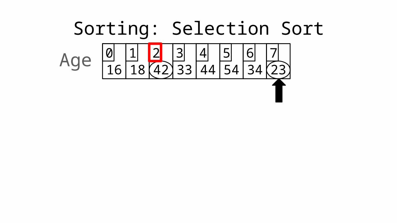
Sorting: Selection Sort
• It works as follows:– Find the smallest number, swap it with the value in the first location
of the array– Find the second smallest number, swap it with the value in the
second location of the array– Find the third smallest number, swap it with the value in the third
location of the array– Etc.

Sorting: Selection Sort
44 23 42 33 16 54 34 180 1 2 3 4 5 6 7Age

Sorting: Selection Sort
44 23 42 33 16 54 34 180 1 2 3 4 5 6 7Age

Sorting: Selection Sort
44 23 42 33 16 54 34 180 1 2 3 4 5 6 7Age

Sorting: Selection Sort
16 23 42 33 44 54 34 180 1 2 3 4 5 6 7Age

Sorting: Selection Sort
16 23 42 33 44 54 34 180 1 2 3 4 5 6 7Age

Sorting: Selection Sort
16 23 42 33 44 54 34 180 1 2 3 4 5 6 7Age

Sorting: Selection Sort
16 18 42 33 44 54 34 230 1 2 3 4 5 6 7Age

Sorting: Selection Sort
16 18 42 33 44 54 34 230 1 2 3 4 5 6 7Age
Sorting: Selection Sort
16 18 42 33 44 54 34 230 1 2 3 4 5 6 7Age

Sorting: Selection Sort
16 18 23 33 44 54 34 420 1 2 3 4 5 6 7Age

Sorting: Selection Sort
16 18 23 33 44 54 34 420 1 2 3 4 5 6 7Age

Sorting: Selection Sort
16 18 23 33 44 54 34 420 1 2 3 4 5 6 7Age

Sorting: Selection Sort
16 18 23 33 44 54 34 420 1 2 3 4 5 6 7Age

Sorting: Selection Sort
16 18 23 33 44 54 34 420 1 2 3 4 5 6 7Age

Sorting: Selection Sort
16 18 23 33 34 54 44 420 1 2 3 4 5 6 7Age

Sorting: Selection Sort
16 18 23 33 34 54 44 420 1 2 3 4 5 6 7Age

Sorting: Selection Sort
16 18 23 33 34 54 44 420 1 2 3 4 5 6 7Age

Sorting: Selection Sort
16 18 23 33 34 42 44 540 1 2 3 4 5 6 7Age

Sorting: Selection Sort
16 18 23 33 34 42 44 540 1 2 3 4 5 6 7Age

Sorting: Selection Sort
16 18 23 33 34 42 44 540 1 2 3 4 5 6 7Age

Sorting: Selection Sort
16 18 23 33 34 42 44 540 1 2 3 4 5 6 7Age

Sorting: Selection Sort
16 18 23 33 34 42 44 540 1 2 3 4 5 6 7Age

Sorting: Selection Sort
• So we know we only have to swap if the value is not already in the correct location.

Sorting: Selection Sort
• So we know we only have to swap if the value is not already in the correct location.
• This will look a little something like this:
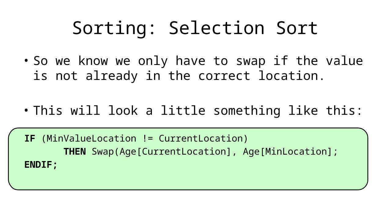
Sorting: Selection Sort
• So we know we only have to swap if the value is not already in the correct location.
• This will look a little something like this:
IF (MinValueLocation != CurrentLocation) THEN Swap(Age[CurrentLocation], Age[MinLocation];ENDIF;

• We will find the minimum value in the list using something like the following:
MinLocation <- 0; FOR Index IN IncreasingCount TO N-1 DO IF (Age[Index] < Age[MinValueLocation]) THEN MinLocation <- Index; ENDIF; ENDFOR;
Sorting: Selection Sort

Sorting: Selection Sort
• So we can put these two bits together,

PROGRAM SelectionSort: Integer Age[8] <- {44,23,42,33,16,54,34,18};
FOR Outer-Index IN 0 TO N-1 MinValueLocation <- Outer-Index; FOR Index IN Outer-Index+1 TO N-1 DO IF (Age[Index] < Age[MinValueLocation]) THEN MinLocation <- Index; ENDIF; ENDFOR; IF (MinValueLocation != Outer-Index) THEN Swap(Age[Outer-Index], Age[MinValueLocation]); ENDIF;
ENDFOR;END.
Sorting: Selection Sort

Sorting: Selection Sort

Data Structures:Multi-Dimensional Arrays
Damian Gordon

Arrays
• We declare a multi-dimensional array as follows:• Integer Age[8][8];

Arrays
Matrix
(0,0)
(1,0)
(2,0)
(3,0)
(4,0)
(5,0)
(6,0)
(7,0)
(0,1)
(1,1)
(2,1)
(3,1)
(4,1)
(5,1)
(6,1)
(7,1)
(0,2)
(1,2)
(2,2)
(3,2)
(4,2)
(5,2)
(6,2)
(7,2)
(0,3)
(1,3)
(2,3)
(3,3)
(4,3)
(5,3)
(6,3)
(7,3)
(0,4)
(1,4)
(2,4)
(3,4)
(4,4)
(5,4)
(6,4)
(7,4)
(0,5)
(1,5)
(2,5)
(3,5)
(4,5)
(5,5)
(6,5)
(7,5)
(0,6)
(1,6)
(2,6)
(3,6)
(4,6)
(5,6)
(6,6)
(7,6)
(0,7)
(1,7)
(2,7)
(3,7)
(4,7)
(5,7)
(6,7)
(7,7)

Arrays
Matrix
45
23
55
123
304
27
79
33
67
57
345
90
63
29
46
30
34
37
31
34
39
78
30
63
256
36
86
56
32
80
27
20
77
84
36
90
12
67
65
244
64
92
15
14
3
66
467
25
632
17
203
31
415
267
87
53
31
88
7
6
56
655
99
23

Arrays

Arrays

Arrays
• So if I do:• PRINT Matrix[0][0];
• We will get:• 45

Arrays
• So if I do:• PRINT Matrix[2][0];
• We will get:• 55

Arrays
• So if I do:• PRINT Matrix[0][2];
• We will get:• 34

Arrays
• So if I do:• PRINT Matrix[7][7];
• We will get:• 23

Arrays
• So if I do:• Matrix[5][4] <- 43;
• We will get:• 67 changed to 43
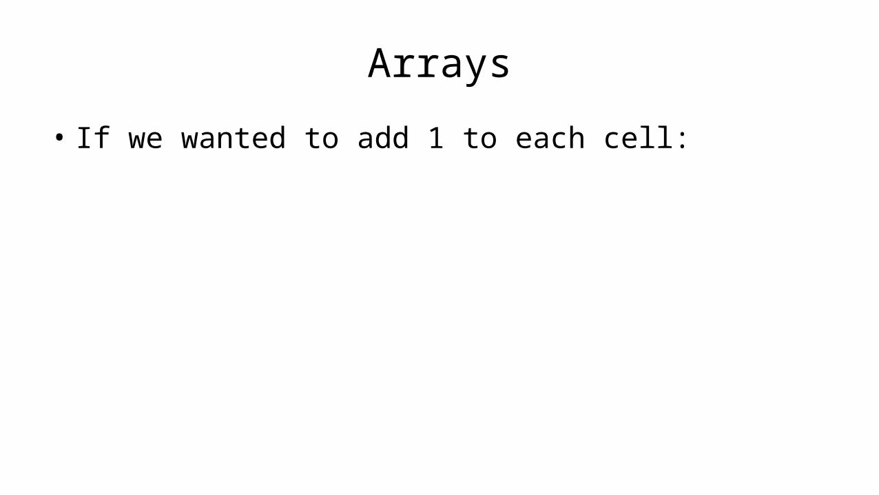
Arrays
• If we wanted to add 1 to each cell:

Arrays
PROGRAM Add1ToMartix: FOR N IN 0 TO 7 FOR M IN 0 TO 7 DO Matrix[N][M] <- Matrix [N][M] + 1; ENDFOR; ENDFOR;END.

Arrays
Or:
PROGRAM Add1ToMartix: FOR ROW IN 0 TO 7 FOR COLUMN IN 0 TO 7 DO Matrix[ROW][COLUMN] <- Matrix [ROW][COLUMN] + 1; ENDFOR; ENDFOR;END.
Arrays
• If we want to add up all the values in the array:

Arrays
PROGRAM TotalOfMatrix: integer Total <- 0; FOR N IN 0 TO 7 FOR M IN 0 TO 7 DO Total <- Total + Matrix[N][M]; ENDFOR; ENDFOR;END.

Arrays
• If we want to add up all the values in the array:
PROGRAM TotalOfMatrix: integer Total <- 0; FOR N IN 0 TO 39 DO Total <- Total + Age[N]; ENDFOR;END.

Arrays
• We can also have a multi-dimensional array of characters.• We can also have a multi-dimensional array of reals.• We can also have a multi-dimensional array of strings.• We can also have a multi-dimensional array of booleans.

Arrays
• We can create a 3D array: Array[N][N][N]• We can create a 4D array: Array[N][N][N][N]• We can create a 5D array: Array[N][N][N][N][N]• etc.

Data Structures:Advanced
Damian Gordon

Advanced Data Structure
• We’ll look at:– Linked Lists– Trees– Stacks– Queues

Linked Lists
• Imagine we wanted to have an array where we can dynamically add elements into it, and take them away.
• We can do this with a linked list.

Linked Lists
• A linked list is made up of nodes.

Linked Lists
• A linked list is made up of nodes.
• Each node has two parts to it:

Linked Lists
• A linked list is made up of nodes.
• Each node has two parts to it:
PointerValue

Linked Lists
• For example

Linked Lists
• For example
23

Linked Lists
• For example
23 62

Linked Lists
• For example
23 62 37

Linked Lists
• For example
23 62 37 31

Linked Lists
• For example
23 62 37 31 NULL

Linked Lists
• For example
23 62 37 31 NULL
Startof List
Endof List

Linked Lists
• To add a value in:
23 62 37 31 NULL
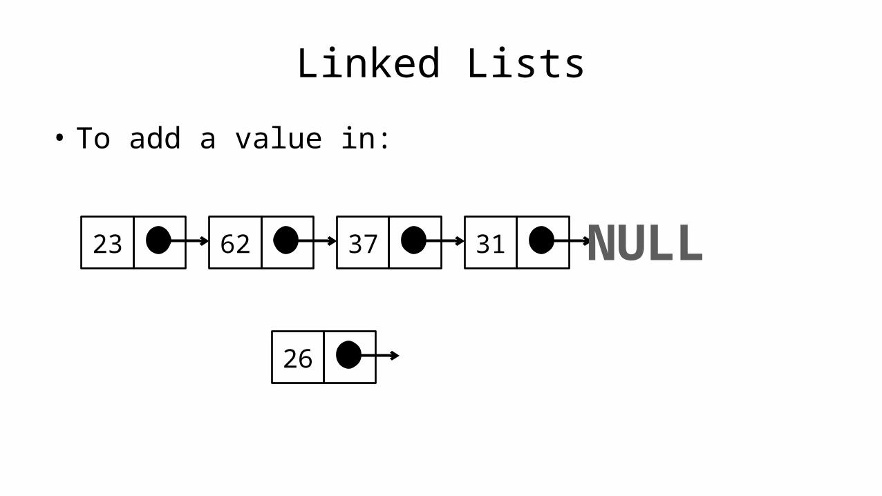
Linked Lists
• To add a value in:
23 62 37 31 NULL
26

Linked Lists
• To add a value in:
23 62 37 31 NULL
26

Linked Lists
• To add a value in:
23 62 37 31 NULL
26
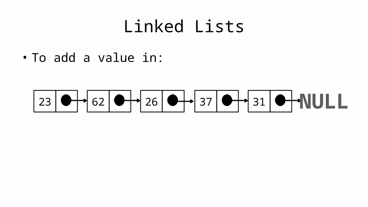
Linked Lists
• To add a value in:
23 62 37 31 NULL26

Linked Lists
• To delete a value:
23 62 37 31 NULL26

Linked Lists
• To delete a value:
23 62 37 31 NULL26

Linked Lists
• To delete a value:
23 62 37 31 NULL

Trees
• We can also have a tree:

Trees
• We can also have a tree:
• A tree is made up of nodes.
• Each node has three parts.

Trees
• We can also have a tree:
• A tree is made up of nodes.
• Each node has three parts.
• A value and two pointers, a left and a right one.
Value
RightLeft

Trees
• This is what it looks like:
23
68 14
33 831153
77 27

Trees
• This is what it looks like:
23
68 14
33 831153
Root
Parent
Child
77Leaf 27
Stacks
• We can also have a stack:

Stacks
• We can also have a stack:

Stacks
• We can also have a stack:
• It’s a structure that conforms to the principle of Last In, First Out (LIFO).
• The last item to join the stack is the first item to be served.

Stacks
314159265359

Stacks
314159265359 Top
Bottom
Stacks
• Values are added to the top:

Stacks
• Values are added to the top:
314159265359
67
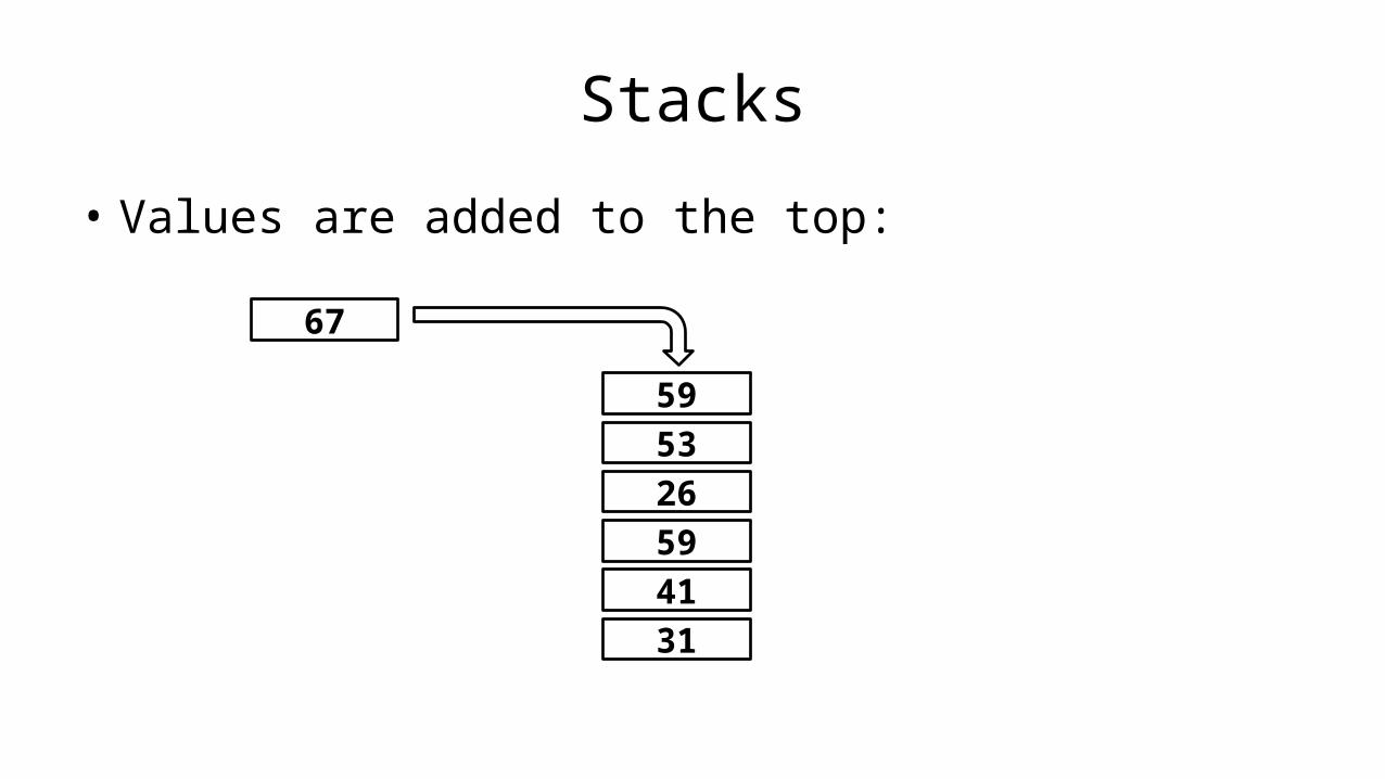
Stacks
• Values are added to the top:
314159265359
67

Stacks
• Values are added to the top:
314159265359
67

Stacks
• Values are removed from the top:
314159265359
67
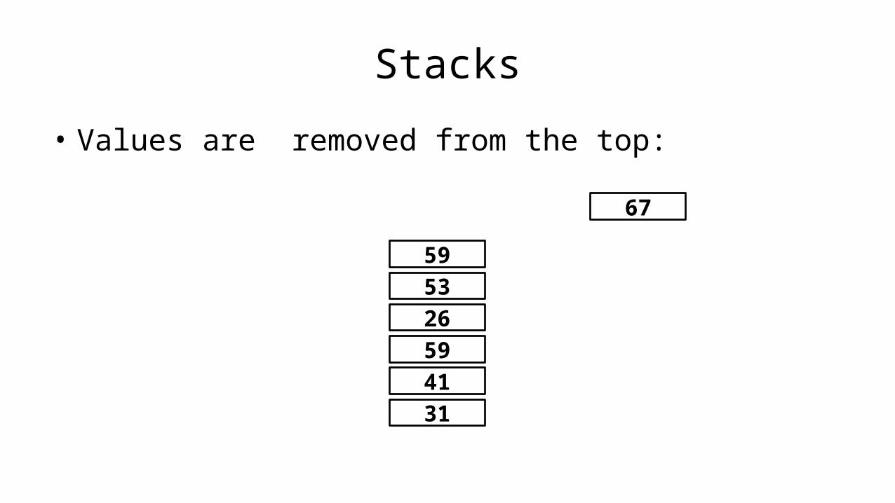
Stacks
• Values are removed from the top:
314159265359
67
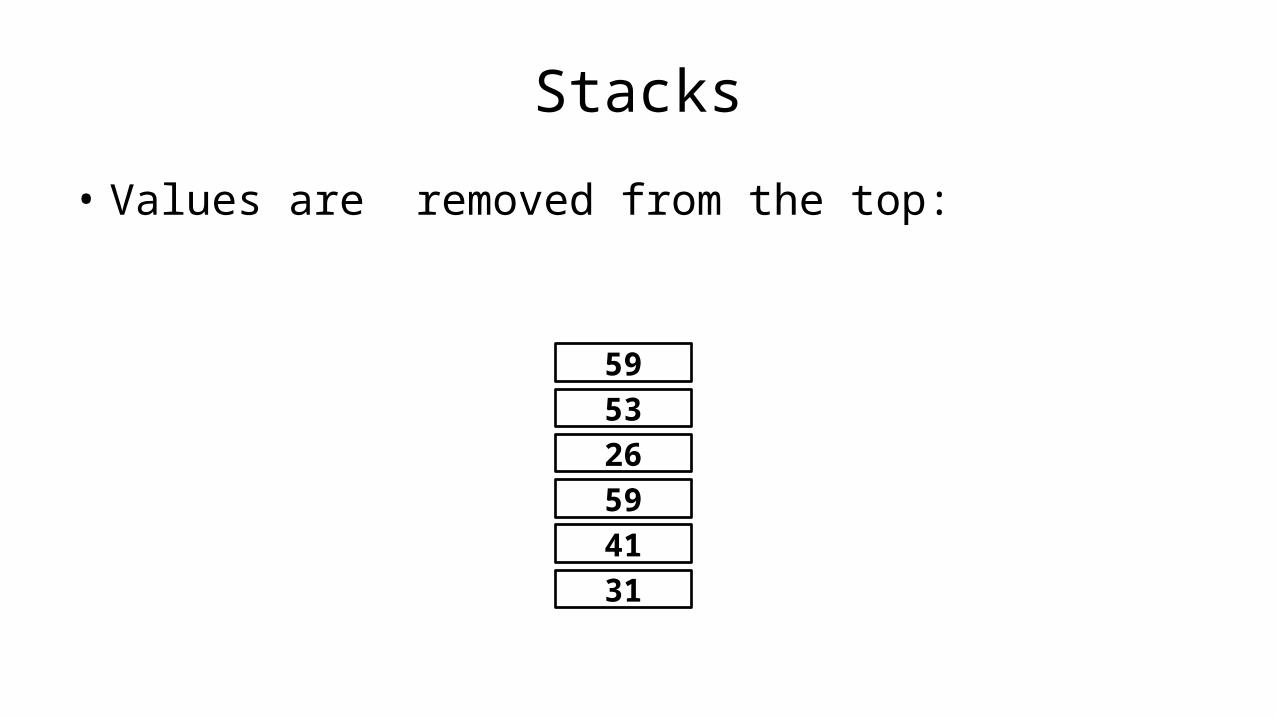
Stacks
• Values are removed from the top:
314159265359

Queues
• We can also have a queue:

Queues
• We can also have a queue:

Queues
• We can also have a queue:
• It’s a structure that conforms to the principle of First In, First Out (FIFO).
• The first item to join the queue is the first item to be served.

Queues
314159265359

Queues
314159265359
Back Front

Queues
• Values are added to the back:
314159265359
86

Queues
• Values are added to the back:
314159265359
86

Queues
• Values are added to the back:
31415926535986

Queues
• Values are removed from the front:
31415926535986
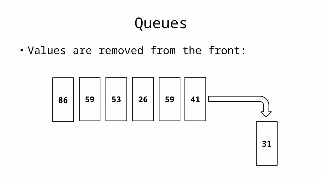
Queues
• Values are removed from the front:
31
415926535986

Queues
• Values are removed from the front:
31
415926535986

Queues
• Values are removed from the front:
415926535986

Technical Architectures
Damian Gordon

Contents
• 2-Tier Architecture (Client/Server)• 3-Tier Architecture• N-Tier Architecture• N-Tier Architecture (with Server Load Balancing)
http://cis.cuyamaca.net/draney/214/web_server/client.htm

2-Tier Architecture (Client/Server)


Most Processing happens here!

Most Processing happens here!
Most Processing happens here!

3-Tier Architecture


N-Tier Architecture


N-Tier Architecture with Server Load Balancing


SoftwareDevelopment
Methodologies
Damian Gordon

Timeline of Methodologies
1950s Code & Fix1960s Design-Code-Test-Maintain1970s Waterfall Model1980s Spiral Model1990s V-Model/Rapid Application Development2000s Agile Methods

1950s: Code & Fix

Code-and-Fix
• Aka “Code-like-Hell”–Specification (maybe), –Code (yes), –Release (maybe)
• Suitable for prototypes or throwaways
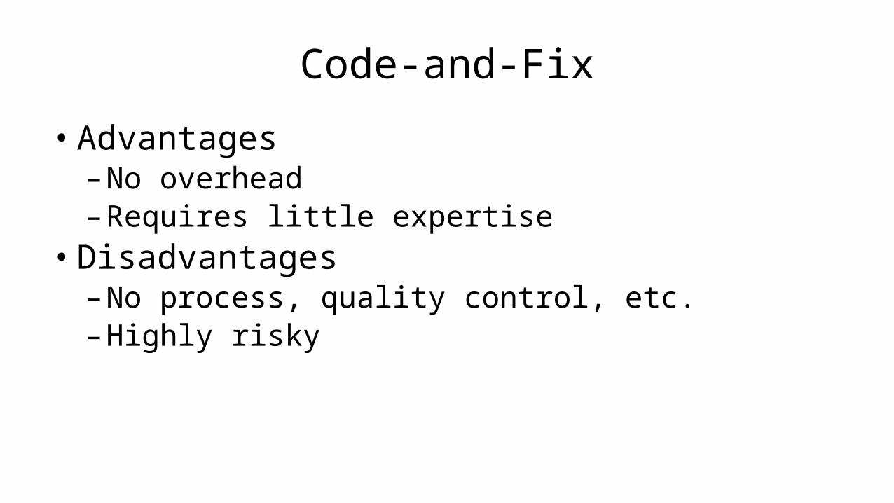
Code-and-Fix
• Advantages–No overhead–Requires little expertise
• Disadvantages–No process, quality control, etc.–Highly risky
1960s: Design-Code-Test-Maintain

Design-Code-Test-Maintain
• Design: – Specify requirement diagrammatically
• Code: – Write the code
• Test: – Check if it is working
• Maintain: – Keep it up-to-date

• Advantages–More process control– Less risky
• Disadvantages–More Overhead–Requires more expretise
Design-Code-Test-Maintain

1970s: Waterfall Model

Managing the Development of Large Software Systems
by W.W. Royce
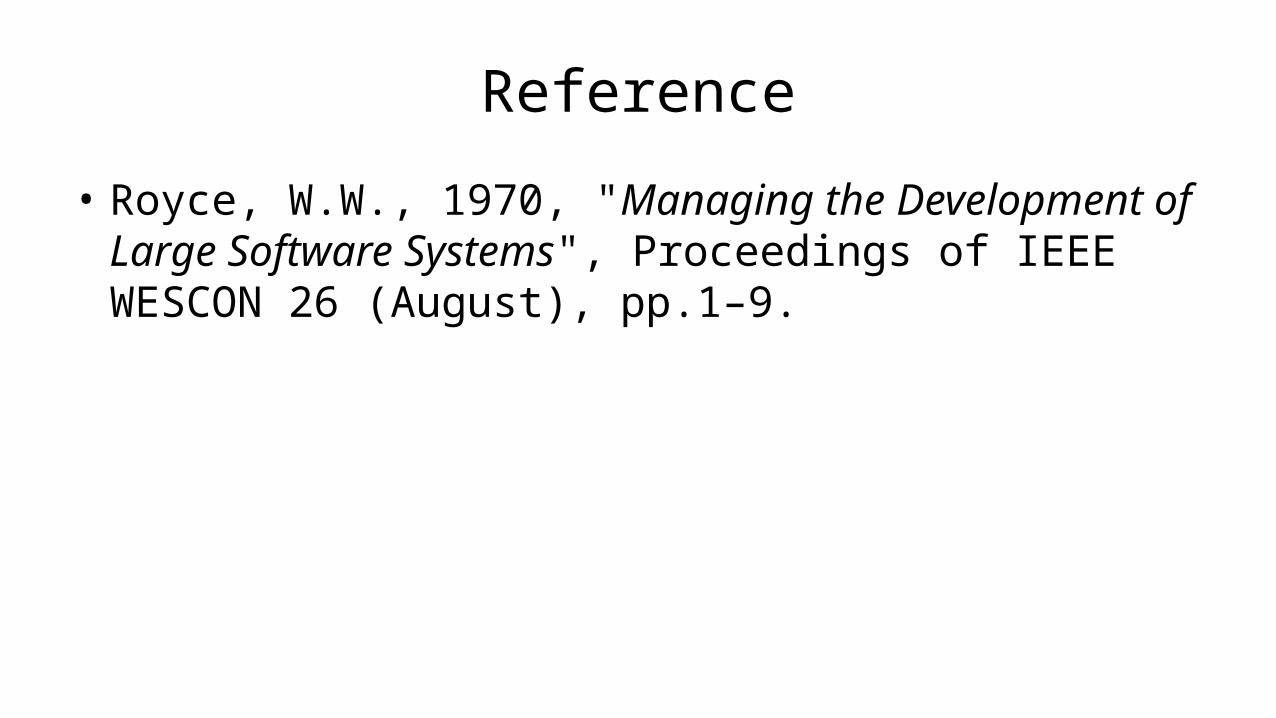
Reference
• Royce, W.W., 1970, "Managing the Development of Large Software Systems", Proceedings of IEEE WESCON 26 (August), pp.1–9.

Winston W. Royce• Born in 1929.• Died in 1995.• An American computer scientist, director
at Lockheed Software Technology Center in Austin, Texas, and one of the leaders in software development in the second half of the 20th century.
• He was the first person to describe the “Waterfall model” for software development, although Royce did not use the term "waterfall" in that article, nor advocated the waterfall model as a working methodology.

Introduction
• “I am going to describe my personal views about managing large software developments.
• I have had various assignments during the past nine years, mostly concerned with the development of software packages for spacecraft mission planning, commanding and post-flight analysis.
• In these assignments I have experienced different degrees of success with respect to arriving at an operational state, on-time, and within costs.
• I have become prejudiced by my experiences and I am going to relate some of these prejudices in this presentation.”

Small Developments
• For a small development, you only need the following steps– Typically done for programs for internal use

Large Developments

Large Developments
• System Requirements: Identify, select and document functional, scheduling and financial requirements.

Large Developments
• Software Requirements: Identify, select and document the software features necessary to satisfy the system requirements.

Large Developments
• Analysis: Methodically work through the details of each requirement.

Large Developments
• Program Design: Use programming techniques to design software and hardware within the constraints and objectives set in the earlier stages.

Large Developments
• Coding: Implement the program as designed in the earlier stages.

Large Developments
• Testing: Test the software and record the results.

Large Developments
• Operations: Deliver, install and configure the completed software.

Large Developments

Large Developments
"I believe in this concept, but the implementation described above is risky
and invites failure."

Iterative Relationship between Successive Development Phases

Iterative Relationship between Successive Development Phases
• Each step progresses and the design is further detailed, there is an iteration with the preceding and succeeding steps but rarely with the more remote steps in the sequence.
• The virtue of all of this is that as the design proceeds the change process is scoped down to manageable limits.

Unfortunately the design iterations are never confined to the successive steps

Unfortunately the design iterations are never confined to the successive steps
• The testing phase which occurs at the end of the development cycle is the first event for which timing, storage, input/output transfers, etc., are experienced as distinguished from analyzed.
• These phenomena are not precisely analyzable. • Yet if these phenomena fail to satisfy the various external
constraints, then invariably a major redesign is required.

How do we fix this?

Five Steps
1. Program Design comes first2. Document the Design3. Do it twice4. Plan, Control and Monitor Testing5. Involve the Customer

1. Program Design comes first
• A preliminary program design phase has been inserted between the Software Requirements Generation phase and the Analysis phase.

1. Program Design comes first
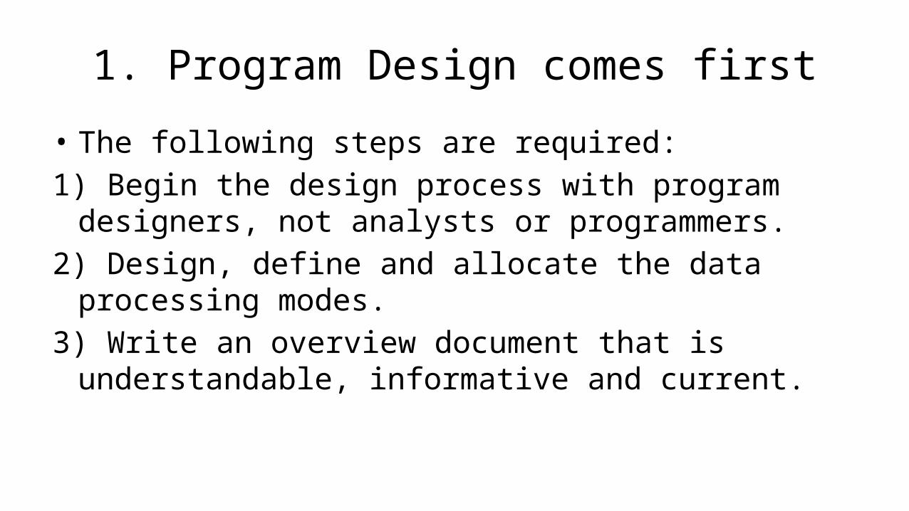
1. Program Design comes first
• The following steps are required:1) Begin the design process with program designers, not analysts
or programmers.2) Design, define and allocate the data processing modes. 3) Write an overview document that is understandable,
informative and current.
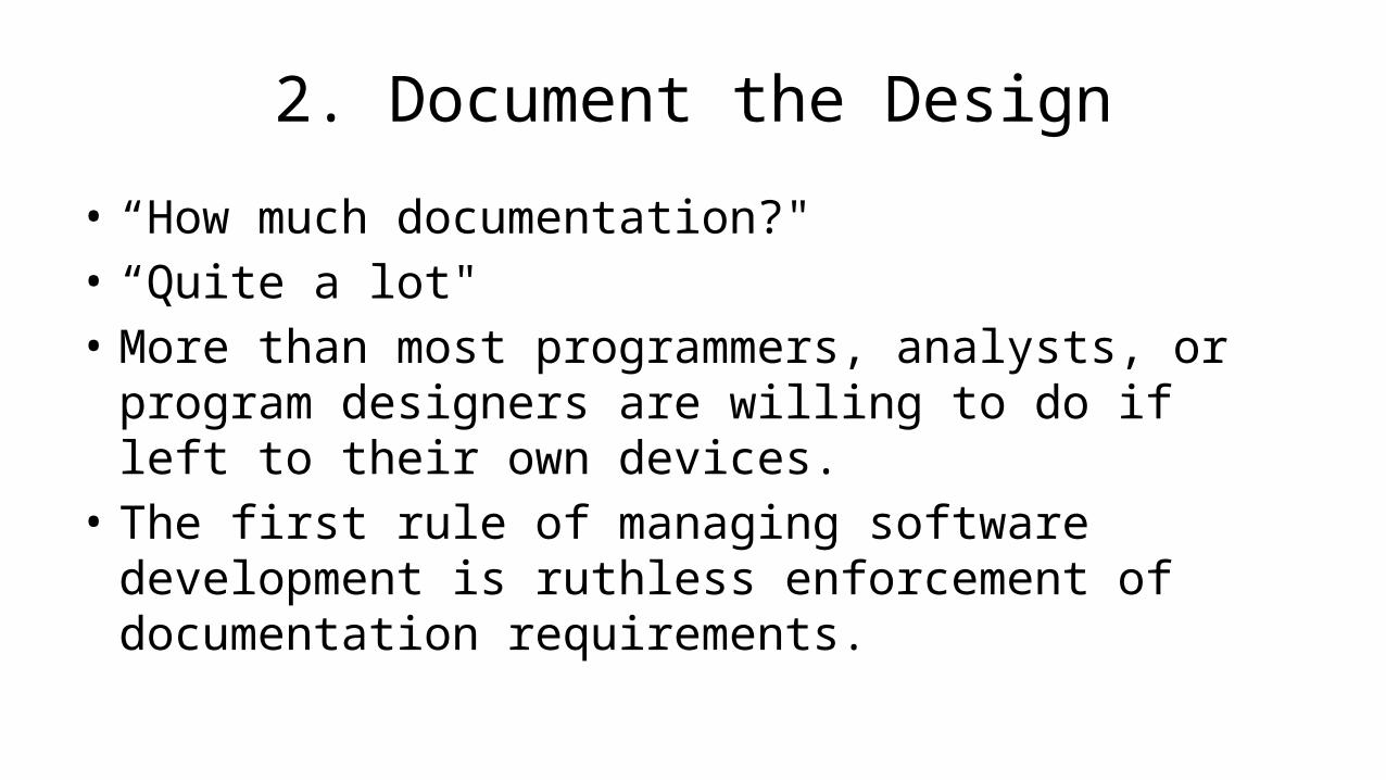
2. Document the Design
• “How much documentation?" • “Quite a lot" • More than most programmers, analysts, or program designers
are willing to do if left to their own devices. • The first rule of managing software development is ruthless
enforcement of documentation requirements.

2. Document the Design

3. Do It Twice
• Create a pilot study• If the computer program in question is being developed for the
first time, arrange matters so that the version finally delivered to the customer for operational deployment is actually the second version insofar as critical design/operations areas are concerned.
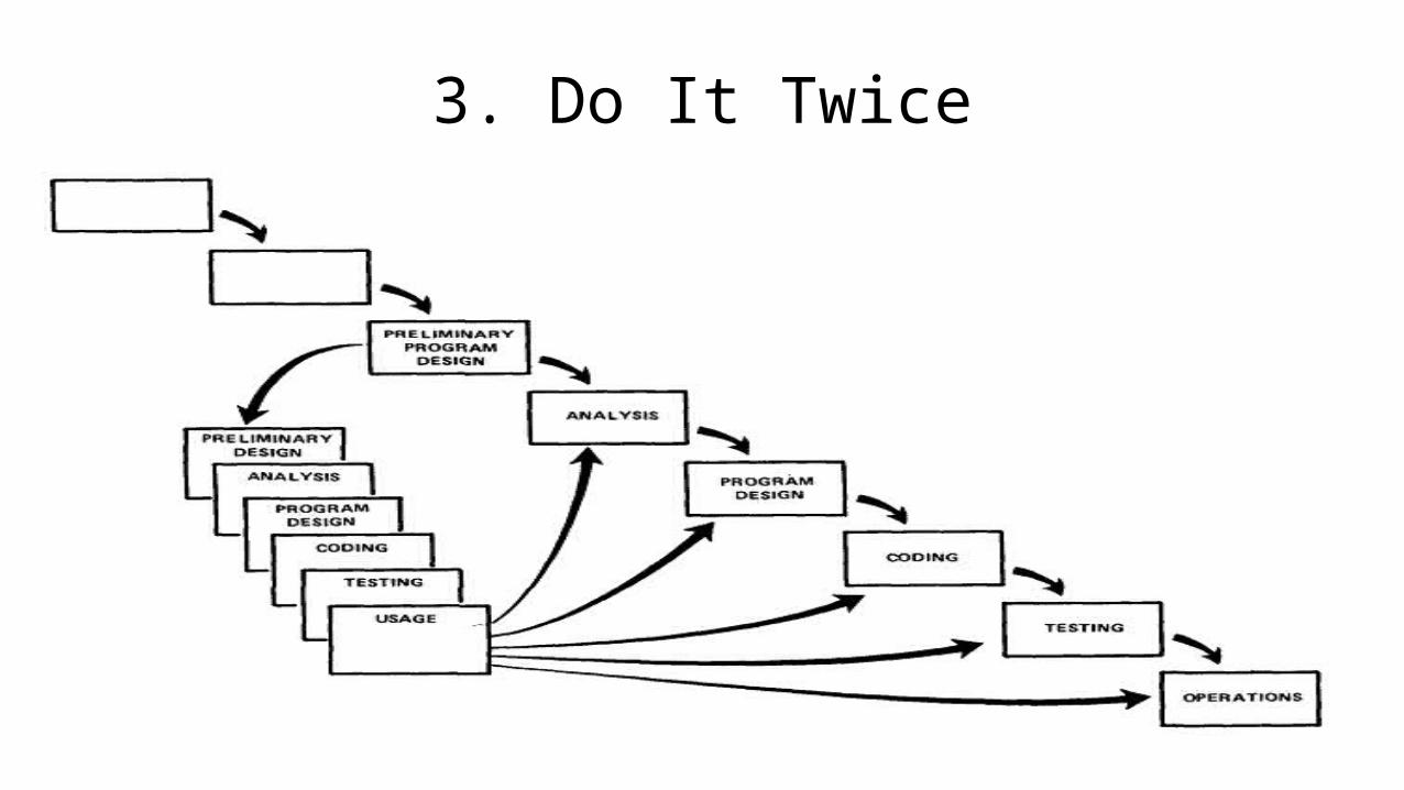
3. Do It Twice

4. Plan, Control and Monitor Testing
• Without question the biggest user of project resources, whether it be manpower, computer time, or management judgment, is the test phase. It is the phase of greatest risk in terms of dollars and schedule.

4. Plan, Control and Monitor Testing

4. Plan, Control and Monitor Testing
1) Many parts of the test process are best handled by test specialists who did not necessarily contribute to the original design.
2) Most errors are of an obvious nature that can be easily spotted by visual inspection.
3) Test every logic path in the computer program at least once with some kind of numerical check.
4) After the simple errors (which are in the majority, and which obscure the big mistakes) are removed, then it is time to turn over the software to the test area for checkout purposes.

5. Involve the Customer
• For some reason what a software design is going to do is subject to wide interpretation even after previous agreement.
• It is important to involve the customer in a formal way so that he has committed himself at earlier points before final delivery.
• To give the contractor free rein between requirement definition and operation is inviting trouble.

5. Involve the Customer

Summary

1980s: Spiral Model

A Spiral Model of Software Development and Enhancementby
Barry Boehm

Reference
• Boehm, B., 1986, "A Spiral Model of Software Development and Enhancement", ACM SIGSOFT Software Engineering Notes, 11(4) (August), pp.14-24.

Barry Boehm
• Born in 1935.• An American software engineer,
TRW Emeritus Professor of Software Engineering at the Computer Science Department of the University of Southern California.
• Known for his many contributions to software engineering.

Introduction• “These statements exemplify the current debate about software life-cycle process models. The topic has recently
received a great deal of attention.• The Defense Science Board Task Force Report on Military Software issued in 1987 highlighted the concern that
traditional software process models were discouraging more effective approaches to software development such as prototyping and software reuse. The Computer Society has sponsored tutorials and workshops on software process models that have helped clarify many of the issues and stimulated advances in the field (see “Further Reading”).
• The spiral model presented in this article is one candidate for improving the software process model situation. The major distinguishing feature of the spiral model is that it creates a risk-driven approach to the software process rather than a primarily document-driven or code-driven process. It incorporates many of the strengths of other models and resolves many of their difficulties.
• This article opens with a short description of software process models and the issues they address. Subsequent sections outline the process steps involved in the spiral model; illustrate the application of the spiral model to a software project, using the TRW Software Productivity Project as an example; summarize the primary advantages and implications involved in using the spiral model and the primary difficulties in using it at its current incomplete level of elaboration; and present resulting conclusions.”
“Stop the life cycle—I want to get off!”“Life-cycle Concept Considered Harmful.”“ The waterfall model is dead.”“No, it isn’t, but it should be.”

Background
• The primary functions of a software process model are to determine the order of the stages involved in software development and evolution and to establish the transition criteria for progressing from one stage to the next.

Background
• Thus the key questions that a process model must consider are:
1) What shall we do next?2) How long shall we continue to do it?
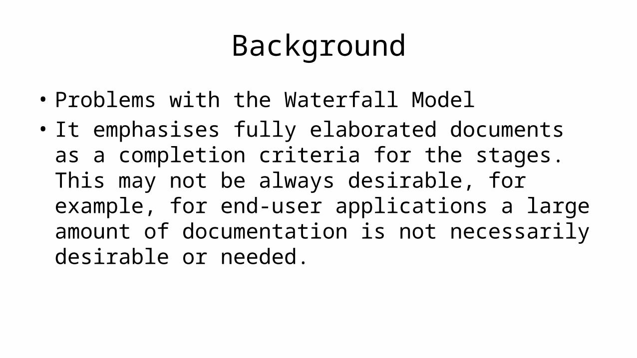
Background
• Problems with the Waterfall Model• It emphasises fully elaborated documents as a completion
criteria for the stages. This may not be always desirable, for example, for end-user applications a large amount of documentation is not necessarily desirable or needed.

The Spiral Model
• The spiral model of the software process has been evolving for several years, based on experience with various refinements of the waterfall model as applied to large government software projects.


The Spiral Model
• The radial dimension represents the cumulative cost incurred in accomplishing the steps to date; the angular dimension represents the progress made in completing each cycle of the spiral.
• The model reflects the underlying concept that each cycle involves a progression that addresses the same sequence of steps, for each portion of the product and for each of its levels of elaboration, from an overall concept of operation document down to the coding of each individual program.
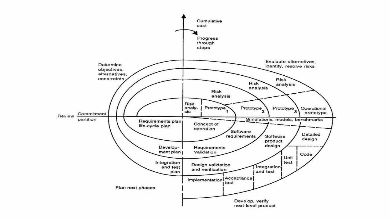


1

The Spiral Model
• A typical cycle of the spiral. Each cycle of the spiral begins with the identification of– the objectives of the portion of the product being elaborated
(performance, functionality, ability to accommodate change, etc.);– the alternative means of implementing this portion of the product
(design A , design B, reuse, buy, etc.); and– the constraints imposed on the application of the alternatives (cost,
schedule, inter-face, etc.).


2

The Spiral Model
• The next step is to evaluate the alternatives relative to the objectives and constraints.
• Frequently, this process will identify areas of uncertainty that are significant sources of project risk.
• If so, the next step should involve the formulation of a cost-effective strategy for resolving the sources of risk.
• This may involve prototyping, simulation, benchmarking, reference checking, administering user questionnaires, analytic modelling, or combinations of these and other risk resolution techniques.


3

The Spiral Model
• Once the risks are evaluated, the next step is determined by the relative remaining risks.
• If performance or user-interface risks strongly dominate program development or internal interface-control risks, the next step may be an evolutionary development one: a minimal effort to specify the overall nature of the product, a plan for the next level of prototyping, and the development of a more detailed prototype to continue to resolve the major risk issues.


4

The Spiral Model
• If this prototype is operationally useful and robust enough to serve as a low-risk base for future product evolution, the subsequent risk-driven steps would be the evolving series of evolutionary prototypes going toward the right of the figure.
• In this case, the option of writing specifications would be addressed but not exercised. Thus, risk considerations can lead to a project implementing only a subset of all the potential steps in the model.
• On the other hand, if previous prototyping efforts have already resolved all of the performance or user-interface risks, and program development or interface-control risks dominate, the next step follows the basic waterfall approach (concept of operation, soft-ware requirements, preliminary design, etc.), modified as appropriate to incorporate incremental development.
• Each level of software specification in the figure is then followed by a validation step and the preparation of plans for the succeeding cycle.

A prioritized top-ten list of software risk items

Risk Item Risk Management Techniques
1. Personnel shortfalls Staffing with top talent, job matching; teambuilding; morale building; cross-training; pre-scheduling key people
2. Unrealistic schedules and budgets Detailed, multisource cost and schedule estimation; design to cost; incremental development; software reuse; requirements scrubbing
3. Developing the wrong software functions
Organization analysis; mission analysis; ops-concept formulation; user surveys; prototyping; early users’ manuals
4. Developing the wrong user interface Task analysis; prototyping; scenarios; user characterization (functionality, style, workload)
5. Gold plating Requirements scrubbing; prototyping; cost-benefit analysis; design to cost
6. Continuing stream of requirement changes
High change threshold; information hiding; incremental development (defer changes to later increments)
7. Shortfalls in externally furnished components
Benchmarking; inspections; reference checking; compatibility analysis
8. Shortfalls in externally performed tasks Reference checking; pre-award audits; award-fee contracts; competitive design or prototyping; teambuilding
9. Real-time performance shortfalls Simulation; benchmarking; modelling; prototyping; instrumentation; tuning
10. Straining computer-science capabilities Technical analysis; cost—benefit analysis; prototyping; reference checking

1990s: The V-Model andRapid Application Development

The Relationship of System Engineering to the Project Cycle by
Kevin Forsberg and Harold Mooz
Reference
• Forsberg, K., Mooz, H., 1991, "The Relationship of System Engineering to the Project Cycle", Chattanooga, Tennessee: Proceedings of the National Council for Systems Engineering (NCOSE) Conference, pp. 57–65.

Abstract• “A new way of portraying the technical aspect of the project cycle
clarifies the role and responsibility of system engineering to a project. This new three dimensional graphic illustrates the end-to-end involvement of system engineering in the project cycle, clarifies the relationship of system engineering and design engineering, and encourages the implementation of concurrent engineering.”

Introduction
• The Waterfall Model has a deficiency in that it implies that the work downstream cannot begin until the upstream major reviews have occurred.

Introduction
• The Spiral Model is better since it ensures prototyping occurs earlier, but the role of software engineering in the overall process is unclear.

The “Vee” Model
• Start with the user needs on the upper right, and ending with a user-validated system on the upper right.
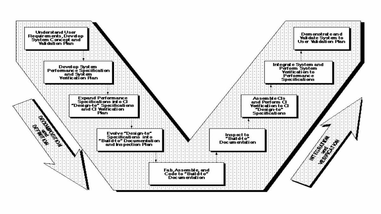

Detailed Discussion of the “Vee” Model
• Start with the user needs on the upper right, and ending with a user-validated system on the upper right.

Detailed Discussion of the “Vee” Model
• As project development progresses, a series of six baselines are established to systematically manage cohesive system development:– The first is the “User Requirements Baseline” established by the System Requirement Document
approved and put under Configuration Management prior to the System Requirements Review. – The second is the “Concept Baseline” established by the Concept Definition section of the Integrated
Program Summary document at the System Requirements Review. – The third is the “System Performance Baseline” (or Development Baseline) established by the System
Performance Specification at the System Design Review.– The fourth is the “‘Design-To’ Baseline” (or Allocated Baseline) established at the series of Preliminary
Design Reviews. – The fifth is the “‘Build-To’ Baseline” (or preliminary Product Baseline) established at the series of Critical
Design Reviews. – The sixth is the “‘As-Built’ Baseline” (or Production Baseline) established at the series of Formal
Qualification Reviews (FQRs). Each of the baselines is put under formal Configuration Management at the time they are approved.

Detailed Discussion of the “Vee” Model
• Incremental Development • If the User Requirements are too vague to permit final
definition at Preliminary Design Review, one approach is to develop the project in predetermined incremental releases.
• The first release is focused on meeting a minimum set of User Requirements, with subsequent releases providing added functionality and performance. This is a common approach in software development.

Detailed Discussion of the “Vee” Model
• Concurrent Engineering• If high iteration with User Requirements is required after the
System Design Review (SDR), it is probable that the project has passed early Control Gates prematurely, and it is not sufficiently defined.
• One cause of premature advance is that the appropriate technical experts were not involved at early stages, resulting in acceptance of requirements and design concepts which cannot be built, inspected, and/or maintained.


RAD: Rapid Application Development by
James Martin

Reference
• Martin, J., RAD: Rapid Application Development, 1991, MacMillan Publishing Co., New York.

James Martin
• Born in 1933.• Born in Ashby, Leicestershire• a British Information Technology
consultant and author, who was nominated for a Pulitzer prize for his book, The Wired Society: A Challenge for Tomorrow (1977).

Rapid Application Development
• Rapid Application Development– 1. Joint Requirements Planning (JRP)– 2. Joint Application Design (JAD)– 3. Construction
• Heavy use of tools: code generators• Time-boxed; many prototypes
– 4. Cutover• Good for systems with extensive user input available

Rapid Application Development

Rapid Application Development

Rapid Application Development• RAD is a way to deliver systems very fast
– The longer a project, the greater its likelihood of failure• It is a lightweight approach• Uses proven technology effectively• Make the solution fit within the capabilities of the tools (hammer?)• RAD is not Quick and Dirty with a thin veneer of discipline• RAD operates where the 80 / 20 rule applies• RAD can’t be used in all situations

2000s: Agile Development

Manifesto for Agile Software Developmentby
Kent BeckMike Beedle
Arie van BennekumAlistair Cockburn
Ward CunninghamMartin Fowler
James GrenningJim HighsmithAndrew HuntRon Jeffries
Jon KernBrian Marick
Robert C. MartinSteve Mellor
Ken SchwaberJeff SutherlandDave Thomas

Reference
• Beck, K. et al., 2001, "Manifesto for Agile Software Development“, Agile Alliance.

Background
• In February 2001, 17 software developers met at the Snowbird, Utah resort, to discuss lightweight development methods.
• They published the Manifesto for Agile Software Development to define the approach now known as agile software development.
• Some of the manifesto's authors formed the Agile Alliance, a non-profit organization that promotes software development according to the manifesto's principles.

Manifesto for Agile Software Development
We are uncovering better ways of developingsoftware by doing it and helping others do it.
Through this work we have come to value:
Individuals and interactions over processes and toolsWorking software over comprehensive documentation
Customer collaboration over contract negotiationResponding to change over following a plan
That is, while there is value in the items onthe right, we value the items on the left more.

Agile Methods
• Well-known agile software development methods include:– Agile Modelling– Agile Unified Process (AUP)– Dynamic Systems Development Method (DSDM)– Essential Unified Process (EssUP)– Extreme Programming (XP)– Feature Driven Development (FDD)– Open Unified Process (OpenUP)– Scrum– Velocity tracking

Computer Networks
Damian Gordon

• When we hook up computers together using data communication facilities, we call this a computer network.
Computer Networks
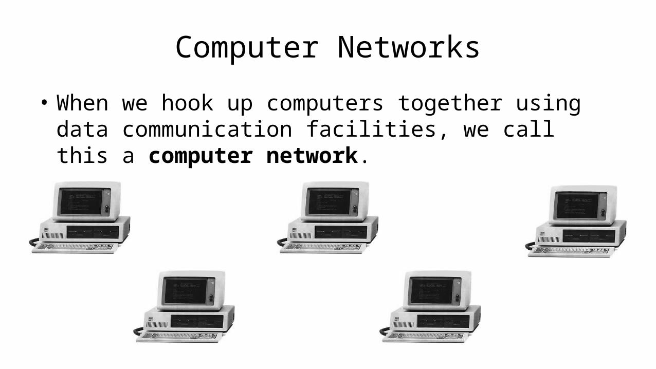
• When we hook up computers together using data communication facilities, we call this a computer network.
Computer Networks

• When we hook up computers together using data communication facilities, we call this a computer network.
Computer Networks

• When we hook up computers together using data communication facilities, we call this a computer network.
Computer Networks
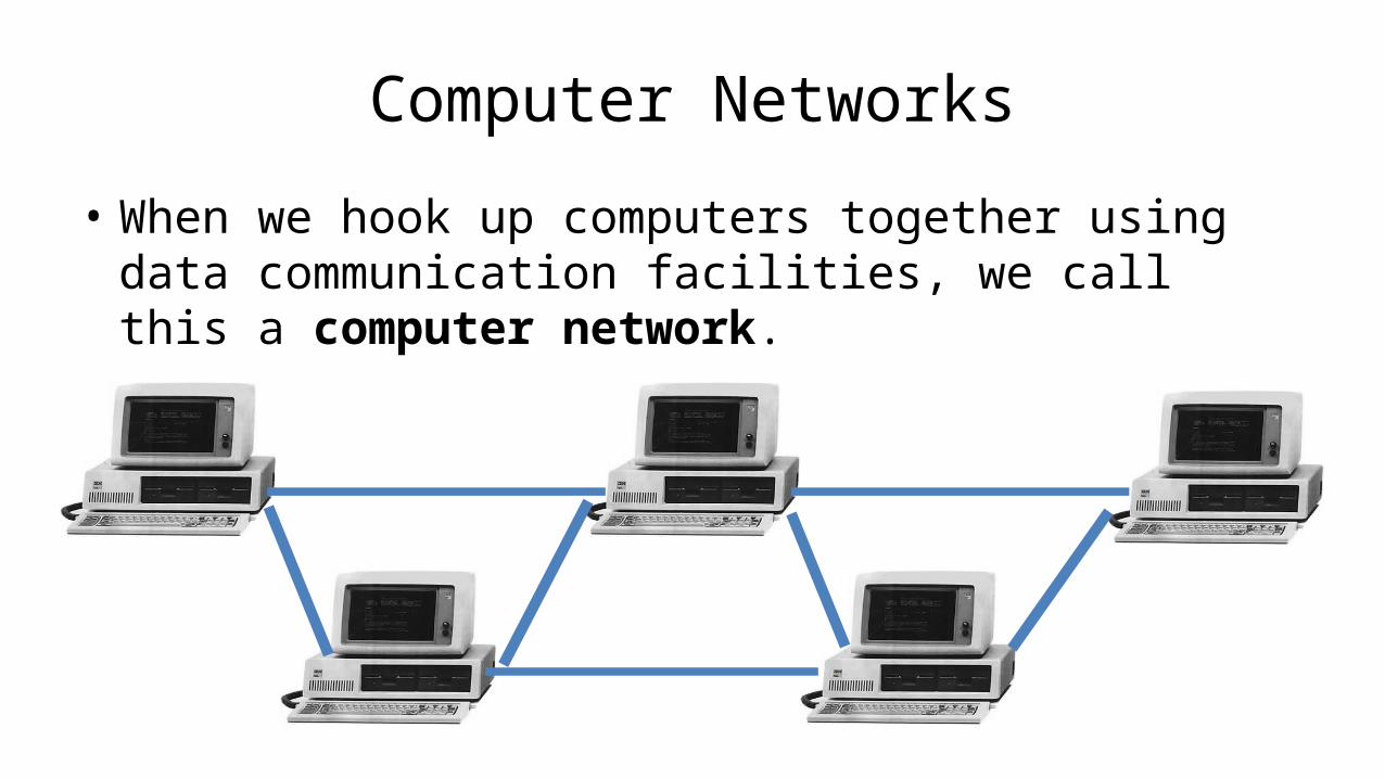
• When we hook up computers together using data communication facilities, we call this a computer network.
Computer Networks

• We can classify networks by the geographical distance they cover:
– Local Area Network (LAN)– Metropolitan Area Network (MAN)– Wide Area Network (WAN)
– Wireless Local Area Network (WLAN)
Network Types

Network Types
WANLAN MAN

• A Local Area Network (LAN) is a network within a single building or campus, e.g. an office, a college, or a warehouse. It is typically owned and used by a single organisation. Typically it’s a cluster of PCs or workstations. A LAN can be linked to larger networks via a bridge or gateway.
Network Types

• A Metropolitan Area Network (MAN) is a network that covers a full street, a neighbourhood, or even a city, as long as it doesn’t exceed a circumference of 100 kilometres. The MAN is often owned and run as a public utility, and are typically configured as a Ring Topology.
Network Types

• A Wide Area Network (WAN) is a network that a country, or connects countries. The WAN is often owned and run as a public utility, but telephone companies have WANs also. WANs can use anything for satellites to microwaves transmissions. The most common example of a WAN is the Internet, but there are other commercial WANs.
Network Types

• A Wireless Local Area Network (WLAN) is a wireless LAN. It works exactly the same as a normal LAN, but the technology means that the network uses a wireless protocol such as IEEE 802.11a, IEEE 802.11b, IEEE 802.11g, or IEEE 802.11n. Additionally 802.16 (the mobile WiMAX standard) is available.
Network Types