5.3 dynamic programming

Chapter 8Chapter 8

Dynamic ProgrammingDynamic Programming

Copyright © 2007 Pearson Addison-Wesley. All rights reserved.

8-2Copyright © 2007 Pearson Addison-Wesley. All rights reserved. A. Levitin “Introduction to the Design & Analysis of Algorithms,” 2nd ed., Ch. 8

Dynamic ProgrammingDynamic Programming

DDynamic Programming ynamic Programming is a general algorithm design technique is a general algorithm design technique for solving problems defined by or formulated as recurrences for solving problems defined by or formulated as recurrences with overlapping subinstanceswith overlapping subinstances

• Invented by American mathematician Richard Bellman in the Invented by American mathematician Richard Bellman in the 1950s to solve optimization problems and later assimilated by CS1950s to solve optimization problems and later assimilated by CS

• “ “Programming” here means “planning”Programming” here means “planning”

• Main idea:Main idea:- set up a recurrence relating a solution to a larger instance set up a recurrence relating a solution to a larger instance

to solutions of some smaller instancesto solutions of some smaller instances- solve smaller instances once- solve smaller instances once- record solutions in a table record solutions in a table - extract solution to the initial instance from that tableextract solution to the initial instance from that table


Example: Fibonacci numbersExample: Fibonacci numbers

• Recall definition of Fibonacci numbers:Recall definition of Fibonacci numbers:

FF((nn)) = F = F((nn-1)-1) + F + F((nn-2)-2)FF(0)(0) = = 00FF(1)(1) = = 11

• Computing the Computing the nnthth Fibonacci number recursively (top-down): Fibonacci number recursively (top-down):

FF((nn))

FF((n-n-1) 1) + F + F((n-n-2)2)

FF((n-n-2) 2) + F+ F((n-n-3) 3) FF((n-n-3) 3) + F+ F((n-n-4)4)

......


Example: Fibonacci numbers (cont.)Example: Fibonacci numbers (cont.)

Computing the Computing the nnthth Fibonacci number using bottom-up iteration and Fibonacci number using bottom-up iteration and recording results:recording results:

FF(0)(0) = = 00 FF(1)(1) = = 11 FF(2)(2) = = 1+0 = 11+0 = 1 … … FF((nn-2) = -2) = FF((nn-1) = -1) = FF((nn) = ) = FF((nn-1)-1) + F + F((nn-2)-2)

Efficiency:Efficiency: - time- time - space- space

0

1

1

. . .

F(n-2)

F(n-1)

F(n)

n n

What if we solve it recursively?


Examples of DP algorithmsExamples of DP algorithms

• Computing a binomial coefficientComputing a binomial coefficient

• Longest common subsequenceLongest common subsequence

• Warshall’s algorithm for transitive closureWarshall’s algorithm for transitive closure

• Floyd’s algorithm for all-pairs shortest pathsFloyd’s algorithm for all-pairs shortest paths

• Constructing an optimal binary search treeConstructing an optimal binary search tree

• Some instances of difficult discrete optimization problems:Some instances of difficult discrete optimization problems: - traveling salesman- traveling salesman - knapsack- knapsack


Computing a binomial coefficient by DPComputing a binomial coefficient by DP

Binomial coefficients are coefficients of the binomial formula:Binomial coefficients are coefficients of the binomial formula:((a + ba + b))nn = = CC((nn,0),0)aannbb0 0 + . . . + + . . . + CC((nn,,kk))aan-kn-kbbkk + . . . + . . . + CC((nn,,nn))aa00bbnn

Recurrence: Recurrence: CC((nn,,kk) = ) = CC((n-n-1,1,kk) + ) + CC((nn-1,-1,kk-1) for -1) for n > k n > k > 0> 0 CC((nn,0) = 1, ,0) = 1, CC((nn,,nn) = 1 for ) = 1 for n n 0 0 Value of Value of CC((nn,,kk) can be computed by filling a table:) can be computed by filling a table:

0 1 2 . . . 0 1 2 . . . kk-1 -1 kk 0 10 1 1 1 11 1 1 .. .. .. n-n-1 1 CC((n-n-1,1,kk-1) -1) CC((n-n-1,1,kk) ) nn C C((nn,,kk) )


Computing Computing CC((n,kn,k): pseudocode and analysis): pseudocode and analysis

Time efficiency: Time efficiency: ΘΘ((nknk))

Space efficiency: Space efficiency: ΘΘ((nknk))


Knapsack Problem by DPKnapsack Problem by DP

Given Given nn items of items of

integer weights: integer weights: ww1 1 ww22 … w … wnn

values: values: vv1 1 vv22 … v … vnn

a knapsack of integer capacity a knapsack of integer capacity WW find most valuable subset of the items that fit into the knapsackfind most valuable subset of the items that fit into the knapsack

Consider instance defined by first Consider instance defined by first i i items and capacity items and capacity j j ((j j WW))..

Let Let VV[[ii,,jj] be optimal value of such an instance. Then] be optimal value of such an instance. Then

max {max {VV[[ii-1,-1,jj], ], vvii + + VV[[ii-1,-1,j- j- wwii]} if ]} if j- j- wwi i 0 0VV[[ii,,jj] =] =

VV[[ii-1,-1,jj] if ] if j- j- wwi i < 0< 0

Initial conditions: Initial conditions: VV[0,[0,jj] = 0 and ] = 0 and VV[[ii,0] = 0,0] = 0

{


Knapsack Problem by DP (example)Knapsack Problem by DP (example)

Example: Knapsack of capacity Example: Knapsack of capacity W W = 5= 5item weight value item weight value 1 2 $121 2 $12 2 1 $102 1 $10 3 3 $203 3 $20 4 2 $15 capacity 4 2 $15 capacity jj

0 1 2 3 40 1 2 3 4 55 00

ww1 1 = 2, = 2, vv11== 12 112 1

ww2 2 = 1, = 1, vv22== 10 210 2

ww3 3 = 3, = 3, vv33== 20 320 3

ww4 4 = 2, = 2, vv44== 15 415 4 ??

0 0 0

0 0 12

0 10 12 22 22 22

0 10 12 22 30 32

0 10 15 25 30 37

Backtracing finds the actual optimal subset, i.e. solution.


Knapsack Problem by DP (pseudocode)Knapsack Problem by DP (pseudocode)

Algorithm DPKnapsack(Algorithm DPKnapsack(ww[[11....nn], ], vv[[1..n1..n], ], WW))var var VV[[0..n,0..W0..n,0..W]], P, P[[1..n,1..W1..n,1..W]]:: int intfor for j := 0j := 0 to to WW do do

VV[[0,j0,j] := ] := 00 for for i := 0i := 0 to to nn do do VV[[i,0i,0]] := 0 := 0 for for i := 1i := 1 to to nn do do

for for j := 1j := 1 to to WW do doif if ww[[ii] ] j j and and vv[[ii]] + V + V[[i-1,j-wi-1,j-w[[ii]]]] > V > V[[i-1,ji-1,j] then] then

VV[[i,ji,j] ] := v:= v[[ii]] + V + V[[i-1,j-wi-1,j-w[[ii]]]]; P; P[[i,ji,j]] := j-w := j-w[[ii]]else else

VV[[i,ji,j]] := V := V[[i-1,ji-1,j]]; P; P[[i,ji,j]] := j := jreturn return VV[[n,Wn,W] and the optimal subset by backtracing] and the optimal subset by backtracing

Running time and space: O(nW).


Longest Common Subsequence (LCS)Longest Common Subsequence (LCS)

A subsequence of a sequence/string A subsequence of a sequence/string S S is obtained by is obtained by deleting zero or more symbols from deleting zero or more symbols from SS. For example, the . For example, the following are following are somesome subsequences of “president”: pred, sdn, subsequences of “president”: pred, sdn, predent. In other words, the letters of a subsequence of S predent. In other words, the letters of a subsequence of S appear in order inappear in order in S S, but they are not required to be , but they are not required to be consecutive.consecutive.

The longest common subsequence problem is to find a The longest common subsequence problem is to find a maximum length common subsequence between two maximum length common subsequence between two sequences.sequences.


LCSLCS

For instance,For instance,

Sequence 1: presidentSequence 1: president

Sequence 2: providenceSequence 2: providence

Its LCS is priden.Its LCS is priden.

president

providence


LCSLCS

Another example:Another example:

Sequence 1: algorithmSequence 1: algorithm

Sequence 2: alignmentSequence 2: alignment

One of its LCS is algm.One of its LCS is algm.

a l g o r i t h m

a l i g n m e n t


How to compute LCS?How to compute LCS?

Let ALet A=a=a11aa22…a…am m and and B=bB=b11bb22…b…bnn . .

lenlen((i, ji, j): the length of an LCS between ): the length of an LCS between aa11aa22…a…ai i and and bb11bb22…b…bjj

With proper initializations, With proper initializations, lenlen((i, ji, j) can be computed as follows.) can be computed as follows.

,

. and 0, if)),1(),1,(max(

and 0, if1)1,1(

,0or 0 if0

),(

ji

ji

bajijilenjilen

bajijilen

ji

jilen


p r o c e d u r e L C S - L e n g t h ( A , B )

1 . f o r i ← 0 t o m d o l e n ( i , 0 ) = 0

2 . f o r j ← 1 t o n d o l e n ( 0 , j ) = 0

3 . f o r i ← 1 t o m d o

4 . f o r j ← 1 t o n d o

5 . i f ji ba t h e n

" "),(

1)1,1(),(

jiprev

jilenjilen

6 . e l s e i f )1,(),1( jilenjilen

7 . t h e n

" "),(

),1(),(

jiprev

jilenjilen

8 . e l s e

" "),(

)1,(),(

jiprev

jilenjilen

9 . r e t u r n l e n a n d p r e v


i j 0 1 p

2 r

3 o

4 v

5 i

6 d

7 e

8 n

9 c

10 e

0 0 0 0 0 0 0 0 0 0 0 0

1 p 2

0 1 1 1 1 1 1 1 1 1 1

2 r 0 1 2 2 2 2 2 2 2 2 2

3 e 0 1 2 2 2 2 2 3 3 3 3

4 s 0 1 2 2 2 2 2 3 3 3 3

5 i 0 1 2 2 2 3 3 3 3 3 3

6 d 0 1 2 2 2 3 4 4 4 4 4

7 e 0 1 2 2 2 3 4 5 5 5 5

8 n 0 1 2 2 2 3 4 5 6 6 6

9 t 0 1 2 2 2 3 4 5 6 6 6

Running time and memory: O(mn) and O(mn).


p r o c e d u r e O u tp u t - L C S ( A , p r e v , i , j )

1 i f i = 0 o r j = 0 t h e n r e t u r n

2 i f p r e v ( i , j ) = ” “ t h e n

ia

jiprevALCSOutput

print

)1,1,,(

3 e l s e i f p r e v ( i , j ) = ” “ t h e n O u tp u t - L C S ( A , p r e v , i - 1 , j )

4 e l s e O u tp u t - L C S ( A , p r e v , i , j - 1 )

The backtracing algorithm


i j 0 1 p

2 r

3 o

4 v

5 i

6 d

7 e

8 n

9 c

10 e

0 0 0 0 0 0 0 0 0 0 0 0

1 p 2

0 1 1 1 1 1 1 1 1 1 1

2 r 0 1 2 2 2 2 2 2 2 2 2

3 e 0 1 2 2 2 2 2 3 3 3 3

4 s 0 1 2 2 2 2 2 3 3 3 3

5 i 0 1 2 2 2 3 3 3 3 3 3

6 d 0 1 2 2 2 3 4 4 4 4 4

7 e 0 1 2 2 2 3 4 5 5 5 5

8 n 0 1 2 2 2 3 4 5 6 6 6

9 t 0 1 2 2 2 3 4 5 6 6 6

Output: priden


Warshall’s Algorithm: Transitive ClosureWarshall’s Algorithm: Transitive Closure

• Computes the transitive closure of a relationComputes the transitive closure of a relation

• Alternatively: existence of all nontrivial paths in a digraphAlternatively: existence of all nontrivial paths in a digraph

• Example of transitive closure:Example of transitive closure:

3

42

1

0 0 1 01 0 0 10 0 0 00 1 0 0

0 0 1 01 1 11 1 10 0 0 011 1 1 11 1

3

42

1


Warshall’s AlgorithmWarshall’s Algorithm

Constructs transitive closure Constructs transitive closure TT as the last matrix in the sequence as the last matrix in the sequence of of nn-by--by-n n matrices matrices RR(0)(0), … ,, … , RR((kk)), … ,, … , RR((nn)) wherewhereRR((kk))[[ii,,jj] = 1 iff there is nontrivial path from ] = 1 iff there is nontrivial path from ii to to jj with only the with only the first first k k vertices allowed as intermediate vertices allowed as intermediate Note that Note that RR(0) (0) = = A A (adjacency matrix)(adjacency matrix),, RR((nn))

= T = T (transitive closure)(transitive closure)

3

42

13

42

13

42

13

42

1

R(0)

0 0 1 01 0 0 10 0 0 00 1 0 0

R(1)

0 0 1 01 0 11 10 0 0 00 1 0 0

R(2)

0 0 1 01 0 1 10 0 0 01 1 1 1 11 1

R(3)

0 0 1 01 0 1 10 0 0 01 1 1 1

R(4)

0 0 1 01 11 1 10 0 0 01 1 1 1

3

42

1


Warshall’s Algorithm (recurrence)Warshall’s Algorithm (recurrence)

On theOn the k- k-th iteration, the algorithm determines for every pair of th iteration, the algorithm determines for every pair of vertices vertices i, ji, j if a path exists from if a path exists from i i andand j j with just vertices 1,…,with just vertices 1,…,k k allowedallowed asas intermediateintermediate

RR((kk-1)-1)[[i,ji,j]] (path using just 1 ,…, (path using just 1 ,…,k-k-1)1) RR((kk))[[i,ji,j] =] = oror

RR((kk-1)-1)[[i,ki,k] and ] and RR((kk-1)-1)[[k,jk,j]] (path from (path from i i to to kk and from and from kk to to jj using just 1 ,…,using just 1 ,…,k-k-1)1)

i

j

k

{

Initial condition?


Warshall’s Algorithm (matrix generation)Warshall’s Algorithm (matrix generation)

Recurrence relating elements Recurrence relating elements RR((kk)) to elements of to elements of RR((kk-1)-1) is: is:

RR((kk))[[i,ji,j] = ] = RR((kk-1)-1)[[i,ji,j] or] or ((RR((kk-1)-1)[[i,ki,k] and ] and RR((kk-1)-1)[[k,jk,j])])

It implies the following rules for generating It implies the following rules for generating RR((kk)) from from RR((kk-1)-1)::

Rule 1Rule 1 If an element in row If an element in row i i and column and column jj is 1 in is 1 in RR((k-k-1)1), , it remains 1 in it remains 1 in RR((kk))

Rule 2 Rule 2 If an element in row If an element in row i i and column and column jj is 0 in is 0 in RR((k-k-1)1),, it has to be changed to 1 in it has to be changed to 1 in RR((kk)) if and only if if and only if the element in its row the element in its row ii and column and column kk and the element and the element in its column in its column jj and row and row kk are both 1’s in are both 1’s in RR((k-k-1)1)


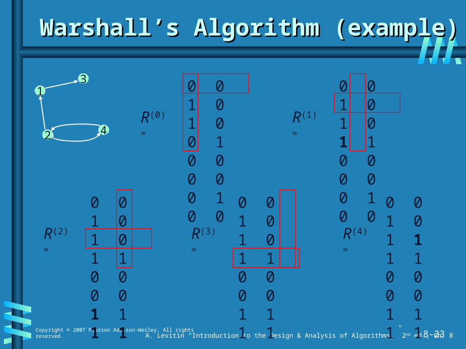
Warshall’s Algorithm (example)Warshall’s Algorithm (example)

3

42

1 0 0 1 01 0 0 10 0 0 00 1 0 0

R(0) =

0 0 1 01 0 1 10 0 0 00 1 0 0

R(1) =

0 0 1 01 0 1 10 0 0 01 1 1 1

R(2) =

0 0 1 01 0 1 10 0 0 01 1 1 1

R(3) =

0 0 1 01 1 1 10 0 0 01 1 1 1

R(4) =


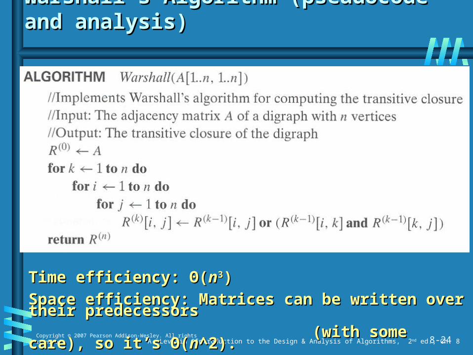
Warshall’s Algorithm (pseudocode and analysis)Warshall’s Algorithm (pseudocode and analysis)

Time efficiency: Time efficiency: ΘΘ((nn33))

Space efficiency: Matrices can be written over their predecessorsSpace efficiency: Matrices can be written over their predecessors

(with some care), so it’s (with some care), so it’s ΘΘ((nn^2).^2).


Floyd’s Algorithm: All pairs shortest pathsFloyd’s Algorithm: All pairs shortest paths

Problem: In a weighted (di)graph, find shortest paths betweenProblem: In a weighted (di)graph, find shortest paths between every pair of vertices every pair of vertices

Same idea: construct solution through series of matrices Same idea: construct solution through series of matrices DD(0)(0), …,, …, D D ((nn)) using increasing subsets of the vertices allowed using increasing subsets of the vertices allowed as intermediate as intermediate

Example:Example: 3

42

14

16

1

5

3

0 ∞ 4 ∞ 1 0 4 3 ∞ ∞ 0 ∞6 5 1 0


Floyd’s Algorithm (matrix generation)Floyd’s Algorithm (matrix generation)

On theOn the k- k-th iteration, the algorithm determines shortest paths th iteration, the algorithm determines shortest paths between every pair of vertices between every pair of vertices i, j i, j that use only vertices among 1,that use only vertices among 1,…,…,k k as intermediateas intermediate

DD((kk))[[i,ji,j] = min {] = min {DD((kk-1)-1)[[i,ji,j], ], DD((kk-1)-1)[[i,ki,k] + ] + DD((kk-1)-1)[[k,jk,j]}]}

i

j

k

DD((kk-1)-1)[[i,ji,j]]

DD((kk-1)-1)[[i,ki,k]]

DD((kk-1)-1)[[k,jk,j]]

Initial condition?


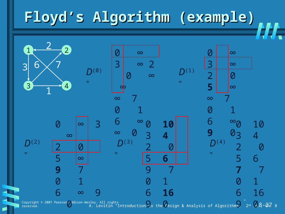
Floyd’s Algorithm (example)Floyd’s Algorithm (example)

0 ∞ 3 ∞ 2 0 ∞ ∞∞ 7 0 16 ∞ ∞ 0

D(0) =

0 ∞ 3 ∞ 2 0 5 ∞∞ 7 0 16 ∞ 9 0

D(1) =

0 ∞ 3 ∞2 0 5 ∞9 7 0 16 ∞ 9 0

D(2) =

0 10 3 42 0 5 69 7 0 16 16 9 0

D(3) =

0 10 3 42 0 5 67 7 0 16 16 9 0

D(4) =

31

3

2

6 7

4

1 2


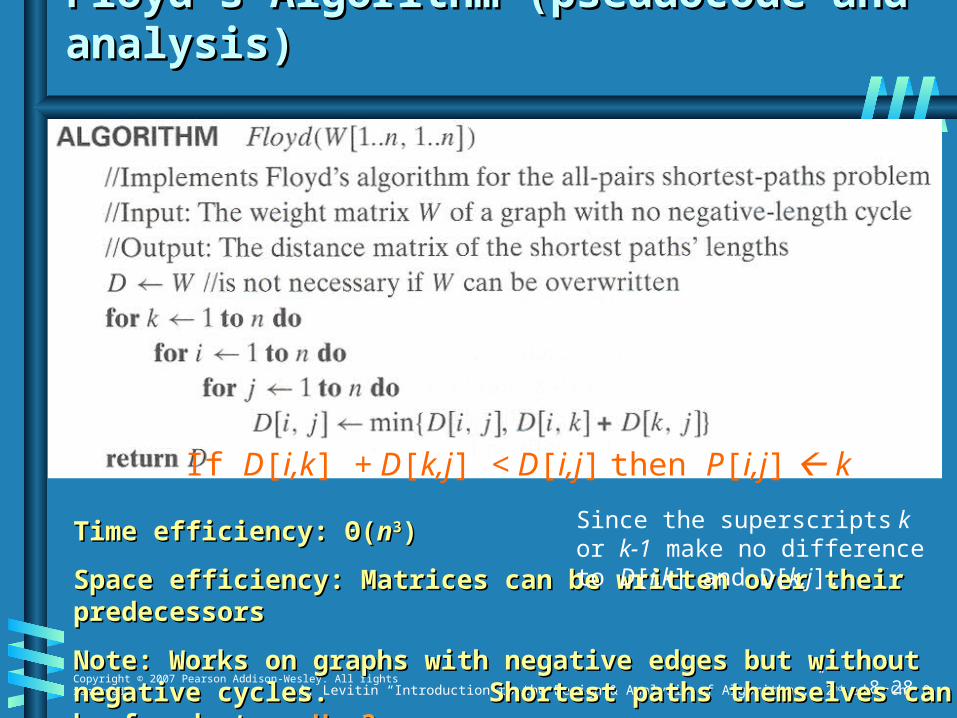
Floyd’s Algorithm (pseudocode and analysis)Floyd’s Algorithm (pseudocode and analysis)

Time efficiency: Time efficiency: ΘΘ((nn33))

Space efficiency: Matrices can be written over their predecessorsSpace efficiency: Matrices can be written over their predecessors

Note: Works on graphs with negative edges but without negative cycles. Note: Works on graphs with negative edges but without negative cycles. Shortest paths themselves can be found, too. Shortest paths themselves can be found, too. How?How?

If D[i,k] + D[k,j] < D[i,j] then P[i,j] k

Since the superscripts k or k-1 make no difference to D[i,k] and D[k,j].


Optimal Binary Search TreesOptimal Binary Search Trees

Problem: Given Problem: Given n n keys keys aa1 1 < …< < …< aan n and probabilities and probabilities pp11,, …, …, ppnn

searching for them, find a BST with a minimumsearching for them, find a BST with a minimum

average number of comparisons in successful search. average number of comparisons in successful search.

Since total number of BSTs with Since total number of BSTs with n n nodes is given by nodes is given by C(2C(2nn,,nn)/()/(nn+1), which grows exponentially, brute force is hopeless. +1), which grows exponentially, brute force is hopeless.

Example: What is an optimal BST for keys Example: What is an optimal BST for keys AA, , BB,, C C, and , and D D withwith search probabilities 0.1, 0.2, 0.4, and 0.3, respectively? search probabilities 0.1, 0.2, 0.4, and 0.3, respectively?

D

A

B

C

Average # of comparisons = 1*0.4 + 2*(0.2+0.3) + 3*0.1 = 1.7


DP for Optimal BST ProblemDP for Optimal BST Problem

Let Let CC[[i,ji,j] be minimum average number of comparisons made in ] be minimum average number of comparisons made in T[T[i,ji,j], optimal BST for keys ], optimal BST for keys aaii < …< < …< aajj ,, where 1 ≤ where 1 ≤ i i ≤ ≤ j j ≤ ≤ n. n.

Consider optimal BST among all BSTs with some Consider optimal BST among all BSTs with some aak k ((i i ≤ ≤ k k ≤≤ jj ) )

as their root; T[as their root; T[i,ji,j] is the best among them. ] is the best among them.

a

OptimalBST for

a , ..., a

OptimalBST for

a , ..., ai

k

k-1 k+1 j

CC[[i,ji,j] =] =

min {min {ppk k · · 1 +1 +

∑ ∑ ppss (level (level aas s in T[in T[i,k-i,k-1] +1)1] +1) ++

∑ ∑ ppss (level (level aass in T[in T[k+k+11,j,j] +1)}] +1)}

i i ≤ ≤ k k ≤≤ jj

s s == ii

k-k-11

s =s =k+k+11

jj


goal0

0

C[i,j]

0

1

n+1

0 1 n

p 1

p2

np

i

j

DP for Optimal BST Problem (cont.)DP for Optimal BST Problem (cont.)

After simplifications, we obtain the recurrence for After simplifications, we obtain the recurrence for CC[[i,ji,j]:]:

CC[[i,ji,j] = ] = min {min {CC[[ii,,kk-1] + -1] + CC[[kk+1,+1,jj]} + ∑ ]} + ∑ ppss forfor 1 1 ≤≤ i i ≤≤ j j ≤≤ nn

CC[[i,ii,i] = ] = ppi i for 1 for 1 ≤≤ i i ≤≤ j j ≤≤ nn

s s == ii

jj

i i ≤≤ k k ≤≤ jj

Example: key Example: key A B C DA B C D

probability 0.1 0.2 0.4 0.3probability 0.1 0.2 0.4 0.3

The tables below are filled diagonal by diagonal: the left one is filled The tables below are filled diagonal by diagonal: the left one is filled using the recurrence using the recurrence CC[[i,ji,j] = ] = min {min {CC[[ii,,kk-1] + -1] + CC[[kk+1,+1,jj]} + ∑ ]} + ∑ pps , s , CC[[i,ii,i] = ] = ppi i ;;

the right one, for trees’ roots, records the right one, for trees’ roots, records kk’s values giving the minima’s values giving the minima

00 11 22 33 44

11 00 .1.1 .4.4 1.11.1 1.71.7

22 00 .2.2 .8.8 1.41.4

33 00 .4.4 1.01.0

44 00 .3.3

55 00

00 11 22 33 44

11 11 22 33 33

22 22 33 33

33 33 33

44 44

55

i i ≤ ≤ k k ≤≤ jj s s == ii

jj

optimal BSToptimal BST

B

A

C

D

i i jji i jj


Optimal Binary Search TreesOptimal Binary Search Trees


Analysis DP for Optimal BST ProblemAnalysis DP for Optimal BST Problem

Time efficiency: Time efficiency: ΘΘ((nn33) but can be reduced to ) but can be reduced to ΘΘ((nn22)) by takingby taking advantage of monotonicity of entries in the advantage of monotonicity of entries in the root table, i.e., root table, i.e., RR[[i,ji,j] is always in the range ] is always in the range between between RR[[i,ji,j-1] and R[-1] and R[ii+1,j]+1,j]

Space efficiency: Space efficiency: ΘΘ((nn22))

Method can be expanded to include unsuccessful searchesMethod can be expanded to include unsuccessful searches

Education

5.3 dynamic programming