Embed Size (px)
Citation preview

1
Decision Tree Induction
2
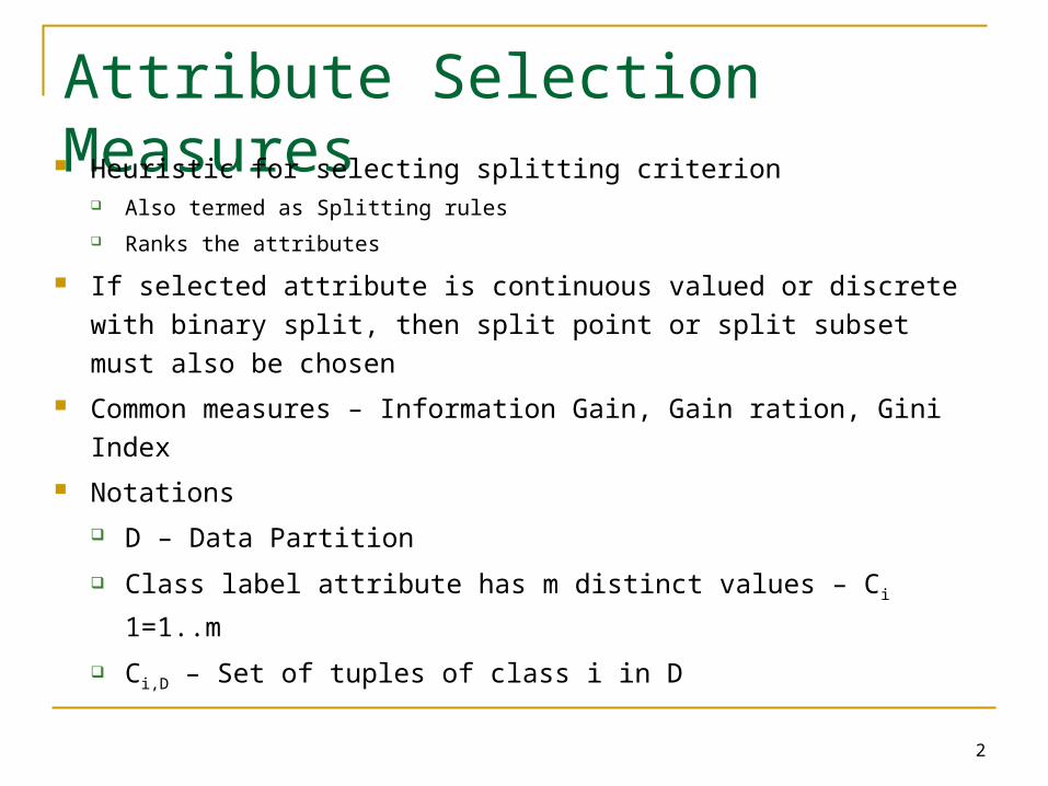
Attribute Selection Measures Heuristic for selecting splitting criterion
Also termed as Splitting rules
Ranks the attributes
If selected attribute is continuous valued or discrete with binary split,
then split point or split subset must also be chosen
Common measures – Information Gain, Gain ration, Gini Index
Notations
D – Data Partition
Class label attribute has m distinct values – Ci 1=1..m
Ci,D – Set of tuples of class i in D
3
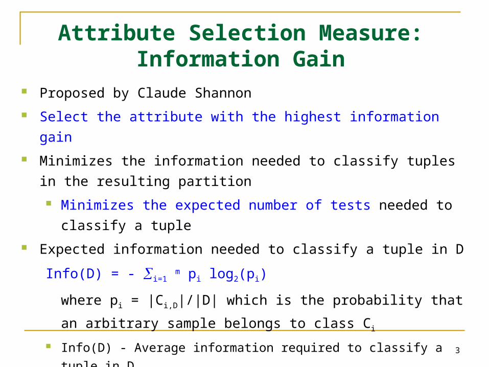
Attribute Selection Measure: Information Gain
Proposed by Claude Shannon
Select the attribute with the highest information gain
Minimizes the information needed to classify tuples in the
resulting partition
Minimizes the expected number of tests needed to classify
a tuple
Expected information needed to classify a tuple in D
Info(D) = - i=1 m pi log2(pi)
where pi = |Ci,D|/|D| which is the probability that an
arbitrary sample belongs to class Ci
Info(D) - Average information required to classify a tuple in D
Info(D) is also known as entropy of D
4
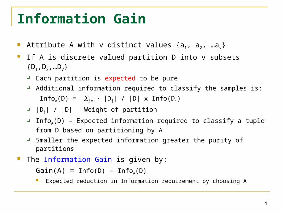
Information Gain
Attribute A with v distinct values {a1, a2, …av}
If A is discrete valued partition D into v subsets {D1,D2,…DV} Each partition is expected to be pure Additional information required to classify the samples is:
InfoA(D) = j=1 v |Dj| / |D| x Info(Dj)
|Dj| / |D| - Weight of partition
InfoA(D) – Expected information required to classify a tuple from D based
on partitioning by A Smaller the expected information greater the purity of partitions
The Information Gain is given by:
Gain(A) = Info(D) – InfoA(D) Expected reduction in Information requirement by choosing A
5
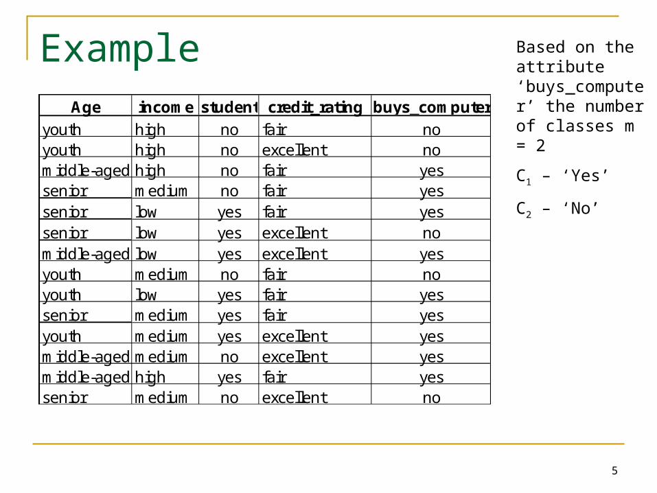
ExampleAge income student credit_rating buys_computer
youth high no fair noyouth high no excellent nomiddle-aged high no fair yessenior medium no fair yessenior low yes fair yessenior low yes excellent nomiddle-aged low yes excellent yesyouth medium no fair noyouth low yes fair yessenior medium yes fair yesyouth medium yes excellent yesmiddle-aged medium no excellent yesmiddle-aged high yes fair yessenior medium no excellent no
Based on the attribute ‘buys_computer’ the number of classes m = 2
C1 – ‘Yes’
C2 – ‘No’
6
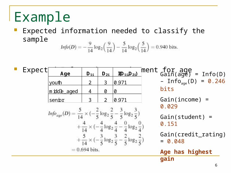
Example Expected information needed to classify the sample
Expected Information requirement for age
Age D1i D2i I(D1i,D2i)
youth 2 3 0.971
middle_aged 4 0 0
senior 3 2 0.971
Gain(age) = Info(D) – Infoage(D) = 0.246 bits
Gain(income) = 0.029
Gain(student) = 0.151
Gain(credit_rating) = 0.048
Age has highest gain
7
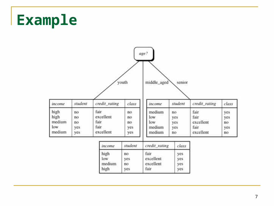
Example
8
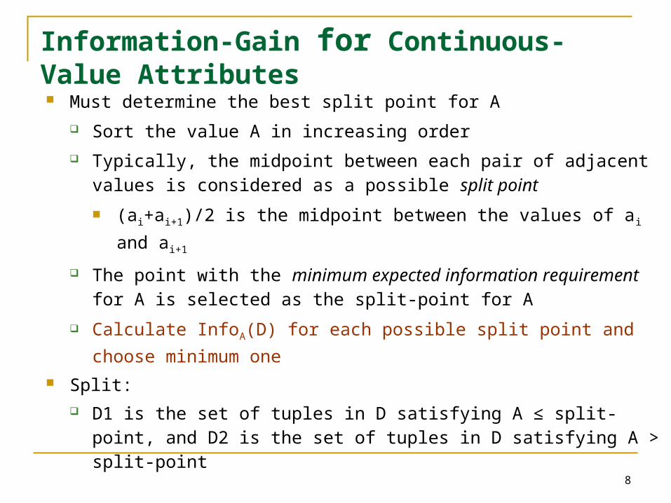
Information-Gain for Continuous-Value Attributes Must determine the best split point for A
Sort the value A in increasing order
Typically, the midpoint between each pair of adjacent values is considered as a possible split point
(ai+ai+1)/2 is the midpoint between the values of ai and ai+1
The point with the minimum expected information requirement for A is selected as the split-point for A
Calculate InfoA(D) for each possible split point and choose minimum
one Split:
D1 is the set of tuples in D satisfying A ≤ split-point, and D2 is the set of tuples in D satisfying A > split-point
9
Gain Ratio for Attribute Selection
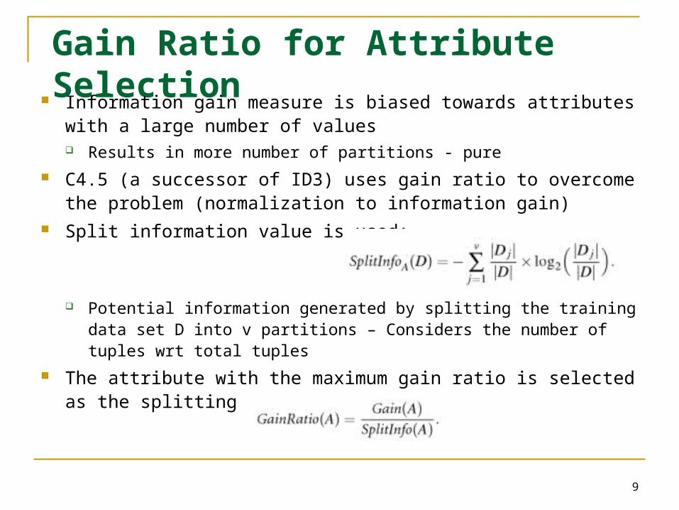
Information gain measure is biased towards attributes with a large number of values Results in more number of partitions - pure
C4.5 (a successor of ID3) uses gain ratio to overcome the problem (normalization to information gain)
Split information value is used:
Potential information generated by splitting the training data set D into v partitions – Considers the number of tuples wrt total tuples
The attribute with the maximum gain ratio is selected as the splitting attribute
10
Gain Ratio - Example
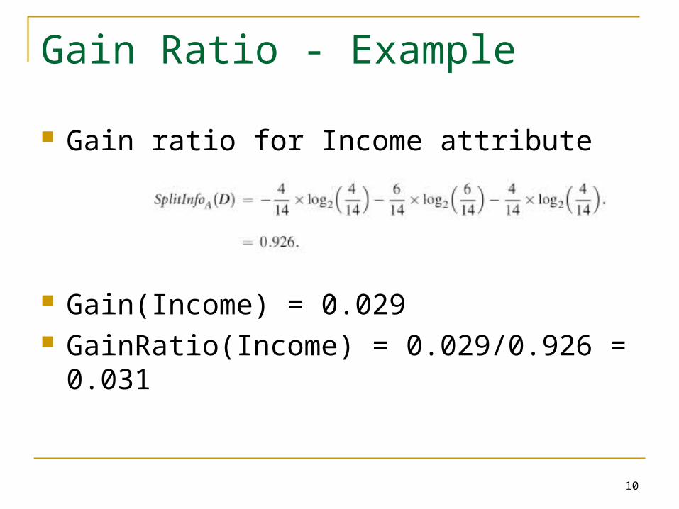
Gain ratio for Income attribute
Gain(Income) = 0.029 GainRatio(Income) = 0.029/0.926 = 0.031
11
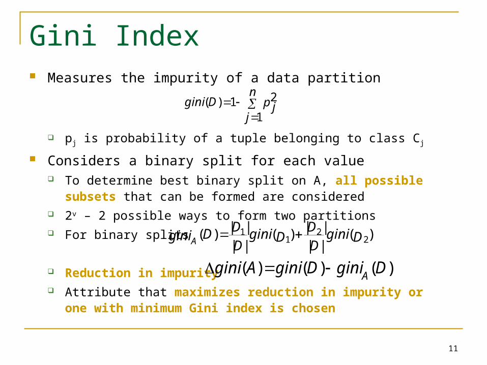
Gini Index Measures the impurity of a data partition
pj is probability of a tuple belonging to class Cj
Considers a binary split for each value To determine best binary split on A, all possible subsets that can be
formed are considered 2v – 2 possible ways to form two partitions For binary splits
Reduction in impurity Attribute that maximizes reduction in impurity or one with minimum
Gini index is chosen
n
jp jDgini
1
21)(
)(||||)(
||||)( 2
21
1 DginiDD
DginiDDDginiA
)()()( DginiDginiAginiA
12
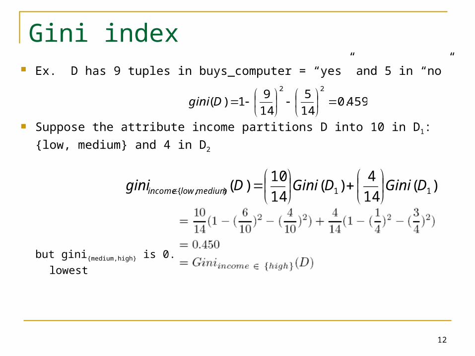
Gini index Ex. D has 9 tuples in buys_computer = “yes” and 5 in “no”
Suppose the attribute income partitions D into 10 in D1: {low, medium}
and 4 in D2
but gini{medium,high} is 0.30 and thus the best since it is the lowest
459.014
5
14
91)(
22
Dgini
)(14
4)(
14
10)( 11},{ DGiniDGiniDgini mediumlowincome
13
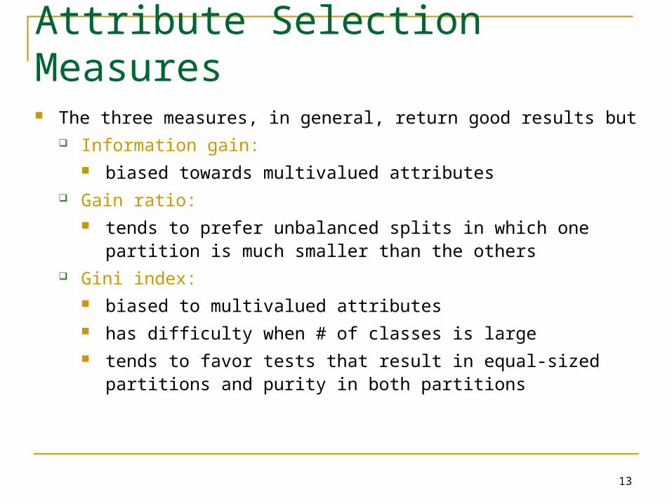
Attribute Selection Measures
The three measures, in general, return good results but Information gain:
biased towards multivalued attributes Gain ratio:
tends to prefer unbalanced splits in which one partition is much smaller than the others
Gini index: biased to multivalued attributes has difficulty when # of classes is large tends to favor tests that result in equal-sized partitions and
purity in both partitions
14
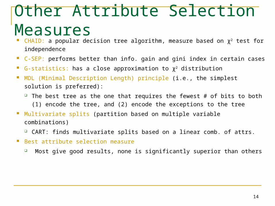
Other Attribute Selection Measures CHAID: a popular decision tree algorithm, measure based on χ2 test for
independence
C-SEP: performs better than info. gain and gini index in certain cases
G-statistics: has a close approximation to χ2 distribution
MDL (Minimal Description Length) principle (i.e., the simplest solution is
preferred):
The best tree as the one that requires the fewest # of bits to both (1)
encode the tree, and (2) encode the exceptions to the tree
Multivariate splits (partition based on multiple variable combinations)
CART: finds multivariate splits based on a linear comb. of attrs.
Best attribute selection measure
Most give good results, none is significantly superior than others
15
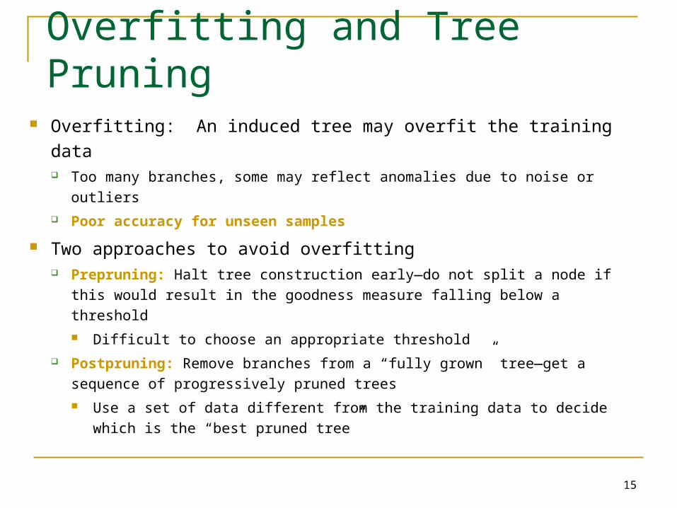
Overfitting and Tree Pruning
Overfitting: An induced tree may overfit the training data Too many branches, some may reflect anomalies due to noise or outliers
Poor accuracy for unseen samples
Two approaches to avoid overfitting Prepruning: Halt tree construction early—do not split a node if this would
result in the goodness measure falling below a threshold
Difficult to choose an appropriate threshold
Postpruning: Remove branches from a “fully grown” tree—get a sequence
of progressively pruned trees
Use a set of data different from the training data to decide which is the
“best pruned tree”
16
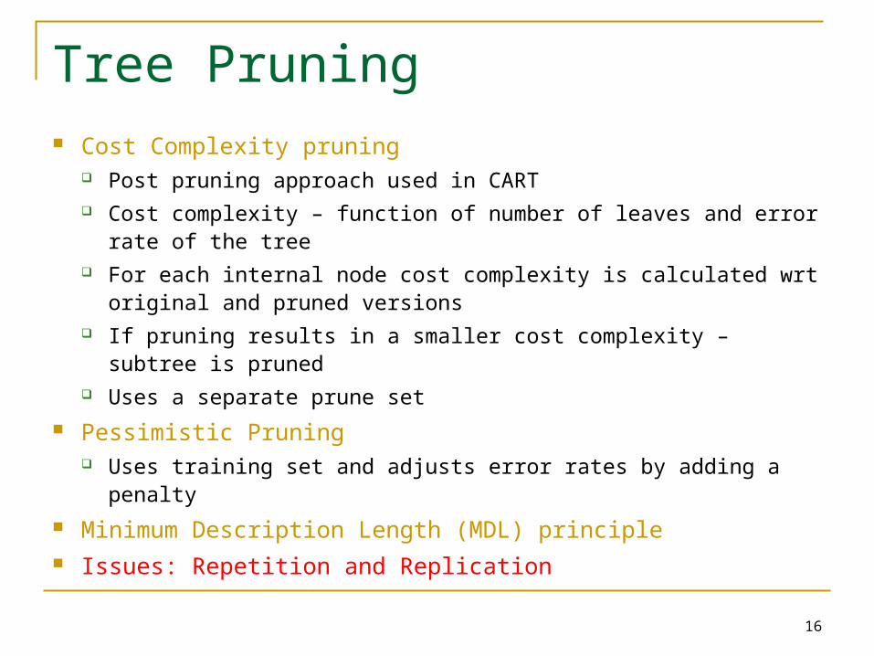
Tree Pruning Cost Complexity pruning
Post pruning approach used in CART Cost complexity – function of number of leaves and error rate of
the tree For each internal node cost complexity is calculated wrt original
and pruned versions If pruning results in a smaller cost complexity – subtree is pruned Uses a separate prune set
Pessimistic Pruning Uses training set and adjusts error rates by adding a penalty
Minimum Description Length (MDL) principle Issues: Repetition and Replication
17
Enhancements to Basic Decision Tree Induction
Allow for continuous-valued attributes Dynamically define new discrete-valued attributes that partition the
continuous attribute value into a discrete set of intervals Handle missing attribute values
Assign the most common value of the attribute Assign probability to each of the possible values
Attribute construction Create new attributes based on existing ones that are sparsely
represented This reduces fragmentation, repetition, and replication
18
Scalability and Decision Tree Induction
Scalability: Classifying data sets with millions of examples and hundreds of attributes with reasonable speed
Large scale databases – do not fit into memory Repeated Swapping of data – Inefficient Scalable Variants
SLIQ, SPRINT
19
Scalable Decision Tree Induction Methods
SLIQ Supervised Learning in Quest Presort the data Builds an index for each attribute and only class list and the current
attribute list reside in memory Each attribute has an associated attribute list indexed by a Record
Identifier (RID) – linked to class list Class list points to node Limited by the size of the class list
20
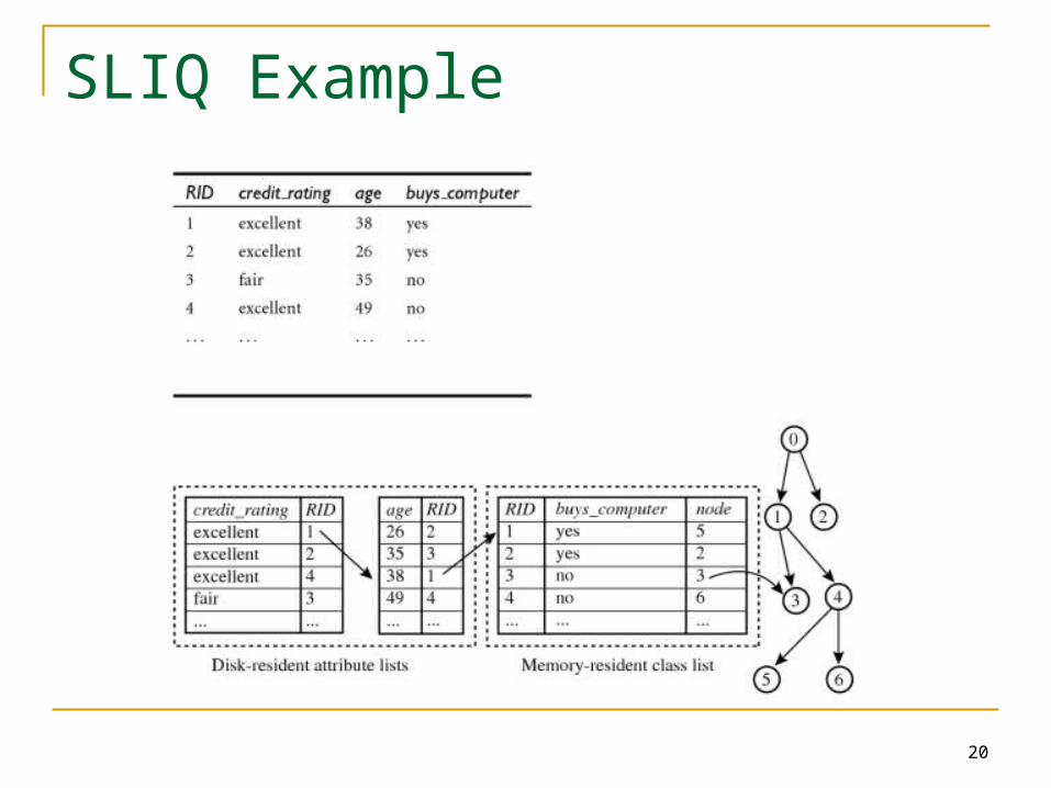
SLIQ Example
21
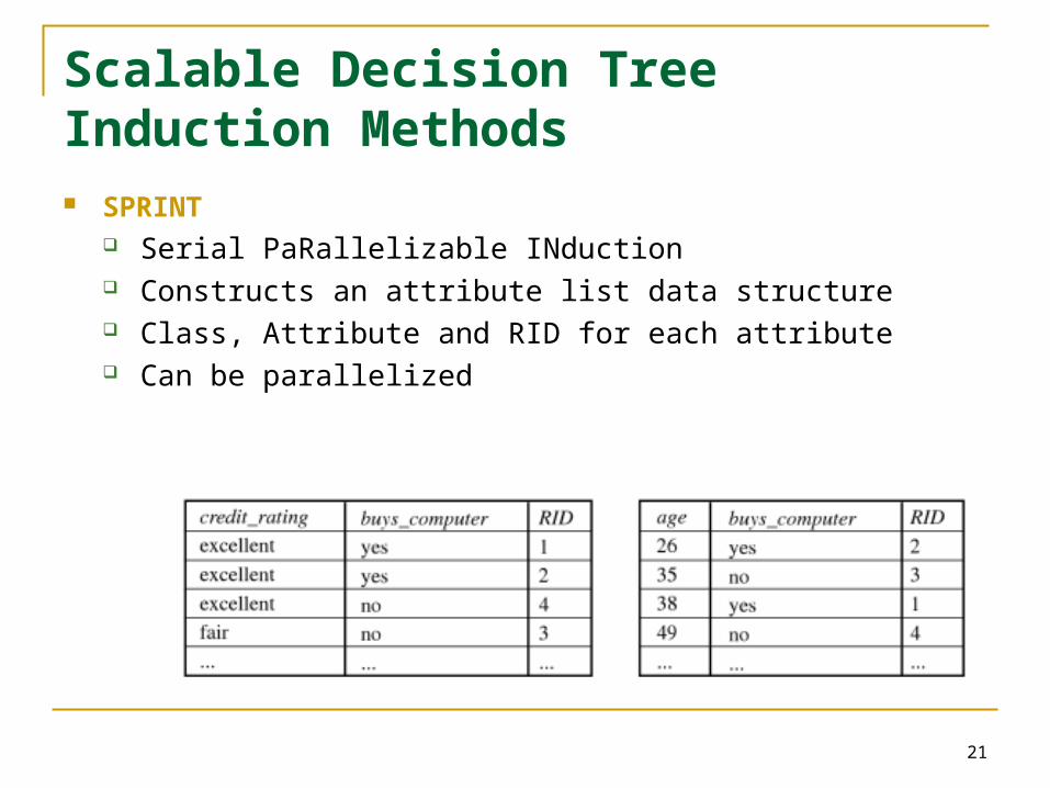
Scalable Decision Tree Induction Methods SPRINT
Serial PaRallelizable INduction Constructs an attribute list data structure Class, Attribute and RID for each attribute Can be parallelized
22
Scalability Framework for RainForest Separates the scalability aspects from the criteria that determine
the quality of the tree
Builds an AVC-list: AVC (Attribute, Value, Class_label)
AVC-set (of an attribute X )
Projection of training dataset onto the attribute X and class label
where counts of individual class label are aggregated
23
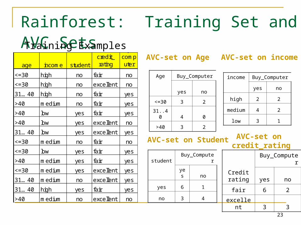
Rainforest: Training Set and AVC Sets
student Buy_Computer
yes no
yes 6 1
no 3 4
Age Buy_Computer
yes no
<=30 3 2
31..40 4 0
>40 3 2
Creditrating
Buy_Computer
yes no
fair 6 2
excellent 3 3
age income student
credit_ rating
buys_computer
<=30 high no fair no
<=30 high no excellent no
31…40 high no fair yes
>40 medium no fair yes
>40 low yes fair yes
>40 low yes excellent no
31…40 low yes excellent yes
<=30 medium no fair no
<=30 low yes fair yes
>40 medium yes fair yes
<=30 medium yes excellent yes
31…40 medium no excellent yes
31…40 high yes fair yes
>40 medium no excellent no
AVC-set on incomeAVC-set on Age
AVC-set on Student
Training Examples
income Buy_Computer
yes no
high 2 2
medium 4 2
low 3 1
AVC-set on credit_rating
24
BOAT (Bootstrapped Optimistic Algorithm for Tree Construction)
Use a statistical technique called bootstrapping to create several
smaller samples (subsets), each fits in memory
Each subset is used to create a tree, resulting in several trees
These trees are examined and used to construct a new tree T’
It turns out that T’ is very close to the tree that would be generated
using the whole data set together
Adv: requires only two scans of DB, an incremental algorithm
Very much faster