Embed Size (px)
Citation preview

Elizabeth SayedElizabeth StoltzfusDecember 4, 2002
Project 2 Presentation
Spatial DatabasesGIS Case Studies
UC Berkeley: IEOR 215

2
UC Berkeley: IEOR 215
Agenda
Spatial Database Basics
Geographic Information Systems (GIS) Basics
Case Studies

3
UC Berkeley: IEOR 215
Spatial Database Basics
Common applications

4
UC Berkeley: IEOR 215
Spatial Databases Background
Spatial databases provide structures for storage and analysis of spatial data
Spatial data is comprised of objects in multi-dimensional space
Storing spatial data in a standard database would require excessive amounts of space
Queries to retrieve and analyze spatial data from a standard database would be long and cumbersome leaving a lot of room for error
Spatial databases provide much more efficient storage, retrieval, and analysis of spatial data

5
UC Berkeley: IEOR 215
Types of Data Stored in Spatial Databases
Two-dimensional data examples
– Geographical
– Cartesian coordinates (2-D)
– Networks
– Direction
Three-dimensional data examples
– Weather
– Cartesian coordinates (3-D)
– Topological
– Satellite images

6
UC Berkeley: IEOR 215
Spatial Databases Uses and Users
Three types of uses
– Manage spatial data
– Analyze spatial data
– High level utilization
A few examples of users
– Transportation agency tracking projects
– Insurance risk manager considering location risk profiles
– Doctor comparing Magnetic Resonance Images (MRIs)
– Emergency response determining quickest route to victim
– Mobile phone companies tracking phone usage

7
UC Berkeley: IEOR 215
Spatial Databases Uses and Users
Three types of uses
– Manage spatial data
– Analyze spatial data
– High level utilization
A few examples of users
– Transportation agency tracking projects
– Insurance risk manager considering location risk profiles
– Doctor comparing Magnetic Resonance Images (MRIs)
– Emergency response determining quickest route to victim
– Mobile phone user determining current relative location of businesses

8
UC Berkeley: IEOR 215
Spatial Database Management System
Spatial Database Management System (SDBMS) provides the capabilities of a traditional database management system (DBMS) while allowing special storage and handling of spatial data.
SDBMS:
– Works with an underlying DBMS
– Allows spatial data models and types
– Supports querying language specific to spatial data types
– Provides handling of spatial data and operations

9
UC Berkeley: IEOR 215
SDBMS Three-layer Structure
SDBMS works with a spatial application at the front end and a DBMS at the back end
SDBMS has three layers:
– Interface to spatial application
– Core spatial functionality
– Interface to DBMS
Sp
ati
al
ap
pli
ca
tio
n
DB
MS
Inte
rfa
ce
to
DB
MS
Inte
rfa
ce
to
sp
ati
al
ap
pli
ca
tio
n
Core Spatial Functionality
Taxonomy
Data types
Operations
Query language
Algorithms
Access methods

10
UC Berkeley: IEOR 215
Spatial Query Language
Number of specialized adaptations of SQL
– Spatial query language
– Temporal query language (TSQL2)
– Object query language (OQL)
– Object oriented structured query language (O2SQL)
Spatial query language provides tools and structures specifically for working with spatial data
SQL3 provides 2D geospatial types and functions

11
UC Berkeley: IEOR 215
Spatial Query Language Operations
Three types of queries:
– Basic operations on all data types (e.g. IsEmpty, Envelope, Boundary)
– Topological/set operators (e.g. Disjoint, Touch, Contains)
– Spatial analysis (e.g. Distance, Intersection, SymmDiff)

12
UC Berkeley: IEOR 215
Spatial Data Entity Creation
Form an entity to hold county names, states, populations, and geographies
CREATE TABLE County(
Name varchar(30),
State varchar(30),
Pop Integer,
Shape Polygon);
Form an entity to hold river names, sources, lengths, and geographies
CREATE TABLE River(
Name varchar(30),
Source varchar(30),
Distance Integer,
Shape LineString);

13
UC Berkeley: IEOR 215
Example Spatial Query
Find all the counties that border on Contra Costa county
SELECT C1.Name
FROM County C1, County C2
WHERE Touch(C1.Shape, C2.Shape) = 1 AND C2.Name = ‘Contra Costa’;
Find all the counties through which the Merced river runs
SELECT C.Name, R.Name
FROM County C, River R
WHERE Intersect(C.Shape, R.Shape) = 1 AND R.Name = ‘Merced’;
CREATE TABLE County(
Name varchar(30),
State varchar(30),
Pop Integer,
Shape Polygon);
CREATE TABLE River(
Name varchar(30),
Source varchar(30),
Distance Integer,
Shape LineString);

14
UC Berkeley: IEOR 215
Geographic Information System (GIS) Basics
Common applications

15
UC Berkeley: IEOR 215
GIS Applications1. Cartographic
– Irrigation– Land evaluation– Crop Analysis– Air Quality– Traffic patterns– Planning and facilities management
2. Digital Terrain Modeling– Earth science resources– Civil Engineering & Military Evaluation– Soil Surveys– Pollution Studies– Flood Control
3. Geographic objects– Car navigation systems– Utility distribution and consumption– Consumer product and services

16
UC Berkeley: IEOR 215
GIS Data Format
Modeling
1. Vector – geometric objects such as points, lines and polygons
2. Raster – array of points
Analysis
1. Geomorphometric –slope values, gradients, aspects, convexity
2. Aggregation and expansion
3. Querying
Integration
1. Relationship and conversion among vector and raster data

17
UC Berkeley: IEOR 215
GIS – Data Modeling using Objects & Fields
Name Shape
Pine [(0,2), (4,2), (4,4), (0,4)]
Fir [(0,0), (2,0), (2,2), (0,2)]
Oak [(2,0), (4,0), (4,2), (2,2)
Pine
Fir Oak
(0,4)
(0,2)
(0,0) (2,0) (4,0)
Object Viewpoint Field Viewpoint
Pine: 0<x<4; 2<y<4
Fir: 0<x<2; 0<y<2
Oak: 2<x<4; 0<y<2
Source: “Spatial Pictogram Enhanced Data Models pg 79

18
UC Berkeley: IEOR 215
Conceptual Data Modeling
Relational Databases: ER diagram
Limitations for ER with respect to Spatial databases: – Can not capture semantics
– No notion of key attributes and unique OID’s in a field model
– ER Relationship between entities derived from application under consideration
– Spatial Relationships are inherent between objects
Solution: Pictograms for Spatial Conceptual Data-Modeling

19
UC Berkeley: IEOR 215
Pictograms - Shapes
Types: Basic Shapes, Multi-Shapes, Derived Shapes, Alternate Shapes, Any possible Shape, User-Defined Shapes
Basic Shapes Alternate Shapes
Multi-Shapes Any Possible Shape
Derived Shapes User Defined Shape
N 0, N
*
!
20
UC Berkeley: IEOR 215
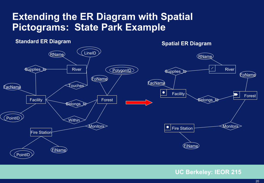
Extending the ER Diagram with Spatial Pictograms: State Park Example
ForestFacilityBelongs_to
River
Standard ER Diagram
Supplies_to
Fire Station
Monitors
LineID
PointID
PointID Within
Touches
FiName
FacName
RName
FoName
ForestFacility
Belongs_to
RiverSupplies_to
Fire Station Monitors
FiName
FacName
RName
FoName
Spatial ER Diagram
PolygonID

21
UC Berkeley: IEOR 215
Case Studies
Specific applications of spatial databases

22
UC Berkeley: IEOR 215
Case Study: Wetlands Objective: To predict the spatial distribution of the
location of bird nests in the wetlands
Location: Darr and Stubble on the shores of lake Erie in Ohio
Focus
1. Vegetation Durability
2. Distance to Open Water
3. Water Depth
Assumptions with Classical Data mining
1. Data is independently generated – no autocorrelation
2. Local vs. global trends
Spatial accuracy
1. Predictions vs. actual
2. Impact
P A
P P
A A
A
A
A
P
P P A
A A
Location of Nests
Actual Pixel Locations
Case 1:
Possible Prediction
Case 2:
Possible PredictionSource: What’s Spatial About Spatial Data Mining pg 490

23
UC Berkeley: IEOR 215
Case Study: Green House Gas Emission Estimations
Objective:
– To assess the impact of land-use and land cover changes on ground carbon stock and soil surface flux of CO2, N2O and CH4 in Jambi Province, Indonesia
Methodology:
– Initiated by development of land-use/land cover maps and followed by field measurements
– Spatial database construction development based on 1986 and 1992 land-use/land cover maps that developed from Landsat MSSR and SPOT
– Weight of sample components of the tree and streams, branches, twigs, etc were estimated from equations and literature
– Emission rates were developed by plotting and analyzing collected air samples
– Field data measurements and GIS spatial data were combined using a Look Up Table of Arc/Info.
Source: “Spatial Database Development for green house gas emission Estimation using remote sensing and GIS”
24
UC Berkeley: IEOR 215
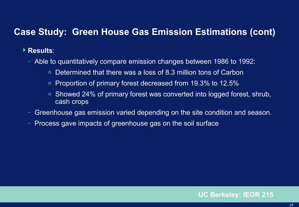
Case Study: Green House Gas Emission Estimations (cont)
Results:
– Able to quantitatively compare emission changes between 1986 to 1992:
o Determined that there was a loss of 8.3 million tons of Carbon
o Proportion of primary forest decreased from 19.3% to 12.5%
o Showed 24% of primary forest was converted into logged forest, shrub, cash crops
– Greenhouse gas emission varied depending on the site condition and season.
– Process gave impacts of greenhouse gas on the soil surface

25
UC Berkeley: IEOR 215
Case Study: Pantanal Area, Brazil
Objective: To assess the drastic land use changes in the Pantanal region since 1985
Data Source:
– 3 Landsat TM images of the Pantal study area from 1985, 1990, 1996
– A land-use survey from 1997
Assessment Methodology:
– Normalized Difference Vegetation Index (NDVI) was computed for each year
– NDVI maps of the three years combined and submitted to multi-dimensional image segmentation
– Classified vegetation
– Produced a color composite by year that identified the density of vegetation
Source: Integrated Spatial Databases pg 116

26
UC Berkeley: IEOR 215
Conclusion
Many varied applications of spatial databases
Stores spatial data in various formats specific to use
Captures spatial data more concisely
Enables more thorough understanding of data
Retrieves and manipulates spatial data more efficiently and effectively

27
UC Berkeley: IEOR 215

28
UC Berkeley: IEOR 215
Problem 1 Solution
a) Find all cities that are located within Marin County.
SELECT C2.Name
FROM County C1, City C2
WHERE Within(C1.Shape, C2.Shape) = 1 AND C1.Name = ‘Marin’;
b) Find any rivers that borders on Mendocino County.
SELECT R.Name
FROM County C, River R
WHERE Touch(C.Shape, R.Shape) = 1 AND C.Name = ‘Mendocino’;
c) Find the counties that do not touch on Orange County.
SELECT C1.Name
FROM County C1, County C2
WHERE Disjoint(C1.Shape, C2.Shape) = 1 AND C2.Name = ‘Orange’;

29
UC Berkeley: IEOR 215
Problem 2 Solution
Room
HallwayCloset
Furniture
Length
Name
RoomID
FurnID
HallID
Type
ClosetID
Belongs_To
Belongs_To
Belongs_To
Accesses