Toy interacting Model

Fabrizio Troilo (1067418), Hatice Kubra Bayram (1068770), Haleem ur Rahman (1067542)

June 30, 2016

1 The Model

The model represents an artificial toy economy, populated by n firms which produce a homogeneous

good. Firm individual output is based on a stochastic component which is normalized through the

average of firm shocks. Firm use all their net-worth in production.

Kit = NWit (1)

Thus, firm i net-worth (NWit) at time t is used as capital (Kit) for the production process. Potential

production depends on productivity (φ):

yit = φKit (2)

Revenues are given by an individual idiosyncratic shock (uit), normalized by the mean of the

idiosyncratic shocks that hit all the j firms.

(3)

The idiosyncratic shock is a random variable extracted from a uniform distribution:

uit ∼ U[umin,umax] (4)

Firm profit (πit) is given by revenues minus linear production costs (gKit) and a fixed component (F).

πit = yˆit − gKit – F (5)

Net-worth evolution depends on profits:

NWi,t+1 = NWi,t + πit (6)

If a firm has a non-positive net-worth, it exits from the economy and it is substituted by a new firm with

the initial net-worth value.

1.1 Model change: introducing dividends on profits

In a second moment, the original model has been modified introducing dividends on profits.

We assumed initially that 10% of profits are paid out to investors. As a result, the Net-worth of the

profitable companies will be reduced by 10% as compared to the original model, since not all the

profits will be reinvested in the production process.

As only profitable companies can yield dividends, we modified the model adding the following lines:

---------------------------------------

# firm profit

M$profit=M$effectiveSupply-g*M$netWorth-F

# introduce dividends on profits

ndiv=0;

for (i in 1:nfirm){

if (M$profit[i]>0){ #we look for the profitable firms only

ndiv=ndiv+1 #profitable firms counter for each cycle

M$profit[i]=M$profit[i]- δ*M$profit[i] #profits are reduced by δ% before being addedd to the NetWorh

}}

# equities update

M$netWorth=M$netWorth+M$profit #we reinvest only (1- δ)% of the profits

------------------------------------------

2. Original model analysis

We begin our analysis with the original model (with no dividends) in order to compare it with a toy

economy where profitable firms pay out dividends to investors.

The parameters values we used for the original model are the followings:

Table 1. Parameters (original model)

Parameters Values

nfirm 100

phi 1

F 0.1

g 0.99

netWorthInitial 10

ncycle 100

nrun 10

Umin 0.8

Umax 1.2

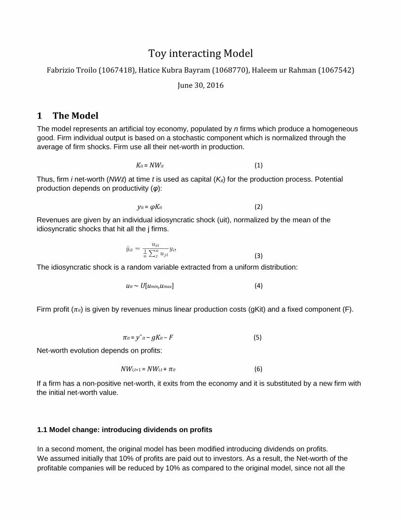
From run number 1 to run number 10, is possible to see two main patterns of the aggregate

production levels. Almost half of the runs present, initially, a decreasing trend in the level of aggregate

production (from cycle number 1 to about half of the cycles) and then a strongly increasing trend (from

the second part of the distribution onward). This kind of path is well represented by the graph of run

number 2. The other half of the runs instead, seem to have an ever-increasing trend, as represented

by the charter of run number 9.

Table 2 – Aggregate Production, Run 2 Table 3 – Aggregate Production, Run 9

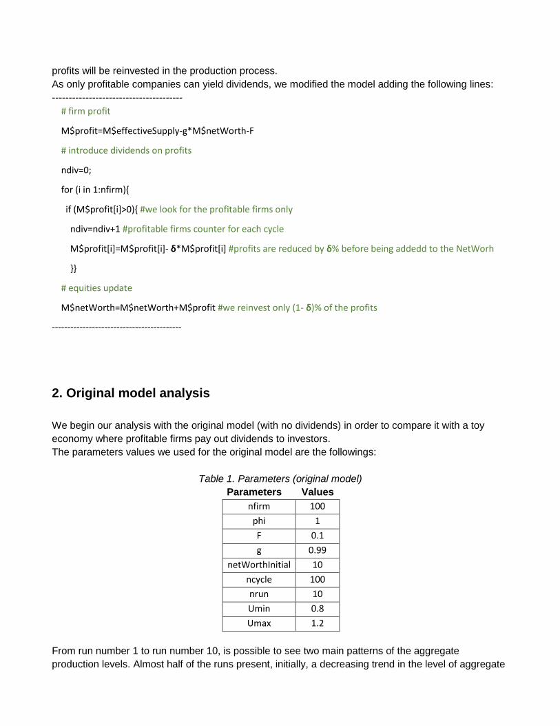
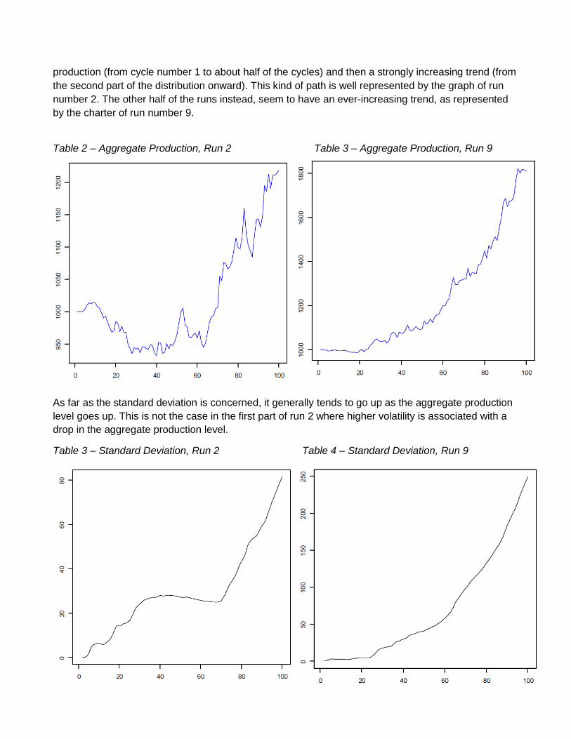
As far as the standard deviation is concerned, it generally tends to go up as the aggregate production

level goes up. This is not the case in the first part of run 2 where higher volatility is associated with a

drop in the aggregate production level.

Table 3 – Standard Deviation, Run 2 Table 4 – Standard Deviation, Run 9

0.00

50.00

100.00

150.00

200.00

250.00

300.00

350.00

400.00

0 2 4 6 8 10 12

Standard deviation

800

900

1000

1100

1200

1300

1400

0 2 4 6 8 10 12

Average Production

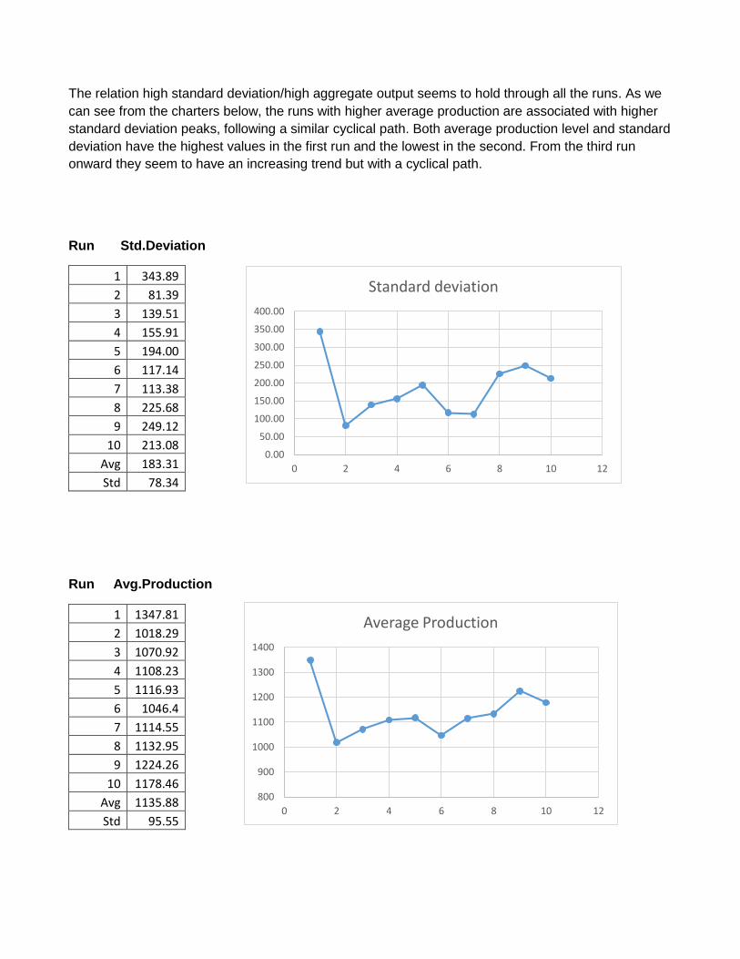
The relation high standard deviation/high aggregate output seems to hold through all the runs. As we

can see from the charters below, the runs with higher average production are associated with higher

standard deviation peaks, following a similar cyclical path. Both average production level and standard

deviation have the highest values in the first run and the lowest in the second. From the third run

onward they seem to have an increasing trend but with a cyclical path.

Run Std.Deviation

Run Avg.Production

1 343.89

2 81.39

3 139.51

4 155.91

5 194.00

6 117.14

7 113.38

8 225.68

9 249.12

10 213.08

Avg 183.31

Std 78.34

1 1347.81

2 1018.29

3 1070.92

4 1108.23

5 1116.93

6 1046.4

7 1114.55

8 1132.95

9 1224.26

10 1178.46

Avg 1135.88

Std 95.55

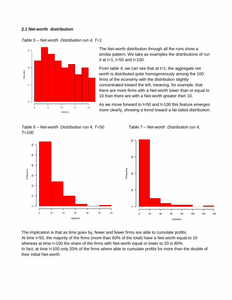
2.1 Net-worth distribution

Table 5 – Net-worth Distribution run 4, T=1

The Net-worth distribution through all the runs show a

similar pattern. We take as examples the distributions of run

4 at t=1, t=50 and t=100.

From table 4, we can see that at t=1, the aggregate net

worth is distributed quite homogeneously among the 100

firms of the economy with the distribution slightly

concentrated toward the left, meaning, for example, that

there are more firms with a Net-worth lower than or equal to

10 than there are with a Net-worth greater then 10.

As we move forward to t=50 and t=100 this feature emerges

more clearly, showing a trend toward a fat-tailed distribution.

Table 6 – Net-worth Distribution run 4, T=50 Table 7 – Net-worth Distribution run 4,

T=100

The implication is that as time goes by, fewer and fewer firms are able to cumulate profits.

At time t=50, the majority of the firms (more than 60% of the total) have a Net-worth equal to 10

whereas at time t=100 the share of the firms with Net-worth equal or lower to 20 is 80%.

In fact, at time t=100 only 20% of the firms where able to cumulate profits for more than the double of

their initial Net-worth.

3. Second step: introducing dividends on profits

The second step of our analysis aimed at identifying the evolution of the toy economy when

introducing dividends on profits. We start off by setting to 10% the share of the profits paid off to

shareholders for each cycle. Our intuition is that, since the Net-worth of the profitable companies will

accumulate at a rate 10% slower as compared to the original model, the economy might be more

sensitive to shocks and the aggregate production level of the economy will be lower at any given time.

Table 1. Parameters (original model)

Parameters Values

nfirm 100

phi 1

F 0.1

g 0.99

netWorthInitial 10

ncycle 100

nrun 10

Umin 0.8

Umax 1.2

δ 0.1

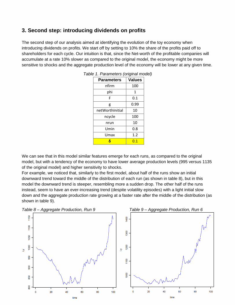
We can see that in this model similar features emerge for each runs, as compared to the original

model, but with a tendency of the economy to have lower average production levels (995 versus 1135

of the original model) and higher sensitivity to shocks.

For example, we noticed that, similarly to the first model, about half of the runs show an initial

downward trend toward the middle of the distribution of each run (as shown in table 8), but in this

model the downward trend is steeper, resembling more a sudden drop. The other half of the runs

instead, seem to have an ever-increasing trend (despite volatility episodes) with a light initial slow

down and the aggregate production rate growing at a faster rate after the middle of the distribution (as

shown in table 9).

Table 8 – Aggregate Production, Run 9 Table 9 – Aggregate Production, Run 6

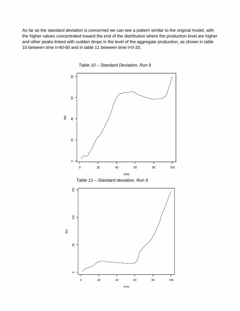
As far as the standard deviation is concerned we can see a pattern similar to the original model, with

the higher values concentrated toward the end of the distribution where the production level are higher

and other peaks linked with sudden drops in the level of the aggregate production, as shown in table

10 between time t=40-60 and in table 11 between time t=0-20.

Table 10 – Standard Deviation, Run 9

Table 11 – Standard deviation, Run 6

800.00

850.00

900.00

950.00

1000.00

1050.00

1100.00

1150.00

1200.00

0 2 4 6 8 10 12

Average Production

0

50

100

150

200

250

0 2 4 6 8 10 12

Deviazione Standard

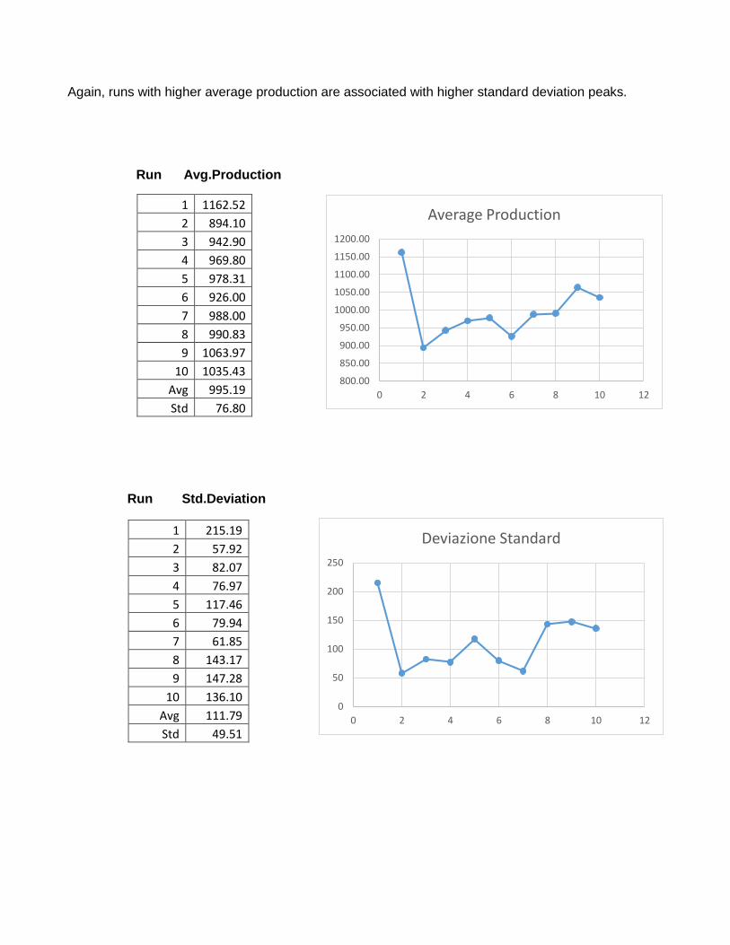
Again, runs with higher average production are associated with higher standard deviation peaks.

Run Avg.Production

Run Std.Deviation

1 1162.52

2 894.10

3 942.90

4 969.80

5 978.31

6 926.00

7 988.00

8 990.83

9 1063.97

10 1035.43

Avg 995.19

Std 76.80

1 215.19

2 57.92

3 82.07

4 76.97

5 117.46

6 79.94

7 61.85

8 143.17

9 147.28

10 136.10

Avg 111.79

Std 49.51

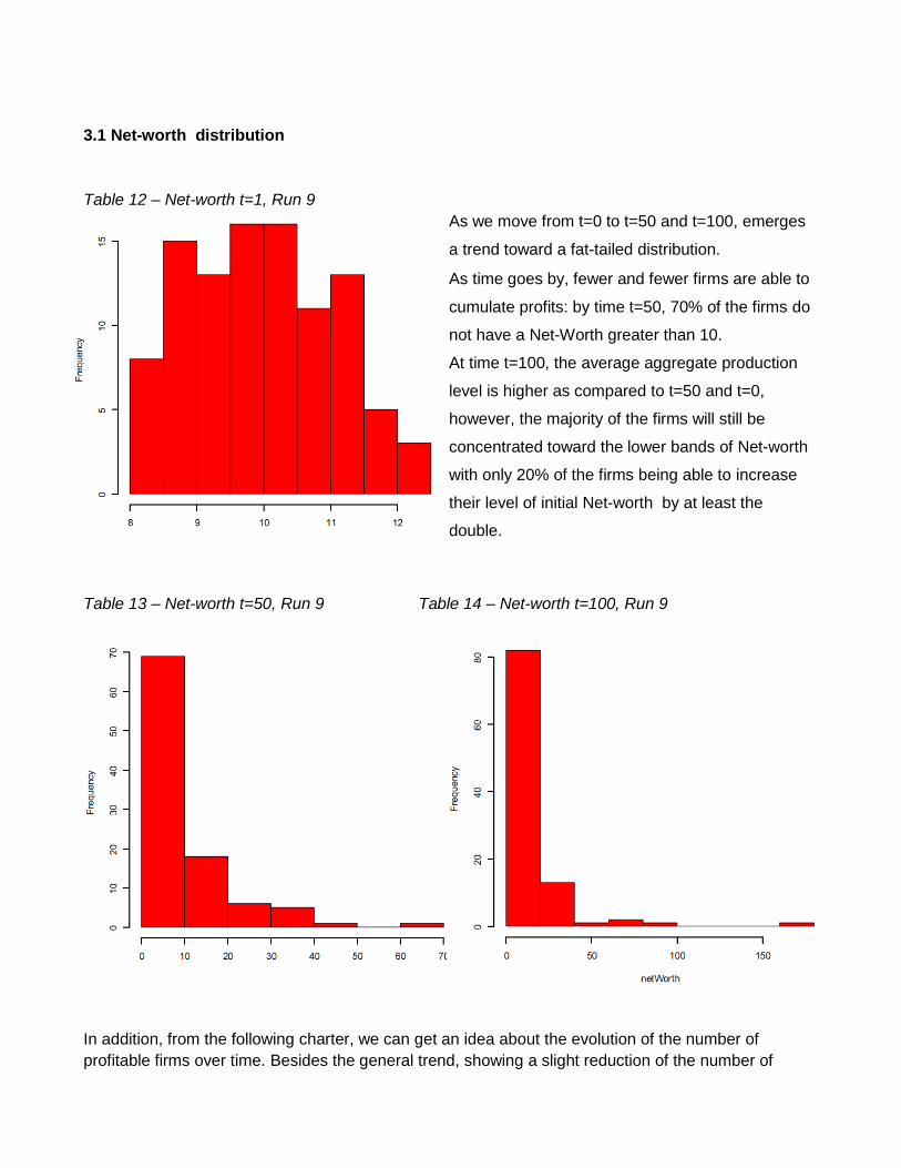
3.1 Net-worth distribution

Table 12 – Net-worth t=1, Run 9

As we move from t=0 to t=50 and t=100, emerges

a trend toward a fat-tailed distribution.

As time goes by, fewer and fewer firms are able to

cumulate profits: by time t=50, 70% of the firms do

not have a Net-Worth greater than 10.

At time t=100, the average aggregate production

level is higher as compared to t=50 and t=0,

however, the majority of the firms will still be

concentrated toward the lower bands of Net-worth

with only 20% of the firms being able to increase

their level of initial Net-worth by at least the

double.

Table 13 – Net-worth t=50, Run 9 Table 14 – Net-worth t=100, Run 9

In addition, from the following charter, we can get an idea about the evolution of the number of

profitable firms over time. Besides the general trend, showing a slight reduction of the number of

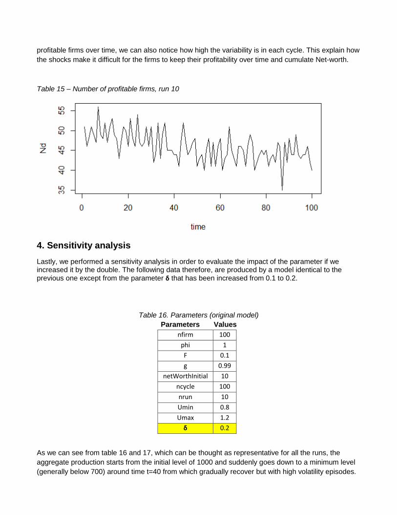
profitable firms over time, we can also notice how high the variability is in each cycle. This explain how

the shocks make it difficult for the firms to keep their profitability over time and cumulate Net-worth.

Table 15 – Number of profitable firms, run 10

4. Sensitivity analysis

Lastly, we performed a sensitivity analysis in order to evaluate the impact of the parameter if we increased it by the double. The following data therefore, are produced by a model identical to the previous one except from the parameter δ that has been increased from 0.1 to 0.2.

Table 16. Parameters (original model)

Parameters Values

nfirm 100

phi 1

F 0.1

g 0.99

netWorthInitial 10

ncycle 100

nrun 10

Umin 0.8

Umax 1.2

δ 0.2

As we can see from table 16 and 17, which can be thought as representative for all the runs, the

aggregate production starts from the initial level of 1000 and suddenly goes down to a minimum level

(generally below 700) around time t=40 from which gradually recover but with high volatility episodes.

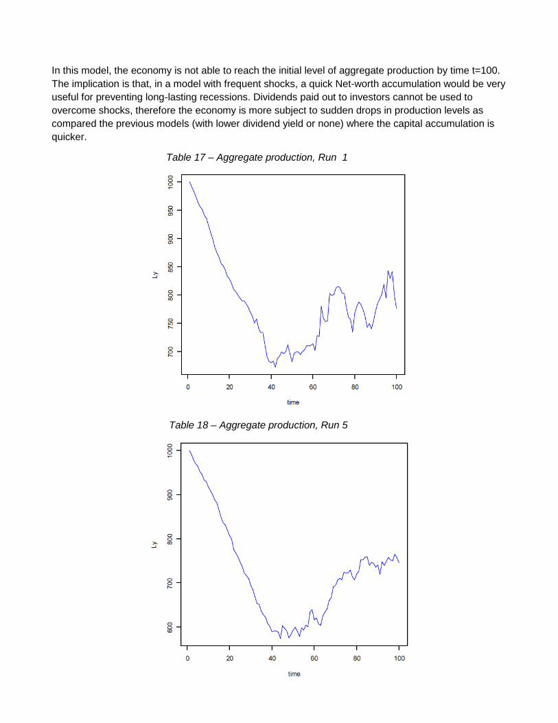
In this model, the economy is not able to reach the initial level of aggregate production by time t=100.

The implication is that, in a model with frequent shocks, a quick Net-worth accumulation would be very

useful for preventing long-lasting recessions. Dividends paid out to investors cannot be used to

overcome shocks, therefore the economy is more subject to sudden drops in production levels as

compared the previous models (with lower dividend yield or none) where the capital accumulation is

quicker.

Table 17 – Aggregate production, Run 1

Table 18 – Aggregate production, Run 5

680.00

700.00

720.00

740.00

760.00

780.00

800.00

0 2 4 6 8 10 12

Average Production

70.00

80.00

90.00

100.00

110.00

120.00

130.00

140.00

0 2 4 6 8 10 12

Deviazione Standard

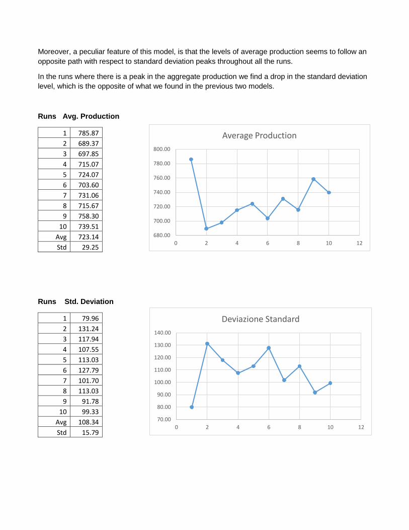
Moreover, a peculiar feature of this model, is that the levels of average production seems to follow an

opposite path with respect to standard deviation peaks throughout all the runs.

In the runs where there is a peak in the aggregate production we find a drop in the standard deviation

level, which is the opposite of what we found in the previous two models.

Runs Avg. Production

Runs Std. Deviation

1 79.96

2 131.24

3 117.94

4 107.55

5 113.03

6 127.79

7 101.70

8 113.03

9 91.78

10 99.33

Avg 108.34

Std 15.79

1 785.87

2 689.37

3 697.85

4 715.07

5 724.07

6 703.60

7 731.06

8 715.67

9 758.30

10 739.51

Avg 723.14

Std 29.25

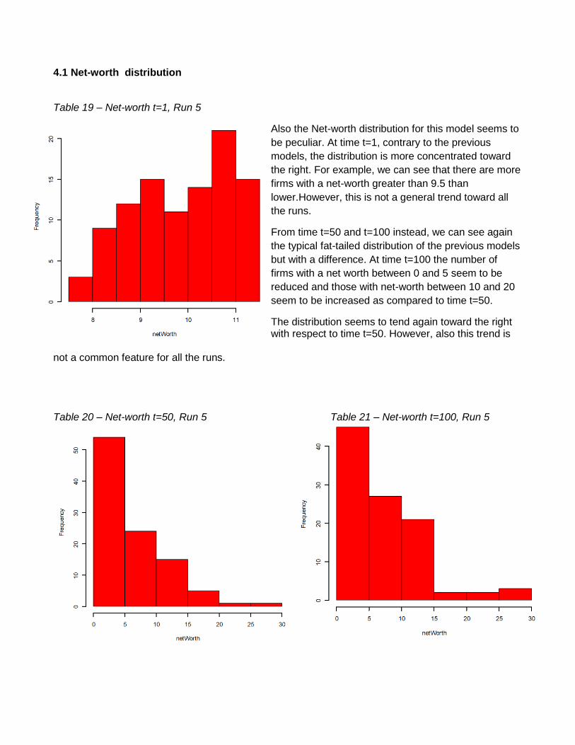
4.1 Net-worth distribution

Table 19 – Net-worth t=1, Run 5

Also the Net-worth distribution for this model seems to

be peculiar. At time t=1, contrary to the previous

models, the distribution is more concentrated toward

the right. For example, we can see that there are more

firms with a net-worth greater than 9.5 than

lower.However, this is not a general trend toward all

the runs.

From time t=50 and t=100 instead, we can see again

the typical fat-tailed distribution of the previous models

but with a difference. At time t=100 the number of

firms with a net worth between 0 and 5 seem to be

reduced and those with net-worth between 10 and 20

seem to be increased as compared to time t=50.

The distribution seems to tend again toward the right with respect to time t=50. However, also this trend is

not a common feature for all the runs. Table 20 – Net-worth t=50, Run 5 Table 21 – Net-worth t=100, Run 5

5. Concluding remarks

In this paper we presented an artificial toy economy in order to investigate the impact of idiosyncratic shocks on the production and the net-worth of firms. We then introduced dividends on profits to see what evolutions could emerge. Since the net-worths for of each period are given by the net-worth of the previous period plus profits, dividends reduce the ability of profitable firms to cumulate net-worth over time hence producing less over the same period with respect to the firms of the original model. We have seen that, with a dividend level of 0.1, the economy decrease on average its aggregate production level and it is more sensitive to shocks. This feature emerges even more clearly from the sensitivity analysis. Increasing dividends from 0.1 to 0.2, the economy experience a sudden drop and is not even able to go back to the initial level of aggregate production by time t=100. Dividends paid out to investors cannot be used to overcome shocks, therefore the economy is more subject to sudden drops in production levels as compared the previous models (with lower dividend yield or none) where the capital accumulation is quicker.