Spillover Dynamics Spillover Dynamics Spillover Dynamics Spillover Dynamics forforforfor

SystemicSystemicSystemicSystemic RiskRiskRiskRisk Measurement Measurement Measurement Measurement

Using Spatial Financial Time Using Spatial Financial Time Using Spatial Financial Time Using Spatial Financial Time

Series ModelsSeries ModelsSeries ModelsSeries Models

SYstemic Risk TOmography:

Signals, Measurements, Transmission Channels, and Policy Interventions

Francisco Blasques (a,b)

Siem Jan Koopman (a,b,c)

Andre Lucas (a,b,d)

Julia Schaumburg (a,b)

(a)VU University Amsterdam (b)Tinbergen Institute (c)CREATES (d)Duisenberg School of Finance

EFMA NyenrodeJune 2015

Introduction 3

This project: four main research questions

I What is the effectiveness of non-standard monetary policy onmarkets’ perceptions of sovereign credit risk interconnectedness?

I Can international debt interconnections be identified empirically aspossible transmission channels for systemic risk using economicdistances in a spatial analysis?

I Is the economic significance of these channels stable or does it varyover time and with economic conditions?

I What are the empirical cross-sectional interactions as well ascountry-specific and Europe-wide credit risk factors for Europeansovereigns?

Spatial GAS

Introduction 4

Systemic risk: multi-faceted

I Direct interconnectedness via cross-exposures

I Common asset exposures and fire-sales commonalities

I Global imbalances

I Liability vulnerability (stable funding ratios, CoCos, etc.)

I Sovereign and financial sector feedback loops

I Shadow banking feedback

I Real effects . . . ?

Spatial GAS

Introduction 5

Systemic sovereign credit risk

Systemic risk: Breakdown risk ofthe financial system induced by theinterdependence of its constituents.

European sovereign debt since 2009:

I Strong increases and comovements of credit spreads.I Financial interconnectedness across borders due to mutual

borrowing and lending

+ bailout engagements.

⇒ Spillovers of shocks between member states.

⇒ Unstable environment: need for time-varying parameter models andfat tails.

Spatial GAS

Introduction 6

Four European sovereign CDS spreads

Spatial GAS

Introduction 7

Other ‘goodies’ in this paper

I New parsimonious econometric model for overall time-varyingstrength of cross-sectional spillovers in credit spreads (systemic risk).⇒ Useful for flexible monitoring of policy measure effects.

I Dynamic spatial dependence model with time-varying parameters,accounting for typical data properties in finance (fat-tails,time-varying volatility): score driven models

I Econometric theory: asymptotic and finite sample properties of theML estimator of this ’spatial score driven model’

Spatial GAS

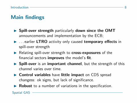
Introduction 8

Main findings

I Spill-over strength particularly down since the OMTannouncements and implementation by the ECB;

I . . . earlier LTRO activity only caused temporary effects inspill-over strength

I Relating spill-over strength to cross-exposures of thefinancial sectors improves the model’s fit.

I Spill-over is an important channel, but the strength of thischannel varies over time.

I Control variables have little impact on CDS spreadchangess: ok signs, but lack of significance.

I Robust to a number of variations in the specification.

Spatial GAS

Introduction 9

Related literature (partial and incomplete)

I Systemic risk in sovereign credit markets:

. Ang/Longstaff (2013), Lucas/Schwaab/Zhang (2013),

Aretzki/Candelon/Sy (2011), Kalbaska/Gatkowski (2012), De Santis

(2012), Caporin et al. (2014), Korte/Steffen (2013),

Kallestrup/Lando/Murgoci (2013), Beetsma et al. (2013, 2014).

I Spatial econometrics:

. General: Cliff/Ord (1973), Anselin (1988), Cressie (1993), LeSage/Pace(2009), Ord (1975), Lee (2004), Elhorst (2003);

. Panel data: Kelejian/Prucha (2010), Yu/de Jong/Lee (2008, 2012),Baltagi et al. (2007, 2013), Kapoor/Kelejian/Prucha (2007);

. Empirical finance: Keiler/Eder (2013), Fernandez (2011),

Asgarian/Hess/Liu (2013), Arnold/Stahlberg/Wied (2013), Wied (2012),

Denbee/Julliard/Li/Yuan (2013), Saldias (2013).

Spatial GAS

Spatial lag model 10

Modeling framework

Spatial GAS

Spatial lag model 11

Basic spatial lag model

Let y denote a vector of observations of a dependent variable for n units.A basic spatial lag model of order one is given by

y = ρWy︸︷︷︸’spatial lag’

+Xβ + e, e ∼ N(0, σ2In), (1)

where

I W is a nonstochastic (n × n) matrix of spatial weights with rows addingup to one and with zeros on the main diagonal,

I X is a (n × k)-matrix of covariates,

I |ρ| < 1, σ2 > 0, and β = (β1, ..., βk)′ are unknown coefficients.

Model (1) for observation i :

yi = ρn∑

j=1

wijyj +K∑

k=1

xikβk + ei (2)

Spatial GAS

Spatial lag model 12

Spatial spillovers (LeSage/Pace (2009))

Rewriting model (1) as

y = (In − ρW )−1Xβ + (In − ρW )−1e (3)

and expanding the inverse matrix as a power series yields

y = Xβ + ρWXβ + ρ2W 2Xβ + · · ·+ e + ρWe + ρ2W 2e + · · ·

Implications:

I The model is nonlinear in ρ.

I Each unit with a neighbor is its own second-order neighbor.

I The model can be interpreted as a structural VAR model with restrictedparameters.

Spatial GAS

Spatial lag model 13

Spatial models in empirical finance

I Spatial lag models: Keiler/Eder (2013), Fernandez (2011),Asgarian/Hess/Liu (2013), Arnold/Stahlberg/Wied (2013),Wied (2012).

I Spatial error models: Denbee/Julliard/Li/Yuan (2013),Saldias (2013).

I CDS application: Unrealistic to assume that systemicsovereign credit risk is static over time.

I So far, no model for time-varying spatial dependenceparameter in the literature.

Spatial GAS

Spatial GAS 14

Dynamic spatial dependence

I Idea: Let the strength of spillovers ρ change over time.

I GAS-SAR model for panel data, i = 1, ..., n, and t = 1, ...,T :

yt = ρtWyt + Xtβ + et , et ∼ pe(0,Σ), or

yt = ZtXtβ + Ztet ,

where Zt = (In − ρtW )−1, and pe corresponds to the error distribution,e.g. pe = N or pe = tν , with covariance matrix Σ.

I The model can be estimated by maximizing

` =T∑t=1

`t =T∑t=1

(ln pe(yt − ρtWyt − Xtβ;λ) + ln |(In − ρtW )|) , (4)

where λ is a vector of variance parameters.

I Ensure that ln |(In − ρtW )| exists: ρt = h(ft) = γ tanh(ft), γ < 1.

Spatial GAS

Spatial GAS 15

GAS dynamics for ρt

I Reparamerization: ρt = h(ft) = tanh(ft).

I ft is assumed to follow a dynamic process,

ft+1 = ω + ast + bft ,

where ω, a, b are unknown parameters.

I We specify st as the first derivative (“score”) of the predictive likelihoodw.r.t. ft (Creal/Koopman/Lucas, 2013).

I Model can be estimated straightforwardly by maximum likelihood (ML).

I For theory and empirics on different GAS/DCS models, see also, e.g.,Creal/Koopman/Lucas (2011), Harvey (2013), Harvey/Luati (2014),Blasques/Koopman/Lucas (2012, 2014a, 2014b).

Spatial GAS

Spatial GAS 16

Score

Score for Spatial GAS model with normal errors:

εt = yt − ρtWyt − Xtβ

st =(wt · y ′tW ′Σ−1εt − tr(ZtW )

)· h′(ft)

wt = 1

Spatial GAS

Spatial GAS 17

Score

Score for Spatial GAS model with t-errors:

εt = yt − ρtWyt − Xtβ

st =(wt · y ′tW ′Σ−1εt − tr(ZtW )

)· h′(ft)

wt =1 + n

ν

1+ 1νε′tΣ−1εt

Spatial GAS

Theory 18

Theory for Spatial GAS model

I Extension of theoretical results on GAS models inBlasques/Koopman/Lucas (2014a, 2014b):

I Nonstandard due to nonlinearity of the model, particularly in thecase of Spatial GAS-t specification.

I Conditions:

. moment conditions;

. b + a ∂st∂ftis contracting on average.

I Result: strong consistency and asymptotic normality of MLestimator.

I Also: Optimality results (see paper).

Spatial GAS

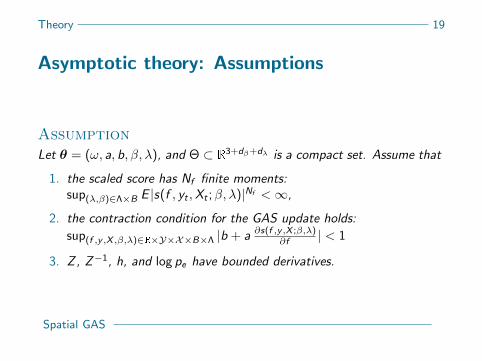
Theory 19

Asymptotic theory: Assumptions

AssumptionLet θ = (ω, a, b, β, λ), and Θ ⊂ R

3+dβ+dλ is a compact set. Assume that

1. the scaled score has Nf finite moments:sup(λ,β)∈Λ×B E |s(f , yt ,Xt ;β, λ)|Nf <∞,

2. the contraction condition for the GAS update holds:

sup(f ,y ,X ,β,λ)∈R×Y×X×B×Λ |b + a ∂s(f ,y ,X ;β,λ)∂f | < 1

3. Z , Z−1, h, and log pe have bounded derivatives.

Spatial GAS

Theory 20

Asymptotic theory: Results

Theorem(Consistency)Let {yt}t∈Z and {Xt}t∈Z be stationary and ergodic sequences satisfyingE |yt |Ny <∞ and E |Xt |Nx <∞ for some Ny > 0 and Nx > 0. Furthermore, letθ0 ∈ int(Θ) be the unique maximizer of `∞(θ) on Θ. Assume additionally that

Assumption holds. Then the MLE satisfies θ̂T (f1)a.s.→ θ0 as T →∞ for every

initialization value f1.

(Asymptotic Normality)Under the above assumptions and some additional moment conditions,

√T (θ̂T (f1)− θ0)

d→ N(0, I−1(θ0)J (θ0)I−1(θ0)

)as T →∞,

where J (θ0) := E˜̀′t(θ0)˜̀′t(θ0)> is the mean outer product of gradients and

I(θ0) := E˜̀′′t (θ0) is the Fisher information matrix.

Spatial GAS

Simulation 21

Simulation results (n = 9, T = 500)

0 100 200 300 400 500

0.0

0.4

0.8

Sine, dense W, t−errorsrh

o.t

0 100 200 300 400 500

0.0

0.2

0.4

0.6

0.8

1.0

Step, dense W, t−errors

rho.

t

Spatial GAS

Simulation 22

Simulation results I

0 100 200 300 400 500

0.86

0.90

0.94

Constant, dense W, t−errors

rho.

t

0 100 200 300 400 500

0.0

0.2

0.4

0.6

0.8

1.0

Sine, dense W, t−errors

rho.

t

0 100 200 300 400 500

0.0

0.2

0.4

0.6

0.8

1.0

Fast sine, dense W, t−errors

rho.

t

0 100 200 300 400 500

0.0

0.2

0.4

0.6

0.8

1.0

Step, dense W, t−errors

rho.

t

0 100 200 300 400 500

0.0

0.2

0.4

0.6

0.8

1.0

Ramp, dense W, t−errors

rho.

t

Spatial GAS

Simulation 23

Simulation: Consistency check

I Simulate from GAS model, check whether parameters areestimated consistently.

I DGP:

yt = ZtXtβ + Ztet , et ∼ i .i .d .N(0, σ2In).

I Parameters: ω = 0.05, a = 0.05, b = 0.8, β = 1.5, andσ2 = 2.

I Sample sizes: N = 9, T = { 500, 1000, 2000} .

I 500 replications.

Spatial GAS

Simulation 24

Simulation results II

0.02 0.04 0.06 0.08 0.10

010

2030

4050

6070

Density of estimates for ω, true value=0.05

N = 500 Bandwidth = 0.002946

Den

sity

T=500T=1000T=2000

0.040 0.045 0.050 0.055 0.060

050

150

250

350

Density of estimates for a, true value=0.0.05

N = 500 Bandwidth = 0.0006868

Den

sity

T=500T=1000T=2000

0.70 0.75 0.80 0.85 0.90

010

2030

40

Density of estimates for b, true value=0.8

N = 500 Bandwidth = 0.00627

Den

sity

T=500T=1000T=2000

1.46 1.48 1.50 1.52 1.54

010

2030

4050

60

Density of estimates for β, true value=1.5

N = 500 Bandwidth = 0.003423

Den

sity

T=500T=1000T=2000

1.85 1.90 1.95 2.00 2.05 2.10 2.15

05

1015

20

Density of estimates for σ2, true value=2

N = 500 Bandwidth = 0.01108

Den

sity

T=500T=1000T=2000

Spatial GAS

Application 25

Systemic risk in European credit spreads:Data

I Daily log changes in CDS spreads from February 2, 2009 - May 12,2014 (1375 observations).

I 8 European countries: Belgium, France, Germany, Ireland, Italy,Netherlands, Portugal, Spain.

I Country-specific covariates (lags):

. returns from leading stock indices,

. changes of 10-year government bond yields.

I Europe-wide control variables (lags):

. term spread: difference between three-month Euribor and EONIA,

. interbank interest rate: change in three-month Euribor,

. change in volatility index VSTOXX.

Spatial GAS

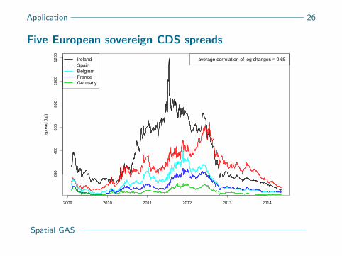
Application 26

Five European sovereign CDS spreads

2009 2010 2011 2012 2013 2014

200

400

600

800

1000

1200

spre

ad (

bp)

IrelandSpainBelgiumFranceGermany

average correlation of log changes = 0.65

Spatial GAS

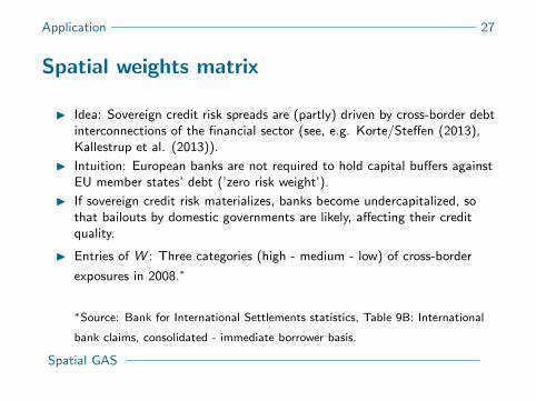
Application 27

Spatial weights matrix

I Idea: Sovereign credit risk spreads are (partly) driven by cross-border debtinterconnections of the financial sector (see, e.g. Korte/Steffen (2013),Kallestrup et al. (2013)).

I Intuition: European banks are not required to hold capital buffers againstEU member states’ debt (’zero risk weight’).

I If sovereign credit risk materializes, banks become undercapitalized, sothat bailouts by domestic governments are likely, affecting their creditquality.

I Entries of W : Three categories (high - medium - low) of cross-border

exposures in 2008.∗

∗Source: Bank for International Settlements statistics, Table 9B: International

bank claims, consolidated - immediate borrower basis.

Spatial GAS

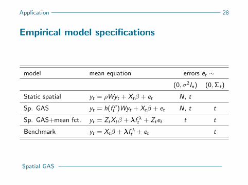
Application 28

Empirical model specifications

model mean equation errors et ∼

(0, σ2In) (0,Σt)

Static spatial yt = ρWyt + Xtβ + et N, t

Sp. GAS yt = h(f ρt )Wyt + Xtβ + et N, t t

Sp. GAS+mean fct. yt = ZtXtβ + λf λt + Ztet t t

Benchmark yt = Xtβ + λf λt + et t

Spatial GAS

Application 29

Model fit comparison

Static spatial Time-varying spatial

et ∼ N(0, σ2In) tλ(0, σ2In) N(0, σ2In) tλ(0, σ2In)

logL -26396.63 -24574.48 -26244.45 -24506.11

AICc 52807.35 49165.06 52507.03 49032.39

Time-varying spatial-t Benchmark-t

(+tv. volas) (+tv.volas) (+tv.volas)

(+mean f.) (+mean f.)

logL -24175.70 -24156.96 -26936.15

AICc 48389.97 48375.30 53927.42

Spatial GAS

Application 30

Parameter estimates

I Spatial dependence is high and significant.

I Spatial GAS parameters:

. High persistence of dynamic factors reflected by largeestimates for b.

. Estimates for score impact parameters a are small butsignificant.

I Estimates for β have expected signs.

I Mean factor loadings:

. Positive for Ireland, Portugal, Spain.

. Negative for Belgium, Italy, France, Germany, Netherlands.

Spatial GAS

Application 31

Estimation results: Full model

ωλ -0.0012 ωσ1 Belgium 0.0426 ω 0.0307

Aλ 0.3494 ωσ2 France 0.0448 A 0.0190

Bλ 0.6891 ωσ3 Germany 0.0573 B 0.9636

λ1 Belgium -0.2776 ωσ4 Ireland 0.0301 const. -0.0621

λ2 France -0.2846 ωσ5 Italy 0.0471 VStoxx -0.0257

λ3 Germany -0.2029 ωσ6 Netherlands 0.0443 term sp. 0.0693

λ4 Ireland 0.4050 ωσ7 Portugal 0.0524 stocks -0.1020

λ5 Italy -0.1604 ωσ8 Spain 0.0591 yields 0.0173

λ6 Netherlands -0.1891 Aσ 0.1826 λ0 3.1357

λ7 Portugal 0.4614 Bσ 0.9479

λ8 Spain 0.0988 logLik -24156.96AICc 48375.30

Spatial GAS

Application 32

Residual diagnostics: Full model

Test for remaining autocorrelation and ARCH effects in standardized residualsfrom full model (Spatial GAS+volas+mean factor)

sovereign LB test stat. ARCH LM test stat. average cross-corr.raw residuals raw residuals raw residuals

Belgium 108.64 15.93 169.91 25.53 0.70 0.07France 49.48 30.42 160.44 43.32 0.66 -0.01Germany 62.61 19.49 142.70 53.78 0.63 -0.07Ireland 129.89 17.53 302.23 87.11 0.64 -0.07Italy 99.02 42.43 102.13 150.88 0.71 0.08Netherlands 55.69 33.29 124.41 20.96 0.64 -0.05Portugal 167.91 32.56 189.35 56.89 0.65 0.03Spain 105.81 48.88 253.68 154.42 0.69 0.06

Spatial GAS

Application 33

Different choices of W

Candidates (all row-normalized):

I Raw exposure data (constant): Wraw

I Raw exposure data (updated quarterly): Wdyn

I Three categories of exposure amounts (high, medium, low): Wcat

I Exposures standardized by GDP: Wgdp

I Geographical neighborhood (binary, symmetric): Wgeo

Model fit comparison (only t-GAS model):

Wraw Wdyn Wcat Wgeo

logL -24745.56 -24679.44 -24506.11 -25556.85

Parameter estimates are robust.

Spatial GAS

Application 33

Different choices of W

Candidates (all row-normalized):

I Raw exposure data (constant): Wraw

I Raw exposure data (updated quarterly): Wdyn

I Three categories of exposure amounts (high, medium, low): Wcat

I Exposures standardized by GDP: Wgdp

I Geographical neighborhood (binary, symmetric): Wgeo

Model fit comparison (only t-GAS model):

Wraw Wdyn Wcat Wgeo

logL -24745.56 -24679.44 -24506.11 -25556.85

Parameter estimates are robust.

Spatial GAS

Application 34

Spillover strength 2009-2014

Spatial GAS

Conclusions 35

Conclusions

I Decrease of systemic risk from mid-2012 onwards; possiblydue to believable EU governments’ and ECB’s measures

I European sovereign CDS spreads are strongly spatiallydependent via cross-exposure channel, but the channel’sstrength may vary over time

I Spatial model with dynamic spillover strength and fat tails isnew, and it works (theory, simulation, empirics).

I Best model: Time-varying spatial dependence based ont-distributed errors, time-varying volatilities, additional meanfactor, and categorical spatial weights.

Spatial GAS

This project has received funding from the European Union’s

Seventh Framework Programme for research, technological

development and demonstration under grant agreement no° 320270

www.syrtoproject.eu

This document reflects only the author’s views.

The European Union is not liable for any use that may be made of the information contained therein.